DETERMINANTS OF POPULATION AND JOBS AT A LOCAL LEVEL:

AN APPLICATION FOR CATALAN MUNICIPALITIES*

Josep Mª Arauzo**

WP-EC 2002-25

Correspondence to: Josep Maria Arauzo Carod, Departament d'Economia, Facultat de Ciències Econòmiques i Empresarials, Universitat Rovira i Virgili, Av. de la Universitat, 1, 43204 – REUS, Tel. +34 977 759 800, Fax +34 977 759 810, correu-e: jmac@fcee.urv.es

Editor: Instituto Valenciano de Investigaciones Económicas, S.A.

Primera Edición Septiembre 2002

Depósito Legal: V-3616-2002

IVIE working papers offer in advance the results of economic research under way in order to encourage a discussion process before sending them to scientific journals for their final publication.

* This research was partially funded by the CICYT (SEC2000–0882–C02–02). I would like to acknowledge the helpful and supportive comments of Agustí Segarra and Miguel Manjón and the suggestions of one anonymous referee. I am also grateful to the Centre for Spatial and Real State Economics (CSpREE) of the University of Reading, where this paper was finished during my stay as a research visitor. Any errors are, of course, my own.

** Departament d’Economia, Universitat Rovira i Virgili.

2

DETERMINANTS OF POPULATION AND JOBS AT A LOCAL LEVEL: AN APPLICATION FOR CATALAN MUNICIPALITIES

Josep Mª Arauzo

ABSTRACT

This paper explores the determinants of population and jobs. We consider that employment and population are simultaneously determined and assume that for population and employees, location determinants vary between professional groups rather than between sectors. We used two-stage least-squares (TSLS) to estimate residential and employment location and tested the model using recent data for municipalities in Catalonia (from 1991 to 1996). Our data base came mainly from the Catalan Statistical Institute (IDESCAT).

Our results show that location patterns depend on professional groups of residents and employees. We also found that, although population and jobs are simultaneously determined, the location of population is more important for the location of jobs than vice versa.

Key words: industrial location, residential location, cities, TSLS

RESUMEN

Este papel explora los determinantes de la localización de la población y de los puestos de trabajo. Consideramos que la ocupación y la población están simultáneamente determinados y asumimos que para la población y los empleados, los determinantes de la localización varían más entre los grupos profesionales que entre los sectores de actividad. Utilizamos Mínimos Cuadrados en 2 Etapas (MC2E) para estimar la localización residencial y del empleo y contrastamos el modelo usando datos recientes de municipios catalanes (del 1991 al 1996). Nuestra base de datos procede básicamente del Institut d’Estadística de Catalunya (IDESCAT).

Nuestros resultados muestran que las pautas locacionales dependen de los grupos profesionales de los residentes y los empleados. También encontramos que, aunque la población y los puestos de trabajo están simultáneamente determinados, la localización de la población es más importante para la localización de los puestos de trabajo que viceversa.

Palabras clave: localización industrial, localización residencial, ciudades, MC2E

1. Introduction

This study explores the simultaneous determination of population and jobs. We analysed residents and workers separately according to whether they belonged to a specific professional group and assuming that location patterns depend more on the professional level of individuals than on the economic sectors to which they are linked.

Following Carlino and Mills (1987) and Deitz (1998), we worked at a local level. Our data was from municipalities in Catalonia from 1991 to 1996. One aim of this Paper was to explore location links between jobs and residents and identify which one most strongly determines the other i.e. do people follow jobs or do jobs follow people? Our data include only the working population because we believe it is responsible for the location patterns of the rest of the population. The working population chooses where to work and where to live and the rest of their families follow them.

For the sake of simplicity we did not consider situations in which there is a trade-off between the locational preferences of more than one individual inside the family unit (e.g. when more than one member of the family unit belongs to the working population). Besides, we could not identify such situations with our data 1.

Our results show that although the location of population and jobs is simultaneously determined, the location of population is more important for the location of jobs than vice versa. Also, the location patterns varied between the professional groups we considered.

The main part of this paper uses a rich database set (over 900 heavily linked municipalities) to apply this locational analysis to a larger territorial base.

The paper is organised as follows: section 2 reviews the most important studies already carried out in this field; section 3 shows the econometric specification; section 4 describes the main results and section 5 provides a short conclusion. Appendices follow section 5.

1 Also, here we are not analysing population movements such as those due to education (e.g. students at university) or age (e.g. retired people).

4

2. A theoretical approach

The seminal work of Alonso (1964) maintains that the location of jobs is exogenous to the location of population. This is a Central District Business pattern (CBD) in which most jobs are located in the city centre and the population, who live on the outskirts, face a trade-off between commuting costs from the outskirts to the centre and land prices: the former grow when the distance to the centre increases and the latter fall when the houses are located further from the centre, and vice-versa. However, not all the authors agree with this territorial pattern, as we will see later.

The causality relationship between jobs and population is a major issue in location literature: do people follow jobs or do jobs follow people?2 In previous studies by Alonso, it seemed that people followed jobs (see, for instance, Alonso 1964, Blanco 1963, Lowry 1966 or Kain 1968). However, most recent empirical studies indicate that the reverse is true (see, for instance, Steinnes 1977, 1978 and 1982, Hamilton 1982 and 1989, Mills and Price 1984, Simpson 1987, Garreau 1991, Boarnet 1994 or Deitz 1998).

It seems today that population concentrations can attract jobs to the cities, just as jobs attract jobs. This is suggested by Mills (1986) and Mills and Price (1984), who found that population deconcentrations from the centre of urban areas to the periphery attract, with a delay of 10 years, further movements of jobs. These results show that firms may be following their workers or customers. Boarnet (1994) also concludes that jobs are endogenous to the population.

However, can we simultaneously determine the location of residents and workers? Yes, we can. Several authors have assumed that population and jobs are simultaneously determined and that there is a vector of common variables (most of them) that can also explain their location patterns.

Steinnes and Fisher (1974) described a model in which population and jobs were determined simultaneously. They showed that the spatial distribution of jobs only slightly influences the spatial distribution of population. However, theirs was a static model that did not explain any relocation of residents and workers. This problem was

2 The report on the urban policy of the Clinton administration (Office of Policy Development and Research, 1995) maintained that since the end of the Second World War the suburbanisation process in the USA has been initiated by the population (looking for an urban environment with a better quality of life) and followed by the firms.

5

solved by Steinnes (1977) who showed that, for the manufacturing sectors at least, it cannot be said that jobs are exogenous to population (Steinnes 1982).

Carlino and Mills (1987) significantly changed the analytical framework and made an inter-regional analysis rather than an intra-regional one, as they had done in most of their previous studies3. They found that there was a very close relationship between population and jobs but that it was difficult to clearly identify a causality relationship.

More recently, Deitz (1998) questioned whether the determinants affect population and workers as a whole or whether there are differences according to their characteristics. He assumed that location patterns were more similar within professional groups (for both residents and workers) than within industries and grouped residents and workers into professional categories. He argued that, for instance, location patterns (i.e. variables that determine location) are more similar between two individuals who work in different economic sectors, such as directors of firms, than between an administrative worker and a non-qualified worker from the same sector. Another advantage of using this classification is that it identifies the level of income in each category.

3. Econometric specification

Most models analysed in the previous pages (Steinnes and Fisher 1974; Steinnes 1977; Deitz 1998) studied suburbanisation phenomena i.e. movements of population and jobs from the centre of metropolitan areas to the periphery. However, these models can also be used to study other territorial units such as the municipalities of a country. In this study, we assume, as Carlino and Mills (1987) did4, that there is not just one

3 For instance, they used data from more than 3,000 counties in the United States whereas previous scholars used data only within large metropolitan areas.

4 We determined the centrality level in two different ways: by administrative function (municipalities that are capitals of comarca -CAPI, and distance from those municipalities -DISCAP) and by size (distance from the municipalities with at least 100,000 inhabitants -DIS100).

6

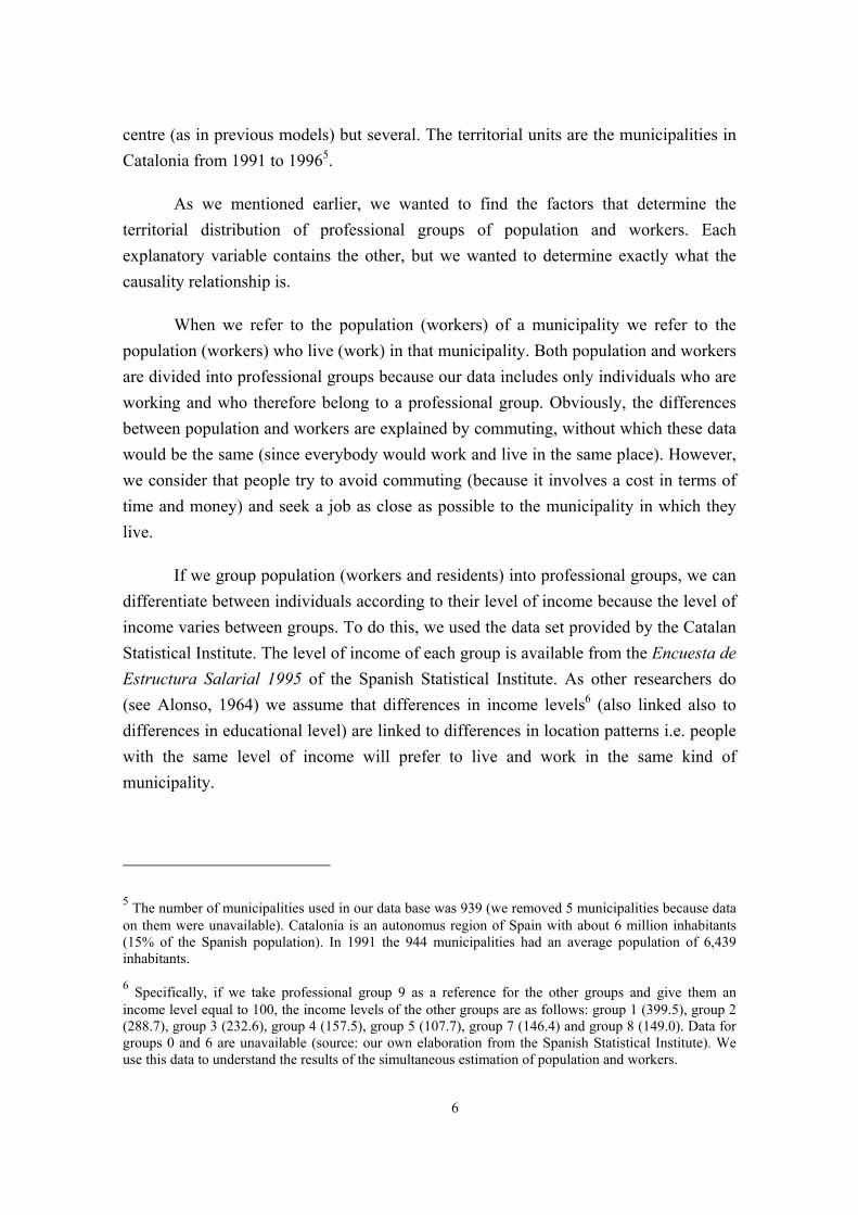
centre (as in previous models) but several. The territorial units are the municipalities in Catalonia from 1991 to 19965.

As we mentioned earlier, we wanted to find the factors that determine the territorial distribution of professional groups of population and workers. Each explanatory variable contains the other, but we wanted to determine exactly what the causality relationship is.

When we refer to the population (workers) of a municipality we refer to the population (workers) who live (work) in that municipality. Both population and workers are divided into professional groups because our data includes only individuals who are working and who therefore belong to a professional group. Obviously, the differences between population and workers are explained by commuting, without which these data would be the same (since everybody would work and live in the same place). However, we consider that people try to avoid commuting (because it involves a cost in terms of time and money) and seek a job as close as possible to the municipality in which they live.

If we group population (workers and residents) into professional groups, we can differentiate between individuals according to their level of income because the level of income varies between groups. To do this, we used the data set provided by the Catalan Statistical Institute. The level of income of each group is available from the Encuesta de Estructura Salarial 1995 of the Spanish Statistical Institute. As other researchers do (see Alonso, 1964) we assume that differences in income levels6 (also linked also to differences in educational level) are linked to differences in location patterns i.e. people with the same level of income will prefer to live and work in the same kind of municipality.

5 The number of municipalities used in our data base was 939 (we removed 5 municipalities because data on them were unavailable). Catalonia is an autonomus region of Spain with about 6 million inhabitants (15% of the Spanish population). In 1991 the 944 municipalities had an average population of 6,439 inhabitants.

6 Specifically, if we take professional group 9 as a reference for the other groups and give them an income level equal to 100, the income levels of the other groups are as follows: group 1 (399.5), group 2 (288.7), group 3 (232.6), group 4 (157.5), group 5 (107.7), group 7 (146.4) and group 8 (149.0). Data for groups 0 and 6 are unavailable (source: our own elaboration from the Spanish Statistical Institute). We use this data to understand the results of the simultaneous estimation of population and workers.

7

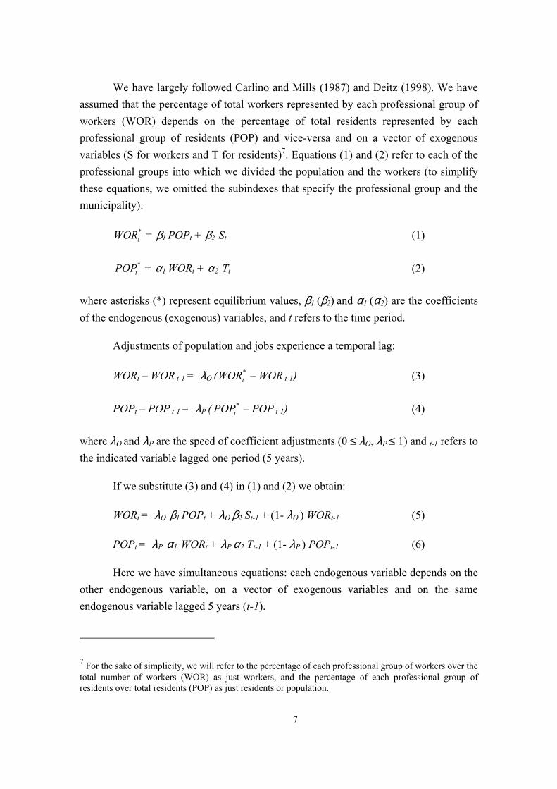
We have largely followed Carlino and Mills (1987) and Deitz (1998). We have assumed that the percentage of total workers represented by each professional group of workers (WOR) depends on the percentage of total residents represented by each professional group of residents (POP) and vice-versa and on a vector of exogenous variables (S for workers and T for residents)7. Equations (1) and (2) refer to each of the professional groups into which we divided the population and the workers (to simplify these equations, we omitted the subindexes that specify the professional group and the municipality):

*tWOR = β1 POPt + β2 St (1)

*tPOP = α1 WORt + α2 Tt (2)

where asterisks (*) represent equilibrium values, β1 (β2) and α1 (α2) are the coefficients of the endogenous (exogenous) variables, and t refers to the time period.

Adjustments of population and jobs experience a temporal lag:

WORt – WOR t-1 = λO ( *tWOR – WOR t-1) (3)

POPt – POP t-1 = λP ( *tPOP – POP t-1) (4)

where λO and λP are the speed of coefficient adjustments (0 ≤ λO, λP ≤ 1) and t-1 refers to the indicated variable lagged one period (5 years).

If we substitute (3) and (4) in (1) and (2) we obtain:

WORt = λO β1 POPt + λO β2 St-1 + (1- λO ) WORt-1 (5)

POPt = λP α1 WORt + λP α2 Tt-1 + (1- λP ) POPt-1 (6)

Here we have simultaneous equations: each endogenous variable depends on the other endogenous variable, on a vector of exogenous variables and on the same endogenous variable lagged 5 years (t-1).

7 For the sake of simplicity, we will refer to the percentage of each professional group of workers over the total number of workers (WOR) as just workers, and the percentage of each professional group of residents over total residents (POP) as just residents or population.

8

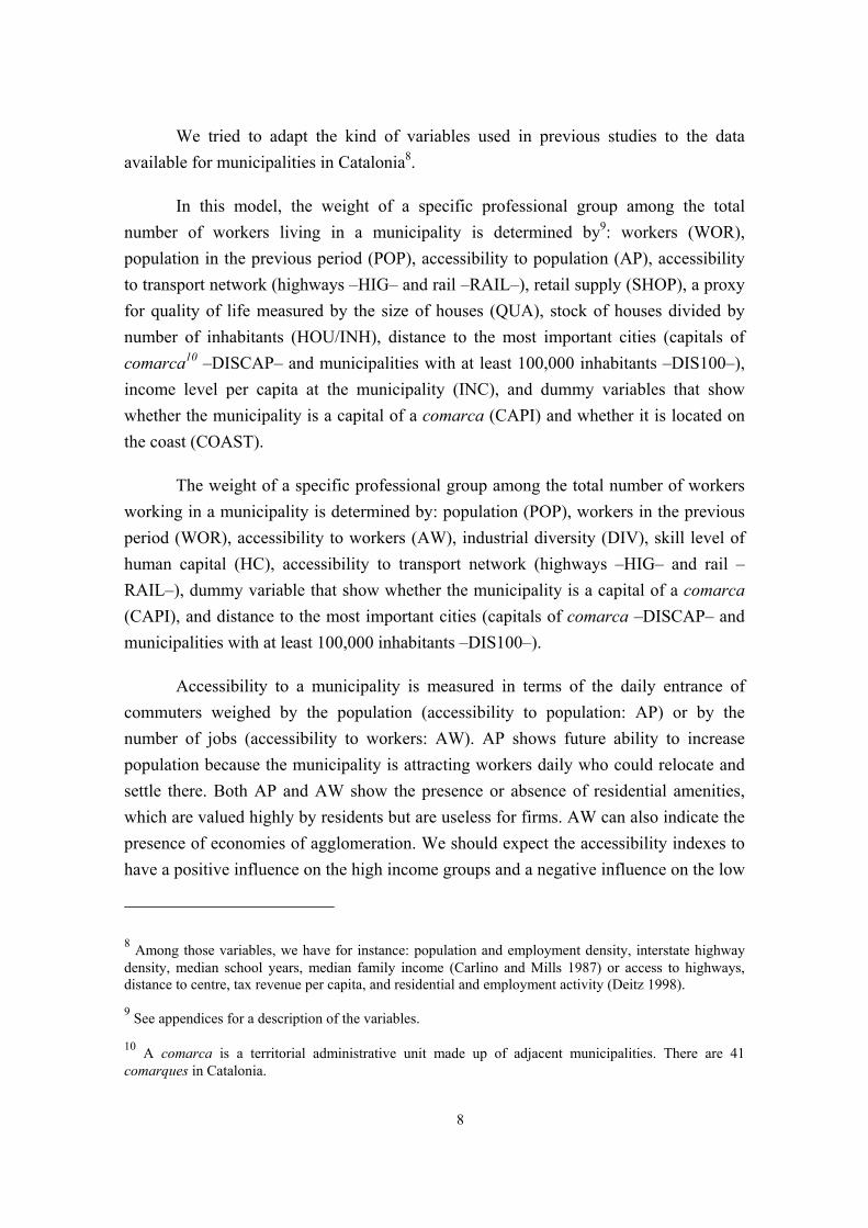
We tried to adapt the kind of variables used in previous studies to the data available for municipalities in Catalonia8.

In this model, the weight of a specific professional group among the total number of workers living in a municipality is determined by9: workers (WOR), population in the previous period (POP), accessibility to population (AP), accessibility to transport network (highways –HIG– and rail –RAIL–), retail supply (SHOP), a proxy for quality of life measured by the size of houses (QUA), stock of houses divided by number of inhabitants (HOU/INH), distance to the most important cities (capitals of comarca10 –DISCAP– and municipalities with at least 100,000 inhabitants –DIS100–), income level per capita at the municipality (INC), and dummy variables that show whether the municipality is a capital of a comarca (CAPI) and whether it is located on the coast (COAST).

The weight of a specific professional group among the total number of workers working in a municipality is determined by: population (POP), workers in the previous period (WOR), accessibility to workers (AW), industrial diversity (DIV), skill level of human capital (HC), accessibility to transport network (highways –HIG– and rail –RAIL–), dummy variable that show whether the municipality is a capital of a comarca (CAPI), and distance to the most important cities (capitals of comarca –DISCAP– and municipalities with at least 100,000 inhabitants –DIS100–).

Accessibility to a municipality is measured in terms of the daily entrance of commuters weighed by the population (accessibility to population: AP) or by the number of jobs (accessibility to workers: AW). AP shows future ability to increase population because the municipality is attracting workers daily who could relocate and settle there. Both AP and AW show the presence or absence of residential amenities, which are valued highly by residents but are useless for firms. AW can also indicate the presence of economies of agglomeration. We should expect the accessibility indexes to have a positive influence on the high income groups and a negative influence on the low

8 Among those variables, we have for instance: population and employment density, interstate highway density, median school years, median family income (Carlino and Mills 1987) or access to highways, distance to centre, tax revenue per capita, and residential and employment activity (Deitz 1998).

9 See appendices for a description of the variables.

10 A comarca is a territorial administrative unit made up of adjacent municipalities. There are 41 comarques in Catalonia.

9

income groups, mainly because high income groups prefer a low density environment and low income groups prefer a high density environment.

Accessibility to the railway and highway networks is based on the comarca to which each municipality belongs. This is a dummy variable that shows whether there is a railway or highway network in a comarca in which the municipality is located. Clearly, the accessibility to a transport network increases the attractiveness of the site for both jobs and population according to people's requirements for mobility. For instance, the higher the income, the greater the distance travelled every day, so the higher income groups, who usually use their own car, should depend more on the location of highways.

The distance from the most important cities (measured in terms of size or functions) is important because it is assumed that there are spillover effects that go beyond municipalities' administrative borders i.e. the greater the distance to the most dynamic cities, the smaller the influence of the activities that take place within them. We do not think that the need to be located near these centres is the same for all professional groups. For instance, higher income groups need to be located near larger cities because these have a wider variety of goods and services than the capitals of the comarques (which are smaller and have less retail variety).

Also from the geographical point of view, it is important whether the cities are located on the coast or a long way from it. Glaeser et al. (2001) showed that for counties in the United States between 1977 and 1995, proximity to the coast positively affected the growth of the population because this was considered a residential amenity.

According to the variables listed in (5) and (6), therefore, this system of equations is not strictly symmetrical, since all the independent variables of the first (second) equation do not appear as independent variables of the second (first) equation. What we do have is a collection of common variables, or at least a collection of highly likely variables.

As we mentioned earlier, the aim of this paper is to simultaneously determine the variables that affect residents and workers at a local level. We have used two equations because there are two endogenous variables (residents and workers) that are at the same time mutually explanatory. As this is a simultaneous equation model, the parameters of one equation cannot be estimated independently of the other, so we made the estimation of the system using two-stage least-squares (TSLS) method.

10

We chose this method because the relationship between the variables is bi-directional and so an OLS model would not provide consistent estimators. The specific problem is that the endogenous variables are correlated with the stochastic term of the equation in which they appear as explanatory variables. TSLS can therefore provide consistent and efficient estimators.

At a first stage we used instrumental variables that were not correlated with the random terms to calculate the values of the problematic variables. At a second stage we used these results to model linear regression for the dependent variable.

In this system of equations there was a correlation between the stochastical variable and the random term of the other equation i.e. WORi with ∈ i and POPi with vi. This means that an instrumental variable or proxy must be found for the stochastic explanatory variable WORi (POPi), so that this new variable correlates with WORi (POPi) but not with ∈ i (vi).

We first regressed the endogenous variables over all the exogenous variables (this eliminates the correlation between WORi (POPi) and ∈ i (vi)):

tiOiOiOOti TSWOR ,,210, ν+++= ∏∏∏ (7)

+++= ∏∏∏ TSPOP PiPPti 210, tiP ,,∈ (8)

where i refers to the municipality and t refers to the time period.

We then made the following transformation:

iOiOOti TSWOR ∏∏∏ ++=^

2

^

1

^

0, (9)

iPiPPti TSPOP ∏∏∏ ++=^

2

^

1

^

0, (10)

So that tiOtiti WORWOR ,,,, ν+= and tiPtiti POPPOP ,,,, ε+= .

At a second stage, we substituted WORi,t and POPi,t in the original equations and then regressed by OLS:

11

WORi,t = β1 t,iPOP t + β2 St-1 + *,tiν (11)

POPi,t = α1 t,iWOR + α2 Tt-1 + *,tiε (12)

where, *1,

*, Pttiti εβνν += and *

1,*, ˆOttiti ναεε += .

From the previously explained model, we now have the econometric specification to be estimated:

WORi,t = β1 POPi,t + β2 AOz,t-1 + β3 HIG + β4 RAIL +

+ β5 DIVt-1 + β6 CHt-1 +β7 CAP + β8 DISCAP + (13)

+ β9 DIS100 + β10 WORi,t-1 + vi,t

POPi,t = α1 WORi,t + α2 APz,t-1 + α3 SHOPz,t-1 + α4 HIG +

+ α5 RAIL +α6 HOU/INHt-1 + α7 INCt-1 +α8 QUA t-1 + (14)

+ α9 CAP + α10 COAST +α11 DISCAP + α12 DIS100 +

+α13 POPi,t-1 +∈ i,t

In this estimation, period t refers to 1996, period t-1 refers to 1991, and i refers to the municipality. We initially intended to lag variables by two periods (from 1986), not just one, but no data were available to link the data of 1986 with those of 1996.

To avoid problems caused by mixing larger and smaller municipalities, we have two possible solutions. The first one (Carlino and Mills 1987) involves the densities of the population and the workers . The second one (Deitz 1998) involves the percentages of each professional group in terms of the total population and the total number of workers.

Carlino and Mills' solution uses the density of the number of population and workers rather than the total number of population and workers (for each municipality we have: number of workers / km2). As we are using the area of the municipality (km2)

12

in other explanatory variables, however, this solution could cause multi-colineality problems. To avoid this, we chose Deitz' solution11.

4. Results

Table 1 shows the results of the simultaneous estimation of population and workers. Before interpreting the results, we need to remember that POPi and WORi refer to the percentage of a specific professional group in the total population in a municipality and the percentage of a specific professional group in the total number of jobs in a municipality, respectively. These data therefore provide information about the distribution of individuals between different groups but not about the intensity of land use.

Econometric estimations supported the "jobs follow people" hypothesis slightly more than they supported the "people follow jobs" hypothesis, but we should stress that there was an interaction between the two variables in the two possible directions. These results agree with those of Boarnet (1994), Steinnes (1977), Mills (1970), Muth (1968) or Deitz (1998). However, this is an analysis inside each professional group, not a comparison between one sector and all the residents or workers. Here we are analysing whether the location of population (workers) at sector i affects the location of workers (population) at professional group i. It is important to note that for some professional groups, the location of the job did not influence the location of the population (groups 2, 3 and 4), and vice-versa (group 8). This means that people in these groups have very different needs regarding their living and working environment. At the same time, the endogenous variable lagged also affected where residents and workers locate.

Another important conclusion is that people from different professional groups also have different location patterns and do not react in the same way to the same location variables. This could be because of the different income levels linked to each professional group.

11 At any rate, it may be that when working with professional groups, some crossed effects among these groups are not caught. However, we do not consider this problem to be so important for our overall results.

13

Table 1. Simultaneous estimations by professional categories

POPULATION 1996 POP96 1 POP96 2 POP96 3 POP96 4 POP96 5 POP96 6 POP96 7 POP96 8 POP96 9 POP96 0 CONS -2.8701

(1.0566)* -0.7697 (0.9620)

3.5688 (1.0511)*

1.0271 (0.4916)*

4.2808 (0.8807)*

4.1706 (1.5477)*

5.6331 (1.1193)*

11.0753 (1.3275)*

7.1256 (0.9102)*

0.0385 (0.0546)

WOR96 0.3180 (0.1155)*

-0.0957 (0.0719)

-0.0054 (0.0674)

0.35847 (0.13820)

0.1797 (0.0443)*

0.1106 (0.0293)*

0.2176 (0.0393)*

0.1450 (0.0334)*

0.3189 (0.0690)*

0.0314 (0.0133)*

POP91 0.2731 (0.0428)*

0.8154 (0.0371)*

0.5746 (0.0350)*

0.2722 (0.0543)*

0.3854 (0.0388)*

0.6125 (0.0307)*

0.4553 (0.0307)*

0.5815 (0.0312)*

0.2566 (0.0324)*

0.2356 (0.0220)*

INC 0.0021 (0.0003)*

0.0015 (0.0003)*

0.0021 (0.0004)*

0.0001 (0.0002)

-0.0001 (0.0003)

-0.0015 (0.0005)*

-0.0007 (0.0003)*

-0.0010 (0.0003)*

-0.0009 (0.0002)*

-0.0000 (0.0000)

SHOP -0.0062 (0.0053)

0.0067 (0.0053)

0.0037 (0.0054)

0.0043 (0.0026)**

0.0041 (0.0046)

-0.0069 (0.0080)

0.0007 (0.0053)

0.0015 (0.0066)

0.0057 (0.0044)

0.0000 (0.0003)

QUA 0.0163 (0.0060)*

0.0156 (0.0060)*

-0.0026 (0.0068)

-0.0025 (0.003)

-0.0089 (0.0054)

0.0054 (0.0010)

-0.0111 (0.0064)*

-0.0311 (0.0078)*

-0.0208 (0.0052)*

-0.0000 (0.0003)

HOU/INH 1.4403 (0.3193)*

0.8934 (0.2853)*

1.4190 (0.2946)*

0.1671 (0.1500)

0.7350 (0.2713)*

-2.7694 (0.4519)*

-0.2485 (0.2966)

-0.7338 (0.3733)*

-0.8538 (0.2458)*

0.0130 (0.0165)

CAP 0.0146 (0.5956)

0.2593 (0.6226)

0.1709 (0.6501)

0.0371 (0.3129)

0.4702 (0.5367)

-0.0091 (0.9210)

0.1922 (0.6061)

0.0577 (0.7447)

0.4963 (0.4944)

0.0124 (0.0342)

COAST 0.4643 (0.5216)

-0.7879 (0.4768)**

-0.6480 (0.4910)

-0.1458 (0.2548)

1.3792 (0.4716)*

2.1989 (0.7653)*

-0.6685 (0.5015)

-1.2977 (0.6274)*

0.8421 (0.4227)*

-0.0438 (0.0285)

DISCAP 3.98E-06 (0.0000)

2.42E-05 (1.01E-05)*

3.78E-06 (1.03E-05)

-3.58E-06 (5.08E-06)

-1.13E-05 (9.30E-06)

5.13E-06 (1.62E-05)

-1.25E-05 (1.07E-05)

-1.78E-05 (1.31E-05)

-4.89E-06 (8.72E-06)

-1.02E-06 (5.90E-07)**

DIS100 8.72E-06 (0.0000)

1.15E-05 (4.57E-06)*

-2.67E-05 (4.80E-06)*

4.72E-06 (2.34E-06)*

1.53E-05 (4.33E-06)*

-9.45E-06 (7.30E-06)

2.00E-05 (4.83E-06)*

-1.07E-05 (6.05E-06)**

-2.43E-06 (3.94E-06)

-3.03E-07 (2.72E-07)

AP 0.8585 (0.7854)

-1.2726 (0.6622)**

-0.3288 (0.8643)

1.0035 (0.3575)*

1.3169 (0.6053)*

0.0909 (1.1889)

-0.2712 (0.6736)

-0.2799 (1.0593)

1.1239 (0.5704)*

-0.0026 (0.0378)

HIG 0.1840 (0.2851)

0.4962 (0.2705)**

-0.0565 (0.2838)

0.2001 (0.1441)

0.6935 (0.2495)*

-0.8369 (0.4293)**

0.1209 (0.2819)

-0.7217 (0.3487)*

0.1868 (0.2349)

-0.0149 (0.0157)

RAIL -0.0007 (0.3733)

-0.0497 (0.3572)

-0.6257 (0.3731)**

0.3311 (0.1804)**

-0.1229 (0.3303)

0.8461 (0.5785)

-0.1649 (0.3738)

0.2674 (0.4658)

-0.2521 (0.3173)

0.0206 (0.0210)

Obs. 939 939 939 939 939 939 939 939 939 939 R2 0.6133 0.4614 0.5526 0.3423 0.5153 0.8819 0.6814 0.6858 0.3899 0.2829 F-Stat 48.90583* 65.84732* 88.1256* 19.14689* 59.96799* 514.6858* 130.3986* 143.5538* 26.93994* 27.23386*

WORKERS 1996 WOR96 1 WOR96 2 WOR96 3 WOR96 4 WOR96 5 WOR96 6 WOR96 7 WOR96 8 WOR96 9 WOR96 0 CONS 4.8779

(0.8655)* 3.0902

(0.6889)* 3.4175

(0.6370)* 0.4259

(0.3858) -1.1162 (0.9480)

4.0245 (1.3343)*

2.5583 (1.5130)**

4.3728 (1.2660)*

3.8014 (1.0168)*

0.0076 (0.0591)

POP96 0.3040 (0.0972)*

-0.1861 (0.0747)*

0.1714 (0.453)*

0.5908 (0.1232)*

0.4343 (0.0960)*

0.2699 (0.0535)*

0.3358 (0.0739)*

0.0422 (0.0604)

0.2245 (0.1156)**

-0.8648 (0.1804)*

WOR91 0.1975 (0.0447)*

0.6929 (0.0479)*

0.4822 (0.0283)*

0.2697 (0.0633)*

0.5970 (0.0453)*

0.5768 (0.0372)*

0.4533 (0.0334)*

0.7450 (0.0342)*

0.3086 (0.0463)*

0.7931 (0.0215)*

HC 0.0999 (0.0842)

0.3993 (0.0934)*

-0.1901 (0.0466)*

0.0690 (0.0239)*

0.1774 (0.0542)*

0.0686 (0.1010)

0.0933 (0.0745)

-0.3608 (0.0798)*

0.1316 (0.0550)*

-0.0034 (0.0045)

DIV -4.0342 (1.0362)*

-1.0392 (0.7452)

-4.7508 (0.6459)*

-0.4577 (0.38165)

-0.2036 (0.9400)

8.9607 (3.0939)*

-2.5243 (1.3649)**

-0.8507 (1.1450)

-3.7354 (0.7595)*

0.2147 (0.0697)*

CAP -0.5202 (0.7808)

1.7581 (0.5790)*

3.1726 (0.5021)*

0.5227 (0.3172)

0.5558 (0.6588)

-2.2340 (1.2736)**

-2.5408 (0.8262)*

0.1143 (0.8754)

-0.3889 (0.5552)

-0.0816 (0.0602)

DISCAP 0.0000 (0.0000)

1.69E-05 (1.00E-05)**

1.95E-05 (8.56E-06)*

1.15E-06 (5.49E-06)

1.46E-05 (1.17E-05)

-4.30E-05 (2.25E-05)**

-1.53E-05 (1.48E-05)

-1.02E-05 (1.56E-05)

1.09E-05 (9.53E-06)

-3.06E-06 (1.05E-06)*

DIS100 0.0000 (0.0000)*

-8.96E-07 (4.47E-06)

-7.74E-06 (4.06E-06)**

-6.26E-06 (2.47E-06)*

2.04E-06 (5.71E-06)

-9.35E-06 (9.99E-06)

1.48E-05 (6.74E-06)*

-4.14E-06 (7.14E-06)

-3.55E-09 (4.28E-06)

-1.12E-06 (4.68E-07)*

AW -2.4770 (0.6188)*

0.0349 (0.4409)

3.2312 (0.4099)*

0.2760 (0.2725)

0.2779 (0.5105)

-8.0754 (1.0194)*

-1.2486 (0.6569)**

6.8432 (0.7000)*

1.0202 (0.4174)*

0.0896 (0.0459)**

HIG 0.4535 (0.3713)

0.4378 (0.2671)

0.3259 (0.2323)

0.2043 (0.1537)

-0.0645 (0.3315)

-0.1608 (0.6004)

-0.3665 (0.3961)

-1.0013 (0.4212)*

0.1494 (0.2547)

0.0088 (0.0278)

RAIL 0.3084 (0.4907)

0.1622 (0.3524)

-0.3608 (0.3024)

-0.2876 (0.1957)

-0.1493 (0.4101)

-0.052 (0.7927)

1.1740 (0.5202)*

-0.0217 (0.5496)

-0.5174 (0.3395)

-0.0213 (0.0373)

Obs. 939 939 939 939 939 939 939 939 939 939 R2 0.4361 0.2809 0.7013 0.3597 0.6131 0.8944 0.6490 0.7555 0.3853 0.7916 F-Stat 21.63808* 50.38677* 206.4024* 29.5793* 119.6628* 759.5041* 147.3889* 283.1894* 41.10404* 385.8058*

(*) Significance at 5% and (**) significance at 10%. Standard errors in brackets.

14

We can analyse both sides of the interaction between location patterns of workers and residents. On the one hand, in 9 of the 10 groups12 the location of workers was affected by the location of residents. In 7 groups, this was positive (company directors; technicians and support professionals; administrative staff; retail and restaurant staff; qualified workers in the farming and fishing industries; manufacturing, construction and mining workers; and non-qualified workers) and in 2 groups, it was negative (technicians, scientists and intellectual professionals; and the army).

On the other hand, in 7 of the 10 groups13 the location of residents was affected by the location of workers, and in all groups there was a positive influence (company directors; retail and restaurant staff; qualified workers in the farming and fishing industries; manufacturing, construction and mining workers; operators of facilities and machinery; non-qualified workers; and the army).

In any case, we should be aware that we have used aggregated data at a local level, which means that some elements of wasteful commuting may be hidden inside these data14.

One of the variables that influence the location of residents is the municipality’s mean fiscal income (INC). As it is obvious, in municipalities with many people of high income (groups 1, 2 and 3), there are also high mean income levels, and in municipalities with many people of low incomes (groups 6, 7, 8 and 9) there are low mean income levels. The variable for the average area of houses (QUA) can be analysed in a similar way: a positive reaction from higher income groups (1 and 2) and a negative reaction from smaller income groups (7, 8 and 9). The variable for the stock of houses divided by number of inhabitants (HOU/INH) can also be analysed in this way: a positive reaction from higher income groups (1, 2 and 3) and a negative reaction from smaller income groups (6, 8 and 9).

12 About 84.32% of the workers.

13 About 64.41% of the residents.

14 Wasteful commuting means that some commuting between two sites is unnecessary. Imagine, for instance, that two individuals living in municipalities “a” and “b”, respectively, are working in the municipalities “b” and “a”, respectively, and commute daily between the two sites. See Hamilton for a more detailed explanation (1982 and 1989).

15

We tried to measure the influence of amenities by considering the municipalities that are capitals of a comarca. However, the lack of significance of this variable could be due to the heterogeneity of these municipalities15 and the fact there is not always a relationship between the capital of a comarca and a large level of economic activity. Another reason could be the increasing urban sprawl, which benefits smaller cities. We could explain the variable that measures the distance from the capital of the comarca (DISCAP) in a similar way.

Accessibility to the population (AP) is a significant variable in only 4 of the 10 estimates. A positive sign (groups 4, 5 and 9) implies that the weight of the resident population in each professional group benefits from a higher number of past entrants (in comparison to total population). This could be because these groups prefer to be located close to the places where jobs are located16. A negative sign (group 2) indicates that the residential population of this professional group reacts negatively to the high entrance of workers. The explanation for this is similar to the previous one: as group 2 is made up of people with high incomes, it is reasonable to suppose that they prefer low-density environments.

Some professional groups react positively to the presence of skilled human capital (groups 2, 4, 5 and 9), while others react negatively (groups 3 and 8). A close relationship among higher skilled groups (1, 2 and 3) and municipalities with more skilled people is logical, but we should remember that these groups tend to commute more (Casado, 2000).

All groups except those with highly specific location patterns (i.e. qualified workers in the farming and fishing industries and the army) prefer a diversified industrial environment.

Although it was not true for the residential population, being in a capital of a comarca is significant for some groups of workers . This is positive for two of the

15 For instance, besides capitals of comarca like Barcelona (1,643,542 inhabitants in 1991) or Reus (87,670), there are others such as Falset (2,603) or Cervera (6,545).

16 These preferences could be due to a desire to reduce commuting costs or to the fact that the kind of urban environment in which these professional activities take place is very similar to a residential environment. We should note that with these accessibility indexes we are only talking about the total number of workers: we are not disaggregating them into professional groups. The main issue here is that a municipality can focus on a residential function or on a working function and that, depending on the professional group of the individuals, it prefers one of both of these environments.

16

higher-income groups (2 and 3) and negative for two of the smaller-income groups (6 and 7).

The results for accessibility to the workforce (AW) depended on the professional group: there was a positive effect on 3 groups and a negative effect on 4 groups.

Finally, the poor results for the variable for transport infrastructure (RAIL and HIG) show that there may not be a close relationship between these networks and the distribution of economic activity: it seems that firms choose other ways to transport their goods (toll-less highways, for instance).

We should explain what the differences in the values of R2 mean (in our results, R2 ranged from 0.27 to 0.85). A low R2 may be due to a non-linear relationship between variables or to important variables possibly omitted in our specification. This second possibility also implies that using a common specification for all the professional groups may not be the best idea because the variables that explain location patterns are not the same for all groups. If this is true, future research in this field should aim to identify the specific location determinants of each professional group.

5. Conclusions

We can summarise our main conclusions as follows:

Firstly, the location of population influences the location of jobs (grouped according to profession), and vice-versa, but the evidence that the location of population influences the location of jobs is stronger than the evidence that the location of jobs influences the location of population.

Secondly, location patterns depend on professional groups. The characteristics of the municipalities affect the kind of people and firms that locate there.

Thirdly, in most professional groups, workers (residents) from the same professional group influence residents (workers) in a positive way (although there is also evidence of a negative effect). This means that people prefer to live (work) in the same place as where they work (live), which is consistent with the low levels of commuting in Catalan municipalities compared to those of other countries. Clearly, as we do not have individual data, we ought to consider the possibility of reverse

17

commuting, which could hide preferences for living in a place that is different to where the job is located. However, we do not think that this is relevant in this case. At any rate, the differences between groups show that one's attitude to living and working in the same municipality depends on one's level of income, as does one's willingness to commute. Therefore, people's preferences are not neutral to their level of income.

Fourthly, the results of the different professional groups show some common patterns between them in terms of their income level.

Fifthly, the location patterns of residents and workers are different (residents, for example, prefer dispersion more than workers do).

Sixthly, the variables for transport infrastructure are less significant, perhaps because we did not select the most suitable ones. This result is reasonable if we consider that our data base contains more than 900 municipalities of very different sizes and that these have access to very different transport infrastructures.

These results can be used to draw up guidelines for policy makers. Territorial environments differ according to their allegiance to certain professional categories. The policies of local governments must therefore reflect the distribution of their residents and workers and, in particular, their strategic targets for each municipality. This means that they must choose whether to attract population and/or workers from certain professional groups.

Our future research in this field should focus on the size of the municipalities and determine whether, as we expect, the results of this paper are affected by it. At the moment we suspect that the determinants of location are not the same for large and small municipalities.

18

References

ALONSO, W. (1964) Location and Land Use. Cambridge: Harvard University Press.

BLANCO, C. (1963) The Determinants of Interstate Population Movements, Journal of Regional Science, 5, pp. 77-84.

BOARNET, M. (1994) The Monocentric Model and Employment Location, Journal of Urban Economics, 36, pp. 79-97.

CARLINO, G. A. and MILLS, E. S. (1987) The Determinants of County Growth, Journal of Regional Science, 27 (1), pp. 39-53.

CASADO, J. M. (2000) Local Labour Market Areas in Spain: a Case Study, Regional Studies, 34 (9), pp. 843-856.

DEITZ, R. (1998) A Joint Model of Residential and Employment Location in Urban Areas, Journal of Urban Economics, 44, pp. 197-215.

GARREAU, J. (1991) Edge City: Life on the New Frontier. New York: Doubleday.

GLAESER, E. L.; KOLKO, J. and SAIZ, A. (2001) Consumer City, Journal of Economic Geography, 1, pp. 27-50.

HAMILTON, B. W. (1989) Wasteful Commuting Again, Journal of Political Economy, 97 (6), pp. 1497-1504.

HAMILTON, B. W. (1982) Wasteful Commuting, Journal of Political Economy, 90 (5), pp. 1035-1053.

KAIN, J. F. (1968) The Distribution and Movement of Jobs and Industry, in J. Wilson (ed.), The Metropolitan Enigma, pp. 1-42. Cambridge: Harvard University Press.

LOWRY, I. S. (1966) Migration and Metropolitan Growth: Two Analytical Models. San Francisco: Chandler.

MILLS, E. S. (1986) Metropolitan Central City Population and Employment Growth during the 1970s, in M. H. Peston and R. E. Ivandt, Prices, Competition and Equilibrium, pp. 268-284. London: Philip Allan Publishers.

MILLS, E. S. and PRICE, R. (1984) Metropolitan Suburbanization and Central City Problems, Journal of Urban Economics, 15 (1), pp. 1-17.

MUTH, R. F. (1968) Differential Growth Among Large U.S. Cities, in J.P. Quirk and A.M. Zarley (eds.), Papers in Quantitative Economics. Lawrence: The University of Kansas.

OFFICE OF POLICY DEVELOPMENT AND RESEARCH (1995) The Clinton Administration’s National Urban Policy Report, U.S. Department of Housing and Urban Development.

19

SIMPSON, W. (1987) Workplace Location, Residential Location and Urban Commuting, Urban Studies, 24, pp. 119-128.

STEINNES, D. (1982) Do ‘people follow jobs’ or do ‘jobs follow people’? A Causality Issue in Urban Economics, Urban Studies, 19, pp. 187-192.

STEINNES, D. (1978) A Simultaneous Econometric Model of the Intra-urban Location of Employment and Residence, Regional Science Perspectives, 8, pp. 101-115.

STEINNES, D. (1977) Causality and Intraurban Location, Journal of Urban Economics, 4, pp. 69-79.

STEINNES, D. and FISHER, W. (1974) An Econometric Model of Intraurban Location, Journal of Regional Science, 14 (1), pp. 65-80.

20

Appendices

Table A.1. Professional groups

Group code Description 1 Company directors 2 Technicians, scientists and intellectual professionals 3 Technicians and support professionals 4 Administrative staff 5 Retail and restaurant staff 6 Qualified workers in the farming and fishing industries 7 Manufacturing, construction and mining workers 8 Operators of facilities and machinery 9 Non-qualified workers 0 Armed forces

Source: Catalan Statistical Institute (IDESCAT).

21

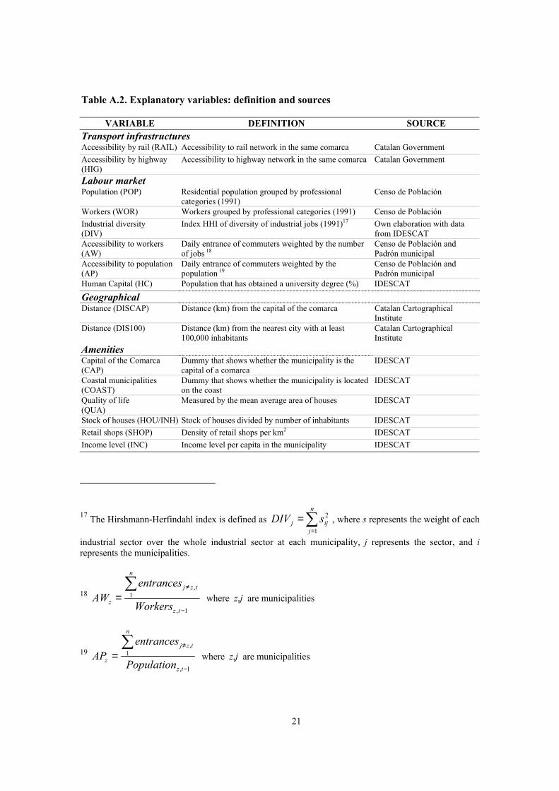
Table A.2. Explanatory variables: definition and sources

VARIABLE DEFINITION SOURCE Transport infrastructures Accessibility by rail (RAIL) Accessibility to rail network in the same comarca Catalan Government Accessibility by highway (HIG)

Accessibility to highway network in the same comarca Catalan Government

Labour market Population (POP) Residential population grouped by professional

categories (1991) Censo de Población

Workers (WOR) Workers grouped by professional categories (1991) Censo de Población Industrial diversity (DIV)

Index HHI of diversity of industrial jobs (1991)17 Own elaboration with data from IDESCAT

Accessibility to workers (AW)

Daily entrance of commuters weighted by the number of jobs 18

Censo de Población and Padrón municipal

Accessibility to population (AP)

Daily entrance of commuters weighted by the population 19

Censo de Población and Padrón municipal

Human Capital (HC) Population that has obtained a university degree (%) IDESCAT

Geographical Distance (DISCAP) Distance (km) from the capital of the comarca Catalan Cartographical

Institute Distance (DIS100) Distance (km) from the nearest city with at least

100,000 inhabitants Catalan Cartographical Institute

Amenities Capital of the Comarca (CAP)

Dummy that shows whether the municipality is the capital of a comarca

IDESCAT

Coastal municipalities (COAST)

Dummy that shows whether the municipality is located on the coast

IDESCAT

Quality of life (QUA)

Measured by the mean average area of houses IDESCAT

Stock of houses (HOU/INH) Stock of houses divided by number of inhabitants IDESCAT Retail shops (SHOP) Density of retail shops per km2 IDESCAT Income level (INC) Income level per capita in the municipality IDESCAT

17 The Hirshmann-Herfindahl index is defined as ∑=

=n

jijj sDIV

1

2 , where s represents the weight of each

industrial sector over the whole industrial sector at each municipality, j represents the sector, and i represents the municipalities.

18 1,

1,

−

≠∑=

tz

n

tzj

z Workers

entrancesAW where z,j are municipalities

19 1,

1,

−

≠∑=

tz

n

tzj

z Population

entrancesAP where z,j are municipalities