determinants of foreign direct...
TRANSCRIPT

Determinants of foreign direct investment
Bruce A. Blonigen University of OregonJeremy Piger University of Oregon
Abstract. Empirical studies of bilateral foreign direct investment (FDI) activity showsubstantial differences in specifications with little agreement on the set of included co-variates. We use Bayesian statistical techniques that allow one to select from a large set ofcandidates those variables most likely to be determinants of FDI activity. The variableswith consistently high inclusion probabilities include traditional gravity variables, culturaldistance factors, relative labour endowments and trade agreements. There is little supportfor multilateral trade openness, most host-country business costs, host-country infras-tructure and host-country institutions. Our results suggest that many covariates foundsignificant by previous studies are not robust.
Resume. Les determinants de l’investissement direct a l’etranger. Les etudes empiriquesdes determinants des activites d’investissement direct bilateral a l’etranger ont desspecifications substantiellement differentes et peu d’accord sur les variables co-relieesincluses. On utilise des techniques statistiques bayesiennes qui permettent de balayer unvaste ensemble de variables a la recherche de celles qui sont davantage susceptibles d’etredes determinants des activites d’investissement direct a l’etranger. Les variables qui seretrouvent de maniere reguliere dans la liste de haute probabilite d’impact sont les vari-ables reliees a la gravite, les facteurs lies a la distance culturelle, les dotations relatives enfacteur travail, et les accords commerciaux. Il y a peu de support pour des variables commel’ouverture au commerce multilateral, la plupart des couts d’affaires, les infrastructureset les institutions dans les pays hotes. Ces resultats suggerent que plusieurs co-variationsqu’on a jugees significatives dans les etudes anterieures ne sont pas robustes.
JEL classification: F21, F23, C52
1. Introduction
Empirical analyses of the factors determining foreign direct investment (FDI)across countries have employed a variety of econometric specifications. Manyprevious studies of cross-country FDI activity have used a gravity equation,which controls mainly for the economic size of the parent and host countries, the
We thank Theo Eicher, Gordon Hanson, Kathryn Russ, Deborah Swenson, anonymous refereesand session participants at a Western Economic Association session for helpful comments.Blonigen is also a research associate of the National Bureau of Economic Research. Any errorsor omissions are completely our own.Corresponding author: J. Piger, [email protected]
Canadian Journal of Economics/Revue canadienne d’economique, Vol. 47, No. 3August 2014. Printed in Canada / Aout 2014. Imprime au Canada
0008-4085 / 14 / 775–812 / C© Canadian Economics Association
776 B. A. Blonigen and J. Piger
geographic distance separating the countries and proxies for certain economicfrictions. Like trade flows, this specification does a reasonably good job of fittingthe observed data, but leaves one wondering if such a parsimonious specificationcaptures all relevant factors.
Recent papers by Carr, Markusen and Maskus (2001; CMM) and Bergstrandand Egger (2007) have developed theoretical models of multinational enterprise’s(MNE’s) foreign investment decisions that suggest additional possible factors thatdetermine FDI patterns. These studies point out a number of modifications to astandard gravity model that may be necessary to accurately explain FDI patterns.First, while gravity variables may adequately capture “horizontal” motivationsfor FDI, where firms look to replicate their operations in other countries to bemore proximate to consumers in those markets, additional controls are necessaryto allow for “vertical” motivations of FDI, where firms look for low-cost locationsfor labour-intensive production. For example, these studies introduce measuresof relative labour endowments in the host country with the expectation thatcountries with relatively high shares of unskilled labour will be attractive locationsfor MNEs due to lower wages. In addition, these studies show that FDI decisionsby MNEs are complex enough that interactions between key variables (e.g.,GDP and skilled labour endowments) may be necessary to account for nonlineareffects of these variables on FDI patterns. Head and Ries (2008) differs fromthese previous studies by modelling FDI as arising from decisions by firms toacquire and control foreign assets (i.e., cross-border mergers and acquisitions),rather than development of new (or greenfield) plants. Their analysis of FDIpatterns highlights the potential role of common culture and language betweencountries.
While these prior studies have been important in deepening our understandingof the factors that determine cross-country FDI patterns, they have generallyfocused on regression models involving specific sets of covariates determined bythe researcher and the particular theoretical framework for FDI they chose toexamine. By conditioning on a particular regression model specification, thispractice ignores uncertainty regarding the model specification itself, which canhave dramatic consequences on inference.1 Most notably, inference regarding theeffects of included covariates can depend critically on what other covariates areincluded versus excluded.
In this paper, we take a Bayesian approach to confront uncertainty regardingthe appropriate set of covariates to include in a regression model explainingFDI activity. From a Bayesian perspective, incorporating such uncertainty isconceptually straightforward. The choice of covariates, or “model,” is treated asan additional parameter that lies in the space of potential models, which allows usto compute the posterior probability that each potential model is the true modelthat generated the data. Posterior distributions for objects of interest, such as
1 For discussion and examples, see Leamer 1978, Hodges 1987, Moulton 1991, Draper 1995,Kass and Raftery 1995, Raftery 1996 and Fernandez, Ley and Steel 2001a.

Determinants of foreign direct investment 777
the effect of a particular covariate, are then averaged across alternative models,using the posterior model probabilities as weights. This procedure, known asBayesian Model Averaging (BMA), produces inferences that are not conditionedon a particular model.
To be clear, we are taking a purely empirical approach to determine thecorrelates with observed FDI patterns. As we discuss in the next section, thereis very little consistency in the empirical FDI literature about the covariates oneshould use when empirically modeling cross-country FDI. We view this paper asa first step in pointing out these inconsistencies and providing evidence of theempirically robust determinants of FDI.
Although conceptually straightforward, BMA is practically difficult when theset of possible models is large, as direct calculation of posterior probabilities forall models becomes infeasible. In our application, we have a large set of potentialcovariates, which yields an extremely large set of possible models (> 7 × 10¹⁶).To sidestep this difficulty, we use techniques designed to obtain random draws ofmodels from the probability distribution defined by the posterior model probabil-ities. Such draws are made possible even when the posterior model probabilitiesare unknown by using the MC3 algorithm of Madigan and York (1995). Theserandom model draws are then used to construct estimates of the posterior modelprobabilities.2
Our set of potential FDI determinants is meant to be comprehensive andincludes a combination of covariates proposed by the previously mentionedstudies, as well as other prior literature on FDI. We examine mainly cross-sectional patterns for the year 2000.2 We examine both levels and log-linearregressions, placing more weight on our results for the log-linear regressionsbecause most previous studies have used a logarithmic transformation to addressskewness in the FDI variable. We also examine three measures of FDI—FDIstock, affiliate sales and cross-border mergers and acquisitions activity—in orderto better compare with a broader set of prior studies. At the end, we also explorea specification that first differences observations across the years 1990 and 2000to control for bilateral country-pair fixed effects as well as a negative binomialspecification to better model the nature of our dependent variable.
Our analysis indicates that many of the covariates used in prior FDI studies(and often found statistically significant) do not have a high probability of in-clusion in the true FDI determinants model once we consider a comprehensiveset of potential determinants using BMA. A fairly parsimonious set of covari-ates is suggested by our analysis. The covariates with consistently high inclusionprobabilities include traditional gravity variables, cultural distance factors, rela-tive labour endowments and trade agreements. Variables with little support forinclusion are multilateral trade openness, most host-country business costs, host-country infrastructure (including credit markets) and host-country institutions.
2 Focusing on the year 2000 maximized our available sample size by allowing us to use datasetsthat have not been updated recently along with datasets that began being collected in 2000.
778 B. A. Blonigen and J. Piger
A few variables that have rarely been included in prior FDI studies, namelyhost-country remoteness, parent-country real GDP per capita and host is anoil-exporting country, have surprisingly high inclusion probabilities.
The remainder of the paper proceeds as follows. The next section reviewsprevious empirical literature on the determinants of FDI and makes the casethat the appropriate model specification for explaining FDI patterns is far fromsettled. Section 3 then lays out the BMA methodology we use to assess modeluncertainty. Section 4 describes the data and its sources, while section 5 reportsthe results and compares to the existing literature. Section 6 concludes.
2. Prior FDI literature
There is little consensus on how to empirically model bilateral FDI patterns,with many past empirical FDI papers using a base model consisting of gravity-type covariates (country-level GDP and distance) because of its popularity forexplaining trade flows. As mentioned in the introduction, there have been a fewrecent efforts to develop specifications based on theoretical models—namely theknowledge-capital (K-K) model developed by James Markusen and co-authors,which was brought to data in CMM (2001), Bergstrand and Egger’s (2007) modelincorporating physical capital and Head and Ries’ (2008) model of acquisitionFDI.
There is little consistency in the covariates that are postulated to explain world-wide FDI patterns across these three papers. To see this, the first three columnsof table 1 lists the covariates used in each of these papers. Distance betweencountries is the only covariate common to all three studies. There are 22 differentcovariates between the three studies, even though each study averages only about10 covariates. While all three specifications postulate a role for economic sizeand trade frictions as driving forces of FDI, it is surprising how differently theyconstruct and define variables meant to proxy for these common factors.
Of course, there have been many other papers that have empirically examinedFDI patterns using specifications that differ from these three papers. Columns 4through 8 of table 1 list the covariates used in a number of other highly regardedrecent papers. Across these eight studies in columns 1 through 8, there are acombined 47 covariates. However, no covariate is shared by all eight studies and,on average, a covariate is used in only 1.7 of the eight studies. Interestingly, almost85% of the covariates included in these 8 studies are found to be statisticallysignificant. Given that the average study includes very few of the total set ofpossible covariates, the possibility of spurious correlations is quite real.
In addition to the substantial differences in covariates used across FDI studies,there are also differences across studies in whether variables are logged or whetherpanel data were used (these are noted in the first few rows of table 1). Given thesewide differences in specifications, there clearly is no consensus on how to specifythe determinants of bilateral FDI patterns.

Determinants of foreign direct investment 779
TA
BL
E1
Spec
ifica
tion
sof
prio
rst
udie
sof
FD
Ide
term
inan
ts
Car
r,B
ergs
tran
dH
ead
Mar
kuse
n,an
dan
dR
ies
Eat
onan
dW
eidi
Gio
vann
iSt
ein
and
Cha
krab
arti
Mas
kus
(200
1)E
gger
(200
7)(2
008)
Tam
ura
(199
4)(2
000)
(200
5)D
aude
(200
7)(2
001)
Dat
aan
dsp
ecifi
cati
ons
Dep
ende
ntva
riab
leSa
les
Sale
sSt
ock
and
M&
ASt
ock
Stoc
kM
&A
Stoc
kF
low
s
Var
iabl
eslo
gged
No
Yes
Yes
Yes
Yes
Yes
Som
eN
oP
anel
data
Yes
Yes
No
Yes
Yes
Yes
No
No
Tw
o-w
ayor
one-
way
flow
sT
wo-
way
Tw
o-w
ayT
wo-
way
Tw
o-w
ayO
ne-w
ayT
wo-
way
Tw
o-w
ayO
ne-w
ayG
ravi
tym
easu
res
PAR
EN
TG
DP
xx
HO
STG
DP
zx
xx
Dis
tanc
ez
xx
xx
xO
ther
GD
P-r
elat
edte
rms
PAR
EN
Tpe
rca
pita
GD
Px
HO
STpe
rca
pita
GD
Px
xx
PAR
EN
Tpo
pula
tion
xH
OST
popu
lati
onx
xx
GD
Psi
mila
rity
xG
DP
sum
xx
xG
DP
diff
eren
cex
GD
Ppe
rca
pita
diff
eren
ces
xx
HO
STG
DP
grow
thz
Res
t-of
-the
-wor
ldG
DP
xO
ther
geog
raph
ym
easu
res
Con
tigu
ous
bord
erz
Tim
ezo
nedi
ffer
ence
sx
Cou
ntry
-lev
elen
dow
men
tsR
elat
ive
skill
ed-u
nski
lled
labo
uren
dow
men
ts(s
kill
diff
eren
ce)
xx
x
Inte
ract
ion
ofsk
illdi
ffer
ence
san
dG
DP
diff
eren
ces
x
(Con
tinu
ed)

780 B. A. Blonigen and J. Piger
TA
BL
E1
(Con
tinu
ed)
Car
r,B
ergs
tran
dH
ead
Mar
kuse
n,an
dan
dR
ies
Eat
onan
dW
eidi
Gio
vann
iSt
ein
and
Cha
krab
arti
Mas
kus
(200
1)E
gger
(200
7)(2
008)
Tam
ura
(199
4)(2
000)
(200
5)D
aude
(200
7)(2
001)
Rel
ativ
eca
pita
l-la
bour
endo
wm
ents
x
HO
STw
ages
xz
HO
STpo
pula
tion
dens
ity
xH
OST
educ
atio
nle
vels
xB
ilate
ralc
ultu
rala
ndco
loni
allin
kage
sC
omm
onla
ngua
gex
xx
xz
Col
onia
llin
ksx
xM
ulti
late
ralt
rade
open
ness
HO
STtr
ade
cost
sx
zPA
RE
NT
trad
eco
sts
xH
OST
trad
eop
enne
ss(i
mpo
rts
plus
expo
rts
divi
ded
byG
DP
)
z
HO
STtr
ade
cost
sti
mes
skill
diff
eren
cete
rmsq
uare
dx
Bila
tera
ltra
deop
enne
ssB
ILA
TE
RA
Ltr
ansp
ort
cost
sz
BIL
AT
ER
AL
trad
eflo
ws/
defic
itx
z
Reg
iona
ltra
deag
reem
ent
xz
zC
usto
ms
unio
nz
Com
mon
serv
ice
sect
orag
reem
ent
x
Hos
tco
untr
yF
DI/
busi
ness
cost
sH
OST
FD
Ico
sts
xx
HO
STta
xes
xz
(Con
tinu
ed)

Determinants of foreign direct investment 781
TA
BL
E1
(Con
tinu
ed)
Car
r,B
ergs
tran
dH
ead
Mar
kuse
n,an
dan
dR
ies
Eat
onan
dW
eidi
Gio
vann
iSt
ein
and
Cha
krab
arti
Mas
kus
(200
1)E
gger
(200
7)(2
008)
Tam
ura
(199
4)(2
000)
(200
5)D
aude
(200
7)(2
001)
PAR
EN
Tta
xes
xPA
RE
NT
coun
try
has
tax
cred
itsy
stem
z
Cha
nge
inH
OST
cons
umer
pric
esz
Bila
tera
ltax
and
inve
stm
ent
agre
emen
tsT
axtr
eaty
xx
Inve
stm
ent
trea
tyz
Hos
tco
untr
yco
mm
unic
atio
nsin
fras
truc
ture
Tel
epho
netr
affic
xx
Hos
tco
untr
yfin
anci
alin
fras
truc
ture
HO
STm
arke
tca
pita
lizat
ion
xH
OST
dom
esti
ccr
edit
xPo
litic
alen
viro
nmen
tan
din
stit
utio
nsH
OST
polit
ical
stab
ility
xz
HO
STle
gali
nsti
tuti
ons
xH
OST
corr
upti
onx
Exc
hang
era
tes
Exc
hang
era
tes
zz
Vol
atili
tyof
exch
ange
rate
sx
NO
TE
S:A
n“x
”si
gnifi
esth
ata
vari
able
isin
clud
edan
dst
atis
tica
llysi
gnifi
cant
inth
em
ajor
ity
ofsp
ecifi
cati
ons
repo
rted
inth
epa
per.
A“z
”si
gnifi
esth
ata
vari
able
isin
clud
ed,b
utit
isno
tst
atis
tica
llysi
gnifi
cant
inth
em
ajor
ity
ofsp
ecifi
cati
ons
repo
rted
inth
epa
per.
We
excl
ude
from
this
tabl
eva
riab
les
that
Cha
krab
arti
(200
1)po
site
das
exan
tedo
ubtf
ulan
dth
atdi
dno
tco
me
inst
atis
tica
llysi
gnifi
cant
inth
atan
alys
is.T
hety
peof
depe
nden
tva
riab
lein
thes
est
udie
sva
ried
inco
nstr
ucti
onbu
tca
nbe
char
acte
rize
dby
data
onaf
filia
tesa
les,
whi
chw
ete
rmS
ales
inth
eta
ble;
FD
Ist
ock,
Sto
ck;F
DI
flow
s,Fl
ows;
and/
orco
unts
(or
valu
e)of
cros
s-bo
rder
mer
gers
and
acqu
isit
ions
acti
vity
,M&
A.

782 B. A. Blonigen and J. Piger
The final paper documented in table 1 (last column) is Chakrabarti (2001).This paper is similar to ours in its motivation to understand which covariatesare more likely to be robust determinants of bilateral FDI. However, the analysisconsiders a surprisingly small set of possible covariates, perhaps because it camebefore some of the recent advances in the literature. Also, it follows a differentmethodology (extreme bounds analysis) from ours, feasible implementation ofwhich requires the model space be restricted a priori. The approach we taketo implement BMA requires no such restriction and is designed to identify andexplore relevant portions of the entire model space. That said, Chakrabarti (2001)serves as a potential warning signal for the literature and motivation for furtherstudy, as it finds that most of the covariates investigated are not statisticallyrobust using typical extreme bounds criteria.
On a final note, Eicher, Helfman and Lenkoski (2010; EHL) and Jordan andLenkoski (2012) are recent works that are similar to ours in their use of BMA toevaluate an extensive set of potential FDI determinants (including many of thoseincluded in table 1). However, there are a number of major differences. Both ofthese prior papers focus on determinants of FDI flows, whereas our focus is onthe (static) cross-country distribution of FDI, typically measured by FDI stockor affiliate sales. This is an important distinction. Examination of FDI flows hasbeen the purview of primarily the international finance literature, where the roleof exchange rates, capital market shocks and short-run changes to other financialvariables are the focus. In contrast, we wish to inform the empirical FDI literaturethat has focused on stock measures of FDI in order to directly assess the maingeneral equilibrium theories of the long-run factors that explain the distributionFDI across countries. General equilibrium predictions are static in nature andtherefore pertain to levels, not (short-run) changes, of the variables of interest.An additional focus of these papers is on modeling the selection issue of whetherthere is any FDI activity between bilateral country pairs in the first place. Sincealmost all prior empirical FDI studies do not address this issue, and our primaryfocus is on comparing our BMA results directly with these prior studies, we donot explore this issue either.
3. Methodology
3.1. FDI determinants model and Bayesian model averagingTo study the determinants of bilateral foreign direct investment (FDI), we focuson the linear regression model:
Y = αιN + Xjβj + ε, (1)
where Y is an N x 1 vector holding the measure of bilateral foreign direct invest-ment, ιN is an N x 1 vector of 1’s, Xj is an N x kj matrix of FDI determinantsand ε is an N x 1 vector of independent, normally distributed disturbances, each

Determinants of foreign direct investment 783
with mean zero and variance σ 2. We are interested in the realistic case wherethere is uncertainty about the appropriate variables to include in Xj. In particu-lar, suppose there are K potential determinants of FDI, collected in the N x Kmatrix X, and the variables in Xj are chosen as a subset of X, so that kj ≤ K .We assume that the only aspect of model uncertainty in (1) is the selection ofXj, so that a particular selection of Xj defines the jth model, denoted Mj. If weplace no restrictions on the combinations of the variables in X that can enter theregression model, there are R = 2K different models to consider.
The Bayesian approach to comparing alternative models is based on the pos-terior probability that Mj is the true model that generated the data:
Pr(Mj|Y
) = f(Y |Mj
)Pr(Mj)
R∑i=1
f (Y |Mi) Pr (Mi)
, j = 1, ..., R, (2)
where (2) follows directly from application of Bayes’ rule. In (2), Pr(Mj)
is theresearcher’s prior probability that Mj is the true model, while f
(Y |Mj
)is the
marginal likelihood:
f(Y |Mj
) =∫
f(Y |α, βj, σ, Mj
)p(α, βj, σ |Mj
)dα dβj dσ, (3)
where f(Y |α, βj, σ, Mj
)is the likelihood function for model Mj and
p(α, βj, σ |Mj
)is the researcher’s prior density function for the parameters of
Mj. In words, the marginal likelihood function is the likelihood function inte-grated with respect to the researcher’s prior density function. It thus has theinterpretation of the average value of the likelihood function, and therefore theaverage fit of the model, over different parameter values, where the averaging isdone with respect to the prior density of model parameters.
The posterior model probabilities in (2) can be used to confront the modeluncertainty present in the FDI determinants regression. One approach for usingPr(Mj|Y
)is to select the model with highest posterior probability and then make
inferences about the effects of alternative FDI determinants based on this “best”model alone. However, this focus on one chosen model (which mimics much ofthe model selection literature based on hypothesis tests and information criteria)ignores information in models other than the chosen model and thus does notyield inferences that fully incorporate model uncertainty. When the posteriormodel probability is dispersed widely across a large number of models, basinginferences on a single model can yield grossly distorted results.
Instead of basing inference on a single highest probability model, BMA pro-ceeds by averaging posterior inference regarding objects of interest across alter-native models, where averaging is with respect to posterior model probabilities.

784 B. A. Blonigen and J. Piger
Specifically, for a generic object of interest λ, the BMA posterior distribution iscalculated as:
p (λ|Y ) =R∑
j=1
p(λ|Y, Mj
)Pr(Mj|Y
), (4)
where p(λ|Y, Mj
)is the posterior distribution for λ conditional on model Mj.
For common choices of λ, this conditional posterior distribution will often beavailable analytically. We discuss several such cases in section 3.4 below. TheBMA posterior distribution in (4) follows from direct application of rules ofprobability and is thus the obvious solution to incorporate model uncertaintyinto inference from the Bayesian perspective.3 It is worth emphasizing that p (λ|Y )is not conditioned on a particular model being the true model, but is insteadconditioned only on the data. That is, BMA has integrated out uncertaintyregarding the identity of the true model.4
3.2. PriorsTo implement BMA, we require posterior model probabilities. From (2) and(3), calculation of these probabilities requires a choice for both the prior densityfunction for the parameters of Mj, p
(α, βj, σ |Mj
)and the prior model probability,
Pr(Mj), j = 1, ..., R. In this section, we describe how each of these priors are set
in our study of FDI determinants.In BMA applications, specification of the prior parameter densities poses a
significant challenge. One approach is to elicit prior densities for the parametersof each model individually. However, this becomes intractable when the space ofpotential models is large, as will be true for the FDI determinants model. In suchcases, it is useful to use prior parameter densities that are “automatic,” in that theyare set in a formulaic way across alternative models. One simple, and seeminglyattractive, way to do this is to use non-informative priors for the parametersof all models under consideration. Unfortunately, the use of non-informativepriors for those parameters not common to all models will yield posterior modelprobabilities that mechanically favour models with fewer parameters over thosewith more. For our application, the slope parameters βj are not common to allmodels, as they depend on the set of variables included in Xj. Thus, using non-informative priors for βj is not an option, as it will paradoxically generate modelcomparison results that are solely a consequence of the prior. This is not the casefor parameters that are common to all models, for which non-informative priors
3 For an introduction to BMA and a review of related literature, see Hoeting, Madigan, Rafteryand Volinsky (1999).
4 In addition to BMA, we have produced results using the weighted average least squares (WALS)procedure of Magnus, Powell and Prufer (2010), which is an alternative approach to modelaveraging from BMA. The results using WALS were quite similar to those from BMA and areavailable upon request.

Determinants of foreign direct investment 785
yield posterior model probabilities that are not a function of the prior but onlyof sample information. For this reason, non-informative priors are a popularchoice for parameters common to all models.
Here we use two different automatic procedures for setting priors. For our pri-mary analysis, we use the priors suggested by Fernandez, Ley and Steel (2001a),hereafter FLS, who provide an automatic procedure for setting parameter priordensities for a group of linear regression models that differ only with respectto the choice of covariates. This procedure is designed for the case where theresearcher wishes to use as little subjective information in setting prior densitiesas possible and was shown by FLS to both have good theoretical properties andperform well in simulations for the calculation of posterior model probabilities.As a robustness check, we also present results for a prior advocated by Eicher,Papageorgiou and Raftery (2011; EPR). We will describe the FLS prior in detailhere, while the alternative prior is discussed in section 5.5.
The FLS procedure begins by factoring the prior parameter density functionas follows:
p(α, βj, σ |Mj
) = p(βj|α, σ, Mj
)p(α, σ |Mj
). (5)
For parameters common to all models, namely α and σ , FLS use the standard,improper non-informative prior density for location and scale parameters:5
p(α, σ |Mj
) ∝ σ−1. (6)
To set p(βj|α, σ, Mj
), FLS use the natural conjugate Normal-Gamma prior
density:
βj|σ, Mj ∼ N(β0
j , σV0j
). (7)
This natural conjugate form is advantageous as it allows for analytical calcu-lation of the integrals in (3), which greatly speeds computing time. We set theprior mean, β0
j , to a kj x 1 vector of zeros. This centres the prior distributionfor all model slope parameters on values consistent with the FDI determinantsin Xj having no effect on FDI. To set the prior variance-covariance matrix, FLSsuggest the g-prior specification of Zellner (1986):
V0j =
(gX ′
j Xj
)−1. (8)
5 This prior specification is independent of the model and thus assigns a common prior densityfor the intercept and conditional variance parameters across models. To ensure that the modelintercept has the same interpretation across all models, we demean the FDI determinantvariables before inclusion in the regressions. This gives the intercept parameter the role of theunconditional mean of the bilateral FDI measure for all models.
786 B. A. Blonigen and J. Piger
This prior specification is useful as it reduces the input from the researcher toa single hyperparameter, g, rather than needing to specify the entire kj x kj matrixV0
j . FLS discuss theoretical motivations for alternative choices of g and, basedon this theory and extensive Monte Carlo experiments, suggest the followingrule:
g =
⎧⎪⎨⎪⎩
1K2
if N ≤ K2
1N
if N > K2
⎫⎪⎬⎪⎭ . (9)
In our study of FDI determinants, we consider several possible measures ofY with corresponding varying values for N. For all of these variations on thedependent variable, we have either N < K2 or N ≈ K2, and thus g ≈ 1/K2 in ouranalysis.
To specify the prior model probability, we begin by defining an indicatorvariable, τi, which is one if the ith variable is included in the true model andis zero otherwise. Our prior assumption is that each potential regressor entersthe true model independently of all others with prior probability θ , so thatPr (τi = 1) = θ , ∀ i. This implies prior model probabilities of the form:
Pr(Mj) = θkj (1 − θ )K−kj .
A popular choice in the BMA literature is to set θ = 0.5, which implies equalprior probability across all possible models:6
Pr(Mj) = 1
2K= 1
R. (10)
Because it is uniform across individual models, the model prior in (10) implies alack of prior information about which specific model is the true model. However,this prior does not imply a uniform prior for the model size, defined as thenumber of covariates included in the true model.7 Indeed, as shown in Ley andSteel (2009), the prior probability distribution over model size implied by (10)will be binomial:
Pr
(K∑
i=1
τi
)= Bin (K, θ ).
This binomial distribution will peak near K/2 and, for moderate to large K,place very low probability on models with either only a few or a very large number
6 See, for example, Raftery, Madigan and Hoeting (1997) and Fernandez, Ley and Steel (2001a,2001b).
7 This is because the number of models for alternative model sizes can be different. For example,there is a single model with no covariates, but K models with one covariate.

Determinants of foreign direct investment 787
of potential covariates. For example, in our study of FDI determinants, this priorwould peak near 26 and place cumulative prior probability of less than 0.001 onall model sizes below 16 or above 40.
Here, we instead use a prior suggested in Ley and Steel (2009). Rather than fixθ as a prior hyperparameter, we treat this prior inclusion probability as a randomvariable that follows a Beta(a, b) distribution, where a and b are hyperparametersof the prior. This is an example of a hierarchical prior, which Ley and Steel (2009)argue increases the flexibility of the prior and reduces the dependence of posteriormodel probabilities on prior assumptions. In this particular case, the hierarchicalprior implies a beta-binomial prior distribution for model size, where a and bcan be set to accommodate a wide variety of prior beliefs regarding model size.Ley and Steel (2009) recommend setting a = 1 and setting b to match a priormean for model size, denoted m. Here we set b so that m = K/2, which generatesa uniform prior for model size:
Pr
(K∑
i=1
τi
)= 1
K + 1.
Thus, our prior over models will be agnostic regarding the number of covari-ates that are in the true model.8
3.3. Calculating posterior model probabilitiesGiven these specifications for the prior densities, posterior model probabilitiesare conceptually straightforward to calculate. In particular, model probabilitiescan be computed directly by calculating the marginal likelihood for all possiblemodels, each is available analytically for the linear regression model in (1) andthe parameter prior densities in (6) to (9). However, when K is large, the size ofthe model space makes direct calculation of Pr
(Mj|Y
)based on (2) practically
infeasible. For example, we will consider K = 56 potential FDI determinants,meaning there are greater than R = 7 × 10¹⁶ possible models to consider. Evenif each model could be considered in 1/100,000th of a second, an ambitiousestimate at current computing speeds, it would still take over 22,000 years toevaluate all possible models.
When the model space becomes too large for direct calculation of posteriormodel probabilities, a popular alternative approach is to estimate these proba-bilities by sampling the model space. In particular, define a model indicator thattakes on values from 1, . . . ,R, with a value of j indicating that model Mj is thetrue model and assume that this model indicator follows a multinomial proba-bility distribution with probabilities given by Pr
(Mj|Y
). Further, suppose that
8 We also considered a prior in which m = K / 10; this places substantially more prior weight onsmaller models than the prior with m = K / 2. We do not report the results for this prior as theywere nearly identical to the m = K / 2 case.

788 B. A. Blonigen and J. Piger
we are able to obtain random draws of this model indicator from its probabil-ity distribution. It is then possible to construct a simulation-consistent estimateof Pr
(Mj|Y
)as the proportion of the random draws for which model Mj was
drawn. In particular, we can construct the following estimate of Pr(Mj|Y
):
pj =
S∑s=1
Is
S, (11)
where S is the number of random draws of the model indicator and Is is anindicator function that is one if the sth draw of the model indicator was j. Note that(11) will estimate Pr
(Mj|Y
)to be zero if Mj is never drawn. However, assuming a
large number of simulations are conducted, it will be exactly these models that arelikely to have very low posterior model probability. Thus, estimates of Pr
(Mj|Y
)constructed by simulating from the model space provide an efficient approach toidentifying the set of models with relatively high posterior probability.
Note that if we condition on Pr(Mj|Y
)equalling zero if Mj is never drawn,
equation (2) suggests an alternative, approximation-free approach to evaluatingthe posterior model probabilities for the visited models:
pj = f(Y |Mj
)Pr(Mj)
∑i∈
f (Y |Mi) Pr (Mi), j ∈ , (12)
where denotes the set of models that are visited by the sampler. As thisset of models will be feasible to consider individually, the summation in thedenominator of (12) will be feasible, whereas the summation in the denominatorof (2) was not. If the models never visited by the sampler are assumed to have zeroprobability, model probabilities based on (12) will be exact, while those based on(11) will contain estimation error. All results presented for our FDI determinantsanalysis use model probabilities based on (12).
To simulate from the model space, we use the Markov Chain Monte CarloModel Composition (MC3) algorithm of Madigan and York (1995). This ap-proach relies on the Metropolis-Hastings algorithm, which can be used to pro-vide random samples from any probability distribution provided it is known upto a proportionality constant, which, by inspection of (2), is true for Pr
(Mj|Y
).
MC3 was implemented by Raftery, Madigan and Hoeting (1997) for BMA in lin-ear regression models and has been used in a number of economic applicationsinvolving linear regression (e.g., Fernandez, Ley and Steel 2001a, 2001b).9
The MC3 algorithm requires an arbitrary model to initialize the sequence ofmodel draws. Given this initial model, model draws obtained from the algorithm
9 For details of the implementation of MC3 in the context of a linear regression model, see Koop(2003).

Determinants of foreign direct investment 789
form a Markov chain that converges to draws from Pr(Mj|Y
). An important
issue with such Markov-chain based samplers is assessing the convergence ofthe chain. In producing the results described in section 5 below, we assume that200,000 draws is sufficient to ensure convergence and then base our estimatesof posterior model probabilities on 1 million additional draws. We performedthree checks to ensure convergence of the sampling procedure. First, results froman independent simulation using a longer convergence sample of 400,000 drawswere very similar to those based on the shorter convergence sample. Second, ourresults are insensitive to two widely dispersed initial models: one with no FDIdeterminants and one with all possible FDI determinants. This insensitivity ofresults to the size of the convergence sample and the initialization of the chainsuggests the sampler has converged. Finally, FLS suggest using the correlationbetween the probability estimates based on (11) and (12) as a check on theconvergence of the sampler. For all results we present, this correlation was above0.99.
3.4. Calculating BMA posterior distributionsIn this section, we describe calculation of the BMA posterior distributions for thevarious objects of interest, λ, that we will use in our analysis of FDI determinants.The primary BMA posterior distribution we construct is the so-called “posteriorinclusion probability,” which is the BMA posterior probability that a covariatebelongs to in the true model. In this case, λ = τi, and the model dependentposterior distribution, p
(τi|Y, Mj
), is simply an indicator variable that is one if
the ith variable is included in model Mj and is zero otherwise. From equation (4),the posterior inclusion probability is then:
p (τi|Y ) =R∑
j=1
p(τi|Y, Mj
)Pr(Mj|Y
) =∑j∈ω
Pr(Mj|Y
), (13)
where ω denotes the set of models that include the ith covariate.We are also interested in the BMA posterior distribution for the marginal
effect of the ith potential covariate. Denote the K x 1 vector of marginal effectsfor the K potential covariates as β. We then wish to construct the BMA posteriordistribution:
p (β|Y ) =R∑
j=1
p(β|Y, Mj
)Pr(Mj|Y
).
Define a K x kj selection matrix, Tj, such that β = Tjβj is the K x 1 vector ofmarginal effects for model Mj. Here, the ith element of β is the appropriate slopeparameter from βj if model Mj includes the ith covariate and is zero otherwise. Asdiscussed in Magnus, Powell and Prufer (2010), the BMA posterior distribution

790 B. A. Blonigen and J. Piger
for β then has the following moments:
E (β|Y ) =R∑
j=1
TjE(βj|Y, Mj
)Pr(Mj|Y
), (14)
Var (β|Y ) = −E (β|Y ) E (β|Y )′
+R∑
j=1
Pr(Mj|Y
)Tj
(Var
(βj|Y, Mj
)+ E(βj|Y, Mj
)E(βj|Y, Mj
)′)T ′j , (15)
where E(βj|Y, Mj
)and Var
(βj|Y, Mj
)are the moments of the posterior distri-
bution for βj conditional on Mj. Given the linear regression model and naturalconjugate parameter priors presented above, these moments of the conditionalposterior distribution are given by:
E(βj|Y, Mj
) = 11 + g
(X ′
j PXj
)−1X ′
j PY,
Var(βj|Y, Mj
) = Y ′PAjPY(1 + g) (N − 3)
(X ′
j PXj
)−1,
where P = IN − 1N ιN ι′N and Aj = g
1+g P + 11+g
(P − PXj
(X ′
j PXj
)−1X ′
j P)
.
4. Data
Measurement of FDI and related activity is far from ideal. Unlike for trade flows,reliable measures of FDI are unavailable for many countries. In addition, there isno common source for FDI data; prior studies have therefore employed a numberof different measures of FDI. As we wish to compare our results to these priorstudies, we have collected data on three different FDI measures typically used.
Our first source of cross-country FDI activity is bilateral FDI stocks reportedby members of the Organization of Economic Cooperation and Development(OECD), which is the most comprehensive source of reliable data on total FDIstocks that we are aware of.10 OECD provides excellent coverage of FDI activitybetween OECD countries. It also has some coverage of FDI between OECDand non-OECD countries, though many transactions with small non-OECDcountries are missing. OECD does not report any observations of FDI between
10 These data can be obtained from SourceOECD, www.sourceoecd.org.

Determinants of foreign direct investment 791
countries where they are both non-OECD. The FDI stock data will be the bench-mark measure of FDI used in our study, but we will also compare and contrastour results when using two alternative measures of FDI activity, described next.
Some studies (e.g., CMM 2001; Bergstrand and Egger 2007) have stressedthe use of affiliate sales as the most appropriate measure of actual multinationalfirm activity in a host country, as FDI stock data can be significantly affectedby financial transactions of a firm not related to current productive activity.Unfortunately, affiliate sales data are much less available than FDI stock data.To our knowledge, Braconier, Norback and Urban (2005; BNU) have collectedthe most extensive database of cross-country affiliate sales and have graciouslyprovided it to us. Their database provides information on outward affiliate salesinvolving 56 parent countries and 85 host countries over roughly four years fromthe late 1980s to 1998. Despite this, the number of observations is much smallerthan with the FDI stock data.11
Finally, we employ data on cross-border mergers and acquisitions (M&A)that have been used in such studies as Rossi and Volpin (2004) and Head andRies (2008). These data come from Thomsen’s SDC Platinum database on M&Aactivity, meant to be a comprehensive census of worldwide M&A above the$1 million threshold since the early 1990s. While this level of country coveragein the M&A data clearly dominates the other two measures of FDI activity, theM&A measure also has relative disadvantages. First, it measures only one typeof FDI, though M&A does account for the majority of worldwide FDI activity.Second, because many of the transactions are between private firms, over half ofthe M&A in the database do not have any recorded value. Thus, we rely on countsof the number of M&A occurring between country pairs.12 More specifically, weuse cumulated sums of counts of prior and current-year M&A by country pair tocreate a measure analogous to cross-country FDI stocks. Head and Ries (2008)also use cumulated measures of M&A activity and find a quite high correlation(greater than 0.80) between the FDI stock and M&A measures of FDI activity.
It is important to note that virtually all theory and empirics of worldwide FDIhas focused on the (static) cross-country patterns rather than the dynamics ofworldwide FDI flows. We follow this pattern and primarily focus on the year 2000,since it comes before the world recession following the events of 9/11 and most
11 We refer the reader to Braconier, Norback and Urban (2005) for further details on countrycoverage and data sources.
12 Prior studies, including Rossi and Volpin (2004) and Head and Ries (2008), assumed that themissing M&A transactions’ values were random and summed up remaining observations ofvalues to create their measure of cross-border M&A activity. There are some obviousadvantages and disadvantages with using M&A count versus (non-missing) value data. Oneclear disadvantage for our purposes was how many missing observations are created when usingthe value data—many of the bilateral country pairings show M&A activity, but the value datafor all the M&A transactions for that pairing are missing. For this reason, and because thecorrelation between the M&A counts and values by bilateral-country pairs is 0.96, we use theM&A count data.

792 B. A. Blonigen and J. Piger
closely matches the most recent data we have for the affiliate sales database.13 Forthose FDI measures where it was available, we also collected data for 1990. Thisallows us to examine specifications where we first difference the data to controlfor country-pair fixed effects.
The set of potential covariates we consider is intended to be comprehensiveand is listed in table 2. The variables in table 2 are grouped into broad categoriesof factors that plausibly determine FDI. We have included all covariates fromprevious studies listed in table 1 with only a few exceptions. First, we do notinclude exchange rate variables or changes in recent consumer prices, as we wishto examine the long-run determinants of FDI decisions, leaving examination ofdynamic, short-run changes for other work. Second, bilateral trade flows areclearly endogenous and so we do not include this covariate as some studies havedone. Finally, there are a few variables where available data are so limited (e.g.,wage data) that we feel the cost in terms of reduced sample size is too great.
We also include a number of additional variables. First, a few recent stud-ies have found that geographic spatial issues are important for understand-ing bilateral FDI patterns (see Baltagi, Egger and Pfaffermayr 2007, BBEP;Blonigen, Davies, Waddell and Naughton 2007, BDWN). To account for suchspatial features of the data to some extent, we include a remoteness variable forboth the host and parent country, constructed as the distance-weighted average ofall other countries’ GDP. Possible agglomeration effects within countries also ledus to add a measure of urban concentration for both the host and parent country.Previous studies have hypothesized that endowments may matter, particularly ifFDI is motivated to find lower cost locations (i.e., vertically motivated FDI).However, these studies have included only measures of relative labour and capi-tal endowments. We include measures of land and oil as well. Business costs inthe host country have been included in some previous studies, but they often useproxies that have limited country coverage, which we found significantly reducesthe potential sample. Thus, we rely on relatively recent measures of host-countrybusiness costs collected by the World Bank that measure the average time it takesto enforce a contract, register property, start a business and resolve an insolvency.We also include measures from the World Bank’s World Development Indicatorson communications infrastructure, which previous studies have not included butplausibly could affect FDI decisions.
These additions and subtractions from the combined set of regressors fromprevious studies leave us with 56 variables to examine as potential covariates withFDI. The data sources for our variables are primarily the Penn World Tables,the World Development Indicators database and the Gravity database at CEPII(www.cepii.org). A full list of data sources is available from the authors uponrequest.
13 The most recent data we have available for the affiliate sales database is 1998. Our analysis willuse FDI stock and M&A count data for the year 2000 and affiliate sales data for the year 1998.

Determinants of foreign direct investment 793
TABLE 2Variables
Included inprevious study
Variable Definition listed in table 1
Dependent variablesFDI stock FDI position of PARENT country in HOST country
(in millions of U.S. dollars)Affiliate sales Sales of PARENT-owned affiliates in HOST countryM&A counts Cumulated counts of PARENT country acquisitions
of HOST country targets prior to year ofobservation
Gravity measures1. PARENT real GDP Real GDP of PARENT country (in trillions) X2. HOST real GDP Real GDP of HOST country (in trillions) X3. Distance Distance between the two most populous cities in the
PARENT and HOST countriesX
Other GDP-relatedterms
4. PARENT real GDPper capita
Real GDP per capita of PARENT country (constantprice: Chain Series)
X
5. HOST real GDP percapita
Real GDP per capita of HOST country (constantprice: Chain Series)
X
6. Sum of HOST andPARENT real GDP
Sum of HOST and PARENT real GDP X
7. Similarity of HOSTand PARENT realGDP
Share of HOST real GDP in the sum of HOST andPARENT GDP x Share of PARENT real GDP inthe sum of HOST and PARENT GDP
X
8. Squared GDPdifference
Squared real GDP difference between HOST andPARENT country
X
9. Squared GDP percapita difference
Squared real GDP per capita difference betweenHOST and PARENT countries
X
10. HOST urbanconcentration
Urban population (% of total) in HOST country
11. PARENT urbanconcentration
Urban population (% of total) in PARENT country
Geography measuresother than distance
12. Contiguous border Dummy variable indicating PARENT and HOSTcountries are geographically contiguous
X
13. HOST remoteness Distance of HOST country from all other countriesin the world weighted by those other countries’share of world GDP (does not include hostcountry in calculations)
14. PARENTremoteness
Distance of PARENT country from all othercountries in the world weighted by those othercountries’ share of world GDP (does not includehost country in calculations)
15. Time zone difference Time zone difference between capital cities of HOSTand PARENT countries
X
Relative labourendowments
16. HOST educationlevel
Average education years in HOST country X
17. HOST skill level Percent of employment by skilled labour in HOSTcountry
X
(Continued)

794 B. A. Blonigen and J. Piger
TABLE 2(Continued)
Included inprevious study
Variable Definition listed in table 1
18. PARENT educationlevel
Average education years in PARENT country
19.PARENT skill level Percent of employment by skilled labour in PARENTcountry
20. Squared educationdifference
Squared difference in average education yearsbetween PARENT and HOST countries (proxy forrelative skilled labour endowments)
X
21. Squared skilldifference
Squared difference in % of employment by skilledlabour between PARENT and HOST countries(proxy for relative skilled labour endowments)
X
22. Interaction of GDPdifferences witheducation differences
Interaction of GDP differences with educationdifferences
X
23. Interaction of GDPdifferences with skilldifferences
Interaction of GDP differences with skill differences X
Other relativeendowment measures
24. HOST capital perworker
Capital per worker in HOST country
25. PARENT capital perworker
Capital per worker in PARENT country
26. Squared difference incapital per worker
Squared difference in capital per worker betweenHOST and PARENT countries
X
27. HOST land area Land area (sq. km) in HOST country28. PARENT land area Land area (sq. km) in PARENT country29. HOST population
densityPopulation divided by land area in HOST country X
30. HOST is oil country Indicator variable that the HOST country is a top 10producer or top 10 exporter of oil
Cultural distance31. Common official
languageIndicator variable that PARENT and HOST
countries share a common official languageX
32. Common languageoverlap
Indicator variable that PARENT and HOSTcountries share a language that at least 9% speakin each country
33. Colonial relationship Dummy variable indicating PARENT and HOSTcountries have had (or do have) a colonial link
X
Multilateral tradeopenness
34. HOST tradeopenness
HOST country openness (imports plus exportsdivided by GDP) in constant prices (constantprices, in %)
X
35. PARENT tradeopenness
PARENT country openness (imports plus exportsdivided by GDP) in constant prices (constantprices, in %)
X
36. Interaction ofeducation differenceswith HOST tradeopenness
Interaction of education differences with HOSTtrade openness
X
(Continued)

Determinants of foreign direct investment 795
TABLE 2(Continued)
Included inprevious study
Variable Definition listed in table 1
37. Interaction of skilldifferences withHOST trade openness
Interaction of skill differences with HOST tradeopenness
X
Bilateral trade openness38. Regional trade
agreementIndicator variable for regional trade agreement
between PARENT and HOST countriesX
39. Customs union Indicator variable for customs union betweenPARENT and HOST countries
X
40. Service sectoragreement
Indicator variable for economic integrationagreement in services between PARENT andHOST countries
X
Host countryFDI/business costs
41. HOST time toenforce contract
Time required to enforce a contract (days) in HOSTcountry
42. HOST time toregister property
Time required to register property (days) in HOSTcountry
43. HOST time to startbusiness
Time required to start a business (days) in HOSTcountry
44. HOST time toresolve insolvency
Time to resolve insolvency (years) in HOST country
Host country taxpolicies
45. HOST corporate tax Highest marginal tax rate, corporate rate (%) inHOST country
X
46. HOST is tax haven Indicator variable that the HOST country isconsidered a tax haven by OECD
Bilateral tax andinvestmentagreements
47. Bilateral investmenttreaty
Dummy variable indicating a bilateral investmenttreaty in place between HOST and PARENTcountries before July 1 of year
X
48. Double taxationtreaty
Dummy variable indicating a double taxation treatygoverning “income and capital” in place betweenHOST and PARENT countries before July 1 ofyear
X
Host countrycommunicationsinfrastructure
49. HOST telephones Mobile and fixed-line telephone subscribers (per 100people) in HOST country
50. HOST Internet users Internet users (per 100 people) in HOST country51. HOST computers Personal computers (per 100 people) in HOST
countryHost country financial
infrastructure52. HOST domestic
creditDomestic credit provided by banking sector in
HOST country (% of GDP)X
(Continued)
796 B. A. Blonigen and J. Piger
TABLE 2(Continued)
Included inprevious study
Variable Definition listed in table 1
53. HOST marketcapitalization
Market capitalization of listed companies (% ofGDP)
X
Political environmentand institutions
54. HOST legalinstitutions
Strength of legal rights index (0 = weak to 10 =strong) in HOST country
X
55. HOST politicalrights
Political rights index for HOST country (ranges from1 to 7, with highest score indicating the lowest levelof freedom)
X
56. HOST civil liberties Civil liberties index for HOST country (ranges from1 to 7, with highest score indicating the lowest levelof freedom)
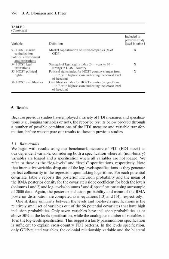
5. Results
Because previous studies have employed a variety of FDI measures and specifica-tions (e.g., logging variables or not), the reported results below proceed througha number of possible combinations of the FDI measure and variable transfor-mation, before we compare our results to those in previous studies.
5.1. Base resultsWe begin with results using our benchmark measure of FDI (FDI stock) asour dependent variable, considering both a specification where all (non-binary)variables are logged and a specification where all variables are not logged. Werefer to these as the “log-levels” and “levels” specifications, respectively. Notethat interactive variables drop out of the log-levels specifications as they generateperfect collinearity in the regression upon taking logarithms. For each potentialcovariate, table 3 reports the posterior inclusion probability and the mean ofthe BMA posterior density for the covariate’s slope coefficient for both the levels(columns 1 and 2) and log-levels (columns 3 and 4) specifications using our sampleof 2000 data. Again, the posterior inclusion probability and mean of the BMAposterior distribution are computed as in equations (13) and (14), respectively.
One striking similarity between the levels and log-levels specifications is therelatively small set of variables out of the 56 potential covariates that have highinclusion probabilities. Only seven variables have inclusion probabilities at orabove 50% in the levels specification, while the analogous number of variables is16 in the log-levels specification. This suggests a fairly parsimonious specificationis sufficient to explain cross-country FDI patterns. In the levels specification,only GDP-related variables, the colonial relationship variable and the bilateral

Determinants of foreign direct investment 797
TABLE 3Level and log-level regressions to explain FDI stocks in 2000
Levels Log-levels
Variable Inclusion Posterior Inclusion Posteriorprobability mean probability mean
1. PARENT real GDP 100 6,322.22 100 1.402. HOST real GDP 100 6,606.47 100 1.743. Distance 39 −0.15 100 −0.944. PARENT real GDP per capita 9 0.05 100 2.315. HOST real GDP per capita 1 0.00 2 0.016. Sum of HOST and PARENT real GDP 0 0.00 0 0.007. Similarity of HOST and PARENT real
GDP86 21,097.71 2 0.00
8. Squared GDP difference 100 −326.09 1 0.009. Squared GDP per capita difference 8 0.00 1 0.0010. HOST urban concentration 0 0.08 52 0.6311. PARENT urban concentration 0 0.00 1 0.0012. Contiguous border 3 158.15 1 0.0013. HOST remoteness 0 0.00 100 2.2914. PARENT remoteness 2 −0.01 30 0.2715. Time zone differences 4 −15.68 5 0.0116. HOST education level 0 −0.03 1 0.0017. HOST skill level 39 6,090.09 97 1.9418. PARENT education level 0 0.67 1 0.0019. PARENT skill level 1 83.09 1 0.0020. Squared education difference 0 −0.04 7 −0.0121. Squared skill difference 1 0.00 89 1.1122. Interaction of GDP differences with
education differences100 −3.53 NA NA
23. Interaction of GDP differences with skilldifferences
0 −5.02 NA NA
24. HOST capital per worker 4 −0.01 1 0.0025. PARENT capital per worker 8 −0.02 36 0.2526. Squared difference in capital per worker 1 0.01 4 0.0027. HOST land area 7 0.00 3 0.0028. PARENT land area 1 0.00 1 0.0029. HOST population density 0 0.52 3 0.0130. HOST is oil country 2 −67.25 92 −0.9231. Common official language 39 2,613.06 92 1.0832. Common language overlap 1 13.52 1 0.0033. Colonial relationship 81 8,071.84 87 1.1434. HOST trade openness 6 1.63 95 0.7935. PARENT trade openness 0 0.05 1 0.0036. Interaction of education differences with
HOST trade openness0 0.00 NA NA
37. Interaction of skill differences with HOSTtrade openness
1 1.42 NA NA
38. Regional trade agreement 0 8.80 100 1.4739. Customs union 1 22.61 97 1.1540. Service sector agreement 49 2,887.97 4 0.0341. HOST time to enforce contract 0 0.01 1 0.0042. HOST time to register property 3 −0.61 26 0.0543. HOST time to start business 6 −2.27 3 −0.0144. HOST time to resolve insolvency 0 −0.16 1 0.0045. HOST corporate tax 0 0.07 67 −0.56
(Continued)

798 B. A. Blonigen and J. Piger
TABLE 3(Continued)
Levels Log-levels
Variable Inclusion Posterior Inclusion Posteriorprobability mean probability mean
46. HOST is tax haven 0 10.81 4 0.1047. Bilateral investment treaty 50 −1,838.23 1 0.0048. Double taxation treaty 0 −3.21 23 0.1049. HOST telephones 2 −0.72 1 0.0050. HOST Internet users 2 0.80 1 0.0051. HOST computers 6 5.28 2 0.0052. HOST domestic credit 3 0.63 1 0.0053. HOST market capitalization 4 0.72 7 0.0254. HOST legal institutions 1 5.72 85 −0.6855. HOST political rights 0 −1.09 5 −0.0256. HOST civil liberties 1 −9.07 1 0.00Sample size 1,066 1,066
NOTES: “Inclusion probability” refers to the posterior probability that the associated variable is inthe true FDI determinants model. “NA” denotes “not applicable” when the variable is not includedbecause it is perfectly collinear with other variables once logged.
investment treaty variable have high inclusion probabilities for explaining FDIstock.
Our preferred specification is the log-levels specification because of the sub-stantial skewness in the dependent variable. In that specification, the evidencesuggests that standard gravity variables with a few friction variables comprisethe bulk of the variables with explanatory power for cross-country FDI patterns.The key gravity variables—real GDP for the host and parent countries, distance,common language and colonial relationships—all have inclusion probabilitiesabove 85% in the log-levels specification. In addition, the trade openness vari-ables indicating the presence of a custom union, the presence of a regional tradeagreement and host-country country openness, all have inclusion values above90%. There is also evidence that endowment differences across the host andparent country may matter, as predicted by some models of FDI, such as theknowledge-capital model of CMM (2001). The host-country skill level and thesquared skill difference between the host and parent country have high inclusionprobabilities, though all other endowment variables (including those capturingcapital and land differences) have very low inclusion probabilities.14 In general,other broad categories of variables receive little statistical support, particularlythose related to business costs, infrastructure and institutions in the host country.The exception is some support for legal institutions (85%) and the corporate taxlevel (67%) in the host country. On the other hand, there are a few variables not
14 The exception is an indicator for whether the host country is an oil-producing country.However, as will be discussed in section 5.3, oil production in the host country is associated withreduced FDI rather than increased FDI.

Determinants of foreign direct investment 799
TABLE 4Inclusion probabilities above 50% using alternative measures of FDI (logged 2000 data)
Variable FDI stock Affiliate sales Cross-border M&A
PARENT real GDP 100 100 100HOST real GDP 100 100 100Distance 100 100 100PARENT real GDP per capita 100 99 100HOST remoteness 100 100 100Regional trade agreement 100 4 100Customs union 97 1 100HOST skill level 97 1 100HOST trade openness 95 3 2Common official language 92 1 100HOST is oil country 92 1 94Squared skill difference 89 2 10Colonial relationship 87 1 97HOST legal institutions 85 22 1HOST corporate tax 67 95 3HOST urban concentration 52 0 1PARENT remoteness 30 0 100Squared GDP per capita difference 1 82 2PARENT urban concentration 1 0 98PARENT skill level 1 1 100HOST time to resolve insolvency 1 2 91
Sample size 1,066 395 1,066
NOTES: The table displays all variables that have at least a 50% inclusion probability in one of thelisted specifications. Instances where the inclusion probability is 50% or higher are in bold.
typically included in empirical FDI studies that have very high inclusion proba-bility in our log-levels specification. These are real GDP per capita in the parentcountry (100%), remoteness of the host country (100%) and, to a lesser extent,urban concentration of the host country (52%).
Our results to this point use FDI stock as our measure of cross-countryFDI activity. Table 4 next compares results when we use two other measures ofFDI that have been used by prior studies—affiliate sales and cross-border M&Aactivity. The table displays all variables that receive at least 50% in one of ourthree specifications (FDI stock, affiliate sales or M&A). For ease in reading thetable, we bold the instances where the inclusion probability is 50% or higher.For comparison sake, we report only the results for the log-levels specification,and, for the M&A sample, we use only observations for the 1,066 country pairsfor which we observe the FDI stock variable. (We have many more country-pairobservations for the M&A sample that we will analyze and discuss below.) We useall observations available for affiliate sales, but this provides just 395 observations.
Despite these data issues, many of the patterns found in the FDI stock specifi-cation are also found when using these other FDI measures. First, the traditionalgravity variables (real GDP of both countries and distance) all have inclusionprobabilities of 100% across all three specifications. Parent-country real GDP per

800 B. A. Blonigen and J. Piger
capita also has at least a 99% inclusion probability across all three, suggestingthat the wealth of the source country is a key determinant of FDI. Interest-ingly, host country real GDP per capita does not have similarly high inclusionprobabilities. There is a similar asymmetry in that host country remotenessgenerally garners high inclusion probabilities across all the measures of FDIactivity, whereas parent country remoteness does not. It has a high inclusionprobability only in the cross-border M&A specification. These asymmetric re-sults are an example of empirical patterns our analysis finds that have not beenexamined by prior theory or empirical studies of FDI to our knowledge.
In general, the M&A and FDI stock samples share many variables with highinclusion probabilities beyond the ones we have mentioned, including commonofficial language, colonial relationship, regional trade agreement, customs union,host oil country and host skill level. One interesting difference between the M&Aand FDI stock results are that while legal institutions and corporate taxes in thehost country have modestly high inclusion probabilities for FDI stock, theyhave very low ones in the M&A sample. Instead, days to resolve insolvencies inthe host country is the only host country business cost variable to have a highinclusion variable in the M&A sample. One final notable difference is that parent-country remoteness and urban concentration have high inclusion probabilities inthe M&A sample, but not in the other samples.
The FDI stock and affiliate sales specifications find less commonality in thevariables that have high inclusion probabilities. We have also produced results forthe FDI stock and affiliate sales specifications on a common, overlapping sampleof 253 observations and found much more similarity in results that mirror thosefor affiliate sales in table 4. This suggests that the differences across the affiliatesales and FDI stock specifications in table 4 are due primarily to the relativelysmall sample available for the affiliate sales measure. Overall, the general patternsnoted in earlier specifications reported above continue to hold—gravity finds verystrong support, while cultural distance and endowment variables find support aswell. In contrast, there continues to be much less support for variables capturinghost country business costs, infrastructure or institutions.
As mentioned, the data on FDI stock and affiliate sales is limited primarilyto OECD country pairs, though there is some information on FDI from OECDinto less-developed countries, but not on FDI patterns between less-developedcountries. On the one hand, this selection may not be a significant issue be-cause the vast majority of FDI in the world economy is between the developedeconomies, which are well represented in our sample. On the other hand, it isuseful to know how FDI determinants may differ when a more representativesample of countries is examined. Our M&A data source has the ability to addressthis as it is a census of worldwide M&A activity.
Table 5 lists all variables with inclusion variables above 50% for three specifi-cations using logged data for the year 2000. The first two columns of inclusionprobabilities are for comparison purposes and are for the FDI stock specifica-tion and the M&A specification when limited to the same observations as the

Determinants of foreign direct investment 801
TABLE 5Inclusion probabilities above 50% for OECD and worldwide samples (logged 2000 data)
OECD sample Worldwide sample
Variable FDI stock Cross-border M&A Cross-border M&A
HOST real GDP 100 100 100PARENT real GDP 100 100 100Distance 100 100 100PARENT real GDP per capita 100 100 100HOST remoteness 100 100 100Regional trade agreement 100 100 100Customs union 97 100 100HOST skill level 97 100 71HOST country trade openness 95 2 2Common official language 92 100 99HOST is oil country 92 94 92Squared skill difference 89 10 3Colonial relationship 87 97 100HOST legal institutions 85 1 1HOST corporate tax 67 3 99HOST urban concentration 52 1 1PARENT remoteness 30 100 100Double taxation treaty 23 2 100Squared education difference 7 38 97Service sector agreement 4 1 97Similarity of HOST and PARENT real GDP 2 1 54PARENT education level 1 1 85PARENT urban concentration 1 98 100PARENT skill level 1 100 76Bilateral investment treaty 1 14 100HOST education level 1 3 100HOST years to resolve insolvency 1 91 98Contiguous border 1 1 95
Observations 1,066 1,066 3,429
NOTES: The table displays all variables that have at least a 50% inclusion probability in one of thelisted specifications. Instances where the inclusion probability is 50% or higher are in bold.
FDI stock sample. The third column is the M&A specification when we use allobservations for which we have available data (we call this the “worldwide” sam-ple), as opposed to the restricted sample (we call this the “OECD” sample). Thismore than triples the sample size over the other two listed specifications to 3,429observations, adding many more observations involving non-OECD countries.15
The results from the worldwide M&A sample show a lot of commonalities withthe previous results. Gravity variables, cultural distance and relative skilled labourvariables all show very high inclusion probabilities. In fact, all of the variablesthat have high inclusion probabilities in the OECD M&A sample specification(column 2) also have high inclusion probabilities in the worldwide M&A sample
15 In the “OECD” sample, all country-pair observations involve at least one OECD country, and40% of the country-pair observations are between OECD countries. In the “worldwide” sample,32% of the country-pair observations do not involve at least one OECD country, and only 18%of the country-pair observations are between OECD countries.

802 B. A. Blonigen and J. Piger
specification. However, the worldwide M&A sample also shows high inclusionprobabilities for a number of additional variables. These include a few moreendowment variables (education levels in both the host and parent country as wellas the squared difference in education levels between the two countries), as onemight expect when one includes many more observations between relatively poornon-OECD countries and OECD countries. It also includes variables connectedwith bilateral treaties (bilateral investment treaty, double taxation treaty andservice sector agreements) as well as the presence of a contiguous border. Thissuggests that these bilateral treaties may be much more important for spurringFDI into non-OECD countries than into OECD ones.
5.2. Implications for prior studiesWith our BMA results in hand, we now turn to address the fundamental questionof how our BMA results compare to those of previous studies. Virtually all of theprior studies include gravity-related variables, and, thus, our results confirm theinclusion of such variables. Common official language also finds robust supportin our analysis and is included in five of the prior eight studies in table 1. Beyondthis small set of variables, however, prior studies vary significantly in what theyinclude, and what they include does not necessarily match very well with thevariables our analysis finds to have high inclusion probabilities. For example, ouranalysis finds that parent country wealth (real per capita GDP) has strong androbust support, yet only one study (Head and Ries 2008) of the eight studiesin table 1 includes this variable. In contrast, four of the studies in table 1 in-clude host country wealth, yet we find this variable does not have strong supportfor inclusion. The reason for this asymmetry in wealth effects on FDI is alsosomething that past theoretical papers, to our knowledge, do not address. Onlyfour of the prior eight studies include variables related to relative skilled-labourendowment levels or differences, whereas our analysis finds that such variablesshould be included. There is little evidence that other relative endowments matterbesides the presence of oil in the host country. Colonial relationships, host coun-try remoteness, trade agreements and customs unions are additional variablesthat find strong support in our analysis but are rarely included in prior studies.On the other hand, a number of the prior studies include variables connectedto host country business costs, infrastructure and institutions, but these do notfind robust support in our analysis. Finally, the studies in table 1 whose mainfocus is on a particular hypothesized relationship between a potential covariateand FDI generally do not fare very well in terms of the inclusion probabilitieswe estimate for the same covariate. This includes Wei (2000), whose focus is oncorruption; Stein and Daude (2007), whose focus is on time zone differences; anddi Giovanni (2005), whose partial focus is on financial market institutions.
5.3. Slope coefficient magnitudesTo this point, we have focused only on inclusion probabilities. In table 6, we reportestimates of the slope coefficient of the variables listed in table 5. In particular,

Determinants of foreign direct investment 803
TABLE 6Posterior mean and variance of slope coefficients for OECD and worldwide samples (logged 2000data)
OECD sample Worldwide sample
Variable FDI stock Cross-border M&A Cross-border M&A
HOST real GDP 1.74 (0.02) 0.97 (0.00) 0.61 (0.00)PARENT real GDP 1.40 (0.00) 1.02 (0.00) 0.79 (0.00)Distance −0.94 (0.02) −0.63 (0.01) −0.44 (0.00)PARENT real GDP per
capita2.31 (0.14) 1.29 (0.01) 0.61 (0.01)
HOST remoteness 2.29 (0.24) 1.24 (0.05) 0.64 (0.01)Regional trade agreement 1.47 (0.09) 1.37 (0.04) 1.19 (0.02)Customs union 1.15 (0.11) 1.23 (0.04) 0.92 (0.04)HOST skill level 1.94 (0.36) 1.40 (0.08) 0.26 (0.04)HOST country trade
openness0.79 (0.07) 0.00 (0.00) 0.00 (0.00)
Common official language 1.08 (0.20) 1.08 (0.04) 0.45 (0.01)HOST is oil country −0.92 (0.13) −0.56 (0.04) −0.29 (0.01)Squared skill difference 1.11 (0.25) 0.05 (0.03) 0.01 (0.00)Colonial relationship 1.14 (0.31) 0.93 (0.08) 1.22 (0.02)HOST legal institutions −0.68 (0.12) 0.00 (0.00) 0.00 (0.00)HOST corporate tax −0.56 (0.19) −0.01 (0.00) −0.32 (0.01)HOST urban concentration 0.63 (0.44) 0.00 (0.00) 0.00 (0.00)PARENT remoteness 0.27 (0.21) 1.17 (0.05) 0.59 (0.01)Double taxation treaty 0.10 (0.04) 0.00 (0.00) 0.42 (0.00)Squared education
difference−0.01 (0.00) −0.03 (0.00) −0.06 (0.00)
Service sector agreement 0.03 (0.03) 0.00 (0.00) 0.68 (0.05)Similarity of HOST and
PARENT real GDP0.00 (0.00) 0.00 (0.00) 0.13 (0.02)
PARENT education level 0.00 (0.00) 0.00 (0.00) 0.34 (0.03)PARENT urban
concentration0.00 (0.00) −0.76 (0.05) −0.50 (0.00)
PARENT skill level 0.00 (0.00) 1.19 (0.06) 0.32 (0.05)Bilateral investment treaty 0.00 (0.00) −0.04 (0.01) −0.36 (0.00)HOST education level 0.00 (0.00) 0.01 (0.00) 0.69 (0.02)HOST years to resolve
insolvency0.00 (0.00) 0.25 (0.01) 0.15 (0.00)
Contiguous border 0.00 (0.00) 0.00 (0.00) 0.21 (0.01)
Observations 1,066 1,066 3,429
NOTES: The table displays the posterior mean and variance (in parentheses) of slope coefficientfor all variables that have 50% or higher inclusion probability for at least one of the listedspecifications. Coefficients where the associated inclusion probability is 50% or higher are inbold.
for the variables and specifications in table 5, we report the mean and variance ofthe BMA posterior density for the slope coefficient on each variable, calculatedas inequations (14) and (15). With few exceptions, the coefficient signs are asone would expect and consistent with prior studies. This includes the gravityvariables, cultural distance variables and bilateral trade openness variables. Formany of the coefficients, the magnitude of the effect is smaller in the worldwideM&A sample than for the OECD sample, which suggests that FDI responds

804 B. A. Blonigen and J. Piger
much less to economic forces for host countries that are less developed. A few ofthe coefficients have unexpected signs. One of the more intriguing results is thatwhile the bilateral distance between country pairs lowers FDI (as expected), theremoteness of both the parent and host countries (that is, how far they are fromthe entire world’s markets, not just the other country in the country pair) haspositive coefficients. This distinction has not been made before to our knowledgebut certainly deserves future investigation. Another surprising result is that thepresence of oil in the host country is associated with lower FDI, as is the strengthof host country legal institutions.
The posterior mean and variance of the slope coefficients can also be used toconstruct a “pseudo t-ratio” by dividing the posterior mean by the posterior stan-dard deviation. This statistic is a natural candidate as a measure of the relativeimportance of potential covariates in a linear regression setting and is some-times reported along with BMA inclusion probabilities. In our application, thepseudo t-ratios (not reported) provide very similar conclusions to those reachedfrom the BMA inclusion probabilities regarding the relative importance of thecandidate FDI determinants. As a specific example, for the log-levels specifica-tion using FDI stocks as the dependent variable, the ranking of FDI determi-nants by the two metrics is nearly identical, with the Spearman rank correlationstatistic between the pseudo t-ratio and the BMA inclusion probability equalto 0.98.
5.4. Controlling for country-pair effectsMany prior studies of FDI determinants include country or country-pair effects.A simple way to control for such effects is to difference the data by country-pair combinations. Table 7 provides results from log-linear specifications for a1990–2000 differenced sample for our FDI stock, OECD M&A and worldwideM&A samples. First-differencing in this manner eliminates a number of time-invariant variables, as is typical. It unfortunately also eliminates a very largeportion of the observations, due to many more missing values for variables in1990. This may be why the FDI stock and OECD M&A samples have onlyone variable between them that comes in with an inclusion probability over50%, though a possible alternative explanation is that bilateral FDI patterns arelargely driven by slow-moving or time-invariant factors that are then differencedout of these regressions. However, the worldwide M&A sample still has over1,200 observations and finds 12 variables to have inclusion probabilities over50%. What we find most important is that these high-inclusion probabilitiesin the first-differenced worldwide M&A sample are largely the same ones aswe have found throughout the many varied permutations we have evaluated inthis paper: GDP-related variables, skilled-labour variables and trade agreements.Distance and cultural distance factors do not show up in this table becausefirst-differencing leaves no (or virtually no) variation from which to identify theimpact of these factors.
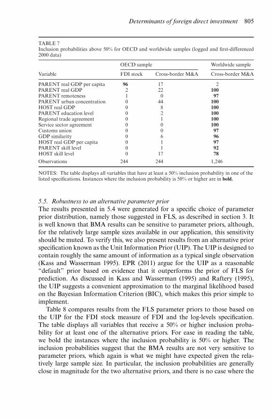
Determinants of foreign direct investment 805
TABLE 7Inclusion probabilities above 50% for OECD and worldwide samples (logged and first-differenced2000 data)
OECD sample Worldwide sample
Variable FDI stock Cross-border M&A Cross-border M&A
PARENT real GDP per capita 96 17 2PARENT real GDP 2 22 100PARENT remoteness 1 0 97PARENT urban concentration 0 44 100HOST real GDP 0 8 100PARENT education level 0 2 100Regional trade agreement 0 1 100Service sector agreement 0 0 100Customs union 0 0 97GDP similarity 0 6 96HOST real GDP per capita 0 1 97PARENT skill level 0 1 92HOST skill level 0 17 78
Observations 244 244 1,246
NOTES: The table displays all variables that have at least a 50% inclusion probability in one of thelisted specifications. Instances where the inclusion probability is 50% or higher are in bold.
5.5. Robustness to an alternative parameter priorThe results presented in 5.4 were generated for a specific choice of parameterprior distribution, namely those suggested in FLS, as described in section 3. Itis well known that BMA results can be sensitive to parameter priors, although,for the relatively large sample sizes available in our application, this sensitivityshould be muted. To verify this, we also present results from an alternative priorspecification known as the Unit Information Prior (UIP). The UIP is designed tocontain roughly the same amount of information as a typical single observation(Kass and Wasserman 1995). EPR (2011) argue for the UIP as a reasonable“default” prior based on evidence that it outperforms the prior of FLS forprediction. As discussed in Kass and Wasserman (1995) and Raftery (1995),the UIP suggests a convenient approximation to the marginal likelihood basedon the Bayesian Information Criterion (BIC), which makes this prior simple toimplement.
Table 8 compares results from the FLS parameter priors to those based onthe UIP for the FDI stock measure of FDI and the log-levels specification.The table displays all variables that receive a 50% or higher inclusion proba-bility for at least one of the alternative priors. For ease in reading the table,we bold the instances where the inclusion probability is 50% or higher. Theinclusion probabilities suggest that the BMA results are not very sensitive toparameter priors, which again is what we might have expected given the rela-tively large sample size. In particular, the inclusion probabilities are generallyclose in magnitude for the two alternative priors, and there is no case where the

806 B. A. Blonigen and J. Piger
TABLE 8Inclusion probabilities above 50% using alternative parameter priors (FDI stock – logged 2000 data)
Variable FLS UIP
PARENT real GDP 100 100HOST real GDP 100 100Distance 100 100PARENT real GDP per capita 100 100HOST remoteness 100 100Regional trade agreement 100 100Customs union 97 97HOST skill level 97 99HOST trade openness 95 97Common official language 92 93HOST is oil country 92 97Squared skill difference 89 97Colonial relationship 87 95HOST legal institutions 85 94HOST corporate tax 67 84HOST urban concentration 52 67PARENT capital per worker 36 50
Observations 1,066 1,066
NOTES: The table displays all variables that have 50% or higher inclusion probability for at leastone of two alternative specifications for parameter priors. Instances where the inclusion probabilityis 50% or higher are in bold. Results are for the FDI stock dataset and log-levels specification. FLSrefers to priors suggested by Fernandez, Ley and Steel (2001a), as described in section 3. UIP refersto the Unit Information Prior of Kass and Wasserman (1995), as described in section 5.
two priors yield radically different conclusions regarding the importance of acovariate.
5.6. Robustness to a nonlinear specificationDue to the computational intensity of the BMA approach, our analysis to thispoint was restricted to linear regression models. However, there are some po-tential issues with a linear specification for the measures of FDI used as thedependent variable. First, there are many country pairs for which the FDI mea-sure is zero. This creates an issue in the log-level regressions, as the logarithm ofthese observations is undefined. In the results presented above, we retained theseobservations in the sample by adding a small constant to each FDI measurebefore taking logarithms. Alternatively, we could have eliminated these obser-vations from the sample. As is discussed in Santos Silva and Tenreyro (2006),each of these solutions might distort inference from that produced by an appro-priate nonlinear model estimated on the levels of the dependent variable. Theseauthors argue for the use of Poisson regression methods to effectively deal withzero observations. Second, our measure of FDI based on M&A activity is a dis-crete count variable, a fact that is ignored when working in the linear regressionframework.

Determinants of foreign direct investment 807
In this section we evaluate the robustness of the conclusions regarding thedeterminants of FDI when a nonlinear model is used to link FDI to potentialcovariates. We focus on M&A counts as the FDI measure, as this data displaysboth of the features discussed above—zero observations and discreteness. We usea negative binomial regression to model the M&A counts. This framework modelsthe level of the M&A counts directly, which eliminates any issues associated withthe need to take logarithms of zero observations. Also, the negative binomialdistribution is a discrete distribution with a natural interpretation for countdata.16
Extending the MC3 algorithm discussed in section 3 for linear regression mod-els to conduct BMA for negative binomial regressions is conceptually straightfor-ward. Specifically, the only change is that the marginal likelihood in (3) is replacedby the marginal likelihood for the negative binomial model. Unfortunately, unlikethe case of the linear regression model with natural conjugate priors, the marginallikelihood for the negative binomial model is not available analytically and needsto be approximated. One approach would be to compute a simulation-consistentestimate of the marginal likelihood using Markov chain Monte Carlo techniques.However, when incorporated inside of the large number of simulations necessaryfor the MC3 algorithm, this would be very computationally demanding. Instead,we use an asymptotic approximation to the marginal likelihood based on the BIC.This requires only the maximum likelihood estimates of the negative binomialregression and can be computed relatively quickly.17
Table 9 shows the posterior inclusion probabilities computed for the log-levellinear regression model, along with those based on the negative binomial model,when we use the sample of cross-border M&A counts across OECD countries,i.e., the sample identical to the one used in the last column of table 4. We use thesample of OECD countries, rather than the larger worldwide sample, to reducethe computational time needed to calculate the SIC for the negative binomialspecification. Results across the linear and negative binomial models are verysimilar, suggesting model misspecification bias from running linear models in thissetting is small. Out of 52 potential covariates, there are only four instances wherethe inclusion probability of a covariate is very high in one specification but closeto zero in the other. In particular, urban concentration of the parent countryand host country oil production have very high inclusion probabilities in thelinear specification but inclusion probabilities near zero in the negative binomial
16 A common starting point for modelling count data is the Poisson regression model. However,our sample of M&A count data has sample variance far greater than sample mean, suggesting amodel that incorporates this overdispersion is better suited for M&A counts. The negativebinomial regression model, which arises from a natural extension of the Poisson regression, is apopular choice for overdispersed count data in the applied literature. Indeed, we experiencedsubstantial convergence issues when estimating a simple Poisson specification, which furtherindicated that it is important to model overdispersion in these data.
17 The BIC approximation to the marginal likelihood is a common choice in applied work. See, forexample, Brock, Durlauf and West (2003) and Doppelhofer, Miller and Sala-i-Martin (2004).For additional discussion of the BIC-based approach to model averaging, see Raftery (1995).

808 B. A. Blonigen and J. Piger
TABLE 9Inclusion probabilities for linear and negative binomial specifications (cross-border M&A for OECDsample – logged 2000 data)
Variable Linear model Negative binomial
HOST real GDP 100 100PARENT real GDP 100 100Distance 100 100PARENT real GDP per capita 100 100HOST remoteness 100 100Regional trade agreement 100 100Customs union 100 100HOST skill level 100 100Common official language 100 100PARENT remoteness 100 100PARENT skill level 100 95PARENT urban concentration 98 2Colonial relationship 97 100HOST is oil country 94 0HOST years to resolve insolvency 91 100Squared education difference 38 95HOST political rights 12 100HOST country trade openness 2 64Similarity of HOST and PARENT real GDP 1 98HOST legal institutions 1 53
Observations 1,066 1,066
NOTES: The table displays the inclusion probability for every potential covariate listed intable 2, with the exception of the interaction terms, which become perfectly collinear when variablesare logged.
specification, while GDP similarity and host country political rights are estimatedto have high inclusion probabilities in the negative binomial specification butinclusion probabilities near zero in the linear model. Three other variables, thesquared education difference, host country trade openness and host country legalinstitutions, receive more support in the negative binomial specification, withinclusion probabilities roughly 50 percentage points above those for the linearmodel. Outside of these seven exceptions, which is less than 15% of the covariateswe consider, the average absolute difference in inclusion probabilities across thelinear and negative binomial models is just 2.6 percentage points. Also, it isnotable that of the five variables for which the negative binomial model providesmore support than the linear model, four have high inclusion probabilities for thelinear model applied to the FDI stock or worldwide sample M&A count data.Thus, the negative binomial specification is not revealing a substantial number ofadditional relevant covariates beyond those identified elsewhere in our analysis.
5.7. BMA on trade flowsA related BMA analysis we can perform using our covariates is an examina-tion of the determinants of trade flows. This is an interesting litmus test for theBMA procedure, as we would be concerned, for example, if standard gravityvariables did not have high inclusion probabilities for trade flows using our BMA

Determinants of foreign direct investment 809
TABLE 10Inclusion probabilities above 50% for explaining FDI vs. bilateral trade (worldwide sample – logged2000 data)
Variable Cross-border M&A Bilateral trade
PARENT real GDP 100 100HOST real GDP 100 100Distance 100 100PARENT real GDP per capita 100 100HOST remoteness 100 100PARENT remoteness 100 100Regional trade agreement 100 100Customs union 100 100Colonial relationship 100 94HOST education level 100 13Double taxation treaty 100 100Bilateral investment treaty 100 100Parent urban concentration 100 1Common official language 99 96HOST corporate tax 99 20HOST time to resolve insolvency 98 6Squared education difference 97 1Service sector agreement 97 2Contiguous border 95 19HOST is oil country 92 62PARENT education level 85 100PARENT skill level 76 1HOST skill level 71 0Similarity of HOST and PARENT real GDP 54 100PARENT trade openness 4 98Squared skill difference 3 100HOST trade openness 2 51HOST land area 2 95HOST legal institutions 1 100HOST urban concentration 1 60HOST Internet users 1 100HOST domestic credit 1 70HOST time to start business 1 99
Observations 3,429 3,429
methods. The analysis also provides a comparison of the determinants of FDI andtrade flows within the same framework. We gather data on bilateral trade flowsfrom the dataset connected with Rose and Spiegel (2011) and made available on-line by Andrew Rose at faculty.haas.berkeley.edu/arose/RecRes.htm#Software.Specifically, the data are CIF imports measured in US$, taken from Interna-tional Financial Statistics’ Direction of Trade CD-ROM, deflated by U.S. CPIfor All Urban Consumers (CPI-U), all items, 1982 to 1984 = 100. For compari-son purposes, we sample the year 2000 for the same observations we use for ourcross-border M&A results, which yielded the largest sample size out of all theFDI measures.
Table 10 provides inclusion probabilities for our BMA analysis of trade flows,as well as repeats the cross-border M&A inclusion probabilities for comparison
810 B. A. Blonigen and J. Piger
purposes. The table displays all variables that receive a 50% or higher inclusionprobability for explaining at least one of either trade flows or M&A counts.Reassuringly, our BMA analysis of trade flows yields results that are quite in linewith accepted practice on how to specify trade flows. The gravity variables andtypical frictions (including trade and FDI agreements) show very strong support.This also means that our analysis suggests very similar determinants for trade andcross-border M&A, though there is much less support generally for endowmentterms with trade than for cross-border M&A. The biggest differences between thetwo come in which business cost, infrastructure and other host-country attributesmatter for trade versus cross-border M&A. For example, the number of Internetusers, legal institutions and domestic credit have high inclusion probabilities fortrade but not for cross-border M&A.
This is not the first BMA analysis of trade flows. Eicher, Henn andPapageorgiou (2012) use BMA methods to examine the impact of preferentialtrade agreements on trade flows. They estimate very similar inclusion probabili-ties for the common overlap of variables between their study and ours, includingstrong support for GDP terms, geographic features (such as distance) and cul-tural distance terms.
6. Conclusion
The prior literature examining the determinants of FDI comprises a limitednumber of studies that typically propose fairly parsimonious specifications, butquite varied in their specifications and FDI measurement. This suggests signifi-cant uncertainty in the true model of bilateral cross-country FDI patterns. Ourapproach is to provide some needed systematic investigation of the determinantsof FDI by using Bayesian Model Averaging. Our analysis does not support theinclusion of many variables found in prior FDI studies and suggests that the sta-tistical importance of the main focus variables in many prior studies is not robustto considering a much wider set of covariates. The results also suggest a fairlyparsimonious FDI specification comprised of mainly gravity variables, culturaldistance factors, parent-country per capita GDP, relative labour endowmentsand trade agreements.
Of note, our results reflect much less support for government policies toencourage FDI, as there is little robust evidence in our analysis that policyvariables controlled by the host country (such as multilateral trade costs, businesscosts, infrastructure or political institutions) have an effect on FDI. Exceptionsinclude policies that are often negotiated bilateral agreements, including tradeagreements, bilateral investment treaties, customs unions and service agreementsin the case of M&A. However, we caution that exogeneity of these variables maybe more in doubt than many of the other covariates we consider.

Determinants of foreign direct investment 811
References
Baltagi, B.H., P. Egger and M. Pfaffermayr (2007) “Estimating models of complex FDI:Are there third-country effects,” Journal of Econometrics 140, 260–81
Bergstrand, J.H., and P. Egger (2007) “A knowledge-and-physical-capital model ofinternational trade flows, foreign direct investment, and multinational enterprises,”Journal of International Economics 73, 278–308
Blonigen, B.A., R. B. Davies, G. R. Waddell and H. Naughton (2007) “FDI in space:Spatial autoregressive relationships in foreign direct investment,” European EconomicReview 51, 1303–25
Braconier, H., P.-J. Norback and D. Urban (2005) “Reconciling the evidence on theknowledge-capital model,” Review of International Economics 13, 770–86
Brock, W.A., S. N. Durlauf and K. D. West (2003) “Policy evaluation in uncertaineconomic environments,” Brookings Papers on Economic Activity 1, 235–301
Carr, D., J. R. Markusen and K. E. Maskus (2001) “Estimating the knowledge–capitalmodel of the multinational enterprise,” American Economic Review 91, 693–708
Chakrabarti, A. (2001) “The determinants of foreign direct investment: Sensitivityanalyses of cross-country regressions,” Kyklos 54, 89–114
di Giovanni, J. (2005) “What drives capital flows? The case of cross-border M&Aactivity and financial deepening,” Journal of International Economics 65, 127–49
Doppelhofer, G., R. I. Miller and X. Sala-i-Martin (2004) “Determinants of long-termgrowth: A Bayesian averaging of classical estimates (BACE) approach,” AmericanEconomic Review 94, 813–35
Draper, D. (1995) “Assessment and propagation of model uncertainty (withdiscussion),” Journal of the Royal Statistical Society, Series B 57, 45–97
Eaton, J., and A. Tamura (1994) “Bilateralism and regionalism in Japanese and U.S.trade and direct foreign investment patterns,” Journal of the Japanese andInternational Economies 8, 478–510
Eicher, T.S., L. Helfman and A. Lenkoski (2010) “Robust FDI determinants,” Journal ofMacroeconomics, forthcoming
Eicher, T.S., C. Henn and C. Papageorgiou. (2012) “Trade creation and diversionrevisited: Accounting for model uncertainty and natural trading partner effects,”Journal of Applied Econometrics 27, 296–321
Eicher, T.S., C. Papageorgiou and A. E. Raftery (2011) “Default priors and predictiveperformance in Bayesian model averaging, with application to growth determinants,”Journal of Applied Econometrics 26, 30–55
Fernandez, C., E. Ley and M. F. J. Steel (2001a) “Benchmark priors for Bayesian modelaveraging,” Journal of Econometrics 100, 381–427
——— (2001b) “Model uncertainty in cross country growth regressions,” Journal ofApplied Econometrics 16, 563–76
Head, K., and J. Ries (2008) “FDI as an outcome of the market for corporate control:Theory and evidence,” Journal of International Economics 74, 2–20
Hodges, J.S. (1987) “Uncertainty, policy analysis, and statistics,” Statistical Science 2,259–91
Hoeting, J.A., D. Madigan, A. E. Raftery and C. T. Volinsky (1999) “Bayesian modelaveraging: A tutorial (with discussion),” Statistical Science 14, 382–401
Jordan, A., and A. Lenkoski (2012), “Tobit Bayesian model averaging and thedeterminants of foreign direct investment,” mimeo
Kass, R.E., and A. E. Raftery (1995) “Bayes factors,” Journal of the American StatisticalAssociation 90, 773–95

812 B. A. Blonigen and J. Piger
Kass, R.E., and L. Wasserman (1995) “A reference Bayesian test for nested hypothesesand its relationship to the Schwarz criterion,” Journal of the American StatisticalAssociation 90, 928–34
Koop, G. (2003) Bayesian Econometrics. Hoboken, NJ: J. WileyLeamer, E.E. (1978) Specification Searches: Ad Hoc Inference with Nonexperimental
Data. New York, NY: WileyLey, E., and M. F. J. Steel (2009) “On the effect of prior assumptions in Bayesian model
averaging with applications to growth regression,” Journal of Applied Econometrics24, 651–74
Madigan, D., and J. York (1995) “Bayesian Graphical Models for Discrete Data,”International Statistical Review 63, 215–32
Magnus, J.R., O. Powell and P. Prufer (2010) “A comparison of two model averagingtechniques with an application to growth empirics,” Journal of Econometrics 154,139–53
Moulton, B.R. (1991) “A Bayesian approach to regression selection and estimation withapplication to a price index for radio services,” Journal of Econometrics 49, 169–93
Raftery, A.E. (1995) “Bayesian model selection for social research,” SociologicalMethodology 25, 111–63
——— (1996) “Approximate Bayes factors and accounting for model uncertainty ingeneralised linear models,” Biometrika 83, 251–66
Raftery, A.E., D. Madigan and J. A. Hoeting (1997) “Bayesian model averaging forlinear regression models,” Journal of the American Statistical Association 92, 179–91
Rose, A.K., and M. M. Spiegel. (2011) “The Olympic effect,” Economic Journal 121,652–77
Rossi, S., and P. F. Volpin (2004) “Cross-country determinants of mergers andacquisitions,” Journal of International Economics 74, 277–304
Santos Silva, J.M.C., and S. Tenreyro (2006) “The log of gravity,” Review of Economicsand Statistics 88, 641–58
Stein, E., and C. Daude (2007) “Longitude matters: Time zones and the location offoreign direct investment,” Journal of International Economics 71, 96–122
Wei, S-J. (2000) “How taxing is corruption on international business,” Review ofEconomics and Statistics 82, 1–11
Zellner, A. (1986) “On assessing prior distributions and Bayesian regression analysiswith g-prior distributions,” in Bayesian Inference and Decision Techniques: Essays inHonour of Bruno de Finetti., eds. P.K. Goel and A. Zellner. Amsterdam: NorthHolland