determinants of demand for money and the velocity …

JDE (Journal of Developing Economies) Vol. 3 No. 2 (2018): 65-79

JDE (Journal of Developing Economies)https://e-journal.unair.ac.id/JDE/index

DETERMINANTS OF DEMAND FOR MONEY AND THE VELOCITY OF MONEY IN INDONESIA

Alvin Sugeng Prasetyo*¹

¹Universitas Trunojoyo, Indonesia

ABSTRACT

The demand for money is one of many monetary economics topics that is popular in every country. This study aims to test and analyze some influ-ential factors of the demand for money and the velocity of money in Indo-nesia. The data source of this study takes from the International Financial Statistics. The method used is ARDL with a period of 2000Q1- 2017Q4. The result of the analysis shows that all the variables are stationary on the I (0), a Bound test shows there are cointegration and the selected model that is ARDL (4, 2, 0, 0, 0). The study concludes that the economic growth and the growth rate of the rupiah/USD give a significant effect toward the growth of M2 in the long term and short term, and the velocity of money in Indonesia has an increased trend.

Keywords: M2, ARDL, economic growth, the growth rate of the rupiah/USD

JEL Classification: O49,

To cite this document: Prasetyo, A.S.,(2018). Determinants of Demand For Money and The Velocity of Money In Indonesia. JDE (Journal of

Developing Economies), 3(2) , 65-79.

Introduction

The demand for money is a certain amount of money that is held by private sectors. The private sectors hold the money because of two important functions that are money as a medium of exchange and a store of value. The demand for money for a medium of ex-change means that money serves to facilitate trade transactions in goods and services, while the de-mand for money for a store of value means money forms wealth, due to the two functions of the money, so that money demand is an important part of the topic of monetary economics (Bitrus, 20110). Hence, it makes the topic of money demand is often empirically tested by aca-demics.

Demand for money is a popular topic among academics because it is one of the vari-ables that is very concerned about compiling the monetary policy framework (Sichei and Ka-mau, 2012). Monetary policy makers give a high attention toward the demand for money be-cause its stability and good management makes monetary policy becomes more effective in JDE (Journal of Developing Economies) p-ISSN: 2541-1012; e-ISSN: 2528-2018DOI:10.20473/jde.v3i2.10464Open access under a Creative Commons Attribution 4.0 International

(CC-BY)

ARTICLE INFOReceived: November 11st, 2018 Revised: November 29th, 2018Accepted: December 11st, 2018Online: December 25th, 2018

*Correspondence: Alvin Sugeng PrasetyoE-mail: [email protected]

https://creativecommons.org/licenses/by/4.0/

mailto:[email protected]

mailto:[email protected]

66

Prasetyo, A. S. Determinants of Demand For Money and The Velocity of Money In Indonesia

which it is able to give a positive impact to the economy itself.

The empirical determination of money demand can be implemented by using a sample of Indonesian research. Indonesia is one of the developing countries that use money as a tool for consumption, investment and saving activities. Demand for money in Indonesia has many types in which it is divided into 3 types of money, namely M0, M1, and M2. M0 is the monetary base, or base money that is pulished and controlled by the Bank of Indonesia. The definition of M0 is Bank Indonesia’s liabilities by the commercial banks, rural banks, and the private sector. Furthermore, M1 is a certain amount of cur-rency owned by the domestic private sector and current accounts in rupiah. M1 is a nar-row money that generally considers larger than M0. The definition of M2 is a certain amount of narrow money and quasi-money. Quasi-money consists of time deposits (denomi-nated in rupiah and foreign currency), savings deposits (denominat-ed in rupiah and foreign currency), and deposits demand (denominated in foreign currency)(Suseno and Solikin, 2002, pp. 21–26). The amount of narrow money and quasi-money also calls as the broad money.

Figure 1 for the 2010-2012 and 2015-2016 periods shows that M1 growth is above M2 growth. The condition means that there is an increased activity in the real sector. The emerg-ing of increased activity in Indonesian’s real sector is followed by the indicators of household consumption, government consumption, and exports. If these three indicators increase, the real sector will also increase. Furthermore, the increase in M2 is influenced by an increase in in-flows of foreign funds which is mostly placed as quasi-money in banks (BI, 2010).

Figure 1 shows conditions that are different from the previous period. M2 growth was above M1 growth during the 2012-2014 periods, so that real sector activity experienced a slowdown, and people preferred to save in commercial banks. M2 growth that is above M1 growth also indicates that Indonesian people’s activities with broad money transactions have increased as well as followed by a declining M2 growth. It is because Net Domestic Assets (NDA) and M1 have decreased (BI, 2013). The slowdown in M1 growth is caused by a slow-down in currency and demand deposits growth.

Figure 1: Narrowand Broad Money in Indonesia 2010-2016 (in percent)Source: Bank Indonesia A velocity of money also relates to the demand for money that needs to be analyzed. The velocity of money is given the symbol V. Velocity of money shows the average number

67


of its rotation times in one year from one unit of currency used to buy goods and services in the economy (Mishkin, 2004, p. 517). The velocity of money can be calculated by the ratio be-tween nominal GDP and the money supply. If a country’s nominal GDP grows faster than the growth of a money supply, then the velocity of money increases (Rami, 2010).

The effect of economic growth on the demand for money is based on the transaction and preventive motives. The demand for money of transactions and preventive motives is de-termined by the level of income. High-income people will do more transactions than low-in-come people will. Thus, the higher level of economic growth in a country will also influence the higher level of a person’s income and a demand for money for doing transactions and preventive motives.

The exchange rate becomes an important variable in influencing money demand. The effect of the exchange rate in the demand for money is based on two effects that are the ef-fect of wealth and the effect of currency substitution (Sahadudheen, 2012). First, the effect of wealth, depreciation of the domestic exchange rate, will increase the value of foreign assets, so that domestic people who have foreign assets will experience increased wealth. Domestic people maintain wealth by selling foreign assets and buying domestic assets. It happens be-cause domestic assets are cheap, so domestic money demand experiences enhancement. The effect of wealth is indicated by a positive sign. Second, it is about the effect of currency sub-stitution. If investors expect that domestic exchange rate will depreciate higher than the pre-vious period, then investors will substitute the domestic currency to be foreign currency. It is very useful to protect themselves from the risk so that depreciation of the domestic exchange rate will reduce domestic money demand. The effect of currency substitution is indicated by a negative sign.

The interest rates are also one of the variables that can affect the demand for money. The higher of interest rate causes the lower of cash money held by individuals. Individuals holding cash are low because the opportunity cost of holding money is high, so individu-als choose to save money in the bank (Mall, 2013). The interest rate increase also causes a decrease in asset prices, so individuals choose to buy assets rather than holding money (Halıcıoğlu & Uğur, 2005). This condition will result a decrease in money demand. According to the description, the interest rate has a negative influence on the demand for money.

The study of the demand for money is mostly done in empirical research. Previous empirical studies are useful as references and additional references in this study. Ghumro and Karim (2016) conduct a study in Pakistan in the period 1972-2014 with the ARDL method. The result of Ghumro and Karim (2016) shows that national income and real exchange rates have a significant effect on the demand for M2 in Pakistan in the long run. However, economic growth in lag 1, interest rates and the real exchange rate in lag 2 have a significant effect on demand for money in the country Pakistan in the short term. Kannapiran (2001) examines the stability of money demand in Papua New Guinea (PNG) during the period 1979-1995 using the Error Correction Term. The result of the Kannapiran (2001) shows that economic growth and inflation have a significant effect on the demand for money in Papua New Guinea (PNG). Money demand in Papua New Guinea was stable over the period 1979-1995.

Suliman and Dafaalla (2011) do a research in the Sudanese country during the period 1960-2010 with the Error correction model (ECM) method. The result of Suliman and Dafaal-la (2011) shows that the variables of inflation, exchange rates, and economic growth have a significant effect on the demand for money in Sudan in the long and short term. Mahmood and Asif (2016) examined money demand in the Gulf Cooperation Council (GCC) region during the period 1980-2014 using the ARDL method. The results of Mahmood dan Asif (2016) study

68


shows that economic growth has a significant effect on the demand for money in all GCC countries in the long run. Moreover, interest rate has a significant effect on money demand in the UAE, Bahrain, Qatar and Kuwait. Exchange rates have a significant positive effect on mon-ey demand in UAE and KSA, but they also have a significant negative effect on money demand in Qatar and Kuwait. Inflation has a significant positive effect on money demand in Kuwait and Bahrain, but it also has a significant negative effect on money demand in the UAE, Oman and KSA.

This study uses the dependent variable M2 as an indicator of money demand. M2 vari-able is used because M2 growth goes relatively slow and M2 includes money in the narrow money and quasi money. The independent variables used in this study are economic growth, real interest rates, rupiah/USD exchange rate, and household consumption. The independent variable is used after mapping the previous literature, but it has been modified by adding household consumption variables and using more recent research periods. The main objec-tive of this study is to analyze the determinants of money demand in Indonesia by applying the Autoregressive Distributive Lag (ARDL) model. This study contains four parts. Part I shows the introduction, part II, theoretical framework and hypothesis, part III, research method, and part IV, the conclusion of the study.

Theoretical Framework And Hypotheses

Many economist have discussed some theoretical framework for money demand. As an example, Irving Fisher, a classical economist, argues that the demand for money moves in proportion to the price level. Irving Fisher’s equation can be written as follows:

M V P Y$ $= (1)

assumed to be V and Y constant. V is assumed to be constant which means that the velocity of money is relatively stable over time, while Y constant means that money does not affect output. Equation (1) shows that increasing money will increase in line with increasing prices.

Fisher develops the quantity theory approach toward the demand for money. A group of classical economists in Cambridge, England, led by Alfred Marshall and A.C. Pigou also draws the similar conclusions, even if for slightly different reasons. The money demand the-ory developed by Marshall and Pigou emphasize on analyzing the relationship between the demand for money and the volume of planned transactions. Marshall and Pigou also give the view that the influential factors of money demand are transaction volume, institutions, inter-est rates, people’s income, and expectation from people about the future. The Marshall and Pigou’s equation can be written as follows:

M V P Y$ $= (2)

( / )M V P Y1 $ $= (3)

M k P Y$ $= (4)

Furthermore, the next is a theory developed by Keynes. Keynes argues that there are three motives for holding money, namely transaction motives, preventive motives, and specu-lative motives. According to Keynes, the demand for money transactions and precautions mo-tive is a function of income, but the motive for speculation is a function of interest rates (Havi, Enu, and Opoku, 2014). Friedman also contributes to the theory of money demand. Fried-man’s money demand equation shows that the function of money demand is determined by permanent income, bond and stock expectations, and inflation expectations (Odior and Ale-

69


noghena, 2016). Here is a difference of opinion between Keynes and Friedman about the role of interest rates in influencing the demand for money. Friedman argues that money demand is insensitive to interest rates, but Keynes considers money demand to be very sensitive to inter-est rates (Mishkin, 2004, p. 528). Keynes and Friedman’s opinion about the velocity of money is also different. Keynes considers that the velocity of money is unstable and unpredictable, but Friedman thinks on the contrary, that the velocity of money is stable and very predictable.

Economists Baumol and Tobin develop the theory of Keynes’s money demand. The model of Baumol-Tobin’s money demand developed in the 1950s. Baumol and Tobin explained that the demand for money for transaction purposes can be expressed as a form of inventory. The Baumol-Tobin model analyzes the convenience costs and benefits of holding money. The cost of comfort is the loss of interest rate that they will receive if the money is not deposited in the bank. However, if people deposit their money in the bank, it will produce interest. Fur-thermore, the benefit is people will get convenience of holding money that they do not need to go to the bank every time they want to buy something. Baumol and Tobin introduce that money demand is influenced by opportunity costs of holding money with indicators of inter-est rates and inflation (Kannapiran, 2001). Baumol and Tobin compile a money demand model assuming an individual receives payments once in a period and spends them in one period. Baumol and Tobin also argue that the balance of money held for the purpose of transactions is sensitive to interest rates (Mishkin, 2004, pp. 524–525).

In the previous section, it has been described the explanation of money demand theo-ry. The next step is to describe some reliable previous studies. The result of Ghumro and Karim (2016) study shows that national income and real exchange rates have a significant effect on the demand for M2 in Pakistan in the long run. However, economic growth in lag 1, interest rates and the real exchange rate in lag 2 have a significant effect on demand for money in the country Pakistan in the short term. The result of the Kannapiran (2001) study shows that eco-nomic growth and inflation have a significant effect on the demand for money in Papua New Guinea (PNG).

The result of Suliman and Dafaalla (2011) shows that the variables of inflation, ex-change rates, and economic growth have a significant effect on the demand for money in Sudan in the long and short term. The results of Mahmood dan Asif (2016) study shows that economic growth has a significant effect on the demand for money in all GCC countries in the long run. Moreover, interest rate has a significant effect on money demand in the UAE, Bah-rain, Qatar and Kuwait. Exchange rates have a significant positive effect on money demand in UAE and KSA, but they have a significant negative effect on money demand in Qatar and Kuwait. Inflation has a significant positive effect on money demand in Kuwait and Bahrain, but inflation has a significant negative effect on money demand in the UAE, Oman and KSA.

The study of Singh and Kumar, (2010) on money demand in Pacific Island countries (Fiji, Vanuatu, Samoa, Solomons and the Papua New Guinea. Conclusion of the research by Singh and Kumar (2010) states that the demand for money for the country is stable. Monetary authorities respectively can consider in monetary policy. Harb and Hussain (2014) examined and analyzed the factors that influence money demand at the South Asian Association for Regional Cooperation (SAARC). The conclusion of the research by Harb and Hussain (2014) shows that interest rates and exchange rates did not significantly influence the demand for money at the South Asian Association for Regional Cooperation (SAARC) during the period 1974 to 2005. Omer (2014) examined the velocity of money in the country of Pakistan. The result shows that the speed of narrow money and broad money is fluctuating. Altayee and Adam (2012) examined the velocity of money in Sudan. The result of Altayee and Adam (2012)

70


shows that M1 speeds are fluctuating and persistent in the mid-1990s and appear to be more stable and predictable after 2000.

The similarity between this study with some previous studies above is placed in the sphere of analyzing the demand for money, the independent variables used, and the research methods used. However, the difference between this study with some previous studies above is placed in the location of research and the period of research, as well as the analysis of the velocity of money.

The hypotheses in this study are as follows: (1) economic growth has a positifve and significant effect on demand for money in Indonesia period 2000Q1-2017Q4; (2) exchange rate has a negative or positive and significant effect on demand for money in Indonesia period 2000Q1-2017Q4; (3) interest rate has a negative and significant effect on demand for money in Indonesia period 2000Q1-2017Q4; and (4) household consumption has a positive and sig-nificant effect on demand for money in Indonesia period 2000Q1-2017Q4.

The conceptual framework explains the relevance of theory with research variables. The conceptual framework is in the form of a diagram, so the research problem that the an-swer will look for is easy to understand. The conceptual framework in this study is shown in figure 2.

Figure 2: Conceptual Framework

Research Method

Research Paradigm and Operational Definition

This study uses the positivistic paradigm. The paradigm is used because it is based on theory, quantitative data, and actual facts. The following table below will explain in more detail about the types of data and data sources used in this study:

Table 1 shows that all data used as indicator variables in this study are secondary data types. Secondary data is a data that has been collected by other people and has passed the sta-tistical process, so that the data needed by researchers must search from various sources to be able to obtain it (Kothari, 2004, p. 111). The data source comes from the Bank Indonesia. Time

71


series data is used 2000Q1-2017Q4. Time series data is also very useful for decision-makers to predict future events because the pattern of changes in time series data in some past peri-ods will be repeated in the present. The certain period is chosen because it is the time of the post-monetary economic crisis experienced by Indonesia. The tool used for the ARDL method is EVIEWS 9.

Table 1: Types and Data Sources

Variable Data Type Data Sources Data PeriodY secondary International Financial Statistic 2000Q1-2017Q4

X1 secondary International Financial Statistic 2000Q1-2017Q4X2 secondary International Financial Statistic 2000Q1-2017Q4X3 secondary International Financial Statistic 2000Q1-2017Q4X4 secondary International Financial Statistic 2000Q1-2017Q4

where Y is growth of M2 (%); X1 is economic growth (%); X2 is growth rate of the rupiah/USD (%); X3 is real interest rate (%); and X4 is household consumption growth (%).

This study uses the ARDL method. The ARDL model is a regression model that includes the present value (t) and lag of the dependent variable and independent lag. The ARDL method is a modern technique for examining long-term and short-term relationships between depen-dent and independent variables. There are many advantages in the ARDL method, including the ARDL method does not need to do stationary testing, but it is better to keep stationary testing. All variables are assumed endogenous, and ARDL models are suitable for small sample sizes and eliminate omitted variables and autocorrelations. The following is the ARDL model in this study

y y x x x x

u x x x x

t t ii

p

t ii

p

t ii

p

t ii

p

t ii

p

t t t t t t

1 11

2 10

3 20

4 30

5 40

1 1 2 1 1 3 2 1 4 3 1 5 4 1

T T T T T Ta b b b b b

d d d d d f

= + + + + + +

+ + + + +

-=

-=

-=

-=

-=

- - - - -

/ / / / / (5)

Where Y is growth of M2 (%); X1 is economic growth (%); X2 is growth rate of the rupiah/USD (%); X3 is real interest rate (%); X4 is household consumption growth (%); p is the number of lags of the dependent variable; i is the number of lags of the independent variable; ...1 5b b is short term parameters; ...1 5d d is long term parameters; f is error term; ut 1- is error

correction term. The operational definition of the research variables is as follows: (1) Growth of M2. Broad money is a total narrow money with quasi-money. The demand for money in this study uses M2 growth. This aims to equalize units with other variables. Variable M2 growth states in percent. (2) Economic Growth. Economic growth is the process of changing the pro-duction capacity of an economy. Economic growth is used in this study because it is an indi-cator of changes in GDP. Variable economic growth states in percent. (3) The Growth Rate of The Rupiah/USD. The exchange rate is the price of a currency of a country that is measured and expressed in another currency. The exchange rate indicator used is the growth rate of the rupiah/USD. This aims to equalize units with other variables. The variable growth rate of the rupiah/USD states in percent. (4) Real Interest Rates. The interest rate is the opportunity cost of holding money. The interest rate in this study is real interest rates. The real interest rate is the difference in nominal interest rates and the inflation rate. The variable real interest rate states in percent. (5) Household Consumption. Household consumption is spending on goods or services in order to fulfill needs or make purchases based on income earned. The household consumption indicator used is the growth rate of household consumption. It aims to equalize units with other variables. The variable growth rate of household consumption states in percent.

72


Results and Discussion

The first step to analyze the results of the demand factor for money in Indonesia is to do a stationary test. Stationary tests are still done because it is very useful to check that there are no stationary research variables at the level I (2) or stationary at the second differ-ence level. The stationary test used in this study applies the Phillips Perron’s test approach. The Phillips-Perron stationary test uses a nonparametric statistical method in explaining the existence of autocorrelation without entering the independent variable lag deference (Widar-jono, 2013, p. 312). The following are the results of the stationary test with the Phillips-Perron test:

Table 2: Stationary Test Results with the Phillips-Perron Level Test

Variabel Prob PPI(0) α ResultY 0,0649 0,05 Not stationary

X1 0,0188 0,05 stationaryX2 0,0001 0,05 stationaryX3 0,0003 0,05 stationaryX4 0,0046 0,05 stationary


Stationary tests for the Y variable in Table 2 show that the PP probability level (0.0649) > significance level (0.05), so that the hypothesis H0 which states that the stationary variable is not rejected. Stationary tests for variables X1, X2, X3, and X4 in

Table 2 show that the probability of PP level of each variable is less than the level of significance, so that the hypothesis H0 states that the stationary variable is rejected, hypoth-esis H1 states the stationary variable is accepted. The next process is doing the first difference for all variables.

Table 3: Stationary Test Results with the Phillips-Perron First Difference Test Level

Variabel ProbPPI(1) α ResultY 0,0001 0,05 stationary

X1 0,0001 0,05 stationaryX2 0,0001 0,05 stationaryX3 0,0000 0,05 stationaryX4 0,0000 0,05 stationary


Table 3 shows that the stationary tests at the level of first difference for variables Y, X1, X2, X3, and X4 indicate the probability of PP level of each variable is less than the level of significance. Hence, the hypothesis H0 states the stationary variable is rejected while the H1 hypothesis states stationary variables is accepted.

The second step in analyzing the results of the demand factor for money in Indonesia is to do a Bound cointegration test. Bounds test section in Autoregressive Distributed Lag (ARDL) which is useful for testing long-term relationships between variables used. Bounds test cointegration has some advantages compares to Johansen cointegration (Habibi dan Ra-

73


him, 2009). First, cointegration Bounds tests are able to be applied in small samples (30-80 observations). Second, it can include dummy variables in the cointegration test process. The following table below are the Bound Cointegration test results:

Table 4: Bound Cointegration Test Result

F Statistic Bound Critical Valueα=5%I0 Bound I1 Bound

6,275 2,86 4,01

Table 4 shows the results of the Bound cointegration test in this study. The Bound cointegration research hypothesis is as follows:

H0 : 02 3 4 5d d d d= = = = (nocointegration)

H1 : 02 3 4 5! ! ! !d d d d (cointegration)

Table 4 shows the F-statistic value is greater than the critical value of I0 Bound (2.86) and I1 Bound (4.01), so the hypothesis H0 which does not show cointegration is rejected and hypothesis H1 which indicates cointegration is accepted. These results indicate that the variables of M2 growth, economic growth, exchange rate growth, and real interest rates, and household consumption have a long-term relationship.

The first and second stages have been passed, the next is the third stage. The third stage of this study is to show ARDL estimation results. The lag criteria used is AIC. The advan-tages of AIC criteria are that they can be used for forecasting in-sample and forecasting out of sample, and can be used to determine the length of lag in autoregressive models (Widarjono, 2013, p. 181). The estimation results are based on the lag of the AIC criteria obtained by the ARDL model (4, 2, 0, 0, 0). It indicates that M2 growth variable has a lag of 4, the economic growth variable has a lag of 2, while the growth variable of the rupiah/usd exchange rate and real interest rates, and the growth of public consumption do not have any lag. Results of ARDL model (4, 2, 0, 0, 0) can be presented as follows:

Table 5: ARDL Estimation Results

Variable coefficient Std.Error Prob.Konstanta -0,0561 0,0241 0,0237

Yt-1 0,4266 0,1174 0,0006**Yt-2 0,2802 0,1255 0,0295**Yt-3 0,2537 0,1268 0,0502Yt-4 -0,3319 0,1088 0,0035**X1t 0,1780 0,4205 0,6736

X1t-1 0,2222 0,5250 0,6737X1t-2 1,5067 0,4737 0,0024**

X2t 0,0861 0,0365 0,0216**X3t 0,0288 0,1103 0,7947X4t -0,1704 0,3574 0,6352

R-Square 0,79Adj. R-Square 0,75

74


where: **) Significant at the 5% level

The ARDL results presented in Table 5 show the null hypothesis in which the indepen-dent variable does not have a significant effect on the dependent variable. It can be rejected, while the alternative hypothesis shows that the independent variable has a significant effect on the dependent variable. These conclusions are for variables of M2 lag 1 growth, lag 2, lag 4, rupiah / USD exchange rate growth variables, and economic growth. Hence, these variables have a significant effect on current money demand. Furthermore, the null hypothesis shows that the independent variables have no significant effect on the dependent variable in which it cannot be rejected, while the alternative hypothesis shows that the independent variables have a significant effect on the dependent variable in which it can be rejected. The conclusion is for the variable real interest rates and growth in public consumption so that these two vari-ables have no significant effect on the demand for money. Table 5 also shows that the model formed is relatively good, because it has an R-Square value of 79 percent and Adj. R-Square 75 percent.

The results of the long-term estimation in this study can be seen in Table 6 presented below:

Table 6: Long Term Estimation Results

Variable coefficient Std.Error Prob.Konstanta -0,1510 0,0757 0,0507

X1t 5,1342 1,2625 0,0001**X2t 0,2318 0,0958 0,0187**X3t 0,0777 0,3009 0,7973X4t -0,4589 0,9778 0,6406


The long-term estimation results in Table 6 show that the variables of economic growth and the growth of the rupiah / USD exchange rate have a positive significant effect on M2 growth. It happens because the probability of variables X1 (economic growth) and X2 (growth in the rupiah/USD exchange rate) is less than α = 0.05, so the null hypothesis indicates that the independent variable has no significant effect on the dependent variable in which it can be rejected. The long-term results in Table 6 also show that the X3 variables (real interest rates) and X4 (growth in household consumption) have no significant effect on M2 growth. It hap-pens because the probability of variables X3 (real interest rates) and X4 (growth in household consumption) is more than α = 0.05, so the null hypothesis indicates that the independent variable has no significant effect on the dependent variable in which it cannot be rejected.

The next explanation is to analyze the results of short-term estimates. The short- term estimation results in this study can be seen in Table 7 below:

Table 7: Short Term Estimation Results

Variable coefficient Std.Error Prob.∆Yt-1 -0,2020 0,1146 0,0833∆Yt-2 0,0782 0,1190 0,5137∆Yt-3 0,3319 0,1088 0,0035**∆X1t 0,1780 0,4205 0,6736

∆X1t-1 -1,5067 0,4737 0,0024**

75


Variable coefficient Std.Error Prob.∆X2t 0,0861 0,0364 0,0216**∆X3t 0,0288 0,1103 0,7947∆X4t -0,1704 0,3574 0,6352ECT -0,3714 0,0781 0,0000**


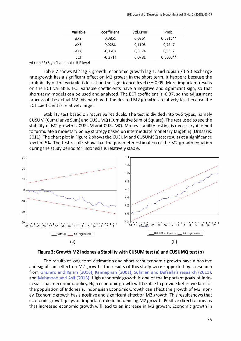
Table 7 shows M2 lag 3 growth, economic growth lag 1, and rupiah / USD exchange rate growth has a significant effect on M2 growth in the short term. It happens because the probability of the variable is less than the significance level α = 0.05. More important results on the ECT variable. ECT variable coefficients have a negative and significant sign, so that short-term models can be used and analyzed. The ECT coefficient is -0.37, so the adjustment process of the actual M2 mismatch with the desired M2 growth is relatively fast because the ECT coefficient is relatively large.

Stability test based on recursive residuals. The test is divided into two types, namely CUSUM (Cumulative Sum) and CUSUMQ (Cumulative Sum of Square). The test used to see the stability of M2 growth is CUSUM and CUSUMQ. Money stability testing is necessary deemed to formulate a monetary policy strategy based on intermediate monetary targeting (Dritsakis, 2011). The chart plot in Figure 2 shows the CUSUM and CUSUMSQ test results at a significance level of 5%. The test results show that the parameter estimation of the M2 growth equation during the study period for Indonesia is relatively stable.

Figure 3: Growth M2 Indonesia Stability with CUSUM test (a) and CUSUMQ test (b)

The results of long-term estimation and short-term economic growth have a positive and significant effect on M2 growth. The results of this study were supported by a research from Ghumro and Karim (2016), Kannapiran (2001), Suliman and Dafaalla’s research (2011), and Mahmood and Asif (2016). High economic growth is one of the important goals of Indo-nesia’s macroeconomic policy. High economic growth will be able to provide better welfare for the population of Indonesia. Indonesian Economic Growth can affect the growth of M2 mon-ey. Economic growth has a positive and significant effect on M2 growth. This result shows that economic growth plays an important role in influencing M2 growth. Positive direction means that increased economic growth will lead to an increase in M2 growth. Economic growth in

(a) (b)

76


Indonesia if experiencing an increase will encourage an increase in people’s income. The high-er the level of income of the people of Indonesia, the demand for money in Indonesia will in-crease, because the increase in income of the Indonesian people will lead to greater economic transactions and this requires the Indonesian people to hold more money. Indonesia’s current economic growth is relatively good, causing credit to be quite smooth. Business people and corporations, as well as the Indonesian people, increase their activities so that the demand for investment credit and working capital increases. This will encourage an increase in M2 in Indonesia. The increase in investment credit is due to easy bank lending, low lending rates, and low credit approval fees. The stability of Indonesia’s economic growth can be realized by maintaining Indonesia’s exports, maintaining fiscal sustainability, preventing price wars and maintaining the investment climate.

The estimation results show that the rupiah/USD exchange rate has a positive and significant effect on the growth of Indonesian M2 in the long and short term. The estimation results show that the rupiah/USD exchange rate plays a role in influencing the growth of M2 Indonesia. The results of this study were supported by research Ghumro and Karim (2016), Suliman and Dafaalla research (2011), and Mahmood and Asif (2016). The positive sign of the rupiah/USD exchange rate coefficient shows the effect of wealth, which means that the depre-ciation of the rupiah/USD will increase the value of foreign assets. Indonesia maintains wealth by selling foreign assets and buying domestic assets because domestic assets are cheap, so domestic money demand increases. Many people in Indonesia have foreign currencies, espe-cially dollars. Many people in Indonesia save a lot of dollars aimed at increasing wealth. The advantage of saving foreign currencies, especially the dollar, is to maintain purchasing power when the rupiah falls. When the dollar is stronger than the rupiah, the Indonesian people choose to sell dollars, because it has a higher return than the initial value when purchased. This condition causes high rupiah demand. The stability of the rupiah / USD exchange rate needs to be done, then policies that need to be implemented for example increasing the BI rate, increasing potential exports, supplying foreign exchange, and buying back government securities from the secondary market.

The estimation results show that interest rates have no significant effect on the de-mand for money in Indonesia. Interest rates do not have a significant effect on money demand indicating that interest rates are insensitive in influencing money demand. This is in line with the theory expressed by Friedman. Interest rates are insensitive to the demand for money Indonesia because competition between banks in Indonesia makes the opportunity to hold money relatively constant. The cause of interest rates is insensitive because interest rates are low, business people and corporations do not prioritize interest rates. For example corpo-rations, investment by corporations that have high productivity are relatively insensitive to interest rates because the corporations have high profits, does not have a significant impact on the company’s cash flow. Household consumption also has no significant effect on the de-mand for money in Indonesia.

The household consumption is the expenditure of goods or services by households to meet needs. The needs of human life are increasing and increasing following the move-ment of time. Human basic needs which include primary needs, secondary needs, and tertiary needs must be realized for survival. Household consumption and money demand also have a relationship. If the Indonesian people estimate their future to be good, then they will feel freer to consume, so consumption expenditure tends to increase and the growth in demand for money also increases. Conversely, if the Indonesian people estimates that their future is bad, they reduce consumption and choose to save, so that the growth in money demand also decreases. These results mean that household consumption has less role in influencing M2

77


growth. This is because the policies of the Indonesian government are directed at reducing the rate of growth in household consumption. The Indonesian government carries out policies such as increasing taxes on individual, institutional or corporate taxpayers. The Indonesian government, through the Minister of Finance, also decided to increase income tax on 1,147 types of imported goods, mainly imports of consumer goods. These policies can reduce the growth of household consumption. Declining growth in household consumption will reduce the growth in M2 money demand.

Figure 4: Velocity of Broad Money in Indonesia Period 2000Q1-20017Q4

The velocity of money in Indonesia done by Bank Indonesia starts from printing new money and distributing it to all BI offices both the central office and regional offices. Further-more, the central BI office and regional offices distribute money through banking and oth-er services. Commercial banks receive money from BI and serve the public’s needs for cash afterwards the public takes money from the bank and uses it for transactions and deposits excess cash to the bank. Banks receive cash deposits from the public and deposit them back to BI. Finally, BI destroys bad money and redistributes new money to be used. Figure 3 shows that Indonesia’s velocity of broad money has an increasing trend during the 2000Q1-2017Q4 period. Increasing the velocity of broad money means that Indonesia’s economic activities are growing. The velocity of broad money in Indonesia has a rising trend which means that the use of money in the hands of people grows so fast and people prefers to spend it instead of saving or investing.

Conslusion

The study concludes that economic growth and the growth of the rupiah / USD ex-change rate have a positive significant effect on M2 growth. However, real interest rates and growth in household consumption have no significant effect on M2 growth in the long term. The variable growth of M2 lag 3, economic growth lag 1, and rupiah/USD exchange rate growth has a significant effect on M2 growth in the short term. Furthermore, the velocity of money in Indonesia is found to have an increased trend.

References

Altayee, H. H. A., & Adam, M. H. M. (2012). Financial Development and the Velocity of Money Under Interst-Free Financing System: An Empirical Analysis. American Based Research Journal, 2(8), 53–65.

BI. (2010). Laporan Kebijakan Moneter 2010 Kuartal IV. Jakarta.

78


BI. (2013). Laporan Kebijakan Moneter 2013 Kuartal IV. Jakarta.

Bitrus, Y. P. (2011). The determinants of the demand for money in developed and developing countries. Journal of Economics and International Finance, 3(15), 771–779. https://doi.org/10.5897/JEIF11.118.

Dritsakis, P. N. (2011). Demand for money in Hungary: An ARDL approach. Aca-demic Research Centre of Canada. https://doi.org/10.1227/01.NEU.0000349921.14519.2A.

Ghumro, N., & Karim, M. Z. A. (2016). The effects of exchange Rate on Money demand : Evi-dence from Pakistan The effects of exchange Rate on Money demand : Evidence from Pakistan. International Research Journal of Social Sciences, 5(4), 11–20.

Habibi, F., & Rahim, K. A. (2009). A Bound Test Approach to Cointegration of Tourism Demand. American Journal of Applied Sciences, 6(11), 1924–1931.

Halıcıoğlu, F., & Uğur, M. (2005). On Stability of the Demand for Money in a Developing OECD Country: The Case of Turkey. Global Business and Economic Review, 7(3), 1–15.

Harb, N., & Hussain, M. N. (2014). Money demand function in SAARC countries. International Journal of Economics and Business Research, 7(4), 444–453. https://doi.org/10.1504/IJEBR.2014.062907.

Havi, E. D. K., Enu, P., & Opoku, C. D. K. (2014). Demand for Money and Long Run Stability in Ghana : Cointegration Approach. European Scientific Journal, 10(13), 483–497.

Kannapiran, C. a. (2001). Stability of Money Demand and Monetary Policy in Papua New Guin-ea (PNG): an Error Correction Model Analysis. International Economic Journal, 15(3), 73–84. https://doi.org/10.1080/10168730100080020.

Kothari, C. R. (2004). Research Methodology: Methods and Techniques (Second Revised Edi-tion). New Delhi: New Age International.

Mahmood, H., & Asif, M. (2016). An empirical investigation of stability of money demand for GCC countries. International Journal of Economics and Business Research, 11(3), 274–286. https://doi.org/10.1504/IJEBR.2016.076177.

Mall, S. (2013). Estimating a Function of Real Demand for Money in Pakistan : An Application of Bounds Testing Approach to Cointegration, 79(5), 32–50.

Mishkin, F. S. (2004). The economics of money, banking, and financial markets. New York: Pearson The Addison Wesley.

Odior, E. S. O., & Alenoghena, R. O. (2016). Empirical Verification of Milton Friedman’s Theo-ry of Demand for Real Money Balancesin Nigeria: Generalized Linear Model Analysis. Journal of Empirical Economics, 5(1), 35–50.

Omer, M. (2014). Velocity of Money Functions in Pakistan and Lessons for Monetary Policy Ve-locity of Money Functions in Pakistan and Lessons for Monetary Policy. SBP Research Bulletin.

Rami, G. (2010). Velocity of Money Function for India: Analysis and Interpretations. SSRN Elec-tronic Journal, 1(1), 15–26. https://doi.org/10.2139/ssrn.1783473.

79


Sahadudheen. (2012). Demand for money and exchange rate: Evidence for wealth effect in India.

Sichei, M. M., & Kamau, A. W. (2012). Demand For Money: Implications for The Conduct of Monetary Policy in Kenya. International Journal of Economics and Finance, 4(8), 72–82. https://doi.org/10.5539/ijef.v4n8p72.

Singh, R., & Kumar, S. (2010). Some empirical evidence on the demand for money in the Pa-cific Island countries. Studies in Economics and Finance, 27(3), 211–222. https://doi.org/10.1108/10867371011060045.

Suliman, S. Z., & Dafaalla, H. A. (2011). An econometric analysis of money demand function in Sudan, 1960 to 2010. Journal of Economics and International Finance, 3(16), 793–800. https://doi.org/10.5897/JEIF11.122.

Suseno, & Solikin. (2002). UANG : Pengertian, Penciptaan, dan Peranannya dalam Perekono-mian. Jakarta: Bank Indonesia. https://doi.org/10.1038/cddis.2011.1.

Widarjono, A. (2013). Ekonometrika Pengantar dan Aplikasinya Disertai Panduan Eviews. Yog-yakarta: UPP STIM YKPN.

determinants of demand for money and the velocity …

Documents