detection of intraventricular …ufdcimages.uflib.ufl.edu/uf/e0/04/20/36/00001/tang_t.pdfdetection...
TRANSCRIPT

1
DETECTION OF INTRAVENTRICULAR HEMORRHAGE IN NEONATES USING ELECTRICAL IMPEDANCE TOMOGRAPHY
By
TE TANG
A DISSERTATION PRESENTED TO THE GRADUATE SCHOOL OF THE UNIVERSITY OF FLORIDA IN PARTIAL FULFILLMENT
OF THE REQUIREMENTS FOR THE DEGREE OF DOCTOR OF PHILOSOPHY
UNIVERSITY OF FLORIDA
2010

2
© 2010 Te Tang

3
To my family in China

4
ACKNOWLEDGMENTS
First and foremost, if there is only one person in this world that deserves all my
gratitude in the past five years, this person is Dr. Rosalind Sadleir. I appreciate that she
offered me this opportunity to research in the field of Electrical Impedance Tomography
and her continuous support for my whole 5-year Ph. D. study. I could have achieved
nothing without her guidance, patience and instruction in the ways of the research world
along the journey. Year 2005 – 2010 was definitely a turning point in my career. I will
never forget this pleasant and valuable experience in my entire life.
I want to say thank you to many other people, especially my committee members,
Dr. Johannes van Oostrom, Dr. David Gilland and Dr. Stephen Blackband, for offering
good advice at critical points along the way. I would like to give specials thanks to Dr.
Peggy Borum and Dr. Michael Weiss for their help on the piglet experiments. The in
vivo animal experiments would not be a possibility without their professional assistance.
I hope we can continue our corporation in the following stage of this project. I would also
like to thank my lab mates, Sungho Oh and Aaron Tucker. They have contributed to the
completion of my work in significant ways.

5
TABLE OF CONTENTS page
ACKNOWLEDGMENTS ...................................................................................................... 4
LIST OF TABLES ................................................................................................................ 9
LIST OF FIGURES ............................................................................................................ 10
ABSTRACT........................................................................................................................ 14
CHAPTER
1 INTRODUCTION ........................................................................................................ 16
Electrical Impedance Tomography ............................................................................ 16 Development and Applications ............................................................................ 16
Intraventricular Hemorrhage....................................................................................... 17 What Is IVH .......................................................................................................... 17 Current Modalities for the Monitoring and Treatment of IVH .............................. 18 Potential of Electrical Impedance Tomography .................................................. 19
Organization of the Dissertation ................................................................................. 22
2 EIT METHODS ........................................................................................................... 25
EIT Forward Problem ................................................................................................. 25 Formulation of Forward Problem ......................................................................... 25 Formulation of the Finite Element Solution ......................................................... 26 Conjugate Gradient Method................................................................................. 30
EIT Inverse Problem ................................................................................................... 33 Overview............................................................................................................... 33 Formulation of Linearized Algorithm.................................................................... 35 Sensitivity Matrix .................................................................................................. 35 Lead Field Theory ................................................................................................ 37
Regularization of the Inverse Problem ....................................................................... 41 Ill-posed Nature of the Inverse Problem.............................................................. 41 Tikhonov Regularization ...................................................................................... 42 Truncated Singular Value Decomposition (TSVD) ............................................. 42
Singular value decomposition (SVD) ............................................................ 42 Condition number and TSVD ........................................................................ 44 L-curve ........................................................................................................... 45 Weighted minimum norm method ................................................................. 46
Quantitative Measures of EIT Reconstruction ........................................................... 47 Sensitivity and Selectivity ........................................................................................... 48 EIT Hardware .............................................................................................................. 49
3 PIGLET SKULL IMPEDANCE MEASUREMENT ...................................................... 63

6
Background and Significance ..................................................................................... 63 Method ........................................................................................................................ 64
Sample Preparation ............................................................................................. 64 Measurement Apparatus ..................................................................................... 64 Theory .................................................................................................................. 65
Result .......................................................................................................................... 66 Discussion ................................................................................................................... 66 Conclusion .................................................................................................................. 68
4 A ROBUST CURRENT PATTERN FOR THE DETECTION OF IVH ....................... 72
Background ................................................................................................................. 72 Method ........................................................................................................................ 72
Candidate Current Patterns ................................................................................. 72 Sensitivity Studies for the Candidate Current Patterns ...................................... 74 Data Generation ................................................................................................... 76
Finite element models ................................................................................... 76 Phantom models............................................................................................ 77
Reconstruction Method ........................................................................................ 79 Localization of EIT Reconstructions .................................................................... 80 Image Resolution and Contrast ........................................................................... 80 Comparison between ‘Open Skull’ and ‘Closed Skull’ Models ........................... 82
Sensitivity analysis using a layered model ................................................... 82 Noise analysis using model B ....................................................................... 83
Results ........................................................................................................................ 84 Sensitivity and Selectivity for the Uniform Models .............................................. 84 Comparing the Three Current Patterns Using Model A ...................................... 85 Comparing RING and EEG Patterns Using Model B and Phantom Data .......... 86 Comparison between ‘Open Skull’ and ‘Closed Skull’ Models ........................... 87
Discussion ................................................................................................................... 88 Sensitivity and Selectivity .................................................................................... 88 Overall Evaluation with Model A .......................................................................... 89 Model B and Phantom Experiment Results ........................................................ 90 Anomaly Quantification ........................................................................................ 92 Comparison between ‘Open Skull’ and ‘Closed Skull’ Models ........................... 93 Comparing Localization Results with Earlier Studies ......................................... 94 Other Possible Applications ................................................................................. 95
Conclusion .................................................................................................................. 95
5 STUDIES USING A REALISTIC HEAD-SHAPED MODEL .................................... 109
Background ............................................................................................................... 109 Methods .................................................................................................................... 110
The Neonatal Head-shaped Model ................................................................... 110 Sensitivity Analysis............................................................................................. 110 Simulation of IVH ............................................................................................... 111 Investigation of Boundary Shape Mismatch...................................................... 112

7
Forward models ........................................................................................... 112 Data generation ........................................................................................... 112
Results ...................................................................................................................... 115 Sensitivity Analysis............................................................................................. 115 Layered RG Model ............................................................................................. 116 Investigation of Boundary Geometry Effects Using Homogeneous RG
Models ............................................................................................................. 117 Discussion ................................................................................................................. 118 Conclusion ................................................................................................................ 122
6 STUDIES USING PIGLET MODELS ....................................................................... 133
Introduction ............................................................................................................... 133 Methods .................................................................................................................... 133
Piglet 1 ................................................................................................................ 133 Piglet 2 and 3 ..................................................................................................... 134 Piglet 4 (the MRI Piglet) ..................................................................................... 135 Piglet 5 ................................................................................................................ 137 Piglet 6 ................................................................................................................ 137 Piglet 7 and 8 ..................................................................................................... 138 Piglet 9 and 10 ................................................................................................... 138
Results ...................................................................................................................... 139 Piglet 1 ................................................................................................................ 139 Piglet 2 and 3 ..................................................................................................... 139 Piglet 4 ................................................................................................................ 140 Piglet 5 and 6 ..................................................................................................... 140 Piglet 7 and 8 ..................................................................................................... 141 Piglet 9 and 10 ................................................................................................... 141 Summary ............................................................................................................ 142
Discussion ................................................................................................................. 143 Conclusion ................................................................................................................ 146
7 SUMMARY ................................................................................................................ 163
Conclusion ................................................................................................................ 163 Future Work .............................................................................................................. 165
Improving in vivo Animal Experiment ................................................................ 165 Improving the Measurement Strategy ............................................................... 165
APPENDIX
A USEFUL C++ CODE FOR CONJUGATE GRADIENT METHOD .......................... 167
Bracket the Minimum ................................................................................................ 167 Search for the Minimum ........................................................................................... 168 Line Minimization ...................................................................................................... 170 Conjugate Gradient Method ..................................................................................... 170

8
B PROCEDURES FOR IN VIVO PIGLET EXPERIMENTS ....................................... 172
LIST OF REFERENCES ................................................................................................. 177
BIOGRAPHICAL SKETCH.............................................................................................. 188

9
LIST OF TABLES
Table page 1-1 Estimates of the conductivity (S/m) of body tissues below 100 Hz at body
temperature (Gabriel et al. 1996) .......................................................................... 23
1-2 Grades of Intraventricular hemorrhage defined by Papile et al. (1978), with associated risks and ultrasound specificities ........................................................ 24
3-1 Measurement results for the fresh skull samples.................................................. 70
3-2 Measurement results for the frozen skull samples................................................ 71
4-1 Spherical coordinates of EEG electrodes, in degrees. T7 is left temporal and T8 right temporal. Oz is Occipital central electrode. ............................................. 96
4-2 The condition number, rank and size for the sensitivity matrix used for each current pattern and truncation point chosen for each case ................................ 101
4-3 Comparison of resolutions R calculated for each of the cases shown in Figure 4-14 ........................................................................................................... 106
5-1 Resolution values of the reconstructions for all the anomaly volumes. ............. 132
6-1 Linear Discriminant Analysis (LDA) for all the in vivo piglet QI data .................. 162
10
LIST OF FIGURES
Figure page 1-1 Intraventricular Hemorrhage (IVH). ....................................................................... 24
2-1 A domain with 4 boundaries divided into elements. .............................................. 54
2-2 A tetrahedral element ............................................................................................. 54
2-3 Demonstration of a dipole source within a volume conductor. ............................. 55
2-4 The lead field distribution within a 2D elliptical domain. ....................................... 55
2-5 Illustration of the reciprocity theorem of Helmholtz ............................................... 56
2-6 Derivation of the equation for lead field theory. .................................................... 56
2-7 Singular values of the sensitivity matrix for the homogeneous spherical model with EEG current pattern............................................................................. 57
2-8 L-curve examples using different regularization algorithm. .................................. 57
2-9 A comparison between un-weighted and weighted 2D reconstructions. ............. 58
2-10 The first and second generation of Epack EIT systems. ...................................... 58
2-11 Comparison of aperture times in EPack1 and EPack2. ........................................ 59
2-12 Overall system design of the EPack1 system ....................................................... 59
2-13 Schematic of the EPack module. ........................................................................... 60
2-14 The EPack module, showing battery pack (top right), main acquisition board (center) and electrode connections (center) ......................................................... 61
2-15 EPack software screenshot (left). Amplified reconstructed image (top right). Phantom experiment using a full-array electrode configuration (bottom right). ... 62
3-1 Skull sample preparation, showing the left frontal, left parietal, right frontal and right parietal bone samples............................................................................. 69
3-2 The measurement cell used to measure skull impedance. .................................. 69
3-3 Skull conductivities plotted as a function of their thickness. ................................. 71
4-1 Three electrode configurations viewing from the top and demonstrations of the current pattern applied in each case. .............................................................. 96

11
4-2 Forward models with three different electrode layouts. ........................................ 97
4-3 Three-dimensional EEG spherical models showing central and lateral ventricle regions. .................................................................................................... 97
4-4 A model with an outer brain shell and a central region of CSF (Model A) viewing from the top. .............................................................................................. 98
4-5 A more complex model (Model B) with scalp, brain, ventricles and skull shells, including a structure similar to the fontanel (highlighted). ......................... 98
4-6 MRI images of a neonatal head, from which we determined the position and size of the ventricles. .............................................................................................. 99
4-7 Spherical phantoms with EEG layout (left) and RING layout (right)................... 100
4-8 The complete phantom experiment system ........................................................ 100
4-9 Layered spherical model with EEG layout. ......................................................... 101
4-10 Average sensitivities, calculated as a fraction of maximum values observed over the domain, for EEG, Cz-RING and RING patterns in the regions of interest. ................................................................................................................. 102
4-11 Absolute selectivities observed within a relatve radius 0.8≤ , for EEG, Cz-RING and RING patterns in the regions of interest. ........................................... 103
4-12 Radial relative localization errors for simulations on model A. ........................... 104
4-13 Quantification Indices of the 37 different anomaly positions for each of the three current patterns on model A. ...................................................................... 104
4-14 Axial (relative radial position z = 0.3) and sagittal (x = -0.2) cross sections (first and second columns) and isosurfaces (third column) of an blood-like anomaly in each case. ......................................................................................... 105
4-15 Radial relative localization errors Dxy and Dz of the 6 anomaly positions for simulated (model B) and phantom data for RING and EEG patterns. ............... 106
4-16 Quantification Indices of the six anomaly positions with simulated (model B) and phantom data for the RING and EEG patterns. ........................................... 107
4-17 Comparisons between ‘open-skull’ and ‘closed-skull’ reconstructions. ............. 108
5-1 The 3D neonatal head model visualized using Pro ENGINEER (Parametric Technology Corp.). ............................................................................................... 123
5-2 The neonatal head model visualized using Comsol 3.4, showing the anatomical structures and scalp electrode configuration. ................................... 123

12
5-3 Axial, saggital and coronal views of realistic geometry model, showing ventricular and central structures. ....................................................................... 124
5-4 The two ventricle structures (red dots) added within the brain, and the six anomaly positions (blue dots) within the ventricles. ............................................ 124
5-5 The three models used for data generation. ....................................................... 125
5-6 Procedures of constructing a head-shaped phantom. ........................................ 125
5-7 One slice (#74) of the original Gent model MRI data, showing the five major structures in the head........................................................................................... 126
5-8 Dividing a rectangular brick element (1234-5678) into six tetrahedral elements, which are: 1245, 2456, 2346, 3678, 3468 and 4568. ........................ 126
5-9 Sensitivities and selectivities found in the regions of interest using a uniform RG sensitivity matrix. ........................................................................................... 127
5-10 Comparisons between reconstructions using SPS and RGS matrix. .................... 128
5-11 Image and conductivity profile in reconstructions of different anomaly pairs..... 129
5-12 Quantification Indices (with the corresponding volume estimation labeled on the right) for the multi-site bleeding cases using SPS and RGS . .......................... 130
5-13 Comparison of average QI errors (with the corresponding errors in volume estimation labeled on the right) for the 63 cases using the two sensitivity matrices under 11 different SNR levels ranging from 60 dB to 90 dB. .............. 130
5-14 Reconstructions with the RG matrix and SP matrix using the data from the four models. .......................................................................................................... 131
5-15 Quantification indices for the images reconstructed with the RG matrix and SP matrix. ............................................................................................................. 132
6-1 The piglet head and electrode configuration used on piglet 1. ........................... 147
6-2 Electrodes and artificial brain used for piglet 1 experiment. ............................... 147
6-3 Experiment setup for piglet 2. .............................................................................. 148
6-4 Experiment setup for piglet 3. .............................................................................. 148
6-5 Piglet 4 (The MRI piglet). ..................................................................................... 149
6-6 The injection guide designed to assist introducing the canula into the ventricle. ............................................................................................................... 149

13
6-7 Post mortem experiment on piglet 4. ................................................................... 150
6-8 Difference voltage measurements generated by the two 4ml saline injections on piglet 1. ............................................................................................................ 150
6-9 Isosurface plots of reconstructions of injections to the closed skull piglet (piglet 2). ............................................................................................................... 151
6-10 Quantification index as a function of injected saline volume for piglet 2. ........... 152
6-11 Isosurface plots of reconstructions of injections to the right open piglet skull (piglet 3). ............................................................................................................... 152
6-12 Quantification index as a function of injection time for piglet 3........................... 153
6-13 Isosurface plots of reconstructions of injections to the right side on piglet 4 (the intact MRI piglet). .......................................................................................... 153
6-14 Quantification index as a function of injection time for piglet 4........................... 154
6-15 Signals recorded in one of the measurements for piglet 5 and 6. ...................... 154
6-16 Coronal brain slices of piglet 6............................................................................. 155
6-17 QI values and reconstructed images for in vivo experiment on piglet 7............. 156
6-18 QI values and reconstructed images for in vivo experiment on piglet 8............. 157
6-19 Brain slices taken in coronal planes for piglet 7. ................................................. 158
6-20 Brain dissection for piglet 8. ................................................................................. 159
6-21 Results for in vivo experiment on piglet 10. ........................................................ 160
6-22 Brain dissection for piglet 10. ............................................................................... 161
6-23 Linear fits between the QI values and injected volumes for all the available piglet experiment data. ......................................................................................... 162
B-1 Experiment picture showing the setups for the umbilicus catheter. ................... 175
B-2 Setup for blood injection ...................................................................................... 176

14
Abstract of Dissertation Presented to the Graduate School of the University of Florida in Partial Fulfillment of the Requirements for the Degree of Doctor of Philosophy
DETECTION OF INTRAVENTRICULAR HEMORRHAGE IN NEONATES USING
ELECTRICAL IMPEDANCE TOMOGRAPHY By
Te Tang
August 2010
Chair: Rosalind J. Sadleir Major: Biomedical Engineering
Electrical impedance tomography (EIT) is a medical imaging technique in which
images of conductivity within a body can be inferred from surface electrode
measurements. EIT has been studied in different clinical areas such as brain imaging,
thorax imaging and breast imaging. The focus of this thesis is to investigate the
feasibility of EIT on the detection of intraventricular hemorrhage in premature neonates.
Cerebral intraventricular hemorrhage (IVH) in neonatal human infants is a
common consequence of pre-term delivery. It is currently assessed using ultrasound,
MRI or CT scan. These modalities are not suitable for continuous monitoring of infants
and involve large personnel or equipment costs. Because blood has a high electrical
conductivity contrast relative to other cranial tissue, its appearance can be detected and
monitored using electrical impedance methods. EIT is a non-invasive, low-cost
monitoring alternative to these imaging modalities, and has the potential to measure
bleeding rate and approximately localize the bleeding site.
The first part of this work aimed to find a robust current pattern for the detection of
IVH. We proposed three different electrode layouts and current patterns (RING, EEG
and Cz-RING patterns), and compared their performance using a homogeneous

15
spherical head model. Sensitivity analysis shows that the EEG current pattern has
larger absolute selectivities than the RING and Cz-RING patterns in all the regions of
interest. Numerical simulation and saline phantom experiments also show that the
reconstructed images using the EEG pattern have better image qualities and
quantification accuracies in general.
The second part of this study involved numerical simulations and phantom
experiments using models with realistic boundary geometry. We investigated the
advantage and disadvantage of using a sensitivity matrix calculated from a
homogeneous realistic geometry model (the RG matrix). We found that the RG matrix
does not always produce better image quality than the spherical matrix when there is a
model mismatch in boundary geometry. In addition to that, the RG matrix does not show
any advantage in terms of quantification accuracy. Therefore, we decided that using the
spherical sensitivity matrix would be a better choice for applications on real subjects.
Finally, post mortem and in vivo experiments were conducted on piglets to validate
our method. We were able to detect 0.2 ml saline injections in post mortem piglets and
quantify the accumulative blood volumes with consistent accuracy. We successfully
detected 0.5 ml blood injections in live animals. The quantification results are consistent
for all the in vivo experiments. The reconstructed images of blood volumes are
confirmed by the brain slices after each experiment. All the results indicate that EIT will
be an effective method for monitoring intraventricular bleeding in neonates.

16
CHAPTER 1 INTRODUCTION
Electrical Impedance Tomography
Development and Applications
Electrical impedance tomography (EIT) is a non-invasive medical imaging
technique in which images of conductivity within a body can be inferred from surface
electrode measurements. In conventional EIT measurements, currents are injected into
a volume through one pair of an electrode array, and the data consists of differential
voltages measured between other array electrodes. EIT is a novel imaging method that
has evolved over the past 20 years. The main goal of EIT is to reconstruct the electrical
conductivity distribution as a physiologically useful image, which is possible because the
voltage measurements depend on the conductivity distribution within the object.
Originally, EIT was not developed for clinical applications. The first use of EIT was
reported in 1930 on geological studies (Stephanesco and Schlumberger 1930). People
today are still using EIT for industrial purposes, such as detecting air bubbles in process
pipes (Ljaz et al. 2008) and landmine detections (Wort et al. 1999). The fact that
different human tissues have different electrical properties (Stoy et al. 1982) indicated
the possibility of using EIT for clinical applications. Table 1-1 listed the conductivity of
different human tissues at low frequency. It has been more than 20 years since the
Sheffield group produced the first clinical images using EIT in the year 1987 (Brown and
Seager 1987). However, EIT has not been routinely used in daily clinical practice.
People should face the difficulty that EIT does not have a good spatial resolution as
other commonly used imaging modalities such as Magnetic Resonance Imaging (MRI)
and Computer Tomography (CT). The spatial resolution is related to the number of

17
electrodes used. There are practical problems applying a large number of electrodes,
due to the complexity of electronics and the computational difficulties to process a large
quantity of data (Rahim et al. 2003). However, EIT is much cheaper than the
conventional imaging techniques and requires no ionizing radiation. Another advantage
of EIT is its temporal resolution. It is capable of producing multiple images within a
second. In addition to that, the EIT system can be easily made portable using a laptop
or even a PDA (Tang et al. 2006). All these advantages made EIT a promising bedside
tool in clinical use for the purpose of continuous monitoring.
EIT has potentials on a range of clinical applications. We can summarize the
research in different clinical areas into the following categories:
• Pulmonary function (Holder and Temple 1993, Brown et al. 1995, Cheney et al. 1999, Mueller et al. 2001)
• Thoracic blood volume (Eyuboglu et al. 1987, Mueller et al. 2001, Hoetink et al. 2002)
• Breast tumors (Cherepenin et al. 2002, Kerner et al. 2002, Glickman et al. 2002)
• Hyperthermia (Foster and Schwann 1989, Liu and Griffiths 1993, Moskowitz et al. 1995)
• Gastrointestinal function (Mangnall et al. 1987, Mangnall et al. 1991, Akkermans and Tekamp1993, Nour et al. 1995)
• Internal bleeding (Meeson et al. 1995, Sadleir and Fox 1998, Sadleir and Fox 2001, Xu et al. 2007)
• Brain Imaging (Holder et al. 1996, Rao et al. 1997, Tidswell et al. 2001a, b, c)
Intraventricular Hemorrhage
What Is IVH
While many aspects of birth outcomes have been vastly improved worldwide in the
last 50 years, preterm birth is still the major cause of poor birth outcome (Goldenberg

18
and Jobe 2001) and more than 50% of infants born at 24 weeks’ or less gestation will
die. Although survival rates of preterm infants have increased markedly, survivors of
neonatal intensive care units suffer high rates of neurodevelopmental disability such as
cerebral palsy and sensory impairment. Handicap rates for very low birth weight
(VLBW) preterm infants are high: more than 50% of infants with a birth weight of 1kg or
less are educated in special education environments (Ment et al. 2002). A common
cause of such disabilities is hemorrhage, hypoxia or ischemia in the neonatal brain.
Incidence of premature births is also increasing (from 9.5% in 1980 to 11% in 1998)
partly as a consequence of infertility treatment and associated multiple births
(Goldenberg and Jobe 2001). Intra-ventricular hemorrhage (IVH) (Figure 1-1) affects
35-50% of premature human infants who are born at 32 weeks’ gestation and below
(York and DeVoe 2002), and is a major cause of death and disability. Papile et al.
(1978) classified intra-ventricular hemorrhage into four grades (Table 1-2). Grades I and
II are rarely associated with morbidity or permanent incapacity. Grades III and IV are
associated with increased morbidity (nearly uniform morbidity in the case of Grade IV),
conditions such as cerebral palsy (CP), periventricular leukomalacia (PVL) and post-
hemorrhagic hydrocephalus (PHH).
Current Modalities for the Monitoring and Treatment of IVH
About 65% of IVH in VLBW preterm infants is detected during the first week, with
most occurring in postnatal days 4-5 (Ment et al. 2002). While serious IVH may be
detected from a bulging fontanel, or encephalopathy of the patient, at present, the
conventional diagnosis method for newborns at risk of IVH is ultrasound. Additionally,
MRI is increasingly recommended for patients where there is an ambiguity in bleeding
status or in term neonates who have presented with suspicious clinical signs (Hintz and

19
O’Shea 2008). Neither ultrasound, MRI nor CT are suitable for continuous monitoring
use because of their cost, interference with normal patient management or the presence
of ionizing radiation. While many localities are equipped to care for premature infants,
the ability to monitor complications may be compromised by lack of access to more
expensive imaging modalities such as MRI. Ultrasound is 76-100% specific in at
detection of grade I lesions of greater than 5mm width and almost 100% specific in
grade III or IV hemorrhage. However, US detection of grade II hemorrhages (free blood
in normal sized ventricles) is much less accurate (Babcock et al. 1982, Mack et al.
1981). Over the last decade, results have been presented that demonstrate early testing
of Optical Tomography (NIRS, OT or OCT) in monitoring IVH (Austin et al. 2006). Other
workers are involved in evaluation of IVH detection methods using PET, SPECT and
fMRI (Ment et al. 2002), all in initial stages. Serial lumbar punctures or placement of a
permanent ventroperitoneal shunts may be required to relieve posthemorrhagic
hydrocephalus subsequent to confirmed grade III or IV IVH (York and DeVoe 2002).
Glucocorticoid drugs may be administered to mature the tissue if patient shows
abnormal signs. Low-dose indomethacin (Ment 1994), steroids or glutamine therapy
may also be used as IVH preventatives or therapies (Anon 2004). As treatments
become available, early warning of IVH becomes crucial.
Potential of Electrical Impedance Tomography
EIT monitoring involves the application of an electrode array (typically 16 to 32
electrodes) over the surface of an area of interest (Boone et al. 1997, Cheney et al.
1999). Sequences of current patterns are applied to a subset of electrodes, and
voltages produced by the applied currents are measured. The currents employed are
high frequency (ca. 50 kHz) and at a low enough magnitude that they are harmless.

20
These measurements are used to create a cross-sectional map of electrical impedance.
Measurements can typically be made and images reconstructed rapidly. As mentioned
earlier, although EIT images have relatively poor spatial resolution compared to
modalities such as MRI and CT, they nevertheless contain valuable physical
information, and can be collected with little cost. By comparing data collected at an
earlier time to those collected at the current time, images of impedance change, and
therefore, rates, of processes may be identified. Blood is generally easily detectable in
the body because free blood has a significant impedance contrast with other tissues
and fluids (Geddes and Baker 1967, Faes et al. 1999). Determining absolute
conductivity values is considerably more difficult and is hindered by other problems
such as unknown boundary shape, and the need to estimate electrode contact
impedances. The major advantage of EIT in clinical situations is that it is non-invasive
and not operator dependent. It may also be used in nurseries in remote areas or as a
monitoring tool during transfer to larger care facilities. EIT may be a good alternative to
ultrasound as a screening tool to monitor and alert clinicians to the presence and
progress of bleeding, an increasingly important utility as therapies for IVH become
available (Hansen 2006).
The application of EIT to detect bleeding in the head is potentially useful because
of the conductivity changes that occur as the result of bleeding, but suffers the
disadvantage of being hindered by the poorly conductive skull and highly conductive
CSF. The skull is always a big problem when using scalp electrodes because the scalp
which is relatively more conductive tends to shunt the current away from the skull.
Therefore the amount of current that actually enters the skull is very limited. Phantom

21
experiments performed by the UCL group demonstrated that the presence of a skull
could reduce the impedance change to one fifth that observed without the skull
(Tidswell et al. 2001b). For the same reason, the CSF layer existing between the skull
and brain also tends to shunt current away from the brain. The CSF in the ventricles
also shunts current away from the blood, which makes the overall impedance change
caused by bleeding relatively smaller. All these shunting effects make the detection of
bleeding difficult. The ultimate goal of this study is to develop and test a reconstruction
method in a piglet head model in order to form 3D images of electrical conductivity
inside the neonatal head. EIT was briefly tested to the detection of neonatal intra-
ventricular hemorrhage in the late 1980s (Murphy et al. 1987, McArdle et al. 1988), with
a result showing detection of ventricular bleeding in one neonatal patient. These data
were, however, significantly affected by artifacts. Murphy et al. (1987) found that
breathing movements and variations in cerebral blood flow caused the largest signal
artifacts – up to 1% variation in their baseline signal at a frequency of approximately 0.5
Hz. The other significant artifact was synchronous with heart electrical activity, causing
a variation of about 0.1% in signals. Large artifacts due to movement of the infant were
also encountered. Nevertheless, these early studies of IVH using EIT demonstrated the
potential of EIT for this application. More recently, EIT has also been applied to
detection of brain activity, stroke and epilepsy (Tidswell et al. 2001a, b, c, Liston 2004).
Their studies have indicated the possibility of using EIT as an imaging tool in
circumstances where blood volume changes occur in the brain.

22
Organization of the Dissertation
The goal this dissertation is to detect and quantify intraventricular bleeding in a
piglet model. One future goal is to make this application available as a routine clinical
procedure on neonates.
The dissertation is organized as follows. In Chapter 1 we gave a literature review
of EIT applications. Then, we pointed out the significance of IVH, which led us to the
ultimate goal of this study. In Chapter 2 we review two important aspects of EIT,
mathematics and hardware and introduce the algorithms used in this work. Piglet skull
impedance measurements are discussed in Chapter 3. The measurement results were
important for us to choose a proper skull parameter in the simulations for neonates. We
demonstrate in Chapter 4 the first step of this work, which was finding a robust current
pattern for this application using spherical models. The advantage of the current pattern
on a neonatal application was analyzed based on the results from numerical simulation
and phantom experiments. In Chapter 5 we further investigate this current pattern using
more complicated models with realistic boundary geometries, showing that using a
homogeneous spherical forward model is consistent in terms of quantification. Chapter
6 contains the details of animal experiments on piglet models. Both post mortem and in
vivo experiments were conducted. We show that we were able to detect blood volumes
as low as 0.2 ml and that the bleeding process can be quantified consistently using a
homogeneous spherical forward model.

23
Table 1-1. Estimates of the conductivity (S/m) of body tissues below 100 Hz at body temperature (Gabriel et al. 1996)
Tissue Conductivity Bladder 0.2 Bone -Cancellous 0.07 Bone -Marrow 0.05 Cartilage 0.18 Cerebro Spinal Fluid 2.0 Cornea 0.4 Fat 0.04 Gall Bladder Bile 1.4 Heart 0.1 Lens 0.25 Lung -Deflated 0.2 Muscle 0.35 Pancreas 0.22 Small Intestine 0.5 Stomach 0.5 Testis 0.4 Tongue 0.3 Blood 0.7 Bone –Cortical 0.02 Breast 0.06 Cerebellum 0.1 Colon 0.1 Dura 0.5 White matter 0.06 Grey matter 0.1 Kidney 0.1 Liver 0.07 Lung –Inflated 0.08 Nerve 0.03 Skin –Wet 0.1 Spleen 0.1 Tendon 0.3 Vitreous Humour 1.5 Thyroid 0.5

24
A B
Figure 1-1. Intraventricular Hemorrhage (IVH). A) A sagittal view of head anatomy, showing the ventricles, B) Pictures showing the four IVH grades.
Table 1-2. Grades of Intraventricular hemorrhage defined by Papile et al. (1978), with associated risks and ultrasound specificities
Grade Description Consequences Detection I Isolated germinal matrix
hemorrhage with no extension to the ventricles
Unlikely to lead to morbidity and disability
75% of cases detectable using ultrasound
II Intraventricular hemorrhage with normal ventricular size; blood occupies up to 50% of the of the ventricular volume
Unlikely to lead to morbidity and disability alone
50% of cases detectable using ultrasound
III Intraventricular hemorrhage with ventricular dilatation; blood occupies more than 50% of the ventricular volume
Increased risk of CP, PHH and PVL. Morbidity possible
75%-100% of cases detectable using ultrasound
IV Intraventricular hemorrhage with parenchymal involvement; ventricles often dilated.
Increased risk of CP, PHH and PVL. High risk of morbidity
75%-100% of cases detectable using ultrasound

25
CHAPTER 2 EIT METHODS
EIT Forward Problem
Formulation of Forward Problem
The world of electromagnetic fields is governed by Maxwell’s equations which
relate the electric and magnetic fields to their sources, charge density and current
density. To formulate the EIT forward problem, we firstly need to reduce the complexity
by making the assumption that EIT is an electrostatic system. That means the effect
generated from changing magnetic fields can be neglected. Therefore, the equation for
Faraday’s law of induction becomes:
0BEt
∂∇× = − =
∂ (2-1)
Let’s assume that Ω is a three dimensional domain with smooth surfaces.
( , , )x y zσ is the conductivity distribution within the domain. Equation 2-1 implies that, for
a electrostatic system, the electric field E can be written as the gradient of the potential
distribution ( , , )x y zΦ within domain Ω (Equation 2-2).
E = −∇Φ (2-2)
Ampere’s law relates the magnetic field to its electric current source (Equation 2-
3), where H is the magnetic field intensity, fJ is the enclosed conduction current
density and D is the electric displacement field.
fH J Dt
∂∇× = +
∂ (2-3)
J Eσ= (2-4)

26
In an electrostatic system, the term Dt
∂∂
is 0. The current density is related to the
electric field by Ohm’s law (Equation 2-4). By taking the divergence on both sides of
Equation 2-3 then combining with Equation 2-2, we have:
( ) 0σ∇ ∇Φ = in domain Ω (2-5)
Equation 2-5 is exactly the Laplace equation, with Dirichlet boundary condition
vΦ = or Neumann boundary condition ( ) jσ η∂Φ ∂ = , where η∂ ∂ denotes the normal
derivative to the surface. The forward problem in EIT reconstruction is to solve for Φ
with a given conductivity distribution σ .
Formulation of the Finite Element Solution
The forward problem can be solved analytically when the geometry of the domain
is simple (such as a circular shape in 2D and a spherical or cylindrical shape in 3D) and
the conductivity distribution is homogenous or at least simple enough (Pidcock et al.
1995a, Pidcock et al. 1995b, Holder 2004). When the geometry and conductivity
structure become complicated, analytical solutions are generally not available. In most
situations, numerical methods are needed to solve the forward problem, such as the
Finite Element Method (FEM).
Before formulating the FEM solution, we need to introduce two theorems that will
be useful to understand the journey of formulation later on. The first concept is the
functional. The functional is the function that minimizes the energy of a system. For the
system L fφ = , where L is an operator, the functional is written as Equation 2-6. If
operator L is self adjoint and positive definite, the solution of the system is unique and
occurs at the minimum of [ ]I φ .

27
[ ] 2R R
I L dxdy fdxdyφ φ φ φ= −∫∫ ∫∫ (2-6)
Minimization of [ ]I φ can be achieved by applying the Rayleigh-Ritz method. The
Rayleigh-Ritz method is a systematic method to obtain a minimum. In this method the
solution 0φ is approximated as a sum of n linearly independent weighted basis functions
(Equation 2-7). Then the problem is equivalent to finding the value for each ic to
minimize the functional.
01
n
n i ii
cφ φ ψ=
≈ = ∑ (2-7)
Therefore, the functional for the Poisson equation ( 2 fφ−∇ = ) can be written as
Equation 2-8. The Laplace equation is a special case of the Poisson equation when f
is zero.
2 21( ,..., ) ( ) ( ) 2i i
n i i i iR
I c c c c c f dxdyx y
ψ ψ ψ ∂ ∂
= + − ∂ ∂ ∑ ∑ ∑∫∫ (2-8)
So now we have related the solution to the entire domain. The next step is to
divide the domain into elements. Then the solution φ can be discretized to the solutions
on the nodes of the elements 1( ,..., )nφ φ φ= .
For the 2D domain shown in Figure 2-1, let’s assume that the domain has 4
boundaries, C1 to C4. Boundaries C1 and C2 have Dirichlet conditions and boundaries
C3 and C4 have Cauchy conditions. If we apply the Laplace equation ( ) 0k φ−∇ ∇ = to
the domain, the functional can be written as:

28
1 2
3 4
22
1 2
2 21 1 2 2
[ ] 2 ( ) 2 ( )
( 2 ( )) ( 2 ( ))
R C C
C C
I k k dxdy h s ds h s dsx y
g s ds g s ds
φ φφ φ φ
σ φ φ σ φ φ
∂ ∂ = + − − ∂ ∂
+ − + −
∫∫ ∫ ∫
∫ ∫ (2-9)
By applying equation 2-8 to 2-9, we can prove that the functional of the entire
domain is equivalent to the sum of the functionals of the single elements (Equation 2-
10), where E is the total number of elements and eI is the functional of a individual
element.
11
[ ] ( ,..., )E
en
eI I Iφ φ φ
=
= =∑ (2-10)
Therefore, to minimize [ ]I φ , we can use equation 2-11:
10 1,...,
eE
ei i
I I i nφ φ=
∂ ∂= = =
∂ ∂∑ (2-11)
If we look at a single element, the derivative of the functional eI to each iφ can be
written as:
( )2 2
22
e e
e e e ee
i i i i iR C
I k k dxdy hdsx y
φ φ φσ φφ φ φ φ φ
∂ ∂ ∂ ∂ ∂ ∂ ∂ = + + − ∂ ∂ ∂ ∂ ∂ ∂ ∂ ∫∫ ∫ (2-12)
The solution within a single element eφ can be expressed using the element
shape function and the solutions on the element nodes (Equation 2-13).
e( , ) N ...p
e e e e ej j p s
j es
x y N N Nφ
φ φ δφ∈
= = =
∑ (2-13)
eN is the shape function of the element. The shape function is an interpolation
function which interpolates the internal solution within the element using the solutions

29
on the nodes. Substituting Equation 2-13 into 2-12 and reorganizing the equation, we
have a final form for e
i
Iφ
∂∂
(Equation 2-14):
2 2 2 2e
e e e eij j ij j i i
j e j ei
I k k f fφ φφ ∈ ∈
∂= + − −
∂ ∑ ∑ (2-14)
Such that:
N NN Ne
e ee ej je i i
ijR
k k dxdyx x y y
∂ ∂∂ ∂= + ∂ ∂ ∂ ∂
∫∫ (2-15)
N Ne
e e eij i j
C
k dsσ= ∫ (2-16)
Ne
e ei i
R
f f dxdy= ∫∫ (2-17)
hNe
e ei i
C
f ds= ∫ (2-18)
To minimize the functional of each element, the term e
i
Iφ
∂∂
needs to be 0.
Therefore, we can write the final equation for a single element as:
e e e e ek k f fδ + = + (2-19)
The matrix e ek k+ is called the element stiffness matrix. We can assemble
equation 2-19 for all the elements. Finally, we have the equation for the system:
K = FΦ (2-20)
The EIT forward problem is governed by the Laplace equation. Therefore, the term
ef in equation 2-19 is 0. The term F in equation 2-20 represents the applied current
density on the boundary nodes. The matrix K is called the system stiffness matrix. K is
a well conditioned matrix. It is symmetric and positive definite. It is totally invertible if the

30
solution at one node is specified. Therefore, the solution Φ can be obtained by directly
inverting the matrix K . However, the dimension of K depends on the number of nodes
in the mesh, which is generally a large number. This results in that the direct inversion
of K is very memory consuming and time consuming. K is a sparse matrix in
characteristic, because the element stiffness matrix is non-zero only if the row and
column indices refer to the nodes that occupy the same of adjoining elements. We can
take advantage of this feature by solving equation 2-20 using the conjugate gradient
method (Press et al. 1989).
Conjugate Gradient Method
The conjugate gradient method is a numerical algorithm to solve a particular
system of equations, when the system matrix is symmetric and positive definite. The
idea here is, to solve equation 2-20, we construct a new function, whose first order
derivative is K FΦ − . Then solving equation 2-20 is equivalent to finding the point that
minimizes the new function. The new function is constructed as:
1( ) K F2
f Φ = Φ Φ − Φ (2-21)
So the gradient of the function is expressed as ( ) K Ff∇ Φ = Φ − .
We can imagine that the solution 0 1( ,..., )nφ φΦ = is a point in the n-dimensional
space. Therefore, the minimization of ( )f Φ is a multi-dimensional problem. The
minimization process is going to be iterative.
To minimize equation 2-21, let’s start with the idea of line minimization. The idea
is, given an arbitrary point P and an arbitrary direction of n, we can find a scalar λ that
minimizes ( )f P nλ+ . Then we replace P with P nλ+ , and find a minimum along a new

31
direction. Doing this iteratively, eventually, we are going to find the minimum of function
f .
There are different ways to choose the directions, such as Powell’s method
(Malmivuo and Plonsey 1995) which chooses an orthogonal direction to previous
directions, and the Steepest Descent method (Malmivuo and Plonsey 1995) which
chooses the direction along the gradient of each step. However, both of them have
been found to be inefficient in some special situations. The conjugate gradient algorithm
(Malmivuo and Plonsey 1995) involves choosing conjugate directions. We say that the
two vectors u and v are conjugate to each other when equation 2-22 holds. A is the
hessian matrix of the system, which corresponds to the matrix K in equation 2-21.
When this relation holds pairwise for a set of vectors, we call them a conjugate set. The
benefit of using a conjugate set is, when you do line minimizations along such a set of
directions, you don’t need to redo any of these directions, which makes this algorithm
very time efficient.
0u A v = (2-22)
To formulate such a set of conjugate directions, we construct two sequences of
vectors from the recurrence (Equation 2-23). We start with an arbitrary vector 0g , and
let 0 0h g= . Then:
1
1 1 0,1, 2,...i i i i
i i i i
g g A hh g h i
λγ
+
+ +
= −= + =
(2-23)
The scalar iγ can be calculated by equation 2-24.
( )1i i ii
i i
g g gg g
γ + −=
(2-24)

32
It is not so hard to prove that 0i jg g = and 0i jh A h = . So we can see that the g
vectors are an orthogonal set and the h vectors are a conjugate set. The h vectors are
the directions we are going to use to minimize the function f. From equation 2-23 we
found that the calculation of the next g vector requires the knowledge of A . Here is
another trick to update the vector ig . Suppose that we happened to have ( )i ig f P= ∇ at
some arbitrary point iP . Then we move along the direction of ih and find the minimum at
the point 1iP+ . We can prove that the 1ig + calculated from equation 2-23 is the same as
1( )if P+∇ . This is actually what we do when implementing the algorithm on computers.
Therefore, the algorithm is outlined as follows:
• Give an initial point P (for example, a zero vector). Let ( )i ig h f P= = ∇ . Let ( )fp f P=
• Do a line minimization along the direction ih . Update point P with the position where the minimum occurred. Let ( )fret f P=
• If the difference between fp and fret is smaller than the tolerance, stop the iteration. Otherwise, let fp fret=
• Calculate 1ig + using 1 ( )ig f P+ = ∇
• Calculate iγ using equation 2-24, then update ig with 1ig +
• Calculate 1ih + using equation 2-23, then update ih with 1ih +
• Iterate from the second step
Another technical problem in this algorithm is how to perform line minimization
along a given direction. The first task is to bracket the minimum. In other words, we
need to find a range that guarantees it contains a minimum. After that we are going to
search for the minimum within this range. This can be done using Brent’s method, which

33
is a combination of the Golden Section Search method and the Parabolic Interpolation
method (Malmivuo and Plonsey 1995). For implementation of Golden Section Search
method and Brent’s method, please refer to functions mnbrak() and brent() in Appendix
A.
EIT Inverse Problem
Overview
In the inverse problem, we aim to estimate the conductivity distribution σ from a
known set of boundary voltage measurements. The inverse problem is a nonlinear
problem in nature. A lot of work has been done in designing practical reconstruction
algorithms for 2D and 3D inverse conductivity problems, which can be categorized as
follows (Mueller and Siltanen 2003):
• Non-iterative linearization-based algorithms
• Iterative algorithms solving the full nonlinear problem
• Layer-stripping algorithms (Somersalo et al. 1991)
• D-bar algorithm
The linearization-based algorithms are based on the assumption that the
conductivity distribution is a small perturbation from a known conductivity, so that the
change of the potential on the boundary is linear. Examples of linearization-based
algorithms include the Barber-Brown backprojection method (Barber and Brown 1984)
and one-step Newton methods (Cheney et al. 1990) etc.
Clinical results produced using EIT so far have come from linear algorithms only
(Bayford 2006). However, EIT is a non-linear problem in nature. Algorithms solving the
full nonlinear problem have been mostly iterative in nature. These iterative methods
have been based on output least-squares (Kallman and Berryman 1992), the equation-

34
error formulation (Kohn and McKenney 1990), high contrast asymptotic theory (Borcea
et al. 1999), or statistical inversion (Kaipio et al. 2000). These algorithms tend to
reconstruct more accurate absolute conductivity values. However, they may be too slow
to converge, and the reconstructed values will always have large oscillations. Therefore,
an appropriate regularization is always necessary, however, this may blur features and
boundaries. These algorithms have actually produced successful results from numerical
simulations and tank experiments. However, no success has yet been obtained from
clinical subjects (Bayford 2006). There are two major reasons. The first reason is the
electrode contact impedance is hard to accurately characterize, and tends to vary over
time when making clinical measurments. The second reason is the subject shape can
be deformed during measurement, and this may create artifacts in the reconstructed
images.
The layer-stripping algorithm is a promising method because it is fast and
addresses the full non-linear problem (Somersalo et al. 1991). The implementation of
this algorithm involves first finding the impedance on the boundary by using voltage
measurements that corresponds to the highest spatial frequency. The outermost layer is
then mathematically stripped away. This process is then repeated, layer by layer, until
the full domain is solved. This algorithm would be particularly useful when the object
has a layered structure.
The D-bar method (Siltanen et al. 2000) is a newly developed non-iterative direct
reconstruction algorithm. It is based on the 2-D global uniqueness proof of Nachman
(Nachman 1996). It solves the full nonlinear problem, so it has the potential of
reconstructing conductivity values with high accuracy. However, the D-bar algorithm is a

35
2D reconstruction algorithm in nature. Developing a D-bar method for 3D still remains a
challenge (Cornean et al. 2006).
Formulation of Linearized Algorithm
The one-step linearization based algorithms are time efficient and have proved
effective in real-time imaging applications. To formulate the inverse problem as a
linearized problem, we first consider the boundary voltage measurement V as a
function of the conductivity distribution σ , denoted as ( )V σ . When there is a small
perturbation σ∆ on the original conductivity distribution 0σ , the boundary measurement
changes from 0( )V σ to 0( )V σ σ+ ∆ . We can expand 0( )V σ σ+ ∆ as a Taylor series at
0σ (2-25)
20 0
0 0 0( ) ( )( ) ( ) ( ) ...... ......
2! !
n nV VV V Vn
σ σ σ σσ σ σ σ σ′′ ⋅∆ ⋅∆′+ ∆ = + ⋅∆ + + + (2-25)
We can linearize the problem by neglecting the high order terms in equation (2-
25). The linearized form of the problem is expressed by equation (2-26).
0 0 0( ) ( ) ( )V V V Vσ σ σ σ σ′+ ∆ − = ∆ ≅ ⋅∆ (2-26)
Usually we solve the inverse problem using numerical approaches such as the
finite element method. So we need to rewrite equation (2-26) into a discrete format.
Then the problem becomes a set of linear equations (2-27).
V S σ∆ = × ∆ (2-27)
Here we call S the sensitivity matrix. Reconstructing the conductivity change σ∆
that created differential voltage change V∆ as described by equation (2-27) may be
used to perform time-difference imaging.
Sensitivity Matrix

36
The dimension of the sensitivity matrix depends on the length of vector V∆ which
is the number of voltage measurements on the boundary, and the length of vector σ∆
which is the number of tetrahedrons in the finite element mesh. Each entry ijS of the
matrix S can be calculated by equation (2-28) (Murai and Kagawa 1985), where i and j
are measurement index and element index respectively:
0 0( ) ( )ij j
j
S dvI Iφ ψ
σ σ∇Φ ∇Ψ= −∫ (2-28)
This equation indicates that the sensitivity of each element can be calculated by
the negative integral of dot product of lead fields over the volume. This calculation
involves the use of the sensitivity theorem or lead field theorem by Geselowitz (1971).
0( )Iφ
σ∇Φ and 0( )Iψ
σ∇Ψ are lead fields generated by the current injection and voltage
measurement electrode pairs at conductivity distribution 0σ , which we call input and
output lead fields respectively. Details of lead field theory are explained in the next
section.
If the element is small enough, we can calculate the sensitivity at the center of the
element instead of calculating the integral. Assuming that Iφ and Iψ are both 1A, we
can rewrite equation (2-28) into a discrete form (2-29).
0 0( ) ( )ij j j jS vσ σ= −∇Φ ∇Ψ ⋅ (2-29)
where 0( )j σ∇Φ and 0( )j σ∇Ψ are the voltage gradients at the center of element j, and
jv is the volume of element j. Taking Φ for example, the potentials on the four nodes of
a tetrahedron ( , , ,A B C DΦ Φ Φ Φ ) (Figure 2-2) can be obtained from the forward solution
process introduced in the first section in this chapter. Therefore, the gradient at the

37
center O can be calculated by averaging the four gradient vectors between the four
nodes and the center (2-30). The volume of a tetrahedron can be calculated by the
determination in equation (2-31).
( ) ( ) ( ) ( )1 [ ]4
A O B O C O D OO
OA OB OC ODOA OA OB OB OC OC OD OD
Φ − Φ Φ − Φ Φ − Φ Φ − Φ∇Φ = ⋅ + ⋅ + ⋅ + ⋅
(2-30)
where OΦ is the potential at the center and can be approximated as
1 ( )4 A B C DΦ + Φ + Φ + Φ . , , ,OA OB OC OD
are the vectors between the center and each of
the four nodes. Since the coordinates of the each node are known, the coordinates of
the centroid, and thus the four vectors, can be determined as:
111161
A A A
B B B
C C C
D D D
x y zx y z
vx y zx y z
= (2-31)
Lead Field Theory
To understand the lead field theory, the first concept that needs to be explained is
the ‘lead vector’. Suppose that there is a dipole source at point Q in a 3D volume
conductor. The dipole moment of the source is p which can be decomposed into 3
components , ,x y zp i p j p k (Figure 2-3).
P is a point on the boundary. Therefore, the potential of the point P , pΦ , can be
related to the dipole moment at point Q by equation 2-32. The vector c is called the
lead vector. It is a three-dimensional transfer coefficient which describes how a dipole
source at a fixed point inside a volume conductor influences the potential at a point
within or on the surface of the volume conductor. Its value depends on the locations of

38
point Q and P , and also the properties of the volume conductor. An example of the
lead vector application is the famous Einthoven triangle used in the field of
electrocardiography (ECG) (Malmivuo and Plonsey 1995).
p x x y y z zc p c p c p c pΦ = = + + (2-32)
Assume that we have a fixed pair of electrodes on the conductor surface defining
a lead. If dipole sources are distributed over the volume, we can figure out the total lead
voltage using the concept of superposition L k kV c p= ∑ . Later we can see that the
dipole element kp can be mathematically replaced by impressed current source
element iJ dV , where iJ is the current density and has the dimension of dipole moment
per unit volume.
The lead field has a very important property, which can be derived from the
reciprocity theorem of Helmholtz (Helmholtz 1853). This property tells us that, the lead
field LEJ is exactly the same as the current flow field resulting from applying a unit
reciprocal current rI to the lead. Figure 2-4 shows a lead field (the red arrows) within a
homogeneous elliptical domain calculated using Comsol 3.4. The reciprocal theory will
be explained later.
Here is the form of the reciprocity theorem described by Helmholtz (Helmholtz
1853): A galvanometer is connected to the surface of the body. Now every single
element of a biological electromotive surface produces such a current in the
galvanometer circuit as would flow through that element itself if its electromotive force
were impressed on the galvanometer wire. If one adds the effects of all the

39
electromotive surface elements, the effect of each of which are found in the manner
described, he will have the value of the total current through the galvanometer.
So Helmholtz told us that it is possible to swap the dipole source and the detector
without any change in the detected signal amplitudes. To make this clearer, we can look
at the examples in Figure 2-5.
In case 1, there is a differential element of double layer source, whose voltage is
dV . A galvanometer is connected on the surface. The galvanometer measured that the
source generated a current LI in the circuit. In case 2, the voltage source is removed
from the volume conductor. Then we replace the galvanometer with an electromotive
force of magnitude dV . This EMF will generate a reciprocal current ri through the same
differential area as the voltage source in case 1 does. So the reciprocity theorem states
that the current LI flowing through the galvanometer in case 1 is equal to the current ri
through the differential area at the location of the removed double layer source element
in case 2.
The lead field theory can be derived from the reciprocity theorem. Let us
reconsider the example in Figure 2-5, but express the sources and detectors in different
ways (Figure 2-6). In case 1, we describe the source with a current dipole layer element
idJ V
dσ
=∆
(2-33)
where σ is the conductivity at the source point and d∆ is the pole separation. Instead
of measuring the current produced, we measure the voltage produced using a
voltmeter. Therefore, we have:
L LV RI= (2-34)

40
where R is the resistance between the measurement points. In case 2, instead of
applying an EMF, we apply a current source with value
/r dI V R= (2-35)
This should generate the same ri at that (removed) source location in the direction
of iJ . The ri can be expressed in terms of the lead field current density. Therefore we
have:
i
r L L i
Ji s J sJJ
= ∆ = ∆ (2-36)
where s∆ is the length of the double layer and LJ is the lead field current density.
According to the reciprocity theorem, we can combine equation 2-33 through 2-36, we
have:
12
i
L L i
ir
casecase
JV sJJR
J d I Rσ
∆ = ∆
(2-37)
In equation 2-37, the left side describes case 1 and the right side describes case
2. Rearranging equation 2-37, we have:
1 1 iL L
r
V J J s dI σ
= ∆ ∆ (2-38)
Here we assume that the reciprocal current is a unit current 1rI A= . The term
s d∆ ∆ is exactly the volume element v∆ . If the source iJ is distributed over the entire
volume, we can rewrite equation 2-38 in an integral form:
1 iLE LEV J J dv
σ= ∫ (2-39)

41
The term 1σ
can be put outside the integral if the medium is homogeneous.
Equation 2-39 is the most important equation in the lead field theory. It relates the lead
voltage to an arbitrary volume source. For a more detailed explanation about lead field
theory, we can refer to chapter 11 of the book ‘Bioelectromagnetism’ (Malmivuo and
Plonsey 1995).
Regularization of the Inverse Problem
Ill-posed Nature of the Inverse Problem
If we regard the linearized EIT inverse problem (equation 2-27) as a general linear
algebra problem, we can solve the conductivity change σ∆ by inverting the matrix S .
However, S is generally not a square matrix because the number of measurements is
usually much less than the number of elements. Therefore, this is an under-determined
problem and S can not be directly inverted. We can solve for σ∆ using the Moore-
Penrose generalized inverse (equation 2-40):
†1 ( )T TS V S SS Vσ −∆ = ∆ = ∆ (2-40)
where 1( )T TS SS − is called the pseudo-inverse or Moore-Penrose generalized inverse of
matrix S if TSS is invertible. Equation 2-40 is exactly known as the least squares
solution which minimizes the residual norm ( arg min S Vσ∆ − ∆ ). However, the 1( )TSS −
may not exist either. Taking the 16 electrode adjacent ring current pattern for example,
we always take 16 (16 3) 208× − = measurements on the boundary. However, only 104 of
these measurements are independent in theory due to the fact of reciprocity (Malmivuo
and Plonsey 1995). This means that all the rows in matrix S are not linearly
independent, neither are the rows in TSS . In addition to that, the EIT inverse problem is

42
generally very ill-posed. A large variation of resistivity may only produce a small
variation on the boundary measurements. It is also ill-conditioned because a small
oscillation on boundary measurements can cause a large oscillation for the solution of
σ∆ . It has been reported that it was impossible to see object in a tank without any
regularization (Eyuboglu 1996). Therefore, we need to regularize the problem to obtain
a reasonable solution. The Tikhonov and Truncated singular value decomposition
(TSVD) regularization methods are generally used to regularize the EIT inverse
problem.
Tikhonov Regularization
The least squares approach does not work when S is ill conditioned. The Tikhonov
method is to find the σ∆ that minimizes 2 22S V xσ α∆ − ∆ + . The solution for this new
problem is given by equation (2-41):
1( )T TS SS I Vσ α −∆ = + ∆ (2-41)
where I is the identity matrix, and α is called the regularization parameter. The
introduction of α makes the matrix better conditioned and smoothes the solution.
However, the solution can be very sensitive to the choice of α which makes choosing
an optimal α important in the problem of EIT. α is a small number in general.
Truncated Singular Value Decomposition (TSVD)
Singular value decomposition (SVD)
In linear algebra, singular value decomposition (SVD) is an important factorization
of a rectangular matrix. It has been widely applied to the study of inverse problems
(Bertero and Boccacci 1998). Suppose that A is a m n× matrix, where m n< . A can
be decomposed into the product of three matrices. The derivation is described below.

43
Let the transpose of matrix A be denoted by *A . Then the matrix *A A is going to
be a n n× non-negative definite Hermitian. Therefore *A A has a complete set of real
eigenvalues 1 2 0λ λ≥ ≥ ≥ . Correspondingly, there are n unit eigenvectors 1, , nv v
orthogonal to each other. Putting the eigenvectors together, we have a n n× matrix
[ ]1 2| | | nV v v v= . Therefore, V is an unitary matrix and satisfies * 1V V −= . For
convenience, we define i iσ λ= and 1i i iu Avσ −= for 0iσ ≠ . Since iλ and iv are the
eigenvalues and egenvectors of *A A , we have:
* 2i i i i iA Av v vλ σ= = (2-42)
Therefore, it is not hard to obtain the following equation:
* 1 *i i i i iA u A Av vσ σ−= = (2-43)
And
* 2i i i i iAA u u uσ λ= = (2-44)
So we can see that the vectors iu are the eigenvectors of the Hermitian matrix
*AA . In the beginning of this section, we assumed m n< for the dimension of A .
Therefore, the rank of A will be less than or equal to m . The eigenvalues 1mλ + through
nλ , and their corresponding eigenvectors, are actually zero. From the definition of iu we
can easily get i i iAv uσ= for i m≤ . Let [ ]1 2| | | mV v v v= by removing the null vectors
and [ ]1 2| | | mU u u u= , we have:
AV U= ∑ (2-45)

44
where ∑ is the diagonal matrix of singular values iσ . By multiplying *V to the right on
both sides of equation 2-45, we have the nearest thing to diagonalization for a
rectangular matrix A :
*A U V= ∑ (2-46)
Equation 2-46 is called the singular value decomposition (SVD) of matrix A . Once
we have the SVD, the Moore-Penrose generalized inverse equation can be quickly
calculated as equation 2-47:
† † *A V U= ∑ (2-47)
where †∑ is simply calculated by replacing the nonzero iσ with 1iσ − . Equation 2-47
holds regardless of the rank of A and gives the minimum normed least squares
solution.
Condition number and TSVD
As mentioned earlier, the sensitivity matrix S in the EIT problem is very poorly
conditioned. The presence of very small singular values will produce very large values
in †∑ . Therefore, a small error in the measurements will generate large errors in the
reconstructed image. Condition number is a quantity that measures numerically how ill-
conditioned the matrix is. It is defined to be the ratio between the maximum and
minimum singular value (Equation 2-48):
max
min
( )S σκσ
= (2-48)
A high condition number indicates a poorly-conditioned matrix. The singular values
for a sensitivity matrix used in this study were plotted in a log scale in Figure 2-7. The

45
condition number for this matrix was calculated to be 2.84e+14, which indicates that this
EIT inverse problem is very ill-conditioned.
Therefore, to obtain a more reasonable image, we replace these small singular
values by zeros in ∑ to reduce the uncertainties in the reconstruction. This procedure
is called the Truncated-SVD (TSVD) (Xu 1998). Equivalently, the reconstructed image
σ∆ can be described by equation (2-49), where iu and iv are the singular vectors and
id are the singular values (we use d here for singular values because σ is used to
denote conductivity). The truncation level k can be determined by approaches such as
the L-curve criteria (Hansen 1990).
*
1
ki
ii i
u V vd
σ=
∆∆ = ∑ (2-49)
L-curve
To choose an optimal truncation level for TSVD (or regularization parameter λ for
Tikhonov regularization), an L-curve criterion was suggested by Hansen (1992). In this
method, the solution norm was plotted against the residual norm in a log-log scale. It
always appears in an L shape which is why it was called L-curve. The corner of L
corresponds to the optimal regularization point where we have both the minimum
solution norm and residual norm (Hansen and O’Leary 1993).
Figure 2-8 A shows the L-curve using the TSVD regularization. The boundary
measurement was generated from an anomaly located at the center of a spherical
model equipped with the EEG electrode configuration in simulation. We can see that the
corner of the L-curve was not sharp enough to choose a unique truncation number.
However, it indicated that a truncation number within the range 54-72 would give useful

46
solutions. Figure 2-8 B shows a similar L-curve for the Tikhonov method. The
regularization parameter λ should be chosen between 7.2388e-9 and 2.0506e-7.
Weighted minimum norm method
The sensitivity within a domain is always greater near the surface electrodes and
weaker in the interior (Oh 2009). Therefore, a deeper perturbation may be blurred or not
detected in reconstructions. Clay and Ferree (2002) suggested a correction scheme
which has been shown effective in the application of acute cerebral stroke. This one-
step algorithm was motivated by the FOCal Underdetermined System Solver (FOCUSS)
algorithm (Gorodnitsky and Rao 1997). It suggested that equation 2-27 can always be
written as equation 2-50:
1( )( )V SW W σ−∆ = ∆ (2-50)
where W is a nonsingular matrix and has a well-behaved inverse 1W − . To choose such
a matrix, we can simply use a diagonal matrix:
( )kW diag w= (2-51)
In the EIT problem, we can choose kw as the norm of each column vector in S
(equation 2-52) to normalize the total sensitivity and thus make the matrix SW less ill-
conditioned than S . The inverse solution is written as equation 2-53, where †( )SW is
the Moore-Penrose pseudoinverse of SW .
12
2
1
M
k kw Sµµ
−
=
=
∑ (2-52)
†( )W SW Vσ∆ ∆ (2-53)
An example of weighted images is shown in Figure 2-9. A circular domain with unit
radius and homogenous conductivity distribution was equipped with an adjacent 16-

47
electrode ring current pattern. An anomaly was moved along a radial direction from
0.2x = to 0.7x = . The reconstructed images were mapped onto 20x20 grids. We
observed that without any weighting, the reconstructed image was more and more
blurred when moving the anomaly toward the center. When the weighted algorithm was
applied, the image qualities for the 6 anomaly positions tended to become even. When
the anomaly was moved toward to the boundary, more artifacts appeared in the image
compared to the un-weighted images.
Quantitative Measures of EIT Reconstruction
In EIT, we can estimate the volume of the anomaly using the reconstructed image.
In a realistic situation, the only information we may have is the boundary voltage
measurements. Therefore we want to find a function F such that the volume of the
anomaly can be related to the differential voltage measurements as ( )volume F V= ∆ . Of
course we would like this equation to hold for an anomaly of any size and at any
position within the domain. However, EIT is a non-linear and shift variant problem in
general. So finding an ideal function F is not likely to be possible. But we can define a
Quantity Index (QI) using the following approximation procedure.
In the discrete format, the function F is a row vector, so that the volume is related
to the voltage measurements as equation (2-54):
volume F V= ⋅∆ (2-54)
where V∆ is a column vector of boundary voltage measurements.
We assume that the perturbation happens within only one single element. And we
want equation (2-54) to hold for any single element. Therefore, we are trying to find a
form of F such that equation (2-55) holds.

48
1 1[ ...... ] [ ...... ]n nvolume volume F V V= ⋅ ∆ ∆ (2-55)
where n is the total number of elements. The volumes can be calculated with equation
(2-31)
We know from earlier sections that when such a small perturbation happens, the
boundary measurements can be approximated by equation (2-27). Therefore, iV∆ can
be approximated by the thi column of matrix S and the right side of equation (2-55) can
be replaced by F S⋅ . So F can be calculated by equation (2-56). And we can define
the QI with equation (2-57):
†1[ ...... ]nF volume volume S= ⋅ (2-56)
†1
1[ ...... ]
n
n i ii
QI F V volume volume S V volume σ=
= ⋅∆ = ⋅ ⋅∆ = ∆∑ (2-57)
Sensitivity and Selectivity
Selectivity (Kauppinen et al. 2005) denotes the contribution of a region of interest
to the total measured transimpedance. The reference transimpedance for a particular
four-electrode configuration may be obtained from sensitivity matrix entries by summing
all entries over all pixel locations. The contribution to the thi measurement from a
particular region of interest R may be extracted by summing sensitivity matrix entries
over this volume, as expressed by the equation below:
( ) ( ),
1 1
( ) ( )
( ) ( )RV ij ij jj R j R
i R j TE j TEij ij jj j
dv Z SI ISel
Z ZdvI I
φ ψ
φ ψ
φ σ ψ σσ σφ σ ψ σ σσ
= =
= =Ω
∇ ∇
= = =∇ ∇
∫ ∑ ∑∑ ∑∫
(2-58)
where Ω denotes the entire measurement volume and R is the region of interest.

49
Sensitivity values were calculated with equation (2-28). To compare sensitivities
for different current patterns, we express the sensitivity values as the mean sensitivity
over the region of interest as a fraction of the maximum sensitivity over the entire
domain, for each measurement configuration in the scheme.
The sensitivity of the models reflects the interaction between current and
measurement pair geometries in the model, whereas the selectivity shows the
contribution from the target region to measured voltages and transimpedances.
EIT Hardware
Many EIT hardware systems have been developed for different applications over
the last three decades to obtain data for reconstructing EIT images. For example, the
first Sheffield MK1 system was developed in the 1980’s (Brown and Seagar 1987). This
was a 16 electrode EIT system with a single current source. It measured data at a
single frequency of 50 kHz. The Sheffield system has been further developed to
versions Mk2 (Smith et al. 1990) and Mk3.5 (Wilson et al. 2001). The latest system (Mk
3.5) uses 8 electrodes and collects data using a neighboring method. This multi-
frequency system can operate at 30 different frequencies between 2kHz and 1.6 MHz at
25 frames per second. There are also other multi-frequency EIT systems designed for
different purposes in the EIT literature. For example, the UCLH Mk1b (Yerworth et al.
2002) and UCLH Mk2 (Yerworth et al. 2003) systems were developed primarily for brain
imaging. The Rensselar’s Adaptive Current Tomographs (ACT4) system (Ross 2003,
Liu et al. 2005) was mainly used to image pulmonary function. The Dartmouth group
developed their own EIT system for breast imaging (Halter et al. 2004). The OXBACT
system (Zhu et al. 1994, Yue and McLeod 2008) developed by the Oxford Brookes
group utilized the field programmable gate array (FPGA) technique for signal

50
generation. It was designed particularly for thoracic imaging of patients with respiratory
distress and chronic heart failure (CHF) in intensive care hospital environments. In
recent years, the EIT group in Kyung Hee University, Korea have developed the KHU
Mark1 (Oh et al. 2007a, 2007b, 2008) and KHU Mark2 (Hun and Woo 2009) systems
for research and commercial purposes.
The EPack1 EIT system (Figure 2-10 A) was designed and developed by Dr.
Rosalind Sadleir in the 1990’s. It had similar architecture with the classic Sheffield
Mark1 EIT system. The EPack system was developed for the application of intra-
peritoneal bleeding detection. The system has been updated to the second generation
(EPack2, Figure 2-10 B) with higher data acquisition rate and more advanced features
such as Bluetooth transmission. We define the amount of time to capture a complete set
of boundary voltage measurements as the aperture time. Figure 2-11 shows a
comparison of aperture time between EPack1 and 2. The EPack2 system has been
used in clinical studies on peritoneal dialysis patients (Sadleir et al. 2008). The third
generation (EPack3) is currently under construction. It uses newer technologies than
EPack 1 and 2, and will be much smaller in size (probably 50% smaller than EPack1).
To understand how an EIT system works, we describe the details of the EPack1 system
below.
The overall system design is illustrated in Figure 2-12. The unique flexible
electrode belt was designed with 8 electrodes. In practical use we will connect the
flexible electrode belt to the anterior abdomen of the patient to avoid the need to lift a
patient with suspected spinal injury. Commands sent by the handheld computer control
the E-pack module which coordinates data collection, pre-processes data, and sends

51
this data back to the handheld computer. Images are then reconstructed and displayed
on the PDA. Radio communication between the PDA and E-pack is provided for, but is
not implemented in the EPack1 system. It will be incorporated into the system in future
versions.
The schematic of the E-pack module is illustrated in Figure 2-13. The E-pack
module is composed of a data acquisition board and a constant current source. It is
powered by two 12V batteries. Figure 2-14 demonstrates the structure of the E-pack
module. The prototype (with large (DIP) chip packages) fits in a box 9 inch x 8 inch x 2
inch in size. If an entirely surface mount design is used, the board footprint will be
approximately 2 x 2 inches.
At present, communication between the E-pack and handheld computer is
accomplished by a cable connecting the two serial comm ports. When the E-pack
receives commands from the handheld computer, the command is processed by the
digital signal processor (DSP) according to its custom designed protocol. We chose an
Analog Devices ADSP-2181 as our digital signal processor. This is a 16-bit fixed point
single-chip microcomputer optimized for high speed numeric processing applications.
The current supply for the EIT measurements was realized using a direct digital
synthesizer (DDS) waveform and a constant current source. The DSP configures the
DDS, which generates a stable sinusoidal voltage signal with a precise frequency and
phase locked to the DSP clock. This sinusoidal signal served as the input of the
Howland-type current source, which generates a 1mA sinusoidal current input with a
frequency of 62.5 KHz.

52
Drive and receive electrode pairs are selected by current multiplexers and voltage
multiplexers. We have chosen to use 4 DG408DJ multiplexers, two of which are for the
drive pairs, while the other two are for the receive pairs. The DG408DJ multiplexer is an
improved CMOS analog multiplexer with 8 channels. Any channel could be selected
with the control of the DSP, and only one at a time. So we used two multiplexers parallel
to each other to select any of the pairs among the 8 electrodes.
Voltage signals from the receive pairs were amplified through a differential
amplifier. We have chosen to use a PGA202KP which is a digitally controlled
programmable-gain instrumentation amplifier. The amplified signals were then
converted into digital signals by an AD-converter (ADC). We have chosen an AD9240
as our ADC. It is a 10MSPS, single supply analog-to-digital converter. The sinusoidal
voltage difference signals are thus converted to a 14-bit digital sequence. After being
processed by the DSP, the data representing the magnitude of the voltage signals is
sent back to the handheld computer. In our system, to ensure accurate measurements,
current is also measured. The current is converted into voltage signals by a precision
0.1Ω resistor placed in the signal circuit, and its magnitude is estimated using the
procedure described above.
Windows CE is the platform for our Dell Axim X50 Handheld PC. Our software was
developed in Microsoft Embedded Visual C++ 4.0 which is a completely separate,
standalone version of Visual Studio tools designed solely for the Windows CE
development. The functions of our software include configuring the serial
communication port, choosing the DDS frequency, sending and receiving data from the
E-pack, checking the battery voltage, electrode contact qualities, selecting drive and

53
receive pairs, and finally, reconstructing and displaying the image from the measured
data. Figure 2-15 shows a screenshot of the E-pack software and the reconstructed
image of metal bar in a saline filled phantom. Communication between the handheld
computer and E-pack was based on protocols we defined ourselves. There were two
protocols for the measurements defined in the software. One was called the ‘single
measurement’ protocol. The other was called the ‘complete measurement’ protocol.
With the former protocol, we can select any drive pair and receive pair. Then the single
measurement resulting from the selected receive pair will be returned to the handheld
computer and displayed in a dialog box. The so-called complete measurement protocol
initiates at one-time collection for all the data we need to reconstruct the image. It was
designed for the Barber-Brown reconstruction algorithm (Santosa and Vogelius 1990)
we used in our software, and therefore used adjacent current patterns and voltage
measurements, however in principle there is no restriction on the measurement pattern
used. We initially chose to use the Barber-Brown algorithm because of its advantage for
real-time imaging. Compared with several other algorithms (Yorkey et al. 1987), this
ingenious one-step algorithm appeared quite exceptional in achieving a moderate
accuracy at an extremely low cost. A sensitivity-based reconstruction algorithm has
been implemented in later versions of EPack.

54
Figure 2-1. A domain with 4 boundaries divided into elements.
Figure 2-2. A tetrahedral element
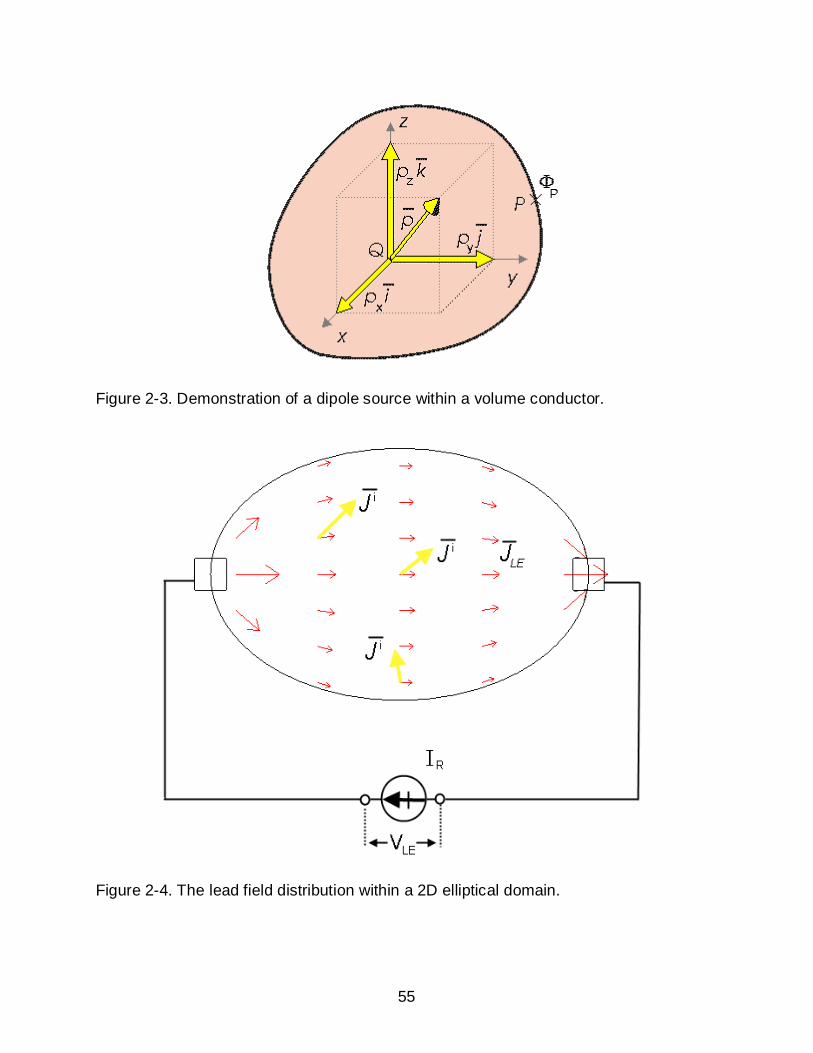
55
Figure 2-3. Demonstration of a dipole source within a volume conductor.
Figure 2-4. The lead field distribution within a 2D elliptical domain.

56
Figure 2-5. Illustration of the reciprocity theorem of Helmholtz
Figure 2-6. Derivation of the equation for lead field theory.
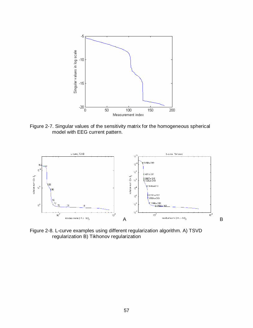
57
Figure 2-7. Singular values of the sensitivity matrix for the homogeneous spherical model with EEG current pattern.
A B
Figure 2-8. L-curve examples using different regularization algorithm. A) TSVD regularization B) Tikhonov regularization
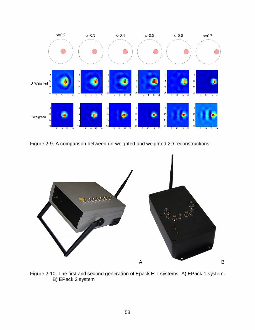
58
Figure 2-9. A comparison between un-weighted and weighted 2D reconstructions.
A B
Figure 2-10. The first and second generation of Epack EIT systems. A) EPack 1 system. B) EPack 2 system

59
Figure 2-11. Comparison of aperture times in EPack1 and EPack2.
Handheld
Computer
(Windows CE)
E-pack
E-pack
module
Flexible Connector
Radio
Communication
Flexible Electrode Belt
Figure 2-12. Overall system design of the EPack1 system
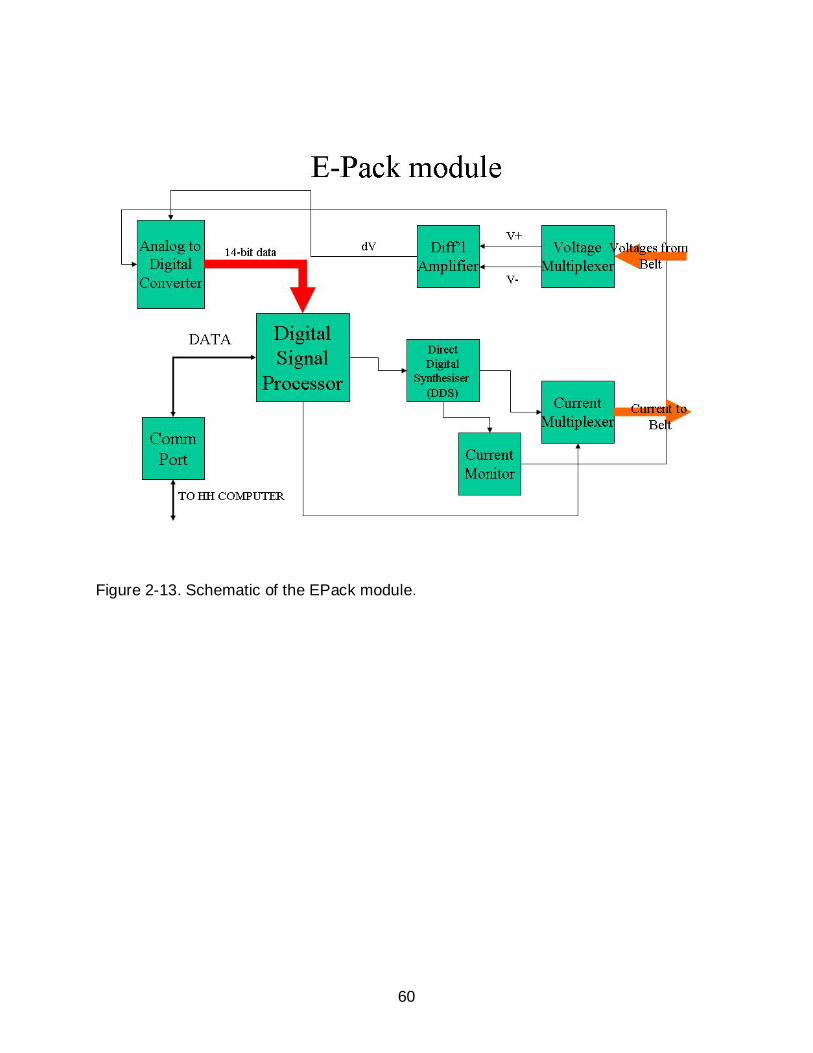
60
Figure 2-13. Schematic of the EPack module.

61
Figure 2-14. The EPack module, showing battery pack (top right), main acquisition board (center) and electrode connections (center)

62
Figure 2-15. EPack software screenshot (left). Amplified reconstructed image (top right). Phantom experiment using a full-array electrode configuration (bottom right).

63
CHAPTER 3 PIGLET SKULL IMPEDANCE MEASUREMENT
Background and Significance
Measuring dielectric properties of human tissues has been of research interest
since the 19th century (Epstein and Foster 1983). Knowledge of electrical properties of
human tissues is important for researchers to model different parts of human body
mathematically and investigate electrical related phenomenon. For example, it is well
known that the EEG source localization problem (EEG inverse problem) is highly
dependent on the knowledge of electrical resistivities of the tissues in the head
(Pohlmeier et al. 1997, Awada et al. 1998). It is also well established in EIT inverse
problems that incorrect skull conductivity information will bring in localization errors
when reconstructing conductivity changes within the head (Ni et al. 2006, Tidswell et al.
2001c).
The conductivity of the adult human skull was reported to be 0.015 S/m by
Oostendorp et al. (2000). To date, little data has been reported on the conductivity for
neonatal skulls. A neonatal skull differs from an adult skull in significant ways. The
neonatal skull is much thinner than the adult skull. In addition to that, it has an open
fontanel on top, which will finally fuse up as the skull develops. Sadleir and Argibay
(2006) reported that the conductivity of a neonatal piglet skull was 0.06 S/m, which was
about 4 times more conductive than the adult human skull. In this study, we measured
the radial conductivity of piglet skulls at different frequencies using an Electrical
Impedance Spectroscopy technique. We aim to find a relationship between skull
conductivity, skull thickness and piglet age.

64
Method
Sample Preparation
Skull bone samples were extracted from nine piglet skulls. Conductivity
measurements were performed on seven of the piglet skull samples as soon as
possible after piglets were euthanized. For the other two piglet samples, the
measurements were performed after the skull samples were frozen. The intact skull was
removed using a bone saw. The skull bones were when separated along suture lines
into right and left parietal and frontal bones (Figure 3-1).
Measurement Apparatus
The impedance data was collected using a Bio-impedance Spectroscope (BIS)
device developed by the EIT group at Kyung-Hee University, Korea. Using this device,
impedance can be measured within a frequency spectrum ranging from 10 Hz to 500
kHz.
To measure the radial conductivity of the skull, we constructed a measurement cell
similar to the one used by Oostendorp et al. (2000). The cell (Figure 3-2) was designed
for a four-terminal measurement strategy. It consisted of two cylindrical containers.
Each container had one end sealed and the other end open. A rubber O-ring was
attached at both open ends. When measuring skull conductivities, we filled the two
cylinders with saline, and put the skull sample between the two rubber rings. We then
sealed the two parts together tightly with 4 screws on the corners. Current was applied
through the two sealed end, and voltage was measured on the two voltage electrodes in
between. There was another electrode between the two voltage electrodes, used for
grounding the BIS current source. The diameters of the O-rings were 10.16 mm (0.4

65
inches). The distance between the two current electrodes was about 6.5 cm. The
distance between the two voltage electrodes was about 4 cm.
All the conductivity measurements reported in this thesis were carried out at the
frequency of 1 kHz, since this frequency was best calibrated. A total of ten data sets
were collected and then averaged for each skull sample. All the measurements were
taken at an ambient room temperature of 22 C° .
Theory
Skull resistivity values were calculated using equation 3-1. Conductivity is
calculated by taking the reciprocal of the resistivity (equation 3-2).
ARl
ρ = (3-1)
1σρ
= (3-2)
In equation 3-1, A is the cross-sectional area of the O-ring, which can be
calculated from its diameter. l is the thickness of the skull sample. Generally, the skull
samples were not uniform in thickness. Therefore, for each sample we measured the
thickness at three points on the edge using a caliper, and then took the average value.
R is the impedance of the skull sample. This impedance can not be measured directly.
We first determine the impedance of saline ( salineR ) by filling up the cell without tissue
between the O-rings. We then measured the impedance with the skull in place. The
value measured here was the serial impedance for the saline and the skull sample
( saline skullR + ). Therefore, the skull impedance R can be calculated as saline skull salineR R+ − .

66
Result
Table 3-1 lists the thicknesses and radial conductivities calculated for skulls
samples from 5 fresh piglet heads. All the piglets were no more than 3 days old. The
measurements were all performed within 5 hours after the animals were killed.
Measurements were also taken on skull samples obtained from a frozen piglet head.
The thickness and conductivity values for these samples are shown in Table 3-2.
The mean value of the radial conductivities was found to be about 27.8 mS/m with a
standard deviation of 11.8 mS/m. A plot of the measured values of radial conductivity as
a function of skull thickness is shown in Figure 3-3. The results obtained with both the
fresh samples and the frozen samples are shown with error bars. We calculated relative
errors as in equation 3-3, where Aε , lε and Rε denote relative errors in the
measurements of area, thickness and impedance. Aε was calculated to be around 12%,
and Rε was always around 5%. Because the thickness was a small number, the error
was mostly introduced by lε which can be as high as 30%. The solid line represents the
best fit to the data taken with fresh samples using a linear regression approach. The
equation of the best fit is also indicated near the line in the figure. The slope of the line
is about 21.58 mS/m2. The value of the linear regression (R2) was 0.467.
( ) A l Rε σ ε ε ε= + + (3-3)
Discussion
We report radial conductivity values in piglet skulls much higher than those
reported by Oostendorp et al. (2000) and Akhtari et al. (2002) in fresh or live adult skull.
The average value of radial conductivity obtained in the present study is 27.8 mS/m.
Using an apparatus similar to the one used in this study (Figure 3-2), Oostendorp et al.

67
(2000) reported the conductivity of fresh and live adult skull to be 15 ±3 mS/m. Akhtari
et al. (2002) have found the value of radial conductivity to be 9.53 ± 0.29 mS/m in live
skull. Our value is 40% and 60% higher than those obtained by Oostendorp et al. (2000)
and Akhtari et al. (2002) respectively. Thus our study shows that the conductivity of
neonatal skull is higher than adult skull. We also report a linear increase in the
conductivity with the increase in thickness of the neonatal skull. The reason for this is
suspected to be the cancellous bone in a thicker skull. No previous study exists that
explores the relationship between the conductivity and the thickness of the neonatal
skull.
All the measurements in this study were performed on post mortem piglet tissue.
Goncalves et al. (2003) pointed out several problems in using animal tissue samples.
Firstly, it is known that death of the tissue induces changes in its electrical properties.
On the other hand, the resistivity of the tissues depends on factors such as the water
content, which might generate a change resistivity during the measurement.
Physiological processes may also induce changes in the electrical properties of tissues.
Therefore, more research needs to be done to estimate the true in vivo electrical
resistivity of neonatal skull.
The calculation of skull resistivity also needs discussion. We used the O-ring area
for calculations using equation 3-1. The surface areas of the skull samples were all
larger than the O-ring area. When doing the measurements, current would flow beyond
the O-ring region and therefore make the equivalent cross-sectional area larger. This
effect may be neglected when the surface area is much larger than the thickness. A 3D

68
modeling study can be conducted to evaluate how much the result will be affected by
the equivalent area.
Conclusion
Measurements on neonatal piglet skulls show that the mean value of radial
conductivity is around 27.8 mS/m at a temperature of 22 C° and a frequency of 1 kHz.
This value is about 40% to 60% higher than that reported for adult skull. Moreover, our
measurements show for the first time that the conductivity increases as a function of the
skull thickness.
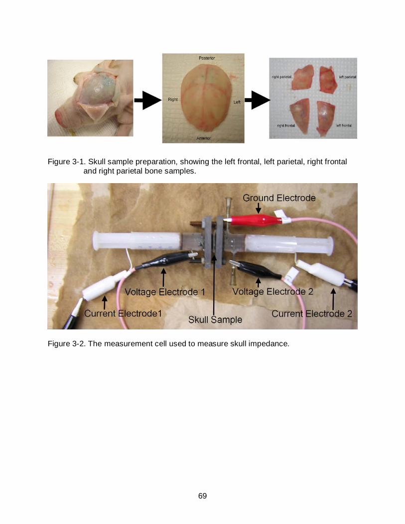
69
Figure 3-1. Skull sample preparation, showing the left frontal, left parietal, right frontal and right parietal bone samples.
Figure 3-2. The measurement cell used to measure skull impedance.

70
Table 3-1. Measurement results for the fresh skull samples.
Age
(days) Part
Thickness (mm)
Conductivity (mS/m)
Piglet I 2
Left Frontal 0.762 10.807 Left Parietal 0.720 6.898 Right Frontal 0.974 15.015 Right Parietal 0.593 5.940
Piglet II 3
Left Frontal 1.058 27.516 Left Parietal 0.931 18.033 Right Frontal 1.016 31.223 Right Parietal 1.185 22.019
Piglet III 2
Left Frontal 1.778 22.112 Left Parietal 1.270 19.241 Right Frontal 1.693 33.784 Right Parietal 1.101 14.889
Piglet IV 2
Left Frontal 1.609 43.957 Left Parietal 1.524 31.194 Right Frontal 1.609 41.935 Right Parietal 1.693 39.375
Piglet V 2
Left Frontal 1.609 43.956 Left Parietal 1.524 31.194 Right Frontal 1.609 41.935 Right Parietal 1.693 39.375
Piglet VI 1
Left Frontal 1.600 25.131 Left Parietal 1.350 21.910 Right Frontal 1.743 32.837 Right Parietal 1.133 14.511
Piglet VII 1
Left Frontal 1.433 39.432 Left Parietal 0.883 38.571 Right Frontal 1.300 41.954 Right Parietal 0.683 22.589
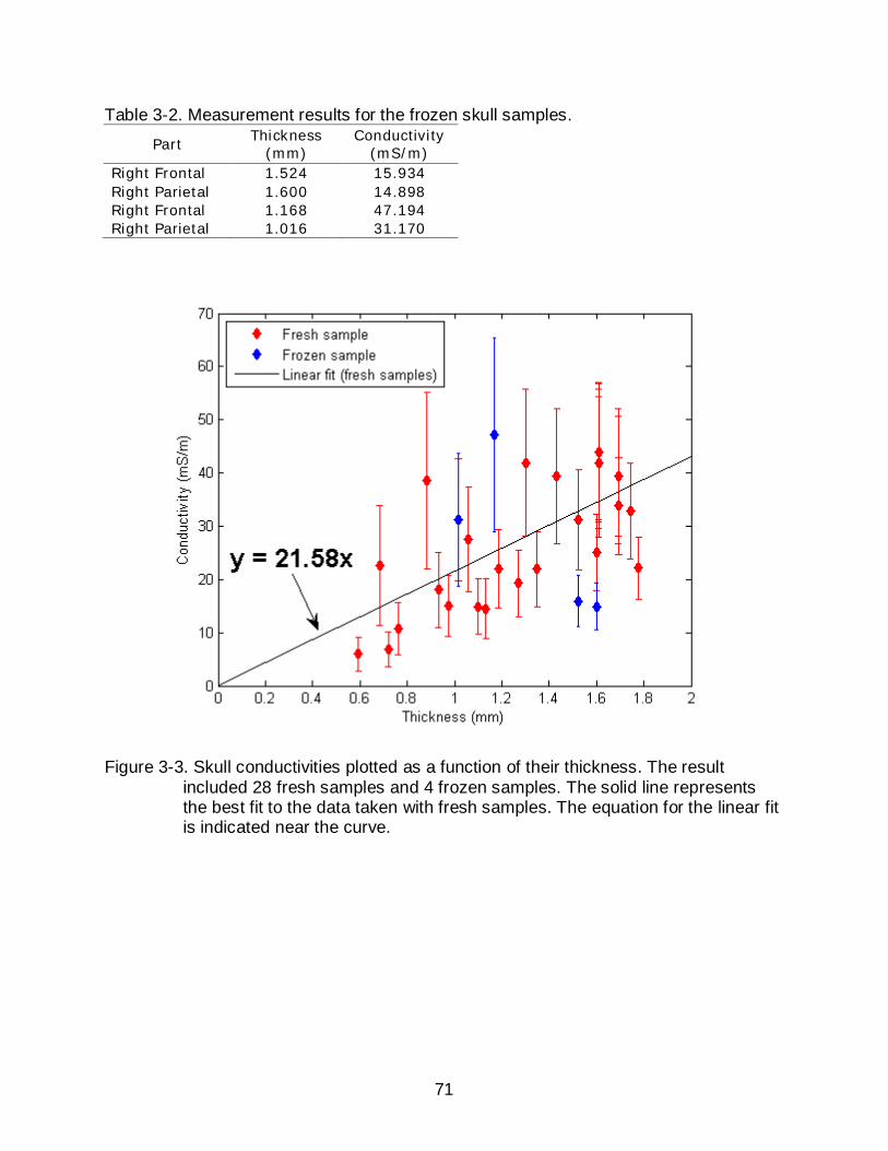
71
Table 3-2. Measurement results for the frozen skull samples.
Part Thickness
(mm) Conductivity
(mS/m) Right Frontal 1.524 15.934 Right Parietal 1.600 14.898 Right Frontal 1.168 47.194 Right Parietal 1.016 31.170
Figure 3-3. Skull conductivities plotted as a function of their thickness. The result included 28 fresh samples and 4 frozen samples. The solid line represents the best fit to the data taken with fresh samples. The equation for the linear fit is indicated near the curve.

72
CHAPTER 4 A ROBUST CURRENT PATTERN FOR THE DETECTION OF IVH
Background
Different electrode configurations and measurement strategies may be more
effective for different EIT applications. The classic RING electrode configuration has
been widely adopted in the EIT literature. The measurement strategies employed using
the RING electrode layout can be classified into the following categories: the
neighboring method (Brown and Segar 1987), the cross method (Hua et al. 1987), the
opposite method (Hua et al. 1987, Bayford et al. 1996) and the adaptive method (Gisser
et al. 1987, Zhu et al. 1993). There have also been studies and algorithms on optimizing
current patterns (Gisser et al. 1987, Koksal and Eyuboglu 1995, Lionheart et al. 2001).
However, an ‘optimum’ injection pattern may not always be the correct choice, because
minimizing the error on each channel would increase the hardware complexity (Bayford
2006). Other electrode configurations include using planar electrode arrays for the
detection of breast cancer (Kao et al. 2006), using a 2-plane electrode configuration for
lung imaging (Graham and Adler 2007), and using a hemi-array electrode configuration
for the detection of intraperitoneal bleeding (Sadleir et al. 2008a, 2008b, 2008c).
In this study, we performed simulations and phantom experiments, aiming to find
an effective current pattern for the detection of intraventricular bleeding in premature
neonates.
Method
Candidate Current Patterns
We investigated three 16-electrode layout strategies and current patterns. The first
one was a RING layout (Figure 4-1 A), where the 16 electrodes were placed equally

73
spaced in a single plane about the equator of the sphere. An ‘adjacent’ current pattern
was applied to this layout, that is, current was applied to a pair of adjacent electrodes
and resulting voltages across other pairs of adjacent electrodes were measured. The
second one was a standard EEG layout, following the 10-20 system of electrode
placement (Figure 4-1 B). Locations of EEG electrodes in spherical coordinates are
shown in table 4-1. The current pattern applied to the EEG layout was denoted ‘EEG’
pattern, and in this strategy currents applied were returned via an electrode on the apex
of the head, and voltages between adjacent electrodes (in terms of electrode
numbering) were measured. The EEG pattern therefore involved 15 current positions
and a total of 182 voltage measurements. The basis for formulating the ‘EEG’ current
pattern was the geometry of the infant human skull. Neonates have a fontanel located at
the top of the skull. We expect that when currents flow via an electrode situated over the
fontanel, there should be greater sensitivities to centrally located conductivity changes
compared to cases where the skull forms a complete barrier. Therefore, we chose to
test if the EEG current pattern may be useful to locate bleeding in neonates. The third
electrode layout we investigated was a ‘Cz-RING’ layout where one electrode was
located at Cz, and the other 15 electrodes were placed equidistantly about the equator
of the sphere (Figure 4-1 C). The current pattern applied in the Cz-RING case involved
all currents returning via the top electrode, and with all possible adjacent measurements
made on the 15-electrode ring. The Cz-RING pattern is thus a modification of the RING
pattern. The electrode at Cz should lead to increased sensitivities above the equator
plane. At the same time this pattern preserves the symmetry of the RING pattern. A

74
symmetric distribution may have an advantage in making post compensation of
quantification and localization errors easier.
To formulate sensitivity matrices, we constructed spherical head models (Figure 4-
2) with a unit radius and homogeneous conductivity distributions for each 16-electrode
layout using finite element modeling (Comsol, Burlington MA, USA). After creating
tetrahedral meshes, we solved these forward models for each current pattern and
calculated the sensitivity value corresponding to each mesh element. We constructed
26 126, 21 896 and 51 524 tetrahedral element models for the forward models with
RING, EEG, and Cz-RING electrode configurations respectively.
Sensitivity Studies for the Candidate Current Patterns
Inspection of anatomical MRI scans of the neonatal head indicate that the
ventricles are centrally located and if translated to a spherical geometry would lie in the
upper hemisphere at an elevation of around 0.3-0.5 of the sphere radius into the upper
hemisphere, as shown in Figure 4-3. Therefore we chose to study the sensitivities and
contributions total measured resistances in both regions on the central axis and in
regions having the same approximate size and location of the neonatal ventricles. The
sensitivity of a particular measurement is defined by equation 2-28. Thus, the
contribution of a particular region j to the thi impedance can be calculated by including
the conductivity of the region (equation 4-1).
( ) ( )j
j jij j jV
Z dvI Iφ ψ
φ σ ψ σσ
∇ ∇= −∫ (4-1)
The two central regions were spheres with relative radii of 0.25 compared to the
background sphere radius and were centered at z = 0.33 and z = 0.50. We refer to the
sphere at z = 0.50 as the upper sphere and the other as the lower sphere. The two

75
lateral ventricles, approximated as ellipses, were located in relative radial terms at (-0.2,
0, 0.3) and (0.2, 0, 0.3) each having semiaxis lengths of 0.15, 0.44 and 0.15 in x, y and
z axes, respectively. The four regions are illustrated in Figure 4-3. The spherical regions
(about twice as large as the ventricles) were chosen to compare with the lateral
ventricle region properties and to determine the uniformity of each pattern.
A useful current pattern should produce both a large sensitivity and selectivity in
the region of interest, and produce a consistent response in the neighborhood of the
region of interest.
To evaluate the three candidate current patterns, we compared the sensitivities,
selectivities and maximum and half sensitivity volumes of the current patterns within
both central and lateral ventricular regions. Sensitivity values were expressed as the
mean sensitivity over the region of interest as a fraction of the maximum sensitivity over
the entire domain, for each measurement configuration in the scheme. The selectivity
(Kauppinen et al. 2005, Yang and Patterson 2008) is the fraction of the total measured
resistence contributed by the central region, and the half and negative sensitivity
volumes measured over the sphere. The half sensitivity volume is defined as being the
volume of the sphere that has more than half the maximum sensitivity for a particular
pattern. The negative sensitivity volume is the volume of a particular measurement
pattern occupied with negative sensitivity, i.e. the volume of elements that produce
contributions to the total measured resistance in an opposite direction from that
expected. In most four electrode measurement schemes there will be significant
negative sensitivity regions (Kauppinen et al. 2005, Yang and Patterson 2008). In
principle, negative sensitivity is not bad. If an appropriate model is used, it should be

76
possible to relate any observed change to the correct sign of conductivity change.
However, negative and positive sensitivities will sum to form the total measured
resistance, and it is possible that for some current patterns location of negative
sensitivities may be a problem and produce contradictory information. This could occur
if, for example, there is a mismatch between model and experimental conditions. The
half sensitivity volume gives an indication of the breadth of the positive sensitivity
distribution.
Data Generation
We gathered simulated bleeding data using finite element models and saline-filled
phantoms.
Finite element models
To obtain more realistic boundary measurements and evaluate the effects of other
head structures on reconstructions, we constructed two finite element models to mimic
electrically important structures in the infant skull. In order to compare the various
current patterns fairly, we tested each pattern (RING, EEG and Cz-RING) using data
gathered using the same bleeding layout structure (Figure 4-4). This structure (the A
model) included a central region of CSF, having a relative radius of 0.5, and an outer
shell of grey & white matter. We simulated a small amount of bleeding inside this model
by placing a small sphere of blood with a relative radius of 0.05 at 37 different locations
within a central bolus of CSF. The volume of the CSF region in model A is much larger
than the realistic ventricle size. However, using a large CSF background produces a
smaller relative change in the overall measured transimpedances than with realistically
sized ventricles. This model was adopted as a first step because we were interested to
see the overall performance of each current pattern under this more stringent condition.

77
Comparisons between different current patterns were made in reconstructed images in
terms of anomaly localization, reconstruction quality and quantification stability. We also
made a more complicated model, used with the EEG current pattern and RING current
pattern only. In this model (the B model), we changed the CSF geometry from spherical
into two small elliptical spheroids, to simulate the two lateral ventricles. The simulated
ventricles were placed in the upper hemisphere. The size and position of the ventricles
were chosen from representative neonatal head MRI data (Figure 4-6) (Schierlitz et al.
2001). We determined that the total lateral ventricle volume was about 1/70 of the head
volume. The minor and major axis of each ellipse was chosen to be 0.3 and 0.88 of the
sphere radius respectively. A blood-like anomaly with a relative radius of 0.1 was moved
to 6 different locations within the ventricle regions (Figure 4-5). In addition to the CSF
geometry change, we also introduced a skull shell with a fontanel on top, another thin
layer of CSF between the brain and skull, and a scalp layer outside the skull. The
conductivity of each structure was assigned according to values from the literature. The
values used were: blood (0.67 S/m) (Geddes and Baker 1967), CSF (1.3 S/m)
(Oostendorp et al. 2000), brain (0.17 S/m) (Stoy et al. 1982), and scalp (0.43 S/m)
(Burger and van Milaan 1943). The conductivity of the neonatal skull was assigned to
0.06 S/m (4 times of that of the adult skull) according to preliminary data obtained using
piglet skull (Sadleir and Argibay 2006)
Phantom models
Phantom experiments were conducted to allow testing of how each current
pattern, electrode layout and reconstruction performed in the presence of realistic noise.
Our spherical phantoms used only the RING and EEG layouts respectively (Figure 4-7).

78
The spherical polycarbonate containers were obtained from a manufacture of lighting
fixtures (Formed Plastics, NY, USA). Each phantom was equipped with 16 stainless
steel electrodes (dia. 14 mm) according to their electrode configuration. Both phantoms
had inner diameters of 19.7 cm.
We used 0.6% saline solution (the conductivity of which was approximately 1.3
S/m, the conductivity of CSF (Oostendorp et al. 2000)) as the phantom background and
gel anomalies made using TX151 powder (Walker et al. 2004). TX151 is a solidifying
medium that produces a stable gel-like material when mixed with water, agar and
saline. By carefully adjusting the percentage of each ingredient (Deionized water 80.8%,
Sucrose 13.8%, Agar 2.5%, TX151 2.5% and Sodium chloride 1.3%), we made the
anomaly conductivities approximately 0.67 S/m (the conductivity of blood). Further
details of anomaly construction may be found in Sadleir et al. 2009. Anomalies had
diameters of 2cm (a relative radius of 0.1). The size ratio between the phantom and the
anomaly was therefore approximately the same as those used in simulations on model
B. A single anomaly was placed accurately at the same 6 positions used in model B
(Figure 4-5), using the 3D Positioner (Velmex Inc., NY, USA).
Data was collected with a 16-electrode EIT system provided by Impedance
Imaging Research Center at Kyung Hee University, Korea. This is a multi-frequency EIT
system with a frequency range from 10 Hz to 500 kHz (Oh et al. 2007). We chose to
use a single frequency of 10 kHz and a constant current output of 1 mA. This frequency
was chosen because the impedance properties of both TX-151 and saline are flat over
the interval 10 Hz – 50 kHz (Sadleir et al. 2009) and 10 kHz was well calibrated in the
center of this range. The reference electrode for the system was a copper wire placed at

79
the center of the phantom ‘neck’. Ten data sets were collected before anomalies were
introduced. These were averaged and used as the reference data set. For each
anomaly position, five data sets were collected and averaged as the perturbation data
for that anomaly position. The overall experiment system is shown in Figure 4-8.
Reconstruction Method
All the time-difference images in this study were reconstructed from the boundary
measurements using a one-step sensitivity based method (equation 4-2), which has
been discussed in detail in chapter 2.
†S Vσ∆ = ∆ (4-2)
In EIT, the sensitivity matrix is always severely ill-conditioned and will therefore
have large condition numbers. Each of the three sensitivity matrices used in this study
had a full rank of 104 but involved a measurement strategy that involved making a
larger number of observations, as shown in table 4-2. Typical condition numbers were
of the order of 1910 for the RING strategy, 1410 for the EEG strategy and 1210 for the Cz-
RING strategy. The inversions of the sensitivity matrices were regularized using the
TSVD method. The truncation point, k , will be less than or equal to the rank of the
matrix, but in general will be less depending on the noise level in the voltage
measurements. We chose k values for our reconstructions by inspecting images
generated using a range of truncation points and determining the maximum value that
produced a coherent reconstructed image. The truncation values needed to be chose
carefully since inappropriate truncation values would produce inaccurate solutions. The
optimal truncation numbers for the problems in this study are between 50 and 70, and
were evaluated with the l-curved method. The bottom row of table 4-2 lists the

80
truncation points we chose for each case using this heuristic method. Truncation points
of 60 and 50 were used for simulated and experimental cases respectively.
Localization of EIT Reconstructions
The location of conductivity changes can be estimated from reconstructed images.
The location of a single perturbation can be determined by equation 4-3. The
expression for anomaly location (x, y, z) is effectively the ‘center of mass’ of the
difference image. The values , ,i i ix y z are the coordinates of the center of each element.
iσ∆ is the conductivity change reconstructed in the ith element and v is the volume of
each element.
1 1 1
1 1 1
, ,
ne ne ne
i i i i i i i i ii i i
ne ne ne
i i i i i ii i i
v x v y v zx y z
v v v
σ σ σ
σ σ σ
= = =
= = =
∆ ∆ ∆= = =
∆ ∆ ∆
∑ ∑ ∑
∑ ∑ ∑ (4-3)
Errors in reconstructed locations were calculated as the absolute location errors
quoted as a fraction of the model or phantom radius (‘relative radial error’). We
considered separately horizontal errors (errors within the xy plane) and axial errors
(errors in z direction) respectively for each of the three current patterns. Therefore, we
define these values as:
Dxy = ∆x( )2 + ∆y( )2 R (4-4)
zD z R= ∆ (4-5)
Image Resolution and Contrast
We compared image resolution using a method based on one suggested in Adler
et al. (2009), wherein we estimated the relative volume contained in the set of voxel
anomalies that had reconstructed values more than half the maximum within the image

81
0
HMVV , where 0V is the entire model volume, and then took the cube root of this value.
That is, for each image we computed the value
3
0
HMVRV
= (4-6)
The half maximum threshold was also used to construct isosurfaces for display of
reconstructed anomalies. Use of this measure allowed comparison of both the extent of
artifacts within images (as large artifacts will tend to increase the apparent resolution)
and the true resolution in ventricular regions. We examined the ability of our
reconstruction to resolve two anomalies by examining the reconstructed profile through
a line joining the two anomalies. We defined the two anomalies as resolvable if the
value between the anomalies reached a value half the maximum conductivity found on
the profile.
We compared image contrast c for different reconstructions by first finding the
average image value over a region having the same size as the original anomaly that
was placed in the lower hemisphere ( Bc ), far away from artifacts and the anomaly
reconstruction. We then took the difference between this value and the average
conductivity in the region of the reconstructed anomaly, centered on the maximum
reconstructed voxel value ( Mc ). Thus we have the definition of image contrast (equation
4-7). Larger contrast values corresponded to better reconstruction qualities.
M Bc c c= − (4-7)

82
Comparison between ‘Open Skull’ and ‘Closed Skull’ Models
Sensitivity analysis using a layered model
The effects of outer head composition may be significant (Gibson et al. 2000). We
therefore evaluated the sensitivity performance of the EEG-based pattern using a partial
prior spherical model that incorporated layers of skin, skull (with and without the
fontanel) and CSF, the center of the head being assigned to have the same conductivity
as brain. Layer thicknesses were chosen according to data gathered from inspection of
archived neonatal MRI models. The diameter of the model was chosen to be 11.9 cm (a
volume of 884 ml), with a scalp thickness of 2.9 mm, skull thickness of 6.0 mm and CSF
layer thickness of 3.0 mm. The archived MRI data set used as a reference had a total
volume of 921 ml. A 41626 element (62118 nodes) tetrahedral finite element model was
created using the layer scalings noted above. The model outline is shown in Figure 4-9.
Regions were assigned conductivities found in the literature: scalp (0.43 S/m, Burger
and van Milaan 1943); CSF (1.3 S/m, Oostendorp et al. 2000); brain tissue (0.172 S/m,
Stoy et al. 1982). We chose the skull conductivity to be either that of adult skull (15
mS/m, Oostendorp 2000) or piglet skull (60 mS/m, Sadleir and Argibay 2006). We
chose to use the conductivity for neonatal piglet skull in the absence of values for
human neonatal skull in the literature, and because the neonatal piglet will be used as
an animal model in future tests of this technique. The layered model was tested with the
EEG layout only. In order to determine the interaction between the presence of the
fontanel and the EEG measurement layout, the part of the head designated as fontanel
in Figure 4-9 was either chosen to have the conductivity of skull or skin, corresponding
to either ‘closed’ or ‘open’ skull conditions respectively. Sensitivity matrices were
calculated for each of these configurations. We found the condition numbers for closed

83
skull cases were generally lower than for open skulls, with values for adult skull
configurations being about 158.8 10× and
161.6 10× , respectively; and for piglet skulls
153.5 10× and 154.2 10× .
Noise analysis using model B
The spherical model shown in Figure 4-9 represents an ‘open skull’ model, since
we assigned the scalp conductivity (0.43 S/m) to the fontanel. We constructed another
‘closed skull’ model by setting the fontanel conductivity to be the same as the skull
conductivity (0.06 S/m). In this study, we compared the performance of the EEG current
pattern on both open and closed models by comparing the reconstructed images when
different levels of white Gaussian noise were introduced to the measurements. The
noise levels were determined by the SNR levels of practical EIT systems. The KHU
Mark1 system was reported to have an average 80-90 dB for SNR (Oh et al. 2007). An
SNR of 50-60 dB was observed with simple phantom experiments using the ITS P1000
system (Murrieta-Lee et al. 2004). Therefore, we made comparisons with 50dB, 65dB
and 75dB introduced Gaussian noise. We added noise to the model data by first
measuring the signal power, and then adding noise at the specified SNR level using the
MATLAB function ‘AWGN’. Noise was added first to the reference data and then to data
from a case with an anomaly present. These two sets were subtracted from each other
to form the voltage perturbation. For each noise level and skull composition, we created
100 data sets. We compared the resulting resolution and contrast values in the
reconstructed images at the same noise level for the two skull conditions a priori using t-
tests.

84
Results
Sensitivity and Selectivity for the Uniform Models
Sensitivities to bleeding in the central part of the head were investigated by
computing sensitivities in the regions of interest. This is similar to the approach used by
Kauppinen et al. (2005) where sensitivities in the center of a disk were compared using
different measurement configurations. Sensitivity maps for the four regions of interest
are show in Figure 4-10 for all three patterns on the uniform sphere. For a significant
number of measurements sensitivity was negative. The RING pattern had the most
positive sensitivity values. The average sensitivity of the EEG pattern was greater than
either RING or Cz-RING patterns for the upper sphere, and comparable to the RING
pattern over the lower sphere. However, the EEG pattern had significant regions of
negative sensitivity. On the basis of sensitivity alone, the RING pattern was superior to
Cz-RING and EEG patterns, as it demonstrated mostly positive values in the regions of
interest. The Cz-RING pattern had reasonable amplitude sensitivities but demonstrated
an average negative sensitivity for both regions of interest. Examination of Figure 4-10
C and D shows that in the ventricles EEG pattern sensitivities were similar to those in
the lower sphere and that there were significant negative sensitivities. The RING pattern
sensitivity peaks were much larger than the EEG pattern peaks for both ventricle
samples. The Cz-RING pattern plots for simulated ventricles shifted considerably
compared to the spherical region results and there are many large negative sensitivity
values.
Where as the sensitivity of the models reflects the interaction between current and
measurement pair geometries in the model, the selectivity shows the contribution from
the target region to measured voltages and transimpedances. Absolute selectivities for

85
the uniform spherical pattern were clearly better than either Cz-RING or RING layouts,
with up to 15% of total resistance contributed by the upper sphere and 7-10% of total
resistance typically contributed by the lower sphere (Figure 4-11). EEG pattern
selectivities in the ventricles were slightly smaller than those observed in the lower
sphere, with average values being around 4%, but these values were on average larger
than those observed for the RING pattern. Selectivities for the Cz-RING pattern in the
ventricles were also relatively high, averaging about 3% with peaks up to 6% of total
resistances.
Negative sensitivity volumes for all spherical background models were large,
averaging around 50%. The negative sensitivity volumes of the three patterns were
around 70%, 35% and 53% for RING, Cz-RING and EEG patterns, respectively. By
contrast, half-sensitivity volumes were usually very small, being about 0.6% for the
RING, 0.3% for Cz-RING and 0.2% for the EEG pattern. The results broadly agree with
sensitivity analyses performed using four electrode configurations in 2D (Kauppinen et
al. 2005) and in 3D (Yang and Patterson 2008).
Comparing the Three Current Patterns Using Model A
The performances of the three current patterns on model A were compared in
terms of localization errors and QI stabilities. Figure 4-12 A compares xyD for the three
current patterns and Figure 4-12 B compares zD for the EEG and Cz-RING patterns
only, since the RING pattern was not able to localize in the z direction. The
quantification stabilities of the three current patterns are compared in Figure 4-13. In
order to compare the quantification stability between different current patterns, the 37
QIs were normalized with respect to their average for each current pattern. The EEG

86
current pattern showed the best performance for anomaly positions above the equator
in terms of both localization errors and quantification stability. The RING current pattern
could localize anomalies very well in the xy plane, and showed a great potential in
overall quantification stability. The Cz-RING current pattern could determine the axial
position for the anomalies above the equator and off the central axis, but performed
very poor for the anomalies on the central axis. Its overall performance was only slightly
better than the ring pattern alone.
Comparing RING and EEG Patterns Using Model B and Phantom Data
We compared the performance of the RING and EEG current patterns on model B.
Cz-RING was not used for phantom measurements due to its poor performance on
model A. Results for reconstructions of simulated and phantom data using both current
patterns and sensitivity matrices are shown in Figure 4-14. Figure 4-14 (a) shows an
ideal image of bleeding accumulation at position 1, a relative radial position of (-0.2,
0.25, 0.3), illustrated in axial and sagittal sections and as isosurfaces, with results for
reconstructions of (b) simulated EEG data, (c) simulated RING data, (d) phantom EEG
data and (e) phantom RING data. Isosurfaces were calculated at a threshold set at half
the maximum voxel value within the image. As expected, the RING pattern could not
determine axial positions of anomalies because of its two dimensional symmetry.
Resolutions in reconstructions from all phantom data appeared similar to
reconstructions from simulated data, but contained artifacts, as reflected in results
shown in Table 4-3. In most cases, the characteristic size of reconstructions for EEG
cases was smaller than those for the RING cases. Interestingly, although it is clear that
in both comparisons of anomaly 1 reconstructions that those for the RING were more

87
diffuse, the R measure gave a smaller value for RING resolutions than for EEG
resolutions.
The EEG pattern could localize well in all three dimensions. Figure 4-15 shows
that the RING pattern localized anomalies as well as the EEG pattern in the xy-plane,
producing a maximum radial relative error of 0.035 in both cases. The EEG pattern
localized the z-coordinate well in simulated data, with the maximum Dz less than 0.03 of
the radius over all intraventricular locations. Localization errors were larger for
reconstructions from both current patterns applied to the phantom case, with the worst
value of Dxy being 0.17 for the EEG pattern and 0.1 for the RING pattern.
The QI values found were comparable to the ideal QI, which can be calculated as:
3 24( ) ( ) 0.0026 [ ]3ideal blood CSF bloodQI r Smσ σ π= − = − (4-8)
Quantification results for the RING pattern were similar to those for the EEG
pattern for simulated data, with the largest variation no more than 5% for both cases.
Quantification results from phantom data were also similar, although QI errors found
using the RING pattern were very large in some cases. The worst QI error in
reconstructions using the EEG pattern with phantom data was around 10% while the
worst QI error in corresponding RING pattern phantom reconstructions was almost 30%
(Figure 4-16).
Comparison between ‘Open Skull’ and ‘Closed Skull’ Models
Comparisons of reconstructions of a blood-like anomaly at position 1 using the
EEG current pattern with open and closed skull models are shown in Figure 4-17. The
advantage of using a fontanel-focused pattern was made visible when 50 or 65 dB
Gaussian white noise was added to data. At 50 dB the open skull model had resolution

88
0.1805 and contrast 0.5228, while the closed skull model had a resolution of 0.1959 and
contrast 0.5158. At 65 dB we could still locate a peak conductivity change at a location
corresponding to the anomaly position in an open skull reconstruction (resolution R =
0.187, contrast c = 0.523) while the reconstruction on the closed-skull model was almost
completely dominated by artifact (R = 0.205, c = 0.499). Both images were still affected
at 75dB noise levels, with open skull resolution and contrast being 0.222 and 0.473
respectively and closed skull resolution and contrast being 0.235 and 0.467
respectively. In the 50 and 65 dB cases, R and c values were significantly better
(p < .05) for open skull cases than for closed skull cases. At higher SNR levels (75 dB
and above) we found that resolutions and contrasts were not significantly different.
Discussion
Sensitivity and Selectivity
Sensitivity and selectivity parameters of the three different measurement
strategies can be used to predict their ability to detect changes in the ventricular
regions. A robust measurement method should have both high selectivity and high
sensitivity in the region of interest. We have found that the EEG measurement pattern
had similar magnitude sensitivity to the RING pattern in the two spherical regions of
interest, but higher selectivities. In addition, the EEG pattern had both maximum
measured transimpedances and a lower dynamic range than the RING pattern.
Although the RING pattern had a stable sensitivity distribution and good selectivity,
it can not be used to determine three-dimensional anomaly locations because of its
planar symmetry. The presence or absence of the fontanel, and skull conductivity
greatly affect sensitivity distributions. The Cz-RING pattern had lower sensitivities than
the RING pattern in all cases, with the average sensitivity being negative for both

89
regions of interest tested. Selectivities of the Cz-RING pattern were comparable to
those of the EEG pattern, but Cz-RING pattern’s overall negative and variable
sensitivity in central regions indicates it may be unsuitable for practical measurements.
Because of the symmetry of the EEG layout, there were several very low values
for resistance predicted (24 of the 182 used). In our analysis of selectivity, we chose to
ignore these data. We expect that broadly similar patterns to those obtained for
spherical model-based matrices would be found when testing the RING or Cz-RING
patterns on realistic geometries. For example, the negative and low sensitivity values
found for the Cz-RING method would also be anticipated in a realistic geometry model
as these are a consequence of measurement and current field patterns being
orthogonal or opposed in central regions for many measurements. While the EEG
pattern seems promising, it is possible that there are superior measurement strategies
that can be devised using the same layout, but avoiding measurement of near-zero
values. However, the number of independent measurements possible with this number
of electrodes (104) will always limit the available information.
Overall Evaluation with Model A
Simulation results from model A confirmed part of the findings from sensitivity
analysis. We found from the localization errors that the RING current pattern could
identify x and y positions well, with the worst error in xyD obtained for this current
pattern using simulated data being less than 0.08 of the sphere radius over all 37
locations. The EEG pattern could localize well in all three dimensions, especially for the
anomaly positions above the equator, with the worst error being 0.07 in the xy plane
and 0.09 in the z direction. The Cz-RING current pattern could localize in the z direction

90
for some cases above the equator, but not consistently. Comparing the simulation
results on model A in terms of QI stability, we found the EEG pattern showed a smaller
variation than the other two current patterns for the anomaly positions above the
equator, and therefore a better potential to quantify bleeding. The RING pattern showed
the smallest QI variation overall in the simulation results on model A. However, in the
problem of quantifying intraventricular bleeding, the EEG pattern seems a better choice
because we expect that the intraventricular bleeding will occur above the midplane of
the head.
The Cz-RING current pattern is supposed to combine the advantages of both the
RING pattern and EEG pattern. We used both coarse (22093 elements) and fine (51524
elements) sensitivity matrices to reconstruct Cz-RING data, but found that although
increasing the number of elements improved localization and QI results slightly, they
were still not significantly better than the RING pattern alone. The Cz-RING pattern did
improve localization in the z direction over the RING pattern, but not consistently. One
interesting finding from Cz-RING pattern data was that we could localize the z positions
when the anomaly was off the central z-axis, the more the better. However, when the
anomaly was close to or on the central z-axis, it performed only as well as the RING
pattern. This indicated that the Cz-RING pattern was not sensitive enough for the
location changes on the z-axis because the current stream lines generated by the drive
electrode pairs were almost perpendicular with the current stream lines generated by
measurement electrode pairs on the central axis.
Model B and Phantom Experiment Results
Again, both the RING and EEG patterns performed well in terms of xy-plane
localization and quantification accuracy on reconstructions of simulated data generated

91
from model B, with the localization results shown in Figure 4-15 confirming our
observations from the reconstructed images of Figure 4-14. Localization accuracy was
slightly worse for the phantom data, presumably because of the presence of random
and systematic experimental noise. We believe that the large localization errors for
positions 4, 5 and 6 in the EEG phantom experiment shown in Figure 4-15 may have
been caused by a degradation in anomaly quality after it had been immersed in the
saline background for some time (each set of measurements at a single anomaly
volume were performed by moving the anomaly around the tank over a period of
approximately 10 minutes (Sadleir et al. 1998, Sadleir et al. 2006)), but they may also
have been caused by the slight lateral asymmetry of the sensitivity matrix combined
with noise. As shown in Figure 4-16, the QI variability in the noiseless simulated data
was relatively flat in both cases, with the largest variations being no more than 5%. As
with localization performance, phantom results tended to agree with the simulation
results, but we observed larger QI variations for phantom cases. Figure 4-16 also shows
that the EEG pattern performed better than the RING pattern in phantom experiments,
confirming results of our sensitivity analysis. The sensitivity analysis of the two patterns
showed that the RING current pattern had a much lower selectivity than the EEG
pattern in ventricular regions. Therefore for the same conductivity perturbation, smaller
voltage changes were produced, as a consequence of which the noise played a more
significant role in the RING phantom measurements. On closer inspection of data
vectors, we found that the normed sum of the voltage perturbation caused by a single
blood-like anomaly within a ventricle was about 1/5000 that of the normed sum of all
reference measurements for the RING pattern, and about 1/1000 for the EEG pattern.

92
The SNR level of the KHU Mark1 system was reported to be 80-90 dB (Oh et al. 2007).
This implies that noise accounted for 17-50% of RING phantom data, while accounting
for only 3-10% of EEG phantom data. As a result, the QI values were more severely
contaminated by the noise-generated artifacts in reconstructions based on the RING
current pattern.
Anomaly Quantification
Absolute QI values do not only depend on the size of the anomaly, but also
depend on the current pattern’s sensitivity matrix and the truncation point used. For
example, the RING pattern and EEG pattern produced different sensitivities in the
ventricle regions, and therefore had different QI accuracy for the same anomaly
presented in this particular region. A truncation number of 50 was used for all the
phantom experiments in this study. A different truncation point would shift all the
absolute QI values to another level. In practice, we can determine the relationship
between QI and anomaly volume with an EIT system calibrated for a particular
configuration and truncation number using a phantom and blood-like anomalies (Sadleir
et al. 1998, Sadleir et al. 2008). Variations of up to 30% were observed in QI values for
anomalies moved within ventricular regions of the RING spherical phantom, and up to
10% using the EEG pattern and phantom, an observation that was correlated with poor
localization in the xy-plane. This may have been related to the overall smaller selectivity
found for RING pattern in ventricular regions, combined with measurement noise. Even
though the EEG pattern showed generally good results, some method of QI
regularization that reduces its shift variance may be appropriate. We have results of
implementing such a method in 2D 16-electrode reconstructions (Oh et al. 2009, Sadleir
et al. 2008). This algorithm gave very promising results in 2D, resulting in a reduction in

93
QI spatial variability to about half. The method may be straightforwardly extended to
3D. We believe that use of a similar approach with the EEG pattern would likewise
make QI accuracy greater in the present context.
Comparison between ‘Open Skull’ and ‘Closed Skull’ Models
We chose to compare the open skull and closed skull models using three different
levels of Gaussian noise (50 dB, 65 dB and 75dB), which were chosen from the range
of SNR values reported for practical EIT systems (Oh et al. 2007, Murrieta-Lee et al.
2004). Our sensitivity analysis showed that the EEG pattern has on average a 7-10%
larger selectivity near the ventricle region on the open skull model than on the closed
skull model (Sadleir and Tang 2009). This, in conjunction with the overall larger
sensitivities observed in open skull cases, indicates that perturbations inside the lateral
ventricle region should contribute larger relative voltage changes with an open skull
than with a closed skull. Therefore, the EEG pattern should have a greater potential to
detect and localize a perturbation within the ventricle regions when the fontanel-like
opening is included. The comparison of the reconstructed images in Figure 4-17
demonstrated that the EEG pattern produced overall better images on the open skull
model than on the closed skull model, especially at low SNR levels. The implication of
this is that the EEG pattern should produce superior images on neonatal skulls than
(closed) adult skulls. Images produced above 75dB SNR were similar because the
noise only accounted for about 6% of the voltage changes. However, this indicates that
the EEG pattern may have the potential to detect smaller amounts of bleeding than the
RING pattern above 75 dB.

94
Comparing Localization Results with Earlier Studies
The UCL group performed phantom experiments with a hemispherical tank and a
modified 10-20 EEG electrode configuration that involved 31 electrodes (Tidswell et al.
2001c). Their results showed that the localization errors were as low as 3.5% of the
image diameter when the anomaly was placed at the anterior or posterior of the midline
of the hemisphere (z = 0.5), which is overall better than our localization accuracy.
Another study on EEG dipole localization (Yvert et al. 2997) showed that using 32
electrodes instead of 19 improved the localization by 2.7mm on average in the upper
hemisphere of the adult head. Localization errors can be further improved by weighting
the sensitivity matrix. Liston et al. (2002) normalized the sensitivity matrix by dividing
each column by the sum of this column before inverting the matrix, and localized a
Perspex rod within 20% of the tank diameter. The localization error was further reduced
to 5% of the tank diameter when an additional post-weighting and correct row
normalization method was implemented (Liston et al. 2004). Therefore, increasing the
number of electrodes and normalizing the sensitivity matrix may possibly improve
localization errors in our context. However, in application of our method to infants, we
believe that using a 16-electrode configuration is preferable than using 32 due to the
small size of neonatal heads. In addition, the purpose of this context is to make a clear
comparison of the two different layouts with the same approach. Therefore, we chose to
use a simple, unfiltered sensitivity matrix. Although we have not used any weighting
method, we still have a valid comparison between the two cases, and even with this
simple approach, achievement of a 17% relative radial error is quite acceptable when
compared to the minor diameter of a ventricle, which is about 30% of the head radius.

95
Other Possible Applications
Based on our observations in this study, the EEG current pattern may also have
potential for use in diagnosis of other bleeding conditions such as intraparenchymal
hemorrhage (IPH). In intraparenchymal bleeding, an increase in blood volume should
result in a decrease in impedance, as blood (0.67 S/m) has a higher conductivity than
brain tissue (0.172 S/m) (Geddes and Baker 1967). Another possible application is the
detection of acute stroke in neonates. Romsauerova et al. (2006) studied the feasibility
of using Multi-frequency EIT for the detection of stroke with numerical models and
phantom experiments. Both applications would be expected to be easier than the
application to detection of blood in the ventricles, since they involve less central
locations and blood becoming present in an area where it is effectively masked by
surrounding CSF. Application of EIT methods in adult humans is in general made very
difficult because of the barrier formed by the adult skull. However, exploitation of the
fontanel space may make it quite practical to diagnose several conditions in brains of
neonates with EIT.
Conclusion
Three conductivity reconstruction methods (RING, EEG and Cz-RING) were
compared on their ability to reconstruct, localize and quantify anomalies with
simulations and phantom experiments. All the findings in this study indicated that the
fontanel-based EEG current pattern has a good potential to detect and quantify
intraventricular hemorrhage and may possibly be applied to pathologies such as
intraparenchymal hemorrhage and hemorrhagic stroke on neonates.

96
A B C
Figure 4-1. Three electrode configurations viewing from the top and demonstrations of the current pattern applied in each case. A) RING layout and RING current pattern. B) EEG layout and EEG current pattern. C) Cz-RING layout and Cz-RING current pattern.
Table 4-1. Spherical coordinates of EEG electrodes, in degrees. T7 is left temporal and T8 right temporal. Oz is Occipital central electrode.
Number Electrode Azimuth Latitude (degrees) 1 T7 -92 0 2 C3 -46 0 3 P3 -60 51 4 F3 -60 -51 5 O1 -92 72 6 FP1 -92 -72 7 Oz 92 -90 8 Pz 46 -90 9 Cz 0 0 10 Fz 46 90 11 O2 92 -72 12 FP2 92 72 13 P4 60 51 14 F4 60 51 15 C4 46 0 16 T8 92 0
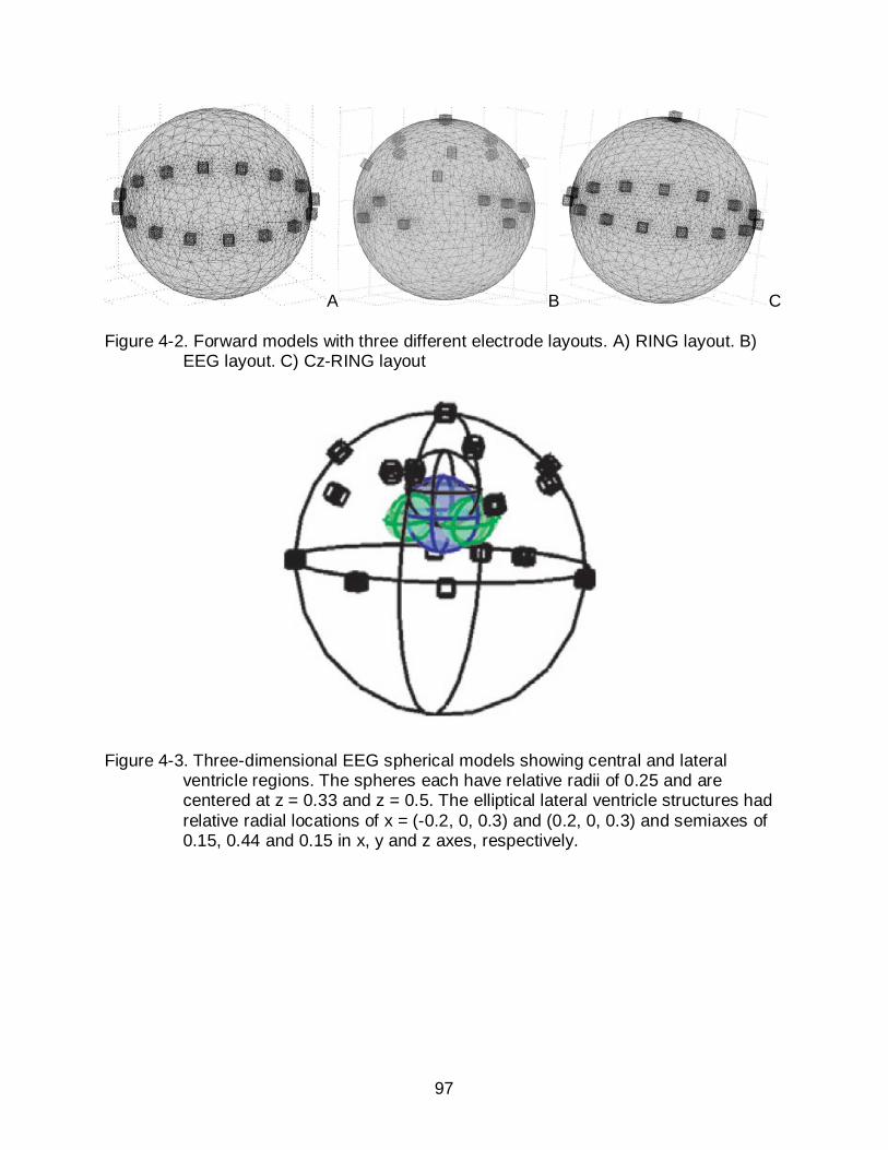
97
A B C
Figure 4-2. Forward models with three different electrode layouts. A) RING layout. B) EEG layout. C) Cz-RING layout
Figure 4-3. Three-dimensional EEG spherical models showing central and lateral ventricle regions. The spheres each have relative radii of 0.25 and are centered at z = 0.33 and z = 0.5. The elliptical lateral ventricle structures had relative radial locations of x = (-0.2, 0, 0.3) and (0.2, 0, 0.3) and semiaxes of 0.15, 0.44 and 0.15 in x, y and z axes, respectively.

98
.
Figure 4-4. A model with an outer brain shell and a central region of CSF (Model A) viewing from the top. The anomaly positions on the mid xy plane (equator plane) are demonstrated. Other anomaly positions are distributed the same way on the mid yz plane and mid zx plane. There are totally 37 anomaly positions within the central region of CSF. The anomaly has a relative radius of 0.05. This model was used with each of the three electrode layouts
A B
Figure 4-5. A more complex model (Model B) with scalp, brain, ventricles and skull shells, including a structure similar to the fontanel (highlighted). A) Top view, demonstrating that a blood-like anomaly with a relative radius of 0.1 was moved over to the 6 positions within the ventricles. B) Side view, demonstrating that the ventricles were placed at a relative radius 0.3 above the equator. This model was used with the RING layout and EEG layout only
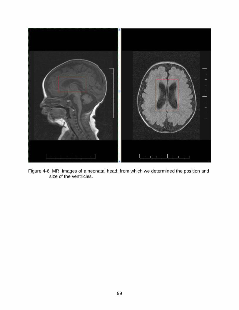
99
Figure 4-6. MRI images of a neonatal head, from which we determined the position and size of the ventricles.
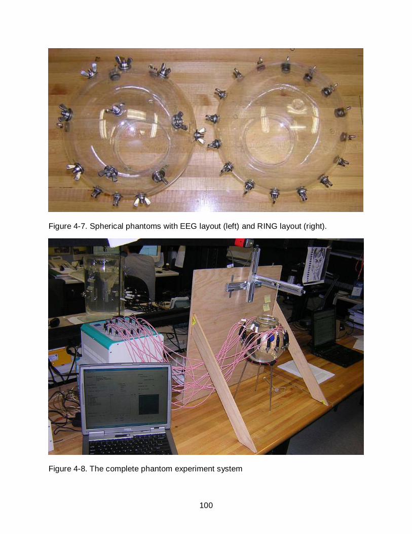
100
Figure 4-7. Spherical phantoms with EEG layout (left) and RING layout (right).
Figure 4-8. The complete phantom experiment system
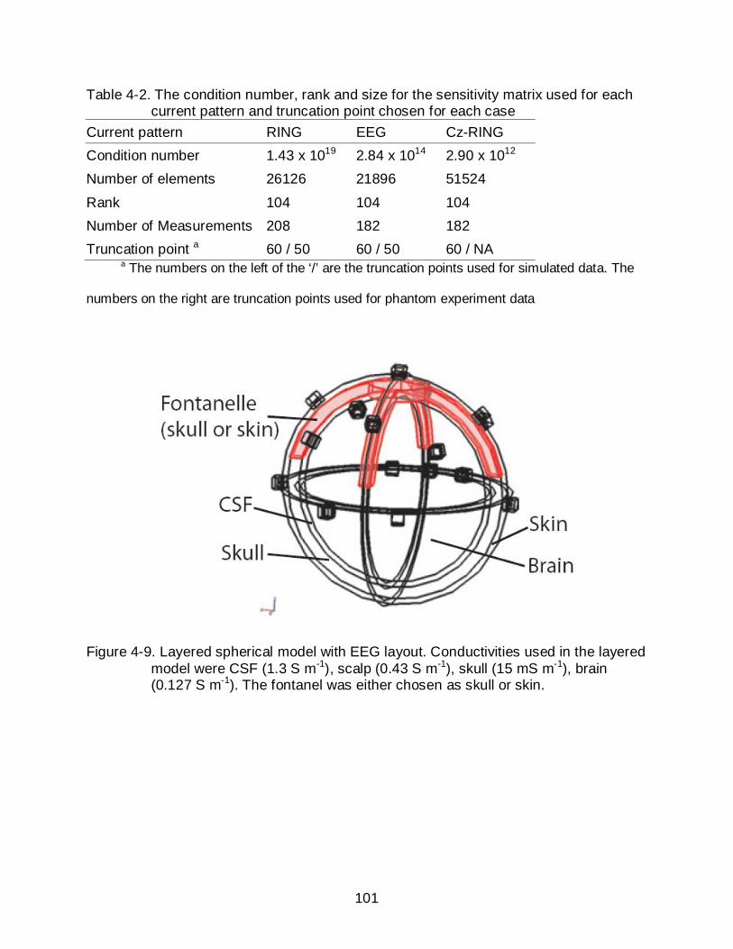
101
Table 4-2. The condition number, rank and size for the sensitivity matrix used for each current pattern and truncation point chosen for each case
Current pattern RING EEG Cz-RING Condition number 1.43 x 10¹⁹ 2.84 x 10¹⁴ 2.90 x 10¹² Number of elements 26126 21896 51524
Rank 104 104 104 Number of Measurements 208 182 182 Truncation point a 60 / 50 60 / 50 60 / NA
a The numbers on the left of the ‘/’ are the truncation points used for simulated data. The
numbers on the right are truncation points used for phantom experiment data
Figure 4-9. Layered spherical model with EEG layout. Conductivities used in the layered model were CSF (1.3 S m-1), scalp (0.43 S m-1), skull (15 mS m-1), brain (0.127 S m-1). The fontanel was either chosen as skull or skin.

102
Figure 4-10. Average sensitivities, calculated as a fraction of maximum values observed over the domain, for EEG, Cz-RING and RING patterns in the regions of interest. A) upper sphere; B) lower sphere; C) left ventricle; D) right ventricle.
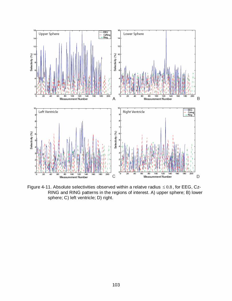
103
Figure 4-11. Absolute selectivities observed within a relatve radius 0.8≤ , for EEG, Cz-RING and RING patterns in the regions of interest. A) upper sphere; B) lower sphere; C) left ventricle; D) right.

104
A B
Figure 4-12. Radial relative localization errors for simulations on model A. A) Radial relative localization errors in the xy plane ( xyD ) at 37 different locations for the three current patterns on model A. B) Radial relative localization errors in the z direction ( zD ) at 37 different locations for the EEG pattern and Cz-RING pattern on model A. In both plots, the points in the left shaded area are the locations above the equator plane (1~10). The points in the central shaded area are the locations on the equator plane (11~27). The points in the right shaded area are those below the equator plane (28~37).
Figure 4-13. Quantification Indices of the 37 different anomaly positions for each of the three current patterns on model A. The 37 QIs for each case were normalized with respect to their average. Points in the left shaded area correspond to locations above the equator plane (1~10). The points in the middle shaded area correspond to locations on the equator plane (11~27). Points in the right shaded area correspond to points below the equator plane (28~37).
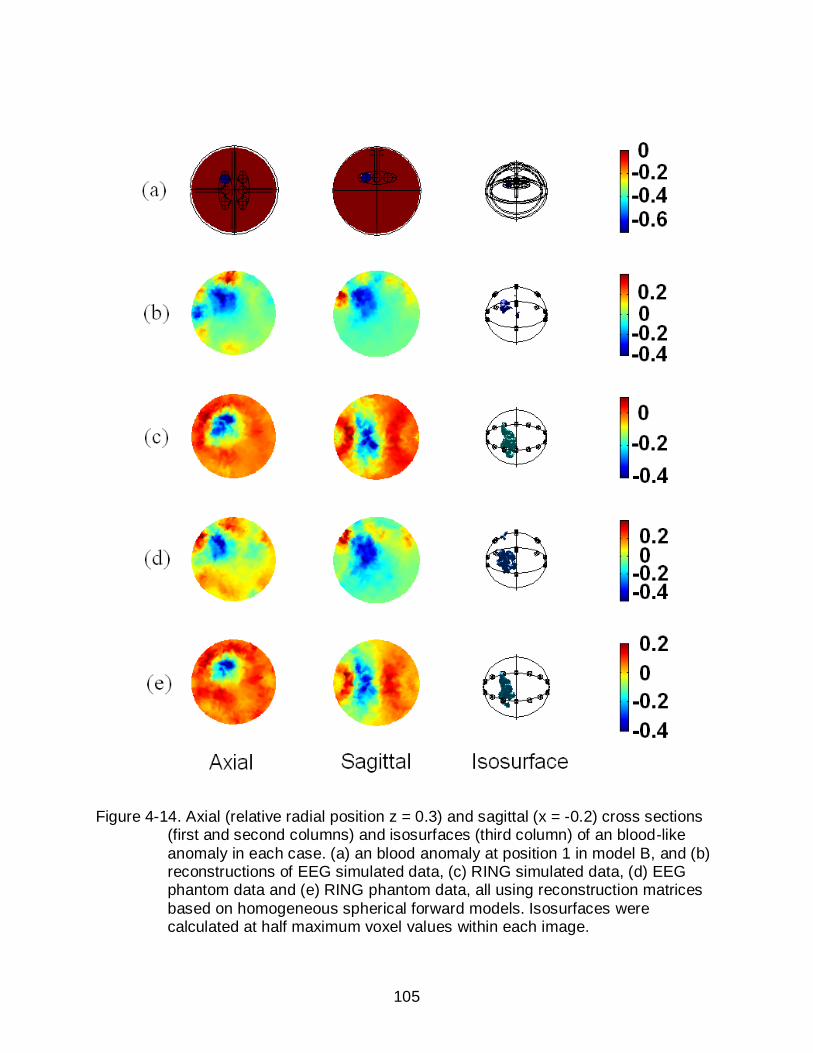
105
Figure 4-14. Axial (relative radial position z = 0.3) and sagittal (x = -0.2) cross sections
(first and second columns) and isosurfaces (third column) of an blood-like anomaly in each case. (a) an blood anomaly at position 1 in model B, and (b) reconstructions of EEG simulated data, (c) RING simulated data, (d) EEG phantom data and (e) RING phantom data, all using reconstruction matrices based on homogeneous spherical forward models. Isosurfaces were calculated at half maximum voxel values within each image.
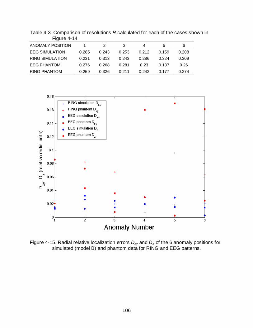
106
Table 4-3. Comparison of resolutions R calculated for each of the cases shown in Figure 4-14
ANOMALY POSITION 1 2 3 4 5 6 EEG SIMULATION 0.285 0.243 0.253 0.212 0.159 0.208 RING SIMULATION 0.231 0.313 0.243 0.286 0.324 0.309 EEG PHANTOM 0.276 0.268 0.281 0.23 0.137 0.26 RING PHANTOM 0.259 0.326 0.211 0.242 0.177 0.274
Figure 4-15. Radial relative localization errors Dxy and Dz of the 6 anomaly positions for simulated (model B) and phantom data for RING and EEG patterns.
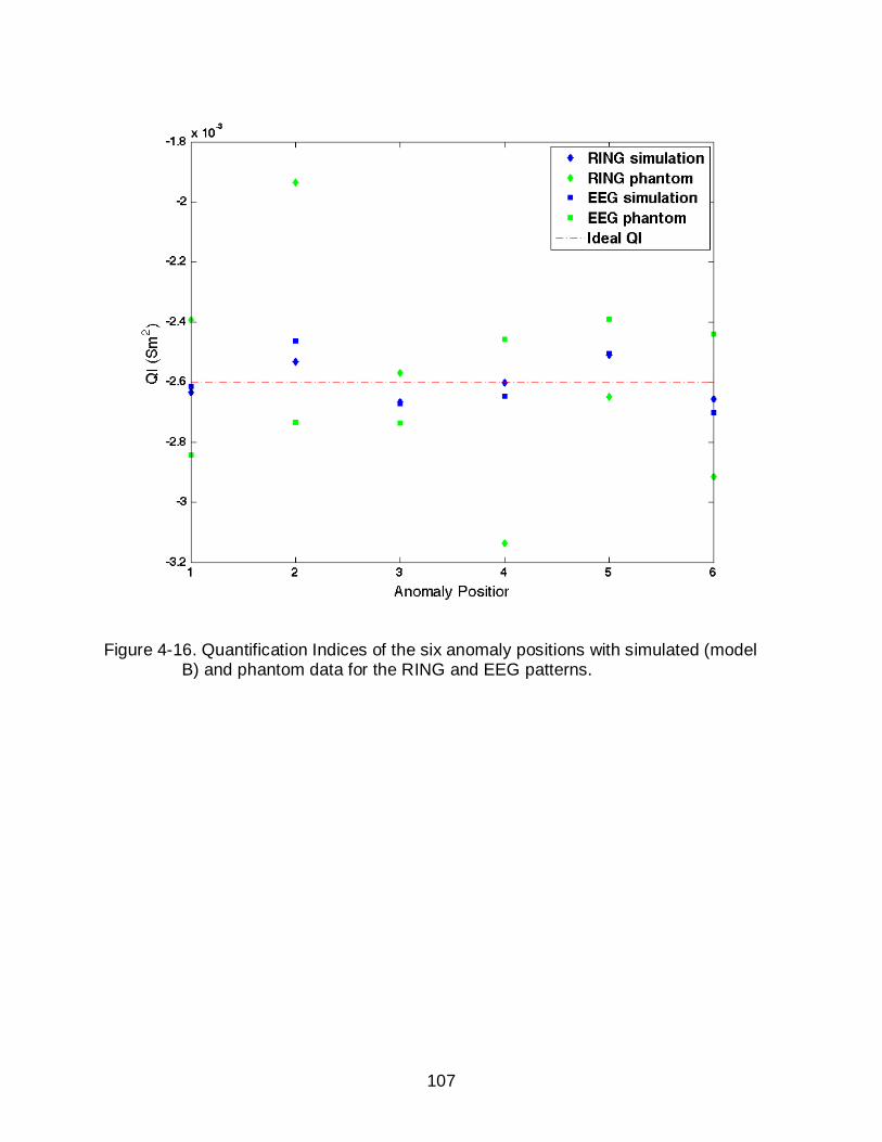
107
Figure 4-16. Quantification Indices of the six anomaly positions with simulated (model B) and phantom data for the RING and EEG patterns.

108
Figure 4-17. Comparisons between ‘open-skull’ and ‘closed-skull’ reconstructions. Axial (Relative radial position of z = 0.3) and sagittal (x = -0.2) cross sections (first and second columns) and isosurfaces (third column) showing (a) ideal image of bleeding at position 1 within a spherical model, and the reconstructions using the EEG current pattern on ‘open skull’ or ‘closed skull’ models at three different noise levels. The noise levels used were 50dB (b) open skull and (c) closed skull, 65dB (d) open skull and (e) closed skull and 75dB (f) open skull and (g) closed skull. Isosurfaces were calculated at half maximum voxel values within each image.

109
CHAPTER 5 STUDIES USING A REALISTIC HEAD-SHAPED MODEL
Background
So far we have found a robust current pattern (the EEG pattern) using spherical
neonatal head models. However, real neonatal heads differ from spherical models in
many aspects, such as their external boundary shape and internal anatomical
structures. Due to the ill conditioning of the EIT problem, these differences will introduce
errors to the reconstructed images when applying the spherical algorithm on data
collected from real patients. To investigate the true quality of the EEG current pattern on
real subjects and our spherical reconstruction algorithm, we performed studies using
neonatal head models with realistic boundary geometry and major anatomical
structures.
Some previous studies demonstrated that an incorrect estimate of boundary shape
will reduce the quality of the reconstructed image through the introduction of artefacts
(McInerney and Terzopoulos 1996). Incorporating an accurate forward model instead of
using circular or spherical forward models has been a popular problem in brain imaging
(Bagshaw et al. 2003, Liston et al. 2004) and lung imaging (Borsic et al. 2001, Fan et al.
2009). All the earlier studies showed that the image quality could be generally improved
using such approaches, which are especially useful for absolute EIT imaging. However,
realistic models need to be used carefully, because with inaccurate prior information,
they may yield images worse than reconstructed with a simple forward model (Liston et
al. 2004). In practice, head geometry varies from patient to patient, which makes it
difficult to accurately specify the forward model. In addition, the neonatal head can vary
in shape depending on posture. In this study, we compared the images reconstructed

110
using a spherical forward model and a head-shaped forward model and evaluated the
necessity of using an accurate forward model for the purpose of detecting and
quantifying intraventricular bleeding in neonates.
Methods
The Neonatal Head-shaped Model
A 3D numerical neonatal head model (Figure 5-1) was provided by Dr. Richard
Bayford and Dr. Andrew Tizzard from Middlesex University, UK. This model (the RG
model) contained 4 different anatomical structures (skin, skull, CSF and brain) which
were manually segmented from MRI images of a normal term neonate (Figure 5-2)
(Tizzard et al. 2005). The total volume of the model was 791 ml. The RG model was
meshed into 45702 tetrahedral elements with 8703 nodal points (the RG mesh). We
implemented the 16 EEG electrode layout on top of the scalp based on their spherical
coordinates. Electrode locations were chosen to be as similar as possible to those used
on the spherical background model while adapting to the realistic head’s orientation.
The Cz electrode was shifted off the central axis to determine the effect of electrode
location variation on model’s symmetry. The mesh data can be organized into a file with
STL format or MPHTXT format, and then imported into COMSOL for the purpose of
geometry visualization and numerical simulation.
Sensitivity Analysis
Similar to the analysis done with the spherical models in Chapter 4, sensitivity
analysis was also done for a homogeneous RG model equipped with the EEG electrode
configuration. This could help to determine the extent of differences that would be
expected using this method in vivo. In making comparable regions to those in spherical
models, we averaged maximal x, y and z deviations from the model anatomic center

111
and used these values to calculate approximate elliptical semiaxes for the model. These
values were then used to create elliptical regions with the same relative locations and
semiaxis values to those used in spherical background models (Figure 5-5). These
regions are illustrated in Figure 5-3. Volumes of 11.1 ml and 11 ml were calculated from
lower and upper central regions, respectively. Both left and right ventricle volumes were
about 4.2 ml, similar to those observed in vivo (Gilmore et al. 2001). The sensitivity
matrix calculated using the EEG layout on a uniform realistic geometry model had
45702 elements, and had a condition number of 56.3 10× . As for all other models, its
rank was 104.
Simulation of IVH
To simulate intraventricular bleeding, we added two ventricles within the brain
compartment of the RG model. Similar to the ventricle structures used in the spherical
model, they were elliptical with a total size of about 1/70 of the head volume. The
ventricles were placed 18 mm above the anatomical center and were spaced laterally
18 mm apart about this point. We used 6 bleeding sites at similar relative locations
within the ventricle regions, as for the spherical model (Figure 5-4). Tissue
conductivities used were the same as for the spherical model (blood 0.67 S/m, CSF 1.3
S/m, brain 0.17 S/m, scalp 0.43 S/m, skull 0.06 S/m). To get a more comprehensive
understanding of quantification in this RG model, we also investigated multi-site
bleeding. To do this we placed anomalies at combinations of the 6 locations, leading to
a total of 1 2 3 4 5 66 6 6 6 6 6 63C C C C C C+ + + + + = bleeding cases.

112
Investigation of Boundary Shape Mismatch
In this study, we focused on investigating the effect of model boundary geometries
on reconstructed images. More precisely, we compared image qualities and
quantification accuracies in the head using a spherical forward model and a realistic
geometry forward model.
Forward models
Two forward models were used to formulate the sensitivity matrices. One was a
spherical model with unit radius and homogeneous conductivity distribution (the SP
matrix), which has been used through out the studies in Chapter 4. The other was a
neonatal head model with realistic head geometry and homogeneous conductivity
distribution (the RG matrix), which is the same as the homogeneous RG model used
earlier for sensitivity analysis.
Data generation
We gathered simulated bleeding data using three different head-shaped finite
element models and one head-shaped phantom. The first one (the M model) (Figure 5-5
A) had a boundary geometry the same as the RG model we used to formulate the RG
sensitivity matrix. The background conductivity was assigned to be homogeneous with
the conductivity of CSF (1.3 S/m). In this study, we created two bleeding sites at
positions corresponding to the centers of the left and right ventricles, respectively.
Bleeding was simulated by manually setting the corresponding elements of the finite
element forward model to the conductivity of blood (0.67 S/m). The centers of the
ventricles were the same as used in Figure 5-4. We simulated 6 different cases on each
side with total blood volume increasing linearly from 0.5 ml to 3 ml.

113
To test our methods in the presence of realistic noise, we constructed a plastic
head-shaped phantom of the M model, using a 3D printer (Dimension, Inc., MN, USA).
The procedures to construct the phantom are illustrated in Figure 5-6. The surface
mesh was first extracted from the M model, with the bottom surface removed. The mesh
was therefore hollow at the ‘neck’. We then produced a copy of the mesh at 90% of its
original scale, and placed it inside the original mesh. By connecting the two bottom
‘circles’ at the neck with triangles, we created a closed shell-like structure with a
triangular surface mesh. The surface mesh information was then saved into a STL
format file, and imported into the 3D printer. It took 20 hours for the 3D printer to
construct the phantom.
The phantom had the same boundary shape as the M model, but its total volume
was 1628 ml, about twice the actual model volume. The phantom had 16 stainless steel
electrodes attached as shown in Figure 5-5 B. A 0.6% saline solution (the conductivity
of which was approximately 1.3 S/m, the conductivity of CSF) was used as the phantom
background. Bleeding was simulated using gel anomalies made of TX151, agar and
saline. The TX-151 gel conductivity was adjusted to 0.67 S/m. We made 6 cylindrically-
shaped anomalies with volumes from 1-6 ml. Following the simulated data generated
from model M, we placed gel anomalies at the left and right ventricle centers, which
were determined to be 23 mm above the anatomical center and 23 mm apart from each
other. Anomalies were placed accurately using a 3D positioner (Velmex, Inc., NY, USA).
Data was collected using the KHU Mark1 EIT system. We chose to use a single
frequency of 10 kHz and a constant current output of 1 mA. Ten data sets were
collected and averaged as a reference before anomalies were introduced. In each of

114
the 12 experiments, ten data sets were collected and averaged as the perturbation data
for that volume of bleeding.
The other RG model used in this study (model G) (Figure 5-5 C) was provided by
researchers at the University of Gent in Belgium. It was constructed from the MRI data
from a 39 week gestational age patient who suffered from asphyxia. The original 3D
image had a dimension of 256 x 256 x 129, with each pixel size 0.7 x 0.7 x 0.63 mm.
Five major structures were segmented from the images, including CSF, brain tissue,
skull, fat and scalp (Figure 5-7).
Theoretically, we could use the original image as a rectangular brick mesh to
obtain FEM solutions. However, the original image contains 75 10× elements. Our
experience told us that problems around this size would be very computational costly.
To speed up the simulation process, we reduced the image size by grouping each 5 x 5
x 5 block as one pixel. The image dimension was therefore reduced to 51 x 51 x 26.
The process was performed very carefully to make sure the skull structures were
preserved and closed in all slices. To acquire more accurate FEM solutions, we decided
to convert the mesh elements to tetrahedrons. Each rectangular brick was divided into 6
tetrahedrons in the manner shown in Figure 5-8. Of course this is not the only way to
divide a brick into tetrahedrons. However, we needed to keep in mind that adjacent
tetrahedrons have to share a common triangular face. So we divided the bricks such
that the diagonal lines on the opposite sides of a brick had the same orientation. The
mesh finally contained 23920 nodes and 126432 tetrahedrons.
The purpose of using this model was to test our two sensitivity matrices on a
different ‘patient’, whose geometry matched neither one of the forward models. In the

115
beginning of this study, we were primarily interested in the effects from boundary shape.
Therefore, we removed the internal structures by setting the background homogeneous
with conductivity value 1.3 S/m (uniform G model) and selected two bleeding sites at the
ventricle centers. Ventricle center positions were determined using the original MRI
data. We determined that the two ventricles were 44 mm above the base and 17 mm
apart. We simulated six different cases each side with blood volumes increasing linearly
from 0.5 ml to 3 ml. The 16 EEG electrodes were also incorporated on the scalp
according to their spherical positions. After that we decided to make this model more
realistic. Therefore we put all the structures back into the model (layered G model), as
shown in Figure 5-7. The positions and volumes of simulated bleeding were the same
as used in the uniform G model.
Results
Sensitivity Analysis
Figure 5-9 shows the sensitivities and selectivities for the EEG pattern in simulated
ventricles and upper and lower spheres of the homogeneous RG model. These figures
may be compared directly with the EEG pattern results obtained for the uniform
spherical model in Chapter 4. Both sensitivities and selectivities were very similar to
those observed in the spherical model. Volumes of central regions were around twice
the ventricle volumes in the RG model and this is reflected in the absolute selectivity
plots. The relatively large sensitivity and selectivity in the left ventricle likely reflects the
asymmetry of Cz electrode placement. Maximum selectivities in the realistic geometry
sensitivity matrix were similar in all four regions to those found for the spherical model
matrix, but fewer large selectivities were observed.

116
Layered RG Model
We compared images reconstructed using a sensitivity matrix calculated from the
homogeneous spherical model ( SPS ) and a sensitivity matrix calculated from the
homogeneous RG model ( RGS ). Data was generated from the layered RG model shown
in Figure 5-2. Figure 5-10 shows the reconstructions for an individual impedance
change at position 1. Images in Figure 5-10 reconstructed using the spherical matrix
were similar to the second image in Figure 5-14, which shows the reconstruction from
EEG data calculated from a spherical object. Although resolutions were better for RG
reconstructions than for spherical (0.138 and 0.168 respectively), the contrast for the
spherical case (0.467) was better than for RG reconstructions (0.454).
To further investigate the resolution for images reconstructed using SPS , we
compared reconstructions of anomaly pairs 1-4, 2-5, 3-6 and 1-6 (refer to Figure 5-4 for
anomaly positions). In each of the 4 cases, the two anomalies were located at different
sides of the ventricles. This way we could test the ability of the spherical matrix to
discriminate bleeding locations when there was bleeding in both ventricles. As a criteria
for successful anomaly resolution, we required that the conductivity values
reconstructed on the line joining the anomalies should dip to less than half the
maximum value observed in either anomaly. The anomaly profiles are shown in Figure
5-11. We found that anomalies 1-4 and 1-6 and 3-6 were resolvable but not 2-5.
Quantification results for multi-site bleeding cases are compared in Figure 5-12.
The correspondence between results obtained using the spherical reconstruction matrix
were similar to those obtained from the realistic geometry matrix: both of them giving QI
estimations having a maximum error no more than 0.0025 S.cm2 over all positions, a

117
value that corresponds to a blood volume of 0.4 ml when considered relative to the total
volume of the head. We also compared the performance of the two reconstruction
matrices with respect to QI values when white Gaussian noise was added to data
(Figure 5-13). In this figure we compare the average and standard deviation of QI errors
over all positions for both reconstruction matrices at 11 different SNR levels between 60
and 90 dB. We found that the variation in quantification errors became almost 3 times
larger for both reconstruction methods as the SNR was decreased to 60 dB.
Investigation of Boundary Geometry Effects Using Homogeneous RG Models
Reconstructions of anomaly 1 are shown for model M (Figure 5-14 A), uniform
model G (Figure 5-14 C) and layered model G (Figure 5-14 D). Only reconstructions of
anomaly 6 are shown for model M phantom data (Figure 5-14 B) because reconstructed
images of anomaly 1 were severely contaminated by noise. Left and right
reconstructions were compared in each case to demonstrate asymmetry, and image
resolutions for all the reconstructed images are shown in Table 5-1. As expected, the
reconstructions from model M data using the RG matrix had consistently better image
resolutions than reconstructions using the SP matrix. The RG matrix also showed an
advantage over the SP matrix in reconstructing model M phantom data. However, the
RG matrix did not show a consistent advantage in reconstructing data from the uniform
model G. Instead, the SP reconstructions had consistently better image resolutions
(average R = 0.1887) than the RG reconstructions (average R = 0.2168) for the right
side, although the RG reconstructions showed better image qualities (average R =
0.1836) than the SP cases (average R = 0.2929) for the left side. RG reconstructions for
the layered model G data showed better image resolutions in most cases, except for
blood volume 1 on the right side.

118
Quantification indices for the 6 different anomaly sizes on the left side were
calculated for each of the four models (Figure 5-15). The results for the anomalies on
the right side were similar. The quantification performances of the two matrices were
almost identical for simulated model M data. The RG matrix had a relatively better
quantification accuracy for model M phantom data (average error = 0.0025 S.cm2),
compared with the SP matrix (average error = 0.0034 S.cm2). The RG matrix did not
show any significant advantage over the SP matrix for the data from uniform model G
and layered model G.
Discussion
Sensitivity analysis on the realistic geometry model showed that the sensitivity and
selectivity patterns using the EEG electrode configuration on this model were similar to
those obtained from the spherical model. This further indicated the potential of using the
EEG method on real patient subjects.
Studies using the layered realistic geometry model (Figure 5-2) showed the
possibility of using a spherical forward model to reconstruct images using data collected
from a real head. A number of earlier studies showed that incorporating a more
accurate forward model that matches the conductivity structures of the imaged object
can improve image quality in general. For example, inclusion in forward models of a
bone model (Meeson et al. 1995), a four-shell head model (Bagshaw et al. 2003) or
including anisotropy (Abascal et al. 2008) all demonstrated improvements in image
quality, image resolution and localization errors. However, if the prior information within
the realistic model is not accurate enough, they may yield images worse than those
reconstructed with a simple model (Liston et al. 2004). In Bagshaw et al. (2003), it was
noted that using a full-shelled head model produced worse images than using the

119
homogeneous head model when reconstructing the head phantom data, because the
resistivity ratio between the skull and brain region for the tank was too dissimilar to the
value assumed in the model. Meeson et al. (1995) also concluded that using a uniform
matrix seems less likely to generate artifacts when the underlying conductivity
distribution is unknown. Bagshaw et al. (2003) also studied the effect of using realistic
geometry in the forward model. They found that both localization accuracy and image
quality was improved, but only slightly. In practice, head geometry varies from patient to
patient, which makes it difficult to find a forward model that is really accurate, unless
each model is constructed individually. However, constructing patient specific models
may not be quite possible due to the difficulty of collecting high quality MR images from
neonates. Exactly how accurate a model should be is a matter of discussion (von
Ellenrieder et al. 2006). Therefore, it is of great interest to investigate the quality of
reconstructions and quantity index accuracy using a homogeneous spherical model as
a forward model. Figure 5-12 shows that the QIs calculated using the spherical matrix
were similar to those calculated using the accurate RG matrix with a maximum error of
0.0025 S.cm2 (0.4 ml) in both cases. The response curve was not exactly linear, and
appeared to have a zero intercept at a volume larger than 0 ml. This suggests that
sensitivity is low at very small volumes. Both spherical and RG matrix results tended to
shift away from the expected QI when the total blood volume became larger than 1.5 ml.
This tendency agreed with the observations from (Sadleir et al. 1998) when using
anomalies less conductive than the background. Both these inaccuracies may be
caused by the nonlinear characteristics of the EIT problem itself (Seagar et al. 1987). As
Figure 5-13 shows, use of the RG reconstruction matrix did not produce an advantage

120
over the spherical reconstruction matrix at all SNR levels. The largest QI variability
found using the spherical matrix increased to 0.006 S.cm2 (corresponding to a blood
volume of 0.95 ml) at 60 dB. However, this level of variability is not likely to lead to an
incorrect diagnosis of type II IVH, in which the blood volume may be up to 3ml.
The studies using the three homogeneous models (the M model, M phantom,
uniform G model) and one layered model (layered G model) further proved the potential
of using spherical model as a generalized forward model for different patients. As
discussed earlier, EIT image quality is highly dependent on the forward model. Fan et
al. (2009) found that the human lung reconstruction was improved by using a boundary
model developed from 3D CT scan data. In our study, we found that better image
resolutions were obtained using the RG matrix when using both simulated and phantom
data from model M. This confirmed the findings from early studies, since the RG model
had exactly the same boundary shape and electrode locations in model and phantom.
When using data from model G, the RG matrix still produced better results for left-
located anomalies. This can be explained by the asymmetry of the Cz electrode in the
RG model. In the RG model, the Cz electrode was placed to the left of the head apex
and therefore produced relatively larger sensitivity and selectivity in the left ventricle
region, as shown in Figure 5-9 C and D. However, the advantage for the RG matrix was
not sustained for anomalies positioned on the right, and here the SP matrix showed
consistent better image resolutions. Kolehmainen et al. (1997) and Blott et al. (1998)
concluded that the locations of electrodes and the boundary shape of the forward model
brought the most difficulties for the reconstructed images. The three homogeneous
models used in this study also enabled us to investigate the effect from boundary

121
geometries alone. The layered model G enabled us to compare the performance of the
two sensitivity matrices on a more ‘realistic’ patient. An interesting finding was the
relative performance of the RG matrix improved compared to its performance on the
uniform G model, although it did not show much advantage for small blood volumes.
Future work should include collecting data from real patients to validate these findings.
The RG matrix showed no better performance than the SP matrix in term of
quantification. Figure 5-15 A shows that the SP matrix could be calibrated to quantify
the anomalies as well as the RG matrix and these QIs matched the ideal QIs. The RG
matrix did not show consistent advantage with model M phantom data (Figure 5-15 B).
Another interesting observation was that the QIs calculated from the SP matrix showed
smaller error bars in most cases, which indicates that the SP matrix may have an
advantage over the RG matrix in a noisy environment. Both matrices quantified data
from the uniform model G well (Figure 5-15 C). In this case, where the object geometry
matched neither sensitivity matrix, the RG matrix did not show any advantage over the
SP matrix. When looking at the quantification result from the layered model G (Figure 5-
15 D), we found that the QIs from RG matrix showed slightly better accuracy when the
blood volume was getting large. However, this did not seem to give a significant
advantage for the detection of grade II IVH.
The spherical matrix reconstructions could of course not localize anomalies as well
as the RG matrix cases. However, images reconstructed with the spherical matrix
showed the anomalies coherently, and allowed us to verify their location — something
that could be of practical benefit in verifying diagnoses made from QI information. In
considering whether it is appropriate to use RG or spherical models for diagnosis in this

122
application, it is important to bear in mind the hazards inherent in obtaining RG data in
unstable neonates (involving transport to MRI or CT machine and the inherent risks
during these steps, as well as the time needed to produce an RG model) and weighing
them against the clinical need to confirm bleeding. It is probably true that use of a
reconstruction based on an appropriate geometry will produce better images. However,
we have shown here that postprocessing of images using both methods obtained
similarly accurate QI values. If QI is used as a primary indication of bleeding status,
images could be used as a secondary measure to verify the presence of a coherent
anomaly and to discount the possibility of QI variations being caused by electrode
contact problems or other equipment errors. While images from spherical
reconstructions are not quite as clear as in those based on accurate models of the
head, sufficient information should be present in these reconstructions to allow
verification of diagnoses.
Conclusion
We further investigated the performance of the EEG method using a head model
with realistic geometry and anatomical structures. The results indicated the potential of
using this method in real clinical trials. We also compared the performance of two
sensitivity matrices ( SPS and RGS ) using different head models. It is evident that the
matrix developed from a realistic-shaped forward model does not guarantee image
quality when the subject has mismatched boundary shape and electrode locations.
Moreover, the SP matrix performed better in quantification of phantom experiment data.
All our observations indicate that using a simple spherical matrix might be adequate for
monitoring IVH in neonates.
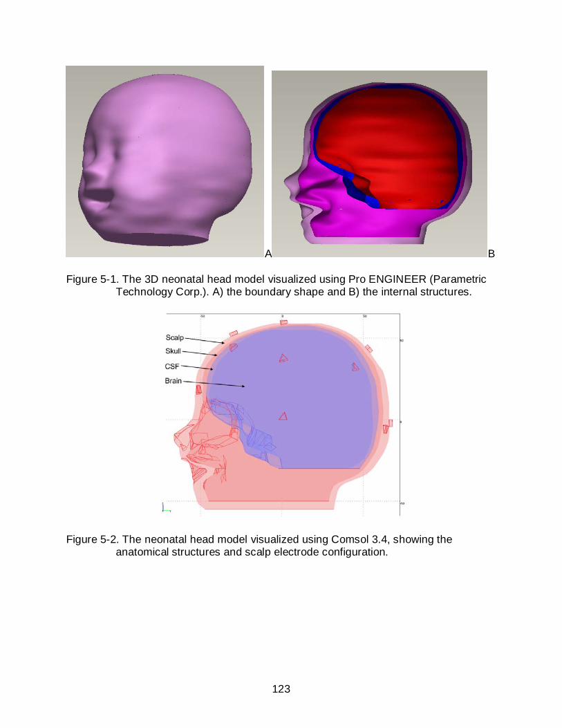
123
A B
Figure 5-1. The 3D neonatal head model visualized using Pro ENGINEER (Parametric Technology Corp.). A) the boundary shape and B) the internal structures.
Figure 5-2. The neonatal head model visualized using Comsol 3.4, showing the anatomical structures and scalp electrode configuration.
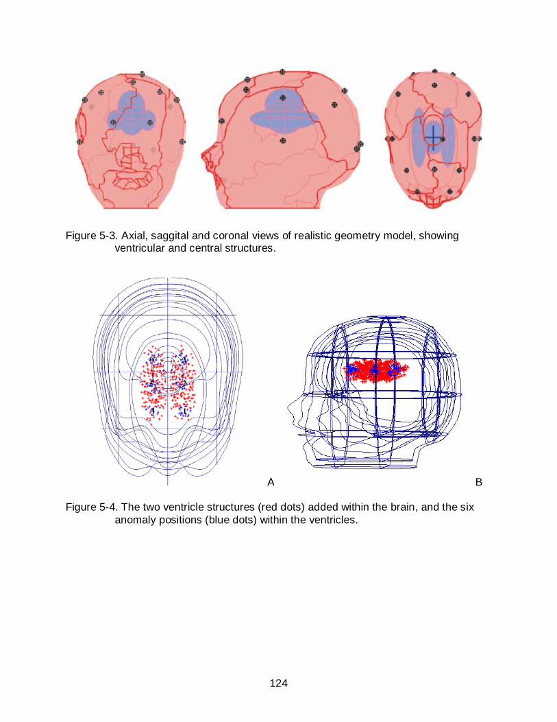
124
Figure 5-3. Axial, saggital and coronal views of realistic geometry model, showing ventricular and central structures.
A B
Figure 5-4. The two ventricle structures (red dots) added within the brain, and the six anomaly positions (blue dots) within the ventricles.
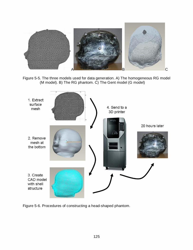
125
A B C
Figure 5-5. The three models used for data generation. A) The homogeneous RG model (M model). B) The RG phantom. C) The Gent model (G model)
Figure 5-6. Procedures of constructing a head-shaped phantom.
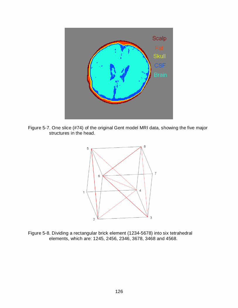
126
Figure 5-7. One slice (#74) of the original Gent model MRI data, showing the five major structures in the head.
Figure 5-8. Dividing a rectangular brick element (1234-5678) into six tetrahedral elements, which are: 1245, 2456, 2346, 3678, 3468 and 4568.
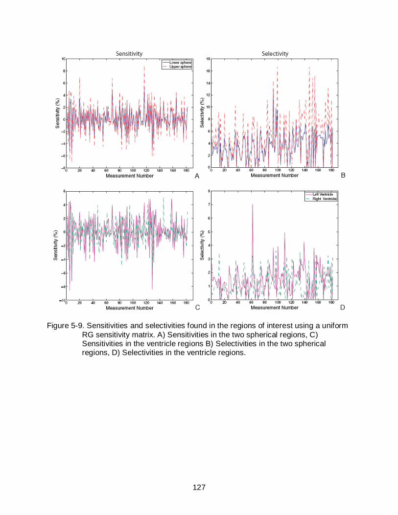
127
Figure 5-9. Sensitivities and selectivities found in the regions of interest using a uniform RG sensitivity matrix. A) Sensitivities in the two spherical regions, C) Sensitivities in the ventricle regions B) Selectivities in the two spherical regions, D) Selectivities in the ventricle regions.
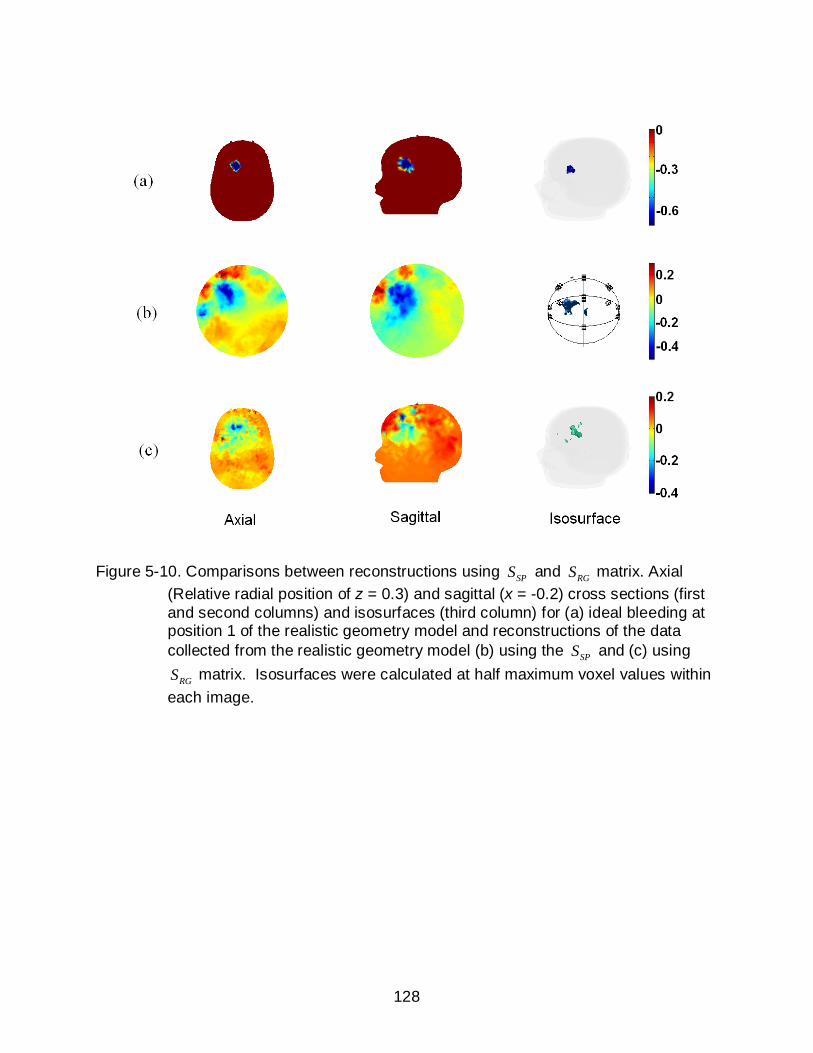
128
Figure 5-10. Comparisons between reconstructions using SPS and RGS matrix. Axial (Relative radial position of z = 0.3) and sagittal (x = -0.2) cross sections (first and second columns) and isosurfaces (third column) for (a) ideal bleeding at position 1 of the realistic geometry model and reconstructions of the data collected from the realistic geometry model (b) using the SPS and (c) using
RGS matrix. Isosurfaces were calculated at half maximum voxel values within each image.
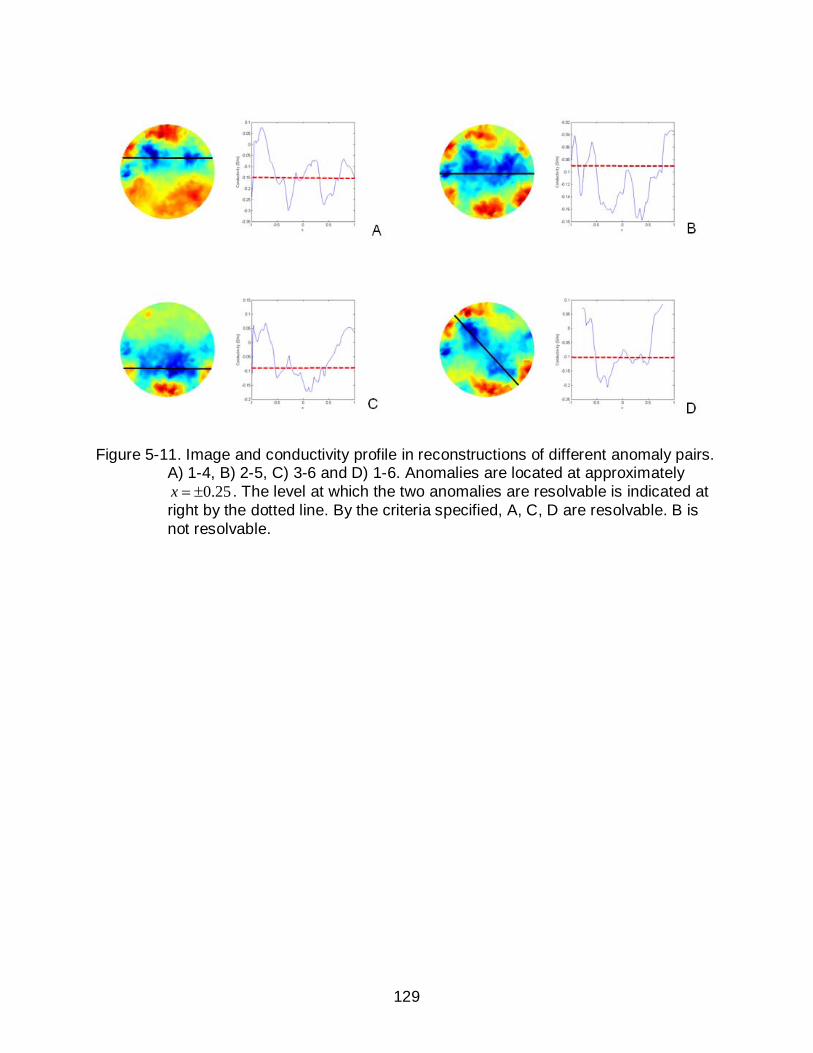
129
Figure 5-11. Image and conductivity profile in reconstructions of different anomaly pairs. A) 1-4, B) 2-5, C) 3-6 and D) 1-6. Anomalies are located at approximately
0.25x = ± . The level at which the two anomalies are resolvable is indicated at right by the dotted line. By the criteria specified, A, C, D are resolvable. B is not resolvable.
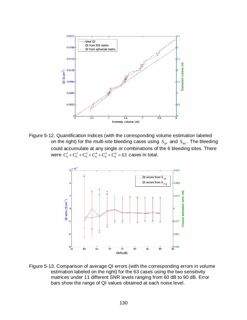
130
Figure 5-12. Quantification Indices (with the corresponding volume estimation labeled on the right) for the multi-site bleeding cases using SPS and RGS . The bleeding could accumulate at any single or combinations of the 6 bleeding sites. There were 1 2 3 4 5 6
6 6 6 6 6 6 63C C C C C C+ + + + + = cases in total.
Figure 5-13. Comparison of average QI errors (with the corresponding errors in volume estimation labeled on the right) for the 63 cases using the two sensitivity matrices under 11 different SNR levels ranging from 60 dB to 90 dB. Error bars show the range of QI values obtained at each noise level.
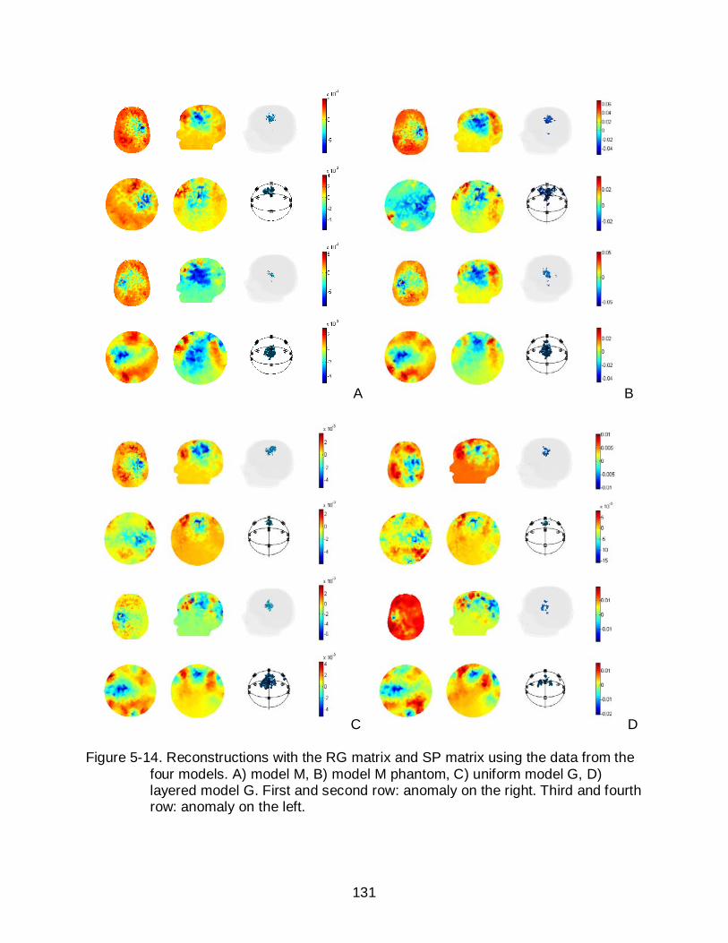
131
A B
C D
Figure 5-14. Reconstructions with the RG matrix and SP matrix using the data from the four models. A) model M, B) model M phantom, C) uniform model G, D) layered model G. First and second row: anomaly on the right. Third and fourth row: anomaly on the left.
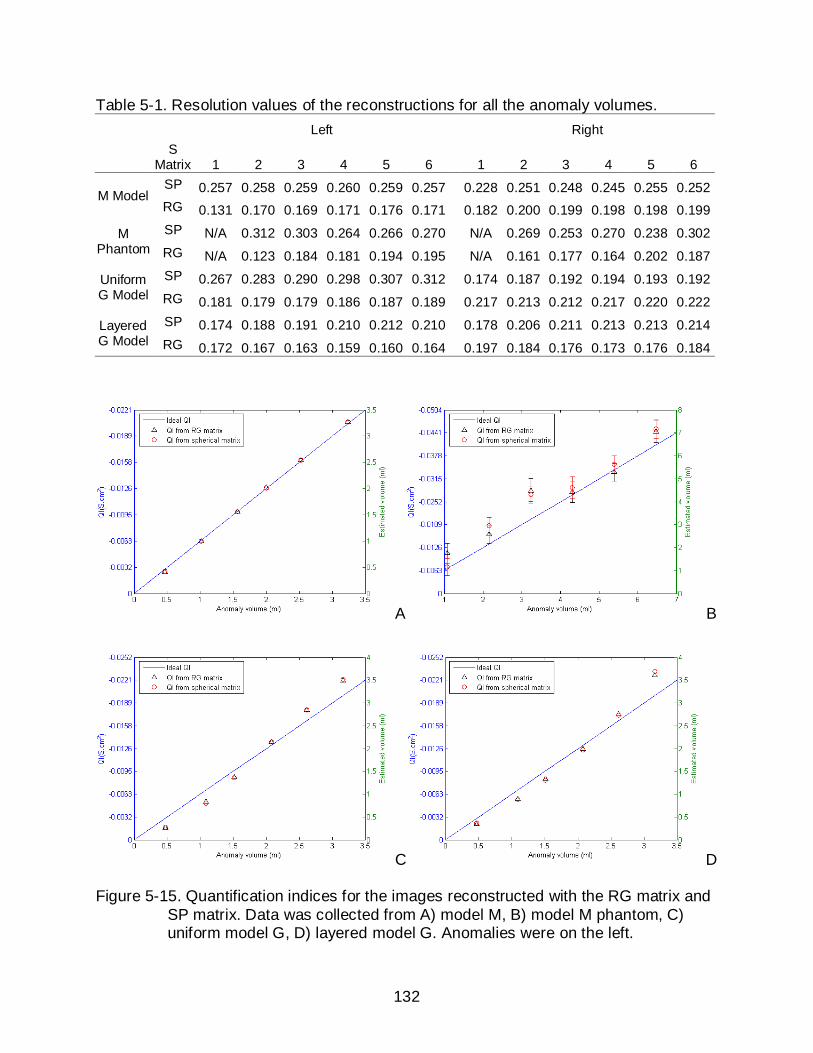
132
Table 5-1. Resolution values of the reconstructions for all the anomaly volumes. Left Right
S
Matrix 1 2 3 4 5 6 1 2 3 4 5 6
M Model SP 0.257 0.258 0.259 0.260 0.259 0.257 0.228 0.251 0.248 0.245 0.255 0.252 RG 0.131 0.170 0.169 0.171 0.176 0.171 0.182 0.200 0.199 0.198 0.198 0.199
M Phantom
SP N/A 0.312 0.303 0.264 0.266 0.270 N/A 0.269 0.253 0.270 0.238 0.302 RG N/A 0.123 0.184 0.181 0.194 0.195 N/A 0.161 0.177 0.164 0.202 0.187
Uniform G Model
SP 0.267 0.283 0.290 0.298 0.307 0.312 0.174 0.187 0.192 0.194 0.193 0.192 RG 0.181 0.179 0.179 0.186 0.187 0.189 0.217 0.213 0.212 0.217 0.220 0.222
Layered G Model
SP 0.174 0.188 0.191 0.210 0.212 0.210 0.178 0.206 0.211 0.213 0.213 0.214 RG 0.172 0.167 0.163 0.159 0.160 0.164 0.197 0.184 0.176 0.173 0.176 0.184
A B
C D
Figure 5-15. Quantification indices for the images reconstructed with the RG matrix and SP matrix. Data was collected from A) model M, B) model M phantom, C) uniform model G, D) layered model G. Anomalies were on the left.

133
CHAPTER 6 STUDIES USING PIGLET MODELS
Introduction
So far we have described promising results in numerical simulations and phantom
experiments. To validate the true quality of our method, we also performed experiments
on animal models.
An appropriate animal model is essential for research on human applications since
ethical considerations prohibit many investigations in humans (Baltzell et al. 1987).
Piglets have been chosen as animal models in many neonatal studies (Aquilina et al.
2007, Puiman and Stoll 2008, Jones et al. 2008), because of the anatomical,
physiological, immunological and metabolic similarities between piglets and human
neonates. Piglets have also been used in EIT applications in the study of hemorrhage
(Xu et al. 2007, You et al. 2008). Therefore, we also chose to use a piglet model in our
research to study intraventricular hemorrhage in neonates.
Methods
Piglet 1
The experiment on piglet1 was mostly a feasibility test for our EEG method. The
purpose of this experiment was to observe if we could see a correlation between the
signal change and saline injections. The head of the piglet was cut off after sacrifice
and the brain was removed for another study. We used the head cavity for our
experiment (Figure 6-1). As a consequence, this head was incomplete in terms of
surface geometry and anatomical structures. We used 50 mm ECG electrodes (Figure
6-2 A) and cut them to smaller size, then applied 16 of them to the scalp at their
approximate locations in the EEG configuration. Because the electrodes did not stick

134
well to the skin, we had to tape many down when adding the extra strain of the EIT
system cables. We made an artificial gel “brain” using TX151 and agar (Figure 6-2 B).
The conductivity of the gel was measured to be 0.6 S/m. The shape was modified
carefully so it could just fit into the brain cavity. A hole was made in the center of the
“brain” to create a cavity for saline injections. The head construction was first monitored
to obtain a reference data set that contained 20 measurements. A 4 ml bolus of saline
(conductivity 1.3 S/m) was injected into the cavity inside the brain. Another 4 ml was
injected 3 minutes later through the same location. Each injection was also measured
20 times.
Piglet 2 and 3
Two female piglets were sacrificed by exsanguination at approximately 1 week of
age under a protocol approved by the University of Florida Institutional Animal Care and
Use Committee (IACUC). The sacrificed animals were decapitated and moved to our
laboratory. In contrast to piglet 1, these two piglet heads were intact. We first removed
hair from the skin, and then marked the 16 electrode locations on the scalp using a
permanent marker. Markings for locations were made using scaled distance
measurements from nasion to the mid point between the ears and left to right jaw
distances. Sixteen 4 mm neonate EEG electrodes (Biopac Systems Inc.
www.biopac.com) were filled with electrode gel and fastened to the scalp with adhesive
rings (Biopac Systems Inc.) (Figure 6-3 A). Use of neonate-specific EEG electrodes
produced much better results in terms of adhesion compared to the ECG electrodes
used on piglet 1. Saline solution with conductivity 1.3 S/m was made by dissolving salt
at a concentration of approximately 6 g/L in water, which was the same as the saline we
used for phantom experiments in the earlier chapters. An artificial fontanel was then

135
created on the skull of piglet 3 (Figure 6-4 A). The procedure used for this was as
follows. The head was fixed in place using a table vise. The scalp was cut open in a ‘T’
shape, avoiding electrode markings. The skin underneath the ‘T’ shape was detached
from the skull carefully with a scalpel. We then held the scalp open with two hemostats,
taking care to detach the scalp from the skull as little as possible. However, we did need
enough skull area exposed to make an opening. A diamond-shaped hole was then
created with a bone saw at the intersection of saggital and coronal sutures. The scalp
flap was then replaced and sewn in place (Figure 6-4 B). Blood-equivalent saline was
injected near the ventricles on left and right sides. We added 5 drops of blue dye into
the 1 liter of saline used for piglet 3, so that we could dissect the brain after the
experiment and determine where the saline had been injected. In the case of piglet 2,
injections were made through the brain stem, and a total volume of 6 ml was injected to
the left side and 7.5 ml was injected to the right side. For piglet 3, injections were made
via the artificial fontanel, with injections made in increments of 0.5 ml every 30 seconds.
A total volume of 3.5 ml was injected to the right side and then 4 ml was injected to the
left side of piglet 3.
Piglet 4 (the MRI Piglet)
In vivo experiments are important because this is the only way we can assess how
our electrical measurements would be affected by physiological changes such as
breathing and heart beats. Another reason is that the fluid injected into the ventricles
would probably circulate differently in a live animal than in the post mortem
experiments. One problem we were facing was how to make the injections into the
ventricles. The ventricles in the piglet brain are tiny and it would have been hard to
locate the ventricles without any external assistance. We therefore constructed a ‘3D

136
guide’ to match the neonatal piglet head geometry. The direction and depth of blood
injections could then be accurately controlled. The procedures we used in making the
guide are described below. These procedures, together with the post mortem
experiment followed, were approved by the IACUC. The piglet (Figure 6-5 A) was
euthanized by administration of IV Sodium Pentobarbital (100 mg/kg). It was then
immediately delivered to the MRI room, and scanned with a 3T MRI machine (Figure 6-
5 B). A 3D piglet head model was then reconstructed, and a mold that perfectly
matched the head geometry was constructed with a guide attachment opening on top
(Figure 6-6 A). The direction of the guide opening pointed to one of the ventricles. We
constructed two guides using a ZPrinter310 3D printer (Z Corp., Burlington, MA, USA),
one for the left ventricle (Figure 6-6 B), and the other for the right ventricle. Each guide
was similar in geometry, only slightly differing in the orientation of the cylindrical
opening. The ventricle depths were also determined from the 3D model. We measured
that the distance from ventricle to the entry point on the scalp was 17 mm and the
distance from ventricle to entry point on the attachment was 66 mm in each case. A
range of metal attachments could be connected with the opening, each having a
diameter matched to a different catheter size to allow accurate placement. We chose
an 18 gauge attachment to facilitate guidance of the catheter guide wire.
The scanned piglet was then transported to our lab, where we performed another
post mortem experiment (Figure 6-7). The experimental procedures were very similar to
piglet 3, except that we did not make an artificial fontanel for piglet 4. The guide was not
used in this experiment. The needle was pushed directly through the scalp and skull
and we first injected 0.5 ml every 10 seconds to the right side of the brain. To estimate

137
the minimum amount of bleeding we could detect, we then injected saline at a rate of
0.1 ml every 10 seconds to the left side of the brain. The saline used in this experiment
had the conductivity of 0.67S/m.
Piglet 5
This was our first in vivo piglet experiment. All in procedures for this and the
following in vivo experiments were approved by IACUC. The piglet was first
anesthetized using isoflurane by mask. Body temperature and heart beat were
monitored throughout the experiment. Blood was removed from the piglet’s umbilicus
using an umbilical artery/vein catheter (UAC/UVC). A catheter with 0.05 inch inner
diameter and 0.08 inch outer diameter was then guided into the brain using a guideware
insertion technique (Appendix B), with the assistance from the 3D guide we made
earlier. The detailed experiment procedures are described in Appendix B. However, in
this first in vivo experiment we failed to obtain blood from the umbilicus. We actually
found the vein in the umbilicus successfully in the first place. We then decided to leave
it there and draw the blood right before making injections. However, blood clotted in the
UVC during the ventricular catheter insertion procedure and we were not able to draw
any blood into the syringe. Therefore, we ended up injecting saline in this experiment.
The saline was injected at the rate of 0.1 ml every 10 seconds.
Piglet 6
In this experiment we removed blood from the umbilicus immediately after it was
catheterized, and following placement of the ventricular catheter we successfully
injected blood into the ventricles. The head of the piglet was dissected and preserved in
10% formaldehyde for several weeks. The brain was dissected after its preservation so
we could verify where the blood was injected and clotted.

138
Piglet 7 and 8
These two experiments were performed on the same day. There were a few
improvements from the piglet 6 experiment. Bleeding was observed in piglet 6
experiment when inserting the first dilator into the brain. More bleeding was observed
when introducing the second dilator. The cause of bleeding was suspected to be the
entry path and the size of the dilators. Therefore, we made a new guide for introducing
the ventricular injection catheter. Using this new guide, the cannula entry point on the
skin was 14 mm away from the ventricles, comparing to 17 mm using the old guide.
Also we used a new type of catheter (Cole-Parmer, Illinois, USA) made of polyimide for
blood injection. This catheter also had an inner diameter of 0.05 inches, but a much
smaller wall thickness (0.002 inches) compared to the old one. Because of its smaller
outer diameter, we did not have to use the dilator any more. These improvements
largely reduced the extent of bleeding. Another improvement was that we drilled a hole
in the skull using a bone drill before introducing the cannula. This made it much easier
to insert the cannula into the brain. Therefore, we could control the entry point and
depth with more accuracy. Blood was injected at the rate of 0.2 ml per 10 seconds for
piglet 7 and 0.5 ml per 20 seconds for piglet 8.
Piglet 9 and 10
These two experiments were performed on the same day. The procedures were
very similar to the experiment on piglet 8, except that we used vetbond tissue adhesive
(3M Global Headquarters, MN, USA) on these two piglets. Vetbond was applied at the
brain entry point after the catheter was inserted in place. The reason for doing this was
to prevent blood from flowing back through the entry point when making injections. It
also helped to fix the catheter in place. Vetbond was also applied on the scalp along the

139
incisions to prevent any blood or CSF from flowing out of the skin. Blood was injected at
the rate of 0.5ml per 20 seconds for both piglets.
Results
Piglet 1
Due to the simple experiment setup and the ‘incomplete’ skull structure for piglet 1,
we had electrode contact problems which caused voltage overflows in the
measurements. Therefore, we were not able to reconstruct images for the saline
injected. However, we did observe doubled voltage changes for the second 4 ml
injection comparing to the first one. Figure 6-8 shows the 182 voltage changes for the
two saline injections.
Piglet 2 and 3
The reconstructed isosurface images shown in Figure 6-9 show the progression of
reconstructed data in the head as bloodlike saline was injected into the head of piglet 2.
The reconstructions clearly show an anomaly grows in size as more saline is added.
Plots of the quantity index derived from the image sequence as a function of added
saline volume showed a linear dependence of QI on volume (Figure 6-10).
The reconstructed isosurface images for Piglet 3 were shown in Figure 6-11 and
the QI values were plotted against injection time in Figure 6-12. Only reconstructions for
saline injections on the right were displayed for piglet 3. We first injected 3.5 ml on the
right. When we injected on the left, saline started to leak from the sutured scalp.
Therefore, we were not able to reconstruct images for the left side injections. However,
the leakage was reflected clearly in the QI plot (Figure 6-12).

140
Piglet 4
The reconstructed isosurface images for the total 2.5 ml injections to the right side
were shown in Figure 6-13. The QI values were plotted against injection time in Figure
6-14 A. We can see that the QI was always trying to return to the baseline after each
injection. The absolute QI values were on a different scale from the results for piglet 2
and 3. The trend was more clearly reflected in the QI curve for the 0.1 ml/ 10 s injection
on the left side (Figure 6-14 B). In this experiment, we were able to detect each 0.1ml
injection. However, the QIs returned to baseline quickly right after each injection. In the
end, the accumulated QI stopped going up after the second injection.
Piglet 5 and 6
We administered injections of blood or saline at the rate of 0.1 ml every 10
seconds for both piglet 5 and piglet 6. However, in both experiments we were not able
to obtain a stable reference measurement. The signal changes caused by the injections
were found to be completely dominated by noise. Figure 6-15 shows a particular
measurement (measurement 79 of the 182 measurements in EEG current pattern, for
which current was injected between electrode Cz and Oz, and voltage was measured
between electrode FP2 and O2) changing with time. We could not observe clear signal
changes during the injection period from the figures. Piglet 5 woke up during the
injection period. Its movement caused a big spike in the measurements (Figure 6-15 A).
The brain of piglet 6 was preserved in 10% formaldehyde solution for 4 weeks, and then
sliced into 2 mm thick slices. We could see that blood existed in both ventricles (Figure
6-16).

141
Piglet 7 and 8
With the higher injection rates of 0.2 ml per 10 seconds and 0.5ml per 20 seconds
used on piglet 7 and piglet 8, we were able to detect changes in the signal and
reconstruct images. The images were reconstructed using a weighted TSVD method.
Truncation point was chosen at 50. Figure 6-17 shows the correlation between the QI
values and injected blood volume. Reconstructed images at each injection point were
also displayed on the side. In piglet 8, due to the fast injections, blood was observed
leaking out of the skin at the third injection. This can be observed in the QI curve in
Figure 6-18.
Using the same procedure as for piglet 6, we preserved the brains in separate jars
containing 10% formaldehyde solution and sliced them after preservation was complete.
In the brain slices for piglet 7 (Figure 6-19), we could see blood clotted in both
ventricles. The catheter path was very close to the middle line. However, the left
ventricle was more dilated and contained more clotted blood. In the brain slices for
piglet 8 (Figure 6-20), we saw that the catheter path went directly into the left ventricle.
We could see a big clot of blood in the left ventricle and nearly no blood in the right
ventricle.
Piglet 9 and 10
We experienced electrode contact problems on piglet 9. Voltage overflow was
observed when we made the measurements. We were unable to see any voltage
changes corresponding to the blood injections. Therefore, the result for piglet 9 is not
presented here. Results for piglet 10 are shown in figure 6-21. We observed a good
correlation between the QI values and injected blood volumes. The reconstructed
images showed conductivity changes on the right-hand side. The brain of piglet 10 was

142
also preserved in formaldehyde. The brain slices (figure 6-22) showed blood clotted in
the right ventricle.
Summary
From all the experimental data we have available, we can determine a relationship
between the QIs and injected volumes when measuring using the IIRC system.
Theoretically, the relationship should be linear. That is, we should be able to find a
relation of the form
QI p volume= (6-1)
where p is The purpose of this study is to find a reasonable factor p that we can
use to estimate the volume of bleeding in the ventricles. In Figure 6-23, the QIs
obtained in each experiment are plotted against the injected volumes (saline or blood).
We made a linear fit of QIs against known injected volume. The relationships we
established were:
For the three in vivo piglets (piglet 7, 8, 10), we found 67 1.5 10p = − × , 6
8 1.7 10p = − × , and
610 2.4 10p = − × respectively. By averaging the 3 values, we have 61.9 10invivop = − × with a
standard deviation of 54.6 10× (equation 6-2). All the in vivo piglets were injected with
blood.
6 51.9 10 4.6 10invivop = − × ± × (6-2)
For the post mortem piglet (piglet 4), we found 64 1.5 10p = × . This was our only post
mortem experiment on an intact piglet (equation 6-3). The piglet was injected with 0.67
S/m saline.
61.5 10postmortemp = × (6-3)

143
For the piglet heads (piglet 2 and 3), we found 62 _ 4.8 10rightp = × , 6
2 _ 6.4 10leftp = × and
63 6.9 10p = × respectively. By averaging the 3 values, we have 66.1 10headp = × with a
standard deviation of 61.1 10× (equation 6-4). All the piglet heads were injected with 1.3
S/m saline.
6 66.1 10 1.1 10headp = × ± × (6-4)
Discussion
The experiment on piglet 1 gave us encouraging results and indicated the potential
of using EIT on head applications, although we were not able to do a detailed
quantitative analysis using the measurements. The reconstructions for piglet 2 clearly
showed an anomaly that grew in size as more saline was injected into the brain. The
spherical reconstructions could not provide accurate information about the locations
where the saline was injected. However, we could at least differentiate between the left
and right injections in Figure 6-9. Plots of the quantity index derived from the image
sequence as a function of injected saline volume showed a linear dependence of QI on
volume. The sensitivities (QI/ml) of injections on the left and right sides were somewhat
different, which can be most likely explained by differences in the relative locations of
left-hand and right-hand side injections. The open-skull piglet (piglet 3) experiment
showed similar QI sensitivities between the left-hand and right-hand side injections,
although we could observe only 1 injection for the left-hand side due to leaking. If we
compare Figure 6-10 and Figure 6-12 carefully, we can find that the QI sensitivity for the
open-skull piglet is slightly higher than the closed-skull one. This result was actually
expected from our earlier modeling studies. However, since we could not determine the
relative injection locations in these two experiments, this QI sensitivity difference might

144
be also cause by the spatial variance of QI. The saline used in both Piglet 2 and 3
experiments was 1.3 S/m, which is about twice more conductivity than blood (0.67 S/m).
Therefore, we observed stronger signal than that was supposed to be caused by
bleeding. To establish a relationship between QI and blood volume, we needed to use
blood-like saline or real blood in the following experiments.
Piglet 4 was our first animal experiment using an intact piglet. An interesting
finding in this experiment was that the injected saline was always trying to ‘flow’ away
instead of staying in a fixed location, which was not observed in piglet 2 and 3. A
possible explanation is that an intact piglet is nevertheless a closed system, even
though it is post-mortem. Therefore, fluid circulation might be expected in such a
system. As a result, the QI sensitivity was in a much lower scale compared to the QI
sensitivities for piglet 2 and piglet 3. An encouraging result was that we could easily
detect the 0.1 ml saline injections in this post-mortem experiment, although they
returned to baseline right afterward.
Unfortunately, we were not able to detect 0.1 ml injects in the in vivo experiments
on piglet 5 and piglet 6. Analysis on the voltage measurements showed that the signal
to noise ratio (SNR) in the post-mortem experiments (piglet 2, 3 and 4) was around 70
dB. But the SNR for the in vivo experiments (piglet 5 and 6) was only around 50 dB,
which means noise accounts for 0.3% of the signal magnitude. An estimation from the
post-mortem experiment showed that the signal change caused by a 0.5 ml saline
injection was approximately 0.8% of the signal. Therefore, the signal change caused by
a 0.1 ml injection is not likely to be detected in in vivo experiments. Improved SNR in
EIT hardware system would be desirable for more accurate detections.

145
In experiments for piglet 7, piglet 8 and piglet 10, we increased the injection rate.
And we were able to observe the slight signal changes caused by the injections. More
importantly, we could locate the ventricles with more accuracy due to the use of an
improved guide and injection catheter. Before we started the injections, we could see
CSF coming up through the injection catheter, which indicated that we might have
located the ventricle correctly. With the measured voltage data, we could reconstruct
negative conductivity changes at the corresponding locations, which further indicated
that we have successfully injected blood into a more conductive CSF environment. This
was double confirmed by the coronal brain slices in Figure 6-19, 6-20 and 6-22. To
substantiate this, we performed a Linear Discriminant Analysis (LDA) on the QI data for
the 3 in vivo piglets. The analysis showed that the diagnosis of bleeding had a 100%
true negative rate, 24% false negative rate, 76% true positive rate and 0% false positive
rate (Table 6-1).
In Figure 6-23, we found that the QI factors p were very different between the in
vivo and post mortem experiments. In the in vivo experiments, we successfully injected
blood into the ventricles. So the conductivity contrast was 0.67 1.3 0.63S m S m S m− = − .
In the post mortem experiment on piglet 4, the saline ( 0.67 S m ) was actually injected
into the brain. So the conductivity contrast was 0.67 0.17 0.5S m S m S m− = . Therefore,
the ratio between invivop and postmortemp should be around 1.26− , while our result showed a
ratio of 1.2439− . In the experiments for piglet head 2 and 3, we actually injected saline
with conductivity 1.3 S/m into the brain. So the conductivity contrast was
1.3 0.17 1.13S m S m S m− = . Therefore the ratio between invivop and headp should be
around 0.55− , while our result showed a ratio of 0.31 . We did observe in in vivo

146
experiments that the QI did not increase linearly, and instead always tended to return to
the baseline. This probably indicated that the injected volume did not all stay in the
ventricles and can explain why the ratio between invivop and headp was lower than the
expected value.
Conclusion
We have successfully introduced bleeding into the ventricles of piglet models
using a guide wire insertion technique. Images reconstructed using a spherical
sensitivity matrix and a weighted TSVD algorithm showed negative changes at the
approximate corresponding location where the blood was injected. These images also
produced a consistent correlation between the quantification indices and the injected
blood volumes. We successfully detected and quantified 0.5ml blood injections in two
piglets and 0.2ml blood injections in one piglet, but failed to detect 0.1 ml saline or blood
injections. The detection of smaller volumes would become possible if the hardware
SNR improves. All these promising results indicated the possibility of using such an EIT
method to detect and quantify intraventricular hemorrhage in neonates.

147
Figure 6-1. The piglet head and electrode configuration used on piglet 1.
A B
Figure 6-2. Electrodes and artificial brain used for piglet 1 experiment. A) The ECG electrodes. B) The artificial brain made using TX151 and agar.

148
A B
Figure 6-3. Experiment setup for piglet 2. A) The EEG electrode layout. B) The saline was injected through the neck with 16g needle .
A
Figure 6-4. Experiment setup for piglet 3. A) The artificial fontanel made using a bone saw. B) Saline was injected through the scalp and fontanel.
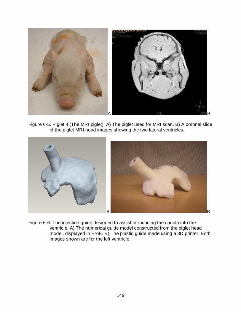
149
A B
Figure 6-5. Piglet 4 (The MRI piglet). A) The piglet used for MRI scan. B) A coronal slice of the piglet MRI head images showing the two lateral ventricles.
A B
Figure 6-6. The injection guide designed to assist introducing the canula into the ventricle. A) The numerical guide model constructed from the piglet head model, displayed in ProE. B) The plastic guide made using a 3D printer. Both images shown are for the left ventricle.

150
Figure 6-7. Post mortem experiment on piglet 4. The EIT system was shown on the back. EEG electrode layout was applied on the piglet scalp using 4mm EEG electrodes. Saline was injected through the top.
Figure 6-8. Difference voltage measurements generated by the two 4ml saline injections on piglet 1.

151
A
B
Figure 6-9. Isosurface plots of reconstructions of injections to the closed skull piglet (piglet 2). A) Injections to the left-hand side. B) Injections to the right-hand side. The three electrodes located together on the equator of the sphere at foreground right of each image are (left to right) electrodes O1, Oz and O2.
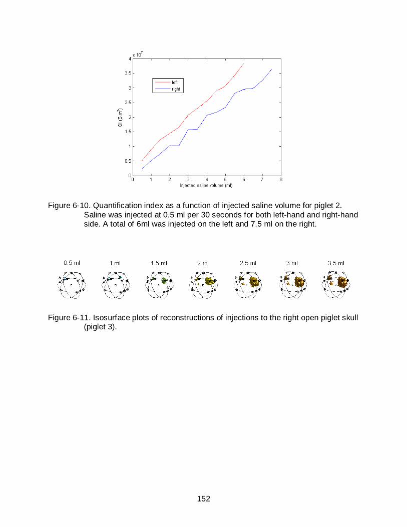
152
Figure 6-10. Quantification index as a function of injected saline volume for piglet 2. Saline was injected at 0.5 ml per 30 seconds for both left-hand and right-hand side. A total of 6ml was injected on the left and 7.5 ml on the right.
Figure 6-11. Isosurface plots of reconstructions of injections to the right open piglet skull (piglet 3).
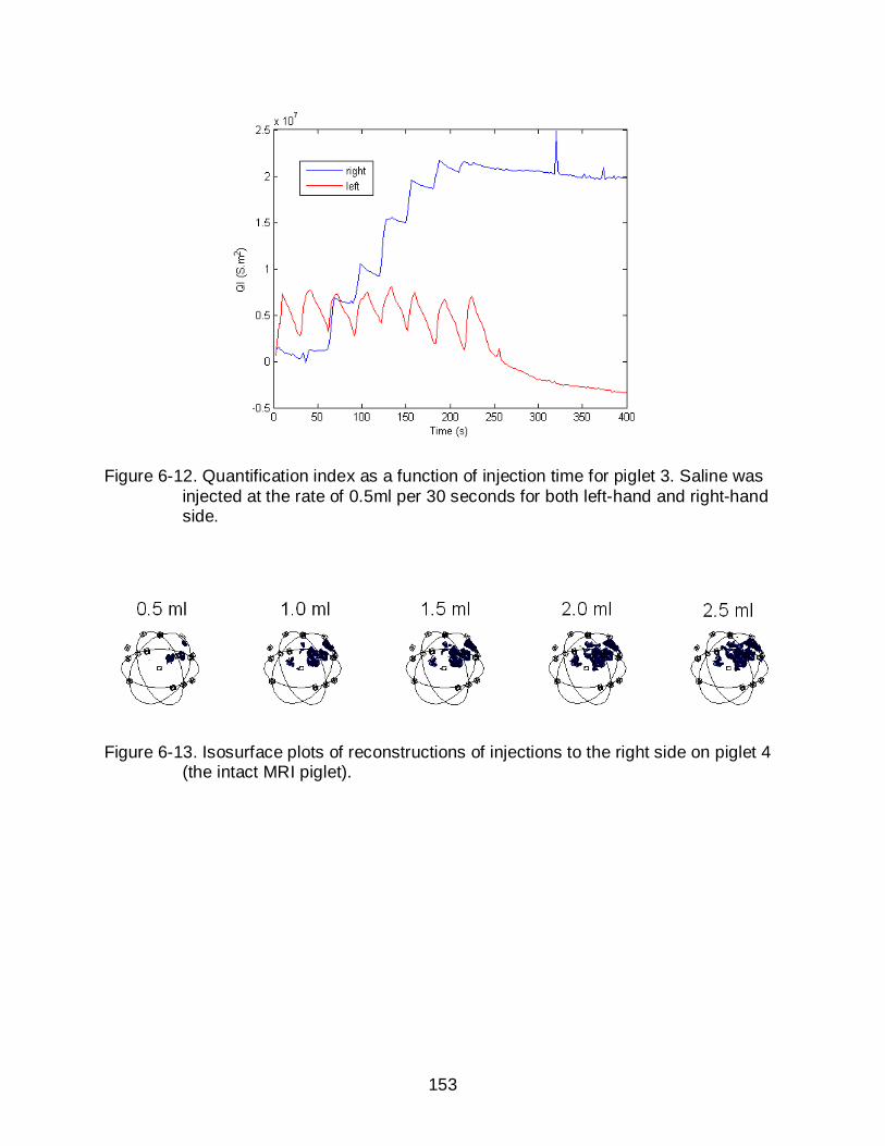
153
Figure 6-12. Quantification index as a function of injection time for piglet 3. Saline was injected at the rate of 0.5ml per 30 seconds for both left-hand and right-hand side.
Figure 6-13. Isosurface plots of reconstructions of injections to the right side on piglet 4 (the intact MRI piglet).

154
A B
Figure 6-14. Quantification index as a function of injection time for piglet 4. A) 0.5 ml injection every 10 seconds on the right side. B) 0.1 ml injection every 10 seconds on the left side.
A B
Figure 6-15. Signals recorded in one of the measurements for piglet 5 and 6. A) Signal changing with time in measurement 79 for piglet 5. B) Signal changing with time in measurement 79 for piglet 6.

155
Figure 6-16. Coronal brain slices of piglet 6. Slice number and thickness are indicated near each slice. The orientations (Superior, Inferior, Left and Right) of all the slices are marked in the figure. The anterior of each slice is facing inside. Blood (indicated with red arrows) can be observed clotted in both ventricles.
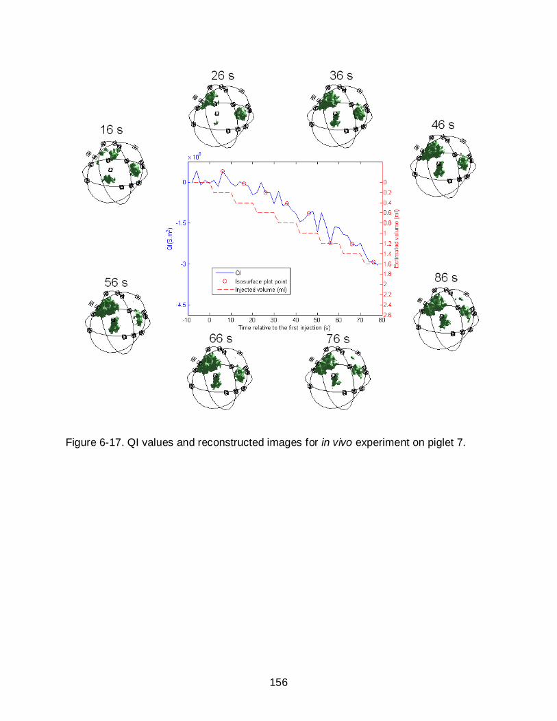
156
Figure 6-17. QI values and reconstructed images for in vivo experiment on piglet 7.

157
Figure 6-18. QI values and reconstructed images for in vivo experiment on piglet 8.
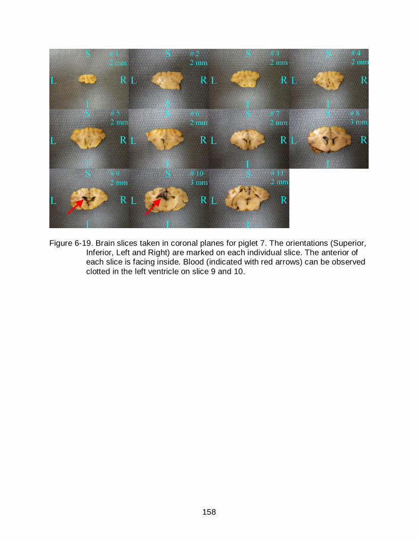
158
Figure 6-19. Brain slices taken in coronal planes for piglet 7. The orientations (Superior, Inferior, Left and Right) are marked on each individual slice. The anterior of each slice is facing inside. Blood (indicated with red arrows) can be observed clotted in the left ventricle on slice 9 and 10.

159
A
B
Figure 6-20. Brain dissection for piglet 8. A) Brain slices taken in coronal planes for piglet 8. The orientations (Superior, Inferior, Left and Right) are marked on each individual slice. The anterior of each slice is facing inside. Blood (indicated with red arrows) can be observed clotted in the left ventricle on slice 6 - 11. B) A cross-sectional coronal plane picture (looking from front) showing the catheter path and blood clotted in the left ventricle. Blood is indicated with a red arrow.
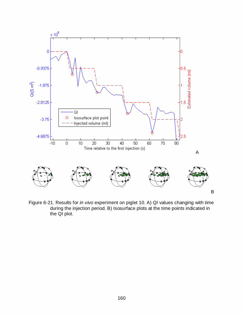
160
A
B
Figure 6-21. Results for in vivo experiment on piglet 10. A) QI values changing with time during the injection period. B) Isosurface plots at the time points indicated in the QI plot.
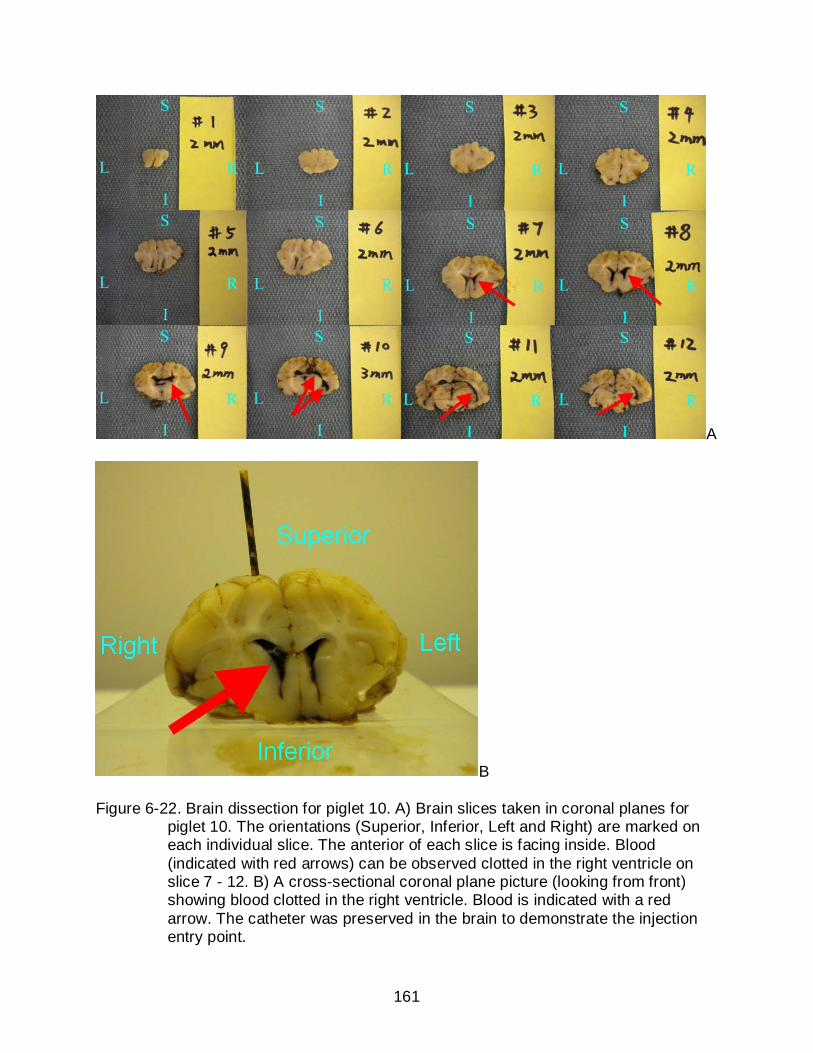
161
A
B
Figure 6-22. Brain dissection for piglet 10. A) Brain slices taken in coronal planes for piglet 10. The orientations (Superior, Inferior, Left and Right) are marked on each individual slice. The anterior of each slice is facing inside. Blood (indicated with red arrows) can be observed clotted in the right ventricle on slice 7 - 12. B) A cross-sectional coronal plane picture (looking from front) showing blood clotted in the right ventricle. Blood is indicated with a red arrow. The catheter was preserved in the brain to demonstrate the injection entry point.
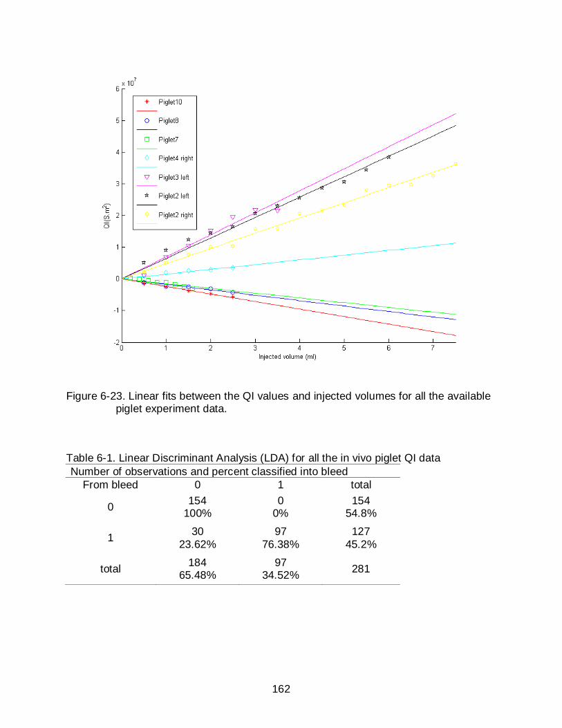
162
Figure 6-23. Linear fits between the QI values and injected volumes for all the available piglet experiment data.
Table 6-1. Linear Discriminant Analysis (LDA) for all the in vivo piglet QI data Number of observations and percent classified into bleed
From bleed 0 1 total
0 154 100%
0 0%
154 54.8%
1 30 23.62%
97 76.38%
127 45.2%
total 184 65.48%
97 34.52% 281

163
CHAPTER 7 SUMMARY
Conclusion
This work aimed to develop an effective method to detect and quantify
intraventricular hemorrhage in premature neonates using Electrical Impedance
Tomography. We started with numerical simulations on a homogeneous spherical head
model, then on a spherical model with important anatomical structures added. Three
candidate current patterns (RING, EEG and Cz-RING patterns) were proposed in the
beginning. After conducting sensitivity analysis, we found that the EEG pattern had the
best sensitivities and selectivities in general in our regions of interest. Reconstructed
images with the EEG pattern using data generated from simulations and saline
phantoms also showed the best image qualities and quantification accuracies. The EEG
pattern could also take advantage of the unique characteristics of a neonatal skull,
which include its higher conductivity and the opening fontanel on top. This was proved
in the sensitivity analysis and the comparison between the open-skull model and
closed-skull model.
The findings from spherical models were then applied on models with realistic
boundary geometries. We studied the effect from model geometry mismatch by
comparing the reconstructions from two sensitivity matrices, one calculated from a
homogeneous spherical model ( SPS ), the other calculated from a realistic geometry
model ( RGS ). The results indicated that the RGS reconstructions guaranteed the best
image qualities only when the subject geometry is perfectly matched with the forward
model. In addition to that, RGS did not show any advantage over S_SP for the purpose
of quantification. Therefore, we concluded that using the spherical sensitivity matrix

164
would be more appropriate for neonate applications, since the head shape varies from
patient to patient.
Piglet animal experiments, both post mortem and in vivo, were conducted to
investigate the true quality of the EEG method. Skull impedances were measured after
each experiment to estimate the radial conductivity for neonatal piglet skulls. We found
that the average conductivity of the fresh skull samples was 27.8 mS/m, which was
about twice higher than the conductivity for adult human skull reported in the literature
(15 mS/m). In post mortem experiments, we injected saline into the piglet brains. We
were able to detect as low as 0.2 ml injections. The QIs showed a stable linear
relationship along with the injections. In the in vivo experiments, we obtained blood from
the piglet’s umbilicus instead of using saline. We successfully injected blood into the
ventricles with the aid of an injection guide. Negative conductivity changes were
observed in the reconstructed images. We also observed a linear relationship between
the QIs and injected blood volumes. The data was more affected by noise compared to
the post mortem experiments data. However, we were able to detect 0.5 ml blood
volumes in two piglets and 0.2 ml blood volumes in one piglet successfully. The QI
scale levels in all the 3 in vivo experiments were consistent. We preserved the piglet
brains for the in vivo experiments and sliced them afterwards. We could observe blood
clotted in the correct side of the ventricles which double confirmed the reconstructed
images. All the promising results indicated that we can use EIT to detect and monitor
intraventricular bleeding in piglets and probably extend this application to premature
neonates.

165
Future Work
Improving in vivo Animal Experiment
We have so far conducted 6 in vivo piglet experiments. More experiments are
needed to validate the reconstruction and quantification standards. Within these 6
experiments, we were able to detect the blood volume in 3 of them, but failed in the
other 3. The failures were presumably caused by bad electrode contacts. It could be
one or multiple of the 16 measurement electrodes or the ground electrode. It would be
very helpful to have a function in the software, so we can check the electrode
connections in real time. The electrodes can also be improved. We have been using
4mm EEG electrodes in the experiments. To attach the electrodes to the scalp, we need
to first put on 16 electrode stickers, and then inject conducting gel into each electrode
carefully and attach them to the stickers. The amount of gel injected into each electrode
needs to be controlled very carefully. Too much or too little will both cause electrode
contact problem. Moreover, this whole process normally took more than half an hour.
However, we should keep in mind that the catheter was already inserted into the brain
when we were working on the electrodes (refer to Appendix B for details). This could
cause physiological changes during a half an hour period and consequently affect our
measurement accuracy. Therefore, new types of electrodes will be appreciated if we
can make this process faster.
Improving the Measurement Strategy
The 16-electrode EEG current pattern has produced promising results in numerical
simulations, phantom experiments and animal experiments. However, this pattern was
not an optimized one. Due to the limitation in hardware design, the measurements were
all taken from adjacent pairs of electrodes. Although it contained all the independent

166
measurements, a number of these measurements were very low in magnitude and were
likely to introduce errors when noise was presented. Our new EPack3 system is an 8-
electrode EIT system. It has more flexibility in selection of current and voltage electrode
pairs. Therefore, we are going to reduce the number of electrodes to 8, and use an
optimized current pattern. Base on our experience from the current work, using 8
electrodes should be enough for the purpose of quantification, although we may have a
compromise in reconstructed image quality. However, using a small number of
electrodes is always desirable in clinical applications since the scalp area of a neonate
is limited. It may also speed up the electrode setup process in the in vivo piglet
experiments .

167
APPENDIX A USEFUL C++ CODE FOR CONJUGATE GRADIENT METHOD
An important subprocess in conjugate gradient optimization is performing line
minimization along each given direction. This involves two procedures, bracketing the
minimum and searching for the minimum within the range. They are implemented in the
following C++ functions: mnbrak() and brent(). The function linmin() calls mnbrak() and
brent(), and accomplish line minimization. The conjugate gradient method is
implemented in frprmn(). For more details, please refer to Press et al. 1989.
Bracket the Minimum
void mnbrak(double *ax,double *bx,double *cx,double *fa,double *fb, double *fc, int n, double *pcom, double *xicom, double *F, double *outarr, double *xt) double ulim,u,r,q,fu,dum; *fa=f1dim(*ax, n, pcom, xicom, F, outarr, xt); *fb=f1dim(*bx, n, pcom, xicom, F, outarr, xt); if (*fb > *fa) SHFT(dum,*ax,*bx,dum) SHFT(dum,*fb,*fa,dum) *cx=(*bx)+GOLD*(*bx-*ax); *fc=f1dim(*cx, n, pcom, xicom, F, outarr, xt); while (*fb > *fc) r=(*bx-*ax)*(*fb-*fc); q=(*bx-*cx)*(*fb-*fa); u=(*bx)-((*bx-*cx)*q-(*bx-*ax)*r)/ (2.0*SIGN(MAX(fabs(q-r),TINY),q-r)); ulim=(*bx)+GLIMIT*(*cx-*bx); if ((*bx-u)*(u-*cx) > 0.0) fu=f1dim(u, n, pcom, xicom, F, outarr, xt); if (fu < *fc) *ax=(*bx); *bx=u; *fa=(*fb); *fb=fu; return; else if (fu > *fb) *cx=u; *fc=fu; return;
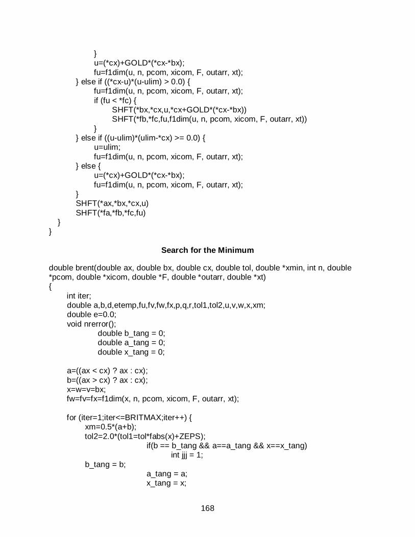
168
u=(*cx)+GOLD*(*cx-*bx); fu=f1dim(u, n, pcom, xicom, F, outarr, xt); else if ((*cx-u)*(u-ulim) > 0.0) fu=f1dim(u, n, pcom, xicom, F, outarr, xt); if (fu < *fc) SHFT(*bx,*cx,u,*cx+GOLD*(*cx-*bx)) SHFT(*fb,*fc,fu,f1dim(u, n, pcom, xicom, F, outarr, xt)) else if ((u-ulim)*(ulim-*cx) >= 0.0) u=ulim; fu=f1dim(u, n, pcom, xicom, F, outarr, xt); else u=(*cx)+GOLD*(*cx-*bx); fu=f1dim(u, n, pcom, xicom, F, outarr, xt); SHFT(*ax,*bx,*cx,u) SHFT(*fa,*fb,*fc,fu)
Search for the Minimum
double brent(double ax, double bx, double cx, double tol, double *xmin, int n, double *pcom, double *xicom, double *F, double *outarr, double *xt) int iter; double a,b,d,etemp,fu,fv,fw,fx,p,q,r,tol1,tol2,u,v,w,x,xm; double e=0.0; void nrerror(); double b_tang = 0; double a_tang = 0; double x_tang = 0; a=((ax < cx) ? ax : cx); b=((ax > cx) ? ax : cx); x=w=v=bx; fw=fv=fx=f1dim(x, n, pcom, xicom, F, outarr, xt); for (iter=1;iter<=BRITMAX;iter++) xm=0.5*(a+b); tol2=2.0*(tol1=tol*fabs(x)+ZEPS); if(b == b_tang && a==a_tang && x==x_tang) int jjj = 1; b_tang = b; a_tang = a; x_tang = x;

169
if (fabs(x-xm) <= (tol2-0.5*(b-a))) *xmin=x; return fx; if (fabs(e) > tol1) r=(x-w)*(fx-fv); q=(x-v)*(fx-fw); p=(x-v)*q-(x-w)*r; q=2.0*(q-r); if (q > 0.0) p = -p; q=fabs(q); etemp=e; e=d; if (fabs(p) >= fabs(0.5*q*etemp) || p <= q*(a-x) || p >= q*(b-x)) d=CGOLD*(e=(x >= xm ? a-x : b-x)); else d=p/q; u=x+d; if (u-a < tol2 || b-u < tol2) d=SIGN(tol1,xm-x); else d=CGOLD*(e=(x >= xm ? a-x : b-x)); u=((fabs(d) >= tol1) ? (x+d) : (x+SIGN(tol1,d))); if(u-x == 0) u = x+0.0001; if(u-x==0) int kkk = 1; fu=f1dim(u, n, pcom, xicom, F, outarr, xt); if (fu <= fx) if (u >= x) a=x; else b=x; SHFT(v,w,x,u) SHFT(fv,fw,fx,fu) else if (u < x) a=u; else b=u;

170
if (fu <= fw || w == x) v=w; w=u; fv=fw; fw=fu; else if (fu <= fv || v == x || v == w) v=u; fv=fu; fprintf(stderr,"Too many iterations in BRENT\n"); *xmin=x; return fx;
Line Minimization
void linmin(double *p,double *xi, int n, double *fret, double *F, double *outarr, double *xt) int j; double xx,xmin,fx,fb,fa,bx,ax; ax=0.0; xx=1.0; bx=2.0; mnbrak(&ax,&xx,&bx,&fa,&fx,&fb, n, p, xi, F, outarr, xt); *fret=brent(ax,xx,bx, LTOL,&xmin, n, p, xi, F, outarr, xt); for (j=0;j<n;j++) xi[j] *= xmin; p[j] += xi[j];
Conjugate Gradient Method
void frprmn(double *p, int n, double ftol, double *F, int proj_ind, double *outarr, double *doutarr, double *xt) double fret; int j,its; double gg,gam,fp,dgg; double *g; double *h; double *xi; g = nvector(n); h = nvector(n); xi = nvector(n);
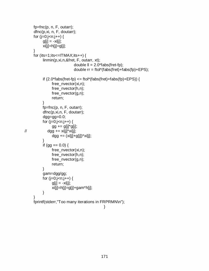
171
fp=fnc(p, n, F, outarr); dfnc(p,xi, n, F, doutarr); for (j=0;j<n;j++) g[j] = -xi[j]; xi[j]=h[j]=g[j]; for (its=1;its<=ITMAX;its++) linmin(p,xi,n,&fret, F, outarr, xt); double ll = 2.0*fabs(fret-fp); double rr = ftol*(fabs(fret)+fabs(fp)+EPS); if (2.0*fabs(fret-fp) <= ftol*(fabs(fret)+fabs(fp)+EPS)) free_nvector(xi,n); free_nvector(h,n); free_nvector(g,n); return; fp=fnc(p, n, F, outarr); dfnc(p,xi,n, F, doutarr); dgg=gg=0.0; for (j=0;j<n;j++) gg += g[j]*g[j]; // dgg += xi[j]*xi[j]; dgg += (xi[j]+g[j])*xi[j]; if (gg == 0.0) free_nvector(xi,n); free_nvector(h,n); free_nvector(g,n); return; gam=dgg/gg; for (j=0;j<n;j++) g[j] = -xi[j]; xi[j]=h[j]=g[j]+gam*h[j]; fprintf(stderr,"Too many iterations in FRPRMN\n");

172
APPENDIX B PROCEDURES FOR IN VIVO PIGLET EXPERIMENTS
• Before experiment starts, use 10U/ml heparin to heparinize all the items that will be in contact with blood, including syringes, needles, catheters and the guide wire.
• Set up the 5% dextrose solution bag (D5 drip) and the administration set with the intravenous pump. Stop the pump at this stage.
• Place the piglet prone on a heated pad.
• Commence isoflurane/O2 administration to the piglet. One person is needed to control the device (watching the reaction from the piglet and adjusting gas pressure). Another person is needed to hold the mask tightly over the piglet snout at all times.
• Remove hair from scalp area using a razor blade. Wetting the hair can make the shaving process easier. Also remove some hair from regions below both ears, where we are going to attach electrodes T7 and T8. Clean the skin with abrasive wipes if necessary. Then dry the skin with paper towel.
• Mark the 16 electrode positions using a permanent (Sharpie) marker.
• Move the piglet into the surgery room and transfer it to the surgery bed.
• Insert the temperature probe into the piglet rectum. Tape the wire onto the piglet tail to hold it firmly.
• Attach oximeter to one rear trotter, and validate readings against heart rate. A person is needed to record the temperature and heart rate every 2 minutes.
• Carefully turn the piglet supine.
• Before doing surgery on the umbilicus, the UVC/UAC needs to be prepared. One end of the catheter has two branches. Connect each of the branches with a 3-way stop cock. One 3-way stop cock is connected with one syringe, which will be used to draw blood from the umbilicus later. The other 3-way stop cock is connected with a syringe and the catheter of the administration set. Both syringes should be filled with some heparin before connecting to the 3-way stop cock. (Figure B-1).
• The surgeon starts working on the umbilicus. A magnifier lamp will be needed to assist finding the blood vessel within the umbilicus. Insert the other end of the UVC/UAC into the vessel. Blood should be seen flowing into the catheter immediately.
• Suture on the UAC/UVC using Addison forceps. Tape down part of the catheter around the umbilicus to make it steady.

173
• Turn the piglet prone carefully. Make sure the UAC/UVC, the temperature probe and the oximeter sensor do not fall off.
• Put the guide (either left or right) on the piglet head. The position can be determined by the ‘eye mark’ and ‘ear mark’ on the guide. Premark the cannula at 17 mm and 66mm with a permanent Sharpie. Introduce the cannula into the guide. Pierce the skull and keep going slowly until the 66mm mark matches the metal attachment in the guide.
• Hold the cannula and take the central needle out slowly. Then raise the guide a little bit and hold the bottom of the cannula, as close to the skin as possible, to make sure the cannula does not move around while taking away the guide. Then remove the guide slowly.
• Introduce the dilator on top of the cannula, slowly. Once the dilator is close to the skin, switch to hold the top of the cannula as quick as possible. Then twist the dilator into the skull nice and easy. Remove the dilator slowly. Once the tip of the dilator is out of skin, switch to hold the bottom of the cannula. Always try your best to hold the cannula in place during this procedure. Bleeding may occur in this process. We may need a person to dip off the bleeding from time to time.
• The hole made by the dilator in the previous step is not big enough to introduce in the 0.08 od catheter. Therefore, we need to use a bigger dilator and repeat the previous procedure.
• Pre-mark the blood injection catheter (0.05 inner diameter, 0.08 outer diameter) at 17 mm. Send in the catheter on top of the cannula the same way we put in the dilators. Twist the catheter into the brain until the mark matches the skin. Once the catheter is in place, remove the cannula slowly.
• (The last 4 procedures have been modified since the experiment on piglet 7 and 8. We first determined the approximate entry point on the skin using the guide. We then cut the skin open and made a hole (diameter approximately 5mm) on the skull using a bone drill. We inserted the cannula following the same procedures. After that, we introduce in the catheter immediately, rather than using the dilator. This new type of polyimide catheter had a much smaller wall thickness and could be inserted without dilating the entry point. We then sutured the skin back in place.)
• Connect a 3 way stop cock with a blunted 16G needle and insert the needle into the other end of the catheter (the needle has to be blunted, otherwise it would pierce the wall when the catheter is bended). Another two ends of the 3 way stop cock are connected with two syringes. One is filled with blood for the blood injection later. The other is empty and haprinized for drawing CSF. Put the ‘stop’ switch to the blood injection syringe, and hold this syringe with a clamp on a stand (Figure B-2).

174
• Put the electrode stickers on the corresponding 16 positions. Then put on the 16 4mm EEG electrode. Electrode gel needs to be injected before putting on each electrode. The amount of gel injected needs to be controlled carefully. If you inject too much, the gel will flow out when pressing the electrode against the sticker. Then you will need to remove that sticker and put a new one there. According to the author’s experience, it will be easier to put on the electrodes on the posterior first, then do the anterior ones. Finally, put an ECG electrode on one of the ears for ground connection. This whole procedure will take approximately 20 minutes.
• Try to remove some CSF using the empty syringe. At least remove the air in the catheter. Then close this branch.
• Turn on the EIT system and start the measurements. First do a complete measurement using their default adjacent ring configuration and make sure there is no voltage over flow. If voltage overflow is observed, we can check the overflow log file and determine which electrode caused the problem, then reconnect that electrode to the skin.
• Start the EEG measurements. Set the scan interval to 2 seconds. Do a baseline measurement for 10 minutes.
• Administrator 0.1 ml blood every 10 seconds, until all the blood is injected.
• Continue recording for another 5 minutes.
• Turn the piglet supine and perform euthanasia.

175
Figure B-1. Experiment picture showing the setups for the umbilicus catheter.
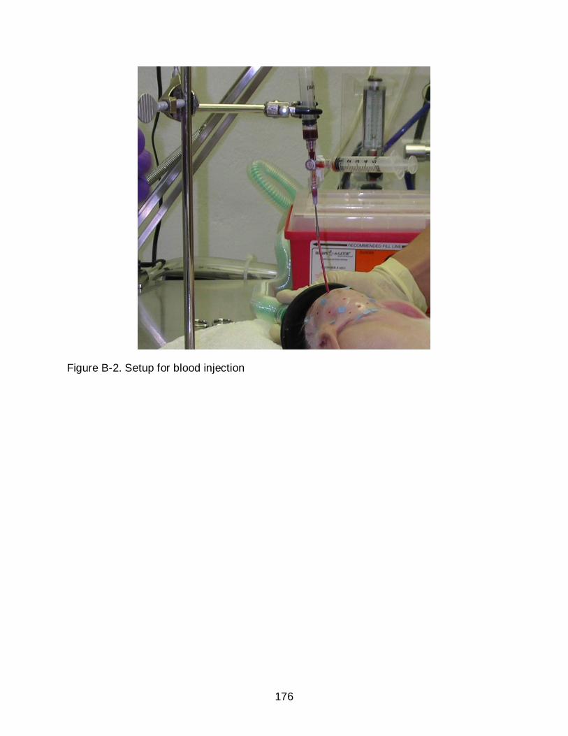
176
Figure B-2. Setup for blood injection

177
LIST OF REFERENCES
Abascal, J P J, Arridge S R, Atkinson D, Horesh R, Fabrizi L, De Lucia M, Horesh L, Bayford R H and Holder D S 2008 Use of anisotropic modeling in electrical impedance tomography; Description of method and preliminary assessment of utility in imaging brain function in the adult human head NeuroImage 43 258-268
Adler A, Arnold J H, Bayford R, Borsic A, Brown B and Dixon P 2009 GREIT: a unified approach to 2D linear EIT reconstruction of lung images Physiological Measurement 30 S35-S55
Aquilina K, Hobbs C, Cherian S, Tucker A, Porter H, Whitelaw A and Thoresen M 2007 A neonatal piglet model of intraventricular hemorrhage and posthemorrhagic ventricular dilation J. Neurosurg. 107(2 Suppl) 126-36
Akkermans L M A and Tekamp F A 1993 The effects of stress on gastric emptying as measured by electrical impedance tomography Clinical and physiological Applications of Electrical Impedance Tomography London: Univ. College London Press, 100-12
Anon 2004 Follow-up care of high-risk infants Pediatrics 114 1377-97
Austin T, Gibson A P, Branco G, Yusof R Md, Arridge S R, Meek J H, Wyatt J S, Delpy D T and Hebden J C 2006 Three dimensional optical imaging of blood volume and oxygenation in the neonatal brain Neuroimage 31 1426-33
Awada K A, Jackson D R, Baumann S B, William J T, Wilton D R, Fink P W and Prasky B R 1998 Effect of conductivity uncertainties and modeling errors on EEG source localization using a 2D model IEEE Trans Biomed. Eng. 45(9) 1135-45
Babcock D S, Bove K E and Han B K 1982 Intracranial hemorrhage in premature infants: sonographi-pathologic correlation Am. J. Neuroradiol. 3 309-17
Bagshaw A P, Liston A D, Bayford R H, Tizzard A, Gibson A P, Tidswell A T, Sparkes M K, Dehghani H, Binnie C D and Holder D S 2003 Electrical impedance tomography of human brain function using reconstruction algorithms based on the finite element method NeuroImage 20 752-764
Baltzell J K, Beser F W, Miguel S G and Borum P R 1987 The neonatal piglet as a model for human neonatal carnitine metabolism J. Nutr. 117 754-757
Barber D C and Brown B H 1984 Applied potential tomography J. Phys. E. Sci. Instrum. 17 723-733
Bayford R H 2006 Bioimpedance Tomography (Electrical Impedance Tomography) Annu. Rev. Biomed. Eng. 8 63-91

178
Bayford R H, Boone K G, Hanquan Y and Holder D S 1996 Improvement of the positional accuracy of EIT images of the head using a Lagrange multiplier reconstruction algorithm with diametric excitation Physiol. Meas. 17 A49-A57
Bertero M and Boccacci P 1998 Introduction to inverse problems in imaging Institute of Physics Publishing, London
Blankenberg F G, Loh N N and Bracci P 2000 Sonography, CT and MR imaging: a prospective comparison of neonates with suspected intracranial ischemia and hemorrhage Am. J. Neuroradiol. 21 213-218
Boone K, Barber D and Brown B 1997 Review: Imaging with electricity: Report of the European concerted action on impedance tomography J. Med. Eng. Tech. 21 201-32
Borsic A, McLeod C, Lionheart W and Kerrouche N 2001 Realistic human thorax modeling for EIT Physiol. Meas. 22 77-83
Brann B S, Wofsy C, Papile L A, Angelus P and Backstrom C 1990 Quantification of neonatal cerebral ventricular volume by real-time ultrasonography J. Ultrasound Med. 9 9-15
Brown B H, Leathard A D, Lu L, Wang W and Hampshire A 1995 Measured and expected Cole parameters from electrical impedance tomographic images of human thorax Physil. Meas. 16 A57-67
Brown B H and Seager A D 1987 The Sheffield data collection system Clin. Phys. Physiol. Meas. 8(Suppl. A) 91-97
Burdjalov V, Srinivasan P, Baumgart S and Spitzer A R 2002 Handheld portable ultrasound in the neonatal intensive care nursery: A new, inexpensive tool for the rapid diagnosis of common neonatal problems Journal of Perinatology 22 478-483
Burger H C and van Milaan J B 1943 Measurement of the specific resistance of the human body to direct current Acta Med. Scand. 114 584–607
Cheney M, Isaacson D, Newell J, Goble J and Simske S 1990 NOSER: An algorithm for solving the inverse conductivity problem Internat. J. Imaging Systems and Technology 2 66-75
Cheney M, Isaacson D and Newell J C 1999 Electrical impedance tomography SIAM Rev. 41(1) 85-101
Cherepenin V A, Karpov A Y, Korjenevsky A V, Kornienko V N and Kultiasov Y S 2002 Three-dimensional EIT imaging of breast tissues: system design and clinical testing IEEE Trans. Med. Imaging 21(6) 662-67

179
Clay M T and Ferree T C 2002 Weighted regularization in electrical impedance tomography with applications to acute cerebral stroke IEEE Trans. Med. Imag. 21 629-637
Cornean H, Knudsen K and Siltanen S 1996 Towards a d-bar reconstruction method for three-dimensional EIT Journal of Inverse and Ill-posed Problems 14 111-134
Epstein B R and Foster K R 1983 Anisotropy in the dielectric properties of skeletal muscle Med. & Biol. Eng. & Comput. 21 51-55
Eyuboglu B M, Brown B H, Barber D C and Seager A D 1987 Localisation of cardiac related impedance changes in the thorax Clin. Phys. Physiol. Meas. 8(A) 167-73
Eyuboglu B M 1996 An interleaved drive electrical impedance tomography image reconstruction algorithm Physiol. Meas. 17(A) 59-71
Faes T J C, van der Meij H A, de Munck J C and Heethaar R M 1999 The electric resistivity of human tissues (100 Hz – 10 MHz): a meta-analysis of review studies Physiol. Meas. 20 R1-10
Fan W, Wang H, Chen X and Lv Z 2009 Three dimensional EIT models for human lung reconstruction based on Schur CG algorithm Complex Medical Engineering CME. ICME International Conference, 1-5
Foster K R and Schwann H P 1989 Dielectric properties of tissues and biological materials: a critical review Crit. Rev. Biomed. Eng. 17(1) 25-104
Gabriel S, Lau R W, and Gabriel C 1996 The dielectric properties of biological tissues: II. Measurements in the frequency range 10Hz to 20 GHz Phys. Med. Biol. 41 2251-2269
Geddes L A and Baker L E 1967 The specific resistance of biological material – a compendium of data for the biomedical engineer and physiologist Med. Biol. Eng. 5 271-293
Geselowitz D B 1971 An application of electrocardiographic lead theory to impedance plethysmography IEEE Trans. Biomed. Eng. 18 38-41
Gibson A, Bayford R H and Holder D S 2000 Two-dimensional finite element modeling of the neonatal head Physiol. Meas. 21 45-52
Gisser D G, Isaacson D and Newell J C 1987 Current topics in impedance imaging Clin. Phys. Physiol. Measurement 8(Suppl. A) 39-46
Gilmore J H, Gerig G, Specter B, Charles H C, Wilber J S, Hertzberg B S and Kliewer M A 2001 Neonatal cerebral ventricle volume: a comparison of 3D ultrasound and magnetic resonance imaging J. Ultrasound Med. 27 1143-6

180
Glickman Y A, Filo O, Nachaliel U, Lenington S, Amin-Spector S and Ginor R 2002 Novel EIS postprocessing algorithm for breast cancer diagnosis IEEE Trans. Med. Imaging 21(6) 710-12
Goldenberg R L and Jobe A H 2001 Prospects for research in reproductive health and birth outcomes JAMA 285 633-9
Gorodnitsky I F and Rao B D 1997 Sparse signal reconstruction from limited data using FOCUSS: A re-weighted minimum norm algorithm IEEE Sig. Proc. 45(3) 600-616
Halter R, Hartov A and Paulsen K D 2004 Design and implementation of a high frequency electrical impedance tomography system Physil. Meas. 25 379-90
Hansen P C 1992 Analysis of discrete ill-posed problems by means of the L-curve SIAM Review 34(4) 561-580
Hansen P C and O’Leary D P 1993 The use of the L-curve in the regularization of discrete ill-posed problems SIAM J. Sci. Comput. 14(6) 1487-1503
Hansen T W R 2006 Prophylaxis of intraventricular hemorrhage in premature infants: New potential tools, new potential challenges Ped. Crit. Care Med. 7 90-92
Helmholtz H L F 1853 Ueber einige Gesetze der Vertheilung elektrischer Ströme in körperlichen Leitern mit Anwendung auf die thierisch-elektrischen Versuche Ann. Physik und Chemie 89 211-33, 354-77
Hintz S R and O’Shea M 2008 Neuroimaging and neurodevelopmental outcomes in preterm infants Sem. Perinatol. 32 11-9
Hoetink A E, Faes T J C, Marcus J T, Kerkkamp H J J and Heethar R M 2002 Imaging of thoracic blood volume changes during the heart cycle with electrical impedance using a liner spot-electrode array IEEE Trans. Med. Imaging 21(6) 653-61
Holdefer R, Sadleir R and Russell M J 2006 Predicted current densities in the brain during transcranial electrical stimulation Clin. Neurophysiol. 117 1388-1397
Holder D S 2005 Electrical Impedance Tomography Methods, History and Applications UK: IOP Publishing
Holder D S and Temple A J 1993 Effectiveness of Sheffield EIT system in distinguishing patients with pulmonary pathology from a series of normal subjects Clinical and Physiological Applications of the Electrical Impedance Tomography. Univ. College London Press
Hua P, Webster J G and Tompkins W J 1987 Effect of the measurement method on noise handling and image quality of EIT imaging In Proc. Ninth Int. Conf. IEEE Eng. In Med. And Biol. Society, IEEE, New York, N.Y. 2 1429-30

181
Huisman T A G M 2005 Intracranial hemorrhage: ultrasound, CT and MRI findings Eur. Radiol. 15 434-440
Hun W and Woo E J 2009 Design of KHU Mark2 Multi-frequency EIT system 10th International Conference on Biomedical Applications of Electrical Impedance Tomography (EIT 2009). University of Manchester, 16th-19th June, 2009
Jones V S, Wood J G, Godfrey C and Cohen R C 2008 An optimum animal model for neonatal thoracoscopy J. Laparoendosc. Adv. Surg. Tech. A. 18(5) 759-62
Kauppinen P, Hyttinen J and Malmivuo J 2005 Sensitivity distribution simulations of impedance tomography electrode combinations IJBEM 7 344-347
Kerner T E, Paulsen K D, Hartov A, Soho S K and Poplack S P 2002 Electrical impedance spectroscopy of the breast: clinical imaging results in 26 subjects IEEE Trans. Med. Imaging 21(6) 638-45
Koksal A and Eyuboglu B M 1995 Determination of optimum injected current patterns in electrical impedance tomography Physiol. Meas. 16(suppl) A99-A109
Lionheart W R B, Kaipio J and McLeod C N 2001 Generalized optimal current patterns and electrical safety in EIT Physiol. Meas. 22 85-90
Liston A D, Bayford R H, Tidswell A T and Holder D S 2002 A multi-shell algorithm to reconstruct EIT images of brain function Physiol. Meas. 23 105-119
Liston A D, Bayford R H and Holder D S 2004 The effect of layers in imaging brain function using electrical impedance tomography Physiol. Meas. 25 143-158
Liu N, Saulnier G, Newell J C and Kao T 2005 ACT4: a high-precision, multi-frequency electrical impedance tomography Conf. Biomed. Appl. Elec. Impedance Tomography. University College London. 22-24th June, 2005
Liu P and Griffiths H 1993 Limitations to sensitivity of EIT in monitoring tissue temperature in hyperthermia Clinical and physiological Applications of Electrical Impedance Tomography, London: Univ. College London Press, 211-17
Ljaz U Z, Khambampati A K, Lee J S, Kim S and Kim K Y 2008 Nonstationary phase boundary estimation in electrical impedance tomography using unscented Kalman filter J. of Comput. Phys. 277(15) 7089-7112
Mack L A, Wright K, Hirsch J H, Alvord E C, Guthrie R D, Shuman W P, Rogers J V and Bolender N F 1981 Intracranial hemorrhage in premature infants: accuracy of sonographic evaluation Am. J. Roentgenol. 137 245-50
Malmivuo J and Plonsey R 1995 Bioelectromagnetism New York

182
Mangnall Y F, Baxter A J, Avill R, Bird N C and Brown B H 1987 Applied potential tomography: a new non-invasive technique for assessing gastric function Clin. Phys. Physiol. Meas. 8(A) 119-31
Mangnall Y F, Kerrigan D D, Johnson A G and Read N W 1991 Applied potential tomography: Noninvasive method for measuring gastric emptying of a solid test meal Dig. Dis. Sci. 36(12) 1680-1684
McArdel F J, Brown B H, Pearse R G and Barber D C 1988 The effect of the skull of low-birth weight neonates on applied potential tomography imaging of centralized resistivity changes Clin. Phys. Physiol. Meas. 9A 55-60
McInerney T and Terzopoulos D 1996 Deformable models in medical image analysis: A survey Medical Image Analysis, 1(2) 91-108
Meeson S, Killingback A L T and Blott B H 1995 The dependence of EIT images on the assumed initial conductivity distribution: a study of pelvic imaging Phys. Med. Biol. 40 643-657
Ment L R, Bada H S, Barnes P, Grant P E, Hirtz D, Papile L A, Pinto-Martin J and Slovis T L 2002 Practice parameter: neuroimaging of the neonate – report of the quality standards subcommittee of the American academy of neurology and the practice committee of the child neurology society Neurology 58 1726-38
Ment L R 1994 Low-dose indomethacin and prevention of intraventricular hemorrhage: a multicenter randomized trial Pediatrics 93 543-50
Metherall P, Barber D C, Smallwood R H and Brown B H 1996 Three dimensional electrical impedance tomography Nature 380 509-512
Moskowitz M J, Ryan T P, Paulsen K D and Mitchell S E 1995 Clinical implementation of electrical impedance tomography with hyperthermia Intl. J. Hyperthermia 11(2) 141-149
Mueller J L, Isaacson D and Newell J C 2001 Reconstruction of conductivity changes due to ventilation and perfusion from EIT data collected on a rectangular electrode array Physiol. Meas. 22(1) 97-107
Murai T and Kagawa Y 1985 Electrical Impedance Computed Tomography Based on a Finite Element Model IEEE Trans. Biomed. Engr. BME32 177-184
Murphy D, Burton P, Coombs R, Tarassenko L and Rolfe P 1987 Impedance imaging in the newborn Clin. Phys. Physiol. Meas. 8A 131-40
Murrieta-Lee J C, Pomfrett C J D, Beatty P C W, Polydorides N, Mussel D B, Waterfall R C and McCann H 2004 Sub-second observations of EIT voltages changes on the human scalp due to brain stimulus Proc. 26th Annual International Conf. on the IEEE EMBS, San Francisco, CA, USA, September, 1-5

183
Nachman A I 1996 Global uniqueness for a two-dimensional inverse boundary value problem Annals of Mathematics 143 71-96
Ni A, Dong X, Yang G, Fu F and Zhu X 2006 Using a priori information to improve on localization of conductivity changes in brain in electrical impedance tomography IFMBE Proc. World Congress on Medical Physics and Biomedical Engineering 2006
Nour S, Mangnall Y F and Dickson A S 1995 Applied potential tomography in the measurement of gastric empting in infants J. Ped. Gast. Nutr. 20 65-72
Oh S 2009 Compensation of shape change artifacts and spatially-variant image reconstruction problems in electrical impedance tomography PhD thesis. University of Florida, USA.
Oh S, Tang T, Tucker A S and Sadleir R J 2009 Normalization of a spatially variant image reconstruction problem in electrical impedance tomography using system blurring properties Physiol. Meas. 30 275-289
Oh T I, Woo E J and Holder D 2007a Multi-frequency EIT system with radially symmetric architecture: KHU Mark1 Physiol. Meas. 28 S183-96
Oh T I, Lee K H, Kim S M, Koo W, Woo E J and Holder D 2007b Calibration methods for a multi-channel multi-frequency EIT system Physiol. Meas. 28 1175-88
Oh T I, Koo W, Lee K H, Kim S M, Lee J, Kim S W, Seo J K and Woo E J 2008 Valication of a multi-frequency electrical impedance tomography (mfEIT) system KHU Mark1: impedance spectroscopy and time-difference imaging Physiol. Meas. 29 295-307
Oostendorp T, Delbeke J and Stegeman D 2000 The conductivity of the human skull: results of in vivo and in vitro measurements IEEE Trans. Biomed. Engr. 47 1487-1492
Papile L A, Burstein J, Burstein R and Koffler H 1978 Incidence and evolution of subependymal and intraventricular hemorrhage: A study of infants with birth weights less than 1500 gm J. Pediatrics. 92 529-534
Pidcock M K, Kuzuoglu M and Leblebicioglu K 1995a Analytic and semi-analytic solutions in electrical impedance tomography: I. Two-dimensional problems Physiol. Meas. 16 77-90
Pidcock M K, Kuzuoglu M and Leblebicioglu K 1995b Analytic and semi-analytic solutions in electrical impedance tomography: II. Three-dimensional problems Physiol. Meas. 16 91-110
Pohlmeier R, Buchner H, Knoll A, Beckmann R and Pesh J 1997 The influence of skull – conductivity misspecification on inverse source localization in realistically shaped finite element models Brain Topogr. 9 157-162

184
Press W H, Flannery B P, Teukolsky S A and Vetterling W T 1989 Numerical Recipes in Pascal Published by the Press Syndicate of the University of Cambridge
Puiman P and Stoll B 2008 Animal models to study neonatal nutrition in humans Current Opinion in Clinical Nutrition and Metabolic Care 11 601-606
Rahim R A, Huei L Y, San C K, Fea P J and Lean L C 2003 Initial result on electrical impedance tomography Jurnal Teknologi. 39(D) 105-113
Rao A. Gibson A and Holder D S 1997 EIT images of electrically induced epileptic activity in anaesthetized rabbits Med. Biol. Eng. Comput. 35(1) 327
Romsauerova A, McEwan A, Horesh L, Yerworth R, Bayford R H and Holder D S 2006 Multi-frequency electrical impedance tomography (EIT) of the adult human head: initial findings in brain tumours, arteriovenous malformations and chronic stroke, development of an analysis method and calibration Physiol. Meas. 27 S147-S161
Ross A S 2003 An adaptive current tomography for breast cancer detection PhD Thesis Rensselaer Polytechnic Institute, Troy, NY, USA
Sadleir R J and Fox R A 1998 Quantification of blood volume by Electrical Impedance Tomography using a tissue equivalent phantom Physiol. Meas. 19 501-516
Sadleir R J and Fox R A 2001 Detection and quantification of intraperitoneal fluid using electrical impedance tomography IEEE Trans. Biomed. Eng. 48 484-91
Sadleir R and Argibay A 2006 Skull impedance measurements in preserved tissue and neonatal piglet 7th Conference on Biomedical Applications of Electrical Impedance Tomography, 27-31 September 2006 pp 111
Sadleir R J, Zhang S U, Tucker A S and Oh S 2008a Imaging and quantification of anomaly volume using an eight electrode ‘hemiarray’ EIT reconstruction method Physiological Measurement. 29 913-927
Sadleir R J, Tucker A S, Oh S and Tang T 2008b Portable eight-electrode EIT system for detection and quantification of abdominal hemorrhage Proceedings EIT conference 2008, Dartmouth College, Hanover, 16th-18th June, 2008 pp 150-154
Sadleir R J, Tucker A S, Oh S and Tang T 2008c Use of an eight-electrode hemiarray EIT electrode configuration for in-vivo fluid quantification Proceedings EIT conference 2008, Dartmouth College, Hanover, 16th-18th June, 2008 pp 118-121
Sadleir R J and Tang T 2009 Electrode configurations for detection of intraventricular haemorrhage in the premature neonate Physiol. Meas. 30 63-79
Sadleir R J, Neralwala F, Tucker A S and Tang T 2009 A controllably anisotropic conductivity or diffusion phantom constructed from isotropic layers Ann. Biomed. Eng. 37(12) 2522-31

185
Santosa F and Vogelius M 1990 A back projection algorithm for electrical impedance imaging SIAM. J. APPL. MATH. 50 216-243
Schierlitz L, Huppi P S, Jakab M, Kikinis R, Frates M C, Mc Tempany C and Jolesz F A 2001 Three-dimensional modeling and volume assessment of the fetal and neonatal intracranial ventricles Proc. Intl. Soc. Mag. Reson. Med. 9
Seagar A D, Barber D C and Brown B H 1987 Theoretical limites to sensitivity and resolution in impedance imaging Clin. Phys. Physiol. Meas. 8 Suppl. A 13-31
Siltanen S, Mueller J L and Isaacson D 2000 An implementation of the reconstruction algorithm of A. Nachman for the 2-D inverse conductivity problem Inverse Problems 16 681-99
Smith R W M, Brown B H, Freeston I L, McArdle F J and Barber D C 1990 Real time electrical impedance imaging. Proc 12th. Ann Conf. of IEEE EMBS, 104-105
Somersalo E, Cheney M and Isaacson D 1991 Layer stripping: a direct numerical method for impedance imaging Inv. Prob. 7 899-926
Stephanesco S and Schlumberger C 1930 Sur la distribution electric autour d’une prise de tere ponctuelle dans un terrain a couches horizontals, homogenes et istotropes F. Phys. Radium Sen. 7 132-40
Stoy R D, Foster K R and Schwan H P 1982 Dielectric properties of mammalian tissues from 0.1 to 100 MHz: A summary of recent data Phys. Med. Biol. 27 501–514
Tang T, Oh S and Sadleir R J 2010 A robust current pattern for the detection of intraventricular hemorrhage in neonates using electrical impedance tomography Ann Biomed Eng. 38(8) 2733-47
Tidswell A T, Gibson A, Bayford R H and Holder D S 2001a Three dimensional electrical impedance tomography of human brain activity NeuroImage 13 283-294
Tidswell A T, Gibson A, Bayford R H and Holder D S 2001b Electrical impedance tomography of human brain activity with a two-dimensional ring of scalp electrodes Physiol. Meas. 22 167-175
Tidswell A T, Gibson A, Bayford R H and Holder D S 2001c Validation of a 3D reconstruction algorithm for EIT of human brain function in a realistic head-shaped tank Physiol. Meas. 22 177-185
Tizzard A, Horesh L, Yerworth R J, Holder D S and Bayford R H 2005 Generating accurate finite element meshes for the forward model of the human head in EIT Physiol. Meas. 26 S251-S261

186
von Ellenrieder N, Muravchik C H and Nehorai A 2006 Effects of geometric head model perturbations on the EEG forward and inverse problems IEEE Trans. Biomed. Engr. 53 421-429
Walker G C, Berry E, Smye S W and Brettle D S 2004 Materials for phantoms for terahertz pulsed imaging Med. Biol. 49 N363-9
Webster J G 1990 Electrical Impedance Tomography UK: IOP Publishing
Wilson A J, Milnes P, Waterworth A R, Smallwood R H and Brown B H 2001 Mk3.5: a modular, multi-frequency successor to the Mk3a EIS/EIT system Physiol. Meas. 22 49-54
Wort P, Church P, and Gagnon S 1999 Preliminary assessment of electrical impedance tomography technology to detect mine-like objects Proceedings of SPIE, the International Society for Optical Engineering 3710(2) 895-905
Xu C, Dong X, Fu F, Shuai W, Liu X and Zhang C 2007 A novel image monitoring software system of electrical impedance tomography for internal hemorrhage IFMBE Proc. World Congress on Medical Physics and Biomedical Engineering 2006 14 3882-3885
Xu P 1998 Truncated SVD methods for discrete linear ill-posed problems Geophys. J. Int. 135 505-514
Yang F and Patterson R P 2008 A simulation study on the effect of thoracic conductivity inhomogeneities on sensitivity distributions Ann. Biomed. Eng. 36 762-8
Yerworth R J, Bayford R H, Cusick G, Conway M and Holder D S 2002 Design and performance of the UCLH Mark 1b 64 channel electrical impedance tomography (EIT) system, optimized for imaging brain function Physiol. Meas. 23(No. 1) 149-58
York J and DeVoe M 2002 Health Issues in Survivors of Prematurity Southern Medical Journal. 95 969-976
Yorkey T, Webster J and Tompkins W 1987 Comparing reconstruction algorithms for electrical impedance tomography IEEE Trans. Biomedical Eng. BME-34 843-852
You F, Shuai W, Shi X, Fu F, Liu R and Dong X 2008 Monitoring retroperitoneal bleeding model of piglets by electrical impedance tomography 30th Annual International IEEE EMBS Conference, Vancouver, British Columbia, Canada, August, 20-24
Yue X and McLeod C 2008 FPGA design and implementation for EIT data acquisition Physiol. Meas. 29 1233-1246
Yvert B, Bertrand O, Thvenet M, Echallier J F and Pernier J 1997 A systematic evaluation of the spherical model accuracy in EEG dipole localization Electroencephalogr. Clin. Neurophysiol. 102 452-459

187
Zhu Q, Lionheart W R B, Lidgey F J, McLeod C N, Paulson K S and Pidcock M K 1993 An adaptive current tomography using voltage sources IEEE Transactions on Biomedical Engineering. 40(2) 163-8
Zhu Q, McLeod C N, Denyer C W, Lidgey F J and Lionheart W R B 1994 Development of a real-time adaptive current tomography Physiol. Meas. 15 A37-43

188
BIOGRAPHICAL SKETCH
Te Tang was born in 1982 in Daqing, China. He graduated from the Daqing high
school and entered the Tsinghua University in the year 1999. He earned his bachelor’s
degree in 2003 in Biomedical Engineering. In the same year, he started to work in the
Tsinghua Tongfang Co. Ltd. in Beijing as a fulltime programmer, expertise in Visual
C++. In the year 2005, he moved to the USA and began his PhD study in biomedical
engineering at the University of Florida.