detection of histological features in liver biopsy …

DETECTION OF HISTOLOGICAL FEATURES IN LIVER BIOPSY

IMAGES TO HELP IDENTIFY NON-ALCOHOLIC FATTY LIVER

DISEASE

by

Deepak Sethunath

A Thesis

Submitted to the Faculty of Purdue University

In Partial Fulfillment of the Requirements for the degree of

Master of Science

Department of Computer and Information Sciences

Indianapolis, Indiana

May 2018

ii

THE PURDUE UNIVERSITY GRADUATE SCHOOL

STATEMENT OF COMMITTEE APPROVAL

Dr. Mihran Tuceryan, Chair


Dr. Shiaofen Fang


Dr. Jiang-Yu Zheng


Approved by:

Dr. Mihran Tuceryan

Head of the Graduate Program

iii

This research is dedicated to my family and friends

iv

ACKNOWLEDGMENTS

I would like to take this opportunity to thank Dr. Mihran Tuceryan, my faculty advisor for

his constant support and guidance throughout my time here at Indiana University Purdue

University, Indianapolis (IUPUI). I believe that he is one of the nicest and humble persons to come

across and it would not have been possible for me to have completed this research without his day

to day help.

I would also like to thank Dr. Jiang Yu Zheng and Dr. Shiaofen Fang for agreeing to be a

part of my Thesis committee. It’s an honor for me indeed. In general, I would like to thank the

entire staff of the Department of Computer Science here at IUPUI who have taught me various

computer science related courses which has extensively helped me in this study.

I am particularly grateful for the assistance and direction given by Dr. Samer Gawrieh, who

has always encouraged me at all the stages of this thesis. He is indeed one of the most encouraging

persons I have met in a long time. I express my sincere gratitude to Dr. David E Kleiner and Dr.

Oscar W Cummings for providing me with their technical expertise in the field of Pathology and

Medicine, required for this study.

I would like to offer my sincere thanks to all my roommates for bearing through all my

tantrums at home and helping me out with their knowledge, as and when needed. Finally, I wish

to thank my family for their constant support and encouragement throughout my study.

v

TABLE OF CONTENTS

LIST OF TABLES ........................................................................................................................ vii

LIST OF FIGURES ..................................................................................................................... viii

ABSTRACT ................................................................................................................................... xi

1. INTRODUCTION ................................................................................................................... 1

Motivation ........................................................................................................................... 1

Problem Statement .............................................................................................................. 2

Contributions of this thesis ................................................................................................. 2

2. BACKGROUND ..................................................................................................................... 5

Liver Anatomy .................................................................................................................... 5

Liver Biopsy........................................................................................................................ 6

Histological Features of Non Alcoholic Fatty Liver Disease ............................................. 8

Previous Work .................................................................................................................. 10

2.4.1 Steatosis ..................................................................................................................... 10

2.4.2 Inflammation .............................................................................................................. 11

2.4.3 Fibrosis ...................................................................................................................... 12

3. METHODOLOGY ................................................................................................................ 14

Types of Biopsy Data Used .............................................................................................. 16

Image Data ........................................................................................................................ 19

Pathologist Grades and Annotations ................................................................................. 20

3.3.1 Annotation Tool ......................................................................................................... 20

Steatosis Classification ..................................................................................................... 29

3.4.1 Macro Fat Detection .................................................................................................. 29

3.4.2 Micro Fat Detection ................................................................................................... 31

3.4.3 Feature Vector representation .................................................................................... 33

3.4.4 External Validation of Classifier’s Accuracy ............................................................ 34

3.4.5 Quantification of Macro Fat ...................................................................................... 35

Inflammation Classification .............................................................................................. 35

3.5.1 Lobular and Portal Inflammation Detection .............................................................. 35

3.5.2 External Validation of Classifier’s accuracy ............................................................. 37

vi

3.5.3 Quantification of Inflammation ................................................................................. 37

Fibrosis Classification ....................................................................................................... 37

3.6.1 Blue region Extraction ............................................................................................... 40

3.6.2 Attribute vector representation .................................................................................. 41

3.6.3 Different types of Fibrosis Detection ........................................................................ 43

3.6.4 Quantification of Collagen ........................................................................................ 44

4. RESULTS .............................................................................................................................. 45

Validation Metrics ............................................................................................................ 45

Steatosis ............................................................................................................................ 48

Lobular and Portal Inflammation ...................................................................................... 54

Fibrosis .............................................................................................................................. 59

5. DISCUSSION ........................................................................................................................ 69

6. CONCLUSION...................................................................................................................... 70

REFERENCES ............................................................................................................................. 71

vii

LIST OF TABLES

Table 3-1 : The different types of annotations present in the web annotation tool. ..................... 22

Table 3-2 : The number of NAFLD lesion annotations present for mice liver biopsies. ............. 24

Table 3-3 : The number of lesion annotations present for human liver biopsies. ......................... 24

Table 3-4 : The different anatomical structures present in a liver biopsy. ................................... 25

Table 3-5 : The number of annotations present for mice liver biopsies. ...................................... 25

Table 3-6 : The number of annotations present for human liver biopsies. ................................... 26

Table 3-7 : The different types of control tissues. ........................................................................ 26

Table 3-8 : The number of annotations present for mice liver biopsies. ...................................... 26

Table 3-9 : The number of annotations present for human liver biopsies. ................................... 27

Table 3-10 : A few histological areas incorporated while taking a liver biopsy. ......................... 27

Table 3-11 : The number of annotations present for mice liver biopsies. .................................... 28

Table 3-12 : The number of annotations present for human liver biopsies. ................................. 28

Table 3-13 : Cumulative number of annotations available on mice and human. ......................... 29

Table 4-1 : Confusion matrix of order 2. ...................................................................................... 45

Table 4-2 : The confusion matrix and metrics for the model built to detect macrosteatosis. ....... 50

Table 4-3 : The confusion matrix and metrics for the model built to detect microsteatosis. ........ 50

Table 4-4 : The confusion matrix and metrics for the model built to detect inflammation. ......... 56

Table 4-5 : The confusion matrix for the model built to detect Normal Fibrosis. ........................ 63

Table 4-6 : The confusion matrix for the model built to detect Pericellular Fibrosis. .................. 64

Table 4-7 : The confusion matrix for the model built to detect Portal Fibrosis............................ 65

Table 4-8 : The confusion matrix for the model built to detect Periportal Fibrosis. .................... 65

Table 4-9 : The confusion matrix for the model built to detect Bridging Fibrosis. ...................... 66

Table 4-10 : The confusion matrix for the model built to detect Nodule Fibrosis. ...................... 67

Table 4-11 : The different types of fibrosis detection with their respective precisions. ............... 68

viii

LIST OF FIGURES

Figure 2-1 : Portal Triad – regions of connective tissue which include branches of bile duct,

portal vein and hepatic artery (13). ........................................................................... 5

Figure 2-2 : An example of a liver biopsy. A. H&E Stain image B. TC Stain image .................... 7

Figure 3-1 : The flow diagram presenting the overall approach. .................................................. 15

Figure 3-2 : Representative Hematoxylin and Eosin images of different models used to

induce fatty liver. A. Normal liver in wild type mouse fed chow diet. B. Mild

fatty liver in wild type mouse fed high fat diet. C. Moderate fatty liver in GFP-

LC3 mouse fed alcohol. D. Severe fatty liver in GFP-LC3 mouse fed high-fat

high-carbohydrate diet. ............................................................................................ 17

Figure 3-3 : Pictorial representation of number of mice liver biopsies graded by Dr. C.............. 18

Figure 3-4 : Pictorial representation of number of human liver biopsies graded by Dr. K. ......... 19

Figure 3-5 : Pictorial representation of number of human liver biopsies graded by Dr. C. ......... 19

Figure 3-6 : A Preview of the mice liver labeling tool with point and boundary annotations

labeled at 6x magnification. .................................................................................... 23

Figure 3-7 : A Preview of the human liver labeling tool with square annotations (fibrosis

annotations) labeled at 6x magnification................................................................. 23

Figure 3-8 : White regions in mouse liver biopsy......................................................................... 29

Figure 3-9 : Overall flow diagram of the approach to automated macrosteatosis identification

and quantification. ................................................................................................... 31

Figure 3-10 : Graphic showing dark and white regions with point and polygon annotations.

The white region labeled using point annotation (represented using 'X') is used

for extracting attributes. A polygon annotation is shown using black polygon.

The white regions falling within the polygon are indicated by arrows and these

are the regions used for attribute extraction for the given label. ............................. 31

Figure 3-11 : Overall flow diagram of the approach to automated microsteatosis

identification. ........................................................................................................... 33

Figure 3-12 : The different dark regions present in a liver biopsy slide. ...................................... 36

ix

Figure 3-13 : Different types of fibrosis annotated. A. Normal Fibrosis B. Pericellular

Fibrosis C. Portal Fibrosis D. Periportal Fibrosis E. Bridging Fibrosis F.

Nodule. .................................................................................................................... 39

Figure 3-14 : The figure shows the pictorial representation of the steps involved in extracting

the collagen in a liver biopsy. .................................................................................. 41

Figure 4-1 : A scatter plot showing correlation between model-computed percentage steatosis

for mouse biopsies with respect to the corresponding pathologist grade. ............... 51

Figure 4-2 : Mixed line/bar chart showing the correlation between the computed percentage

steatosis with the expert pathologist grade. The pathologist grade for mouse

samples is shown as a bar matching the left axis, and the computed percentage

steatosis is shown as a line matching the right axis. ............................................... 51

Figure 4-3 : A graph which represents the different steatosis models generated and their

respective metrics. ................................................................................................... 52

Figure 4-4 : Comparison of annotated macrosteatosis lesions by Pathologist v/s our model.

The left slide contains annotations given by the pathologist (marked as a point

in magenta). The right slide contains macro fat lesions detected by the model

(marked as point in dark blue). ................................................................................ 53

Figure 4-5 : Comparison of annotated microsteatosis lesions by Pathologist v/s our model.

The left slide contains annotations given by the pathologist (marked as

polygons in dark blue). The right slide contains micro fat lesions detected by

the model (marked as polygons in green). .............................................................. 53

Figure 4-6 : Some misclassified instances of microsteatosis lesions. The left slide contains no

micro fat according to the pathologist. The right slide contains wrongly

classified micro fat lesions detected by the model (marked as polygons in

green). ...................................................................................................................... 54

Figure 4-7 : A graph which represents the different inflammation models generated and their

respective metrics. ................................................................................................... 55

Figure 4-8 : A scatter plot showing correlation between model-computed percentage portal

inflammation for human biopsies with respect to the corresponding Dr K’s

grade. ....................................................................................................................... 56

x

Figure 4-9 : A scatter plot showing correlation between model-computed percentage lobular

inflammation for human biopsies with respect to the corresponding Dr K’s

grade. ....................................................................................................................... 57


inflammation for human biopsies with respect to the corresponding Dr C’s

grade. ....................................................................................................................... 57


inflammation for human biopsies with respect to the corresponding Dr C’s

grade. ....................................................................................................................... 58


inflammation for human biopsies with respect to the average of Dr C and Dr

K’s pathologist grade. ............................................................................................. 58


inflammation for human biopsies with respect to the average of Dr C and Dr

K’s pathologist grade. ............................................................................................. 59

Figure 4-14 : An example of blue region detection in a TC Stained sub-slide. A) A TC

Stained sub-slide. B) Blue regions in the TC Stained sub-slide. ............................. 60

Figure 4-15 : A scatter plot showing correlation between model-computed percentage

collagen content for human biopsies with respect to the Dr K’s pathologist

grade. ....................................................................................................................... 61

Figure 4-16 : A scatter plot showing correlation between model-computed percentage

collagen content for human biopsies with respect to the Dr C’s pathologist

grade. ....................................................................................................................... 62

Figure 4-17 : A bar graph which shows semi-quantitative grades given by both Dr. K and

Dr. C for the given test set of 17 human liver slides. .............................................. 62

xi

ABSTRACT

Author: Sethunath, Deepak. MS

Institution: Purdue University

Degree Received: May 2018

Title: Detection of Histological Features in Liver Biopsy Images to Help Identify Non-Alcoholic

Fatty Liver Disease.

Major Professor: Mihran Tuceryan

This thesis explores a minimally invasive approach of diagnosing Non-Alcoholic Fatty Liver

Disease (NAFLD) on mice and humans which can be useful for pathologists while performing

their diagnosis. NAFLD is a spectrum of diseases going from least severe to most severe – steatosis,

steatohepatitis, fibrosis and finally cirrhosis. This disease primarily results from fat deposition in

the liver which is unrelated to alcohol or viral causes. In general, it affects individuals having a

combination of at least three of the five metabolic syndromes namely, obesity, hypertension,

diabetes, hypertriglyceridemia, and hyperlipidemia. Given how common these metabolic

syndromes have become, the rate of NAFLD has increased dramatically over the years affecting

about three-quarters of all obese individuals including many children, making it one of the most

common diseases in United States. Our study focuses on building various computational models

which help identify different histological features in a liver biopsy image, thereby analyzing if a

person is affected by NAFLD or not. Here, we develop and validate the performance of automated

classifiers built using image processing and machine learning methods for detection of macro- and

microsteatosis, lobular and portal inflammation and also categorize different types fibrosis in

murine and human fatty liver disease and study the correlation of automated quantification of

macrosteatosis, lobular and portal inflammation, and fibrosis (amount of collagen) with expert

pathologist’s semi-quantitative grades. Our research for macrosteatosis and microsteatosis

prediction shows the model’s precision and sensitivity as 94.2%, 95% for macrosteatosis and

79.2%, 77% for microsteatosis. Our models detect lobular and portal inflammation(s) with a

precision, sensitivity of 79.6%, 77.1% for lobular inflammation and 86%, 90.4% for portal

inflammation. We also present the first study on identification of the six different types of fibrosis

having a precision of 85.6% for normal fibrosis and >70% for portal fibrosis, periportal fibrosis,

pericellular fibrosis, bridging fibrosis and cirrhosis. We have also quantified the amount of

collagen in a liver biopsy and compared it to the pathologist semi-quantitative fibrosis grade.

1

1. INTRODUCTION

This thesis involves building classifiers to detect different histological features in a liver

biopsy image which in turn will help in the identification of non-alcoholic fatty liver disease

(NAFLD). This is a novel approach of detecting NAFLD, predominantly because we not only

identify steatosis or inflammation in liver but also classify different types of fibrosis, and quantify

the amount of fibrosis.

Motivation

Medical technology is imperative for the betterment of people’s health and well-being. It

also contributes billions of dollars to the economy. Innovative technology is a perquisite to

healthcare.

NAFLD is subdivided into nonalcoholic fatty liver (NAFL) and nonalcoholic

steatohepatitis (NASH) although these are considered to be part of a spectrum. In NAFL, hepatic

steatosis is present without evidence of hepatocyte ballooning degeneration or significant

inflammation, whereas in NASH, hepatic steatosis is associated with hepatocyte ballooning

degeneration and hepatic inflammation that may be histologically indistinguishable from alcoholic

steatohepatitis (1).

According to Younossi et al. NAFLD is one of the most important causes of liver disease

worldwide in adults and children due to the pandemic spread of obesity. “Global prevalence of

NAFLD is estimated at 24%; the highest rates are reported from South America and the Middle

East, followed by Asia, the USA and Europe. The large volume of patients sets NAFLD apart from

other liver disease, meaning the major focus of clinical care is discerning those at highest risk of

progressive liver disease. Being overweight in childhood and adolescence is associated with

increased risk of NAFLD later in life; consequently, the threshold of liver-related morbidity and/or

mortality is reached at a younger age. Patients with NAFLD have a high risk of liver-related

morbidity and mortality along with metabolic comorbidities and might place a growing strain on

health-care systems” (2).

Liver biopsy is the gold standard for the diagnosis of NAFLD and has been accepted

worldwide. The nonalcoholic fatty liver activity score (NAS) is a system of histologic evaluation

2

that includes the full spectrum of nonalcoholic fatty liver disease and can assess changes following

therapy in both adult and pediatric patients. The NAS is the unweighted sum of scores for Steatosis,

Lobular inflammation and Ballooning. The NAS ranges from 0 to 8. Fibrosis is not included in the

NAS (1).

In recent years, different pathologic criteria have been used to carry out epidemiological

studies or to assess the efficacy of different medications in clinical trials of patients with NASH

Despite their increasing use, the interprotocol agreements of these pathological criteria have not

been assessed (3). This leads to considerable differences in the scoring of histological feature

grades by various pathologists. These grades can differ, either when comparing different

pathologists grading the same liver sample or a single pathologist grading the same liver sample

at different times. There are several studies which discuss the consistencies and the inconsistencies

in pathologist evaluation (4).

Problem Statement

The purpose of this study is to build an automated tool which can help in the identification

of Non-alcoholic Fatty Liver Disease (NAFLD) by detection and quantification of different

histological features like steatosis, inflammation and fibrosis. Steatosis detection involves the

determination of the two different types – microsteatosis and macrosteatosis. Inflammation

detection involves the determination of the two different types of inflammation, i.e., portal and

lobular inflammation. Apart from this, categorization of different types of fibrosis is required to

determine the level of NAFLD. The identification of these different histological features enhances

the diagnosis of liver disease and gives accurate measures of NAFLD. This research is an extension

of the previous work done by Morusu et al. (5, 6) at Purdue University and Vanderbeck et al. (7-

9) at the University of Wisconsin where the use of these automated methods to detect and quantify

histological features in liver biopsy images to aid in the diagnosis of NAFLD have been assessed.

Contributions of this thesis

This study deals with the detection of different histological features which aid in the

diagnosis of NAFLD. The approach involves taking expert pathologists annotations as training

labels (of different histopathological and anatomical structures) in liver biopsy images and perform

3

image processing on the set of liver biopsy slides, thereby extracting different set of features which

uniquely identify an area within them. These features are computed on the expert pathologist

annotated areas to build different machine learning models which can then be used to correctly

classify the type of histological feature present in liver biopsies. This research is an extension of

previous work done by Morusu et al. (5, 6) and therefore, my contributions are listed below.

Enhancing the Web Annotation Tool

The web annotation tool used by pathologists for extraction of annotations in a

liver biopsy has been updated. The pathologist can now annotate different types of fibrosis,

other than the existing set of histological and anatomical regions present in a liver biopsy.

The annotation tool now has a rich and responsive user interface that can handle the usage

of it in different resolutions.

Identification of steatosis in liver biopsies

The detection and quantification of steatosis in liver biopsies play an important role

in the detection of NAFLD as it is the instigating process of the same. Studies have shown

that 5 to 15% of patients with NAFLD present with established cirrhosis on liver biopsy

and that 4 to 5% of individuals with isolated steatosis eventually developed cirrhosis (10).

Steatosis detection involves the detection of both macrosteatosis and microsteatosis. This

study enhances the performance of previous classifiers built by Vanderbeck et al. (7-9) and

Morusu et al. (5, 6) to detect macrosteatosis and also performs an analysis to correlate the

results with semi-quantitative grades given by expert pathologists. Apart from this, our

study proposes a new method to detect the presence of microsteatosis in liver biopsies. The

models developed as part of this study detect steatosis in liver biopsies with precision,

sensitivity and ROC area of 94%, 95% and 99.1% for macrosteatosis and 79.2%, 77%,

78.1% for microsteatosis respectively. The correlation results for macrosteatosis quantified

by our model and the expert semi-quantitative grade for steatosis has a coefficient of

determination (𝑅2) value of 0.905.

4

Identification of Inflammation in liver biopsies

The detection and quantification of inflammation in human liver biopsies is

something that has also been addressed as part of this research. There are two types of

inflammation detection that has been done, namely, lobular inflammation and portal

inflammation. While both of them are equally important in the detection of NAFLD in

children, the former plays a very important role in detecting NAFLD in adults as well. In

this work, improvements have been made to the supervised machine learning models built

by Morusu et al. as part of their study to detect inflammation (11). The models developed

as part of this study detect inflammation in human liver biopsies with precision, sensitivity

and ROC area of 79.6%, 77.1% and 93.2% for lobular inflammation and 86%, 90.4%,

92.6% for portal inflammation. The correlation results for both types of inflammation

detected and quantified by our model and the expert semi-quantitative grade for both

lobular and portal inflammation have a spearman coefficient of determination of 0.71 and

0.85 respectively.

Identification of Fibrosis in liver biopsies

The detection of fibrosis and its types in human liver biopsies is the next problem

addressed in this research. Fibrosis is essential in diagnosing NAFLD and it is classified

into various types based on the amount and location of collagen present. This study

computes the amount of collagen content and performs correlation with the pathologists’

semi-quantitative grades given to the human liver slides. It also presents the first study to

detect different types of fibrosis namely, normal fibrosis, pericellular fibrosis, portal

fibrosis, periportal fibrosis, bridging fibrosis and cirrhosis.

5

2. BACKGROUND

Liver Anatomy

Liver is the largest organ and gland in the human body accounting to about 1/50th body

weight of a normal adult. The liver occupies the upper right quadrant of the abdomen to the right

of the stomach and immediately below the diaphragm and is divided by the falciform ligament into

a larger right lobe and a smaller left lobe. The liver has association with the gastrointestinal tract,

with stomach related to the left hepatic lobe by way of gastrohepatic ligament which has neural

and vascular structures including the hepatic division of the vagus nerve. The transverse colon is

sometimes near or in direct contact with right lobe and additionally, duodenum and portal

structures are associated with the hepatoduodenal ligament and porta hepatis thus making liver a

major highway for transporting oxygenated and deoxygenated blood from these organs to the heart

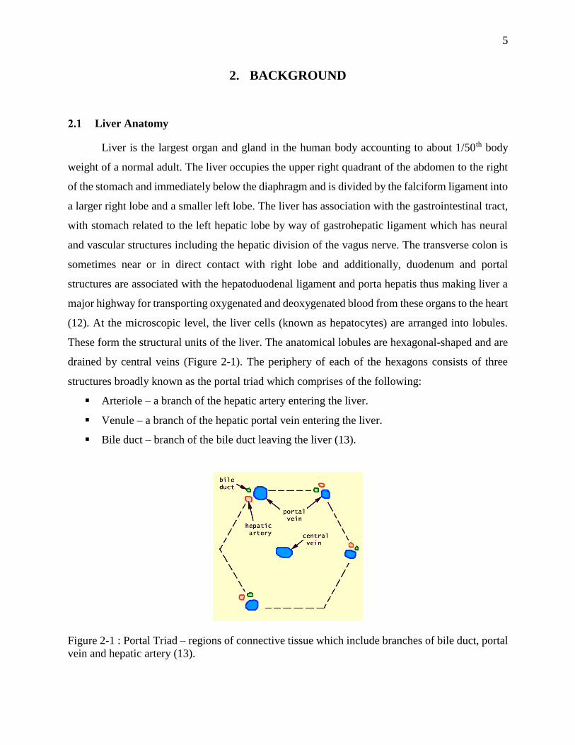
(12). At the microscopic level, the liver cells (known as hepatocytes) are arranged into lobules.

These form the structural units of the liver. The anatomical lobules are hexagonal-shaped and are

drained by central veins (Figure 2-1). The periphery of each of the hexagons consists of three

structures broadly known as the portal triad which comprises of the following:

Arteriole – a branch of the hepatic artery entering the liver.

Venule – a branch of the hepatic portal vein entering the liver.

Bile duct – branch of the bile duct leaving the liver (13).

Figure 2-1 : Portal Triad – regions of connective tissue which include branches of bile duct, portal

vein and hepatic artery (13).

6

The liver aids the digestion of food thereby producing vital nutrients and excretion of waste

material from the body. The liver plays several vital roles such as metabolizing the breakdown

products of digestion and detoxifying substances that are harmful to the body. The liver also

provides essential energy producing substances. The liver controls the production and excretion of

cholesterol and metabolizes alcohol into mild toxin. It also performs many important functions

including storing iron, maintain hormonal balance, producing immune factors, regulating blood

clotting, and producing bile (14).

Liver Biopsy

Liver biopsy is a minimally invasive method of taking a small section of tissue from the

liver and looking under the microscope for signs of damage or disease. It is the gold standard for

diagnosing NASH (non-alcoholic steatohepatitis) and assessing stages of fibrosis patients with

NAFLD (non-alcoholic fatty acid liver disease). NAFLD is a spectrum of diseases varying from

least severe steatosis, to more severe and progressive steatohepatitis to the most severe phenotype

of disease; NASH with advanced fibrosis and cirrhosis. It is mainly caused by deposition of fat in

the liver and it affects individuals with metabolic disorders like obesity, hypertension, diabetes,

hypertriglyceridemia and hyperlipidemia.

Liver biopsy procedure is conducted to determine the cause of abnormal liver function,

swelling or enlargement of the liver and jaundice. These signs and symptoms are due to a variety

of conditions including cirrhosis, hepatitis or cancer (15).

The most commonly used liver biopsy method is percutaneous biopsy where ultrasound

imaging is used to guide a needle into the liver. A numbing medication is injected to the area where

the needle is inserted by making small incision near the bottom of the rib cage on the right side are

done to obtain the liver sample. The tissue sample is fixed in zinc tris at 4°C for 24 hours followed

by chemical processing steps after which the sample is divided into sections of 5 micrometer

thickness for further analysis under a microscope by different staining methods. The current study

used two stains:

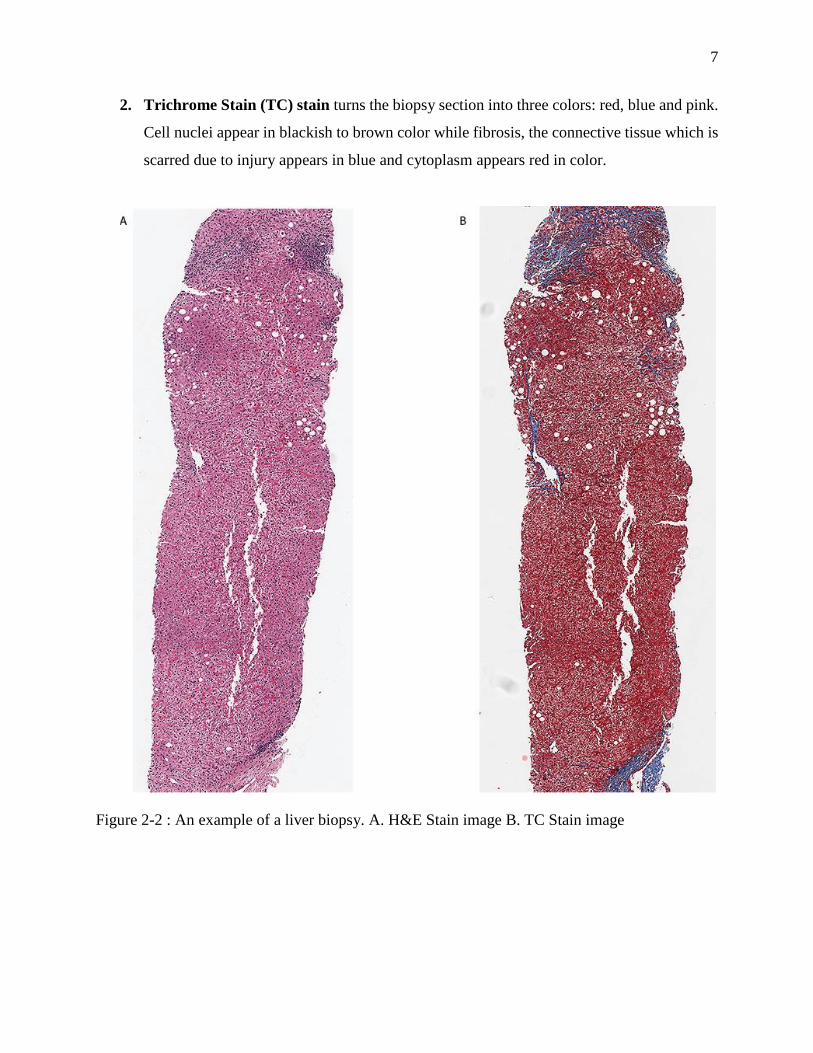
1. Hematoxylin and Eosin Stain (H&E) stain helps in making the biopsy section turn pink

and blue shades which aids in identifying different areas of the cells. Cell nuclei appear in

shade of blue and the cytoplasm in pink.

7

2. Trichrome Stain (TC) stain turns the biopsy section into three colors: red, blue and pink.

Cell nuclei appear in blackish to brown color while fibrosis, the connective tissue which is

scarred due to injury appears in blue and cytoplasm appears red in color.

Figure 2-2 : An example of a liver biopsy. A. H&E Stain image B. TC Stain image

8

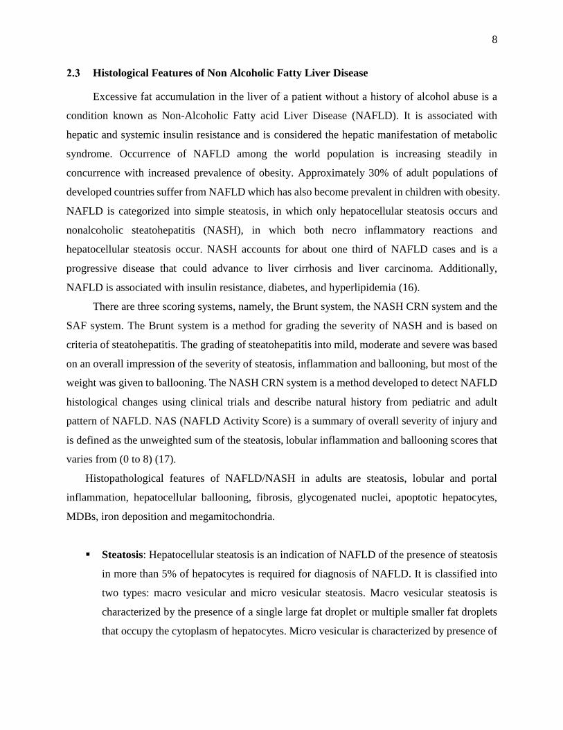
Histological Features of Non Alcoholic Fatty Liver Disease

Excessive fat accumulation in the liver of a patient without a history of alcohol abuse is a

condition known as Non-Alcoholic Fatty acid Liver Disease (NAFLD). It is associated with

hepatic and systemic insulin resistance and is considered the hepatic manifestation of metabolic

syndrome. Occurrence of NAFLD among the world population is increasing steadily in

concurrence with increased prevalence of obesity. Approximately 30% of adult populations of

developed countries suffer from NAFLD which has also become prevalent in children with obesity.

NAFLD is categorized into simple steatosis, in which only hepatocellular steatosis occurs and

nonalcoholic steatohepatitis (NASH), in which both necro inflammatory reactions and

hepatocellular steatosis occur. NASH accounts for about one third of NAFLD cases and is a

progressive disease that could advance to liver cirrhosis and liver carcinoma. Additionally,

NAFLD is associated with insulin resistance, diabetes, and hyperlipidemia (16).

There are three scoring systems, namely, the Brunt system, the NASH CRN system and the

SAF system. The Brunt system is a method for grading the severity of NASH and is based on

criteria of steatohepatitis. The grading of steatohepatitis into mild, moderate and severe was based

on an overall impression of the severity of steatosis, inflammation and ballooning, but most of the

weight was given to ballooning. The NASH CRN system is a method developed to detect NAFLD

histological changes using clinical trials and describe natural history from pediatric and adult

pattern of NAFLD. NAS (NAFLD Activity Score) is a summary of overall severity of injury and

is defined as the unweighted sum of the steatosis, lobular inflammation and ballooning scores that

varies from (0 to 8) (17).

Histopathological features of NAFLD/NASH in adults are steatosis, lobular and portal

inflammation, hepatocellular ballooning, fibrosis, glycogenated nuclei, apoptotic hepatocytes,

MDBs, iron deposition and megamitochondria.

Steatosis: Hepatocellular steatosis is an indication of NAFLD of the presence of steatosis

in more than 5% of hepatocytes is required for diagnosis of NAFLD. It is classified into

two types: macro vesicular and micro vesicular steatosis. Macro vesicular steatosis is

characterized by the presence of a single large fat droplet or multiple smaller fat droplets

that occupy the cytoplasm of hepatocytes. Micro vesicular is characterized by presence of

9

tiny fat droplets with the nuclei centrally located in the cell. Macro vesicular is the most

prevalent form of steatosis with micro vesicular steatosis accounting to approximately

10% of liver biopsies from patients with NAFLD.

Lobular inflammation: Acinar (lobular) inflammation in NAFLD is a mild response from

mixed, acute and chronic inflammatory-cell infiltrate composed of lymphocytes,

monocytes, macrophages and neutrophils with sinusoids and eosinophils occasionally

present. In NASH, the inflammatory cells are usually seen near the site of injured

hepatocytes. Lobular inflammation is evaluated by measuring the number of necro

inflammatory foci per 20x optical field, and by definition, it measures the cluster of

inflammatory nuclei that appear spatially together.

Portal Inflammation: In adult NAFLD, portal inflammation is usually chronic and mild.

When lobular inflammation is disproportionate to portal inflammation, it is an indication

of chronic viral hepatitis C. In a different scenario, suspicion of alcoholic or cholestatic

liver disease is increased when neutrophils infiltrate into the portal and periportal regions.

Also, increased portal inflammation is a marker of advanced disease in untreated NAFLD

patients (18).

Hepatocyte Ballooning: It is characterized by the increase in hepatocyte size of 2 to 3

times its normal healthy size and presence of Mallory’s hyaline in cytoplasm indicating

damaged intermediate filaments within hepatocytes due to disintegration of nuclei in

ballooned cells (16).

Fibrosis: In NASH, perisinusoidal and pericellular fibrosis is a characteristic of fibrosis

which usually begins in zone 3 which is evaluated by reticulin staining. In NAFLD it is

usually observed with an active inflammatory reaction. By general definition, it is the

development of excessive fibrous tissue by the liver when hepatocytes are damaged

eventually leading to cirrhosis.

10

Previous Work

There have been various research studies to detect NAFLD. Some of them use invasive

methods while others use non-invasive techniques. There have been multiple studies to detect

macrosteatosis and fibrosis, some of them even trying to quantify them based on different scoring

patterns. Apart from Vanderbeck et al. (7-9) and Morusu et al.’s (5, 6) continuous study to

automatically analyze macrosteatosis and lobular and portal inflammation, there has been no other

study that has had a big impact. The automatic detection of different types of fibrosis detection

and of microsteatosis is a new contribution of this thesis.

2.4.1 Steatosis

This section gives a brief overview of the literature associated to the detection of steatosis

in liver biopsies. In the previous studies done by Vanderbeck et al. (7-9) and Morusu et al. (5, 6)

detection of macrosteatosis has been done to some extent. In this research, our work optimizes and

improves their approaches in macrosteatosis detection. In addition, it detects microsteatosis.

Steatosis is a common liver disease associated with social and genetic factors which can turn into

cirrhosis. Early detection and quantification is necessary as further delay would evolve it into

cirrhosis.

Ribeiro et al. describes a new non-invasive computer aided diagnosis (CAD) system for

steatosis classification and analysis where Bayes factor, obtained from objective intensity and

textural features extracted from Ultrasound (US) images of liver, is computed on a local and global

basis (19). Each of the US images were stored in the Digital Imaging and Communications in

Medicine (DICOM) format and a region of interest (ROI) of approximately 100 x 100 were

extracted. The main features were extracted using the wavelet transform and autoregressive (AR)

models. A sum of 36 features were extracted from ROI and four types of classifiers (KNN, Bayes

and SVM (polynomial and radial-basis kernel)) were applied to the images. The procedure has

shown an overall accuracy of 93.54% with sensitivity of 95.83% and 85.71% for normal and

steatosis class for 75 patients. Global and local assessment of liver tissue based on the results of

Bayes factor provides useful information to the physicians about the confidence of class. Further

studies are needed to validate the results for more number of patients.

In another research paper, Homeyer et al. describe a new method in identification of fat

droplets in histological images derived from liver biopsy (20). It follows a 2-step process, one that

11

classifies individual pixels as either background or tissue and the second step classifies blobs of

connected background pixels into fat droplets or empty spaces based on their shape. Typically,

background images should be brighter and less saturated than tissue pixels therefore each pixel is

classified by thresholds to their brightness and saturation values. In the second step, the blob

classification step typically is done by performing a connected component labeling operation

which identifies locally connected background pixel as individual blobs followed by a

classification operation that classifies all blobs into fat droplets or empty spaces. Here the classifier

used for the second step is Random Forest Classifier with adjacency statistics, size and eccentricity

being the features. Correlation to pathologist’s scoring was not used to assess accuracy but

repeated random sub-sampling validation of fat droplets was used that showed 90% sensitivity and

specificity.

2.4.2 Inflammation

This section discusses the existing methods for detection of inflammation. In the previous

studies done by Vanderbeck et al. (7-9) and Morusu et al. (5, 6) detection of inflammation has

been done to some extent and this research optimizes and improves their approaches.

In a review paper, Robinson et al. discusses about liver immunology and its role in

inflammation and homeostasis and highlights few key concepts like the myeloid and lymphoid

resident immune cell populations are in large proportions in liver (21). According to this paper,

inflammatory mechanisms are responsible for maintaining local organ and systemic hemostasis in

a healthy liver. But excessive or dysregulated inflammatory activity leads to the pathology

associated with autoimmune and infectious hepatic disease. The hepatic environment is highly

influenced by high fat and carbohydrate diet in the hepatic blood supply. Carbohydrates are usually

stored as glycogen whereas, dietary fat transported from the gut are chylomicrons that are

processed into lipoproteins. The lipoproteins and carbs contain cholesterol, triglycerides and

succinate that trigger inflammatory response by promoting TLR signaling and inflammasome

activation. This metabolic regulation of inflammation is important in non-alcoholic fatty liver

disease. The detection of inflammation is possible by liver biopsy which is a minimally invasive

diagnostic test currently considered to be the “gold standard”.

12

Generally, inflammation is an immediate response to an injury near the site. A lobular

inflammation in NAFLD is a mild response from mixed acute and chronic inflammatory-cell

infiltrate composed of lymphocytes, monocytes, macrophages and neutrophils. A portal

inflammation in NAFLD is a chronic to mild response and it is an accumulation of neutrophils

infiltrate in portal and periportal regions. Previously, the detection of different kinds of

inflammation, which play a role in NAFLD, used semi-quantitative methods that are subjective

and they lacked experienced pathologists to validate (18).

2.4.3 Fibrosis

This section discusses the evolution of methods for evaluating fibrosis. There have been

various studies involving the detection of fibrosis in liver biopsies, however, the studies either lack

the validation from the expert pathologists or do not detect all the different types of fibrosis. Let

us discuss a few of the methods already proposed in the literature.

Masseroli et al. discuss FibroQuant as a robust, reproducible and rapid method for precisely

quantifying the degree of hepatic fibrosis as opposed to semi-quantitative methods (22). These

semi-quantitative methods do not describe the localization and the pattern of hepatic lesions. Their

scoring methodology is inefficient for precise quantifications and is not sufficiently sensitive to

detect small changes in fibrosis. Thus, computerized digital image analysis for precise

quantification of liver fibrosis was proposed which does better than semi-quantitative methods. It

also correlates well with calorimetric method, which quantifies total collagen in a tissue section.

The method enables separate quantification on a single liver histologic image of perisinusoidal,

perivenular, and portal-periportal and septal fibrosis, and portal-periportal and septal morphology.

This automatic segmentation of fibrosis areas produced different intra- and interoperate results,

which is an important step in the prognosis of hepatic diseases. However, the disadvantage of this

method is the lack of an experienced pathologist to validate the results which therefore, undermines

the efficiency and validity of the method.

As semi-quantitative methods proved to be inefficient because evaluation of fibrosis is

subjectively dependent on the visual interpretation by the observer who is not an experienced

pathologist, a recent study by Dahab et al. uses quantification of fibrosis by computer software

using image processing techniques (23). This method answers a few of the pitfalls of semi-

13

quantitative methods by looking at the stained biopsies. The software handles images acquired

from stained connective tissues of liver and converts it into a binary image, applying shading

correction and automatic thresholding, thus extracting the fibrosis area from digitized black and

white image. Further, a polygon around the fibrosis area and lumen areas is drawn manually and

a set of Boolean operations are performed allowing the calculation of the total area of the region

of interest. Such a method results in many errors because processes like thresholding and

converting color images into grayscale discard image information that could be useful in assessing

the contours of the image more accurately. Extracting perisinusoidal or multifocal fibrosis by this

method is impossible adding calculative errors to the method. Finally, considering only sections

of the image would add bias because comparison between tissue patterns must be performed in a

global fashion. This method also lacks an experienced pathologist to validate, and does not address

other regions of fibrosis and does not classify each type of fibrosis.

The next method by Dioguardi et al. claims to be highly objective so far compared to several

qualitative, semi-quantitative and digitized image processing methods by using completely

automated methods (24). The principle of this method is the theory of measurement of all clustered

and non-clustered inflammatory cells. By using specific formulas mentioned in the paper, the

authors offer a geometrically described morphometry of the histological picture for a liver biopsy.

The paper only discusses if the fibrosis is normal or not normal based on calculating different

hematological indices which are either dispersed or clustered but are do not individually classify

each type of fibrosis based on collagen content and several other morphological characteristics

(24).

14

3. METHODOLOGY

This thesis is an extension and improvement of Vanderbeck et al. (7-9) and Morusu et al.’s

study (5, 6) to build models using supervised machine learning techniques for detection of different

histological features which in turn aid in the diagnosis of NAFLD. This study addresses the

identification of various histological features like macrosteatosis and microsteatosis, portal

inflammation and lobular inflammation, and also detecting different types of fibrosis including,

normal fibrosis, pericellular fibrosis, portal fibrosis, periportal fibrosis, bridging fibrosis, and

nodules.

For this study, liver biopsies are taken from human or mice liver, scanned and digitized to

which low-level image processing techniques followed by machine learning techniques are applied.

These liver biopsies are assigned semi-quantitative grades by expert pathologists. The expert

pathologists are provided with a web-based annotation tool, which enables them to annotate

different histological features in a liver biopsy providing class labels which are then used for

building supervised machine learning models. Image processing is performed on the liver biopsy

slide images to extract image features. Firstly, background/foreground extraction is used to

identify the tissue area in the image.

One sub-component of the system is developed to identify and quantify steatosis in the liver

biopsy. Once the tissue area is identified, using different segmentation methods, white regions in

the liver biopsy are detected which are then used for steatosis identification. Based on the

annotations provided by the pathologists, a supervised machine learning model is built by

extracting different types of features like morphological features, texture based features and scale-

space representation features to identify different kind of white regions in the slide. The white

region extraction technique is diagrammatically explained in Figure 3-9. Once the model is built,

unseen samples of liver biopsies are input to the model which then detects and quantifies the

amount of microsteatosis and macrosteatosis. The percentage of steatosis calculated is thus

correlated with the semi-quantitative grades given by the experts.

A second sub-component is developed to detect inflammation in the biopsy images. The first

step in inflammation detection is the detection of the dark regions in an image. This involves

similar methods defined to detect the tissue area and the nuclei in steatosis extraction, and then

extraction of different kinds of features to detect dark regions in the liver biopsy. Once the dark

15

regions in a liver slide are identified, the percentage of lobular and portal inflammation in a tissue

is quantified and is thus correlated with the semi-quantitative grades provided by the expert

pathologists.

Figure 3-1 : The flow diagram presenting the overall approach.

The third sub-component is the detection and classification of various types of fibrosis in the

liver biopsy. The approach to detect different kinds of fibrosis is explained in the Figure 3-14. This

involves the extraction of blue regions in a TC stained liver biopsy using image segmentation

techniques. In order to detect the various types of fibrosis, supervised machine learning models

are built to detect each type separately, involving the extraction of blue regions in an image and

16

performing various feature extraction techniques on the regions annotated by experts, which help

uniquely identify the type of fibrosis content.

Types of Biopsy Data Used

In this study, there are two sources of liver biopsy data used, namely, mice liver and human

liver biopsies. The use of mice liver biopsies can be useful under certain situations and can be

more easily obtained. Moreover, the protein coding regions of mice and human genomes are 85%

identical on an average (some genes are 99% identical, while others are 60% identical) (25).

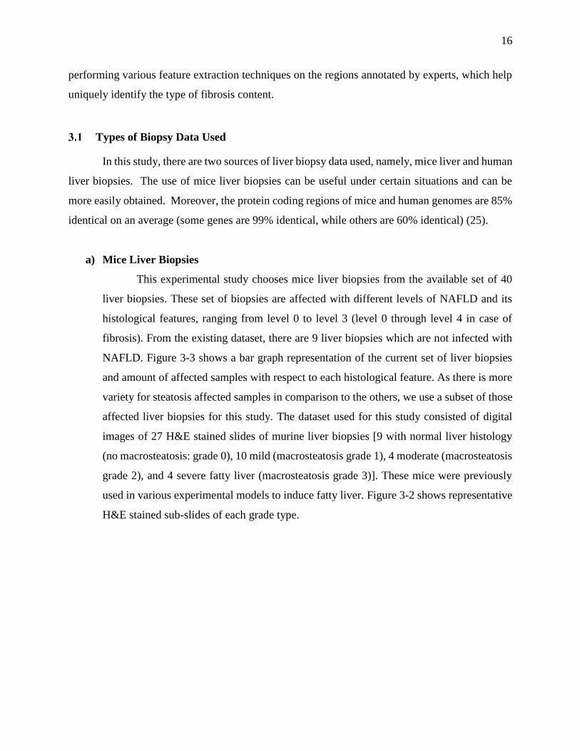
a) Mice Liver Biopsies

This experimental study chooses mice liver biopsies from the available set of 40

liver biopsies. These set of biopsies are affected with different levels of NAFLD and its

histological features, ranging from level 0 to level 3 (level 0 through level 4 in case of

fibrosis). From the existing dataset, there are 9 liver biopsies which are not infected with

NAFLD. Figure 3-3 shows a bar graph representation of the current set of liver biopsies

and amount of affected samples with respect to each histological feature. As there is more

variety for steatosis affected samples in comparison to the others, we use a subset of those

affected liver biopsies for this study. The dataset used for this study consisted of digital

images of 27 H&E stained slides of murine liver biopsies [9 with normal liver histology

(no macrosteatosis: grade 0), 10 mild (macrosteatosis grade 1), 4 moderate (macrosteatosis

grade 2), and 4 severe fatty liver (macrosteatosis grade 3)]. These mice were previously

used in various experimental models to induce fatty liver. Figure 3-2 shows representative

H&E stained sub-slides of each grade type.

17

Figure 3-2 : Representative Hematoxylin and Eosin images of different models used to induce fatty

liver. A. Normal liver in wild type mouse fed chow diet. B. Mild fatty liver in wild type mouse fed

high fat diet. C. Moderate fatty liver in GFP-LC3 mouse fed alcohol. D. Severe fatty liver in GFP-

LC3 mouse fed high-fat high-carbohydrate diet.

All animal experimental protocols were approved by the Institutional Animal Care

and Use Committee of Indiana University (IACUC). Animals were housed under approved

conditions with 12 hour light dark cycle. C57BL/6 wild type and GFP-LC3(26) were bred

in house. At 10 weeks of age, mice were placed on normal chow diet to produce normal

liver, high fat diet (diet D12492, Research diets) to produce mild fatty liver or high-fat

high-carbohydrate (HFHCD) diet, or chronic alcohol (29-36%) to produce moderate to

severe fatty liver. For HFHCD diet, mice were given high fat diet along with the drinking

water enriched with high-fructose corn syrup equivalent to a total of 42 g/L of

carbohydrates. Drinking solution was made by mixing in drinking water at a ratio of 55%

fructose (Acros Organics, Morris Plains, NJ) and 45% sucrose (Sigma- Aldrich, St. Louis,

MO) by weight. Animals were provided ad libitum access to these diets for 10-24 weeks.

Only liver biopsy slides from prior concluded studies were utilized for this study. Mice

were first given Avertin (250 mg/kg, i.p.) for anesthesia, followed by cervical dislocation

for euthanization. This procedure minimizes any suffering. All procedures are approved by

the IACUC of Indiana University.

18

Liver biopsy H&E stained slides were studied and scored by the pathologist Dr. C

according to NASH Clinical Research Network scoring system where steatosis grade range

between 0-3 ( 0 < 5% steatosis , 1 = 5% - 33%, 2 = 33% - 66%, and 3 > 66% ) (27).

Figure 3-3 : Pictorial representation of number of mice liver biopsies graded by Dr. C.

b) Human Liver Biopsies

This experimental study chooses from 66 human liver biopsies. Both the

pathologists mentioned below in Section 3.3, namely Dr. K and Dr. C, provided semi-

quantitative grades for the human liver biopsies. Dr. K graded 64 of the available 66 liver

biopsies, however, Dr. C graded all the present human liver biopsies. Figure 3-5 and Figure

3-6 show the bar graph representation of different patients affected with each histological

feature of NAFLD based on the both the experts’ semi-quantitative grades. For this study,

the H&E stained liver biopsies are used for detection of lobular and portal inflammation

and correlated with the pathologist grades, and the TC stained liver biopsies are used for

the detection of different types of fibrosis. There are 11 slides which are not affected by

NAFLD. These human liver slides were previously used for experimental study as well.

0

10

20

30

40

Steatosis PortalInflammation

LobularInflammation

HepatocyteBallooning

Fibrosis

Nu

mb

er o

f Sa

mp

les

Type of NAFLD Lesion

Grade 0 Grade 1 Grade 2 Grade 3

19

Figure 3-4 : Pictorial representation of number of human liver biopsies graded by Dr. K.

Figure 3-5 : Pictorial representation of number of human liver biopsies graded by Dr. C.

Image Data

To obtain the digitized images, the biopsy slides are scanned at 20X using Aperio Scan

Scope CS system. The scanned images are stored in SVS file format. These are based on the TIFF

format of images at multiple resolutions and utilizes the tile image capabilities. They use

compression type 33005 (which is a specific kind of JPEG 2000 compression for RGB format).

Each SVS file received contains different types of images. The first one is termed as the

“baseline version of the image” i.e. contains the full resolution version of the image. The second

image is generally a thumbnail version, typically having dimensions of about 1024 × 768 pixels

05

10152025303540


LobularInflammation


FibrosisN

Um

ber

of

Sam

ple

s


Grade 0 Grade 1 Grade 2 Grade 3 Grade 4

0

5

10

15

20

25

30

35


LobularInflammation


Fibrosis

Nu

mb

er o

f Sa

mp

les


Grade 0 Grade 1 Grade 2 Grade 3 Grade 4

20

which is always stripped. All the remaining versions of the image are pyramid images (each having

lower resolution than the previous by a factor of 2 in each dimension), which are compressed with

the same type of compression as that of the baseline image, organized as tiles with same tile size.

The last two version of the image however, is a slide label image which contains lower resolution

of either the slide label or the slide itself. Our research involves extraction of the highest resolution

image (in JPEG format) and using a 50% reduced version of it, which enables us to speed up our

image processing activities.

Pathologist Grades and Annotations

This study involves getting expert pathologists to grade the biopsy slide based on the

NASH scoring system and also annotate different histological features in liver biopsy images. In

this study, two pathologists provided the annotations and semi-quantitative grades for the liver

biopsy slides. The different biopsy images include both a TC Stained and H&E Stained variants,

such that the former is used for labeling and grading fibrosis content while the latter is used for

labeling and grading steatosis, inflammation and ballooning content. The pathologists are Dr

David E. Kleiner and Dr Oscar W. Cummings. Dr. David E. Kleiner, M.D., Ph.D. currently heads

the Histopathology and Autopsy Pathology department at the Center of Cancer Research at

National Cancer Institute in National Institute of Health (NIH) located at Bethesda, Maryland,

United States (referred as Dr. K in this study). Dr. Oscar W. Cummings, M.D. is a Professor of

Pathology and Laboratory Medicine and the Director of Surgical Pathology at Indiana University

School of Medicine located at Indianapolis, Indiana, United States (referred as Dr. C in this study).

All experiments conducted in this study to build different decision support systems to detect

various histological features in a liver biopsy use both the above mentioned pathologists’

annotations for building machine learning models and their semi-quantitative grades for

correlation.

3.3.1 Annotation Tool

One of the most important steps in this research involves gathering data from the expert

pathologists. A web annotation tool had been built to annotate slide images and store the

annotations (11). This tool is built using HTML5 and javascript open source technologies like

Open Layers (currently under BSD License), which provides application programming interfaces

21

(APIs) to build rich web-based applications and Bootstrap (v3) which enhances the look and feel

of the tool by providing responsive HTML and CSS enhancements.

Vanderbeck et al in his study (7-9) had developed a web application for getting annotations

from the experts. However, only small scaled images could be used to accomplish the same.

Because of the size of our high resolution liver biopsy slides, that application could not be used.

The markers associated with the tool were not user friendly and very large images take a lot of

time to load. Later, Morusu et al. in her study (5, 6) developed a web application tool which

addresses some of the above mentioned issues. In her study, she used the Open Layers API to load

very large images at a quicker pace, such that images are divided into different set of tiles, and

only the required set of tiles were loaded during annotation. However, the tool lacked some

functionality in the labeling of TC Stained samples with different levels of fibrosis and the usability

of the tool was not possible in different resolution monitors and browsers. Apart from this, the

above mentioned tool had different setups for mice liver biopsies and human liver biopsies. To

overcome all the above mentioned challenges, a responsive user interface (using Bootstrap library)

has been added so that different type of screen resolutions do not hinder the usage of the tool.

Along with the list of annotation labels mentioned by Morusu et al., new labels have been added

for TC stained images to identify many more histological features which help uniquely identify

the respective types. Figure 3-6 and Figure 3-7 give an overview of the newly built annotation tool.

In adherence to Morusu et al.’s idea (5, 6) of annotating slides two ways, the newly built

annotation tool thus provides, point annotations as well as polygon annotations. Additionally, there

is a newly added subset of polygon annotations, termed as square annotations which are used to

identify the different types of fibrosis. This eases the work for the pathologist to draw a regular

polygon, instead provides with an in-built square with a feature to expand the same. Flat files

(unique by the combination of the image name and pathologist username), are used to save the

annotations at the back end.

There are point annotations which are used to annotate relatively distinct areas of the image

i.e. regions which have a specific shape, and structure. Therefore, the coordinates of the point are

stored along with the anatomical/histological structure it defines is written in a file at the back end.

There are polygon annotations which are also known as boundary annotations, that enable

the pathologist to annotate structures which have irregular shapes, but are convex in nature. Each

click creates an edge in the polygon as we go along annotating it, a double click indicates that the

22

region is identified. Hence, the coordinates along each edge are recorded apart from the number

of edges and the anatomical/histological structure it defines in a file at the back (server) end.

There are special type of polygon annotations introduced termed as square annotations,

which allows the user to annotate areas in an expandable square format. This type of annotation

has been introduced to ease the adding of an annotation. Thus, the coordinates along each edge are

recorded with a fixed number of edges (=4) and the anatomical/histological structure it defines at

the back end.

Annotation

Name

Annotation

Type Description

Annotation

Color

Macro Fat Point Distinct globular white regions,

generally in circular structure. Magenta

Micro Fat Polygon Soapy textured white regions,

spread across the biopsy area. Dark Blue

Normal

Fibrosis

Square

Polygon

Blue regions around the

inflammation area.

Yellow

(Fill)

Pericellular

Fibrosis

Square

Polygon

Coarse chicken wired blue region

structures around the cell areas. Red (Fill)

Portal

Fibrosis

Square

Polygon

Blue regions around the portal vein

areas. Aqua (Fill)

Periportal

Fibrosis

Square

Polygon

Extension of blue regions around

portal fibrosis. Purple (Fill)

Bridging

Fibrosis

Square

Polygon

Continuous flow of blue regions

spread across bile duct and any vein. Lime (Fill)

Nodules Square

Polygon

Elliptical structures of comprising

of blue region borders. Teal (Fill)

Hepatocyte

Ballooning Polygon

Dark region areas across which

appears with wispy cytoplasm. Magenta

Lobular

Inflammation Polygon

Dark region areas which show

inflammatory nuclei. Teal

Portal

Inflammation Polygon

Dark region areas showing

inflammatory nuclei in portal

regions.

Lime

As discussed by Morusu et al.(5, 6) in her study, the Table 3-1 presents a list of the current

supported histological/anatomical structures in a liver biopsy. Each of the structures have a type

of color associated with them in the annotation tool in order to differentiate them from one another.

Table 3-1 : The different types of annotations present in the web annotation tool.

23

There are two figures – Figure 3-6 and Figure 3-7 that demonstrate point and boundary annotation

examples in a mice liver biopsy and some square annotations in a human liver biopsy, respectively.

Figure 3-6 : A Preview of the mice liver labeling tool with point and boundary annotations labeled

at 6x magnification.

Figure 3-7 : A Preview of the human liver labeling tool with square annotations (fibrosis

annotations) labeled at 6x magnification.

a. NAFLD Lesions: The set of annotations in Tables 3-2 and 3-3 constitute the histological

features in the liver biopsy which are essential to determine if a person is affected with

NAFLD. Fibrosis and its types are present only in TC stained liver biopsies.

24

Tables 3-2 and 3-3 show the number of annotations provided by the expert pathologist(s)

(Dr. C) in mice liver and (Dr. C and Dr. K) in human liver biopsies.

Table 3-2 : The number of NAFLD lesion annotations present for mice liver biopsies.

Annotation

Name

Annotations – Dr. C

Macro Fat 22696

Micro Fat 568

Hepatocyte

Ballooning

0

Lobular

Inflammation

40

Portal

Inflammation

28

Table 3-3 : The number of lesion annotations present for human liver biopsies.

Annotation

Name Annotations – Dr. C Annotations – Dr. K

Total

Annotations

Macro Fat 952 359 1311

Micro Fat 0 12 12

Normal

Fibrosis 0 186 186

Pericellular

Fibrosis 126 128 254

Portal

Fibrosis 2 118 120

Periportal

Fibrosis 46 127 173

Bridging

Fibrosis 41 98 139

Nodules 54 61 115

Hepatocyte

Ballooning 11 92 103

Lobular

Inflammation 260 347 607

Portal

Inflammation 163 340 503

b. Anatomical Structures in liver biopsy: The set of annotations in Table 3-4 constitute the

different anatomical structures present in a liver biopsy.

25

Annotation

Name

Annotation

Type Description

Annotation

Color

Bile Duct Polygon Ring - like white region structures,

generally with nuclei. Orange

Central Vein Polygon White region structure around the

center of a lobular area. Green

Portal Artery Polygon White regions showcasing a thick

arterial wall. Aqua

Portal Vein Polygon

White regions in general. A blood

vessel which carries blood from

different areas around to the liver.

Blue ring

(with red

fill)

Sinusoid Point

White region generally, blood vessel

between hepatic artery and portal

vein

Yellow

Table 3-5 shows the number of annotations provided by the expert pathologist (Dr. C) in

mice liver. Table 3-6 shows the number of annotations provided by both pathologists (Dr.

C and Dr. K) in human liver biopsies.

Table 3-5 : The number of annotations present for mice liver biopsies.

Annotation

Name Annotations – Dr. C

Bile Duct 121

Central Vein 117

Portal Artery 22

Portal Vein 75

Sinusoid 39

Table 3-4 : The different anatomical structures present in a liver biopsy.

26

Table 3-6 : The number of annotations present for human liver biopsies.

Annotation

Name

Annotations – Dr.

C

Annotations – Dr. K Total Annotations

Bile Duct 43 115 158

Central Vein 13 50 63

Portal Artery 32 72 104

Portal Vein 37 80 117

Sinusoid 314 173 487

c. Control Tissues: The tissue areas which serve as normal regions or areas where the disease

is not present (Table 3-7).

Annotation

Name

Annotation

Type Description

Annotation

Color

Normal

Hepatocyte Polygon

Liver cells – occupy 80% of the

liver in general. Red

Normal

Parenchyma Polygon

Group of liver cells which perform

a particular activity.

Aqua ring

(with orange

fill)

Tables 3-8 and 3-9 show the number of annotations provided by the expert pathologist(s)

(Dr. C) in mice liver and (Dr. C and Dr. K) in human liver biopsies.


Annotation

Name


Normal

Hepatocyte

10

Normal

Parenchyma

6

Table 3-7 : The different types of control tissues.

27


Annotation

Name

Annotations – Dr. C Annotations – Dr. K Total

Annotations

Normal

Hepatocyte

1 52 53

Normal

Parenchyma

0 11 11

d. Others: These are the areas which are incorporated due to the process involving in taking

a liver biopsy and preparing the slides (Table 3-10). These account for negative classes in

our study.

Annotation

Name

Annotation

Type Description

Annotation

Color

Tissue

Preparation

Tear

Point Tissue tear during tissue

preparation. Generally white region. Orange

Tissue

Preparation

Stretch

Point Tissue stretch during tissue

preparation. Generally white region. Dark Blue

Slide

Background Point The non-tissue area in the slide. Lime

Tissue Fold Point Tissue fold during tissue

preparation. Green

Squame Point Structure damage in tissue. Aqua

Other Point Any other structure apart from the

above mentioned ones. Red

Tables 3-11, 3-12, and 3-13 show the number of annotations provided by the expert

pathologist(s) (Dr. C) in mice liver and (Dr. C and Dr. K) in human liver biopsies.

Table 3-10 : A few histological areas incorporated while taking a liver biopsy.

28


Annotation

Name


Tissue

Preparation

Tear

22

Tissue

Preparation

Stretch

11

Slide

Background

0

Tissue Fold 47

Squame 39

Other 5


Annotation

Name

Annotations – Dr. C Annotations – Dr. K Total

Annotations

Tissue

Preparation

Tear

49 102 151

Tissue

Preparation

Stretch

0 0 0

Slide

Background

0 59 59

Tissue Fold 12 25 37

Squame 0 1 1

Other 6 15 21

29

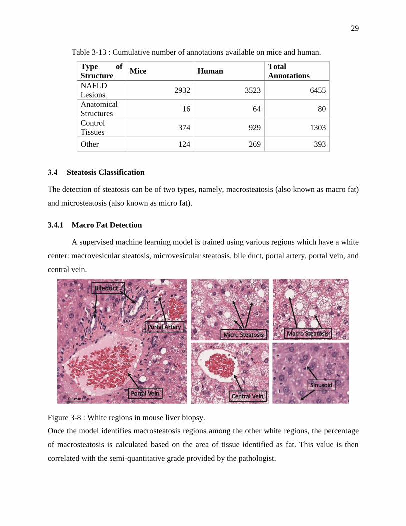
Table 3-13 : Cumulative number of annotations available on mice and human.

Type of

Structure Mice Human

Total

Annotations

NAFLD

Lesions 2932 3523 6455

Anatomical

Structures 16 64 80

Control

Tissues 374 929 1303

Other 124 269 393

Steatosis Classification

The detection of steatosis can be of two types, namely, macrosteatosis (also known as macro fat)

and microsteatosis (also known as micro fat).

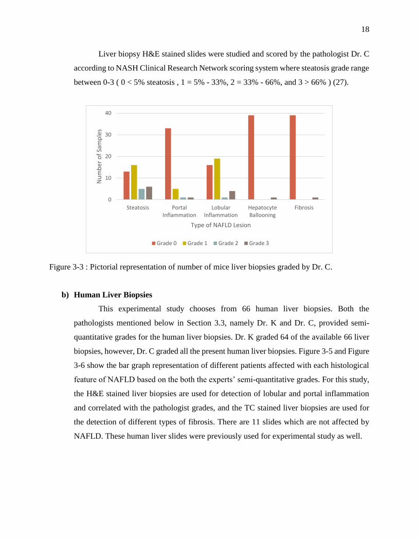
3.4.1 Macro Fat Detection

A supervised machine learning model is trained using various regions which have a white

center: macrovesicular steatosis, microvesicular steatosis, bile duct, portal artery, portal vein, and

central vein.

Figure 3-8 : White regions in mouse liver biopsy.

Once the model identifies macrosteatosis regions among the other white regions, the percentage

of macrosteatosis is calculated based on the area of tissue identified as fat. This value is then

correlated with the semi-quantitative grade provided by the pathologist.

30

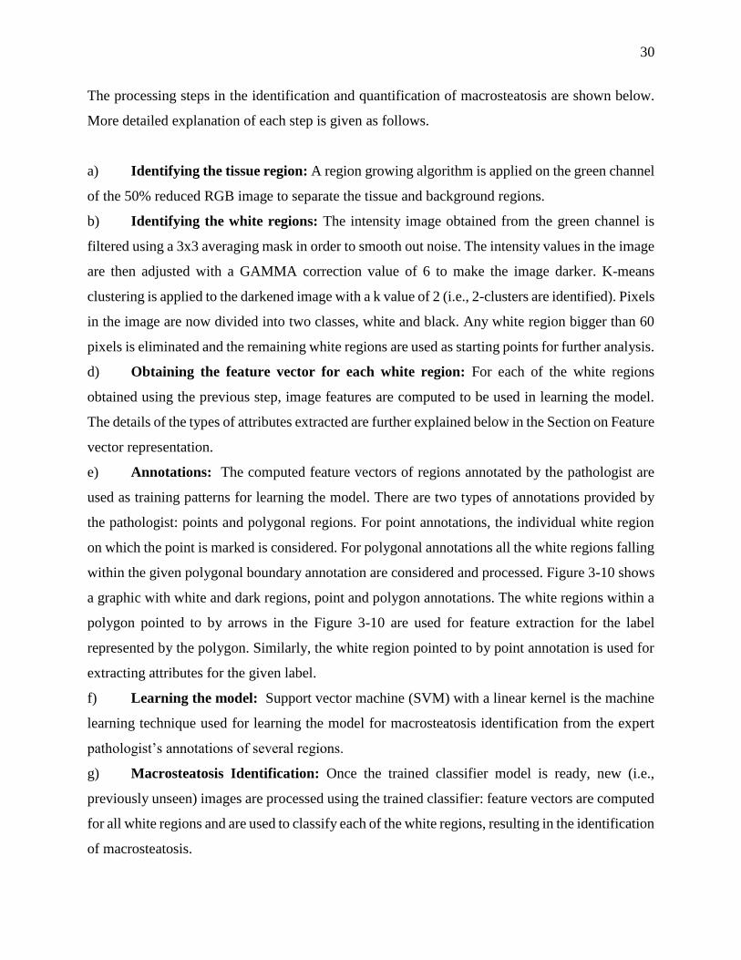
The processing steps in the identification and quantification of macrosteatosis are shown below.

More detailed explanation of each step is given as follows.

a) Identifying the tissue region: A region growing algorithm is applied on the green channel

of the 50% reduced RGB image to separate the tissue and background regions.

b) Identifying the white regions: The intensity image obtained from the green channel is

filtered using a 3x3 averaging mask in order to smooth out noise. The intensity values in the image

are then adjusted with a GAMMA correction value of 6 to make the image darker. K-means

clustering is applied to the darkened image with a k value of 2 (i.e., 2-clusters are identified). Pixels

in the image are now divided into two classes, white and black. Any white region bigger than 60

pixels is eliminated and the remaining white regions are used as starting points for further analysis.

d) Obtaining the feature vector for each white region: For each of the white regions

obtained using the previous step, image features are computed to be used in learning the model.

The details of the types of attributes extracted are further explained below in the Section on Feature

vector representation.

e) Annotations: The computed feature vectors of regions annotated by the pathologist are

used as training patterns for learning the model. There are two types of annotations provided by

the pathologist: points and polygonal regions. For point annotations, the individual white region

on which the point is marked is considered. For polygonal annotations all the white regions falling

within the given polygonal boundary annotation are considered and processed. Figure 3-10 shows

a graphic with white and dark regions, point and polygon annotations. The white regions within a

polygon pointed to by arrows in the Figure 3-10 are used for feature extraction for the label

represented by the polygon. Similarly, the white region pointed to by point annotation is used for

extracting attributes for the given label.

f) Learning the model: Support vector machine (SVM) with a linear kernel is the machine

learning technique used for learning the model for macrosteatosis identification from the expert

pathologist’s annotations of several regions.

g) Macrosteatosis Identification: Once the trained classifier model is ready, new (i.e.,

previously unseen) images are processed using the trained classifier: feature vectors are computed

for all white regions and are used to classify each of the white regions, resulting in the identification

of macrosteatosis.

31

Figure 3-9 : Overall flow diagram of the approach to automated macrosteatosis identification and

quantification.

Figure 3-10 : Graphic showing dark and white regions with point and polygon annotations. The

white region labeled using point annotation (represented using 'X') is used for extracting attributes.

A polygon annotation is shown using black polygon. The white regions falling within the polygon

are indicated by arrows and these are the regions used for attribute extraction for the given label.

3.4.2 Micro Fat Detection

As shown in Figure 3-8, microsteatosis could display different histological appearances on

H&E stained liver biopsies, from very tiny cytoplasmic vesicles, to small cytoplasmic vesicles that

do not displace the hepatocyte nucleus, to a foamy appearance of the cytoplasm. A supervised

machine learning model is trained using various regions: microvesicular fat, macrovesicular fat,

32

bile duct, portal artery, portal vein, central vein and sinusoid. This trained model is then used to

identify the microsteatosis regions in the image among the other identified regions.

The processing steps in the identification of microsteatosis are shown in Fig 3-11. More

detailed explanation of each step is given below.

a) Obtaining the image: The digital image from the Aperio Scan Scope CS system is stored

in Aperio svs format. The resolution picked from svs format file is the 50% reduced one.

b) Identifying the tissue region: A region growing algorithm is applied on the green channel

of the 50% reduced RGB image to separate the tissue and background regions.

c) Obtaining feature vector for region (pixel wise): For each of the images generated after

isolating the tissue area as described in step (b), Gabor filter based texture features are computed.

The details of the feature extraction are further explained below in Section 3.4.3 on Feature vector

representation.

d) Annotations: The computed feature vectors of regions annotated by the pathologist are

used as training patterns for learning the model. In the web-based annotation tool, the

microsteatosis regions are denoted by the pathologist by drawing a polygon around the regions.

The pixels falling within these annotated polygons are labeled as microsteatosis and the computed

features for these pixels are used for training the model. Because the number of such pixels is too

large, in order to reduce the computation time for the training phase, we randomly subsampled

0.02% of the pixels annotated as microsteatosis and 0.001% of the pixels annotated as any other

histological feature.

e) Learning the model: SVM with a linear kernel is the machine learning technique used

for learning the model for microsteatosis identification from the expert pathologist’s annotations

of several regions.

f) Microsteatosis identification: Once the trained classifier model is ready, new (i.e.,

previously unseen) images are processed using the trained classifier: feature vectors based on

Gabor texture features are computed for all regions which are then used to classify them as

microsteatosis or non-microsteatosis regions.

33

Figure 3-11 : Overall flow diagram of the approach to automated microsteatosis identification.

3.4.3 Feature Vector representation

In prior studies presented by Vanderbeck et al. (7-9) and Morusu et al. (5, 6, 11), we used

image texture statistics at various scales (σ = 0,1,2,4,8) as feature vectors to be used as input to the

classifier. In this study, we have extended this feature set to improve the accuracy of identification.

“We added a new set of textural features using Gabor filters (28, 29) in detected white regions or

in annotated macrosteatosis regions. For each of the white regions, the surrounding area of 20

pixels in all directions is considered for extracting these attributes. Also, a rectangular region of

25 pixels around the white region is considered for feature extraction.

Gabor filters, which are band pass filters at various frequencies and orientations, are used

in this study for texture analysis. The impulse response of a Gabor filter is the product of a

sinusoidal plane wave at a given frequency (𝑓 = 1𝜆⁄ ) and orientation (𝜃) with a Gaussian function

at a given scale (𝜎).

The equation of Gabor function in spatial domain is given below (30-33):

𝑔(𝑥, 𝑦; 𝜆, 𝜃, 𝜓, 𝜎) = exp (−𝑥′2 + 𝑦′2

2𝜎2) exp (𝑖 (2𝜋

𝑥′

𝜆+ 𝜓))

where 𝑥′ = 𝑥 cos 𝜃 + 𝑦 sin 𝜃 and 𝑦′ = −𝑥 sin 𝜃 + 𝑦 cos 𝜃, are the rotated coordinates to account

for the filter orientation, 𝜆 = 1 𝑓⁄ is the period of the sine wave, 𝜃 is the orientation of the Gabor

34

filter, 𝜎 is the width of the Gaussian envelope, 𝜓 is the phase offset of the sine wave, and 𝑖 =

√−1. Thus, the function 𝑔(𝑥, 𝑦; 𝜆, 𝜃, 𝜓, 𝜎) defines the convolution kernel. Filtering is performed

in the frequency domain using fast Fourier transforms as it is computationally faster.

In the macrosteatosis identification, we have used four orientations ( 𝜃 =

0°, 45°, 90°, and 135°) for the Gabor filters and for each orientation five radial frequencies which

are one octave apart, for a total of 20 Gabor filters (4 orientations × 5 frequencies) (34). These

filters are applied to 7 images (3 for RGB channels separately, 3 for HSV channels separately and

one for the gray level image) resulting in a total of 140 Gabor filter features.” (5, 6)

These, combined with the features from our prior study (35), results in a total of 554

features which have been used in training the classifier.

In the microsteatosis identification, we have used four orientations ( 𝜃 =

0°, 45°, 90°, and 135°) for the Gabor Filters and for each orientation ten radial frequencies which

are one octave apart, for a total of 40 Gabor filters (4 orientation × 10 frequencies) (34). These

filters are applied to a single image (gray scale), resulting in 40 Gabor filter features for each pixel.

3.4.4 External Validation of Classifier’s Accuracy

To verify the accuracy of the classifiers identifications of lesions as macro- or

microsteatosis, liver biopsy images previously unseen by the classifiers that have not been used in

the training of the classifier were used in this step.

For macrosteatosis validation, fifty randomly identified macrosteatosis lesions were

selected and classified using the automated algorithm. These classification results were examined

by the study pathologist to determine the validity of the identification.

For microsteatosis validation, one hundred and ten random sub slides from a pool of

eleven previously unseen slides were examined by the study pathologist to determine the validity

of the identification. We used a larger number of microsteatosis identified lesions for validation in

order to properly represent the slides based on the significantly smaller size of these lesions

compared to macrosteatosis lesions. The study pathologist assessed each identified (microsteatosis

or not microsteatosis) lesion by the classifier as correct or incorrect. Accuracy was calculated as

percent correctly identified with macro- or microsteatosis by the classifier as determined by the

gold standard, the study expert pathologist.

35

3.4.5 Quantification of Macro Fat

After macrosteatosis regions are identified by the trained classifier, the percent area of

macrosteatosis in a biopsy image was quantified. Pathologists provide semi-quantitative

macrosteatosis grade based on their perception of percentage macrosteatosis area. And hence, in

this study, the ratio of measured macrosteatosis area to the total tissue area is calculated as a

continuous measure of macrosteatosis quantification so that it can be compared with pathologist’s

semi-quantitative grades. For each of the white regions, the area is already calculated as part of

computing the morphological features. The sum of areas of all white regions identified by the

classifier is the macrosteatosis area. The tissue area is computed by using the background mask

extracted in the white region identification process. The image area in the regions where mask is

not present is considered as tissue and the space occupied by this region in pixels is the tissue area.

Inflammation Classification

The identification of inflammation areas include the detection and quantification of each of

the lobular and portal inflammation. This section describes the process of doing the same.

3.5.1 Lobular and Portal Inflammation Detection

This research is an extension of the study done by Morusu et al. to detect inflammation in

human liver biopsies (5, 6). As addressed in the above study, this involves detection of the different

dark regions associated to a liver biopsy sample. The various histological features that are

generally referred to as dark regions include, lobular inflammation, portal inflammation, normal

hepatocyte and bile duct.

36

Figure 3-12 : The different dark regions present in a liver biopsy slide.

The Figure 3-12 shows the each of the different dark regions taken for this study. Here, we

try to improve the existing models built for lobular and portal inflammation detection by reducing

the classes that are not affected much, such as micro fat, tissue folds, normal parenchyma and

hepatocyte ballooning. The same processing techniques (explained by Morusu et al. (5, 6)) are

applied and a supervised machine learning model is created with the above four mentioned

features.

37

3.5.2 External Validation of Classifier’s accuracy

In order to verify the accuracy of detection of the built machine learning classifier for both

lobular and portal inflammation, unseen liver biopsy samples which have not been used as part of

the training set to build the classifier have been used.

To detect the lobular inflammation, there are 113 sub slides selected in random from a set

of 16 liver biopsy slides which are processed and evaluated by the classifier to detect the presence

of lobular inflammation. The results from the classifier are then examined by the expert

pathologists to determine the correctness of the classifier built.

For the portal inflammation detection, there are 110 sub slides selected in random from a

set of 16 liver biopsy slides which are then processed by the built classifier to detect the portal

inflammation areas. These areas are then evaluated by the expert pathologists to determine the

accuracy of the classifier. The accuracy of the classifier is computed based on the ratio of number

of correctly classified instances by the total number of instances processed by the classifier as

determined to the pathologists’ “gold standard”.

3.5.3 Quantification of Inflammation

Once the inflammation regions are identified by the classifier built, the percentages of both

lobular and portal inflammation areas in a biopsy image are quantified. The expert pathologists

provide semi-quantitative grades based on their perception of the infected portal and lobular

inflammation areas. Therefore, in this research, the ratio of measured portal and lobular

inflammation area to that of the tissue is computed and thereby compared to the expert

pathologists’ grades. For each of the dark region computed, the area is computed based on the

morphological features calculated. The tissue mask area is the actual area in the slide with the

tissue present (computed in the step 2 of the process).

Fibrosis Classification

In our study, we look to build a new classifier which detects if fibrosis is present in a liver

biopsy. Apart from this, we also build different classifiers to identify the various types of fibrosis

which include, normal fibrosis, pericellular fibrosis, portal fibrosis, periportal fibrosis, bridging

fibrosis and cirrhosis by analyzing the various blue regions in the image, also known as collagen.

38

Fibrosis is the blue region area present in a TC Stained liver biopsy. Based on their

morphological structures, textural properties and their surrounding neighborhood, they are

identified as different types of fibrosis. While building the model, all labels which have blue

regions associated with the annotated slide are fed to the classifier. During the model’s training

phase, the annotated area’s neighborhood is also analyzed, apart from present annotated region.

As the classifier gets built, unseen samples are passed to the model which in-turn detect the kind

of fibrosis present. The amount of blue region (collagen) is correlated with the pathologist grades

as well. The severity of fibrosis is detected based on the following table. Based on the number of

nodule regions and the bridging regions, followed by the percentage(s) of other types of fibrosis

like, portal fibrosis, periportal fibrosis, pericellular fibrosis and normal fibrosis, we correlate them

with the semi-quantitative grade provided by the pathologists.

Different types of fibrosis classes are listed below along with their diagrammatic

representation.

1. Normal Fibrosis: The blue regions around the inflammatory nuclei (dark regions which

are diffusely scattered). Figure 3-13A shows an example of Normal Fibrosis.

2. Pericellular Fibrosis: The chicken wire shaped blue regions which are very thin around

the cell. These extend along sinusoids to surround one or a group of hepatocytes. Figure 3-

13B shows an example of Pericellular Fibrosis.

3. Portal Fibrosis: The blue regions present around the portal triad region are termed Portal

Fibrosis, which consequently become densely stained and expanded around those regions,

however, there is no extensions to its adjacent parenchyma. Figure 3-13C shows an

example of Portal Fibrosis.

4. Periportal Fibrosis: The blue regions present around the periportal triad region are termed

as Periportal Fibrosis, there can be extensions to its neighboring parenchyma. Figure 3-

13D shows an example of Periportal Fibrosis.

5. Bridging Fibrosis: The connective blue strands present across the tissue connecting

various portal tracts and central veins. They are continuous in nature. Figure 3-13E shows

an example of Bridging Fibrosis.

6. Cirrhosis (Nodule): The blue region strands which when connected, form a regular

elliptical structure is termed as Nodule or Cirrhosis. This type of fibrosis is widely

39

distributed therefore, the resultant morphological structure appearance encompass a wide

spectrum. Figure 3-13F shows an example of Nodule.

Figure 3-13 : Different types of fibrosis annotated. A. Normal Fibrosis B. Pericellular Fibrosis C.

Portal Fibrosis D. Periportal Fibrosis E. Bridging Fibrosis F. Nodule.

There are a number of classifiers built during this process. Firstly, there is one classifier

we build with two classes namely, Normal Fibrosis (represented in Figure 3-14A) and abnormal

fibrosis. The abnormal fibrosis classes consists of all the remaining types of fibrosis ranging from

pericellular fibrosis, portal fibrosis, periportal fibrosis, bridging fibrosis, cirrhosis. Apart from this

classifier, there is another one which contains pericellular fibrosis, portal fibrosis, periportal

fibrosis and bridging fibrosis. The third classifier built has two classes namely, nodules and others

where others constitute pericellular fibrosis, portal fibrosis, periportal fibrosis and bridging fibrosis.

40

3.6.1 Blue region Extraction

The first step involved in identification of different types of fibrosis involves blue region

extraction from a TC Stained image. The following are the steps involved in extracting the collagen

in a liver biopsy. Figure 3-14 gives a pictorial representation of the same.

a. Image Retrieval: The TC Stained image is obtained in Aperio svs format. The image is

then processed in the 50% scaled version of it.

b. Identification of Tissue: In order to identify the tissue area, an 8-bit gray scale image is

created. This distinguishes the tissue area sample from the image background and this is

done by forming a weighted sum of the R, G and B components using the following

formula: 𝑔𝑟𝑎𝑦 = 0.2989 𝑅 + 0.5870 𝐺 + 0.1140 𝐵 (36) The gray image is then

subjected to global thresholding using Otsu’s method (37). This threshold is then applied

on the image to get a black and white image, such that the tissue area is highlighted in white

and background is masked out accordingly.

c. Identification of blue regions: The tissue mask calculated in the previous step is then

applied on the TC Stained image such that processing can take place only on the required

tissue area. The newly formed TC Stained image is then subjected thresholding based such

that the blue channel pixels range from 0.6863 to 0.9411 of a normalized intensity range

(normalized to the range [0,1]), red and green channel pixels range from 0.2941 to 0.8235,

respectively in the normalized intensity range.

d. Building supervised models: There are various features thus computed for unique

identification of different kinds of fibrosis, a supervised machine learning model is built

using support vector machines (SVM) and therefore, the model is evaluated using 10-fold

cross validation. The different blue regions extracted belong to one type of fibrosis, each

of them are separately built using two classes (type of fibrosis and others), due to the

variable set of annotations present, sub-sampling is done.

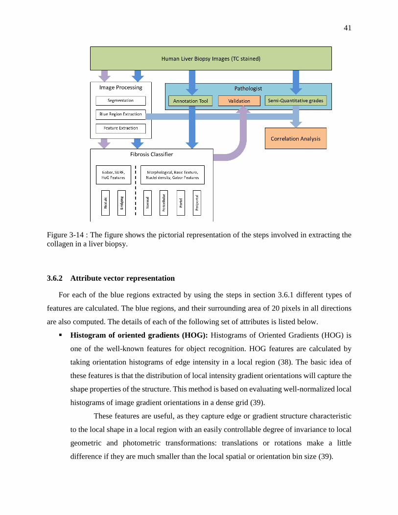
41

Figure 3-14 : The figure shows the pictorial representation of the steps involved in extracting the

collagen in a liver biopsy.

3.6.2 Attribute vector representation

For each of the blue regions extracted by using the steps in section 3.6.1 different types of

features are calculated. The blue regions, and their surrounding area of 20 pixels in all directions

are also computed. The details of each of the following set of attributes is listed below.

Histogram of oriented gradients (HOG): Histograms of Oriented Gradients (HOG) is

one of the well-known features for object recognition. HOG features are calculated by

taking orientation histograms of edge intensity in a local region (38). The basic idea of

these features is that the distribution of local intensity gradient orientations will capture the

shape properties of the structure. This method is based on evaluating well-normalized local

histograms of image gradient orientations in a dense grid (39).

These features are useful, as they capture edge or gradient structure characteristic

to the local shape in a local region with an easily controllable degree of invariance to local

geometric and photometric transformations: translations or rotations make a little

difference if they are much smaller than the local spatial or orientation bin size (39).

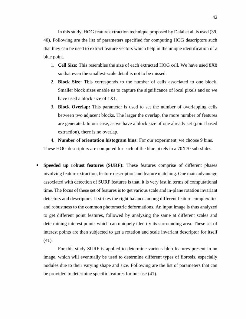
42

In this study, HOG feature extraction technique proposed by Dalal et al. is used (39,

40). Following are the list of parameters specified for computing HOG descriptors such

that they can be used to extract feature vectors which help in the unique identification of a

blue point.

1. Cell Size: This resembles the size of each extracted HOG cell. We have used 8X8

so that even the smallest-scale detail is not to be missed.

2. Block Size: This corresponds to the number of cells associated to one block.

Smaller block sizes enable us to capture the significance of local pixels and so we

have used a block size of 1X1.

3. Block Overlap: This parameter is used to set the number of overlapping cells

between two adjacent blocks. The larger the overlap, the more number of features

are generated. In our case, as we have a block size of one already set (point based

extraction), there is no overlap.

4. Number of orientation histogram bins: For our experiment, we choose 9 bins.

These HOG descriptors are computed for each of the blue pixels in a 70X70 sub-slides.

Speeded up robust features (SURF): These features comprise of different phases

involving feature extraction, feature description and feature matching. One main advantage

associated with detection of SURF features is that, it is very fast in terms of computational

time. The focus of these set of features is to get various scale and in-plane rotation invariant

detectors and descriptors. It strikes the right balance among different feature complexities

and robustness to the common photometric deformations. An input image is thus analyzed

to get different point features, followed by analyzing the same at different scales and

determining interest points which can uniquely identify its surrounding area. These set of

interest points are then subjected to get a rotation and scale invariant descriptor for itself

(41).

For this study SURF is applied to determine various blob features present in an

image, which will eventually be used to determine different types of fibrosis, especially

nodules due to their varying shape and size. Following are the list of parameters that can

be provided to determine specific features for our use (41).

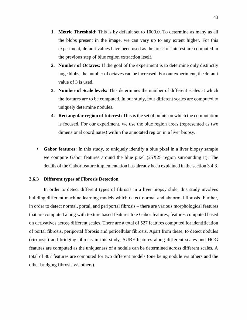
43

1. Metric Threshold: This is by default set to 1000.0. To determine as many as all

the blobs present in the image, we can vary up to any extent higher. For this

experiment, default values have been used as the areas of interest are computed in

the previous step of blue region extraction itself.

2. Number of Octaves: If the goal of the experiment is to determine only distinctly

huge blobs, the number of octaves can be increased. For our experiment, the default

value of 3 is used.

3. Number of Scale levels: This determines the number of different scales at which

the features are to be computed. In our study, four different scales are computed to

uniquely determine nodules.

4. Rectangular region of Interest: This is the set of points on which the computation

is focused. For our experiment, we use the blue region areas (represented as two

dimensional coordinates) within the annotated region in a liver biopsy.

Gabor features: In this study, to uniquely identify a blue pixel in a liver biopsy sample

we compute Gabor features around the blue pixel (25X25 region surrounding it). The

details of the Gabor feature implementation has already been explained in the section 3.4.3.

3.6.3 Different types of Fibrosis Detection

In order to detect different types of fibrosis in a liver biopsy slide, this study involves

building different machine learning models which detect normal and abnormal fibrosis. Further,

in order to detect normal, portal, and periportal fibrosis – there are various morphological features

that are computed along with texture based features like Gabor features, features computed based

on derivatives across different scales. There are a total of 527 features computed for identification

of portal fibrosis, periportal fibrosis and pericellular fibrosis. Apart from these, to detect nodules

(cirrhosis) and bridging fibrosis in this study, SURF features along different scales and HOG

features are computed as the uniqueness of a nodule can be determined across different scales. A

total of 307 features are computed for two different models (one being nodule v/s others and the

other bridging fibrosis v/s others).

44

3.6.4 Quantification of Collagen

Collagen accounts for the blue region present in a liver biopsy slide. Once the blue region

extraction is done, the amount of blue region is computed. The expert pathologists provide semi-

quantitative grades for each of the validation slides, based on the collagen content and the nature

of fibrosis present in a liver biopsy. In this study, the expert pathologists’ grades are quantified

with the amount of collagen content (blue region area computed) basing on the weighted average

sum of the blue region area to that of the tissue area.

45

4. RESULTS

This section involves the different results associated with the detection of steatosis,

inflammation and fibrosis and its types. In this study, quantification of each of the different

detected histological features are also studied and correlated by the expert pathologist grades.

Validation Metrics

There are various kinds of metrics that can be used to uniquely validate a supervised machine

learning classifier. In this study, we use the following different validation metrics.

Confusion Matrix:

Confusion matrix is a layout used to describe the performance of a classification

model. It contains the information about actual and classified data. It is a square matrix of

order n where n is the number of classes with rows having the predicted classes and the

columns having the actual classes. The following table gives an insight about the confusion

matrix of order 2.(42)

Table 4-1 : Confusion matrix of order 2.

Predicted

negative

Predicted positive

Actual negative a b

Actual positive c d

a is the number of true negative predictions which is the number of classes correctly

classified as negative.

b is the number of false positive predictions which is the number of classes incorrectly

classified as positive.

c is the number of false negative predictions which is the number of classes incorrectly

classified as negative.

d is the number of true positive predictions which is the number of classes correctly

classified as positive.

46

Precision (p):

Precision is the proportion of correct positive classifications from the samples that

are predicted as positive. In this case it measures the percentage of images correctly

identified as having the disease among all the images identified as having the disease.

By using the above example of confusion matrix, precision is calculated as follows

𝑝𝑟𝑒𝑐𝑖𝑠𝑖𝑜𝑛 = 𝑡𝑟𝑢𝑒 𝑝𝑜𝑠𝑖𝑡𝑖𝑣𝑒

𝑡𝑟𝑢𝑒 𝑝𝑜𝑠𝑖𝑡𝑖𝑣𝑒 + 𝑓𝑎𝑙𝑠𝑒 𝑝𝑜𝑠𝑖𝑡𝑖𝑣𝑒=

𝑑

𝑑 + 𝑏

Recall (r):

Recall is the ratio of the number of positive samples predicted as positive to the

actual number of positive samples. In our case it measures the proportion of actual images

with disease among the images identified as having disease.

𝑟𝑒𝑐𝑎𝑙𝑙 = 𝑡𝑟𝑢𝑒 𝑝𝑜𝑠𝑖𝑡𝑖𝑣𝑒

𝑡𝑟𝑢𝑒 𝑝𝑜𝑠𝑖𝑡𝑖𝑣𝑒 + 𝑓𝑎𝑙𝑠𝑒 𝑛𝑒𝑔𝑎𝑡𝑖𝑣𝑒=

𝑑

𝑑 + 𝑐

Receiver Operating Characteristic (ROC):

ROC is a graph plotted between True Positive Rate (also known as Recall) on Y

axis against False Positive Rate on X axis. It depicts the relative tradeoffs between benefits

(true positives) and costs (false positives) at various threshold settings.

False positive rate is the ratio of the number of samples which are predicted incorrectly to

the actual number of negative samples. From the above example of confusion matrix, False

Positive Rate is calculated as follows -

𝐹𝑎𝑙𝑠𝑒 𝑃𝑜𝑠𝑖𝑡𝑖𝑣𝑒 𝑅𝑎𝑡𝑒 = 𝑏

𝑏 + 𝑎

Each point plotted in ROC is an ordered pair of Recall and False Positive Rate. A classifier

has better performance characteristics if the curve is towards the upper left and close to X

axis since it results in high value of Recall (43).

47

Accuracy:

Classification accuracy is defined as the proportion of correct classifications among

all classifications. It is calculated as the ratio of the sum of number of true positives and

true negatives to the total number of samples.

From the above example of confusion matrix, the accuracy is

𝐴𝑐𝑐𝑢𝑟𝑎𝑐𝑦 = 𝑎 + 𝑑

𝑎 + 𝑏 + 𝑐 + 𝑑

F measure:

F1 score is the harmonic mean of Precision and Recall. It is a measure of accuracy

of a classifier. High F measure indicates the best performance as both the precision and

recall of the system are high.

𝐹1 𝑠𝑐𝑜𝑟𝑒 = 2 ∗ 𝑝 ∗ 𝑟

𝑝 + 𝑟

Correlation:

Correlation defines the strength of association between two continuous variables.

It is measured by a value called Correlation coefficient whose value typically lies between

-1 and +1. The closer the value of coefficient to either -1 or +1 the stronger is the relation

between both variables. Positive coefficient value indicates the directly proportional

relation whereas the negative correlation value indicates the inversely proportional relation

between the variables.

Pearson Correlation Coefficient:

It is the ratio of the covariance of two variables to their product of the standard

deviation where covariance of two variables is the expected value of the product of their

derivations from their individual expected values. This coefficient gives more accurate

values if the variables are normally distributed.

𝑟 = ∑ (𝑥𝑖 − 𝑥𝑚

𝑛𝑖=1 )(𝑦𝑖 − 𝑦𝑚)

√∑ (𝑥𝑖 − 𝑥𝑚)2𝑛𝑖=1 ∗ ∑ (𝑦𝑖 − 𝑦𝑚)2𝑛

𝑖=1

𝑥𝑖 and 𝑦𝑖 are the individual values of variables x and y respectively.

𝑥𝑚 and 𝑦𝑚 are the expected values (mean) of x and y respectively (44).

48

Spearman Correlation Coefficient:

Unlike the Pearson’s Coefficient, this coefficient does not assume that the variables

are normally distributed. It defines the strength of monotonic relationship between two

variables. The variables must be monotonically increasing or decreasing (If one variables

increases, the second variable should never decrease and vice-versa) and not necessarily

linear. It is obtained by performing Pearson Correlation Coefficient on the ranked variables.

Ranking is done by assigning the lowest value of 1 and the next lowest 2 and so on.

𝑟𝑠 = 1 −∑ 𝑑𝑖

2𝑛𝑖=1

𝑛(𝑛2 − 1)

𝑑𝑖 is the difference in ranks of x and y

n is the number of samples of x and y

Steatosis

I. Training Data

The training data for learning the macrosteatosis model is the white regions

annotated by Dr. C, including 2256 macrosteatosis annotations from 11 liver biopsy

images. The training data for learning the microsteatosis model was polygonal regions

annotated as microsteatosis by Dr. C, including 570 microsteatosis annotations from 5 liver

biopsy images.

II. Test Data

The test data to detect macrosteatosis comprises of 27 slides which provided with

semi-quantitative grades given by Dr. C. The test data to detect microsteatosis comprises

of 11 slides. These slides are processed and a random set of 10 sub-slides each identified

as microsteatosis by the built classifier are validated by Dr. C.

III. Detection and quantification results

In this study, the supervised machine learning models built to detect macrosteatosis

and microsteatosis are subjected to 10-fold cross validation. The training data comprised

of the annotated data given by the expert pathologists. All the present white regions could

not be used for the building of this model as it involved a lot of overlapped annotations.

49

For the macrosteatosis model, sinusoids and micro fat labels were not taken into

consideration because their annotations had a few overlaps with the other set of white

region classes and also, sinusoids were not extracted accurately during the white region

extraction because they are very tiny set of white regions and may be ignored during the

thresholding.

For the microsteatosis model, it consisted of only two classes namely,

microsteatosis regions and non-microsteatosis regions. The non-microsteatosis regions

comprise of all the other white region areas mentioned in the Table 4-2. Because of the

irregularity/imbalance associated with the number of annotations (568 micro fat, 2296

macro fat, 117 central vein, 121 bile duct, 75 portal vein and 22 portal artery), a random

subset of annotated data are removed and the rest is used for training. The feature extraction

is done pixel-wise and therefore, we randomly subsample 0.02% of the microsteatosis data

and 0.001% of any other white region extracted feature. Evaluation of accuracy of macro-

and microsteatosis identification was performed using a 10-fold cross validation in the

training set. For macrosteatosis prediction, the model’s precision, recall (sensitivity) and

area under the receiver operator characteristic (AUROC) were 94.2%, 95%, 99.1%,

respectively. The classifier’s accuracy was 84.2%.

When correlated with the pathologist’s semi-quantitative grade of macrosteatosis,

the model fits with a coefficient of determination 𝑅2 value of 0.905. Figure 4-1 shows the

2𝑛𝑑 order polynomial curve fitted to the data points. The strong correlation between

quantitative results obtained by the algorithm developed in this study for estimating the

percentage macrosteatosis and the pathologist macrosteatosis grades are shown in

Figure 4-2 (p=0.01 after performing two-sample t-test with a degree of freedom of 26).

Table 4-2 shows the confusion matrix of the model built for macrosteatosis prediction.

50

Table 4-2 : The confusion matrix and metrics for the model built to detect macrosteatosis.

For microsteatosis prediction, the model’s precision, recall and AUROC were

79.2%, 77%, 78.1%, respectively. The classifier’s accuracy was 78.7%. Table 4-3 shows

the confusion matrix of the model built for microsteatosis prediction.

Table 4-3 : The confusion matrix and metrics for the model built to detect microsteatosis.

Actual Predicted

Micro Fat Others PRECISION (%)

Micro Fat 7109 1862 79.24

Others 2116 7660 78.35

RECALL (%) 77.06 80.445

Figure 4-3 presents a visual summary of the performance metrics for the different

steatosis identification models developed using supervised machine learning methods

described above.

Actual Predicted

Central

Vein

Macro

Fat

Bile

Duct

Portal

Vein

Portal

Artery

PRECISION

(%)

Central Vein 230 8 0 25 0 87.45

Macro Fat 6 343 0 12 0 95.01

Bile Duct 0 1 17 27 5 30.91

Portal Vein 15 8 14 298 2 87.9

Portal Artery 2 4 4 7 13 37.14

RECALL

(%) 90.91 94.23 41.46 79.25 52

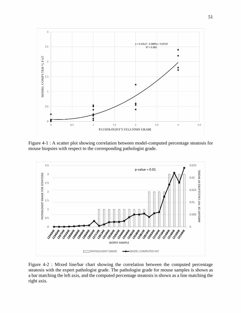
51

Figure 4-1 : A scatter plot showing correlation between model-computed percentage steatosis for

mouse biopsies with respect to the corresponding pathologist grade.

Figure 4-2 : Mixed line/bar chart showing the correlation between the computed percentage

steatosis with the expert pathologist grade. The pathologist grade for mouse samples is shown as

a bar matching the left axis, and the computed percentage steatosis is shown as a line matching the

right axis.

52

Figure 4-3 : A graph which represents the different steatosis models generated and their respective

metrics.

The expert pathologist validated the classification results on unseen slides for

detection of steatosis. For macrosteatosis, evaluation by the study expert pathologist of the

accuracy of predictions made on biopsy samples images unseen previously by the classifier,

showed 100% accuracy. For microsteatosis, of the one hundred and ten random sub slides

the detection accuracy was 63%. The pathologist also confirmed that for every unseen slide,

the classifier had accurately detected microsteatosis on at least one sub slide (i.e., 100%

sensitivity for detecting any microsteatosis). It is practically impossible for the pathologist

to label the massive number of macro- or microsteatosis lesions present on an individual

slide, but the classifier can do that automatically. Here we show examples in Figure 4-4

(for macrosteatosis) and Figure 4-5 (for microsteatosis), where both the pathologist’s and

classifier’s labels fell on the same lesion in the hepatocytes but the classifier correctly

labeled many other lesions in the same area of the biopsy. Figure 4-6 shows an example of

misclassified microsteatosis.

Other histological features of fatty liver such as lobular inflammation or ballooning,

or artifacts on the slides did not affect the performance of the model for detection of

macrosteatosis, as evidenced by the 100% accuracy of the classifier. However, they did for

microsteatosis, where ballooning or artifact was confused by the classifier as microsteatosis

in some mislabeled cases by the classifier (Figure 4-6).

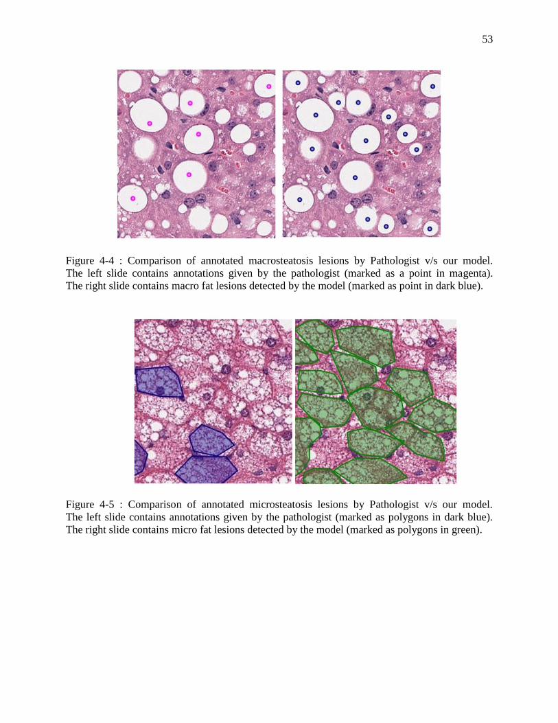
53

Figure 4-4 : Comparison of annotated macrosteatosis lesions by Pathologist v/s our model.

The left slide contains annotations given by the pathologist (marked as a point in magenta).

The right slide contains macro fat lesions detected by the model (marked as point in dark blue).

Figure 4-5 : Comparison of annotated microsteatosis lesions by Pathologist v/s our model.

The left slide contains annotations given by the pathologist (marked as polygons in dark blue).

The right slide contains micro fat lesions detected by the model (marked as polygons in green).

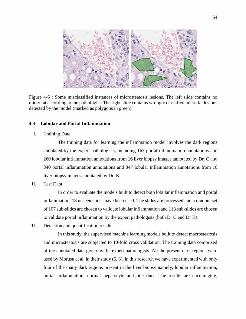
54

Figure 4-6 : Some misclassified instances of microsteatosis lesions. The left slide contains no

micro fat according to the pathologist. The right slide contains wrongly classified micro fat lesions

detected by the model (marked as polygons in green).

Lobular and Portal Inflammation

I. Training Data

The training data for learning the inflammation model involves the dark regions

annotated by the expert pathologists, including 163 portal inflammation annotations and

260 lobular inflammation annotations from 16 liver biopsy images annotated by Dr. C and

340 portal inflammation annotations and 347 lobular inflammation annotations from 16

liver biopsy images annotated by Dr. K.

II. Test Data

In order to evaluate the models built to detect both lobular inflammation and portal

inflammation, 18 unseen slides have been used. The slides are processed and a random set

of 107 sub-slides are chosen to validate lobular inflammation and 113 sub-slides are chosen

to validate portal inflammation by the expert pathologists (both Dr C and Dr K).


In this study, the supervised machine learning models built to detect macrosteatosis

and microsteatosis are subjected to 10-fold cross validation. The training data comprised

of the annotated data given by the expert pathologists. All the present dark regions were

used by Morusu et al. in their study (5, 6), in this research we have experimented with only

four of the many dark regions present in the liver biopsy namely, lobular inflammation,

portal inflammation, normal hepatocyte and bile duct. The results are encouraging,

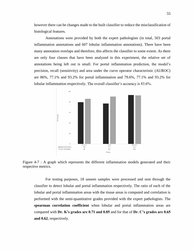
55

however there can be changes made to the built classifier to reduce the misclassification of

histological features.

Annotations were provided by both the expert pathologists (in total, 503 portal

inflammation annotations and 607 lobular inflammation annotations). There have been

many annotation overlaps and therefore, this affects the classifier to some extent. As there

are only four classes that have been analyzed in this experiment, the relative set of

annotations being left out is small. For portal inflammation prediction, the model’s

precision, recall (sensitivity) and area under the curve operator characteristic (AUROC)

are 86%, 77.1% and 93.2% for portal inflammation and 79.6%, 77.1% and 93.2% for

lobular inflammation respectively. The overall classifier’s accuracy is 83.6%.

Figure 4-7 : A graph which represents the different inflammation models generated and their

respective metrics.

For testing purposes, 18 unseen samples were processed and sent through the

classifier to detect lobular and portal inflammation respectively. The ratio of each of the

lobular and portal inflammation areas with the tissue areas is computed and correlation is

performed with the semi-quantitative grades provided with the expert pathologists. The

spearman correlation coefficient when lobular and portal inflammation areas are

compared with Dr. K’s grades are 0.71 and 0.85 and for that of Dr. C’s grades are 0.65

and 0.62, respectively.

56

Actual Predicted

Lobular

Inflammation

Normal

Hepatocyte

Portal

Inflammation

Bile

Duct

PRECISION

(%)

Lobular

Inflammation

4297 3 1206 64 79.6

Normal

Hepatocyte

21 88 0 0 76.5

Portal

Inflammation

914 24 9804 106 86.0

Bile Duct 165 0 396 552 76.5

RECALL

(%)

79.6 76.5 86.0 76.5


inflammation for human biopsies with respect to the corresponding Dr K’s grade.

y = 0.8442ln(x) + 5.0677

0

0.5

1

1.5

2

2.5

3

0 0.01 0.02 0.03 0.04 0.05 0.06 0.07

Pat

ho

logi

st G

rad

e

Model Prediction Grade

Portal Inflammation

Table 4-4 : The confusion matrix and metrics for the model built to detect inflammation.

57


inflammation for human biopsies with respect to the corresponding Dr K’s grade.


inflammation for human biopsies with respect to the corresponding Dr C’s grade.

y = 2.0089ln(x) + 8.6894

0

0.5

1

1.5

2

2.5

3

3.5

0 0.01 0.02 0.03 0.04 0.05 0.06 0.07

Pat

ho

logi

st G

rad

e


Lobular Inflammation

y = 0.6088ln(x) + 3.5756

0

0.5

1

1.5

2

2.5

0 0.01 0.02 0.03 0.04 0.05 0.06 0.07

Pat

ho

logi

st G

rad

e


Portal Inflammation

58


inflammation for human biopsies with respect to the corresponding Dr C’s grade.


inflammation for human biopsies with respect to the average of Dr C and Dr K’s pathologist grade.

y = 1.2692ln(x) + 5.8024

0

0.5

1

1.5

2

2.5

3

3.5

0 0.01 0.02 0.03 0.04 0.05 0.06 0.07

Pat

ho

logi

st G

rad

e



y = 0.6809ln(x) + 4.0852

0

0.5

1

1.5

2

2.5

0 0.01 0.02 0.03 0.04 0.05 0.06 0.07

Pat

ho

logi

st G

rad

e


Portal Inflammation

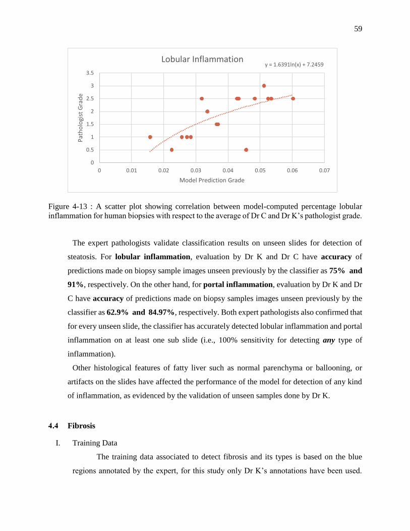
59


inflammation for human biopsies with respect to the average of Dr C and Dr K’s pathologist grade.

The expert pathologists validate classification results on unseen slides for detection of

steatosis. For lobular inflammation, evaluation by Dr K and Dr C have accuracy of

predictions made on biopsy sample images unseen previously by the classifier as 75% and

91%, respectively. On the other hand, for portal inflammation, evaluation by Dr K and Dr

C have accuracy of predictions made on biopsy samples images unseen previously by the

classifier as 62.9% and 84.97%, respectively. Both expert pathologists also confirmed that

for every unseen slide, the classifier has accurately detected lobular inflammation and portal

inflammation on at least one sub slide (i.e., 100% sensitivity for detecting any type of

inflammation).

Other histological features of fatty liver such as normal parenchyma or ballooning, or

artifacts on the slides have affected the performance of the model for detection of any kind

of inflammation, as evidenced by the validation of unseen samples done by Dr K.

Fibrosis

I. Training Data

The training data associated to detect fibrosis and its types is based on the blue

regions annotated by the expert, for this study only Dr K’s annotations have been used.

y = 1.6391ln(x) + 7.2459

0

0.5

1

1.5

2

2.5

3

3.5

0 0.01 0.02 0.03 0.04 0.05 0.06 0.07

Pat

ho

logi

st G

rad

e



60

Dr.C’s annotations are present for some types of fibrosis but not all, hence they have not

been used as part of this study. Dr. K has annotated blue regions, including 186 normal

fibrosis annotations, 118 portal fibrosis annotations, 128 pericellular annotations, 127

periportal annotations, 98 bridging annotations and 61 nodule annotations from a set of 18

liver biopsy images.

II. Test Data

The test data to detect the blue regions i.e. the amount of collagen content comprises

of 18 liver biopsy TC stained slides which are semi-quantitively graded by both the expert

pathologists.


In this study, the supervised machine learning models built to detect if a patient is

affected by abnormal fibrosis and also detect the different types of fibrosis associated are

subjected to 10-fold cross validation. The training data comprised of the annotated data

given by the expert pathologists. All the present blue regions could not be used for the

building of the models which were used to detect fibrosis and its types as it involved a lot

of overlapped annotations. This is one of the prime reasons for the detection results to be

comparatively low compared to that of steatosis and inflammation detection. The Figure

4-14 gives an example of blue region extraction using the method described above in

Section 3.6.1.

Figure 4-14 : An example of blue region detection in a TC Stained sub-slide.

A) A TC Stained sub-slide. B) Blue regions in the TC Stained sub-slide.

61

The first experiment conducted involves quantification of the collagen content in

liver biopsies and correlating the same with the semi-quantitative grades of the experts.

The amount of collagen content is detected by calculating the blue region areas and

performing a weighted averages sum of the pixel values in the blue band and thus, taking

the ratio of the blue region area with the tissue area. The conclusion of this study is that

even though there can be loads of collagen content in a liver biopsy, it need not necessarily

imply that the patient is highly affected with fibrosis. For this experiment, a total of 18

slides were processed and the percentage of collagen in each of them is computed. The

coefficient of determination of collagen area with Dr. K’s grades is 0.607 and with Dr. C’s

grades is 0.867. Hence, it is important to categorize the type of fibrosis associated in a liver

biopsy to determine at what extent a person is affected with NAFLD.

Figure 4-15 : A scatter plot showing correlation between model-computed percentage collagen

content for human biopsies with respect to the Dr K’s pathologist grade.

y = 73.031x2 + 10.28x - 0.7224R² = 0.6071

-0.5

0

0.5

1

1.5

2

2.5

3

3.5

4

4.5

0 0.05 0.1 0.15 0.2

Fibrosis Collagen content - Correlation with Dr K

62

Figure 4-16 : A scatter plot showing correlation between model-computed percentage collagen

content for human biopsies with respect to the Dr C’s pathologist grade.

Figure 4-17 : A bar graph which shows semi-quantitative grades given by both Dr. K and

Dr. C for the given test set of 17 human liver slides.

y = 310.57x2 - 44.386x + 1.4567R² = 0.867

-0.5

0

0.5

1

1.5

2

2.5

3

3.5

4

4.5

0 0.05 0.1 0.15 0.2

Fibrosis Collagen content - Correlation with Dr C

-1

0

1

2

3

4

5

1 2 3 4 5 6 7 8 9 10 11 12 13 14 15 16 17 18

Fibrosis Grade_Dr K Fibrosis Grade_Dr C

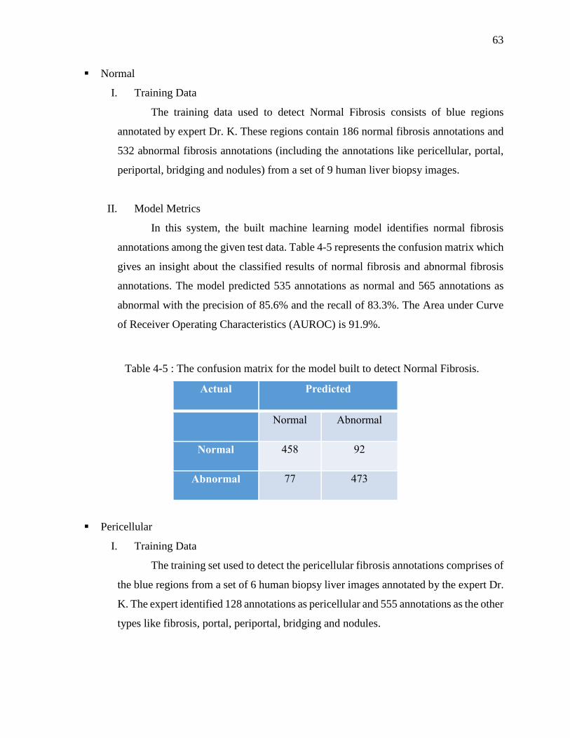
63

Normal

I. Training Data

The training data used to detect Normal Fibrosis consists of blue regions

annotated by expert Dr. K. These regions contain 186 normal fibrosis annotations and

532 abnormal fibrosis annotations (including the annotations like pericellular, portal,

periportal, bridging and nodules) from a set of 9 human liver biopsy images.

II. Model Metrics

In this system, the built machine learning model identifies normal fibrosis

annotations among the given test data. Table 4-5 represents the confusion matrix which

gives an insight about the classified results of normal fibrosis and abnormal fibrosis

annotations. The model predicted 535 annotations as normal and 565 annotations as

abnormal with the precision of 85.6% and the recall of 83.3%. The Area under Curve

of Receiver Operating Characteristics (AUROC) is 91.9%.

Table 4-5 : The confusion matrix for the model built to detect Normal Fibrosis.

Actual Predicted

Normal Abnormal

Normal 458 92

Abnormal 77 473

Pericellular

I. Training Data

The training set used to detect the pericellular fibrosis annotations comprises of

the blue regions from a set of 6 human biopsy liver images annotated by the expert Dr.

K. The expert identified 128 annotations as pericellular and 555 annotations as the other

types like fibrosis, portal, periportal, bridging and nodules.

64

II. Model Metrics

In this system, the model predicted 137 annotations as pericellular and 115

annotations as others from the Test Data. The classified annotations by the model are

shown in the confusion matrix represented by the table 4-6. The precision of the

classification model is 76.6% and the recall is 82.7%.

Table 4-6 : The confusion matrix for the model built to detect Pericellular Fibrosis.

Actual Predicted

Pericellular Others

Pericellular 105 22

Others 32 93

Portal

I. Training Data

The training set used to identify the portal fibrosis annotations comprises of

blue regions classified as 118 portal annotations and 565 other annotations (like

normal, pericellular, periportal, bridging and nodules) from a set of 6 human liver

biopsy images by the expert Dr. K.

II. Model Metrics

The model classified the test data as 365 portal annotations and 293 other

annotations with a precision of 77% and a recall of 84.4%. The comparison between

the actual and predicted annotation results is shown in the confusion matrix

represented by the table 4-7.

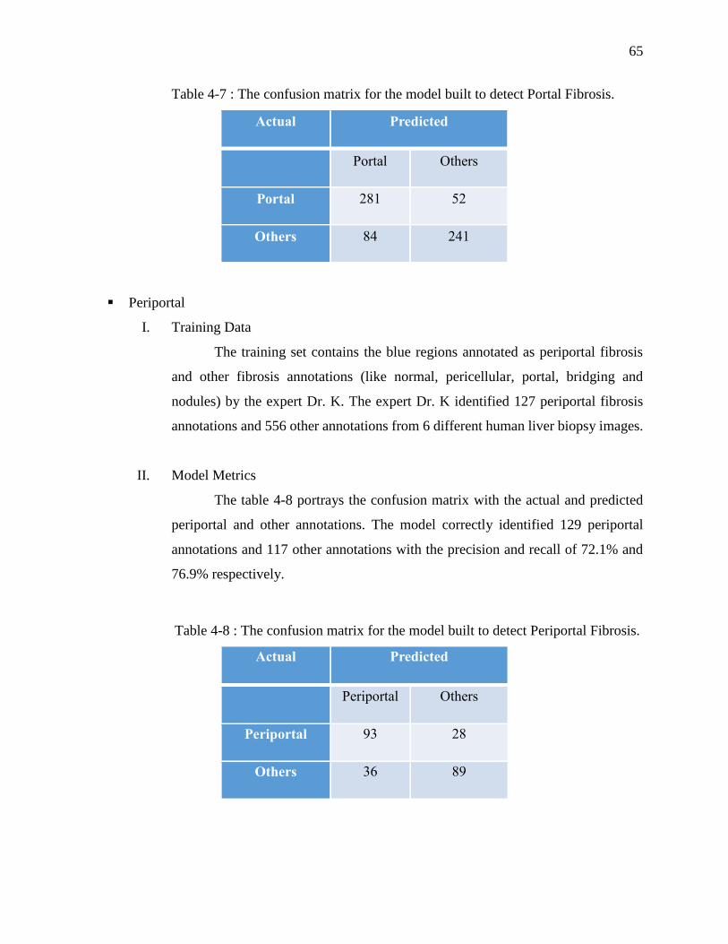
65

Table 4-7 : The confusion matrix for the model built to detect Portal Fibrosis.

Actual Predicted

Portal Others

Portal 281 52

Others 84 241

Periportal

I. Training Data

The training set contains the blue regions annotated as periportal fibrosis

and other fibrosis annotations (like normal, pericellular, portal, bridging and

nodules) by the expert Dr. K. The expert Dr. K identified 127 periportal fibrosis

annotations and 556 other annotations from 6 different human liver biopsy images.

II. Model Metrics

The table 4-8 portrays the confusion matrix with the actual and predicted

periportal and other annotations. The model correctly identified 129 periportal

annotations and 117 other annotations with the precision and recall of 72.1% and

76.9% respectively.

Table 4-8 : The confusion matrix for the model built to detect Periportal Fibrosis.

Actual Predicted

Periportal Others

Periportal 93 28

Others 36 89

66

Bridging

I. Training Data

The training set used to identify bridging fibrosis annotations is selected

across 9 human liver biopsy images by the expert Dr. K. The annotations contain

98 bridging fibrosis and 620 other fibrosis (like normal, pericellular, portal,

periportal and nodules).

II. Model Metrics

The classification results are interpreted as a confusion matrix shown in the

table 4-9. The model predicted 2159 bridging fibrosis annotations with a precision

of 84.9% and a recall of 91.7%.

Table 4-9 : The confusion matrix for the model built to detect Bridging Fibrosis.

Actual Predicted

Bridging Others

Bridging 1833 167

Others 326 1674

Nodule

III. Training Data

The training set used to predict the nodule fibrosis annotations is selected

from a set of 9 human liver biopsy images. The expert Dr. K annotated the input

images into a total of 61 nodules and 657 other fibrosis annotations (including

normal, pericellular, portal, periportal and bridging annotations).

IV. Model Metrics

The model predicted 2040 annotations as nodules and 1960 annotations.

The precision of the learning model is 89.8% and the recall is 91.6%. The confusion

matrix with correct and incorrect classification is presented in the table 4-10.

67

Table 4-10 : The confusion matrix for the model built to detect Nodule Fibrosis.

Actual Predicted

Nodules Others

Nodules 1831 169

Others 209 1791

For the detection of normal fibrosis in liver biopsies, a model is built with two

classes – normal fibrosis and abnormal fibrosis which comprises of a random subset of all

the different kinds of fibrosis respectively. The model thus built contains a total of 528

features which comprise of different set of morphological features, scaled representation

features and Gabor features (as discussed previously). Because of the irregularity of the

annotations, random subsampling takes place to fill the abnormal fibrosis class to avoid

overfitting of the model (886 normal fibrosis and 990 abnormal fibrosis). Feature extraction

is done using information gain such that the top 200 attributes are chosen to build the model.

There are two models built for the normal fibrosis detection, one with all the attributes and

the other with top 200 attributes. The best results obtained were with the former which

recorded a precision, recall and area under ROC (AUROC) characteristic curve of 85%,

79.5% and 90.5% respectively.

In order to detect the different other types of fibrosis, morphological features,

scaled representation features and Gabor features are computed for the annotated areas by

Dr K and individual models are built for all the five types of fibrosis. The models thus built

using the above methods described detect portal fibrosis, periportal fibrosis and pericellular

fibrosis with a precision of 77%, 72.1% and 76.6% respectively. However the model did

not give significant results for the detection of bridging fibrosis and cirrhosis.

The next two experimental models built involve detection of bridging fibrosis and

cirrhosis. Cirrhosis involves detection of nodules in a liver biopsy. These are oval shaped

hollow blue regions of different sizes. Therefore, detection of SURF features at different

scales will determine them to be unique as at the highest possible scale, the elliptical shape

hollow nodule collapses to a point. In the case of bridging fibrosis, there can be other types

68

of fibrosis within them. Hence, to capture the stream of blue regions across the tissue areas,

HOG descriptors are useful. Therefore, to detect the above two mentioned types of fibrosis,

texture features, HOG descriptors and SURF features across different scales are computed

and two class models involving nodules and others (a random subsampling of the other set

of fibrosis types) as well as bridging fibrosis and others is built. There are a total number

of 305 features that are computed which uniquely determine a blue region. The model

results for detection of bridging fibrosis and nodules have a precision of 84.9% and 89.8%,

respectively.

There are a lot of overlaps present in the given annotations for each type of fibrosis.

The use of square annotations to annotate this kind of fibrosis is something which needs to

be re-evaluated in the future. Some scope of improvements can be done if the annotations

are provided in a little more accurate way, thereby reducing the conflict of two different

types of fibrosis in the same region.

Table 4-11 : The different types of fibrosis detection with their respective precisions.

FIBROSIS TYPE PRECISION

Normal 85.6%

Pericellular 76.6%

Portal 77%

Periportal 72.1%

Bridging 84.9%

Cirrhosis 89.8%

69

5. DISCUSSION

The results presented above indicate that it is feasible to construct a decision support

system for pathologists who diagnose NAFLD using a supervised machine learning approach. The

use of such a system would minimize the variability and subjectivity present in the current semi-

quantitative grading system.

Pathologists can have a difference of opinion while scoring a liver biopsy slide for NAFLD,

which is one of the main motivations to the research presented in this thesis. The pathologists

involved in this study are well respected and experts in their field, however, the manual semi-

quantitative grading system is prone to subjectivity and variability. This has been indicated in our

study. The correlation with the pathologist grade is an important statistic, but it is also important

to consider the overall accuracy of the various classifiers built. The correlation with pathologist

grade is significant based on the underlying assumption that the pathologist is 100% correct. Over

a period of time, there is a possibility of considering this type of continuous assessment for the

detection of NAFLD thereby, eliminating the use of pathologist semi-quantitative grades.

The classifiers built to detect different types of fibrosis can have better accuracies, ideally.

There are a few points which could enhance the above set of models. Firstly, the annotations used

to build fibrosis classifiers contain many overlaps. This can be improved by the introduction of

new set of markers for each type of fibrosis. Secondly, the pathologists' disagreement on semi-

quantitative grades indicate that the correlation analysis performed on each their scores yield better

results as compared to pathologist to pathologist correlation. The inclusion of many number of

pathologists could help building widely accepted classifiers and eliminate variability. Thirdly, the

use of random subset of slides for validation can be subject to unevenness i.e. there is a possibility

that some of the randomly chosen sub-slides can in fact belong to the negative class.

Finally, performance of this type of system is very important while introducing it in a

clinical setting. The current execution time is not very efficient, as tools like MATLAB, WEKA

used to develop these classifiers are very good for prototyping. The use of a programming language

which could efficiently utilize system resources could make this process faster compared to the

current system.

70

6. CONCLUSION

The above section elaborates on the promising results for determining various histological

features in liver biopsies (both mice and human) which can help detect NAFLD. The use of various

image processing techniques involved to generate unique set of features which are then used to

build supervised machine learning models is therefore, a unique and more accurate measure of

detecting different anatomical and histological features in biopsies as there can be enumerable

number of slides and it becomes tough for a pathologist to not miss any of them. Hence, it also

reduces the inter-observer and intra-observer error associated while performing the semi-

quantitative assessment by the pathologists.

For all our experimental studies conducted, we receive the annotations and the semi-

quantitative grades from the expert pathologists who are considered the “gold standard” in the field

of histopathology. Despite the fact the pathologists are one of the best in their areas, there is a

definite disagreement between them while grading slides. This clearly accounts to our process of

quantification and detection of different histological set of features, which would be very

beneficial for the doctors in the field of Hepatology and Pathology. This tool has been built to

serve as a utility to the doctors and not to replace their existence.

The improvements done to the models which determine the steatosis area in a liver biopsy

clearly indicate that this tool is “ready for use” in clinical trials for detecting macrosteatosis and

microsteatosis as mentioned by Morusu et al. in their study (5, 6). Apart from this, the encouraging

results for detection of both the types of inflammation indicate that with more improvements put

in place, this tool can be used soon by doctors in their clinical trials. In this study, the addition of

detecting collagen in liver biopsies and also categorizing the different types of fibrosis in a liver

biopsy is a step in the right direction to build a fully automated tool to detect NAFLD in mice and

humans.

The current constraint for this tool however lies in the fact that, it takes time to evaluate

the above mentioned histological features. Having said that, improvements have been made to

make it a speedy robust system and running the same using various big data technologies should

be a boost as we move forward.

71

REFERENCES

1. Kleiner DE, Brunt EM, Natta MV, Behling C, Contos MJ, Cummings OW, et al. Design

and validation of a histological scoring system for nonalcoholic fatty liver disease.

Hepatology. 2005;41(6):1313-21.

2. Younossi Z, Anstee QM, Marietti M, Hardy T, Henry L, Eslam M, et al. Global burden of

NAFLD and NASH: trends, predictions, risk factors and prevention. Nature Reviews

Gastroenterology & Hepatology. 2017;15:11.

3. Younossi ZM, Stepanova M, Rafiq N, Makhlouf H, Younoszai Z, Agrawal R, et al.

Pathologic criteria for nonalcoholic steatohepatitis: Interprotocol agreement and ability to

predict liver‐related mortality. Hepatology. 2011;53(6):1874-82.

4. Pournik O, Alavian SM, Ghalichi L, Seifizarei B, Mehrnoush L, Aslani A, et al. Inter-

observer and Intra-observer Agreement in Pathological Evaluation of Non-alcoholic Fatty

Liver Disease Suspected Liver Biopsies. Hepatitis Monthly. 2014;14(1):e15167.

5. Morusu S, Tuceryan M, Kleiner D, W. Cummings O, Vanderbeck S, Chalasani N, et al.

Mo1564 Automated Method to Detect and Quantify Lobular Inflammation and Portal

Inflammation in Human Liver Biopsy Images. 2016.

6. Morusu S, Tuceryan M, W. Cummings O, Zhang H, Yin X-M, Vanderbeck S, et al. Sa1675

Automated Method to Detect and Quantify Macrovesicular Steatosis in Murine Fatty Liver.

2016.

7. Vanderbeck S, Bockhorst J, Kleiner D, Komorowski R, Chalasani N, Gawrieh S.

Automatic quantification of lobular inflammation and hepatocyte ballooning in NAFLD

liver biopsies. 2015.

8. Vanderbeck S, Bockhorst J, Komorowski R, E Kleiner D, Gawrieh S. Automatic

classification of white regions in liver biopsies by supervised machine Learning. 2013.

9. Vanderbeck S, Bockhorst J, Komorowski R, E. Kleiner D, Chalasani N, Gawrieh S. 926

Automatic Quantification of Liver Histology in NAFLD: A Promising Tool to Facilitate

Better Histological Characterization in NAFLD. 2014.

10. Reeder SB, Sirlin C. Quantification of Liver Fat with Magnetic Resonance Imaging.

Magnetic resonance imaging clinics of North America. 2010;18(3):337-57.

72

11. Morusu SP. Automated Methods to Detect and Quantify Histological Features in Liver

Biopsy Images to aid in the Diagnosis of Non-Alcoholic Fatty Liver Disease. [Thesis]:

Purdue University; 2016.

12. Abdel-Misih SRZ, Bloomston M. Liver Anatomy. The Surgical clinics of North America.

2010;90(4):643-53.

13. King D. Organization of Liver Lobules. Southern Illinois University: SIU School of

Medicine; 2010.

14. Sibulesky L. Normal liver anatomy. Clinical Liver Disease. 2013;2(S1):S1-S3.

15. Mitchell L. Shiffman MD. Liver Biopsy Website: National Institute of Diabetes and

Digestive and Kidney Diseases, National Institute of Health; 2014.

16. Takahashi Y, Fukusato T. Histopathology of nonalcoholic fatty liver disease/nonalcoholic

steatohepatitis. World Journal of Gastroenterology : WJG. 2014;20(42):15539-48.

17. Kleiner DE, Makhlouf HR. Histology of NAFLD and NASH in Adults and Children.

Clinics in liver disease. 2016;20(2):293-312.

18. Harmon RC, Tiniakos DG, Argo CK. Inflammation in nonalcoholic steatohepatitis. Expert

Review of Gastroenterology & Hepatology. 2011;5(2):189-200.

19. Ribeiro R, Marinho RT, Sanches JM, editors. Global and local detection of liver steatosis

from ultrasound. 2012 Annual International Conference of the IEEE Engineering in

Medicine and Biology Society; 2012 Aug. 28 2012-Sept. 1 2012.

20. Homeyer A. Fast and accurate identification of fat droplets in histological images.

Computer methods and programs in biomedicine. 2015;121(2):59-65.

21. Robinson MW, Harmon C, O’Farrelly C. Liver immunology and its role in inflammation

and homeostasis. Cellular & Molecular Immunology. 2016;13:267.

22. Masseroli M, Caballero T, O'Valle F, Moral RMGD, Pérez-Milena A, Moral RGD.

Automatic quantification of liver fibrosis: design and validation of a new image analysis

method: comparison with semi-quantitative indexes of fibrosis. Journal of

Hepatology.32(3):453-64.

23. Gamal MD, Mohamed MK, Hussein ME-B, Fouda A-MM, Osama ASE-D. Digital

quantification of fibrosis in liver biopsy sections: Description of a new method by

Photoshop software. Journal of Gastroenterology and Hepatology. 2004;19(1):78-85.

73

24. Dioguardi N, Franceschini B, Russo C, Grizzi F. Computer-aided morphometry of liver

inflammation in needle biopsies. World Journal of Gastroenterology. 2005;11(44):6995-

7000.

25. Institute NHGR. Why Mouse Matters The Forefront of Genomics: National Institute of

Health; 2000.

26. Ding WX, Li M, Chen X, Ni HM, Lin CW, Gao W, et al. Autophagy Reduces Acute

Ethanol-Induced Hepatotoxicity and Steatosis in Mice. Gastroenterology.

2010;139(5):1740-52.

27. Kleiner DE, Brunt EM, Van Natta M, Behling C, Contos MJ, Cummings OW, et al. Design

and validation of a histological scoring system for nonalcoholic fatty liver disease.

Hepatology. 2005;41(6):1313-21.

28. Tuceryan M, Jain AK. Texture Analysis. In: Chen CH, Pau LF, Wang PSP, editors. The

Handbook of Pattern Recognition and Computer Vision (2nd Edition): World Scientific

Publishing Co.; 1998. p. 207-48.

29. Clark M, Bovik AC, Geisler WS. Texture Segmentation Using Gabor Modulation

Demodulation. Pattern Recogn Lett. 1987;6(4):261-7.

30. Boukerroui D, Noble JA, Brady M. On the choice of band-pass quadrature filters. J Math

Imaging Vis. 2004;21(1):53-80.

31. Daugman JG. Complete Discrete 2-D Gabor Transforms by Neural Networks for Image-

Analysis and Compression. Ieee T Acoust Speech. 1988;36(7):1169-79.

32. Zhang L, Mistry K, Jiang M, Neoh SC, Hossain MA. Adaptive facial point detection and

emotion recognition for a humanoid robot. Comput Vis Image Und. 2015;140:93-114.

33. Petkov N. Biologically Motivated Computationally Intensive Approaches to Image

Pattern-Recognition. Future Gener Comp Sy. 1995;11(4-5):451-65.

34. Jain AK, Farrokhnia F. Unsupervised Texture Segmentation Using Gabor Filters. Pattern

Recogn. 1991;24(12):1167-86.

35. Vanderbeck S, Bockhorst J, Komorowski R, Kleiner DE, Gawrieh S. Automatic

classification of white regions in liver biopsies by supervised machine learning. Human

pathology. 2014;45(4):785-92.

36. Pratt WK. Digital Image Processing: PIKS Inside: John Wiley & Sons, Inc.; 2001.

74

37. Otsu N. A threshold selection method from gray-level histograms. IEEE transactions on

systems, man, and cybernetics. 1979;9(1):62-6.

38. Kobayashi T, Hidaka A, Kurita T, editors. Selection of Histograms of Oriented Gradients

Features for Pedestrian Detection. 2008; Berlin, Heidelberg: Springer Berlin Heidelberg.

39. Dalal N, Triggs B, editors. Histograms of oriented gradients for human detection. 2005

IEEE Computer Society Conference on Computer Vision and Pattern Recognition

(CVPR'05); 2005 25-25 June 2005.

40. Dalal N, Triggs B, editors. Histograms of oriented gradients for human detection.

Computer Vision and Pattern Recognition, 2005 CVPR 2005 IEEE Computer Society

Conference on; 2005 25-25 June 2005.

41. Bay H, Tuytelaars T, Van Gool L, editors. SURF: Speeded Up Robust Features. 2006;

Berlin, Heidelberg: Springer Berlin Heidelberg.

42. Visa S, Ramsay B, Ralescu A, Van Der Knaap E. Confusion Matrix-based Feature

Selection. MAICS. 2011.

43. Fawcett T. An introduction to ROC analysis. Pattern Recognition Letters. 2006;27(8):861-

74.

44. Mukaka MM. A guide to appropriate use of Correlation coefficient in medical research.

Malawi Medical Journal : The Journal of Medical Association of Malawi. 2012;24(3):69-

71.

detection of histological features in liver biopsy …

Documents