What you sequence What you see in the electropherogram

Gn

G+G2n

Gn

APPLICATION NOTE Sanger Sequencing Data Analysis

The introduction of semi-automated fluorescent dye-terminator DNA Sequencing using capillary electrophoresis (aka CE or Sanger sequencing) has revolutionized life and medical sciences by unraveling complete genomes and the elucidation of genetic structures of many organisms. The primary information and value of the DNA sequencing process is the identification of the nucleotides and of possible sequence variants. A largely unknown and unexplored feature of fluorescent Sanger sequencing traces is the quantitative information embedded therein. With the growing need for quantifying somatic mutations in tumor tissue, emerging mutations in viral genomes conferring drug resistance, or the amount of methylation in a particular CpG locus, it is desirable to exploit the potential of the quantitative information obtained from sequencing traces.

In this application note we review two freely available software applications that help to extract and present the peak height data

of Sanger sequencing traces for quantitative data analysis.

The composite electropherogram and the challenge of mixed basecallingDNA basecalling software programs analyze fluorescent Sanger sequencing traces and reveal the base identities of a DNA sample along with quality values (phred scores) which indicate the reliability of the basecall. In a typical PCR-based sequencing project that uses DNA from a diploid organism both copies of an allele are sequenced simultaneously. Compared to the hypothetical signal n resulting

Detection and Quantification of Sequence Variants from Sanger Sequencing TracesDetermination of minor alleles by analyzing peak height data

Figure 1: Homozygosity. The peak signal is the sum of the peak signals from the two haploid input DNAs.

from a single allele, the observed signal is actually the result of both alleles combined, or 2n.

An individual peak in a sequencing trace representing a homozygous base is a composite mixture of two identical bases each contributing approximately half of the fluorescent signal in relative fluorescent units (RFU) to a given peak height (see Figure 1). Hence, the loss (e.g., by amplification drop out) of one allele will typically lead to a drop of signal by half (illustrated in Figure 2).

In the case of heterozygosity at an allele the resulting peak pair migrates at the same or

2

similar position as a mixed base. The signal strength of each component is approximately half of the homozygous counterpart. Ideally, the two heterozygous peaks appear to be of equal height (see outcome I) but in reality they may occur somewhat unbalanced (outcome II or III) depending on the DNA strand sequenced and sequence-dependent context. This complicates the determination of peak height ratios. However, this imbalance phenomenon is typically highly reproducible for a given allele from sample to sample and can be

accounted for using homozygous control samples (see text). (Figure 3)

The simple principle that the proportion of each of two sequence variants in a mixture determine the relative heights of the peaks that represent each variant in a sequence electropherogram has inspired Ian Carr and colleagues from the University of Leeds Institute of Molecular Medicine to develop a software application that exploits the quantitative information embedded in a sequencing trace.

Homozygous and heterozygous sequence variants are readily

Figure 2: Allele Drop-Out. The peak signal is only approximately half of the signal expected in the case of homozygosity.

Figure 3: Heterozygosity: sequencing a heterozygous allele may ideally present in an electropherogram as a balanced peak pair (Outcome I) or may appear somewhat imbalanced (Outcome II or III). The specific outcome for a given peak pair is typically highly reproducible and depends on the local sequence context.

What you sequence What you see in the electropherogram

Gn

G“1n”

Gn

What you sequence What you see in the electropherogram

Gn

R (G+A)2n I

IIR (G+A)

2n

IIIR (G+A)

2n

An

detected by commercial and public domain sequence analysis software packages. However, minor sequence variants such as they are found in somatic mutations in tumor tissue or in emerging mutations in subpopulations of microbial or viral organisms often elude detection because the abundance of the minor allele is too low for triggering a (mixed) basecall.

The heights of the primary and secondary peaks in a mixed-base situation are the most important attributes for basecalling. If the peak height ratio of a secondary to a

3

primary peak drops below 30% (or other user-set threshold) it is usually not considered and therefore not called out as a mixed base.

In this application note we will review the paper and the QSVanalyzer software published by Ian Carr et al. from the University of Leeds, UK and recommend its utility for the detection and quantification of sequence variants.

We also describe a new bioinformatics utility, ab1PeakReporter, which is available on the Life Technologies web site. The utility provides numerical peak height data of Sanger sequencing traces allowing the quantitative analysis of peak height data. To that end, we show how minor alleles can be quantified by polynomial regression analysis using Microsoft Excel® software.

• Move .ab1 files for QSV analysis into a project folder

• Must include homozygous counterparts for (heterozygous) allele(s) of interest

• Open .ab1 file of sample with allele of interest

• Inspect electropherogram and

• Select peak(s) of interest and 5´ reference peaks

• Run Batch command and select project folder as input source

• QSV analysis is executed and a report folder with results is deposited in the project folder

• Open result folder “QSV Data” located in project folder

• Review results

• Optional: if calibrator files (dilution series) are included in data set use file “QSV_ratios.xls” as source for quantitation analysis by polynomial regression using Microsoft Excel® software LINEST function (See text and Figure 7)

Figure 4: Overview of the QSVanalyzer workflow.

Inferring Allelic Variant Ratios using QSVAnalyzerIn 2009, Carr et al. published a paper describing the QSVanalyzer desktop application in the journal Bioinformatics. QSVanalyzer enables the high-throughput quantification of the proportions of DNA sequences containing single-nucleotide sequence variants (SNVs) from fluorescent Sanger sequencing traces. The paper is open access and can be downloaded with supplementary data from [1]. The QSVanalyzer application including original sequencing trace files used in the study can be downloaded from http://dna.leeds.ac.uk/qsv/ .

In the paper, Carr et al. demonstrated the utility of the method for estimation of copy number proportions (CNPs) for various quantitative sequence variant (QSV) types such as common

regular SNPs, paralogous sequence variants (PSV) and SNPs in the background of copy number variation (CNV).

An important concept presented in the paper is the normalization of electropherograms: Fluorescent dideoxynucleotide terminators are incorporated dependent on their sequence context and may appear imbalanced in heterozygous mixed bases (see Figure 3). Further, the amount of template DNA and other factors affect the absolute peak height. Therefore, relative (rather than absolute) peak heights are determined by comparing the variant nucleotide’s peak height to that of an invariant nucleotide located 5’ (upstream) where one can assume a neutral sequence background, i.e., no variant–introduced effects. The software also corrects for the background baseline signal in each

4

Figure 5: Electropherogram viewer with a heterozygous allele “S (for C and G)” near scan # 900.

Figure 6: Output reports of the QSVanalyzer application. (A) Widget of the electropherogram accompanied by peak heights of the area. (B) Comprehensive Excel-readable table with raw and reference-adjusted data. (C) Final Quantitative Sequence Variant (QSV) report with adjusted peak heights (see Carr et al. for details).

A B

C

5

trace and subtracts the allele-specific “background noise” from the relative peak height for a final normalized peak height (NPH). To calculate the QSV ratio, the program needs two reference sequences, each containing the homozygous allele of the two variants.

A detailed, illustrated guide for use of the application can be found on http://dna.leeds.ac.uk/qsv/guide/ and a set of original .ab1 sample files with a differential dilution series is available on http://dna.leeds.ac.uk/qsv/download.

Figure 5 shows the electropherogram viewer with a heterozygous allele “S (for C and G)” near scan # 900 along with the QSV information setup window where this and other alleles of interest are selected for subsequent batch analysis of QSV ratios (step 2 of workflow).

Figure 6 shows QSVanalyzer results for a mixed DNA sample that contained a pre-mixed ratio of 40% variant A (C nucleotide blue trace) and 60% variant B (G nucleotide black trace). QSVanalyzer reported a ratio of 0.4 to 0.6 for A:B (see report 6C).

What is the limit of detection for minor alleles?The Carr paper provides a web link to sets of original sequencing files from three dilution series each consisting of 11 samples in triplicates with nominal sequence variant proportions 10:0, 9:1, 8:2, 7:3, 6:4, 5:5, 4:6, 3:7, 2:8, 1:9, and 0:10. We have used these sequencing traces to ask whether it would be possible to detect a minority allele at 10% and distinguish it significantly from background noise. The QSVanalyzer application was used to process the data set “G in CG” provided by the authors and the output Table shown in Figure 6B was opened with Microsoft Excel® software.

Figure 7: A simple polynomial equation calculator using the LINEST function in Microsoft Excel® allows the estimation of allele proportion in % (column C) in relation to peak height in RFU (column A).

To that end we entered the “raw” peak height data for variant B (see Figure 6B column C) into column A of a new spreadsheet and entered the admixed values of this particular allele (0, 10, 20%, etc.) into column B. Next, we applied a scatter plot of the data and used the trend line function in Excel with a polynomial of order 3 for curve fitting. This operation typically yielded a good correlation coefficient (>0.98). We also checked the “Display equation on chart” box which shows the components of the polynomial in the graph. Next we applied the LINEST function in Excel to solve the polynomial equation so that we can calculate for a given peak height (measured as RFU) value the corresponding amount of allele proportion (column C). The required formulas and steps for this are shown in the box in Figure 7. By entering an RFU value into cell A35 the estimated

allele proportion is obtained: in the case of 43 RFU it is 5%. Since in this particular experiment and the given allele the background noise is around 5 RFU (average of 0, 2, 13 RFU), it is conceivable that the peak for a minority allele of 5% proportion is potentially detectable.

Note the excellent correlation of averaged measured values (column D) with the theoretical proportions of allele amount in this dilution series (column B). The peak height of an (hypothetical or real) allele of interest at 43 RFU entered into cell A35 was calculated to correspond to an allele of 5% which may be distinguishable from background (approximately 5 RFU; see cells A2–A4).

Taken together, quantification of minor alleles in the 5–10% range may be feasible for at least one

6

Figure 8: Data from polynomial regression analysis of peak height data of a particular allele containing defined proportions; only values for 0% and 10% are listed (dilution series data provided by Carr et al. 2009). RFU = relative fluorescent units = peak height.

Figure 9: The ab1PeakReporter workflow.

Extract .zip file to .csv and open in Excel

Analyze numerical sequencing data in Excel or other app

Receive output file

Send .ab1 file to the cloud

My SangerSequenceFile.ab1

allele of an allele pair provided that the experimental system is sufficiently supported with replicates and controlled with calibrator samples. Sequencing and data analysis of the opposite DNA strand may provide further information and resolution.

The ab1PeakReporter utility provides quantitative information of fluorescent Sanger sequencing peak tracesNumerical data describing the raw and processed sequencing traces are embedded in the .ab1 file but are not readily visible using common sequence analysis software. The architecture of the .ab1 file is described in detail in a white paper [2].

To meet the need for quantitative information from Sanger sequencing traces we have developed a basic utility that reads an .ab1 sequencing file and exports the trace data in various numerical formats.

The ab1PeakReporter utility can be accessed via https://apps.lifetechnologies.com/ab1peakreporter

(Logging in to your Life Technologies customer account is required to use the tool.)

The ab1PeakReporter tool extracts and presents the numerical information from Sanger sequencing traces into an Excel-readable file so that base peak characteristics (reflecting, e.g., allele proportions) can be studied quantitatively using downstream software such as spreadsheet processors.

A batch of up to 96 .ab1 sequencing files can be uploaded into the ab1PeakReporter tool and processed, then exported as a zip file back to a local drive. The zip

7

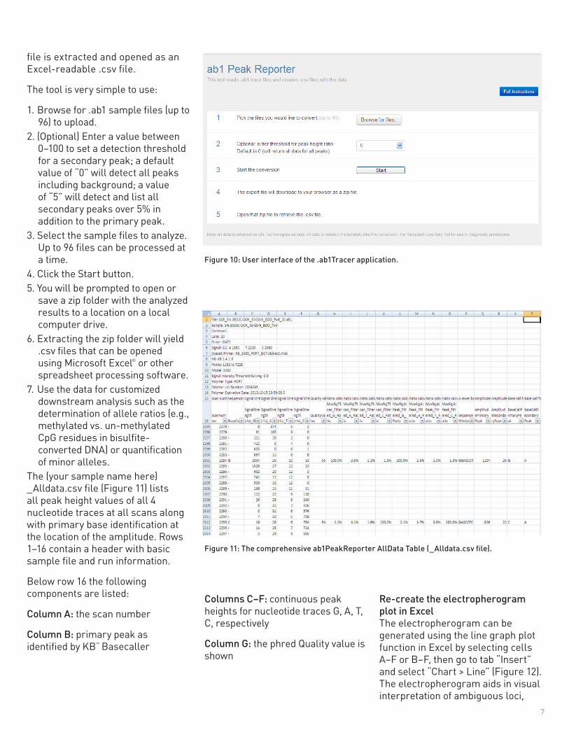
file is extracted and opened as an Excel-readable .csv file.

The tool is very simple to use:

1. Browse for .ab1 sample files (up to 96) to upload.

2. (Optional) Enter a value between 0–100 to set a detection threshold for a secondary peak; a default value of “0” will detect all peaks including background; a value of “5” will detect and list all secondary peaks over 5% in addition to the primary peak.

3. Select the sample files to analyze. Up to 96 files can be processed at a time.

4. Click the Start button.5. You will be prompted to open or

save a zip folder with the analyzed results to a location on a local computer drive.

6. Extracting the zip folder will yield .csv files that can be opened using Microsoft Excel® or other spreadsheet processing software.

7. Use the data for customized downstream analysis such as the determination of allele ratios (e.g., methylated vs. un-methylated CpG residues in bisulfite-converted DNA) or quantification of minor alleles.

The (your sample name here) _Alldata.csv file (Figure 11) lists all peak height values of all 4 nucleotide traces at all scans along with primary base identification at the location of the amplitude. Rows 1–16 contain a header with basic sample file and run information.

Below row 16 the following components are listed:

Column A: the scan number

Column B: primary peak as identified by KB™ Basecaller

Figure 10: User interface of the .ab1Tracer application.

Figure 11: The comprehensive ab1PeakReporter AllData Table (_Alldata.csv file).

Columns C–F: continuous peak heights for nucleotide traces G, A, T, C, respectively

Column G: the phred Quality value is shown

Re-create the electropherogram plot in ExcelThe electropherogram can be generated using the line graph plot function in Excel by selecting cells A–F or B–F, then go to tab “Insert” and select “Chart > Line” (Figure 12). The electropherogram aids in visual interpretation of ambiguous loci,

8

assisting in distinguishing genuine peaks from background noise or artifacts.

Applying filters aids in data explorationThe next step is to filter out the uncalled scans; this will enable customized display of data and is a great aid in exploring the data. To set filters click on row 16, go to tab “Data” and select “Filter” (Figure 13).

The Filter tool allows selective display of data by (un-)checking individual data points, sorting, and various ranges and rank formats in its “Number Filters” section.

Condensing the table to basecalled data onlyUsing the Filter tool, the table can be condensed to display only the basecalled data points. This feature is useful for transferring data into a database for subsequent archiving, and further exploratory or statistical analysis.

To condense the data table to basecalled data points only, 1) Click the Filter icon in column B, "BaseCall", 2) Uncheck the "–" box, 3) click the "OK" button (Figure 14).

Find loci of interest with “Sequence Window”To facilitate identification of an allele (nucleotide) of interest (e.g., a SNP) in the table, the “Sequence Window” can be used to display each base in the center of a string of 7 nucleotides (Figure 15). Use the 7-base string as input in Excel's "Search" and "Find" functions. Use a * character if the base in the middle of the string is unknown or N,Y,R, etc. This string of 7 nucleotides can also be used in Sequence Analysis or Sequence

Figure 12: Creating line plots of electropherograms. 1) Select cells A–F or B–F, 2) go to tab “Insert” and 3) select Line in the Chart section.

Figure 13: Applying Filters to the data. 1) Click on row 16, 2) go to tab “Data” and 3) select Filter.

1

23

1

23

9

Scanner software to readily find a peak of interest.

Ratio of maximal signals in a 7-scan window In columns I–L (Figure 15 )the peak height ratios in a 7-scan window of the maximal signal between the primary (i.e., basecalled) peak and the maximal signal of either G, A, T, C respectively is shown. What exactly are these numbers?

The peak height ratio is calculated as the maximum of heights measured at the scan of the amplitude and the 3 scans upstream and downstream (hence 7-scan) of that particular location.

Figure 16 shows an example of the MaxSig7Scan Ratio calculation: at scan location 799 a peak was called “N”; the highest peak was an “A” trace with 555 RFU, followed by a “T” trace with 438 RFU and C (14 RFU) and G (12 RFU) in a 7-scan window (highlighted in yellow) which is centered at the peak location and extends for 3 more scans on either side (3+1+3 = 7 scans). The ratio is calculated by dividing the peak height of the “primary” (i.e., highest) peak by the basecalled or highest peak height of either peak trace (G in column I, A in column J, T in column K, and T in column L) in the 7-scan window. One caveat: in traces with sub-optimal spacing or mobility overlap between adjacent bases it is possible that the trailing or leading slope of a legitimate adjacent peak is considered in this calculation which may produce an artificially higher ratio.

Ratio of signal in a 1-scan window at the basecall location In columns M–P the peak height ratios in a 1-scan window of the maximal signal between the primary (i.e., basecalled) peak and the signal of either G, A, T, C, respectively, is shown (Figure 17).

Figure 14: Condensing the data table to basecalled data points only.

Figure 15: The SequenceWindow lists 7-nucleotide strings, and can be used to facilitate finding a base of interest.

Figure 16: Ratios of maximal signal in a 7-scan window.

1

2

3

ACCTGTA

10

This ratio measurement is taken in a narrow window of one scan only. It may miss the amplitude of a peak under peak if it is outside this window. Therefore, both ratio measurements (7-scan and 1-scan) should be considered and possibly be combined (averaged), if necessary or warranted.

Data from the KB™ Basecaller (v1.4.1 and higher)Columns Q, R, S, T are populated with the amplitude and sequence output data from the KB™ Basecaller (Figure 18). Note that the amplitudes of the primary and secondary peak may differ from the original signal strength (RFU) shown in columns C–F. This is due to the mobility and other noise correction of the trace data during the basecalling process.

Column G lists the Quality value (phd or phred score) of the basecall (Figure 19).

Figure 17: The MaxSigAtPeak peak height ratio is determined by dividing the peak height of the primary peak (highest peak) by peak heights of either peak trace at the location (scan number) of the basecall.

Figure 18: Amplitudes and basecalls of primary and secondary peak as determined by KB™ Basecaller.

Figure 19: The Quality values indicate the probability of an incorrect basecall of primary peak.

Quality ValuesThe QV is a per-base estimate of the KB™ Basecaller accuracy. The QVs are calibrated on a scale corresponding to: QV = –10log10(Pe)where Pe is the probability of error.The KB™ Basecaller generates QVs from 1 to 99.Quality Value Probability the basecall is incorrect10 10%20 1%30 0.1%40 0.01%50 0.001%• Typical high-quality pure bases have QVs between 20–50• Typical high-quality mixed bases have QVs between 10–20

11

Measuring allele proportions by peak height ratiosTo demonstrate the utility of the tool we have prepared genomic DNA mixtures of normal and mutant TP53 gene (exon 11) at various proportions and determined the peak height ratios between minor and major allele using the ab1PeakReporter tool. Figure 20 shows that in this particular allele situation the peak height ratios obtained from both channels (1-scan window or 7-scan window) correlated quite well up to 15%. A 5% level of mutant allele was clearly distinguishable from 0% (normal control; Figure 21).

Figure 20: Peak height ratios.

Figure 21: Sequencing electropherograms of DNA mixtures prepared at various ratios of wt and mutant allele “697” in exon 11 of the human p53 gene as viewed in Sequence Scanner software. Note that the mutant allele was “called” as “S” at the 25% and 50% level but not below these ratios using the KB™ Basecaller.

0%

10%

5%

25%

2.5%

15%

7.5%

50%

12

ConclusionsThis application note shows tools and methods for extracting and using peak height data from fluorescent Sanger sequencing traces for determination of allele ratios or allele quantification. Table 1 summarizes the features of the two software applications presented.

QSVanalyzer ab1PeakReporter

Number of alleles Limited to predefined positions All bases in trace file

Number of .ab1 files that can be analyzed Multiple (maximum # not specified) QSV analysis requires presence of homozygous controls for either variant

96 (maximum upload per processing)

Table of peak height data of primary and secondary peaks

Yes (see Figure 6, columns B and C) Yes (requires that .ab1 file is analyzed with KB™ Basecaller v1.4)

Compatible data files .ab1, .scf .ab1

Peak traces displayed Yes, in comprehensive HTML report and in separate window as .png file

No, but can be created as a line graph in Excel using .csv file with complete data points

Output reports Folder with trace data, comprehensive QSV report in HTML and table (.xls) with raw and normalized peak heights and ratios

Zip folder with .csv file that opens in Microsoft Excel®

Suitable for quantitative assessment of SNPs, paralogous variant analysis and copy number variants

Yes (see Carr et al. 2009 for details) Delivers peak height data and peak height ratios for customized downstream analysis

Suitable for methylation analysis (sequencing of bisulfite-converted DNA)?

Can potentially provide allele ratios CpG to TpG (UpG). Delivers normalized peak height data for customized downstream analysis

Delivers peak height data for customized downstream analysis

Suitable for minor allele quantification (somatic or emerging mutations)?

Possible when used with appropriate calibrator controls, replicates and customized data analysis (polynomial regression), see Figure 7

Delivers peak height data for customized downstream analysis

Table 1: Summary of features available in the QSVanalyser application and the ab1PeakReporter tool.

References[1] Carr IM*, Robinson JI, Dimitriou R et al. (2009) Bioinformatics, 25 (24):3244–3250. http://bioinformatics.oxfordjournals.org/content/25/24/3244.long

[2] White paper: Applied Biosystems Genetic Analysis Data File Format http://www6.appliedbiosystems.com/support/software_community/ABIF_File_Format.pdf

Find out more at lifetechnologies.comFor Research Use Only. Not for use in diagnostic procedures. ©2013 Life Technologies Corporation. All rights reserved. The trademarks mentioned herein are the property of Life Technologies Corporation and/or its affiliate(s) or their respective owners. Excel is a registered trademark of Microsoft Corporation. CO07793 1113