detection and modeling of long memory in biases of … · detection and modeling of long memory in...
TRANSCRIPT

Detection and modeling of long memory in
biases of daily forecasts of air pressure
Yulia Gel, Bovas Abraham
Department of Statistics and Actuarial Science, University of Waterloo
1

OUTLINE
1. PROBLEM STATEMENT AND DATA DESCRIPTION.
2. MODEL CANDIDATES: DECAYING AVERAGING,
HOLT-WINTERS, ARMA, ARFIMA
3. TIME SERIES PROPERTIES OF BIASES
4. MODELS PREDICTIVE POWER
5. CONCLUSION
2

PROBLEM STATEMENT AND DATA DESCRIPTION
BIAS = FCST − ”OBS”,
where ”OBS” is a REANALY SIS.
GOAL is to predict future biases, ˆBIAS, from historical data. Then
FCSTcalibrated = FCSTOPR − ˆBIAS.
APPLICATION TO NCEP Operational Ensemble
DATA: NCEP T00Z 10 Ensemble Forecast of 500 MB HEIGHT, lead
time 12, 24, . . . , 384 hours (from 1 to 16 days ahead), 2001-2004.
LOCATIONS: 9 points worldwide
3

Figure 1: Data from 9 locations are analyzed.
−150 −100 −50 0 50 100
−100
−50
050
100
4

MODEL CANDIDATES
• Decaying Averaging (DA) is the NCEP Adaptive (Kalman Filter
Type) Bias-Correction Algorithm – variation of the Single
Exponential Smoothing (SES)
ˆBIAS = (1−ω)×prior t.m.e.+ω×the most recent BIAS,
– for each lead time separately;
– t.m.e.=time mean error which is calculated using historical
biases within the sliding window of 30 most recent days;
– ω = 2% is selected subjectively (for some not included
locations ω is 5% or 10%)
5

• Holt-Winters (HW) Smoothing – extension of DA and SES
which
– takes into account linear trends and additive or multiplicative
seasonality (if any is detected).
– is known to provide poor long term predictions
• ARMA(p, q) – Autoregressive Moving Average Model
a(B)yt = b(B)vt,
– a(·) and b(·) are polynomials of degree p and q,
vt ∼ WN(0, 1).
– the autocorrelation function (acf) decays exponentially, i.e. a
short memory process.
6

• ARFIMA(p, d, q) – Fractionally Integrated Autoregressive
Moving Average (long memory) model
a(B)(1−B)dyt = b(B)vt, d ∈ (−0.5, 0.5).
– a(·) and b(·) are polynomials of degree p and q,
vt ∼ WN(0, 1).
– the autocorrelation function (acf) decays geometrically, i.e. a long
memory process.
7

• Two Stage Procedure – Sliding Window Demeaning + Linear
Models:
– estimate parameters of a linear time series model, e.g. an ARMA
or ARFIMA model, whose coefficients are obtained using the
most recent available biases (sliding large window parameter
estimation);
– removes the mean calculated on the most recent available raw
biases (sliding short window demeaning).
8
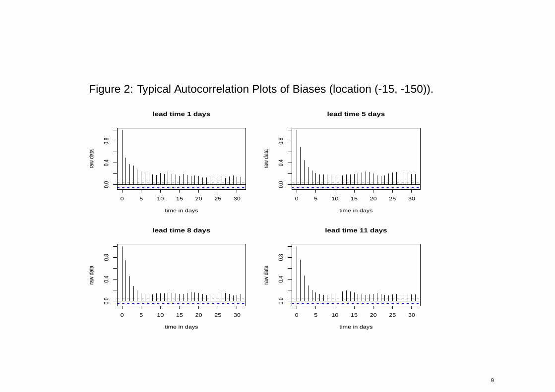
Figure 2: Typical Autocorrelation Plots of Biases (location (-15, -150)).
0 5 10 15 20 25 30
0.0
0.4
0.8
time in days
raw
data
lead time 1 days
0 5 10 15 20 25 30
0.0
0.4
0.8
time in days
raw
data
lead time 5 days
0 5 10 15 20 25 30
0.0
0.4
0.8
time in days
raw
data
lead time 8 days
0 5 10 15 20 25 30
0.0
0.4
0.8
time in days
raw
data
lead time 11 days
9
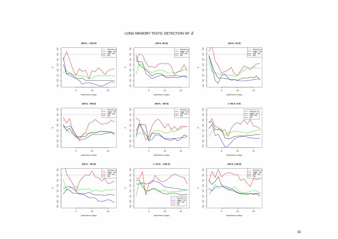
LONG MEMORY TESTS: DETECTION OF d
(60.0, −120.0)
lead time in days
d
5 10 15
−0.1
0.0
0.1
0.2
0.3
0.4
0.5
0.6
Period−mAggr. VarDiff. VarML
(35.0, 60.0)
lead time in days
d
5 10 15
−0.1
0.0
0.1
0.2
0.3
0.4
0.5
0.6
Period−mAggr. VarDiff. VarML
(40.0, 15.0)
lead time in days
d
5 10 15
−0.1
0.0
0.1
0.2
0.3
0.4
0.5
0.6
Period−mAggr. VarDiff. VarML
(40.0, −95.0)
lead time in days
d
5 10 15
−0.1
0.0
0.1
0.2
0.3
0.4
0.5
0.6
Period−mAggr. VarDiff. VarML
(40.0, −50.0)
lead time in days
d
5 10 15
−0.1
0.0
0.1
0.2
0.3
0.4
0.5
0.6
Period−mAggr. VarDiff. VarML
(−45.0, 0.0)
lead time in days
d
5 10 15
−0.1
0.0
0.1
0.2
0.3
0.4
0.5
0.6
Period−mAggr. VarDiff. VarML
(25.0, −90.0)
lead time in days
d
5 10 15
−0.1
0.0
0.1
0.2
0.3
0.4
0.5
0.6
Period−mAggr. VarDiff. VarML
(−15.0, −150.0)
lead time in days
d
5 10 15
−0.1
0.0
0.1
0.2
0.3
0.4
0.5
0.6
Period−mAggr. VarDiff. VarML
(40.0, 118.0)
lead time in days
d
5 10 15
−0.1
0.0
0.1
0.2
0.3
0.4
0.5
0.6
Period−mAggr. VarDiff. VarML
10

Figure 3: Predictive Power of the Two Stage Procedure: Sliding Window Demeaning + Linear Time
Series Models. The Plots of the Raw and Corrected Root Mean Square Errors (RMSE) (left) and
their ratios 1 − CorrectedRMSERawRMSE
(right) (positive values imply improvement, negative ratios imply
deterioration). DA is the Decaying Averaging method.
0 2 4 6 8 10 12 14 16 180
5
10
15
20
25(−15, −150)
Lead Time (in days)
Roo
t Mea
n S
quar
e E
rror
(R
MS
E)
Raw BiasDAARMA(1,1)
win=500ARMA(5,5)
win=1000ARFIMA(1,d,1)
AR(70)
0 2 4 6 8 10 12 14 16 18−20
−15
−10
−5
0
5
10
15
20
25
30(−15, −150)
Lead Time (in days)
Impr
ovem
ent (
posi
tive)
or
dete
riora
tion
(neg
ativ
e) o
f RM
SE
(in
%)
DAARMA(1,1)
win=500ARMA(5,5)
win=1000ARFIMA(1,d,1)
AR(70)
11
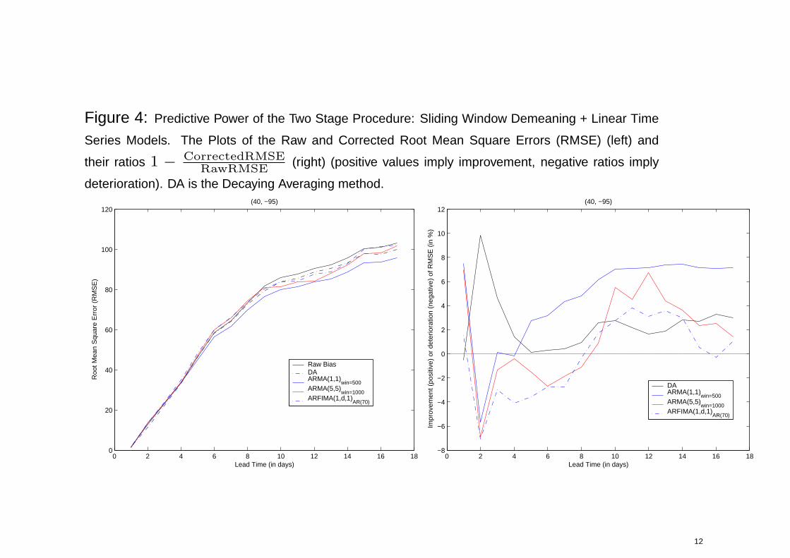
Figure 4: Predictive Power of the Two Stage Procedure: Sliding Window Demeaning + Linear Time
Series Models. The Plots of the Raw and Corrected Root Mean Square Errors (RMSE) (left) and
their ratios 1 − CorrectedRMSERawRMSE
(right) (positive values imply improvement, negative ratios imply
deterioration). DA is the Decaying Averaging method.
0 2 4 6 8 10 12 14 16 180
20
40
60
80
100
120(40, −95)
Lead Time (in days)
Roo
t Mea
n S
quar
e E
rror
(R
MS
E)
Raw BiasDAARMA(1,1)
win=500ARMA(5,5)
win=1000ARFIMA(1,d,1)
AR(70)
0 2 4 6 8 10 12 14 16 18−8
−6
−4
−2
0
2
4
6
8
10
12(40, −95)
Lead Time (in days)
Impr
ovem
ent (
posi
tive)
or
dete
riora
tion
(neg
ativ
e) o
f RM
SE
(in
%)
DAARMA(1,1)
win=500ARMA(5,5)
win=1000ARFIMA(1,d,1)
AR(70)
12

Figure 5: Predictive Power of the Two Stage Procedure: Sliding Window Demeaning + Linear Time
Series Models. The Plots of the Raw and Corrected Root Mean Square Errors (RMSE) (left) and
their ratios 1 − CorrectedRMSERawRMSE
(right) (positive values imply improvement, negative ratios imply
deterioration). DA is the Decaying Averaging method.
0 2 4 6 8 10 12 14 16 180
20
40
60
80
100
120(60, −120)
Lead Time (in days)
Roo
t Mea
n S
quar
e E
rror
(R
MS
E)
Raw BiasDAARMA(1,1)
win=500ARMA(5,5)
win=1000ARFIMA(1,d,1)
AR(70)
0 2 4 6 8 10 12 14 16 18−6
−4
−2
0
2
4
6
8
10
12(60, −120)
Lead Time (in days)
Impr
ovem
ent (
posi
tive)
or
dete
riora
tion
(neg
ativ
e) o
f RM
SE
(in
%)
DAARMA(1,1)
win=500ARMA(5,5)
win=1000ARFIMA(1,d,1)
AR(70)
13

Figure 6: Predictive Power of the Two Stage Procedure: Sliding Window Demeaning + Linear Time
Series Models. The Plots of the Raw and Corrected Root Mean Square Errors (RMSE) (left) and
their ratios 1 − CorrectedRMSERawRMSE
(right) (positive values imply improvement, negative ratios imply
deterioration). DA is the Decaying Averaging method.
0 2 4 6 8 10 12 14 16 180
5
10
15
20
25
30
35
40
45
50(25, −90)
Lead Time (in days)
Roo
t Mea
n S
quar
e E
rror
(R
MS
E)
Raw BiasDAARMA(1,1)
win=500ARMA(5,5)
win=1000ARFIMA(1,d,1)
AR(70)
0 2 4 6 8 10 12 14 16 18−10
−5
0
5
10
15
20
25
30
35(25, −90)
Lead Time (in days)
Impr
ovem
ent (
posi
tive)
or
dete
riora
tion
(neg
ativ
e) o
f RM
SE
(in
%)
DAARMA(1,1)
win=500ARMA(5,5)
win=1000ARFIMA(1,d,1)
AR(70)
14

Figure 7: Predictive Power of the Two Stage Procedure: Sliding Window Demeaning + Linear Time
Series Models. The Plots of the Raw and Corrected Root Mean Square Errors (RMSE) (left) and
their ratios 1 − CorrectedRMSERawRMSE
(right) (positive values imply improvement, negative ratios imply
deterioration).DA is the Decaying Averaging method.
0 2 4 6 8 10 12 14 16 180
10
20
30
40
50
60
70
80
90(40, 118)
Lead Time (in days)
Roo
t Mea
n S
quar
e E
rror
(R
MS
E)
Raw BiasDAARMA(1,1)
win=500ARMA(5,5)
win=1000ARFIMA(1,d,1)
AR(70)
0 2 4 6 8 10 12 14 16 18−6
−4
−2
0
2
4
6
8(40, 118)
Lead Time (in days)
Impr
ovem
ent (
posi
tive)
or
dete
riora
tion
(neg
ativ
e) o
f RM
SE
(in
%)
DAARMA(1,1)
win=500ARMA(5,5)
win=1000ARFIMA(1,d,1)
AR(70)
15

Figure 8: Predictive Power of the Two Stage Procedure: Sliding Window Demeaning + Linear Time
Series Models. The Plots of the Raw and Corrected Root Mean Square Errors (RMSE) (left) and
their ratios 1 − CorrectedRMSERawRMSE
(right) (positive values imply improvement, negative ratios imply
deterioration). DA is the Decaying Averaging method.
0 2 4 6 8 10 12 14 16 180
10
20
30
40
50
60(35, 60)
Lead Time (in days)
Roo
t Mea
n S
quar
e E
rror
(R
MS
E)
Raw BiasDAARMA(1,1)
win=500ARMA(5,5)
win=1000ARFIMA(1,d,1)
AR(70)
0 2 4 6 8 10 12 14 16 18−10
−5
0
5
10
15(35, 60)
Lead Time (in days)
Impr
ovem
ent (
posi
tive)
or
dete
riora
tion
(neg
ativ
e) o
f RM
SE
(in
%)
DAARMA(1,1)
win=500ARMA(5,5)
win=1000ARFIMA(1,d,1)
AR(70)
16
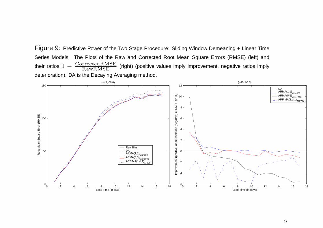
Figure 9: Predictive Power of the Two Stage Procedure: Sliding Window Demeaning + Linear Time
Series Models. The Plots of the Raw and Corrected Root Mean Square Errors (RMSE) (left) and
their ratios 1 − CorrectedRMSERawRMSE
(right) (positive values imply improvement, negative ratios imply
deterioration). DA is the Decaying Averaging method.
0 2 4 6 8 10 12 14 16 180
50
100
150(−45, 00.0)
Lead Time (in days)
Roo
t Mea
n S
quar
e E
rror
(R
MS
E)
Raw BiasDAARMA(1,1)
win=500ARMA(5,5)
win=1000ARFIMA(1,d,1)
AR(70)
0 2 4 6 8 10 12 14 16 18−6
−4
−2
0
2
4
6
8
10
12(−45, 00.0)
Lead Time (in days)
Impr
ovem
ent (
posi
tive)
or
dete
riora
tion
(neg
ativ
e) o
f RM
SE
(in
%)
DAARMA(1,1)
win=500ARMA(5,5)
win=1000ARFIMA(1,d,1)
AR(70)
17

Figure 10: Predictive Power of the Two Stage Procedure: Sliding Window Demeaning + Linear
Time Series Models. The Plots of the Raw and Corrected Root Mean Square Errors (RMSE) (left) and
their ratios 1 − CorrectedRMSERawRMSE
(right) (positive values imply improvement, negative ratios imply
deterioration). DA is the Decaying Averaging method.
0 2 4 6 8 10 12 14 16 180
20
40
60
80
100
120(40, 15)
Lead Time (in days)
Roo
t Mea
n S
quar
e E
rror
(R
MS
E)
Raw BiasDAARMA(1,1)
win=500ARMA(5,5)
win=1000ARFIMA(1,d,1)
AR(70)
0 2 4 6 8 10 12 14 16 18−6
−4
−2
0
2
4
6
8
10
12
14(40, 15)
Lead Time (in days)
Impr
ovem
ent (
posi
tive)
or
dete
riora
tion
(neg
ativ
e) o
f RM
SE
(in
%)
DAARMA(1,1)
win=500ARMA(5,5)
win=1000ARFIMA(1,d,1)
AR(70)
18

Figure 11: Predictive Power of the Two Stage Procedure: Sliding Window Demeaning + Linear
Time Series Models. The Plots of the Raw and Corrected Root Mean Square Errors (RMSE) (left) and
their ratios 1 − CorrectedRMSERawRMSE
(right) (positive values imply improvement, negative ratios imply
deterioration). DA is the Decaying Averaging method.
0 2 4 6 8 10 12 14 16 180
20
40
60
80
100
120
140(40, −50)
Lead Time (in days)
Roo
t Mea
n S
quar
e E
rror
(R
MS
E)
Raw BiasDAARMA(1,1)
win=500ARMA(5,5)
win=1000ARFIMA(1,d,1)
AR(70)
0 2 4 6 8 10 12 14 16 18−8
−6
−4
−2
0
2
4(40, −50)
Lead Time (in days)
Impr
ovem
ent (
posi
tive)
or
dete
riora
tion
(neg
ativ
e) o
f RM
SE
(in
%)
DAARMA(1,1)
win=500ARMA(5,5)
win=1000ARFIMA(1,d,1)
AR(70)
19
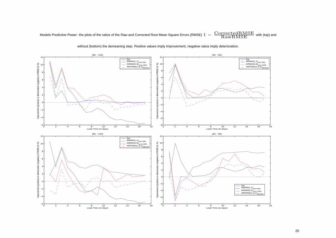
Models Predictive Power: the plots of the ratios of the Raw and Corrected Root Mean Square Errors (RMSE) 1 − CorrectedRMSERawRMSE with (top) and
without (bottom) the demeaning step. Positive values imply improvement, negative ratios imply deterioration.
0 2 4 6 8 10 12 14 16 18−6
−4
−2
0
2
4
6
8
10
12(60, −120)
Lead Time (in days)
Impr
ovem
ent (
posit
ive) o
r det
erio
ratio
n (n
egat
ive) o
f RM
SE (i
n %
)
DAARMA(1,1)
win=500ARMA(5,5)
win=1000ARFIMA(1,d,1)
AR(70)
0 2 4 6 8 10 12 14 16 18−8
−6
−4
−2
0
2
4
6
8
10
12(40, −95)
Lead Time (in days)
Impr
ovem
ent (
posit
ive) o
r det
erio
ratio
n (n
egat
ive) o
f RM
SE (i
n %
)
DAARMA(1,1)
win=500ARMA(5,5)
win=1000ARFIMA(1,d,1)
AR(70)
20

Models Predictive Power: the plots of the ratios of the Raw and Corrected Root Mean Square Errors (RMSE) 1 − CorrectedRMSERawRMSE with (bottom) and
without (top) the demeaning step. Positive values imply improvement, negative ratios imply deterioration.
0 2 4 6 8 10 12 14 16 18−20
−15
−10
−5
0
5
10
15
20
25
30(−15, −150)
Lead Time (in days)
Impr
ovem
ent (
posi
tive)
or d
eter
iora
tion
(neg
ativ
e) o
f RM
SE (i
n %
)
DAARMA(1,1)
win=500ARMA(5,5)
win=1000ARFIMA(1,d,1)
AR(70)
0 2 4 6 8 10 12 14 16 18−10
−5
0
5
10
15
20
25
30
35(25, −90)
Lead Time (in days)
Impr
ovem
ent (
posi
tive)
or d
eter
iora
tion
(neg
ativ
e) o
f RM
SE (i
n %
)
DAARMA(1,1)
win=500ARMA(5,5)
win=1000ARFIMA(1,d,1)
AR(70)
21

Models Predictive Power: the plots of the ratios of the Raw and Corrected Root Mean Square Errors (RMSE) 1 − CorrectedRMSERawRMSE with (bottom) and
without (top) the demeaning step. Positive values imply improvement, negative ratios imply deterioration.
0 2 4 6 8 10 12 14 16 18−6
−4
−2
0
2
4
6
8(40, 118)
Lead Time (in days)
Impr
ovem
ent (
posit
ive) o
r det
erio
ratio
n (n
egat
ive) o
f RM
SE (i
n %
)
DAARMA(1,1)
win=500ARMA(5,5)
win=1000ARFIMA(1,d,1)
AR(70)
0 2 4 6 8 10 12 14 16 18−10
−5
0
5
10
15(35, 60)
Lead Time (in days)
Impr
ovem
ent (
posi
tive)
or d
eter
iora
tion
(neg
ativ
e) o
f RM
SE (i
n %
)
DAARMA(1,1)
win=500ARMA(5,5)
win=1000ARFIMA(1,d,1)
AR(70)
22

Models Predictive Power: the plots of the ratios of the Raw and Corrected Root Mean Square Errors (RMSE) 1 − CorrectedRMSERawRMSE with (bottom) and
without (top) the demeaning step. Positive values imply improvement, negative ratios imply deterioration.
0 2 4 6 8 10 12 14 16 18−6
−4
−2
0
2
4
6
8
10
12(−45, 00.0)
Lead Time (in days)
Impr
ovem
ent (
posit
ive) o
r det
erio
ratio
n (n
egat
ive) o
f RM
SE (i
n %
)
DAARMA(1,1)
win=500ARMA(5,5)
win=1000ARFIMA(1,d,1)
AR(70)
0 2 4 6 8 10 12 14 16 18−6
−4
−2
0
2
4
6
8
10
12
14(40, 15)
Lead Time (in days)
Impr
ovem
ent (
posit
ive) o
r det
erio
ratio
n (n
egat
ive) o
f RM
SE (i
n %
)
DAARMA(1,1)
win=500ARMA(5,5)
win=1000ARFIMA(1,d,1)
AR(70)
0 2 4 6 8 10 12 14 16 18−6
−4
−2
0
2
4
6
8
10
12(−45, 00.0)
Lead Time (in days)
Impr
ovem
ent (
posit
ive) o
r det
erio
ratio
n (n
egat
ive) o
f RM
SE (i
n %
)
DAARMA(1,1)
win=500ARMA(5,5)
win=1000ARFIMA(1,d,1)
AR(70)
0 2 4 6 8 10 12 14 16 18−6
−4
−2
0
2
4
6
8
10
12
14(40, 15)
Lead Time (in days)
Impr
ovem
ent (
posit
ive) o
r det
erio
ratio
n (n
egat
ive) o
f RM
SE (i
n %
)
DAARMA(1,1)
win=500ARMA(5,5)
win=1000ARFIMA(1,d,1)
AR(70)
23
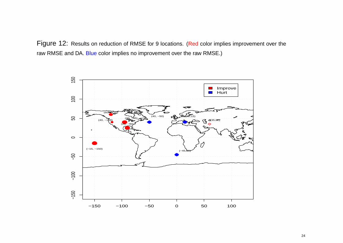
Figure 12: Results on reduction of RMSE for 9 locations. (Red color implies improvement over the
raw RMSE and DA. Blue color implies no improvement over the raw RMSE.)
−150 −100 −50 0 50 100
−150
−100
−50
050
100
150
ImproveHurt
(35,60)
(25, −90)
(40,15)
(−45,00)
(40, −50)(40, −95)
(60, −120)
(40, −118)
(−15, −150)
24

CONCLUSION• Biases at all 9 location and all lead times exhibit a long memory pattern of
various degrees.
• There exists a remarkable change (drop) in the pattern of the estimated d
around lead time 5 days for most locations.
• DA method performs well up to around lead time 5 days and then significantly
degrades, e.g. even deteriorates RMSE instead of improving it. (Is there any
connection between the change of d and degrading of DA around day 5?)
25

• ARMA, ARFIMA models without a smoothed demeaning show similar
performance for short lead time and are generally close to DA results. For
longer lead times they provide no improvement and no harm (with some
minor deviations from location to location).
• In contrast, the two stage procedure (demeaning + ARMA) provides a
noticeable improvement for high lead times for locations in the North America.
26