Sequential Analysis, 26: 225–249, 2007Copyright © Taylor & Francis Group, LLCISSN: 0747-4946 print/1532-4176 onlineDOI: 10.1080/07474940701404765

Detection and Diagnosis of Unknown AbruptChanges Using CUSUMMulti-Chart Schemes

Dong HanDepartment of Mathematics, Shanghai Jiao Tong University, Shanghai, China

Fugee TsungDepartment of Industrial Engineering and Logistics Management,

Hong Kong University of Science and Technology, Kowloon, Hong Kong

Abstract: A cumulative sum (CUSUM) multi-chart scheme that consists of multipleCUSUM control charts is studied for detecting and diagnosing an unknown abrupt changein a stochastic system on the basis of sequential observations. We prove that the CUSUMmulti-chart not only has a high diagnostic capability but also possesses a better detectionperformance than individual CUSUM charts when the in-control average run length is large.We also present an optimal design of the CUSUM multi-chart and two illustrative examplesinvolving the normal and exponential distributions. Moreover, numerical comparisons ofthe average run lengths are made via Monte Carlo simulation among the CUSUM,generalized likelihood ratio, exponentially weighted moving average (EWMA), multi-chart,and CUSUM multi-chart. The numerical results indicate that the CUSUM multi-chart hasthe best performance on the whole among the five schemes in detecting the unknownmean shift.

Keywords: Asymptotic optimality; Kullback–Leibler information distances; Online detectionand diagnosis; Sequential analysis.

Subject Classifications: 62L10; 62N10.

1. INTRODUCTION

The problem of quick detection and diagnosis of abrupt changes in a stochasticsystem has many important applications, including industrial quality control,

Received December 18, 2005, Revised March 13, 2006, Accepted April 9, 2006Recommended by W. SchmidAddress correspondence to Fugee Tsung, Department of Industrial Engineering

and Logistics Management, Hong Kong University of Science and Technology, Kowloon,Hong Kong; E-mail: season@ust.hk

226 Han and Tsung

automated fault detection in controlled dynamical systems, segmentation of signals,and so on. To deal with the problem, various control charts, such as Shewhartcharts, cumulative sum (CUSUM) charts, exponentially weighted moving average(EWMA) charts, cumulative score (Cuscore) charts, etc. have been proposed.Many studies on these control charts have been conducted by Crowder (1987,1989), Lucas and Saccucci (1990), Montgomery and Mastrangelo (1991), Baxley(1995), Mastrangelo and Montgomery (1995), Lai (1995), Reynolds (1996a,b), Boxand Luceño (1997), Ramírez (1998), Hawkins and Olwell (1998), Luceño (1999),Mastrangelo and Brown (2000), Jiang et al. (2000), Jones et al. (2001), and Shu et al.(2002).

Moustakides (1986) and Ritov (1990) proved that the performance in detectingthe mean shift of the one-sided CUSUM control chart with the reference value, �,which is related to the mean shift magnitude of particular interest, is optimal interms of the average run length (ARL) if the real mean shift is �. In reality, we rarelyknow the exact shift value of a process before detecting the mean shift. That is tosay, the performance of the CUSUM chart in detecting the mean shift depends onthe given reference value, which is the magnitude of the mean shift to be detectedquickly. For the same reason, the detecting performance of many other controlcharts, such as the EWMA, the optimal EWMA, and Cuscore, is closely relatedto the given reference value or the reference pattern. Moreover, it is challenging todiagnose the possible size of the mean shift quickly by using a single control chart.

There are several schemes that do not depend on a specific shift size �. Forexample, using the generalized likelihood ratio (GLR) statistic, Siegmund andVenkatraman (1995) presented a CUSUM-like control chart, called the GLR chart,that does not depend on the value of �. Their simulation results show that the GLRchart is better than the CUSUM control chart in detecting a mean shift that is largeror smaller than � and is only slightly inferior in detecting a mean shift of size �. Also,by taking the maximum weighting parameter in the EWMA control chart, Han andTsung (2004) proposed a generalized EWMA (GEWMA) control chart that doesnot depend on the reference value and proved that the GEWMA control chart isbetter than the optimal EWMA in detecting a mean shift of any size when the in-control ARL is large. However, these methods usually require complex computingand thus have not been regularly applied to real online problems in practice.

To solve the problem of detecting the unknown magnitude of the change,various detection schemes have been proposed and studied. The pioneering workon this issue was done by Lorden (1971) and Lorden and Eisenberger (1973)on charting a set of CUSUM statistics. Dragalin (1993, 1997) investigated thedesign and analysis of a combination of two CUSUM charts. Sparks (2000) furtherexplored this idea and studied a combination of three CUSUM charts in particularvia simulation. On the other hand, Willsky and Jones (1976) introduced the window-limited GLR scheme, which was theoretically investigated by Lai (1995, 1998) andby Lai and Shan (1999). Although the window-limited GLR scheme and the GLRcontrol chart have good performance in detecting the unknown magnitude of thechanges, their computational complexity and lack of a capability in diagnosing thepossible magnitude of the changes restrict their application in real online problems.To make the GLR scheme practicable, Nikiforov (2000) proposed a suboptimalrecursive approach that is based on a collection of L parallel recursive �2-CUSUMcharts and established a direct relation between the efficiency of the detection

Detection and Diagnosis of Unknown Abrupt Changes 227

scheme and its computational complexity. Motivated by Nikiforov’s recursiveapproach, we further extend the study of the CUSUM multi-chart.

The objective of this paper is to demonstrate that the CUSUM multi-chartcan meet to a considerable extent the following three goals in detecting anddiagnosing the unknown abrupt change in a stochastic system: (1) signal an alarmas quickly as possible when having an abrupt change, (2) accurately indicate thepossible type/amount/size/etc. of the change, and (3) easily handle computationalcomplexity.

The remainder of this paper is organized as follows. In Section 2, the CUSUMmulti-chart and a charting performance index (CPI) to evaluate the detection powerof a control chart over a whole region of possible abrupt changes are introduced.The asymptotic ARLs, optimal design, and diagnostic capability of the CUSUMmulti-chart are presented in Section 3. Two illustrative examples and simulationcomparisons are demonstrated in Section 4. Conclusions and problems for furtherstudy are discussed in Section 5, with the proofs of two lemmas and two theoremsgiven in the appendix.

2. THE CUSUM MULTI-CHART SCHEME

Let Xi� i = 1� 2� � � � be the ith independent observation on a process with a knowncommon probability distribution, f�0 . Suppose that at some time period, �, whichis usually called a change point, the probability distribution of Xi changes fromf�0 to f�, where f� �= f�0 if and only if � �= �0. In other words, from time period �onwards, Xi has the common distribution f�. Note that the parameter � may not bethe characteristic number of the distribution f�, for example, the mean, deviation,etc., which is often used just to distinguish the different distributions. In practice, thechange point and the postchange distributions are usually unknown, that is, � and �are two unknown parameters. However, we may assume that the possible unknownpostchange distributions �f�� belong to a closed domain D�, where D� = �f� �� ∈ D��D is a closed boundary set of the parameters, and the boundary D of D isknown.

The possible change domain and its boundary (including the size and form ofthe boundary) about the observation process may be determined by engineeringknowledge, practical experience, or statistical data if the possible unknownpostchange, �f��, is a dominated family of distributions with parameters �.For example, when f� is the normal density function and � = a� b�, where aand b denote the mean and standard deviation respectively, we can take theset D = �a� b� � a1 ≤ a ≤ a2� 0 < b1 ≤ b ≤ b2�, where a1� a2� b1, and b2 are knownnumbers, which means that we know the domain of the possible postchangedistributions, that is, the boundary D of the parameter set is known. Notethat the mean of the process with gamma distribution �� �� may keep with aconstant when the postchange occurs since the mean of the gamma distributionis �/�, where � = �� �� are the parameters of gamma distribution. If �f�� issubject to a family of multidistributions, for example, multinormal distributionsN�1� �2� �� �

21� �

22�, we can similarly choose a closed boundary set D of the

parameters � = �1� �2� �� �1� �2�� If the possible postchange distributions consist oftwo kinds of family distributions (normal and stable distributions), it is not clear

228 Han and Tsung

and easy for us to choose a closed boundary set satisfying conditions I and IIdefined in Section 3.

In this paper we mainly consider the case that the possible postchangedistributions belong to a set that consists of a dominated family of distributions �f��with the parameter �. Moreover, we assume that �0 � D and f� �= f�′ if and onlyif � �= �′, where f�, f�′ ∈ D�, and �� �′ ∈ D. In order to detect and diagnose theunknown abrupt changes, the CUSUM multi-chart, TMC , is defined as follows: fixedm ≥ 2

TMC = min1≤k≤m

�T�k� dk��

T�k� dk� = min{n � max

1≤j≤n

n∑i=j

logf�kXi�

f�0Xi�> dk

}�

where dk > 0� 1 ≤ k ≤ m� are control limits; �k ∈ D and f�k ∈ D�, 1 ≤ k ≤ m areprespecified known reference values and density functions, respectively; and f�0 is aknown common probability density of �Xi� before the change point.

Let E�·�, E�0·�, and E�k

·�� 1 ≤ k ≤ m denote the expectations correspondingto the unknown postchange density, f�; the known common probability density, f�0 ;and the known reference density functions, f�k� 1 ≤ k ≤ m, respectively. We oftenuse ARL�·� and ARL0·� to denote E�·� and E�0

·�, respectively.The unknown abrupt change, f�, will be detected and diagnosed according

to the following procedure. Take the control limits, dk� 1 ≤ k ≤ m, such thatE�0

T�k� dk�� = L for all 1 ≤ k ≤ m, where the number L is a positive constant. Ifthe CUSUM multi-chart test, TMC , sends out an alarm of having an abrupt change,the alarm certainly comes from one of the CUSUM charts, for example, T�l� dl�.That is, T�l� dl� is the first one to tell us that the change occurs. In this case,we may say that the unknown postchange probability density, f�, is near f�l sincethe CUSUM chart with the reference density function f�l has the best detectionperformance in terms of the ARL� if the real postchange is f�l . Here the chart hasthe best detection performance means that it has the smallest ARL� among them CUSUM charts with common ARL0, that is, E�l

T�l� dl�� < E�lT�k� dk�� for

k �= l, 1 ≤ k ≤ m.In order to evaluate the detection power of a control chart, T with E�0

T� = L,over a whole region of possible abrupt changes, we present the CPI in the following:

CPIT� = exp{−∫Dw��

E�T�−ARL∗�

ARL∗�

d�

}�

where ARL∗� is a reference ARL value of well-known procedure at the postchange

probability density, f�, and w�� is a positive weighting function with∫Dw��d� = 1

to emphasize various postchanges within the region D� based on prior knowledgeand experience with the process. Usually, we may take w�� such that w�′� >w�� when I�0� �

′� > I�0� �� if the “large” change is considered more importantthan the “small” change. Thus, we can compare the charts by the CPI to knowwhich performs better in detecting such a large change. If no prior information andpreference are provided, we may use a equal weight w�� = MD�−1 throughout theregion, where M·� is a measure of the region D.

Detection and Diagnosis of Unknown Abrupt Changes 229

Let I�� �0� denote the Kullback–Leibler information distance (number)defined by

I�� �0� = E�

[log

f�X�

f�0X�

]�

Taking

ARL∗� ∼

logLI�� �0�

� (2.1)

which is Lorden’s (1971) asymptotic lower bound, that is, as L →

infT�E0T�≥L

E�T� ∼logLI�� �0�

where

E�T� = supn≥1

ess supE��T − n+ 1�+ �X1� � � � � Xn−1�

and n is change time, we have 0 < CPIT� ≤ 1 for large L if E�T� ≥ E�T� forlarge L. Obviously, the higher the CPI the better detection performance for thechart. Compared with traditional evaluation methods using ARL at a single point,the proposed CPI can take the whole postchange region into consideration.

3. THE ASYMPTOTIC ARL AND THE DIAGNOSTIC CAPABILITYOF THE CUSUM MULTI-CHART

In this section, we first present the asymptotic ARL. We then introduce the optimaldesign and diagnostic capability of the CUSUM multi-chart for the unknownabrupt change, that is, the unknown postchange probability density function f�.

3.1. The Asymptotic ARL and the Optimal Design of the CUSUM Multi-Chart

In order to obtain the asymptotic ARL of the CUSUM multi-chart, we first dividethe region, D�, into several disjointed subsets by using the reference densityfunctions, f�k� 1 ≤ k ≤ m� according to the Kullback–Leibler information distance.

Let the prespecified reference density functions be f�k ∈ D� and �k ∈ D,1 ≤ k ≤ m. Let

Jk ={f� ∈ D� � I�� �k� ≤ min

j �=kI�� �j�

}

for 1 ≤ k ≤ m and

1 = J1� k = Jk − Jk ∩k−1⋃j=1

Jj

230 Han and Tsung

for 2 ≤ k ≤ m, where f�0 � D� is the known density function before the abruptchange. It can be seen that the sets k, k = 1� 2� � � � � m� are disjointed and

⋃mk=1 k =

D�. Since f� �= f�′ if and only if � �= �′, we have a disjointed division of the regionD, Dk, k = 1� 2� � � � � m� such that

⋃mk=1 Dk = D, �k ∈ Dk, and � ∈ Dk if and only if

f� ∈ k 1 ≤ k ≤ m�. Thus, the CPITMC� can be written as

CPITMC� = exp{−

m∑k=1

∫Dk

w��E�TMC�−ARL∗

�

ARL∗�

d�

}� (3.1)

To estimate the ARL of the CUSUM multi-chart scheme, we define a generalizedKullback–Leibler information distance (number), I�� �k� �0�, as

I�� �k� �0� = E�

[log

f�kX�

f�0X�

]= I�� �0�− I�� �k��

for 1 ≤ k ≤ m. Note that the number I�� �k� �0� may be negative. Obviously,I�k� �k� �0� = I�k� �0� or 0 if � = �k or �k = �0. Moreover, by the definitionof k, we have f� ∈ k − k (or � ∈ Dk − Dk) if and only if I�� �k� �0� >maxj �=k�I�� �j� �0�� since I�� �k� �0� = I�� �0�− I�� �k� can only occur on k.Thus, we can say that the unknown postchange probability density function, f�, isnear the prespecified reference density function, f�k (or � is near the prespecifiedreference value, �k) if and only if f� ∈ k (� ∈ Dk).

Here, we assume that the chosen reference density functions, f�k ∈ D�� 1 ≤k ≤ m� satisfy the following conditions:

I. 0 < I�0� �k� < I�0� �k+1� for 1 ≤ k ≤ m− 1.II. I�� �k� �0� > 0 if f� ∈ k or � ∈ Dk for 1 ≤ k ≤ m.III. For each f� ∈ k and f�k , 1 ≤ k ≤ m, there exists a positive number � such that

E�0exp�� � log�f�kX�/f�0X�� � �� < � E�exp�� � log�f�kX�/f�0X�� � �� < �

Moreover, the random variables log�f�kX�/f�0X��, 1 ≤ k ≤ m� are not degenerate.Condition I implies that the reference density function, f�k+1

, is farther fromf�0 than from f�k according to the meaning of the Kullback–Leibler informationdistance (number). The inequality I�� �k� �0� > 0, that is, I�� �0� > I�� �k�, impliesthat the information distance between f� and f�0 is greater than that between f� andf�k . Thus, condition II can hold if we take many f�k , 1 ≤ k ≤ m, such that I�� �0� >I�� �k� for all f� ∈ k (1 ≤ k ≤ m). Condition III is just Cramèr’s condition (seeShiryaev, 1995). This condition means that E�0

�log�f�kX�/f�0X���n� < andE��log�f�kX�/f�0X���n� < for n ≥ 1. It usually holds for observation processesin industrial practice.

Next we mention two lemmas and three theorems. The proofs of Lemmas 3.1and 3.2 and Theorems 3.1 and 3.2 will be laid down in the appendix.

Lemma 3.1. Let f� ∈ D�. Then, (a) T�k� dk� → a.s.-P� as dk → for 1 ≤k ≤ m and (b) the series �T�k� dk�/dk� dk > 0� is uniformly integrable with respect toP� for each f� ∈ k.

Lemma 3.1 will be used to prove the following Theorem 3.1, which gives theasymptotic ARL of the CUSUM multi-chart.

Detection and Diagnosis of Unknown Abrupt Changes 231

Theorem 3.1. Let T�k� dk�� 1 ≤ k ≤ m� have a common ARL0 = L, that is, L =E�0

T�k� dk�� holds for 1 ≤ k ≤ m. If f� ∈ k, then, a.s-P�,

T�k� dk�

T�l� dl�≤ max�0� I�� �l� �0��

I�� �k� �0�� T�k� dk� < T�l� dl�

TMC

dk

= T�k� dk�

dk

+ o1� → 1I�� �k� �0�

(3.2)

for l �= k, and

E�

(TMC

dk

)= E�

(T�k� dk�

dk

)+ o1� → 1

I�� �k� �0�(3.3)

as L → .

By Theorem 3.1, T�k� dk� < T�l� dl�, a.s-P� as ARL0 = L → for l �= k whenf� ∈ k� that is,

0 = P�

(limL→

�T�k� dk�− T�l� dl�� ≥ 0)≥ P�

(limL→

�T�k� dk�− T�l� dl�� = 0)

for l �= k when f� ∈ k� Thus, the case that T�l� dl� = T�k� dk� =min�T�j� dj��� l �= k�, can be neglected for large L.

Usually, comparisons of control chart performance are made by designingthe charts to have a common ARL0 and then comparing the ARL�’s of thecontrol charts. The chart with the smaller ARL� is considered to have the betterperformance. Theorem 3.2 in the following will show that the performance of theCUSUM multi-chart can be better than that of its constituent charts in detectingan unknown abrupt change. That is to say, the CUSUM multi-chart has thebetter performance than that of using the CUSUM charts separately in detectingthe unknown abrupt change. To compare their ARLs, we introduce two commonARL0’s, L

′, and L, respectively for T�k� dk� and T ′MC in the following. Take the

control limits, d′k, 1 ≤ k ≤ m, such that d′

k > dk and

E�0T�1� d

′1�� = · · · = E�0

T�m� d′m��

= L′ > E�0T�1� d1�� = · · · = E�0

T�m� dm��

= L = E�0T ′

MC�� (3.4)

where T ′MC = min1≤k≤m�T�k� d

′k��.

To prove Theorem 3.2 we present Lemma 3.2 in the following, which gives somerelations between two ARL0’s, L

′, and L, and two control limits, d′i and di.

Lemma 3.2. If the control limits d′k > dk� 1 ≤ k ≤ m� satisfy (3.4), then

1 <L′

L≤ m+ o1�� 0 < d′

k − dk ≤ logm+ o1�

for large L.

232 Han and Tsung

Theorem 3.2. Let pl� 1 ≤ l ≤ m� be positive numbers satisfying∑m

l=1 pl = 1� Ifcondition (3.2) holds for T ′

MC and for f� ∈ k there is f�i i �= k� f�i ∈ i� such thatI�� �i� �0� < I�� �k� �0�, then, for every f� ∈ D�,

m∑l=1

plE�T�l� dl�� > E�T′MC�

for large L.

Note that the condition I�� �i� �0� < I�� �k� �0� in Theorem 3.2 means thatI�� �i� > I�� �k�, that is, the information distance between f� and f�i is greater thanthat between f� and f�k when f� ∈ k.

The optimal design of the CUSUM multi-chart can be obtained from thefollowing Theorem 3.3. Note that the value CPITMC� depends on f�1� � � � � f�m . Sothe value CPITMC� can be denoted by CPI�1� � � � � �m�.

Theorem 3.3. There exist the numbers �∗k ∈ Dk� 1 ≤ k ≤ m such that

CPITMC� = CPI�∗1� � � � � �

∗m� = max

��1������m��CPI�1� � � � � �m��

= exp{1−

m∑k=1

∫Dk

w��I�� �0�

I�� �0�− I�� �∗k�d� + o1�

}(3.5)

for large L.

Proof. It follows from (2.1), (3.1), and (3.3) that

CPI�1� � � � � �m� = exp{−

m∑k=1

∫Dk

w��E�TMC�−ARL∗

�

ARL∗�

d�

}

= exp{1−

m∑k=1

∫Dk

w��I�� �0�

I�� �0�− I�� �k�d� + o1�

}

for large L. Thus, Theorem 3.3 holds since

m∑k=1

∫Dk

w��I�� �0�

I�� �0�− I�� �k�d�

is a continuous function on �1� � � � � �m� and D is a closed set. �

Remark 3.1. The CUSUM multi-chart, TMC , satisfying (3.5) can be called anoptimal CUSUM multi-chart, which is denoted as T ∗

OMC . Let k = max�I�� �� ��� � ∈ Dk�. Since min�∈D�I�� �0�� > 0, it follows from (3.5) that CPI�∗

1� � � � � �∗m� ↗ 1

as max1≤k≤m� k� ↘ 0 and L → . Thus, for any small � > 0, we can take the smallestpositive integral number, m��, such that

CPI�∗1� � � � � �

∗m��� ≥ 1− �

Detection and Diagnosis of Unknown Abrupt Changes 233

for large L, where m�� = min�m � CPI�∗1� � � � � �

∗m� ≥ 1− ��. By this procedure, the

optimal design of the CUSUM multi-chart, T ∗OMC��, can be obtained. That is,

T ∗OMC�� = min

1≤k≤m�T�∗

k� dk��

T�∗k� dk� = min

{n � max

1≤j≤n

n∑i=j

logf�∗k Xi�

f�0Xi�> dk

}

and

CPIT ∗OMC��� = CPI�∗

1� � � � � �∗m��� ≥ 1− �

for large L. However, it is usually not easy to get the optimal numbers, �∗1� � � � � �

∗m.

Note that the number of �k’s depends not only on the demand to signal analarm as quickly as possible when having an abrupt change but also on the accuracyto indicate the possible type/amount/size/etc. of the change. So, the following waymay be better to determine the number of �k’s: Let � and � be any two small positivenumbers. Taking the smallest positive integral number, m∗ = m�� ��, that is, m∗ =min�m ≥ 2 � CPI�∗

1� � � � � �∗m� ≥ 1− ��, where the numbers �∗

1� � � � � �∗m satisfy

CPI�∗1� � � � � �

∗m� = max

��1������m��CPI�1� � � � � �m�� ≥ 1− �

and

I�� �∗k� ≤ �

for � ∈ Dk� 1 ≤ k ≤ m∗, this number m∗ is the one we want to choose.

3.2. The Diagnostic Capability of the CUSUM Multi-Chart

First, we give a definition of diagnostic capability for a multi-chart.

Definition 3.1. Let Z be a random variable that denotes the possible abrupt changesand T be a multi-chart that consists of several control charts, T�k�� 1 ≤ k ≤ m�where T�k� depends on the reference density function, f�k . Assume that PT =T�k�� > 0 for all 1 ≤ k ≤ m. Then a diagnostic capability of T is defined by

DCT� = 1m

m∑k=1

P(Z = f� ∈ k �T = T�k�

)�

Since the conditional probability, PZ = f� ∈ k �T = T�k�� can be consideredas a diagnostic capability of T�DCT� is then the average diagnostic capability of T .In other words, DCT� denotes a percentage of judging correctly the possible type(or amount, size, etc.) of an abrupt change. In the following, we show that thediagnostic capability of the CUSUM multi-chart goes to 1 when the control limitor the in-control ARL (ARL0) goes to infinity.

234 Han and Tsung

Theorem 3.4. Let Z be a random variable taking value in with PZ ∈ k� > 0for 1 ≤ k ≤ m, TMC = min1≤k≤m�T�k� dk�� be the CUSUM multi-chart, and T�k� dk�,1 ≤ k ≤ m have a common ARL0 = E0T�k� dk�� = L. Then

P(Z = f� ∈ k �TMC = T�k� dk�

)→ 1

and

DCTMC� → 1

as L → .

Proof. Let Tj = T�j� dj�� 1 ≤ j ≤ m. It follows from Theorem 3.1 that

P(Tj > Tk� j �= k � f� ∈ k

) = P(TMC = Tk � f� ∈ k

)→ 1

as L → . That is,

∑j �=k

P(TMC = Tj � f� ∈ k

)→ 0

as L → . Thus,

P(Z = f� ∈ k �TMC = Tk

)= PZ = f� ∈ k�PTMC = Tk � f� ∈ k�

PZ = f� ∈ k�PTMC = Tk � f� ∈ k�+∑

j �=k PZ = f� ∈ j�PTMC = Tk � f� ∈ j�

→ 1

as L → , so that DCTMC� → 1 as L → . �

In Theorem 3.4, TMC = T�k� dk� means that the CUSUM chart, T�k� dk�, firstsends out an alarm of having an abrupt change among all T�j� dj�� j �= k, andwe can see that the probability of accurately diagnosing the possible change type(or amount, size, etc.) that is near f�k is approaching 1 as L goes to infinity.

4. ILLUSTRATIVE EXAMPLES AND SIMULATION COMPARISONS

4.1. Illustrative Examples

Two examples are given in the following to demonstrate the applications of thetheorems.

Example 4.1. Consider the problem of detecting and diagnosing the abrupt meanshift � > 0 in a stochastic process, Xn� n = 1� 2� � � � � which are independent andidentically distributed (i.i.d.) normally random variables with variance �2 = 1.Assume that the prechange mean, �0 = 0, and the possible interval of the meanshift are �a� b�, that is, � ∈ �a� b�, where a� b are two known positive numbers. Then,we can constitute the CUSUM multi-chart, TMC = min1≤k≤m�T�k� dk��, by choosing

Detection and Diagnosis of Unknown Abrupt Changes 235

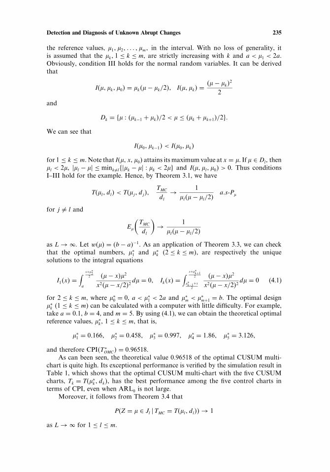
the reference values, �1� �2� � � � � �m� in the interval. With no loss of generality, itis assumed that the �k� 1 ≤ k ≤ m, are strictly increasing with k and a < �1 < 2a.Obviously, condition III holds for the normal random variables. It can be derivedthat

I�� �k� �0� = �k� − �k/2�� I�� �k� =� − �k�

2

2

and

Dk = �� � �k−1 + �k�/2 < � ≤ �k + �k+1�/2��

We can see that

I�0� �k−1� < I�0� �k�

for 1 ≤ k ≤ m. Note that I�� x� �0� attains its maximum value at x = �. If � ∈ Dl, then�l < 2�, ��l − �� ≤ mink �=l���k − �� � �k < 2�� and I�� �l� �0� > 0. Thus conditionsI–III hold for the example. Hence, by Theorem 3.1, we have

T�l� dl� < T�j� dj��TMC

dl

→ 1�l� − �l/2�

a�s-P�

for j �= l and

E�

(TMC

dl

)→ 1

�l� − �l/2�

as L → . Let w�� = b − a�−1. As an application of Theorem 3.3, we can checkthat the optimal numbers, �∗

1 and �∗k 2 ≤ k ≤ m�, are respectively the unique

solutions to the integral equations

I1x� =∫ x+�∗2

2

a

� − x��2

x2� − x/2�2d� = 0� Ikx� =

∫ x+�∗k+12

�∗k−1+x

2

� − x��2

x2� − x/2�2d� = 0 (4.1)

for 2 ≤ k ≤ m, where �∗0 = 0, a < �∗

1 < 2a and �∗m < �∗

m+1 = b. The optimal design�∗k 1 ≤ k ≤ m� can be calculated with a computer with little difficulty. For example,

take a = 0�1, b = 4, and m = 5. By using (4.1), we can obtain the theoretical optimalreference values, �∗

k, 1 ≤ k ≤ m, that is,

�∗1 = 0�166� �∗

2 = 0�458� �∗3 = 0�997� �∗

4 = 1�86� �∗5 = 3�126�

and therefore CPIT ∗OMC� = 0�96518.

As can been seen, the theoretical value 0�96518 of the optimal CUSUM multi-chart is quite high. Its exceptional performance is verified by the simulation result inTable 1, which shows that the optimal CUSUM multi-chart with the five CUSUMcharts, Tk = T�∗

k� dk�, has the best performance among the five control charts interms of CPI, even when ARL0 is not large.

Moreover, it follows from Theorem 3.4 that

PZ = � ∈ Jl �TMC = T�l� dl�� → 1

as L → for 1 ≤ l ≤ m.

236 Han and Tsung

Table 1. Comparisons of the ARLs of the CUSUM, EWMA, GLR, EWMA multi-chart,CUSUM multi-chart, and optimal CUSUM multi-chart with ARL0 = 500

Shifts CUSUM CUSUM Optimal CUSUM EWMA EWMA GLRTGL�(�) � = 1 Multi-chart Multi-chart r = 0�1 Multi-chart d = 3�497

0 500.0(449) 499.5(403) 499.8(477) 500.0(493) 500.3(492) 500.7(490)0.1 372(312) 262(171) 273(228) 320.9(313) 376.6(373) 326.2(290)0.25 145(139) 96.3(57) 96.6(61) 106.5(96) 148.4(139) 113.6(83)0.5 38.5(32) 36.1(21) 35.7(20) 31.25(22) 40.0(31) 36.9(23)0.75 17.3(11) 18.4(10) 19.0(10) 15.87(9) 18.4(12) 18.6(11)1 10.2(6) 11.5(6) 11.9(6) 10.3(5) 11.2(6) 11.4(6)1.25 7.43(3) 8.05(4) 8.21(4) 7.65(3) 7.79(4) 7.79(4)1.5 5.80(2) 6.02(3) 6.07(3) 6.09(2) 5.85(3) 5.75(3)2 4.05(1) 3.81(2 3.79(2) 4.36(1) 3.69(2) 3.61(2)3 2.62(0.9) 2.20(0.8) 2.00(0.9) 2.87(0.7) 1.94(0.9) 1.94(0.8)4 1.99(0.4) 1.56(0.8) 1.34(0.5) 2.19(0.4) 1.28(0.5) 1.32(0.5)

CPI 0.772 0.867 0.880 0.813 0.827 0.870

Example 4.2. Let Xn� n = 1� 2� � � � � be i.i.d. with an exponential distribution withparameter � > 0. Assume that the prechange mean is 1/�0 and the possible intervalof the mean shift is �1/b� 1/a�, where b > a > 0. Without loss of generality, wechoose the reference values, �k (1 ≤ k ≤ m), in �a� b� such that 0 < �0 < �k−1 < �kfor 1 ≤ k ≤ m. Let 1/� ∈ �1/b� 1/a� be an unknown mean shift. It can be calculatedthat

I�� �k� =�k�

− 1− log�k��

I�� �k� �0� =�0 − �k�

�+ log

�k�0�

and

Dk ={� �

�k − �k−1

log �k − log �k−1

< � ≤ �k+1 − �klog �k+1 − log �k

}�

It can be checked that

I�0� �k−1� < I�0� �k�� I�� �k� �0� > 0

for � ∈ Dk� 1 ≤ k ≤ m. Moreover, the example satisfies condition III if � < �0. Thus,the results in Theorems 3.1–3.4 hold for the example.

4.2. Comparisons with Numerical Simulation Results

To compare the detection performance, numerical simulation results of ARLs of thetwo-sided CUSUM, EWMA, CUSUM multi-chart, EWMA multi-chart, and GLRcharts are presented in Table 1. The numerical results of ARLs were obtained basedon 1,000,000-repetition experiments. The common ARL0 here is chosen to be 500,

Detection and Diagnosis of Unknown Abrupt Changes 237

which is a typical value in practice. We compare the simulation results for 10 meanshifts (�1 = 0�1� �2 = 0�25� � � � � �10 = 4) listed in the first column of Table 1 withchange point � = 1. The values in parentheses in every column of the tables are thestandard deviations of the ARLs.

The simulation results of the ARL�’s of the CUSUM chart are listed in thesecond column of Table 1, that is, T�� d� with the reference value � = 1 and thecontrol limit d = 5�075 such that ARL0T1� 5�075�� = 500. The CUSUMmulti-chartresults are listed in the third column, where the CUSUM multi-chart, TMC , consistsof five CUSUM charts, T�k� dk�, 1 ≤ k ≤ 5 with �1 = 0�1, �2 = 0�5, �3 = 1, �4 = 1�5,and �5 = 2. To maintain the overall ARL0TMC� = 500, we choose their controllimits to be d1 = 2�4546, d2 = 5�2217, d3 = 6�017, d4 = 6�2572, and d5 = 6�2789so that ARL0T�1� d1�� = 1500�0, ARL0T�2� d2�� = 1500�0, ARL0T�3� d3�� =1500�0, ARL0T�4� d4�� = 1500�0, and ARL0T�5� d5�� = 1500�0.

The simulation results for the optimal CUSUM multi-chart, T ∗OMC , are listed in

the fourth column with reference values, �∗k, which are determined by (4.1), that

is, �∗1 = 0�166� �∗

2 = 0�458� �∗3 = 0�997� �∗

4 = 1�86, and �∗5 = 3�126, where the control

limits, d1 = 3�64� d2 = 5�24� d3 = 6�17� d4 = 6�45, and d5 = 6�192 are taken in orderto obtain ARL0T

∗OPM� = 500. Also, the simulation results of ARLs for the EWMA

chart, TEr� d�with the parameter r = 0�1 and control limit d = 2�818, and the EWMAmulti-chart, TME� are listed, respectively, in the fifth and the sixth columns, whereTME consists of five EWMA charts, TErk� dk�� 1 ≤ k ≤ 5, with r1 = 0�1� r2 = 0�3,r3 = 0�5� r4 = 0�7, and r5 = 0�9� Similarly, we choose the control limits, dk� 1 ≤ k ≤5, in order to maintain ARL0TME� = 500.

Moreover, we list the simulation results of the GLR(TGL) in the last column withthe control limit d = 3�497, which leads to the same ARL0 value. We take w�� =1/3�9, � ∈ �0�1� 4� for CPI. The bottom row of Table 1 lists the CPI values, whichwere calculated based on all the mean shifts listed in the first column to representthe performance for a range of unknown mean shifts.

Table 1 shows that each charting scheme has its strengths and weaknesses overthe range, and it is difficult to compare them in terms of ARL. However, in termsof CPI for the overall performance, we can see that the optimal CUSUM multi-chart is superior to the CUSUM, CUSUM multi-chart, EWMA, EWMA multi-chart, and GLR charts on the whole in detecting various mean shifts in the range.An interesting result in Table 1 is that the standard deviations of the ARLs for theCUSUM multi-chart and the optimal CUSUM multi-chart are smaller than thosefor the other charts in detecting small mean shifts.

5. CONCLUSIONS AND DISCUSSIONS

Although we rarely know the exact change of a process before detection, we mayassume that the possible unknown postchange �f�� belongs to a known closeddomain D�. In this case we consider a CUSUM multi-chart scheme that consistsof multiple CUSUM control charts for detecting and diagnosing the unknownabrupt change. It is proved that the CUSUM multi-chart not only has a highdiagnostic capability but also has better performance than using individual CUSUMcharts in detecting an unknown abrupt change when the in-control ARL is large.Comparisons of numerical simulation results show that the optimal CUSUMmulti-chart has the best performance according to the CPI values among the five

238 Han and Tsung

schemes, CUSUM, EWMA, CUSUM multi-chart, EWMA multi-chart, and GLRcharts, in detecting various mean shifts. As can be seen, the Kullback–Leiblerinformation distance and the generalized Kullback–Leibler information distanceplay an important role in evaluating not only the detection performance but alsothe diagnostic capability of the multi-chart.

There are still several issues regarding the multi-chart that merit furtherresearch. First, we can see that the main results for the CUSUM multi-chart arebased on the assumption that the constituent charts of the CUSUM multi-charthave a common ALR0. It would be of interest to study whether the same results stillhold for the CUSUM multi-chart when its constituent charts have different ALR0’s.Note that if the small mean shift is considered to be more important than the largeone, the ALR0 of the control chart for a small mean shift may be chosen to besmaller than that of the control chart for a large mean shift, so that the small meanshift can be detected more quickly.

In this paper the comparisons of the detection performance of the control chartsare based on the ARL. Another interesting alternative would be to compare thecharts using the average delay as a criterion. Let N denote the number of falsealarms before the change time � and ��i� for 1 ≤ i ≤ N + 1 be the consecutive alarmintervals until the detection of the change point. Thus,

�1 + · · · + �N < � ≤ �1 + · · · + �N + �N+1�

The average delay time for � = t is thus

ADTt� = Et��1 + · · · + �N+1 − t��

where Et�·� denotes the expectation when the place of shift is at a fixed time t.When t = 0, it becomes the out-of-control ARL ARL� = ADT0�. Srivastava andWu (1993) have used the so-called stationary average delay time, limt→ ADTt�, asthe main measure for evaluating the performance of a detecting procedure.

Usually, the number and position of the reference parameters �1� � � � � �m will beincreased and more scattered in order to keep TMC to have an effective detectionperformance when the domain D becomes large. This case is also true for theoptimal parameters �∗

1� � � � � �∗m. As has been seen, the number of the reference

parameters in the paper is fixed. So, it is interesting to study the influence of a(much) larger D on the results. Also, it is known that, in many practical applications,the i.i.d. assumption does not hold. Thus, it is worthwhile to extend the theorems inthis paper to non-i.i.d. situations such as autocorrelated processes. Such extensionsshould enhance the potential applications of the multi-chart.

APPENDIX: PROOFS OF THE LEMMAS AND THEOREMS

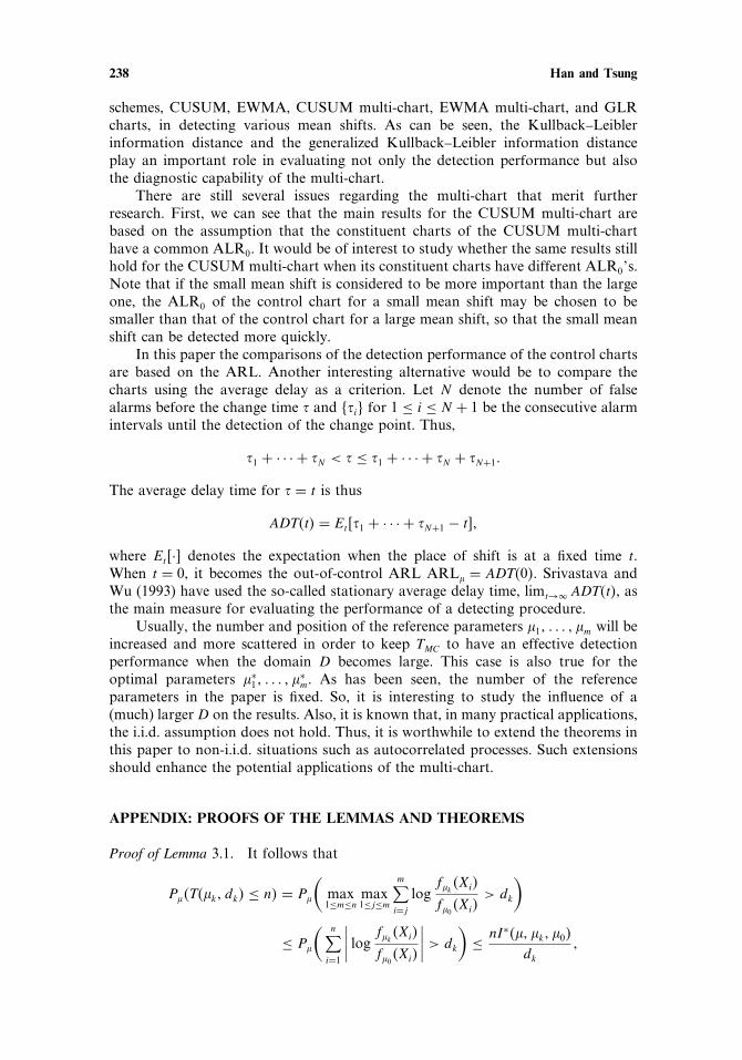
Proof of Lemma 3.1. It follows that

P�T�k� dk� ≤ n� = P�

(max1≤m≤n

max1≤j≤m

m∑i=j

logf�kXi�

f�0Xi�> dk

)

≤ P�

( n∑i=1

∣∣∣∣ log f�kXi�

f�0Xi�

∣∣∣∣ > dk

)≤ nI∗�� �k� �0�

dk

�

Detection and Diagnosis of Unknown Abrupt Changes 239

where the last inequality is obtained by using Markov’s inequality and

I∗�� �k� �0� = E�

∣∣∣∣ log f�kX�

f�0X�

∣∣∣∣�Obviously, P�T�k� dk� ≤ n� converges to zero as dk → since, by condition III,I∗�� �k� �0� < for � ∈ D and 1 ≤ k ≤ m. Thus, T�k� dk� → in probability asdk → . This implies that a subsequence of the T�k� dk�’s goes to infinity a.s.-P�.It is obvious that T�k� dk� is nondecreasing a.s.-P� as each of the dk’s increase toinfinity. This means that T�k� dk� → a.s.-P� as dk → . Thus, the first part (a)of the lemma is proved. Let

N�k� dk� = min{n �

n∑i=1

logf�kXi�

f�0Xi�> dk

}�

It is clear that T�k� dk� ≤ N�k� dk�. Thus, the uniform integrability of�T�k� dk�/dk� dk ≥ 1� follows from the well-known uniform integrability of�N�k� dk�/dk� (for the proof of the latter see, for example, Gut, 1988). �

Proof of Theorem 3.1. We first prove that T�k� dk� < T�l� dl� a.s.-P� as L → forf� ∈ k and l �= k. It is known that (see Siegmund, 1985, p. 26)

L = E�0T�k� dk�� =

edk − 1− dk

I�0� �k�� (A.1)

Thus, we have

dk = dl + Ck� l�+ o1�� logL = dk − log I�0� �k�+ o1� (A.2)

for large L, where

Ck� l� = logI�0� �k�

I�0� �l��

From (A.1) we know that L → if and only if min1≤k≤m�dk� → . By condition Iand (A.2) it follows that dk < dl when k < l since Ck� l� < 0 for k < l.

By condition II we know that f� ∈ k means that I�� �k� �0� ≥ I�� �l� �0� forl �= k and I�� �k� �0� > 0. Assume that I�� �k� �0� > I�� �l� �0� for l �= k. By thestrong law of large numbers we have

max1≤j≤n

1n

n∑i=j

logf�lXi�

f�0Xi�→ max�0� I�� �l� �0��� a.s.-P� (A.3)

for 1 ≤ l ≤ m as n → . Writing Tj = T�j� dj�� 1 ≤ j ≤ m for short, we have

max1≤j≤Tl

Tl∑i=j

logf�lXi�

f�0Xi�> dl

and

max1≤j≤Tk−1

Tk−1∑i=j

logf�kXi�

f�0Xi�≤ dk�

240 Han and Tsung

It follows from (A.2) that

max1≤j≤Tl

1Tl

Tl∑i=j

logf�lXi�

f�0Xi�>

dl

Tl

= dk

Tl

+ Cl� k�+ o1�Tl

≥ Tk − 1Tl

max1≤j≤Tk−1

1Tk − 1

Tk−1∑i=j

logf�kXi�

f�0Xi�+ Cl� k�+ o1�

Tl

�

(A.4)

Note that Cl� k�/Tl → 0� a.s.-P� as L → . By (A.3), (A.4), and Part (a) ofLemma 3.1, we have

max�0� I�� �l� �0�� ≥Tk − 1Tl

I�� �k� �0��

a.s.-P� as L → . This means that Tk < Tl, a.s.-P� as L → for l �= k sinceI�� �k� �0� > I�� �l� �0��

Let I�� �k� �0� = I�� �l� �0�, that is, I�� �k� = I�� �l�. By the definition of the’s we know that if f� ∈ k and I�� �k� = I�� �l�, it must have l > k. For instance,f� can only belong to the boundary of k and k+1, not to the boundary of k andk−1 when f� ∈ k. Note that

max1≤j≤Tk

1Tk

Tk∑i=j

logf�kXi�

f�0Xi�>

dk

Tk

and

max1≤j≤Tk−1

1Tk − 1

Tk−1∑i=j

logf�kXi�

f�0Xi�≤ dk

Tk − 1�

By the strong law of large numbers, this implies that

Tk/dk →1

I�� �k� �0�a.s.-P��

as L → . Similar result can be obtained for Tl. Thus T�k� dk� < T�l� dl�, a.s.-P��since dk > dl and

T�k� dk�

dk

→ 1I�� �0�− I�� �k�

= 1I�� �0�− I�� �l�

← T�l� dl�

dl

a.s.-P� as L → .Since T�k� dk� < T�l� dl� a.s.-P� as L → it follows that TMC − T�k� dk� → 0

a.s.-P� as L → , and therefore,

TMC

dk

→ 1I�� �k� �0�

a.s.-P�

as L → . Note that the family �TMC/dk� dk > 0� is uniformly integrable withrespect to P� since TMC ≤ T�k� dk�, and �T�k� dk�/dk� dk > 0� is uniformly

Detection and Diagnosis of Unknown Abrupt Changes 241

integrable with respect to P�. Thus, by application of Theorem A.1.1 in Gut (1988),we have

E�

(TMC

dk

)→ 1

I�� �k� �0�

as L → . �

Proof of Lemma 3.2. We first show that Lemma 3.2 holds for m = 2. By (3.4), (A.1),and (A.2), we have

d′i − d′

j = 1+ o1��di − dj� = 1+ o1��[ln(IiIj

)](A.5)

for large L. It follows that

L′ − L = E�0T�1� d

′1��− E�0

T ′MC�

=+∑n=0

{P�0

(T�1� d

′1� > n

)− P�0

(T�i� d

′i� > n� 1 ≤ i ≤ 2

)}

=+∑n=1

P�0

(T�2� d

′2� ≤ n� T�1� d

′1� > n

)�

Writing T ′i = T�i� d

′i�� i = 1� 2, and P·� = P�0

·�� E·� = E�0·� in short, T ′

i can beexpressed by (see Siegmund, 1985, p. 25)

T ′i = N

i�1 + N

i�2 + · · · + N

i�

Ki� (A.6)

and

ET ′i � = EN

i�1 �EKi��

where Si�n =∑n

j=1 log�f�i Xj�/f�0Xj��,

Ni�1 = inf

{n � Si�

n � 0� d′i�}� N

i�k = inf

{n ≥ 1 � S

i�N1+···+Nk−1+n − S

i�N1+···+Nk−1

� 0� d′i�}�

and

Ki� = inf{k � S

i�

Ni�1 +···+N

i�k

− Si�

Ni�1 +···+N

i�k−1

≥ d′i

}�

Moreover,{N

i�k � k ≥ 1

}is i.i.d. with mean E

(N

i�1

)and Ki� is geometrically distri-

buted with mean EKi�� = 1/P(Si�

Ni�1

≥ d′i

). Note that E

(Si�1

) = −Ii = −I�0� �i� < 0.

We can further prove that there exists � > 0 such that

E(e�N

i�1)< (A.7)

for i = 1� 2. In fact, by condition III and Chebyshev’s inequality it follows that

e�nIiP(Si�n + nIi ≥ nIi

) ≤ E(e�S

i�n +nIi

) = h��n

242 Han and Tsung

where hi�� = E(e�log�f�i Xj�/f�0 Xj��+Ii�

). Taking small positive � such that Ii�−

log hi�� > 0, we have

P(N

i�1 > n

) ≤ P(Si�n ≥ 0

) = P(Si�n + nIi ≥ nIi

) ≤ e−nIi�−log hi����

This implies that (A.7) holds for Ni�1 . Obviously 1 ≤ E

(N

i�1

)< , i = 1� 2� Let pi =

P(Si�

Ni�1

≥ d′i

), Ei = E

(N

i�1

)and f1�� = E

(e�N

1�1 −E1�

)and f2�� = E

(e�−N

2�1 +E2�

). Set

n′ = d′1e

d′1/I1E1�� n1 = n/E1 + ��, and n2 = n/E2 − �� for small �0 < � < 1�. Itfollows from (A.6) that

+∑n=1

P(T ′2 ≤ n� T ′

1 > n) ≤ n′∑

n=1

P(T ′2 ≤ n� T ′

1 > n)+ +∑

n=n′+1

P(T ′1 > n

) = Qd′1� d

′2�+Qd′

1�

where

Qd′1� d

′2� =

n′∑n=1

∑k=1

∑j=1

p21− p2�k−1p11− p1�

j−1

× P(N

2�1 + · · · + N

2�k ≤ n�N

1�1 + · · · + N

1�j > n

)and

Qd′1� =

∑n=n′+1

∑j=1

p11− p1�j−1P

(N

1�1 + · · · + N

1�j > n

)�

Taking � such that � < � and ai�� = ��− log fi�� > 0 for i = 1� 2, we have (byChebyshev’s inequality)

P

( k∑l=1

N2�l ≤ n

)= P

( k∑l=1

−N2�l + kE2 ≥ kE2 − n/k�

)

≤ exp�−k�E2 − n/k��− log f2���� ≤ exp�−ka2���

for k > n2. Similarly,

P

( j∑l=1

N1�l ≥ n

)= P

( j∑l=1

N1�l − jE1 ≥ jn/j − E1�

)

≤ exp�−j�n/j − E1��− log f1���� ≤ exp�−ja1���

for j ≤ n1. Thus

Qd′1� d

′2� ≤

n′∑n=1

{ ∑k=n2+1

p21− p2�k−1P

( k∑l=1

N2�l ≤ n

)

+n1∑j=1

p11− p1�j−1P

( j∑l=1

N1�l > n

)}

+n′∑n=1

{ n2∑k=1

∑j=n1+1

p21− p2�k−1p11− p1�

j−1

}

Detection and Diagnosis of Unknown Abrupt Changes 243

≤n′∑n=1

{ ∑k=n2+1

p21− p2�k−1e−ka2�� +

n1∑j=1

p11− p1�j−1e−ja1��

}

+n′∑n=1

�1− 1− p2�n2 �1− p1�

n1

≤n′∑n=1

{p21− p2�e

−a2���n2+1

1− p2�1− 1− p2�e−a2���

+ p11− p1�e−a1���1− �1− p1�e

−a1���n1�

1− p1�1− 1− p1�e−a1���

}+ Pd′

1� d′2�

≤ n′p2

1− p2�1− 1− p2�e−a2���

+ n′p1

1− p1�1− 1− p1�e−a1���

+ Pd′1� d

′2�

where

Pd′1� d

′2� =

n′∑n=1

�1− 1− p2�n2 �1− p1�

n1

= 1− p1�1

E1+� 1− 1− p1�n′

E1+� �

1− 1− p1�1

E1+�

− 1− p1�1

E1+� 1− p2�1

E2−� �1− 1− p1�n′

E1+� 1− p2�n′

E2−� �

1− 1− p1�1

E1+� 1− p2�1

E2−�

�

Note that

pi = PSi�

Ni�1

≥ d′i� =

Ei

ET ′i �

= EiIie−d′i 1+ Od′

ie−d′i ��

for i = 1� 2� and d′2 − d′

1 = 1+ o1�� logI2/I1�� n′p2 ≤ d′

1I2E2/I1E1�e−d′2−d′1� ≤

d′1E2/E1, and n′p1 = d′

1 + o1�. Furthermore,

1− 1− p1�1

E1+� → I1E1e−d′1/E1 + ��� 1− 1− p2�

1E2−� → I2E2e

−d′2/E2 − ��

and

1− p1�n′

E1+� ∼ Oe−d′1� → 0� 1− p2�n′

E2−� ∼ Oe−d′1� → 0

as d′i → � i = 1� 2� We have

Pd′1� d

′2� =

1− p1�1

E1+�

(1− 1− p2�

1E2−�

)[1− 1− p1�

1E1+�

][1− 1− p1�

1E1+� 1− p2�

1E2−�

] + O1�

= ed′1

I1

(E1 + �

E1

1

1+ E2−�

E2

E1E1+�

+ Oe−d′1�

)

= ed′1

I1

[12+ O��+ Oe−d′1�

]= L′

[12+ O��+ Oe−d′1�

]

244 Han and Tsung

for large d′1 or L

′ and small �. Thus

Qd′1� d

′2� ≤ L′

[12+ O��+ Oe−d′1�+ Od′

1/L′�]�

Next we estimate Qd′1�. Taking �a� such that a = f ′

1�a��/f1�a�� for a > E1,it follows that a = f ′

1��/f1�� is strictly increasing (see Durrett, 1996, pp. 71–73), so that �E1� = 0, �E1 + �� > 0 and therefore log f1�E1 + ��� > 0. Further,the function gx� = �x�− x−1 log f1�x�� is increasing for x ≥ E1 since g′x� =x−2 log f1�x�� ≥ 0 for x ≥ E1 and gE1� = 0. Thus

P(N

1�1 + · · · + N

1�j > jn/j�

) ≤ exp�−j�n/j��n/j�− log f1�n/j����

= exp{− n

[�n/j�− j

nlog f1�n/j��

]}

≤ exp{− n

[�E1 + ��− 1

E1 + �log f1�E1 + ���

]}

= e−ngE1+���

for j ≤ n1 = n/E1 + ��. Hence

Qd′1� ≤

∑n=n′+1

{ n1∑j=1

p11− p1�j−1P

(N

1�1 + · · · + N

1�j > n

)+

∑j=n1+1

p11− p1�j−1

}

≤∑

n=n′+1

1− 1− p1�n1�e−ngE1+�� +

∑n=n′+1

1− p1�n1

≤ e−n′+1�gE1+��

1− e−gE1+��+ 1

p1

1− p1�n′+1 = 1

I1E1

+ o1�

for large d′1. Thus we have

L′ − L = E�0T�1� d

′1��− E�0

T ′MC� ≤ Qd′

1� d′2�+Qd′

1�

≤ L′(12+ O��+ Oe−d′1�+ O1/L′�+ Od′

1/L′�)

for large L. This implies that L′/L ≤ 2+ o1� for large L. It follows from (3.4) and(A.1) that L′/L = ed

′i−di + o1�. Thus, d′

i − di ≤ log 2+ o1� for large L.For m ≥ 3 we define T

k�MC = min1≤j≤k�T�j� d

′j�� for 1 ≤ k ≤ m. Since T

1�MC =

T�1� d′1� and T

m�MC = T ′

MC , it follows that

L′ − L = E�0T�1� d

′1��− E�0

T ′MC� =

m−1∑k=1

(E�0

Tk�MC�− E�0

Tk+1�MC �

)�

Note that

E�0

(T

k�MC�− E�0

Tk+1�MC

)=

+∑n=0

P(T�k+1� d

′k+1� ≤ n� T�j� d

′j� > n� 1 ≤ j ≤ k

)

≤n′∑n=1

P(T�k+1� d

′k+1� ≤ n� T�j� d

′j� > n� 1 ≤ j ≤ k

)+Qd′1��

Detection and Diagnosis of Unknown Abrupt Changes 245

We can similarly prove that

n′∑n=1

P(T�k+1� d

′k+1� ≤ n� T�j� d

′j� > n� 1 ≤ j ≤ k

)

≤ n′pk+1

1− pk+1�1− 1− pk+1�e−ak+1���

+k∑

j=1

n′pj

1− pj�1− 1− pj�e−aj���

+ Pd′1� � � � � d

′k+1�

and

P(d′1� � � � � d

′k+1

)=

n′∑n=1

�1− 1− pk+1�nk+1 �

k∏j=1

1− pj�nj

=∏k

j=11− pj�1

Ej+�

[1− 1− pk+1�

1Ek+1−�

][1−∏k

j=11− pj�1

Ej+�

][1− 1− pk+1�

1Ek+1−�

∏kj=11− pj�

1Ej+�

] + O1�

= ed′1

I1

(1∑k

j=1Ej

Ej+�

1(1+ Ek+1−�

Ek+1

∑kj=1

Ej

Ej+�

) + o1�

)

= L′(

1kk+ 1�

+ O��+ o1�)

for large d′1 or L′ and small �, where pj = P

(Sj�

Nj�1

≥ d′j

), nj = n/Ej + ��� 1 ≤ j ≤ k,

and nk+1 = n/Ek+1 − ��. Thus

L′ − L ≤ L′( m−1∑

k=1

1kk+ 1�

+ O��+ o1�)= L′

(1− 1

m+ O��+ o1�

)�

and therefore L′/L ≤ m+ o1� and d′k − dk ≤ logm+ o1�� 1 ≤ k ≤ m� for large L.

This completes the proof of Lemma 3.2. �

Proof of Theorem 3.2. Let f� ∈ D�. Without loss of generalization, we assumef� ∈ k. This means that I�� �k� �0� ≥ I�� �i� �0� for i �= k and I�� �k� �0� > 0.By the condition of Theorem 3.2, there is �l ∈ Dll �= k� such that I�� �k� �0� >I�� �l� �0�. Let Tj = T�j� dj�� 1 ≤ j ≤ m� and

Yldl� = max1≤j≤Tl

1Tl

Tl∑i=j

logf�lXi�

f�0Xi��

It follows from (A.4) that

Tl >dl

Yldl�> 0

246 Han and Tsung

and therefore

E�

(Tl − Tk�

dk

)≥ E�

(dl

dkYldl�

)− E�

(Tk

dk

)�

Note that dl/dk → 1,

E�

(Tk

dk

)→ 1

I�� �k� �0��

and

Yldl� → max�0� I�� �l� �0��� a.s.-P�

as L → . Here, L → if and only if min1≤k≤m�dk� → . Thus, by Fatou’s lemmawe have

lim infL→

E�

(Tl − Tk�

dk

)≥ 1

max�0� I�� �l� �0��− 1

I�� �k� �0�

= 1I�� �k� �0�

(I�� �k� �0�

max�0� I�� �l� �0��− 1

)

and therefore

lim infL→

E�

(Tl − Tk�

dk

)={+ if I�� �l� �0� ≤ 0�

I���k��0�−I���l��0�

I���k��0�I���l��0�if I�� �l� �0� > 0�

Taking c > 0 such that c < I�� �k� �0� and letting

cl =I�� �k� �0�−max�c� I�� �l� �0��

I�� �k� �0�max�c� I�� �l� �0���

we have

E�Tl − Tk�/dk� ≥ cl > 0

for large L.If there is l such that I�� �l� �0� = I�� �k� �0�, by the definition of the divide

domains, j� 1 ≤ j ≤ m, we know that it must have l > k, and therefore (see theproof of Theorem 3.1) dl > dk. Defining a set Ak, every j ∈ Ak satisfies j > k andI�� �j� �0� = I�� �k� �0�. The set Ak may be empty if there is no j such thatI�� �j� �0� = I�� �k� �0�. Let �Ak = �1� � � � � m�− Ak. Similarly, we have

E�Tl − Tk�/dk� ≥ cl > 0

for l ∈ �Ak and large L.On the other hand, by Lemma 3.2 and (3.3) of Theorem 3.1 we have d′

i − di ≤logm, d′

i/di → 1 for 1 ≤ i ≤ m, and

�E�T�k� dk��− E�T�k� d′k���

dk

= E�T�k� dk��

dk

− d′k

dk

E�T�k� d′k��

d′k

→ 1I�� �k� �0�

− 1I�� �k� �0�

= 0

Detection and Diagnosis of Unknown Abrupt Changes 247

as L → . Similarly, we have (see the proof of Theorem 3.1)

E�Tj/dj� →1

I�� �j� �0�� E�Tj − Tk�/dk� → 0

for j ∈ Ak as L → since I�� �j� �0� = I�� �k� �0� and dj/dk → 1 as L → . Notethat E�T�k� d

′k�� ≥ E�T

′MC�. Thus

1dk

[ m∑l=1

plE�T�l� dl��− E�T′MC�

]

= 1dk

m∑l=1

pl�E�T�l� dl��− E�T�k� dk���+1dk

�E�T�k� dk��− E�T′MC��

= 1dk

∑l∈Ak

pl�E�T�l� dl��− E�T�k� dk���

+ 1dk

∑j∈Ak

pj�E�T�j� dj��− E�T�k� dk���

+ 1dk

�E�T�k� dk��− E�T�k� d′k��+ E�T�k� d

′k��− E�T

′MC��

≥ ∑l∈Ak

plcl + o1� > 0

for large L, and therefore,

m∑l=1

plE�T�l� dl�� > E�T′MC�

for large L. �

ACKNOWLEDGMENTS

We thank the special issue guest editor and two referees for their valuable commentsand suggestions, which have improved this work. We are especially grateful toa referee who pointed out a mistake in an earlier proof of Lemma 3.1. Wealso thank Yanting Li for her help in the numerical simulations. This work wassupported by RGC Competitive Earmarked Research Grants HKUST6232/04Eand HKUST6204/05E.

REFERENCES

Baxley, R. V., Jr. (1995). An Application of Variable Sampling Interval Control Charts,Journal of Quality Technology 27: 275–282.

Box, G. E. P. and Luceño, A. (1997). Statistical Control by Monitoring and FeedbackAdjustment, New York: Wiley.

Crowder, S. V. (1987). A Simple Method for Studying Run Length Distributions ofExponentially Weighted Moving Average Control Charts, Technometrics 29: 401–407.

248 Han and Tsung

Crowder, S. V. (1989). Design of Exponentially Weighted Moving Average Schemes, Journalof Quality Technology 21: 155–162.

Dragalin, V. (1993). The Optimality of Generalized CUSUM Procedure in QuickestDetection Problem, Proceedings of Steklov Institute of Mathematics: Statistics and Controlof Stochastic Processes 202: 132–148.

Dragalin, V. (1997). The Design and Analysis of 2-CUSUM Procedure, Communications inStatistics—Simulation & Computation 26: 67–81.

Durrett, R. (1996). Probability Theory and Examples, 2nd ed., Belmont: Wadsworth.Gut, A. (1988). Stopping Time Random Walks: Limit Theorems and Applications, New York:

Springer.Han, D. and Tsung, F. G. (2004). A Generalized EWMA Control Chart and Its Comparison

with the Optimal EWMA, CUSUM and GLR Schemes, Annals of Statistics 32:316–339.

Hawkins, D. M. and Olwell, D. H. (1998). Cumulative Sum Charts and Charting for QualityImprovement, New York: Springer.

Jiang, W., Tsui, K. L., and Woodall, W. H. (2000). A New SPC Monitoring Method: TheARMA Chart, Technometrics 42: 399–416.

Jones, L. A., Champ, C. W., and Rigdon, S. T. (2001). The Performance of ExponentiallyWeighted Moving Average Charts with Estimated Parameters, Technometrics 43: 156–167.

Lai, T. L. (1995). Sequential Change-Point Detection in Quality Control and DynamicSystems, Journal of Royal Statistical Society, Series B 57: 613–658.

Lai, T. L. (1998). Information Bounds and Quick Detection of Parameter Changes inStochastic Systems, IEEE Transactions on Information Theory 44: 2917–2929.

Lai, T. L. and Shan, J. Z. (1999). Efficient Recursive Algorithms for Detection for AbruptChanges in Signals and Control Systems, IEEE Transactions on Automatic Control 44:952–966.

Lorden, G. (1971). Procedures for Reacting to a Change in Distribution, Annals ofMathematical Statistics 42: 1897–1908.

Lorden, G. and Eisenberger, I. (1973). Detection of Failure Rate Increases, Technometrics15: 167–175.

Lucas, J. M. and Saccucci, M. S. (1990). Exponentially Weighted Moving Average ControlSchemes: Properties and Enhancements, Technometrics 32: 1–16.

Luceño, A. (1999). Average Run Lengths and Run Length Probability Distributions forCuscore Charts to Control Normal Mean, Computational Statistics and Data Analysis32: 177–195.

Mastrangelo, C. M. and Brown, E. C. (2000). Shift Detection Properties of MovingCenterline Control Chart Schemes, Journal of Quality Technology 32: 67–74.

Mastrangelo, C. M. and Montgomery, D. C. (1995). SPC with Correlated Observations forthe Chemical and Process Industries, Quality and Reliability Engineering International11: 79–89.

Montgomery, D. C. and Mastrangelo, C. M. (1991). Some Statistical Process Control ChartsMethods for Autocorrelated Data, Journal of Quality Technology 23: 179–193.

Moustakides, G. V. (1986). Optimal Stopping Times for Detecting Changes in Distribution,Annals of Statistics 14: 1379–1387.

Nikiforov, I. (2000). A Suboptimal Quadratic Change Detection Scheme, IEEE Transactionson Information Theory 46: 2095–2107.

Ramírez, G. J. (1998). Monitoring Clean Room Air Using Cuscore Charts, Quality andReliability Engineering International 14: 281–289.

Reynolds, M. R., Jr. (1996a). Shewhart and EWMA Control Charts Using VariableSampling Intervals with Sampling at Fixed Times, Journal of Quality Technology 28:199–212.

Detection and Diagnosis of Unknown Abrupt Changes 249

Reynolds, M. R., Jr. (1996b). Variable Sampling-Interval Control Charts with Sampling atFixed Times, IIE Transactions 28: 497–510.

Ritov, Y. (1990). Decision Theoretic Optimality of the CUSUM Procedure, Annals ofStatistics 18: 1464–1469.

Shiryaev, A. N. (1995). Probability, New York: Springer.Shu, L. J., Apley, D. W., and Tsung, F. (2002). Autocorrelated Process Monitoring Using

Triggered Cuscore Charts, Quality and Reliability Engineering International 18: 411–421.Siegmund, D. (1985). Sequential Analysis: Tests and Confidence Intervals, New York: Springer.Siegmund, D. and Venkatraman, E. S. (1995). Using the Generalized Likelihood Ratio

Statistic for Sequential Detection of a Change-Point, Annals of Statistics 23: 255–271.Sparks, R. S. (2000). CUSUM Charts for Signalling Varying Location Shifts, Journal of

Quality Technology 32: 157–171.Srivastava, M. S. and Wu, Y. H. (1993). Comparison of EWMA, CUSUM and Shiryavev-

Robters Procedures for Detecting a Shift in the Mean, Annals of Statistics 21: 645–670.Willsky, A. S. and Jones, H. L. (1976). A Generalized Likelihood Ratio Approach to

Detection and Estimation of Jumps in Linear Systems, IEEE Transactions on AutomaticControl 21: 108–112.