Detecting Scene ElementsUsing Maximally Stable Colour Regions

Stanislav Basovnik, Lukas Mach, Andrej Mikulik, and David Obdrzalek

Charles University in Prague, Faculty of Mathematics and PhysicsMalostranske namesti 25, 118 00 Praha 1, Czech Republic

sbasovnik@gmail.com, lukas.mach@gmail.com,

andrej.mikulik@gmail.com, david.obdrzalek@mff.cuni.cz

Abstract. Image processing for autonomous robots is nowadays verypopular. In our paper, we show a method how to extract informationfrom a camera attached on a robot to acquire locations of targets therobot is looking for. We apply maximally stable colour regions (a methodoriginally used for image matching) to obtain an initial set of candidateregions. This set is then filtered using application specific filters to findonly the regions that correspond to scene elements of interest. The pre-sented method has been applied in practice and performs well even undervarying illumination conditions since it does not rely heavily on manuallyspecified colour thresholds. Furthermore, no colour calibration is needed.

Keywords. Autonomous robot, Maximally Stable Colour Regions

1 Introduction

Autonomous robots often use cameras as their primary source of informationabout their surroundings. In this work, we describe a computer vision systemcapable of detecting scene elements of interest, which we used for an autonomousrobot. The main goals we try to achieve are robustness of the method and com-putational efficiency.

The core of our vision system are Maximally Stable Extremal Regions, orMSERs, introduced by Matas et. al (see [1]) for gray-scale images and later ex-tended to colour as Maximally Stable Colour Regions, or MSCR (see [2]). Detailsabout MSER and MSCR principles are given in Sections 2 and 3, respectively.

The main usage of MSER detection is for wide-baseline image matchingmainly because of its affine covariance and high repeatability. To match two im-ages of the same scene (taken from different viewpoints), MSERs are extractedfrom both images and then appropriately described using (usually affinely in-variant) descriptor (see [5,6]). Because MSER extraction is highly repeatable,the majority of the regions should be detected in both images. If the descriptoris truly affinely invariant, identical regions should have the same (or similar)descriptors even though they are seen from different viewpoints (assuming theregions correspond to small planar patches in the scene). Then, the matchingcan be done using nearest neighbour search of the descriptors.

In our system, MSCRs are not used for matching but for object detection.The system operates in the following steps:

– Detect large number of contrasting regions in the image.– Classify detected regions and decide which correspond to elements of interest.– Localize detected elements and pass this information to other components

of robot’s software.

MSER and MSCR algorithms often return large number of (possibly overlap-ping) regions. We therefore introduce our classification algorithm which rejectsregions with small probability of corresponding to a scene element of interest.The relative position of the scene element is then determined using standardalgorithms from computer vision and projective geometry [3].

Typical input image and output in the form of list of detected objects canbe seen in Figure 1.

Localization results

object 1 [-0.74, 0.72, 0.01]object 2 [0.84, 1.97, 0.05]object 3 [-0.81, 2.20, -0.01]object 4 [0.23, 3.21, 0.04]

Fig. 1. Input image, detected regions, and final output table – triangulated coordinatesof detected objects.

The following text is structured as follows: We first briefly describe the MSER(Section 2) and MSCR (Section 3) algorithms. In Section 4, we present ourfiltering system which processes the regions and outputs locations of detectedobjects. Section 5 discusses the overall efficiency of the proposed algorithm.

2 MSER

In this section, we describe the MSER algorithm as a basis for our region detec-tion.

The MSER detection uses a watershedding process that can be described inthe following way:

The gray-scale image is represented by function I : Ω → [0..255], whereΩ = [1..W ] × [1..H] is the set of all image coordinates. We choose an intensitythreshold t ∈ [0..255] and divide the set of pixels into two groups B (black) andW (white).

B :=x ∈ Ω2 : I(x) < t

W := Ω2 \B

When changing the threshold from maximum to minimum intensity, the car-dinality of the two sets changes. In the first step, all pixel positions will becontained in B and W is empty (we see completely black image). As the thresh-old t is lowered, white spots start to appear and grow larger. White regions growand eventually all merge when the threshold reaches near minimum intensity andthe whole image will be white (all pixels are in W and B is empty). Figure 2demonstrates the evolution process with different threshold levels.

Fig. 2. MSER evolution of the input image shown in Figure 1. Results of 9 differentthresholding levels are displayed, each time for lower intensity threshold t.

Connected components in these images (white spots and black spots) arecalled extremal regions. Maximally stable regions are those that have changedin size only a little across at least several intensity threshold levels. The numberof levels needed is a parameter of the algorithm.

3 MSCR

In this section, we outline the MSCR method as extension of MSER from gray-scale to colour images (see [2]).

In the following text, we assume the image to be in RGB colour space, butit can be easily seen the MSCR method can work with other colour spaces too.To detect MSCRs, we take the image function I : Ω → R3. Thus, the imagefunction I assigns a colour (RGB channel values) to all pixel positions in thegiven image. We also define graph G, where the vertices are all image pixels, andthe edge set E is defined as follows (note that x, y are 2-dimensional vectors):

E :=x,y ∈ Ω2 : |x− y| = 1

where |x − y| is a Euclidean distance of pixel coordinates x and y (other

metrics, e.g. Manhattan distance, can be considered too). Edges in the graphconnect neighbouring pixels in the image. Every edge is assigned with the weightg(x,y) that measures the colour difference between the neighbouring x and ypixels. In accordance with [2], we use the Chi squared measure to calculate thevalue of g:

g2(x,y) =3∑

k=1

(Ik(x)− Ik(y))2

Ik(x) + Ik(y)

where Ik(x) denotes the value of the k-th colour channel of the pixel x.

(a) (b)

Fig. 3. Blurred input image and first stage of MSCR evolution.

We then consider series of subgraphs Et ⊆ E, where the set Et contains onlyedges with weight ≤ t. The connected components of Et will be referred to asregions. In the MSCR algorithm, we start with Et, t = 0 and then graduallyincrease t. As we do this, new edges appear in the subgraph Et and regionsstart to grow and merge. MSCR regions are those regions that are stable (i.e.,

(a) (b)

Fig. 4. Evolution of regions with increasing threshold.

nearly unchanged in size) across several thresholding levels, similarly to MSERalgorithm.

For an example of detected MSCR regions, refer to Figures 3 and 4: Figure3(a) shows the input image (after it is blurred using Gaussian kernel as is usuallydone in image segmentation to handle the noise). Figure 3(b) shows regions ofthe graph with edges E0 (represented in false colours: different components ofthis graph have different colours, trivial isolated 1 pixel components are black).Figures 4(a) and 4(b) show two further stages of the computation – as we increasethe threshold t, we can see the homogeneous parts of the image merge and formregions. We can see that the contours of important scene elements can be clearlydistinguished on the latter two images.

4 Filtering regions

This section shows how the set of regions detected by MSCR is filtered so thatonly interesting regions are kept and regions without the importance to theapplication are discarded.

Using MSER and MSCR, we retrieve quite large number of image regions (seeFigure 5), of which only a few is of any importance. Therefore, this set of regionshas to be filtered to discard all regions of no interest. This part is applicationspecific and depends on the appearance of the objects that are being detected.In our testcase, the robot operates on a relatively small space with flat singlecoloured surface and it interacts with scene elements of two colours, red andgreen. So, the scene elements have contrasting colours to the background, whichis a standard assumption for successful object detection in a coloured image.

In the following paragraphs, we show the individual filters that were succes-sively applied on the original set of regions. The result is a list of objects, whichis passed for further processing in the robot planning algorithm. Figure 5 showsthe input image and the first set of regions, which is to be filtered, Figure 6shows the situation after each step.

Fig. 5. Input picture and all detected regions denoted by black contour.

4.1 Discarding regions touching image border

A useful heuristic to reject regions detected outside of the working area is todiscard regions touching the image border. Of course, this way we may alsoreject contours that really correspond to important scene element. However,since reliable detection of objects that are only partially visible is considerablyharder, we have decided to reject them without substantial loss. Figure 6(b)shows the regions which remain after dropping regions touching the border. Inthis particular case, no loss of interesting regions occurred.

4.2 Shape classification

After the contour is detected, the polygonal shape is then simplified by usingthe classic Douglas-Peucker algorithm (see e.g. [4]). If the resulting polygon istoo large or too small (above or below specified parameters), it is rejected. Thelower and upper limits are set according to expected size of objects the robotshould detect.

Also, in our case the objects of interest all lie on the ground and their shapecontours contains parallel lines (e.g. a cylinder). Therefore, the detected contoursshould contain long segments that are either horizontally or vertically alignedwith the image coordinate system. If such segment cannot be found, the regionis rejected. Figure 6(c) shows the set of regions after applying this filter.

4.3 Statistical moments (covariance matrix)

Contours corresponding to the top parts of objects can often be nicely andreliably isolated and detected. The column elements, which are used in Eurobot2009, have circular shape and therefore the image of the top part is an ellipse(for details about Eurobot autonomous robot contest, see [7]). We thereforetake special care to distinguish elliptical regions from all others. To do this, wecalculate first, second and third statistical moments of the region. Since ellipseis a second-order curve, its third statistical moment should ideally be zero (in

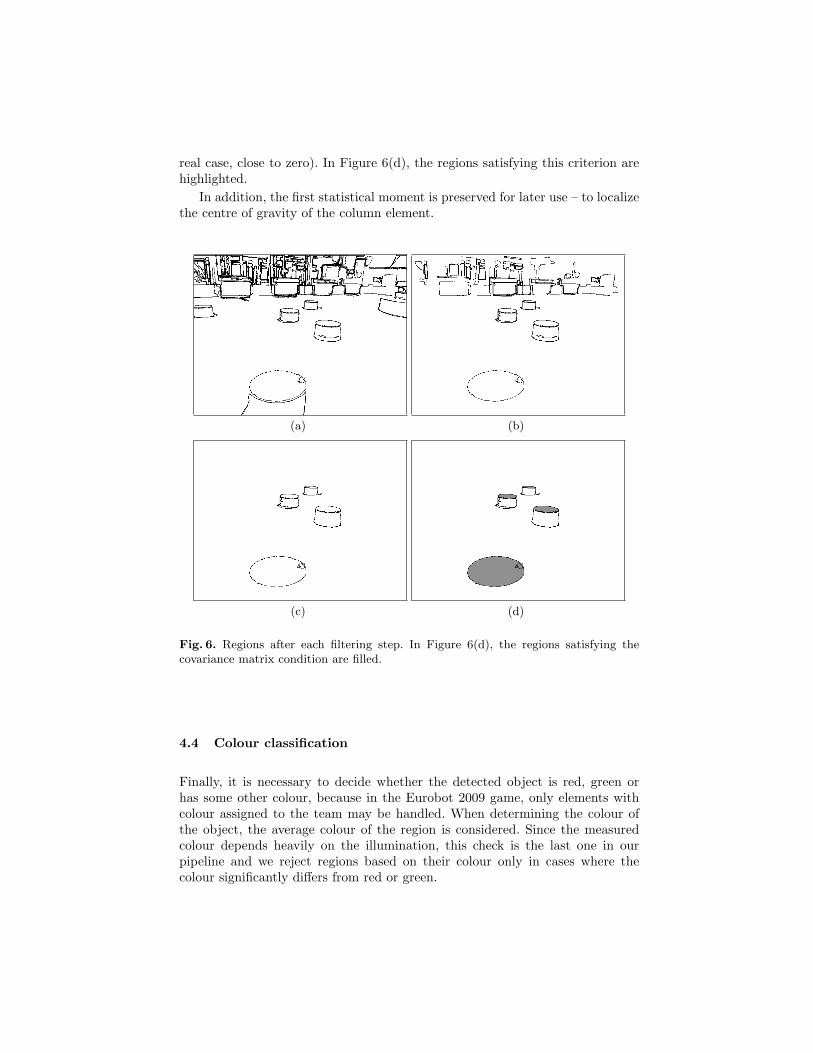
real case, close to zero). In Figure 6(d), the regions satisfying this criterion arehighlighted.

In addition, the first statistical moment is preserved for later use – to localizethe centre of gravity of the column element.

(a) (b)

(c) (d)

Fig. 6. Regions after each filtering step. In Figure 6(d), the regions satisfying thecovariance matrix condition are filled.

4.4 Colour classification

Finally, it is necessary to decide whether the detected object is red, green orhas some other colour, because in the Eurobot 2009 game, only elements withcolour assigned to the team may be handled. When determining the colour ofthe object, the average colour of the region is considered. Since the measuredcolour depends heavily on the illumination, this check is the last one in ourpipeline and we reject regions based on their colour only in cases where thecolour significantly differs from red or green.

4.5 Position calculation

After the regions are filtered and their colour is classified, we calculate theirposition on the playground. It is possible to calculate the object position becausewe know the camera parameters (from its calibration) and we also know thatthe objects lie on the ground. We then save this information into appropriatedata structures and pass it to other components of robot’s software to be usede.g. for navigation.

4.6 Final output

After the filtering, the remaining regions are claimed to represent real objectson the playing field. Figure 1 shows the resulting table of objects. For furtherprocessing, only these coordinates are sent out. This is a very little amount ofdata and at the same time, it is a very good input for the central ”brain” of therobot, which uses this information for example as data for trajectory planningprocess.

5 Computational efficiency

Robots often have limited computational power which restricts the use of com-putationally intensive algorithms. In this section, we discuss the computationalcomplexity of the method.

The (greyscale) MSER algorithm first sorts individual pixels according totheir intensity. Since the pixel intensity is an integer from the interval [0..255],this can be done in O(n) time using radix sort. During the evolution process,regions are merged as new pixels get above the decreasing threshold t. To do this,the regions must be stored in memory in appropriate data structures and a fastoperation for merging two regions has to be implemented. This is straightforwardapplication of the union-find algorithm with time complexity of O(nα(n)), whereα(n) is the inverse Ackermann function – an extremely slowly growing function.Therefore, this part does not bring in real cases significant time demands.

The MSCR variant differs from MSER in two respects. Individual pixels arenot considered; instead the edges between neighbouring pixels are taken intoaccount. This increases the number of items by factor of 2. Also, the colour dif-ference between neighbouring pixels (in Chi squared meassure) is a real numberand the sorting part thus takes O(n log(n)) time.

Once the regions are detected, most of them are quickly rejected based ontheir size (too small or too large) or position (near the image border). Only lim-ited amount of regions must be processed using more complex filters. In practice,this does not significantly increase the computational time: in our example atFigures 5 and 6, only 72 regions remained after application of the first filter.

6 Conclusion

In this paper we have shown how MSER and MSCR algorithms can be usedfor detection of objects in an image in one practical application. The resultingmethod is robust in respect to illumination changes as it uses classification bycolour only as its last step.

As a final result of our tests, we are able to process 5-10 images (320 × 240px) per second on a typical netbook computer without any speed optimizations.This could be further improved by e.g. using CPU specific instructions such asSSE, but even this speed is sufficient for our purpose – to provide locations ofobjects which the robot has to handle.

References

1. Matas, J., Chum, O., Urban, M., Pajdla, T.: Robust wide baseline stereo from maxi-mally stable extremal regions. Proceedings of the British Machine Vision Conference,volume 1, pg. 384-393, 2002.

2. Forseen, P.-E.: Maximally Stable Colour Regions for Recognition and Matching.CPVR, 2007.

3. Hartley, R.; Zisserman A.: Multiple View Geometry in Computer Vision, SecondEdition. Cambridge University Press, 2004.

4. Douglas, D.; Peucker, T.: Algorithms for the reduction of the number of pointsrequired to represent a digitized line or its caricature, The Canadian Cartographer10(2), 112-122, 1973.

5. Matas, J.; Obdrzalek, S. and Chum, O.: Local Affine Frames for Wide-baselineStereo, ICPR 2002.

6. Forseen, P.-E. and Lowe, D. G.: Shape descriptors for maximally stable extremalregions, ICCV, Rio de Janeiro, Brazil (October 2007).

7. Eurobot autonomous robot contest: http://www.eurobot.org .