detecting potassium mediated drought responses in oil palm
TRANSCRIPT

Detecting potassium mediated drought responses in oil palm (Elaeis guineensis): an isotopic study on frond bases
MSc Thesis Plant Production Systems
Eva Meijers April 2019


Detecting potassium mediated drought responses in oil palm (Elaeis guineensis): an isotopic study on frond bases
MSc Thesis Plant Production Systems Eva Meijers Registration number 931905569070 MSc Plant Sciences - Natural Resource Management Plant Production Systems PPS-80436 April 2019 Supervised by dr. ir. Maja Slingerland, dr. Lotte Woittiez, prof. dr. Pieter Zuidema Examined by dr.ir.ing. Tom Schut Disclaimer This thesis report is part of an education program and hence might still contain (minor) inaccuracies and errors. Correct citation Meijers, A.C.E. (2019). Detecting potassium mediated drought responses in oil palm (Elaeis guineensis): an isotopic study on frond bases. MSc Thesis Wageningen University. Plant Production Systems Contact [email protected] for access to data, models and scripts used for the analysis

DETECTING POTASSIUM MEDIATED DROUGHT RESPONSES INOIL PALM (Elaeis guineensis): AN ISOTOPIC STUDY ON FROND
BASES
MSC THESIS
MSc. Eva MeijersRegistration number 931905569070
Plant Production SystemsNatural Resource Management
Wageningen University6708 PB Wageningen
Supervised by dr. ir. Maja Slingerland, dr. Lotte Woittiez, prof. dr. Pieter Zuidema
July 14, 2019
ABSTRACT
Oil palm is currently the most important vegetable oil crop though increasingly suffering fromdroughts as a result of anthropogenic global warming (1). The mechanisms behind the witnessedyield losses upon these droughts remain poorly understood. Stomatal closure is a known primarydrought response in plants, however, it has not previously been closely investigated in oil palm.In dicotyldons, carbon isotope analysis is commonly used for retro-spective analysis of stomatalconductance during a specific moment in the past however having difficulties with sub-annualresolution. In this pilot study, the drought response of the tropical commodity crop oil palm wasinvestigated by an carbon isotope analysis. A novel approach was proposed to overcome the currentlack of sub-annual resolution and indistinctive annual rings by using physiological traits of the crop.The usability of frond bases for carbon isotopes analysis as an analogue for annual tree rings wastested by matching the time series with climate data. Herein, the isotopic signature of a severedrought was sought and analysed in respect to the involvement of K+. The results of this study didnot follow the expected isotope pattern where a peak in isotopes was anticipated during the droughtperiod. Suggestions were made that this was due to utilization of non-structural carbohydrates,alternative whole-wood components, timing of the hardening of the frond bases, exhausts of a closeby mill or local decomposition and respiration rates. The isotope analysis did reveal a response tohydrological conditions, where higher soil water content coincided with increased discriminationagainst the heavier carbon isotope. This study found 6% lower yields in the drier areas due to an ElNino event, though general yields were comparable between the hydrological conditions. The earlierfound precipitation threshold of oil palms of 100 mm month−1 was supported by the yield numbersin this study. Potassium revealed its importance during the drought response, though its role wasfound detrimental to the palms here which could not be explained. Higher levels of K+ in the drierareas were suggested to be due to higher levels of reactive oxygen species production in response tothe drought which in turn might have stimulated more uptake of K+.
Keywords Carbon isotope analysis · palm oil production · drought response · potassium · stomatal conductance

MSc Thesis Eva Meijers - July 14, 2019
Disclaimer This thesis report is part of an education program and hence might still contain (minor) inaccuracies anderrors.
Contact [email protected] and/or [email protected] for access to data, models and scripts used for theanalysis.
Citation Meijers, A.C.E. (2019). Detecting potassium mediated drought responses in oil palm (Elaeis guineensis): anisotopic study on frond bases. MSc Thesis Wageningen University. Plant Production Systems.
AcknowledgmentsI wish to express my sincere gratitude to dr. ir. Maja Slingerland, dr. Lotte Woittiez and prof. dr. Pieter Zuidema forproviding me with the opportunity to conduct and guiding me in my MSc thesis under their supervision. I would liketo especially thank Lip Kho Khoon for the honour of making this project possible by collaborating with WageningenUniversity. I thank Stewart Daging and Nicolas Bayang for the assistance during the conducted field work in Malaysia.I am very grateful for all the support I’ve gotten and the inclusion into the local team by mr. Chua, Shiwen, Ellen,Chai Lin, Ivan, Ong, Sante, Lily and all the other amazing staff at SOPB. I would like to thank my colleagues MalteLessmann, Willem Hekman, Rob van den Beuken, and Gayan Preusterink for helping me with programming in R andusing LaTeX. I would like to show gratitude for all the help that I received during the necessary laboratory work fromEllen Wilderink, Hennie, Arnoud Boom and Jan van Walsem. Lastly, I want to thank my housemates Xanthe andMaxwell, as well as my beloved Malte, for their support and feedback throughout this project.
2

MSc Thesis Eva Meijers - July 14, 2019
Contents
1 Introduction 9
1.1 General . . . . . . . . . . . . . . . . . . . . . . . . . . . . . . . . . . . . . . . . . . . . . . . . . . 9
1.2 Background . . . . . . . . . . . . . . . . . . . . . . . . . . . . . . . . . . . . . . . . . . . . . . . . 9
1.2.1 Carbon fractionation in plants . . . . . . . . . . . . . . . . . . . . . . . . . . . . . . . . . . 9
1.2.2 Oil palm and production . . . . . . . . . . . . . . . . . . . . . . . . . . . . . . . . . . . . . 11
1.2.3 Drought response in oil palm . . . . . . . . . . . . . . . . . . . . . . . . . . . . . . . . . . . 11
1.2.4 The role of potassium (K+) in drought responses . . . . . . . . . . . . . . . . . . . . . . . . 12
1.2.5 Studying drought responses in oil palm using isotopes from frond bases . . . . . . . . . . . . 12
1.2.6 Aim of this research . . . . . . . . . . . . . . . . . . . . . . . . . . . . . . . . . . . . . . . 13
1.2.7 Research questions . . . . . . . . . . . . . . . . . . . . . . . . . . . . . . . . . . . . . . . . 14
2 Methodology 15
2.1 Site description . . . . . . . . . . . . . . . . . . . . . . . . . . . . . . . . . . . . . . . . . . . . . . 15
2.2 Experimental set-up . . . . . . . . . . . . . . . . . . . . . . . . . . . . . . . . . . . . . . . . . . . . 15
2.2.1 Hydrological conditions and block selection within Lambir Estate . . . . . . . . . . . . . . . 15
2.2.2 Palm selection . . . . . . . . . . . . . . . . . . . . . . . . . . . . . . . . . . . . . . . . . . 16
2.2.3 Frond base tissue selection . . . . . . . . . . . . . . . . . . . . . . . . . . . . . . . . . . . . 16
2.3 Plant measurements . . . . . . . . . . . . . . . . . . . . . . . . . . . . . . . . . . . . . . . . . . . . 18
2.4 Collection of soil- and plant nutrient data . . . . . . . . . . . . . . . . . . . . . . . . . . . . . . . . 19
2.5 Calculations on δ13C . . . . . . . . . . . . . . . . . . . . . . . . . . . . . . . . . . . . . . . . . . . 19
2.6 Chronology building . . . . . . . . . . . . . . . . . . . . . . . . . . . . . . . . . . . . . . . . . . . 19
2.7 Data analysis . . . . . . . . . . . . . . . . . . . . . . . . . . . . . . . . . . . . . . . . . . . . . . . 20
3 Results 22
3.1 Part I: Detecting drought responses using carbon isotopes . . . . . . . . . . . . . . . . . . . . . . . . 22
3.1.1 Intra-annual variation in isotopes . . . . . . . . . . . . . . . . . . . . . . . . . . . . . . . . . 22
3.1.2 Isotopic response to drought and precipitation . . . . . . . . . . . . . . . . . . . . . . . . . . 23
3.1.3 Influence of hydrological condition on isotopic ratios . . . . . . . . . . . . . . . . . . . . . . 24
3.2 Part II: Yield loss and hydrological conditions analysis . . . . . . . . . . . . . . . . . . . . . . . . . 27
3.2.1 Yield response to precipitation . . . . . . . . . . . . . . . . . . . . . . . . . . . . . . . . . . 27
3.2.2 Difference in yield response between hydrological conditions . . . . . . . . . . . . . . . . . 27
3.2.3 Role of K+ during drought . . . . . . . . . . . . . . . . . . . . . . . . . . . . . . . . . . . . 28
3.2.4 Other predictors of yield loss due to drought . . . . . . . . . . . . . . . . . . . . . . . . . . . 29
4 Discussion 30
4.1 Part I: Detecting drought responses using carbon isotopes . . . . . . . . . . . . . . . . . . . . . . . . 30
4.1.1 Intra-annual variation in isotopes . . . . . . . . . . . . . . . . . . . . . . . . . . . . . . . . . 30
4.1.2 Isotopic response to drought and precipitation . . . . . . . . . . . . . . . . . . . . . . . . . . 30
4.1.3 Influence of hydrological conditions on isotope ratios . . . . . . . . . . . . . . . . . . . . . . 31
3

MSc Thesis Eva Meijers - July 14, 2019
4.1.4 Causes of isotopic signal distortion . . . . . . . . . . . . . . . . . . . . . . . . . . . . . . . 31
4.1.5 Limitations of study design on isotope measurements . . . . . . . . . . . . . . . . . . . . . . 33
4.1.6 Involvement of K+ during drought . . . . . . . . . . . . . . . . . . . . . . . . . . . . . . . . 34
4.1.7 Involvement of P during drought . . . . . . . . . . . . . . . . . . . . . . . . . . . . . . . . . 34
4.2 Part II Yield loss and hydrological condition analysis . . . . . . . . . . . . . . . . . . . . . . . . . . 34
4.2.1 Yield response to precipitation . . . . . . . . . . . . . . . . . . . . . . . . . . . . . . . . . . 34
4.2.2 Difference in yield response between hydrological conditions . . . . . . . . . . . . . . . . . 35
4.2.3 Role of K+ during drought . . . . . . . . . . . . . . . . . . . . . . . . . . . . . . . . . . . . 35
4.2.4 Other predictors of yield loss due to drought . . . . . . . . . . . . . . . . . . . . . . . . . . . 36
4.3 Part III Link isotope and yield analysis . . . . . . . . . . . . . . . . . . . . . . . . . . . . . . . . . . 38
5 Concluding remarks 38
6 Recommendations for further research 39
7 Appendices 46
7.1 In depth role of K+ . . . . . . . . . . . . . . . . . . . . . . . . . . . . . . . . . . . . . . . . . . . . 46
7.2 Maps Estate Lambir 2 (SOPB) . . . . . . . . . . . . . . . . . . . . . . . . . . . . . . . . . . . . . . 47
7.3 Environment of chosen palms . . . . . . . . . . . . . . . . . . . . . . . . . . . . . . . . . . . . . . . 48
7.4 Appendix Used Sampling Protocol at Sarawak Oil Palm Berhad, Lambir Estate . . . . . . . . . . . . 50
7.5 Intra-specific correlation of δ13C palms and inclusion into chronology . . . . . . . . . . . . . . . . . 52
7.6 Explanation Difference in Rachis K+ . . . . . . . . . . . . . . . . . . . . . . . . . . . . . . . . . . 53
7.7 Predicting δ13C . . . . . . . . . . . . . . . . . . . . . . . . . . . . . . . . . . . . . . . . . . . . . . 54
7.8 Results from single linear regression Yield loss . . . . . . . . . . . . . . . . . . . . . . . . . . . . . 55
7.9 Residual plots multiple linear regression: isotopes and yield loss . . . . . . . . . . . . . . . . . . . . 56
7.10 Observed discrimination and Ci/Ca . . . . . . . . . . . . . . . . . . . . . . . . . . . . . . . . . . . 57
7.11 Individual match with precipitation . . . . . . . . . . . . . . . . . . . . . . . . . . . . . . . . . . . . 59
7.12 Elevation effect and isotopes . . . . . . . . . . . . . . . . . . . . . . . . . . . . . . . . . . . . . . . 60
7.13 Collinearity with K+ . . . . . . . . . . . . . . . . . . . . . . . . . . . . . . . . . . . . . . . . . . . 61
4

MSc Thesis Eva Meijers - July 14, 2019
Table 1: Abbreviations used throughout thesisAbbreviation Meaning
CEC Cation Exchange CapacityCPO Crude Palm OilENSO El Niño-Southern OscillationK+ PotassiumLAI Leaf Area IndexMPOB Malaysian Palm Oil BoardNSC Non-structural CarbohydratePDB Pee Dee Belemnite rockSOC Soil Organic CarbonSOPB Sarawak Oil Palm BerhadVPD Vapour Pressure DeficitYAP Years after plantingδ13C Carbon isotope composition relative to the PDB standard∆ Carbon isotope discrimination by the leaf (or others)
5

MSc Thesis Eva Meijers - July 14, 2019
List of Tables
1 Abbreviations used throughout thesis . . . . . . . . . . . . . . . . . . . . . . . . . . . . . . . . . . . 5
2 Magnitude of fractionations and processes influencing isotopic signatures. ∆ represents the change inisotopic composition induced by the plant. References shown are the ones used in this study. . . . . . 10
3 Years After Planting (YAP) and frond opening in oil palm . . . . . . . . . . . . . . . . . . . . . . . . 13
4 Pearson’ r values of fitting a linear model with precipitation (applied lag times from -3 until +3 months)and δ13C of chronologies. In bold significant correlations. Highest correlations were used for testingthe proposed method. . . . . . . . . . . . . . . . . . . . . . . . . . . . . . . . . . . . . . . . . . . . 23
5 Top ten predictor variables of δ13C of data from Lambir 2 (SOPB). Ordered in accordance to decreasingR Squared value (here only r value shown). Three hydrological conditions are shown: Combined(N=17), no-swamp (N=8) and swamp (N=9). Significance was determined by fitting a linear model.Grey boxes indicate nutrient variables. Significance codes: <0.01 ‘**’, <0.05 ‘*’, <0.1 ‘.’. Data wasgathered from Lambir 2 (SOPB). . . . . . . . . . . . . . . . . . . . . . . . . . . . . . . . . . . . . . 24
6 Average nutrient content (N, P, K, Mg, Ca, Ash, Organic C, Na) in Foliar, Rachis and Soil. swamp(N=10 blocks), no-swamp (N=24 blocks). Data on nutrient content was measured at different times forthe respective organs. Significance was tested using Welch Two Sample t-test. In bold are significantresults. Data gathered from Lambir 2 (SOPB). . . . . . . . . . . . . . . . . . . . . . . . . . . . . . . 26
7 Yield loss correlation (Pearson’s r) with K+: rachis, foliar and soil. Databases: Used blocks, All blocks.Distinction is made between hydrological conditions: combined, no-swamp, swamp. Significanceindicated in bold (p-value<0.05). Data from Lambir Estate 2 (SOPB). . . . . . . . . . . . . . . . . . 28
8 Variable Inclusion Final Model Multiple Linear Regression Yield loss. Forward selection method usingthe top ten variables from Pearson’s r with yield loss per palm. Combined hydrological conditions(N=17). Contains: Probability, significance, p-value, Adj.R Squared. Significance codes: <0.01 ‘**’,<0.05 ‘*’, <0.1 ‘.’ . . . . . . . . . . . . . . . . . . . . . . . . . . . . . . . . . . . . . . . . . . . . . 29
9 Correlation Matrix showing r values of δ13C values of individual palms (indicated by codes) perhydrological condition: swamp and no-swamp. Values represent Pearson’s r. Inclusion: “yes” whenchosen palms for chronologies. Significance indicated in bold on 0.95 confidence interval. . . . . . . 53
10 Collinearity between explanatory variables confirmed by literature. Pearson’s Production-moment TestR2 used for assessment with threshold R2 = 0.65. Chosen variable shown for further analysis. . . . . . 55
11 Variable Inclusion Final Model Multiple Linear Regression. Forward selection method using the top tenvariables from Pearson’s r with δ13C per palm. All (N=17), swamp (N=9), no-swamp (N=8). Contains:Probability, significance, p-value, Adj.R Squared. Significance codes: <0.01 ‘**’, <0.05 ‘*’, <0.1 ‘.’ . 55
12 Top ten Pearson’s r correlations of explanatory variables predicting yield loss (2016 compared to 2015)with a single linear model. Ordered in accordance of decreasing R2 value. Top table= Used blocks.Bottom table= All blocks. Data from Lambir 2 (SOPB). Significance codes: <0.01 ‘**’, <0.05 ‘*’, <0.1‘.’. . . . . . . . . . . . . . . . . . . . . . . . . . . . . . . . . . . . . . . . . . . . . . . . . . . . . . 56
13 Collinearity with K+ presented by r value (Pearson’s product moment test). In bold r values larger than0.8 and/or smaller than -0.8. In bold indicates potential collinearity with K+. All blocks are shown(N=34) and the Used blocks (N=8). Distinction is made between groups: combined, no-swamp, swamp. 61
6

MSc Thesis Eva Meijers - July 14, 2019
List of Figures
1 δ13C isotopic fractionation in two scenarios; Left: high humidity and low temperatures, Right: lowhumidity and high temperatures. Courtesy of Helle and Schleser (2004) . . . . . . . . . . . . . . . . 10
2 Stomatal opening and closure. Courtesy of Lau (2017) . . . . . . . . . . . . . . . . . . . . . . . . . 12
3 Left: Anatomy of an oil palm frond. Retrieved on 08-03-19. From IDtools; Palm morphology. Right:An oil palm tree trunk texture with abscised frond bases. Retrieved on 07-03-2019, From VisutThepkunhanimit. . . . . . . . . . . . . . . . . . . . . . . . . . . . . . . . . . . . . . . . . . . . . . 13
4 Local precipitation (mm month−1) in Lambir Estate 2 (SOPB). Blue line represents average precipitationover 2010-2018 excluding the ENSO year 2016 (N=7). Grey area represents the standard deviationfrom the mean of the monthly values. Red line represents the year 2016 . . . . . . . . . . . . . . . . 15
5 Map of selected blocks within Lambir Estate 2 (SOPB) Sarawak, Malaysia. Scale in meters. Redcoloured areas represent blocks chosen for no-swamp areas; blue represent swamp areas. Adapted frommap produced on 20-08-2018 by SOP Geo-Info Dept. . . . . . . . . . . . . . . . . . . . . . . . . . . 16
6 Leaf opening rates of oil palm of three cultivars (box, triangle, circle). The x-axis represents Years AfterPlanting (YAP). Dashed orange line represents the YAP from which the relationship was calculated tobe close to linear. Adapted by Eva Meijers from Gerritsma and Soebagyo. (1999) . . . . . . . . . . . 17
7 Schematic representation of (left turning) oil palm crown showing sampling strategy including frondrank numbers. Coloured circles indicate sampled fronds with concomitant precipitation levels and/orseason; dry season (yellow), wet season (blue) or ENSO drought (red). Table shows the sampled frondnumber and corresponding date. Actual sampling done in August 2018 and September 2018. Negativefrond numbers refer to unopened spears. Adapted from Lamade et al. (2009)2 . . . . . . . . . . . . . 18
8 (A) High-resolution δ13C (h) profile of swamp (blue; N=9) oil palm (B) High-resolution δ13C (h)profile of no-swamp (red; N=8) oil palm. N represents number of palms. Palm code given in the legend.In both figures, time series lasts from Apr 2015-Aug 2016. Sampling resolution was 33.2 days fromJune 2015-Jan 2016 (monthly); 16.6 days from Jan 2016- June 2016) (biweekly). Black vertical linesindicate the expected response period from the severe drought period (Jan 2016-May 2016). Black dotsrepresent number of samples per palm. . . . . . . . . . . . . . . . . . . . . . . . . . . . . . . . . . . 22
9 Sampling time effect on δ13C (h). Afternoon (14:00-18:30) (N=156), Morning (10:00-14:00) (N=91),Unknown (time not recorded) (N=43). N represents the number of samples. p<0.001, Welch TwoSample T-test (unequal variances) tested on morning and afternoon sampling. . . . . . . . . . . . . . 23
10 Time series of normalized δ13C (h) of chronologies for both hydrological conditions: swamp (blueline) (N=3) and no-swamp (red line) (N=3). Coloured areas represent one standard deviation fromthe mean. Dashed black line represents the corresponding time series of precipitation (mm). Solidvertical black lines indicate the El Nino period in which a response is expected of δ13C. Applied lagtime to no-swamp chronology is 1 month and the swamp chronology 3 months. swamp correlation withprecipitation: r= -0.52 (p<0.05), no-swamp correlation with precipitation: r= 0.45 (p<0.05) (Pearson’sr). Precipitation data was gathered from Lambir 2 (SOPB) in September 2018. . . . . . . . . . . . . . 24
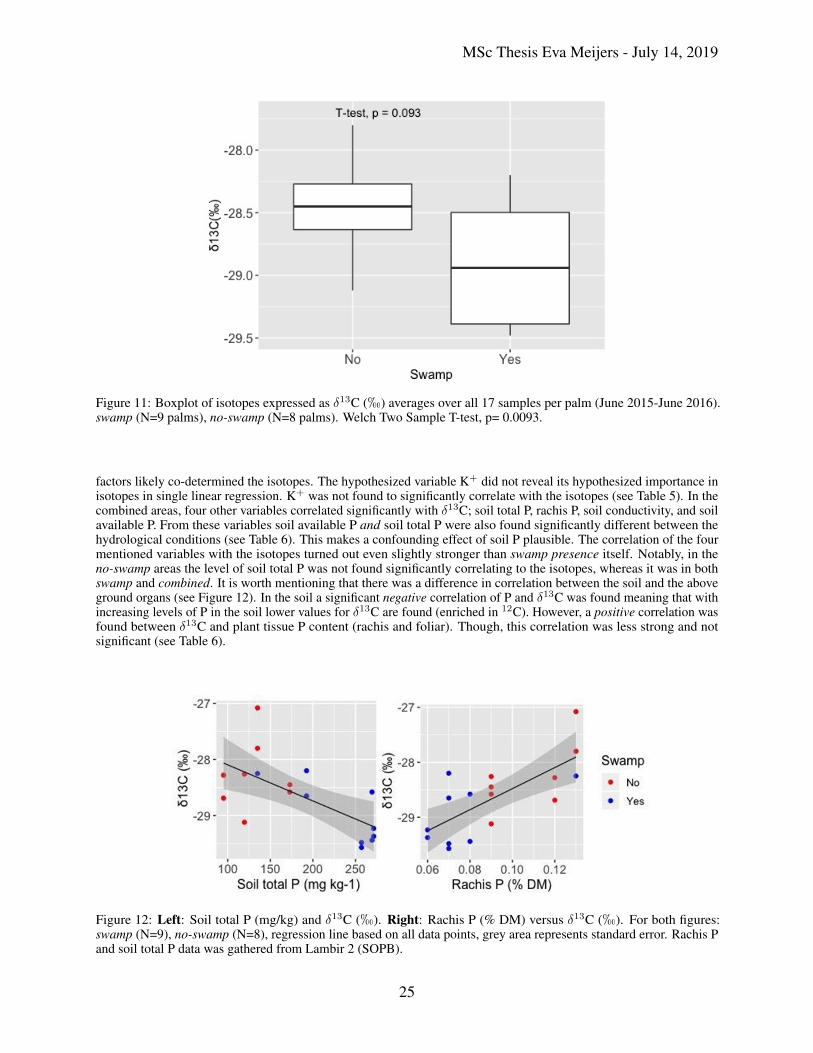
11 Boxplot of isotopes expressed as δ13C (h) averages over all 17 samples per palm (June 2015-June2016). swamp (N=9 palms), no-swamp (N=8 palms). Welch Two Sample T-test, p= 0.0093. . . . . . . 25
12 Left: Soil total P (mg/kg) and δ13C (h). Right: Rachis P (% DM) versus δ13C (h). For both figures:swamp (N=9), no-swamp (N=8), regression line based on all data points, grey area represents standarderror. Rachis P and soil total P data was gathered from Lambir 2 (SOPB). . . . . . . . . . . . . . . . 25
13 Time series of yield for swamp (blue), no-swamp (red) SOPB (Mg ha−1 month−1). swamp N=10,no-swamp N=24). Precipitation(mm) (dotted line). Vertical black lines indicate the full ENSO periodfrom which samples were taken (Jun 2015-Jun 2016). Correlation between yield for hydrologicalconditions was r=0.83(p<0.001) (Pearson’s test). . . . . . . . . . . . . . . . . . . . . . . . . . . . . 27
14 Left: Boxplot of Yield (Mg ha−1 year−1) averages (2014-2017) per block for both hydrological condi-tions: swamp (N=10 blocks) and no-swamp (N=24 blocks). Welch Two Sample T-test: (p<0.01(**)).Data from Lambir Estate 2 (SOPB). Right: Boxplot of Yield loss (% difference in yield 2016 comparedto 2015) averages per block for swamp (N=10 blocks) and no-swamp (N=24 blocks). Welch TwoSample t-test: (p<0.001 (***)). Data from Lambir Estate 2 (SOPB) . . . . . . . . . . . . . . . . . . . 28
7

MSc Thesis Eva Meijers - July 14, 2019
15 Topography Map Lambir Estate 2. SOPB . . . . . . . . . . . . . . . . . . . . . . . . . . . . . . . . 47
16 Swamp areas: Map Lambir Estate 2. SOPB . . . . . . . . . . . . . . . . . . . . . . . . . . . . . . . 47
17 Semi-detailed soil mail. Map Lambir Estate 2. SOPB . . . . . . . . . . . . . . . . . . . . . . . . . . 48
18 Palms on dry soils . . . . . . . . . . . . . . . . . . . . . . . . . . . . . . . . . . . . . . . . . . . . . 49
19 Swampy soils . . . . . . . . . . . . . . . . . . . . . . . . . . . . . . . . . . . . . . . . . . . . . . . 49
20 Samples (top left): Interior,(top right): exterior, (bottom left): shredded, (bottom right): wood dust aftergrinding. . . . . . . . . . . . . . . . . . . . . . . . . . . . . . . . . . . . . . . . . . . . . . . . . . . 52
21 Soil Exchangeable K+ (cmol kg−1) and K+ content rachis (% dry matter). Soil water conditions:Swamp (blue) (N=10), No swamp (red) (N=24). . . . . . . . . . . . . . . . . . . . . . . . . . . . . . 54
22 Yield loss(%) and Ratios of cations in the soil. Swamp (blue) (N=10), no-swamp (red) (N=24). Left:Soil Exchangeable Mg:K. Black line indicates Target; 1.2:1 Right: Soil Exchangeable Ca:Mg. Blackline indicates target; 5:1. Swamp areas is imbalanced . . . . . . . . . . . . . . . . . . . . . . . . . . 54
23 Boxplot of Soil Exchangeable Mg2+ (cmol kg−1) averages per block: Swamp (N=9), No-swamp (N=8).T-test: p-value=0.11. Not significant. . . . . . . . . . . . . . . . . . . . . . . . . . . . . . . . . . . . 55
24 Q-Q plots: Residual analysis from full models of carbon isotopes created based on p-value. Forwardselection developed models for combined hydrological conditions. Lm= linear model. . . . . . . . . . 56
25 Q-Q plots: Residual analysis from full models of yield loss created based on p-value. Forward selectiondeveloped models for combined hydrological conditions. Lm= linear model. . . . . . . . . . . . . . . 57
26 Left: Observed discrimination (h) and Ci /Ca ratios. For Ca = 410 ppm. Hydrological conditions:swamp = Blue (N=9), no-swamp = Red (N=8). Dashed line indicates the Ci/Ca lower boundary level(Eq. 1.6). Right: Observed discrimination (h) and Ci /Ca ratios. Ca of 340 ppm. Data for both C3
and C4 species (with and without leakage of CO2 from bundle sheets (phi)) are presented. Courtesy ofEvans et al. (1986). . . . . . . . . . . . . . . . . . . . . . . . . . . . . . . . . . . . . . . . . . . . . 57
27 Pearson’ r values of fitting a linear model with precipitation (lag -3 to 3) and δ13C. Individual R values(codes represent palms) and the chronology r values are shown. In bold significant correlations. In grey:correlations more negative than -0.5. Chosen applied lag times with best fit with chronologies indicatedby boxes with thick black lines. . . . . . . . . . . . . . . . . . . . . . . . . . . . . . . . . . . . . . . 59
28 Sampling elevation effect on δ13C (h). Not all elevations were recorded during sampling explainingthe presence of only 4 points for no-swamp. All no-swamp palms were located on top of hills oncomparable elevations as the one measured. . . . . . . . . . . . . . . . . . . . . . . . . . . . . . . . 60
29 Elevation effect on soil Mg(cmol (+) kg−1). Not all elevations were recorded during sampling explainingthe presence of only 4 points for no-swamp. All no-swamp palms were located on top of hills oncomparable elevations as the one measured. . . . . . . . . . . . . . . . . . . . . . . . . . . . . . . . 60
8

MSc Thesis Eva Meijers - July 14, 2019
1 Introduction
1.1 General
Anthropogenic global warming has resulted in increasingly extreme temperatures in tropical regions3. Predictions arethat CO2 levels will further rise, precipitation patterns will be disrupted even more, agricultural yields will becomeuncertain and droughts will further increase in both severity and frequency1,3,4. Droughts are infamous for disruptingagriculture and with that further complicating our ability to meet current and future food demands5–8.
Little is known of the underlying mechanisms via which agriculture is disrupted upon a drought complicating thepredictability of future productivity9–12. Moreover, knowledge is limited regarding potential mitigation of these negativedrought effects. Suggestions are made that proper nutrient management of especially potassium (K+) could alleviatedrought stress in plants13–18. However, the link between K+ and droughts in large-scale commodity crop productivityremains relatively unexplored.
This study focuses on drought responses of the highly important tropical commodity crop: oil palm (Elaeis guineensisJacq.). In this pilot study, a novel approach was tested to quantify the drought response using isotopes while assessingthe role of K+ herein.
1.2 Background
One way of studying and analysing drought responses is by means of stable isotopes12. The stable-isotope techniquemeasures the ratio of isotopes in a specific compound. Simply speaking, molecules can have multiple stable isotopeswith differing weights based on the number of neutrons, e.g. 12C versus 13C, where the number indicates the atomicweight. The stable-isotope technique is based on “fractionation of isotopes”. Fractionation is a process in which thecomposition of isotopes in a mixture (either gas, solid, liquid) becomes more divided, yielding a new ratio (heavyisotope/ light isotope, e.g.
13C12C . This isotopic ratio is then compared to an internationally recognized standard (V-
PBD19). Conventionally, this isotopic signature of samples is expressed in permille with a small delta notation (δ13C).Processes driving the fractionation are commonly expressed in permille by capital delta notation (∆). This ∆ sayssomething about the magnitude of the influence of the processes driving the fractionation, namely that fractionation canbe driven by various processes such as carbon uptake of plants or evaporation of water to air.
1.2.1 Carbon fractionation in plants
Fractionation of carbon is based on the fact that plants discriminate against heavier isotopes; in carbon, 13C is theheavier isotope compared to the lighter 12C (see Figure 1). Plants prefer to built the lighter isotopes into their tissues,though, not completely excluding the heavier isotope15,18. This translates into an isotopic ratio. With open stomata,there is a continuous flux (both in-and out) of CO2, H2O and O2 over the stomata (see Figure 1 left). However, wheneverstomata close, the internal CO2 (Ci) becomes scarce and no new influx of CO2 will take place (e.g. during a drought)(see Figure 1 right). Plants, then, increasingly start to build the heavier isotope into their tissue since they need to meetthe secondary assimilates requirements for internal maintenance. In the example of a drought, this results in an isotopicratio enriched in 13C, creating a larger isotopic ratio (>
13C12C ). The greater the impact on this isotopic ratio, the more the
plant was affected by the stressor, or in other words, “more fractionation of the carbon isotopes took place”. This largerisotopic ratio during the drought would then consequently exhibit high δ13C values (see bottom of Figure 1).
In more physiological detail, carbon fractionation takes place in multiple processes within plants. The "first" fractionationoccurs at the stomata as a result of the process diffusion20(see Figure 1). Namely, 13CO2 diffuses slower than the lighterisotope due to its heavier weight. Additionally, a ternary fractionation effect takes place which is the result of gascollision between H2O, CO2, and O2 when both in- and out fluxes occur simultaneously when stomata are open15. Then,fractionation occurs during diffusion of CO2 over the mesophyll cells towards the carboxylation sites (mesophyll =cells in the middle of the leaf). A fourth, fractionation takes place at the carboxylation reaction catalysed by the enzymeRuBisCO16,18,19. The heavier isotope 13CO2 causes a lower reaction constant here. Even further fractionations can takeplace downstream of RuBisCO (e.g. during assimilation of secondary assimilates or later lay down of compounds suchas tannins). Table 2 provides an overview of fractionations and other processes influencing isotopic signatures.
Measuring isotopes is generally used to assess the level of past stomatal conductance as RuBisCO usually functionsproperly when no nutrient deficiencies are at play21,22. However, alternative fractionations might cause noise in measuredisotopes data sampled from woody tissue. Isotopic signals can be distorted by factors such as: soil moisture23–27, lowhumidity28–30, irradiance31,32, temperature33,34, nitrogen availability35,36, salinity37–39, autotrophic versus heterotrophicmechanism14, atmospheric CO2 concentration40–42, and lastly sugar transport14,19,43.
9

MSc Thesis Eva Meijers - July 14, 2019
Figure 1: δ13C isotopic fractionation in two scenarios; Left: high humidity and low temperatures, Right: low humidityand high temperatures. Courtesy of Helle and Schleser (2004)
In more detail on sugar transport, it is known that primary sugars which are commonly used for sugar transport exhibita δ13C (compared to international standard) similar to those of the carbon initially fixed in photosynthesis. On the otherhand, downstream assimilates such as cellulose, lignin and tannins tend to reveal more negative numbers for δ13C14,19,43.When a "whole-wood" sample is analysed for its isotopic signature, downstream assimilates are measured as they arethe most abundant components in whole-wood. Whole-wood in dicotyledon species is known to be non-functional interms of productivity and/or transport of compounds. Nonetheless, the presence of primary sugars (also referred to asNon-Structural Carbohydrates (NSC)) in the sample might distort the signal18,20,43–45. These NSC are often used andtransported in- and between functional organs of the plant during times of stress and/or high sugar demand46. When asample is taken from a productive part of the plant (e.g. leaf) this NSC usage can be witnessed in the isotope ratios14.
Nonetheless, generally, isotopic signatures of "whole-wood" samples closely reflect stomatal conductance. For thisreason, isotopic signatures are commonly used in reconstructive paleo-climates as stomatal conductance can be used as aproxy for the level of precipitation18. This retrospective analysis of plant isotopes is currently used in many non-tropical
Table 2: Magnitude of fractionations and processes influencing isotopic signatures. ∆ represents the change in isotopiccomposition induced by the plant. References shown are the ones used in this study.
Symbol Fractionation ∆ (h) Reference
a diffusion through stomata 4 Francey & Farquhar,1982Craig, 1954
b carboxylation by RuBisCO 27-29 Francey & Farquhar,1982ab diffusion over boundary layer 2.8 Farquhar, 1983
Farquhar & Cernusak, 2012as diffusion over the stomata 4.4 Farquhar & Cernusak, 2012am dissolution & diffusion over intercellular spaces
to carboxylation location in chloroplast 1.8 Farquhar & Cernusak, 2012t ternary effect from gas collision 1.8 Cernusak, 2012e day respiration 1-5 Farquhar & Cernusak, 2012f photorespiration 8-16 Farquhar & Cernusak, 2012n.a. creating secondary assimilates:
cellulose 2 Lamade et al. 2009lignin unknowntannin unknown
10

MSc Thesis Eva Meijers - July 14, 2019
dicotyledon species with annual tree-rings13–17,43. Annual tree rings make it possible to sample a desired time frameof the past which then can be linked to a specific isotopic signature representing the level of stomatal conductance(and thus precipitation). However, the usage of annual rings still falls short on performance on both long term as wellas sub-annual resolution12. Moreover, the applicability of the technique is limited in the tropics as tree rings are notas distinctive in areas where the climate permits year-round growth compared to temperate zones. Though, tropicalisotopic studies are lately advancing. Various studies now show findings where tropical tree species show similarcorrelations between carbon isotope ratios and precipitation as temperate tree species (dicots)47.
Isotopic signatures can alternatively be used to assess plant responses to drought when climate data is readily available.The isotopic signatures then tell us something about the magnitude of the plants’ response in terms of stomatalconductance during a drought. Drought are known to have apparent isotopic signatures due to enforced stomatal closureleading to an internal shortage of CO2 which in turn lowers discrimination against the heavier isotope (13C)18,21,22.Hence, more positive ( +1-5h) ratios of δ13C are found in tissue created during a drought48. Unfortunately, the lack ofsub-annual resolution makes it complicated to assess the direct plant response to the drought (droughts usually lastshorter than a year). Coming back to the subject of this study, important commodity crops are often grown in the tropicse.g. oil palm, though increasingly suffering from droughts.
1.2.2 Oil palm and production
Oil palm (Elaeis guineensis Jacq.) is a monocotyledonous perennial crop characterized by simple architecture whichgrows in tropical climates49. It provides 30% of the world’s vegetable oil supply and is grown on 18 million ha50.Currently, the vast majority of palm oil production takes place in Malaysia and Indonesia, accounting for 85% of thetotal area under oil palm production51,52. The average productivity of oil palm is 3.5 tonnes ha−1 of oil53, which isalmost four-fold the production of other oil crops which illustrates the highly productive trait of the crop. The 3.5tonnes ha−1 is only one third of the estimated potential yield, leaving large room for improvement. The demand forvegetable oil simultaneously increases with 3.2% year−1 with the continuously increasing world population1,50. It isestimated that the demand for vegetable oil will reach a total of 240 Mt by 2050 of which 120 to 156 Mt will compriseof palm oil54. This would total an additional 20 million hectares of oil palm using current management or doubling ofproductivity in current oil palm plantations through intensification of management. With the latter having the preferencein order to avoid further deforestation of primary forest55.
1.2.3 Drought response in oil palm
Droughts hamper the potential of achieving the required increase in productivity in oil palm by reducing productionduring- and after the drought. For example, a major drought took place at the start of 2016 which resulted in adrastic drop in Crude Palm Oil production (CPO) of 13% in Malaysia1,53,56–58. This drought was the result of an ElNiño-Southern Oscillation event (from now on referred to as ENSO) (for more information on ENSO see58,59.
Oil palms require 200 mm month−1 of precipitation, though critical water deficit thresholds at different stages ofpalm development remain undefined53,60. In oil palm plantations precipitation is generally the only source of watereven though irrigation might be beneficial61. When precipitation levels drop below ±100 mm month−1, oil palmsstart to reveal severe stress responses of which the underlying mechanisms are currently still not understood60. Thestate-of-the-art states that oil palms are exceptionally sensitive to changing weather conditions. This is because oilpalms exhibit only minor phenotypic plasticity when induced by resource limitation or stressors49. Minor phenotypicplasticity means that the architecture and/or morphology of the plant does not substantially assist the plant during adrought by for example wilting. Oil palms do take alternative actions other than phenotypic plasticity to maintaininternal water status, however at a cost of productivity hence the witnessed production drops62. The primary responseof an oil palm to drought is stomatal closure induced by water withdrawal from the guard cells assisted by potassium63
(see Figure 2). This withdrawal from guard cells appears to especially occur in response to Vapour Pressure Deficits(VPD) and top soil humidity49,61,64. In turn, VPD and soil humidity are closely related to levels of water retention ofthe soil determined by factors such as soil organic matter and/or clay. Though, the exact underlying mechanisms remainrelatively unexplored.
Secondary drought responses in oil palm include an abortion of inflorescence, a change of the sex ratio of the flowerstowards more male flowers, reduced leaf area, slowed down growth in plantlets, usage of NSC reserves from the trunk,and a delay in leaf opening6,8,14,61,64–72. All these drought responses then in turn take place in different phases during adrought. Again, little is known of how these responses are induced or what the underlying mechanisms might be.
11

MSc Thesis Eva Meijers - July 14, 2019
Figure 2: Stomatal opening and closure. Courtesy of Lau (2017)
1.2.4 The role of potassium (K+) in drought responses
Potassium (K+) is known to be of paramount importance in drought tolerance in other perennial species13–17,17,18,43.Namely, lower net photosynthesis rates during droughts were found in K-deficient plants; examples of these speciesare: mung bean and cowpea73, faba bean74, wheat75,76, maize77, hibiscus13 and eucalyptus78. K+ might thereforebe involved in the still unknown mechanisms behind the above mentioned drought responses. K+ influences leafosmotic adjustments76,79, functions in protection against oxidative damage76,80, photosynthate loading into the phloemsap78,81,82, fruit production67, root growth83,84, stem elongation, disease resistance and enzyme activation67,76,77. Amore detailed description of the role of K+ can be found in Appendix 7.1.
In oil palm, a start was made to elucidate the role of K+ during droughts by Aslam et al.77; they found that K-deficientoil palms lack an acute sensitivity to water deficit. Moreover, preliminary research suggests that drought tolerance mightbe determined by the role of K+ in stomatal functioning85. However, no indisputable evidence came out confirmingthe effect at stomatal level in K+ deficient palms. Putrantro mentioned, though, that more extreme water shortageconditions are needed to amplify the response differences between K+ applications and hydrological conditions, forexample by using swamps versus no-swamps. If future research finds that K+ is beneficial to the plant during waterdeficit, there would be great opportunities to mitigate drought responses. This is especially valuable in tropical, peaty,sandy and acidic soils where K-deficiencies are common which coincide with land on which oil palm is cultivatedwhere additionally high prices for fertilizer exacerbate the deficiencies86. Literature states that there, K+ is usually thelargest nutritional factor that determines and correlates with yield67,77,78,87. The prevalence of K-deficiency in oil palmcultivated areas and the potential benefits during droughts from extra K application ask for further investigation on thesubject.
1.2.5 Studying drought responses in oil palm using isotopes from frond bases
Oil palms have a favourable physiology for isotope analysis in terms of their leaf production. Oil palms have oneapical meristem in a basin-like depression at the apex of the trunk88. The apical meristem is mostly a leaf producingmeristem. Spears originate from this apical meristem one by one and point vertically upwards. As the spear opens,the next one elongates to take its place. The leaves, called “fronds” in oil palms, are produced at a regular spatialpattern showing a phyllotaxis of 137.5◦. Fronds are simply pinnate comprising of the spine, petiole, rachis, leaflets withvestigial laminae and a terminal pair of ovate leaflets (see Figure 3). Oil palms carry between 32-48 open fronds66,89
which can grow from 10 cm up to 6 meter in 4-5 months14. Most importantly, oil palms produce fronds in a regular,approximate biweekly, pattern in their mature state (see Table ??). This fact makes it possible to determine when afrond was developed back in time and might be a suitable analogue for annual rings from dicotyledons. Part is leftbehind of these fronds after senescence or pruning. This is the frond base which connects to the trunk which previouslywas part of the petiole (see Figure 3). These frond bases adhere to the trunk until the palm is at least 12 years old, orsometimes even longer. Thus, theoretically, a time series of isotopes could be made of at least 12 years by sampling thefrond bases which are still connected to the trunk of the oil palm.
During a drought, the spear opening can be affected by water availability90; several spears may elongate before theoldest opens, creating a cluster of nearly fully elongated spears, though unopened53. This decrease in spear openingtakes place to minimize assimilate-demand and can lead to considerable lags of general plant development in the order
12

MSc Thesis Eva Meijers - July 14, 2019
Figure 3: Left: Anatomy of an oil palm frond. Retrieved on 08-03-19. From IDtools; Palm morphology. Right: An oilpalm tree trunk texture with abscised frond bases. Retrieved on 07-03-2019, From Visut Thepkunhanimit.
Table 3: Years After Planting (YAP) and frond opening in oil palmYAP Number of fronds opening year−1 Reference
1-2 40-45 Broekmans, 1957; Gerritsma and Soebagyo, 1999; Corley and Tinker, 20166 20-25 Broekmans, 1957; Gerritsma and Soebagyo, 1999; Corley and Tinker, 201612-14 20-25 Broekmans, 1957; Gerritsma and Soebagyo, 1999; Corley and Tinker, 201621 17-20 Broekmans, 1957; Rafii et al., 2013; Woittiez et al., 2017
of months to years6,49,89,91,92. When water returns after the drought, the majority of this cluster opens simultaneously ina flush88. Alternatively, spear opening can be slightly affected by planting density, cultivar2, and fruiting activity93.Nonetheless, the regular frond initiation (development of the spears regardless of spear opening) makes it possible todate frond bases back to a specific moment in time, making them a suitable analogue for tree rings. Using frond basesfor isotopic analysis would overcome the difficulties of both the sub-annual resolution sampling found in tree-ringanalysis and the indistinctive annual rings usually found in the tropics.
Caution needs to be taken during data interpretation of the isotopic signal of frond bases with regard to potentialinterference from the above-mentioned drought responses18,44,49. Contrary to dicotyledons, oil palms are monocotyle-dons where the woody tissue of the stem still takes part in the overall functioning of the plant. This means thatcompounds are actively transported through the whole stem and not just in the xylem and phloem vessels as occurs indicotyledons. As previously mentioned, primary sugars and starch exhibit different isotopic ratios compared to celluloseand lignin18,20,43–45. It remains unknown to what extent the proposed frond bases are subject to this NSC transport.However, frond bases are not expected to play a large role in the plants’ functioning after abscission.
Isotopic signatures from frond bases could provide useful insights in the role of K+ in droughts as isotopes generallyreflect stomatal conductance and K+ is expected to mediate this process. Yield numbers related to K+ levels are in thatsense less insightful as yields are the result of a large range and combination of factors.
1.2.6 Aim of this research
In this pilot study, the drought response of the tropical commodity crop oil palm is investigated using a carbon isotopeanalysis. A novel approach is proposed to overcome the current lack of sub-annual resolution and indistinctive annualrings by using physiological traits of the crop. The usability of frond bases for carbon isotopes analysis as an analoguefor annual tree rings will be tested by matching the time series with climate data. Herein, the isotopic signature of asevere drought will be sought and analysed in respect to K+ involvement. The results will hopefully provide moreinsights in the underlying mechanisms of oil palm drought responses. The results could be a step ahead in mitigationdrought driven production losses.
13

MSc Thesis Eva Meijers - July 14, 2019
1.2.7 Research questions
Part I: Detecting drought responses using carbon isotopes
The main research question is as follows: “Can carbon isotopes be used on frond bases of oil palms for analysis of theirdrought response?” The hypotheses here are four-fold:
1. Oil palm frond base tissue created after the onset of the most severe drought months of the ENSO will show apeak (±1-5h) in δ13C ratios.
2. A δ13C time series of frond base tissue will show a negative correlation with precipitation during the ENSO.3. Oil palms grown on dry soils will show higher values for δ13C compared to oil palms on wet soils.4. K+ will negatively correlate with carbon isotopes.
Part II: Yield loss and soil water analysis
Secondly, to elucidate oil palm drought responses, the following question was raised: “What are accurate predictors ofyield loss induced by a severe drought?” Hypotheses related to this question are:
1. The negative effect of ENSO on yields will be less severe on wet soils compared to dry soils.2. Plant K+ will be a strong negative predictor of yield loss during the ENSO on dry soils compared to wet soils.
3. Soil organic carbon will be a strong negative predictor of yield loss during the ENSO, especially on the drysoils.
4. Soil clay content will be a strong negative predictor of yield loss during the ENSO, especially on the dry soils.
14

MSc Thesis Eva Meijers - July 14, 2019
2 Methodology
2.1 Site description
Oil palm samples were taken during September 2018 from Lambir Estate 2 owned by Sarawak Oil Palms Berhad(SOPB) (N 4◦152.234, E 113◦ 966.021) in the area of Miri, Malaysia Sarawak (Borneo). The area is characterized by atropical climate with stable temperatures around 30◦C, with exposure to increasingly frequent droughts5. The estate islocated approximately 15 kilometers off the coast. The terrain contains both hilly slopes and valleys, both on mineralsoil (see Appendix 7.2 for edaphic condition), with elevation ranging between 0 and 170 m above sea level (Appendix7.2). Precipitation was measured in situ on a monthly basis with a local rain gauge. Mean annual precipitation for thisparticular area was 2650 mm per year for 2010-2018, excluding the ENSO year of 2016. Below, local precipitation isdepicted for both the average (blue) and the drought year 2016 (red) (see Figure 4).
Figure 4: Local precipitation (mm month−1) in Lambir Estate 2 (SOPB). Blue line represents average precipitationover 2010-2018 excluding the ENSO year 2016 (N=7). Grey area represents the standard deviation from the mean ofthe monthly values. Red line represents the year 2016
2.2 Experimental set-up
2.2.1 Hydrological conditions and block selection within Lambir Estate
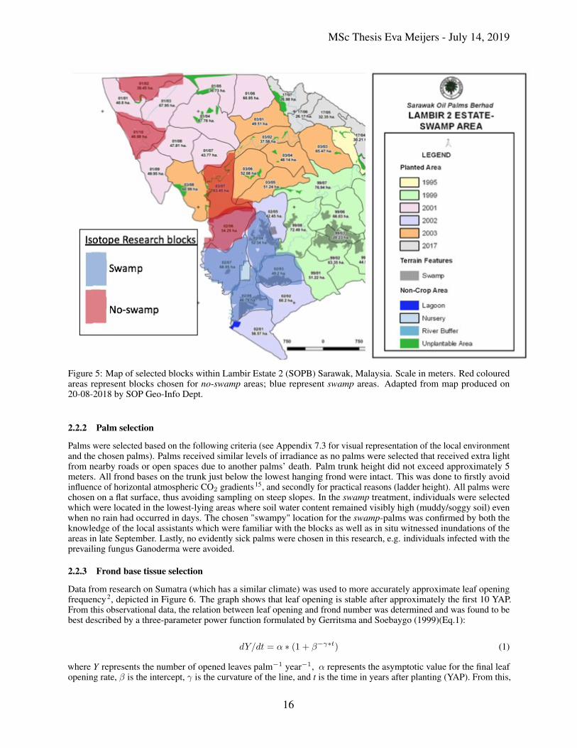
In this research two hydrological conditions were investigated; dry soils (from hereon referred to as no-swamp areas)and wet soils (swamp areas) (see Figure 5). Both hydrological conditions had 4 replicates (i.e. 4 blocks per conditionwithin the estate) with 2 palms per block to enhance statistical power and analyse the intra-block variation compared tointer-block variation. Hence, 8 blocks were analysed. In one block in the swamp areas, three palms were analysed tofurther enhance understanding of intra-specific variation in the isotopes.
From the data made available by SOPB, blocks were selected for homogenization to avoid confounding effects. Theblocks met the following criteria. All blocks were within an age range of 5 years to avoid palm developmental bias.Hence, all palms were approximately 10 years old during the ENSO year53. All palms were grown on a mineral soilat a density of 136 ha−1 with no managerial differences present between the blocks (e.g. the method of fertilizer ofapplication of fertilizer or the frequency). The selected blocks exhibited comparable values for the following parameters:clay content, pH, Cation Exchange Capacity (CEC), nutrient levels in the rachis and soil, soil organic carbon (SOC)content. Exceptions were made for the nutrient K+ which favourably differed between the blocks. The swamp blockswere selected based on the provided map (See black patches in Figure 5). Lastly, only blocks were selected with amininum 10% yield loss between the year 2015 and 2016.
15
MSc Thesis Eva Meijers - July 14, 2019
Figure 5: Map of selected blocks within Lambir Estate 2 (SOPB) Sarawak, Malaysia. Scale in meters. Red colouredareas represent blocks chosen for no-swamp areas; blue represent swamp areas. Adapted from map produced on20-08-2018 by SOP Geo-Info Dept.
2.2.2 Palm selection
Palms were selected based on the following criteria (see Appendix 7.3 for visual representation of the local environmentand the chosen palms). Palms received similar levels of irradiance as no palms were selected that received extra lightfrom nearby roads or open spaces due to another palms’ death. Palm trunk height did not exceed approximately 5meters. All frond bases on the trunk just below the lowest hanging frond were intact. This was done to firstly avoidinfluence of horizontal atmospheric CO2 gradients15, and secondly for practical reasons (ladder height). All palms werechosen on a flat surface, thus avoiding sampling on steep slopes. In the swamp treatment, individuals were selectedwhich were located in the lowest-lying areas where soil water content remained visibly high (muddy/soggy soil) evenwhen no rain had occurred in days. The chosen "swampy" location for the swamp-palms was confirmed by both theknowledge of the local assistants which were familiar with the blocks as well as in situ witnessed inundations of theareas in late September. Lastly, no evidently sick palms were chosen in this research, e.g. individuals infected with theprevailing fungus Ganoderma were avoided.
2.2.3 Frond base tissue selection
Data from research on Sumatra (which has a similar climate) was used to more accurately approximate leaf openingfrequency2, depicted in Figure 6. The graph shows that leaf opening is stable after approximately the first 10 YAP.From this observational data, the relation between leaf opening and frond number was determined and was found to bebest described by a three-parameter power function formulated by Gerritsma and Soebaygo (1999)(Eq.1):
dY/dt = α ∗ (1 + β−γ∗t) (1)
where Y represents the number of opened leaves palm−1 year−1, α represents the asymptotic value for the final leafopening rate, β is the intercept, γ is the curvature of the line, and t is the time in years after planting (YAP). From this,
16

MSc Thesis Eva Meijers - July 14, 2019
Figure 6: Leaf opening rates of oil palm of three cultivars (box, triangle, circle). The x-axis represents Years AfterPlanting (YAP). Dashed orange line represents the YAP from which the relationship was calculated to be close to linear.Adapted by Eva Meijers from Gerritsma and Soebagyo. (1999)
the integral was determined to calculate from when onwards the rate of leaf production would become stable. Thiscalculation was necessary to make it possible to use the fronds as an analogue for "tree-rings" to determine the frondnumber which coincides with the ENSO. The integral was as follows (Eq.2):
∫Y (t) = αt− αβ−γt
γlnβ+ constant (2)
Using the integral (Eq.2.), it was found that the relationship between YAP and total leaves became stable by approximat-ing linearity from year 6 onwards (see orange dashed line Figure 6). It was shown that 22 leaves year−1 are producedwhich corresponds to 1 leaf every 16.6 days. The authors stated that this rate is influenced by density and/or cultivar.The analysis of the determined density effect showed that this could only result in an error of ± 0.5 days; the cultivareffect only an error of ± 1 day2.
June 2015 was taken as benchmark as the start of the ENSO year time series so that the drought (Jan-March) would fallright in the middle of the time series. The frond number which corresponded to June 2015 was determined by dividingthe number of days that passed since the onset of the drought by the leaf production rate. A total of 1171 days hadpassed since then (start of sampling date in this study was August 15th, 2018). This number of days was then dividedby 16.6 days, which totalled 71 (i.e. the frond number of the start of the time series). A schematic representation of thesampled fronds from the oil palm crown is depicted in Figure 7, where the numbers represent the chronological orderof development (Courtesy of Lamade et al., 200914, adapted by Eva Meijers). The sampled fronds from the palmsare presented in either a red, yellow or blue color; indicating precipitation levels (drought, dry season, wet season,respectively). The numbers indicate the frond numbers which correspond to a date presented in the table on the right(see Figure 7). The time series starts on the 1st June 2015 and ends the 15th of May 2016. Within this period, a severedrought was aimed to be captured (red fronds Jan-March 2016). Margins at the end of the drought period were added totake both potential errors and/or delays in drought response into account. A total of 17 palms were sampled from whicheach palm 17 samples were taken. Samples were taken every subsequent frond base (monthly resolution) from June2015 until June 2016. The monthly resolution was chosen to make sure that the yearly oscillation between dry and wetseason could potentially be made visible as well as those seasons only last for 3-4 months. Additionally, the sampling
17

MSc Thesis Eva Meijers - July 14, 2019
resolution was increased between January 2016 and June 2016. This increase served to make sure that the magnitude ofthe effect of ENSO was captured in the data. This way it would be less likely to overlook the drought response in theisotope ratios.
Figure 7: Schematic representation of (left turning) oil palm crown showing sampling strategy including frond ranknumbers. Coloured circles indicate sampled fronds with concomitant precipitation levels and/or season; dry season(yellow), wet season (blue) or ENSO drought (red). Table shows the sampled frond number and corresponding date.Actual sampling done in August 2018 and September 2018. Negative frond numbers refer to unopened spears. Adaptedfrom Lamade et al. (2009)2
2.3 Plant measurements
Sampling took place in the morning and early afternoon during the months August and October in 2018. A photographwas taken from 8m distance to the trunk in order to visually capture the environment for later reference (see Appendix7.3). GPS coordinates were recorded for all palms. The direction of the spiral on the trunk was noted. The locationof the required frond bases on the trunk were determined using the phyllotaxis of oil palms14. The youngest frond(number 1) was determined first (as it is easy to spot) and used for selecting the required oil palm frond bases (Figure 7).Then, the trunk was cleared of other vegetation to avoid contamination of the samples. With a hole saw (Bosch), chiseland hammer, samples were collected from the frond bases which composed of hard fibrous uniform tissue. The sampleswere taken at least 3 cm from the abscission site, on either side of the middle axis of the frond base. This was doneto standardize sampling. The samples were shredded manually with a knife to attain smaller fibrous pieces suitablefor grinding and decrease the chances of the samples becoming mouldy. The strong woody outer layer (0.5 cm) ofthe leaf bases was removed to create a more homogeneous, easily grindable sample (see Appendix 7.4). The sampleswere oven-dried at 70 C◦ for 24 hours in the local laboratory of SOPB. The average weight of the dried samples fortransport by airplane from Malaysia to the Netherlands was ± 2g. The samples were ground and sieved to 1.0 mm sizeat Wageningen University using the Retsch MM301. Three milligrams of the total sample were put into tin cups of 4x6mm. These were then folded into compact spherical shapes and put in 96-well-trays for transport to the EnvironmentalStable Isotope Laboratory, University of Leicester, UK. The carbon isotope composition of the samples was determinedusing a Sercon 20-20 Stable isotope ratio monitoring mass spectrometer (from here on referred to as IRMS). Standardprotocol was followed for the carbon isotope assessment (for more information consult Rightek manual). A standardwas used as a laboratory reference compound composing of wheat flour. The isotopic ratio of this standard was assessedprior to the analysis in the lab. The standard was measured between every 9 samples in order to correct for any offset ofthe mass spectrometer. A detailed sampling protocol can be found in Appendix 7.4.
18

MSc Thesis Eva Meijers - July 14, 2019
2.4 Collection of soil- and plant nutrient data
The measurements of the soil parameters were taken in either 2013 or 2014 by SOPB. Data on the following soilnutrients were available: total N and P, available P/K/Na/Ca/Mg. Data on the following soil properties were available:pH, CEC, clay/silt/sand content, loss on ignition (organic matter), loss on evaporation, and soil organic carbon (SOC)content.
Measurements on plant nutrients were done on the rachis and foliage by SOPB. Data from rachis tissue was measuredin either February or March 2016 (i.e. during the drought). Measurements on foliar tissue were performed either atthe start of 2015 or in the months February or March 2016. The following nutrients contents were measured in bothrachis and foliage: N, P, K, Mg and Ca. Additionally, foliar and rachis ash (the quantity of inorganic salts) levels weredetermined.
2.5 Calculations on δ13C
The composition of the isotopes in the samples was expressed by the ratio (δ13C) of the heavier over the commonlighter isotope, relative to an internationally recognized standard; 0.0112372 derived from Pee Dee Belemnite rock(V-PDB19). Carbon isotope ratios are expressed in promille (h). Isotopic carbon composition (δ13C) was determinedas follows (Eq.3):
δ13C = (RsampleRstandard
− 1) ∗ 1000 (3)
where Rsample and Rstandard are the isotopic fractions (13C12C ) in the sample and standard, respectively.
The data accuracy was assessed prior to any further analysis. Both the precision of the measurements by the IRMS andthe homogeneity of the samples was assessed by comparison with acceptable literature ranges48. The credibility of thecarbon isotopes was assessed by comparison with other C3 plants and oil palms from literature11,14,47,94.
From the measured δ13C values, observed discrimination could be calculated. Carbon isotope discrimination (∆) differsfrom δ13C in that it describes only that change in isotopic composition induced by the plant, eliminating variation as aresult of the starting value of the atmospheric CO2 used for photosynthesis20. It was calculated as follows95:
∆ =δair − δplant1 + δplant
(4)
where ∆ is the observed discrimination (positive number), δair = -8h, δplant the measured δ13C values (negativebecause they are depleted of 13C compared to the fossil standard). From this, the ratio between internal CO2 andatmospheric CO2 (Ci/Ca) was calculated as follows95,96:
∆ = a+ (b− a)CiCa
(5)
This can be transformed to:
CiCa
=∆− ab− a
(6)
where a = -4.4 and represents the fractionation (h) due to diffusion in air, b = -27 represents the fractionation (h) byRuBisCO16,18,19.
2.6 Chronology building
In isotopic studies on dicotyledons with annual rings only reasonable time series are included into chronologies(averaging of multiple plants). Therefore, the same was done in this study as follows. All time series were firstcorrelated (Pearson Product-moment test) with one another irrespective of whether they were in a swamp or in ano-swamp area. Then, for building the two chronologies, positive correlations of the time series within the hydrologicalcondition (swamp or no-swamp) were assessed based on their correlation score. Correlations higher than 0.5 wereimmediately accepted for inclusion into its chronology when also significant (p<0.05) (the 0.5 threshold was based on
19

MSc Thesis Eva Meijers - July 14, 2019
Fichtler, Helle, Worbes47). Then, additional correlations were accepted when the time series correlated to the previouslyaccepted palms with p-values smaller than 0.05 while also with r values smaller than 0.5. The carbon isotopes of thefronds were averaged over the palms accepted for the two chronologies. Standard deviations were derived in the samemanner.
2.7 Data analysis
Two datasets were available: the database of all blocks (“All blocks”) and the database including only the blockswhere samples were taken (“Used blocks”). In both databases the hydrological conditions were present (Combined,no-swamp, swamp). Since the “Used blocks” were selected based on earlier mentioned requirements, the blocks weremore homogeneous than “All blocks”. This difference in homogeneity between the data-sets made the results form“Used blocks” less prone to interference from other variables causing noise in the data.
Intra-specific variability was tested by correlating all individual δ13C values with one another using the PearsonProduct-Moment correlation test. The magnitude of this correlation was compared within and between hydrologicalconditions to check for a confounding effect.
For visual assessment the measured isotopes were normalized by subtracting the mean of the palm from every singlefrond. To correlate precipitation to the isotopes, the time-step resolution was first made equal within the whole isotopetime series to avoid correlating "NAs". Here, the smallest time-step possible was preferred. To create the 16.6 daystime-step for the whole time series, the missing values were filled up by assuming an identical isotope value of thedirect previous measurement. This was a reasonable assumption because changes in isotopes values are likely gradualand not erratic for this time-step resolution (autocorrelation). Practically this meant that the isotopic value found for 1stOctober 2015 was duplicated into the missing value for 16.6th October 2015. The same was done for precipitation asonly monthly precipitation data was available. Again, the missing values were completed by duplication. Even thoughmonthly precipitation is the sum of rain of the whole month, this duplication method was chosen based on the fact thatplants respond to cumulative rain numbers as water is retained in the soil. Alternatively, the amount of precipitationcould have been divided into two. However, this method is prone to error since isotopes are then potentially linked toincorrect precipitation levels (e.g. all precipitation could have occurred in the last week of the month).
Diurnal effect of transport from- and to the frond bases was assessed by testing significant difference using a WelchTwo Sample T-test (unequal variances).
Precipitation and the isotope series (both individual and chronologies) were then fitted with a simple linear model andassessed using Pearson Product- moment test to both18. Then, lag times for errors in leaf initiation frequency wereapplied to precipitation to assess improvement in fit between the isotopes series and precipitation. The magnitude ofthese lag times was determined as follows. From the calculations on the leaf initiation frequency it seems possiblethat over time a cumulative error in frond frequency estimation became present2. The δ13C values of the createdchronologies might not be perfectly aligned with actual time because of this. Negative lag times of -1, -2 and -3 monthswere included based on the error ranges indicated by Gerritsma and Soebaygo2. Additionally, younger fronds are lessprone to errors than older fronds in estimating their development date. This error was assessed visually by checkingwhether the magnitude of the correlation and variance improved over time. To account for the fact that the effect ofprecipitation can only be seen weeks/months after its occurrence, positive lag times were implemented (+1, +2, +3months) as well.
Averages per palm were taken over all sample δ13C values, creating one mean δ13C value. This mean was then comparedbetween hydrological conditions. This could result in a bias as resolution was higher during the drought period than inthe rest of the year. Caution was therefore taken here during data interpretation dependent on the magnitude of theδ13C peaks. Differences between hydrological conditions in variables other than nutrients were analysed using eitherWilcoxon test (non-normal distribution) or Welch Two Sample T-test (unequal variances). Examples of these were:yield, yield loss, clay content, etc. Differences in nutrients (foliar/rachis/soil) between the hydrological conditions(swamp versus no-swamp) were assessed using Welch Two Sample T-test97.
The following was done for both δ13C and yield loss for both datasets (All blocks and Used blocks). An explorativestudy was performed to assess potential co-influencer candidates with precipitation for correlation with the δ13C andyield loss values. First, the δ13C and yield loss values of the combined hydrological conditions were fitted to all otheravailable variables using a linear model. Then, the same was done for the separate hydrological conditions in orderto get insight in potential different mechanisms at play. The ten strongest correlating factors were included in furtheranalysis and are presented in the result section.
One step further was taken in finding predictors for both δ13C and yield loss. To assess the presence of collinearity,all variables were correlated with one another (Pearson’s Product-moment test)97. The variables showing stronger
20

MSc Thesis Eva Meijers - July 14, 2019
correlations than R2= 0.60 were evaluated for logical collinearity based on theory (e.g. the fractions of sand/silt/clay arelikely to be collinear). When collinearity could be confirmed by theory, only one single variable was used in the models.Multiple linear regression was used to create a model that attempted to predict both δ13C and yield loss separately withcombinations of the available variables. Again, this was done for the combined hydrological conditions and the separateones. The dataset “All blocks” was used here because of the higher number of data points. Forward selection (using theSTEP function in R Studio) was used for building the prediction model, where inclusion of the variable was based onp-value <0.05. The residuals of the model were assessed checked for normality.
21

MSc Thesis Eva Meijers - July 14, 2019
3 Results
The results related to part I of the research aim will be presented first which attempt to answer the question: “Cancarbon isotopes for frond bases be used for analysing drought response in oil palm ?”. Then, in part II, results will bepresented on predictors of yield loss due to the drought of 2015-2016, with emphasis on K+.
3.1 Part I: Detecting drought responses using carbon isotopes
3.1.1 Intra-annual variation in isotopes
Prior to data analysis, the accuracy of the measured carbon isotopes was assessed; all δ13C values ranged between−27.10h and −30.87h. Precision of the IRMS was 0.1h and homogeneity within the bulky samples 0.03h.
The time series of all measured absolute δ13C data are presented for both hydrological conditions; swamp (blue lines)and no-swamp (red lines; see Figure 8). Increasingly negative values in δ13C reflect more discrimination against theheavier carbon isotope 13C. The figure shows that there is variations in the isotopes of the fronds over time (i.e. no flatlines). Variation around the mean over the full year within the swamp was 0.49h and within the no-swamp 0.28h.During the drought period, variation around the mean was never larger than 0.49h. Thus, no outstanding peaks werewitnessed within the expected response period (see black lines Figure 8). In other words, the data within the responseperiod showed no divergent behaviour compared to the rest of the year. Additionally, no clear difference was foundbetween the dry and wet season in the data. The time series did not clearly visually reveal similar patterns with oneanother. Significant correlations between individuals were generally low (and negative) for both hydrological conditions;never higher than 0.62 (see Appendix 7.11). Moreover, there was no difference in intra-specific correlations betweenwithin compared to between hydrological conditions.
A potential diurnal effect on the isotopes by daily trans-location of sugars from- and to the frond bases was assessedbetween sampling times (morning, afternoon, unrecorded) (see Figure 9). Here a significant effect was found between
Figure 8: (A) High-resolution δ13C (h) profile of swamp (blue; N=9) oil palm (B) High-resolution δ13C (h) profile ofno-swamp (red; N=8) oil palm. N represents number of palms. Palm code given in the legend. In both figures, timeseries lasts from Apr 2015-Aug 2016. Sampling resolution was 33.2 days from June 2015-Jan 2016 (monthly); 16.6days from Jan 2016- June 2016) (biweekly). Black vertical lines indicate the expected response period from the severedrought period (Jan 2016-May 2016). Black dots represent number of samples per palm.
22

MSc Thesis Eva Meijers - July 14, 2019
sampling time (p<0.001, Welch Two Sample T-test). Hence, sampling time might be one factor creating noise in thedata and explaining the absence of the peak and seasonality in the data.
Figure 9: Sampling time effect on δ13C (h). Afternoon (14:00-18:30) (N=156), Morning (10:00-14:00) (N=91),Unknown (time not recorded) (N=43). N represents the number of samples. p<0.001, Welch Two Sample T-test(unequal variances) tested on morning and afternoon sampling.
3.1.2 Isotopic response to drought and precipitation
Time series for both precipitation and δ13C of the chronologies are presented in Figure 10. The δ13C values werenormalized to make a visual comparison with precipitation more comprehensible. A total of three palms was acceptedinto the chronologies per hydrological condition (see Appendix 7.5). Chronologies were shifted according to the best fitwith precipitation.
The first attempt to fit the chronologies to precipitation was made by fitting a linear model without a lag time (seeTable 4, column Month=0). No significant correlation was found here. A second attempt was made by applying sixlag times (see Table 4 month=3 until month=-3). A slight improvement in fit was found here compared to month=0.The highest scores were used for testing the proposed method; maximum correlation between precipitation and thechronologies was r= -0.52 (p<0.05) and r= 0.43 (p<0.05) for swamp and no-swamp, respectively (see Table 4). In otherwords, a difference in lag time in fit with precipitation was present between the hydrological conditions. For analysis ofindividual palm fit to precipitation see Appendix 7.5.
The created chronologies showed a weak correlation with one another (r=0.17, p=0.42, ns). Both chronologies revealederratic variance over the time period, though without substantial peaks in δ13C during the expected response period (seeblack lines; Figure 10). Standard deviations within the determined response period were never more than 1h for bothhydrological conditions. Both chronologies did not show clear intra-annual patterns in which seasons could be easilydistinguished. Notably, precipitation did not show its usual pattern, namely an unexpected drop in precipitation waswitnessed between August 2015 and October 2015 whereas those months should have marked the start of the rainy
Table 4: Pearson’ r values of fitting a linear model with precipitation (applied lag times from -3 until +3 months) andδ13C of chronologies. In bold significant correlations. Highest correlations were used for testing the proposed method.
Hydrological Condition Applied Lag time (Months)
N 0 1 2 3 -1 -2 -3
Swamp 3 0.3 0.32 0.15 -0.52 0.41 0.51 0.31No-Swamp 3 -0.08 0.45 0.24 -0.1 0.09 0.43 0.06
23

MSc Thesis Eva Meijers - July 14, 2019
Figure 10: Time series of normalized δ13C (h) of chronologies for both hydrological conditions: swamp (blue line)(N=3) and no-swamp (red line) (N=3). Coloured areas represent one standard deviation from the mean. Dashed blackline represents the corresponding time series of precipitation (mm). Solid vertical black lines indicate the El Ninoperiod in which a response is expected of δ13C. Applied lag time to no-swamp chronology is 1 month and the swampchronology 3 months. swamp correlation with precipitation: r= -0.52 (p<0.05), no-swamp correlation with precipitation:r= 0.45 (p<0.05) (Pearson’s r). Precipitation data was gathered from Lambir 2 (SOPB) in September 2018.
season. Though, importantly, a prolonged unusual drop in precipitation was witnessed after November 2015 until April2016 representing the ENSO drought. Though, during this period no coherent isotope peaks were found, instead asimultaneous unexpected gradual drop in isotopes in the swamp areas can be seen suggesting improved performance.
3.1.3 Influence of hydrological condition on isotopic ratios
Aside from the missing peak and seasonality in the isotope time series, a difference in carbon isotopes was foundbetween the hydrological conditions. A mean of -29.02h was found for swamp; for no-swamp -28.43h (see Figure11). Means were statistically compared and found different from one another (p-value=0.0093) where the no-swampshowed significantly higher values for δ13C than swamp. Variance was additionally larger in the swamp areas.
Table 5: Top ten predictor variables of δ13C of data from Lambir 2 (SOPB). Ordered in accordance to decreasing RSquared value (here only r value shown). Three hydrological conditions are shown: Combined (N=17), no-swamp(N=8) and swamp (N=9). Significance was determined by fitting a linear model. Grey boxes indicate nutrient variables.Significance codes: <0.01 ‘**’, <0.05 ‘*’, <0.1 ‘.’. Data was gathered from Lambir 2 (SOPB).
Database Used blocks
Hydrological Conditon Combined (N=17) No-swamp (N=8) Swamp (N=9)Variable r Signif. Variable r Signif. Variable r Signif.
1 Soil P total -0.67 ** Rachis Ash -0.31 Soil P total -0.78 *2 Rachis P 0.56 * Rachis Mg:K 0.31 Planted ha 0.70 *3 Soil conductivity -0.55 * Rachis Mg 0.31 Average mature ha 0.70 *4 Soil P available -0.54 * SOC -0.30 Rachis N -0.60 .5 Swamp presence 0.49 * Rachis K -0.30 Soil Coarse Sand 0.59 .6 Foliar Mg -0.48 . Soil Mg:K -0.28 Soil Conductivity -0.577 Rachis N -0.47 . Yield loss -0.27 Rachis P 0.538 Yield loss 0.46 . Foliar K 0.27 Soil Na 0.499 Soil Coarse Sand 0.46 . Rachis Ca:Mg -0.27 Foliar age sampling -0.4610 Soil Ca -0.44 Rachis N 0.26 Foliar K -0.44
Single linear regression of the isotopes showed that swamp presence, as an explanatory variable, in the combined areasexplained only 24% of the found variance of the carbon isotopes (r= 0.49 (p<0.1) (see Table 5). Meaning that other
24
MSc Thesis Eva Meijers - July 14, 2019
Figure 11: Boxplot of isotopes expressed as δ13C (h) averages over all 17 samples per palm (June 2015-June 2016).swamp (N=9 palms), no-swamp (N=8 palms). Welch Two Sample T-test, p= 0.0093.
factors likely co-determined the isotopes. The hypothesized variable K+ did not reveal its hypothesized importance inisotopes in single linear regression. K+ was not found to significantly correlate with the isotopes (see Table 5). In thecombined areas, four other variables correlated significantly with δ13C; soil total P, rachis P, soil conductivity, and soilavailable P. From these variables soil available P and soil total P were also found significantly different between thehydrological conditions (see Table 6). This makes a confounding effect of soil P plausible. The correlation of the fourmentioned variables with the isotopes turned out even slightly stronger than swamp presence itself. Notably, in theno-swamp areas the level of soil total P was not found significantly correlating to the isotopes, whereas it was in bothswamp and combined. It is worth mentioning that there was a difference in correlation between the soil and the aboveground organs (see Figure 12). In the soil a significant negative correlation of P and δ13C was found meaning that withincreasing levels of P in the soil lower values for δ13C are found (enriched in 12C). However, a positive correlation wasfound between δ13C and plant tissue P content (rachis and foliar). Though, this correlation was less strong and notsignificant (see Table 6).
Figure 12: Left: Soil total P (mg/kg) and δ13C (h). Right: Rachis P (% DM) versus δ13C (h). For both figures:swamp (N=9), no-swamp (N=8), regression line based on all data points, grey area represents standard error. Rachis Pand soil total P data was gathered from Lambir 2 (SOPB).
25

MSc Thesis Eva Meijers - July 14, 2019
When the hydrological conditions were assessed separately with single linear regression, in the no-swamp areas noexplanatory variables were found that could significantly explain the variance of δ13C (see Table 5). Though, in theswamp areas, three variables were found that significantly explained substantial shares of the variance; soil total P,planted ha (block size) and average mature ha (r= -0.78, p<0.05; r=0.70, p<0.05; r= -0.70, p<0.05, respectively) (seeTable 5).
Absolute differences in nutrient content between the hydrological conditions were assessed to test the hydrologicalconditions for confounding variables determining the isotopes (see Table 6). The mean pH of the hydrological areasused for the isotope analysis was 6.3 and 4.5 for swamp and no-swamp, respectively. Six nutrients were found differentbetween the swamp and no-swamp areas; foliar N, foliar Ash, rachis K, rachis Ash, soil P and soil total P (p-value<0.05)(see numbers in bold in Table 6). Special attention should be paid here to the fact that the levels of rachis K+ weresignificantly different between the hydrological conditions, however never deficient (see Table 6). The reason for thisdifference in rachis K+ was investigated in relation to other soil cations and can be found in Appendix 7.6.
A further step was taken using multiple linear regression for predicting the isotopes values, however, this section wasdecided to exceed the purpose of the first research aim and can therefore be found in Appendix 7.7.
Table 6: Average nutrient content (N, P, K, Mg, Ca, Ash, Organic C, Na) in Foliar, Rachis and Soil. swamp (N=10blocks), no-swamp (N=24 blocks). Data on nutrient content was measured at different times for the respective organs.Significance was tested using Welch Two Sample t-test. In bold are significant results. Data gathered from Lambir 2(SOPB).
Source Hydrological condition N P K Mg Ca Ash% DM % DM % DM % DM % DM % DM
Foliar Swamp 2.56 0.16 0.93 0.23 0.57 7.62No-Swamp 2.45 0.16 1.00 0.23 0.57 6.92p-value 0.05 0.71 0.17 0.99 0.99 0.04
Rachis Swamp 0.33 0.08 1.32 0.09 0.22 4.01No-Swamp 0.35 0.1 1.55 0.08 0.23 4.57p-value 0.09 0.22 0.02 0.38 0.76 0.03
Source Hydrological condition Total N P K Mg Ca Na Total P Org. Cmg/kg cmol(+)/kg cmol(+)/kg cmol(+)/kg cmol(+)/kg cmol(+)/kg mg/kg %
Soil Swamp 0.1 14.06 0.15 0.48 3.07 0.05 261.96 0.81No-Swamp 0.09 4.92 0.13 0.31 1.84 0.06 162.51 0.69p-value 0.54 0.03 0.51 0.23 0.48 0.59 0.02 0.44
26

MSc Thesis Eva Meijers - July 14, 2019
3.2 Part II: Yield loss and hydrological conditions analysis
3.2.1 Yield response to precipitation
Moving on from the isotope analysis, the following section is concerned with the analysis of yield loss due to theENSO drought in 2015-2016. A time series is presented containing the monthly average yields of the two hydrologicalconditions (swamp= blue, no-swamp= red) and corresponding monthly precipitation (Figure 13). A distortion can beseen in the yearly yield oscillation from January 2016 onwards. The effect that ENSO had on yield was an extendedperiod of lower productivity than usual after the dry period (see length of dip in yields between 2016-2017 compared todip at the end of 2015). During this extended period, yields did not turn back to normal with a usual productivity peakaround 2.5 Mg ha−1 month−1. Yields in 2016 remained below 2 Mg ha−1 month−1. This date (Jan 2016) coincideswith the onset of the ENSO drought period. Precipitation levels during the most severe ENSO months (Jan-Mar 2016)dropped below 50 mm month−1, whereas oil palms require 200 mm month−1). The year 2016 had a cumulative annualprecipitation of 779 mm compared to an annual mean of 2629 mm (mean taken over 2010-2018 excluding ENSO year2016).
Figure 13: Time series of yield for swamp (blue), no-swamp (red) SOPB (Mg ha−1 month−1). swamp N=10, no-swampN=24). Precipitation(mm) (dotted line). Vertical black lines indicate the full ENSO period from which samples weretaken (Jun 2015-Jun 2016). Correlation between yield for hydrological conditions was r=0.83(p<0.001) (Pearson’s test).
3.2.2 Difference in yield response between hydrological conditions
The hydrological conditions showed generally similar numbers and patterns in yields over the whole time series. Thecorrelation between the two was found r=0.83 (p<0.001). Though, clear differences between the hydrological conditionsbecame visible from January 2016 onwards where the no-swamp areas seemed to suffer more from the drought than theswamp areas. Yields and yield losses were statically tested and confirmed; the no-swamp areas showed lower yieldsand greater yield losses (2016 compared to 2015) than the swamp areas (see Figure 14). The annual average yield inthe swamp areas was 24.2 Mg ha−1 year−1; in the no-swamp areas was 22.2 Mg ha−1 year−1. The no-swamp areasshowed an average yield loss of 24.55% compared to 17.8% in the swamp areas. In other words, the no-swamp areasshowed 6% more yield loss than the no-swamp areas. Furthermore, the minimum for yield in no-swamp was lower thanusually after a dry season whereas in swamp this was not the case (see Figure 13). Though, as earlier mentioned, theyields in both hydrological conditions did not return back to normal for at least the rest of the year 2016. Yields ofthe hydrological conditions only re-synchronized at the very end of 2016. The graph additionally shows that, everytime precipitation dropped below 100 mm month−1 the yields of the no-swamp areas were lower than the yields of
27

MSc Thesis Eva Meijers - July 14, 2019
Figure 14: Left: Boxplot of Yield (Mg ha−1 year−1) averages (2014-2017) per block for both hydrological conditions:swamp (N=10 blocks) and no-swamp (N=24 blocks). Welch Two Sample T-test: (p<0.01(**)). Data from Lambir Estate2 (SOPB). Right: Boxplot of Yield loss (% difference in yield 2016 compared to 2015) averages per block for swamp(N=10 blocks) and no-swamp (N=24 blocks). Welch Two Sample t-test: (p<0.001 (***)). Data from Lambir Estate 2(SOPB)
the swamp areas. No analysis was done on the erratic precipitation pattern nor the yields of 2017 as it surpassed thepurpose of this study.
3.2.3 Role of K+ during drought
The relationship of K+ with yield loss was assessed and is presented in Table 7. For comparison, both databases areshown: the full database (“All blocks”) and the database including only the blocks where samples were taken (“Usedblocks”). Combined hydrological conditions logically have in both databases the highest number for N making themthe most trustworthy.
Differences in correlations were found between yield losses and the locations of K+ (rachis, foliar and soil) (see Table7). Numbers for the relationship between rachis K+ and yield loss were generally positive. This would mean that moreyield was lost with increasing quantities of rachis K+. In foliar and soil, no such signal was found concerning the signof the correlation with yield loss between the hydrological conditions. Rachis K+ significantly explained yield loss inboth databases in the combined areas with an r=0.81 (p<0.05) and r=0.37(p<0.05). Hence, even when blocks werenot homogeneous a significant correlation between yield loss and rachis K+ was found. This correlation could notbe explained by collinearity between K+ and swampiness. This strong correlation was not the case for foliar nor soilK+. With regards to rachis K+, in the no-swamp areas in "Used blocks" showed a strong positive correlation of r=0.96(p<0.05). Though, no significant correlation was found in swamp areas between rachis K+ and yield loss. Hence, theeffect of the level of K+ in the no-swamp areas was more pronounced than in the swamp areas.
Table 7: Yield loss correlation (Pearson’s r) with K+: rachis, foliar and soil. Databases: Used blocks, All blocks.Distinction is made between hydrological conditions: combined, no-swamp, swamp. Significance indicated in bold(p-value<0.05). Data from Lambir Estate 2 (SOPB).
Database Used Blocks All Blocks
Hydrological condition Combined No-swamp Swamp Combined No-swamp SwampN=8 N=4 N=4 N=34 N=24 N=10
Rachis K 0.81 0.96 0.46 0.37 0.30 -0.27Foliar K 0.57 -0.51 -0.90 0.08 -0.07 0.02Soil K -0.68 -0.93 0.16 -0.13 -0.12 0.16
28

MSc Thesis Eva Meijers - July 14, 2019
The finding of positive numbers between yield loss and rachis K+ was analysed by verifying whether this could bedue to the indirect effect of K+ fertilization namely higher production rates due to K+ fertilization could in theorylead to higher yield numbers and thus simultaneous higher yield losses. Though, the correlation between yield and K+
was found r= -0.12 (p=0.49, ns)(see Appendix 7.13), thereby making the indirect fertilization effect unlikely. Othervariables were additionally assessed for potential collinearity with K+ from which rachis ash was found to be likelycollinear (see Appendix 7.13).
3.2.4 Other predictors of yield loss due to drought
From single linear regression it was found that in the "All blocks" database swamp presence was the strongest predictorof yield loss (r=0.50, p<0.05, combined hydrological areas). Other significant variables were rachis ash, soil Mg, yield2014, rachis K, soil Mg:K+ and rachis N. When the hydrological conditions were assessed separately, the level of soilMg2+ and pH showed significant in the no-swamp areas; in the swamp areas SOC and soil silt. In the "Used blocks",more variables were found to significantly correlate to yield loss (mind that N was lower here). The earlier mentionedrachis K+ showed to be the strongest predictor in the combined areas (even stronger than swamp presence though lesssignificant). In general, K+, regardless of the location, showed to be among the strongest correlations with yield loss,especially in no-swamp. Aside from K+, rachis ash, swamp presence, coarse sand, soil P total, silt, yield 2014, soilmg:k ratio and soil CEC showed significant correlations (order of correlation strength). Notably, N was only 8 here.The results from single linear regression are presented in the Appendix 7.8.
The results from building the predicting model of yield loss using multiple linear regression are shown in Table 8. Thefinal model for combined hydrological conditions included 5 variables; swamp presence, soil Mg2+, SOC, rachis ashand yield 2014. Herein, soil Mg and rachis ash were the most significant explanatory variables. The model was able tosignificantly explain 46% of the variance in yield loss. Residual plot can be found in Appendix 7.9.
Table 8: Variable Inclusion Final Model Multiple Linear Regression Yield loss. Forward selection method using thetop ten variables from Pearson’s r with yield loss per palm. Combined hydrological conditions (N=17). Contains:Probability, significance, p-value, Adj.R Squared. Significance codes: <0.01 ‘**’, <0.05 ‘*’, <0.1 ‘.’
Database Combined (N=34)
Variable Pr(>|t|) Signif. p-value Adj. R Squared
1 Swamp presence 0.21472 Soil Mg 0.017 *3 SOC 0.058 .4 Rachis ash 0.049 *5 Yield 2014 0.075 .
Full model 0.0004 0.46
29

MSc Thesis Eva Meijers - July 14, 2019
4 Discussion
4.1 Part I: Detecting drought responses using carbon isotopes
The main research question of this study was whether carbon isotope analysis on frond base tissue can be used foranalysing oil palms’ drought response. The potential of this proposed method was tested by creating a annual timeseries based on dating the fronds via their regular frond production. An annual time frame was chosen in whichboth seasonality and a severe drought were present. Additionally, two hydrological conditions were analysed whichsupposedly further aggravated the drought in the no-swamp areas compared to the swamp areas.
4.1.1 Intra-annual variation in isotopes
The found data fell within plausible ranges in respect of isotope levels of C3 plants, isotope levels for oil palmspecifically, and isotope levels to plants in comparable precipitation conditions11,14,18,47,94,98,99. In literature, C3 plantsexhibit levels of observed discrimination between 8 and 24 h11. In this study, observed discrimination levels (convertedisotope ratios) were found between 20 and 24h (see Figure 11 and Appendix 26). In other words, oil palms were foundat the higher end of C3 plants revealing higher levels of discrimination which fit to tropical plants (favourable weatherconditions drive discrimination). Though, the sampled year represented a drought year which in this sense could havelikewise resulted in lower levels of discrimination. Nonetheless, the comparable order of magnitude strengthened theresults of measured isotopes. The data of this study fell in a very close range with data on oil palms from North Sumatrain 2003/2004 with normal weather (precipitation 2800 mm year−1)14. Isotope measurements were done on frond rank-6 until 57 of rachis tissue. In their study, the measured isotopes remained stable from rank 20 onwards exhibitingratios between -29h and -30h; whereas in this study swamp -29.02h (st.dev 0.7) and no-swamp -28.43h (st.dev0.53) were found (slightly less negative likely due to the drought)(see Figure 8 and 11). Data from other evergreenspecies showed a variance of on average 0.44h (2975 mm year−1 in Sierra de Lema Venezuela (sp. T.amazonia)) andin areas with lower rain levels 0.22h(1560 mm year−1 Dorado-Tumeremo Venezuela; sp. T. amazonia)47. Again,these variances were in the same order of magnitude as in this study. The precision of the IRMS measurements and thehomogeneity found within the samples (one triplicate) lived up to the standards of isotope analysis set by Ehleringer48.
The intra-specific correlations of carbon isotopes time series among individuals and/or between hydrological conditionswere generally inconclusive with a maximum of r= 0.62 and a negative minimum of r= -0.52 (see Appendix 7.11).Though, in literature intra-specific correlations between r=0.42 and r=0.78 were found in similar climatic moisturezones47. The correlation of individuals between hydrological conditions were seemingly as low as within the areas,which again contrasted with findings in literature. Nonetheless, significant positive correlations of individual isotopeseries where found (r>0.5) among the hydrological conditions in this study which made it possible to create thechronologies. This does suggest that at least the chronology-palms experienced a similar external factor controllingcarbon isotope discrimination.
4.1.2 Isotopic response to drought and precipitation
Although general variation was found in the isotopes, the drought nor the precipitation pattern were clearly reflected inthe isotopes time series (see Figure 8). Namely, variation around the mean over the full year within the swamp was only0.49h and within the no-swamp 0.28h, whereas variation in the drought period was hypothesized to be in the order of1-5h48 as formulated in the research aim. Hence, hypothesis 1.1 was rejected. Secondly, correlations of the isotopetime series (either individual or chronology) with precipitation were found inconclusive; few significant correlationswere found. Moreover, the sign was not consistent within these significant correlations; both positive and negativewere found (see Figure 4). The hypothesis was here that correlations between the isotope time series and precipitationshould have been significant and negative in the order of r= -0.5047 since this is commonly found in other isotopestudies13–18,43. Hence, the results of this study were in disagreement with the formulated hypothesis 1.2.
The inconsistency with precipitation revealed a distortion of the isotope signal since it did not clearly respond toprecipitation. In this study, the simplified model of carbon fractionation was used created by Francey & Farquhar96
(see Methodology 2.5). This model omits fractionation components “below” simply diffusion through the stomata(indicated by letter a) and/or carboxylation by RuBisCO (letter b). In fact, downstream fractionations are completelydisregarded in this model. As earlier mentioned, this simplified model normally suffices for matching with climatedata, however this appeared not to be the case in this study. Expected is that the distorted signal found in this studyis due to these omitted downstream fractionations and/or less likely the "underlying components" of diffusion andcarboxylation16,18,19,43,96,100. Five main factors are suggested to have distorted the measured isotopes: NSC (Non-Structural Carbohydrates), alternative whole-wood components, timing of hardening frond bases, unstable Cair, anddecomposition & respiration. Moreover, potential limitations in study design could be attributed to chronology creation,
30

MSc Thesis Eva Meijers - July 14, 2019
application of lag times, precipitation data accuracy and frond dating. In 4.1.4. the causes of the isotopic signaldistortion will be discussed followed by 4.1.5. in which the limitations of the study design on the measured isotopesratios will be disputed.
4.1.3 Influence of hydrological conditions on isotope ratios
A significant difference was found between the hydrological conditions where the no-swamp areas showed overallreduced discrimination compared to the swamp areas. This confirms formulated hypothesis 1.3. This finding is in linewith theory where carbon fractionation is driven by soil moisture23–27. The level of significance of the difference here(r=0.49, p<0.01) is rather surprising as no exact levels of the soil water table were measured aside from the formulatedbinary system swamp versus no-swamp based on a provided map supported by the knowledge of the local assistants. Inother words, the binary system was sufficient in creating two different hydrological conditions where soil moisturecontent differences were apparent even though the swamp areas were not permanently inundated. The fact that asignificant difference was found between the conditions supports that oil palms respond sensitively to level of soilmoisture. This exceptional sensitivity to soil moisture was earlier confirmed in studies on stomatal conductance49,61,64,92.
Based on the available data, it can not be excluded whether exposure to turbulence exerted a confounding effect on theisotopes. Turbulence namely affects the thickness of the boundary layer and with that it affects the diffusion over thestomata (ab; Table 2)100. Thickness of the boundary layer is known to respond to wind speed. And although ENSOis not known to cause higher levels of wind speed and/or turbulence in the area, a difference in elevation betweenthe hydrological conditions might have resulted in this higher exposure to turbulence and with that, thinner boundarylayers20(see Appendix 7.12 for elevation and isotopes). Thinner boundary layers can boost transpiration rates of theleaves (E), which worsens the water shortage in the no-swamp areas. This would have in turn translated into increasedstomatal closure which matches with the findings that no-swamp areas exhibited less discrimination against 13C thanthe swamp areas. On the contrary, higher wind speeds are also known to cool down leaf temperatures, leading to lesstranspiration29. Because of these contradicting mechanisms at play, leaf temperatures and/or exposure to wind shouldbe assessed in future research to understand better what is driving fractionation or what causes noise in the isotope data.Turbulence does not explain why the isotope time series in general reveal a inconclusive pattern with precipitation.
4.1.4 Causes of isotopic signal distortion
Utilization of non-structural carbohydrates (NSC) Considerable research has recently reported that sugar flowscan interfere with δ13C ratios18,20,43–45. Especially the usage of stored sugars from reserves appears to lead to largemisinterpretation of the carbon isotope ratios because these “old” assimilates would create a divergent carbon signature(namely one of the past) than what is expected. In oil palm, up to 20% of the total dry biomass was found to benon-structural carbohydrates which theoretically could sustain growth for 7.2 months46. Of these 20%, 13% resides inthe "persistent leaf bases" (i.o.w. frond bases)46. However, little is known of the rate of this usage. It could well be thatin the first weeks during stress, palms would use up considerable amounts of NSC upon which they enter a “hibernationmode” if the stressor remains too long. Details concerning this NSC usage remain unknown and should be addressedin future research although forcing a long-term stressor on a palm for NSC analysis in situ is extremely complicated.Utilization of storage reserves during a drought would create strong autocorrelation between isotopes (or correlation tofrond parameters from the climate in previous years)101 and limit the potential to directly reconstruct climates45,102.In this study, the assessement of the level of autocorrelation is unfortunately rather unreliable as only one year wassampled for the analysis. Nonetheless, from preliminary assessment of the months prior to January 2016, it seemsthat palms were not affected by any severe stressor (although no-swamp might be considered under stress comparedto research on North-Sumatra14) and are therefore the palms are expected to have some reserves. Then, during thedrought response period (Jan-April), no divergent behaviour compared to the previous months was found in the isotopes.This supports the idea of autocorrelation. In case "old assimilates" would be used for maintenance and growth duringa drought, they would reflect the same isotopic signature as prior to the drought. This could counter the anticipateddrought signal. Alternatively, relocation of “old assimilates” to other processes than frond growth/maintenance couldalso have taken place during the drought78,81–84. Namely, sugars could have been relocated for the purpose of rootformation to percolate deeper into the soil in search of water. Though, maintenance costs of the highly productivefronds are likely given priority during droughts over “extra” root growth. Moreover, sugars are likely first extractedfrom the stem and/or non-functional frond bases before extraction from the high maintenance fronds. This study did notsupport this theory of relocating of assimilates from the fronds elsewhere as it would have left behind an NSC (verynegative δ13C) depleted rachis during the drought, which should have corresponded to even amplified less negativeδ13C signature, which was not found in this study.
Alternative whole-wood components Downstream assimilation fractionations might have caused partial decouplingbetween “plant organ” and “wood/cellulose” carbon isotopes signals43. This means that the measurements might not
31

MSc Thesis Eva Meijers - July 14, 2019
represent the desired component of the whole-wood. In dicotyledons, whole-wood samples mostly contain cellulose andlignin, with little primary sugars present. These components have their own isotope signature as a result of downstreamassimilation fractionations (see Table 2). Downstream assimilation fractionations are the basis for the statement ofvarious authors that only α-cellulose should be used for long-term analysis48. However, other studies reported thatthe usage of whole-wood leads to little to no differences in the variability of the carbon isotope signal and thus shouldhave sufficed for the purpose of this research18,47,103,104. However, since the isotopic signal in this study was distortedin terms of lack of drought signal, the analysis of the abundance of these components might have helped explainingthe signal. Especially because the wood components are different between dicotyledons and monocotyledons (e.g.oil palms) as the wood still takes part in the functioning of the plant (notably old frond bases less involved then thestem). As no measurements were taken in situ on the composition of the frond bases, literature was used as a reference.A paper related to the pulp and paper industries quantified the chemical composition of oil palm fronds sampled inPerak Malaysia105. There, frond strands were rich in holo-cellulose (82.2%) and α-cellulose (47.6%). Lignin contentwas 15.2% which is slightly lower than normally found in hardwood (18.1% in aspen). Hence, no direct evidencewas found for these alternative whole-wood components based on this paper, making this route unlikely though notimmediately rejected. Measurements in this study were in the range of -29h, which is assumed to be the range of thedesired permanent downstream assimilates (cellulose and lignin). The influence of diurnal primary sugar transport from-and to the fronds on the composition of the fronds was rejected by testing whether there was a difference in isotopesbetween the morning and afternoon sampling time (see Figure 9). Hence, the statement that isotope measurements needto be taken at the end of the day because leaf starch and sugar contents are then at their peak concentrations48, did nothold in this study for the frond bases (only fronds older than 48 were measured). Nonetheless, in future research usingbulky whole-wood samples of monocotyledons, it might be valuable to quantify the contents (cellulose, tannins, etc.) ofthe samples at least once in triplicate to get a rough idea on the subject.
Timing of hardening of frond bases During a drought, oil palms are known to slow down their frond unfolding (notthe initiation of the frond). It can be argued that this leaf unfolding goes hand in hand with simultaneous hardening of thetissue since hardening is mostly necessary to provide stability to the frond. Hardening of tissue encompasses productionof secondary assimilates such as cellulose and/or lignin (the measured components of the samples). And as earliermentioned, these assimilates reflect a differing carbon isotope signal than primary assimilates. In case this hardeningof the frond bases was delayed during the drought, the samples could have reflected the isotopes of the moment afterthe drought when hardening and unfolding then again was resumed. This is in line with the found measurements asno peak was witnessed in the drought period. However as a counter-argument, caution was taken during sampling byremoving the hard outer layer of the frond bases which mostly provide the stability (see Appendix 7.4), which shouldhave resolved the issue. From Lamade et al.14, it is known that a younger frond bases from spears reveal a more positiveisotopic signature which was attributed to the difference of autotrophy and heterotrophy. However, this more positivesignature might have also been due to the hardening/lignification of the tissue as an overlooked confounding variable.In any case, to make any convincing statement on whether this influenced the data in this study, isotopes of the frondsshould be analysed from being a spear to becoming a remnant frond base during a drought and a non-drought.
Unstable Cair The Cair could have been influenced by amount of exhaust from the mill close-by which releasesplant-derived carbon into the atmosphere. Important here is that the burned material originally was plant materialwhich is known to have a divergent carbon signature than atmospheric CO2 (with the latter more positive). In thissense, capturing Cair derived from previously burned plant material could lead to high levels of autocorrelation andcancelling out of peaks & dents. However, as stated by Cernusak20, the atmosphere is generally well mixed and unstableCair levels occur only in very closed canopy forests, glasshouses and other situations where turbulent exchange of airbetween the plant canopy and the free troposphere is impeded20. Moreover, in case these exhausts would have had aneffect on the isotopes, then still a relative effect should have been visible in the isotope time series. An influence offorest fires on the Cair resulting from the ENSO drought was briefly examined by using the knowledge of the localassistant and newspaper articles. Here, a fire event was mentioned occurring on the 21 of February 2016 in NorthernSarawak. However, no effect was witnessed from this forest fire in the measured isotopes as no clear dent in the isotopeseries were quantified (see figure 10). Hence, influence by unstable Cair is assumed to be very unlikely, though cannotfully be rejected.
Local decomposition & respiration Alternative biological reasons behind the unstable level of Cair could havebeen local decomposition- and local respiration rates of microbes and plants48. It is known that CO2 concentrationscould namely increase as much as 100 ppm because of these factors. However, no measurements were available onthe matter. And, as earlier mentioned, the atmosphere is generally well mixed20. Nonetheless, assuming there was adifference between these local rates, swamp areas would then likely have lower rates than the no-swamp areas sinceinundation hampers these rates. This could have translated into less available Cair in the swamp areas leading to lessnegative numbers for the isotopes. This is in disagreement with the findings of this study. However, notably, this line of
32

MSc Thesis Eva Meijers - July 14, 2019
thought could explain the positive correlation between precipitation and isotopes in the no-swamp areas; with moreprecipitation less decomposition/respiration takes place leading to less discrimination and thus less negative isotopevalues. Recurring drying and wetting events are known to influence these decomposition- and respiration rates however,literature search on the matter exceeded the purpose of this study. Though, these rates might be extremely valuable infuture research as oil palm is often grown on peat soil (high water content) and should not be overlooked.
4.1.5 Limitations of study design on isotope measurements
Using the chronologies instead of all palms for assessment of the match with precipitation can arguably lead toinaccurate interpretation of the results. Namely, when few time series of individuals are included into chronologies,errors become more likely and standard deviations larger. In this study, only three time series were included in eitherhydrological condition chronology which is regarded as very few. Though, creating chronologies by excluding "noisy"time series and applying lag times is commonly done for fitting with climate data since it reduces the noise. And,considering this is a pilot study wherein the usability of carbon analysis was tested for detecting droughts, it was chosento include only strong significantly correlating time series for the analysis rather than noisy ones to hopefully filterout the precipitation effect. And since the swamp chronology did behave in the same order of magnitude as in otherpapers (r= -0.52, p<0.05) (although missing the anticipated peak in response to drought), overall systematic errors dueto chronology making are expected to be unlikely. Analysis of individual palm fit with precipitation also did not reveala better fit than the chronologies (see Appendix 7.11). Hence, the significant positive correlations found between theno-swamp chronology and precipitation (r=0.45, p<0.05) remains unresolved (see Figure 10).
Application of lag times might lead to inaccurate matching of the time series, especially when sample size is low. FromTable 4 it can be seen that applying lag time of 3 months results in a fit close to equally strong and significant to lagtime -2 months in swamp areas. For the no-swamp areas this was also witnessed where lag time +1 month and lag time-2 months were equal in strength. In both cases, the strongest correlation was chosen. Meaning that chances of bothdata misinterpretation with regard to matching with precipitation was present as well as bias by the choices that hadto be made for creating both the chronology with lag time. Interestingly though, this difference between the foundlag times can be supported by the idea that the swamp areas only revealed a response to drought 3 months after theonset of the drought whereas the no-swamp areas already 1 month after the onset. This might be due to the fact that theswamp areas only started to reveal effects of water shortage after their soil water reservoir was depleted whereas in theno-swamp areas the extend of their soil water reservoir was much smaller, hence the faster response. Further research isneeded to substantiate this idea.
The precision and accuracy of the precipitation data might have limited the performance of this study as it was thesingle factor representing the "drought climate". The accuracy of precipitation measurements was first assessed insitu by inspecting the local rain gauge where no signs of malfunctioning were found. Then, precipitation data wasassessed by distinguishing seasonal patterns and the drought within the data which were confirmed valid. The rainpattern clearly showed the onset of the severe drought at the start of 2016 (see Figure 4). Though it is worth mentioningthat the levels of precipitation were generally low for the whole area over the years (± 120 mm month−1), if not closeto deficient. This in turn might explain the found significant difference in isotopes between the hydrological conditionsas the no-swamp areas might have suffered from the drought even more than expected. In case of the general lackof precipitation in the area could be due to inaccurate measurements by the rain gauge, it still should not have madea difference in correlation to δ13C as only the relative patterns were assessed. Unfortunately, no suitable weatherstation was found in close proximity that could have validated the numbers (close proximity was necessary of 50km asprecipitation is spatially divergent).
Using an constant estimate of frond intuition of 16.6 days frond−1 for dating the fronds might have limited theperformance of the match between precipitation and the isotopes as it prone to error. This frond dating estimate accuracywas assessed using the knowledge that various authors state that droughts can be clearly visible in time series as theyhave an apparent isotopic signature18,21,22. Hence, in case the estimate for dating the fronds would be completely off orwhen the estimated would be different between individuals, this drought signature could have been used to align thetime series. Prior to the sampling, margins were built in by extra sampling at the end of the time series to avoid missingthe hypothesized drought period in the isotopes due to either mis-estimation of the frond development and/or delayof drought response (NSC usage). Unfortunately, still no drought signature was found, complicating the validationof the frond dating. The accuracy of the dating the frond bases was then alternatively visually assessed by testingwhether the fit between the isotope series would improve over time (errors sum up over time). In the case that thefrequency of 16.6 days frond−1 was too little or too much2, though constant, the seasonality pattern should have stillbeen visible. Though, no such improved fit over time nor seasonality pattern was witnessed. Since the study designwas so that the planting density, cultivar, fruiting activity was homogeneous between all fronds, no theory supports theidea that the rate of frond development was different between individuals within a hydrological conditions2,93. Thewater availability which is known to affect frond opening90 was taken into account by seperating the analysis of both
33

MSc Thesis Eva Meijers - July 14, 2019
hydrological conditions to avoid errors. Nonetheless, in any case, caution needs to be taken in interpreting the estimateddate of the fronds since assumptions can not be avoided regarding this subject.
4.1.6 Involvement of K+ during drought
K+ was hypothesized to play a large role during a drought by mediating stomatal conductance which was anticipated tobe reflected by high correlations between isotopes and K+ levels. This hypothesis was rejected based on the outcome ofsingle linear regression on data of this study. The differences in K+ in the data between the hydrological conditionsdid not reveal a clear pattern in δ13C values (no-swamp areas r= -0.30 (p>0.05, ns.) N=8), swamp r= -0.07(p>0.05,ns.)(N=9)). Here, it should be menetioned that K+ difference were only minor and isotopes did not seem to reflectstomatal conductance due to interference in the isotope signal. Hence, little can be stated on the involvement of K+
in stomatal conductance. It is worth mentioning that no K+-deficient palms were present in this research (difficult tofind in large scale oil plantations); though swamp areas had significantly lower levels of K+ with 1.32% DM rachisversus no-swamp 1.55 % DM rachis (p=0.02; see Table 6). Additionally, the effect of K+ might have been overruledby other factors as well such as soil hydrological conditions. More severe K+ differences between groups couldclarify relationships. Unfortunately, no time series of K+ levels on monthly resolution were available to fit with δ13C(only yearly data) which would have made the analysis of K+ and stomatal conductance more reliable and insightful.Therefore, in future research on the influence of K+ in stomatal conductance using isotopes, it would be valuable togather more data points of corresponding δ13C and K+ levels.
4.1.7 Involvement of P during drought
From the regression analysis, level of phosphorus (P) unexpectedly came out as strong explanatory variable with theisotopes (r=-0.67, p <0.05) (see Table 5). From literature analysis it was found that this P involvement could be relatedto stomatal density which is positively affected by the plants P levels106–108. And increased stomatal density in turnincreases stomatal conductance leading to more negative isotope values. Namely, enhanced discrimination would takeplace as more preferable carbon isotopes are available as a result of higher influx. In this study, this negative relationshipbetween P levels and isotopes was confirmed for the level of soil total P (mg kg−1), however, opposed by a positiverelationship between plant tissue P content (mg kg−1). However, plant (foliar or rachis) are more indicative for theeffect of P on stomatal conductance as they are present at the location itself. It is suggested that swamp presence hasa confounding effect on the level of soil total P rather than P having a forcing effect on δ13C itself. Namely, P is arelatively inert molecule and can only be taken up when accessible by the roots (not by dissolving in water like nitrate).Phosphorus uptake is especially driven by pH level where pH > 6 is known to go hand in hand with high levels of Puptake; when pH < 6 P is usually bound to aluminum or iron (e.g. Fe3+ or Al3+). And the no-swamp areas had a meanpH of 4.5, the swamp areas 6.3109. Hence, it was unexpected that the plant P levels did not follow this theory. Though,further analysis on the effect of pH and potential dilution via water exceeded the set time of this MSc thesis. Collinearitywas impossible to assess between soil P and swamp presence was only a categorical factor. Also, caution should betaken when interpreting the influences of the nutrients as those measurements were not done on the exact same locationand time as the measurements of the isotopes. In any case, the positive relationship between plant P and isotopes couldnot be explained by theory. Further research on P and δ13C might elucidate the unexplained correlations.
4.2 Part II Yield loss and hydrological condition analysis
4.2.1 Yield response to precipitation
The area receives relatively little precipitation in general; with an yearly average of 2650 mm compared to what iscommonly found in Malaysia and Indonesia (1700-4000 mm year−1 53,64,110. Therefore, the level of swampiness maynot have been as extreme in the swamp areas as initially intended. This was also supported by the visual healthyappearance of the palms in situ (see 7.3). Nonetheless, the precipitation data revealed the severe drop of ENSO resultingin an cumulative annual of 779 mm compared to the usual mean 2629 mm year−1. Plants mostly responded to thedrought by an extended period of lower yield (close to a full year) when compared to other dry periods (3-5 months)(see Figure 13). This suggests that more severe drought responses occurred than simply halting the growth of buncheswhich could have been resumed rather quickly after the drought. Examples of alternative severe drought responses arethe change of the sex ratio of the inflorescence towards more male flowers or a general decrease in flower development,however, no data was available on the matter. Whatever the exact mechanism was, the ENSO was clearly visible in theyield of both time series. The fact that the yields did not exactly follow precipitation levels is not surprising as yieldresponds to many factors, even though in literature a linear relationship was found between applied water volume andyield in drier environments53,89,111. It is worth mentioning that in this study no investigation was done on the effect ofhaze due to lack of data although haze is known to hamper yields, especially during droughts when haze is a common
34

MSc Thesis Eva Meijers - July 14, 2019
phenomena6. Analysis of this haze effect simultaneous with the water-shortage effect could be therefore valuable infuture research.
4.2.2 Difference in yield response between hydrological conditions
The strong level of correlation in yield the hydrological areas (r=0.83, p<0.0001; see Figure 13) suggested that therewas no general water shortage in the no-swamp areas as yields were comparable (contradicted by isotope data),especially when precipitation levels were above 150 mm month−1. Arguably, the similar performance between thehydrological conditions are in itself surprising as oxygen stress by temporal submergence could be anticipated in theswamp areas. This oxygen stress at the roots could have resulted in coherent lower yields regardless of their abilityto form pneumatodes53,88,112. Though this lower yield due to waterlogging was not supported in this study. Though,the fact that the area receives relatively little precipitation might have counter-acted this effect. The strong generalcorrelation in yields between the hydrological areas could have also been due to general over-performance of theno-swamp areas. For example, a bias towards better soil structure or fertility in the no-swamp areas might have elevatedthe water holding capacity of the soil in these areas when precipitation was > 150 mm month−1. However, such abias was not found. For example, SOC nor clay content were systematically higher in the no-swamp areas (see Table6). Even though it was not mentioned by the local employees, it can not be excluded that slightly more efficientmanagement (harvesting, pruning, fertilizing, culling, weeding) in the no-swamp areas took place as they are moreaccessible which in turn could have resulted in found higher yields53.
Although the yield patterns of both hydrological conditions correlated strongly with one another, a difference becamevisible when precipitation levels dropped below 100 mm month−1. This precipitation threshold of 100 mm month−1
is in agreement with literature59,60. In this study, the no-swamp areas revealed in general a more severe drop in yieldcompared to the swamp areas upon limited precipitation. Quantification of the yield losses due to the ENSO drought(2016 compared to 2015) showed that the no-swamp areas indeed exhibited an average of 24.55% yield loss comparedto 17.8% in the swamp areas. Hence, hypothesis 2.1 was confirmed where the no-swamp significantly exhibited 6%more yield loss than the swamp areas (see Figure 11). Notably, this difference could not be attributed to general lowerperformance as mentioned earlier. In fact, the likelihood of having more apt management of the blocks in the no-swampareas suggests that the measurement differences in yield losses might even have been a underestimation. In any case,the difference in yield losses lays predominately in that the no-swamp areas show more severe yield reduction than theswamp areas.
4.2.3 Role of K+ during drought
The level of plant K+ was hypothesized to be negatively correlated to yield loss based on the theory that K+ is beneficialto the plant during a drought. In this study positively correlating numbers were found between yield loss and K+. Hencehypothesis 2.2 was rejected. It is worth mentioning here that this rejection of the hypothesis is based on the rachis K+
numbers; not on the foliar and/or soil K+ levels. This usuage of rachis K+ is in accordance with literature as rachistissue is known to correlate strongly with the plant’s K status and yields53,77,78,87,113–115, which was also supported bythe findings of this study (see Table 7). Though, the likelihood of K+ having a negative effect via stomatal conductanceon yield during droughts is arguably low. Namely, K+ is expected to fine tune stomatal closure and aperture, not forceaperture.
The counter-intuitive findings of K+ were therefore investigated and tested on a potential fertilization effect via yield,which in turn could have led to higher yield losses. However, this was not found. Secondly, the effect of coincidencewas analysed by taking into account the larger database "All blocks" instead of the "Used blocks". Again, coincidencedid not seem to cause the odd finding: the strength of the correlation of K+ with yield loss did decrease here fromr=0.81 (p<0.05) to r=0.37 (p<0.05), though remained significant, strong, and positive. Correlation of rachis K+ wasassessed where no conclusive variables revealed importance other than rachis ash (see Appendix 7.13). No literaturewas found confirming the collinearity between the two variables nor suggesting potential routes to support the finding.All in all, the abundant presence of K+ in all forms in the top ten correlations with yield loss (see Table 12), make itrather questionable to attribute the presence of K+ to coincidence even though differences in K+ were minor and noK-deficient blocks were monitored. Hence, even though this positive relationship between yield loss and rachis K+
could not be explained in this study (r=0.37, p<0.05), it is seemingly a convincing trend. It asks for further elucidationas the current finding of K+ having a potential negative effect on yields during droughts might have large implicationsfor palm oil production via K+ fertiliser application.
Regardless of the fact that the correlation was found positive, the role of rachis K+ during the drought seemed to belarger in the no-swamp areas compared to the swamp areas, confirming hypothesis 2.2. The correlation between rachisK+ and yield loss was r=0.96 (p<0.05) and r=0.46 (ns) in the no-swamp and swamp areas, respectively (see Table 7).Based on this finding collinearity between swampiness and the level of K+ could be excluded. The found difference in
35
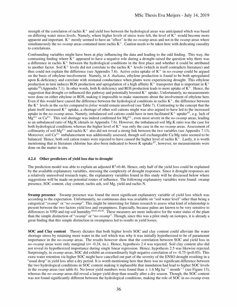
MSc Thesis Eva Meijers - July 14, 2019
strength of the correlation of rachis K+ and yield loss between the hydrological areas was anticipated which was basedon differing water stress levels. Namely, where higher levels of stress were felt, the level of K+ would become moreapparent and important. K+ mostly seemed to have an "effect" in the no-swamp areas and not in the swamp areas wheresimultaneously the no-swamp areas contained more rachis K+. Caution needs to be taken here with dedicating causalityto correlations.
Confounding variables might have been at play influencing the data and leading to the odd finding. This way, thecontrasting finding where K+ appeared to have a negative role during a drought raised the question why there wasa difference in rachis K+ between the hydrological conditions in the first place and whether it could be attributedto another factor. Soil K+ levels did not correlate to the rachis K+ levels (which in itself contradicts literature) andthus could not explain the difference (see Appendix 7.6). Active extra uptake of K+ in no-swamp could be arguedon the basis of ethylene involvement. Namely, in A. thaliana, ethylene production is found to be both upregulatedupon K-deficiency and correlate with stomatal conductance when plants were experiencing drought. This ethyleneproduction in turn induces ROS production and upregulation of a high affinity K+ transporter that is important in K+
uptake83(Appendix 7.1). In other words, both K-deficiency and ROS production leads to more uptake of K+. Hence, thesuggestion that drought co-influenced this pathway and potentially boosted K+ uptake. Unfortunately, no measurementswere done on either ethylene or ROS, making it impossible to make statements about the involvement of ethylene here.Even if this would have caused the difference between the hydrological conditions in rachis K+, the difference betweenthe K+ levels in the rachis compared to foliar would remain unsolved (see Table 7). Contrasting to the concept that theplant itself increased K+ uptake, a shortage of other soil cations might was also argued to have led to the increaseduptake in the no-swamp areas. Namely, imbalanced soil cations could have in turn facilitated K+ uptake67, e.g. lack ofMg2+ or Ca2+. This soil shortage was indeed confirmed for Mg2+, even most severe in the no-swamp areas, leadingto an unbalanced ratio of Mg:K (details in Appendix 7.6). However, the imbalanced soil Mg:K ratio was the case forboth hydrological conditions whereas the higher level of K+ was only the case in the no-swamp areas. Assessment ofcollinearity of soil Mg2+ and rachis K+ also did not reveal a strong link between the two variables (see Appendix 7.13).Moreover, soil Ca2+ imbalancement was additionally assessed, though soil exchangeable Ca:Mg ratio seemed to bebalanced. Hence, both soil cation routes were rejected to have caused the higher level of rachis K+. Lastly, it is worthmentioning that in literature chlorine has also been indicated to boost K uptake87, however, no measurements weredone on the matter in situ.
4.2.4 Other predictors of yield loss due to drought
The prediction model was able to explain an adjusted R2=0.46. Hence, only half of the yield loss could be explainedby the available explanatory variables, stressing the complexity of drought responses. Since it drought responses area relatively unresolved research topic, the explanatory variables found in this study will be discussed below wheresuggestions will be made on potential routes of influence. The following explanatory variables were found: swamppresence, SOC content, clay content, rachis ash, soil Mg, yield and rachis N.
Swamp presence Swamp presence was found the most significant explanatory variable of yield loss which wasaccording to the expectation. Unfortunately, no continuous data was available on “soil water level” other than being acategorical “swamp” or “no-swamp”. This might be interesting for future research to assess what kind of relationship ispresent between the two factors yield loss and swampiness. Especially, because palms are known to be very sensitive todifferences in VPD and top soil humidity49,61,64,92. These measures are more indicative for the water status of the plantthan the simple distinction of “swamp” or “no-swamp”. Though, since this was a pilot study on isotopes, it is already agreat finding that this simple distinction in swampiness led to results in yield losses.
SOC and Clay content Theory dictates that both higher levels SOC and clay content could alleviate the watershortage stress by retaining more water in the soil which was why it was initially hypothesized to be of paramountimportance in the no-swamp areas. The results however show that the correlation between SOC and yield loss inno-swamp areas were only marginal (r= -0.24, ns.). Hence, hypothesis 2.4 was rejected. Soil clay content also didnot reveal its hypothesized importance during single linear regression. Hence, hypothesis 2.5 was likewise rejected.Surprisingly, in swamp areas, SOC did exhibit an extraordinarily high negative correlation of r= -0.75 (p<0.05). Thisextra water retention via higher SOC might have cancelled out part of the severity of the ENSO drought resulting in a“usual drop” in yield loss after a dry period. It is worth mentioning here that there was no significant difference betweenthe two hydrological conditions in SOC content making it inplausible that inundation had lead to higher SOC levelsin the swamp areas (see table 6). No lower yield numbers were found than ± 1.6 Mg ha−1 month−1 (see Figure 13),whereas the no-swamp areas did reveal a larger yield drop than usually after a dry season. Though, the SOC contentwas not found significantly different between the hydrological conditions, making the role of SOC in no-swamp even
36

MSc Thesis Eva Meijers - July 14, 2019
more baffling and incomprehensible as it should have mostly aided the hydrological condition which suffered the mostfrom the drought.
Rachis ash Rachis ash was surprisingly found a rather powerful explanatory variable of yield loss, though not in theswamp areas. It correlated positively with yield loss, meaning that with more ash content in the rachis, more yieldloss was found. In short, rachis ash represents the quantity of inorganic salts and frond strands are indicated to havea rachis ash content of approximately 0.7%105. In this study, rachis ash levels of 4.01% and 4.57% were found forswamp and no-swamp, respectively. Reasons for this difference remain unknown. Though, notably, frond strands, likeother non-wood fibres, contain comparatively high ash contents, especially in the tropics. Variability in ash and mineralcontent can be substantial as it depends on genetic, environmental, physiological and morphological differences amongcrops116; e.g. leaves are generally much richer in ash content than reproductive organs and stems105 which was inagreement with this results of this study (see Figure 6)). To assess whether the inorganic constituents were translocatedto another organ in the swamp areas (explaining the mismatch with yield loss), foliar ash was assessed. The correlationbetween rachis ash and foliar ash was found negative though only marginal r= -0.21 (p-value not assessed). Therefore,the theory of translocation was rejected.
Interestingly, rachis ash showed an extraordinary strong correlation with the amount of rachis K+ in both databasesand both hydrological conditions. In particular the correlation in "All blocks" the combined conditions stands out aswith r=0.95(p was not assessed; see Appendix 7.13). The strength of the correlation between the two variables didnot seem to be affected by sample size nor hydrological condition. The high and significant correlation forms a solidbasis for collinearity between rachis ash and rachis K+. Here the origin of the word potassium becomes interestingas it is derived from pot ash which refers to plant ashes soaked in water in a pot, which was the primary means ofmanufacturing a pot before the industrial revolution. It might have been that the inorganic salts determining the rachisash composed mostly of inorganic salts containing K+. Interestingly, as earlier discussed, K+ was anticipated based ontheory to be involved in drought tolerance which was then confirmed in this study (though opposite role as expected).From multiple linear regression, rachis ash was found of utmost importance in predicting yield in the no-swamp areas,whereas rachis K+ was absent. Since the data set was not very large, it raises the question whether rachis ash canbe considered a proxy for rachis K+. Namely, the low number of data points might have resulted coincidentally in aslightly lower match of rachis K+ than rachis ash. If so, this collinearity finding makes a strong case to assume that theinfluence of rachis K+ might be stronger than expected. The fact that rachis ash was not a strong explanatory variablein the swamp areas (see Appendix 12) could also be explained by the fact that SOC and water availability compensatedfor the water shortage there which was severely noticed in the no-swamp. Future research on the relationship betweenrachis K+ and rachis ash is needed to make any convincing statements.
Soil Mg2+ The unexpected variable soil Mg2+ (antagonist of K+) popped up in the “All blocks” database whichseemingly could explain a large share of the variance in yield loss (r= -0.40 (p<0.05) and r= -0.51(p<0.05) for combinedareas and no-swamp areas) (see Table 8). Whatever the reason might be behind the earlier mentioned Mg2+ deficiency,this strong correlation suggest that Mg2+ levels somehow affected the palms during the drought in a positive wayhampering yield loss (the found opposite effect of K+). Mg2+ is known to be a central element in chlorophyll, phosphatemetabolism, plant respiration and activation of enzymes65,67. However, having too little Mg2+ would via this way leadto lower yield numbers in general, which was not the case for the no-swamp areas when sufficient rain was present as itwas comparable with the swamp areas (correlation Mg2+ yield was r=0.03 (p-value not assessed, combined all blocksdatabase). Based on this, Mg2+ is not assumed to fertilize the palms nor to lead to under-performance caused by totoo little Mg2+. Hence, Mg2+ seems to be only involved in yield loss and not in yield itself which is very unlikely.Notably, foliar and rachis Mg2+ did not show up in the top ten correlations to yield loss, making it questionable whetherthe presence of soil Mg2+ in the top ten was due to coincidence since plant Mg levels are more indicative for plantperformance. In case data is not influenced by coincidence, it might still be possible to partially explain the increasedyield loss in the no-swamp areas; namely when efficient photosynthesis, phosphate metabolism and plant respirationbecome crucial (lower than 100 mm month−1 of rain), the lack of sufficient Mg2+ could become vital to yield. Moreresearch is needed to confirm this additional effect during water shortage. The results of this study potentially entailthat applying more Mg2+ could lower the yield loss during a drought. This makes the predictor very interesting. Aconvincing pathway wherein Mg2+ positively affects palms during a drought remains unknown and should be lookedinto in future research.
Yield 2014 A rather convincing correlation was found between yield 2014 and yield loss with an r= -0.40 (p<0.05)(see Appendix 7.8). The autocorrelation between yield loss and yield in the previous year to the drought is not asurprising finding as a certain level of productivity comes with a corresponding level of internal assimilate cost. And,when yields are high, corresponding high maintenance costs are expected to lead to more deprivation of internal CO2
and water shortage which in turn translates into more yield loss. In terms of inflorescence during droughts, highly
37

MSc Thesis Eva Meijers - July 14, 2019
productive palms need to abort their highly demanding bunches leading to coherent aggravated yield losses. Strangely,correlation of yield 2014 and yield loss in swamp was found r= -0.13 (p>0.05,ns.). This is suggested to be due tooverruling/compensating factors such as SOC.
Rachis N Lastly, the link between rachis N and yield loss might be stomatal conductance, whereas unlikely via afertilizing effect since rachis and/or foliar N did not show strong nor positive correlations with yields. Frankly, mostlynegative correlations were found there. The link of rachis N and yield loss via stomatal conductance is supported bymultiple studies that also found a negative relationship between isotope discrimination and leaf N concentration35,36.The exact underlying mechanism however remains unknown. Unfortunately, no stomatal conductance measurementswere done that could proof this routes and isotopes measurements did not reveal its expected pattern which couldalternatively have been a proxy for stomatal conductance. It is worth mentioning that N levels were never deficient inthis study (see Figure 6), therefore the correlation might even have been stronger when more severe differences wouldhave been available in N concentrations. Further research might elucidate the found connection.
4.3 Part III Link isotope and yield analysis
The title of this paper "Detecting potassium mediated drought responses in oil palm (Elaeis guineensis): an isotopicstudy on frond bases" suggests that isotopes might be helpful in investigating the yield losses due to drought responses.Yield numbers of course not solely reflect stomatal conductance thus caution should be taken when interpreting thedifferences between the yield and isotope analysis. Indeed, inconsistencies were found between the two analyses, forexample: the yield numbers confirmed the severe drought at the start of 2016, however, the isotopes alluded to thecontrary. Secondly, from the yield analysis, swamp presence seemed to be the most important explanatory variablefor yield losses which was not the case for the isotopes analysis where soil total P was found most important. Theconfounding effect of swamp presence on soil total P was subsequently not confirmed in the yield analysis. Thirdly, thefinding in the isotope analysis of a delay in the swamp areas in response to the drought compared to the no-swamp areaswas not supported when yield numbers were investigated. Lastly, the finding of the significant role of K+ in the yieldanalysis was not confirmed in the isotope analysis where it was hypothesized to more apparent due to the direct linkwith stomatal conductance. Hence, the proposed new method of using isotopes of frond base tissue of oil palms stillfaces some difficulties in its applicability in investigating stomatal conductance during droughts.
5 Concluding remarks
From the isotope analysis is was found that the isotope measurements did not reveal the hypothesized peak norseasonality. It did reveal that higher levels of soil moisture lead to more discrimination against the heavier isotope.Potassium did not show its hypothesized role via stomatal closure when it was correlated to the isotopes. Suggestionswere made that the distorted isotope signal was due to utilization of non-structural carbohydrates, alternative whole-wood components, timing of the hardening of the frond bases, exhausts of a close by mill or local decomposition &respiration rates. The nutrient phosphorus was found to strongly correlate to the isotopes, however, this is suggested tobe due to a confounding effect of the hydrological conditions or pH. Measurements on the isotopes were insightful byadding to the current state of the art on carbon isotope ratios as the data reflected a high-resolution intra-annual timeseries containing a drought of carbon isotopes in a tropical plant.
From the yield analysis, a difference was found in yield loss inferred by the ENSO between the chosen hydrologicalconditions, where the drier condition significantly suffered more. Potassium did reveal its importance in the yieldloss analysis, however, its role seemed to be detrimental to the palms during the drought which remains unresolved.Higher levels of soil organic carbon nor clay content seemed to aid the more severely water deprived areas. The palmsparticularly revealed yield losses when precipitation levels dropped below 100 mm month−1. Contrary to the literature,the wetter areas revealed similar yields as the drier areas, suggesting no negative effect from temporal submergence.The higher levels of K+ in the drier areas are suggested to be due to higher levels of ROS (reactive oxygen species)production as a result of the drought which in turn might have stimulated more uptake of K+. Variables that mightbe insightful to look into in future research on drought responses are swamp presence, rachis ash, soil Mg, yield andrachis N. The rachis ash content is suggested to be proxies for K+ levels based on collinearity analysis. Hopefully,the outcomes of the single and multiple regression models may serve as starting points for further analysis into plantsdrought responses.
38
MSc Thesis Eva Meijers - July 14, 2019
6 Recommendations for further research
In future research on carbon isotopes in monocotyledons, the components of the whole-wood sample should be assessed,e.g. lignin, cellulose, glucose. This could be done by assessing the contents of bulky whole-wood samples at least oncein triplicate to get a rough idea. Secondly, research on sugar flows between organs could be valuable for understandingthe storage and/or usage of reserves in monocotyledons. Quantitative information on the abundance of photo-assimilatestored in a previous year, carried over to the next, and remobilized in the dry season would be useful to understandand interpret isotope dendro-climatological data accurately in future research45. The labelled sugar type that shouldbe measured would be glucose, as oil palm is one of the rare species that uses glucose (53%) mainly as a transitoryreserve carbohydrate, followed by sucrose and starch (20% each)46. Sugar flows could be investigated by measuringthe level NSC within palms in, at least, the stem. Namely, NSC is mainly stored in the stem (65%), followed by theleaves (17%), “persistent leaf bases” (13%), and little in the roots (2%)46. It is worth mentioning that the top part of thestem in oil palms generally contain relatively more starch than the lower part (20 mg g−1 versus less than 5 mg g−1)which translates in a lower (smaller) isotope ratio signature. This starch storage could have resulted in a systematicerror of overestimation of the carbon isotopes, which was not the case considering isotope ratios of -29h were foundon average whereas starch is 25-26h. It is advisable to assess the stability of Cair surrounding the sampled palms.Levels of turbulence might become insightful with regard to the size of the boundary layer. Since recurring dryingand wetting events are known to influence decomposition- and respiration rates, isotope values might be affected by itand oil palm is often grown on peat soil (high water content). Therefore, assessment of these processes should not beoverlooked. The preliminary suggestion that hardening of fronds might affect the found isotopes could be an interestingnew topic for plant physiology. Research on the influence of phosphorus in isotopes could help elucidate the foundcorrelation with the isotopes in case it is not due to collinearity with swampiness. Phosphorus might be important indrought tolerance via mesophyll thickness, and with that, diffusion of CO2 to the carboxylation site. For this research,data on RuBisCO activity with corresponding plant P status would be insightful. Research on the influence of N onstomatal conductance during droughts might be insightful as literature states that lower levels of N coincide with higherdiscrimination against 13C. These N levels might interfere with isotope results when isotopes are used as a proxy forstomatal conductance.
Research on the influence of the nutrient K+ during a drought could be analysed more thoroughly as it was found to beimportant in yield loss. The current finding of K+ having a potential negative effect during droughts by enhancing yieldlosses in oil palm might have large implications for palm oil production via K+ fertiliser application. More severelyK-deficient palms should be used with coherent hydrological condition (potentially a factorial design) in combinationwith research on the level of ethylene and ROS and K+ uptake during drought. Notably, this is difficult due to thefact oil plantations or large scale companies are usually under strict nutrient management (applying sufficient K+) tooptimize yield. K-deficiency is found more often in small scale companies where maintenance is frequently not equalbetween blocks and/or other managerial effects might influence the data. On top of that, oil palm is a perennial cropand responds only slowly to new hydrological conditions, making it prone to varying managements over time. WhenK-deficient areas are not available, maybe there lies an opportunity in searching for blocks where soil nutrients areextremely misbalanced leading to very little uptake of K+, e.g. areas where Ca2+ and Mg2+ are available in largeamounts. In case carbon isotopes are used as a proxy for stomatal conductance in oil palm using frond bases, gatheringmore data points of corresponding δ13C and nutrient/sugar levels would extremely valuable.
Future research should be done on differences in yield loss in varying hydrological conditions as they might be importantfor choice of future investments of plantations as they are currently frequently located on peat soils. In such research,VPD, top soil humidity and SOC should be assessed. These measures are more indicative for the water status of theplant than the binary distinction of “swamp” or “no-swamp”. To confirm whether palms truly under water shortagestress, root ethylene exudates, root oxygen levels and leaf turgor pressure could be insightful83. It might elucidate whatkind of relationship is present between the two factors yield loss and swampiness. Research on the influence of Mg2+
in oil palms might be valuable as a lack of sufficient Mg2+ turned out to increase yield losses during drought. Thismakes the predictor very interesting for nutrient management of plantations.
39

MSc Thesis Eva Meijers - July 14, 2019
References[1] Malaysian Palm Oil Board. Monthly palm oil trade statistics. 2016.
[2] W Gerritsma and FX Soebagyo. An analysis of the growth of leaf area of oil palms in indonesia. ExperimentalAgriculture, 35(3):293–308, 1999.
[3] RK Pachauri et al. Climate change 2014: synthesis report. Contribution of Working Groups I, II and III to thefifth assessment report of the Intergovernmental Panel on Climate Change. IPCC, 2014.
[4] UNFCCC. Adoption of the paris agreement. Report CP, 9(1), 2015.
[5] AA Yusuf and H Francisco. Climate change vulnerability mapping for southeast asia. 2009.
[6] J Caliman and A Southworth. Effect of drought and haze on the performance of oil palm. 1998.
[7] A Dai. Drought under global warming: a review. Wiley Interdisciplinary Reviews: Climate Change, 2(1):45–65,2011.
[8] Z Sa’adi et al. Projection of spatial and temporal changes of rainfall in sarawak of borneo island using statisticaldownscaling of cmip5 models. Atmospheric research, 197:446–460, 2017.
[9] R Garreaud and DS Battisti. Interannual (enso) and interdecadal (enso-like) variability in the southern hemispheretropospheric circulation. Journal of Climate, 12(7):2113–2123, 1999.
[10] BK Linsley et al. Decadal sea surface temperature variability in the subtropical south pacific from 1726 to 1997ad. Science, 290(5494):1145–1148, 2000.
[11] MN Evans et al. Support for tropically-driven pacific decadal variability based on paleoproxy evidence.Geophysical Research Letters, 28(19):3689–3692, 2001.
[12] PF Poussart et al. Resolving seasonality in tropical trees: multi-decade, high-resolution oxygen and carbonisotope records from indonesia and thailand. Earth and Planetary Science Letters, 218(3-4):301–316, 2004.
[13] JN Egilla et al. Drought stress influences leaf water content, photosynthesis, and water-use efficiency of hibiscusrosa-sinensis at three potassium concentrations. Photosynthetica, 43(1):135–140, 2005.
[14] E Lamade et al. Changes in 13c/12c of oil palm leaves to understand carbon use during their passage fromheterotrophy to autotrophy. Rapid Communications in Mass Spectrometry: An International Journal Devoted tothe Rapid Dissemination of Up-to-the-Minute Research in Mass Spectrometry, 23(16):2586–2596, 2009.
[15] GD Farquhar et al. Carbon isotope discrimination and photosynthesis. Annual review of plant biology, 40(1):503–537, 1989.
[16] TE Dawson et al. Stable isotopes in plant ecology. Annual review of ecology and systematics, 33(1):507–559,2002.
[17] MM Barbour. Stable oxygen isotope composition of plant tissue: a review. Functional Plant Biology, 34(2):83–94, 2007.
[18] P van der Sleen et al. Stable isotopes in tropical tree rings: theory, methods and applications. Functional ecology,31(9):1674–1689, 2017.
[19] D McCarroll and NJ Loader. Stable isotopes in tree rings. Quaternary Science Reviews, 23(7-8):771–801, 2004.
[20] LA Cernusak et al. Environmental and physiological determinants of carbon isotope discrimination in terrestrialplants. New Phytologist, 200(4):950–965, 2013.
[21] GD Farquhar and RA Richards. Isotopic composition of plant carbon correlates with water-use efficiency ofwheat genotypes. Functional Plant Biology, 11(6):539–552, 1984.
[22] LA Cernusak et al. Physiological and isotopic (δ13c and δ18o) responses of three tropical tree species to waterand nutrient availability. Plant, Cell & Environment, 32(10):1441–1455, 2009.
[23] JR Ehleringer and TA Cooper. Correlations between carbon isotope ratio and microhabitat in desert plants.Oecologia, 76(4):562–566, 1988.
[24] JR Ehleringer. Carbon and water relations in desert plants: an isotopic perspective. In Stable isotopes and plantcarbon-water relations, pages 155–172. Elsevier, 1993.
[25] N Buchmann and JR Ehleringer. Co2 concentration profiles, and carbon and oxygen isotopes in c3 and c4 cropcanopies. Agricultural and Forest Meteorology, 89(1):45–58, 1998.
[26] RL Korol et al. Effects of water status and soil fertility on the c-isotope signature in pinus radiata. TreePhysiology, 19(9):551–562, 1999.
40

MSc Thesis Eva Meijers - July 14, 2019
[27] J Ma et al. Variation in the stable carbon and nitrogen isotope composition of plants and soil along a precipitationgradient in northern china. PloS one, 7(12):e51894, 2012.
[28] S Madhavan et al. Effects of relative humidity on carbon isotope fractionation in plants. Botanica Acta,104(4):292–294, 1991.
[29] JR Ehleringer et al. Seasonal variation in the carbon isotopic composition of desert plants. Functional Ecology,pages 396–404, 1992.
[30] JA Panek and RH Waring. Stable carbon isotopes as indicators of limitations to forest growth imposed by climatestress. Ecological Applications, 7(3):854–863, 1997.
[31] JR Ehleringer et al. Leaf carbon isotope and mineral composition in subtropical plants along an irradiance cline.Oecologia, 70(4):520–526, 1986.
[32] JK Zimmerman and JR Ehleringer. Carbon isotope ratios are correlated with irradiance levels in the panamanianorchid catasetum viridiflavum. Oecologia, 83(2):247–249, 1990.
[33] JM Welker et al. Leaf carbon isotope discrimination and vegetative responses of dryas octopetala to temperatureand water manipulations in a high arctic polar semi-desert, svalbard. Oecologia, 95(4):463–469, 1993.
[34] JA Panek and RH Waring. Carbon isotope variation in douglas-fir foliage: improving the δ13c–climaterelationship. Tree Physiology, 15(10):657–663, 1995.
[35] AG Condon et al. The effect of variation in soil water availability, vapour pressure deficit and nitrogen nutritionon carbon isotope discrimination in wheat. Australian Journal of Agricultural Research, 43(5):935–947, 1992.
[36] J Guehl et al. Differential response of leaf conductance, carbon isotope discrimination and water-use efficiencyto nitrogen deficiency in maritime pine and pedunculate oak plants. New Phytologist, 131(2):149–157, 1995.
[37] WD Bowman et al. Short-term changes in leaf carbon isotope discrimination in salt-and water-stressed c4grasses. Plant Physiology, 90(1):162–166, 1989.
[38] DR Sandquist and JR Ehleringer. Carbon isotope discrimination in the c shrub atriplex confertifolia along asalinity gradient. The Great Basin Naturalist, pages 135–141, 1995.
[39] JA Poss et al. Stable carbon isotope discrimination: an indicator of cumulative salinity and boron stress ineucalyptus camaldulensis. Tree physiology, 20(16):1121–1127, 2000.
[40] I Bettarini et al. Isotopic carbon discrimination and leaf nitrogen content of erica arborea l. along a co2concentration gradient in a co2 spring in italy. Tree Physiology, 15(5):327–332, 1995.
[41] JR Ehleringer and TE Cerling. Atmospheric co2 and the ratio of intercellular to ambient co2 concentrations inplants. Tree Physiology, 15(2):105–111, 1995.
[42] DG Williams et al. Carbon isotope discrimination by sorghum bicolor under co2 enrichment and drought. Newphytologist, 150(2):285–293, 2001.
[43] A Gessler et al. Stable isotopes in tree rings: towards a mechanistic understanding of isotope fractionation andmixing processes from the leaves to the wood. Tree physiology, 34(8):796–818, 2014.
[44] G Helle et al. Interpreting climate proxies from tree-rings. In The Climate in Historical Times, pages 129–148.Springer, 2004.
[45] A Kagawa et al. 13co2 pulse-labelling of photoassimilates reveals carbon allocation within and between treerings. Plant, Cell & Environment, 29(8):1571–1584, 2006.
[46] S Legros et al. Carbohydrates reserves in 9 year old oil palm: nature, distribution and seasonal changes. Optimumuse of resources: challenges and opportunities for sustainable oil palm development. IOPC Bali, 2006.
[47] E Fichtler et al. Stable-carbon isotope time series from tropical tree rings indicate a precipitation signal. Tree-RingResearch, 66(1):35–50, 2010.
[48] JR Ehleringer et al. Carbon isotope discrimination and transpiration efficiency in common bean. Crop Science,31(6):1611–1615, 1991.
[49] E Legros et al. Role of transitory carbon reserves during adjustment to climate variability and source–sinkimbalances in oil palm (elaeis guineensis). Tree Physiology, 29(10):1199–1211, 2009.
[50] OECD and FAO. Oilseed and oilseed products: Agricultural outlook, 2013.
[51] EB Fitzherbert et al. How will oil palm expansion affect biodiversity? Trends in ecology & evolution,23(10):538–545, 2008.
41

MSc Thesis Eva Meijers - July 14, 2019
[52] V Vijay et al. The impacts of oil palm on recent deforestation and biodiversity loss. PloS one, 11(7):e0159668,2016.
[53] LS Woittiez et al. Yield gaps in oil palm: A quantitative review of contributing factors. European Journal ofAgronomy, 83:57–77, 2017.
[54] RHV Corley. How much palm oil do we need? Environmental Science & Policy, 12(2):134–139, 2009.
[55] LP Koh et al. Remotely sensed evidence of tropical peatland conversion to oil palm. Proceedings of the NationalAcademy of Sciences, 108(12):5127–5132, 2011.
[56] RHV Corley and TK Hong. Irrigation of oil palms in malaysia. In International Conference on Oil Palm inAgriculture in the Eighties, Kuala Lumpur (Malaysia), 17-20 Jun 1981. PPP (ISP), 1982.
[57] IE Henson and KC Chang. Evidence for water as a factor limiting performance of field palms in west malaysia.In Proceedings of 1989 PORIM International Palm Oil Development Conference–Agriculture, pages 487–498,1990.
[58] K Thirumalai et al. Extreme temperatures in southeast asia caused by el niño and worsened by global warming.Nature communications, 8:15531, 2017.
[59] NN Kamil and SF Omar. The impact of el niño and la niña on malaysian palm oil industry. Oil Palm Bulletin,74:1–6, 2017.
[60] CWS Hartley. The oil palm longman, 1988.
[61] I Henson et al. The influence of climatic conditions on gas and energy exchanges above a young oil palm standin north kedah, malaysia. Journal of oil palm Research, 17(C):73, 2005.
[62] MM Chaves et al. Understanding plant responses to drought—from genes to the whole plant. Functional plantbiology, 30(3):239–264, 2003.
[63] OS Lau. Stomata. eLS, 2018.
[64] E Dufrene and B Saugier. Field studies of leaf gas exchanges in oil palm tree (elaeis guineensis jacq.). InAnnales des Sciences Forestières, volume 46, pages 439s–442s. EDP Sciences, 1989.
[65] RHV Corley and CK Mok. Effects of nitrogen, phosphorus, potassium and magnesium on growth of the oilpalm. Experimental Agriculture, 8(4):347–353, 1972.
[66] CJ Breure. Development of leaves in oil palm (elaeis guineensis) and determination of leaf opening rate.Experimental Agriculture, 30(4):467–472, 1994.
[67] I Rankine and TH Fairhurst. Management of phosphorus, potassium and magnesium in mature oil palm. BetterCrops International, 13(1):11, 1999.
[68] Gas exchange of excised oil palm {Elaeis guineensis) Fronds, author=Hamff, MH, journal=Asian Journal ofPlant Sciences, volume=5, number=1, pages=9–13, year=2006.
[69] K Suresh et al. Changes in photosynthetic activity in five common hybrids of oil palm (elaeis guineensis jacq.)seedlings under water deficit. Photosynthetica, 50(4):549–556, 2012.
[70] D Cros et al. Differential response to water balance and bunch load generates diversity of bunch productionprofiles among oil palm crosses (elaeis guineensis). Tropical plant biology, 6(1):26–36, 2013.
[71] USDA. Malaysia: El nino takes a bite out of 2015/16 palm oil production. Foreign Agricultural Service-Commodity Intelligence Report, 2016.
[72] P Silva et al. Drought tolerance in two oil palm hybrids as related to adjustments in carbon metabolism andvegetative growth. Acta physiologiae plantarum, 39(2):58, 2017.
[73] UR Sangakkara et al. Effect of soil moisture and potassium fertilizer on shoot water potential, photosynthesisand partitioning of carbon in mungbean and cowpea. Journal of Agronomy and Crop Science, 185(3):201–207,2000.
[74] RA Fischer and TC Hsiao. Stomatal opening in isolated epidermal strips of vicia faba. ii. responses to kclconcentration and the role of potassium absorption. Plant Physiology, 43(12):1953–1958, 1968.
[75] A Gupta et al. Maintenance of photosynthesis at low leaf water potential in wheat: role of potassium status andirrigation history. Plant Physiology, 89(4):1358–1365, 1989.
[76] I Cakmak. The role of potassium in alleviating detrimental effects of abiotic stresses in plants. Journal of PlantNutrition and Soil Science, 168(4):521–530, 2005.
42

MSc Thesis Eva Meijers - July 14, 2019
[77] M Aslam et al. Drought tolerance in maize through potassium: Drought stress, its effect on maize productionand development of drought tolerance through potassium application. Cercetari Agronomice În Moldova, XLVI,16, 2013.
[78] P Battie-Laclau et al. Effects of potassium and sodium supply on drought-adaptive mechanisms in eucalyptusgrandis plantations. New Phytologist, 203(2):401–413, 2014.
[79] K Mengel. Kirkby ea: 2001. principles of plant nutrition.
[80] M Wang et al. The critical role of potassium in plant stress response. International journal of molecular sciences,14(4):7370–7390, 2013.
[81] I Cakmak et al. Changes in phloem export of sucrose in leaves in response to phosphorus, potassium andmagnesium deficiency in bean plants. Journal of Experimental Botany, 45(9):1251–1257, 1994.
[82] P Gajdanowicz et al. Potassium (k+) gradients serve as a mobile energy source in plant vascular tissues.Proceedings of the National Academy of Sciences, 108(2):864–869, 2011.
[83] DP Schachtman. The role of ethylene in plant responses to k+ deficiency. Frontiers in plant science, 6:1153,2015.
[84] E Martineau et al. The effects of potassium nutrition on water use in field-grown maize (zea mays l.). Environ-mental and experimental botany, 134:62–71, 2017.
[85] DH Putranto. Stomatal Conductance and Chlorophyll Fluorescence of Oil Palm under Field Conditions. PhDthesis, MSc thesis, Wageningen University, Wageningen, 2018.
[86] MJ Webb et al. Site-specific fertilizer recommendations for oil palm smallholders using information from largeplantations. Journal of Plant Nutrition and Soil Science, 174(2):311–320, 2011.
[87] B Dubos et al. Potassium uptake and storage in oil palm organs: the role of chlorine and the influence of soilcharacteristics in the magdalena valley, colombia. Nutrient cycling in agroecosystems, 89(2):219–227, 2011.
[88] RHV Corley and PHB Tinker. Diseases of the oil palm. The Oil Palm, 5th edition. Chichester: Wiley Blackwell,pages 399–437, 2016.
[89] RHV Corley and BS Gray. Growth and morphology: Development in crop science (1), oil palm research, 1976.
[90] AFM Broekmans. Growth, flowering and yield of the oil palm in nigeria. JW Afric. Inst. for Oil Palm Res,2(7):187–220, 1957.
[91] O Dufour et al. Description of a simplified method of production forecasting in oil palm plantations based onclimatology. Oléagineux (Paris), 43(7):271–282, 1988.
[92] B Cornaire et al. Oil palm performance under water stress. background to the problem, first results and researchapproaches. Oléagineux (Paris), 49(1):1–12, 1994.
[93] RHV Corley and CJ Breure. Fruiting activity, growth and yield of oil palm. i. effects of fruit removal. Experi-mental Agriculture, 28(1):99–109, 1992.
[94] O’Leary and H Marion. Carbon isotopes in photosynthesis. Bioscience, 38(5):328–336, 1988.
[95] H Lambers et al. Plant physiological ecology. Springer Science & Business Media, 2008.
[96] RJ Francey and GD Farquhar. An explanation of 13 c/12 c variations in tree rings. Nature, 297(5861):28, 1982.
[97] DM Diez et al. OpenIntro statistics. OpenIntro, 2012.
[98] SW Leavitt and A Lone. Seasonal stable-carbon isotope variability in tree rings: possible paleoenvironmentalsignals. Chemical Geology: Isotope Geoscience Section, 87(1):59–70, 1991.
[99] A Verheyden et al. Annual cyclicity in high-resolution stable carbon and oxygen isotope ratios in the wood ofthe mangrove tree rhizophora mucronata. Plant, Cell & Environment, 27(12):1525–1536, 2004.
[100] GD Farquhar and LA Cernusak. Ternary effects on the gas exchange of isotopologues of carbon dioxide. Plant,Cell & Environment, 35(7):1221–1231, 2012.
[101] HC Fritts. Tree rings and climate. Elsevier, 2012.
[102] TT Kozlowski. Carbohydrate sources and sinks in woody plants. The botanical review, 58(2):107–222, 1992.
[103] S Borella et al. Reducing uncertainties in δ13c analysis of tree rings: Pooling, milling, and cellulose extraction.Journal of Geophysical Research: Atmospheres, 103(D16):19519–19526, 1998.
[104] NJ Loader et al. Comparison of stable carbon isotope ratios in the whole wood, cellulose and lignin of oaktree-rings. Palaeogeography, Palaeoclimatology, Palaeoecology, 196(3-4):395–407, 2003.
43

MSc Thesis Eva Meijers - July 14, 2019
[105] WD Wanrosli et al. Pulp from oil palm fronds by chemical processes. Industrial crops and products, 25(1):89–94,2007.
[106] LB Turner. Changes in the phosphorus content of capsicum annuum leaves during water stress. Journal of plantphysiology, 121(5):429–439, 1985.
[107] WA Payne et al. Effects of phosphorus and water supply on yield, transpirational water-use efficiency, andcarbon isotope discrimination of pearl millet. Crop Science, 40(1):120–125, 2000.
[108] N Sekiya and K Yano. Stomatal density of cowpea correlates with carbon isotope discrimination in differentphosphorus, water and co2 environments. New Phytologist, 179(3):799–807, 2008.
[109] RN Sah and DS Mikkelsen. Phosphorus behavior in flooded-drained soils. i. effects on phosphorus sorption.Soil science society of America Journal, 53(6):1718–1722, 1989.
[110] A Meijide et al. Controls of water and energy fluxes in oil palm plantations: Environmental variables and oilpalm age. Agricultural and Forest Meteorology, 239:71–85, 2017.
[111] MKV Carr. The water relations and irrigation requirements of oil palm (elaeis guineensis): a review. ExperimentalAgriculture, 47(4):629–652, 2011.
[112] IE Henson et al. Some observations on the effects of high water tables and flooding on oil palm, and a preliminarymodel of oil palm water balance and use in the presence of a high water table. Oil Palm Bulletin, 56:14–22,2008.
[113] KC Teoh et al. Potassium in the oil palm eco-system and some implications to manuring practice. In InternationalOil Palm/Palm Oil Conferences-Progress and Prospects 1987-Conference 1: Agriculture, Kuala Lumpur, 23-26Jun 1988. IPMKSM, 1988.
[114] HL Foster and NE Prabowo. Partition and transfer of nutrients in the reserve tissues and leaves of oil palm. InWorkshop on Nutrient Needs in Oil Palm, pages 17–18. IPNI Singapore, 2006.
[115] NE Prabowo et al. Prediction of expected yields of oil palm from the weights of leaf nutrients. 2011.
[116] A Monti et al. Mineral composition and ash content of six major energy crops. Biomass and Bioenergy,32(3):216–223, 2008.
[117] K Mengel and W Arneke. Effect of potassium on the water potential, the pressure potential, the osmotic potentialand cell elongation in leaves of phaseolus vulgaris. Physiologia plantarum, 54(4):402–408, 1982.
[118] A Lebaudy et al. Plant adaptation to fluctuating environment and biomass production are strongly dependent onguard cell potassium channels. Proceedings of the National Academy of Sciences, 105(13):5271–5276, 2008.
[119] PJ White. Improving potassium acquisition and utilisation by crop plants. Journal of Plant Nutrition and SoilScience, 176(3):305–316, 2013.
[120] O Arquero et al. Potassium starvation increases stomatal conductance in olive trees. HortScience, 41(2):433–436,2006.
[121] E Peiter. The plant vacuole: emitter and receiver of calcium signals. Cell calcium, 50(2):120–128, 2011.
[122] MG Lindhauer. Influence of k nutrition and drought on water relations and growth of sunflower (helianthusannuus l.). Zeitschrift für Pflanzenernährung und Bodenkunde, 148(6):654–669, 1985.
[123] CW Bednarz et al. Leaf photosynthesis and carbon isotope discrimination of cotton in response to potassiumdeficiency. Environmental and Experimental Botany, 39(2):131–139, 1998.
[124] María Benlloch-González et al. K+ starvation inhibits water-stress-induced stomatal closure. Journal of plantphysiology, 165(6):623–630, 2008.
[125] DE Peaslee and DN Moss. Photosynthesis in k-and mg-deficient maize (zea mays l.) leaves 1. Soil ScienceSociety of America Journal, 30(2):220–223, 1966.
[126] MR Dhakal and L Erdei. Long-term effects of abscisic acid on k+ transport in young wheat plants of different k+status. Physiologia Plantarum, 68(4):637–640, 1986.
[127] H Tomemori et al. Interactive effects of sodium and potassium on the growth and photosynthesis of spinach andkomatsuna. Plant production science, 5(4):281–285, 2002.
[128] SH Jin et al. Effects of potassium supply on limitations of photosynthesis by mesophyll diffusion conductance incarya cathayensis. Tree physiology, 31(10):1142–1151, 2011.
[129] M Ashraf et al. Growth and photosynthetic characteristics in pearl millet under water stress and differentpotassium supply. Photosynthetica, 39(3):389–394, 2001.
44

MSc Thesis Eva Meijers - July 14, 2019
[130] B Basile et al. Leaf potassium concentration, co2 exchange and light interception in almond trees (prunus dulcis(mill) da webb). Scientia Horticulturae, 98(2):185–194, 2003.
[131] TR Peoples and DW Koch. Role of potassium in carbon dioxide assimilation in medicago sativa l. Plantphysiology, 63(5):878–881, 1979.
[132] J Flexas et al. Mesophyll diffusion conductance to co2: an unappreciated central player in photosynthesis. PlantScience, 193:70–84, 2012.
45
MSc Thesis Eva Meijers - July 14, 2019
7 Appendices
7.1 In depth role of K+
Most importantly, K+ is a crucial osmoticum and the main cation that is available in soluble form responsible for leafwater potential79,117,118. It acts as the main determinant of cell turgor influencing leaf elongation and leaf area119.
Secondly, K+ is the osmotic driving force of water influx into guard cells (see Figure 2), with that regulating stomatalopening and closure120,121. Guard cells take up K+ ions by active transport which simultaneously leads to water enteringthe cell by osmosis. Since the guard cell walls are unevenly thickened, the cells then start to bow by turgidity; openingthe stomata. When K+ ions are then pumped out of the cell, water follows again by osmosis and the stomata close79. Itis known that insufficient K+ levels can impair stomatal conductance, meaning that stomatal opening and/or closingis retarded or the stomatal aperture is too wide. Depending on the species, K+ can either lead to impaired stomatalclosure78,122–124 or impaired stomatal opening125–128. Though, some studies did not find any effect on the stomatalmechanism under K-deficiency129–131. In response, Putranto85 investigated what was true for oil palm by investigatingstomatal conductance. Impaired stomatal conductance was indeed recorded in K-deficient plants in the afternoon;only K-sufficient oil palms showed significantly lower stomatal conductance during the afternoon period than in themorning. Lower stomatal conductance can be both caused by retarded opening or a too small opening of the guard cells.Notably, the stomatal conductance was recorded while no real acute water shortage occurred during the study; the resultsolely reflects the reaction to air drying. Putranto also found that in the morning the variability in stomatal conductancewas much higher in the K-deficient hydrological condition than in the K-sufficient hydrological condition, with themajority of the stomatal conductance values in the lower half of the range. This could be due to the large variability thatno significantly lower stomatal conductance was found in the K-deficient palms over the course of the day, makingthe aforementioned impaired stomatal conductance incorrect. Moreover, there were large differences in severity inK+-deficiency within the plot, which could explain the large variability. In other words, no indisputable evidence yetcame out to confirm what the effect is at stomatal level in K+ deficient palms.
Thirdly, K-deficiency has been found to increase mesophyll resistance by thickening of leaves78. Namely, in eucalyptus,K-deficient leaves have thinner palisade and spongy layers, less intercellular space and smaller paracytic stomata. Thisincreases mesophyll resistance. This complicates CO2 to reach Rubisco132. In case of a drought, stomata close fully orat least partially upon water shortage leading to a internal shortage of CO2. When palms are then also deficient in K+,CO2 shortage could be aggravated due to the increased mesophyll resistance over which CO2 has to pass. In line withthis, RuBisCO activity is recorded to increase by K+ fertilization in various species78.
K+ eliminates damaging reactive oxygen species (ROS) released upon a water deficit period76. ROS are producedwhen there is an excess of energy from the photosystems (I and II) which can not be used in CO2 fixation because itexceeds the capacity of the chloroplasts76. This excess of energy is then alternatively used for activation of O2 to ROSat the expense of CO2 fixation. This occurs during environmental stressors such as drought, chilling, deficiency ofnutrients and salinity, especially in combination with high light intensities or long-term sunlight conditions77. TheseROS damage the chloroplasts, cell membranes lipids, enzyme proteins and nucleic acids76, hampering the overallproductivity. ROS ultimately results in upregulation of a high affinity K+ transporter of K that is important in uptake.
At the roots, K+ appears to have a positive affect as well; it promotes deep root exploration and general root growth83,84).When there is a deficiency in K+, a cascade of reactions take place which result in higher affinity to take up K+, roothair growth and primary lateral root growth (see Figure 1 Schachtman83. In A.thaliana ethylene has been found tobe upregulated upon K-deficiency and correlate with stomatal conductance when plants were droughted83. Ethyleneproduction then induces ROS which ultimately results in upregulation of a high affinity K+ transporter of K+ that isimportant in uptake.
Lastly, K+ plays an important role in photosynthate loading into the phloem sap78,81,82. Photosynthate loading intothe phloem sap could serve as a Non-Structural Carbon (NSC) reserve in times of shortage, e.g. a drought46. Sucroseexport from the leaves to the phloem exudate was found to be drastically decreased by K-deficiency in bean81. However,contrasting data between species have been found in response to K+ fertilization and starch concentrations78.
46

MSc Thesis Eva Meijers - July 14, 2019
7.2 Maps Estate Lambir 2 (SOPB)
Three maps were made available by SOPB: Topography, Swamp areas and a semi-detailed soil map.
Figure 15: Topography Map Lambir Estate 2. SOPB
Figure 16: Swamp areas: Map Lambir Estate 2. SOPB
47

MSc Thesis Eva Meijers - July 14, 2019
Figure 17: Semi-detailed soil mail. Map Lambir Estate 2. SOPB
7.3 Environment of chosen palms
For reference, a photograph was taken of all the chosen palms.
48

MSc Thesis Eva Meijers - July 14, 2019
Figure 18: Palms on dry soils
Figure 19: Swampy soils
49

MSc Thesis Eva Meijers - July 14, 2019
7.4 Appendix Used Sampling Protocol at Sarawak Oil Palm Berhad, Lambir Estate
Requirements for in the field
• Map of the Lambir Estate 2
• Electric drill
• Metal brush for cleaning the hole saw bits between the samples
• Sharpener for the hole saw bits
• Hole saw bits (2 in case of potential break down)
• Two batteries
• Double ladder
• Plastic canvas for on the floor functioning as a working station
• Plastic tag
• Push pins
• Label stickers
• Knife for shredding the samples in situ
• Pouch for labelling
• Diagram of the phyllotaxis
• Paper with Frond number - Label number
• Sampling bags (plastic)
• Rain boots
• Notebook and pen
• Chisel
• Hammer
• Param (local machete for clearing the trunk)
• GPS device
• Telephone for photograph
• Rope for securing the ladder
• Umbrella for sudden shower
The sampling protocol
Determination of location of the palm A total of 17 palm were used for this research. In every hydrologicalcondition plot, 2 trees were chosen, meeting the following requirements:
• Trunk height not higher than approximately 5 meters
• not at the border of the plot
• standing on a similar slope, preferably, none
• in the same density as the other plots
• same management practices
• pruning and application method same
• fertiliser application amount the same
• healthy, not showing leaf discolouration or Ganoderma
• undamaged frond bases below the canopy
Habitat A photograph was taken from 8 meters from the trunk. The direction of the spiral phyllotaxis was noted.GPS coordinates and elevation were determined.
50

MSc Thesis Eva Meijers - July 14, 2019
Determination Frond 1 The youngest leaf was determined. Then, the location of frond 49 was determined followingthe spiral by using the phyllotaxis of the palm (see Figure 7).
Preparation before sampling A ladder was placed against the trunk and secured by rope using the strong frond buds.The trunk was cleared of other vegetation.
Tagging the frond bases A frond base time series between frond 48 and 71 (See Figure 7) was made by tagging thefronds with push pins and plastic cards.
Sampling Samples were taken using a hole saw, chisel and hammer. The samples were taken at least 3 cm from theabscission site, either left or right of the middle axis of the frond base. This was done to standardize sampling. Thesamples were then shredded manually by knife to attain smaller fibrous pieces, suitable for grinding and decreasing thechances of becoming mouldy. The strong/woody outer layer (.5cm) of the leaf bases was not used to create a morehomogeneous, easily to grind sample. Samples were stored in labelled plastic bags.
Drying As no ice was available, all samples were air-dried in an air-conditioned room for 1-2 days after sampling tillthe oven was available. Samples were then oven dried at 70 degrees Celsius for a minimum of 24 hours in the locallaboratory of SOPB. This was done to avoid mould formation. Additionally, after the oven drying, the samples werestored in paper bags with silica gel.
Grinding At Wageningen University, the samples were one by one ground to a size of 1 mm using the Retsch MM301.The wood dust was collected in eppendorf tubes.
Preparations for the IRMS Only 3 mg of the total sample was needed and put into tin cups of 4x6mm. This wasdone using a scale. These subsamples were then folded into small round balls and put in 96 wells trays for transport toLeicester University. A laboratory reference compound (wheat) was added every 9 samples in order to correct for anyoffset of the mass spectrometer14. Blancs were included for comparison. Dummies were included to starting up theIRMS. The samples were then sent to Leicester University for IRMS analysis.
Isotope Ratio Mass Spectrometry The carbon isotope composition of the samples was determined using an Sercon20-20 Stable isotope ratio monitoring mass spectrometer (Geography The Environmental Stable Isotope Laboratory,University of Leicester, UK).
51

MSc Thesis Eva Meijers - July 14, 2019
Figure 20: Samples (top left): Interior,(top right): exterior, (bottom left): shredded, (bottom right): wood dust aftergrinding.
7.5 Intra-specific correlation of δ13C palms and inclusion into chronology
Significant correlations between individuals were generally low for both hydrological conditions; never higher than 0.62.Significant correlation larger than r= 0.4 (p<0.05) are marked in bold. In fact, negative correlations were frequentlyfound. Moreover, the intra-specific correlations were not found higher within compared to between the hydrologicalconditions (Appendix M). Created chronologies correlated with only r=0.17 (p=0.42, ns) with one another.
52

MSc Thesis Eva Meijers - July 14, 2019
Table 9: Correlation Matrix showing r values of δ13C values of individual palms (indicated by codes) per hydrologicalcondition: swamp and no-swamp. Values represent Pearson’s r. Inclusion: “yes” when chosen palms for chronologies.Significance indicated in bold on 0.95 confidence interval.
swampPalm code 02.04.1 02.04.3 02.04.4 02.05.1 02.05.2 02.07.1 02.07.2 02.08.1 02.08.2
02.04.1 NA 0.23 -0.19 -0.16 0.05 0.31 0.08 0.17 -0.1102.04.3 0.23 NA -0.39 0.41 -0.25 0.62 -0.32 0.1 -0.5202.04.4 -0.19 -0.39 NA -0.16 -0.32 -0.11 -0.06 -0.33 0.0202.05.1 -0.16 0.41 -0.16 NA 0.46 0.26 -0.22 -0.02 0.0302.05.2 0.05 -0.25 -0.32 0.46 NA -0.02 0.15 0.22 0.1802.07.1 0.31 0.62 -0.11 0.26 -0.02 NA -0.64 0.44 -0.3302.07.2 0.08 -0.32 -0.06 -0.22 0.15 -0.64 NA -0.33 -0.1002.08.1 0.17 0.1 -0.33 -0.02 0.22 0.44 -0.33 NA -0.2702.08.2 -0.11 -0.52 0.02 0.03 0.18 -0.33 -0.1 -0.27 NA
Inclusion Yes Yes Yesno-swampPalm code 01.02.1 01.02.2 01.10.1 01.10.2 02.06.1 02.06.2 03.07.1 03.07.2
01.02.1 NA 0.13 -0.28 0.05 0.14 0.00 -0.24 0.0201.02.2 0.13 NA 0.35 -0.04 0.11 -0.16 -0.50 0.101.10.1 -0.28 0.35 NA 0.41 0.32 0.05 -0.04 0.1401.10.2 0.05 -0.04 0.41 NA -0.08 0.22 0.07 0.5702.06.1 0.14 0.11 0.32 -0.08 NA 0.39 0.05 0.0802.06.2 0.00 -0.16 0.05 0.22 0.39 NA 0.55 0.303.07.1 -0.24 -0.50 -0.04 0.07 0.05 0.55 NA 0.0503.07.2 0.02 0.10 0.14 0.57 0.08 0.3 0.05 NA
Inclusion Yes Yes Yes
7.6 Explanation Difference in Rachis K+
To investigate the reason behind this difference in rachis K+ content, it was plotted against the amount of exchangeableK+ in the soil (see Figure below). The figure shows that the hydrological conditions were not different in amount of K+
available in the soil; eliminating that as the cause.
Then, soil ratios of cations were analyzed and assessed to detect any soil nutrient imbalances leading to this differencein rachis K+ between the hydrological conditions (Figure below). However, no convincing trend was detected. Ratiosof 1.2:1 for Mg:K are considered the threshold above which nutrient imbalancement is categorized; for the ratio of soilCa:Mg this target is at 5:167. So it seems that both hydrological conditions are rather imbalanced in Mg:K levels in thesoil, though K+ was not deficient. Soil Ca:Mg ratios appeared rather balanced.
Further analysis on the imbalanced in soil Mg:K level showed that the amount of soil exchangeable Mg2+ was found tobe often insufficient in the no-swamp areas (threshold is 0.3 cmol kg+ 67, coinciding with a smaller amount of Mg2+ inthe rachis (see Appendix 7.6) (hydrological conditions not significantly different).
Ca2+ showed the same pattern as rachis K; little Ca2+ in the soil corresponding to higher levels in the rachis (see Figurebelow). It seems that with too little Mg2+ available in the soil, palms in the no-swamp areas compensated for thisshortage by taken up other cations, such as K+ and/or Ca2+.
53

MSc Thesis Eva Meijers - July 14, 2019
Figure 21: Soil Exchangeable K+ (cmol kg−1) and K+ content rachis (% dry matter). Soil water conditions: Swamp(blue) (N=10), No swamp (red) (N=24).
Figure 22: Yield loss(%) and Ratios of cations in the soil. Swamp (blue) (N=10), no-swamp (red) (N=24). Left: SoilExchangeable Mg:K. Black line indicates Target; 1.2:1 Right: Soil Exchangeable Ca:Mg. Black line indicates target;5:1. Swamp areas is imbalanced
7.7 Predicting δ13C
The collinearity between explanatory variables was assessed and excluded by choosing one variable prior to buildingthe model (Table 10). Soil pH, soil Ca2+ and conductivity were found collinear. Soil Clay, CEC and sand content werealso found collinear. From multiple linear regression, two predictor variables came out in the combined areas; soil totalP and soil coarse sand. Notably, swamp presence was not significant here, though a confounding effect with soil total Pcan not be excluded. The found two predictors accounted for 53% of the variance of the isotope values (Adj.R2=0.53).Residual plot can be found in Appendix 7.9.
54

MSc Thesis Eva Meijers - July 14, 2019
Figure 23: Boxplot of Soil Exchangeable Mg2+ (cmol kg−1) averages per block: Swamp (N=9), No-swamp (N=8).T-test: p-value=0.11. Not significant.
Table 10: Collinearity between explanatory variables confirmed by literature. Pearson’s Production-moment Test R2
used for assessment with threshold R2 = 0.65. Chosen variable shown for further analysis.Variables R2 Chosen variable
pH Soil Ca2+ 0.76 pHSoil Ca2+ Conductivity 0.69
Clay content soil CEC 0.66 Clay content soilCEC Sand content soil 0.67
Table 11: Variable Inclusion Final Model Multiple Linear Regression. Forward selection method using the top tenvariables from Pearson’s r with δ13C per palm. All (N=17), swamp (N=9), no-swamp (N=8). Contains: Probability,significance, p-value, Adj.R Squared. Significance codes: <0.01 ‘**’, <0.05 ‘*’, <0.1 ‘.’
Database Combined (N=17)
Variable Pr(>|t|) Signif. p-value Adj. R Squared1 Soil total P 0.005 **2 Soil Coarse Sand 0.059 .
Full model 0.003 0.53
7.8 Results from single linear regression Yield loss
Single linear regression was performed prior to multiple linear regression.
55

MSc Thesis Eva Meijers - July 14, 2019
Table 12: Top ten Pearson’s r correlations of explanatory variables predicting yield loss (2016 compared to 2015) with asingle linear model. Ordered in accordance of decreasing R2 value. Top table= Used blocks. Bottom table= All blocks.Data from Lambir 2 (SOPB). Significance codes: <0.01 ‘**’, <0.05 ‘*’, <0.1 ‘.’.
Database Used blocks
Hydrological Condition Combined (N=8) No-swamp (N=4) Swamp (N=4)Variable r Signif. Variable r Signif. Variable r Signif.
1 Rachis K 0.81 * Soil loss evapo 0.99 * Soil mg:k 0.92 *2 Rachis ash 0.80 * Yield 2014 -0.99 * Foliar K -0.90 *3 Swamp presence 0.79 *** Soil loss ignition 0.98 * Soil loss evapo -0.86 *4 Soil Coarse Sand 0.79 * Rachis K 0.96 * Soil Silt -0.86 *5 Soil P total -0.76 * Rachis Ash 0.93 * Foliar Mg:K 0.69 *6 Soil Silt -0.76 * Soil K -0.93 * Soil CEC -0.68 *7 Yield 2014 -0.71 * Rachis Mg:K -0.92 * Soil Mg 0.67 *8 Soil Mg:K -0.70 * Rachis Mg -0.92 * Soil Na 0.66 .9 Soil CEC -0.70 * Soil CEC -0.86 * Soil pH 0.60 .10 Soil K -0.68 . Soil Coarse Sand 0.84 * Soil fine Sand 0.59 .
Database All blocks
Hydrological Condition Combined (N=34) No-swamp (N=24) Swamp (N=10)Variable r Signif. Variable r Signif. Variable r Signif.
1 Swamp presence 0.50 ** Soil Mg -0.51 * SOC -0.75 *2 Rachis Ash 0.43 * Soil mg:k -0.48 * Soil Silt -0.65 *3 Soil Mg -0.40 * Soil pH -0.45 * Foliar Ash 0.56 .4 Yield 2014 -0.40 * Soil Ca -0.40 . Rachis N -0.515 Rachis K 0.37 * Rachis N 0.39 . Rachis P 0.446 Soil Mg:K -0.35 * Rachis Ash 0.37 . Soil Clay 0.447 Rachis N 0.35 * Yield 2014 -0.32 Soil mg:k 0.428 SOC -0.33 . Rachis K 0.30 Soil Na 0.339 Soil P total -0.33 . Soil N total -0.28 Rachis Mg:k 0.3010 Soil Ca -0.32 . SOC -0.24 Soil Mg 0.28
7.9 Residual plots multiple linear regression: isotopes and yield loss
Both residual plots reveal skewedness, though, few outliers.
Figure 24: Q-Q plots: Residual analysis from full models of carbon isotopes created based on p-value. Forwardselection developed models for combined hydrological conditions. Lm= linear model.
56

MSc Thesis Eva Meijers - July 14, 2019
Figure 25: Q-Q plots: Residual analysis from full models of yield loss created based on p-value. Forward selectiondeveloped models for combined hydrological conditions. Lm= linear model.
7.10 Observed discrimination and Ci/Ca
The ratio of intracellular CO2 (Ci) and atmospheric CO2 (Ca) was calculated from this Observed Discrimination ∆(h) using Eq. 4-6. The results are shown below where ∆ (h) is plotted against Ci/Ca (axis are formatted in the sameway for comparison; see Figure 26). Figure 26 on the right represents data from literature (Evans et al., 1986). Diagonalline represents the exact same metric linear relationship (Eq.5) between the two variables. Since Ci/Ca was derived inthis study metrically, the points fall on the line whereas this is not the case for the experimental data from literature.
Figure 26: Left: Observed discrimination (h) and Ci /Ca ratios. For Ca = 410 ppm. Hydrological conditions: swamp =Blue (N=9), no-swamp = Red (N=8). Dashed line indicates the Ci/Ca lower boundary level (Eq. 1.6). Right: Observeddiscrimination (h) and Ci /Ca ratios. Ca of 340 ppm. Data for both C3 and C4 species (with and without leakage ofCO2 from bundle sheets (phi)) are presented. Courtesy of Evans et al. (1986).
57

MSc Thesis Eva Meijers - July 14, 2019
Measurements of this study fell between 20.25h and 22.25h, scaling oil palms at the higher end of the C3 plantspectrum. The dashed line in the figure on the left represents the lower boundary (0.7) of what Ci/Ca could havebeen when measured in situ. In line with the previous results, Ci/Ca levels should have been higher in swamp than inno-swamp based on the measured observed discrimination.
58

MSc Thesis Eva Meijers - July 14, 2019
7.11 Individual match with precipitation
Figure 27: Pearson’ r values of fitting a linear model with precipitation (lag -3 to 3) and δ13C. Individual R values(codes represent palms) and the chronology r values are shown. In bold significant correlations. In grey: correlationsmore negative than -0.5. Chosen applied lag times with best fit with chronologies indicated by boxes with thick blacklines.
59

MSc Thesis Eva Meijers - July 14, 2019
7.12 Elevation effect and isotopes
Figure 28: Sampling elevation effect on δ13C (h). Not all elevations were recorded during sampling explaining thepresence of only 4 points for no-swamp. All no-swamp palms were located on top of hills on comparable elevations asthe one measured.
Figure 29: Elevation effect on soil Mg(cmol (+) kg−1). Not all elevations were recorded during sampling explainingthe presence of only 4 points for no-swamp. All no-swamp palms were located on top of hills on comparable elevationsas the one measured.
60

MSc Thesis Eva Meijers - July 14, 2019
7.13 Collinearity with K+
Table 13: Collinearity with K+ presented by r value (Pearson’s product moment test). In bold r values larger than 0.8and/or smaller than -0.8. In bold indicates potential collinearity with K+. All blocks are shown (N=34) and the Usedblocks (N=8). Distinction is made between groups: combined, no-swamp, swamp.
All blocks Used blocks
Variable Combined no-swamp swamp Combined no-swamp swamp
planted_ha -0.30 -0.46 -0.20 -0.72 0.67 -0.66ave_mature_ha -0.30 -0.46 -0.20 -0.72 -0.67 -0.66yield_14 -0.09 0.03 0.09 -0.63 -0.93 0.58yield_17 -0.04 0.11 0.04 -0.81 -0.99 0.06yield_average -0.12 0.01 0.04 -0.83 -0.98 -0.08yield_decrease 0.37 0.30 -0.27 0.81 0.96 0.46s_ph 0.23 0.14 0.54 0.22 0.44 0.80s_conduct 0.20 0.17 0.73 -0.44 -0.57 0.37s_loss_evapo -0.31 -0.3 -0.19 0.26 0.94 -0.64s_loss_ignition -0.12 0.03 -0.38 -0.21 0.89 -0.63s_org_carbon 0.09 0.09 0.34 0.07 0.85 -0.68s_n_total -0.06 0.13 -0.38 -0.15 NA -0.56s_p_total -0.37 -0.39 0.08 -0.48 -0.33 0.32s_p -0.04 -0.04 0.56 -0.07 0.29 0.71s_k -0.13 -0.01 -0.34 -0.51 -0.80 0.70s_na 0.05 0.22 -0.55 -0.40 -0.60 0.13s_ca 0.15 0.05 0.62 -0.06 -0.21 0.57s_mg -0.13 -0.11 0.11 -0.22 -0.60 0.71s_cec -0.21 -0.06 -0.58 -0.69 -0.69 -0.67s_clay -0.17 0.01 -0.63 -0.44 -0.60 -0.65s_silt -0.06 0 -0.01 -0.73 -0.6 -0.75s_fine_sand 0.07 -0.07 0.64 0.35 0.53 0.7s_coarse_sand 0.14 0.09 -0.67 0.63 0.66 -0.19s_ca,mg 0.20 0.14 0.54 0.15 0.31 0.58s_mg,k 0.04 -0.01 0.45 0.01 0.75 0.58r_ash 0.95 0.94 0.94 0.98 0.99 0.99r_n 0.50 0.49 0.30 -0.02 -0.67 0.13r_p 0.16 0.17 -0.18 0.4 -0.39 0.33r_mg 0.16 0.12 0.58 -0.47 -0.99 0.15r_ca 0.09 0.05 0.11 0.45 -0.36 0.80r_ca,mg -0.1 -0.18 -0.59 0.80 0.73 0.70r_mg,k -0.29 -0.22 -0.02 -0.63 -0.99 -0.18f_ash -0.23 -0.05 -0.30 0.48 0.41 0.73f_n 0.38 0.25 0.42 0.65 -0.20 0.81f_p 0.27 0.36 0.25 0.26 -0.39 0.10f_k -0.18 -0.26 -0.48 0.45 -0.72 -0.68f_mg 0.40 0.26 0.75 -0.2 0.49 0.16f_ca 0.25 0.13 0.62 -0.37 -0.63 0.81f_ca,mg -0.22 -0.17 -0.44 -0.08 -0.51 0.20f_mg,k 0.35 0.26 0.75 -0.33 0.58 0.35
61