designing scientific applications on gpusdl.booktolearn.com/ebooks2/science/mathematics/... ·...
TRANSCRIPT

Many of today’s complex scientific applications now require a vast amount of computational power. General purpose graphics processing units (GPGPUs) enable researchers in a variety of fields to benefit from the computational power of all the cores available inside graphics cards.
Designing Scientific Applications on GPUs shows you how to use GPUs for applications in diverse scientific fields, from physics and mathematics to computer science. The book explains the methods necessary for designing or porting your scientific application on GPUs. It will improve your knowledge about image processing, numerical applications, methodology to design efficient applications, optimization methods, and much more.
The first part of the book introduces the GPUs and NVIDIA’s CUDA programming model, currently the most widespread environment for designing GPU applications. The second part focuses on significant image processing applications on GPUs. The third part presents general methodologies for software development on GPUs and the fourth part describes the use of GPUs for addressing several optimization problems. The fifth part covers many numerical applications, including obstacle problems, fluid simulation, and atomic physics models. The last part illustrates agent-based simulations, pseudorandom number generation, and the solution of large sparse linear systems for integer factorization. Some of the codes presented in the book are available online.
Features• Provides a comprehensive, research-level treatment of the use of
GPUs for scientific applications • Explains how to port scientific applications on GPUs • Discusses the latest algorithms and their use with classical
applications • Describes key elements for choosing the context and way of
implementing the algorithms
Mathematics
K16551
Designing Scientific Applications on GPUs
Designing S
cientific Applications on G
PU
sEdited by
Raphaël Couturier
Couturier
Chapman & Hall/CRC Numerical Analysis and Scientific Computing
K16551_Cover.indd 1 10/16/13 8:45 AM

Designing Scientific Applications on GPUs

CHAPMAN & HALL/CRC Numerical Analysis and Scientific Computing
Aims and scope: Scientific computing and numerical analysis provide invaluable tools for the sciences and engineering. This series aims to capture new developments and summarize state-of-the-art methods over the whole spectrum of these fields. It will include a broad range of textbooks, monographs, and handbooks. Volumes in theory, including discretisation techniques, numerical algorithms, multiscale techniques, parallel and distributed algorithms, as well as applications of these methods in multi-disciplinary fields, are welcome. The inclusion of concrete real-world examples is highly encouraged. This series is meant to appeal to students and researchers in mathematics, engineering, and computational science.
Editors
Choi-Hong LaiSchool of Computing and Mathematical Sciences
University of Greenwich
Frédéric MagoulèsApplied Mathematics and
Systems LaboratoryEcole Centrale Paris
Editorial Advisory Board
Mark AinsworthMathematics Department
Strathclyde University
Todd ArbogastInstitute for Computational Engineering and Sciences
The University of Texas at Austin
Craig C. DouglasComputer Science Department
University of Kentucky
Ivan GrahamDepartment of Mathematical Sciences
University of Bath
Peter JimackSchool of ComputingUniversity of Leeds
Takashi KakoDepartment of Computer Science
The University of Electro-Communications
Peter MonkDepartment of Mathematical Sciences
University of Delaware
Francois-Xavier RouxONERA
Arthur E.P. VeldmanInstitute of Mathematics and Computing Science
University of Groningen
Proposals for the series should be submitted to one of the series editors above or directly to:CRC Press, Taylor & Francis Group4th, Floor, Albert House1-4 Singer StreetLondon EC2A 4BQUK

Published Titles
Classical and Modern Numerical Analysis: Theory, Methods and Practice Azmy S. Ackleh, Edward James Allen, Ralph Baker Kearfott, and Padmanabhan Seshaiyer
Cloud Computing: Data-Intensive Computing and Scheduling Frédéric Magoulès, Jie Pan, and Fei Teng
Computational Fluid Dynamics Frédéric Magoulès
A Concise Introduction to Image Processing using C++ Meiqing Wang and Choi-Hong Lai
Decomposition Methods for Differential Equations: Theory and Applications Juergen Geiser
Designing Scientific Applications on GPUs Raphaël Couturier
Desktop Grid Computing Christophe Cérin and Gilles Fedak
Discrete Dynamical Systems and Chaotic Machines: Theory and Applications Jacques M. Bahi and Christophe Guyeux
Discrete Variational Derivative Method: A Structure-Preserving Numerical Method for Partial Differential Equations Daisuke Furihata and Takayasu Matsuo
Grid Resource Management: Toward Virtual and Services Compliant Grid Computing Frédéric Magoulès, Thi-Mai-Huong Nguyen, and Lei Yu
Fundamentals of Grid Computing: Theory, Algorithms and Technologies Frédéric Magoulès
Handbook of Sinc Numerical Methods Frank Stenger
Introduction to Grid Computing Frédéric Magoulès, Jie Pan, Kiat-An Tan, and Abhinit Kumar
Iterative Splitting Methods for Differential Equations Juergen Geiser
Mathematical Objects in C++: Computational Tools in a Unified Object-Oriented Approach Yair Shapira
Numerical Linear Approximation in C Nabih N. Abdelmalek and William A. Malek
Numerical Techniques for Direct and Large-Eddy Simulations Xi Jiang and Choi-Hong Lai
Parallel Algorithms Henri Casanova, Arnaud Legrand, and Yves Robert
Parallel Iterative Algorithms: From Sequential to Grid Computing Jacques M. Bahi, Sylvain Contassot-Vivier, and Raphaël Couturier
Particle Swarm Optimisation: Classical and Quantum Perspectives Jun Sun, Choi-Hong Lai, and Xiao-Jun Wu
XML in Scientific Computing C. Pozrikidis

This page intentionally left blankThis page intentionally left blank

Designing Scientific Applications on GPUs
Edited by
Raphaël CouturierUniversity of Franche-Comte
Belfort, France

CRC PressTaylor & Francis Group6000 Broken Sound Parkway NW, Suite 300Boca Raton, FL 33487-2742
© 2014 by Taylor & Francis Group, LLCCRC Press is an imprint of Taylor & Francis Group, an Informa business
No claim to original U.S. Government worksVersion Date: 20130827
International Standard Book Number-13: 978-1-4665-7164-8 (eBook - PDF)
This book contains information obtained from authentic and highly regarded sources. Reasonable efforts have been made to publish reliable data and information, but the author and publisher cannot assume responsibility for the validity of all materials or the consequences of their use. The authors and publishers have attempted to trace the copyright holders of all material reproduced in this publication and apologize to copyright holders if permission to publish in this form has not been obtained. If any copyright material has not been acknowledged please write and let us know so we may rectify in any future reprint.
Except as permitted under U.S. Copyright Law, no part of this book may be reprinted, reproduced, transmit-ted, or utilized in any form by any electronic, mechanical, or other means, now known or hereafter invented, including photocopying, microfilming, and recording, or in any information storage or retrieval system, without written permission from the publishers.
For permission to photocopy or use material electronically from this work, please access www.copyright.com (http://www.copyright.com/) or contact the Copyright Clearance Center, Inc. (CCC), 222 Rosewood Drive, Danvers, MA 01923, 978-750-8400. CCC is a not-for-profit organization that provides licenses and registration for a variety of users. For organizations that have been granted a photocopy license by the CCC, a separate system of payment has been arranged.
Trademark Notice: Product or corporate names may be trademarks or registered trademarks, and are used only for identification and explanation without intent to infringe.
Visit the Taylor & Francis Web site athttp://www.taylorandfrancis.com
and the CRC Press Web site athttp://www.crcpress.com

Contents
List of Figures xi
List of Tables xvii
Preface xxi
I Presentation of GPUs 1
1 Presentation of the GPU architecture and of the CUDAenvironment 3Raphael Couturier
2 Introduction to CUDA 13Raphael Couturier
II Image processing 23
3 Setting up the environment 25
Gilles Perrot
4 Implementing a fast median filter 31
Gilles Perrot
5 Implementing an efficient convolution operation on GPU 53
Gilles Perrot
III Software development 71
6 Development of software components for heterogeneousmany-core architectures 73
Stefan L. Glimberg, Allan P. Engsig-Karup, Allan S. Nielsen, andBernd Dammann
vii

viii Contents
7 Development methodologies for GPU and cluster of GPUs 105
Sylvain Contassot-Vivier, Stephane Vialle, and Jens Gustedt
IV Optimization 151
8 GPU-accelerated tree-based exact optimization methods 153
Imen Chakroun and Nouredine Melab
9 Parallel GPU-accelerated metaheuristics 183Malika Mehdi and Ahcene Bendjoudi, Lakhdar Loukil, andNouredine Melab
10 Linear programming on a GPU: a case study 215
Xavier Meyer and Bastien Chopard and Paul Albuquerque
V Numerical applications 249
11 Fast hydrodynamics on heterogeneous many-core hardware 251
Allan P. Engsig-Karup, Stefan L. Glimberg, Allan S. Nielsen, andOle Lindberg
12 Parallel monotone spline interpolation and approximation onGPUs 295Gleb Beliakov and Shaowu Liu
13 Solving sparse linear systems with GMRES and CG methodson GPU clusters 311Lilia Ziane Khodja, Raphael Couturier, and Jacques Bahi
14 Solving sparse nonlinear systems of obstacle problems onGPU clusters 331Lilia Ziane Khodja, Raphael Couturier, and Jacques Bahi, MingChau, and Pierre Spiteri
15 Ludwig: multiple GPUs for a complex fluid lattice Boltzmannapplication 355
Alan Gray and Kevin Stratford
16 Numerical validation and performance optimization on GPUsof an application in atomic physics 371
Rachid Habel, Pierre Fortin, Fabienne Jezequel, and Jean-LucLamotte, and Stan Scott

Contents ix
17 A GPU-accelerated envelope-following method for switchingpower converter simulation 395
Xuexin Liu, Sheldon Xiang-Dong Tan, Hai Wang, and Hao Yu
VI Other 413
18 Implementing multi-agent systems on GPU 415
Guillaume Laville, Christophe Lang, Benedicte Herrmann, andLaurent Philippe, Kamel Mazouzi, and Nicolas Marilleau
19 Pseudorandom number generator on GPU 441
Raphael Couturier and Christophe Guyeux
20 Solving large sparse linear systems for integer factorizationon GPUs 453Bertil Schmidt and Hoang-Vu Dang
Index 473

This page intentionally left blankThis page intentionally left blank

List of Figures
1.1 Comparison of number of cores in a CPU and in a GPU. . . 61.2 Comparison of low latency of a CPU and high throughput of
a GPU. . . . . . . . . . . . . . . . . . . . . . . . . . . . . . . 71.3 Scalability of GPU. . . . . . . . . . . . . . . . . . . . . . . . 91.4 Memory hierarchy of a GPU. . . . . . . . . . . . . . . . . . 10
4.1 Example of 5x5 median filtering. . . . . . . . . . . . . . . . 324.2 Illustration of window overlapping in 5x5 median filtering. . 344.3 Example of median filtering, applied to salt and pepper noise
reduction. . . . . . . . . . . . . . . . . . . . . . . . . . . . . 364.4 Comparison of pixel throughputs for CPU generic median,
CPU 3×3 median register-only with bubble sort, GPU genericmedian, GPU 3×3 median register-only with bubble sort, andGPU libJacket. . . . . . . . . . . . . . . . . . . . . . . . . . 39
4.5 Forgetful selection with the minimal element register count.Illustration for 3 × 3 pixel window represented in a row andsupposedly sorted. . . . . . . . . . . . . . . . . . . . . . . . 40
4.6 Determination of the median value by the forgetful selectionprocess, applied to a 3× 3 neighborhood window. . . . . . . 41
4.7 First iteration of the 5 × 5 selection process, with k25 = 14,which shows how Instruction Level Parallelism is maximizedby the use of an incomplete sorting network. . . . . . . . . . 41
4.8 Illustration of how window overlapping is used to combine 2pixel selections in a 3× 3 median kernel. . . . . . . . . . . . 43
4.9 Comparison of pixel throughput on GPU C2070 for the dif-ferent 3×3 median kernels. . . . . . . . . . . . . . . . . . . . 45
4.10 Reducing register count in a 5×5 register-only median kerneloutputting 2 pixels simultaneously. . . . . . . . . . . . . . . 45
4.11 Example of separable median filtering (smoother), applied tosalt and pepper noise reduction. . . . . . . . . . . . . . . . . 49
5.1 Principle of a generic convolution implementation. . . . . . 555.2 Mask window overlapping when processing a packet of 8 pixels
per thread. . . . . . . . . . . . . . . . . . . . . . . . . . . . . 605.3 Organization of the prefetching stage of data, for a 5×5 mask
and a thread block size of 8× 4. . . . . . . . . . . . . . . . . 63
xi

xii List of Figures
6.1 Schematic representation of the five main components, theirtype definitions, and member functions. . . . . . . . . . . . 78
6.2 Discrete solution, at times t = 0s and t = 0.05s, using (6.5)as the initial condition and a small 20× 20 numerical grid. . 82
6.3 Single- and double-precision floating point operations per sec-ond for a two-dimensional stencil operator on a numerical gridof size 40962. . . . . . . . . . . . . . . . . . . . . . . . . . . 87
6.4 Algorithmic performance for the conjugate gradient, multi-grid, and defect correction methods, measured in terms of therelative residual per iteration. . . . . . . . . . . . . . . . . . 92
6.5 Message passing between two GPUs involves several memorytransfers across lower bandwidth connections. . . . . . . . . 92
6.6 Domain distribution of a two-dimensional grid into three sub-domains. . . . . . . . . . . . . . . . . . . . . . . . . . . . . . 94
6.7 Performance timings for distributed stencil operations, includ-ing communication and computation times. Executed on testenvironment 3. . . . . . . . . . . . . . . . . . . . . . . . . . 95
6.8 Time domain decomposition. . . . . . . . . . . . . . . . . . . 966.9 Schematic visualization of a fully distributed work scheduling
model for the parareal algorithm as proposed by Aubanel. . 986.10 Parareal convergence properties as a function ofR and number
of GPUs used. . . . . . . . . . . . . . . . . . . . . . . . . . . 1006.11 Parareal performance properties as a function of R and num-
ber of GPUs used. . . . . . . . . . . . . . . . . . . . . . . . 100
7.1 Native overlap of internode CPU communications with GPUcomputations. . . . . . . . . . . . . . . . . . . . . . . . . . . 108
7.2 Overlap of internode CPU communications with a sequenceof CPU/GPU data transfers and GPU computations. . . . . 110
7.3 Overlap of internode CPU communications with a streamedsequence of CPU/GPU data transfers and GPU computa-tions. . . . . . . . . . . . . . . . . . . . . . . . . . . . . . . . 113
7.4 Complete overlap of internode CPU communications,CPU/GPU data transfers, and GPU computations, interleav-ing computation-communication iterations. . . . . . . . . . . 116
7.5 Experimental performances of different synchronous algo-rithms computing a dense matrix product. . . . . . . . . . . 119
7.6 Computation times of the test application in synchronous andasynchronous modes. . . . . . . . . . . . . . . . . . . . . . . 138
7.7 Computation times with or without overlap of Jacobian up-datings in asynchronous mode. . . . . . . . . . . . . . . . . 139
8.1 Illustration of the parallel tree exploration model. . . . . . . 1588.2 Illustration of the parallel evaluation of bounds model. . . . 1598.3 Flow-shop problem instance with 3 jobs and 6 machines. . . 160

List of Figures xiii
8.4 The lag lj of a job Jj for a couple (k, l) of machines is thesum of the processing times of the job on all the machinesbetween k and l. . . . . . . . . . . . . . . . . . . . . . . . . 161
8.5 The overall architecture of the parallel tree exploration-basedGPU-accelerated branch-and-bound algorithm. . . . . . . . 162
8.6 The overall architecture of the GPU-accelerated branch-and-bound algorithm based on the parallel evaluation of bounds. 163
9.1 Parallel models for metaheuristics. . . . . . . . . . . . . . . 1869.2 A two level classification of state-of-the-art GPU-based par-
allel metaheuristics. . . . . . . . . . . . . . . . . . . . . . . . 1999.3 The skeleton of the ParadisEO-MO-GPU. . . . . . . . . . . 203
10.1 Solving an ILP problem using a branch-and-bound algorithm. 22510.2 Example of a parallel reduction at block level. (Courtesy
NVIDIA). . . . . . . . . . . . . . . . . . . . . . . . . . . . . 22910.3 Communications between CPU and GPU. . . . . . . . . . . 23210.4 Performance model and measurements comparison. . . . . . 24210.5 Time required to solve problems of Table 10.1. . . . . . . . . 24310.6 Time required to solve problems of Table 10.2. . . . . . . . . 24410.7 Time required to solve problems of Table 10.3. . . . . . . . . 245
11.1 Snapshot of steady state wave field generated by a Series 60ship hull. . . . . . . . . . . . . . . . . . . . . . . . . . . . . . 252
11.2 Numerical experiments to assess stability properties of numer-ical wave model. . . . . . . . . . . . . . . . . . . . . . . . . . 265
11.3 Snapshots at intervals T/8 over one wave period in time. . . 26811.4 Performance timings per PDC iteration as a function of in-
creasing problem size N , for single, mixed, and double preci-sion arithmetics. . . . . . . . . . . . . . . . . . . . . . . . . . 270
11.5 Domain decomposition performance on multi-GPU systems. 27211.6 The accuracy in phase celerity c determined by (11.43a) for
small-amplitude (linear) wave. . . . . . . . . . . . . . . . . . 27711.7 Assessment of kinematic error is presented in terms of the
depth-averaged error. . . . . . . . . . . . . . . . . . . . . . . 27811.8 Comparison between convergence histories for single- and
double-precision computations using a PDC method for thesolution of the transformed Laplace problem. . . . . . . . . 279
11.9 Comparison of accuracy as a function of time for double-precision calculations vs. single-precision with and withoutfiltering. . . . . . . . . . . . . . . . . . . . . . . . . . . . . . 282
11.10 Harmonic analysis for the experiment of Whalin for T =1, 2, 3 s. . . . . . . . . . . . . . . . . . . . . . . . . . . . . . . 283
11.11 Parareal absolute timings and parareal speedup. . . . . . . . 28411.12 Parallel time integration using the parareal method. . . . . 285

xiv List of Figures
11.13 Computed results. Comparison with experiments for hydro-dynamics force calculations confirming engineering accuracyfor low Froude numbers. . . . . . . . . . . . . . . . . . . . . 288
12.1 Cubic spline (solid) and monotone quadratic spline (dashed)interpolating monotone data . . . . . . . . . . . . . . . . . . 296
12.2 Hermite cubic spline (solid) and Hermite rational spline inter-polating monotone data . . . . . . . . . . . . . . . . . . . . 296
13.1 A data partitioning of the sparse matrix A, the solution vectorx, and the right-hand side b into four portions. . . . . . . . 318
13.2 Data exchanges between Node 1 and its neighbors Node 0,Node 2, and Node 3. . . . . . . . . . . . . . . . . . . . . . . 320
13.3 Columns reordering of a sparse submatrix. . . . . . . . . . . 32113.4 General scheme of the GPU cluster of tests composed of six
machines, each with two GPUs. . . . . . . . . . . . . . . . . 32213.5 Sketches of sparse matrices chosen from the University of
Florida collection. . . . . . . . . . . . . . . . . . . . . . . . . 32313.6 Parallel generation of a large sparse matrix by four computing
nodes. . . . . . . . . . . . . . . . . . . . . . . . . . . . . . . 326
14.1 Data partitioning of a problem to be solved among S = 3× 4computing nodes. . . . . . . . . . . . . . . . . . . . . . . . . 338
14.2 Decomposition of a subproblem in a GPU into nz slices. . . 34014.3 Matrix constant coefficients in a three-dimensional domain. 34214.4 Computation of a vector element with the projected Richard-
son method. . . . . . . . . . . . . . . . . . . . . . . . . . . . 34414.5 Red-black ordering for computing the iterate vector elements
in a three-dimensional space. . . . . . . . . . . . . . . . . . . 34914.6 Weak scaling of both synchronous and asynchronous algo-
rithms of the projected Richardson method using red-blackordering technique. . . . . . . . . . . . . . . . . . . . . . . . 352
15.1 The lattice is decomposed between MPI tasks. . . . . . . . . 35815.2 The weak (top) and strong (bottom) scaling of Ludwig. . . . 36315.3 A two-dimensional schematic picture of spherical particles on
the lattice. . . . . . . . . . . . . . . . . . . . . . . . . . . . . 364
16.1 Subdivision of the configuration space (r1,r2) into a set ofconnected sectors. . . . . . . . . . . . . . . . . . . . . . . . . 374
16.2 Propagation of the R-matrix from domain D to domain D′. 37516.3 Error distribution for medium case in single precision. . . . 37816.4 1s2p cross-section, 10 sectors. . . . . . . . . . . . . . . . . . 38016.5 1s4d cross-section, 10 sectors. . . . . . . . . . . . . . . . . . 38116.6 1s2p cross-section, threshold = 10−4, 210 sectors. . . . . . . 38216.7 1s4d cross-section, threshold = 10−4, 210 sectors. . . . . . . 382

List of Figures xv
16.8 The six steps of an off-diagonal sector evaluation. . . . . . . 38316.9 Constructing the local R-matrix R34 from the j amplitude
array associated with edge 4 and the i amplitude array asso-ciated with edge 3. . . . . . . . . . . . . . . . . . . . . . . . 384
16.10 Compute and I/O times for the GPU V3 on one C1060. . . 38616.11 Speedup of the successive GPU versions. . . . . . . . . . . . 38816.12 CPU (1 core) execution times for the off-diagonal sectors of
the large case. . . . . . . . . . . . . . . . . . . . . . . . . . . 38916.13 GPU execution times for the off-diagonal sectors of the large
case. . . . . . . . . . . . . . . . . . . . . . . . . . . . . . . . 390
17.1 Transient envelope-following analysis. . . . . . . . . . . . . . 39717.2 The flow of envelope-following method. . . . . . . . . . . . . 40117.3 GPU parallel solver for envelope-following update. . . . . . 40317.4 Diagram of a zero-voltage quasi-resonant flyback converter. 40717.5 Illustration of power/ground network model. . . . . . . . . . 40717.6 Flyback converter solution calculated by envelope-following. 40817.7 Buck converter solution calculated by envelope-following. . . 409
18.1 Evolution algorithm of the Collembola model. . . . . . . . . 42118.2 Performance of the Collembola model on CPU and GPU. . 42418.3 Consolidation of multiple simulations in one OpenCL kernel
execution. . . . . . . . . . . . . . . . . . . . . . . . . . . . . 42618.4 Compact representation of the topology of a MIOR simula-
tion. . . . . . . . . . . . . . . . . . . . . . . . . . . . . . . . 42818.5 CPU and GPU performance on a Tesla C1060 node. . . . . 43218.6 CPU and GPU performance on a personal computer with a
Geforce 8800GT. . . . . . . . . . . . . . . . . . . . . . . . . 43218.7 Execution time of one multi-simulation kernel on the Tesla
platform. . . . . . . . . . . . . . . . . . . . . . . . . . . . . . 43318.8 Total execution time for 1000 simulations on the Tesla plat-
form, while varying the number of simulations for each kernel. 433
19.1 Quantity of pseudorandom numbers generated per secondwith the xorlike-based PRNG. . . . . . . . . . . . . . . . . . 449
20.1 An example square matrix of size 6 × 6 (zero values are notshown). . . . . . . . . . . . . . . . . . . . . . . . . . . . . . . 456
20.2 Partitioning of a row-sorted NFS matrix into four formats. . 45920.3 Example of the memory access pattern for a 6 × 6 matrix
stored in sliced COO format (slice size = 3 rows). . . . . . . 46120.4 Partitioning of a row-sorted floating-point matrix into SCOO
format. . . . . . . . . . . . . . . . . . . . . . . . . . . . . . . 46520.5 Performance comparison of SCOO and other GPU formats for
each test matrix on a Fermi Tesla C2075 (ECC disabled). . 46820.6 Visualization of nlpkkt120, relat9, and GL7d19 matrix. . . . 469

xvi List of Figures
20.7 Performance of the SCOO on a GTX-580 and a CPU imple-mentation using MKL performed on a Core-i7 2700K using 8threads. . . . . . . . . . . . . . . . . . . . . . . . . . . . . . 470

List of Tables
4.1 Performance results of kernel medianR. . . . . . . . . . 354.2 Performance of various 5×5 median kernel implementations,
applied on 4096×4096 pixel image with C2070 GPU card. . 474.3 Measured performance of one generic pseudo-separable me-
dian kernel applied to 4096×4096 pixel image with variouswindow sizes. . . . . . . . . . . . . . . . . . . . . . . . . . . 48
5.1 Timings (time) and throughput values (TP in MP/s) of oneregister-only nonseparable convolution kernel, for small masksizes of 3× 3, 5× 5, and 7× 7 pixels, on a C2070 card. . . . 57
5.2 Timings (time) and throughput values (TP in MP/s) of oneregister-only nonseparable convolution kernel, for small masksizes of 3× 3, 5× 5, and 7× 7 pixels, on a GTX280. . . . . 57
5.3 Time cost of data transfers between CPU and GPU memories,on C2070 and GTX280 cards (in milliseconds). . . . . . . . 58
5.4 Timings (time) and throughput values (TP in MP/s) of ourgeneric fixed mask size convolution kernel run on a C2070card. . . . . . . . . . . . . . . . . . . . . . . . . . . . . . . . 60
5.5 Performances, in milliseconds, of our generic 8 pixels perthread kernel using shared memory, run on a C2070 card.Data transfers duration are not included. . . . . . . . . . . . 62
5.6 Throughput values, in MegaPixel per second, of our generic 8pixels per thread kernel using shared memory, run on a C2070card. . . . . . . . . . . . . . . . . . . . . . . . . . . . . . . . 63
5.7 Performances, in milliseconds, of our generic 8 pixels perthread 1D convolution kernels using shared memory, run on aC2070 card. . . . . . . . . . . . . . . . . . . . . . . . . . . . 66
5.8 Throughput values, in megapixel per second, of our generic 8pixels per thread 1D convolution kernel using shared memory,run on a C2070 card. . . . . . . . . . . . . . . . . . . . . . . 66
5.9 Time cost of data copy between the vertical and the horizontal1D convolution stages, on a C2070 cards (in milliseconds). . 66
8.1 The different data structures of the LB algorithm and theirassociated complexities in memory size and numbers of ac-cesses. . . . . . . . . . . . . . . . . . . . . . . . . . . . . . . 170
xvii

xviii List of Tables
8.2 The sizes of each data structure for the different experimentedproblem instances. . . . . . . . . . . . . . . . . . . . . . . . 170
8.3 The sequential resolution time of each instance according toits number of jobs and machines. . . . . . . . . . . . . . . . 174
8.4 Speedups for different problem instances and pool sizes withthe GPU-PTE-BB approach. . . . . . . . . . . . . . . . . . . 174
8.5 Speedups for different problem instances and pool sizes withthe GPU-PEB-BB approach. . . . . . . . . . . . . . . . . . . 175
8.6 Speedups for different instances and pool sizes using threaddivergence management. . . . . . . . . . . . . . . . . . . . . 176
8.7 Speedup for different FSP instances and pool sizes obtainedwith data access optimization. . . . . . . . . . . . . . . . . . 177
8.8 Speedup for different FSP instances and pool sizes obtainedwith data access optimization. . . . . . . . . . . . . . . . . . 177
8.9 Speedup for different FSP instances and pool sizes obtainedwith data access optimization. . . . . . . . . . . . . . . . . . 177
9.1 Results of the GPU-based iterated tabu search for differentQ3AP instances. . . . . . . . . . . . . . . . . . . . . . . . . 209
10.1 NETLIB problems solved in less than 1 second. . . . . . . . 24310.2 NETLIB problems solved in the range of 1 to 4 seconds. . . 24410.3 NETLIB problems solved in more than 5 seconds. . . . . . . 245
12.1 The average CPU time (sec) of the serial PAVA, MLS, andparallel MLS algorithms. . . . . . . . . . . . . . . . . . . . 307
13.1 Main characteristics of sparse matrices chosen from the Uni-versity of Florida collection. . . . . . . . . . . . . . . . . . . 323
13.2 Performances of the parallel CG method on a cluster of 24CPU cores vs. on a cluster of 12 GPUs. . . . . . . . . . . . . 324
13.3 Performances of the parallel GMRES method on a cluster 24CPU cores vs. on cluster of 12 GPUs. . . . . . . . . . . . . . 324
13.4 Main characteristics of sparse banded matrices generated fromthose of the University of Florida collection. . . . . . . . . . 326
13.5 Performances of the parallel CG method for solving linearsystems associated to sparse banded matrices on a cluster of24 CPU cores vs. on a cluster of 12 GPUs. . . . . . . . . . . 327
13.6 Performances of the parallel GMRES method for solving lin-ear systems associated to sparse banded matrices on a clusterof 24 CPU cores vs. on a cluster of 12 GPUs. . . . . . . . . 327
14.1 Execution times in seconds of the parallel projected Richard-son method implemented on a cluster of 24 CPU cores. . . . 347
14.2 Execution times in seconds of the parallel projected Richard-son method implemented on a cluster of 12 GPUs. . . . . . 347

List of Tables xix
14.3 Execution times in seconds of the parallel projected Richard-son method using red-black ordering technique implementedon a cluster of 12 GPUs. . . . . . . . . . . . . . . . . . . . . 351
16.1 Characteristics of four data sets. . . . . . . . . . . . . . . . . 37516.2 Impact on FARM of the single precision version of PROP. . 37916.3 Execution time of PROP on CPU and GPU. . . . . . . . . . 38716.4 Performance results with multiple concurrent energies on one
C2070 GPU. . . . . . . . . . . . . . . . . . . . . . . . . . . . 391
17.1 CPU and GPU time comparisons (in seconds) for solving New-ton update equation with the proposed Gear-2 sensitivity. . 409
20.1 Properties of some NFS matrices. . . . . . . . . . . . . . . . 45820.2 Sliced COO subformat comparison (# rows per slices is based
on n = 64). . . . . . . . . . . . . . . . . . . . . . . . . . . . 46320.3 Overview of hardware used in the experiments. . . . . . . . 46620.4 Performance of SpMV on RSA-170 matrix. . . . . . . . . . . 46720.5 Performance for each of the four subformat partitions of the
RSA-170 matrix on a C2075. . . . . . . . . . . . . . . . . . . 46720.6 Overview of sparse matrices used for performance evaluation. 468

This page intentionally left blankThis page intentionally left blank

Preface
This book is intended to present the design of significant scientific applicationson GPUs. Scientific applications require more and more computational powerin a large variety of fields: biology, physics, chemistry, phenomon model andprediction, simulation, mathematics, etc.
In order to be able to handle more complex applications, the use of parallelarchitectures is the solution to decrease the execution times of these applica-tions. Using many computing cores simulataneously can significantly speed upthe processing time.
Nevertheless using parallel architectures is not so easy and has alwaysrequired an endeavor to parallelize an application. Nowadays with generalpurpose graphics processing units (GPGPU), it is possible to use either generalgraphic cards or dedicated graphic cards to benefit from the computationalpower of all the cores available inside these cards. The NVIDIA companyintroduced Compute Unified Device Architecture (CUDA) in 2007 to unifythe programming model to use their video card. CUDA is currently the mostused environment for designing GPU applications although some alternativesare available, such as Open Computing Language (OpenCL). According toapplications and the GPU considered, a speed up from 5 up to 50, or evenmore can be expected using a GPU over computing with a CPU.
The programming model of GPU is quite different from the one of CPU.It is well adapted to data parallelism applications. Several books present theCUDA programming models and multi-core applications design. This bookis only focused on scientific applications on GPUs. It contains 20 chaptersgathered in 6 parts.
The first part presents the GPUs. The second part focuses on two signifi-cant image processing applications on GPUs. Part three presents two generalmethodologies for software development on GPUs. Part four describes threeoptimization problems on GPUs. The fifth part, the longest one, presentsseven numerical applications. Finally part six illustrates three other applica-tions that are not included in the previous parts.
Some codes presented in this book are available online on my webpage:http://members.femto-st.fr/raphael-couturier/en/gpu-book/
xxi

This page intentionally left blankThis page intentionally left blank

Part I
Presentation of GPUs

This page intentionally left blankThis page intentionally left blank

Chapter 1
Presentation of the GPU architectureand of the CUDA environment
Raphael Couturier
Femto-ST Institute, University of Franche-Comte, France
1.1 Introduction . . . . . . . . . . . . . . . . . . . . . . . . . . . . . . . . . . . . . . . . . . . . . . . . . . . . . . 31.2 Brief history of the video card . . . . . . . . . . . . . . . . . . . . . . . . . . . . . . . . . . . 41.3 GPGPU . . . . . . . . . . . . . . . . . . . . . . . . . . . . . . . . . . . . . . . . . . . . . . . . . . . . . . . . . . 41.4 Architecture of current GPUs . . . . . . . . . . . . . . . . . . . . . . . . . . . . . . . . . . . . 51.5 Kinds of parallelism . . . . . . . . . . . . . . . . . . . . . . . . . . . . . . . . . . . . . . . . . . . . . . 71.6 CUDA multithreading . . . . . . . . . . . . . . . . . . . . . . . . . . . . . . . . . . . . . . . . . . . 81.7 Memory hierarchy . . . . . . . . . . . . . . . . . . . . . . . . . . . . . . . . . . . . . . . . . . . . . . . . 91.8 Conclusion . . . . . . . . . . . . . . . . . . . . . . . . . . . . . . . . . . . . . . . . . . . . . . . . . . . . . . . . 11
Bibliography . . . . . . . . . . . . . . . . . . . . . . . . . . . . . . . . . . . . . . . . . . . . . . . . . . . . . . 11
1.1 Introduction
This chapter introduces the Graphics Processing Unit (GPU) architectureand all the concepts needed to understand how GPUs work and can be usedto speed up the execution of some algorithms. First of all this chapter givesa brief history of the development of the graphics cards up to the point whenthey started being used in order to perform general purpose computations.Then the architecture of a GPU is illustrated. There are many fundamentaldifferences between a GPU and a traditional processor. In order to benefitfrom the power of a GPU, a CUDA programmer needs to use threads. Theyhave some particularities which enable the CUDA model to be efficient andscalable when some constraints are addressed.
3

4 Designing Scientific Applications on GPUs
1.2 Brief history of the video card
Video cards or graphics cards have been introduced in personal comput-ers to produce high quality graphics faster than classical Central ProcessingUnits (CPU) and to free the CPU from this task. In general, display tasks arevery repetitive and very specific. Hence, some manufacturers have producedmore and more sophisticated video cards, providing 2D accelerations, then 3Daccelerations, then some light transforms. Video cards own their own memoryto perform their computations. For at least two decades, every personal com-puter has had a video card which is simple for desktop computers or whichprovides many accelerations for game and/or graphic-oriented computers. Inthe latter case, graphics cards may be more expensive than a CPU.
Since 2000, video cards have allowed users to apply arithmetic operationssimultaneously on a sequence of pixels, later called stream processing. In thiscase, the information of the pixels (color, location and other information) iscombined in order to produce a pixel color that can be displayed on a screen.Simultaneous computations are provided by shaders which calculate renderingeffects on graphics hardware with a high degree of flexibility. These shadershandle the stream data with pipelines.
Some researchers tried to apply those operations on other data, repre-senting something different from pixels, and consequently this resulted in thefirst uses of video cards for performing general purpose computations. Theprogramming model was not easy to use at all and was very dependent onthe hardware constraints. More precisely it consisted in using either DirectXof OpenGL functions providing an interface to some classical operations forvideos operations (memory transfers, texture manipulation, etc.). Floatingpoint operations were most of the time unimaginable. Obviously when some-thing went wrong, programmers had no way (and no tools) to detect it.
1.3 GPGPU
In order to benefit from the computing power of more recent video cards,CUDA was first proposed in 2007 by NVIDIA. It unifies the programmingmodel for some of their most efficient video cards. CUDA [3] has quickly beenconsidered by the scientific community as a great advance for general purposegraphics processing unit (GPGPU) computing. Of course other programmingmodels have been proposed. The other well-known alternative is OpenCLwhich aims at proposing an alternative to CUDA and which is multiplatformand portable. This is a great advantage since it is even possible to executeOpenCL programs on traditional CPUs. The main drawback is that it is less
Presentation of the GPU architecture and of the CUDA environment 5
close to the hardware and, consequently, it sometimes provides less efficientprograms. Moreover, CUDA benefits from more mature compilation and op-timization procedures. Other less known environments have been proposed,but most of them have been discontinued, such as FireStream by ATI, whichis not maintained anymore and has been replaced by OpenCL and BrookGPUby Stanford University [1]. Another environment based on pragma (insertionof pragma directives inside the code to help the compiler to generate efficientcode) is called OpenACC. For a comparison with OpenCL, interested readersmay refer to [2].
1.4 Architecture of current GPUs
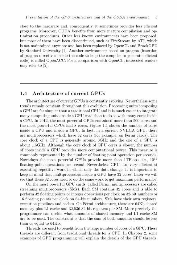
The architecture of current GPUs is constantly evolving. Nevertheless sometrends remain constant throughout this evolution. Processing units composinga GPU are far simpler than a traditional CPU and it is much easier to integratemany computing units inside a GPU card than to do so with many cores insidea CPU. In 2012, the most powerful GPUs contained more than 500 cores andthe most powerful CPUs had 8 cores. Figure 1.1 shows the number of coresinside a CPU and inside a GPU. In fact, in a current NVIDIA GPU, thereare multiprocessors which have 32 cores (for example, on Fermi cards). Thecore clock of a CPU is generally around 3GHz and the one of a GPU isabout 1.5GHz. Although the core clock of GPU cores is slower, the numberof cores inside a GPU provides more computational power. This measure iscommonly represented by the number of floating point operation per seconds.Nowadays the most powerful GPUs provide more than 1TFlops, i.e., 1012
floating point operations per second. Nevertheless GPUs are very efficient atexecuting repetitive work in which only the data change. It is important tokeep in mind that multiprocessors inside a GPU have 32 cores. Later we willsee that these 32 cores need to do the same work to get maximum performance.
On the most powerful GPU cards, called Fermi, multiprocessors are calledstreaming multiprocessors (SMs). Each SM contains 32 cores and is able toperform 32 floating points or integer operations per clock on 32-bit numbers or16 floating points per clock on 64-bit numbers. SMs have their own registers,execution pipelines and caches. On Fermi architecture, there are 64Kb sharedmemory plus L1 cache and 32,536 32-bit registers per SM. More precisely theprogrammer can decide what amounts of shared memory and L1 cache SMare to be used. The constraint is that the sum of both amounts should be lessthan or equal to 64Kb.
Threads are used to benefit from the large number of cores of a GPU. Thesethreads are different from traditional threads for a CPU. In Chapter 2, someexamples of GPU programming will explain the details of the GPU threads.

6 Designing Scientific Applications on GPUs
Core 1 Core 2
CPU GPU
Core 3 Core 4
Core 5 Core 6
Core 7 Core 8
Multiprocessor 1
32 cores
Multiprocessor 3
32 cores
Multiprocessor 2
32 cores
Multiprocessor 4
32 cores
Multiprocessor 15
32 cores
Multiprocessor 16
32 cores
FIGURE 1.1. Comparison of number of cores in a CPU and in a GPU.
Threads are gathered into blocks of 32 threads, called “warps”. These warpsare important when designing an algorithm for GPU.
Another big difference between a CPU and a GPU is the latency of mem-ory. In a CPU, everything is optimized to obtain a low latency architecture.This is possible through the use of cache memories. Moreover, nowadaysCPUs carry out many performance optimizations such as speculative exe-cution which roughly speaking consists of executing a small part of the codein advance even if later this work reveals itself to be useless. GPUs do not havelow latency memory. In comparison GPUs have small cache memories; nev-ertheless the architecture of GPUs is optimized for throughput computationand it takes into account the memory latency.
Figure 1.2 illustrates the main difference of memory latency between aCPU and a GPU. In a CPU, tasks “ti” are executed one by one with a shortmemory latency to get the data to process. After some tasks, there is a contextswitch that allows the CPU to run concurrent applications and/or multi-threaded applications. Memory latencies are longer in a GPU. The principleto obtain a high throughput is to have many tasks to compute. Later we willsee that these tasks are called threads with CUDA. With this principle, assoon as a task is finished the next one is ready to be executed while the waitfor data for the previous task is overlapped by the computation of other tasks.

Presentation of the GPU architecture and of the CUDA environment 7
Processing part Waiting for data Context switching
CPU: optimized for low latency
GPU: optimized for high throughput
Data ready to be processed
t1
t2
t3
t4
t1 t2 t3 t4
ti
FIGURE 1.2. Comparison of low latency of a CPU and high throughput of aGPU.
1.5 Kinds of parallelism
Many kinds of parallelism are available according to the type of hardware.Roughly speaking, there are three classes of parallelism: instruction-level par-allelism, data parallelism, and task parallelism.
Instruction-level parallelism consists in reordering some instructions in or-der to execute some of them in parallel without changing the result of thecode. In modern CPUs, instruction pipelines allow the processor to executeinstructions faster. With a pipeline a processor can execute multiple instruc-tions simultaneously because the output of a task is the input of the nextone.
Data parallelism consists in executing the same program with differentdata on different computing units. Of course, no dependency should existamong the data. For example, it is easy to parallelize loops without depen-dency using the data parallelism paradigm. This paradigm is linked with theSingle Instructions Multiple Data (SIMD) architecture. This is the kind ofparallelism provided by GPUs.
Task parallelism is the common parallelism achieved on clusters and gridsand high performance architectures where different tasks are executed by dif-ferent computing units.

8 Designing Scientific Applications on GPUs
1.6 CUDA multithreading
The data parallelism of CUDA is more precisely based on the Single In-struction Multiple Thread (SIMT) model, because a programmer accesses thecores by the intermediate of threads. In the CUDA model, all cores execute thesame set of instructions but with different data. This model has similaritieswith the vector programming model proposed for vector machines through the1970s and into the 90s, notably the various Cray platforms. On the CUDAarchitecture, the performance is led by the use of a huge number of threads(from thousands up to millions). The particularity of the model is that thereis no context switching as in CPUs and each thread has its own registers. Inpractice, threads are executed by SM and gathered into groups of 32 threads,called warps. Each SM alternatively executes active warps and warps becom-ing temporarily inactive due to waiting of data (as shown in Figure 1.2).
The key to scalability in the CUDA model is the use of a huge number ofthreads. In practice, threads are gathered not only in warps but also in threadblocks. A thread block is executed by only one SM and it cannot migrate. Thetypical size of a thread block is a power of two (for example, 64, 128, 256, or512).
In this case, without changing anything inside a CUDA code, it is possibleto run code with a small CUDA device or the best performing Tesla CUDAcards. Blocks are executed in any order depending on the number of SMsavailable. So the programmer must conceive code having this issue in mind.This independence between thread blocks provides the scalability of CUDAcodes.
A kernel is a function which contains a block of instructions that are ex-ecuted by the threads of a GPU. When the problem considered is a two-dimensional or three-dimensional problem, it is possible to group thread blocksinto a grid. In practice, the number of thread blocks and the size of threadblocks are given as parameters to each kernel. Figure 1.3 illustrates an exam-ple of a kernel composed of 8 thread blocks. Then this kernel is executed on asmall device containing only 2 SMs. So in this case, blocks are executed 2 by2 in any order. If the kernel is executed on a larger CUDA device containing 4SMs, blocks are executed 4 by 4 simultaneously. The execution times shouldbe approximately twice as fast in the latter case. Of course, that dependson other parameters that will be described later (in this chapter and otherchapters).
Thread blocks provide a way to cooperate in the sense that threads ofthe same block cooperatively load and store blocks of memory they all use.Synchronizations of threads in the same block are possible (but not betweenthreads of different blocks). Threads of the same block can also share resultsin order to compute a single result. In Chapter 2, some examples will explainthat.

Presentation of the GPU architecture and of the CUDA environment 9
Block 1 Block 2
Kernel
Block 3 Block 4
Block 5 Block 6
Block 7 Block 8
Block 1 Block 2
Block 3 Block 4
Block 5 Block 6
Block 7 Block 8
SM 1 SM 2
Device
SM 1 SM 2
Device
SM 1 SM 2
Block 1 Block 2 Block 3 Block 4
Block 5 Block 6 Block 7 Block 8
Time
FIGURE 1.3. Scalability of GPU.
1.7 Memory hierarchy
The memory hierarchy of GPUs is different from that of CPUs. In practice,there are registers, local memory, shared memory, cache memory, and globalmemory.
As previously mentioned each thread can access its own registers. It isimportant to keep in mind that the number of registers per block is limited.On recent cards, this number is limited to 64Kb per SM. Access to registersis very fast, so it is a good idea to use them whenever possible.
Likewise each thread can access local memory which, in practice, is muchslower than registers. Local memory is automatically used by the compilerwhen all the registers are occupied, so the best idea is to optimize the use ofregisters even if this involves reducing the number of threads per block.
Shared memory allows cooperation between threads of the same block.This kind of memory is fast but it needs to be manipulated manually and itssize is limited. It is accessible during the execution of a kernel. So the idea

10 Designing Scientific Applications on GPUs
is to fill the shared memory at the start of the kernel with global data thatare used very frequently, then threads can access it for their computation.Threads can obviously change the content of this shared memory either withcomputation or by loading other data and they can store its content in theglobal memory. So shared memory can be seen as a cache memory, which ismanually managed. This obviously requires effort from the programmer.
On recent cards, the programmer may decide what amount of cache mem-ory and shared memory is attributed to a kernel. The cache memory is anL1 cache which is directly managed by the GPU. Sometimes, this cache pro-vides very efficient result and sometimes the use of shared memory is a bettersolution.
Figure 1.4 illustrates the memory hierarchy of a GPU. Threads are repre-sented on the top of the figure. They can have access to their own registers andtheir local memory. Threads of the same block can access the shared memoryof that block. The cache memory is not represented here but it is local to athread. Then each block can access the global memory of the GPU.
Registe
rs
Registe
rs
Registe
rs
Registe
rs
Registe
rs
Registe
rs
Registe
rs
Registe
rs
Loca
l var
Loca
l var
Loca
l var
Loca
l var
Loca
l var
Loca
l var
Loca
l var
Loca
l var
Shared memory
Registe
rs
Registe
rs
Registe
rs
Registe
rs
Registe
rs
Registe
rs
Registe
rs
Registe
rs
Loca
l var
Loca
l var
Loca
l var
Loca
l var
Loca
l var
Loca
l var
Loca
l var
Loca
l var
Shared memory
Registe
rs
Registe
rs
Registe
rs
Registe
rs
Registe
rs
Registe
rs
Registe
rs
Registe
rs
Loca
l var
Loca
l var
Loca
l var
Loca
l var
Loca
l var
Loca
l var
Loca
l var
Loca
l var
Shared memory
Global memoryFIGURE 1.4. Memory hierarchy of a GPU.

Presentation of the GPU architecture and of the CUDA environment 11
1.8 Conclusion
In this chapter, a brief presentation of the video card, which has later beenused to perform computation, has been given. The architecture of a GPU hasbeen illustrated focusing on the particularity of GPUs in terms of parallelism,memory latency, and threads. In order to design an efficient algorithm forGPU, it is essential to keep all these parameters in mind.
Bibliography
[1] I. Buck, T. Foley, D. Horn, J. Sugerman, K. Fatahalian, M. Houston, andP. Hanrahan. Brook for GPUs: stream computing on graphics hardware.ACM Transactions on Graphics, 23(3):777–786, August 2004.
[2] P. Dua, R. Webera, P. Luszczeka, S. Tomova, G. Petersona, and J. Don-garra. From CUDA to OpenCL: Towards a performance-portable solutionfor multi-platform GPU programming. Parallel Computing, 38(8):391–407,2012.
[3] NVIDIA Corporation. NVIDIA CUDA C Programming Guide, 2011. Ver-sion 4.0.

This page intentionally left blankThis page intentionally left blank

Chapter 2
Introduction to CUDA
Raphael Couturier
Femto-ST Institute, University of Franche-Comte, France
2.1 Introduction . . . . . . . . . . . . . . . . . . . . . . . . . . . . . . . . . . . . . . . . . . . . . . . . . . . . . . 132.2 First example . . . . . . . . . . . . . . . . . . . . . . . . . . . . . . . . . . . . . . . . . . . . . . . . . . . . 132.3 Second example: using CUBLAS . . . . . . . . . . . . . . . . . . . . . . . . . . . . . . . . 162.4 Third example: matrix-matrix multiplication . . . . . . . . . . . . . . . . . . . 182.5 Conclusion . . . . . . . . . . . . . . . . . . . . . . . . . . . . . . . . . . . . . . . . . . . . . . . . . . . . . . . . 21
Bibliography . . . . . . . . . . . . . . . . . . . . . . . . . . . . . . . . . . . . . . . . . . . . . . . . . . . . . . 21
2.1 Introduction
In this chapter we give some simple examples of CUDA programming. Thegoal is not to provide an exhaustive presentation of all the functionalities ofCUDA but rather to give some basic elements. Of course, readers who do notknow CUDA are invited to read other books that are specialized on CUDAprogramming (for example, [2]).
2.2 First example
This first example is intented to show how to build a very simple programwith CUDA. Its goal is to perform the sum of two arrays and put the resultinto a third array. A CUDA program consists in a C code which calls CUDAkernels that are executed on a GPU. This code is in Listing 2.1.
As GPUs have their own memory, the first step consists of allocating mem-ory on the GPU. A call to cudaMalloc allocates memory on the GPU. Thefirst parameter of this function is a pointer on a memory on the device, i.e.,the GPU. The second parameter represents the size of the allocated variables;this size is expressed in bits.
13

14 Designing Scientific Applications on GPUs
Listing 2.1. simple example
#include <s t d l i b . h>#include <s t d i o . h>#include <s t r i n g . h>#include <math . h>
5 #include <a s s e r t . h>#include "cutil_inline.h"
const int nbThreadsPerBloc =256;
10 g l o b a lvoid add i t i on ( int s i z e , int ∗d C , int ∗d A , int ∗d B )
int t i d = blockIdx . x ∗ blockDim . x + threadIdx . x ;i f ( t id<s i z e )
d C [ t i d ]=d A [ t i d ]+d B [ t i d ] ;15
int main ( int argc , char∗∗ argv )20
i f ( argc !=2) p r i n t f ("usage: ex1 nb_components\n" ) ;e x i t (0 ) ;
25
int s i z e=a t o i ( argv [ 1 ] ) ;int i ;int ∗h arrayA=( int ∗) mal loc ( s i z e ∗ s izeof ( int ) ) ;int ∗h arrayB=( int ∗) mal loc ( s i z e ∗ s izeof ( int ) ) ;
30 int ∗h arrayC=( int ∗) mal loc ( s i z e ∗ s izeof ( int ) ) ;int ∗h arrayCgpu=( int ∗) mal loc ( s i z e ∗ s izeof ( int ) ) ;int ∗d arrayA , ∗d arrayB , ∗d arrayC ;
cudaMalloc ( ( void ∗∗)&d arrayA , s i z e ∗ s izeof ( int ) ) ;35 cudaMalloc ( ( void ∗∗)&d arrayB , s i z e ∗ s izeof ( int ) ) ;
cudaMalloc ( ( void ∗∗)&d arrayC , s i z e ∗ s izeof ( int ) ) ;
for ( i =0; i<s i z e ; i++) h arrayA [ i ]= i ;
40 h arrayB [ i ]=2∗ i ;
unsigned int t imer cpu = 0 ;cut i lCheckError ( cutCreateTimer(&timer cpu ) ) ;
45 cut i lCheckError ( cutStartTimer ( t imer cpu ) ) ;for ( i =0; i<s i z e ; i++)
h arrayC [ i ]=h arrayA [ i ]+ h arrayB [ i ] ;cut i lCheckError ( cutStopTimer ( t imer cpu ) ) ;
50 p r i n t f ("CPU processing time : %f (ms) \n" , cutGetTimerValue (t imer cpu ) ) ;
cutDeleteTimer ( t imer cpu ) ;
unsigned int t imer gpu = 0 ;cut i lCheckError ( cutCreateTimer(&timer gpu ) ) ;
55 cut i lCheckError ( cutStartTimer ( t imer gpu ) ) ;cudaMemcpy( d arrayA , h arrayA , s i z e ∗ s izeof ( int ) ,
cudaMemcpyHostToDevice ) ;cudaMemcpy( d arrayB , h arrayB , s i z e ∗ s izeof ( int ) ,
cudaMemcpyHostToDevice ) ;
int nbBlocs=( s i z e+nbThreadsPerBloc−1)/nbThreadsPerBloc ;60 addit ion<<<nbBlocs , nbThreadsPerBloc>>>(s i z e , d arrayC , d arrayA ,
d arrayB ) ;

Introduction to CUDA 15
cudaMemcpy( h arrayCgpu , d arrayC , s i z e ∗ s izeof ( int ) ,cudaMemcpyDeviceToHost ) ;
cut i lCheckError ( cutStopTimer ( t imer gpu ) ) ;p r i n t f ("GPU processing time : %f (ms) \n" , cutGetTimerValue (
t imer gpu ) ) ;65 cutDeleteTimer ( t imer gpu ) ;
for ( i =0; i<s i z e ; i++) a s s e r t ( h arrayC [ i ]==h arrayCgpu [ i ] ) ;
70 cudaFree ( d arrayA ) ;
cudaFree ( d arrayB ) ;cudaFree ( d arrayC ) ;f r e e ( h arrayA ) ;f r e e ( h arrayB ) ;
75 f r e e ( h arrayC ) ;return 0 ;
In this example, we want to compare the execution time of the additions oftwo arrays in CPU and GPU. So for both these operations, a timer is createdto measure the time. CUDA manipulates timers quite easily. The first step isto create the timer, then to start it, and at the end to stop it. For each ofthese operations a dedicated function is used.
In order to compute the same sum with a GPU, the first step consistsof transferring the data from the CPU (considered as the host with CUDA)to the GPU (considered as the device with CUDA). A call to cudaMemcpycopies the content of an array allocated in the host to the device when thefourth parameter is set to cudaMemcpyHostToDevice. The first parameterof the function is the destination array, the second is the source array, and thethird is the number of elements to copy (expressed in bytes).
Now the GPU contains the data needed to perform the addition. In sequen-tial programming, such addition is achieved with a loop on all the elements.With a GPU, it is possible to perform the addition of all the elements of thetwo arrays in parallel (if the number of blocks and threads per blocks is suf-ficient). In Listing 2.1 at the beginning, a simple kernel, called addition isdefined to compute in parallel the summation of the two arrays. With CUDA,a kernel starts with the keyword global which indicates that this kernelcan be called from the C code. The first instruction in this kernel is used tocompute the variable tid which represents the thread index. This thread in-dex is computed according to the values of the block index (called blockIdxin CUDA) and of the thread index (called threadIdx in CUDA). Blocksof threads and thread indexes can be decomposed into 1 dimension, 2 di-mensions, or 3 dimensions. According to the dimension of manipulated data,the dimension of blocks of threads must be chosen carefully. In our example,only one dimension is used. Then using the notation .x, we can access thefirst dimension (.y and .z, respectively allow access to the second and thirddimensions). The variable blockDim gives the size of each block.

16 Designing Scientific Applications on GPUs
2.3 Second example: using CUBLAS
The Basic Linear Algebra Subprograms (BLAS) allow programmers to useefficient routines for basic linear operations. Those routines are heavily used inmany scientific applications and are optimized for vector operations, matrix-vector operations, and matrix-matrix operations [1]. Some of those operationsseem to be easy to implement with CUDA; however, as soon as a reductionis needed, implementing an efficient reduction routine with CUDA is far frombeing simple. Roughly speaking, a reduction operation is an operation whichcombines all the elements of an array and extracts a number computed from allthe elements. For example, a sum, a maximum, or a dot product are reductionoperations.
In this second example, we have two vectors A and B. First of all, we wantto compute the sum of both vectors and store the result in a vector C. Thenwe want to compute the scalar product between 1/C and 1/A. This is just anexample which has no direct interest except to show how to program it withCUDA.
Listing 2.2 shows this example with CUDA. The first kernel for the additionof two arrays is exactly the same as the one described in the previous example.
The kernel to compute the inverse of the elements of an array is verysimple. For each thread index, the inverse of the array replaces the initialarray.
In the main function, the beginning is very similar to the one in the previ-ous example. First, the user is asked to define the number of elements. Thena call to cublasCreate initializes the CUBLAS library. It creates a han-dle. Then all the arrays are allocated in the host and the device, as in theprevious example. Both arrays A and B are initialized. The CPU computa-tion is performed and the time for this is measured. In order to compute thesame result for the GPU, first of all, data from the CPU need to be copiedinto the memory of the GPU. For that, it is possible to use CUBLAS functioncublasSetVector. This function has several arguments. More precisely, thefirst argument represents the number of elements to transfer, the second argu-ments is the size of each element, the third element represents the source of thearray to transfer (in the GPU), the fourth is an offset between each elementof the source (usually this value is set to 1), the fifth is the destination (inthe GPU), and the last is an offset between each element of the destination.Then we call the kernel addition which computes the sum of all elements ofarrays A and B. The inverse kernel is called twice, once to inverse elementsof array C and once for A. Finally, we call the function cublasDdot whichcomputes the dot product of two vectors. To use this routine, we must specifythe handle initialized by CUDA, the number of elements to consider, theneach vector is followed by the offset between every element. After the GPU

Introduction to CUDA 17
computation, it is possible to check that both computations produce the sameresult.
Listing 2.2. simple example with CUBLAS
#include <s t d l i b . h>#include <s t d i o . h>#include <s t r i n g . h>#include <math . h>
5 #include <a s s e r t . h>#include "cutil_inline.h"#include <cub las v2 . h>
const int nbThreadsPerBloc =256;10
g l o b a lvoid add i t i on ( int s i z e , double ∗d C , double ∗d A , double ∗d B )
int t i d = blockIdx . x ∗ blockDim . x + threadIdx . x ;i f ( t id<s i z e )
15 d C [ t i d ]=d A [ t i d ]+d B [ t i d ] ;
g l o b a l20 void i n v e r s e ( int s i z e , double ∗d x )
int t i d = blockIdx . x ∗ blockDim . x + threadIdx . x ;i f ( t id<s i z e )
d x [ t i d ]=1./ d x [ t i d ] ;
25
int main ( int argc , char∗∗ argv )
30 i f ( argc !=2) p r i n t f ("usage: ex2 nb_components\n" ) ;e x i t (0 ) ;
35 int s i z e=a t o i ( argv [ 1 ] ) ;cub l a sS t a tu s t s t a t ;cub lasHandle t handle ;s t a t=cublasCreate (&handle ) ;int i ;
40 double ∗h arrayA=(double∗) mal loc ( s i z e ∗ s izeof (double ) ) ;double ∗h arrayB=(double∗) mal loc ( s i z e ∗ s izeof (double ) ) ;double ∗h arrayC=(double∗) mal loc ( s i z e ∗ s izeof (double ) ) ;double ∗h arrayCgpu=(double∗) mal loc ( s i z e ∗ s izeof (double ) ) ;double ∗d arrayA , ∗d arrayB , ∗d arrayC ;
45
cudaMalloc ( ( void ∗∗)&d arrayA , s i z e ∗ s izeof (double ) ) ;cudaMalloc ( ( void ∗∗)&d arrayB , s i z e ∗ s izeof (double ) ) ;cudaMalloc ( ( void ∗∗)&d arrayC , s i z e ∗ s izeof (double ) ) ;
50 for ( i =0; i<s i z e ; i++) h arrayA [ i ]= i +1;h arrayB [ i ]=2∗( i +1) ;
55 unsigned int t imer cpu = 0 ;cut i lCheckError ( cutCreateTimer(&timer cpu ) ) ;cut i lCheckError ( cutStartTimer ( t imer cpu ) ) ;double dot =0;for ( i =0; i<s i z e ; i++)
60 h arrayC [ i ]=h arrayA [ i ]+ h arrayB [ i ] ;dot +=(1./ h arrayC [ i ] ) ∗ ( 1 . / h arrayA [ i ] ) ;

18 Designing Scientific Applications on GPUs
cut i lCheckError ( cutStopTimer ( t imer cpu ) ) ;p r i n t f ("CPU processing time : %f (ms) \n" , cutGetTimerValue (
t imer cpu ) ) ;65 cutDeleteTimer ( t imer cpu ) ;
unsigned int t imer gpu = 0 ;cut i lCheckError ( cutCreateTimer(&timer gpu ) ) ;cut i lCheckError ( cutStartTimer ( t imer gpu ) ) ;
70 s t a t = cublasSetVector ( s i z e , s izeof (double ) , h arrayA , 1 , d arrayA , 1 ) ;s t a t = cublasSetVector ( s i z e , s izeof (double ) , h arrayB , 1 , d arrayB , 1 ) ;int nbBlocs=( s i z e+nbThreadsPerBloc−1)/nbThreadsPerBloc ;
addit ion<<<nbBlocs , nbThreadsPerBloc>>>(s i z e , d arrayC , d arrayA ,d arrayB ) ;
75 i nve r se<<<nbBlocs , nbThreadsPerBloc>>>(s i z e , d arrayC ) ;inver se<<<nbBlocs , nbThreadsPerBloc>>>(s i z e , d arrayA ) ;double dot gpu =0;s t a t = cublasDdot ( handle , s i z e , d arrayC , 1 , d arrayA ,1 ,& dot gpu ) ;
80 cut i lCheckError ( cutStopTimer ( t imer gpu ) ) ;p r i n t f ("GPU processing time : %f (ms) \n" , cutGetTimerValue (
t imer gpu ) ) ;cutDeleteTimer ( t imer gpu ) ;p r i n t f ("cpu dot %e --- gpu dot %e\n" , dot , dot gpu ) ;
85 cudaFree ( d arrayA ) ;cudaFree ( d arrayB ) ;cudaFree ( d arrayC ) ;f r e e ( h arrayA ) ;f r e e ( h arrayB ) ;
90 f r e e ( h arrayC ) ;f r e e ( h arrayCgpu ) ;cublasDestroy ( handle ) ;return 0 ;
2.4 Third example: matrix-matrix multiplication
Matrix-matrix multiplication is an operation which is quite easy to paral-lelize with a GPU. If we consider that a matrix is represented using a two-dimensional array, A[i][j] represents the element of the i row and of the jcolumn. In many cases, it is easier to manipulate a one-dimentional (1D) ar-ray rather than a 2D array. With CUDA, even if it is possible to manipulate2D arrays, in the following we present an example based on a 1D array. Forthe sake of simplicity, we consider we have a square matrix of size size. Sowith a 1D array, A[i*size+j] allows us to have access to the element of thei row and of the j column.
With sequential programming, the matrix-matrix multiplication is per-formed using three loops. We assume that A, B represent two square matricesand the result of the multiplication of A×B is C. The element C[i*size+j]

Introduction to CUDA 19
is computed as follows:
C[size ∗ i+ j] =
size−1∑k=0
A[size ∗ i+ k] ∗B[size ∗ k + j]. (2.1)
In Listing 2.3, the CPU computation is performed using 3 loops, one fori, one for j, and one for k. In order to perform the same computation on aGPU, a naive solution consists of considering that the matrix C is split into2-dimensional blocks. The size of each block must be chosen such that thenumber of threads per block is less than 1, 024.
In Listing 2.3, we consider that a block contains 16 threads in each dimen-sion, the variable width is used for that. The variable nbTh represents thenumber of threads per block. So, to compute the matrix-matrix product on aGPU, each block of threads is assigned to compute the result of the productof the elements of that block. The main part of the code is quite similar to theprevious code. Arrays are allocated in the CPU and the GPU. Matrices A andB are randomly initialized. Then arrays are transferred to the GPU memorywith call to cudaMemcpy. So the first step for each thread of a block is tocompute the corresponding row and column. With a 2-dimensional decompo-sition, int i= blockIdx.y*blockDim.y+ threadIdx.y; allows us tocompute the corresponding line and int j= blockIdx.x*blockDim.x+threadIdx.x; the corresponding column. Then each thread has to com-pute the sum of the product of the row of A by the column of B. In order touse a register, the kernel matmul uses a variable called sum to compute thesum. Then the result is set into the matrix at the right place. The compu-tation of CPU matrix-matrix multiplication is performed as described previ-ously. A timer measures the time. In order to use 2-dimensional blocks, dim3dimGrid(size/width,size/width); allows us to create size/widthblocks in each dimension. Likewise, dim3 dimBlock(width,width); isused to create width thread in each dimension. After that, the kernel for thematrix multiplication is called. At the end of the listing, the matrix C com-puted by the GPU is transferred back into the CPU and we check that bothmatrices C computed by the CPU and the GPU are identical with a precisionof 10−4.
With 1, 024 × 1, 024 matrices, on a C2070M Tesla card, this code takes37.68ms to perform the multiplication. With an Intel Xeon E31245 at3.30GHz, it takes 2465ms without any parallelization (using only one core).Consequently the speed up between the CPU and GPU version is about 65which is very good considering the difficulty of parallelizing this code.
Listing 2.3. simple matrix-matrix multiplication with cuda
#include <s t d l i b . h>#include <s t d i o . h>#include <s t r i n g . h>#include <math . h>
5 #include <a s s e r t . h>#include "cutil_inline.h"

20 Designing Scientific Applications on GPUs
#include <cub las v2 . h>
const int width =16;10 const int nbTh=width∗width ;
const int s i z e =1024;const int s izeMat=s i z e ∗ s i z e ;
15 g l o b a lvoid matmul ( f loat ∗d A , f loat ∗d B , f loat ∗d C )
int i= blockIdx . y∗blockDim . y+ threadIdx . y ;int j= blockIdx . x∗blockDim . x+ threadIdx . x ;
20 f loat sum=0;for ( int k=0;k<s i z e ; k++)
sum+=d A [ i ∗ s i z e+k ]∗ d B [ k∗ s i z e+j ] ;d C [ i ∗ s i z e+j ]=sum ;
25
int main ( int argc , char∗∗ argv )
f loat ∗h arrayA=( f loat ∗) mal loc ( s izeMat ∗ s izeof ( f loat ) ) ;30 f loat ∗h arrayB=( f loat ∗) mal loc ( s izeMat ∗ s izeof ( f loat ) ) ;
f loat ∗h arrayC=( f loat ∗) mal loc ( s izeMat ∗ s izeof ( f loat ) ) ;f loat ∗h arrayCgpu=( f loat ∗) mal loc ( s izeMat ∗ s izeof ( f loat ) ) ;
f loat ∗d arrayA , ∗d arrayB , ∗d arrayC ;35
cudaMalloc ( ( void ∗∗)&d arrayA , sizeMat ∗ s izeof ( f loat ) ) ;cudaMalloc ( ( void ∗∗)&d arrayB , sizeMat ∗ s izeof ( f loat ) ) ;cudaMalloc ( ( void ∗∗)&d arrayC , sizeMat ∗ s izeof ( f loat ) ) ;
40 srand48 (32) ;for ( int i =0; i<s izeMat ; i++)
h arrayA [ i ]=drand48 ( ) ;h arrayB [ i ]=drand48 ( ) ;h arrayC [ i ]=0;
45 h arrayCgpu [ i ]=0;
cudaMemcpy( d arrayA , h arrayA , sizeMat ∗ s izeof ( f loat ) ,cudaMemcpyHostToDevice ) ;
50 cudaMemcpy( d arrayB , h arrayB , sizeMat ∗ s izeof ( f loat ) ,cudaMemcpyHostToDevice ) ;
cudaMemcpy( d arrayC , h arrayC , sizeMat ∗ s izeof ( f loat ) ,cudaMemcpyHostToDevice ) ;
unsigned int t imer cpu = 0 ;cut i lCheckError ( cutCreateTimer(&timer cpu ) ) ;
55 cut i lCheckError ( cutStartTimer ( t imer cpu ) ) ;int sum=0;for ( int i =0; i<s i z e ; i++)
for ( int j =0; j<s i z e ; j++) for ( int k=0;k<s i z e ; k++)
60 h arrayC [ s i z e ∗ i+j ]+=h arrayA [ s i z e ∗ i+k ]∗ h arrayB [ s i z e ∗k+j ] ;
cut i lCheckError ( cutStopTimer ( t imer cpu ) ) ;
65 p r i n t f ("CPU processing time : %f (ms) \n" , cutGetTimerValue (t imer cpu ) ) ;
cutDeleteTimer ( t imer cpu ) ;
unsigned int t imer gpu = 0 ;cut i lCheckError ( cutCreateTimer(&timer gpu ) ) ;

Introduction to CUDA 21
70 cut i lCheckError ( cutStartTimer ( t imer gpu ) ) ;
dim3 dimGrid ( s i z e /width , s i z e /width ) ;dim3 dimBlock ( width , width ) ;
75 matmul<<<dimGrid , dimBlock>>>(d arrayA , d arrayB , d arrayC ) ;cudaThreadSynchronize ( ) ;
cut i lCheckError ( cutStopTimer ( t imer gpu ) ) ;p r i n t f ("GPU processing time : %f (ms) \n" , cutGetTimerValue (
t imer gpu ) ) ;80 cutDeleteTimer ( t imer gpu ) ;
cudaMemcpy( h arrayCgpu , d arrayC , sizeMat ∗ s izeof ( f loat ) ,cudaMemcpyDeviceToHost ) ;
for ( int i =0; i<s izeMat ; i++)85 i f ( fabs ( h arrayC [ i ]−h arrayCgpu [ i ] )>1e−4)
p r i n t f ("%f %f\n" , h arrayC [ i ] , h arrayCgpu [ i ] ) ;
cudaFree ( d arrayA ) ;cudaFree ( d arrayB ) ;
90 cudaFree ( d arrayC ) ;f r e e ( h arrayA ) ;f r e e ( h arrayB ) ;f r e e ( h arrayC ) ;f r e e ( h arrayCgpu ) ;
95 return 0 ;
2.5 Conclusion
In this chapter, three simple CUDA examples have been presented. Aswe cannot present all the possibilities of the CUDA programming, interestedreaders are invited to consult CUDA programming introduction books if someissues regarding the CUDA programming are not clear.
Bibliography
[1] J. Dongarra. Basic linear algebra subprograms technical (BLAST) forumstandard (1). International Journal of High Performance Computing Ap-plications, 16(1):1–111, 2002.
[2] J. Sanders and E. Kandrot. CUDA by example: An Introduction ToGeneral-Purpose GPU Programming. Addison-Wesley, Upper SaddleRiver, NJ, 2010.

This page intentionally left blankThis page intentionally left blank

Part II
Image processing

This page intentionally left blankThis page intentionally left blank

Chapter 3
Setting up the environment
Gilles Perrot
Femto-ST Institute, University of Franche-Comte, France
3.1 Data transfers, memory management . . . . . . . . . . . . . . . . . . . . . . . . . . . . 253.2 Performance measurements . . . . . . . . . . . . . . . . . . . . . . . . . . . . . . . . . . . . . . 28
Image processing using a GPU often means using it as a general purpose com-puting processor, which soon brings up the issue of data transfers, especiallywhen kernel runtime is fast and/or when large data sets are processed. Thetruth is that, in certain cases, data transfers between GPU and CPU are slowerthan the actual computation on GPU. It remains that global runtime can stillbe faster than similar processes run on CPU. Therefore, to fully optimizeglobal runtimes, it is important to pay attention to how memory transfersare done. This leads us to propose, in the following section, an overall codestructure to be used with all our kernel examples.
Obviously, our code originally accepts various image dimensions and canprocess color images when an extrapolated definition of the median filter ischoosen. However, so as to propose concise and more readable code, we willassume the following limitations: 16 bit-coded gray-level input images whosedimensions H ×W are multiples of 512 pixels.
3.1 Data transfers, memory management
This section deals with the following issues:
1. Data transfer from CPU memory to GPU global memory: several GPUmemory areas are available as destination memory but the 2D cachingmechanism of texture memory, specifically designed for fetching neigh-boring pixels, is currently the fastest way to fetch gray-level pixel valuesinside a kernel computation. This has led us to choose texture memoryas primary GPU memory area for input images.
2. Data fetching from GPU global memory to kernel local memory: as
25

26 Designing Scientific Applications on GPUs
said above, we use texture memory. Depending on which process is run,texture data is used either by direct fetching in kernel local memory orthrough a prefetching in shared memory.
3. Data outputting from kernels to GPU memory: there is actually no al-ternative to global memory, as kernels cannot directly write into texturememory and as copying from texture to CPU memory would not befaster than from simple global memory.
4. Data transfer from GPU global memory to CPU memory: it can bedrastically accelerated by use of pinned memory, keeping in mind ithas to be used sparingly.
Algorithm 1 summarizes all the above considerations and describes how dataare handled in our examples. For more information on how to handle the dif-ferent types of GPU memory, we suggest referring to the CUDA programmer’sguide.
Algorithm 1: global memory management on CPU and GPU sides
1 allocate and populate CPU memory h in;2 allocate CPU pinned-memory h out;3 allocate GPU global memory d out;4 declare GPU texture reference tex img in;5 allocate GPU array in global memory array img in;6 bind GPU array array img in to texture tex img in;7 copy data from h in to array img in;8 kernel gridDim,blockDim () /* outputs to d out */;9 copy data from d out to h out ;
At debug stage, for simplicity’s sake, we use the cutil library suppliedby the NVIDIA software development kit (SDK). Thus, in order to eas-ily implement our examples, we suggest readers download and install thelatest NVIDIA-SDK (ours is SDK4.0), create a new directory SDK-root-dir/C/src/fast kernels and adapt the generic Makefile that can be found ineach subdirectory of SDK-root-dir/C/src/. Then, only two more files will beneeded to have a fully operational environnement: main.cu and fast kernels.cu.Listings 3.1, 3.2 and 3.3 implement all the above considerations minimally,while remaining functional.
The main file of Listing 3.1 is a simplified version of our actual main file.It has to be noted that functions cutLoadPGMi and cutSavePGMi of thecutil library operate only on unsigned integer data. As data is coded in shortinteger format for performance reasons, the use of these functions involves onedata cast after loading and before saving. This may be overcome by use of adifferent library. Actually, our choice was to modify the above mentioned cutilfunctions.

Setting up the environment 27
Listing 3.2 gives a minimal kernel skeleton that will serve as the basis forall other kernels. Lines 5 and 6 determine the coordinates (i, j) of the pixelto be processed, each pixel being associated to one thread. The instruction inline 8 combines writing the output gray-level value into global memory andfetching the input gray-level value from 2D texture memory. The Makefilegiven in Listing 3.3 shows how to adapt examples given in SDK.
Listing 3.1. generic main.cu file used to launch CUDA kernels
#include <cuda runtime . h>#include <c u t i l i n l i n e . h>#include "fast_kernels.cu"
5 int main ( int argc , char ∗∗ argv )cudaSetDevice ( 0 ) ; // select f i r s t GPUchar f i l ename [ 8 0 ] = "image.pgm" ;short ∗ h in , ∗h out , ∗ d out ;int s i z e , bsx=16, bsy=16 ;
10 dim3 dimBlock , dimGrid ;cudaChannelFormatDesc channelD=cudaCreateChannelDesc<short>() ;cudaArray ∗ ar ray img in ;/∗ . . . . . . . . . . . . . . . . . . . . . . . load image and cast . . . . . . . . . . . ∗/unsigned int ∗ h img = NULL ;
15 unsigned int ∗ h outui , H, L ;cut i lCheckError ( cutLoadPGMi( f i l ename , &h img , &L , &H) ) ;s i z e = H ∗ L ∗ s izeof ( short ) ;h in = new short [H∗L ] ;for ( int k=0; k<H∗L ; k++)
20 h in [ k ] = ( short ) h img [ k ] ;/∗ . . . . . . . . . . . . . . . . . . . . . . . end of image load . . . . . . . . . . . . . ∗/cudaHostAlloc ( ( void ∗∗)&h out , s i z e , cudaHostAl locDefault ) ;cudaMalloc ( ( void ∗∗) &d out , s i z e ) ;cudaMallocArray ( &array img in , &channelD , W, H ) ;
25 cudaBindTextureToArray ( tex img in , ar ray img in , channelD ) ;cudaMemcpyToArray ( array img in , 0 , 0 , h in , s i z e ,
cudaMemcpyHostToDevice ) ;dimBlock = dim3 ( bsx , bsy , 1 ) ;dimGrid = dim3 ( L/dimBlock . x , H/dimBlock . y , 1) ;
30 k e r n e l t e s t<<< dimGrid , dimBlock , 0>>>(d out , W, H) ;
c u t i l S a f e C a l l ( cudaMemcpy( h out , d out , s i z e ,cudaMemcpyDeviceToHost ) ) ;
/∗ . . . . . . . . . . . . . . . cast and save output image ( optional ) ∗/h outu i = new unsigned int [H∗L ] ;
35 for ( int k=0; k<H∗L ; k++)h outu i [ k ] = (unsigned int ) h out [ k ] ;
cut i lCheckError ( cutSavePGMi ("image_out.pgm" , h outui , L , H) ) ;
cudaFreeHost ( h out ) ;40 cudaFree ( d out ) ;
return 0 ;
Listing 3.2. fast kernels.cu file featuring one kernel skeleton
texture<short , 2 , cudaReadModeElementType> t ex img in ;
g l o b a l void k e r n e l i d e n t ( short ∗output , int w)
5 int j = mul24 ( blockIdx . x , blockDim . x ) + threadIdx . x ;int i = mul24 ( blockIdx . y , blockDim . y ) + threadIdx . y ;

28 Designing Scientific Applications on GPUs
output [ mul24 ( i , w) + j ] = tex2D ( tex img in , j , i ) ;
10
Listing 3.3. generic makefile based on those provided by NVIDIA SDK
EXECUTABLE := fast medianCUFILES := main . cu
inc lude . . / . . / common/common .mk5
NVCCFLAGS += −arch=sm 20NVCCFLAGS += −−ptxas−opt ions=−v
3.2 Performance measurements
As our goal is to design very fast implementations of basic image processingalgorithms, we need to make quite accurate time-measurements, within theorder of magnitude of 0.01 ms. Again, the easiest way of doing so is to use thehelper functions of the cutil library. As usual, because the durations we aremeasuring are short and possibly subject to nonnegligible variations, a goodpractice is to measure multiple executions and report the mean runtime. Alltime results given in this chapter have been obtained through 1000 calls toeach kernel.
Listing 3.4 shows how to use the dedicated cutil functions. Timer dec-laration and creation need to be performed only once while reset, start andstop functions can be used as often as necessary. Synchronization is manda-tory before stopping the timer (Line 7), to avoid runtime measurement beingbiased.
Listing 3.4. Time measurement technique using cutil functions
unsigned int t imer ;cut i lCheckError ( cutCreateTimer(&timer ) ) ;cut i lCheckError ( cutResetTimer ( t imer ) ) ;cut i lCheckError ( cutStartTimer ( t imer ) ) ;
5 for ( int ct =0; ct<1000 ; ct++)ke rne l i d en t<<< dimGrid , dimBlock , 0>>>(d out , W) ;
cudaThreadSynchronize ( ) ;cut i lCheckError ( cutStopTimer ( t imer ) ) ;cut i lCheckError ( cutStopTimer ( t imer ) ) ;
10 p r i n t f ("Mean runtime: %f ms,\n" , cutGetTimerValue ( t imer ) /1000) ;
In an attempt to provide relevant speedup values, we either implementedCPU versions of the algorithms studied or used the values found in existingliterature. Still, the large number and diversity of hardware platforms andGPU cards makes it impossible to benchmark every possible combination andsignificant differences may occur between the speedups we report and those

Setting up the environment 29
obtained with different devices. As a reference, our developing platform detailsas follows:
• CPU codes run on
– Xeon: a recent and very efficient Quad Core Xeon E31245 at3.3GHz-8GByte RAM running Linux kernel 3.2.
• GPU codes run on
– C2070: NVIDIA Tesla C2070 hosted by a PC QuadCore XeonE5620 at 2.4GHz-12GByte RAM, running Linux kernel 2.6.18
– GTX280: NVIDIA GeForce GTX 280 hosted by a PC QuadCoreXeon X5482 at 3.20GHz-4GByte RAM, running Linux kernel 2.6.32
All kernels have also been tested with various image sizes from 512×512to 4096×4096 pixels. This allows estimating runtime dependancy over imagesize.
Last, like many authors, we chose to use the pixel throughput value of eachprocess in Mega Pixels per second (MP/s) as a performance indicator, includ-ing data transfers and kernel runtimes. In order to estimate the potential forimprovement of each kernel, a reference throughput measurement, involvingthe identity kernel of Listing 3.2, was performed. As this kernel only fetchesinput values from texture memory and outputs them to global memory with-out doing any computation, it represents the smallest, thus fastest, possibleprocess and is taken as the reference throughput value (100%). The same mea-surement was performed on CPU, with a maximum effective pixel throughputof 130 MP/s. On GPU, depending on grid parameters this measurement was800 MP/s on GTX280 and 1300 MP/s on C2070.

This page intentionally left blankThis page intentionally left blank

Chapter 4
Implementing a fast median filter
Gilles Perrot
Femto-ST Institute, University of Franche-Comte, France
4.1 Introduction . . . . . . . . . . . . . . . . . . . . . . . . . . . . . . . . . . . . . . . . . . . . . . . . . . . . . . 314.2 Median filtering . . . . . . . . . . . . . . . . . . . . . . . . . . . . . . . . . . . . . . . . . . . . . . . . . . 32
4.2.1 Basic principles . . . . . . . . . . . . . . . . . . . . . . . . . . . . . . . . . . . . . . . . . . 324.2.2 A naive implementation . . . . . . . . . . . . . . . . . . . . . . . . . . . . . . . . . 33
4.3 NVIDIA GPU tuning recipes . . . . . . . . . . . . . . . . . . . . . . . . . . . . . . . . . . . . 354.4 A 3×3 median filter: using registers . . . . . . . . . . . . . . . . . . . . . . . . . . . . . 37
4.4.1 The simplest way . . . . . . . . . . . . . . . . . . . . . . . . . . . . . . . . . . . . . . . . 374.4.2 Further optimization . . . . . . . . . . . . . . . . . . . . . . . . . . . . . . . . . . . . 38
4.4.2.1 Reducing register count . . . . . . . . . . . . . . . . . . . 394.4.2.2 More data output per thread . . . . . . . . . . . . . . 42
4.5 A 5×5 and more median filter . . . . . . . . . . . . . . . . . . . . . . . . . . . . . . . . . . 444.5.1 A register-only 5×5 median filter . . . . . . . . . . . . . . . . . . . . . . . 444.5.2 Fast approximated n× n median filter . . . . . . . . . . . . . . . . . 47Bibliography . . . . . . . . . . . . . . . . . . . . . . . . . . . . . . . . . . . . . . . . . . . . . . . . . . . . . . 51
4.1 Introduction
Median filtering is a well-known method used in a wide range of applica-tion frameworks as well as a standalone filter especially for salt and pepperdenoising. It is able to greatly reduce the power of noise without blurringedges too much. That is actually why we originally focused on this filteringtechnique as a preprocessing stage when we were in the process of designing aGPU implementation of one region-based image segmentation algorithm [8].
First introduced by Tukey in [10], it has been widely studied since then,and many researchers have proposed efficient implementations of it, adaptedto various hypotheses, architectures and processors. Originally, its main draw-backs were its compute complexity, its nonlinearity and its data-dependentruntime. Several researchers have addressed these issues and designed, forexample, efficient histogram-based median filters with predictible runtimes[3, 11].
More recently, the advent of GPUs opened new perspectives in terms of im-
31

32 Designing Scientific Applications on GPUs
age processing performance, and some researchers managed to take advantageof the new graphics capabilities: in that respect, we can cite the BranchlessVectorized Median (BVM) filter [2, 4] which allows very interesting runtimeson CUDA-enabled devices but, as far as we know, the fastest implementationto date is the histogram-based Parallel Ccdf-based Median Filter (PCMF) [9]where Ccdf means Complementary Cumulative Distribution Function.
Some of the following implementations feature very fast runtimes. They aretargeted on NVIDIA Tesla GPU (Fermi architecture, compute capability 2.x)but may easily be adapted to other models, e.g., those of compute capability1.3.
The fastest ones are based on one efficient parallel implementation of theBVM algorithm described in [5], improving its performance through fine tun-ing of its implementation as presented in [7] and detailed in the followingsections.
4.2 Median filtering
4.2.1 Basic principles
Designing a 2D median filter basically consists of defining a square windowH(i, j) for each pixel I(i, j) of the input image, containing n × n pixels andcentered on I(i, j). The output value I ′(i, j) is the median value of the gray-level values of the n× n pixels of H(i, j). Figure 4.1 illustrates this principlewith an example of a 5x5 median filter applied on pixel I(5, 6). The outputvalue is the median value of the 25 values of the dark gray window centered onpixel I(5, 6). Figure 4.3 shows an example of a 512×512 pixel image, corruptedby a salt and pepper noise and the denoised versions, output respectively bya 3× 3, a 5× 5, and 2 iterations of a 3× 3 median filter.
FIGURE 4.1. Example of 5x5 median filtering.

Implementing a fast median filter 33
The generic filtering method is given by Algorithm 2. After the data trans-fer stage of the first line, which copies data from CPU memory to GPU texturememory, the actual median computing occurs, before the final transfer whichcopies data back to CPU memory at the last line. Obviously, one key issue isthe selection method that identifies the median value. But, as shown in Figure4.2, since two neighboring pixels share part of the values to be sorted, a secondkey issue is how to rule redundancy between consecutive positions of the run-ning window H(i, j). As mentioned earlier, the selection of the median value
Algorithm 2: generic n×n median filter
1 copy data from CPU to GPU texture memory;2 foreach pixel at position (x, y) do /* in parallel */3 Read gray-level values of the n×n neighborhood;4 Selects the median value among those n×n values;5 Outputs the new gray-level value ;
6 end7 copy data from GPU global memory to CPU memory;
can be performed by more than one technique, using either histogram-basedor sorting methods, each having its own benefits and drawbacks as will bediscussed further down.
4.2.2 A naive implementation
As a reference, Listing 4.1 gives a simple, not to say simplistic, imple-mentation of a CUDA kernel (kernel medianR) achieving generic n × nhistogram-based median filtering. Its runtime has a very low data dependency,but this implementation does not suit GPU architecture very well. Each pixelloads the whole of its n × n neighborhood, meaning that one pixel is loadedmultiple times inside one single thread block, and even more time-consuming,the use of a local vector (histogram[]) considerably downgrades performance,as the compiler automatically stores such vectors in local memory (slow) .
Table 4.1 displays measured runtimes of kernel medianR and pixelthroughputs for each GPU version (C2070 and GTX480 targets) and for bothCPU and GPU implementations. Usual window sizes of 3×3, 5×5, and 7×7are shown. Though some specific applications require larger window sizes anddedicated algorithms, such small square window sizes are most widely used ingeneral purpose image processing. GPU runtimes have been obtained with agrid of 64-thread blocks.
The first observation to make when analysing results of Table 4.1 is that,on CPU, window size has almost no influence on the effective pixel through-put. Since inner loops that fill the histogram vector contain very few fetchinginstructions (from 9 to 49, depending on the window size), it is not surprisingto note their negligible impact compared to outer loops that fetch image pixels

34 Designing Scientific Applications on GPUs
(from 256k to 16M instructions). One could be tempted to claim that CPU hasno chance to win, which is not so obvious as it highly depends on what kindof algorithm is run and, above all, how it is implemented. To illustrate this,we can observe that, despite a maximum effective throughput potential thatis almost five times higher, measured GTX280 throughput values sometimesprove slower than CPU values, as shown in Table 4.1.
On the GPU’s side, we note high dependence on window size due to theredundancy induced by the multiple fetches of each pixel inside each block,becoming higher with the window size. Figure 4.2 shows for example thattwo 5 × 5 windows, centered on two neighbor pixels share at least 16 pixels.On a C2070 card, thanks to a more efficient caching mechanism, this effectis less. On GPUs, dependency on image size is low, and due to slightly moreefficient data transfers when copying larger data amounts, pixel throughputsincreases with image size. As an example, transferring a 4096×4096 pixelimage (32 MBytes) is a bit faster than transferring a 512×512 pixel image(0.5 MBytes) 64 times.
FIGURE 4.2. Illustration of window overlapping in 5x5 median filtering.
Listing 4.1. generic CUDA kernel achieving median filtering
g l o b a l void kernel medianR ( short ∗output ,int i dim , int j dim , int r )
// absolute coordinates of the center pixel
5 int j = mul24 ( blockIdx . x , blockDim . x ) + threadIdx . x ;int i = mul24 ( blockIdx . y , blockDim . y ) + threadIdx . y ;
short cpt , i c , j c ;short histogram [ 2 5 6 ] ; // 8 bit image
10 // zeroing histogram datafor ( i c =0; ic <256; i c++) histogram [ i c ]=0 ;// histogram f i l l i n gfor ( i c=i−r ; i c<=i+r ; i c++ )for ( j c=j−r ; jc<=j+r ; j c++)
15 histogram [ tex2D ( tex img ins , jc , i c ) ]++ ;// histogram parsingcpt = 0 ;for ( i c =0; ic <256; i c++)
20 cpt += histogram [ i c ] ;// selection of the median value

Implementing a fast median filter 35
i f ( cpt > ( (2∗ r+1)∗(2∗ r+1) )>>1 ) break ;
output [ mul24 ( i , j d im ) +j ] = i c ;25
Processor GTX280 C2070 CPU (Xeon)
Performances→sizes (pixels)↓
t
(ms)
output
(MP/s)
rate
%
t
(ms)
output
(MP/s)
rate
%
t
(ms)
output
(MP/s)
rate
%
5122
3×3 11.50 22 2.2 7.58 33 3.4 19.25 14 11
5×5 19.10 14 1.3 8.60 30 3.0 18.49 14 11
7×7 31.30 8 0.8 10.60 24 2.5 20.27 13 10
10242 3×3 44.50 23 2.3 29.60 34 3.5 75.49 14 11
5×5 71.10 14 1.4 33.00 31 3.2 73.88 14 11
7×7 114.50 9 0.9 39.10 26 2.7 77.40 13 10
20482 3×3 166.00 24 2.4 115.20 36 3.6 296.18 14 11
5×5 261.00 16 1.5 128.20 32 3.3 294.55 14 11
7×7 411.90 10 1.0 143.30 28 2.8 303.48 14 11
40962 3×3 523.80 31 3.0 435.00 38 3.9 1184.16 14 11
5×5 654.10 25 2.4 460.20 36 3.7 1158.26 14 11
7×7 951.30 17 1.7 509.60 32 3.3 1213.55 14 11
TABLE 4.1. Performance results of kernel medianR.
4.3 NVIDIA GPU tuning recipes
When designing GPU code, besides thinking of the actual data computingprocess, one must choose the memory type in which to store temporary data.Three types of GPU memory are available:
1. Global memory, the most versatile:Offers the largest storing space and global scope but is the slowest (400to 800 clock cycles latency). Texture memory is physically includedin it, but allows access through an efficient 2D caching mechanism.
2. Registers, the fastest:Allow access without latency, but only 63 registers are available perthread (thread scope), with a maximum of 32K per Streaming Multi-processor (SM).
3. Shared memory, a complex compromise:All threads in one block can access 48 KBytes of shared memory, whichis faster than global memory (20 clock cycles latency) but slower thanregisters. However, bank conflicts can occur if two threads of a warptry to access data stored in one single memory bank. In such cases, theparallel process is serialized which may cause significant performance

36 Designing Scientific Applications on GPUs
(a) Airplane image, corrupted by saltand pepper noise of density 0.25
(b) Image denoised by a 3 × 3 medianfilter
(c) Image denoised by a 5 × 5 medianfilter
(d) Image denoised by 2 iterations of a3× 3 median filter
FIGURE 4.3. Example of median filtering, applied to salt and pepper noisereduction.
decrease. One easy way to avoid this is to ensure that two consecu-tive threads in one block always access 32-bit data at two consecutiveaddresses.
As observed earlier, designing a median filter GPU implementation us-ing only global memory is fairly straightforward, but its performance remainsquite low even if it is faster than CPU. To overcome this, the most frequentchoice made in efficient implementations found in literature is to use sharedmemory. Such option implies prefetching data prior to doing the actual com-putations, a relevant choice, as each pixel of an image belongs to n2 differentneighborhoods. Thus, it can be expected that fetching each gray-level valuefrom global memory only once should be more efficient than doing it each

Implementing a fast median filter 37
time it is required. One of the most efficient implementations using sharedmemory is presented in [4]. In the case of the generic kernel of Listing 4.1,using shared memory without further optimization would not bring valuablespeedup because that would just move redundancy from texture to sharedmemory fetching and would generate bank conflicts. For information, we wrotesuch a version of the generic median kernel and our measurements showed aspeedup of around 3% (as an example, 32 ms for 5 × 5 median on a 10242
pixel image, i.e., 33 MP/s ).As for registers, designing a generic median filter that would only use that
type of memory seems difficult, due to the above mentioned 63 register-per-thread limitation. Yet, nothing forbids us to design fixed-size filters, each ofthem specific to one of the most popular window sizes. It might be worth theeffort as dramatic increase in performance could be expected.
Another track to follow in order to improve performance of GPU im-plementations consists of hiding latencies generated by arithmetic instruc-tion calls and memory accesses. Both can be partially hidden by introduc-ing Instruction-Level Parallelism (ILP) and by increasing the data countoutputted by each thread. Though such techniques may seem to break theNVIDIA occupancy paradigm, they can lead to dramatically higher datathroughput values. The following sections illustrate these ideas and detailthe design of the fastest CUDA median filter known to date.
4.4 A 3×3 median filter: using registers
Designing a median filter dedicated to the smallest possible square windowsize is a good challenge to start using registers. One first issue is that theexclusive use of registers forbids us to implement a naive histogram-basedmethod. In a 8-bit gray-level pixel per thread rule, each histogram requires one256-element vector to store its values, i.e., more than four times the maximumregister count allowed per thread (63). Considering that a 3× 3 median filterinvolves only 9 pixel values per thread, it seem obvious they can be sortedwithin the 63-register limit.
4.4.1 The simplest way
In the case of a 3×3 median filter, the simplest solution consists of asso-ciating one register to each gray-level value, then sorting those 9 values andselecting the fifth one, i.e., the median value. For such a small amount ofdata to sort, a simple selection method is well indicated. As shown in Listing4.2 (kernel Median3RegSort9()), the constraint of only using registersforces the adoption of an unusual manner of coding. However, results are per-suasive: runtimes are divided by around 120 on GTX280 and 80 on C2070,

38 Designing Scientific Applications on GPUs
while only reduced by a 3.5 factor on CPU (CPU median3 bubble sort). Thediagram of Figure 4.4 summarizes these first results for C2070, obtained witha block size of 256 threads, and Xeon CPU. We included the maximum effec-tive pixel throughput in order to see the improvement potential of the differ-ent implementations. We also introduced throughput achieved by libJacket, acommercial implementation, as it was the fastest known implementation of a3×3 median filter to date, as illustrated in [2]. One of the authors of libJacketkindly posted the CUDA code of its 3×3 median filter, which we inserted intoour own coding structure. The algorithm itself is quite similar to ours, butrunning it in our own environement produced higher throughput values thanthose published in [2], not due to different hardware capabilities between ourGTX280 and the GTX260 those authors used, but due to the way we performmemory transfers and our register-only method of storing temporary data.
Listing 4.2. 3 × 3 median filter kernel using one register per neighborhoodpixel and bubble sort
g l o b a l void kernel Median3RegSort9 ( short ∗output ,int i dim , int j d im )
int j = mul24 ( blockIdx . x , blockDim . x ) + threadIdx . x ;
5 int i = mul24 ( blockIdx . y , blockDim . y ) + threadIdx . y ;int a0 , a1 , a2 , a3 , a4 , a5 , a6 , a7 , a8 ; // 1 register per pixel
a0 = tex2D ( tex img ins , j −1, i −1) ; // fetching valuesa1 = tex2D ( tex img ins , j , i −1) ;
10 a2 = tex2D ( tex img ins , j +1, i −1) ;a3 = tex2D ( tex img ins , j −1, i ) ;a4 = tex2D ( tex img ins , j , i ) ;a5 = tex2D ( tex img ins , j +1, i ) ;a6 = tex2D ( tex img ins , j −1, i +1) ;
15 a7 = tex2D ( tex img ins , j , i +1) ;a8 = tex2D ( tex img ins , j +1, i +1) ;
bubReg9(&a0 ,&a1 ,&a2 ,&a3 ,&a4 ,&a5 ,&a6 ,&a7 ,&a8 ) ; // bubble sort
20 output [ mul24 ( i , j d im ) +j ] = a4 ; // median at the middle
4.4.2 Further optimization
Running the above register-only 3×3 median filter through the NVIDIACUDA profiler teaches us that the memory throughput achieved by the kernelremains quite low. To improve this, two methods can be used:
• increasing the number of concurrent threads, which can be achieved byreducing the number of registers used by each thread.
• having each thread process more data which can be achieved at threadlevel by processing and outputting the gray-level value of two pixels ormore.

Implementing a fast median filter 39
P
ixel
thr
oug
hput
(M
Pix
els
per
sec
ond
)
100
1 000
10 000
Image size (in pixels)1e+06 1e+07
C2070 median generic C2070 median3RegSort9CPU median genericCPU median3 bubble sortmaximum effective C2070 throughputlibJacket on C2070
FIGURE 4.4. Comparison of pixel throughputs for CPU generic median, CPU3×3 median register-only with bubble sort, GPU generic median, GPU 3×3median register-only with bubble sort, and GPU libJacket. The GPU is theC2070 card and the CPU is the Xeon processor. The maximum effective C2070throughput is also shown.
4.4.2.1 Reducing register count
Our current kernel (kernel Median3RegSort9) uses one register pergray-level value, which amounts to 9 registers for the entire 3×3 window. Thiscount can be reduced by use of an iterative sorting process called forgetfulselection, where both extrema are eliminated at each sorting stage, until only3 elements remain. The question is to learn the minimal register count kn2
that allows the selection of the median amoung n2 values. The answer can beevaluated considering that, when eliminating the maximum and the minimumvalues, one has to make sure not to eliminate the global median value. Sucha situation is illustrated in Figure 4.5 for a 3 × 3 median filter. For bettercomprehension, the 9 elements of the 3×3 pixel window have been representedin a row.
We must remember that by definition, in the fully sorted vector, the me-dian value will have the middle index, i.e., bn2/2c. Moreover, assuming thatboth extrema are eliminated from the first k elements and that the globalmedian is one of them would mean that
• if the global median was the minimum among the k elements, then atleast k − 1 elements would have a higher index. Considering the abovemedian definition, at least k−1 elements should also have a lower indexin the entire vector.

40 Designing Scientific Applications on GPUs
• if the global median was the maximum among the k elements, then atleast k − 1 elements would have a lower index. Considering the abovemedian definition, at least k−1 elements should also have a higher indexin the entire vector.
Therefore, the number k of elements that are part of the first selectionstage can be defined by the condition
n2 − k ≤ bn2
2c − 1
which leads to
kn2 = dn2
2e+ 1
This rule can be applied to the first eliminating stage and remains truewith the next ones as each stage suppresses exactly two values, one aboveand one below the median value. In our 3 × 3 pixel window example,the minimum register count becomes k9 = d9/2e+ 1 = 6. This iterativeprocess is illustrated in Figure 4.6, where it achieves one entire 3 × 3median selection, beginning with k9 = 6 elements.
The forgetful selection method, used in [5], does not imply full sorting ofvalues, but only selecting minimum and maximum values, which, at theprice of a few iteration steps (n2 − k), reduces arithmetic complexity.Listing 4.3 details this process where forgetful selection is achieved byuse of simple 2-value swapping function (s(), lines 1 to 5) that swapsinput values if necessary, so as to achieve the first steps of an incompletesorting network [1]. Moreover, whenever possible, in order to increasethe ILP, successive calls to s() are done with independant elements asarguments. This is illustrated by the macro definitions of lines 7 to 12and by Figure 4.7 which details the first iteration of the 5× 5 selection,starting with k25 = 14 elements.
FIGURE 4.5. Forgetful selection with the minimal element register count.Illustration for 3×3 pixel window represented in a row and supposedly sorted.

Implementing a fast median filter 41
FIGURE 4.6. Determination of the median value by the forgetful selectionprocess, applied to a 3× 3 neighborhood window.
FIGURE 4.7. First iteration of the 5 × 5 selection process, with k25 = 14,which shows how Instruction Level Parallelism is maximized by the use ofan incomplete sorting network. Arrows represent the result of the swappingfunction, with the lower value at the starting point and the higher value atthe end point.

42 Designing Scientific Applications on GPUs
Listing 4.3. 3×3 median filter kernel using the minimum register count of6 to find the median value by forgetful selection method. The optimal threadblock size is 128 on GTX280 and 256 on C2070
d e v i c e i n l i n e void s ( int ∗ a , int ∗ b)
int tmp ;i f (∗ a > ∗b) tmp = ∗b ; ∗b = ∗a ; ∗a = tmp ;
5
#define min3 (a , b , c ) s ( a , b) ; s ( a , c ) ;#define max3(a , b , c ) s (b , c ) ; s ( a , c ) ;#define minmax3(a , b , c ) max3(a , b , c ) ; s ( a , b) ;
10 #define minmax4(a , b , c , d ) s ( a , b) ; s ( c , d ) ; s ( a , c ) ; s (b , d) ;#define minmax5(a , b , c , d , e ) s ( a , b) ; s ( c , d ) ; min3 (a , c , e ) ; max3(b
, d , e ) ;#define minmax6(a , b , c , d , e , f ) s ( a , d) ; s (b , e ) ; s ( c , f ) ; min3 (a , b ,
c ) ; max3(d , e , f ) ;
g l o b a l void kerne l medianForget1p ix3 ( short ∗output , int i dim ,int j d im )
15 int j = mul24 ( blockIdx . x , blockDim . x ) + threadIdx . x ;int i = mul24 ( blockIdx . y , blockDim . y ) + threadIdx . y ;int a0 , a1 , a2 , a3 , a4 , a5 ;
20 a0 = tex2D ( tex img ins , j −1, i −1) ; // f i r s t 6 valuesa1 = tex2D ( tex img ins , j , i −1) ;a2 = tex2D ( tex img ins , j +1, i −1) ;a3 = tex2D ( tex img ins , j −1, i ) ;a4 = tex2D ( tex img ins , j , i ) ;
25 a5 = tex2D ( tex img ins , j +1, i ) ;
minmax6(&a0 , &a1 , &a2 , &a3 , &a4 , &a5 ) ; //min−>a0 max−>a5a5 = tex2D ( tex img in , j −1, i +1) ; //next value in a5minmax5(&a1 , &a2 , &a3 , &a4 , &a5 ) ; //min−>a1 max−>a5
30 a5 = tex2D ( tex img ins , j , i +1) ; //next value in a5minmax4(&a2 , &a3 , &a4 , &a5 ) ; //min−>a1 max−>a5a5 = tex2D ( tex img ins , j +1, i +1) ; //next value in a5minmax3(&a3 , &a4 , &a5 ) ; //min−>a1 max−>a5
35 output [ mul24 ( i , j d im ) +j ] = a4 ; //middle value
Our such modified kernel provides significantly improved runtimes: anaverage speedup of 16% is obtained, and pixel throughput reaches around1000 MP/s on C2070.
4.4.2.2 More data output per thread
In the case of a kernel achieving an effective memory throughput value farfrom the GPU peak value, and if enough threads are run, another techniquemay help with hiding memory latency and thus leverage performance: makingsure that each thread generates multiple pixel outputs.
Attentive readers could remark that it would increase the register count perthread, which can be compensated by dividing thread block size accordingly,thus keeping the same register count per block. Moreover, it is now possibleto take advantage of window overlapping, first illustrated in Figure 4.2, andfurther detailed in Figure 4.8. As the selection is first processed on the first

Implementing a fast median filter 43
FIGURE 4.8. Illustration of how window overlapping is used to combine 2pixel selections in a 3× 3 median kernel.
6 gray-level values, i.e., exactly the number of pixels that overlap betweenthe neighborhoods of two adjacent center pixels, 6 texture fetches, and oneminmax6 selection per thread can be saved. There again, some speedup canbe expected through our modified kernel source code presented in Listing4.4. One important difference from previous versions lies in the way pixelcoordinates are computed from thread indexes. As each thread has to processtwo pixels, the number of threads in each block is divided by 2, while the gridsize remains unchanged. Consequently, in our kernel code, each thread whoseblock-related coordinates are (tx, ty) will be in charge of processing pixels ofblock-related coordinates (2tx, ty) and (2tx + 1, ty); lines 5 and 6 implementthis.
Listing 4.4. 3 × 3 median filter kernel processing 2 output pixel values perthread using combined forgetful selection
g l o b a l void kerne l med ian3 2p ix ( short ∗output ,int i dim , int j d im )
// j base coordinate = 2∗(thread index)
5 int j= mul24 ( mul24 ( blockIdx . x , blockDim . x ) + threadIdx . x , 2 ) ;int i= mul24 ( blockIdx . y , blockDim . y ) + threadIdx . y ;int a0 , a1 , a2 , a3 , a4 , a5 ; // for l e f t windowint b0 , b1 , b2 , b3 , b4 , b5 ; // for right window
10 a0 = tex2D ( tex img ins , j , i −1) ; // 6 common pixelsa1 = tex2D ( tex img ins , j +1, i −1) ;a2 = tex2D ( tex img ins , j , i ) ;a3 = tex2D ( tex img ins , j +1, i ) ;a4 = tex2D ( tex img ins , j , i +1) ;
15 a5 = tex2D ( tex img ins , j +1, i +1) ;
minmax6(&a0 , &a1 , &a2 , &a3 , &a4 , &a5 ) ; // common minmaxb0=a0 ; b1=a1 ; b2=a2 ; b3=a3 ; b4=a4 ; b5=a5 ; // separation
20 a5 = tex2D ( tex img ins , j −1, i ) ; //separate processesb5 = tex2D ( tex img ins , j +2, i ) ;minmax5(&a1 , &a2 , &a3 , &a4 , &a5 ) ;minmax5(&b1 , &b2 , &b3 , &b4 , &b5 ) ;a5 = tex2D ( tex img ins , j −1, i −1) ;
25 b5 = tex2D ( tex img ins , j +2, i −1) ;minmax4(&a2 , &a3 , &a4 , &a5 ) ;minmax4(&b2 , &b3 , &b4 , &b5 ) ;a5 = tex2D ( tex img ins , j −1, i +1) ;b5 = tex2D ( tex img ins , j +2, i +1) ;
30 minmax3(&a3 , &a4 , &a5 ) ;

44 Designing Scientific Applications on GPUs
minmax3(&b3 , &b4 , &b5 ) ;
output [ mul24 ( i , j d im ) +j ] = a4 ; //2 outputsoutput [ mul24 ( i , j d im ) +j+1 ] = b4 ;
35
//grid dimensions to be set in main . cu f i l edimGrid = dim3 ( (W/dimBlock . x ) /2 , H/dimBlock . y , 1 ) ;
Running this 3× 3 kernel saves another 10% runtime, as shown in Figure4.9 and provides the best peak pixel throughput value known so far on theC2070: 1155 MP/s which is 86% of the maximum effective throughput.
4.5 A 5×5 and more median filter
Considering the maximum register count allowed per thread (63) and try-ing to push this technique to its limit potentially allows designing up to 9×9median filters. Such maximum would actually use k81 = d81/2e+1 = 42 regis-ters per thread plus 9, used by the compiler to complete arithmetic operations,and 9 more when outputting 2 pixels per thread. This leads to a total registercount of 60, which would limit the number of concurrent threads per block. Asfor larger window sizes, one option could be using shared memory. The nexttwo sections will first detail the particular case of the 5×5 median throughregister-only method and eventually a generic kernel for larger window sizes.
4.5.1 A register-only 5×5 median filter
The minimum register count required to apply the forgetful selectionmethod to a 5×5 median filter is k25 = d25/2e + 1 = 14. Moreover, two ad-jacent overlapping windows share 20 pixels (n2 − one column) so that, whenprocessing 2 pixels simultaneously, a count of 7 common selection stages canbe carried out from the first selection stage with 14 common values to theprocessing of the last common value. This allows limiting the register countto 22 per thread. Figure 4.10 describes the distribution of overlapping pixels,implemented in Listing 4.5: common selection stages take place from line 25to line 37, while the remaining separate selection stages occur between lines45 and 62 after the separation of line 40.

Implementing a fast median filter 45
P
ixel
thr
oug
hput
(
Meg
aPix
el p
er s
eco
nd)
1 000
1 500
2 000
Image size (in pixels)1e+06 1e+07
C2070 median3RegSort9maximum effective C2070 throughputlibJacket on C2070medianForget1pix3medianForget2pix3
FIGURE 4.9. Comparison of pixel throughput on GPU C2070 for the different3×3 median kernels.
FIGURE 4.10. Reducing register count in a 5×5 register-only median kerneloutputting 2 pixels simultaneously. The first 7 forgetful selection stages arecommon to both processed center pixels. Only the last 5 selections have to bedone separately.

46 Designing Scientific Applications on GPUs
Listing 4.5. kernel 5×5 median filter processing 2 output pixel values perthread by a combined forgetfull selection
g l o b a l void kerne l med ian5 2p ix ( short ∗output ,int i dim , int j d im )
int j= mul24 ( mul24 ( blockIdx . x , blockDim . x ) + threadIdx . x , 2 ) ;
5 int i= mul24 ( blockIdx . y , blockDim . y ) + threadIdx . y ;int a0 , a1 , a2 , a3 , a4 , a5 , a6 , a7 , a8 , a9 , a10 , a11 , a12 , a13 ; // l e f t windowint b7 , b8 , b9 , b10 , b11 , b12 , b13 ; //right window// f i r s t 14 common pixelsa0 = tex2D ( tex img ins , j −1, i −2) ; // f i r s t l ine
10 a1 = tex2D ( tex img ins , j , i −2) ;a2 = tex2D ( tex img ins , j +1, i −2) ;a3 = tex2D ( tex img ins , j +2, i −2) ;a4 = tex2D ( tex img ins , j −1, i −1) ; //seconde l inea5 = tex2D ( tex img ins , j , i −1) ;
15 a6 = tex2D ( tex img ins , j +1, i −1) ;a7 = tex2D ( tex img ins , j +2, i −1) ;a8 = tex2D ( tex img ins , j −1, i ) ; // third l inea9 = tex2D ( tex img ins , j , i ) ;a10 = tex2D ( tex img ins , j +1, i ) ;
20 a11 = tex2D ( tex img ins , j +2, i ) ; // f i r s t 2 of fourth l inea12 = tex2D ( tex img ins , j −1, i +1) ;a13 = tex2D ( tex img ins , j , i +1) ;
//common selection25 minmax14(&a0 ,&a1 ,&a2 ,&a3 ,&a4 ,&a5 ,&a6 ,&a7 ,&a8 ,&a9 ,&a10 ,&a11 ,&a12 ,&a13
) ;a13 = tex2D ( tex img ins , j +1, i +1) ;minmax13(&a1 ,&a2 ,&a3 ,&a4 ,&a5 ,&a6 ,&a7 ,&a8 ,&a9 ,&a10 ,&a11 ,&a12 ,&a13 ) ;a13 = tex2D ( tex img ins , j +2, i +1) ;minmax12(&a2 ,&a3 ,&a4 ,&a5 ,&a6 ,&a7 ,&a8 ,&a9 ,&a10 ,&a11 ,&a12 ,&a13 ) ;
30 a13 = tex2D ( tex img ins , j −1, i +2) ;minmax11(&a3 ,&a4 ,&a5 ,&a6 ,&a7 ,&a8 ,&a9 ,&a10 ,&a11 ,&a12 ,&a13 ) ;a13 = tex2D ( tex img ins , j , i +2) ;minmax10(&a4 ,&a5 ,&a6 ,&a7 ,&a8 ,&a9 ,&a10 ,&a11 ,&a12 ,&a13 ) ;a13 = tex2D ( tex img ins , j +1, i +2) ;
35 minmax9(&a5 ,&a6 ,&a7 ,&a8 ,&a9 ,&a10 ,&a11 ,&a12 ,&a13 ) ;a13 = tex2D ( tex img ins , j +2, i +2) ;minmax8(&a6 ,&a7 ,&a8 ,&a9 ,&a10 ,&a11 ,&a12 ,&a13 ) ;
// separation40 b7=a7 ; b8=a8 ; b9=a9 ; b10=a10 ; b11=a11 ; b12=a12 ; b13=a13 ;
// separate selections : 5 remaining pixels in both windowsa13 = tex2D ( tex img ins , j −2, i −2) ;b13 = tex2D ( tex img ins , j +3, i −2) ;
45 minmax7(&a7 ,&a8 ,&a9 ,&a10 ,&a11 ,&a12 ,&a13 ) ;minmax7(&b7,&b8,&b9,&b10 ,&b11 ,&b12 ,&b13 ) ;a13 = tex2D ( tex img ins , j −2, i −1) ;b13 = tex2D ( tex img ins , j +3, i −1) ;minmax6(&a8 ,&a9 ,&a10 ,&a11 ,&a12 ,&a13 ) ;
50 minmax6(&b8,&b9,&b10 ,&b11 ,&b12 ,&b13 ) ;a13 = tex2D ( tex img ins , j −2, i ) ;b13 = tex2D ( tex img ins , j +3, i ) ;minmax5(&a9 ,&a10 ,&a11 ,&a12 ,&a13 ) ;minmax5(&b9,&b10 ,&b11 ,&b12 ,&b13 ) ;
55 a13 = tex2D ( tex img ins , j −2, i +1) ;b13 = tex2D ( tex img ins , j +3, i +1) ;minmax4(&a10 ,&a11 ,&a12 ,&a13 ) ;minmax4(&b10 ,&b11 ,&b12 ,&b13 ) ;a13 = tex2D ( tex img ins , j −2, i +2) ;
60 b13 = tex2D ( tex img ins , j +3, i +2) ;minmax3(&a11 ,&a12 ,&a13 ) ;minmax3(&b11 ,&b12 ,&b13 ) ;

Implementing a fast median filter 47
output [ mul24 ( i , j d im ) +j ] = a12 ; //middle values65 output [ mul24 ( i , j d im ) +j+1 ] = b12 ;
Timing results follow the same variations with image size as in previouslypresented kernels. That is why Table 4.2 shows only throughput values ob-tained for C2070 card and 4096×4096 pixel image.
Implementation
registers only
1 pix/thread
registers only
2 pix/threadlibJacket
(interpolated) shared mem
Throughput
(MP/s) 551 738 152 540
TABLE 4.2. Performance of various 5×5 median kernel implementations, ap-plied on 4096×4096 pixel image with C2070 GPU card.
4.5.2 Fast approximated n× n median filter
Large window median filters are less widespread but are used in more spe-cific fields, such as digital microscopy where, for example, background estima-tion of images is achieved through 64× 64 or 128× 128 median filters [12]. Insuch cases, a possible technique is to split median selection into two separate1D stages: one in the vertical direction and the other in the horizontal direc-tion. Image processing specialists may object that this method does not selectthe actual median value. This is true but, in the case of large window sizesand real-life images, the value selected in this manner is statistically near theactual median value and often represents an acceptable approximation. Sucha filter is sometimes called a smoother.
As explained earlier in this section, the use of large window median filtersrules out register-only implementation, which favors the use of shared memory.The 1D operation almost completely avoids bank conflicts in shared memoryaccesses. Furthermore, the above-described forgetful selection method cannotbe used anymore, as too many registers would be required. Instead, the TorbenMorgensen sorting algorithm is used, as its required register count is both lowand constant, and avoids the use of a local vector, unlike histogram-basedmethods.
Listing 4.6 presents a kernel code that implements the above consider-ations and achieves a 1D vertical n × 1 median filter. The shared memoryvector is declared as extern (Line 16) as its size is determined at runtimeand passed to the kernel call as an argument. Lines 20 to 29 perform dataprefetching, including the 2n-row halo (n at the bottom and n at the topof each block). Then one synchronization barrier is mandatory (line 31) toensure that all needed data is ready prior to its use by the different threads.Torben Morgensen sorting takes place between lines 37 and 66 and eventually,the transposed output value is stored in global memory at line 69. Outputtingthe transposed image in global memory saves time and allows the reuse of

48 Designing Scientific Applications on GPUs
the same kernel to achieve the second step, e.g 1D horizontal n × 1 medianfiltering. It has to be noticed that this smoother, unlike the technique we pro-posed for fixed-size median filters, cannot be considered as a state-of-the-arttechnique as, for example, the one presented in [6]. However, it may be con-sidered as a good, easy to use and efficient alternative as confirmed by theresults presented in Table 4.3. Pixel throughput values achieved by our kernel,though not constant with window size, remain very competitive if window sizeis kept under 120× 120 pixels, especially when outputting 2 pixels per thread(in [6], pixel throughput is around 7MP/s). Figure 4.11 shows an example of a512× 512 pixel image, corrupted by a salt and pepper noise, and the denoisedversions, outputted respectively by a 3 × 3, a 5 × 5, and a 55 × 55 separablesmoother.
Window edge size
(in pixels) 41 81 111 121
Throughput
(MP/s) 54 27 20 18
TABLE 4.3. Measured performance of one generic pseudo-separable mediankernel applied to 4096×4096 pixel image with various window sizes.

Implementing a fast median filter 49
(a) Airplane image, corrupted with bysalt and pepper noise of density 0.25
(b) Image denoised by a 3×3 separablesmoother
(c) Image denoised by a 5×5 separablesmoother
(d) Image background estimation by a55× 55 separable smoother
FIGURE 4.11. Example of separable median filtering (smoother), applied tosalt and pepper noise reduction.

50 Designing Scientific Applications on GPUs
Listing 4.6. generic pseudo median kernel.
g l o b a l void kernel medianV sh ( short ∗output , int i dim , int j dim, int r )
int idc , val , min , max , in f , equal , sup , mxinf , minsup , est im ;5
//coordinates in the blockint ib = threadIdx . y ;int jb = threadIdx . x ;int idx h = mul24 ( ib+r , blockDim . x ) +jb ; // base pixel index
10 int o f f s e t = mul24 ( blockDim . x , r ) ;
int j = mul24 ( blockIdx . x , blockDim . x ) + jb ;int i = mul24 ( blockIdx . y , blockDim . y ) + ib ;
15 // DATA PREFETCHING INTO SHAREDMEMextern s h a r e d int bu f f [ ] ;bu f f [ idx h ] = tex2D ( tex img ins , j , i ) ;
i f ( ib < r )20
bu f f [ idx h − o f f s e t ] = tex2D ( tex img ins , j , i−r ) ; elsei f ( ib >= ( blockDim . y−r ) )
25 bu f f [ idx h + o f f s e t ] = tex2D ( tex img ins , j , i+r ) ;
sync th r ead s ( ) ;
30 // TORBENMOGENSEN SORTINGmin = max = bu f f [ ib ∗blockDim . x +jb ] ;
for ( idc= 0 ; idc< 2∗ r+1 ; idc++ )
35 va l = bu f f [ mul24 ( ib+idc , blockDim . x ) +jb ] ;i f ( va l < min ) min = val ;i f ( va l > max ) max = val ;
40 while (1 )
est im = (min+max) /2 ;i n f = sup = equal = 0 ;mxinf = min ;
45 minsup= max ;for ( idc =0; idc< 2∗ r+1 ; idc++)
va l = bu f f [ mul24 ( ib+idc , blockDim . x ) +jb ] ;i f ( va l < est im )
50 i n f ++;i f ( va l > mxinf ) mxinf = va l ;
else i f ( va l > est im )
55 sup++;i f ( va l < minsup ) minsup = val ;
else equal++ ;
i f ( ( i n f <= ( r+1) )&&(sup <=(r+1) ) ) break ;60 else i f ( in f>sup ) max = mxinf ;
else min = minsup ;
i f ( i n f >= r+1 ) va l = mxinf ;

Implementing a fast median filter 51
65 else i f ( i n f+equal >= r+1) va l = est im ;else va l = minsup ;
output [ mul24 ( j , i d im ) +i ] = va l ;
Bibliography
[1] K. E. Batcher. Sorting networks and their applications. In Proceedingsof the April 30–May 2, 1968, Spring Joint Computer Conference, AFIPS’68 (Spring), pages 307–314, New York, NY, USA, 1968. ACM.
[2] W. Chen, M. Beister, Y. Kyriakou, and M. Kachelries. High perfor-mance median filtering using commodity graphics hardware. In NuclearScience Symposium Conference Record (NSS/MIC), 2009 IEEE, pages4142–4147, November 2009.
[3] T. S. Huang. Two-Dimensional Digital Signal Processing II: Transformsand Median Filters. Springer-Verlag New York, Inc., Secaucus, NJ, USA,1981.
[4] M. Kachelriess. Branchless vectorized median filtering. In Nuclear ScienceSymposium Conference Record (NSS/MIC), 2009 IEEE, pages 4099 –4105, November 2009.
[5] M. McGuire. A fast, small-radius gpu median filter. In ShaderX6, Febru-ary 2008.
[6] S. Perreault and P. Hebert. Median filtering in constant time. IEEETransactions on Image Processing, 16(9):2389–2394, Sept. 2007.
[7] G. Perrot, S. Domas, and R. Couturier. Fine-tuned high-speed imple-mentation of a gpu-based median filter. Journal of Signal ProcessingSystems, pages 1–6, 2013.
[8] G. Perrot, S. Domas, R. Couturier, and N. Bertaux. Gpu implementationof a region based algorithm for large images segmentation. In 2011 IEEE11th International Conference on Computer and Information Technology(CIT), pages 291–298, Sept. 2011.
[9] R. M. Sanchez and P. A. Rodrıguez. Highly parallelable bidimensionalmedian filter for modern parallel programming models. Journal of SignalProcessing Systems, 71(3):221–235, 2012.
[10] J. W. Tukey. Exploratory Data Analysis. Addison-Wesley, 1977.

52 Designing Scientific Applications on GPUs
[11] B Weiss. Fast median and bilateral filtering. In ACM SIGGRAPH 2006Papers, SIGGRAPH ’06, pages 519–526, New York, NY, USA, 2006.ACM.
[12] Y. Wu, M. Eghbali, J. Ou, R. Lu, L. Toro, and E. Stefani. Quantita-tive determination of spatial protein-protein correlations in fluorescenceconfocal microscopy. Biophysical Journal, 98(3):493–504, Feb. 2010.
Chapter 5
Implementing an efficient convolutionoperation on GPU
Gilles Perrot
Femto-ST Institute, University of Franche-Comte, France
5.1 Overview . . . . . . . . . . . . . . . . . . . . . . . . . . . . . . . . . . . . . . . . . . . . . . . . . . . . . . . . . 535.2 Definition . . . . . . . . . . . . . . . . . . . . . . . . . . . . . . . . . . . . . . . . . . . . . . . . . . . . . . . . . 545.3 Implementation . . . . . . . . . . . . . . . . . . . . . . . . . . . . . . . . . . . . . . . . . . . . . . . . . . 54
5.3.1 First test implementation . . . . . . . . . . . . . . . . . . . . . . . . . . . . . . . 555.3.2 Using parameterizable masks . . . . . . . . . . . . . . . . . . . . . . . . . . . . 585.3.3 Increasing the number of pixels processed by each
thread . . . . . . . . . . . . . . . . . . . . . . . . . . . . . . . . . . . . . . . . . . . . . . . . . . . . 595.3.4 Using shared memory to store prefetched data . . . . . . . . . 62
5.4 Separable convolution . . . . . . . . . . . . . . . . . . . . . . . . . . . . . . . . . . . . . . . . . . . . 655.5 Conclusion . . . . . . . . . . . . . . . . . . . . . . . . . . . . . . . . . . . . . . . . . . . . . . . . . . . . . . . . 69
Bibliography . . . . . . . . . . . . . . . . . . . . . . . . . . . . . . . . . . . . . . . . . . . . . . . . . . . . . . 69
5.1 Overview
In this chapter, after dealing with GPU median filter implementations, wepropose to explore how convolutions can be implemented on modern GPUs.Widely used in digital image processing filters, the convolution operation basi-cally consists of taking the sum of products of elements from two 2D functions,letting one of the two functions move over every element of the other, produc-ing a third function that is typically viewed as a modified version of one of theoriginal functions. To begin with, we shall examine nonseparable or genericconvolutions, before addressing the matter of separable convolutions. We shallrefer to I as an H × L pixel gray-level image and to I(x, y) as the gray-levelvalue of each pixel of coordinates (x, y).
53

54 Designing Scientific Applications on GPUs
5.2 Definition
Within a digital image I, the convolution operation is performed betweenimage I and convolution mask h (To avoid confusion with other GPU functionsreferred to as kernels, we shall use convolution mask instead of convolutionkernel) is defined by
I ′(x, y) = (I ∗ h) =∑
(i<H)
∑(j<L)
I(x− j, y − j)h(j, i) (5.1)
While processing an image, function h is often bounded by a square windowof size k = 2r + 1, i.e., an uneven number, to ensure there is a center. We shallalso point out that, as stated earlier, the square shape is not a limiting factorto the process, as any shape can be inscribed into a square. In the case of amore complex shape, the remaining space is filled by null values (padding).
5.3 Implementation
The basic principle of computing a convolution between one I picture andone h convolution mask defined on domain Ω is given by Algorithm 3 andillustrated by Figure 5.1, which mainly shows how gray-level values of thecenter pixel’s neighborhood are combined with the convolution mask valuesto compute the output value. For more readability, only part of the connectinglines are shown.
Algorithm 3: generic convolution
1 foreach pixel at position (x, y) do2 Read all gray-level values I(x, y) in the neighborhood;3 Compute the weighted sum IΩ =
∑(j,i)∈Ω I(x− j, y − j)h(j, i);
4 Normalize I ′(x, y) value;5 Output the new gray-level value
6 end
The gray-level value of each pixel of output image I ′ is the weighted sumof pixels included in the neighborhood defined by Ω around the correspondingpixel in the input image. It has to be noted that, in case the sum S of allcoefficients in the mask is not 1, the original brightness of the image will bealtered and a normalization stage has to take place, as, for example, in thecase of an 8-bit coded image:

Implementing an efficient convolution operation on GPU 55
FIGURE 5.1. Principle of a generic convolution implementation. The centerpixel is represented with a black background and the pixels of its neighborhoodare denoted Ip,q where (p, q) is the relative position of the neighbor pixel.Elements ht,u are the values of the convolution mask.
1. if S > 0 then I ′ = IΩ/S
2. if S = 0 then I ′ = IΩ + 128
3. if S < 0 then I ′ = IΩ + 255
In case one, normalizing means performing a division operation for each pixel,which will be quite time-costly when performed on a GPU. A simple work-around is to normalize mask values before using them in GPU kernels.
5.3.1 First test implementation
This first implementation consists of a rather naive application to convolu-tions of the techniques applied to median filters in the previous chapter, as areminder: texture memory used with incoming data, pinned memory with out-put data, optimized use of registers while processing data and multiple outputper thread. One significant difference lies in the fact that the median filter usesonly one parameter, the size of the window mask, which can be hard-coded,while a convolution mask requires referring to several parameters; hard-codingthe elements of the mask would lead to severe lack of flexibility (one functionper filter, no external settings) so we will just use it as a starting point in ourapproach.
Let us assume that we are planning to implement the convolution defined

56 Designing Scientific Applications on GPUs
by the following 3× 3 mask (low-pass filter or averaging filter):
h =1
9
1 1 11 1 11 1 1
The kernel code presented in Listing 5.1 implements the convolution opera-tion and applies all above optimizations except, for clarity reasons, multipleoutputs per thread. In the particular case of a generic convolution, it is im-portant to note how mask coefficients are applied to image pixels in order tofit the definition of equation 5.1: if the coordinates of the center pixel hadbeen set to (0,0), then the gray-level value of pixel of coordinates (i, j) wouldhave been multiplied by the element (−i,−j) of the mask, which, transposedin our kernel code, leads to multiplying the pth pixel of the window by the(n− p)th element of the convolution mask.
Listing 5.1. generic CUDA kernel achieving a convolution operation withhard-coded mask values
g l o b a l void kernel convoGene3Reg8 ( unsigned char ∗output , intj d im )
f loat outva l0 =0.0 ;f loat n0 , n1 , n2 , n3 , n4 , n5 , n6 , n7 , n8 ;
5 // convolution mask valuesn0 = (1 . 0 /9 ) ;n1 = (1 . 0 /9 ) ;n2 = (1 . 0 /9 ) ;n3 = (1 . 0 /9 ) ;
10 n4 = (1 . 0 /9 ) ;n5 = (1 . 0 /9 ) ;n6 = (1 . 0 /9 ) ;n7 = (1 . 0 /9 ) ;n8 = (1 . 0 /9 ) ;
15
// absolute base point coordinatesint j = mul24 ( blockIdx . x , blockDim . x ) + threadIdx . x ;int i = mul24 ( blockIdx . y , blockDim . y ) + threadIdx . y ;// weighted sum
20 outva l0 = n8∗tex2D ( tex img inc , j −1, i−1 )+ n7∗tex2D ( tex img inc , j , i−1 )+ n6∗tex2D ( tex img inc , j +1, i−1 )+ n5∗tex2D ( tex img inc , j −1, i )+ n4∗tex2D ( tex img inc , j , i )
25 + n3∗tex2D ( tex img inc , j +1, i )+ n2∗tex2D ( tex img inc , j −1, i+1 )+ n1∗tex2D ( tex img inc , j , i+1 )+ n0∗tex2D ( tex img inc , j +1, i+1 ) ;
30 output [ mul24 ( i , j d im ) + j ] = (unsigned char ) outva l0 ;
Table 5.1 shows kernel timings and throughput values for such a low-passfilter extended to 5 × 5 and 7 × 7 masks applied on 8-bit coded gray-levelimages of sizes 512× 512, 1024× 1024, 2048× 2048, and 4096× 4096 run ona C2070 card with 32× 8 thread blocks.
Table 5.2 shows timings and global throughput values achieved by thoseconvolution masks on an NVIDIA GT200 Tesla architecture (GTX280 card)

Implementing an efficient convolution operation on GPU 57
Mask size→ 3× 3 5× 5 7× 7Image size↓ time (ms) TP time (ms) TP time (ms) TP
512× 512 0.077 1165 0.209 559 0.407 472
1024× 1024 0.297 1432 0.820 836 1.603 515
2048× 2048 1.178 1549 3.265 875 6.398 529
4096× 4096 4.700 1585 13.05 533 25.56 533
TABLE 5.1. Timings (time) and throughput values (TP in MPx/s) of oneregister-only nonseparable convolution kernel, for small mask sizes of 3 × 3,5 × 5, and 7 × 7 pixels, on a C2070 card (fermi architecture). Data transferduration are those of Table 5.3. The bold value points out the result obtainedin the reference situation.
with 16× 8 thread blocks. This measurement has been done in order to makea relevant comparison with a reference given by NVIDIA in [1] in which theystate that their fastest kernel achieves a 5×5 convolution of an 8-bit 2048×2048pixel image in 1.4 ms, leading to a throughput value of 945 MP/s. In allthe result tables, the values associated to this reference will be presented inboldface. Our current value of 802 MP/s, though not unsatisfactory, remainslower to the one reached by the manufacturer’s own coding. Tested in the sameconditions, the newer Fermi architecture of NVIDIA’s GPUs proved slower(3.3 ms, see Table 5.1) due to the lower maximum register count allowed (63as opposed to 128 for Tesla GT200).
Mask size→ 3× 3 5× 5 7× 7Image size↓ time (ms) TP time (ms) TP time(ms) TP
512× 512 0.060 1186 0.148 848 0.280 594
1024× 1024 0.209 1407 0.556 960 1.080 649
2048× 2048 0.801 1092 2.189 802 4.278 573
4096× 4096 3.171 1075 8.720 793 17.076 569
TABLE 5.2. Timings (time) and throughput values (TP in MP/s) of oneregister-only nonseparable convolution kernel, for small mask sizes of 3 × 3,5 × 5, and 7 × 7 pixels, on a GTX280 (GT200 architecture). Data transferduration are those of Table 5.3. The bold value points out the result obtainedin the reference situation.
It is interesting to note that, as long as each thread processes one singlepixel, kernel execution time is ruled in proportion with the number of pixelsin the image multiplied by that of the mask. The proportionality factor, thatwe call slope, is 3.14.10−8 ms/pix on C2070 in this first implementation. As areminder, Table 5.3 details the data transfer costs that helped in computingthroughput values.

58 Designing Scientific Applications on GPUs
GPU card→Image size↓ C2070 GTX280
512× 512 0.148 0.161
1024× 1024 0.435 0.536
2048× 2048 1.530 3.039
4096× 4096 5.882 12.431
TABLE 5.3. Time cost of data transfers between CPU and GPU memories,on C2070 and GTX280 cards (in milliseconds).
5.3.2 Using parameterizable masks
To further improve the above implementation, it becomes necessary to freeourselves from the hard-coding constraint. To achieve this, as was the casewith input image storing, several memory options are available, but, since theamount of data involved in processing a mask is quite small and constant, weconsidered it relevant to copy data into symbol memory. Listing 5.2 detailsthis process, involving the CUDA function cudaMemcpyToSymbol().
Listing 5.2. code snippet showing how to setup a mask in GPU symbolmemory
// on GPU sided e v i c e c o n s t a n t f loat d mask [ 2 5 6 ] ;
// on CPU sidef loat ∗ h mask = new f loat [ ( 2∗ r+1)∗(2∗ r+1) ] ;
5 for ( int i =0; i <(2∗ r+1)∗(2∗ r+1) ; i++)h mask [ i ]= 1 . 0/ ( ( 2∗ r+1)∗(2∗ r+1) ) ;
cudaMemcpyToSymbol ( d mask , h mask ,(2∗ r+1)∗(2∗ r+1)∗ s izeof ( f loat ) , 0) ;
In parallel, giving up the register-only constraint allows a more conven-tional coding practice (loops). Listing 5.3 presents a generic convolution ker-nel, whose code immediately appears both simple and concise. Its global timeperformance, however, is comparatively lower than the register-only process,due to the use of constant memory and of the r parameter (radius of the mask).The average slope amounts to 3.81.10−8 ms/pix on C2070, which means atime-cost increase of around 20 %.
Listing 5.3. generic CUDA kernel achieving a convolution operation withthe mask in symbol memory and its radius passed as a parameter
g l o b a l void kernel convoGene8r ( unsigned char ∗output , int j dim ,int r )
int i c , j c ;int k=2∗r+1 ;
5 f loat outva l0 =0.0 ;
// absolute coordinates of base pointint j = umul24 ( blockIdx . x , blockDim . x ) + threadIdx . x ;int i = umul24 ( blockIdx . y , blockDim . y ) + threadIdx . y ;
10

Implementing an efficient convolution operation on GPU 59
// convolution computationfor ( i c=−r ; i c<=r ; i c++)for ( j c=−r ; jc<=r ; j c++)
outva l0 += mask [ umul24 ( ic , k )+j c+r ]15 ∗tex2D ( tex img inc , j+jc , i+i c ) ;
output [ umul24 ( i , j d im ) + j ] = outva l0 ;
5.3.3 Increasing the number of pixels processed by eachthread
Much in the same way as we did with the Median Filter, we shall nowattempt to reduce the average latency due to writes into global memory byhaving each thread process more than one output value. As the basic structureof the above GPU kernel uses only 14 registers per thread, regardless of thesize of the convolution mask, one can envisage processing 2 or more pixels perthread while keeping safely within the 63-per-thread rule.
However, when doing so, e.g., processing what we shall call a packet ofpixels, window mask overlapping has to be taken into account to avoid multipletexture fetches of each pixel’s gray-level value, while benefiting from the 2Dcache. In that case, both mask size and pixel packet shape determine thenumber of texture fetches to be performed for each pixel value. Figure 5.2illustrates two different situations: (a) a mask of radius 1 (3× 3) applied to apacket of 8 pixels in a row; (b) a mask of radius 2 (5×5). The dark gray pixelsare the center pixels (pixels of the packet), while light gray pixels belong tothe halo around the packet. The number in each pixel box corresponds to theconvolution count in which it is involved. There would be little interest inusing different packet shapes, as the final global memory writes would not becoalescent, generating multiple latencies.
Although we actually have written GPU kernels able to process 2, 4, 8,and 16 pixels per thread, only the one that processes 8 pixels per thread ispresented below, as it proved to be the fastest one. Listing 5.4 reproduces thesource code of the kernel for 3× 3 masks. The bottom line is that each threadis associated with one base pixel of coordinates (x, y) which is the first, in thepacket, to be processed, the last one being (x+ 7, y).
In this particular case of a 3×3 mask, each pixel value is used in 3 differentconvolution sums, except for pixels located near both ends of the packet, whosevalues are used in fewer sums. The general rule, when performing an n × nconvolution (radius k) by 8-pixel packets is that each of the (8− 2k).(2k+ 1)center pixels of the halo is used in k sums, while the 4k.(2k + 1) remainingpixels, located around the ends of the packet, are used in fewer sums, fromk − 1 to 1 (2(2k + 1) pixels each).
Timing results and throughput values are shown in Table 5.4, and showthat this solution now outperforms NVIDIA references. It is important toremember that the above kernels have been optimized for the Fermi architec-ture, unlike those mentioned earlier, which were more efficient on the GT200

60 Designing Scientific Applications on GPUs
(a) 3× 3 mask: there are 18 pixels (out of 30)involved in 3 computations.
(b) 5× 5 mask: only 20 pixels (out of 60) are involvedin 5 computations.
FIGURE 5.2. Mask window overlapping when processing a packet of 8 pixelsper thread. The dark gray pixels are the center pixels, while light gray pixelsbelong to the halo. The number in each pixel box is the convolution count inwhich it is involved. (a) 3× 3 mask; (b) 5× 5 mask.
Mask size→ 3× 3 5× 5 7× 7Image size↓ time (ms) TP time (ms) TP time (ms) TP
512× 512 0.036 1425 0.069 1208 0.110 10161024× 1024 0.128 1862 0.253 1524 0.413 12372048× 2048 0.495 2071 0.987 1666 1.615 1334
4096× 4096 1.964 2138 3.926 1711 6.416 1364
TABLE 5.4. Timings (time) and throughput values (TP in MP/s) of ourgeneric fixed mask size convolution kernel run on a C2070 card. Data transferdurations are those of Table 5.3. The bold value points out the result obtainedin the reference situation.

Implementing an efficient convolution operation on GPU 61
architecture. However, our technique requires writing one kernel per masksize, which can be seen as a major constraint. To make it easier to use thismethod, we are working on a kernel code generator that is currently underdevelopment and will be made available in the near future.
Listing 5.4. CUDA kernel achieving a 3 × 3 convolution operation with themask in symbol memory and direct data fetches in texture memory
g l o b a l void kernel convoGene8x8pL3 ( unsigned char ∗output , intj d im )
int i c , j c ;const int k=3 ;
5 unsigned char pix ;f loat outva l0 =0.0 , outva l1 =0.0 , outva l2 =0.0 , outva l3 =0.0 ;f loat outva l4 =0.0 , outva l5 =0.0 , outva l6 =0.0 , outva l7 =0.0 ;
// coordonnees absolues du point de base en haut a gauche10 int j = ( umul24 ( blockIdx . x , blockDim . x ) + threadIdx . x )<< 3 ;
int i = ( umul24 ( blockIdx . y , blockDim . y ) + threadIdx . y ) ;
// center pixelsfor ( i c=0 ; ic<k ; i c++)
15 pix = tex2D ( tex img inc , j +1, i−1+i c ) ;outva l0 += mask [ umul24 ( ic , k ) +2 ]∗ pix ;outva l1 += mask [ umul24 ( ic , k ) +1 ]∗ pix ;outva l2 += mask [ umul24 ( ic , k ) ]∗ pix ;
20 pix = tex2D ( tex img inc , j +2, i−1+i c ) ;outva l1 += mask [ umul24 ( ic , k ) +2 ]∗ pix ;outva l2 += mask [ umul24 ( ic , k ) +1 ]∗ pix ;outva l3 += mask [ umul24 ( ic , k ) ]∗ pix ;pix = tex2D ( tex img inc , j +3, i−1+i c ) ;
25 outva l2 += mask [ umul24 ( ic , k ) +2 ]∗ pix ;outva l3 += mask [ umul24 ( ic , k ) +1 ]∗ pix ;outva l4 += mask [ umul24 ( ic , k ) ]∗ pix ;pix = tex2D ( tex img inc , j +4, i−1+i c ) ;outva l3 += mask [ umul24 ( ic , k ) +2 ]∗ pix ;
30 outva l4 += mask [ umul24 ( ic , k ) +1 ]∗ pix ;outva l5 += mask [ umul24 ( ic , k ) ]∗ pix ;pix = tex2D ( tex img inc , j +5, i−1+i c ) ;outva l4 += mask [ umul24 ( ic , k ) +2 ]∗ pix ;outva l5 += mask [ umul24 ( ic , k ) +1 ]∗ pix ;
35 outva l6 += mask [ umul24 ( ic , k ) ]∗ pix ;pix = tex2D ( tex img inc , j +6, i−1+i c ) ;outva l5 += mask [ umul24 ( ic , k ) +2 ]∗ pix ;outva l6 += mask [ umul24 ( ic , k ) +1 ]∗ pix ;outva l7 += mask [ umul24 ( ic , k ) ]∗ pix ;
40 // end zonespix = tex2D ( tex img inc , j , i−1+i c ) ;outva l0 += mask [ umul24 ( ic , k ) +1 ]∗ pix ;outva l1 += mask [ umul24 ( ic , k ) ]∗ pix ;pix = tex2D ( tex img inc , j −1, i−1+i c ) ;
45 outva l0 += mask [ umul24 ( ic , k ) ]∗ pix ;
pix = tex2D ( tex img inc , j +7, i−1+i c ) ;outva l6 += mask [ umul24 ( ic , k ) +2 ]∗ pix ;outva l7 += mask [ umul24 ( ic , k ) +1 ]∗ pix ;
50 pix = tex2D ( tex img inc , j +8, i−1+i c ) ;outva l7 += mask [ umul24 ( ic , k ) +2 ]∗ pix ;
// multiple outputoutput [ umul24 ( i , j d im ) + j ] = outva l0 ;
55 output [ umul24 ( i , j d im ) + j+1 ] = outva l1 ;output [ umul24 ( i , j d im ) + j+2 ] = outva l2 ;

62 Designing Scientific Applications on GPUs
output [ umul24 ( i , j d im ) + j+3 ] = outva l3 ;output [ umul24 ( i , j d im ) + j+4 ] = outva l4 ;output [ umul24 ( i , j d im ) + j+5 ] = outva l5 ;
60 output [ umul24 ( i , j d im ) + j+6 ] = outva l6 ;output [ umul24 ( i , j d im ) + j+7 ] = outva l7 ;
5.3.4 Using shared memory to store prefetched data
A more convenient way of coding a convolution kernel is to use sharedmemory to perform a prefetching stage of the whole halo before computingthe convolution sums. This proves to be quite efficient and more versatile, butit obviously generates some overhead because
• Each pixel value has to be read at least twice, first from texture memoryinto shared memory and then one or several more times from sharedmemory to be used in convolution computations.
• Reducing the number of times a single pixel value is read from sharedmemory is bound to generate bank conflicts, hence once again perfor-mance loss.
Still, we also implemented this method, in a similar manner as NVIDIA did inits SDK sample code. Some improvement has been obtained by increasing thenumber of pixels processed by each thread, to an optimum 8 pixels per thread.The principle is to prefetch all pixel values involved in the computations per-formed by all threads of a block, including 8 pixels per thread plus the haloof radius r (the radius of the convolution mask). As this obviously representsmore values than the thread count in one block, some threads have to loadmore than one value. The general organization is reproduced in Figure 5.3 for5× 5 mask and a 8× 4 thread block, while Listing 5.5 gives the details of theimplementation with its two distinct code blocks: preload in shared memory(Lines 20 to 42) and convolution computations (Lines 45 to 57). Tables 5.5and 5.6 detail timing results and throughput values of this implementation(16× 8 threads/block), up to 13× 13 masks, that will serve as a reference inthe next section, devoted to separable convolution.
Mask size→Image size↓ 3× 3 5× 5 7× 7 9× 9 11× 11 13× 13
512× 512 0.040 0.075 0.141 0.243 0.314 0.402
1024× 1024 0.141 0.307 0.524 0.917 1.192 1.535
2048× 2048 0.543 1.115 2.048 3.598 4.678 6.037
4096× 4096 2.146 4.364 8.156 14.341 18.652 24.020
TABLE 5.5. Performances, in milliseconds, of our generic 8 pixels per threadkernel using shared memory, run on a C2070 card. Data transfers durationare not included.

Implementing an efficient convolution operation on GPU 63
FIGURE 5.3. Organization of the prefetching stage of data, for a 5× 5 maskand a thread block size of 8× 4. Threads in both top corners of the top figureare identified either by a circle or by a star symbol. The image tile, loaded intoshared memory, includes the pixels to be updated by the threads of the block,as well as its 2-pixel wide halo. Here, circle and star symbols in the image tileshow which pixels are actually loaded into one shared memory vector by itscorresponding thread.
Mask size→Image size↓ 3× 3 5× 5 7× 7 9× 9 11× 11 13× 13
512× 512 1394 1176 907 670 567 477
1024× 1024 1820 1413 1093 776 644 532
2048× 2048 2023 1586 1172 818 676 554
4096× 4096 2090 1637 1195 830 684 561
TABLE 5.6. Throughput values, in MegaPixel per second, of our generic 8pixels per thread kernel using shared memory, run on a C2070 card. Datatransfer durations are those of Table 5.3.

64 Designing Scientific Applications on GPUs
Listing 5.5. CUDA kernel achieving a generic convolution operation after apreloading of data in shared memory
g l o b a l void kernel convoNonSepSh 8p (unsigned char ∗output , intj dim , int r )
int i c , j c ;int k = 2∗ r+1 ;
5 f loat outva l0 =0.0 , outva l1 =0.0 , outva l2 =0.0 , outva l3 =0.0 , outva l4=0.0 , outva l5 =0.0 , outva l6 =0.0 , outva l7 =0.0 ;
int bdimX = blockDim . x<<3 ;int tidX = threadIdx . x<<3 ;
// absolute coordinates of packet ' s base point10 int j = ( umul24 ( blockIdx . x , blockDim . x ) + threadIdx . x ) << 3 ;
int i = umul24 ( blockIdx . y , blockDim . y ) + threadIdx . y ;int j 0= umul24 ( blockIdx . x , blockDim . x )<<3 ; // block ' s base pointint idx = umul24 ( i , j d im ) + j ; // absolute indexint idrow = threadIdx . y∗(bdimX+k−1) ; // l ine ' s o f f set in sh mem
15
// shared memory declarationextern s h a r e d unsigned char ro i8p [ ] ;
// top l e f t20 for ( int p=0; p<8; p++)
ro i8p [ idrow + tidX +p ] = tex2D ( tex img inc , j−r+p , i−r ) ;
// top righti f ( threadIdx . x < r )
25 ro i8p [ idrow + bdimX + threadIdx . x ] = tex2D ( tex img inc , j0−
r +bdimX+threadIdx . x , i−r ) ;ro i 8p [ idrow + bdimX + threadIdx . x +r ] = tex2D ( tex img inc , j 0
+bdimX+threadIdx . x , i−r ) ;
// bottom le f t30 i f ( threadIdx . y < k−1 )
idrow = ( threadIdx . y+blockDim . y ) ∗(bdimX+k−1) ;for ( int p=0; p<8; p++)
ro i8p [ idrow + tidX +p ] = tex2D ( tex img inc , j−r+p , i+blockDim . y−r ) ;
35 // bottom righti f ( threadIdx . x < r )
ro i8p [ idrow + bdimX +threadIdx . x ] = tex2D ( tex img inc , j0−r +bdimX +threadIdx . x , i+blockDim . y−r ) ;
ro i8p [ idrow + bdimX +threadIdx . x +r ] = tex2D ( tex img inc , j 0+bdimX +threadIdx . x , i+blockDim . y−r ) ;
40 sync th r ead s ( ) ;
// computations45 for ( i c=0 ; ic<k ; i c++)
for ( j c=0 ; jc<k ; j c++)int baseRoi = umul24 ( i c+threadIdx . y , ( bdimX+k−1) ) + j c+tidX ;f loat valMask = mask [ umul24 ( ic , k )+j c ] ;
50 outva l0 += valMask∗ ro i8p [ baseRoi ] ;outva l1 += valMask∗ ro i8p [ baseRoi +1 ] ;outva l2 += valMask∗ ro i8p [ baseRoi +2 ] ;outva l3 += valMask∗ ro i8p [ baseRoi +3 ] ;outva l4 += valMask∗ ro i8p [ baseRoi +4 ] ;
55 outva l5 += valMask∗ ro i8p [ baseRoi +5 ] ;outva l6 += valMask∗ ro i8p [ baseRoi +6 ] ;outva l7 += valMask∗ ro i8p [ baseRoi +7 ] ;

Implementing an efficient convolution operation on GPU 65
60 // multiple output −−> global memoutput [ idx++ ] = outva l0 ;output [ idx++ ] = outva l1 ;output [ idx++ ] = outva l2 ;output [ idx++ ] = outva l3 ;
65 output [ idx++ ] = outva l4 ;output [ idx++ ] = outva l5 ;output [ idx++ ] = outva l6 ;output [ idx ] = outva l7 ;
5.4 Separable convolution
A convolution operation is said separable when its masks h is the productof 2 vectors hv and hh, as is the case in the following example:
h = hv × hh =
121
× [−1 2 −1]
=
−1 2 −1−2 4 −2−1 2 −1
Such a mask allows us to replace a generic 2D convolution operation by twoconsecutive stages of a 1D convolution operation: a vertical of mask hv and ahorizontal of mask hh. This saves a lot of arithmetic operations, as a genericn×n convolution applied on an H ×L image basically represents HLn2 mul-tiplications and as many additions, while two consecutive n× 1 convolutionsrepresents only 2HLn of each, e.g., 60% operations are saved per pixel of theimage for a 5× 5 mask.
However, besides reducing the operation count, performing a separableconvolution also means writing an intermediate image into global memory.CPU implementations of separable convolutions often use a single functionto perform both 1D convolution stages. To do so, this function reads theinput image and actually ouputs the transposed filtered image. Applying thisprinciple to GPUs is not efficient, as outputting the transposed image meansnoncoalescent writes into global memory, generating severe performance loss.Hence the idea of developing two different kernels, one for each of the verticaland horizontal convolutions.
Here, the use of shared memory is the best choice, as there is no overlap-ping between neighbor windows and thus no possible optimization. Moreover,to ensure efficiency, it is important to read the input image from texture mem-ory, which implies an internal GPU data copy between both 1D convolutionstages. This, even if it is faster than CPU/GPU data transfer, makes separableconvolutions slower than generic convolutions for small mask sizes. On C2070,the lower limit is 7× 7 pixels (9× 9 for 512× 512 images).
Both vertical and horizontal kernels feature similar runtimes: Table 5.7

66 Designing Scientific Applications on GPUs
contains only their average execution time, including the internal data copystage, while Table 5.8 shows the achieved global throughput values. Timingsof the data copy stage are given in Table 5.9. Listings 5.7 and 5.8 detail theimplementation of both 1D kernels, while Listing 5.6 shows how to use themin addition with the data copy function in order to achieve a whole separableconvolution. The shared memory size is dynamically passed as a parameter atkernel call time. Its expression is given in both Listings (5.7 and 5.8), in thecomment lines before its declaration.
Mask size→Image size↓ 3× 3 5× 5 7× 7 9× 9 11× 11 13× 13
512× 512 0.080 0.087 0.095 0.108 0.115 0.126
1024× 1024 0.306 0.333 0.333 0.378 0.404 0.468
2048× 2048 1.094 1.191 1.260 1.444 1.545 1.722
4096× 4096 4.262 4.631 5.000 5.676 6.105 6.736
TABLE 5.7. Performances, in milliseconds, of our generic 8 pixels per thread1D convolution kernels using shared memory, run on a C2070 card. Tim-ings include data copy. Bold values correspond to situations where separable-convolution kernels run faster than nonseparable ones.
Mask size→Image size↓ 3× 3 5× 5 7× 7 9× 9 11× 11 13× 13
512× 512 1150 1116 1079 1024 997 957
1024× 1024 1415 1365 1365 1290 1250 1169
2048× 2048 1598 1541 1503 1410 1364 1290
4096× 4096 1654 1596 1542 1452 1400 1330
TABLE 5.8. Throughput values, in MegaPixel per second, of our generic 8pixels per thread 1D convolution kernel using shared memory, run on a C2070card. Bold values correspond to situations where separable-convolution kernelsrun faster than nonseparable ones (data transfer durations are those of Table5.3).
Image size C2070
512× 512 0.029
1024× 1024 0.101
2048× 2048 0.387
4096× 4096 1.533
TABLE 5.9. Time cost of data copy between the vertical and the horizontal1D convolution stages, on a C2070 cards (in milliseconds).

Implementing an efficient convolution operation on GPU 67
Listing 5.6. data copy between the calls to 1D convolution kernels achievinga 2D separable convolution operation
dimGrid = dim3 ( (L/dimBlock . x ) /8 , H/dimBlock . y , 1 ) ;
kernel convoSepShx8pV<<< dimGrid , dimBlock , 8∗dimBlock . x∗( dimBlock . y+2∗r ) ∗ s izeof ( char ) >>>(d outc , L , r ) ;
cudaMemcpyToArray ( ar ray img inc , 0 , 0 , d outc , H∗L∗ s izeof ( char ) ,cudaMemcpyDeviceToDevice ) ;
5 kernel convoSepShx8pH<<< dimGrid , dimBlock , 8∗( dimBlock . x+2∗r ) ∗dimBLock . y∗ s izeof ( char ) >>>(d outc , L , r ) ;
Listing 5.7. CUDA kernel achieving a horizontal 1D convolution operationafter a preloading of data into shared memory
g l o b a l void kernel convoSepShx8pV (unsigned char ∗output , int j dim, int r )
int i c , jc , p ;int k = 2∗ r+1 ;
5 f loat outva l0 =0.0 , outva l1 =0.0 , outva l2 =0.0 , outva l3 =0.0 ;f loat outva l4 =0.0 , outva l5 =0.0 , outva l6 =0.0 , outva l7 =0.0 ;int bdimX = blockDim . x<<3 ; // a l l packets widthint tidX = threadIdx . x<<3 ; // one packet of f set
10 // absolute coordinates of the base pointint j = ( umul24 ( blockIdx . x , blockDim . x ) + threadIdx . x )<<3 ;int i = umul24 ( blockIdx . y , blockDim . y ) + threadIdx . y ;// absolute index in the imageint idx = umul24 ( i , j d im ) + j ;
15 // of f set of one ROI row in shared memoryint idrow = threadIdx . y∗bdimX ;
extern s h a r e d unsigned char ro i8p [ ] ;
20 // top blockfor (p=0; p<8; p++)
ro i8p [ idrow + tidX +p ] = tex2D ( tex img inc , j+p , i−r ) ;
// bottom block25 i f ( threadIdx . y < k−1 )
idrow = ( threadIdx . y+blockDim . y ) ∗bdimX ;for ( int p=0; p<8; p++)
ro i8p [ idrow + tidX +p ] = tex2D ( tex img inc , j+p , i+blockDim . y−r ) ;
30 sync th r ead s ( ) ;
// vertical convolutionfor ( i c=0 ; ic<k ; i c++)
35 int baseRoi = umul24 ( i c+threadIdx . y , bdimX) + tidX ;f loat valMask = mask [ i c ] ;outva l0 += valMask∗ ro i8p [ baseRoi ] ;outva l1 += valMask∗ ro i8p [ baseRoi +1 ] ;
40 outva l2 += valMask∗ ro i8p [ baseRoi +2 ] ;outva l3 += valMask∗ ro i8p [ baseRoi +3 ] ;outva l4 += valMask∗ ro i8p [ baseRoi +4 ] ;outva l5 += valMask∗ ro i8p [ baseRoi +5 ] ;outva l6 += valMask∗ ro i8p [ baseRoi +6 ] ;
45 outva l7 += valMask∗ ro i8p [ baseRoi +7 ] ;
// 8 pixels per thread −−> global memoutput [ idx++ ] = outva l0 ;

68 Designing Scientific Applications on GPUs
50 output [ idx++ ] = outva l1 ;output [ idx++ ] = outva l2 ;output [ idx++ ] = outva l3 ;output [ idx++ ] = outva l4 ;output [ idx++ ] = outva l5 ;
55 output [ idx++ ] = outva l6 ;output [ idx ] = outva l7 ;
Listing 5.8. CUDA kernel achieving a vertical 1D convolution operation aftera preloading of data into shared memory
g l o b a l void kernel convoSepShx8pH (unsigned char ∗output , int j dim, int r )
int i c , jc , p ;int k = 2∗ r+1 ;
5 f loat outva l0 =0.0 , outva l1 =0.0 , outva l2 =0.0 , outva l3 =0.0 ;f loat outva l4 =0.0 , outva l5 =0.0 , outva l6 =0.0 , outva l7 =0.0 ;int bdimX = blockDim . x<<3 ; // a l l packets widthint tidX = threadIdx . x<<3 ; // one packet of f set
10 // absolute coordinates of one packet base pointint j = ( umul24 ( blockIdx . x , blockDim . x ) + threadIdx . x )<<3 ;int i = umul24 ( blockIdx . y , blockDim . y ) + threadIdx . y ;int j 0= umul24 ( blockIdx . x , blockDim . x )<<3 ;// absolute index in the image
15 int idx = umul24 ( i , j d im ) + j ;
// of f set of one ROI row in shared memoryint idrow = threadIdx . y∗(bdimX+k−1) ;
20 extern s h a r e d unsigned char ro i8p [ ] ;
// top l e f t blockfor (p=0; p<8; p++)
ro i8p [ idrow + tidX +p ] = tex2D ( tex img inc , j−r+p , i ) ;25 // top right block
i f ( threadIdx . x < r )
ro i8p [ idrow + bdimX + threadIdx . x ] = tex2D ( tex img inc , j0−r +bdimX+threadIdx . x , i ) ;
ro i 8p [ idrow + bdimX + threadIdx . x +r ] = tex2D ( tex img inc , j 0+bdimX+threadIdx . x , i ) ;
30
sync th r ead s ( ) ;
// horizontal convolution35 for ( j c=0 ; jc<k ; j c++)
int baseRoi = idrow + tidX +j c ;f loat valMask = mask [ j c ] ;outva l0 += valMask∗ ro i8p [ baseRoi ] ;
40 outva l1 += valMask∗ ro i8p [ baseRoi +1 ] ;outva l2 += valMask∗ ro i8p [ baseRoi +2 ] ;outva l3 += valMask∗ ro i8p [ baseRoi +3 ] ;outva l4 += valMask∗ ro i8p [ baseRoi +4 ] ;outva l5 += valMask∗ ro i8p [ baseRoi +5 ] ;
45 outva l6 += valMask∗ ro i8p [ baseRoi +6 ] ;outva l7 += valMask∗ ro i8p [ baseRoi +7 ] ;
// 8 pixels per thread −−> global mem50 output [ idx++ ] = outva l0 ;
output [ idx++ ] = outva l1 ;

Implementing an efficient convolution operation on GPU 69
output [ idx++ ] = outva l2 ;output [ idx++ ] = outva l3 ;output [ idx++ ] = outva l4 ;
55 output [ idx++ ] = outva l5 ;output [ idx++ ] = outva l6 ;output [ idx ] = outva l7 ;
5.5 Conclusion
Extensively detailing the various techniques that may be applied when de-signing a median or a convolution operation on GPU has enabled us determinethat
• the use of registers with direct data fetching from texture often allowskernels to run faster than those which use the more conventionnal wayof prefetching data from texture memory and storing them in sharedmemory.
• increasing the pixel count processed by each thread brings importantspeedups. In this case, if neighboring windows overlap, optimized directdata fetching from texture will likely outperform the shared memoryprefetching technique. This is the case for generic convolution kernels.
• coding such optimized data fetching is not straightforward. Conse-quently, we are currently developing a kernel code generator that willmake our kernels more accessible by GPU users.
The presented kernels, optimized for a C2070 card, achieve up to 2138 MP/sincluding data transfers, which comes close to the absolute maximum through-put value allowed by the Fermi architecture. The next GPU generation (calledKepler) may allow us not only to benefit from new dynamic parallelism ca-pability to increase kernel paralelism level, but also to take advantage of anincrease in the register count allowed per thread block which would allow us,for example, to extend our register-only median filter technique to larger masksizes.
Bibliography
[1] J. Stam. Convolution soup. In GPU Technology Conference, Aug. 2010.

This page intentionally left blankThis page intentionally left blank

Part III
Software development

This page intentionally left blankThis page intentionally left blank

Chapter 6
Development of software componentsfor heterogeneous many-corearchitectures
Stefan L. Glimberg, Allan P. Engsig-Karup, Allan S. Nielsen, andBernd Dammann
Technical University of Denmark
6.1 Software development for heterogeneous architectures . . . . . 746.1.1 Test environments . . . . . . . . . . . . . . . . . . . . . . . . . . . . . . . . . . . . . . . 76
6.2 Heterogeneous library design for PDE solvers . . . . . . . . . . . . . . . . . . . 766.2.1 Component and concept design . . . . . . . . . . . . . . . . . . . . . . . . . 776.2.2 A matrix-free finite difference component . . . . . . . . . . . . . . . 77
6.3 Model problems . . . . . . . . . . . . . . . . . . . . . . . . . . . . . . . . . . . . . . . . . . . . . . . . . . 816.3.1 Heat conduction equation . . . . . . . . . . . . . . . . . . . . . . . . . . . . . . . 82
6.3.1.1 Assembling the heat conduction solver . . . . 846.3.1.2 Numerical solutions to the heat conduction
problem . . . . . . . . . . . . . . . . . . . . . . . . . . . . . . . . . . . . 866.3.2 Poisson equation . . . . . . . . . . . . . . . . . . . . . . . . . . . . . . . . . . . . . . . . . 87
6.3.2.1 Assembling the Poisson solver . . . . . . . . . . . . . 896.3.2.2 Numerical solutions to the Poisson
problem . . . . . . . . . . . . . . . . . . . . . . . . . . . . . . . . . . . . 916.4 Optimization strategies for multi-GPU systems . . . . . . . . . . . . . . . . . 91
6.4.1 Spatial domain decomposition . . . . . . . . . . . . . . . . . . . . . . . . . . . 936.4.2 Parareal–parallel time integration . . . . . . . . . . . . . . . . . . . . . . . 95
6.4.2.1 The parareal algorithm . . . . . . . . . . . . . . . . . . . . 966.4.2.2 Computational complexity . . . . . . . . . . . . . . . . . 98
6.5 Conclusion and outlook . . . . . . . . . . . . . . . . . . . . . . . . . . . . . . . . . . . . . . . . . . 100Acknowledgments . . . . . . . . . . . . . . . . . . . . . . . . . . . . . . . . . . . . . . . . . . . . . . . . 101Bibliography . . . . . . . . . . . . . . . . . . . . . . . . . . . . . . . . . . . . . . . . . . . . . . . . . . . . . . 102
73

74 Designing Scientific Applications on GPUs
6.1 Software development for heterogeneousarchitectures
Massively parallel processors, such as graphical processing units (GPUs),have in recent years proven to be effective for a vast amount of scientific appli-cations. Today, most desktop computers are equipped with one or more pow-erful GPUs, offering heterogeneous high-performance computing to a broadrange of scientific researchers and software developers. Though GPUs are nowprogrammable and can be highly effective computing units, they still posechallenges for software developers to fully utilize their efficiency. Sequentiallegacy codes are not always easily parallelized, and the time spent on conver-sion might not pay off in the end. This is particular true for heterogeneouscomputers, where the architectural differences between the main and copro-cessor can be so significant that they require completely different optimizationstrategies. The cache hierarchy management of CPUs and GPUs are an ev-ident example hereof. In the past, industrial companies were able to boostapplication performance solely by upgrading their hardware systems, with anovert balance between investment and performance speedup. Today, the pic-ture is different; not only do they have to invest in new hardware, but theyalso must account for the adaption and training of their software develop-ers. What traditionally used to be a hardware problem, addressed by the chipmanufacturers, has now become a software problem for application developers.
Software libraries can be a tremendous help for developers as they makeit easier to implement an application, without requiring special knowledgeof the underlying computer architecture and hardware. A library may be re-ferred to as opaque when it automatically utilizes the available resources,without requiring specific details from the developer [1]. The ultimate goalfor a successful library is to simplify the process of writing new software andthus to increase developer productivity. Since programmable heterogeneousCPU/GPU systems are a rather new phenomenon, there is a limited numberof established software libraries that take full advantage of such heterogeneoushigh performance systems, and there are no de facto design standards for suchsystems either. Some existing libraries for conventional homogeneous systemshave already added support for offloading computationally intense operationsonto coprocessing GPUs. However, this approach comes at the cost of frequentmemory transfers across the low bandwidth PCIe bus.
In this chapter, we focus on the use of a software library to help applica-tion developers achieve their goals without spending an immense amount oftime on optimization details, while still offering close-to-optimal performance.A good library provides performance-portable implementations with intuitiveinterfaces, that hide the complexity of underlaying hardware optimizations.Unfortunately, opaqueness sometimes comes at a price, as one does not neces-sarily get the best performance when the architectural details are not visible

Software components for heterogeneous many-core architectures 75
to the programmer [1]. If, however, the library is flexible enough and permitsdevelopers to supply their own low-level implementations as well, this does notneed to be an issue. These are some of the considerations library developersshould take into account, and what we will try to address in this chapter.
For demonstrative purposes we present details from an in-house genericCUDA-based C++ library for fast assembling of partial differential equation(PDE) solvers, utilizing the computational resources of GPUs. This library hasbeen developed as part of research activities associated with the GPUlab, atthe Technical University of Denmark and, therefore, is referred to as the GPU-lab library. It falls into the category of computational libraries, as categorizedby Hoefler and Snir [12]. Memory allocation and basic algebraic operationsare supported via object-oriented components, without the user having towrite CUDA specific kernels. As a back-end vector class, the parallel CUDAThrust template-based library is used, enabling easy memory allocation anda high-level interface for vector manipulation [6]. Inspirations for good librarydesign, some of which we will present in this chapter, originate from guidelinesproposed throughout the literature [10, 12, 24]. An identification of desirableproperties, which any library should strive to achieve, is pointed out by Kor-son and McGregor [16]. In particular we mention being easy-to-use, extensible,and intuitive.
The library is designed to be effective and scalable for fast prototyping ofPDE solvers, (primarily) based on matrix-free implementations of finite dif-ference (stencil) approximations on logically structured grids. It offers func-tionalities that will help assemble PDE solvers that automatically exploit het-erogeneous architectures much faster than manually having to manage GPUmemory allocation, memory transfers, kernel launching, etc.
In the following sections we demonstrate how software components thatplay important roles in scientific applications can be designed to fit a simpleframework that will run efficiently on heterogeneous systems. One example isfinite difference approximations, commonly used to find numerical solutionsto differential equations. Matrix-free implementations minimize both memoryconsumption and memory access, two important features for efficient GPU uti-lization and for enabling the solution of large-scale problems. The bottleneckproblem for many PDE applications is to solve large sparse linear systems,arising from the discretization. In order to help solve these systems, the libraryincludes a set of iterative solvers. All iterative solvers are template-based, suchthat vector and matrix classes, along with their underlying implementations,can be freely interchanged. New solvers can also be implemented without muchcoding effort. The generic nature of the library, along with a predefined setof interface rules, allows assembling components into PDE solvers. The use ofparameterized-type binding allows the user to assemble PDE solvers at a highabstraction level, without having to change the remaining implementation.
Since this chapter is mostly dedicated to the discussion of software devel-opment for high performance heterogeneous systems, the focus will be moreon the development and usage of an in-house GPU-based library, than on

76 Designing Scientific Applications on GPUs
specific scientific applications. We demonstrate how to use the library on twoelementary model problems and refer the reader to Chapter 11 for a detaileddescription of an advanced application tool for free surface water wave simula-tions. These examples are assembled using the library components presentedin this chapter.
6.1.1 Test environments
Throughout the chapter we use three different test environments: two high-end desktop computers located at the GPUlab–Technical University of Den-mark, and a GPU cluster located at the Center for Computing and Visual-ization, Brown University, USA. Hardware details for the two systems are asfollows:
Test environment 1. Desktop computer, Linux Ubuntu, Intel Xeon E5620(2.4GHz) quad-core Westmere processor, 12GB of DDR-3 memory (1066MHz), 2x NVIDIA GeForce GTX590 GPU with 3GB DDR5 memory,PCIe 2.0.
Test environment 2. Desktop computer, Linux Ubuntu, Intel Core i7-3820(3.60GHz) Sandy Bridge processors, 32GB RAM, 2x NVIDIA Tesla K20GPUs with 5GB DDR5 memory, PCIe 2.0.
Test environment 3. GPU cluster, Linux, up to 44 compute nodes basedon dual Intel Xeon E5540 (2.53GHz) quad-core Nehalem processors, 24GB of DDR-3 memory (1333MHz), 2x NVIDIA Tesla M2050 GPUs with3GB GDDR5 memory, 40 Gb/s Quad-Data-Rate (QDR) InfiniBand in-terconnect.
6.2 Heterogeneous library design for PDE solvers
A generic CUDA-based C++ library has been developed to ease the as-sembling of PDE solvers. The template-based design allows users to assemblesolver parts easily and to supply their own implementation of problem specificparts. In the following, we present an overview of the library and the sup-ported features, introduce the concepts of the library components, and giveshort code examples to ease understanding. The library is a starting pointfor fast assembling of GPU-based PDE solvers, developed mainly to supportfinite difference operations on regular grids. However, this is not a limitation,since existing vector objects could be used as base classes for extending toother discretization methods or grid types as well.

Software components for heterogeneous many-core architectures 77
6.2.1 Component and concept design
The library is grouped into component classes. Each component shouldfulfill a set of simple interface and template rules, called concepts, in order toguarantee compatibility with the rest of the library. In the context of PDEsolving, we present five component classes: vectors, matrices, iterative solversfor linear system of equations, preconditioners for the iterative solvers, andtime integrators. Figure 6.1 lists the five components along with a subset of thetype definitions they should provide and the methods they should implement.It is possible to extend the implementation of these components with morefunctionality that relate to specific problems, but this is the minimum require-ment for compatibility with the remaining library. With these concept rulesfulfilled, components can rely on other components to have their respectivefunctions implemented.
A component is implemented as a generic C++ class, and normally takesas a template arguments the same types that it offers through type definitions:a matrix takes a vector as template argument, and a vector takes the workingprecision type. The matrix can then access the working precision throughthe vector class. Components that rely on multiple template arguments cancombine these arguments via type binders to reduce the number of argumentsand maintain code simplicity. We will demonstrate use of such type bindersin the model problem examples. A thorough introduction to template-basedprogramming in C++ can be found in [27].
The generic configuration allows the developer to define and assemblesolver parts at the very beginning of the program using type definitions.Changing PDE parts at a later time is then only a matter of changing typedefinitions. We will give two model examples of how to assemble PDE solversin Section 6.3.
6.2.2 A matrix-free finite difference component
Common vector operations, such as memory allocation, element-wise as-signments, and basic algebraic transformations, require many lines of codesfor a purely CUDA-based implementation. These CUDA-specific operationsand kernels are hidden from the user behind library implementations, to en-sure a high abstraction level. The vector class inherits from the CUDA-basedThrust library and therefore offer the same level of abstraction that enhancesdeveloper productivity and enables performance portability. Creating and al-locating device (GPU) memory for two vectors can be done in a simple andintuitive way using the GPUlab library, as shown in Listing 6.1 where twovectors are added together.

78 Designing Scientific Applications on GPUs
Vector
typedef value_type;typedef size_type;
Vector(size_type);Vector(Vector);
void axpy(value_type,Vector);void axpby(value_type,Vector);void copy(Vector);value_type dot(Vector);Vector* duplicate();void fill(value_type);value_type nrmi();value_type nrm2();void scal(vale_type);size_type size();
Matrix
typedef vector_type;
void mult(vector_type,vector_type);
EqSolver
typedef vector_type;typedef matrix_type;typedef monitor_type;typedef preconditioner_type;
EqSolver(matrix_type,monitor_type);
void solve(vector_type,vector_type);void set_preconditioner(
preconditioner_type);
Preconditioner
typedef vector_type;typedef matrix_type;typedef monitor_type;
Preconditioner(matrix_type,monitor_type);
void operator()(vector_type,vector_type)
TimeIntegrator
template <typename rhs_type, typename vector_type, typename value_type>
void operator()(rhs_type,vector_type,value_type,value_type,value_type);
FIGURE 6.1. Schematic representation of the five main components, theirtype definitions, and member functions. Because components are templatebased, the argument types cannot be known beforehand. The concepts ensurecompliance among components.
Listing 6.1. allocating, initializing, and adding together two vectors on theGPU: first example uses pure CUDA C; second example uses the built-in librarytemplate-based vector class
#include <gpulab / vector . h>
g l o b a l void add (double∗ a , double const∗ b , int N)
5 int i = blockDim . x∗ blockIdx . x + threadIdx . x ;i f ( i<N)
a [ i ] += b [ i ] ;
10 int main ( int argc , char ∗argv [ ] )
int N = 1000;

Software components for heterogeneous many-core architectures 79
// Basic CUDA example15 double ∗a1 , ∗b1 ;
cudaMalloc ( ( void ∗∗)&a1 , N∗ s izeof (double ) ) ;cudaMalloc ( ( void ∗∗)&b1 , N∗ s izeof (double ) ) ;cudaMemset ( a1 , 2 . 0 , N) ;cudaMemset (b1 , 3 . 0 , N) ;
20 int b l o c k s i z e = 128 ;add<<<(N+b lock s i z e −1)/ b l o ck s i z e , b l o ck s i z e>>>(a1 , b1 , N) ;
// gpulab examplegpulab : : vector<double , gpulab : : device memory> a2 (N, 2 . 0 ) ;
25 gpulab : : vector<double , gpulab : : device memory> b2 (N, 3 . 0 ) ;a2 . axpy ( 1 . 0 , b2 ) ; // BLAS1: a2 = 1∗b2 + a2
return 0 ;
The vector class (and derived classes hereof) is compliant with the rest ofthe library components. Matrix-vector multiplications are usually what makesPDE-based applications different from each other, and the need to write a userspecific implementation of the matrix-vector product is essential when solv-ing specific PDE problems. The PDE and the choice of discretization methoddetermine the structure and sparsity of the resulting matrix. Spatial discretiza-tion is supported by the library with finite difference approximations, and itoffers an efficient low-storage (matrix-free) flexible order implementation tohelp developers tailor their custom codes. These matrix-free operators are fea-sible for problems where the matrix structure is known in advance and canbe exploited, such that the matrix values can be either precomputed or com-puted on the fly. Furthermore, the low constant memory requirement makesthem perfect in the context of solving large scale problems, whereas tradi-tional sparse matrix formats require increasingly more memory, see e.g., [5]for details on GPU sparse matrix formats.
Finite differences approximate the derivative of some function u(x) as aweighted sum of neighboring elements. In compact notation we write
∂qu(xi)
∂xq≈
β∑n=−α
cnu(xi+n), (6.1)
where q is the order of the derivative, cn is a set of finite difference coefficients,and α plus β define the number of coefficients that are used for the approx-imation. The total set of contributing elements is called the stencil, and thesize of the stencil is called the rank, given as α+β+1. The stencil coefficientscn can be derived from a Taylor expansion based on the values of α and β,and q, using the method of undetermined coefficients [17]. An example of athree-point finite difference matrix that approximates the first (q = 1) or sec-ond (q = 2) derivative of a one-dimensional uniformly distributed vector u of

80 Designing Scientific Applications on GPUs
length 8 is given here:
c00 c01 c02 0 0 0 0 0c10 c11 c12 0 0 0 0 00 c10 c11 c12 0 0 0 00 0 c10 c11 c12 0 0 00 0 0 c10 c11 c12 0 00 0 0 0 c10 c11 c12 00 0 0 0 0 c10 c11 c12
0 0 0 0 0 c20 c21 c22
u0
u1
u2
u3
u4
u5
u6
u7
≈
u(q)0
u(q)1
u(q)2
u(q)3
u(q)4
u(q)5
u(q)6
u(q)7
. (6.2)
It is clear from this example that the matrix is sparse and that the samecoefficients are repeated for all centered rows. The coefficients differ only nearthe boundaries, where off-centered stencils are used. It is natural to packthis information into a stencil operator that stores only the unique set ofcoefficients:
c =
c00 c01 c02
c10 c11 c12
c20 c21 c22
. (6.3)
Matrix components precompute these compact stencil coefficients and pro-vides member functions that computes the finite difference approximation ofinput vectors. Unit scaled coefficients (assuming grid spacing is one) are com-puted and stored to be accessible via both CPU and GPU memory. On theGPU, the constant memory space is used for faster memory access [21]. Inorder to apply a stencil on a nonunit-spaced grid, with grid space ∆x, thescale factor 1/(∆x)q will have to be multiplied by the finite difference sum,
i.e., (c00u0 + c01u1 + c02u2)/(∆x)q ≈ u(q)0 as in the first row of (6.2).
Setting up a two-dimensional grid of size Nx ×Ny in the unit square andcomputing the first derivative hereof is illustrated in Listing 6.2. The grid isa vector component, derived from the vector class. It is by default treatedas a device object and memory is automatically allocated on the device tofit the grid size. The finite difference approximation as in (6.1), is performedvia a CUDA kernel behind the scenes during the calls to mult and diff x,utilizing the memory hierarchy as the CUDA guidelines prescribe [21, 22].To increase developer productivity, kernel launch configurations have defaultsettings, based on CUDA guidelines, principles, and experiences from perfor-mance testings, such that the user does not have to explicitly specify them.For problem-specific finite difference approximations, where the built-in sten-cil operators are insufficient, a pointer to the coefficient matrix (6.3) can beaccessed as demonstrated in Listing 6.2 and passed to customized kernels.

Software components for heterogeneous many-core architectures 81
Listing 6.2. two-dimensional finite difference stencil example: computing thefirst derivative using five points (α = β = 2) per dimension, a total nine-pointstencil
#include <gpulab / gr id . h>#include <gpulab /FD/ s t e n c i l . h>
int main ( int argc , char ∗argv [ ] )5
// In i t i a l i z e grid dimensionsunsigned int Nx = 10 , Ny = 10 ;gpulab : : gr id dim<unsigned int> dim(Nx,Ny) ;gpulab : : gr id<double> u(dim) ;
10 gpulab : : gr id<double> ux (u) ;gpulab : : gr id<double> uxy (u) ;
// Put meaningful values into u here . . .
15 // Stencil size , alpha=beta=2, 9pt 2D stenci lint alpha = 2 ;// 1st order derivativegpulab : : FD : : s t e n c i l 2 d<double> s t e n c i l (1 , alpha ) ;// Calculate uxy = du/dx + du/dy
20 s t e n c i l . mult (u , uxy ) ;// Calculate ux = du/dxs t e n c i l . d i f f x (u , ux ) ;// Host and device pointers to stenci l coef fsdouble const∗ hc = s t e n c i l . c o e f f s h o s t ( ) ;
25 double const∗ dc = s t e n c i l . c o e f f s d e v i c e ( ) ;
return 0 ;
In the following sections we demonstrate how to go from an initial valueproblem (IVP) or a boundary value problem (BVP) to a working applica-tion solver by combining existing library components along with new custom-tailored components. We also demonstrate how to apply spatial and temporaldomain decomposition strategies that can make existing solvers take advan-tage of systems equipped with multiple GPUs. Next section demonstrates howto rapidly assemble a PDE solver using library components.
6.3 Model problems
We present two elementary PDE model problems, to demonstrate how toassemble PDE solvers, using library components that follow the guidelinesdescribed above. The first model problem is the unsteady parabolic heat con-duction equation; the second model problem is the elliptic Poisson equation.The two model problems consist of elements that play important roles insolving a broad range of more advanced PDE problems.
We refer the reader to Chapter 11 for an example of a scientific applicationrelevant for coastal and maritime engineering analysis that has been assem-

82 Designing Scientific Applications on GPUs
bled using customized library components similar to those presented in thefollowing.
6.3.1 Heat conduction equation
First, we consider a two-dimensional heat conduction problem defined ona unit square. The heat conduction equation is a parabolic partial differen-tial diffusion equation, including both spatial and temporal derivatives. Itdescribes how the diffusion of heat in a medium changes with time. Diffu-sion equations are of great importance in many fields of sciences, e.g., fluiddynamics, where the fluid motion is uniquely described by the Navier-Stokesequations, which include a diffusive viscous term [7,9].
The heat problem is an IVP , it describes how the heat distribution evolvesfrom a specified initial state. Together with homogeneous Dirichlet boundaryconditions, the heat problem in the unit square is given as
∂u
∂t− κ∇2u = 0, (x, y) ∈ Ω([0, 1]× [0, 1]), t ≥ 0, (6.4a)
u = 0, (x, y) ∈ ∂Ω, (6.4b)
where u(x, y, t) is the unknown heat distribution defined within the domainΩ, t is the time, κ is a heat conductivity constant (let κ = 1), and ∇2 is thetwo-dimensional Laplace differential operator (∂xx+∂yy). We use the followinginitial condition:
u(x, y, t0) = sin(πx) sin(πy), (x, y) ∈ Ω, (6.5)
because it has a known analytic solution over the entire time span, and itsatisfies the homogeneous boundary condition given by (6.4b). An illustrativeexample of the numerical solution to the heat problem, using (6.5) as theinitial condition, is given in Figure 6.2.
00.5
1
0
0.5
10
0.5
1
xy
u
(a) t = 0.00s
00.5
1
0
0.5
10
0.5
1
xy
(b) t = 0.05s
00.5
1
0
0.5
10
0.5
1
xy
(c) t = 0.10s
FIGURE 6.2. Discrete solution, at times t = 0s and t = 0.05s, using (6.5) asthe initial condition and a small 20× 20 numerical grid.
We use a Method of Lines (MoL) approach to solve (6.4). Thus, the spatial

Software components for heterogeneous many-core architectures 83
derivatives are replaced with finite difference approximations, leaving only thetemporal derivative as unknown. The spatial derivatives are approximatedfrom un, where un represents the approximate solution to u(tn) at a giventime tn with time step size δt such that tn = nδt for n = 0, 1, . . . The finitedifference approximation can be interpreted as a matrix-vector product assketched in (6.2), and so the semi-discrete heat conduction problem becomes
∂u
∂t= Au, A ∈ RN×N , u ∈ RN , (6.6)
where A is the sparse finite difference matrix and N is the number of un-knowns in the discrete system. The temporal derivative is now free to beapproximated by any suitable choice of a time-integration method. The mostsimple integration scheme would be the first-order accurate explicit forwardEuler method,
un+1 = un + δtAun, (6.7)
where n + 1 refers to the solution at the next time step. The forward Eulermethod can be exchanged with alternative high-order accurate time integra-tion methods, such as Runge-Kutta methods or linear multistep methods, ifnumerical instability becomes an issue, see, e.g., [17] for details on numericalstability analysis. For demonstrative purpose, we simply use conservative timestep sizes to avoid stability issues. However, the component-based library de-sign provides exactly the flexibility for the application developer to select orchange PDE solver parts, such as the time integrator, with little coding ef-fort. A generic implementation of the forward Euler method that satisfies thelibrary concept rules is illustrated in Listing 6.3. According to the componentguidelines in Figure 6.1, a time integrator is basically a functor, which meansthat it implements the parenthesis operator, taking five template arguments:a right hand side operator, the state vector, integration start time, integrationend time, and a time step size. The method takes as many time steps neces-sary to integrate from the start to the end, continuously updating the statevector according to (6.7). Notice, that nothing in Listing 6.3 indicates wetherGPUs are used or not. However, it is likely that the underlying implemen-tation of the right hand side functor and the axpy vector function, do relyon fast GPU kernels. However, it is not something that the developer of thecomponent has to account for. For this reason, the template-based approach,along with simple interface concepts, make it easy to create new componentsthat will fit well into a generic library.
The basic numerical approach to solve the heat conduction problem hasnow been outlined, and we are ready to assemble the PDE solver.

84 Designing Scientific Applications on GPUs
Listing 6.3. generic implementation of explicit first-order forward Euler in-tegration
struct f o rwa rd eu l e r
template <typename F, typename T, typename V>void operator ( ) (F fun , V& x , T t , T tend , T dt )
5 V rhs (x ) ; // In i t i a l i z e RHS vectorwhile ( t < tend )
i f ( tend−t < dt )10 dt = tend−t ; // Adjust dt for last time step
(∗ fun ) ( t , x , rhs ) ; // Apply rhs functionx . axpy ( dt , rhs ) ; // Update staget += dt ; // Next time step
15
6.3.1.1 Assembling the heat conduction solver
Before we are able to numerically solve the discrete heat conduction prob-lem (6.4), we need implementations to handle the the following items:
Grid – A discrete numerical grid to represent the two-dimensional heat dis-tribution domain and the arithmetical working precision (32-bit single-precision or 64-bit double-precision).
RHS – A right-hand side operator for (6.6) that approximates the second-order spatial derivatives (matrix-vector product).
Boundary conditions – A strategy that ensures that the Dirichlet condi-tions are satisfied on the boundary.
Time integrator – A time integration scheme, that approximates the timederivative from (6.6).
All items are either directly available in the library or can be designed fromcomponents herein. The built-in stencil operator may assist in implementingthe matrix-vector product, but we need to explicitly ensure that the Dirich-let boundary conditions are satisfied. We demonstrated in Listing 6.2 howto approximate the derivative using flexible order finite difference stencils.However, from (6.4b) we know that boundary values are zero. Therefore, weextend the stencil operator with a simple kernel call that assigns zero to theentire boundary. Listing 6.4 shows the code for the two-dimensional Laplaceright-hand side operator. The constructor takes as an argument the stencilhalf size α and assumes α = β. Thus, the total two-dimensional stencil rankwill be 4α + 1. For simplicity we also assume that the grid is uniformly dis-tributed, Nx = Ny. Performance optimizations for the stencil kernel, suchas shared memory utilization, are handled in the underlying implementation,accordingly to CUDA guidelines [21,22]. The macros, BLOCK1D and GRID1D,

Software components for heterogeneous many-core architectures 85
are used to help set up kernel configurations based on grid sizes and RAW PTRis used to cast the vector object to a valid device memory pointer.
Listing 6.4. the right-hand side Laplace operator: the built-in stencil approx-imates the two-dimensional spatial derivatives, while the custom set dirichlet bckernel takes care of satisfying boundary conditions
template <typename T>g l o b a l void s e t d i r i c h l e t b c (T∗ u , int Nx)
int i = blockDim . x∗ blockIdx . x+threadIdx . x ;
5 i f ( i<Nx)
u [ i ] = 0 . 0 ;u [ ( Nx−1)∗Nx+i ] = 0 . 0 ;u [ i ∗Nx] = 0 . 0 ;
10 u [ i ∗Nx+Nx−1] = 0 . 0 ;
;
template <typename T>15 struct l a p l a c i a n
gpulab : : FD : : s t e n c i l 2 d<T> m stenc i l ;
l a p l a c i a n ( int alpha ) : m s t enc i l (2 , alpha ) 20
template <typename V>void operator ( ) (T t , V const& u , V & rhs ) const
m stenc i l . mult (u , rhs ) ; // rhs = du/dxx + du/dyy25
// Make sure bc i s correctdim3 block = BLOCK1D( rhs .Nx( ) ) ;dim3 gr id = GRID1D( rhs .Nx( ) ) ;s e t d i r i c h l e t b c <<<gr id , block>>>(RAW PTR( rhs ) , rhs .Nx( ) ) ;
30 ;
With the right-hand side operator in place, we are ready to implement thesolver. For this simple PDE problem we compute all necessary initial datain the body of the main function and use the forward Euler time integratorto compute the solution until t = tend. For more advanced solvers, a built-inode solver class is defined that helps take care of initialization and storageof multiple state variables. Declaring type definitions for all components atthe beginning of the main file gives a good overview of the solver composition.In this way, it will be easy to control or change solver components at latertimes. Listing 6.5 lists the type definitions that are used to assemble the heatconduction solver.
Listing 6.5. type definitions for all the heat conduction solver componentsused throughout the remaining code
typedef double va lue type ;typedef l ap l a c i an<value type> rh s type ;typedef gpulab : : gr id<value type> vec to r type ;typedef vec to r type : : p roper ty type proper ty type ;
5 typedef gpulab : : i n t e g r a t i o n : : f o rwa rd eu l e r t i m e i n t e g r a t o r t y p e ;

86 Designing Scientific Applications on GPUs
The grid is by default treated as a device object, and memory is allocatedon the GPU upon initialization of the grid. Setting up the grid can be donevia the property type class. The property class holds information about thediscrete and physical dimensions, along with fictitious ghost (halo) layers andperiodicity conditions. For the heat conduction problem we use a nonperiodicdomain of size N ×N within the unit square with no ghost layers. Listing 6.6illustrates the grid assembly.
Listing 6.6. creating a two-dimensional grid of size N times N and physicaldimension 0 to 1
// Setup discrete and physical dimensionsgpulab : : gr id dim<int> dim(N,N, 1 ) ;gpulab : : gr id dim<value type> p0 (0 , 0 ) ;gpulab : : gr id dim<value type> p1 (1 , 1 ) ;
5 proper ty type props (dim , p0 , p1 ) ;
// In i t i a l i z e vectorvec to r type u( props ) ;
Hereafter the vector u can be initialized accordingly to (6.5). Finally we needto instantiate the right-hand side Laplacian operator from Listing 6.4 and theforward Euler time integrator in order to integrate from t0 until tend.
Listing 6.7. creating a time integrator and the right-hand side Laplacianoperator
rh s type rhs ( alpha ) ; // Create right−hand side operatort i m e i n t e g r a t o r t y p e s o l v e r ; // Create time integrators o l v e r (&rhs , u , 0 . 0 f , tend , dt ) ; // Integrate from 0 to tend using dt
The last line invokes the forward Euler time integration scheme defined inListing 6.5. If the developer decides to change the integrator into anotherexplicit scheme, only the time integrator type definition in Listing 6.5 needsto be changed. The heat conduction solver is now complete.
6.3.1.2 Numerical solutions to the heat conduction problem
Solution time for the heat conduction problem is in itself not very interest-ing, as it is only a simple model problem. What is interesting for GPU kernels,such as the finite differences kernel, is that increased computational work oftencomes with a very small price, because the fast computations can be hiddenby the relatively slower memory fetches. Therefore, we are able to improve theaccuracy of the numerical solution via more accurate finite differences (largerstencil sizes), while improving the computational performance in terms offloating point operations per second (flops). Figure 6.3 confirms, that largerstencils improve the kernel performance. Notice that even though these per-formance results are favorable compared to single core systems (∼ 10 GFlopsdouble-precision on a 2.5-GHz processor), they are still far from their peakperformance, e.g., ∼ 2.4 TFlops single-precision for the GeForce GTX590.The reason is that the kernel is bandwidth bound, i.e., performance is limitedby the time it takes to move memory between the global GPU memory and
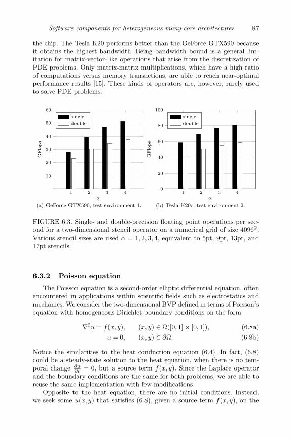
Software components for heterogeneous many-core architectures 87
the chip. The Tesla K20 performs better than the GeForce GTX590 becauseit obtains the highest bandwidth. Being bandwidth bound is a general lim-itation for matrix-vector-like operations that arise from the discretization ofPDE problems. Only matrix-matrix multiplications, which have a high ratioof computations versus memory transactions, are able to reach near-optimalperformance results [15]. These kinds of operators are, however, rarely usedto solve PDE problems.
1 2 3 4
10
20
30
40
50
60
α
GF
lops
single
double
(a) GeForce GTX590, test environment 1.
1 2 3 40
20
40
60
80
100
α
GF
lops
single
double
(b) Tesla K20c, test environment 2.
FIGURE 6.3. Single- and double-precision floating point operations per sec-ond for a two-dimensional stencil operator on a numerical grid of size 40962.Various stencil sizes are used α = 1, 2, 3, 4, equivalent to 5pt, 9pt, 13pt, and17pt stencils.
6.3.2 Poisson equation
The Poisson equation is a second-order elliptic differential equation, oftenencountered in applications within scientific fields such as electrostatics andmechanics. We consider the two-dimensional BVP defined in terms of Poisson’sequation with homogeneous Dirichlet boundary conditions on the form
∇2u = f(x, y), (x, y) ∈ Ω([0, 1]× [0, 1]), (6.8a)
u = 0, (x, y) ∈ ∂Ω. (6.8b)
Notice the similarities to the heat conduction equation (6.4). In fact, (6.8)could be a steady-state solution to the heat equation, when there is no tem-poral change ∂u
∂t = 0, but a source term f(x, y). Since the Laplace operatorand the boundary conditions are the same for both problems, we are able toreuse the same implementation with few modifications.
Opposite to the heat equation, there are no initial conditions. Instead,we seek some u(x, y) that satisfies (6.8), given a source term f(x, y), on the

88 Designing Scientific Applications on GPUs
right-hand side. For simplicity, assume that we know the exact solution, utrue,corresponding to (6.5). Then we use the method of manufactured solutions toderive an expression for the corresponding right-hand side f(x, y):
f(x, y) = ∇2utrue = −2π2 sin(πx) sin(πy). (6.9)
The spatial derivative in (6.8) is again approximated with finite differences,similar to the example in (6.2), except boundary values are explicitly set tozero. The discrete form of the system can now be written as a sparse linearsystem of equations:
Au = f , u, f ∈ RN , A ∈ RN×N , (6.10)
where A is the sparse matrix formed by finite difference coefficients, N is thenumber of unknowns, and f is given by (6.9). Equation (6.10) can be solvedin numerous ways, but a few observations may help do it more efficiently.Direct solvers based on Gaussian elimination are accurate and use a finitenumber of operations for a constant problem size. However, the arithmeticcomplexity grows with the problem size by as much as O(N3) and does notexploit the sparsity of A. Direct solvers are therefore mostly feasible for densesystems of limited sizes. Sparse direct solvers exist, but they are often difficultto parallelize, or applicable for only certain types of matrices. Regardless ofthe discretization technique, the discretization of an elliptic PDE into a linearsystem as in (6.10) yields a very sparse matrix A when N is large. Iterativemethods for solving large sparse linear systems find broad use in scientific ap-plications, because they require only an implementation of the matrix-vectorproduct, and they often use a limited amount of additional memory. Compre-hensive introductions to iterative methods may be found in any of [4, 13,23].
One benefit of the high abstraction level and the template-based librarydesign is to allow developers to implement their own components, such as iter-ative methods for solving sparse linear systems. The library includes three pop-ular iterative methods: conjugate gradient, defect correction, and geometricmultigrid. The conjugate gradient method is applicable only to systems withsymmetric positive definite matrices. This is true for the two-dimensional Pois-son problem, when it is discretized with a five-point finite difference stencil,because then there will be no off-centered approximations near the boundary.For high-order approximations (α > 1), we use the defect correction methodwith multigrid preconditioning. See e.g., [26] for details on multigrid methods.
We will not present the implementation details for all three methods butbriefly demonstrate the simplicity of implementing the body of such an itera-tive solver, given a textbook recipe or mathematical formulation. The defectcorrection method iteratively improves the solution to Ax = b, given an ini-tial start guess x0, by continuously solving a preconditioned error equation.The defect correction iteration can be written as
xk+1 = xk +M−1(b−Axk), A,M∈ RN×N , x,b ∈ RN , (6.11)

Software components for heterogeneous many-core architectures 89
where k is the iteration number and M is the preconditioner which shouldbe an approximation to the original coefficient matrix A. To achieve fast nu-merical convergence, applying the preconditioner should be a computationallyinexpensive operation compared to solving the original system. How to im-plement (6.11) within the library context is illustrated in Listing 6.8. Thehost CPU traverses each line in Listing 6.8 and tests for convergence, whilethe computationally expensive matrix-vector operation and preconditioning,can be executed on the GPU, if GPU-based components are used. The de-fect correction method has two attractive properties. First, global reductionis required to monitor convergence only once per iteration during convergenceevaluation, which reduces communication requirements and provides a ba-sis for efficient and scalable parallelization. Second, it has a minimal constantmemory footprint, making it a suitable method for solving very large systems.
Listing 6.8. main loop for the iterative defect correction solver: the solveris instantiated with template argument types for the matrix and vector classes,allowing underlying implementations to be based on GPU kernels
while ( r . nrm2 ( ) > t o l )
// Calculate residualA. mult (x , r ) ;
5 r . axpby (1 , −1, b) ;
// Reset i n i t i a l guessd . f i l l ( 0 ) ;
10 // Solve M∗d=rM(d , r ) ;
// Defect correction updatex . axpy (1 , d) ;
15
In the following section we demonstrate how to assemble a solver for thediscrete Poisson problem, using one of the three iterative methods to efficientlysolve (6.10).
6.3.2.1 Assembling the Poisson solver
Assembling the Poisson solver follows almost the same procedure as theheat conduction solver, except the time integration part is exchanged with aniterative method to solve the system of linear equations (6.10). For the discretematrix-vector product we reuse the Laplace operator from the heat conductionproblem in Listing 6.4 with few modifications. The Laplace operator is nowa matrix component, so to be compatible with the component interface rulesin Figure 6.1, a mult function taking two vector arguments is implementedinstead of the parentheses operator. We leave out this code example as italmost identical to the one in Listing 6.4.
At the beginning of the solver implementation we list the type definitionsfor the Poisson solver that will be used throughout the implementation. Herewe use a geometric multigrid method as a preconditioner for the defect cor-

90 Designing Scientific Applications on GPUs
rection method. Therefore the multigrid solver is assembled first, so that itcan be used in the assembling of the defect correction solver. Listing 6.9 de-fines the types for the vector, the matrix, the multigrid preconditioner, andthe defect correction solver. The geometric multigrid method needs two addi-tional template arguments that are specific for multigrid, namely, a smootherand a grid restriction/interpolation operator. These arguments are free to beimplemented and supplied by the developer if special care is required, e.g.,for a custom grid structure. For the Poisson problem on a regular grid, thelibrary contains built-in restriction and interpolation operators, and a red-black Gauss-Seidel smoother. We refer the reader to [26] for extensive detailson multigrid methods. The monitor and config types that appear in Listing 6.9are used for convergence monitoring within the iterative solver and to controlruntime parameters, such as tolerances and iteration limits.
Listing 6.9. type definitions for the Laplacian matrix component and themultigrid preconditioned iterative defect correction solver
typedef double va lue type ;typedef gpulab : : gr id<value type> vec to r type ;typedef l ap l a c i an<vector type> matr ix type ;
5 // MULTIGRID solver typestypedef gpulab : : s o l v e r s : : mu l t i g r id type s<
vec to r type, matr ix type, gpulab : : s o l v e r s : : g a u s s s e i d e l r b 2 d
10 , gpulab : : s o l v e r s : : g r id hand l e r 2d> mg types ;typedef gpulab : : s o l v e r s : : mult igr id<mg types> mg so lver type ;typedef mg so lver type : : monitor type monitor type ;typedef monitor type : : c o n f i g t y p e c o n f i g t y p e ;
15 // DC solver typestypedef gpulab : : s o l v e r s : : d e f e c t c o r r e c t i o n t y p e s<
vec to r type, matr ix type, monitor type
20 , mg so lver type> dc types ;typedef gpulab : : s o l v e r s : : d e f e c t c o r r e c t i o n<dc types> d c s o l v e r t y p e ;
With the type definitions set up, the implementation for the Poisson solverfollows in Listing 6.10. Some of the initializations are left out, as they followthe same procedure as for the heat conduction example. The defect correctionand geometric multigrid solvers are initialized and then multigrid is set as apreconditioner to the defect correction method. Finally the system is solvedvia a call to solve().

Software components for heterogeneous many-core architectures 91
Listing 6.10. initializing the preconditioned defect correction solver to ap-proximate the solution to Au = f
matr ix type A( alpha ) ; // High−order matrixmatr ix type M(1) ; // Low−order matrix
/∗ Omitted : create and in i t vectors u, f ∗/5
c o n f i g t y p e c o n f i g ; // Create configurationc o n f i g . s e t ("iter" , 30) ; // Set max iteration countc o n f i g . s e t ("rtol" ,1 e−10) ; // Set relat ive tolerancemonitor type monitor ( c o n f i g ) ; // Create monitor
10 d c s o l v e r t y p e s o l v e r (A, monitor ) ; // Create DC solvermg so lver type precond (M, monitor ) ; // Create MG preconditioners o l v e r . s e t p r e c o n d i t i o n e r ( precond ) ; // Set preconditioners o l v e r . s o l v e (u , f ) ; // Solve M −1(Au = f )i f ( monitor . converged ( ) )
15 p r i n t f ("SUCCESS\n" ) ;
6.3.2.2 Numerical solutions to the Poisson problem
The discrete Poisson problem (6.10) has been solved using the three itera-tive methods presented above. Convergence histories for the conjugate gradi-ent method and geometric multigrid method, using two different resolutions,are illustrated in Figure 6.4(a). Multigrid methods are very robust and algo-rithmic efficient, independent of the problem size. Figure 6.4(a) confirms thatthe rate of convergence for the multigrid method is unchanged for both prob-lem sizes. Only the attainable accuracy is slightly worsened, as a consequenceof a more ill-conditioned system for large problem sizes.
Defect correction in combination with multigrid preconditioning enablesefficient solution of high-order approximations of the Poisson problem, illus-trated in Figure 6.4(b). The multigrid preconditioning matrixM is based on alow-order approximation to (6.10), whereas matrix A is a high-order approx-imation. When M is a close approximation to A, defect correction convergesmost rapidly. This is the effect that can be seen between the three convergencelines in Figure 6.4(b).
6.4 Optimization strategies for multi-GPU systems
CUDA-enabled GPUs are optimized for high memory bandwidth and faston-chip performance. However, the role as a separate coprocessor to the CPUcan be a limiting factor for large scale scientific applications, because theGPU memory capacity is fixed and is only in the range of a few gigabytes. Incomparison, it is not unusual for a high-end workstation to be equipped with∼ 32GB of main memory, plus a terabyte hard disk capacity for secondarystorage. Therefore, large scale scientific applications that process gigabytes ofdata, require distributed computations on multiple GPU devices. Multi-GPU

92 Designing Scientific Applications on GPUs
0 5 10 1510
−14
10−12
10−10
10−8
10−6
10−4
10−2
100
Iteration
||r||2
CG, 1292
CG, 5132
MG, 1292
MG, 5132
(a) Convergence histories for the conjugategradient (CG) and multigrid (MG) meth-ods, for two different problem sizes.
0 10 20 30 4010
−20
10−15
10−10
10−5
100
Iteration
||r||2
α = 1
α = 2
α = 3
(b) Defect correction convergence historyfor three different stencil sizes.
FIGURE 6.4. Algorithmic performance for the conjugate gradient, multigrid,and defect correction methods, measured in terms of the relative residual periteration.
desktop computers and clusters can have a very attractive peak performance,but the addition of multiple devices introduces the potential performancebottleneck of slow data transfers across PCIe busses and network intercon-nections, as illustrated in Figure 6.5. The ratio between data transfers andcomputational work has a significant impact on the possibility for latencyhiding and thereby overall application performance.
Device memory Device memory
Host memory Host memory
kernel kernel
PCIe
Network
PCIeGPUDirect
FIGURE 6.5. Message passing between two GPUs involves several memorytransfers across lower bandwidth connections. The kernel call is required if thedata is not already sequentially stored in device memory. Recent generations ofNVIDIA GPUs, CUDA, and MPI support direct transfers without explicitelytransfering data to the host first.
Developing applications that exploit the full computational capabilities ofmodern clusters–GPU-based or not–is no trivial matter. Developers are facedwith the complexity of distributing and coordinating computations on nodesconsisting of many-core CPUs, GPUs, and potentially other types of acceler-ators as well. These complexities give rise to challenges in finding numerical

Software components for heterogeneous many-core architectures 93
algorithms, that are well suited for such systems, forcing developers to searchfor novel methods that utilize concurrency.
To ease software development, we use MPI-2 for message passing and en-sure a safe and private communication space by creation of a communicatorprivate to the library during initialization, as recommended by Hoefler andSnir [12]. With the addition of remote direct memory access (RDMA) forGPUDirect it is possible to make direct memory transfers between recent gen-eration of GPUs (Kepler), eliminating CPU overhead. Unfortunately there aresome strict system and driver requirements to enable these features. Therefore,in the following examples, device memory is first transferred to the CPU mainmemory before invoking any MPI calls. The library provides device-to-devicetransfers via template-based routines that work directly with GPU vector ob-jects. This hides the complexity of message passing from the developer andhelps developers design new components for multi-GPU execution.
In the following sections we present two very different methods for dis-tributed computing based on spatial and temporal decomposition. Eachmethod has its own characteristic, which makes the method attractive forvarious types of PDE problems and for different problem sizes.
6.4.1 Spatial domain decomposition
Domain decomposition methods can be used for distributing computa-tional work in the numerical solution of boundary value problems [25]. Thesemethods add parallelism by splitting the spatial dimensions, on which theboundary values are defined, into a number of smaller boundary value prob-lems and then coordinating the solution between adjacent subdomains. Do-main decomposition techniques, such as the classical overlapping Schwarzmethods, may be considered as preconditioners to the system of equationsthat arise from the discretization of PDEs, e.g., as for the Poisson problemin (6.10). The algorithmic efficiency of such methods depends on the size ofthe domain overlaps, while an additional coarse grid correction method issometimes necessary to maintain fast global convergence.
An alternative to the preconditioning strategy is to have each subdomainquery information from adjacent subdomains whenever needed. For PDEs thatare discretized onto regular shaped grids, this can be an attractive strategy,as the decomposition of subdomains, and thereby the communication topol-ogy, is straightforward. The library supports decomposition of regular gridsby either pre- or user-defined topologies. A topology in this context, is a de-scription of connectivity between processors that share the same grid alongwith information about the local and global discretization. Layers of ghostpoints are inserted at the artificially introduced boundaries to account forgrid points that reside in adjacent subdomains. The ghost point values can beupdated upon request from the user. An illustrative example is given in Figure6.6; the arrows indicate message passing between adjacent subdomains, whenupdating grid points within the ghost layers.

94 Designing Scientific Applications on GPUs
FIGURE 6.6. Domain distribution of a two-dimensional grid into three sub-domains. • and represent internal grid points and ghost points, respectively.
Topologies are introduced via an extra template argument to the grid class.A grid is by default not decomposed, because the default template argumentis based on a nondistribution topology implementation. The grid class is ex-tended with a new member function update(), which makes sure that allghost points are updated according to the grid topology. The library containstopologies based on one-dimensional and two-dimensional distributions of thegrid. The number of grid subdomains will be equal to the number of MPIprocesses executing the program.
If grid ghost layers are updated whenever information from adjacent sub-domains is needed, e.g., before a stencil operation, all interior points will beexactly the same as they would be for the nondistributed setup. Therefore,one advantage of this approach is that the algorithmic efficiency of an appli-cation can be preserved, if grid updates are consistently invoked at the propertimes.
Distributed performance for the finite difference stencil operation is il-lustrated in Figure 6.7. The timings include the compute time for the finitedifference approximation and the time for updating ghost layers via messagepassing. It is obvious from Figure 6.7(a) that communication overhead domi-nates for the smallest problem sizes, where the nondistributed grid (1 GPU) isfastest. However, communication overhead does not grow as rapidly as com-putation times, due to the surface-to-volume ratio. Therefore message pass-ing becomes less influential for large problems, where reasonable performancespeedups are obtained. Figure 6.7(b) demonstrates how the computationalperformance on multi-GPU systems can be significantly improved for variousstencil sizes. With this simple domain decomposition technique, developersare able to implement applications based on heterogeneous distributed com-puting, without explicitly dealing with message passing and it is still possibleto provide user specific implementations of the topology class for customizedgrid updates.

Software components for heterogeneous many-core architectures 95
104 105 106 107 10810−5
10−4
10−3
10−2
10−1
N
Tim
e[s
]
1 GPU
2 GPUs
4 GPUs
8 GPUs
16 GPUs
32 GPUs
(a) Absolute timings, α = 3.
1 2 3 40
200
400
600
α
GF
lops
1 GPU
2 GPUs
4 GPUs
8 GPUs
16 GPUs
32 GPUs
(b) Performance at N = 40692, single-precision.
FIGURE 6.7. Performance timings for distributed stencil operations, includingcommunication and computation times. Executed on test environment 3.
6.4.2 Parareal–parallel time integration
The use of spatial domain decomposition methods is widespread, as theyhave proven to be efficient on a wide range of problems. Unfortunately, appli-cations that are concerned with limited numerical problem sizes can rapidlyreach a speedup limit for a low number of processors due to scalability degra-dation when the number of processors becomes large, as this leads to anincreasingly unfavourable communication-to-compute ratio. This issue is con-tinuously worsened by the fact that communication speed has been increasingat a far slower pace than compute speed for the past several years, and thistrend is expected to continue for years to come. It is often referred to asthe memory wall [1], one of the grand challenges facing development and ar-chitectural design of future high-performance systems [8, 14]. Also, there areapplications based on ordinary differential equations, where classical domaindecomposition methods are not even applicable [19]. For these type of appli-cations, a method of adding parallelism in the temporal integration is of greatinterest. Contrary to space however, time is–by its very nature–sequential,which precludes a straightforward implementation of a parallel approach.
One method that introduces concurrency to the solution of evolution prob-lems is the parareal algorithm. Parareal is an iterative method imposed on atime decomposition. Gander and Vandewalle showed in [11] that the algo-rithm can be written both as a multiple shooting method and as a two-levelmultigrid-in-time approach, even though the leading idea came from spatialdomain decomposition. The method has many exciting features: it is fault

96 Designing Scientific Applications on GPUs
tolerant and has different communication characteristics than those of theclassical domain decomposition methods. It has also been demonstrated towork effectively on a wide range of problems, and most importantly, once theproper distribution infrastructure is in place, it can easily be wrapped aroundany type of numerical integrator, for any type of initial value problem.
6.4.2.1 The parareal algorithm
The parareal algorithm was first presented in 2001, in a paper by Lionset al. [18], and later introduced in a slightly revised predictor-corrector formin 2002 by Baffico et al. [3]. The parareal-in-time approach proposes to breakthe global problem of time evolution into a series of independent evolutionproblems on smaller intervals, see Figure 6.8. Initial states for these problems
T0 T1 TN TN+1
Space
T ime
GPU 1 GPU N
FIGURE 6.8. Time domain decomposition. A compute node is assigned toeach individual time subdomain to compute the initial value problem. Consis-tency at the time subdomain boundaries is obtained with the application ofa computationally cheap integrator in conjunction with the parareal iterativepredictor-corrector algorithm.
are needed and supplied by a simple, less accurate, but computationally cheapsequential integrator. The smaller independent evolution problems can thenbe solved in parallel. The information, generated during the concurrent so-lution of the independent evolution problems with accurate propagators andinaccurate initial states, is used in a predictor-corrector fashion in conjunctionwith the coarse integrator to propagate the solution faster, now using the in-formation generated in parallel. We define the decomposition into N intervals,that is,
T0 < T1 < · · · < Tn = n∆T < Tn+1 < TN , (6.12)

Software components for heterogeneous many-core architectures 97
where ∆T is the size of the time intervals and n = 0, 1, . . . , N . The generalinitial value problem on the decomposed time domain is defined as
∂u
dt+Au = 0, u(T0) = u0, t ∈ [T0, TN ] , (6.13)
where A is an operator from one Hilbert space to another. To solve the differ-ential problem (6.13) we define an operator F∆T that operates on some initialstate Un ≈ u(Tn) and returns an approximate solution to (6.13), at timeTn + ∆T . Such an operator is achieved by the implementation of a numeri-cal time integrator, using some small time-step δt ∆T in the integration.The numerical solution to (6.13) can then be obtained by applying the finepropagator sequentially for n = 1, 2, . . . , N .
Un = F∆T
(Tn−1, Un−1
), U0 = u0. (6.14)
For the purpose of parallel acceleration of the otherwise purely sequentialprocess of obtaining FN∆Tu0 ≈ u(TN ), we define the coarse propagator G∆T .G∆T also operates on some initial state Un, propagating the solution over thetime interval ∆T , but now using a time step δT . Typically δt < δT < ∆T .For the parareal algorithm to be effective, the coarse propagator G∆T has tobe substantially faster to evaluate than the fine propagator F∆T . There aremany ways of constructing the coarse propagator, the simplest one being toapply the same numerical integrator as for the fine propagator, but using acoarser time discretization. We refer the reader to [20] for an introduction toother methods. The coarse operator reads
Un = G∆T
(Tn−1, Un−1
), U0 = u0. (6.15)
Using the defined F∆T and G∆T operators, the predictor-corrector form of theparareal algorithm can be written in a single line as
Uk+1n = G∆T
(Uk+1n−1
)+ F∆T
(Ukn−1
)− G∆T
(Ukn−1
), Uk0 = u0, (6.16)
with the initial prediction U0n = Gn∆Tu0 for n = 1 . . . N and k = 1 . . .K. N
being the number of time subdomains, while K ≥ 1 is the number of predictor-corrector iterations applied. The parareal algorithm is implemented in the li-brary as a separate time-integration component, using a fully distributed workscheduling model, as proposed by Aubanel [2]. The model is schematically pre-sented in Figure 6.9. The parareal component hides all communication andwork distribution from the application developer. It is defined such that a useronly has to decide what coarse and fine propagators to use. Setting up thetype definitions for parareal time-integration using forward Euler for coarsepropagation and fourth order Runge-Kutta for fine propagation could thenbe defined as in Listing 6.11. The number of GPUs used for parallelizationdepends on the number of MPI processes executing the application.

98 Designing Scientific Applications on GPUs
Listing 6.11. assembling a parareal time integrator using forward Euler forcoarse propagation and a Runge-Kutta method for fine propagation
typedef gpulab : : i n t e g r a t i o n : : f o rwa rd eu l e r coa r s e ;typedef gpulab : : i n t e g r a t i o n : : ERK4 f i n e ;typedef gpulab : : i n t e g r a t i o n : : pararea l<coarse , f i n e> i n t e g r a t o r ;
Time
Iter. k = 0 Iter. k = 1 Iter. k = 2 Iter. k = 3
GPU. 1
GPU. 2
GPU. 3
GPU. 4
GPU. 5
GPU. 6
TG
TG
TG
TG
TG
TG
TF
TF
TF
TF
TF
TF
TG
TG
TG
TG
TG
TF
TF
TF
TF
TF
TG
TG
TG
TG
TF
TF
TF
TF
TG
TG
TG
FIGURE 6.9. Schematic visualization of a fully distributed work schedulingmodel for the parareal algorithm as proposed by Aubanel [2]. Each GPUis responsible for computing the solution on a single time subdomain. Thecomputation is initiated at rank 0 and cascades through to rank N where thefinal solution can be fetched.
6.4.2.2 Computational complexity
In the analysis of the computational complexity, we first recognize thatboth the coarse and the fine propagators, regardless of the type of discretiza-tion scheme, involve a complexity that is proportional to the number of timesteps being used. Let us define two scalar values CF and CG as the computa-tional cost of performing a single step with the fine and coarse propagators.The computational complexity of a propagator integrating over an interval∆T is then given by CF ∆T
δt and CG ∆TδT , respectively. R is introduced as the
relation between the two; that is, R is a measure of how much faster the coarsepropagator is compared to the fine propagator in integrating the time inter-val ∆T . The total computational cost for parareal over N intervals is thenproportional to
(k + 1)NCG∆T
δT+ kNCF
∆T
δt. (6.17)
Recognizing that the second term can be distributed over N processors, weare left with
(k + 1)NCG∆T
δT+ kCF
∆T
δt. (6.18)

Software components for heterogeneous many-core architectures 99
The above should be compared to the computational complexity of a purelysequential propagation, using only the fine operator,
TN − T0
δtCF = N
∆T
δtCF . (6.19)
We can now estimate the speedup, here denoted ψ, as the ratio between thecomputational complexity of the purely sequential solution, and the complex-ity of the solution obtained by the parareal algorithm (6.18). Neglecting theinfluence of communication speed and correction time, we are left with theestimate
ψ =N ∆T
δt CF(k + 1)NCG ∆T
δT + kCF ∆Tδt
=N
(k + 1)N CGCFδtδT + k
. (6.20)
If we additionally assume that the time spent on coarse propagation is neg-ligible compared to the time spent on the fine propagation, i.e., the limitCGCF
δtδT → 0, the estimate reduces to ψ = N
k . It is thus clear that the numberof iterations k for the algorithm to converge poses an upper bound on ob-tainable parallel efficiency. The number of iterations needed for convergenceis intimately coupled with the ratio R between the speed of the fine and thecoarse integrators CFCG
δTδt . Using a slow, but more accurate coarse integrator
will lead to convergence in fewer iterations k, but at the same time it alsomakes R smaller. Ultimately, this will degrade the obtained speedup as canbe deduced from (6.20), and by Amdahl’s law it will also lower the upperbound on possible attainable speedup. Thus, R cannot be made arbitrarilylarge since the ratio is inversely proportional to the number of iterations kneeded for convergence. This poses a challenge in obtaining speedup and is atrade-off between time spent on the fundamentally sequential part of the algo-rithm and the number of iterations needed for convergence. It is particularlyimportant to consider this trade-off in the choice of stopping strategy; a morethorough discussion on this topic is available in [20] for the interested reader.Measurements on parallel efficiency are typically observed in the literature tobe in the range of 20–50%, depending on the problem and the number of timesubdomains, which is also confirmed by our measurements using GPUs. Herewe include a demonstration of the obtained speedup of parareal applied to thetwo-dimensional heat problem (6.4). In Figure 6.10 the iterations needed forconvergence using the forward Euler method for both fine and coarse integra-tion are presented. R is regulated by changing the time step size for the coarseintegrator. In Figure 6.11 speedup and parallel efficiency measurements arepresented. Notice, when using many GPUs it is advantageous to use a faster,less accurate coarse propagator, despite it requires an extra parareal iterationthat increases the total computational complexity.

100 Designing Scientific Applications on GPUs
0
100
0
10
20
0.5
1·10−2
RGPUs
||ere
l||∞
(a) The relative error after one parareal it-eration (k = 1).
50100
15010
201
2
3
RGPUs
k
(b) Iterations K needed to obtain a relativeerror less than 10−5.
FIGURE 6.10. Parareal convergence properties as a function of R and numberof GPUs used. The error is measured as the relative difference between thepurely sequential solution and the parareal solution.
0 50 100 1500
10
200
5
10
RGPUs
Sp
eedup
(a) Measured parallel speedup
0 50 100 1500
10
200
0.5
1
RGPUs
Effi
cien
cy
(b) Measured parallel efficiency
FIGURE 6.11. Parareal performance properties as a function of R and numberGPUs used. Notice how the obtained performance depends greatly on thechoice ofR as a function of the number of GPUs. Executed on test environment3.
6.5 Conclusion and outlook
Massively parallel heterogeneous systems continue to enter the consumermarket, and there has been no identification that this trend will stop for yearsto come. However, these parallel architectures require software vendors to ad-

Software components for heterogeneous many-core architectures 101
just to new programming models and optimization strategies. Good softwarelibraries are important tools for reducing the time and complexity of adjustingto new architectures, and they provide the user with an intuitive programminginterface.
We have presented ideas for a generic GPU-based library for fast assem-bling of PDE solvers. A high-level interface and simple implementation con-cepts were created with the objective of enhancing developer productivity andto ensure performance portability. Two elementary PDE model problems wereused to demonstrate assembling of both spatial and temporal approximationtechniques. Results confirmed that numerical methods for solution of PDEsystems are bandwidth limited on GPU systems. Therefore higher-order meth-ods can be advantageous, when extra computational work can be performedduring memory transfer idle times, leading to increased flop performance.
Decomposition strategies for spatial and temporal parallelization on multi-GPU systems have been presented, with reasonable performance speedups.Novel results for the parareal algorithm on multi-GPU systems have been pre-sented, and an example of parallel efficiency for the heat conduction problemhas been demonstrated. Furthermore, a domain decomposition technique thatpreserves algorithmic efficiency has been presented for the Poisson problem.
The library has already successfully been used for development of a fasttool intended for scientific applications within maritime engineering; see Chap-ter 11 for details. We intend to further extend the library, as we explore newtechniques, suitable for parallelization on heterogeneous systems, that fit thescope of our applications.
For more information about the library and our work within the GPUlabgroup at the Technical University of Denmark, we encourage you to visithttp://gpulab.imm.dtu.dk
Acknowledgments
This work have been supported by grant no. 09-070032 from the DanishResearch Council for Technology and Production Sciences. A special thanksgoes to Professor Jan S. Hesthaven for supporting parts of this work. Scala-bility and performance tests were done in the GPUlab at DTU Informatics,Technical University of Denmark and using the GPU-cluster at the Centerfor Computing and Visualization, Brown University, USA. The NVIDIA Cor-poration is acknowledged for generous hardware donations to facilities of theGPUlab.

102 Designing Scientific Applications on GPUs
Bibliography
[1] K. Asanovic, R. Bodik, B. C. Catanzaro, J. J. Gebis, P. Husbands,K. Keutzer, D. A. Patterson, W. L. Plishker, J. Shalf, S. W. Williams, andK. A. Yelick. The landscape of parallel computing research: A view fromBerkeley. Technical Report UCB/EECS-2006-183, EECS Department,University of California, Berkeley, Dec 2006.
[2] E. Aubanel. Scheduling of tasks in the parareal algorithm. ParallelComputing, 37:172–182, 2010.
[3] L. Baffico, S. Bernard, Y. Maday, G. Turinici, and G. Zerah. Parallel-in-time molecular-dynamics simulations. Phys. Rev. E, 66:057701, Nov2002.
[4] R. Barrett, M. Berry, T. F. Chan, J. Demmel, J. Donato, J. Dongarra,V. Eijkhout, R. Pozo, C. Romine, and H. Van der Vorst. Templates forthe Solution of Linear Systems: Building Blocks for Iterative Methods.SIAM, Philadelphia, PA, 2nd edition, 1994.
[5] N. Bell and M. Garland. Implementing sparse matrix-vector multipli-cation on throughput-oriented processors. In SC ’09: Proceedings of theConference on High Performance Computing Networking, Storage andAnalysis, pages 1–11, New York, NY, 2009. ACM.
[6] N. Bell and J. Hoberock. Thrust: A productivity-oriented library forCUDA. In GPU Computing Gems, Jade Edition, Edited by Wen-mei W.Hwu. Elsevier Science, 2:359–371, 2011.
[7] A. J. Chorin and J. E. Marsden. A Mathematical Introduction to FluidMechanics. Texts in Applied Mathematics. Springer, New York, NY, 3rdedition, 1993.
[8] P. Messina et. al D. L. Brown. Scientific grand challenges, crosscuttingtechnologies for computing at the exascale. Technical Report, U.S. De-partment of Energy, Washington, D.C., February 2010.
[9] J.H. Ferziger and M. Peric. Computational Methods for Fluid Dynamics.Numerical Methods: Research and Development. Springer-Verlag, BerlinHeidelberg New York, 1996.
[10] E. Gamma, R. Helm, R. Johnson, and J. Vlissides. Design Patterns–Elements of Reusable Object-Oriented Software. Addison-Wesley Profes-sional Computing Series, 1995.
[11] M. Gander and S. Vandewalle. Analysis of the parareal time-parallel time-integration method. SIAM Journal of Scientific Computing, 29(2):556–578, 2007.

Software components for heterogeneous many-core architectures 103
[12] T. Hoefler and M. Snir. Writing parallel libraries with MPI–Commonpractice, issues, and extensions. In Y. Cotronis, A. Danalis, D. Nikolopou-los, and J. Dongarra, editors, Recent Advances in the Message PassingInterface, volume 6960 of Lecture Notes in Computer Science, pages 345–355. Springer, Berlin/Heidelberg, 2011.
[13] C. T. Kelley. Iterative Methods for Linear and Nonlinear Equations. Fron-tiers in Applied Mathematics Series. Society for Industrial and AppliedMathematics, Philadelphia, PA,, 1995.
[14] D. E. Keyes. Exaflop/s: The why and the how. Comptes RendusMecanique, 339:70–77, 2011.
[15] D. B. Kirk and W.-M. W. Hwu. Programming Massively Parallel Pro-cessors: A Hands-on Approach. Morgan Kaufmann Publishers Inc., SanFrancisco, CA, 2010.
[16] T. Korson and J. D. McGregor. Technical criteria for the specificationand evaluation of object-oriented libraries. Softw. Eng. J., 7(2):85–94,March 1992.
[17] R. J. LeVeque. Finite Difference Methods for Ordinary and Partial Dif-ferential Equations–Steady-state and Time-dependent Problems. SIAM,Philadelphia, PA, 2007.
[18] J.-L. Lions, Y. Maday, and G. Turinici. Resolution d’edp par un schemaen temps parareel. C.R. Acad. Sci. Paris Ser. I Math, 332:661–668, 2001.
[19] Y. Maday. The parareal in time algorithm. Technical Report R08030,Universite Pierre et Marie Curie, Paris, 2008.
[20] A. S. Nielsen. Feasibility study of the parareal algorithm. Master thesis,Technical University of Denmark, Department of Informatics and Math-ematical Modeling, Lyngby, 2012.
[21] NVIDIA Corporation. CUDA C Programming Guide, 2012.
[22] NVIDIA Corporation. CUDA C Best Practices Guide, 2012.
[23] Y. Saad. Iterative Methods for Sparse Linear Systems. Society for Indus-trial and Applied Mathematics, Philadelphia, PA, 2nd edition, 2003.
[24] A. Skjellum, N. E. Doss, and P. V. Bangaloret. Writing libraries in MPI.Technical Report, Department of Computer Science and NSF EngineeringResearch Center for Computational Fiels Simulation. Mississippi StateUniversity, 1994.
[25] B. F. Smith, P. E. Bjørstad, and W. D. Gropp. Domain Decomposition:Parallel Multilevel Methods for Elliptic Partial Differential Equations.Cambridge University Press, New York, 1996.

104 Designing Scientific Applications on GPUs
[26] U. Trottenberg, C. W. Oosterlee, and A. Schuller. Multigrid. ElsevierAcademic Press, London, 2001.
[27] D. Vandevoorde and N. M. Josuttis. C++ Templates: The CompleteGuide. Addison-Wesley Professional, November 2002.

Chapter 7
Development methodologies for GPUand cluster of GPUs
Sylvain Contassot-Vivier
Universite Lorraine, Loria UMR 7503 & AlGorille INRIA Project Team,Nancy, France
Stephane Vialle
SUPELEC, UMI GT-CNRS 2958 & AlGorille INRIA Project Team, Metz,France
Jens Gustedt
INRIA Nancy–Grand Est, AlGorille INRIA Project Team, Strasbourg, France
7.1 Introduction . . . . . . . . . . . . . . . . . . . . . . . . . . . . . . . . . . . . . . . . . . . . . . . . . . . . . . 1067.2 General scheme of synchronous code with
computation/communication overlapping in GPU clusters . . . . . 1067.2.1 Synchronous parallel algorithms on GPU clusters . . . . . . 1067.2.2 Native overlap of CPU communications and GPU
computations . . . . . . . . . . . . . . . . . . . . . . . . . . . . . . . . . . . . . . . . . . . . 1087.2.3 Overlapping with sequences of transfers and
computations . . . . . . . . . . . . . . . . . . . . . . . . . . . . . . . . . . . . . . . . . . . . 1107.2.4 Interleaved communications-transfers-computations
overlapping . . . . . . . . . . . . . . . . . . . . . . . . . . . . . . . . . . . . . . . . . . . . . . 1157.2.5 Experimental validation . . . . . . . . . . . . . . . . . . . . . . . . . . . . . . . . . 118
7.3 General scheme of asynchronous parallel code withcomputation/communication overlapping . . . . . . . . . . . . . . . . . . . . . . . 1207.3.1 A basic asynchronous scheme . . . . . . . . . . . . . . . . . . . . . . . . . . . 1227.3.2 Synchronization of the asynchronous scheme . . . . . . . . . . . 1267.3.3 Asynchronous scheme using MPI, OpenMP, and CUDA 1307.3.4 Experimental validation . . . . . . . . . . . . . . . . . . . . . . . . . . . . . . . . . 137
7.4 Perspective: a unifying programming model . . . . . . . . . . . . . . . . . . . . . 1407.4.1 Resources . . . . . . . . . . . . . . . . . . . . . . . . . . . . . . . . . . . . . . . . . . . . . . . . 1417.4.2 Control . . . . . . . . . . . . . . . . . . . . . . . . . . . . . . . . . . . . . . . . . . . . . . . . . . . 1427.4.3 Example: block-cyclic matrix multiplication (MM) . . . . . 1427.4.4 Tasks and operations . . . . . . . . . . . . . . . . . . . . . . . . . . . . . . . . . . . . 145
7.5 Conclusion . . . . . . . . . . . . . . . . . . . . . . . . . . . . . . . . . . . . . . . . . . . . . . . . . . . . . . . . 1467.6 Glossary . . . . . . . . . . . . . . . . . . . . . . . . . . . . . . . . . . . . . . . . . . . . . . . . . . . . . . . . . . 146
105

106 Designing Scientific Applications on GPUs
Bibliography . . . . . . . . . . . . . . . . . . . . . . . . . . . . . . . . . . . . . . . . . . . . . . . . . . . . . . 147
7.1 Introduction
This chapter proposes to draw upon several development methodologies toobtain efficient codes in classical scientific applications. Those methodologiesare based on the feedback from several research works involving GPUs, eitherin a single machine or in a cluster of machines. Indeed, our past collaborationswith industries have allowed us to point out that in their economical context,they can adopt a parallel technology only if its implementation and main-tenance costs are small compared with the potential benefits (performance,accuracy, etc.). So, in such contexts, GPU programming is still regarded withsome distance due to its specific field of applicability (SIMD/SIMT model:Single Instruction Multiple Data/Thread) and its still higher programmingcomplexity and maintenance. In the academic domain, things are a bit differ-ent, but studies for efficiently integrating GPU computations in multicore clus-ters with maximal overlapping of computations with communications and/orother computations are still rare.
For these reasons, the major aim of that chapter is to propose generalprogramming patterns, as simple as possible, that can be followed or adaptedin practical implementations of parallel scientific applications. In addition, wepropose a prospect analysis together with a particular programming tool thatis intended to ease multicore GPU cluster programming.
7.2 General scheme of synchronous code with computa-tion/communication overlapping in GPU clusters
7.2.1 Synchronous parallel algorithms on GPU clusters
Considered parallel algorithms and implementations
This section focuses on synchronous parallel algorithms implemented withoverlapping computations and communications. Parallel synchronous algo-rithms are easier to implement, debug, and maintain than asynchronous ones(see Section 7.3). Usually, they follow a BSP-like parallel scheme (Bulk Syn-chronous Parallel model), alternating local computation steps and commu-nication steps (see [19]). Their execution is usually deterministic, except forstochastic algorithms that contain random number generations. Even in thiscase, their execution can be controlled during debug steps, allowing the userto track and to fix bugs quickly.

Development methodologies for GPU and cluster of GPUs 107
However, depending on the properties of the algorithm, it is sometimespossible to overlap computations and communications. If processes exchangedata that is not needed for the computation immediately following, it is pos-sible to implement such an overlap. We have investigated the efficiency of thisapproach in previous works [14,20], using standard parallel programming toolsto achieve the implementation.
The normalized and well-known Message Passing Interface (MPI) includessome asynchronous point-to-point communication routines, that should allowthe implementation of some communication/computation overlap. However,current MPI implementations do not achieve this goal efficiently; effectiveoverlapping with MPI requires a group of dedicated threads (in our case im-plemented with OpenMP) for the basic synchronous communications whileanother group of threads executes computations in parallel. Nevertheless,communication and computation are not completely independent on mod-ern multicore architectures: they use shared hardware components such asthe interconnection bus and the RAM. Therefore, this approach saves onlyup to 20% of the expected time on such a platform. This picture changes onclusters equipped with GPUs. Indeed, GPUs effectively allow independenceof computations they perform and communications done on the mainboard(CPU, interconnection bus, RAM, network card). We save up to 100% of theexpected time on our GPU cluster, as we will expose in the next section.
Specific interests in GPU clusters
In a computing node, a GPU is a kind of scientific coprocessor, usuallylocated on an auxiliary board, with its own memory. So, once data are trans-ferred from the CPU memory to the GPU memory, GPU computations canbe achieved on the GPU board, totally in parallel with any CPU activities(such as internode cluster communications). The CPU and the GPU accesstheir respective memories and do not interfere with each other, so they canachieve a very good overlap of their activities (better than two CPU cores).
But using a GPU on a computing node requires the transfer of data fromthe CPU to the GPU memory, as well as the transfer of the computationresults back from the GPU to the CPU. Transfer times are not excessive, butdepending on the application they still can be significant compared to theGPU computation times. So, sometimes it can be interesting to overlap theinternode cluster communications with both the CPU/GPU data transfersand the GPU computations. We can identify four main parallel programmingschemes on a GPU cluster:
1. parallelizing only internode CPU communications with GPU compu-tations, and achieving CPU/GPU data transfers before and after thisparallel step,
2. parallelizing internode CPU communications with a (sequential) se-quence of CPU/GPU data transfers and GPU computations,

108 Designing Scientific Applications on GPUs
.......
waiting
MPIpcomms GPU
threadexec.
CPU GPUMonothread CPU program
Sync.pCPUpppppppGPUpdataptransferppppppppppppppppppppppppppppp(defaultpstream)pp
Async.pGPUpparallelpcomputationpp
Sync.pinternodepCPUpcomms
pp
Sync.pGPUpppppppCPUpdataptransfer
FIGURE 7.1. Native overlap of internode CPU communications with GPUcomputations.
3. parallelizing internode CPU communications with a streamed sequenceof CPU/GPU data transfers and GPU computations,
4. parallelizing internode CPU communications with CPU/GPU datatransfers and with GPU computations, interleaving computation-communication iterations.
7.2.2 Native overlap of CPU communications and GPU com-putations
Using CUDA, GPU kernel executions are nonblocking, and GPU/CPUdata transfers are blocking or nonblocking operations. All GPU kernel exe-cutions and CPU/GPU data transfers are associated to “streams”, and alloperations on a same stream are serialized. When transferring data from theCPU to the GPU, then running GPU computations, and finally transferringresults from the GPU to the CPU, there is a natural synchronization andserialization if these operations are achieved on the same stream. GPU devel-opers can choose to use one (default) or several streams. In this first schemeof overlapping, we consider parallel codes using only one GPU stream.
“Nonblocking GPU kernel execution” means a CPU routine runs a parallelexecution of a GPU computing kernel, and the CPU routine continues itsexecution (on the CPU) while the GPU kernel is running (on the GPU).Then the CPU routine can initiate some communications with some otherCPUs, and so it automatically overlaps the internode CPU communicationswith the GPU computations (see Figure 7.1). This overlapping is natural whenprogramming with CUDA and MPI: it is easy to deploy, but does not overlapthe CPU/GPU data transfers.
Listing 7.1 introduces the generic code of a MPI+CUDA implementation,natively and implicitly overlapping MPI communications with CUDA GPUcomputations.

Development methodologies for GPU and cluster of GPUs 109
Listing 7.1. generic scheme implicitly overlapping MPI communications withCUDA GPU computations
// Input data and result variables and arrays (example with// f loat datatype , 1D input arrays , and scalar results )f loat ∗cpuInputTabAdr , ∗gpuInputTabAdr ;f loat ∗cpuResTabAdr , ∗gpuResAdr ;
5
// CPU and GPU array al locationscpuInputTabAdr = malloc ( s izeof ( f loat ) ∗N) ;cudaMalloc(&gpuInputTabAdr , s izeof ( f loat ) ∗N) ;cpuResTabAdr = malloc ( s izeof ( f loat ) ∗NbIter ) ;
10 cudaMalloc(&gpuResAdr , s izeof ( f loat ) ) ;
// Definition of the grid of blocks of GPU threadsdim3 Dg , Db;Dg . x = . . .
15 . . .
// Indexes of source and destination MPI processesint dest = . . .int s r c = . . .
20
// Computation loop (using the GPU)for ( int i = 0 ; i < NbIter ; i++)
cudaMemcpy( gpuInputTabAdr , cpuInputTabAdr , // Data transfer :s izeof ( f loat ) ∗N, // CPU −−> GPU (sync . op)
25 cudaMemcpyHostToDevice ) ;gpuKernel k1<<<Dg,Db>>>() ; // GPU comp. (async . op)MPI Sendrecv replace ( cpuInputTabAdr , // MPI comms. (sync . op)
N,MPI FLOAT,dest , 0 , src , 0 , . . . ) ;
30 // IF there i s (now) a result to transfer from the GPU to the CPU:cudaMemcpy( cpuResTabAdr + i , gpuResAdr , // Data transfer :
s izeof ( f loat ) , // GPU−−> CPU (sync . op)cudaMemcpyDeviceToHost ) ;
35 . . .
Some input data and output results arrays and variables are declared andallocated from line 3 through 10, and a computation loop is implemented fromline 22 through 34. At each iteration:
• cudaMemcpy on line 23 transfers data from the CPU memory to theGPU memory. This is a basic and synchronous data transfer.
• gpuKernel k1<<<Dg,Db>>> on line 26 starts GPU computation (run-ning a GPU kernel on the grid of blocks of threads defined in lines 13 to15). This is a standard GPU kernel run; it is an asynchronous operation.The CPU can continue to run its code.
• MPI Sendrecv replace on line 27 achieves some blocking internodecommunications, overlapping GPU computations started just previously.
• If needed, cudaMemcpy on line 31 transfers the iteration result fromone variable in the GPU memory to one array index in the CPU mem-ory (in this example the CPU collects all iteration results in an array).This operation is started after the end of the MPI communication (pre-vious instruction) and after the end of the GPU kernel execution. CUDA

110 Designing Scientific Applications on GPUs
2I-ISync.ICPUIIIIIIIGPUIIIIIIdataItransferI2I-IAsync.IGPUIparallelIIIIIIIcomputation
1I-ISynchronousIIIIIIIIIIIinternodeIIIIIIICPUIcomms
2I-ISync.IGPUIIIIIIICPUIIIIIIdataItransfer
.......
waiting
MPIIcomms
GPUthreadexec.
CPU GPUMultithreaded CPU program
CPU main thread next instructions
1 - threadcomm
2 - thread comput
CPU thread creation
CPU threadsynchonization barrier
II
FIGURE 7.2. Overlap of internode CPU communications with a sequence ofCPU/GPU data transfers and GPU computations.
insures an implicit synchronization of all operations involving the sameGPU stream, like the default stream in this example. The transfer of theresults has to wait until the GPU kernel execution is finished. If thereis no results transfer implemented, the next operation on the GPU willwait until the GPU kernel execution has ended.
This implementation is the easiest one involving the GPU. It achieves animplicit overlap of internode communications and GPU computations withno explicit multithreading required on the CPU. However, CPU/GPU datatransfers are achieved serially and not overlapped.
7.2.3 Overlapping with sequences of transfers and computa-tions
Overlapping with a sequential GPU sequence
When CPU/GPU data transfers are not negligible compared to GPU com-putations, it can be interesting to overlap internode CPU computations witha GPU sequence including CPU/GPU data transfers and GPU computations(see Figure 7.2). Algorithmic issues of this approach are basic, but their im-plementation requires explicit CPU multithreading and synchronization, andCPU data buffer duplication. We need to implement two threads, one start-ing and achieving MPI communications and the other running the GPU se-quence. OpenMP allows an easy and portable implementation of this overlap-ping strategy. However, it remains more complex to develop and to maintainthan the previous strategy (overlapping only internode CPU communicationsand GPU computations) and should be adopted only when CPU/GPU datatransfer times are not negligible.
Listing 7.2 introduces the generic code of a MPI+OpenMP+CUDA imple-mentation, explicitly overlapping MPI communications with GPU sequences.

Development methodologies for GPU and cluster of GPUs 111
Listing 7.2. generic scheme explicitly overlapping MPI communications withsequences of CUDA CPU/GPU transfers and CUDA GPU computations
// Input data and result variables and arrays (example with// f loat datatype , 1D input arrays , and scalar results )f loat ∗cpuInputTabAdrCurrent , ∗cpuInputTabAdrFuture , ∗gpuInputTabAdr ;f loat ∗cpuResTabAdr , ∗gpuResAdr ;
5
// CPU and GPU array al locationscpuInputTabAdrCurrent = malloc ( s izeof ( f loat ) ∗N) ;cpuInputTabAdrFuture = malloc ( s izeof ( f loat ) ∗N) ;cudaMalloc(&gpuInputTabAdr , s izeof ( f loat ) ∗N) ;
10 cpuResTabAdr = malloc ( s izeof ( f loat ) ∗NbIter ) ;cudaMalloc(&gpuResAdr , s izeof ( f loat ) ) ;
// Definition of the grid of blocks of GPU threadsdim3 Dg , Db;
15 Dg . x = . . .. . .
// Indexes of source and destination MPI processesint dest = . . .
20 int s r c = . . .
// Set the number of OpenMP threads ( to create ) to 2omp set num threads (2 ) ;// Create threads and start the paral le l OpenMP region
25 #pragma omp p a r a l l e l
// Buffer pointers (thread local variables )f loat ∗ cur rent = cpuInputTabAdrCurrent ;f loat ∗ f u tu r e = cpuInputTabAdrFuture ;
30 f loat ∗tmp ;
// Computation loop (using the GPU)for ( int i = 0 ; i < NbIter ; i++)
35 // − Thread 0: achieves MPI communicationsi f ( omp get thread num () == 0)
MPI Sendrecv ( current , // MPI comms. (sync . op)N, MPI FLOAT, dest , 0 ,future ,
40 N, MPI FLOAT, dest , 0 , . . . ) ;
// − Thread 1: achieves the GPU sequence (GPU computations and// CPU/GPU data transfers ) else i f ( omp get thread num () == 1)
45 cudaMemcpy( gpuInputTabAdr , current , // Data transfer :s izeof ( f loat ) ∗N, // CPU −−> GPU (sync . op)cudaMemcpyHostToDevice ) ;
gpuKernel k1<<<Dg,Db>>>() ; // GPU comp. (async . op)// IF there i s (now) a result to transfer from the GPU to the CPU:
50 cudaMemcpy( cpuResTabAdr + i , gpuResAdr , // Data transfer :s izeof ( f loat ) , // GPU−−> CPU (sync . op)cudaMemcpyDeviceToHost ) ;
55 // − Wait until both threads have achieved their iteration tasks#pragma omp b a r r i e r// − Each thread permutes i t s local buffer pointerstmp = current ;cur rent = fu tu r e ;
60 f u tu r e = tmp ; // End of computation loop
// End of OpenMP paral le l region. . .

112 Designing Scientific Applications on GPUs
Lines 25–62 implement the OpenMP parallel region, around the compu-tation loop (lines 33–61). For efficient performances it is important to createand destroy threads only one time (not at each iteration): the parallel regionhas to surround the computation loop. Lines 3–11 consist of declaration andallocation of input data arrays and result arrays and variables, as in the pre-vious algorithm (Listing 7.1). However, we implement two input data bufferson the CPU (current and future version). As we aim to overlap internode MPIcommunications and GPU sequence, including CPU to GPU data transfer ofcurrent input data array, we need to store the received new input data arrayin a separate buffer. Then, the current input data array will be safely read onthe CPU and copied into the GPU memory.
The thread creations are easily achieved with one OpenMP directive(line 25). Then each thread defines and initializes its local buffer pointers,and enters its computing loop (lines 28–33). Inside the computing loop, a teston the thread number makes it possible to run a different code in each thread.Lines 37–40 implement the MPI synchronous communication run by threadnumber 0. Lines 45–52 implement the GPU sequence run by thread 1: CPUto GPU data transfer, GPU computation, and GPU to CPU result transfer(if needed). Details of the three operations of this sequence have not changedfrom the previous overlapping strategy.
At the end of Listing 7.2, an OpenMP synchronization barrier on line 56forces the OpenMP threads to wait until MPI communications and GPUsequence are achieved. Then, each thread permutes its local buffer pointers(lines 58–60), and is ready to enter the next iteration, processing the newcurrent input array.
Overlapping with a streamed GPU sequence
Depending on the algorithm implemented, it is sometimes possible to splitthe GPU computation into several parts processing distinct data. Then, we canspeedup the GPU sequence using several CUDA streams. The goal is to overlapCPU/GPU data transfers with GPU computations inside the GPU sequence.Compared to the previous overlapping strategy, we have to split the initial datatransfer into a set of n asynchronous and smaller data transfers, and split theinitial GPU kernel call into a set of n calls to the same GPU kernel. Usually,these smaller calls are deployed with fewer GPU threads (i.e., associated toa smaller grid of blocks of threads). Then, the first GPU computations canstart as soon as the first data transfer has been achieved, and next transferscan be done in parallel with next GPU computations (see Figure 7.3).
NVIDIA advises starting all asynchronous CUDA data transfers and thencalling all CUDA kernel executions, using up to 16 streams [16]. Then, theCUDA driver and runtime optimize the global execution of these operations.So, we accumulate two overlapping mechanisms. The former is controlled byCPU multithreading and overlaps MPI communications and the streamedGPU sequence. The latter is controlled by CUDA programming and overlapsCPU/GPU data transfers and GPU computations. Again, OpenMP allows

Development methodologies for GPU and cluster of GPUs 113
2I-IAsync.ICPUIIIIIIIGPUIIIIIIdataItransfersIonIstreamsI2I-IAsync.IGPUIparallelIIIIIIIcomputationsIonIstreams
1I-ISynchronousIIIIIIIIIIIinternodeIIIIIIICPUIcomms
2I-IAsync.IGPUIIIIIIICPUIIIIIIdataItransfersIonIstreams
waiting
MPIIcomms
GPUthreadexec.
CPU GPUMultithreaded CPU program
CPU main thread next instructions
1 - threadcomm
2 - thread comput
CPU thread creation
CPU threadsynchonization barrier
II
AutomaticIresynchronizationonIeachIstream
FIGURE 7.3. Overlap of internode CPU communications with a streamedsequence of CPU/GPU data transfers and GPU computations.
the easy implementation of the CPU multithreading and waiting for the endof both CPU threads before executing the next instructions of the code.
Listing 7.3 introduces the generic MPI+OpenMP+CUDA code, explicitlyoverlapping MPI communications with streamed GPU sequences.
Listing 7.3. generic scheme explicitly overlapping MPI communications withstreamed sequences of CUDA CPU/GPU transfers and CUDA GPU computa-tions
// Input data and result variables and arrays (example with// f loat datatype , 1D input arrays , and scalar results )f loat ∗cpuInputTabAdrCurrent , ∗cpuInputTabAdrFuture , ∗gpuInputTabAdr ;f loat ∗cpuResTabAdr , ∗gpuResAdr ;
5 // CPU and GPU array al locations ( al locates page−locked CPU memory)cudaHostAlloc(&cpuInputTabAdrCurrent , s izeof ( f loat ) ∗N,
cudaHostAl locDefault ) ;cudaHostAlloc(&cpuInputTabAdrFuture , s izeof ( f loat ) ∗N,
cudaHostAl locDefault ) ;cudaMalloc(&gpuInputTabAdr , s izeof ( f loat ) ∗N) ;cpuResTabAdr = malloc ( s izeof ( f loat ) ∗NbIter ) ;
10 cudaMalloc(&gpuResAdr , s izeof ( f loat ) ) ;// Stream declaration and creationcudaStream t TabS [ NbS ] ;for ( int s = 0 ; s < NbS ; s++)
cudaStreamCreate(&TabS [ s ] ) ;15 // Definition of the grid of blocks of GPU threads
. . .// Set the number of OpenMP threads ( to create ) to 2omp set num threads (2 ) ;// Create threads and start the paral le l OpenMP region
20 #pragma omp p a r a l l e l
// Buffer pointers (thread local variables )f loat ∗ cur rent = cpuInputTabAdrCurrent ;f loat ∗ f u tu r e = cpuInputTabAdrFuture ;
25 f loat ∗tmp ;// Stride of data processed per streamint s t r i d e = N/NbS ;// Computation loop (using the GPU)for ( int i = 0 ; i < NbIter ; i++)
30 // − Thread 0: achieves MPI communicationsi f ( omp get thread num () == 0)

114 Designing Scientific Applications on GPUs
MPI Sendrecv ( current , // MPI comms. (sync . op)N, MPI FLOAT, dest , 0 ,future ,
35 N, MPI FLOAT, dest , 0 , . . . ) ;// − Thread 1: achieves the streamed GPU sequence (GPU// computations and CPU/GPU data transfers ) else i f ( omp get thread num () == 1)
for ( int s = 0 ; s < NbS ; s++) // Start a l l data transfers :40 cudaMemcpyAsync ( gpuInputTabAdr + s ∗ s t r i d e , // CPU −−> GPU
cur rent + s ∗ s t r i d e , // (async . ops)s izeof ( f loat ) ∗ s t r i d e ,cudaMemcpyHostToDevice ,TabS [ s ] ) ;
45 for ( int s = 0 ; s < NbS ; s++) // Start a l l GPU comps. (async . )
gpuKernel k1<<<Dg, Db, 0 , TabS [ s]>>>(gpuInputTabAdr + s ∗ s t r i d e) ;
cudaThreadSynchronize ( ) ; // Wait a l l threads are ended
50 // IF there i s (now) a result to transfer from the GPU to the CPU:cudaMemcpy( cpuResTabAdr , // Data transfers :
gpuResAdr , // GPU−−> CPU (sync . op)s izeof ( f loat ) ,cudaMemcpyDeviceToHost ) ;
55 // − Wait until both threads have achieved their iteration tasks#pragma omp b a r r i e r// − Each thread permutes i t s local buffer pointerstmp = current ; cur rent = fu tu r e ; f u tu r e = tmp ;
60 // End of computation loop // End of OpenMP paral le l region. . .// Destroy the streamsfor ( int s = 0 ; s < NbS ; s++)
65 cudaStreamDestroy (TabS [ s ] ) ;. . .
Efficient usage of CUDA streams requires executing asynchronousCPU/GPU data transfers, which implies reading page-locked data in CPUmemory. So, CPU memory allocations on lines 6 and 7 are implemented withcudaHostAlloc instead of the basic malloc function. Then, NbS streamsare created on lines 12–14. Usually we create 16 streams: the maximum num-ber supported by CUDA.
An OpenMP parallel region including two threads is implemented onlines 18–61 of Listing 7.3, as in the previous algorithm (see Listing 7.2). Codeof thread 0 achieving MPI communication is unchanged, but code of thread 1 isnow using streams. Following NVIDIA recommandations, we first implementa loop starting NbS asynchronous data transfers (lines 39–45): transferringN/NbS data on each stream. Then we implement a second loop (lines 46–48),starting asynchronous executions of NbS grids of blocks of GPU threads (oneper stream). Data transfers and kernel executions on the same stream are syn-chronized by CUDA and the GPU. So, each kernel execution will start afterits data has been transferred into the GPU memory, and the GPU schedulerensures the start of some kernel executions as soon as the first data transfersare achieved. Then, next data transfers will be overlapped with GPU compu-tations. After the kernel calls, on the different streams, we wait for the endof all GPU threads previously run, calling an explicit synchronization func-

Development methodologies for GPU and cluster of GPUs 115
tion on line 49. This synchronization is not mandatory, but it will make theimplementation more robust and will facilitate the debugging steps: all GPUcomputations run by the OpenMP thread number 1 will be achieved beforethis thread enters a new loop iteration, or before the computation loop hasended.
If a partial result has to be transferred from GPU to CPU memory atthe end of each loop iteration (for example, the result of one reduction periteration), this transfer is achieved synchronously on the default stream (noparticular stream is specified) on lines 51–54. Availability of the result val-ues is ensured by the synchronization implemented on line 49. However, if apartial result has to be transferred onto the CPU on each stream, then NbSasynchronous data transfers could be started in parallel (one per stream) andshould be implemented before the synchronization operation on line 49. Theend of the computation loop includes a synchronization barrier of the twoOpenMP threads, waiting until they have finished accessing the different databuffers in the current iteration. Then, each OpenMP thread exchanges its lo-cal buffer pointers, as in the previous algorithm. After the computation loop,we have added the destruction of the CUDA streams (lines 64–65).
In conclusion, CUDA streams have been used to extend Listing 7.2 withrespect to its global scheme. Listing 7.3 still creates an OpenMP parallelregion, with two CPU threads, one in charge of MPI communications and theother managing data transfers and GPU computations. Unfortunately, usingGPU streams requires the ability to split a GPU computation into independentsubparts, working on independent subsets of data. Listing 7.3 is not so genericas Listing 7.2.
7.2.4 Interleaved communications-transfers-computations over-lapping
Many algorithms do not support splitting data transfers and kernel calls,and cannot exploit CUDA streams, for example, when each GPU thread re-quires access to some data spread in the global set of transferred data. Then,it is possible to overlap internode CPU communications, CPU/GPU datatransfers, and GPU computations, if the algorithm achieves computation-communication iterations and if we can interleave these iterations. At iter-ation k: CPUs exchange data Dk, each CPU/GPU couple transfers data Dk,and each GPU achieves computations on data Dk−1 (see Figure 7.4). Com-pared to the previous strategies, this strategy requires twice as many CPUdata buffers and twice as many GPU buffers.
Listing 7.4 introduces the generic code of a MPI+OpenMP+CUDA imple-mentation, explicitly interleaving computation-communication iterations andoverlapping MPI communications, CUDA CPU/GPU transfers, and CUDAGPU computations.

116 Designing Scientific Applications on GPUs
Dk-1
Dk
Dk+1
Dk
CPU GPU
Send
Recv
CPU/GPU transfer
GPU computation
Res
InternodeCPU comm.
FIGURE 7.4. Complete overlap of internode CPU communications,CPU/GPU data transfers, and GPU computations, interleaving computation-communication iterations.
Listing 7.4. generic scheme explicitly overlapping MPI communications,CUDA CPU/GPU transfers, and CUDA GPU computations, interleavingcomputation-communication iterations
// Input data and result variables and arrays (example with// f loat datatype , 1D input arrays , and scalar results )f loat ∗cpuInputTabAdrCurrent , ∗cpuInputTabAdrFuture ;f loat ∗gpuInputTabAdrCurrent , ∗gpuInputTabAdrFuture ;
5 f loat ∗cpuResTabAdr , ∗gpuResAdr ;
// CPU and GPU array al locationscpuInputTabAdrCurrent = malloc ( s izeof ( f loat ) ∗N) ;cpuInputTabAdrFuture = malloc ( s izeof ( f loat ) ∗N) ;
10 cudaMalloc(&gpuInputTabAdrCurrent , s izeof ( f loat ) ∗N) ;cudaMalloc(&gpuInputTabAdrFuture , s izeof ( f loat ) ∗N) ;cpuResTabAdr = malloc ( s izeof ( f loat ) ∗NbIter ) ;cudaMalloc(&gpuResAdr , s izeof ( f loat ) ) ;
15 // Definition of the grid of blocks of GPU threadsdim3 Dg , Db; Dg . x = . . .// Indexes of source and destination MPI processesint dest , s r c ; dest = . . .
20 // Set the number of OpenMP threads ( to create ) to 2omp set num threads (3 ) ;// Create threads and start the paral le l OpenMP region#pragma omp p a r a l l e l
25 // Buffer pointers (thread local variables )f loat ∗ cpuCurrent = cpuInputTabAdrCurrent ;f loat ∗ cpuFuture = cpuInputTabAdrFuture ;f loat ∗gpuCurrent = gpuInputTabAdrCurrent ;f loat ∗gpuFuture = gpuInputTabAdrFuture ;
30 f loat ∗tmp ;
// Computation loop on NbIter + 1 iterationsfor ( int i = 0 ; i < NbIter + 1 ; i++)
// − Thread 0: achieves MPI communications35 i f ( omp get thread num () == 0)
i f ( i < NbIter ) MPI Sendrecv ( cpuCurrent , // MPI comms. (sync . op)
N, MPI FLOAT, dest , 0 ,cpuFuture ,
40 N, MPI FLOAT, dest , 0 , . . . ) ;
// − Thread 1: achieves the CPU/GPU data transfers else i f ( omp get thread num () == 1)
i f ( i < NbIter )

Development methodologies for GPU and cluster of GPUs 117
45 cudaMemcpy( gpuFuture , cpuCurrent , // Data transfer :s izeof ( f loat ) ∗N, // CPU −−> GPU (sync . op)cudaMemcpyHostToDevice ) ;
// − Thread 2: achieves the GPU computations and result transfer
50 else i f ( omp get thread num () == 2) i f ( i > 0)
gpuKernel k1<<<Dg,Db>>>(gpuCurrent ) ; // GPU comp. (async . op)// IF there i s (now) a result to transfer from GPU to CPU:cudaMemcpy( cpuResTabAdr + ( i −1) , // Data transfer :
55 gpuResAdr , s izeof ( f loat ) ,// GPU−−> CPU (sync . op)cudaMemcpyDeviceToHost ) ;
// − Wait until both threads have achieved their iteration tasks
60 #pragma omp b a r r i e r// − Each thread permutes i t s local buffer pointerstmp = cpuCurrent ; cpuCurrent = cpuFuture ; cpuFuture = tmp ;tmp = gpuCurrent ; gpuCurrent = gpuFuture ; gpuFuture = tmp ;
// End of computation loop65 // End of OpenMP paral le l region
. . .
As in the previous algorithms, we declare two CPU input data arrays(current and future version) on line 3. However, in this version we also declaretwo GPU input data arrays on line 4. On lines 8–11, these four data arrays areallocated, using malloc and cudaMalloc. We do not need to allocate page-locked memory space. On lines 23–65 we create an OpenMP parallel region,configured to run three threads (see line 21). Lines 26–30 are declarationsof thread local pointers on data arrays and variables (each thread will useits own pointers). On line 33, the three threads enter a computation loopof NbIter + 1 iterations. We need to run one more iteration than withprevious algorithms.
Lines 35–41 are the MPI communications, achieved by the thread num-ber 0. They send the current CPU input data array to another CPU, andreceive the future CPU input data array from another CPU, like in previ-ous algorithms. But this thread achieves communications only during the firstNbIter iterations. Lines 43–48 are the CPU to GPU input data transfers,achieved by thread number 1. These data transfers are run in parallel with MPIcommunications. They are run during the first NbIter iterations and transfercurrent CPU input data array into the future GPU data array. Lines 50–57correspond to the code run by thread number 2. They start GPU computa-tions, process the current GPU input data array, and if necessary transfer aGPU result to an index of the CPU result array. These GPU computationsand result transfers are run during the last NbIter iterations: the GPU com-putations have to wait until the first data transfer is ended before starting toprocess any data and cannot run during the first iteration. So, the activity ofthe third thread is shifted by one iteration compared to the activities of theother threads. Moreover, the address of the current GPU input data array hasto be passed as a parameter of the kernel call on line 52, in order for the GPUthreads to access the right data array. As in previous algorithms the GPU

118 Designing Scientific Applications on GPUs
result is copied to one index of the CPU result array, in lines 54–56, but dueto the shift of the third thread activity this index is now (i - 1).
Line 60 is a synchronization barrier of the three OpenMP threads, followedby a pointer permutation of local pointers on current and future data arrays,on line 62 and 63. Each thread waits for the completion of other threads touse the data arrays, and then permutes its data array pointers before enteringa new loop iteration.
This complete overlap of MPI communications, CPU/GPU data transfers,and GPU computations is not too complex to implement, and can be a solutionwhen GPU computations are not adapted to use CUDA streams: when GPUcomputations cannot be split into subparts working on independent subsetsof input data. However, this requires running one more iteration (a total ofNbIter + 1 iterations). If the number of iterations is very small, it couldbe more interesting not to attempt to overlap CPU/GPU data transfers andGPU computations, and to implement Listing 7.2.
7.2.5 Experimental validation
Experimentation testbed
Two clusters located at SUPELEC in Metz (France) have been used forthe entire set of experiments presented in this chapter:
• The first consists of 17 nodes with an Intel Nehalem quad-core processorat 2.67Ghz, 6 Gb RAM, and an NVIDIA GeForce GTX480 GPU, each.
• The second consists of 16 nodes with an Intel core2 dual-core processorat 2.67Ghz, 4 Gb RAM, and an NVIDIA GeForce GTX580 GPU, each.
Both clusters have a gigabit Ethernet interconnection network that is con-nected through a Dell Power Object 5324 switch. The two switches are linkedtwice, ensuring the interconnection of the two clusters. The software environ-ment consists of a Linux Fedora 64bit OS (kernel v. 2.6.35), GNU C and C++compilers (v. 4.5.1), and the CUDA library (v. 4.2).
Validation of the synchronous approach
We have tested our approach of synchronous parallel algorithms with aclassic block cyclic algorithm for dense matrix multiplication. This problemrequires splitting two input matrices (A and B) on a ring of computing nodesand establishing a circulation of the slices of A matrix on the ring (B matrixpartition does not evolve during all the run). Compared to our generic algo-rithms, there is no partial result to transfer from GPU to CPU at the endof each computing iteration. The part of the result matrix computed on eachGPU is transferred onto the CPU at the end of the computation loop.
We have first implemented a synchronous version without any overlap ofMPI communications, CPU/GPU data transfers, and GPU computations. We

Development methodologies for GPU and cluster of GPUs 119
128
64
32168421
GF
lops
Nb of nodes
ovlp-GPUsequenceovlp-native
no-ovlp
FIGURE 7.5. Experimental performances of different synchronous algorithmscomputing a dense matrix product.
have added some synchronizations in the native overlapping version in orderto avoid any overlap. We have measured the performance achieved on our clus-ter with NVIDIA GTX480 GPUs and matrices sizes of 4096×4096, and wehave obtained the curves in Figure 7.5 labeled no-ovlp. We observe that per-formance increases when the number of processor increases. Of course, thereis a significant increase in cost when comparing a single node (without anyMPI communication) with two nodes (starting to use MPI communications).But beyond two nodes we get a classical performance curve.
Then, we implemented and tested Listing 7.1, labeled ovlp-native in Fig-ure 7.5. The native overlap of MPI communications with the asynchronousrun of CUDA kernels appears efficient. When the number of nodes increasesthe ratio of the MPI communications increases a lot (because the computationtimes decrease a lot). So, there is not a lot of GPU computation time thatremains to be overlapped, and both no-ovlp and ovlp-native tend to the samelimit. Already, the native overlap performed in Listing 7.1 achieves a highlevel of performance very quickly, using only four nodes. Beyond four nodes, afaster interconnection network would be required for a performance increase.
Finally, we implemented Listing 7.2, overlapping MPI communicationswith a GPU sequence including both CPU/GPU data transfers and GPUcomputations, labeled ovlp-GPUsequence in Figure 7.5. From four up to six-teen nodes it achieves better performances than ovlp-native: the overlappingof MPI communications is wider and thus more efficient. However, this paral-lelization mechanism has more overhead: OpenMP threads have to be createdand synchronized. With only two nodes it is less efficient than the nativeoverlapping algorithm. Beyond two nodes, the CPU multithreading overheadseems compensated. Listing 7.2 requires more time for the implemention and

120 Designing Scientific Applications on GPUs
can be more complex to maintain, but such extra development cost is justifiedif we are looking for better performance.
7.3 General scheme of asynchronous parallel code withcomputation/communication overlapping
In the previous section, we have seen how to efficiently implement overlapof computations (CPU and GPU) with communications (GPU transfers andinternode communications). However, we have previously shown that for someparallel iterative algorithms, it is sometimes even more efficient to use anasynchronous scheme of iterations [3, 4, 11]. In that case, the nodes do notwait for each other but they perform their iterations using the last externaldata they have received from the other nodes, even if this data was producedbefore the previous iteration on the other nodes.
Formally, if we denote by f = (f1, ..., fn) the function rep-resenting the iterative process and by xt = (xt1, ..., x
tn) the val-
ues of the n elements of the system at iteration t, we pass froma synchronous iterative scheme of the form given in Algorithm 4
Algorithm 4: synchronous iterative scheme
1 x0 = (x01, ..., x
0n);
2 for t = 0, 1, ... do3 for i = 1, ..., n do4 xt+1
i = fi(xt1, ..., x
ti, ..., x
tn);
5 end
6 end
to an asynchronous iterative scheme of the form given in Algorithm 5.
Algorithm 5: asynchronous iterative scheme
1 x0 = (x01, ..., x
0n);
2 for t = 0, 1, ... do3 for i = 1, ..., n do
4 xt+1i =
xti if i is not updated at iteration i
fi(xsi1(t)1 , ..., x
sin(t)n ) if i is updated at iteration i
5 end
6 end
In this scheme, sij(t) is the iteration number of the production of the valuexj of element j that is used on element i at iteration t (see, for example, [9,12]for further details). Such schemes are called AIAC for Asynchronous Iter-ations and Asynchronous Communications. They combine two aspects that

Development methodologies for GPU and cluster of GPUs 121
are respectively different computation speeds of the computing elements andcommunication delays between them.
The key feature of such algorithmic schemes is that they may be fasterthan their synchronous counterparts due to the implied total overlap of com-putations with communications: in fact, this scheme suppresses all the idletimes induced by nodes synchronizations between each iteration.
However, the efficiency of such a scheme is directly linked to the frequencyat which new data arrives on each node. Typically, if a node receives newerdata only every four or five local iterations, it is strongly probable that theevolution of its local iterative process will be slower than if it receives data atevery iteration. The key point here is that not only does this frequency dependon the hardware configuration of the parallel system but it also depends onthe software that is used to implement the algorithmic scheme.
The impact of the programming environments used to implement asyn-chronous algorithms has already been investigated in [5]. Although thefeatures required to efficiently implement asynchronous schemes have notchanged, the available programming environments and computing hardwarehave evolved, in particular now that GPUs are available. So, there is a need toreconsider the implementation schemes of AIAC according to the new de factostandards for parallel programming (communications and threads) as well asthe integration of the GPUs. One of the main objective here is to obtain amaximal overlap between the activities of the three types of devices: the CPU,the GPU, and the network. Moreover, another objective is to present what wethink is the best compromise between the simplicity of the implementationand its maintainability on one side and its performance on the other side. Thisis especially important for industries where implementation and maintenancecosts are strong constraints.
For the sake of clarity, we present the different algorithmic schemes in aprogressive order of complexity, from the basic asynchronous scheme to thecomplete scheme with full overlap. Between these two extremes, we proposea synchronization mechanism on top of our asynchronous scheme that can beused either statically or dynamically during the application execution.
Although there exist several programming environments for internode com-munications, multithreading, and GPU programming, a few of them have be-come de facto standards, due to their good stability, their ease of use, and/ortheir wide adoption by the scientific community. Therefore, as in the previoussection, all the schemes presented in the following use MPI [1], OpenMP [2],and CUDA [17]. However, there is no loss of generality as these schemes mayeasily be implemented with other libraries.
Finally, in order to stay as clear as possible, only the parts of code andvariables related to the control of parallelism (communications, threads, etc.)are presented in our schemes. The inner organization of data is not detailed asit depends on the application. We only consider that we have two data arrays(previous version and current version) and communication buffers. However, in

122 Designing Scientific Applications on GPUs
most of the cases, those buffers can correspond to the data arrays themselvesto avoid data copies.
7.3.1 A basic asynchronous scheme
The first step toward our complete scheme is to implement a basic asyn-chronous scheme that includes an actual overlap of the communications withthe computations. In order to ensure that the communications are actuallyperformed in parallel with the computations, it is necessary to use differ-ent threads. It is important to remember that asynchronous communicationsprovided in communication libraries such as MPI are not systematically per-formed in parallel with the computations [15,20]. So, the logical and classicalway to implement such an overlap is to use three threads: one for computing,one for sending, and one for receiving. Moreover, since the communicationis performed by threads, blocking synchronous communications can be usedwithout deteriorating the overall performance.
In this basic version, the termination of the global process is performed in-dividually on each node according to its own termination. This can be guidedby either a number of iterations or a local convergence detection. The impor-tant step at the end of the process is to perform the receptions of all pendingcommunications in order to ensure the termination of the two communicationthreads.
So, the global organization of this scheme is set up in Listing 7.5.
Listing 7.5. initialization of the basic asynchronous scheme
// Variables declaration and in i t i a l i za t ion// Controls the sendings from the computing threadomp lock t lockSend ;// Ensures the i n i t i a l reception of external data
5 omp lock t lockRec ;char Fin i shed = 0 ; // Boolean indicating the end of the process// Boolean indicating i f previous data sendings are s t i l l in progresschar SendsInProgress = 0 ;// Threshold of the residual for convergence detection
10 double Threshold ;
// Parameters reading. . .
15 // MPI in i t i a l i za t ionMPI In i t thread ( argc , argv , MPI THREAD MULTIPLE, &provided ) ;MPI Comm size (MPI COMM WORLD, &nbP) ;MPI Comm rank(MPI COMM WORLD, &numP) ;
20 // Data in i t i a l i za t ion and distribution among the nodes. . .
// OpenMP in i t i a l i za t ion (mainly declarations and setting up of locks )omp set num threads (3 ) ;
25 omp in i t l o ck (&lockSend ) ;omp set lock (&lockSend ) ; // In i t i a l l y locked , unlocked to start sendingsomp in i t l o ck (&lockRec ) ;// In i t i a l l y locked , unlocked when in i t i a l data are receivedomp set lock (&lockRec ) ;
30

Development methodologies for GPU and cluster of GPUs 123
#pragma omp p a r a l l e l
switch ( omp get thread num () )case COMPUTATION :
35 computations ( . . . relevant parameters . . . ) ;break ;
case SENDINGS :send ings ( ) ;
40 break ;
case RECEPTIONS :r e c e p t i o n s ( ) ;break ;
45
// Cleaning of OpenMP locksomp tes t l ock (&lockSend ) ;
50 omp unset lock(&lockSend ) ;omp destroy lock (&lockSend ) ;omp tes t l ock (&lockRec ) ;omp unset lock(&lockRec ) ;omp destroy lock (&lockRec ) ;
55
// MPI terminationMPI Final ize ( ) ;
In this scheme, the lockRec mutex is not mandatory. It is only used toensure that data dependencies are actually exchanged at the first iteration ofthe process. Data initialization and distribution (lines 20–21) are not detailedhere because they are directly related to the application. The important pointis that, in most cases, they should be done before the iterative process. Thecomputing function is given in Listing 7.6.
Listing 7.6. computing function in the basic asynchronous scheme
// Variables declaration and in i t i a l i za t ionint i t e r = 1 ; // Number of the current iterationdouble d i f f e r e n c e ; // Variation of one element between two iterationsdouble r e s i d u a l ; // Residual of the current iteration
5
// Computation loopwhile ( ! F in i shed )
// Sending of data dependencies i f there i s no previous sending// in progress
10 i f ( ! SendsInProgress )// Potential copy of data to be sent into additional buffers. . .// Change of sending stateSendsInProgress = 1 ;
15 omp unset lock(&lockSend ) ;
// Blocking receptions at the f i r s t iterationi f ( i t e r == 1)
20 omp set lock (&lockRec ) ;
// In i t ia l i zat ion of the residualr e s i d u a l = 0 . 0 ;
25 // Swapping of data arrays (current and previous )tmp = current ; // Pointers swapping to avoidcur rent = prev ious ; // actual data copies between

124 Designing Scientific Applications on GPUs
prev ious = tmp ; // the two data versions// Computation of current iteration over local data
30 for ( ind =0; ind<l o c a l S i z e ; ++ind )// Updating of current array using previous array. . .// Updating of the residual// (max difference between two successive iterations )
35 d i f f e r e n c e = fabs ( cur rent [ ind ] − prev ious [ ind ] ) ;i f ( d i f f e r e n c e > r e s i d u a l )
r e s i d u a l = d i f f e r e n c e ;
40
// Checking of the end of the process ( residual under threshold )// Other conditions can be added to the termination detectioni f ( r e s i d u a l <= Threshold )
Fin i shed = 1 ;45 omp unset lock(&lockSend ) ; // Activation of end messages sendings
MPI Ssend(&Finished , 1 , MPI CHAR, numP, tagEnd , MPI COMM WORLD) ;
// Updating of the iteration number50 i t e r ++;
As mentioned above, it can be seen in lines 19–21 of Listing 7.6 that thelockRec mutex is used only at the first iteration to wait for the initial datadependencies before the computations. The residual, initialized in line 24 andcomputed in lines 35–38, is defined by the maximal difference between theelements from two consecutive iterations. It is classically used to detect thelocal convergence of the process on each node. In the more complete schemespresented in the sequel, a global termination detection that takes the statesof all the nodes into account will be exhibited.
Finally, the local convergence is tested and updated when necessary. Inline 45, the lockSend mutex is unlocked to allow the sending function tosend final messages to the dependency nodes. Those messages are required tokeep the reception function alive until all the final messages have been received.Otherwise, a node could stop its reception function while other nodes are stilltrying to communicate with it. Moreover, a local sending of a final messageto the node itself is required (line 46) to ensure that the reception functionwill not stay blocked in a message probing (see Listing 7.8, line 12). This mayhappen if the node receives the final messages from its dependencies beforereaching its own local convergence.
All the messages but this final local one are performed in the sendingfunction described in Listing 7.7. The main loop is only conditioned by theend of the computing process (line 4). At each iteration, the thread waitsfor the permission from the computing thread (according to the lockSendmutex). Then, data are sent with blocking synchronous communications. TheSendsInProgress boolean allows the computing thread to skip data send-ings as long as a previous sending is in progress. This skip is possible due to thenature of asynchronous algorithms that allows such message loss or messagemiss. After the main loop, the final messages are sent to the dependencies ofthe node.

Development methodologies for GPU and cluster of GPUs 125
Listing 7.7. sending function in the basic asynchronous scheme
// Variables declaration and in i t i a l i za t ion. . .
while ( ! F in i shed )5 omp set lock (&lockSend ) ; // Waiting for signal from the comp. thread
i f ( ! F in i shed )// Blocking synchronous sends to a l l dependenciesfor ( i =0; i<nbDeps ; ++i )
MPI Ssend(&dataToSend [ deps [ i ] ] , nb data , type o f data , deps [ i ] ,tagCom , MPI COMM WORLD) ;
10 SendsInProgress = 0 ; // Indicates that the sendings are done
// At the end of the process , sendings of f ina l messages
15 for ( i =0; i<nbDeps ; ++i )MPI Ssend(&Finished , 1 , MPI CHAR, deps [ i ] , tagEnd , MPI COMM WORLD) ;
The last function, detailed in Listing 7.8, does all the messages receptions.
Listing 7.8. Reception function in the basic asynchronous scheme
// Variables declaration and in i t i a l i za t ionchar countRece ipts = 1 ; // Boolean indicating whether receptions are
// counted or notint nbEndMsg = 0 ; // Number of end messages received
5 int a r r i v ed = 0 ; // Boolean indicating i f a message has arrivedint srcNd ; // Source node of the messageint s i z e ; // Message size
// Main loop of receptions10 while ( ! F in i shed )
// Waiting for an incoming messageMPI Probe (MPI ANY SOURCE, MPI ANY TAG, MPI COMM WORLD, &s ta tu s ) ;i f ( ! F in i shed )
// Management of data messages15 switch ( s t a tu s .MPI TAG)
case tagCom : // Management of data messages// Get the source node of the messagesrcNd = sta tu s .MPI SOURCE;// Actual data reception in the corresponding buffer
20 MPI Recv ( dataBufferOf ( srcNd ) , nbDataOf ( srcNd ) , dataTypeOf ( srcNd) , srcNd , tagCom , MPI COMM WORLD, &s ta tu s ) ;
// Unlocking of the computing thread when data are received// from a l l dependenciesi f ( countRece ipts == 1 && . . . receptions from ALL dependencies . . . )
omp unset lock(&lockRec ) ;25 countRece ipts = 0 ; // No more counting after f i r s t iteration
break ;
case tagEnd : // Management of end messages// Actual end message reception in dummy buffer
30 MPI Recv ( dummyBuffer , 1 , MPI CHAR, s t a tu s .MPI SOURCE, tagEnd ,MPI COMM WORLD, &s ta tu s ) ;
nbEndMsg++;
35
// Reception of pending messages and counting of end messagesdo // Loop over the remaining incoming/end messages
MPI Probe (MPI ANY SOURCE, MPI ANY TAG, MPI COMM WORLD, &s ta tu s ) ;MPI Get count(&status , MPI CHAR, &s i z e ) ;
40 // Actual reception in dummy buffer

126 Designing Scientific Applications on GPUs
MPI Recv ( dummyBuffer , s i z e , MPI CHAR, s t a tu s .MPI SOURCE, s t a tu s .MPI TAG, MPI COMM WORLD, &s ta tu s ) ;
i f ( s t a tu s .MPI TAG == tagEnd ) // Counting of end messagesnbEndMsg++;
45 MPI Iprobe (MPI ANY SOURCE, MPI ANY TAG, MPI COMM WORLD, &arr ived , &
s ta tu s ) ;while ( a r r i v ed == 1 | | nbEndMsg < nbDeps + 1) ;
As in the sending function, the main loop of receptions is done while theiterative process is not Finished. In line 12, the thread waits until a mes-sage arrives on the node. Then, it performs the actual reception and the cor-responding subsequent actions (potential data copies for data messages andcounting for end messages). Lines 23–26 check, only at the first iteration ofcomputations, that all data dependencies have been received before unlockingthe lockRec mutex. Although this is not mandatory, it ensures that all datadependencies are received before starting the computations. Lines 28–31 arerequired to manage end messages that arrive on the node before it reachesits own termination process. As the nodes are not synchronized, this mayhappen. Finally, lines 37–46 perform the receptions of all pending communi-cations, including the remaining end messages (at least the one from the nodeitself).
So, with these algorithms, we obtain a quite simple and efficient asyn-chronous iterative scheme. It is interesting to notice that GPU computing canbe easily included in the computing thread. This will be fully addressed inSection 7.3.3. However, before presenting the complete asynchronous schemewith GPU computing, we have to detail how our initial scheme can be madesynchronous.
7.3.2 Synchronization of the asynchronous scheme
The presence of synchronization in the previous scheme may seem contra-dictory to our goal, and obviously, it is neither the simplest way to obtaina synchronous scheme nor the most efficient (as presented in Section 7.2).However, it is necessary for our global convergence detection strategy. Recallthat the global convergence is the extension of the local convergence conceptto all the nodes. This implies that all the nodes have to be in local conver-gence at the same time to achieve global convergence. Typically, if we use theresidual and a threshold to stop the iterative process, all the nodes have tocontinue their local iterative process until all of them obtain a residual underthe threshold.
In our context, being able to dynamically change the operating mode(sync/async) during the process execution strongly simplifies the global con-vergence detection. In fact, our past experience in the design and implementa-tion of global convergence detection in asynchronous algorithms [5–7] has ledus to the conclusion that although a decentralized detection scheme is possibleand may be more efficient in some situations, its much higher complexity is an

Development methodologies for GPU and cluster of GPUs 127
obstacle to actual use in practice, especially in industrial contexts where imple-mentation/maintenance costs are strong constraints. Moreover, although thedecentralized scheme does not slow down the computations, it requires moreiterations than a synchronous version and thus may induce longer detectiontimes in some cases. So, the solution we present below is a good compromisebetween simplicity and efficiency. It consists in dynamically changing the op-erating mode between asynchronous and synchronous during the execution ofthe process in order to check the global convergence. This is why we need tosynchronize our asynchronous scheme.
In each algorithm of the initial scheme, we only give the additional coderequired to change the operating mode.
Listing 7.9. initialization of the synchronized scheme
// Variables declarations and in i t i a l i za t ion. . .// Controls the synchronous exchange of local statesomp lock t l o c k S t a t e s ;
5 // Controls the synchronization at the end of each iterationomp lock t l o c k I t e r ;//Boolean indicating whether the local stabi l izat ion i s reached or notchar localCV = 0 ;// Number of other nodes being in local stabi l izat ion
10 int nbOtherCVs = 0 ;
// Parameters reading. . .// MPI in i t i a l i za t ion
15 . . .// Data in i t i a l i za t ion and distribution among the nodes. . .// OpenMP in i t i a l i za t ion (mainly declarations and setting up of locks ). . .
20 omp in i t l o ck (& l o ck S t a t e s ) ;// In i t i a l l y locked , unlocked when a l l state messages are receivedomp set lock (& l o c k S t a t e s ) ;omp in i t l o ck (& l o c k I t e r ) ;// In i t i a l l y locked , unlocked when a l l ”end of iteration” messages are
25 // receivedomp set lock (& l o c k I t e r ) ;
// Threads launching#pragma omp p a r a l l e l
30 switch ( omp get thread num () )
. . .
35
// Cleaning of OpenMP locks. . .omp te s t l ock (& lo c kS t a t e s ) ;omp unset lock(& l o c k S t a t e s ) ;
40 omp destroy lock (& l o c k S t a t e s ) ;omp te s t l ock (& l o c k I t e r ) ;omp unset lock(& l o c k I t e r ) ;omp destroy lock (& l o c k I t e r ) ;
45 // MPI terminationMPI Final ize ( ) ;
As can be seen in Listing 7.9, the synchronization implies two additional

128 Designing Scientific Applications on GPUs
mutex. The lockStates mutex is used to wait for the receptions of all statemessages coming from the other nodes. As shown in Listing 7.10, those mes-sages contain only a boolean indicating for each node if it is in local conver-gence. So, once all the states are received on a node, it is possible to determineif all the nodes are in local convergence and, thus, to detect the global conver-gence. The lockIter mutex is used to synchronize all the nodes at the endof each iteration. There are also two new variables that represent the localstate of the node (localCV) according to the iterative process (convergence)and the number of other nodes that are in local convergence (nbOtherCVs).
The computation thread is where most of the modifications take place, asshown in Listing 7.10.
Listing 7.10. computing function in the synchronized scheme
// Variables declarations and in i t i a l i za t ion. . .
// Computation loop5 while ( ! F in i shed )
// Sending of data dependencies at each iteration// Potential copy of data to be sent in additional buffers. . .omp unset lock(&lockSend ) ;
10
// Blocking receptions at each iterationomp set lock (&lockRec ) ;
// Local computation15 // ( in i t of residual , arrays swapping and iteration computation)
. . .
// Checking of the stabi l izat ion of the local process// Other conditions than the residual can be added
20 i f ( r e s i d u a l <= Threshold )localCV = 1 ;
else localCV = 0 ;
25
// Global exchange of local states of the nodesfor ( ind =0; ind<nbP ; ++ind )
i f ( ind != numP)MPI Ssend(&localCV , 1 , MPI CHAR, ind , tagState , MPI COMM WORLD) ;
30
// Waiting for the state messages receptions from the other nodesomp set lock (& l o c k S t a t e s ) ;
35
//Determination of global convergence ( i f a l l nodes are in local CV)i f ( localCV + nbOtherCVs == nbP)
// Entering global CV stateFin i shed = 1 ;
40 // Unlocking of sending thread to start sendings of end messagesomp unset lock(&lockSend ) ;MPI Ssend(&Finished , 1 , MPI CHAR, numP, tagEnd , MPI COMM WORLD) ;
else // Resetting of information about the states of the other nodes
45 . . .// Global barrier at the end of each iteration during the processfor ( ind =0; ind<nbP ; ++ind )
i f ( ind != numP)

Development methodologies for GPU and cluster of GPUs 129
MPI Ssend(&Finished , 1 , MPI CHAR, ind , t ag I t e r , MPI COMM WORLD) ;
50 omp set lock (& l o c k I t e r ) ;
55
// Updating of the iteration numberi t e r ++;
Most of the added code is related to the waiting for specific communica-tions. Between lines 6 and 7, the use of the flag SendsInProgress is nolonger needed since the sends are performed at each iteration. In line 12, thethread waits for the data receptions from its dependencies. In lines 27–34,the local states are determined and exchanged among all nodes. A new mes-sage tag (tagState) is required for identifying those messages. In line 37, theglobal termination state is determined. When it is reached, lines 39–42 changethe Finished boolean to stop the iterative process and send the end mes-sages. Otherwise each node resets its local state information about the othernodes and a global barrier is added between all the nodes at the end of eachiteration with another new tag (tagIter). That barrier is needed to ensurethat data messages from successive iterations are actually received during thesame iteration on the destination nodes. Nevertheless, it is not useful at thetermination of the global process as it is replaced by the global exchange ofend messages.
There is no big modification induced by the synchronization in the sendingfunction. The function stays almost the same as in Listing 7.7. The only changecould be the suppression of line 11 that is not useful in this case.
In the reception function, given in Listing 7.11, there are mainly two in-sertions (in lines 19–31 and 32–42), corresponding to the additional types ofmessages to receive. There is also the insertion of three variables that are usedfor the receptions of the new message types. In lines 24–30 and 35–41 are lo-cated messages counting and mutex unlocking mechanisms that are used toblock the computing thread at the corresponding steps of its execution. Theyare similar to the mechanism used for managing the end messages at the endof the entire process. Line 23 directly updates the number of other nodes thatare in local convergence by adding the received state of the source node. Thisis possible due to the encoding that is used to represent the local convergence(1) and the nonconvergence (0).
Listing 7.11. reception function in the synchronized scheme
// Variables declarations and in i t i a l i za t ion. . .int nbStateMsg = 0 ; // Number of local state messages receivedint nbIterMsg = 0 ; // Number of ”end of iteration” messages received
5 char recvdState ; // Received state from another node (0 or 1)
// Main loop of receptionswhile ( ! F in i shed )

130 Designing Scientific Applications on GPUs
// Waiting for an incoming message10 MPI Probe (MPI ANY SOURCE, MPI ANY TAG, MPI COMM WORLD, &s ta tu s ) ;
i f ( ! F in i shed )switch ( s t a tu s .MPI TAG) // Actions related to message type
case tagCom : // Management of data messages. . .
15 break ;case tagEnd : // Management of termination messages
. . .break ;
case tagState : // Management of local state messages20 // Actual reception of the message
MPI Recv(&recvdState , 1 , MPI CHAR, s t a tu s .MPI SOURCE, tagState ,MPI COMM WORLD, &s ta tu s ) ;
// Updates of numbers of stabi l ized nodes and recvd state msgsnbOtherCVs += recvdState ;nbStateMsg++;
25 // Unlocking of the computing thread when states of a l l other// nodes are receivedi f ( nbStateMsg == nbP−1)
nbStateMsg = 0 ;omp unset lock(& l o c k S t a t e s ) ;
30 break ;
case t a g I t e r : // Management of ”end of iteration” messages// Actual reception of the message in dummy bufferMPI Recv ( dummyBuffer , 1 , MPI CHAR, s t a tu s .MPI SOURCE, tag I t e r ,
MPI COMM WORLD, &s ta tu s ) ;35 nbIterMsg++; // Update of the number of iteration messages
// Unlocking of the computing thread when iteration messages// are received from a l l other nodesi f ( nbIterMsg == nbP − 1)
nbIterMsg = 0 ;40 omp unset lock(& l o c k I t e r ) ;
break ;
45
// Reception of pending messages and counting of end messagesdo // Loop over the remaining incoming/end messages
. . .50 while ( a r r i v ed == 1 | | nbEndMsg < nbDeps + 1) ;
Now that we can synchronize our asynchronous scheme, the final stepis to dynamically alternate the two operating modes in order to regularlycheck the global convergence of the iterative process. This is detailed in thefollowing section together with the inclusion of GPU computing in the finalasynchronous scheme.
7.3.3 Asynchronous scheme using MPI, OpenMP, andCUDA
As mentioned above, the strategy proposed to obtain a good compromisebetween simplicity and efficiency in the asynchronous scheme is to dynamicallychange the operating mode of the process. A good way to obtain a maximalsimplification of the final scheme while preserving good performance is toperform local and global convergence detections only in synchronous mode.Moreover, as two successive iterations are sufficient in synchronous mode to

Development methodologies for GPU and cluster of GPUs 131
detect local and global convergences, the key is to alternate some asynchronousiterations with two synchronous iterations until convergence.
The last problem is to decide when to switch from the asynchronous to thesynchronous mode. Here again, for the sake of simplicity, any asynchronousmechanism for detecting such moment is avoided, and we prefer to use amechanism that is local to each node. Obviously, that local system must relyneither on the number of local iterations done nor on the local convergence.The former would slow down the fastest nodes according to the slowest ones.The latter would provoke too much synchronization because the residuals onall nodes generally do not evolve in the same way, and in most cases, there is aconvergence wave phenomenon throughout the elements. So, a good solutionis to insert a local timer mechanism on each node with a given initial duration.Then, that duration may be modified during the execution according to thesuccessive results of the synchronous sections.
Another problem induced by entering synchronous mode from the asyn-chronous one is the possibility of receiving some data messages from previ-ous asynchronous iterations during synchronous iterations. This could lead todeadlocks. In order to avoid this, a wait for the end of previous send is addedto the transition between the two modes. This is implemented by replacingthe variable SendsInProgress with a mutex lockSendsDone which isunlocked once all the messages have been sent in the sending function. More-over, it is also necessary to stamp data messages (by the function stampData)with a boolean indicating whether they have been sent during a synchronousor asynchronous iteration. Then, the lockRec mutex is unlocked only afterto the complete reception of data messages from synchronous iterations. Themessage ordering of point-to-point communications in MPI and the barrier atthe end of each iteration ensure two important properties of this mechanism.First, data messages from previous asynchronous iterations will be receivedbut not taken into account during synchronous sections. Then, a data mes-sage from a given synchronous iteration cannot be received during anothersynchronous iteration. In the asynchronous sections, no additional mechanismis needed as there are no such constraints concerning the data receptions.
Finally, the required modifications of the previous scheme are mainly re-lated to the computing thread. Small additions or modifications are also re-quired in the main process and the other threads.
In the main process, two new variables are added to store the mainoperating mode of the iterative process (mainMode) and the duration ofasynchronous sections (asyncDuration). Those variables are initialized bythe programmer. The mutex lockSendsDone is also declared, initialized(locked), and destroyed with the other mutex in this process.
In the computing function, shown in Listing 7.12, the modifications consistof the insertion of the timer mechanism and the tests to differentiate theactions to be done in each mode. Some additional variables are also requiredto store the current operating mode in action during the execution (curMode),

132 Designing Scientific Applications on GPUs
the starting time of the current asynchronous section (asyncStart), and thenumber of successive synchronous iterations done (nbSyncIter).
Listing 7.12. computing function in the final asynchronous scheme
// Variables declarations and in i t i a l i za t ion. . .OpMode curMode = SYNC; // Current operating mode (always begin in sync)double asyncStart ; // Starting time of the current async section
5 int nbSyncIter = 0 ; // Number of sync iterations done in async mode
// Computation loopwhile ( ! F in i shed )
// Determination of the dynamic operating mode10 i f ( curMode == ASYNC)
// Entering synchronous mode when asyncDuration i s reachedi f (MPI Wtime ( ) − asyncStart >= asyncDuration )// Waiting for the end of previous sends before starting sync mode
omp set lock (&lockSendsDone ) ;15 curMode = SYNC; // Entering synchronous mode
stampData ( dataToSend , SYNC) ; // Mark data to send with sync f lagnbSyncIter = 0 ;
else
20 // In main async mode, going back to async mode when the max number// of sync iterations are donei f (mainMode == ASYNC)
nbSyncIter++; // Update of the number of sync iterations donei f ( nbSyncIter == 2)
25 curMode = ASYNC; // Going back to async modestampData ( dataToSend , ASYNC) ; // Mark data to sendasyncStart = MPI Wtime ( ) ; // Get the async starting time
30
// Sending of data dependenciesi f ( curMode == SYNC | | ! SendsInProgress )
. . .35
// Blocking data receptions in sync modei f ( curMode == SYNC)
omp set lock (&lockRec ) ;40
// Local computation// ( in i t of residual , arrays swapping , and iteration computation). . .
45
// Checking convergences ( local & global ) only in sync modei f ( curMode == SYNC)
// Local convergence checking ( residual under threshold ). . .
50 // Blocking global exchange of local states of the nodes. . .// Determination of global convergence ( a l l nodes in local CV)// Stopping the iterat ive process and sending end messages// or re in i t i a l i zat ion of state information and iteration barrier
55 . . .
// Updating of the iteration number60 i t e r ++;

Development methodologies for GPU and cluster of GPUs 133
In the sending function, the only modification is the replacement in line 11of the assignment of variable SendsInProgress with the unlocking oflockSendsDone. Finally, in the reception function, the only modificationis the insertion before line 21 of Listing 7.8 of the extraction of the stampfrom the message and its counting among the receipts only if the stamp isSYNC.
The final step to get our complete scheme using GPU is to insert theGPU management in the computing thread. The first possibility, detailed inListing 7.13, is to simply replace the CPU kernel (lines 42–44 in Listing 7.12)by a blocking GPU kernel call. This includes data transfers from the nodeRAM to the GPU RAM, the launching of the GPU kernel, the waiting forkernel completion, and the results transfers from GPU RAM to node RAM.
Listing 7.13. computing function in the final asynchronous scheme
// Variables declarations and in i t i a l i za t ion. . .dim3 Dg , Db; // CUDA kernel grids
5 // Computation loopwhile ( ! F in i shed )
// Determination of the dynamic operating mode, sendings of data// dependencies , and blocking data receptions in sync mode. . .
10 // Local GPU computation// Data transfers from node RAM to GPUCHECK CUDA SUCCESS(cudaMemcpyToSymbol (dataOnGPU , dataInRAM ,
inputsS i ze , 0 , cudaMemcpyHostToDevice ) , "Data transfer" ) ;. . . // There may be several data transfers : typical ly A and b in
// linear problems of the form A.x = b15 // GPU grid definit ion
Db. x = BLOCK SIZE X ; // BLOCK SIZE# are kernel design dependentDb. y = BLOCK SIZE Y ;Db. z = BLOCK SIZE Z ;Dg . x = l o c a l S i z e /BLOCK SIZE X + ( l o c a l S i z e%BLOCK SIZE X ? 1 : 0) ;
20 Dg . y = l o c a l S i z e /BLOCK SIZE Y + ( l o c a l S i z e%BLOCK SIZE Y ? 1 : 0) ;Dg . z = l o c a l S i z e /BLOCK SIZE Z + ( l o c a l S i z e%BLOCK SIZE Z ? 1 : 0) ;// Use of shared memory (when possible )cudaFuncSetCacheConfig ( gpuKernelName , cudaFuncCachePreferShared ) ;// Kernel ca l l
25 gpuKernelName<<<Dg,Db>>>(... kernel parameters . . . ) ;// Waiting for kernel completioncudaDeviceSynchronize ( ) ;// Results transfer from GPU to node RAMCHECK CUDA SUCCESS(cudaMemcpyFromSymbol ( resultsInRam , resultsOnGPU ,
r e s u l t s S i z e , 0 , cudaMemcpyDeviceToHost ) , "Results transfer" ) ;30 // Potential post−treatment of results on the CPU
. . .
// Convergences checking. . .
35
This scheme provides asynchronism through a cluster of GPUs as well asa complete overlap of communications with GPU computations (similar tothe one described in Section 7.2). However, the autonomy of GPU devicesaccording to their host can be further exploited in order to perform somecomputations on the CPU while the GPU kernel is running. The nature ofcomputations that can be done by the CPU may vary depending on the appli-

134 Designing Scientific Applications on GPUs
cation. For example, when processing data streams (pipelines), pre-processingof the next data item and/or post-processing of the previous result can be doneon the CPU while the GPU is processing the current data item. In other cases,the CPU can perform auxiliary computations that are not absolutely requiredto obtain the result but that may accelerate the entire iterative process. An-other possibility would be to distribute the main computations between theGPU and CPU. However, this usually leads to poor performance increasesmainly due to data dependencies that often require additional transfers be-tween CPU and GPU.
So, if we consider that the application enables such overlap of compu-tations, its implementation is straightforward as it consists in inserting theadditional CPU computations between lines 25 and 26 in Listing 7.13. Never-theless, such a scheme is fully efficient only if the computation times on bothsides are similar.
In some cases, especially with auxiliary computations, another interestingsolution is to add a fourth CPU thread to perform them. This suppressesthe duration constraint over those optional computations as they are per-formed in parallel with the main iterative process, without blocking it. More-over, this scheme stays coherent with current architectures as most nodesinclude four CPU cores. The algorithmic scheme of such context of completeoverlap of CPU/GPU computations and communications is described in List-ings 7.14, 7.15, and 7.16, where we assume that auxiliary computations useintermediate results of the main computation process from any previous iter-ation. This may be different according to the application.
Listing 7.14. initialization of the main process of complete overlap with asyn-chronism
// Variables declarations and in i t i a l i za t ion. . .omp lock t lockAux ; // Informs main thread about new aux resultsomp lock t lockRes ; // Informs aux thread about new results
5 omp lock t lockWrite ; // Controls exclusion of results access. . . auxRes . . . ; // Results of auxiliary computations
// Parameters reading , MPI in i t ia l i zat ion , and data in i t i a l i za t ion and// distribution
10 . . .// OpenMP in i t i a l i za t ion. . .omp in i t l o ck (&lockAux ) ;omp set lock (&lockAux ) ; //Unlocked when new aux results are available
15 omp in i t l o ck (&lockRes ) ;omp set lock (&lockRes ) ; // Unlocked when new results are availableomp in i t l o ck (&lockWrite ) ;omp unset lock(&lockWrite ) ; // Controls access to results from threads
20 #pragma omp p a r a l l e l
switch ( omp get thread num () )case COMPUTATION :computations ( . . . relevant parameters . . . ) ;
25 break ;
case AUX COMPS :

Development methodologies for GPU and cluster of GPUs 135
auxComps ( . . . relevant parameters . . . ) ;break ;
30
case SENDINGS :send ings ( ) ;break ;
35 case RECEPTIONS :r e c e p t i o n s ( ) ;break ;
40
// Cleaning of OpenMP locks. . .omp te s t l ock (&lockAux ) ;omp unset lock(&lockAux ) ;
45 omp destroy lock (&lockAux ) ;omp tes t l ock (&lockRes ) ;omp unset lock(&lockRes ) ;omp destroy lock (&lockRes ) ;omp te s t l ock (&lockWrite ) ;
50 omp unset lock(&lockWrite ) ;omp destroy lock (&lockWrite ) ;
// MPI terminationMPI Final ize ( ) ;
Listing 7.15. computing function in the final asynchronous scheme withCPU/GPU overlap
// Variables declarations and in i t i a l i za t ion. . .dim3 Dg , Db; // CUDA kernel grids
5 // Computation loopwhile ( ! F in i shed )
// Determination of the dynamic operating mode, sending of data// dependencies , and blocking data receptions in sync mode. . .
10 // Local GPU computation// Data transfers from node RAM to GPU, GPU grid definition ,// and in i t of shared memoryCHECK CUDA SUCCESS(cudaMemcpyToSymbol (dataOnGPU , dataInRAM ,
inputsS i ze , 0 , cudaMemcpyHostToDevice ) , "Data transfer" ) ;. . .
15 // Kernel ca l lgpuKernelName<<<Dg,Db>>>(... kernel parameters . . . ) ;// Potential pre−/post−treatments in pipeline−l ike computations. . .// Waiting for kernel completion
20 cudaDeviceSynchronize ( ) ;// Results transfer from GPU to node RAMomp set lock (&lockWrite ) ; // Wait for write access to resultsInRamCHECK CUDA SUCCESS(cudaMemcpyFromSymbol ( resultsInRam , resultsOnGPU ,
r e s u l t s S i z e , 0 , cudaMemcpyDeviceToHost ) , "Results transfer" ) ;// Potential post−treatments in non pipeline computations
25 . . .omp unset lock(&lockWrite ) ; // Give back read access to aux threadomp tes t l ock (&lockRes ) ;omp unset lock(&lockRes ) ; // Informs aux thread of new results
30 // Auxiliary computations avai labi l i ty checkingi f ( omp tes t l ock (&lockAux ) )
// Use auxRes to update the iterat ive process. . . // May induce additional GPU transfers

136 Designing Scientific Applications on GPUs
35
// Convergences checkingi f ( curMode == SYNC)
// Local convergence checking and global exchange of local states. . .
40 // Determination of global convergence ( a l l nodes in local CV)i f ( cvLocale == 1 && nbCVLocales == nbP−1)
// Stopping the iterat ive process and sending end messages. . .// Unlocking aux thread for termination
45 omp tes t l ock (&lockRes ) ;omp unset lock(&lockRes ) ;
else // Reinit ial ization of state information and iteration barrier. . .
50
Listing 7.16. auxiliary computing function in the final asynchronous schemewith CPU/GPU overlap
// Variables declarations and in i t i a l i za t ion. . . auxInput . . . // Local array for input data
// Computation loop5 while ( ! F in i shed )
// Data copy from resultsInRam into auxInputomp set lock (&lockRes ) ; // Waiting for new results from main compsi f ( ! F in i shed )
omp set lock (&lockWrite ) ; // Waiting for access to results10 for ( ind =0; ind<r e s u l t s S i z e ; ++ind )
auxInput [ ind ] = resultsInRam [ ind ] ;omp unset lock(&lockWrite ) ; //Give back write access to main thread// Auxiliary computations with possible interruption at the end
15 for ( ind =0; ind<auxSize && ! Fin i shed ; ++ind )// Computation of auxRes array according to auxInput. . .
// Informs main thread that new aux results are available in auxData
20 omp tes t l ock (&lockAux ) ; // Ensures mutex i s locked when unlockingomp unset lock(&lockAux ) ;
As can be seen in Listing 7.14, there are three additional mutex (lockAux,lockRes, and lockWrite) that are used to inform the main computationthread that new auxiliary results are available (lines 20–21 in Listing 7.16and line 31 in Listing 7.15), to inform the auxiliary thread that new resultsfrom the main thread are available (lines 27–28 in Listing 7.15 and line 7in Listing 7.16), and to perform exclusive accesses to the results from thosetwo threads (lines 22 and 26 in Listing 7.15 and 9 and 13 in Listing 7.16).Also, an additional array (auxRes) is required to store the results of theauxiliary computations as well as a local array for the input of the auxiliaryfunction (auxInput). That last function has the same general organizationas the send/receive ones, that is, a global loop conditioned by the end of theglobal process. At each iteration in this function, the thread waits for the

Development methodologies for GPU and cluster of GPUs 137
availability of new results produced by the main computation thread. Thisavoids performing the same computations several times with the same inputdata. Then, input data of auxiliary computations is copied with a mutualexclusion mechanism. Finally, auxiliary computations are performed. Whenthey are completed, the associated mutex is unlocked to signal the availabilityof those auxiliary results to the main computing thread. The main threadregularly checks this availability at the end of its iterations and takes theminto account whenever possible.
Finally, we obtain an algorithmic scheme allowing maximal overlap be-tween CPU and GPU computations as well as communications. It is worthnoticing that such scheme is also efficiently usable for systems without GPUsbut with nodes having at least four cores. In such contexts, each thread inListing 7.14 can be executed on distinct cores.
7.3.4 Experimental validation
As in Section 7.2, we validate the feasibility of our asynchronous schemewith some experiments performed with a representative example of scientificapplication. This three-dimensional version of the advection-diffusion-reactionprocess models the evolution of the concentrations of two chemical species inshallow waters. As this process is dynamic in time, the simulation is performedfor a given number of consecutive time steps. This implies two nested loopsin the iterative process, the outer one for the time steps and the inner one forsolving the problem at each time. Full details about this PDE problem canbe found in [21]. This two-stage iterative process implies a few adaptations ofthe general scheme presented above in order to include the outer iterationsover the time steps, but the inner iterative process closely follows the samescheme.
We show two series of experiments performed with 16 nodes of the firstcluster described in Section 7.2.5. The first one deals with the comparison ofsynchronous and asynchronous computations. The second one is related to theuse of auxiliary computations. In the context of our PDE application, theyconsist of the update of the Jacobian of the system.
Synchronous and asynchronous computations
The first experiment allows us to check that the asynchronous behaviorobtained with our scheme corresponds to the expected one according to itssynchronous counterpart. So, we show in Figure 7.6 the computation timesof our test application in both modes for different problem sizes. The sizeshown is the number of discrete spatial elements on each side of the cuberepresenting the 3D volume. Moreover, for each of these elements, there arethe concentrations of the two chemical species considered. So, for example,size 30 corresponds in fact to 30× 30× 30× 2 values.
The results obtained show that the asynchronous version is significantly

138 Designing Scientific Applications on GPUs
1
10
100
30 40 50 60 70 80 90 100
Exe
c t
ime
s (
s)
Problem size
AsyncSync
FIGURE 7.6. Computation times of the test application in synchronous andasynchronous modes.
faster than the synchronous one for smaller problem sizes, then it becomessimilar or even a bit slower for larger problem sizes. A closer comparison ofcomputation and communication times of each execution confirms that thisbehavior is consistent. The asynchronous version is interesting if communica-tion time is similar or larger than computation time. In our example, this isthe case up to a problem size between 50 and 60. Then, computations becomelonger than communications. Since asynchronous computations often requiremore iterations to converge, the gain obtained on the communication side be-comes smaller than the overhead generated on the computation side, and theasynchronous version takes longer.
Overlap of auxiliary computations
In this experiment, we use only the asynchronous version of the application.In the context of our test application, we have an iterative PDE solver based onNetwon resolution. Such solvers are written under the form x = T (x), x ∈ Rnwhere T (x) = x−F ′(x)−1F (x) and F ′ is the Jacobian of the system. In suchcases, it is necessary to compute the vector ∆x in F ′×∆x = −F to update xwith ∆x. There are two levels of iterations, the inner level to get a stabilizedversion of x, and the outer level to compute x at the successive time steps inthe simulation process. In this context, classic algorithms either compute F ′
at only the first iteration of each time step or at some iterations but not allbecause the computation of F ′ is done in the main iterative process and it hasa relatively high computing cost.
However, with the scheme presented above, it is possible to continuouslycompute new versions of F ′ in parallel with the main iterative process without

Development methodologies for GPU and cluster of GPUs 139
penalizing it. Hence, F ′ is updated as often as possible and taken into accountin the main computations when it is relevant. So, the Newton process shouldbe accelerated a little bit.
We compare the performance obtained with overlapped Jacobian updat-ings and nonoverlapped ones for several problem sizes (see Figure 7.7).
1
10
100
1000
30 35 40 45 50 55 60 65 70 75 80
Exe
c t
ime
s (
s)
Problem size
Ovlpd auxNot Ovlpd aux
No aux
FIGURE 7.7. Computation times with or without overlap of Jacobian updat-ings in asynchronous mode.
The overlap is clearly efficient as the computation times with overlappingJacobian updatings are much better than the ones without overlap. Moreover,the ratio between the two versions tends to increase with the problem size,which is as expected. Also, we have tested the application without auxiliarycomputations at all, that is, the Jacobian is computed only once at the begin-ning of each time step of the simulation. The results for this last version arequite similar to the overlapped auxiliary computations, and even better forsmall problem sizes. The fact that no significant gain can be seen on this rangeof problem sizes is due to the limited number of Jacobian updates taken intoaccount in the main computation. This happens when the Jacobian update isas long as several iterations of the main process. So, the benefit is reduced inthis particular case.
Those results show two things. First, auxiliary computations do not inducegreat overhead in the whole process. Second, for this particular applicationthe choice of updating the Jacobian matrix as auxiliary computations doesnot speed up the iterative process. This does not question the parallel schemein itself but merely points out the difficulty of identifying relevant auxiliarycomputations. Indeed, this identification depends on the considered applica-tion and requires a profound specialized analysis.
Another interesting choice could be the computation of load estimation fordynamic load balancing, especially in decentralized diffusion strategies where

140 Designing Scientific Applications on GPUs
loads are transferred between neighboring nodes [8]. In such a case, the loadevaluation and the comparison with other nodes can be done in parallel withthe main computations without perturbing them.
7.4 Perspective: a unifying programming model
In the previous sections we have seen that controlling a distributed GPUapplication when using tools that are commonly available is quite a challengingtask. To summarize, such an application has components that can be roughlyclassified as
CPU: CPU-bound computations, realized as procedures in the chosen pro-gramming language
CUDAkern: GPU-bound computations, in our context realized as CUDAcompute kernels
CUDAtrans: data transfer between CPU and GPU, realized with CUDAfunction calls
MPI: distributed data transfer routines, realized with MPI communicationprimitives
OpenMP: inter-thread control, realized with OpenMP synchronization toolssuch as mutexes
CUDAsync: synchronization of the GPU, realized with CUDA functions
Among these, the last (CUDAsync) is not strictly necessary on modernsystems, but it is still recommended to obtain optimal performance. With orwithout that last step, such an application is highly complex: it is difficult todesign or to maintain, and depends on a lot of different software components.The goal of this section is to present a new path of development that allowsthe replacement of the last three or four types of components that controlthe application (MPI, OpenMP, CUDAsync, and eventually CUDAtrans) witha single tool: Ordered Read-Write Locks, ORWL (see [10, 13]). Besides thesimplification of the algorithmic scheme that we have already mentioned, theongoing implementation of ORWL allows the use of a feature of modern plat-forms that can improve the performance of CPU-bound computations: lock-free atomic operations to update shared data consistently. For these, ORWLrelies on new interfaces that are available with the latest revision of the ISOstandard for the C programming language (see [18]).

Development methodologies for GPU and cluster of GPUs 141
7.4.1 Resources
ORWL places all its concepts that concern data and control around a sin-gle abstraction: resources. An ORWL resource may correspond to a local orremote entity and is identified through a location, that is a unique identifi-cation through which it can be accessed from all different components of thesame application. In fact, resources and locations (entities and their names,so to speak) are mostly identified by ORWL and these words will be usedinterchangeably.
Resources may be of very different kinds:
Data resources are entities that represents data and not specific memorybuffers or locations. During the execution of an application they can bemapped repeatedly into the address space and in effect be representedat different addresses. Data resources can be made accessible uniformlyin all parts of the application, provided that the locking protocol isobserved (see below). Data resources can have different persistence:
RAM data resources are typically temporary data that serve only dur-ing a single run of the application. They must be initialized at thebeginning of their lifetime and the contents are lost at the end.
File data resources are persistent and linked to a file in the file systemof the platform.
Collective data resources are data to which all tasks of an applicationcontribute (see below). Examples for such resources are broadcast,gather, or reduce resources, e.g., to distribute initial data or tocollect the result of a distributed computation.
Other types of data resources could be easily implemented with ORWL,e.g., web resources (through a ftp, http or whatever server address) orfixed hardware addresses.
Device resources represent hardware entities of the platform. ORWL canthen be used to regulate the access to such device resources. In ourcontext the most important such resource is the GPU, but we couldeasily use it to represent a CPU core, a camera, or another peripheraldevice.
Listing 7.17 shows an example of a declaration of four resources per task.Two (curBlock and nextBlock) are intended to represent the data in ablock-cyclic parallel matrix multiplication (see Section 7.2.5), GPU represents aGPU device, and result will represent a collective “gather” resource amongall the tasks.

142 Designing Scientific Applications on GPUs
Listing 7.17. declaration of ORWL resources for a block-cyclic matrix mul-tiplication
#include "orwl.h". . .
ORWL LOCATIONS PER TASK( curBlock , nextBlock , GPU, r e s u l t ) ;ORWL DATA LOCATION( curBlock ) ;
5 ORWL DATA LOCATION( nextBlock ) ;ORWL DEVICE LOCATION(GPU) ;ORWL GATHER LOCATION( r e s u l t ) ;
7.4.2 Control
ORWL regulates access to all its resources; no “random access” to a re-source is possible. It doesn’t even have a user-visible data type for resources.
• All access is provided through handles. Similar to pointers or links,these only refer to a resource and help to manipulate it. Usually severalhandles to the same resource exist, even inside the same OS process orthread, or in the same application task.
• The access is locked with RW semantics, where R stands for concurrentRead access, and W for exclusive Write access. This feature replaces thecontrol aspect of MPI communications, OpenMP inter-thread control,and CUDAsync.
• This access is Ordered (or serialized) through a FIFO, one FIFO perresource. This helps to run the different tasks of an application in acontrolled order and to always have all resources in a known state. Thisaspect largely replaces and extends the ordering of tasks that MPI typ-ically achieves through the passing of messages.
• The access is transparently managed for remote or local resources. Com-munication, if necessary, is done asynchronously behind the scenes. Thisreplaces the explicit handling of buffers and messages with MPI.
7.4.3 Example: block-cyclic matrix multiplication (MM)
Let us now have a look at how a block-cyclic matrix multiplication algo-rithm can be implemented with these concepts (Listing 7.18). Inside the loopthere are mainly three different operations, the first two of which can be runconcurrently, and the third must be done after the other two.
Listing 7.18. block-cyclic matrix multiplication, high level per task view
typedef double MBlock [N ] [N ] ;MBlock A;MBlock B[ k ] ;MBlock C[ k ] ;
5
<do some i n i t i a l i z a t i o n >

Development methodologies for GPU and cluster of GPUs 143
for ( s i z e t i = 0 ; i < k ; ++i ) MBlock next ;
10 p a r a l l e l−do operat ion 1 : <copy the matrix A o f the l e f t ne ighbor in to next>;ope rat ion 2 : <copy the l o c a l matrix A to the GPU >;<on GPU perform C[ i ] = A ∗ B[ 0 ] + . . . + A ∗ B[ k−1] ; >;
15 operat ion 3 : <wait u n t i l the r i g h t neighbor has read our block A>;A = next ;
20
<c o l l e c t the r e s u l t matrix C c o n s i s t i n g o f a l l C blocks>
Listing 7.19 shows the local copy operation 3 from line 17 of Listing 7.18as it could be realized with ORWL. It uses two resource handles nextReadand curWrite and marks nested critical sections for these handles. Insidethe nested sections it obtains pointers to the resource data; the resource ismapped into the address space of the program, and then a standard call tomemcpy achieves the operation itself. The operation is integrated in its ownfor-loop, such that it could run independently in an OS thread by its own.
Listing 7.19. an iterative local copy operation
for ( s i z e t i = 0 ; i < k ; ++i ) ORWL SECTION( nextRead )
MBlock const∗ sBlock = orwl read map ( nextRead ) ;ORWL SECTION( curWrite )
5 MBlock ∗ tBlock = orwl write map ( curWrite ) ;memcpy( tBlock , sBlock , s izeof ∗ tBlock ) ;
Next, in Listing 7.20 we copy data from a remote task to a local task. Sub-stantially the operation is the same, save for the different handles (remReadand nextWrite) that are used to represent the respective resources.
Listing 7.20. an iterative remote copy operation as part of a block cyclicmatrix multiplication task
for ( s i z e t i = 0 ; i < k ; ++i ) ORWL SECTION( remRead )
MBlock const∗ sBlock = orwl read map ( remRead ) ;ORWL SECTION( nextWrite )
5 MBlock ∗ tBlock = orwl write map ( nextWrite ) ;memcpy( tBlock , sBlock , s izeof ∗ tBlock ) ;
Now let us have a look into the operation that probably interests us themost, the interaction with the GPU in Listing 7.21. Again there is muchstructural resemblance to the copy operations from above, but we transfer thedata to the GPU in the innermost block and then run the GPU MM kernelwhile we are still inside the critical section for the GPU.

144 Designing Scientific Applications on GPUs
Listing 7.21. an iterative GPU transfer and compute operation as part of ablock cyclic matrix multiplication task
for ( s i z e t i = 0 ; i < k ; ++i ) ORWL SECTION(GPUhandle )
ORWL SECTION( curRead ) MBlock const∗ sBlock = orwl read map ( curRead ) ;
5 transferToGPU ( sBlock , i ) ;runMMonGPU( i ) ;
Now that we have seen how the actual procedural access to the resources isregulated, we will show how the association between handles and resources isspecified. In our application of block-cyclic MM the curRead handle shouldcorrespond to the current matrix block of the corresponding task, whereasremRead should point to the current block of the neighboring task. Bothread operations on these matrix blocks can be performed without creatingconflicts, so we would like to express that fact in our resource specification.From a point of view of the resource “current block” of a particular task, thismeans that it can have two simultaneous readers, the task itself performingthe transfer to the GPU, and the neighboring task transferring the data to its“next block.”
Listing 7.22 first shows the local dynamic declarations of our application; itdeclares a block type for the matrix blocks, a result data for the collectiveresource, and the six handles that we have seen so far.
Listing 7.22. dynamic declaration of handles to represent the resources
/∗ A type for the matrix blocks ∗/typedef double MBlock [N ] [N ] ;/∗ Declaration to handle the col lect ive resource ∗/ORWL GATHER DECLARE(MBlock , r e s u l t ) ;
5
/∗ Variables to handle data resources ∗/orwl handle2 remRead = ORWL HANDLE2 INITIALIZER;orwl handle2 nextWrite = ORWL HANDLE2 INITIALIZER;orwl handle2 nextRead = ORWL HANDLE2 INITIALIZER;
10 orwl handle2 curWrite = ORWL HANDLE2 INITIALIZER;orwl handle2 curRead = ORWL HANDLE2 INITIALIZER;
/∗ Variable to handle the device resources ∗/orwl handle2 GPUhandle = ORWL HANDLE2 INITIALIZER;
With these declarations, we didn’t yet tell ORWL much about the re-sources to which these handles refer, nor the type (read or write) or the prior-ity (FIFO position) of the access. This is done in code Listing 7.23 that showssix insertions of handles into their respective FIFO locations. The handlesGPUhandle and curRead are given first (lines 3 and 4), GPUhandle will beaccessed exclusively (therefore the write) and, as said, curRead is used inshared access (so a read). Both are inserted in the FIFO of their respectiveresources with highest priority, specified by the 0s in the third function pa-rameter. The resources to which they correspond are specified through calls to

Development methodologies for GPU and cluster of GPUs 145
the macro ORWL LOCATION, indicating the task (orwl mytid is the ID of thecurrent task) and the specific resource of that task, here GPU and curBlock.
Likewise, a second block of insertions concerns the handles remRead andnextWrite (lines 8 and 9). nextWrite reclaims an exclusive access andremRead a shared one. remRead corresponds to a resource of another task;the call to previous(orwl mytid) is supposed to return the ID of the pre-vious task in the cycle. Both accesses can be performed concurrently with theprevious operation, so we insert them with the same priority 0 as previously.
Then, for the specification of the third operation related to handlesnextRead and curWrite (lines 13 and 14), we need to use a different prior-ity: the copy operation from data locations nextBlock to curBlock has tobe performed after the other operations have terminated (so the priority 1).
As a final step, we then tell ORWL (line 16) that the specification ofall accesses is complete and that it may schedule all these accesses in therespective FIFOs of the resources.
Listing 7.23. dynamic initialization of access mode and priorities
/∗ One operation with priority 0 (highest ) consists ∗//∗ of copying from current to the GPU and running MM, there . ∗/o r w l w r i t e i n s e r t (&GPUhandle , ORWL LOCATION( orwl mytid , GPU) , 0) ;o r w l r e a d i n s e r t (&curRead , ORWL LOCATION( orwl mytid , curBlock ) , 0) ;
5
/∗ Another operation with priority 0 consists ∗//∗ of copying from remote to next ∗/o r w l r e a d i n s e r t (&remRead , ORWL LOCATION( prev ious ( orwl mytid ) ,
curBlock ) , 0) ;o r w l w r i t e i n s e r t (&nextWrite , ORWL LOCATION( orwl mytid , nextBlock ) , 0) ;
10
/∗ One operation with priority 1 consists ∗//∗ of copying from next to current ∗/o r w l r e a d i n s e r t (&nextRead , ORWL LOCATION( orwl mytid , nextBlock ) , 1) ;o r w l w r i t e i n s e r t (&curWrite , ORWL LOCATION( orwl mytid , curBlock ) , 1) ;
15
orw l s chedu l e ( ) ;
7.4.4 Tasks and operations
With this example we have now seen that ORWL distinguishes tasks andoperations. An ORWL program is divided into tasks that can be seen as thealgorithmic units that will concurrently access the resources that the programuses. A task for ORWL is characterized by
• a fixed set of resources that it manages, “owns,” in our example the fourresources that are declared in Listing 7.17.
• a larger set of resources that it accesses, in our example all resourcesthat are used in Listing 7.23.
• a set of operations that act on these resources, in our example the threeoperations that are used in Listing 7.18, and that are elaborated inListings 7.19, 7.20, and 7.21.

146 Designing Scientific Applications on GPUs
Each ORWL operation is characterized by
• one resource, usually one that is owned by the enclosing task, that itaccesses exclusively. In our example, operation 1 has exclusive access tothe next block, operation 2 has exclusive access the GPU resource, andoperation 3 to the A block.
• several resources that are accessed concurrently with others.
In fact each ORWL operation can be viewed as a compute-and-update proce-dure of a particular resource with knowledge of another set of resources.
7.5 Conclusion
In this chapter, different methodologies that effectively take advantageof current cluster technologies with GPUs have been presented. Beyond thesimple collaboration of several nodes that include GPUs, we have addressedparallel schemes to efficiently overlap communications with computations (in-cluding GPU transfers), and also computations on the CPU with computa-tions on the GPU. Moreover, parallel schemes for synchronous as well as asyn-chronous iterative processes have been proposed. The proposed schemes havebeen validated experimentally and provide the expected behavior. Finally, asa prospect we have developed a programming tool that will, in middle or longterm, provide all the required technical elements to implement the proposedschemes in a single tool, without requiring several external libraries.
We conclude that GPU computations are very well suited to achieve over-lap with CPU computations and communications and they can be fully inte-grated in algorithmic schemes combining several levels of parallelism.
7.6 Glossary
AIAC: Asynchronous Iterations and Asynchronous Communications.
Asynchronous iterations: iterative process where each element is updatedwithout waiting for the last updates of the other elements.
Auxiliary computations: optional computations performed in parallel tothe main computations and used to complete them or speed them up.
BSP parallel scheme: bulk Synchronous Parallel, a parallel model that

Development methodologies for GPU and cluster of GPUs 147
uses a repeated pattern (superstep) composed of computation, commu-nication, barrier.
GPU stream: serialized data transfers and computations performed on asame piece of data.
Message loss/miss: can be said about a message that is either not sent orsent but not received (possible with unreliable communication protocols).
Message stamping: inclusion of a specific value in messages of the same tagto distinguish them (kind of secondary tag).
ORWL: Ordered Read-Write Locks, a programming tool proposing a unifiedprogramming model.
Page-locked data: data that are locked in cache memory to ensure fastaccesses.
Residual: difference between results of consecutive iterations in an iterativeprocess.
Streamed GPU sequence: GPU transfers and computations performed si-multaneously via distinct GPU streams.
Bibliography
[1] Message passing interface. http://www.mpi-forum.org/docs.
[2] OpenMP multi-threaded programming API. http://www.openmp.org.
[3] J. M. Bahi, S. Contassot-Vivier, and R. Couturier. Asynchronism foriterative algorithms in a global computing environment. In The 16th An-nual International Symposium on High Performance Computing Systemsand Applications (HPCS’2002), pages 90–97, Moncton, New-Brunswick,Canada, June 2002.
[4] J. M. Bahi, S. Contassot-Vivier, and R. Couturier. Evaluation of theasynchronous iterative algorithms in the context of distant heterogeneousclusters. Parallel Computing, 31(5):439–461, 2005.
[5] J. M. Bahi, S. Contassot-Vivier, and R. Couturier. Performance com-parison of parallel programming environments for implementing AIACalgorithms. Journal of Supercomputing. Special Issue on PerformanceModelling and Evaluation of Parallel and Distributed Systems, 35(3):227–244, 2006.

148 Designing Scientific Applications on GPUs
[6] J. M. Bahi, S. Contassot-Vivier, and R. Couturier. Parallel IterativeAlgorithms: From Sequential to Grid Computing. Numerical Analysis &Scientific Computing Series. Chapman & Hall/CRC, 2007.
[7] J. M. Bahi, S. Contassot-Vivier, and R. Couturier. An efficient androbust decentralized algorithm for detecting the global convergence inasynchronous iterative algorithms. In 8th International Meeting on HighPerformance Computing for Computational Science, VECPAR’08, pages251–264, Toulouse, France, June 2008.
[8] J. M. Bahi, S. Contassot-Vivier, and A. Giersch. Load balanc-ing in dynamic networks by bounded delays asynchronous diffusion.In J.M.L.M. Palma et al., editor, VECPAR 2010, volume 6449 ofLNCS, pages 352–365. Springer, Heidelberg, 2011. DOI:˜10.1007/978-3-642-19328-6\33.
[9] D. P. Bertsekas and J. N. Tsitsiklis. Parallel and Distributed Computa-tion. Prentice Hall, Englewood Cliffs, New Jersey, 1999.
[10] P.-N. Clauss and J. Gustedt. Iterative computations with ordered read-write locks. Journal of Parallel and Distributed Computing, 70(5):496–504, 2010.
[11] S. Contassot-Vivier, T. Jost, and S. Vialle. Impact of asynchronism onGPU accelerated parallel iterative computations. In PARA 2010 Confer-ence: State of the Art in Scientific and Parallel Computing, pages 43–53,Reykjavık, Iceland, June 2010.
[12] A. Frommer and D. B. Szyld. On asynchronous iterations. J. Comput.and Appl. Math., 123:201–216, 2000.
[13] J. Gustedt and E. Jeanvoine. Relaxed synchronization with ordered read-write locks. In Michael Alexander et al., editors, Euro-Par 2011: ParallelProcessing Workshops, volume 7155 of LNCS, pages 387–397, Bordeaux,France, May 2012. Springer.
[14] J. Gustedt, S. Vialle, and A. De Vivo. The parXXL environment: Scal-able fine grained development for large coarse grained platforms. InBo Kagstrom et al., editors, PARA 06, volume 4699, pages 1094–1104,Umea, Sweden, 2007. Springer.
[15] T. Hoefler and A. Lumsdaine. Overlapping communication and com-putation with high level communication routines. In IEEE Interna-tional Symposium on Cluster Computing and the Grid, pages 572–577, Lyon, France, 2008. IEEE Computer Society. http://doi.ieeecomputersociety.org/10.1109/CCGRID.2008.15.
[16] NVIDIA. NVIDIA CUDA C Best Practices Guide 4.0, May 2011.

Development methodologies for GPU and cluster of GPUs 149
[17] NVIDIA. NVIDIA CUDA C Programming Guide 4.0, June 2011.
[18] International standardization working group for the programming lan-guage C, editor. Programming Languages – C. Number 9899. ISO/IEC,cor. 1:2012 edition, 2011.
[19] L. G. Valiant. A bridging model for parallel computation. Communica-tions of the ACM, 33(8):103–111, 1990.
[20] S. Vialle and S. Contassot-Vivier. Patterns for parallel programming onGPUs, chapter Optimization methodology for Parallel Programming ofHomogeneous or Hybrid Clusters. Saxe-Coburg Publications, February2013.
[21] S. Vialle, S. Contassot-Vivier, and T. Jost. Handbook of Energy-Awareand Green Computing, chapter Optimizing Computing and Energy Per-formances in Heterogeneous Clusters of CPUs and GPUs. Computer &Information Science Series. Chapman and Hall/CRC, Jan 2012.

This page intentionally left blankThis page intentionally left blank

Part IV
Optimization

This page intentionally left blankThis page intentionally left blank

Chapter 8
GPU-accelerated tree-based exactoptimization methods
Imen Chakroun and Nouredine Melab
University of Lille 1, CNRS/LIFL/INRIA, France
8.1 Introduction . . . . . . . . . . . . . . . . . . . . . . . . . . . . . . . . . . . . . . . . . . . . . . . . . . . . . . 1548.2 Branch-and-bound algorithm . . . . . . . . . . . . . . . . . . . . . . . . . . . . . . . . . . . . 1568.3 Parallel branch-and-bound algorithms . . . . . . . . . . . . . . . . . . . . . . . . . . . 157
8.3.1 The parallel tree exploration model . . . . . . . . . . . . . . . . . . . . . 1588.3.2 The parallel evaluation of bounds model . . . . . . . . . . . . . . . . 158
8.4 The flowshop scheduling problem . . . . . . . . . . . . . . . . . . . . . . . . . . . . . . . . 1598.4.1 Definition of the flowshop scheduling problem . . . . . . . . . . 1598.4.2 Lower bound for the flowshop scheduling problem . . . . . . 160
8.5 GPU-accelerated B&B based on the parallel tree exploration(GPU-PTE-BB) . . . . . . . . . . . . . . . . . . . . . . . . . . . . . . . . . . . . . . . . . . . . . . . . . 161
8.6 GPU-accelerated B&B based on the parallel evaluation ofbounds (GPU-PEB-BB) . . . . . . . . . . . . . . . . . . . . . . . . . . . . . . . . . . . . . . . . 162
8.7 Thread divergence . . . . . . . . . . . . . . . . . . . . . . . . . . . . . . . . . . . . . . . . . . . . . . . . 1648.7.1 The thread divergence issue . . . . . . . . . . . . . . . . . . . . . . . . . . . . . 1648.7.2 Mechanisms for reducing branch divergence . . . . . . . . . . . . 165
8.8 Memory access optimization . . . . . . . . . . . . . . . . . . . . . . . . . . . . . . . . . . . . . 1688.8.1 Complexity analysis of the memory usage of the lower
bound . . . . . . . . . . . . . . . . . . . . . . . . . . . . . . . . . . . . . . . . . . . . . . . . . . . 1698.8.2 Data placement pattern of the lower bound on GPU . . . 170
8.9 Experiments . . . . . . . . . . . . . . . . . . . . . . . . . . . . . . . . . . . . . . . . . . . . . . . . . . . . . . 1728.9.1 Parameters settings . . . . . . . . . . . . . . . . . . . . . . . . . . . . . . . . . . . . . . 1728.9.2 Experimental protocol: computing the speedup . . . . . . . . . 1728.9.3 Performance impact of GPU-based parallelism . . . . . . . . . 1748.9.4 Thread divergence reduction . . . . . . . . . . . . . . . . . . . . . . . . . . . . 1768.9.5 Data access optimization . . . . . . . . . . . . . . . . . . . . . . . . . . . . . . . . 176
8.10 Conclusion and future work . . . . . . . . . . . . . . . . . . . . . . . . . . . . . . . . . . . . . . 178Bibliography . . . . . . . . . . . . . . . . . . . . . . . . . . . . . . . . . . . . . . . . . . . . . . . . . . . . . . 179
153

154 Designing Scientific Applications on GPUs
8.1 Introduction
In practice, a wide range of problems can be modeled as NP-hard combi-natorial optimization problems (COPs). Those problems consist of choosingthe best combination out of a large finite set of possible combinations and areknown to be large in size and difficult to solve optimality. One of the mostpopular methods for solving exactly a COP (finding a solution having theoptimal cost, is the Branch-and-Bound (B&B) algorithm. This algorithm isbased on an implicit enumeration of all the feasible solutions of the tackledproblem. Enumerating the solutions of a problem consists of building a dy-namically generated search tree whose nodes are subsets of solutions of theconsidered problem. The construction of such a tree and its exploration isperformed using four operators: branching, bounding, selection, and pruning.Due to the exponentially increasing number of potential solutions, the B&Balgorithm explores only promising nodes of the search tree using an estimatedoptimal solution called “lower bound” of the associated subproblem.
Although this bounding mechanism allows the considerable reduction ofthe exploration time, often only small or moderatelysized instances of COPscan be practically solved. For this reason, over the last decades, parallel com-puting has been revealed as an attractive way to deal with larger instancesof COPs. However, while many contributions have been proposed for parallelB&B methods using massively parallel processors [1], networks or clusters ofworkstations [15], and Shared Memory Multiprocessors (SMP) machines [3],very few contributions have been proposed for redesigning B&B algorithms onGraphical Processing Units (GPUs) [2]. For years, the use of GPU accelera-tors was limited to graphics and video applications. Driven by the demand forhigh-definition 3D graphics on personal computers, GPUs have evolved into ahighly parallel, multithreaded and many-core environment. Their utilizationhas recently been extended to other application domains such as scientificcomputing [9].
In this chapter, we rethink the design and implementation of irregulartree-based algorithms such as the B&B algorithm on top of GPUs. Duringthe execution of the B&B algorithm, the number of newly generated nodesand the number of not yet explored but promising nodes are variable anddepend on the level of the tree being explored and on the best solution foundso far. Therefore, due to such unstructured and unpredictable nature of itssearch tree, designing efficient B&B on top of GPUs is not straightforward. Weinvestigate two different approaches for designing GPU-based B&B startingfrom the parallel models for B&B identified in [11]. The first one is based onthe “parallel tree exploration” paradigm. This approach consists of exploringin parallel different subspaces of the tree. The second approach is based on the“parallel evaluation of bounds” approach. The two approaches have been ap-plied to the permutation Flowshop Scheduling Problem (FSP; see Section 8.4)

GPU-accelerated tree-based exact optimization methods 155
which is an NP-hard combinatorial optimization problem. The lower boundfunction used in this work for FSP is the one proposed in [8] for two machinesand generalized in [10] to more than two machines.
When rethinking those two parallel models for GPU’s architectures, ourmain focus was on the lower bound function. Indeed, preliminary experimentswe carried out on some of Taillard’s problem instances [16] show that com-puting the lower bounds takes on average between 98% and 99% of the totalexecution time of the B&B. The GPU-based lower bound’s implementationraises mainly two challenges. On the one hand, having in mind that the ex-ecution model of GPUs is Single Instruction Multiple Data (SIMD), irregu-lar computations (containing loops and conditional instructions) contained inthe lower bound function may lead to a very challenging issue: the threador branch divergence. This problem drops down the performance and ariseswhen threads of a same warp (the smallest executable unit of parallelism onthe GPU) execute different data-dependent instructions. On the other hand,the lower bound computation usually uses large and frequently accessed datastructures. Since GPU is a many-core coprocessor device that provides a hi-erarchy of memories having different sizes and access latencies, the placementand sharing of these data sets become challenging.
The scope of this chapter is to design parallel B&B algorithms on GPUaccelerators to allow highly efficient solving of permutation-based COPs. Todo so, our contributions consist of: (1) rethinking two approaches for parallelB&B on top of GPUs, discussing the performances of each and identifyingwhich best suits the GPU accelerators, (2) proposing a new approach forthread/branch divergence reduction through a thorough analysis of the dif-ferent loops and conditional instructions of the bounding function, and (3)defining an optimal mapping of the data structures of the bounding functionon the hierarchy of memories provided in the GPU device through a carefulanalysis of both the data structures (size and access frequency) and the GPUmemories (size and access latency).
The chapter is organized into seven main sections. Section 8.2 presentsthe B&B algorithm. Section 8.3 introduces the different models used to paral-lelize B&B algorithms. Section 8.4 briefly describes the Flowshop Schedulingpermutation Problem. In Section 8.5, we describe the GPU-accelerated B&Bbased on the parallel tree exploration. In Section 8.6, details about the sec-ond approach, the GPU-accelerated B&B based on the parallel evaluation oflower bounds, are given. In Section 8.7, the thread divergence issue relatedto the location of nodes in the B&B tree and to the control flow instructionswithin the bounding operator is described. In Section 8.8, the memory ac-cess optimization challenge is addressed and an overview of the GPU memoryhierarchy and the used memory access pattern is given. In Section 8.9, wereport experimental results showing the performances of each of two studiedapproaches compared to a sequential CPU-based execution of the B&B anddemonstrating the efficiency of the proposed optimizations.

156 Designing Scientific Applications on GPUs
8.2 Branch-and-bound algorithm
Branch-and-bound algorithms are by far the most widely used methodsfor exactly solving large scale NP-hard combinatorial optimization problems.Indeed, they allow the finding of the optimal solution of a problem with proofof optimality.
The basic idea of the B&B algorithm consists in implicitly enumerating allthe solutions of the original problem by only examining a subset of feasiblesolutions and eliminating the others when they are not likely to lead to a fea-sible or an optimal solution. Enumerating the solutions of a problem consistsof building a dynamically generated search tree whose nodes are subsets ofsolutions of the considered problem. The construction of such tree and its ex-ploration are performed using four operators: branching, bounding, selectionand pruning.
The algorithm proceeds in several iterations during which the best solutionfound so far is progressively improved. During the exploration process, thesearch space is analyzed by a pool of unexplored nodes and the best solutionfound so far. The generated and not yet examined (pending) nodes are kept ina list initialized with the original problem. At each iteration of the algorithm,the following steps are performed:
• The selection operator chooses one node to process among the pendingnodes according to a defined strategy. If the selection is based on thedepth of the subproblem in the B&B tree, we speak about a depth-firstexploration strategy. A selection based on the breadth of the subproblemis called a breadth-first exploration. A best-first selection strategy couldalso be used. It is based on the presumed capacity of the node to yieldgood solutions.
• The branching operator subdivides a solution space into two or moredisjointed subspaces to be investigated in a subsequent iteration.
• The bounding operator computes a bound value of the optimal solutionof each generated subproblem.
• Each subproblem having a greater bound than the upper-bound, i.e., thecost of the best solution found so far, is eliminated using the pruningoperator.
Algorithm 6 gives the general template of the branch-and-bound method.

GPU-accelerated tree-based exact optimization methods 157
Algorithm 6: general template of the branch-and-bound algorithm
1 Create the initial problem;2 Inset the initial problem into the tree;3 Set the Upper Bound to ∝;4 Set the Best Solution to ∅;5 while not empty tree() do
6 Sub Problem = Take sub problem();7 if Is leaf ( Sub Problem ) then8 Upper Bound = Cost Of( Sub Problem );9 Best Solution = Sub Problem;
10 end11 else12 Lower Bound = compute lower bound(Sub Problem);13 if Lower Bound ≤ Upper Bound then14 Branch(Sub Problem);15 Insert child subproblems into the tree;
16 end17 else18 Prune (Sub Problem);19 end
20 end
21 end
8.3 Parallel branch-and-bound algorithms
Thanks to the bounding operator, B&B allows the significant reductionof the computing time needed to explore the whole solution space. However,finding an optimal solution for large instances remains impractical using asequential B&B. Therefore, parallel processing of these algorithms has beenwidely studied in the literature. In [11], a taxonomy of the various existingparallel paradigms used to parallelize the B&B algorithm is presented.
This taxonomy based on the classification proposed in [5] identified severalmodels to accelerate the B&B search. The first model we consider in thischapter is called “parallel tree exploration model” and belongs to the “tree-based” strategies that aim to build and explore the B&B tree in parallel.The second model called “parallel evaluation of bounds model” (evaluation ofbounds in parallel) belong to the parallelization approach called “node-based”.This strategy aims to accelerate the execution of a particular operation at thenode level.

158 Designing Scientific Applications on GPUs
FIGURE 8.1. Illustration of the parallel tree exploration model.
8.3.1 The parallel tree exploration model
Tree-based strategies consist of building and/or exploring the solution treein parallel by performing operations on several subproblems simultaneously.This coarse-grained type of parallelism affects the general structure of theB&B algorithm and makes it highly irregular.
The parallel tree exploration model, illustrated in Figure 8.1, consists ofvisiting in parallel different paths of the same tree. The search tree is exploredin parallel by performing the branching, selection, bounding, and eliminationoperators on several subproblems simultaneously.
8.3.2 The parallel evaluation of bounds model
Node-based strategies introduce parallelism when performing the opera-tions on a single problem. For instance, they consist of executing the boundingoperation in parallel for each subproblem to accelerate the execution. Thistype of parallelism has no influence on the general structure of the B&B al-gorithm and is particular to the problem being solved.
The parallel evaluation of bounds model, as shown in Figure 8.2, allowsthe parallelization of the bounding of subproblems generated by the branch-ing operator. This model is used in the case where the bounding operatoris performed several times after the branching operator. Compared to thesequential B&B, the model does not change the order and the number ofexplored subproblems in the parallel B&B algorithm.

GPU-accelerated tree-based exact optimization methods 159
FIGURE 8.2. Illustration of the parallel evaluation of bounds model.
8.4 The flowshop scheduling problem
8.4.1 Definition of the flowshop scheduling problem
As a case study for our GPU-based branch-and-bound algorithm, we con-sidered the NP-hard and well-known problem in the scheduling theory: the“Permutation Flow-shop Scheduling Problem” (FSP). In this work, the mono-objective case is considered. The FSP aims to find the optimal schedule of njobs on m machines so that the overall completion time of all jobs, calledmakespan, is minimized.
Let us suppose the set of jobs is represented by J = j1, j2, . . . , jn andthe set of machines is represented by M = m1,m2, . . . ,mm organized in theline. Each job ji is a sequence of operations ji = oi1, oi2, . . . , oim where oimis the duration required for the job ji on the machine m. A feasible solutionof the flowshop permutation should satisfy these constraints:
• A machine cannot start processing a job if all the machines, which arelocated upstream, have not finished their treatment. Thus, the operationoij cannot be processed by the machine mj if it is not completed onmj−1.
• An operation cannot be interrupted, and the machines are critical re-sources, because a machine processes one job at a time.
• The sequence of jobs should be the same on every machine, e.g. if j3 istreated in position 2 on the first machine, j3 is also executed in position2 on all machines.
Figure 8.3 illustrates a solution of a flow-shop problem instance defined by6 jobs and 3 machines.

160 Designing Scientific Applications on GPUs
M3
M2
M1 J2
J2
J4 J5 J1 J3 J6
J5 J1
J1
J4 J6 J3
J2 J4 J5 J6 J3
FIGURE 8.3. Flow-shop problem instance with 3 jobs and 6 machines.
8.4.2 Lower bound for the flowshop scheduling problem
The lower bounding technique provides a lower bound (LB) for each sub-problem generated by the branching operator. The more the bound is accurate,the more it allows the elimination from the search tree that are not promising.Therefore, the efficiency of a B&B algorithm depends strongly on the qualityof its lower bound function. In this chapter, we use the lower bound proposedby Lenstra et al. [10] for FSP, based on the Johnson’s algorithm [8].
The Johnson’s algorithm allows the optimal solution of FSP with twomachines (m = 2) using the following transitive rule :
Ji Jj ⇔ min(pi,1 ; pj,2) ≤ min(pi,2 ; pj,1)
We recall that pk,l designates the processing time of the job Jk on themachine Ml. From the above rule, follows the Johnson’s theorem:
Johnson’s theorem Given P and FSP with m = 2, if Ji Jj, thereexists an optimal schedule for P in which job Ji precedes job Jj.
According to Johnson’s theorem, FSP with m = 2 is solved with a timecomplexity of O(n.logn). The optimal solution is obtained by first sorting inincreasing order the jobs having a processing time shorter on the first machinethan on the second one, and second, sorting in decreasing order the jobs havinga shorter processing time on the second machine.
In [7] and [13], the Johnson’s rule extended by Jackson and Mitten withlags which further allowed Lenstra et al. to propose a lower bound for FSPwith m ≥ 3. A lag lj designates the minimum duration between the startingtime of the job Jj on the second machine and its finishing time on the firstmachine. Jackson and Mitten demonstrated that the optimal solution for FSPwith m = 2 can be obtained using the following transitive rule :
Ji Jj ⇔ min(pi,1 + li ; lj + pj,2) ≤ min(li + pi,2 ; pj,1 + lj)
Based on this rule, Lenstra et al. [10] have proposed the following lowerbound for a subproblem associated to a partial schedule where a set of jobshave to be scheduled on m machines. P ∗Ja(,Mk,Ml) represents the Jackson-Mitten optimal solution for the subproblem that consists in scheduling theset of jobs on the two machines Mk and Ml. The term ri,k =
∑l<k pi,l
designates the starting time of the job Ji on the machine Mk. The other termqj,l =
∑k>l pj,k refers to the latency between the finishing time of Jj on Ml
and the finishing time of the schedule.

GPU-accelerated tree-based exact optimization methods 161
l = pj Σk < < lµ
j,µ
M = M
M = M
M
p = p
p = p
2
1
0
j,1
j,2
l
k
j,k
j,l
FIGURE 8.4. The lag lj of a job Jj for a couple (k, l) of machines is the sumof the processing times of the job on all the machines between k and l.
LB() = max1≤k<l≤m
P ∗Ja(,Mk,Ml) + min(i,j)∈2,i6=j
(ri,k + qj,l)
According to this LB expression, the lower bound for the scheduling of asubset of jobs is calculated by applying the Johnson’s rule with lags con-sidering all the couples (k, l) for 1 ≤ k, l ≤ m and k < l. As illustrated inFigure 8.4, the lag lj of a job Jj for a couple (k, l) of machines is the sum ofthe processing times of the job on all the machines between k and l.
8.5 GPU-accelerated B&B based on the parallel tree ex-ploration (GPU-PTE-BB)
The first approach we investigate for designing B&B on GPUs consistsof exploring in parallel the generated search tree. The idea is to divide theglobal search space into disjoint sub-spaces that are explored in parallel by theGPU threads. As explained in Section 8.2, during the execution of a B&B,the search space is described by a list of unexplored (pending) nodes andthe best solution found so far. In the considered GPU-based scheme, a setof parent nodes is selected from this list according to their depth: deepestpending nodes are the first selected. The selected pool of nodes is off-loadedto the GPU where each thread builds its own local search tree by applyingthe branching, bounding, and pruning operators to the assigned node.
According to the CUDA threading model, each thread has a unique identi-fier used to determine its assigned role, which assigns specific input and outputpositions and selects work to perform. Therefore, each node (problem) fromthe pending list is mapped to a thread to ensure that each sub-space of thesolution space is evaluated concurrently and is disjoint from others. Figure 8.5

162 Designing Scientific Applications on GPUs
FIGURE 8.5. The overall architecture of the parallel tree exploration-basedGPU-accelerated branch-and-bound algorithm.
illustrates the scheme of the parallel tree exploration-based GPU-acceleratedB&B.
8.6 GPU-accelerated B&B based on the parallel evalua-tion of bounds (GPU-PEB-BB)
In the GPU-accelerated B&B based on the parallel evaluation of bounds,illustrated in Figure 8.6, the generation of the subproblems (elimination, se-lection and branching operations) to be solved is performed on CPU and theevaluation of their lower bounds (bounding operation) is executed on the GPUdevice. The pool of subproblems generated on CPU is off-loaded to the GPUdevice to be evaluated by a pool of threads partitioned into blocks. Eachthread applies the lower bound function to one subproblem. Once the eval-uation is completed, the lower bound values corresponding to the differentsubproblems are returned to the CPU to be used by the elimination operatorto decide either to be pruned or to be decomposed. The process is iterateduntil the exploration is completed and the optimal solution is found.
In both approaches, GPU-PEB-BB and GPU-PTE-BB, the GPU-based

GPU-accelerated tree-based exact optimization methods 163
FIGURE 8.6. The overall architecture of the GPU-accelerated branch-and-bound algorithm based on the parallel evaluation of bounds.
lower bound’s implementation raises mainly two challenges. The first one isrelated to the SIMD model of the GPU and to the implementation of theLB. Indeed, although typically every GPU thread will run the identical lowerbound function, the body of the lower bound can contain conditions on threadidentifiers and data. This implies that different instructions are executed insome threads. In SIMD architectures such as GPUs this behavior leads tothe thread or branch divergence issue. This problem arises when threads ofa same warp execute different data-dependent instructions. It might causesserious performance declining since computation occurs in parallel only whenthe same instructions are being performed. The second challenge consists ofadjusting the pattern of accesses to the GPU device memory. Good placementof data over the different memory hierarchy allows programmers to furtherimprove the throughput of many high-performance CUDA applications. ForB&B applied to FSP, threads of the same block perform concurrent accessesto the six data structures of the problem when they execute the lower boundfunction. These data structures have different sizes and access frequencies andshould be wisely placed on the different memories of the GPUs that also havedifferent sizes and latencies.
In the following, we present how we dealt with the thread/branch diver-gence issue and map the different data structures on the memory hierarchy ofthe GPU device taking into account the characteristics of the data structuresand those of the different GPU memories.

164 Designing Scientific Applications on GPUs
8.7 Thread divergence
8.7.1 The thread divergence issue
During the execution of an application on GPU, one or more threadblock(s) are assigned to each GPU multiprocessor to execute. Those threadsare partitioned into warps that get scheduled for execution. For each instruc-tion of the flow, the multiprocessor selects a warp that is ready to be run. Awarp executes one common instruction at a time, so full efficiency is realizedwhen all threads of a warp agree on their execution path. In this chapter,the G80 model, in which a warp is a pool of 32 threads, is used. If threadsof a warp diverge via a data-dependent conditional branch, the warp seriallyexecutes each branch path taken. Threads that are not on the taken pathare disabled, and when all paths are complete, the threads converge back tothe same execution path. This phenomenon is called thread/branch diver-gence and often causes serious performance degradations. Branch divergenceoccurs only within a warp; different warps execute independently regardlessof whether they are executing common or disjointed code paths.
This section discusses thread divergence issues encountered when comput-ing the bounds by GPU. The thread divergence occurs for two main reasons,namely, the locations of nodes in the search tree and the control flow instruc-tions within the bounding operator.
Divergence related to the location of nodes
This divergence is related to the positions of the nodes in the B&B searchtree. Below is given an example from the source code of the used LB showingthat the execution flow depends on the position of the node in the search tree.In the following piece of code, three methods are used is leaf(), makespan()and lower bound(). is leaf() tests if the node node is a leaf or an internal node.If node is a leaf, makespan() computes the cost of its makespan. Otherwise,node is an internal node and lower bound() computes the value of its lower
bound.
if (_node.is_leaf())return _node.makespan();
elsereturn _node.lower_bound();
Divergence related to the control flow instructions
Control flow refers to the order in which the instructions, statements, orfunction calls are executed in a program. This flow is determined by instruc-tions such as if-then-else, for, while-do, switch-case. There are a dozen of such

GPU-accelerated tree-based exact optimization methods 165
instructions in the implementation of our bounding operator. The source codeexamples given below show two scenarios in which this kind of instructions isused.
• Example 1:
if( pool[thread_idx].begin != 0 )time = TimeMachines[1] ;
elsetime = TimeArrival[1] ;
• Example 2:
for(int k = 0 ; k < pool[thread_idx].begin; k++)jobTime = jobEnd[k] ;
In these two examples, thread idx is the index associated to the cur-rent thread. Let suppose that the code of Example 1 is executed by32 threads, pool[thread idx].begin is equal to 0 for the first thread, andpool[thread idx].begin is not equal to 0 for the other 31 threads. When thefirst thread executes the statement time = TimeArrival[1];, all the other 31threads remain idle. Therefore, the GPU cores on which these 31 threads areexecuted remain idle and cannot be used during the execution of the statementtime = TimeArrival[1];.
The same scenario occurs during the execution of Example 2. Let us sup-pose that the instruction is executed by 32 threads, pool[thread idx].begin isequal to 100 for the first thread, and pool[thread idx].begin is equal to 0 forthe other 31 threads. When the first thread executes the loop for, all theother 31 threads remain idle.
Existing techniques for handling branch divergence either demand hard-ware support [4] or require host-GPU interaction [17], which incurs overhead.Some other works such as [6] intervene at the code level. They expose a branchdistribution method that aims to reduce the divergent portion of a branch byfactoring out structurally similar code from the branch paths. In our work, wehave also opted for software-based optimizations as in [6]. In fact, we figureout how to literally rewrite the branching instructions into basic ones in orderto make thread execution paths uniform. We also demonstrate that we couldameliorate performances only by judiciously reordering data being assignedto each thread.
8.7.2 Mechanisms for reducing branch divergence
Thread-data reordering
At each iteration of our GPU-accelerated B&B approach, several thou-sands of subproblems are sent to the GPU. The GPU groups the received

166 Designing Scientific Applications on GPUs
subproblems into several warps according to their reception order. The first32 subproblems belong to the first warp, the following 32 subproblems belongto the second warp, etc. Therefore, thread-data reordering technique sortssubproblems before sending them to the GPU. These subproblems are sortedaccording to their position in the B&B tree. These sorts of subproblems allowwarps containing more homogeneous subproblems and reduce the number ofthread divergences.
Branch refactoring
As stated above, thread or branch divergence occurs when the kernel in-cludes conditional instructions and loops that make the threads performingdifferent control flows lead to their serial execution. In this chapter, we inves-tigate the branch refactoring approach to deal with thread divergence. Branchrefactoring consists of rewriting the conditional instructions so that threadsof the same warp execute a uniform code avoiding their divergence. To dothat, two major if scenarios are studied and some optimizations are proposedaccordingly. These two scenarios correspond to the conditional instructionscontained in the LB kernel code. In the first scenario, the conditional expres-sion is a comparison of the content of a variable to 0. For instance, the followingexample extracted from the pseudocode of the lower bound LB illustrates sucha scenario.
if ( pool[thread idx].limit1 6= 0 ) tmp = MM[1];
else tmp = RM[1] ;
The refactoring idea is to replace the conditional expression by two func-tions namely f and g as shown in Equation 8.1.
The behavior of f and g fits the cosine trigonometric function. Thesefunctions return values between 0 and 1. An integer variable is used to storethe result of the cosine function. Its value is 0 or 1 since it is rounded to 0 ifit is not equal to 1. In order to increase the performance the CUDA runtimemath operations are used: sinf(x), expf(x), and so forth. Those functions aremapped directly to the hardware level [14]. They are faster but provide loweraccuracy which does not matter in our case because the results are roundedto int.

GPU-accelerated tree-based exact optimization methods 167
if(x 6= 0) a = b[1]; if(x 6= 0) a = b[1] + 0× c[1];⇒
else a = c[1]; else a = 0× b[1] + c[1];
⇒ a = f(x)× b[1] + g(x)× c[1];
where
f(x) =
f(x) = 0 if x = 01 else
and
g(x) =
g(x) = 1 if x = 00 else
(8.1)
The throughput of sinf(x), cosf(x), expf(x) is one operation per clock cy-cle [14]. The refactoring result for the if pseudocode given above is the follow-ing:
int coeff = cosf (pool[thread idx].limit1);
tmp = (1 - coeff) × MM[1] + coeff × RM[1];
The second if scenario considered in our study compares two values be-tween themselves as shown in Equation 8.2.
if(x > y)a = b[1]; ⇒ if(x− y ≥ 1)a = b[1];
⇒ if(x− y − 1 ≥ 0) a = b[1]; (x, y) ∈ N
⇒ a = f(x, y)× b[1] + g(x, y)× a;
where:
f(x, y) =
1 if x− y − 1 ≥ 00 if x− y − 1 < 0
and
g(x, y) =
0 if x− y − 1 ≥ 01 if x− y − 1 < 0
(8.2)
For instance, the following example extracted from the pseudocode of thelower bound LB illustrates such a scenario.
if(RM[1]] > MIN ) Best idx = Current idx;
The same transformations as those applied for the first scenario are ap-plied here using the exponential function. Recall that the exponential is a

168 Designing Scientific Applications on GPUs
positive function which is equal to 1 when applied to 0. Thus, if x is greaterthan y then expf(x − y − 1) returns a value between 0 and 1. If the result isrounded to an integer value 0 will be obtained. Now, if x is less than y thenexpf(x−y−1) returns a value greater than 1 and since the minimum between1 and the exponential is get, the returned result would be 1. Such behaviorsatisfies exactly our prerequisites. The above if instruction pseudocode is nowequivalent to
int coeff = min(1, expf(RM[1] - MIN - 1));Best idx = coeff × Current idx + ( 1 - coeff ) × Best idx ;
8.8 Memory access optimization
Memory access optimizations are by far the most studied area for improv-ing GPU-based application performances. Indeed, adjusting the pattern ofaccesses to the GPU device memory allows programmers to further improvethe throughput of many high-performance CUDA applications. The goal ofmemory access optimizations is generally to use as much fast-access memoryand as little slow-access memory as possible. This section discusses how bestto set up data LB items on the various kinds of memory on the device.
CUDA-enabled devices use several memory spaces, which have differentcharacteristics in term of sizes and access latencies. These memory spacesinclude global memory, local memory , shared memory, texture memory , andregisters. Devices of compute capability 2.0 also have an L1/L2 cache hierarchythat is used to cache local and global memory accesses.
• At the thread-level, each thread has its own allocated registers and aprivate local memory. CUDA uses this local memory for thread-privatevariables that do not fit in the threads registers, as well as for stackframes and register spilling.
• At the thread block-level, each thread block has a shared memory visibleto all its associated threads.
• At the grid-level, all threads have access to the same global memory.Texture and constant cached memories are two other memories accessi-ble by all threads.
The data access optimization challenge is to find the best mapping of thedata structures of the application at hand (different sizes and access frequen-cies) and the GPU hierarchy of memories (different sizes and access latencies).For instance, of these different memory spaces, global memory is the mostplentiful but the one with the highest access latency. On the contrary, shared

GPU-accelerated tree-based exact optimization methods 169
memory is smaller in size but has much higher bandwidth and lower latencythan the global memory.
8.8.1 Complexity analysis of the memory usage of the lowerbound
In this section, the characteristics of the data structures used by the lowerbound function are studied in terms of sizes and access frequencies. For anefficient implementation of the LB, six data structures are required: the matrixPTM of the processing times of the jobs, the matrix of lags LM, the Johnson’smatrix JM, the matrix RM of the earliest starting times of jobs, the matrixQM of their lowest latency times, and the matrix MM containing the couplesof machines. The complexities of the different data structures are summarizedin Table 8.1 where the columns represent, respectively, the name of the datastructure, its size, and the number of times it is accessed.
In the LB expression, the computation of the term P ∗Ja(,Mk,Ml) requiresthe calculation of the lag of each remaining job to be scheduled on the couple(Mk,Ml) of machines using its processing times on these machines (Johnson’srule with lags). Such computation is repeated for each couple (Mk,Ml) ofmachines with 1 ≤ k, l ≤ m and k < l. To avoid the repetitive computationof the lags, they are computed once at the beginning of the algorithm and
stored in the matrix LM . The dimension of LM is n × m×(m−1)2 , where n
and m are respectively the number of jobs to be scheduled and m the number
of machines. LM is accessed n′ × m×(m−1)2 times, n′ being the number of
remaining jobs to be scheduled in the subproblem for which the lower boundis being calculated. The processing times of all the jobs on all the machinesare stored in the matrix PTM. This matrix has a dimension of n×m and isaccessed n′ ×m× (m− 1) times.
In addition, in order to avoid relaunching the Johnson’s algorithm foreach couple of machines and each subset of jobs, the Johnson’s algorithm iscomputed once to find the optimal solutions on the couples of machines. Theseoptimal solutions are then stored in the Johnson’s matrix JM. This matrix
has the same dimension as LM and is accessed n× m×(m−1)2 times during the
computation of the lower bound. Finally, the MM matrix that contains all thecouples of machines has a dimension and access frequency of m× (m− 1).
To reduce the computation time cost of the term min(i,j)∈2,i6=j
(ri,k + qj,l) in
the LB expression, two matrices are defined, namely RM and QM. They areused to store, respectively, the lowest starting and latency times of all the jobson each machine. Their dimension is m and, are accessed m× (m− 1) times
and m×(m−1)2 times, respectively.

170 Designing Scientific Applications on GPUs
Matrix Size Number of accesses
PTM n×m n′ ×m× (m− 1)
LM n× m×(m−1)2 n′ × m×(m−1)
2
JM n× m×(m−1)2 n× m×(m−1)
2
RM m m× (m− 1)
QM m m×(m−1)2
MM m× (m− 1) m× (m− 1)
TABLE 8.1. The different data structures of the LB algorithm and their asso-ciated complexities in memory size and numbers of accesses. The parametersn, m, and n′ designate, respectively, the total number of jobs, the total num-ber of machines and the number of remaining jobs to be scheduled for thesubproblems the lower bound is being computed.
Prob.JM LM PTM RM, QM MM
instance
200× 20 38,000 (38KB) 38,000 (76KB) 4,000 (4KB) 20 (0.04KB) 380 (0.76KB)
100× 20 19,000 (19KB) 19,000 (38KB) 2,000 (2KB) 20 (0.04KB) 380 (0.76KB)50× 20 9,500 (9.5KB) 9,500 (19KB) 1,000 (1KB) 20 (0.04KB) 380 (0.76KB)20× 20 3,800 (3.8KB) 3,800 (7.6KB) 400 (0.4KB) 20 (0.04KB) 380 (0.76KB)
TABLE 8.2. The sizes of each data structure for the different experimentedproblem instances. The sizes are given in number of elements and in bytes(between parentheses).
8.8.2 Data placement pattern of the lower bound on GPU
This section discusses how best to map the six data structures identifiedabove on the various kinds of memories of the GPU device.
The focus is put on the shared memory which is a key enabler for manyhigh-performance CUDA applications. Indeed, because it is on-chip, sharedmemory has much higher bandwidth and lower latency than local and globalmemory. However, for large problem instances (large n and m) the data struc-tures, especially JM and LM (see Table 8.2), do not fit in the shared memoryof some GPU configurations.
In order to achieve further performances, we also take care of adequatelyusing the global memory by judiciously configuring the L1 cache which greatlyenables improved performance over direct access to global memory. Indeed,the GPU device we are using in our experiments is based on the NVIDIAFermi architecture which introduced two new hierarchies of memories (L1/L2cache) compared to older architectures.
Taking into consideration the sizes of each data structure presented inTable 8.2, our challenge is to find which data structure has to be mappedonto which memory and in some cases how to split the data structures ontodifferent memories and efficiently manage their accesses. The sizes in bytes

GPU-accelerated tree-based exact optimization methods 171
reported in Table 8.2 are computed knowing that in our implementation theelements of JM and PTM are unsigned chars (one byte) and that the elementsof LM, RM, QM, and MM are unsigned short ints (2 bytes). It is importanthere to highlight that the types of the data of the used matrices impact thesize of each matrix. For instance, a matrix of 100 integers has a size of 400octets while the same matrix with 100 unsigned chars has a size of 100 octets.In order to minimize the size of each of the used matrices, we analyzed theranges of their values and defined their data types accordingly. For instance, inPTM all the processing times have positive values varying between 0 and 100.Therefore, we defined PTM as a matrix of unsigned char having valuesin the range [0, 255]. Using the unsigned char type instead of the integertype allows us to reduce by 4 times the memory space occupied by PTM.
According to the Table 8.2 :
• The data structures RM, QM and MM are small sized-matrices. There-fore, their impact on the performances is not significant whatever is thememory to which they are off-loaded. In particular, preliminary exper-iments prove that putting them on the shared memory would allows avery poor performance improvement.
• The LM data structure is the double of the JM in memory size but witha much lower access frequency. It is thus better to map JM on the sharedmemory.
• The PTM has almost the same access frequency than JM but requiresless memory space.
Consequently, the focus is put on the study of the performance impactof the placement of JM and PTM on the shared memory. Three placementscenarios of JM and PTM are experimented and studied: (1) Only PTM isstored in shared memory and all others are placed in global memory ; (2) OnlyJM is stored in shared memory and all others are placed on global memory ;(3) PTM and JM are stored together in shared memory and all others areplaced on global memory.
Taking profit from the configurable storage space provided in the newFermi-based devices, the 64 KB of local storage was split between the sharedmemory and the L1 cache according to the experimented scenario.
• For the scenario where the data structures are put on the shared memory,the 64 KB of available storage are split into 48 KB for shared memoryand 16 KB for L1 cache.
• For the scenario where the data sets are put on global memory, we used16 KB for shared memory and 48 KB for L1 cache.

172 Designing Scientific Applications on GPUs
8.9 Experiments
In the following, we present the experimental study we have performedwith the aim of evaluating the performance impact of the GPU-acceleratedbounding, the techniques for reducing the thread divergence, and the proposedapproach for data placement on the GPU memories.
8.9.1 Parameters settings
In our experiments, we used the flow-shop instances defined by Taillard[16]. These standard instances are often used in the literature to evaluate theperformance of methods that minimize the makespan. Optimal solutions ofsome of these instances are still not known. These instances are divided intogroups of 10 instances. In each group, the 10 instances are defined by thesame number of jobs and the same number of machines. The groups of 10instances have different numbers of jobs, namely, 20, 50, 100, 200, and 500,and different numbers of machines, namely, 5, 10, and 20. For example, thereare 10 instances with 200 jobs and 20 machines belonging to the same groupof instances.
In this work, we used only the instances where the number of machinesis equal to 20. Indeed, instances where the number of machines is equal to 5or 10 are easy to solve. For these instances, the used bounding operator givessuch good lower bounds that it is possible to solve them in a few minutesusing a sequential B&B. Therefore, these instances do not require the use ofa GPU.
Our approach has been implemented using C-CUDA 4.0. The experimentshave been carried out using an Intel Xeon E5520 biprocessor coupled with aGPU device. The biprocessor is 64-bit, quad-core and has a clock speed of2.27GHz. The GPU device is an NVIDIA Tesla C2050 with 448 CUDA cores(14 multiprocessors with 32 cores each), a clock speed of 1.15GHz, a 2.8GBglobal memory, a 49.15KB shared memory, and a warp size of 32.
8.9.2 Experimental protocol: computing the speedup
We need to compute the speedup of our approach to evaluate its perfor-mances. This speedup is obtained by comparing our GPU B&B version to asequential B&B version deployed on one CPU core. However, all the instancesused in our experiments are extremely hard to solve. Indeed, the resolution ofeach of these instances requires several months of computation on one CPUcore. For example, the optimal solution of one of these instances defined by50 jobs and 20 machines is obtained after 25 days of computation using anaverage of 328 CPU cores [12].
Using the approach defined in [12], it is possible to obtain a random list L

GPU-accelerated tree-based exact optimization methods 173
of subproblems such that the resolution of L lasts T minutes with a sequentialB&B. So by initializing the pool of our sequential B&B with the subproblemsof this list L, we are sure that the resolution of the sequential B&B will lastTcpu minutes such as Tcpu will be approximately equal to T . Therefore, itwill be possible to initialize the pool of our GPU B&B with the same listL of subproblems in order to compute the speedup. Let us suppose that theresolution of the GPU B&B will last Tgpu minutes. So the speedup of ourGPU algorithm will be equal to Tcpu/Tgpu. With this experimental protocol,the subproblems explored by the GPU and CPU B&B versions will be exactlythe same. So to find the speedup associated to an instance, we:
• compute, using the approach defined in [12], a list L of subproblemssuch as the resolution of L lasts T minutes with a sequential B&B;
• initialize the pool of our sequential B&B with the subproblems of thislist L;
• solve the subproblems of this pool with our sequential B&B;
• get the sequential resolution time Tcpu and the number of exploredsubproblems Ncpu;
• check that Tcpu is approximately equal to T ;
• initialize the pool of our GPU B&B with the subproblems of the list L;
• solve the subproblems of this pool with our GPU B&B;
• get the GPU resolution time Tgpu and the number of explored subprob-lems Ngpu;
• check that Ngpu is exactly equal to Ncpu;
• and finally compute the speedup associated to this instance by dividingTcpu by Tgpu (i.e., Tcpu/Tgpu).
Table 8.3 gives, for each instance according to its number of jobs and itsnumber of machines, the used resolution time with a sequential B&B. Forexample, the sequential resolution time of each instance defined with 20 jobsand 20 machines is approximately 10 minutes. Of course, the computation timeof the lower bound of a subproblem defined with 20 jobs and 20 machines is onaverage greater than the computation time of the lower bound of a subproblemdefined with 50 jobs and 20 machines. Therefore, as shown in this table, thesequential resolution time increases with the size of the instance in order to besure that the number of subproblems explored is significant for all instances.

174 Designing Scientific Applications on GPUs
Instance (No. of jobs × No. of machines) 20×20 50×20 100×20 200×20
Sequential resolution time (minutes) 10 50 150 300
TABLE 8.3. The sequential resolution time of each instance according to itsnumber of jobs and machines.
8.9.3 Performance impact of GPU-based parallelism
The objective of the experimental study presented in this section is tocompared the performances of both proposed approaches for designing B&Bon top of GPUs.
Table 8.4 and Table 8.5 report the speedups obtained with the GPU-PTE-BB and GPU-PEB-BB approaches, respectively, for different probleminstances. The first part of both tables gives the size of the pool generated andevaluated on the GPU. The second part of the tables gives the average speedupfor each group of instances and for each pool size. Each line corresponds toa group of 10 instances defined by the same number of jobs and the samenumber of machines.
The results obtained with the GPU-PTE-BB approach (see Table 8.4)show that exploring the tree search in parallel allows the speedup of the execu-tion of the B&B compared to a CPU-based execution. Indeed, an accelerationfactor up to 40.50 is obtained for the 20 × 20 problem instances using a poolof 262144 subproblems.
Pool size 4096 8192 16384 32768 65536 131072 262144
(N Jobs × N Machines) Average speedup for each group of 10 instances
200×20 1.12 2.89 3.57 4.23 6.442 8.32 13.4
100×20 1.33 1.88 3.45 6.45 12.38 20.40 28.76
50×20 2.70 3.80 6.82 13.04 23.53 30.94 37.66
20×20 6.43 11.43 20.14 27.78 30.12 35.74 40.50
TABLE 8.4. Speedups for different problem instances and pool sizes with theGPU-PTE-BB approach.
The results show also that the parallel efficiency decreases with the size ofthe problem instance. For a fixed number of machines (here 20 machines) anda fixed pool size, the obtained speedup declines accordingly with the numberof jobs. For instance for a pool size of 262144, the acceleration factor obtainedwith 200 jobs is 13.4 while it is 40.50 for the instances with 20 jobs. Thisbehavior is mainly due to the overhead induced by the transfer of the pool ofresulting subproblems between the CPU and the GPU. For example, for theinstances with 200 jobs the size of the pool to exchange between the CPU andthe GPU is ten times bigger than the size of the pool for the instances with20 jobs.
The results obtained with the GPU-PEB-BB approach (see Table 8.5) show

GPU-accelerated tree-based exact optimization methods 175
that evaluating the bounds of a selected pool in parallel, allows significantsspeedup of the execution of the B&B. Indeed, an acceleration factor up to71.69 is obtained for the 200 × 20 problem instances using a pool of 262144subproblems. The results show also that the parallel efficiency grows withthe size of the problem instance. For a fixed number of machines (here 20machines) and a fixed pool size, the obtained speedup grows accordingly withthe number of jobs. For instance for a pool size of 262144, the accelerationfactor obtained with 200 jobs (71.69) is almost double obtained with 20 jobs(38.40).
Pool size 4096 8192 16384 32768 65536 131072 262144
(NJobs × NMachines) Average speedup for each group of 10 instances
200×20 42.83 56.23 57.68 61.21 66.75 68.30 71.69
100×20 42.59 56.18 57.53 60.95 65.52 65.70 65.97
50×20 42.57 56.15 55.69 55.49 55.39 55.27 55.14
20×20 38.74 46.47 45.37 41.92 39.55 38.90 38.40
TABLE 8.5. Speedups for different problem instances and pool sizes with theGPU-PEB-BB approach.
As far as the pool size tuning is considered, we could notice that thisparameter depends strongly on the problem instance being solved. Indeed,while the best acceleration is obtained with a pool size of 8192 subproblemsfor the instances 50 × 20 and 20 × 20 (Tablerefch8:ParaGPU2 in bold), thebest speedups are obtained with a pool size of 262144 subproblems with theinstances 200 × 20 and 100 × 20 (Tablerefch8:ParaGPU2 in bold).
Compared to the parallel tree exploration-based GPU-accelerated B&Bapproach, the parallel evaluation of bounds approach is by far much more effi-cient wherever the instance is. For example, while the GPU-PEB-BB approachreaches speedup of ×71.69 for the instance with 200 jobs on 20 machines,a speedup of a ×13.4 is measured with the parallel tree exploration-basedapproach which corresponds to an acceleration of ×5.56. Moreover, to thecontrary of the GPU-PEB-BB approach, in the GPU-PTE-BB the speedupsdecrease when the problem instance becomes higher. Remember here thatwhile in the GPU-PEB-BB approach all threads evaluate only one node eachwhatever the permutation size is. In the GPU-PTE-BB, each thread branchesall the children of its assigned parent node. Therefore, the bigger the size ofthe permutation, the bigger the amount of work performed by each thread isand the bigger the difference between the workload. Indeed, let us supposethat for the instance with 200 jobs, the thread 0 handles a node from the level2 of the tree and the thread 100 handles a node from the level 170 of the tree.In this case, the thread 0 generates and evaluates 198 nodes while the thread100 decomposes and bounds only 30 nodes. The problem in this example isthat the kernel execution would last until the thread 0 finishes its work whilethe other threads might have completed their work and remains idle.

176 Designing Scientific Applications on GPUs
8.9.4 Thread divergence reduction
The objective of this section is to demonstrate that the thread divergencereduction mechanisms we propose have an impact on the performance of theGPU accelerated B&B and to evaluate how this impact is significant. In thefollowing, the reported results are obtained with the GPU-accelerated B&Bbased on the parallel evaluation of bounds.
Pool size 4096 8192 16384 32768 65536 131072 262144
(N Jobs × N Machines) Average speedup for each group of 10 instances
200×20 46.63 60.88 63.80 67.51 73.47 75.94 77.46
100×20 45.35 58.49 60.15 62.75 66.49 66.64 67.01
50×20 44.39 58.30 57.72 57.68 57.37 57.01 56.42
20×20 41.71 50.28 49.19 45.90 42.03 41.80 41.65
TABLE 8.6. Speedups for different instances and pool sizes using thread di-vergence management.
Table 8.6 shows the experimental results obtained using the sorting processand the refactoring approach presented in Section 8.7. Results show that theproposed optimizations emphasize the GPU acceleration reported in Table 8.5obtained without thread divergence reduction. For example, for the instancesof 200 jobs over 20 machines and a pool size of 262144, the average reportedspeedup is 77.46 (Table 8.6 in bold) while the average acceleration factorobtained without thread divergence management for the same instances andthe same pool size is 71.69 which corresponds to an improvement of 7.68%.Such considerable but not outstanding improvement is predictable, as claimedin [6], since the factorized part of the branches in the FSP lower bound is verysmall.
8.9.5 Data access optimization
The objective of the experimental study presented in this section is to findthe best mapping of the six data structures of the LB kernel on the memoriesof the GPU device. In the following, the reported results are obtained withthe GPU-accelerated B&B based on the parallel evaluation of bounds.
Table 8.7 reports the speedups obtained for the first experimental scenariowhere only the matrix PTM is put on the shared memory. Results show thatthe speedup grows on average with the growing of the pool size in the sameway as in Table 8.6. For the largest problem instance and pool size, puttingthe PTM matrix on the shared memory improves the speedups up (14%)compared to those obtained when PTM is on global memory reaching anacceleration of ×90.51 for the problem instances 200 × 20 and a pool size of262144 subproblems.
Table 8.8 reports the behavior of the speedup averaged on the different

GPU-accelerated tree-based exact optimization methods 177
Pool size 4096 8192 16384 32768 65536 131072 262144
(N Jobs × N Machines) Average speedup for each group of 10 instances
200×20 54.03 67.75 68.43 72.17 82.01 88.35 90.51
100×20 52.92 66.57 66.25 71.21 76.63 79.76 83.0150×20 49.85 65.68 64.40 59.91 58.57 57.36 55.09
20×20 41.94 60.10 48.28 39.86 39.61 38.93 37.79
TABLE 8.7. Speedup for different FSP instances and pool sizes obtained withdata access optimization. PTM is placed in shared memory and all others areplaced in global memory.
Pool size 4096 8192 16384 32768 65536 131072 262144
(N Jobs × N Machines) Average speedup for each group of 10 instances
200×20 63.01 79.40 81.40 84.02 93.61 96.56 97.83
100×20 61.70 77.79 79.32 81.25 86.73 87.81 88.69
50×20 59.79 75.32 72.20 71.04 70.12 68.74 68.0720×20 49.00 60.25 55.50 45.88 44.47 43.11 42.82
TABLE 8.8. Speedup for different FSP instances and pool sizes obtained withdata access optimization. JM is placed in shared memory and all others areplaced in global memory.
problem instances (sizes) as a function of the pool size for the scenario wherethe Johnson’s matrix is put on the shared memory. Results show that puttingthe JM matrix on the shared memory improves the performances more than inthe first scenario where PTM is put on the shared memory. Indeed, accordingto Table 8.1, matrix JM is accessed more frequently than matrix PTM. PuttingJM matrix on the shared memory allows accelerations up to ×97.83 for theproblem instances 200× 20.
Table 8.9 reports the behavior of the average speedup for the differentproblem instances (sizes) with 20 machines for the data placement scenariowhere both PTM and JM are put on shared memory. According to the under-lying tables, scenarios 3 (JM together with PTM in shared memory) is clearlybetter than the scenarios 1 and 2 (respectively PTM in shared memory andJM in shared memory) whatever the problem instance (size).
Pool size 4096 8192 16384 32768 65536 131072 262144
(NJobs × NMachines) Average speedup for each group of 10 instances
200×20 66.13 87.34 88.861 95.23 98.83 99.89 100.48
100×20 65.85 86.33 87.60 89.18 91.41 92.02 92.39
50×20 64.91 81.50 78.02 74.16 73.83 73.25 72.7120×20 53.64 61.47 59.55 51.39 47.40 46.53 46.37
TABLE 8.9. Speedup for different FSP instances and pool sizes obtained withdata access optimization. PTM and JM are placed together in shared memoryand all others are placed in global memory.

178 Designing Scientific Applications on GPUs
By carefully analyzing each of the scenarios of data placement on thememory hierarchies of the GPU, the recommendation is to put in the sharedmemory the Johnson’s and the processing time matrices (JM and PTM) ifthey fit in together. Otherwise, the whole or a part of the Johnson’s matrixhas to be given in priority in the shared memory. The other data structuresare mapped to the global memory.
8.10 Conclusion and future work
In this chapter, we have revisited the design of parallel B&B algorithmson GPU accelerators to allow highly efficient solving of permutation-basedCOPs. To do so, our contributions consisted of: (1) rethinking two approachesfor parallel B&B on top of GPUs, discussing the performances of each andidentifying which best suits the GPU accelerators; (2) proposing a new ap-proach for thread/branch divergence reduction through a thorough analysisof the different loops and conditional instructions of the bounding function;and (3) defining an optimal mapping of the data structures of the boundingfunction on the hierarchy of memories provided in the GPU device througha careful analysis of both the data structures (size and access frequency) andthe GPU memories (size and access latency).
In the first parallel treeexploration-based B&B, a set of pending nodes isselected from this list according to their depth and off-loaded to the GPUwhere each thread builds its own local search tree by applying the branching,bounding, and pruning operators to the assigned node. In the GPU-acceleratedB&B based on the parallel evaluation of bounds, the generation of the sub-problems (branching, selection, and pruning operations) is performed on CPUand the evaluation of their lower bounds (bounding operation) is executed onthe GPU device. Pools of subproblems are off-loaded from CPU to GPU tobe evaluated by blocks of threads. After evaluation, the lower bounds arereturned to the CPU.
In both considered approaches, our focus is on the GPU-based lowerbound’s implementation and the associated thread divergence and data place-ment challenges. The proposed mechanisms for reducing the thread divergenceissue are based on a thorough analysis of the different loops and conditionalinstructions of the lower bound function. On the one hand, the sorting pro-cess aims to homogenize the data of the subproblems off-loaded to the GPUto minimize the number of threads that diverge on loop instructions. On theother hand, the technique of branch refactoring rewrite the conditional in-structions into uniform instructions so that threads of the same warp executethe same code. The proposed data access optimization is based on a prelimi-nary analysis of the lower bound function. Such analysis allowed us to identifysix data structures for which we have proposed a complexity analysis in terms

GPU-accelerated tree-based exact optimization methods 179
of memory size and access frequency. Due to the limited size of the sharedmemory the matrices do not fit in all together. According to the complexitystudy, the recommendation is to put the Johnson’s and the processing timematrices (JM and PTM) in the shared memory if they fit in together. Other-wise, the whole or a part of the Johnson’s matrix should be put in priority inthe shared memory. The other data structures are mapped to the global mem-ory. Such recommendation has been confirmed through extensive experimentsusing a recent C2050 Tesla GPU card.
The flowshop scheduling problem has been considered as a case study. Theproposed approaches have been experimented using a Tesla C2050 GPU cardon different classes of FSP instances. The experimental results show that theparallel evaluation of bounds is the parallelization paradigm that performsbetter on top of GPU accelerators. Compared to the parallel treeexplorationmodel, accelerations up to ×5.56 are achieved.
Experiments show also that the proposed refactoring approach improvesthe parallel efficiency whatever the FSP instance and pool size. However, theimprovement was not significant because the factorized part of the branchesin the FSP lower bound is very small. The optimizations obtained with theproposed thread reduction mechanisms allowed us to achieve accelerations upto ×77.46 compared to a sequential B&B. The data access optimizations allowaccelerations up to ×100 compared to a single CPU-based B&B.
In the near future, we plan to extend this work to a cluster of GPU-accelerated multicore processors. From the application point of view, the ob-jective is to optimally solve challenging and unsolved flowshop instances aswe did it for one 50×20 problem instance with grid computing [12]. Finally,we plan to investigate other lower bound functions to deal with other combi-natorial optimization problems.
Bibliography
[1] R. Allen, L. Cinque, S. Tanimoto, L. Shapiro, and D. Yasuda. A parallelalgorithm for graph matching and its maspar implementation. IEEETransactions on Parallel and Distributed Systems, 8(5):490–501, 1997.
[2] T. Carneiro, A. E. Muritibab, M. Negreirosc, and G. A. Lima de Campos.A new parallel schema for branch-and-bound algorithms using GPGPU.In 23rd International Symposium on Computer Architecture and HighPerformance Computing (SBAC-PAD), pages 41–47, New York, USA,2011.
[3] L. G. Casadoa, J. A. Martıneza, I. Garcıaa, and E. M. T. Hendrixb.Branch-and-bound interval global optimization on shared memory mul-tiprocessors. Optimization Methods and Software, 23(5):689–701, 2008.

180 Designing Scientific Applications on GPUs
[4] W. Fung, I. Sham, G. Yuan, and T. Aamodt. Dynamic warp forma-tion and scheduling for efficient GPU control flow. In In MICRO ’07:Proceedings of the 40th Annual IEEE/ACM International Symposium onMicro-architecture, pages 407–420. Washington, DC, USA, 2007.
[5] B. Gendron and T. G. Crainic. Parallel branch and bound algorithms:Survey and synthesis. Operations Research, 42:1042–1066, 1994.
[6] T. Han and T. S. Abdelrahman. Reducing branch divergence in GPUprograms. In Proceedings of the Fourth Workshop on General PurposeProcessing on Graphics Processing Units (GPGPU-4), ACM, pages 1–8.New York, USA, 2011.
[7] J. R. Jackson. An extension of Johnson’s results on job-lot scheduling.Naval Research Logistis Quarterly, 3(3):61–68, 1956.
[8] S. M. Johnson. Optimal two- and three-stage production schedules withsetup times included. Naval Research Logistis Quarterly, 1:61–68, 1954.
[9] J. Kurzak, D. A. Bader, and J. Dongarra. Scientific Computing withMulticore and Accelerators. Chapman & Hall / CRC Press, 2010.
[10] J. K. Lenstra, B. J. Lageweg, and A. H. G. Rinnooy Kan. A generalbounding scheme for the permutation flow-shop problem. OperationsResearch, 26(1):53–67, 1978.
[11] N. Melab. Contributions a la resolution de problemes d’optimisation com-binatoire sur grilles de calcul. LIFL, USTL, Novembre 2005. Habilitationto Direct Research.
[12] M. Mezmaz, N. Melab, and E.-G. Talbi. A grid-enabled branch and boundalgorithm for solving challenging combinatorial optimization problems.In Proceedings of 21th IEEE International Parallel and Distributed Pro-cessing Symposium (IPDPS), pages 1–9. Long Beach, California, March2007.
[13] L. G. Mitten. Sequencing n jobs on two machines with arbitrary timelags. Management Science, 5(3):293–298, 1959.
[14] NVIDIA Corporation. NVIDIA CUDA C Programming Guide, version4.0, 2011.
[15] M. J. Quinn. Analysis and implementation of branch-and-bound algo-rithms on a hypercube multicomputer. IEEE Transactions on Computers,39(3):384–387, 1990.
[16] E. Taillard. Benchmarks for basic scheduling problems. Journal of Op-erational Research, 64:278–285, 1993.

GPU-accelerated tree-based exact optimization methods 181
[17] E. Z. Zhang, Y. Jiang, Z. Guo, and X. Shen. Streamlining GPU applica-tions on the fly: Thread divergence elimination through runtime thread-data remapping. In Proceedings of the 24th ACM International Confer-ence on Supercomputing (ICS’10), ACM, pages 115–126. New York, NY,USA, 2010.

This page intentionally left blankThis page intentionally left blank

Chapter 9
Parallel GPU-acceleratedmetaheuristics
Malika Mehdi and Ahcene Bendjoudi
CERIST Research Center, Algiers, Algeria
Lakhdar Loukil
University of Oran, Algeria
Nouredine Melab
University of Lille 1, CNRS/LIFL/INRIA, France
9.1 Introduction . . . . . . . . . . . . . . . . . . . . . . . . . . . . . . . . . . . . . . . . . . . . . . . . . . . . . . 1849.2 Combinatorial optimization . . . . . . . . . . . . . . . . . . . . . . . . . . . . . . . . . . . . . . 1849.3 Parallel models for metaheuristics . . . . . . . . . . . . . . . . . . . . . . . . . . . . . . . 1859.4 Challenges for the design of GPU-based metaheuristics . . . . . . . . . 187
9.4.1 Data placement on a hierarchical memory . . . . . . . . . . . . . . 1889.4.2 Threads synchronization . . . . . . . . . . . . . . . . . . . . . . . . . . . . . . . . . 1899.4.3 Thread divergence . . . . . . . . . . . . . . . . . . . . . . . . . . . . . . . . . . . . . . . 1899.4.4 Task distribution and CPU/GPU communication . . . . . . 190
9.5 State-of-the-art parallel metaheuristics on GPUs . . . . . . . . . . . . . . . 1909.5.1 Implementing solution-based metaheuristics on GPUs . 1919.5.2 Implementing population-based metaheuristics on
GPUs . . . . . . . . . . . . . . . . . . . . . . . . . . . . . . . . . . . . . . . . . . . . . . . . . . . . 1939.5.3 Synthesis of the implementation strategies . . . . . . . . . . . . . . 198
9.6 Frameworks for metaheuristics on GPUs . . . . . . . . . . . . . . . . . . . . . . . . 2019.6.1 PUGACE: framework for implementing evolutionary
computation on GPUs . . . . . . . . . . . . . . . . . . . . . . . . . . . . . . . . . . . 2019.6.2 ParadisEO-MO-GPU . . . . . . . . . . . . . . . . . . . . . . . . . . . . . . . . . . . . 2029.6.3 libCUDAOptimize: an open source library of
GPU-based metaheuristics . . . . . . . . . . . . . . . . . . . . . . . . . . . . . . 2029.7 Case study: accelerating large neighborhood LS method on
GPUs for solving the Q3AP . . . . . . . . . . . . . . . . . . . . . . . . . . . . . . . . . . . . . 2039.7.1 The quadratic 3-dimensional assignment problem . . . . . . 2049.7.2 Iterated tabu search algorithm for the Q3AP . . . . . . . . . . . 2059.7.3 Neighborhood functions for the Q3AP . . . . . . . . . . . . . . . . . . 2069.7.4 Design and implementation of a GPU-based iterated
tabu search algorithm for the Q3AP . . . . . . . . . . . . . . . . . . . . 207
183

184 Designing Scientific Applications on GPUs
9.7.5 Experimental results . . . . . . . . . . . . . . . . . . . . . . . . . . . . . . . . . . . . . 2089.8 Conclusion . . . . . . . . . . . . . . . . . . . . . . . . . . . . . . . . . . . . . . . . . . . . . . . . . . . . . . . . 210
Bibliography . . . . . . . . . . . . . . . . . . . . . . . . . . . . . . . . . . . . . . . . . . . . . . . . . . . . . . 210
9.1 Introduction
This chapter presents GPU-based parallel metaheuristics, challenges, andissues related to the particularities of the GPU architecture and a synthesis onthe different implementation strategies used in the literature. The implemen-tation of parallel metaheuristics on GPUs is not straightforward. The tradi-tional models used in CPUs must be rethought to meet the new requirementsof GPU architectures. This chapter is organized as follows. Combinatorial op-timization and resolution methods are introduced in Section 9.2. The maintraditional parallel models used for metaheuristics are recalled in Section 9.3.Section 9.4 highlights the main challenges related to the GPU implementa-tion of metaheuristics. A state-of-the-art of GPU-based parallel metaheuristicsis summarized in Section 9.5. In Section 9.6, the main developed GPU-basedframeworks for metaheuristics are described. Finally, a case study is presentedin Section 9.7 and some concluding remarks are given in Section 9.8
9.2 Combinatorial optimization
Combinatorial optimization (CO) is a branch of applied and discrete math-ematics. It consists in finding optimal configuration(s) among a finite set ofpossible configurations (or solutions) of a given combinatorial optimizationproblem (COP). The set of all possible solutions noted S is called solutionspace or search space. Each solution in S is defined by its real cost calculatedby an objective function. COPs are generally defined as follows [5]:
A combinatorial problem P = (S, f) can be defined by
• a set of decision variables X,
• an objective function f to optimize (minimize or maximize) over the setS,
• subject to constraints on the decision variables.
COPs are generally formulated as mixed integer programming problems(MIPS) and most of them are NP-hard [11]. According to the quality levelof solutions and deadlines required for solving an optimization problem, two

Parallel GPU-accelerated metaheuristics 185
classes of optimization methods can be distinguished: exact methods and ap-proximate methods. Exact methods allow one to reach optimal solution(s) ofthe handled optimization problem with a proof of its or their optimality. Theknown methods of this class are the branch and bound technique, dynamic pro-gramming, constraint programming, and A* algorithm. However, optimizationproblems, whether practical or academic, are often complex and NP-hard.Moreover, a large number of real-life optimization problems encountered inscience, engineering, economics, and business are usually large-sized problemsfor which the size of the potential solution domain increases dramatically withthe size of the problem instance. Such problems cannot be tackled using exactmethods due to the excessive computation time needed by these methods tofind optimal solution(s). In such a situation, approximate methods (or meta-heuristics) offer an alternative approach to solve these problems. Indeed, thesemethods allow one to reach good quality solutions in reasonable computationtime compared to exact methods but with no guarantee to find optimal or evenbounded solutions. This is due to the nature of the search process adoptedby these approaches which consists of performing a search in a subset of thewhole search space.
Regarding the number of solutions considered at each iteration in thesearch process, two classes of metaheuristics can be distinguished [34]:solution-based and population-based metaheuristics. In the rest of this chapter,the term s-metaheuristic refers to solution-based metaheuristic and the termp-metaheuristic refers to population-based metaheuristic. In s-metaheuristics,the search process starts with a single solution (generally set at random) anditeratively improves it by exploring its neighborhood in the search space. Themost known methods in this class are local search methods that include sim-ulated annealing [17], tabu search [12], iterated local search [32], and variableneighborhood search [14].
Unlike s-metaheuristics, p-metaheuristics start with a population of solu-tions and implement an iterative process that evolves the current populationtowards a new population of better quality solutions. The process is repeateduntil a stopping criterion is satisfied. Evolutionary algorithms, swarm opti-mization, and ant colonies fall into this class.
9.3 Parallel models for metaheuristics
Optimization problems, whether real-life or academic, are more often NP-hard and CPU time and/or memory consuming. Metaheuristics allow the sig-nificant reduction of the computational time of the search process but remaintime-consuming particularly when it comes dealing with large-sized problems.
The use of parallelism in the design of metaheuristics is a relevant ap-

186 Designing Scientific Applications on GPUs
proach that is widely adopted by the combinatorial optimization communityfor various reasons:
• One of the main goals of parallelism is to reduce the search time. Thiswill allow the design of high performance optimization methods and thesolving of large-sized optimization problems.
• Sequential processor architectures have reached their physical limitwhich prevents creating faster processors. The current trend of micro-processor manufacturers consists of placing multicores on a single chip.Nowadays, laptops and workstations are multicore processors. In ad-dition, the evolution of network technologies and the proliferation ofbroadband networks have made possible the emergence of clusters ofworkstations (COWs), networks of workstations (NOWS), and large-scale networks of machines (grids) as platforms for high-performancecomputing.
From the granularity of parallelism point of view, three major parallel mod-els for metaheuristics can be distinguished [34]: algorithmic-level , iteration-level , and solution-level as illustrated in Figure 9.1.
S1
2
Algorithmic−level
Iteration−level
M
M
S
M M
M
f (S )f (S )
1
3
45
2
1 n m n
Solution−level
3S
FIGURE 9.1. Parallel models for metaheuristics.
• In the algorithmic-level parallel model, several self-contained meta-heuristics are launched in parallel. The parallel metaheuristics may start

Parallel GPU-accelerated metaheuristics 187
with identical or different solutions (s-metaheuristics case) or popula-tions (p-metaheuristics case). Their parameter settings such as the sizeof tabu list for tabu search, transition probabilities for ant colonies, mu-tation and crossover probabilities for evolutionary algorithms may bethe same or different. The parallel processes may evolve independentlyor in a cooperative manner. In cooperative parallel models, the algo-rithms exchange information related to the search during evolution inorder to find better and more robust solutions.
• In the iteration-level parallel model, the focus is on the parallelizationof each iteration of the metaheuristic. Indeed, metaheuristics are gener-ally iterative search processes. Moreover, the most resource-consumingpart of a metaheuristic is the evaluation of the generated solutions ateach iteration. For s-metaheuristics (e.g., tabu search, simulated anneal-ing, variable neighborhood search), the evaluation and generation of theneighborhood is the most time-consuming step of the algorithm particu-larly when it comes to dealing with large neighborhood sets. In this par-allel model, the neighborhood is decomposed into partitions, and eachpartition is evaluated in a parallel way. For p-metaheuristics (e.g., evo-lutionary algorithms, ant colonies, swarm optimization), the iteration-level parallel model arises naturally since these metaheuristics deal witha population of independent solutions. In evolutionary algorithms, forinstance, the iteration-level model consists of decomposing the wholepopulation into several partitions where each partition is evaluated inparallel.
• In the solution-level parallel model, the focus is on the parallelization ofthe evaluation of a single solution. This model is useful when the objec-tive function and/or the constraints are time and/or memory consuming.Unlike the two previous parallel models, the solution-level parallel modelis problem-dependent.
9.4 Challenges for the design of GPU-basedmetaheuristics
Developing GPU-based parallel metaheuristics is not straightforward. Theparallel models have to be rethought to meet the new requirements of theGPU architecture. Several major issues have to be taken into account both atdesign and implementation levels to develop efficient metaheuristics on GPU.These issues are mainly related to the size and latency of the GPU memories,thread synchronization and divergence, the distribution of tasks, and datatransfer between the CPU and GPU [21].

188 Designing Scientific Applications on GPUs
9.4.1 Data placement on a hierarchical memory
During the execution of metaheuristics on GPU, the different threads mayaccess multiple data structures from multiple memory spaces. These mem-ories have different sizes and access latencies. Nevertheless, faster memories(registers, shared and constant memories) are generally very small in size,and the larger memories (global memory) are relatively slower. However, p-metaheuristics require the exploration of a large amount of individuals to di-versify the search. Moreover, an efficient execution of s-metaheuristics requiresexploring large neighborhoods. Thus, programmers have to take into accountthis point to efficiently place the different data structures of the metaheuristicon the different memories to benefit from both the faster memories and thelarger ones. A deep study has to be performed on both the metaheuristic datastructures (size and access frequency) and the GPU memories (size and accesslatency) to identify which data will be placed on which memory. Generally,the most accessed ones should be put on faster memories (registers, sharedmemory) and larger ones on the larger memories (global memory). Also, anefficient mapping between threads and the corresponding metaheuristic ele-ments (one neighbor per thread, one individual per thread, single populationper threads block, one ant per thread, etc.) must be defined to ensure a max-imum occupancy of the GPU and to cover CPU/GPU communication andmemory access times.
According to the used metaheuristic and to the handled problem, the datavalues may have different types and different ranges of their values. The datatypes should then be chosen carefully and the ranges of the data values shouldbe analyzed to minimize the amount of occupied memory space.
In addition to the size and latency of GPU memory issues, the memoryaccess pattern is another important issue to be dealt with to speedup GPU-based metaheuristics. Indeed, the different memories have been designed toachieve specific features that programmers must take into account to optimizetheir codes and then to benefit from these features. For instance, the globalmemory is optimized for coalesced accesses. The texture and the constantmemory are read-only memories. The texture is optimized for uncoalescedaccesses and the constant memory is optimized for simultaneously accesses ofall threads to the same location [21]. Therefore, to improve the performanceof the kernel execution, the programmers should put coalesced data on globalmemory, uncoalesced read-only data (e.g., metaheuristic instance data) on thetexture, concurrent read-only data (e.g., data for fitness evaluation that allthreads concurrently access) on the constant memory, and the most accesseddata structures (e.g., population of individuals for a CUDA thread block) onthe shared memory.

Parallel GPU-accelerated metaheuristics 189
9.4.2 Threads synchronization
The thread synchronization issue is caused by both the GPU architectureand the synchronization requirements of the implemented method. Indeed,GPUs are based on a multicore architecture organized into several multi-processors (Streaming Multiprocessor SM) supporting the SPMD model (Sin-gle Program Multiple Data). Each SM contains several cores executing thesame instruction of different threads following the SIMD model (Single In-struction Multiple Data). These threads belong to a warp (a group of 32threads) and handle different data elements. An efficient execution of ap-plications on GPU is achieved when launching a large amount of threads(thousands of threads) [2]. However, the execution order of these thousands ofthreads is unknown by the programmer which makes the prediction of theirexecution order a challenging issue. Plus, the developer has to control explic-itly the threads through the insertion of barrier synchronizations in the codesto avoid concurrent accesses to data structures and to meet some requirementsrelated to data-dependent synchronizations.
9.4.3 Thread divergence
Thread divergence is another challenging issue in GPU-based metaheuris-tics [9, 10, 31]. Generally, metaheuristics contain irregular loops and con-ditional instructions when generating and evaluating the neighborhood (s-metaheuristics), and the population (p-metaheuristics) in the same block. Inaddition, the decision to apply a crossover or a mutation on an individual ina genetic algorithm and the exploration of different paths using an ant colonyare random operations. Threads of the same warp have to execute instruc-tions simultaneously leading to different branches whereas in an SIMD modelthe threads of a same warp execute the same instruction. Consequently, thedifferent branches of a conditional instruction which is data-dependent leadto a serial execution of the different threads degrading the performance of theapplication in terms of execution time. The challenge here is then to revisitthe traditional irregular metaheuristic codes to eliminate these divergences.

190 Designing Scientific Applications on GPUs
9.4.4 Task distribution and CPU/GPU communication
The performance of GPU-based metaheuristics in terms of executiontime could be improved by choosing the most appropriate parallel model(algorithmic-level, instruction-level, solution-level). Moreover, an efficient de-composition of the metaheuristic and an efficient assignment of code portionsbetween the CPU and GPU should be adopted. The objective is to take ben-efit from the GPU computing power without affecting the efficiency and thebehavior of the metaheuristic and without losing performance in CPU/GPUcommunication and memory accesses. In order to decide which part of themetaheuristic will be executed on which component, one should perform acareful analysis on the serial code of the metaheuristic, identify the compute-intensive tasks (e.g., exploration of the neighborhood, evaluation of individu-als), and then offload them to the GPU, while the remaining tasks still runon the CPU in a serial way.
The CPU/GPU communication is done through the global memory whichis a slow memory making the memory transfer between the CPU and GPUtime-consuming which can significantly degrade the performance of the ap-plication. Accesses to this memory should be optimized by minimizing theamount of transferred data between the two components in order to reducethe communication time and, therefore, the whole execution time of the meta-heuristic.
9.5 State-of-the-art parallel metaheuristics on GPUs
After more than two decades of research by the combinatorial optimisa-tion community devoted to developing adequate parallel metaheuristics fordifferent types of parallel architectures (clusters, supercomputers and grids),the actual developement of General Perpose GPU (GPGPU) brings new chal-lenges for parallel metaheuristics on SIMD architectures.
The first works on metaheuristic algorithms implemented on GPUs startedon old graphics cards before the appearance of modern GPUs equipped withhigh-level programming interfaces such as CUDA and OpenCL. Among thesepioneering works we cite the work of Wong et al. [38] dealing with the im-plementation of EAs on graphics processing cards and the work by Catala etal. in [8] where the ACO algorithm is implemented on old GPU architectures.Yu et al. [39] and Li et al. [18] proposed a full parallelization of genetic al-gorithms on old GPU architectures using shader libraries based on Direct3Dand OpenGL.
Such architectures are based on preconfigured pipelined stages used toaccelerate the transformation of 3D geometric primitives into pixels. Imple-menting a general-purpose algorithm on such preconfigured architectures is

Parallel GPU-accelerated metaheuristics 191
very hard and requires the tailoring of the algorithm’s data and instructionsto fit the pipelined stages of the GPU. Since then, GPU architectures haveevolved to become programmable using high-level programming interfaces.In this section we will focus only on recent state-of-the-art works dealingwith metaheuristics implementation on modern programmable GPUs. In thisreview two classes are considered: (1) s-metaheuristics on GPUs and (2) p-metaheuristics on GPUs. A comparative study is done of the main works anda classification of the different existing strategies is proposed in Section 9.5.3.
9.5.1 Implementing solution-based metaheuristics on GPUs
A very basic local search algorithm starts with an initial solution gener-ated either at random or by the mean of a specific heuristic and is based ontwo elementary components: the generation of neighborhood structures usingan elementary move function and a selection function that determines whichsolution in the current neighborhood will replace the actual search point. Thesearch continues as long as there is improvement and stops when there isno better solution in the current neighborhood. The exploration (or evalua-tion) of the different moves of a given neighborhood is done independently foreach move. Thus, the easiest way to accelerate a local search algorithm is toparallelize the evaluation of the neighborhood (instruction-level parallelism).This is by far the most used scheme in the literature for parallelizing localsearch algorithms on GPUs. Nevertheless, small neighborhoods may lead tononoptimal occupation of the CUDA threads which may lead in turn to anoverhead due to the communication and memory latencies. Therefore, largeneighborhoods are necessary for efficient implementation of local searches onGPUs.
Luong et al. [20] proposed efficient mappings for large neighborhood struc-tures on GPUs. In this work, three different neighborhoods are studied andmapped to the hierarchical GPU for binary problems. The three neighbor-hoods are based on the Hamming distance. The move operators used in thethree neighborhoods consider Hamming distances of 1, 2, and 3 (this consistson flipping the binary value of one, two, or three positions at a time in thecandidate binary vector). In [20], each thread is associated to a unique solu-tion in the neighborhood. The addressed issue is how to efficiently map thedifferent neighborhoods on the device memory, more explicitly, how to calcu-late the memory index of each solution associated to each CUDA thread’s id.The three neighborhoods are implemented and experimented on the PermutedPerceptron Problem (PPP) using a tabu search algorithm (TS). Accelerationsfrom 9.9× to 18.5× are obtained on different problem sizes.
In the same context, Deevacq et al. [10] proposed two parallelization strate-gies inspired by the multiwalk parallelization strategy, of a 3-opt iterated localsearch algorithm (ILS) over a CPU/GPU architecture. In the first strategy,each Local Search (LS) is associated to a unique CUDA thread and improvesa unique solution by generating its neighborhood. The second strategy asso-

192 Designing Scientific Applications on GPUs
ciates each solution to a CUDA block and the neighborhood exploration isparallelized on the block threads. In the first strategy, since several LS areexecuted on different solutions on each Multi Processor (MP), the data struc-tures should be stored on the global memory, while the exploration of a singlesolution at a time in the second strategy allows the use of the shared memoryto store the related data structures. The two strategies have been experi-mented on standard benchmarks of the Traveling Salesman Problem (TSP)with sizes varying from 100 to 3038 cities. The results indicate that increasingthe number of solutions to be explored simultaneously improves the speedupin the two strategies, but at the same time it decreases final solution quality.The greater speedup factor reached by the second strategy is 6×.
The same strategy is used by Luong et al. in [21] to implement multistartparallel local search algorithms (a special case of the algorithmic-level parallelmodel where several homogeneous LS algorithms are used). The multistartmodel is combined with iteration-level parallelism: several LS algorithms aremanaged by the CPU and the neighborhood evaluation step of each algorithmis parallelized on the GPU (each GPU thread is associated with one neighborand executes the same evaluation function kernel). The advantage of such amodel is that it allows a high occupancy of the GPU threads. Nevertheless,memory management causes new issues due to the quantity of data to storeand to communicate between CPU and GPU. A second proposition for im-plementing the same model on GPU consists of implementing the whole LSprocesses on GPU with each GPU thread being associated to a unique LS al-gorithm. This solves the communication issue encountered in the first model.In addition, a memory management strategy is proposed to improve the effi-ciency of the algorithmic-level model: texture memory is used to avoid mem-ory latency due to uncoalesced memory accesses. The proposed approachesare implemented on the quadratic assignment problem (QAP) using CUDA.The acceleration rates obtained for the algorithmic-level with usage of texturememory rise from 7.8× to 12× (for different QAP benchmark sizes).
Janiak et al. [15] implemented two algorithms for TSP and the flow-shopscheduling problem (FSP). These algorithms are based on a multistart tabusearch model. Both of the algorithms exploit multicore CPU and GPU. A fullparallelization on GPU is adopted using shader libraries where each thread ismapped with one tabu search. However, even though their experiments reportthat the use of GPU speedups the serial execution almost 16×, the mappingof one thread with one tabu search requires a large number of local searchalgorithms to cover the memory access latency. The same mapping policy isadopted by Zhu et al. in [41] (one thread is associated to one local search)solving the quadratic assignment problem but using the CUDA toolkit insteadof shader libraries.
Luong et al. [22] proposed a GPU-based implementation of hybrid meta-heuristics on heterogeneous parallel architectures (multicore CPU coupled toone GPU). The challenge of using such a heterogeneous architecture is how todistribute tasks between the CPU cores and the GPU in such a way to have

Parallel GPU-accelerated metaheuristics 193
optimal performances. Among the three traditional parallel models (solution-level, iteration-level and algorithmic-level), the authors point out that themost convenient model for the considered heterogeneous architecture is a hy-brid model combining iteration-level and algorithmic-level models. SeveralCPU threads execute several instances of the same S-metaheuristic in parallelwhile the GPU device is associated to one CPU core and used to accelerate theneighborhood calculation of several S-metaheuristics at the same time. In or-der to efficiently exploit the remaining CPU cores, a load-balancing heuristic isalso proposed in order to decide on the number of additional S-metaheuristicsto launch on the remaining CPU cores relative to the efficiency of the GPUcalculations. The proposed approach is applied to the QAP using several in-stances of the Fast Ant Colony Algorithm (FANT) [33].
All the previously noted works exploit the same parallel models used onCPUs based on the task parallelism. A different implementation approach isproposed by Paul in [27] to implement a simulated annealing (SA) algorithmfor the QAP on GPUs. Indeed, the author used a preinitialized matrix deltain which the incremental evaluation of simple swap moves are calculated andstored relative to the initial permutation p. For the GPU implementation,the authors used the parallel implementation of neighborhood exploration.The time-consuming tasks in the SA-matrix are identified by the authors asupdating the matrix and passing through it to select the next accepted move.To initialize the delta matrix, several threads from different blocks exploredifferent segments of the matrix (different moves) at the same time. In order toselect the next accepted swap, several threads are also used. Starting from thelast move, a group of threads explores different subsets of the delta matrix. Theshared memory is used to preload all the necessary elements for a given groupof threads responsible for the updating of the delta matrix. The main differencein this work compared to the previous works resides in the introduction of adata parallelism using the precalculated delta matrix. The use of this matrixallows the increase in the number of threads involved in the evaluation of asingle move. Experimentations are done on standard QAP instances from theQAPLIB [6]. Speedups up to 10× are achieved by the GPU implementationcompared to the same sequential implementation on CPU using SA-matrix.
9.5.2 Implementing population-based metaheuristics onGPUs
State-of-the-art works dealing with the implementation of p-metaheuristicson GPUs generally rely on parallel models and research efforts done for par-allelizing different classes of p-metaheuristics over different types of parallelarchitectures: supercomputers, clusters, and computational grids. Three mainclasses of p-metaheuristics are considered in this section: evolutionary algo-rithms (EAs), ant colony optimization (ACO), and particle swarm optimiza-tion (PSO).

194 Designing Scientific Applications on GPUs
Evolutionary algorithms
Traditional parallel models for EAs are classified in three main classes:coarse-grain models using several subpopulations (islands), master-slave mod-els used for the parallelization of CPU intensive steps (evaluation and trans-formation), and cellular models based on the use of one population disposed(generally) on a toroidal grid.
The three traditional models have been implemented on GPUs by severalresearchers for different optimization problems. The main chalenges to beraised when implementing the traditional models on GPUs concern (1) thesaturation of the GPU in order to cover memory latency by calculations, and(2) efficent usage of the hierarchical GPU memories.
In [16], Kannan and Ganji present a CUDA implementation of the drug dis-covery application Autodock (molecular docking application). Autodock usesa genetic algorithm to find optimal docking positions of a ligand to a protein.The most time-consuming task in Autodock is the fitness function evaluation.The fitness function used for a docking problem consists of calculating theenergy of the ligand-protein complex (sum of intermolecular energies). Theauthors explore two different approaches to evaluate the fitness function onGPU. In the first approach, each GPU thread calculates the energy function ofa single individual. This approach requires the use of large-sized populationsto saturate the GPU (thousands of individuals). In the second approach eachindividual is associated with one thread block. The evaluation of the energyfunction is performed by the threads of the same block. This allows the use ofmedium population sizes (hundreds of individuals) and the acceleration of asingle fitness evaluation. Another great advantage of the per block approachresides in the use of shared memory instead of global memory to store allthe information related to each individual. The obtained speedups range from10× to 47× for population sizes ranging from 50 to 10000.
Maitre et al. [23] also exploited the master-slave parallelism of EAs onGPUs using EASEA. EASEA is a C-like metalanguage for easy development ofEAs. The user writes a description of the problem-specific components (fitnessfunction, problem representation, etc) in EASEA. The code is then compiledto obtain a ready-to-use evolutionary algorithm. The EASEA compiler usesgenetic algorithm LIB and EO Libraries to produce C++ or JAVA written EAcodes. In [23], the authors proposed an extension of EASEA to produce CUDAcode from the EASEA files. This extension has been used to generate a master-slave parallel EA in which the sequential algorithm is maintained on CPUand the population is sent to GPU for evaluation. Two problems have beenconsidered during the experiments: a benchmark mathematical function and areal problem (molecular structure prediction). In order to maximize the GPUoccupation, very large populations are used (from 2000 to 20000). Even thoughtransferring such large populations from the CPU to the GPU device memoryat every generation is very costly, the authors report important speedups onthe two problems on a GTX260 card: 105× is reported for the benchmark

Parallel GPU-accelerated metaheuristics 195
function while for the real problem the reported speedup is 60×. This may bebest explained by the complexity of the fitness functions. Nevertheless, there isno indication in the paper about the memory management of the populationson GPU.
The master-slave model is efficient when the fitness function is highly timeintensive. Nevertheless, it requires the use of large-sized populations in orderto saturate the GPU unless the per-block is used (one individual perblock)when the acceleration of the fitness function itself is possible. The use ofmany subpopulations of medium sizes is another way to obtain a maximumoccupation of the GPU. This is coarse-grained parallelism (island model).
The coarse-grained model is used by Pospichal et al. in [30] to implement aparallel genetic algorithm on GPU. In this work the entire genetic algorithmis implemented on GPU. This choice is motivated by the overhead engen-dered by the CPU/GPU communication when only population evaluation isperformed on GPU. Each population island is mapped with a CUDA threadblock and each thread is responsible for a unique individual. Subpopulationsare stored on shared memory of each block. Nevertheless, because interblockcommunications are not possible on the CUDA architecture, the islands evolveindependently in each block, and migrations are performed asynchronouslythrough the global memory. That is, after a given number of generations, se-lected individuals for migration from each island are copied to the GPU globalmemory part of the neighbor island and then to its shared memory to replacethe worst individuals in the local population. The experiments are performedon three benchmark mathematical functions. During these experiments, theisland sizes are varied from 2 to 256 individuals and island numbers from 1 to1024. The maximum performance is achieved for high number of islands andincreasing population sizes.
The same strategy is also adopted by Tsutsui and Fujimoto in [35] toimplement a coarse-grained genetic algorithm on GPU to solve the QAP.Initially, several subpopulations are created on CPU and transferred to theglobal memory. The subpopulations are organized in the global memory intoblocks of 8 individuals in such a way to allow coalesced memory access bythe threads of the same thread block. Each sub-population is allocated toa single thread block in the GPU and transfered to the shared memory tostart evolution. Population evaluation and transformation are done in parallelby the different threads of a given block. Migration is also done through theglobal memory. Experiments are performed on standard QAP benchmarksfrom the QAPLIB [6]. The GPU implementation reached speedups of 2.9× to12.6× compared to a single core implementation of a coarse-grained geneticalgorithm on a Intel i7 processor.
Nowotniak and Kucharski [26] proposed a GPU-based implementation ofa Quantum Inspired Genetic Algorithm (QIGA). The parallel model used isa hierarchical model based on two levels: each thread in a block transformsa unique individual and a different population is assigned to each block. Thealgorithm is run entirely on GPU. A different instance of the QIGA is run

196 Designing Scientific Applications on GPUs
on each block and the computations have been shared between 8 GPUs. Thisapproach is very convenient to speed up the experimental process on meta-heuristics that require several independent runs of the same algorithm in orderto assess statistical efficiency. The populations are stored in the shared mem-ory, the data matrix used for fitness evaluation is placed in read only constantmemory, and finally seeds for random numbers generated on the GPU arestored in the global memory.
In coarse-grained parallelism, the use of the per-block approach to imple-ment the islands (one subpopulation per thread block) is almost natural andit allows the use of shared memory to store the subpopulations. Fine-grainedparallel models for EAs (cellular EAs) have been used by many authors toimplement parallel EAs on GPUs. Indeed, the fine-grained parallelism of EAsfits perfectly to the SIMD architecture of the GPU.
Pinel et al. in [29] developed a highly parallel synchronous cellular geneticalgorithm (CGA), called GraphCell, to solve the independent task schedulingproblem on GPU architectures. In CGAs, the population is arranged into atwo-dimensional toroidal grid where only neighboring solutions are allowedto interact with each other during the recombination step. In GraphCell, tworecombination operators for CGA are especially designed to run efficientlyon GPU. Indeed, instead of assigning a single thread to each solution of thepopulation to perform the recombination, in GraphCell, a single thread is as-signed to each task of each solution. Offsprings are created by independentlymodifying the assignment of some tasks in the current solution. Mainly, eachthread chooses one neighboring solution in the grid as second parent usingdifferent selection strategies and assigns one task of the solution (first par-ent) to the machine for which the same task is assigned in the second parent.This way, the number of threads used for the recombination step is equal topopulation size × size of the solution (number of tasks). This leads to a highnumber of threads used to accelerate the recombination operators especiallywhen dealing with large instances of the problem. In addition to the recom-bination operators, the rest of the CGA steps are also parallelized on GPU(fitness evaluation, mutation, and replacement).
A similar work is proposed by Vidal and Alba in [37] where a CGA using atoroidal grid is completely implemented on GPU. A direct mapping betweenthe population and the GPU threads is done. At each step, several threadsexecute the same operations on each individual independently: initialization,computing the neighborhood, selection, crossover, mutation, and evaluation.A synchronization is done for all threads to perform the replacement stageand form the next generation. All the data of the algorithm is placed on theglobal memory. Several experiments have been performed on a set of standardbenchmark functions with different grid sizes ranging from 322 to 5122. Thespeedups reached by the GPU implementation against the CPU version rangefrom 5× to 24× and increase as the size of the population increases. However,the CPU implementation runs faster than the GPU version for all the testedbenchmarks when the size of the population is set to 322. When the size of

Parallel GPU-accelerated metaheuristics 197
the population is too small, there are not enough computations to cover theoverhead created by the call of kernel functions, CPU/GPU communications,synchronization, and access to global memory. Finally, an interesting reviewon GPU parallel computation in bio-inspired algorithms is proposed by Arenaset al. in [4].
Ant colony optimization
Ant colony optimization (ACO) is another p-metaheuristic subject to par-allelization on GPUs. State-of-the-art works on parallelizing ACO focus onaccelerating the tour construction step performed by each ant by taking atask-based parallelism approach, with pheromone deposition on the CPU.
In [9], Cecilia et al. present a GPU-based implementation of ACO for TSPwhere the two steps (tour construction and pheromone update) are parallelizedon the GPU. A data parallelism approach is used to enhance the performanceof the tour construction step. The authors use two categories of artificial ants:queen ants associated with CUDA thread-blocks and worker ants associatedwith CUDA threads. A queen ant represents a simulated ant and worker antscollaborate with the queen ant to accelerate the decision about the next city tovisit. The tour construction step of each queen ant is accelerated. Each workerant maintains a history of the search in a tabu list containing a chronologicalordering of the already visited cities. This memory is used to determine thefeasible neighborhoods. After all queen ants have constructed their tours, thepheromone trails are updated. For pheromone update, several GPU techniquesare also used to increase the data bandwidth of the application mainly by theuse of precalculated matrices that are easily updated by several threads (onethread per matrix entry). The achieved speedups are 21× for tour constructionand 20× for pheromone updates.
In another work, Tsutsui and Fujimoto [36] propose a hybrid algorithmcombining ACO metaheuristic and Tabu Search (TS) implemented on GPUto solve the QAP. A solution of QAP is represented as a permutation of1, 2, .., n with n being the size of the problem. The TS algorithm is based onthe 2-opt neighborhood (swapping of two elements (i, j) in the permutation).The authors point out that the move cost of each neighbor depends on thecouple (i, j). Two groups of moves are formed according to the move cost.In order to avoid thread divergence within the same warp, the neighborhoodevaluation is parallelized in such a way to assign only moves of the same costto each thread warp. This strategy is called MATA for Move-cost AdjustedThread Assignment. Concerning the memory management, all the data ofthe ACO (population, pheromone matrix), QAP matrices, and tabu list areplaced on the global memory of the GPU. Shared memory is used only forworking data common to all threads in a given block. All the steps of thehybrid algorithm ACO-TS (ACO initialization, pheromone update, constructsolutions, applying TS) are implemented as kernel functions on the GPU. TheGPU/CPU communications are only used to transfer the best-so-far solution

198 Designing Scientific Applications on GPUs
in order to verify termination conditions. The experiments performed on stan-dard QAP benchmarks showed that the GPU implementation using MATAobtained a speedup of 19× compared to the CPU implementation, comparedwith a speedup of only 5× when MATA is not used.
Particle swarm optimization
In [40] Zhou and Tan propose a full GPU implementation of a standardPSO algorithm. All the data is stored in global memory (velocities, positions,swarm population, etc). Only working data is copied to shared memory byeach thread. The four steps of the PSO have been parallelized on GPU: fitnessevaluation of the swarm, update of local best and global best of each particle,and update of velocity and position of each particle. The same strategy isused to parallelize the first and last steps: the evaluation of fitness functionsis performed in parallel for each dimension by several threads. It is the casefor the update of position and velocities of each particle: one dimension at atime is updated for the whole swarm by several threads. Random numbersneeded for updating the velocities and positions for the whole PSO processesare generated on CPU at the starting of the algorithm and transferred to theGPU global memory. For the steps 2 and 3 (update of local best and globalbest of each particle), the GPU threads are mapped to the N particles ofthe swarm one to one. Experiments done on four benchmark functions showspeedups ranging from 3.7× to 9.0× for swarm sizes ranging from 400 to 2800.
9.5.3 Synthesis of the implementation strategies
After reviewing some works dealing with GPU-based implementation ofmetaheuristics, in this section we will try to come up with a classification ofthe different strategies used in the literature for the implementation of meta-heuristics on GPUs. One may distinguish between the parallel models adoptedin each metaheuristic (design level) and the way they are exploited on GPUarchitectures (implementation level). Indeed, even though the parallelizationmodels used in most works for GPUs are derived from the traditional parallelmodels of each metaheuristic (on CPU), their implementation could take adifferent way and sometimes it may result in new parallel models customizedfor GPUs.
Traditional parallel models for metaheuristics are based on an intuitivetask parallelism: the independent tasks of the algorithms are simply paral-lelized. For example, in the case of s-metaheuristics, the evaluation of largeneighborhoods could be done in parallel since there is no synchronization atthis step of the algorithm. That is the case of EAs when it comes to apply-ing the evaluation step. Nevertheless, because of the particularity of the GPUarchitecture, some authors have used new implementation techniques to en-hance the data parallelism in the sequential algorithms in order to increasethe data throughput of the application.

Parallel GPU-accelerated metaheuristics 199
From this observation we propose the following classification based on2 levels: design level and implementation level as illustrated in Figure 9.2.The design level regroups the three classes of parallel models used in meta-heuristics (solution-level, iteration-level, algorithmic-level) with examples fors-metaheuristics, EAs, ACO and PCO. This classification is principally builtfrom the reviewed state-of-the-art works in the previous section. The imple-mentation level refers to the way these parallel design models are implementedon GPU. This classification focuses only on the mapping strategies betweenthe GPU threads and the parallelized tasks (neighborhood evaluation, so-lution construction, and so on). The different implementation strategies areexplained in the following sections.
One Block/Solution
OneThread/Solution
Parallel neighborhoodevaluation
Parallel fitness evaluation
constructionParallel solution
Parallel crossover
Parallel evaluation of populations
Design level
Iteration−level
Solution−level
Implementation level
Cellular model
Multistart
Island model
Algorithmic−levelOne Thread/LS
One Thread/Solution
One Block/Population
One Block/Solution
FIGURE 9.2. A two level classification of state-of-the-art GPU-based parallelmetaheuristics.
GPU thread mapping for solution-level parallelism
Parallel models at solution level consist of parallelizing a time intensiveatomic task of the algorithm. Generally, it consists of the fitness evalua-tion [16]. Nevertheless, crossover operators have also been parallelized bysome authors [29]. These kinds of models are not always possible as theyare problem-dependent. The GPU implementation of solution-level modelsuses the perblock mapping: each solution is associated to a block of threads.A second level of parallelism is used inside each block to parallelize the fitness

200 Designing Scientific Applications on GPUs
evaluation of a single solution. This kind of mapping allows the use of sharedmemory to store the data structures of the solution and does not require theuse of very large neighborhoods or populations.
GPU thread mapping for iteration-level parallelism
Iteration-level parallelism consists of parallelizing the tasks performed in-dependently on different solutions. Different mapping strategies are adoptedin the reviewed works to implement these models.
In Figure 9.2, the first example of iteration-level parallelism is the paral-lel evaluation of neighborhoods in s-metaheuristics. In most of the reviewedworks, a per-thread mapping approach is used: each solution of the neighbor-hood is mapped to a unique thread in the GPU for evaluation [10, 20]. Thesame mapping is used for master-slave parallel EAs to accelerate the eval-uation of large populations. This kind of mapping is only efficient for verylarge neighborhoods and very large populations (to saturate the GPU). Manyauthors have pointed out that the use of such large populations (or neigh-borhoods) may lead to an overhead due to the communication costs betweenthe CPU and the GPU (if the sequential part of the algorithm is placed onCPU). In order to circumvent this issue, many authors have implemented theentire algorithm on GPU [30]. On the other hand, as several solutions may bemapped with the same thread block in the GPU, shared memory could notbe used and all the data should be placed on global memory.
GPU thread mapping for algorithmic-level parallelism
Algorithmic-level parallelism consists of launching several self-containedalgorithms in parallel. In the previously reviewed works two algorithmic-levelmodels have been used: the multistart model and the island model (parallelEAs).
The implementation of the multistart model is based on two different map-ping strategies [10, 21]: (1) each Local Search (LS) is associated to a uniquethread and (2) each solution (from multiple neighborhoods) is associated to aunique thread. The first mapping strategy (one thread per LS) presents a bigdrawback: the number of LS to use should be very large to saturate the GPUand cover the memory access latency. On the other hand, the evaluation ofthe neighborhood of a single LS by one thread is time intensive. Furthermore,shared memory could not be used to store the huge data generated by the dif-ferent neighborhoods. In the second mapping strategy, the LS algorithms areplaced on CPU and the neighborhood evaluation of each LS is parallelized onGPU using per-thread mapping strategy (one thread per solution). This con-sists of a hierarchical parallel model combining algorithmic-level parallelism(multistart) with iteration-level parallelism (master-worker).
In the island model, the same mapping is used in all the reviewed works [23,26, 35]: each subpopulation (island) is associated to one thread block in theGPU. A second level of parallelism is used inside the block to parallelize

Parallel GPU-accelerated metaheuristics 201
the evaluation step of the local population. Migrations are always performedthrough the global memory as interblock communications are impossible inCUDA. The first advantage of this hierarchical implementation is that it allowsthe occupation of a large number of threads even for medium population sizes.The second advantage consists of using shared memory to store subpopulationsto benefit from the low latency of shared memory.
9.6 Frameworks for metaheuristics on GPUs
After the first pioneering works of metaheuristics on graphics processingunits, the next challenge is to provide easy-to-use frameworks and librariesfor rapid development of metaheuristics on GPUs. Although the works onthis subject are not yet mature and do not cover the main metaheuristicalgorithms, we will present the only three works to our knowledge, whichpropose open source frameworks for developing metaheuristics on GPUs.
The three frameworks reviewed in this section are PUGACE [31],ParadisEO-MO-GPU [24], and libCUDAOptimize [25]. PUGACE is a frame-work for implementing EAs on GPUs. ParadisEO-MO-GPU is an extensionof the framework ParadisEO [7] for implementing s-metaheuristics on GPU.Finally, libCUDAOptimize is a library intended for the implementation of p-metaheuristics on GPU. The three frameworks are presented in more detailin the following.
9.6.1 PUGACE: framework for implementing evolutionarycomputation on GPUs
PUGACE is a generic framework for easy implementation of cellular evolu-tionary algorithms on GPUs implemented using C and CUDA. It is based onthe frameworks MALLBA and JCell (a framework for cellular algorithms).The authors justified the choice of cellular evolutionary algorithm by thegood feedback found in the literature concerning its efficient implementa-tion on GPUs compared to other parallel models for EAs (island, master-slave). The main standard evolutionary operators are already implementedin PUGACE: different selection strategies, standard crossover, and mutationoperators (PMX, swap, 2-exchange, etc.). Different problem encoding is alsosupported. The framework is organized as a set of modules in which the dif-ferent functionalities are separated as much as possible in order to facilitatethe extension of the framework. All the functions and procedures that executeon GPU are implemented in the same file kernel.cu.
The implementation strategy adopted on the GPU is as follows. Populationinitialization is done on the CPU side and the population is transferred to the

202 Designing Scientific Applications on GPUs
GPU. On the GPU side, each individual is associated to a unique CUDAthread. The function evaluation and mutation are done on the GPU whileselection and replacement are maintained on the CPU. In order to avoid threaddivergence appearing in the same CUDA thread block at the crossover step(because of the probability of application which may give different results fromone thread to the other), the decision of whether to apply a crossover is takenat the block level and applied to all the individuals within the block. It is thedecision on the choose of the cutting point for the crossover.
The framework is validated on standard benchmarks of the QAP. Speedupsof 15.44× to 18.41× are achieved compared to a CPU implementation of acEA using population sizes rising from 512 to 1024 and from 1024 to 2048.
9.6.2 ParadisEO-MO-GPU
Melab et al. [24] developed a reusable framework ParadisEO-MO-GPUfor parallel local search metaheuristics (s-metaheuristics) on GPUs. It fo-cuses on the iteration-level parallel model of s-metaheuristics which consistsof exploring in parallel the neighborhood of a problem solution on GPU. Theframework, implemented using C++ and CUDA, is an extension of the Par-adisEO [7] framework previously developed by the same team for parallel anddistributed metaheuristics on both dedicated parallel hardware platforms andcomputational grids. The objective of this framework is to facilitate the de-velopment of GPU-based metaheuristics providing a transparent use of GPUsto users who are unfamiliar with advanced features of all parallelization tech-niques and deployment on GPUs. The framework allows one to efficientlymanage the hierarchical organization of the memories (latencies and sizes) ofthe GPU and its communication with the CPU as well as the minimizing ofthe user involvement in its management.
The framework is based on a master-worker model where the master isthe CPU and the workers are threads executed by the processing cores of theGPU. The CPU executes the serial part of the metaheuristic and sends onlythe current solution to the GPU to minimize the transfer cost. The GPU, onits side, generates the neighboring of the received solution and evaluates themat each iteration. All the threads execute the same kernel and according to astatic mapping table between the threads and the neighbors where each threadis associated with exactly one neighbor evaluation. After all the neighborhoodis generated and evaluated, it is sent back to the CPU which selects the bestsolution (See Figure 9.3).
9.6.3 libCUDAOptimize: an open source library of GPU-based metaheuristics
LibCUDAOptimize [25] is a C++/CUDA open source library for the designand implementation of metaheuristics on GPUs. Until now, the metaheuristicssupported by LibCUDAOptimize are: scatter search, differential evolution,
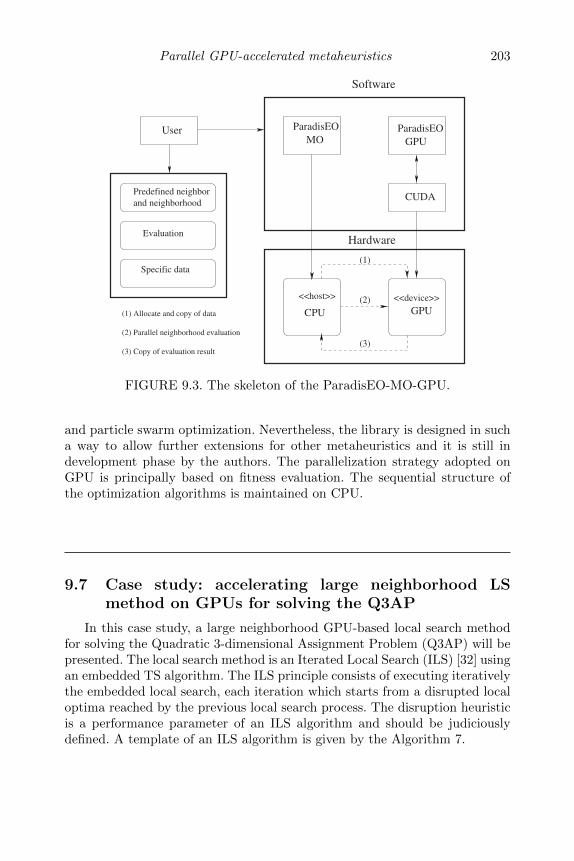
Parallel GPU-accelerated metaheuristics 203
UserMO
ParadisEO
GPU
ParadisEO
Software
Hardware
GPU
and neighborhood
Evaluation
Specific data
<<device>><<host>>
CUDA
(1)
(2)
(3)
(1) Allocate and copy of data
(2) Parallel neighborhood evaluation
(3) Copy of evaluation result
CPU
Predefined neighbor
FIGURE 9.3. The skeleton of the ParadisEO-MO-GPU.
and particle swarm optimization. Nevertheless, the library is designed in sucha way to allow further extensions for other metaheuristics and it is still indevelopment phase by the authors. The parallelization strategy adopted onGPU is principally based on fitness evaluation. The sequential structure ofthe optimization algorithms is maintained on CPU.
9.7 Case study: accelerating large neighborhood LSmethod on GPUs for solving the Q3AP
In this case study, a large neighborhood GPU-based local search methodfor solving the Quadratic 3-dimensional Assignment Problem (Q3AP) will bepresented. The local search method is an Iterated Local Search (ILS) [32] usingan embedded TS algorithm. The ILS principle consists of executing iterativelythe embedded local search, each iteration which starts from a disrupted localoptima reached by the previous local search process. The disruption heuristicis a performance parameter of an ILS algorithm and should be judiciouslydefined. A template of an ILS algorithm is given by the Algorithm 7.

204 Designing Scientific Applications on GPUs
Algorithm 7: iterated local search template
1 s0=GenerateInitSol();2 s∗=LocalSearch(s0);3 repeat4 s′=Perturbate(s∗, history);
5 s∗′=LocalSearch(s′);
6 s∗=AcceptationCriteria(s∗, s∗′, history);
7 until a maximum number of iterations is reached ;
9.7.1 The quadratic 3-dimensional assignment problem
The Q3AP is an extension of the well-known NP-hard QAP. The latteris one of the most studied problems by the combinatorial optimization com-munity due to its wide range of practical applications (site planning, sched-ule problem, computer-aided design, etc.) and to its computational challengessince it is considered as one of the most computationally difficult optimizationproblems.
The Q3AP was first introduced by William P. Pierskalla in 1967 [28] and,unlike the QAP, the Q3AP is a less studied problem. Indeed, the Q3AP wasrevisited only this past year and has recently been used to model some ad-vanced assignment problems such as the symbol-mapping problem encoun-tered in wireless communication systems and described in [13]. The Q3APoptimization problem can be mathematically expressed as follows:
min
n−1∑i=0
n−1∑j=0
n−1∑l=0
n−1∑k=0
n−1∑s=0
n−1∑r=0
cijlksrxijlxksr +
n−1∑i=0
n−1∑j=0
n−1∑l=0
bijlxijl
(9.1)
where
X = (xijl) ∈ I ∩ J ∩ L, (9.2)
xijl ∈ 0, 1, i, j, l = 0, 1, ..., n− 1 (9.3)
I, J , and L sets are defined as follows:
I = X = (xijl) :n−1∑j=0
n−1∑l=0
xijl = 1, i = 0, 1, ..., n− 1;
J = X = (xijl) :n−1∑i=0
n−1∑l=0
xijl = 1, j = 0, 1, ..., n− 1;

Parallel GPU-accelerated metaheuristics 205
L = X = (xijl) :n−1∑i=0
n−1∑j=0
xijl = 1, l = 0, 1, ..., n− 1
Other equivalent formulations of the Q3AP can be found in the literature.A particularly useful one is the permutation-based formulation wherein theQ3AP can be expressed as follows:
min
f(π1, π2) =
n−1∑i=0
n−1∑j=0
ciπ1(i)π2(i)jπ1(j)π2(j)+
n−1∑i=0
biπ1(i)π2(i)
(9.4)
where π1 and π2 are permutations over the set 0, 1, . . . , n− 1. According tothis formulation, minimizing the Q3AP consists of finding a double permuta-tion (π1, π2) which minimizes the objective function (9.4).
The Q3AP is proven to be an NP-hard problem since it is an extension ofthe quadratic assignment problem and of the axial 3-dimensional assignmentproblem which are both NP-hard problems. It is particularly computationallydifficult since the number of feasible solutions of an instance of size n is n!×n!.
9.7.2 Iterated tabu search algorithm for the Q3AP
To tackle large-sized instances of the Q3AP and speed up the search pro-cess, a parallel ILS algorithm has been designed. The local search embeddedin the ILS is a TS. A TS procedure [12] starts from an initial feasible solutionand tries, at each step, to move to a neighboring solution that minimizes thefitness (for a minimization case). If no such move exists, the neighbor solutionthat less degrades the fitness is chosen as a next move. This enables the TSprocess to escape local optima. However, this strategy may generate cycles,i.e., previous moves can be selected again. To avoid cycles, the TS managesa short-term memory that contains the moves that have been recently per-formed. A TS template is given by Algorithm 8.
Algorithm 8: tabu search template
1 GenerateInitSol(s0);2 TabuList=φ;3 t = 0;4 repeat5 m(t) = SelectBestMove(s(t));6 s(t+ 1) = ApplyMove(m(t), s(t));7 TabuList = TabuList
⋃m(t);
8 t = t+ 1;
9 until a maximum number of iterations is reached ;

206 Designing Scientific Applications on GPUs
9.7.3 Neighborhood functions for the Q3AP
The neighborhood function is a crucial parameter in any local search al-gorithm. Indeed, if the neighborhood function is not adequate to the problemand/or does not consider the targeted computing framework, any local searchalgorithm will fail to reach good quality solutions of the search space.
Regarding the Q3AP, many neighborhood structures can be considered. Abasic neighborhood was proposed and investigated in different works of theliterature [13,19] and consists of the set of all solutions (double-permutations)generated from the current one by an exchange of two positions in either thefirst (π1) or the second (π2) permutation. This neighborhood that we denoteby Nb can be formalized as follows:
Nb(π1, π2) = (π′
1, π′
2) : π′
1[k] = π1[l], π′
1[l] = π1[k]0 ≤ k 6= l < n;
π′
1[i] = π1[i], 0 ≤ i 6= k, l < n;
π′
2[j] = π2[j], 0 ≤ j < n⋃ (π
′
1, π′
2) : π′
2[k] = π2[l], π′
2[l] = π2[k]0 ≤ k 6= l < n;
π′
2[i] = π2[i], 0 ≤ i < n;
π′
1[j] = π1[j], 0 ≤ j 6= k, l < n
(9.5)
where (π1, π2) is the current solution and n is the size of the Q3AP instance.The size |Nb| of such neighborhood is equal to
|Nb| = n× (n− 1) (9.6)
In our GPU-based implementations, a large-sized neighborhood structurehas been used for experimentation. In fact, theoretical and experimental stud-ies have shown that the use of large neighborhood structures may improve theeffectiveness of LS algorithms [3]. However, for such a neighborhood, the gen-eration/evaluation step of an LS becomes a time-consuming task and maydramatically increase the computational time of the LS process. This justifiesthe use of intensive data-parallelism provided by GPUs where all neighboringsolutions may be concurrently evaluated.
The considered large-sized neighborhood consists of swapping two posi-tions in both permutations π1 and π2. This neighborhood structure, N(π1, π2),can be formalized as follows:

Parallel GPU-accelerated metaheuristics 207
N(π1, π2) = (π′
1, π′
2) : π′
1[k] = π1[l], π′
1[l] = π1[k],
π′
2[r] = π2[s], π′
2[s] = π2[r]0 ≤ k 6= l < n, 0 ≤ r 6= s < n;
π′
1[i] = π1[i], 0 ≤ i 6= k, l < n;
π′
2[j] = π′
2[j], 0 ≤ j 6= r, s < n
(9.7)
So, for a given Q3AP instance of size n, the size |N | of the advancedneighborhood set can be expressed by the following formula:
|N | =(n× (n− 1)
2
)2
(9.8)
9.7.4 Design and implementation of a GPU-based iteratedtabu search algorithm for the Q3AP
The use of GPU devices to speed up the search process of local searchmethods is not a straightforward task. It requires one to consider, at the sametime, the characteristics and underlying issues of the GPU architecture and theparallel models of LS methods. The main challenges that must be faced whendesigning a local search algorithm are the efficient distribution of the searchprocess between the CPU and the GPU minimizing the data transfer betweenthem, the hierarchical memory management and the capacity constraints ofGPU memories, and the thread synchronization. All these issues must beregarded when designing parallel LS models to allow solving of large scaleoptimization problems on GPU architectures.
To go back to our problem (i.e., Q3AP), we propose in Algorithm 9 an iter-ated tabu search on GPU (GPU-ITS). The parallel model is in agreement withthe iteration-level parallel model of LS methods presented in Section 9.3 (Fig.9.1). This algorithm can be seen as a cooperative model between the CPU andthe GPU. Indeed, the GPU is used as a coprocessor in a synchronous manner.The resource-consuming part, i.e., the generation and evaluation kernel, iscalculated by the GPU and the rest of the LS process is handled by the CPU.First of all, at initialization stage, memory allocations on GPU are made; theinput matrices (distance and flow matrices) and the initial candidate solutionof the Q3AP must be allocated (lines 4 and 5). Since GPUs require massivecomputations with predictable memory accesses, a structure has to be allo-cated for storing all the neighborhood fitnesses at different addresses (line 6).Second, the matrices and the initial candidate solution have to be copied onthe GPU (lines 7 and 8). We notice that the input matrices are read-onlystructures and do not change during all the execution of the LS algorithm.Therefore, their associated memory is copied only once during all the exe-cution. Third, comes the parallel iteration-level, in which each neighboringsolution is generated, evaluated, and copied into the neighborhood fitnesses

208 Designing Scientific Applications on GPUs
structure (from lines 10 to 14). Fourth, since the order in which candidateneighbors are evaluated is undefined, the neighborhood fitnesses structure hasto be copied to the host CPU (line 15). Then the selection strategy is appliedto this structure (line 16): the exploration of the neighborhood fitnesses struc-ture is done by the CPU. Finally, after a new candidate has been selected,this information is copied to the GPU (line 18). The process is repeated untila given number of iterations has been reached.
Algorithm 9: template of an iterated tabu search on GPU for solvingthe Q3AP
1 Choose an initial solution;2 Evaluate the solution;3 Initialize the tabu list;4 Allocate the Q3AP input data on GPU device memory;5 Allocate a solution on GPU device memory;6 Allocate a neighborhood fitnesses structure on GPU device memory;7 Copy the Q3AP input data on GPU device memory;8 Copy the solution on GPU device memory;9 t = 0;
10 repeat11 for each generated neighbor on GPU do12 Incremental evaluation of the candidate solution;13 Insert the resulting fitness into the neighborhood fitnesses
structure;
14 end15 Copy the neighborhood fitnesses structure on CPU host memory;16 Select the best admissible neighboring solution;17 Update the tabu list;18 Copy the chosen solution on GPU device memory;
19 until a maximum number of iterations is reached ;
9.7.5 Experimental results
In this section, some experimental results related to the approach presentedin Section 9.7.4 are reported. We recall that the approach is a GPU-based it-erated tabu search (GPU-ITS) method consisting in an iterated local search(ILS) embedding a tabu search (TS) and where the generation/evaluation stepof the TS process is executed on GPU. The ILS is used to improve the qualityof successive local optima provided by TS methods. This is achieved by per-turbing the local optima reached by the current TS process and reconsideringit as initial solution of the following TS process. Regarding our algorithm, theapplied perturbation is a random number µ of swaps in either the first or thesecond permutation where µ ∈ [2 : n] (n is the instance size).
Experiments have been carried out on a node of the Chirloute cluster ofthe Lille site. This is one of the 10 sites that currently make up Grid5000 [1],

Parallel GPU-accelerated metaheuristics 209
Instance Optimal Average Maximal Hits CPU GPU Speed- ITS/BKV1 value value time time up iter.
Nug12-d 580 615.4 744 35% 87.7 2.5 34.7× 1641.7 40.9 0.9 6.3
Nug13-d 1912 1985.4 2100 20% 209.2 3.3 63.5× 1751.0 1.3 1.0 5.6
Nug15-d 2230 2418.1 2580 30% 305.5 5.2 58.8× 17135.3 164.5 1.3 5.0
Nug18-d 17836 18110.2 18506 10% 1375.9 12.8 107.4× 19157.8 123.5 2.6 4.2
Nug22-d 42476 43282.1 44140 25% 4506.5 32.7 137.8× 18529.6 341.1 6.6 4.0
TABLE 9.1. Results of the GPU-based iterated tabu search for different Q3APinstances.
the French experimental computational grid. A Chirloute cluster node consistsof an Intel Xeon E5620 CPU and a NVIDIA Tesla Fermi M2050 (448 cores)GPU type. The number of ILS iterations and the number of TS iterationswere set respectively to 20 and 500. The tabu list size has been initalized tom4 , m being the size of the neighborhood set.
Table 9.1 reports the obtained results for the GPU-ITS using our large-sized neighborhood structure. The method has been tested on 5 Q3AP in-stances derived from the QAP Nugent instances in QAPLIB [6]. The averagetime measurement for 20 executions is reported in seconds and accelerationfactors compared to a standalone CPU are also considered. The algorithm isstopped when a maximum number of iterations has been reached or when theoptimal (or best known) value has been discovered. Average and max valuesof the evaluation function of the parallel GPU version have been measured.The number of successful tries (hits) and the average number of ILS iterationsto converge to the optimal/best known value are also represented. The associ-ated standard deviation for each average measurement is shown in small typecharacters.
Regarding the execution time, the generation and evaluation of the neigh-borhood in parallel on GPU provides an efficient way to speedup the searchprocess in comparison with a single CPU. In fact, for the smaller instanceNug12-d, the GPU version starts to be faster than the CPU one (accelerationfactor of 34.7 ×). As long as the problem size increases, the speedup growssignificantly (up to 137.8× for the Nug22-d instance). This means that the useof GPU provides an efficient way to deal with large neighborhoods. Indeed,the proposed neighborhoods were unpractical in terms of single CPU compu-tational resources for large Q3AP instances such as Nug22-d (estimated toaround 2 hours per run). So, implementing this algorithm on GPU has al-
1Best known value.

210 Designing Scientific Applications on GPUs
lowed the exploitation of parallelism in such neighborhood and improved therobustness/quality of provided solutions.
9.8 Conclusion
This chapter has presented state-of-the-art GPU-based parallel meta-heuristics and a case study on implementing large neighborhood local searchmethods on GPUs for solving large benchmarks of the quadratic three-dimensional assignment problem (Q3AP).
Implementing parallel metaheuristics on GPU architectures poses new is-sues and challenges such as memory management; finding efficient mappingstrategies between tasks to parallelize; and the GPU threads, thread diver-gence, and synchronization. Actually, most of metaheuristics have been im-plemented on GPU using different implementation strategies. In this chap-ter, a two-level classification of the reviewed works has been proposed: designlevel and implementation level. Design level regroups traditional parallel mod-els used for metaheuristics while implementation level refers to the way thosemodels are mapped to the GPU architecture. This classification focuses mainlyon the mapping between the metaheuristic tasks to parallelize and the GPUthreads. Indeed, the choice of a given mapping strategy strongly influencesthe other challenges (memory usage, communication, thread divergence).
Bibliography
[1] Grid’5000 French nation-wide grid. https://www.grid5000.fr.
[2] NVIDIA CUDA C Programming Best Practices Guide.http://docs.nvidia.com/cuda/cuda-c-best-practices-guide/.
[3] R. K. Ahuja, K. C. Jha, J. B. Orlin, and D. Sharma. Very large-scaleneighborhood search for the quadratic assignment problem. INFORMSJournal on Computing, 19(4):646–657, October 2007.
[4] M. G. Arenas, A. M. Mora, G. Romero, and P. A. Castillo. GPU compu-tation in bioinspired algorithms: A review. In Proceedings of the 11th In-ternational Conference on Artificial Neural Networks Conference on Ad-vances in Computational Intelligence, Volume Part I, IWANN’11, pages433–440, 2011.

Parallel GPU-accelerated metaheuristics 211
[5] C. Blum and A. Roli. Metaheuristics in combinatorial optimization:Overview and conceptual comparison. ACM Comput. Surv., 35:268–308,September 2003.
[6] R. E. Burkard, E. Cela, S. Karisch, and F. Rendl. QAPLIB - A quadraticassignment problem library.
[7] S. Cahon, N. Melab, and E.-G. Talbi. ParadisEO: A framework for thereusable design of parallel and distributed metaheuristics. Journal ofHeuristics, 10(3):357–380, 2004.
[8] A. Catala, J. Jaen, and J. A. Modioli. Strategies for accelerating antcolony optimization algorithms on graphical processing units. In IEEECongress on Evolutionary Computation, 2007. CEC 2007., pages 492–500. IEEE, 2007.
[9] J. M. Cecilia, J. M. Garcıa, A. Nisbet, M. Amos, and M. Ujaldon. En-hancing data parallelism for ant colony optimization on GPUs. Journalof Parallel and Distributed Computing, 73(1):42 – 51, 2013.
[10] A. Delevacq, P. Delisle, M. Gravel, and M. Krajecki. Parallel ant colonyoptimization on graphics processing units. Journal of Parallel and Dis-tributed Computing, 73(1):52 – 61, 2013.
[11] M. R. Garey and D. S. Johnson. Computers and Intractability: A Guideto the Theory of NP-Completeness. W. H. Freeman & Co., New York,NY, USA, 1990.
[12] F. Glover. Tabu search. ORSA Journal on Computing, 1(3):190 – 206,1989.
[13] P. M. Hahn, B. J. Kim, T. Stutzle, S. Kanthak, W. L. Hightower, Z. Ding,H. Samra, and M. Guignard. The quadratic three-dimensional assignmentproblem: Exact and approximate solution methods. European Journal ofOperational Research, 184:416–428, 2008.
[14] P. Hansen and N. Mladenovic. Variable neighborhood search. Computersand Operations Research, 24(11):1097 – 1100, 1997.
[15] A. Janiak, W. Janiak, and M. Lichtenstein. Tabu search on GPU. Journalof Universal Computer Science, 14(14):2416–2427, 2008.
[16] S. Kannan and R. Ganji. Porting AutoDock to CUDA. In IEEE Congresson Evolutionary Computation, CEC2010, 2010.
[17] S. Kirkpatrick, C. D. Gellat, and M. P. Vecchi. Optimization by simulatedannealing. Science, 220:671 – 680, 1983.

212 Designing Scientific Applications on GPUs
[18] J. M. Li, X. J. Wang, R. S. He, and Z. X. Chi. An efficient fine-grainedparallel genetic algorithm based on GPU-accelerated. In Proceedings ofthe 2007 IFIP International Conference on Network and Parallel Com-puting Workshops, NPC ’07, pages 855–862, Washington, DC, USA, 2007.IEEE Computer Society.
[19] L. Loukil, M. Mehdi, N. Melab, E.-G. Talbi, and P. Bouvry. Parallelhybrid genetic algorithms for solving Q3AP on computational grid. Int.J. Found. Comput. Sci., 23(2):483–500, 2012.
[20] T. V. Luong, N. Melab, and E-G. Talbi. Large neighborhood local searchoptimization on graphics processing units. In Workshop on Large-ScaleParallel Processing (LSPP) in Conjunction with the International Paral-lel & Distributed Processing Symposium (IPDPS), Atlanta, USA, 2010.
[21] T. V. Luong, N. Melab, and E.-G. Talbi. GPU-based multi-start localsearch algorithms. In Learning and Intelligent Optimization, volume 6683of Lecture Notes in Computer Science, pages 321–335. 2011.
[22] T. V. Luong, E. Taillard, N. Melab, and E-G. Talbi. Parallelizationstrategies for hybrid metaheuristics using a single GPU and multi-coreresources. In Parallel Problem Solving from Nature - PPSN XII, vol-ume 7492 of Lecture Notes in Computer Science, pages 368–377. SpringerBerlin Heidelberg, 2012.
[23] O. Maitre, L. Baumes, N. Lachiche, A. Corma, and P. Collet. Coarsegrain parallelization of evolutionary algorithms on GPGPU cards withEASEA. In Proceedings of the 11th Annual Conference on Genetic andEvolutionary Computation, GECCO ’09, pages 1403–1410, 2009.
[24] N. Melab, T. V. Luong, K. Boufaras, and E.-G. Talbi. TowardsParadisEO-MO-GPU: a framework for GPU-based local search meta-heuristics. In Advances in Computational Intelligence, volume 6691 ofLecture Notes in Computer Science, pages 401–408. 2011.
[25] Y. S. G. Nashed, R. Ugolotti, P. Mesejo, and S. Cagnoni. libCudaOpti-mize: An open source library of GPU-based metaheuristics. In Proceed-ings of the Fourteenth International Conference on Genetic and Evolu-tionary Computation Conference Companion, GECCO Companion ’12,pages 117–124, 2012.
[26] R. Nowotniak and J. Kucharski. GPU-based massively parallel implemen-tation of metaheuristic algorithms. Automatyka, 15(3):595–611, 2011.
[27] G. Paul. A GPU implementation of the simulated annealing heuristic forthe quadratic assignment problem. CoRR, abs/1208.2675, 2012.
[28] W. P. Pierskalla. The multi-dimensional assignment problem. TechnicalMemorandum No. 93, Operations Research Department, CASE Instituteof Technology, September 1967.

Parallel GPU-accelerated metaheuristics 213
[29] F. Pinel, B. Dorronsoro, and P. Bouvry. Solving very large instances ofthe scheduling of independent tasks problem on the GPU. Journal ofParallel and Distributed Computing, 73(1):101 – 110, 2012.
[30] P. Pospichal, J. Jaros, and J. Schwarz. Parallel genetic algorithm on theCUDA architecture. In Applications of Evolutionary Computation, vol-ume 6024 of Lecture Notes in Computer Science, pages 442–451. SpringerBerlin Heidelberg, 2010.
[31] N. Soca, J. L. Blengio, M. Pedemonte, and P. Ezzatti. PUGACE, acellular evolutionary algorithm framework on GPUs . In IEEE Congresson Evolutionary Computation (CEC), 2010.
[32] T. Stutzle. Iterated local search for the quadratic assignment problem.European Journal of Operational Research, 174(3):1519–1539, November2006.
[33] E. D. Taillard. FANT: Fast ant system. Technical report, 1998.
[34] E.-G. Talbi. Metaheuristics: From Design to Implementation. Wiley,2009.
[35] S. Tsutsui and N. Fujimoto. Solving quadratic assignment problems bygenetic algorithms with GPU computation: A Case Study. In Proceedingsof the 11th Annual Conference Companion on Genetic and Evolution-ary Computation Conference: Late Breaking Papers, GECCO ’09, pages2523–2530, 2009.
[36] S. Tsutsui and N. Fujimoto. ACO with tabu search on a GPU for solvingQAPs using move-cost adjusted thread assignment. In Proceedings ofthe 13th Annual Conference on Genetic and Evolutionary Computation,GECCO ’11, pages 1547–1554, 2011.
[37] P. Vidal and E. Alba. Cellular genetic algorithm on graphic processingunits. In Nature Inspired Cooperative Strategies for Optimization (NICSO2010), volume 284 of Studies in Computational Intelligence, pages 223–232. 2010.
[38] T. T. Wong and M. L. Wong. Parallel evolutionary algorithms onconsumer-level graphics processing unit. In Parallel Evolutionary Com-putations, volume 22 of Studies in Computational Intelligence, pages 133–155. 2006.
[39] Q. Yu, C. Chen, and Z. Pan. Parallel genetic algorithms on programmablegraphics hardware. In Advances in Natural Computation, volume 3612 ofLecture Notes in Computer Science, pages 1051–1059. 2005.

214 Designing Scientific Applications on GPUs
[40] Y. Zhou and Y. Tan. GPU-based parallel particle swarm optimization.In Proceedings of the Eleventh Conference on Congress on Evolution-ary Computation, CEC’09, pages 1493–1500, Piscataway, NJ, USA, 2009.IEEE Press.
[41] W. Zhu, J. Curry, and A. Marquez. SIMD tabu search for the quadraticassignment problem with graphics hardware acceleration. InternationalJournal of Production Research, 48(4):1035–1047, 2010.

Chapter 10
Linear programming on a GPU:a case study
Xavier Meyer and Bastien Chopard
Department of Computer Science, University of Geneva, Switzerland
Paul Albuquerque
Institute for Informatics and Telecommunications, HEPIA,University of Applied Sciences of Western Switzerland – Geneva, Switzerland
10.1 Introduction . . . . . . . . . . . . . . . . . . . . . . . . . . . . . . . . . . . . . . . . . . . . . . . . . . . . . . 21610.2 Simplex algorithm . . . . . . . . . . . . . . . . . . . . . . . . . . . . . . . . . . . . . . . . . . . . . . . . 217
10.2.1 Linear programming model . . . . . . . . . . . . . . . . . . . . . . . . . . . . . . 21710.2.2 Standard simplex algorithm . . . . . . . . . . . . . . . . . . . . . . . . . . . . . 21710.2.3 Revised simplex method . . . . . . . . . . . . . . . . . . . . . . . . . . . . . . . . . 21910.2.4 Heuristics and improvements . . . . . . . . . . . . . . . . . . . . . . . . . . . . 221
10.3 Branch-and-bound algorithm . . . . . . . . . . . . . . . . . . . . . . . . . . . . . . . . . . . . 22410.3.1 Integer linear programming . . . . . . . . . . . . . . . . . . . . . . . . . . . . . 22410.3.2 Branch-and-bound tree . . . . . . . . . . . . . . . . . . . . . . . . . . . . . . . . . . 22410.3.3 Branching strategy . . . . . . . . . . . . . . . . . . . . . . . . . . . . . . . . . . . . . . 22510.3.4 Node selection strategy . . . . . . . . . . . . . . . . . . . . . . . . . . . . . . . . . . 22610.3.5 Cutting-plane methods . . . . . . . . . . . . . . . . . . . . . . . . . . . . . . . . . . 227
10.4 CUDA considerations . . . . . . . . . . . . . . . . . . . . . . . . . . . . . . . . . . . . . . . . . . . . 22810.4.1 Parallel reduction . . . . . . . . . . . . . . . . . . . . . . . . . . . . . . . . . . . . . . . . 22810.4.2 Kernel optimization . . . . . . . . . . . . . . . . . . . . . . . . . . . . . . . . . . . . . 228
10.5 Implementations . . . . . . . . . . . . . . . . . . . . . . . . . . . . . . . . . . . . . . . . . . . . . . . . . 22910.5.1 Standard simplex . . . . . . . . . . . . . . . . . . . . . . . . . . . . . . . . . . . . . . . . 22910.5.2 Revised simplex . . . . . . . . . . . . . . . . . . . . . . . . . . . . . . . . . . . . . . . . . . 23210.5.3 Branch-and-bound . . . . . . . . . . . . . . . . . . . . . . . . . . . . . . . . . . . . . . . 236
10.6 Performance model . . . . . . . . . . . . . . . . . . . . . . . . . . . . . . . . . . . . . . . . . . . . . . . 23710.6.1 Levels of parallelism . . . . . . . . . . . . . . . . . . . . . . . . . . . . . . . . . . . . . 23810.6.2 Amount of work done by a thread . . . . . . . . . . . . . . . . . . . . . . 23810.6.3 Global performance model . . . . . . . . . . . . . . . . . . . . . . . . . . . . . . 23910.6.4 A kernel example: steepest-edge . . . . . . . . . . . . . . . . . . . . . . . . . 23910.6.5 Standard simplex GPU implementation model . . . . . . . . . 240
10.7 Measurements and analysis . . . . . . . . . . . . . . . . . . . . . . . . . . . . . . . . . . . . . . 24110.7.1 Performance model validation . . . . . . . . . . . . . . . . . . . . . . . . . . . 24110.7.2 Performance comparison of implementations . . . . . . . . . . . 241
215

216 Designing Scientific Applications on GPUs
10.8 Conclusion and perspectives . . . . . . . . . . . . . . . . . . . . . . . . . . . . . . . . . . . . . 245Bibliography . . . . . . . . . . . . . . . . . . . . . . . . . . . . . . . . . . . . . . . . . . . . . . . . . . . . . . 246
10.1 Introduction
The simplex method [4] is a well-known optimization algorithm for solvinglinear programming (LP) models in the field of operations research. It is partof software often employed by businesses for finding solutions to problemssuch as airline scheduling problems. The original standard simplex methodwas proposed by Dantzig in 1947. A more efficient method, named the re-vised simplex, was later developed. Nowadays its sequential implementationcan be found in almost all commercial LP solvers. But the always increasingcomplexity and size of LP problems from the industry, drives the demand formore computational power. In this context, parallelization is the natural ideato investigate [17]. Already in 1996, Thomadakis and Liu [23] implementedthe standard method on a massive parallel computer and obtained an increasein performances when solving dense or large problems.
A few years back, in order to meet the demand for processing power, graph-ics card vendors made their graphical processing units (GPU) available forgeneral-purpose computing. Since then GPUs have gained a lot of popularityas they offer an opportunity to accelerate algorithms having an architecturewell-adapted to the GPU model. The simplex method falls into this category.Indeed, GPUs exhibit a massive parallel architecture optimized for matrixprocessing. To our knowledge, there are only a few simplex implementationson GPU. Bieling et al. [10] presented encouraging results while solving smallto mid-sized LP problems with the revised simplex. However, the complexityof their algorithm seems to be rather close to the one of the standard simplexwith similar heuristics. Following the steps of this first work, an implementa-tion of the revised simplex [8] showed interesting results on dense and squarematrices. Furthermore, an implementation of the interior point method [18]outperformed its CPU equivalent on mid-sized problems.
The Branch-and-Bound (B&B) algorithm is extensively used for solving in-teger linear programming (ILP) problems. This tree-based exploration methodsubdivides the feasible region of the relaxed LP model into successively smallersubsets to obtain bounds on the objective value. Each corresponding submodelcan be solved with the simplex method, and the bounds computed determinewhether further branching is required. Hence, a natural parallelization of theB&B method is to let the CPU manage the B&B tree and dispatch the re-laxed submodels to an LP solver on a GPU. We refer the reader to Chapter 8,and the references therein, for a more complete introduction to parallel B&Balgorithms.
In this chapter, we present a GPU implementation of the standard andrevised simplex methods, based on the CUDA technology of NVIDIA. We also

Linear programming on a GPU: a case study 217
derive a performance model and establish its accurateness. Let us mention thatthere are many technicalities involved in CUDA programming, in particularregarding the management of tasks and memories on the GPU. Thus, finetuning is indispensable to avoid a breakdown on performance.
The chapter is organized as follows. First, we begin with a description ofthe standard and revised simplex methods and introduce the heuristics usedin our implementations. This is followed by a presentation of the B&B algo-rithm. The next section points out CUDA aspects which are important for ourimplementations. In the following one, we focus on the GPU implementationsof the simplex method as well as the B&B algorithm. In the sixth section, wedescribe a performance model for the standard simplex implementation. Inthe seventh section, a performance comparison between our implementationsis made on real-life problems and an analysis is given. Finally, we summarizethe results obtained and consider new perspectives.
10.2 Simplex algorithm
10.2.1 Linear programming model
An LP model in its canonical form can be expressed as the following op-timization problem:
maximize z = cTxsubject to Ax ≤ b
x ≥ 0(10.1)
where x = (xj), c = (cj) ∈ Rn,b = (bi) ∈ Rm, and A = (aij) is the m × nconstraints matrix. The objective function z = cTx is the inner product of thecost vector c and the unknown variables x. An element x is called a solutionwhich is said to be feasible if it satisfies the m linear constraints imposed byA and the bound b. The feasible region x ∈ Rn |Ax ≤ b, x ≥ 0 is a convexpolytope. An optimal solution to the LP problem will therefore reside on avertex of this polytope.
10.2.2 Standard simplex algorithm
The simplex method [4] is an algorithm for solving LP models. It pro-ceeds by iteratively visiting vertices on the boundary of the feasible region.This amounts to performing algebraic manipulations on the system of linearequations.
We begin by reformulating the model. So-called slack variables xn+i areadded to the canonical form in order to replace inequalities by equalities in

218 Designing Scientific Applications on GPUs
equation (10.1):
xn+i = bi−n∑j=1
aijxj (i = 1, 2, ...,m) (10.2)
The resulting problem is called the augmented form in which the variables aredivided into two disjoint index sets, B and N , which correspond to the basicand nonbasic variables. Basic variables, which form the basis of the problem,are on the left-hand side of equation (10.2), while nonbasic variables, whichform the core of the equations, appear on the right-hand side. We can thusconsider the following LP form:
maximize z = cTxsubject to Ax = b
x ≥ 0(10.3)
where x ∈ Rn+m and A is now the m× (n+m) matrix obtained by concate-nating the constraints matrix with the m ×m identity matrix Im. The costvector has been padded with zeros so that c ∈ Rn+m.
The basic and nonbasic variables can be separated given the expressionANxN + xB = b. Similarly, z = cTx = cTNxN + cTBxB with cB = 0. By def-inition, a basic solution is obtained by assigning null values to all nonbasicvariables (xN = 0). Hence, x = xB = b is a basic solution.
The simplex algorithm searches for the optimal solution through an itera-tive process. For the sake of simplicity, we will assume here that b > 0, thatis, the origin belongs to the feasible region. Otherwise a preliminary treatmentis required to generate a feasible initial solution (see Section 10.2.4). A typicaliteration then consists of three operations (summarized in Algorithm 10).
1. Choosing the entering variable. The entering variable is a nonba-sic variable whose increase will lead to an increase in the value of theobjective function z. This variable must be selected with care so as toyield a substantial leap towards the optimal solution. The standard wayof making this choice is to select the variable xe with the largest pos-itive coefficient ce = maxcj > 0 | j ∈ N in the objective function z.However, other strategies, such as choosing the positive coefficient withthe smallest index, also prove to be useful.
2. Choosing the leaving variable. This variable is the basic variablewhich first violates its constraint as the entering variable xe increases.The choice of the leaving variable must guarantee that the solution re-mains feasible. More precisely, setting all nonbasic variables except xeto zero, xe is bounded by
t = min
biaie
∣∣∣∣ aie > 0, i = 1, . . . ,m

Linear programming on a GPU: a case study 219
If t = +∞, the LP problem is unbounded.
Otherwise, t =b`a`e
for some ` ∈ B, and x` is the leaving variable;
the element a`e is called the pivot.
3. Pivoting. Once both variables are defined, the pivoting operationswitches these variables from one set to the other: the entering variableenters the basis B, taking the place of the leaving variable which nowbelongs to N , namely, B ← (B \ `) ∪ e and N ← (N \ e) ∪ `.Correspondingly, the columns with index ` and e are exchanged be-tween Im and AN , and similarly for cB = 0 and cN . We then updatethe constraints matrix A, the bound b and the cost c using Gaussianelimination. More precisely, denoting Im, AN , cB, and cN as the result-ing elements after the exchange, Gaussian elimination then transformsthe tableau
AN Im b
cTN cTB z
into a tableau with updated values for AN , cN , and b
AN Im b
cTN cTB z − tce
The latter is obtained by first dividing the `-th row by a`e; the resultingrow multiplied by aie (i 6= `) is then subtracted to the ith row; the sameoperation is performed using ce and the last row. Hence, cB = 0. Theseoperations amount to jumping from the current vertex to an adjacentvertex with objective value z = tce.
The algorithm ends when no more entering variable can be found, that is,when cN ≤ 0.
10.2.3 Revised simplex method
The operation that takes the most time in the standard method is thepivoting operation, and more specifically, the update of the constraints ma-trix A. The revised method tries to avoid this costly operation by updatingonly a smaller part of this matrix.
The revised simplex method uses the same operations as in the standardmethod to choose the entering and leaving variables. However, since the con-straints matrix A need not be fully updated, some additional reformulationis required.
At any stage of the algorithm, basic and nonbasic variables can be sep-arated according to Ax = ANxN + ABxB = b. We can then transform the

220 Designing Scientific Applications on GPUs
Algorithm 10: standard simplex algorithm
1 //1. Find entering variable;2 if cN ≤ 0 then3 return Optimal;4 end5 Choose an index e ∈ N such that ce > 0 ;6 //2. Find leaving variable;7 if (AN )e≤ 0 then8 return Unbounded9 end
10 Let ` ∈ B be the index such that ;
11 t :=b`a`e
= min
biaie
∣∣∣∣ aie > 0, i = 1, . . . ,m
;
12 //3. Pivoting, update ;13 B := (B \ `) ∪ e, N := (N \ e) ∪ `;14 Compute zbest := zbest + tce;15 Exchange (Im)` and (AN )e, (cB)` and (cN )e;16 Update AN , cN and b;17 Go to 1.;
system Ax = b into ABxB = b−ANxN . Let us denote B = AB,N = AN .Since B is invertible, we can write
xB = B−1b−B−1NxN
z = cTBB−1b + (cTN − cTBB−1N)xN
The vector cTN − cTBB−1N is called the reduced cost vector.The choice of the leaving variable can be rewritten. Setting all nonbasic
variables except the entering variable xe to zero, xe is then bounded by
t = min
(B−1b)i
(B−1N)ie
∣∣∣∣ (B−1N)ie > 0, i = 1, . . . ,m
If t = +∞, the LP problem is unbounded. Otherwise, t = (B−1b)`(B−1N)`e
for some
` ∈ B, and x` is the leaving variable.Recall that the pivoting operation begins by exchanging columns with
index ` and e between B and N and similarly for cB and cN .To emphasize the difference between standard and revised simplex, we first
express the updating for the standard simplex. This amounts to
[B N b]← [Im B−1N B−1b]
[cTB cTN ]← [0 cTN − cTBB−1N]

Linear programming on a GPU: a case study 221
which moves the current vertex to an adjacent vertex x = B−1b with objectivevalue z = cTBB−1b (the end condition remains cN ≤ 0). Many computationsperformed in this update phase can in fact be avoided.
The main point of the revised simplex method is that the only values whichreally need to be computed at each step are B−1, B−1b, B−1Ne, cTBB−1, andcTBB−1b. However, matrix inversion is a time-consuming operation (of cubicorder for Gaussian elimination). Fortunately, there are efficient ways of com-puting an update for B−1. One way is to take advantage of the sparsity of theLP problem by using the so-called LU decomposition1 for sparse matrices [3].This decomposition may be updated at a small cost at each iteration [22].Another way is to use the product form of the inverse [6], which we describehereafter.
Let b1, . . . ,bm be the columns of B, v ∈ Rm, and a = Bv =∑mi=1 vibi.
Denote Ba = (b1, . . . ,bp−1,a,bp+1, . . . ,bm) for a given 1 ≤ p ≤ m such thatvp 6= 0. We want to compute Ba
−1. We first write
bp =1
vp+ a
∑i 6=p
−vivp
bi
Define
η =
(−v1
vp, . . . ,
−vp−1
vp,
1
vp,−vp+1
vp, . . . ,
−vmvp
)Tand
E = (ε1, . . . , εp−1,η, εp+1, . . . , εm)
where εj = (0, . . . , 0, 1, 0, . . . , 0)T is the jth element of the canonical basisof Rm. Then BaE = B, so Ba
−1 = E B−1.We apply these preliminary considerations to the simplex algorithm with
a = Ne,v = (B−1N)e (recall that xe is the entering variable). If initially B isthe identity matrix Im, at the kth iteration of the algorithm, the inverse matrixis given by B−1 = EkEk−1 · · ·E2E1, where Ei is the matrix constructed atthe ith iteration.
10.2.4 Heuristics and improvements
Specific heuristics or methods are needed to improve the performance andstability of the simplex algorithm. We will explain below how we find an initialfeasible solution and how we choose the entering and leaving variables.
Finding an initial feasible solution
Our implementations use the two-phase simplex [4]. The first phase aimsat finding a feasible solution required by the second phase to solve the origi-nal problem. If the origin x = 0 is not a feasible solution, we proceed to find
1The LU decomposition is a linear algebra decomposition which allows to write a matrixas a product of a lower and an upper triangular matrix.
222 Designing Scientific Applications on GPUs
such a solution by solving a so-called auxiliary problem with the simplex al-gorithm. This can be achieved by adding a nonnegative artificial variable toeach constraint equation corresponding to a basic variable which violates itsnonnegativity condition, before minimizing the sum of these artificial vari-ables. The algorithm will thus try to drive all artificial variables towards zero.If it succeeds, then a basic feasible solution is available as an initial solutionfor the second phase in which it attempts to find an optimal solution to theoriginal problem. Otherwise, the problem is infeasible.
To avoid having to introduce these additional auxiliary variables, we usean alternate version of this procedure. For basic variables with index in I =j ∈ B | xj < 0, we temporarily relax the nonnegativity condition in order tohave a feasible problem and then apply the simplex algorithm to minimize w =−∑j∈I xj . However, we update I at each iteration and modify accordingly
the objective function, whose role is to drive these infeasible basic variablestowards their original bound. If at some stage I = ∅, we end up with aninitial feasible solution. Otherwise, the algorithm terminates with I 6= ∅ andw > 0, which indicates that the original problem is infeasible. The alterationintroduced above involves more computations during the first phase, but itoffers the advantage of preserving the problem size and making good use ofthe GPU processing power.
Choice of the entering variable
The number of iterations required to solve a problem depends on themethod used to select the entering variable. The one described in Sec-tion 10.2.2 chooses the most promising variable xe in terms of cost. Whilebeing inexpensive to compute, this method can lead to an important numberof iterations before the best solution is found.
There exist various heuristics to select this variable xe. One of the mostcommonly used is the steepest-edge method [15]. To improve the speed atwhich the best solution is found, this method takes into account the coefficientsof B−1N. This can be explained from the geometrical point of view. Theconstraints Ax = b form the hull of a convex polytope. The simplex algorithmmoves from one vertex (i.e., a solution) to another while trying to improvethe objective function. The steepest-edge method searches for the edge alongwhich the rate of improvement of the objective function is the best. Theentering variable xe is then determined by
e = arg max
cj√γj
∣∣∣∣ cj > 0, j ∈ N
with γj = ‖B−1Nj‖2.This method is quite costly to compute but it reduces significantly the
number of iterations required to solve a problem. This heuristic can be directlyapplied to the standard simplex since the full tableau is updated at eachiteration. However, it defeats the purpose of the revised simplex algorithm

Linear programming on a GPU: a case study 223
since the aim is precisely to avoid updating the whole constraints matrix ateach iteration. Taking this into account, the steepest-edge coefficients γ areupdated based only on their current value. For the sake of clarity, the hatnotation is used to differentiate the next iteration value of a variable from itscurrent value: for example if γ denotes the steepest-edge coefficients at thecurrent iteration, then γ are the updated coefficients.
Given the column of the entering variable d = (B−1N)e, we may processafresh the steepest-edge coefficient of the entering variable as γe = ‖d‖2. Theupdated steepest-edge coefficients are then given by
γj = maxγj − 2αjβj + γeαj
2, 1 + αj2
for j 6= e
γe = γe/d2e
with α = NT((B−1)T)` and β = NT(B−1)Td
Choice of the leaving variable
The stability and robustness of the algorithm depend considerably on thechoice of the leaving variable. With respect to this, the expand method [13]proves to be very useful in the sense that it helps to avoid cycles and re-duces the risks of encountering numerical instabilities. This method consistsof two steps of complexity O(m). In the first step, a small perturbation is ap-plied to the bounds of the variables to prevent stalling of the objective value,thus avoiding cycles. These perturbed bounds are then used to determine thegreatest gain on the entering variable imposed by the most constraining basicvariable. The second phase uses the original bounds to define the basic vari-able offering the gain closest to the one of the first phase. This variable willthen be selected for leaving the basis.

224 Designing Scientific Applications on GPUs
10.3 Branch-and-bound algorithm
10.3.1 Integer linear programming
In some problems, variables are integer-valued. For example, in a vehiclerouting problem, one cannot assign one third of a vehicule to a specific route.ILP problems restrict LP problems by imposing an integrality condition onthe variables. While this change may seem to have little impact on the model,the aftermaths on the resolution method are quite important.
From a geometrical perspective, the simplex algorithm is a method forfinding an optimum in a convex polytope defined by an LP problem. How-ever, the additional integrality condition results in the loss of this convexityproperty. The resolution method must then be altered in order to find a so-lution to the ILP problem. The idea is to explore the solution space by adivide-and-conquer approach in which the simplex algorithm is used to find alocal optimum in subspaces.
10.3.2 Branch-and-bound tree
The solution space is explored by the B&B algorithm [1]. The strategyused is conceptually close to a tree traversal.
At first, the ILP problem is considered as an LP problem by relaxing theintegrality condition before applying an LP solver to it. This initial relaxedproblem represents the root of the tree about to be built. From the obtainedsolution ξ, if ξj is not integral for some j, then xj can be chosen as a branch-ing variable. The current problem will then be divided, if possible, into twosubproblems: one having xj ≤ bξjc and the other xj ≥ dξje. Each of these LPsubproblems represents a child node waiting to be solved.
This is repeated for each subproblem in such a way that all variables are ledtowards integral values. At some point a subproblem will either be infeasibleor lead to a feasible ILP solution (leaf nodes). The algorithm ends when thetree has been fully visited, returning the best feasible ILP solution.
During the exploration, lower and upper bounds on the objective valueare computed. The upper bound is represented by the best objective valueencountered in a child node. This nonadmissible solution hints towards whatthe objective value of the ILP problem could be. The lower bound is thebest ILP solution yet found, in other words the objective value of the mostpromising leaf node. The bounds may be used to prune subtrees when furtherbranching cannot improve the best current solution.
In the B&B algorithm, the main two operations that impact the conver-gence of the bounds towards the optimal solution are the branching strategyand the node selection strategy.

Linear programming on a GPU: a case study 225
Example
Figure 10.1 illustrates the use of the B&B algorithm for solving an ILP.The ILP problem is the following:
Maximize z = x1 + 4x2
Subject to 5x1 + 8x2 ≤ 40
−2x1 + 3x2 ≤ 9
x1, x2 ≥ 0 integer-valued
The nodes are solved with the simplex method in the order written on thefigure. At the 3rd step of the B&B, the first feasible solution is encountered(light grey leaf). The optimal solution is encountered at the 7th step (darkgrey leaf). However, this is assessed only after solving the last two nodes (8thand 9th) whose objective value z is inferior to the best one yet found.
FIGURE 10.1. Solving an ILP problem using a branch-and-bound algorithm.
10.3.3 Branching strategy
The branching strategy defines the method used to select the variable onwhich branching will occur. The objective value of the child node dependsgreatly on the choice of this variable. Branching on a variable may lead to adrop on the upper bound and thus speed up the exploration, while branchingon other variables could leave this bound unchanged.

226 Designing Scientific Applications on GPUs
Several branching strategies exist [19]. Let us briefly comment on some ofthem in terms of improving the objective function and processing cost.
• Smallest-index strategy is a greedy approach that always selects the vari-able with the smallest index as branching variable. This method is sim-ple, has a cheap processing cost, but does not try to select the bestvariable.
• Strong branching strategy is an exhaustive strategy. The branching vari-able selected is the one among all the potential variables that leads tothe best solution. This means that for each potential branching vari-able, its potential child nodes must be solved. This method is easy toimplement, but its computational cost makes it inefficient.
• Reliability branching strategy is a strategy which maintains a pseudo-cost [12] for each potential branching variable. The pseudocost of a vari-able is based on the result obtained when branching on it at previoussteps. Since at the start, pseudocosts are unreliable, a limited strongbranching approach is used until pseudocosts are deemed reliable. Thismethod is more complex than the two others and requires fine tuning.It offers, however, the best trade-off between improvement and com-putional cost.
10.3.4 Node selection strategy
The node selection strategy defines the methodology used to explore thetree. While the usual depth-first search and breadth-first search are consideredand used, some remarks about the tree exploration must be made. First letus mention a few facts:
1. Solutions obtained from child nodes cannot be better than the one oftheir parent node.
2. An LP solver is able to quickly find a solution if the subproblem (childnode) is only slightly different from its parent.
Given the above statements, it is of interest to quickly find a feasible solution.Indeed, this allows the pruning of all pending nodes which do not improve thesolution found. However, the quality of the latter solution impacts the amountof nodes pruned. It takes more time to produce a good solution because onemust search for the best nodes in the tree. Consequently, a trade-off must bemade between the quality and the time required to find a solution.
Two types of strategies [21] can then be considered:
• Depth-first search aims at always selecting one of the child nodes until aleaf (infeasible subproblem or feasible solution) is reached. This strategyis characterized by fast solving, and it quickly finds a feasible solution.It mostly improves the lower bound.

Linear programming on a GPU: a case study 227
• Best-first search aims at always selecting one of the most promisingnodes in the tree. This strategy is characterized by slower solving butguarantees that the first feasible solution found is the optimal. It mostlyimproves the upper bound.
A problem occurs with the best-first search strategy: there might be numer-ous nodes having solutions of the same quality, thus making the choice of anode difficult. To avoid this problem, the best-estimate search strategy [14]differentiates the best nodes by estimating their potential cost with the helpof a pseudocost (see previous section).
The most promising variant is a hybrid strategy in which the base strategyis the best-estimate search with the subtrees of the best-estimated nodes beingthen subject to a limited depth-first search, more commonly called plunging.This method launches a fast search for a feasible solution in the most promisingsubtrees, thus improving the upper and lower bounds at the same time.
10.3.5 Cutting-plane methods
Cutting-planes [25] (also simply cuts) are new constraints whose role isto cut off parts of the search space. They may be generated from the firstLP solution (cut-and-branch) or periodically during the B&B (branch-and-cut). On the one hand cutting-planes may considerably reduce the size of thesolution space, but on the other hand they increase the problem size. Moreover,generating cutting-planes is costly since it requires a thorough analysis of thecurrent state of the problem.
Various types or families of cutting-planes exist. Those that are most ap-plied are the Gomory cutting-planes and the complemented mixed integerrounding inequalities (c-MIR). Other kinds of cutting-planes target specificfamilies of problems, for example, the 0-1 knapsack cutting-planes or flowcover cuts.
The cutting-planes generated must be carefully selected in order to avoida huge increase in the problem size. They are selected according to threecriteria: their efficiency, their orthogonality with respect to other cutting-planes, and their parallelism with respect to the objective function. Cutting-planes having the most impact on the problem are then selected, while theothers are dropped.

228 Designing Scientific Applications on GPUs
10.4 CUDA considerations
The most expensive operations in the simplex algorithm are linear algebrafunctions. The NVIDIA CUDA Basic Linear Algebra Subroutines2 (CUBLAS)library is a GPU-accelerated version of the complete standard BLAS library.It can be used for dense matrix-vector multiplications (cublasDgemv) anddense vector sums (cublasDaxpy). The CUSPARSE library is used for thesparse matrix-vector multiplication (cusparseDcsrmv).
However, complex operations are required to implement the simplex andmust be coded from scratch. For example, reduction operations, such asargmax or argmin, are fundamental for selecting variables. In the followingsection, we first quickly describe the CUDA reduction operation, before mak-ing some global remarks on kernel optimization.
10.4.1 Parallel reduction
A parallel reduction operation is performed in an efficient manner insidea GPU block as shown in Figure 10.2. Shared memory is used for a fast andreliable way to communicate between threads. However, at the grid level, re-duction cannot be easily implemented due to the lack of direct communicationbetween blocks. The usual way of dealing with this type of limitation is toapply the reduction in two separate steps. The first one involves a GPU kernelreducing the data over multiple blocks, the local result of each block beingstored on completion. The second step finishes the reduction on a single blockor on the CPU. An optimized way of doing the reduction can be found in theexamples3 provided by NVIDIA.
10.4.2 Kernel optimization
Optimizing a kernel is a difficult task. The most important point is todetermine whether the performances are limited by the bandwidth or by theinstruction throughput. Depending on the case and the specificities of theproblem, various strategies may be applied. This part requires a good un-derstanding of the underlying architecture and its limitations. The CUDAProgramming Guide offers some insight into this subject, as do the interestingarticles and presentations by Vassily Volkov [24]. The CUDA profiler is thebest way to monitor the performances of a kernel. This tool proposes multipleperformance markers giving indications about potential bottlenecks.
2The libraries CUBLAS and CUSPARSE are available athttps://developer.nvidia.com/cublas and https://developer.nvidia.com/cusparse.
3Available at http://docs.nvidia.com/cuda/cuda-samples/index.html#advanced

Linear programming on a GPU: a case study 229
10 1 8 -1 0 -2 3 5 -2 -3 2 7 0 11 20
-2 -3 2 7 0 11 20
-2 -3 2 7 0 11 20
-2 -3 2 7 0 11 20
-2 -3 2 7 0 11 20
-2 -3 2 7 0 11 20
8 -2 10 6 0 9 3 7
0 9 3 7
0 9 3 7
1313
13 13
0 9 3 71313
8 7
21 20
2041
FIGURE 10.2. Example of a parallel reduction at block level. (CourtesyNVIDIA).
10.5 Implementations
In this section, the implementations of the simplex algorithm are studied.The emphasis is put on the main algorithms and kernels having a major impacton performance. The expand method used for choosing the leaving variablewill not be detailed for that reason. Then the B&B implementation is quicklyexplained focusing on the interaction between the B&B algorithm and thesimplex solver.
10.5.1 Standard simplex
The implementation of the standard simplex algorithm (see Section 10.2.2)is rather straightforward. The main difference with Algorithm 10 is that thebasis matrix is not stored in memory since it is equal to the identity matrixmost of the time. Instead a proper data structure keeps track of the basicvariables and their values.
The first step of Algorithm 11 is the selection of the entering variable us-ing the steepest-edge heuristic. This step is discussed thoroughly in the nextsection. Then the leaving variable index ` and the potential gain on the enter-ing variable t are determined using the expand method. Finally, the pivotingis done. The nonbasic matrix AN and the objective function coefficients care updated using the CUBLAS library (respectively, with cublasDger andcublasDaxpy). This requires the entering variable column d and the leavingvariable row r to be copied and slightly altered. The new value of the variables

230 Designing Scientific Applications on GPUs
Algorithm 11: standard simplex algorithm
1 // Find entering variable xe;2 γj ← ‖(AN )j‖2;
3 e← argmax(c/√γ);
4 if e < 0 then5 return optima found6 end7 // Find leaving variable x`;8 `, t← expand((AN )e);9 if ` < 0 then
10 return unbounded11 end12 // Pivoting ;13 d← (AN )e , de ← (AN )`e − 1;
14 r← NT`;
15 xe ← xe + t;16 xB ← xB − t(AN )e;
17 AN ← AN − dTr/(AN )`e // cublasDger ;18 c← c− c`r/(AN )`e // cublasDaxpy ;19 swap(xe, x`);
is computed and, since we use a special structure instead of the basis matrix,the entering and leaving variables are swapped.
Choice of the entering variable
Let us discuss two different approaches for the selection of the enteringvariable. The first one relies on the CUBLAS library. The idea is to split thisstep into several small operations, starting with the computation of the normsone by one with the cublasDnrm2 function. The score of each variable is thenobtained by dividing the cost vector c by the norms previously computed. Theentering variable is finally selected by taking the variable with the biggeststeepest-edge coefficient using cublasDamax.
While being easy to implement, such an approach would lead to poorperformances. The main problem is a misuse of data parallelism. Each columncan be processed independently, and thus at the same time. Moreover, slicingthis step into small operations requires that each temporary result be storedin global memory. This creates a huge amount of slow data transfers betweenkernels and global memory.
Listing 10.1. a kernel for the choice of the entering variable
extern s h a r e d volat i le double sData [ ] ;g l o b a l void
s e l e c t InVar ( int m, int n , double ∗c , double ∗AN, u int pitchAN ,u int ∗ res Idx , double ∗ resVal )

Linear programming on a GPU: a case study 231
5 uint i , maxIdx = −1, bid = blockIdx . x ;double val , locSum , xScore , maxScore = 0 . 0 ;while ( bid < n) // Processing multiple columns
i = threadIdx . x ;locSum = 0 . 0 ;
10 i f ( i sPotent i a lEnte r ingVar ( bid ) ) // Do the local processingwhile ( i < m) // Each thread processes multiple elements
va l = AN[ i+bid ∗pitchAN ] ;locSum += val ∗ va l ;i += blockDim . x ;
15 // Reduce the value using shared memoryreduceSum ( locSum ) ;i f ( t i d == 0) // Is this the best variable encountered ?
// on tid=0 locSum equals the steepest edge coeffc ient20 xScore = cVal∗ r s q r t ( locSum ) ;
i f ( fabs ( maxScore ) < f abs ( xScore ) ) maxIdx = bid ;maxScore = xScore ;
25
sync th r ead s ( ) ;bid += gridDim . x ;
30 // Write the result into global memory
i f ( t i d == 0) r e s Idx [ b lockIdx . x ] = maxIdx ;resVal [ b lockIdx . x ] = maxScore ;
35
To avoid this, the whole step could be implemented as a unique kernel, asshown in the simplified Listing 10.1. Each block evaluates multiple potentialentering variables. The threads of a block process part of the norm of a column.Then a reduction (see Section 10.4.1) is done inside the block to form the fullnorm. The thread having the final value can then compute the score of thecurrent variable and determine if it is the best one encountered in this block.Once a block has evaluated its variables, the most promising one is stored inglobal memory. The final reduction step is finally done on the CPU.
The dimension of the blocks and grid have to be chosen wisely as a functionof the problem size. The block size is directly correlated to the size of a columnwhile the grid size is a trade-off between giving enough work to the schedulerin order to hide the latency and returning as few potential entering variablesas possible for the final reduction step.
CPU-GPU interactions
The bulk of the data representing the problem is stored on the GPU. Onlyvariables required for decision-making operations are updated on the CPU.The communications arising from the aforementioned scheme are illustrated inFigure 10.3. The amount of data exchanged at each iteration is independent ofthe problem size ensuring that this implementation scales well as the problemsize increases.

232 Designing Scientific Applications on GPUs
CPU GPU
Select EnteringVariable
Select LeavingVariable
Pivoting & Swap
SE Kernel
Expand Kernel
cublasDger
cubasAxpy
Prepare d, r
Swaps
e < 0 ?
l < 0 ? Unbounded or Infeasible
Found Optimal
e
yesno
yesno
e
l,t
e,l,t
FIGURE 10.3. Communications between CPU and GPU.
10.5.2 Revised simplex
The main steps found in the previous implementation are again presentin the revised simplex. The difference comes from the fact that a full updateof the matrix N is not necessary at every iteration. As explained in Sec-tion 10.2.3, the basis matrix B is updated so that the required values, such asthe entering variable column, can be processed from the now constant matrixN. Due to these changes, the steepest-edge method is adapted. The resultingimplementation requires more operations as described in Algorithm 12.
Let us compare the complexity, in terms of level 2 and level 3 BLAS op-erations, of both implementations. The standard one has mainly two costlysteps: the selection of the entering variable and the update of the matrix N.These are level 2 BLAS operations or the equivalent, and thus the approximatecomplexity is O(2mn).
The new implementation proposed has three operations cublasDgemvwhere the matrix N is involved, and three others with the matrix B−1. Thecomplexities of these operations are respectively O(mn) and O(m2). The up-date of the matrix B is a level 3 BLAS operation costing O(m3). The approx-imate complexity is then O(3mn+ 3m2 +m3).
It appears clearly that, in the current state, the revised simplex imple-mentation is less efficient than the standard one. However this method canbe improved and might well be better than the standard one based on twocharacteristics of LP problems: their high sparsity and the fact that usuallym n. In the next sections, we will give details about these improvements.

Linear programming on a GPU: a case study 233
Algorithm 12: revised simplex algorithm
1 // Find entering variable xe, e ∈ B;
2 τ ← (B−1)TcB // cublasDgemv ;
3 υ ← cN −NTτ // cublasDgemv ;
4 e← argmax(υ/√γ);
5 if e < 0 then6 return optima found7 end8 // Find leaving variable x`, ` ∈ N ;9 d← B−1Ne // cublasDgemv ;
10 `, t← expand(d);11 if ` < 0 then12 return unbounded13 end14 // Pivoting, basis update;
15 κ← (B−1)Td // cublasDgemv ;
16 β ← NTκ // cublasDgemv ;17 B−1 ← E B−1;18 xe ← xe + t;19 xB ← xB − td;20 swap(x`, xe);
21 α← NT((B−1)T
)`
// cublasDgemv ;
22 γe ← ‖d‖2 ;
23 γj ← maxγj − 2αjβj + γeαj
2, 1 + αj2, ∀j 6= e, γe ← γe/d
2e;

234 Designing Scientific Applications on GPUs
Choice of the entering variable
Once again, this part of the algorithm can be substantially improved. First,algorithmic optimizations must be considered. Since row α of the leavingvariable is processed to update the steepest-edge coefficients, the cost vectorυ can be updated directly without using the basis matrix B. This is done asfollow
υj = υj − υeαj , ∀j 6= e, υe = − υeαe
where υj denotes the value of υj at the previous iteration. It is important tonote that all these updated values (υ,γ) must be processed afresh once in awhile to reduce numerical errors.
Including this change, the operations required for the selection of the en-tering variable e are detailed in Algorithm 13. The values related to the en-tering variable at the previous iteration e = q are used. The reduced costsare updated, followed by the steepest-edge coefficients. With these values theentering variable is determined.
Algorithm 13: choice of the entering variable
1 q ← e;
2 υq ← cq − cTB d ;3 γq ← ‖d‖;4 // Update of the reduced costs;5 υj ← υj − αj υq, ∀j 6= q;
6 υq ←υqd2q
;
7 // Update of the steepest edge coefficients;
8 γj ← maxγj − 2αj βj + γqα
2j , 1 + α2
j
, ∀j 6= q;
9 γq ← γq/d2q ;
10 // Selection of the entering variable;
11 e← argmax(υ/√γ);
Coupling these operations into a single kernel is quite beneficial. This leadsυ and γ to be loaded only once from global memory. Their updated values arestored while the entering variable e is selected. With these changes, the globalcomplexity of this step is reduced from O(mn+m2 +n) to O(n). Moreover theremaining processing is done optimally by reusing data and by overlappingglobal memory access and computations.
Basis update
The basis update B−1 ← E B−1 is a matrix-matrix multiplication. How-ever, due to the special form of the matrix E (see Section 10.2.3), the complex-ity of this operation can be reduced from O(m3) to O(m2) [10]. The matrix

Linear programming on a GPU: a case study 235
E is merely the identity matrix having the `th column replaced by the vectorη. The update of the matrix B−1 can be rewritten as
B−1ij = B−1
ij
(1− di
d`
), ∀i 6= `, B−1
`j =B−1`j
d`
As shown in Listing 10.2, each block of the kernel processes a single columnwhile each thread may compute multiple elements of a column. This organi-zation ensures that global memory accesses are coalescent since the matrix Bis stored column-wise.
Listing 10.2. basis update
extern s h a r e d volat i le double sdata [ ] ;g l o b a l void
updateBasisKernel ( int m, uint l , double d l , double ∗B,u int pitch B , double ∗d)
5 uint bId = blockIdx . x , t Id = threadIdx . x ;u int c o l S t a r t = bId∗ pitch B ;double Bij , d i , B2 i j ;
// First thread loads Blj so i t can be10 // broadcast via shared memory to each thread
i f ( t Id == 0)sdata [ 0 ] = B[ c o l S t a r t+l ] / d l ;
s ync th r ead s ( ) ;
15 // Each thread proccesses multiple elementswhile ( t Id < m)
// Load di and Bijd i = d [ t Id ] ;B i j = B[ c o l S t a r t+tId ] ;
20 // Update BijB2i j = sdata [ 0 ] ;i f ( t Id != q)
B2i j ∗= −d i ;B2 i j += Bi j
25 sync th r ead s ( ) ;
B[ c o l S t a r t+tId ] = B2i j ;
t Id += blockDim . x ;30
Sparse matrix operations
The complexity of the implementation is now O(2mn+3m2) which is closeto the one of the standard simplex implementation. The operations wherethe matrix N is involved remain the more expensive (considering m n).However, this matrix is constant in the revised simplex allowing the use ofsparse matrix-vector multiplication from the CUSPARSE library. On sparseproblems, this leads to important gains in performance. The sparse storageof the matrix N reduces significantly the memory space used by the algo-rithm. All these improvements come at a small cost: columns are no longerdirectly available in their dense format and must be decompressed to theirdense representation when needed.

236 Designing Scientific Applications on GPUs
The complexity of the revised simplex implementation is thus finallyO(2θ + 3m2) where θ is a function of m, n, and the sparsity of the prob-lem. We shall see in Section 10.7.2, what kind of performances we may obtainon various problems.
10.5.3 Branch-and-bound
The B&B algorithm is operated from the CPU. The simplex implementa-tions, also referred to as LP solver, are used to solve the nodes of the B&Btree. Algorithm 14 contains the main operations discussed in Section 10.3.It starts by solving the root node. The branching strategy is then used toselect the next variable to branch on. From thereon, until no node remainsto be solved, the node selection strategy is used to select the next one to beprocessed.
The critical factor for coupling the LP solver and the B&B is the amountof communications exchanged between them. Since CPU-GPU communica-tions are expensive, the informations required to solve a new node must beminimized. Upon solving a new node, the full transfer of the problem must beavoided. This will be the focus of this section.
Algorithm 14: branch-and-bound
1 Solution ← Solve(InitialProblem);2 BranchVar ← SelectNextVariable(Solution);3 NodeList ← AddNewNodes(BranchVar);4 while NodeList 6= ∅ do5 Node ← SelectNextNode(NodeList);6 Solution ← Solve(Node);7 if exists(Solution) then8 BranchVar ← SelectNextVariable(Solution);9 NodeList ← AddNewNodes(BranchVar);
10 end
11 end
Algorithmic choices
The first critical choice is to select an efficient tree traversal strategy thatalso takes advantage of the locality of the problem. At first glance, the best-first search would be a poor choice, since from one node to the next the prob-lem could change substantially. However, when combined with the plungingheuristic, this same strategy becomes really interesting. Indeed, the plungingphase can be completely decoupled from the B&B. The CPU, acting as adecision maker, chooses a promising node and spawns a task that will inde-pendently explore the subtree of this node. Once done, this task will report

Linear programming on a GPU: a case study 237
its findings to the decision maker. Moreover, when plunging, the next node tobe solved differs by only the new bound on the branching variable. Commu-nications are then minimized and the LP solver is usually able to quickly findthe new solution since the problem has been only slightly altered.
Warmstart
There are two cases where starting from a fresh problem is required orbeneficial. The first one is imposed by the numeric inaccuracy appearing afterseveral iterations of the LP solver. The second is upon the request of a newsubtree. To avoid the extensive communication costs of a full restart, the GPUkeeps in memory an intermediate stable state of the problem, a warmstart.This state could, for example, be the one found after solving the root node ofthe tree.
Multi-GPU exploration
Having the CPU act as a decision maker and the GPU as an explorer,allows for the possibility of using multiple GPUs to explore the tree. Theglobal knowledge is maintained by the CPU task. The CPU assigns to theGPUs the task of exploring subtrees of promising nodes. Since each plungingis done locally, no communications are required between the GPUs. Moreover,the amount of nodes processed during a plunging can be used to tune the loadof the CPU task.
10.6 Performance model
Performance models are useful to predict the behaviour of implementationsas a function of various parameters. Since the standard simplex algorithm isthe easiest to understand, we will focus in this section on its behaviour as afunction of the problem size.
CUDA kernels require a different kind of modeling than usually encoun-tered in parallelism. The key idea is to capture in the model the decompositioninto threads, warps, and blocks. One must also pay a particular attention toglobal memory accesses and to how the pipelines reduce the associated latency.
In order to model our implementation, we follow the approach given byK. Kothapalli et al. [11] (see also [9]). First, we examine the different levelsof parallelism on a GPU. Then, we determine the amount of work done by asingle task. By combining both analyses, we establish the kernel models. Thefinal model then consists of the sum of each kernel.
This model has also been used to model a multi-GPUs version of thestandard simplex method [2].

238 Designing Scientific Applications on GPUs
10.6.1 Levels of parallelism
A kernel can be decomposed into an initialization phase followed by aprocessing phase. During the initialization phase the kernel context is set up.Since this operation does not take a lot of time compared to the processingphase, it is needless to incorporate it into the model. The processing phase ismore complex and its execution time depends directly on the amount of workit must perform. We shall now focus on this phase and on the various levelsof parallelism on a GPU.
At the first level, the total work is broken down into components, theblocks. They are then dispatched on the available multiprocessors on the GPU.The execution time of a kernel depends on the number of blocks NB per SM(streaming multiprocessor) and on the number NSM of SM per GPU.
At a lower level, the work of a block is shared among the various coresof its dedicated SM. This is done by organizing the threads of the block intogroups, the warps. A warp is a unit of threads that can be executed in parallelon an SM. The execution time of a block is then linked to the number NW ofwarps per block, the number NT of threads per warp, and the number NP ofcores per SM.
The third and lowest level of parallelism is a pipeline. This pipeline enablesa pseudoparallel execution of the tasks forming a warp. The gain produced bythis pipeline is expressed by its depth D.
10.6.2 Amount of work done by a thread
In the previous section, we defined the different levels of parallelism downto the smallest, namely the thread level. We must now estimate how muchwork is done by a single thread of a kernel in terms of cycles. It depends on thenumber and the type of instructions. In CUDA, each arithmetic instructionrequires a different number of cycles. For example, a single precision add costs4 cycles while a single precision division costs 36 cycles.
Moreover, since global memory access instructions are nonblocking oper-ations, they must be counted separately from arithmetic instructions. Thenumber of cycles involved in a global memory access amounts to a 4 cycleinstruction (read/write) followed by a nonblocking latency of 400–600 cycles.To correctly estimate the work due to such accesses, one needs to sum onlythe latency that is not hidden. Two consecutive read instructions executed bya thread would cost twice the 4 cycles, but only once the latency due to itsnonblocking behaviour. Once the amount of cycles involved in these memoryaccesses has been determined, it is then necessary to take into account thelatency hidden by the scheduler (warp swapping).
The total work CT done by a thread can be defined either as the sum oras the maximum of the memory access cycles and the arithmetic instructionscycles. Summing both types of cycles means we consider that latency can-not be used to hide arithmetic instructions. The maximum variant represents

Linear programming on a GPU: a case study 239
the opposite situation where arithmetic instructions and memory accesses areconcurrent. Then only the biggest of the two represents the total work of athread. This could occur for example when the latency is entirely hidden bythe pipeline.
It is not trivial to define which scenario is appropriate for each kernel.There are many factors involved: the dependency on the instructions, thebehaviour of the scheduler, the quantity of data to process, and so on.
If latency cannot be used to hide arithmetic instructions, the number ofcycles CT done by a thread can be defined as the sum of the global mem-ory access and the arithmetic instructions. Otherwise, one must consider themaximum instead of the sum.
10.6.3 Global performance model
We now turn to the global performance model for a kernel. We must findout how many threads are run by a core of an SM. Recall that a kerneldecomposes into blocks of threads, with each SM running NB blocks, eachblock having NW warps consisting of NT threads. Also recall that an SM hasNP cores which execute batches of threads in a pipeline of depth D. Thus,the total work Ccore done by a core is given by
Ccore = NB ·NW ·NT · CT ·1
NP ·D(10.4)
which represents the total work done by an SM divided by the number ofcores per SM and by the depth of the pipeline. Finally, the execution time ofa kernel is obtained by dividing Ccore by the core frequency.
10.6.4 A kernel example: steepest-edge
The selection of the entering variable is done by the steepest-edge methodas described in Section 10.5.1.
The processing of a column is done in a single block. Each thread of ablock has to compute Nel = m
NW ·NT coefficients of the column. This first com-putation consists of Nel multiplications and additions. The resulting partialsum of squared variables must then be reduced on a single thread of the block.This requires Nred = log2(NW · NT ) additions. Since the shared memory isused optimally, there are no added communications. Finally, the coefficient cjmust be divided by the result of the reduction.
Each block of the kernel computes Ncol = nNB ·NSM columns, where NSM
is the number of SM per GPU. After processing a column, a block keeps onlythe minimum of its previously computed steepest-edge coefficients. Thus, thenumber of arithmetic instruction cycles for a given thread is given by
CArithm = Ncol · (Nel · (Cadd + Cmult) +Nred · Cadd + Cdiv + Ccmp) (10.5)

240 Designing Scientific Applications on GPUs
where Cins denotes the number of cycles to execute instruction ins ∈add, div,mult, cmp.
Each thread has to load Nel variables to compute its partial sum of squaredvariables. The thread computing the division also loads the coefficient cj . Thismust be done for the Ncol columns with which a block has to deal. We mustalso take into account that the scheduler hides some latency by swapping thewarps, so the total latency Clatency must be divided by the number of warpsNW . Thus, the number of cycles relative to memory accesses is given by
CAccesses =Ncol · (Nel + 1) · Clatency
NW(10.6)
At the end of the execution of this kernel, each block stores in globalmemory its local minimum. The CPU will then have to retrieve the NB ·NSMlocal minimums and reduce them. It is then profitable to minimize the numberNB of blocks per SM. With a maximum of two blocks per SM, the cost of thisfinal operation done by the CPU can be neglected when m and n are big.
It now remains to either maximize or sum CArithm and CAccesses to ob-tain CT . The result of Equation (10.4) divided by the core frequency yieldsthe time TKSteepestEdge of the steepest-edge kernel.
10.6.5 Standard simplex GPU implementation model
As seen in Section 10.5.1, the standard simplex implementation requiresonly a few communications between the CPU and the GPU. Since all of thesecommunications are constant and small, they will be neglected in the model.For the sake of simplicity, we will consider the second phase of the two-phasesimplex where we apply iteratively the three main operations: selecting theentering variable, choosing the leaving variable, and pivoting. Each of theseoperations is computed as a kernel. The time of an iteration TKernels thenamounts to the sum of all three kernel times:
TKernels = TKSteepestEdge + TKExpand + TKPivoting (10.7)
The times TKExpand and TKPivoting for the expand and pivoting kernels areobtained in a similar way as for the steepest-edge kernel described in theprevious section.
With the estimated time per iteration TKernels, we can express the totaltime Tprob required for solving a problem as
Tprob = Tinit + r · TKernels (10.8)
where r is the number of iterations. Note that research by Dantzig [5] assertsthat r is proportional to m log2(n).

Linear programming on a GPU: a case study 241
10.7 Measurements and analysis
Two sets of measurements are presented here. The first one is a validationof the performance model presented in Section 10.6. The second is a compari-son of the performances of the various implementations of the simplex methoddetailed in Section 10.5.
As a preliminary, we ensured that our implementations were functional.For that matter, we used a set of problems available on the NETLIB Reposi-tory [7]. This dataset usually serves as a benchmark for LP solvers. It consistsof a vast variety of real and specific problems for testing the stability and ro-bustness of an implementation. For example, some of these represent real-lifemodels of large refineries, industrial production/allocation, or fleet assign-ments problems. Our implementations are able to solve almost all of theseproblems.
10.7.1 Performance model validation
In order to check that our performance model for the standard simpleximplementation is correct, a large range of problems of varying size is needed.As none of the existing datasets offered the desired diversity of problems, weused a problem generator. It is then possible to create problems of given sizeand density. Since usual LP problems have more variables than equations, ourgenerated problems have a ratio of 5 variables for 1 equation (n = 5 ·m).
The test environment is composed of a CPU server (2 Intel Xeon X5570,2.93GHz, with 24GB DDR3 RAM) and a GPU computing system (NVIDIATesla S1070) with the 3.2 CUDA Toolkit. This system connects 4 GPUs tothe server. Each GPU has 4GB GDDR3 graphics memory and 30 streamingmultiprocessors, each holding 8 cores (1.4GHz).
We validated our performance model by showing that it accurately fits ourmeasurements. The correlation between the measurements and the model isabove 0.999 (see Figure 10.4).
10.7.2 Performance comparison of implementations
Four different implementations are compared in this section. We will referto each of them according to the terminology introduced below.
• Standard simplex method improved (O(2mn)): Standard
• Revised simplex method using basis kernel
– without improvements (O(3mn+ 4m2)): Revised-base
– optimized (O(2mn+ 3m2)): Revised-opti

242 Designing Scientific Applications on GPUs
500 1000 1500 2000 2500 3000 3500 4000 4500 50000
500
1000
1500
2000
2500Time needed to solve a problem (Model and Measures)
Measures 1 GPUModel 1 GPU
Number of equations (m, n=5*m)
Exec
utio
n tim
e [s
]
FIGURE 10.4. Performance model and measurements comparison.
– optimized with sparse matrix-vector multiplication (O(2θ+ 3m2)):Revised-sparse
These implementations all use the steepest-edge and expand methods for thechoice of, respectively, the entering and the leaving variables.
We used problems from the NETLIB Repository to illustrate the improve-ments discussed in Section 10.5. The results expected from the first threemethods are quite clear. The Standard method should be the best, followedby the Revised-opti, and then the Revised-base. However, the performance ofthe Revised-sparse implementation remains unclear since the value of θ is un-known and depends on the density and size of the constraints matrix. This isthe main question we shall try to answer with our experiments.
The test environnement is composed of a CPU server (2 Intel Xeon X5650,2.67GHz, with 96GB DDR3 RAM) and a GPU computing system (NVIDIATesla M2090) with the 4.2 CUDA Toolkit. This system connects 4 GPUsto the server. Each GPU has 6GB GDDR5 graphics memory and 512 cores(1.3GHz).
Let us begin by discussing the performances on problems solved in lessthan one second. The name, size, number of nonzero elements (NNZ), andcolumns to rows ratio (C-to-R) of each problem are reported in Table 10.1. Theperformances shown in Figure 10.5 corroborate our previous observations. Onthese problems the Revised-sparse method doesn’t outperform the Standardone. This can be explained by two factors: the added communications (kernelcalls) for the revised method, and the small size and density of the problems.

Linear programming on a GPU: a case study 243
Problem Name Rows Cols NNZ C-to-R
etamacro.mps 401 688 2489 1.7
fffff800.mps 525 854 6235 1.6
finnis.mps 498 614 2714 1.2
gfrd-pnc.mps 617 1092 3467 1.8
grow15.mps 301 645 5665 2.1
grow22.mps 441 946 8318 2.1
scagr25.mps 472 500 2029 1.1
TABLE 10.1. NETLIB problems solved in less than 1 second.
It is likely that sparse operations on a GPU require larger amounts of data tobecome more efficient than their dense counterparts.
80bau3b.mpsbnl2.mps
d2q06c.mpsd6cube.mps
fit2p.mpsgreenbeb.mps
maros-r7.mpspilot.mps
pilot87.mps
0
5
10
15
20
25
30
35
40
45
50Solving time for NETLIB problems
StandardRevised-baseRevised-optiRevised-sparse
Tim
e [
s]
25fv47.mps bnl1.mps cycle.mps czprob.mps ganges.mps nesm.mps maros.mps perold.mps0
0.5
1
1.5
2
2.5
3
3.5
4
Solving time for NETLIB problems
StandardRevised-baseRevised-optiRevised-sparse
Tim
e [
s]
etamacro.mps fffff800.mps finnis.mps gfrd-pnc.mps grow15.mps grow22.mps scagr25.mps0
0.1
0.2
0.3
0.4
0.5
0.6
0.7
0.8
Solving time for NETLIB problems
StandardRevised-baseRevised-optiRevised-sparse
Tim
e [
s]
FIGURE 10.5. Time required to solve problems of Table 10.1.
The problems shown in Table 10.2 are solved in less than 4 seconds. Aswe can see in Figure 10.6, the expected trend for the Revised-base and theRevised-opti methods is now confirmed. Let us presently focus on the Standardand Revised-sparse methods. Some of the problems, in particular czprob.mpsand nesm.mps, are solved in a comparable amount of time. The performancegain of the Revised-sparse is related to the C-to-R ratio of these problems,displaying, respectively, a 3.8 and a 4.4 ratio.
Finally, the biggest problems, and slowest to solve, are given in Table 10.3.A new tendency can be observed in Figure 10.7. The Revised-sparse method isthe fastest on most of the problems. The performances are still close between

244 Designing Scientific Applications on GPUs
Problem Name Rows Cols NNZ C-to-R
25fv47.mps 822 1571 11127 1.9
bnl1.mps 644 1175 6129 1.8
cycle.mps 1904 2857 21322 1.5
czprob.mps 930 3523 14173 3.8
ganges.mps 1310 1681 7021 1.2
nesm.mps 663 2923 13988 4.4
maros.mps 847 1443 10006 1.7
perold.mps 626 1376 6026 1.0
TABLE 10.2. NETLIB problems solved in the range of 1 to 4 seconds.
80bau3b.mpsbnl2.mps
d2q06c.mpsd6cube.mps
fit2p.mpsgreenbeb.mps
maros-r7.mpspilot.mps
pilot87.mps
0
5
10
15
20
25
30
35
40
45
50Solving time for NETLIB problems
StandardRevised-baseRevised-optiRevised-sparse
Tim
e [
s]
25fv47.mps bnl1.mps cycle.mps czprob.mps ganges.mps nesm.mps maros.mps perold.mps0
0.5
1
1.5
2
2.5
3
3.5
4
Solving time for NETLIB problems
StandardRevised-baseRevised-optiRevised-sparse
Tim
e [
s]
FIGURE 10.6. Time required to solve problems of Table 10.2.
the best two methods on problems having a C-to-R ratio close to 2 such asbnl2.mps, pilot.mps, or greenbeb.mps. However, when this ratio is greater,the Revised-sparse can be nearly twice as fast as the standard method. Thisis noticeable on 80bau3b.mps (4.5) and fit2p.mps (4.3). Although the C-to-Rratio of d6cube.mps (14.9) exceeds the ones previously mentioned, the Revised-sparse method doesn’t show an impressive performance, probably due to thesmall amount of rows and the density of this problem, which doesn’t fullybenefit from the lower complexity of sparse operations.

Linear programming on a GPU: a case study 245
Problem Name Rows Cols NNZ C-to-R
80bau3b.mps 2263 9799 29063 4.3
bnl2.mps 2325 3489 16124 1.5
d2q06c.mps 2172 5167 35674 2.4
d6cube.mps 416 6184 43888 14.9
fit2p.mps 3001 13525 60784 4.5
greenbeb.mps 2393 5405 31499 2.3
maros-r7.mps 3137 9408 151120 3.0
pilot.mps 1442 3652 43220 2.5
pilot87.mps 2031 4883 73804 2.4
TABLE 10.3. NETLIB problems solved in more than 5 seconds.
80bau3b.mpsbnl2.mps
d2q06c.mpsd6cube.mps
fit2p.mpsgreenbeb.mps
maros-r7.mpspilot.mps
pilot87.mps
0
5
10
15
20
25
30
35
40
45
50
Solving time for NETLIB problems
StandardRevised-baseRevised-optiRevised-sparse
Tim
e [
s]
FIGURE 10.7. Time required to solve problems of Table 10.3.
10.8 Conclusion and perspectives
In this chapter, we have tried to present the knowledge and understandingnecessary in our view to produce an efficient integer linear programming solveron a GPU. We proposed various solutions to implement the standard andrevised simplex. We have discussed the main concepts behind a branch-and-

246 Designing Scientific Applications on GPUs
bound algorithm and pointed out some major concerns when it is coupled witha GPU solver. The results obtained with the standard simplex implementationallowed us to validate a detailed performance model we had proposed. Finally,we used problems from the NETLIB library to compare the performances ofour various implementations. The revised simplex implementation with sparsematrix operations showed the best performances on time-consuming problems,while the standard simplex one was more competitive on easier problems.However, sequential open-source solvers such as CLP of the COIN-OR projectstill outperform such GPU implementations.
We shall now discuss some remaining potential improvements. A first steptowards performance would be to consider the dual revised simplex [20]. Whilebeing similar to the methods treated in this chapter, it has the capacity togreatly reduce the time needed to solve problems. Yet, the main improvementwould be seen when tackling larger problems than the ones considered here.Indeed, problems having hundreds of thousands of variables would technicallybe solvable on GPU devices with 2GB to 4GB of global memory. Moreover,such amounts of data would fully benefit from the potential of these devices.However, solving problems of this size raises an issue not addressed here:numerical instabilities. This phenomenon is due to the limited precision ofmathematical operations on computing devices. Let us illustrate this problemon the inverse B−1 of the basis matrix B. At each iteration of the revisedsimplex, B−1 is updated from its previous values. Performing this updateadds a small error to the result. Unfortunately, these errors accumulate ateach iteration, bringing at some point the B−1 matrix into a degenerate state.To avoid this situation, the matrix B−1 must be recomputed afresh once in awhile by inverting the matrix B.
Instead of directly processing the inverse of the matrix B, it is more com-mon to use some specific arithmetical treatment. Most simplex implementa-tions use the so-called LU decomposition of B as a product of a lower and anupper triangular matrix [3]. Since the matrix B is sparse, the sparse version ofthis decomposition can be used and the corresponding update performed forB−1 at each iteration [16]. The sparse LU decomposition on CPU has beenrecently the subject of a large amount of research, yielding many improve-ments. Once its GPU counterpart is available, this might result in improvedand competitive simplex implementations on GPU.
Bibliography
[1] T. Achterberg. Constraint integer programming. PhD thesis, TU Berlin,2007.
[2] X. Meyer, P. Albuquerque, and B. Chopard. A multi-GPU imple-

Linear programming on a GPU: a case study 247
mentation and performance model for the standard simplex method.http://spc.unige.ch/lib/exe/fetch.php?media=pub:meyer balcor2011.pdf.Presented at the 1st Int’l Symp. and 10th Balkan Conf. on OperationalResearch, BalcOR, Thessaloniki, Greece, Sept. 22-24, 2011.
[3] R. H. Bartels and G. H. Golub. The simplex method of linear pro-gramming using LU decomposition. Commun. ACM, 12(5):266–268, May1969.
[4] V. Chvatal. Linear Programming. W.H. Freeman, New-York, 1983.
[5] G. B. Dantzig. Expected number of steps of the simplex method for alinear program with a convexity constraint. Technical report, StanfordUniversity, 1980.
[6] G. B. Dantzig and W. Orchard-Hays. The Product Form for the Inversein the Simplex Method. Defense Technical Information Center, SantaMonica, California, 1953.
[7] J. Dongarra and E. Grosse. The NETLIB Repository at UTK and ORNL.http://www.netlib.org.
[8] M. E. Lalami, D. El-Baz, and V. Boyer. Multi-GPU implementation of thesimplex algorithm. IEEE International Conference on High PerformanceComputing and Communications, pages 179–186, 2011.
[9] D. G. Spampinato, A. C. Elster, and T. Natvig. Modeling multi-GPUsystems in parallel computing: From multicores and GPU’s to petascale.Advances in Parallel Computing, 19:562–569, 2010.
[10] J. Bieling et al. An efficient GPU implementation of the revised simplexmethod. In Proc. of the 24th Int’l Parallel and Distributed ProcessingSymp. IEEE, 2010.
[11] K. Kothapalli et al. A performance prediction model for the CUDAGPGPU platform. Technical report, Int’l Inst. of Information Technology,Hyderabad, 2009.
[12] M. Benichou et al. Experiments in mixed-integer linear programming.Mathematical Programming, 1(1):76–94, 1971.
[13] P. E. Gill et al. A pratical anti-cycling procedure for linearly constrainedoptimization. Mathematical Programming, 45:437–474, 1989.
[14] J. J. H. Forrest, J. P. H. Hirst, and J. A. Tomlin. Practical solution oflarge mixed integer programming problems with umpire. ManagementScience, 20(5):736–773, 1974.
[15] D. Goldfarb and J. K. Reid. A practicable steepest-edge simplex algo-rithm. Mathematical Programming, 12:361–371, 1977.

248 Designing Scientific Applications on GPUs
[16] R. K. Brayton, F. G. Gustavson, and R. A. Willoughby. Some results onsparse matrices. Mathematics of Computation, 24(112):937–954, 1970.
[17] J. A. J. Hall. Towards a practical parallelisation of the simplex method,2007.
[18] J. H. Jung and D. P. O’Leary. Implementing an interior point methodfor linear programs on a CPU-GPU system. Electronic Transactions onNumerical Analysis, 28:174–189, 2008.
[19] T. Achterberg, T. Koch and A. Martin. Branching rules revisited. Oper.Res. Lett., 33(1):42–54, January 2005.
[20] C. E. Lemke. The dual method of solving the linear programming prob-lem. Naval Research Logistics Quarterly, 1(1):36–47, 1954.
[21] J. T. Linderoth and M. W. P. Savelsbergh. A computational study ofsearch strategies for mixed integer programming. INFORMS Journal onComputing, 11:173–187, 1997.
[22] L. M. Suhl and U. H. Suhl. A fast LU update for linear programming.Annals of Operations Research, 43:33–47, 1993.
[23] M. E. Thomadakis and J.-C. Liu. An efficient steepest-edge simplexalgorithm for SIMD computers, 1996.
[24] V. Volkov. Better performance at lower occupancy.http://www.eecs.berkeley.edu/∼volkov. Presented at the GPU Technol-ogy Conference 2010 (GTC 2010), San Jose, California, USA.
[25] K. Wolter. Implementation of cutting plane separators for mixed integerprograms. PhD thesis, TU Berlin, 2006.

Part V
Numerical applications

This page intentionally left blankThis page intentionally left blank

Chapter 11
Fast hydrodynamics on heterogeneousmany-core hardware
Allan P. Engsig-Karup, Stefan L. Glimberg, Allan S. Nielsen, andOle Lindberg
Technical University of Denmark
11.1 On hardware trends and challenges in scientific applications . . . 25311.2 On modeling paradigms for highly nonlinear and dispersive
water waves . . . . . . . . . . . . . . . . . . . . . . . . . . . . . . . . . . . . . . . . . . . . . . . . . . . . . . 25511.3 Governing equations . . . . . . . . . . . . . . . . . . . . . . . . . . . . . . . . . . . . . . . . . . . . . 256
11.3.1 Boundary conditions . . . . . . . . . . . . . . . . . . . . . . . . . . . . . . . . . . . . . 26011.4 The numerical model . . . . . . . . . . . . . . . . . . . . . . . . . . . . . . . . . . . . . . . . . . . . . 260
11.4.1 Strategies for efficient solution of the Laplace problem . 26111.4.2 Finite difference approximations . . . . . . . . . . . . . . . . . . . . . . . . 26211.4.3 Time integration . . . . . . . . . . . . . . . . . . . . . . . . . . . . . . . . . . . . . . . . . 26311.4.4 Wave generation and absorption . . . . . . . . . . . . . . . . . . . . . . . . 26611.4.5 Preconditioned Defect Correction (PDC) method . . . . . . 26711.4.6 Distributed computations via domain decomposition . . . 26911.4.7 Assembling the wave model from library components . . 271
11.5 Properties of the numerical model . . . . . . . . . . . . . . . . . . . . . . . . . . . . . . . 27611.5.1 Dispersion and kinematic properties . . . . . . . . . . . . . . . . . . . . 276
11.6 Numerical experiments . . . . . . . . . . . . . . . . . . . . . . . . . . . . . . . . . . . . . . . . . . . 27711.6.1 On precision requirements in engineering applications . . 27711.6.2 Acceleration via parallelism in time using parareal . . . . . 28211.6.3 Towards real-time interactive ship simulation . . . . . . . . . . . 286
11.7 Conclusion and future work . . . . . . . . . . . . . . . . . . . . . . . . . . . . . . . . . . . . . . 28811.8 Acknowledgments . . . . . . . . . . . . . . . . . . . . . . . . . . . . . . . . . . . . . . . . . . . . . . . . 289
Bibliography . . . . . . . . . . . . . . . . . . . . . . . . . . . . . . . . . . . . . . . . . . . . . . . . . . . . . . 290
In this chapter, we use our library for heterogeneous and massively parallelGPU implementations. The library is written in Compute Unified Device Ar-chitecture (CUDA) C/C++ and a fully nonlinear and dispersive free surfacewater wave model [18] is implemented. We describe how flexible-order finitedifference (stencil) approximations to the partial differential equations of themodel can be prototyped using library components provided in an in-house li-brary. In this library hardware-specific implementation details are hidden via
251

252 Designing Scientific Applications on GPUs
FIGURE 11.1. Snapshot of steady state wave field generated by a Series 60ship hull.
template-based components, as described in Chapter 6. We provide detailsof the modeling basis and important unique numerical properties which havebeen made tunable to create a powerful and robust tool that can be tailoredfor specific purposes in engineering analysis. The model is based on unifiedpotential flow theory and can be applied in scientific applications related tomaritime engineering. It can be applied for cost-efficient estimation of broadbanded wave propagation, transformation of irregular multidirectional wavesover variable depth, kinematics and structural wave loads over large areas andscales.
A main motivation of this work is to deliver exceptional performance tominimize calculation times, using modern parallel hardware technologies incombination with a proper choice of discretization methods and data-localalgorithms with optimal complexity. This enable work and memory require-ments to grow (scale) linearly with problem size on a suitable hardware system.For the wave model this is achieved by explicit time integration and iterativesolution of a large nonsymmetric and sparse linear σ-transformed Laplaceproblem. For the latter, we use an iterative Preconditioned Defect Correction(PDC) method, accelerated using a geometric multigrid preconditioning strat-egy. We use modern programming paradigms in the form of Message PassingInterface (MPI) and CUDA for development of a novel massively parallel wavemodeling tool, executable on modern heterogeneous many-core hardware.
One purpose of the developed numerical model is to ultimately performhydrodynamic calculations in the time domain for practical analysis and sim-ulation, e.g., to enable computationally intensive interactive real-time simula-tions. Realistic interactive simulations are, with present technology and avail-able computational resources, a tremendous challenge in this setting. Yet, ouraim is to take a first step in this direction and compute first-order accuratehydrodynamics for near-realistic simulations of unsteady ship-wave dynamicsin a large ship simulator, used for training purposes in seakeeping operations.

Fast hydrodynamics on heterogeneous many-core hardware 253
For this type of application, a mandatory ingredient for real-time and interac-tive simulation is a truly high-performance parallel implementation to ensuredata processing in time for interactive visualization and responses. Detailsof the model properties, implementation, and promising novel combinationsof techniques and algorithms for acceleration of performance are presented.Numerical experiments and benchmarks are provided to demonstrate the ac-curacy and efficiency of the model across recent generations of many-coreCUDA-enabled hardware.
11.1 On hardware trends and challenges in scientific ap-plications
During the last two decades we have seen how computer graphics hard-ware has been developed from fixed pipeline processors with no level of pro-grammability, to flexible high-performance hardware platforms, suitable forgeneral purpose scientific computations other than computer graphics. Thistrend has contributed to a disruptive breakthrough in high-performance com-puting on mass-produced commodity hardware and fuelled new opportunitiesfor computational science and engineering for a broad range of scientific aswell as modern business applications. This emphasizes the increasingly im-portant role of computers in simulation of real world dynamics [27]. In recentyears, the CUDA programming model, based on the standard C/C++ pro-gramming language and introduced by NVIDIA Corporation worldwide, hasbecome popular as a proprietary and widely used standard in high perfor-mance communities. It is, by design and supported functionality, easy andsufficient to be deployed for wide improvement of existing and new applica-tions across science and engineering fields, that can benefit from the the useof heterogeneous hardware.
We should be careful about speculating about the future and extrapolatingfrom current trends. The TOP 500 list1 of supercomputers shows that thereare some general noticeable hardware trends and gives indication of what toexpect in the near future. First, since 2005 we have seen how power constraintsand resulting heat dissipation problems forced chip producers to increase thenumber of cores rather than clock frequency. Multicore processors have be-come the new standard and many-core processors are becoming available as astandard in commodity hardware, from personal laptops to supercomputingclusters.
This trend suggests that there will be less fast low-latency memory avail-able per core in the future, favoring data-locality in algorithms. In addition,we have also seen how communication speed to computation speed ratio de-
1http://www.top500.org.

254 Designing Scientific Applications on GPUs
creases, making it increasingly difficult to supply data to hungry floating pointunits. In addition, there will likely be increasing amounts of data to store asa result of increasing processing capabilities. The rapidly increasing floatingpoint performance following Moore’s law for transistor production has resultedin a significant memory gap which leaves most scientific applications based onpartial differential equations (PDEs) bandwidth bound rather than computebound. This trend is driven by pure commercial needs and not the needsof high-performance computing. Roads to better performance include stan-dardization of software infrastructure, rethinking algorithms to better exploitmemory hierarchies optimally to boost strong scaling properties, increasinglocality in algorithms, and introducing as much concurrency and work as pos-sible to both utilize and exploit the many cores. Also, software that can utilizemany cores should be fault-tolerant to maximize time to solution for appli-cation users. We should also expect to see multiple layers of parallelism thatwill have to be exploited and possibly autotuned to optimally utilize avail-able hardware resources. This introduces new challenges in compilers, requiresprogramming experts with hardware knowledge, and introduces new trendsin software developments to leverage productivity and utilize available com-putational resources in more optimal ways. We have observed a fundamentalparadigm shift of underlying hardware design towards much more heterogene-ity and parallelism.
A key problem is that improvements in performance require porting legacycodes2 to new hardware, and possibly changing algorithms which have beendeveloped for the conventional single core processors decades ago. Withoutthis, it may be impossible to utilize and scale algorithmic work optimally toachieve high performance on modern and emerging hardware. This problemis currently addressed with rapid progress by researchers and industry bydevelopment of new optimized libraries that can utilize such new hardware.While we have seen significant improvements in such efforts, and today seemuch more rapid development of applications, there are still relatively fewscientific applications running entirely on heterogeneous hardware.
In this work, we explore some of these trends by developing, by bottom-up-design, a water-wave model which can be utilized in maritime engineeringand with the intended use on affordable office desktops as well as on moreexpensive modern compute clusters for engineering analysis purposes.
2In the worst case, a legacy code is an undocumented serial code developed a long timeago by a developer no longer around.

Fast hydrodynamics on heterogeneous many-core hardware 255
11.2 On modeling paradigms for highly nonlinear anddispersive water waves
We see the development of new or improved hardware technologies as a keydriver for exploring new and revisiting existing approaches that can contributeto next-generation modeling techniques.
For instance, the dominant wave modeling paradigm today for numericalsimulation in coastal engineering tools is the use of Boussinesq-type formula-tions for approximate solution of unified potential flow equations over vary-ing bathymetry [39]. The use of Boussinesq-type models in engineering toolswas pioneered in 1978 by Abott et. al. [1, 2] based on the original Boussi-nesq equations due to Peregrine [41] for calculations of waves in a harborarea. New formulations for highly nonlinear and dispersive water waves, use-ful for description of wave propagation in the important application rangefrom deep to shallow areas, have been the subject of intense research formore than two decades. Such higher order formulations can be derived byfirst introducing an infinite Mclaurin series solution to the Laplace equationas described in [3]. This technique was later generalized to arbitrary expan-sion levels [37]. By analytical truncation of such series solutions, a polynomialvariation in the vertical is assumed and provides the basis for efficient higherorder Boussinesq-type formulations [6, 38] for fully nonlinear and dispersivewater waves. It is attractive, since it is then possible to eliminate the ver-tical coordinate in the analytical formulation of the Laplace problem. Theresulting approximate model contains higher order derivatives to describe dis-persion and these require careful treatment in numerical models. Thus, thistruncation procedure inherently limits the practical application range; how-ever, it can be significantly improved via Pade approximations together withthe introduction of free parameters for extending the finite application rangeby mathematical optimization to enhance accuracy in dispersion, kinematics,and shoaling characteristics.
Main challenges of Boussinesq-type models are accurate and large-scalesimulation of waves propagating towards near-shore from deep to shallow wa-ters through surf zones, while accounting for high-order dispersive and non-linear effects [8]. Within the last two decades, much research has focused onextending the application range through improved formulations in terms ofdispersion, shoaling, kinematic and nonlinear properties. The ultimate high-order Boussinesq-type model due to [38] was at the time considered a break-through in this direction, and since then promising new formulations havebeen proposed. For example, the methodology behind Boussinesq-type for-mulations can be extended via a multilayer approach [9, 35, 36] that makesit possible to achieve a similar range of application and levels of accuracy,but without higher derivatives in the formulation that can cause numericaldifficulties.

256 Designing Scientific Applications on GPUs
Boussinesq-type formulations for free surface waves are conventionallyevaluated against the unified potential flow theory to evaluate limits to appli-cation range and accuracy limits. The use of unified potential theory as a basisfor numerical models has traditionally been perceived as too expensive [32] tosolve in comparison with the typically more efficient Boussinesq-type models.This may be true in a strict comparison between the models, especially withrespect to applications towards the more restricted shallow regions. However,this is in spite of the fact that a numerical unified potential flow model canbe used for a larger range of practical scientific applications. A unified po-tential flow model has at most second-order derivatives in the formulation.In a numerical setting it has good opportunities for balancing accuracy andwork effort by appropriate tuning of discrete parameters. This comes withouta need for changing the underlying wave model to extend application rangetowards deep waters. Thus, the main problem related to the practical use ofa unified model in maritime applications is arguably an issue of numericalefficiency.
To address this issue, we have recently proposed a new approach in aproof-of-concept that combines modern many-core hardware with appropriatenumerical and parallel strategies to facilitate efficient, accurate, and scalablesolution of water wave problems [18]. The use of potential theory for unsteadywater wave computations can be traced at least back to 1975 [25], and thefully nonlinear potential equations have been solved using various numericalmethods since then, e.g., see reviews [12,32,50,52]. In the context of the finite-difference method, an efficient and scalable second-order geometric multigridapproach was first proposed by Li and Fleming in 1997 [31]. Since then, thenumerical strategy has been significantly improved in several works [7, 15]that have led to more efficient and robust discretization techniques, with theobjective of developing a general purpose strategy, that can be used for abroad range of practical maritime applications. Recently, a comparison witha High-Order Spectral (HOS) model [13] was also reported to assess accuracyand relative differences in efficiency on single-core hardware against a superiorspectral modeling basis for a numerical wave tank setup in a structured domainwith a flat sea bed.
11.3 Governing equations
We describe how, by physical principles via mathematical procedures andassumptions, it is possible to formulate a fully nonlinear and dispersive waterwave model, describing incompressible, irrotational, and inviscid fluid flowabove an uneven seabed.
Conservation of mass for an infinitely small control volume can be stated

Fast hydrodynamics on heterogeneous many-core hardware 257
as
∂ρ
∂t+∇ · (ρu) = 0, (11.1)
where ρ is fluid density, u = (u, v, w) is the velocity field vector, and ∇ =(∂/∂x, ∂/∂y, ∂/∂z) is a Cartesian gradient operator. If we assume that fluiddensity is constant, i.e., that the fluid is incompressible, the mass continuityequation simplifies to
∇ · u = 0, (11.2)
which shows that the divergence of the velocity field is zero everywhere.Conservation of momentum for an infinitely small control volume is ex-
pressed by the famous Navier-Stokes equations
ρDu
Dt= −∇p+ µ∇2u + F, (11.3)
where p is pressure and F is the net force vector acting on the fluid volume,assumed to be of the form F = ρg with g = (0, 0,−gz) accounting for grav-itational effects in the vertical direction. This implies that surface tensioneffects on the free surface are neglected. Exact solutions to the Navier-Stokesequations are in general difficult to obtain, and this motivates the use of nu-merical methods for direct simulation of fluid flow and if necessary analyticalsimplifications to account only for physics of interest.
The material derivative for a comoving coordinate system used in La-grangian formulations
D
Dt≡ ∂
∂t+ (u · ∇) (11.4)
is defined as the sum of a time derivative and a convective term measured in astatic (Eularian) coordinate system and accounts for the time rate of changefollowing the motion. Thus, for the velocity vector u, the total acceleration isdefined as
Du
Dt≡ ∂u
∂t+
1
2∇u2 + ω × u, (11.5)
where the curl of the velocity field ω ≡ ∇ × u is referred to as the vorticityvector field accounting for rotation of fluid particles. If we assume that theflow is irrotational
∇× u = 0 (11.6)
and make use of the following relationship known from vector calculus
1
2∇(u · u) = (u · ∇)u + u× (∇× u), (11.7)

258 Designing Scientific Applications on GPUs
we can rewrite (11.5) as
Du
Dt=∂u
∂t+
1
2∇(u · u). (11.8)
Since the Navier-Stokes equations (11.3) can be derived by application ofNewton’s second law to an infinitely small fluid volume, we can establish thefollowing. Changes in momentum in an infinitely small control volume of afluid is simply the sum of forces due to pressure gradients, dissipative forces,gravitational forces, and possibly other forces acting inside the fluid volume.
To accurately simulate propagation of long gravity waves and highReynolds number flows in the context of maritime applications it is for manyapplications acceptable to assume that viscous forces are small in comparisonwith inertial forces. In this case, it is reasonable to assume that the fluid isinviscid and we can neglect the viscous terms in (11.3). Then we obtain theset of Euler equations
Du
Dt= −1
ρ∇p+
1
ρF, (11.9)
which does not account for any losses in energy via dissipative physical mech-anisms.
If we introduce a scalar velocity potential function φ that relates to thevelocity components in the following way
u ≡ ∇φ =
(∂φ
∂x,∂φ
∂y,∂φ
∂z
), (11.10)
the number of unknowns can be lowered and we find that the scalar velocitypotential function due to (11.2) must satisfy the Laplace equation
∇2φ = 0. (11.11)
Solutions to this equation are completely determined by the boundary condi-tions. Thus, it is possible, given appropriate boundary conditions, to determinethe scalar velocity potential φ in all of the domain by solving the resultingLaplace problem. When the scalar velocity potential function is known, de-tailed information of the kinematics can immediately be obtained.
With the definition of the vector field (11.10), we can collect the momen-tum equations (11.8) and (11.9) and express the momentum equation as
ρ
(∂∇φ∂t
+∇(
1
2∇φ · ∇φ
))= −∇p−∇(ρgz), (11.12)
having assumed that the net force can be decomposed into pressure and grav-ity forces only. This set of equations can be rewritten as
∇[ρ∂φ
∂t+ ρ
1
2∇φ · ∇φ+ p+ ρgz
]= 0, (11.13)

Fast hydrodynamics on heterogeneous many-core hardware 259
and by integration in space we arrive at the unsteady Bernoulli’s equation
ρ∂φ
∂t+ ρ
1
2∇φ · ∇φ+ p+ ρgz = G(t), (11.14)
where G(t) is an arbitrary function of the integration that can be assumed tobe zero as it defines only a reference value for the unphysical scalar velocitypotential function. Bernoulli’s equation is typically used as a dynamic condi-tion for the free fluid surface, expressing that the fluid pressure at the freesurface is equal to the pressure in the air above the free surface.
In the following, we assume that the displacement of the free surface z =η(x, t) is described in a Cartesian coordinate system with the xy-plane locatedat the still water level and the positive z-axis pointing upwards. It is typical toassume a constant atmospheric pressure at the free surface by defining p = 0as reference. This leaves us with a dynamic boundary condition for the freesurface velocity potential function stated as
∂φ
∂t= −1
2∇φ · ∇φ− gz, z = η. (11.15)
At the free surface, we can determine a kinematic free surface condition bydetermining the rate of change of the streamline for the surface as
∂η
∂t= −∂φ
∂x
∂η
∂x− ∂φ
∂y
∂η
∂y+∂φ
∂z, z = η. (11.16)
Spatial and temporal differentiations of the free surface variables are relatedby the chain rule
∇φ = (∇φ)z=η +
(∂φ
∂z
)z=η
∇η, (11.17)
∂φ
∂t=
(∂φ
∂t
)z=η
+∂η
∂t
(∂φ
∂z
)z=η
, (11.18)
and can be used to transform the free surface problem to variables definedsolely at the free surface as
∂
∂tη = −∇η ·∇φ+ w(1 + ∇η ·∇η), (11.19a)
∂
∂tφ = −gη − 1
2
(∇φ ·∇φ− w2(1 + ∇η ·∇η)
), (11.19b)
with the ∇-operator from here conveniently re-defined as a horizontal gradi-ent operator ∇ = (∂x, ∂y) and tilde’s used for free surface variables. To solvethe set of unsteady free surface equations (11.19), we need a closure betweenthe horizontal and vertical free surface velocity variables. This can be estab-lished by solving the Laplace equation (11.11) in the interior domain togetherwith suitable boundary conditions.

260 Designing Scientific Applications on GPUs
A kinematic bottom condition can be derived by assuming that the fluidparticles follow a streamline along the solid sea bed. Consider the rate ofchange of such a streamline at still-water depth z = −h(x, t) and we find
∂z
∂t= −∂h
∂x
∂φ
∂x− ∂h
∂y
∂φ
∂y− ∂h
∂t, z = −h(x, t). (11.20)
We assume that the sea bed is static allowing us to neglect the last term.Thus, specifying φ as a Dirichlet condition at the free surface together witha kinematic bottom boundary condition at the sea bed defines a Laplaceproblem
φ = φ, z = η(x, t), (11.21a)
∇2φ+ ∂zzφ = 0, −h ≤ z < η(x, t), (11.21b)
∂zφ+ ∇h ·∇φ = 0, z = −h, (11.21c)
where we have used ∂tz ≡ ∂zφ to rewrite the first term of the kinematic bottomcondition (11.20). The moving free surface makes the spatial fluid domainΩ vary in time. The main challenges in solving these equations numericallyare dealing with the time-dependent fluid domain and nonlinearity of theequations.
11.3.1 Boundary conditions
We consider three types of boundaries, namely, fully reflective bound-aries, incident wave boundaries, and absorbing boundaries. The fully reflectiveboundaries are handled through numerical approximations of the boundaryconditions for solid walls and bottom surfaces stating that the velocity in thenormal direction is zero
n · ∇φ = 0, x ∈ ∂Ω, (11.22)
where n = (nx, ny) is a two-dimensional normal vector pointing outwards fromthe solid surface. A complementary condition for the free surface elevationvariable is
n · ∇η = 0. (11.23)
Incident wave and absorbing boundary conditions are imposed via an em-bedded penalty forcing technique as described in Section 11.4.4.
11.4 The numerical model
The unified potential flow model is attractive as a basis due to the under-lying analytical properties. From a numerical point of view, an efficient and

Fast hydrodynamics on heterogeneous many-core hardware 261
scalable discretization strategy should be based on using a data-local method,e.g., a flexible-order finite difference method for discretely approximating thegoverning equations and imposing boundary conditions via fictitious ghostpoints techniques as described in [7, 15]. Such an approach has several at-tractive features from a scientific computing perspective. For example, finitedifference methods are among the simplest and most efficient methods dueto the use of structured grids and data structures. This results in low imple-mentation and computational complexity which maps efficiently to moderncomputer architectures. Formal accuracy and tunable numerics are achievedby employing flexible-order finite difference (local stencil) approximations.
We present scalability and performance tests based on the same two testenvironments outlined in Chapter 6, Section 6.1.1, plus a fourth test environ-ment based on the most recent hardware generation:
Test environment 4. Desktop with dual-socket Sandy Bridge Intel XeonE5-2670 (2.60 GHz) processors, 64GB RAM, 2x NVIDIA Tesla K20GPUs.
Performance results can be used to predict actual runtimes as described in [18],e.g., for estimation of whether a real-time constraint for a given problem sizecan be met.
11.4.1 Strategies for efficient solution of the Laplace problem
As explained in Section 11.2, for the formulation of potential flow prob-lems there are two widely used paradigms for solving the Laplace problemefficiently. The most widely used approach is the Boussinesq-type where es-sentially the three-dimensional formulation is reduced to a two-dimensionalformulation. The main argument for this type of model reduction procedureis the resulting efficiency in the numerical models. The price paid is typicallyhigh-order derivatives in the approximate formulation and is justified by theefficient solution of an approximate Laplace problem.
A second approach is to transform the partial differential equation math-ematically to provide a basis for an efficient direct solution of the discreteLaplace problem for the entire volume. This strategy is based on a paradigmwhere approximations are done by discrete approximations rather than ana-lytical manipulations of the equation. At a first look, this approach introducesmore complexity in the formulation, e.g., by the introduction of mixed deriva-tives, however, essentially does not limit the application range beyond thenumerical approximations and properties hereof. Using this second approach,it is standard to introduce a σ-transformation in the vertical coordinate
σ ≡ z + h(x)
d(x, t), 0 ≤ σ ≤ 1, (11.24)
where d(x, t) = η(x, t) + h(x) is the height of the water column above the

262 Designing Scientific Applications on GPUs
bottom. This enables a transformation of the problem to a time-constantcomputational domain at the expense of time-varying coefficients.
The fluid domain is mapped to a time-invariant computational domain inwhich the Laplace problem (11.21) is expressed as
Φ = φ, σ = 1, (11.25a)
∇2Φ + ∇2σ(∂σΦ) + 2∇σ ·∇(∂σΦ)+
(∇σ ·∇σ + (∂zσ)2)∂σσΦ = 0, 0 ≤ σ < 1, (11.25b)
n · (∇, ∂zσ∂σ)Φ = 0, (x, σ) ∈ ∂Ω, (11.25c)
where the scalar velocity function Φ(x, σ, t) = φ(x, z, t) contains all informa-tion about the flow kinematics in the entire fluid volume. The spatial deriva-tives of the coordinate σ appearing in (11.25) are expressed as
∇σ = 1−σd ∇h− σ
d∇η, (11.26a)
∇2σ = 1−σd
(∇2h− ∇h·∇h
d
)− σ
d
(∇2η − ∇η·∇η
d
)− 1−2σ
d2 ∇h · ∇η −∇σd · (∇h+ ∇η) , (11.26b)
∂zσ = 1d . (11.26c)
All of these coefficients can be computed explicitly from the known two-dimensional free surface and bottom positions at given instances of time.
The velocity field can be determined from a known Φ using the relation
(u, w) = (∇, ∂zσ∂σ)Φ. (11.27)
The flow can be computed from the scalar velocity potential and used for esti-mating nonhydrostatic pressure and resulting wave loads. An exact expressionfor local pressure as a function of the vertical coordinate can be found by ver-tical integration of the vertical momentum equation to be of the form
p(z) = ρg(η − z) +
∫ η
z
∂twdz +1
2(u2 − u(z)2 + v2 − v(z)2 + w2 − w(z)2).
(11.28)
The integral term can be estimated numerically using an accurate quadraturerule. Estimation of structural forces is determined by integration of pressure
F = −∫∫
S
pndS, (11.29)
where S is a structural surface.
11.4.2 Finite difference approximations
The numerical scheme is implemented as a flexible-order finite differencecollocation scheme where all finite difference approximations of derivatives

Fast hydrodynamics on heterogeneous many-core hardware 263
are constructed from one-dimensional approximations in a standard way, eachhaving the maximum possible accuracy. In explicit numerical schemes, finitedifference approximations can be implemented using a matrix-free techniqueto exploit that only a few different stencils are in fact needed. This can signif-icantly reduce memory requirements of the implemented model by exploitingthat the same small set of stencils can be reused. See Chapter 6 for moredetails about matrix-free stencil operations supported in our in-house libraryfor heterogeneous and massively parallel computing using GPUs.
11.4.3 Time integration
For users of scientific applications, robustness is of paramount importancefor the solution of time-dependent PDEs. This makes stability considerationsrelevant in the context of both explicit and iterative numerical methods oftenconsidered most suitable for massively parallel applications. In the following,we address aspects of explicit time integration schemes which are associatedwith a stability requirement on time steps.
A method of lines approach is used for the discretization of the wave model.The spatial discretization yields a system of ordinary differential equationswhich can be expressed as a semidiscrete system. We use the classical fourth-order Explicit Runge-Kutta Method (ERK4). This algorithm is suitable formassive parallel computations via a data-parallel implementation where thespatial discretization terms are processed. As a means to introduce more con-currency into the time integration, we consider the Parareal algorithm asdescribed in Section 11.6.2. For explicit time-integration schemes a Courant-Levy-Friedrichs (CFL) condition defines a necessary restriction for temporalstability of the form
∆t ≤ C
maxn |λn(Jh)|, (11.30)
with C ∈ R+ a CFL constant typically of size O(1) dependent on chosenscheme, and Jh ∈ R2m×2m, where m = NxNy is a discrete Jacobian matrixobtained by local linearization in time of (11.19). For ERK4, C = 2
√2 if all
eigenvalues are purely imaginary.To gain insight into necessary conditions for stability, we employ a linear
stability analysis based on the semi-discrete linear system
d
dt
[η
φ
]= J
[η
φ
], J =
[0 J12
−g 0
], (11.31)
where J12 = k tanh(kh) for the continuous problem which results in purelyimaginary eigenvalues of the Jacobian λ(J ) = ±i
√gk tanh(kh) that grow
unbounded in the limit kh→∞ corresponding to deep water relative to wavelength. The waves are described in terms of wave number k = 2π/L where Lis the wave length.

264 Designing Scientific Applications on GPUs
For any numerical method, a numerical discretization of the same systemof equations should mimic the continuous eigenspectrum in well-resolved partsof the spectrum. For a given discretization method, the stability of the dis-crete problem (11.31) is governed by the eigenvalues of the discrete Neumann-Dirichlet operator J12,h ∈ Rm×m, which connects the vertical velocity at thefree surface with that of the velocity potential at the free surface. It is possibleto partition the discrete σ-transformed Laplace problem and the differentialin the z-direction in terms of equations for the interior (i) and those at thefree surface boundary (b) such that
Aφ =
[Abi AbbAii Aib
] [φφi
], Dφ =
[Dbi DbbDii Dib
][φφi
]. (11.32)
From these equations we find for the discrete block Jacobian operator
∂φ
∂z
∣∣∣z=η
= J12,hφ, J12,h = Dbb −DbiA−1ii Aib. (11.33)
As shown in [44] the eigenvalues of J12,h are related to the eigenvalues of thediscrete Jacobian Jh through the following relationship
λ(Jh) = ±i√λ(J12,h)g. (11.34)
and are all imaginary confirming the hyperbolic (energy-conserving) natureof the potential flow formulation. Thus, for a given discretization of the lin-earized equations, it is possible to compute the eigenvalues of the discreteblock operator to determine the eigenspectrum of the full operator. A discreteanalysis of the eigenvalues is given in [15, Section 4.1], but it is not clearlypointed out that in fact the discrete eigenspectrum is compact (bounded) fora fixed polynomial order in the vertical, i.e., that for a constant depth h
max |λ(Jh)| = limkh→∞
|λ(Jh)| ≤ C(Nz)
√g
h. (11.35)
Similar results were reported for the first time in the context of high-orderBoussinesq-type equations in [14, 16] and recently it has been shown [19]that widely used implicitly-implicit Boussinesq-type equations can be re-formulated to have bounded eigenspectra using high-order discretisation meth-ods. This is an important practical property of the discrete scheme as it is fa-vorable to numerical stability. It implies that the linear model is not severelylimited by the spatial resolution in the horizontal for a specific choice of thenumber of collocation nodes (Nz) in the vertical. This suggests that the modelis quite robust due to insensitivity in the choice of time step, with the implica-tion that local grid adaptivity can be used for improving spatial accuracy. In-terestingly, for the unified potential flow model we find that this also holds fornonlinear simulations. Large time steps can be chosen when using dense grids

Fast hydrodynamics on heterogeneous many-core hardware 265
and high-order numerics without severely degrading overall numerical stabilityand efficiency. This is confirmed in numerical experiments and demonstratedin Figure 11.2. However, for very steep nonlinear waves and very densely clus-tered nonuniform grids, stability is found to be compromised without filtering.A proper filtering strategy, e.g., based on a super collocation technique [28],can be used to remedy stability problems without destroying accuracy.
−1 −0.5 0 0.5 10
0.1
0.2
0.3
0.4
0.5
0.6
0.7
0.8
0.9
1
x
a
(a) Grid scaling, x = (1− a)ξ3 + aξ.
0 0.5 1 1.5 2−2
−1.5
−1
−0.5
0
0.5
1
1.5
2
x
η/(
H/2
)
(b) High-order spatial discretization andstable explicit time-stepping with largetime steps for a nonlinear standing wave.Scaling based on a = 0.
0 0.2 0.4 0.6 0.8 1−1
−0.5
0
0.5
1
1.5
2
x/L
η/(
H/2
)
(c) Uniform grid (a = 1).
0 0.2 0.4 0.6 0.8 1−1
−0.5
0
0.5
1
1.5
2
x/L
η/(
H/2
)
(d) Clustered grid (a = 0.05).
FIGURE 11.2. Numerical experiments to assess stability properties of numer-ical wave model. In three cases, computed snapshots are taken of the waveelevation over one wave period of time. In (a) the grid distribution of nodesin a one-parameter mapping for the grid is illustrated. Results from changesin wave elevation are illustrated for (b) a mildly nonlinear standing wave ona highly clustered grid, (c) a regular stream function wave of medium steep-ness in shallow water (kh,H/L) = (0.5, 0.0292) on a uniform grid (Nx = 80),and (d) a nonuniform grid with a minimal grid spacing 20 times smaller(!).In every case the step size remains fixed at ∆t = T/160 s corresponding to aCourant number Cr = c∆t
∆x = 0.5 for the uniform grid. A sixth order schemeand explicit EKR4 time-stepping are used in each test case.

266 Designing Scientific Applications on GPUs
11.4.4 Wave generation and absorption
To simulate waves using a numerical model, a general purpose techniquefor both generating and absorbing waves inside the finite numerical domain isneeded. It is preferable that the technique is suitable for easy integration ina software library component setup. One such technique is the line relaxationmethod attributed to [29]. This is a simple ad hoc technique sufficiently ac-curate for engineering purposes. It modifies the computed solution every timestep during simulation by a postprocessing step where the relaxed solutionbecomes
g∗(xi, t) = Γ(xi)g(xi, t) + (1− Γ(xi))ge(xi, t), xi ∈ ΩΓ. (11.36)
Here g(x, t) is one of the free surface variables φ, η at an instant in time, and0 ≤ Γ(x) ≤ 1 is a single-valued function within the relaxation region xi ∈ΩΓ. The first term acts as a sponge layer which is responsible for effectivelydissipating energy inside a specified relaxation zone ΩΓ. The terms containingge(x, t), where ge is an analytical solution (e.g., such as the stream functionwave theory [10]), act as source terms in the relaxation zone. This makes itpossible to generate arbitrary waves accurately in the computational domainin accordance with an analytical representation of incident waves.
We can interpret (11.36) as a discrete update of the solution at an iso-lated spatial point inside a relaxation zone. We introduce the notationsgn = g(xi, tn) and g∗,n+1 = g∗(xi, tn+1) and assume that tn+1 = tn + τ isan instant in time. Then we can rewrite (11.36) to motivate an analyticalmodification to time-dependent equations that can provide similar modifica-tion (forcing) in simulation.
Subtracting gn in (11.36) and dividing by a pseudo time step size τ , weobtain the equivalent form
g∗,n+1 − gn
τ=
(1− Γ)
τ(gne − gn). (11.37)
The first term is similar to a first-order accurate Forward Euler approximationof a rate of change term. This motivates an embedded penalty forcing techniquebased on adding a correction term of the form
∂tg = N (g) +1− Γ(x)
τ(ge(t, x)− g(t, x)), x ∈ ΩΓ, (11.38)
where N represents a general nonlinear operator for the right-hand side.The immediate advantage is that a time-stepping scheme can easily be in-terchanged in a model implementation. The added term is a source term re-sulting in forcing inside relaxation zones when ge(t, x) 6= g(t, x) and Γ(x) 6= 1and otherwise has no effect. The strength of the forcing is influenced by thearbitrary parameter τ ∈ R+ which can be defined to match the time scale ofthe dynamics. We have found that τ ≈ ∆t works well; however, it is possible

Fast hydrodynamics on heterogeneous many-core hardware 267
that a more optimal choice exist. Note that a too small τ may degrade thenumerical stability of the model.
A simple validation of the zones is shown in Figure 11.3 where waves aregenerated at the left wall and propagate to the right wall, where reflectionoccurs leading to formation of standing waves due to the resulting interactionwith the incident waves inside the numerical wave tank.
The following relaxation functions proposed in [14] guarantee continuityacross the interface of the relaxation zone and computational domain and areused in simulations for sponge layers and wave generation zones, respectively
Γs(x) = 1− (1− x)p, Γg(x) = −2x3 + 3x2, x ∈ [0, 1] (11.39)
where x ≡ x/xL is coordinate normalised by the length xL of the zone inquestion.
The profiles can be reversed by a change of coordinate, i.e., Γ(1− x), andscaled to interval sizes of interest. The first function satisfies the condition thatany derivative at the left boundary vanishes at x = 1. The first derivatives ofthe second function vanish at both ends. The relaxation zones are positionedappropriately where waves are to be both/either generated and/or absorbed.A practical rule of thumb is that a relaxation used for absorption has a spatiallength of at least two wave lengths. For absorption zones, we find that thistechnique is more efficient in velocity formulation of the free surface equationsoften used in Boussinesq-type formulations, e.g., see [14,16,17] in comparisonwith scalar potential formulations (11.19). However, similar performance canbe achieved by merely increasing the length of relaxation zones in such re-gions. Demonstrations of the technique are seen in Figure 11.3 where verticaldashed lines indicate interfaces between relaxation zones and the computa-tional region. Incident waves propagate from left to right in both examples.
11.4.5 Preconditioned Defect Correction (PDC) method
For the solution of sparse linear systems
AΦ = b, A ∈ Rn×n, b ∈ Rn, (11.40)
it is attractive to use iterative methods for large system sizes n = NxNyNzand for parallel implementations. Acceleration of suitable iterative methodscan be done, e.g., by solving a left-preconditioned system of the form
M−1(AΦ = b), M∈ Rn×n, (11.41)
where M is a preconditioner with the property that M−1 ≈ A−1 can becomputed at low cost.
The bottleneck problem in a unified potential flow model is the solutionof a discrete σ-transformed Laplace problem stated in the compact forms

268 Designing Scientific Applications on GPUs
0 2 4 6 8 10 12−2.5
−2
−1.5
−1
−0.5
0
0.5
1
1.5
2
2.5
x/L
η/a
0
(a) Wave generation, reflection and absorption of small-amplitude waves.
0 5 10 15−2.5
−2
−1.5
−1
−0.5
0
0.5
1
1.5
2
2.5
x/L
η/(
H/2
)
(b) Wave generation and absorption of steep finite-amplitude waves.
FIGURE 11.3. Snapshots at intervals T/8 over one wave period in time of com-puted (a) small-amplitude (kh, kH) = (0.63, 0.005) and (b) finite-amplitude(kh, kH) = (1, 0.41) stream function waves elevations having reached a steadystate after transient startup. Combined wave generation and absorption zonesoccur in the left relaxation zone of both (a) and (b). In (b) an absorption zoneis positioned next to the right boundary and causes minor visible reflections.
(11.40) or (11.41). It is attractive to find an efficient iterative strategy whereconvergence is understood via a convergence theory, has modest storage re-quirements, has minimal global communication requirements (in the form ofglobal inner products), and is suitable for flexible-order discretizations. Theclass of geometric Multigrid methods fulfills these requirements and has beenshown to be among the most efficient iterative strategies for a wide class ofproblems [49]. In particular, the time required to solve a system of linearequations to a given accuracy level can be made to scale proportional to thenumber of unknowns.
There are several known approaches to multigrid methods [45] for high-order discretizations. Among these, Defect Correction Methods (DCMs)[4,5,24,46,49] have been employed successfully, e.g., in computational fluid dy-namics [30], in numerical simulations since the early 1970s. The fundamentalidea of DCMs is to combine the good stability properties of low-order dis-cretizations with high-order accuracy discretizations for explicit residual eval-uations. These iterative methods impose low storage requirements, have scal-able work effort under suitable choices of preconditioning strategies, and may

Fast hydrodynamics on heterogeneous many-core hardware 269
be accelerated using a multigrid method based on low-order discretizationswhile still achieving high-order accuracy. Furthermore, it has been shown, thatthe rate of convergence of DCM combined with standard multigrid methodscan achieve rates of convergence corresponding to the most efficient multigridmethods [4].
Therefore, for the efficient and scalable solution of the unified potentialflow model, we have recently [18] proposed a Preconditioned Defect Correc-tion (PDC) method for efficient iterative low-storage solution of high-orderaccurate discretization of the σ-transformed Laplace problem (11.25). Theproposed strategy can be seen as a generalization of the multigrid strategyproposed by [31]. The PDC method enables significant improvement of over-all efficiency and accuracy with the preconditioning based on a second-orderlinearized version of the full coefficient matrix A as described in [15].
Starting from some initial guess Φ[0] ∈ Rn, the PDC method for solving(11.41) can be stated compactly as a three-step recurrence for k = 1, 2, ...
Φ[k] = Φ[k−1] + δ[k−1], δ[k−1] =M−1r[k−1], r[k−1] = b−AΦ[k−1], (11.42)
where Φ[k], δ[k], r[k] ∈ Rn are the approximate solution, the defect (precondi-tioned residual), and the residual of (11.41) at the kth iteration, respectively.The algorithm can be speeded up by using mixed-precision calculations onmodern many-core hardware as demonstrated in [23].
11.4.6 Distributed computations via domain decomposition
Numerical modeling of large ocean areas to account for nonlinear wave-wave interactions and wave-structure interactions requires large degrees ofspatial resolution, significant computational resources, and parallel compu-tations to be practical. The recent generations of programmable GPUs areheavily optimized for on-chip bandwidth performance but not capacity. Thisimplies that for the solution of large-scale PDE problems, distributed comput-ing on multiple GPU devices is required due to limited capacity in the globalmemory space of current GPUs. Via a combination of MPI and CUDA wehave recently demonstrated how both small and large systems can be solvedefficiently by heterogeneous computations using a data domain decompositiontechnique in parallel [22]. The idea is to distribute the computational tasks tomultiple GPUs, to enable reduced computational times and increased problemsizes. A homogenous partitioning of the data is used to ensure that the loadbalance across the GPUs is uniform. Data distribution and message passingintroduce a data transfer bottleneck in the form of the Peripheral Compo-nent Interconnect express (PCIe) link and network interconnection. Thus, ifthe computational intensity of the local problem is not large enough to enablesufficient latency hiding of this bottleneck, the whole application is likely to be(severely) limited by the PCIe link or network bandwidth performance ratherthan the high on-chip bandwidth of the individual GPUs.
The ratio between necessary data transfers and computational work for the

270 Designing Scientific Applications on GPUs
proposed numerical model for free surface water waves is high enough to expectreasonable latency hiding. The data domain decomposition method consists ofa logically structured division of the computational domain into multiple sub-domains. Each of these subdomains is connected via fictitious ghost layers atthe artificial boundaries of width corresponding to the half-width of the finitedifference stencils employed. This results in a favorable volume-to-boundaryratio as the problem size increases, and diminishing communication overheadfor message passing. Information between subdomains is exchanged throughghost layers at every step of the iterative PDC method, in connection withthe matrix-vector evaluation for the σ-transformed Laplace problem, and be-fore relaxation steps in the multigrid method. A single global synchronizationpoint occurs at most once each iteration, if convergence is monitored, where aglobal reduction step (inner product) between all processor nodes takes place.The main advantage of this decomposition strategy is that the decompositioninto multiple subdomains is straightforward. However, it comes with the costof extra data transfers to update the set of fictitious ghost layers.
104 105 106 107 108
10−2
100
N
Tim
e/It
er
[s]
single (GPU) mixed (GPU)
double (GPU) double (CPU)
(a) Test environment 4.
104 105 106 1070
20
40
60
80
N
xSp
eedup
single mixed
double
(b) Test environment 4.
FIGURE 11.4. Performance timings per PDC iteration as a function of in-creasing problem size N , for single, mixed, and double precision arithmetics.Three-dimensional nonlinear waves, using sixth order finite difference ap-proximations, preconditioned with one multigrid V-cycle and with one pre-and post- red-black Gauss-Seidel smoothing operation. Speedup compared tofastest known serial implementation. Using test environment 4, CPU timingsrepresent starting points for our investigations and have been obtained us-ing the Fortran 90 code. These references results are based on a single-core(nonparallel) run on a Intel Core i7, 2.80GHz processor.
The parallel domain decomposition solver has been validated against thesequential solvers with respect to algorithmic efficiency to establish that the

Fast hydrodynamics on heterogeneous many-core hardware 271
code produces correct results. An analysis of the numerical efficiency has alsobeen carried out on different GPU systems to identify comparative behaviorsas both the problems sizes and number of compute nodes vary. For example,performance scalings on Test environment 1 and Test environment 3 are pre-sented in Figure 11.5. The figure confirms that there is only a limited benefitfrom using multiple GPUs for small problem sizes, since the computationalintensity is simply too low to efficiently hide the latency of message passing.A substantial speedup is achieved compared to the single GPU version, whilebeing able to solve even larger systems. With the linear scaling of memoryrequirements and improved computational speed, the methodology based onmultiple GPUs makes it possible to simulate water waves in very large numer-ical wave tanks with improved performance.
Future work involves extending the domain decomposition method to in-clude support for more general curvilinear boundary-fitted meshes for rep-resenting the free surface plane and to include bottom-mounted structureswhich are typically encountered in near-costal areas. This will enable oppor-tunities to resolve wave-structure interactions such as those encountered inlarge harbor regions and isolated human-made structures in offshore regions,e.g., legs of oil rigs or offshore windmill foundations.
11.4.7 Assembling the wave model from library components
It is described in Chapter 6 how we have developed a heterogeneous li-brary has for fast prototyping of PDE solvers, utilizing the massively parallelarchitecture of CUDA-enabled GPUs. The objective is to provide a set ofgeneric components within a single framework, such that software developerscan assemble application-specific solvers efficiently at a high abstraction level,requiring a minimum of CUDA specific kernel implementations and parametertuning.
The CUDA-based numerical wave model has been developed based on allthe numerical techniques described in preceding sections. These techniquesare a part of the library implemented as generic components, which makesthem useful for the numerical solutions of PDE systems. The componentsof the numeral model as described in Section 11.4 include an ERK4 timeintegrator, flexible-order finite difference approximations on regular grids, andan iterative multigrid PDC solver for the σ-transformed Laplace equation(11.25). Application developers either either can use these components directlyfrom the library or are free to combine their own implementations with librarycomponents, if they need alternative strategies that are not present in thelibrary.
For the unified potential flow model the user will need to provide imple-mentations of the following components: the right-hand side operator for thesemidiscrete free surface variables (11.19), the matrix-vector operator for thediscretized σ-transformed Laplace equation (11.25), a smoother for the multi-grid relaxation step, and the potential flow solver itself, that reads initial data

272 Designing Scientific Applications on GPUs
103 104 105 106 107 10810−3
10−2
10−1
100
101
N
Tim
e/It
er
[s]
1 GPU
2 GPUs
4 GPUs
CPU
(a) Test environment 1.
103 104 105 106 107 108 109 101010−3
10−2
10−1
100
101
N
Tim
e/It
er
[s]
1 GPU
2 GPUs
4 GPUs
8 GPUs
16 GPUs
32 GPUs
64 GPUs
1 CPU
(b) Test environment 3.
FIGURE 11.5. Domain decomposition performance on multi-GPU systems.In single precision, performance timings per PDC iteration are a function ofincreasing problem sizes. Same setup as in Figure 11.4.
and advances the solution in time. In order to make the library as genericas possible, all components are template-based, which makes it possible toassemble the PDE solver by combining type definitions in the preamble of theapplication. An excerpt of the potential flow assembling is given in Listing11.1.

Fast hydrodynamics on heterogeneous many-core hardware 273
Listing 11.1. generic assembling of the potential flow solver for fully nonlin-ear free surface water waves
// Basicstypedef double va lue type ;typedef gpulab : : gr id<value type> vec to r type ;typedef f r e e s u r f a c e : : l a p l a c e s i g m a s t e n c i l 3 d<vector type>
matr ix type ;5
// Multigrid setuptypedef gpulab : : s o l v e r s : : mu l t i g r id type s<
vec to r type, matr ix type
10 , f r e e s u r f a c e : : g s rb l ow o rde r 3d, gpulab : : s o l v e r s : : g r id handler 3d boundary> mul t i g r i d type s ;
typedef gpulab : : s o l v e r s : : mult igr id<mul t i g r id type s>pr e cond i t i on e r t ype ;
// Defect Correction setup15 typedef gpulab : : s o l v e r s : : d e f e c t c o r r e c t i o n t y p e s<
vec to r type, matr ix type, monitor type, p r e cond i t i one r type> dc types ;
20 typedef gpulab : : s o l v e r s : : d e f e c t c o r r e c t i o n<dc types>l a p l a c e s o l v e r t y p e ;
// Potential flow solver setuptypedef f r e e s u r f a c e : : p o t e n t i a l f l o w s o l v e r t y p e s<
vec to r type25 , l a p l a c e s o l v e r t y p e
, gpulab : : i n t e g r a t i o n : : ERK4> p o t e n t i a l f l o w t y p e s ;typedef f r e e s u r f a c e : : p o t e n t i a l f l o w s o l v e r 3 d<p o t e n t i a l f l o w t y p e s>
p o t e n t i a l f l o w s o l v e r t y p e ;
Hereafter, the potential flow solver is aware of all component types thatshould be used to solve the entire PDE system, and it will be easy for develop-ers to exchange parts at later times. The laplace sigma stencil 3d classimplements both the matrix-vector and right-hand side operator. The flexible-order finite difference kernel for the matrix-free matrix-vector product for thetwo-dimensional Laplace problem is presented in Listing 11.2. Library macrosand reusable kernel routines are used throughout the implementations to en-hance developer productivity and hide hardware specific details. This kernelcan be used both for matrix-vector products for the original system and forthe preconditioning.
Listing 11.2. CUDA kernel implementation for the two-dimensional finitedifference approximation to the transformed Laplace equation
template <typename value type , typename s i z e type>g l o b a l void l ap l a c e s i gma t rans f o rmed (
va lue type ∗ out , va lue type const∗ p, va lue type const∗ eta , va lue type const∗ etax
5 , va lue type const∗ etaxx , va lue type const∗ h, va lue type const∗ hx , va lue type const∗ hxx, va lue type dx , va lue type ds, s i z e t y p e Nx , s i z e t y p e Ns, s i z e t y p e x s t a r t , s i z e t y p e alpha
10 , va lue type const∗ s t e n c i l 1 , va lue type const∗ s t e n c i l 2 )
s i z e t y p e j = IDX1Dx ;s i z e t y p e i = IDX1Dy ;

274 Designing Scientific Applications on GPUs
s i z e t y p e rank = alpha ∗2+1; // Total stenci l s ize15
// Get shared memory pointersva lue type ∗ s s1 = dev i ce : : shared memory<value type > : : g e t p o i n t e r ( ) ;va lue type ∗ s s2 = ss1 + rank∗ rank ;
20 // Load stenc i l s into ss1 and ss2gpulab : : dev i ce : : load shared memory ( ss1 , s t e n c i l 1 , rank∗ rank ) ;gpulab : : dev i ce : : load shared memory ( ss2 , s t e n c i l 2 , rank∗ rank ) ;
// Only internal points25 i f ( j>=x s t a r t && j<Nx−x s t a r t && i>0 && i<Ns−1)
s i z e t y p e o f f s e t i = i < alpha ? 2∗ alpha−i : i >= Ns−alpha ? Ns
−1− i : alpha ;s i z e t y p e row i = o f f s e t i ∗ rank ;
// Always centered stenc i l s in x−dir30 s i z e t y p e o f f s e t j = alpha ;
s i z e t y p e row j = alpha ∗ rank ;
va lue type dhdx = hx [ j ] ;va lue type dhdxx = hxx [ j ] ;
35 va lue type detadx = etax [ j ] ;va lue type detadxx = etaxx [ j ] ;
// Calculate the sigma transformation variablesva lue type s i g = ke rne l : : sigma ( i , ds ) ;
40 va lue type d = h [ j ]+ eta [ j ] ;va lue type dsdz = ke rne l : : dsdz (d) ;va lue type dsdx = kerne l : : dsdx (d , s ig , detadx , dhdx ) ;va lue type dsdxx = kerne l : : dsdxx (d , s ig , detadx , detadxx , dhdx , dhdxx
, dsdx ) ;
45 // dp/dxxva lue type dpdxx = values<value type > : : z e ro ( ) ;for ( s i z e t y p e s = 0 ; s<rank ; ++s )
dpdxx += ss2 [ row j+s ]∗ p [ i ∗Nx+j−alpha+s ] ;50
dpdxx /= ( dx∗dx ) ;
// Calculate dp/dss and dp/dsva lue type dpdss = values<value type > : : z e ro ( ) ;
55 va lue type dpds = values<value type > : : z e ro ( ) ;va lue type ps ;for ( s i z e t y p e s = 0 ; s<rank ; ++s )
ps = p [ ( i+o f f s e t i −s ) ∗Nx+j ] ;60 dpds += ss1 [ row i+s ]∗ ps ;
dpdss += ss2 [ row i+s ]∗ ps ;dpds /= ds ;dpdss /= ( ds∗ds ) ;
65
// Calculate dp/dxdsva lue type dpdxds = values<value type > : : z e ro ( ) ;for ( s i z e t y p e s s = 0 ; ss<rank ; ++ss )
70 va lue type dpdx = values<value type > : : z e ro ( ) ;for ( s i z e t y p e sx = 0 ; sx<rank ; ++sx )
dpdx += ss1 [ row j+sx ]∗ p [ ( i+o f f s e t i −s s ) ∗Nx+j−o f f s e t j+sx ] ;
75 dpdx /= dx ;dpdxds += ss1 [ row i+s s ]∗ dpdx ;
dpdxds /= ds ;

Fast hydrodynamics on heterogeneous many-core hardware 275
80 // Calculate totalout [ i ∗Nx+j ] = dpdxx + dsdxx∗dpds + 2.0∗ dsdx∗dpdxds + ( dsdx∗dsdx
+ dsdz∗dsdz ) ∗dpdss ;
In a similar template-based approach, the kernel for the right-hand sideoperator of the two-dimensional problem is implemented and given in Listing20.3. The kernel computes the right-hand side updates for both surface vari-ables, η and φ, and applies an embedded penalty forcing, cf. (11.38), for allnodes within generation or absorption zones. The penalty forcing functionsare computed based on linear or nonlinear wave theory in a separate devicefunction.
Listing 11.3. CUDA kernel implementation for the 2D right-hand side
template <typename value type , typename s i z e type>g l o b a l void rhs ( va lue type const∗ p , va lue type const∗ p s u r f
, va lue type const∗ eta , va lue type ∗ d p s u r f d t, va lue type ∗ deta dt , va lue type const∗ etax
5 , va lue type const∗ h , va lue type dx, va lue type ds , s i z e t y p e Nx, s i z e t y p e x s t a r t , s i z e t y p e xend, unsigned int alpha , va lue type const∗ s t e n c i l, va lue type t , va lue type dt
10 , bool generate , bool absorb )
s i z e t y p e j = IDX1D;s i z e t y p e rank = alpha ∗2+1; // Total stenci l s ize
15 // Load shared memory for stenci l into ssva lue type ∗ s s = gpulab : : dev i ce : : shared memory<value type > : :
g e t p o i n t e r ( ) ;gpulab : : dev i ce : : load shared memory ( ss , s t e n c i l , rank∗ rank ) ;
// Only interior points20 i f ( j>=x s t a r t && j<Nx−x s t a r t )
va lue type g = values<value type > : : g r av i ty ( ) ;
va lue type detax = etax [ j ] ;
25 // Calculate the sigma transformation variablesva lue type d = h [ j ]+ eta [ j ] ;va lue type dsdz = ke rne l : : dsdz (d) ;
// Calculate dp/ds on surface30 va lue type dpds = values<value type > : : z e ro ( ) ;
for ( s i z e t y p e s =0; s<rank ; ++s )
dpds += p [ j+s ∗Nx]∗ s s [ rank∗ rank−1−s ] ;
35 dpds /= ds ;va lue type w = dsdz ∗ dpds ;
// Calculate dp/dx on surfaceva lue type dpdx = values<value type > : : z e ro ( ) ;
40 for ( s i z e t y p e s =0; s<rank ; ++s )
dpdx += p s u r f [ j−alpha+s ]∗ s s [ rank∗ alpha+s ] ;dpdx /= dx ;
45
// Update right−hand side function

276 Designing Scientific Applications on GPUs
d p s u r f d t [ j ] = − g∗ eta [ j ] − 0 . 5∗ ( dpdx∗dpdx − w∗w∗ ( 1 . 0 + ( detax∗detax ) ) ) ;
deta dt [ j ] = − detax∗dpdx + w∗ ( 1 . 0 + ( detax∗detax ) ) ;
50 i f ( generate | | absorb )
// Relaxation termsva lue type r e ta = values<value type > : : z e ro ( ) ;va lue type rp = values<value type > : : z e ro ( ) ;
55 f r e e s u r f a c e : : k e rne l : : r h s r e l a x ( reta , rp , eta [ j ] , p s u r f [ j] , ( ( ( int ) j )−( int ) x s t a r t ) ∗dx , ( xend−xstar t −1)∗dx , t+dt, dt , f a l s e , generate , absorb ) ;
deta dt [ j ] = deta dt [ j ] + re ta ;d p s u r f d t [ j ] = d p s u r f d t [ j ] + rp ;
60
11.5 Properties of the numerical model
We now consider different properties of the numerical model in order toshed light on unique features and limits of the model with respect to maritimeengineering applications. The presented results extend and complement earlierstudies [7,15] for the same model. In particular, we seek to highlight that theproperties are tunable to the practical applications of interest through properchoice of discretization parameters, and we therefore also provide details ofnumerical properties.
11.5.1 Dispersion and kinematic properties
The dispersion and kinematic properties of the unified model are deter-mined by the tunable discretization parameters and should in general be cho-sen for specific problems. For assessment of errors, we introduce the metricsproposed in [38]
Ec(Nx, Nz, kh, h/L) =c2
c2s, (11.43a)
Em(Nx, Nz, kh, h/L) =1
h
∫ η
−h
(φ(z)− φs(z)
φs(z)
)2
dz, (11.43b)
where m is one of the scalar functions φ, u,w describing kinematics; c is thenumerical phase celerity of regular waves; and cs =
√g tanh(kh)/k is the
exact phase celerity according to linear Stokes Theory [47]. Measurements ofthe errors are taken in the vertical below the crest of a wave which is wellresolved in the horizontal direction.
The accuracy of the dispersion and kinematic properties are found to be

Fast hydrodynamics on heterogeneous many-core hardware 277
0 5 10 15 20 25 30 35 400.98
0.985
0.99
0.995
1
1.005
kh
c2 /cs2
Accuracy of linear dispersion
Nz
(a) Uniform vertical grid.
0 5 10 15 20 25 30 35 400.98
0.985
0.99
0.995
1
1.005
kh
c2 /cs2
Accuracy of linear dispersion
Nz
(b) Cosine-clustered vertical grid.
FIGURE 11.6. The accuracy in phase celerity c determined by (11.43a) forsmall-amplitude (linear) wave. Nz ∈ [6, 12]. Sixth order scheme.
excellent with small differences between the accuracy of computed profiles forlinear and nonlinear waves. Figure 11.6 shows curves from a discrete analysisof how the accuracy can be improved by increasing the number of nodes in thevertical for (a) uniform grids and (b) cosine-clustered grids. Similarly, Figure11.7 shows how the accuracy of the kinematic properties of the model canbe controlled by choosing an appropriate number of cosine clustered verticalcollocation points.
11.6 Numerical experiments
The numerical model detailed has been subject to careful verification andvalidation utilizing a range of standard benchmarks, cf. [15, 18]. Here we ex-clusively focus on properties and performance of the numerical wave model.We provide several new results that highlight possibilities for acceleration ofthe wave model via simple and readily applicable techniques that work well onmassively parallel hardware. Finally, we describe how we can extend the im-plementation of the wave model into a novel GPU implementation of a linearship-wave model for fast hydrodynamics calculations.
11.6.1 On precision requirements in engineering applications
Practical engineering applications are widely used for analysis purposesand give support to decision making in engineering design. For engineeringpurposes the turn-around time for producing analysis results is of crucial im-portance as it affects cost-benefit of work efforts. The key interest is often just

278 Designing Scientific Applications on GPUs
0 5 10 15 200
0.05
0.1
0.15
0.2
0.25
0.3
kh
Eφ
Depth−averaged errors on the scalar velocity potential profile
Nz
(a) Linear
0 5 10 15 20 250
0.05
0.1
0.15
0.2
0.25
0.3
kh
Ew
Depth−averaged errors on the vertical velocity profile
Nz
(b) Linear
0 5 10 15 200
0.05
0.1
0.15
0.2
0.25
0.3
kh
Eφ
Depth−averaged errors on the scalar velocity potential profile
Nz
(c) Nonlinear
0 5 10 15 20 250
0.05
0.1
0.15
0.2
0.25
0.3
kh
Ew
Depth−averaged errors on the vertical velocity profile
Nz
(d) Nonlinear
FIGURE 11.7. Assessment of kinematic error is presented in terms of thedepth-averaged error determined by (11.43b) for, (a) scalar velocity potential,(b) vertical velocity for a small-amplitude (linear) wave, (c) scalar velocitypotential, and (d) vertical velocity for a finite-amplitude (nonlinear) wavewith wave height H/L = 90%(H/L)max. Nz ∈ [6, 12]. Sixth order scheme.Clustered vertical grid.
“engineering accuracy” in computed end results which suggests that we cando with less precision in calculations. One may ask: what are the precisionrequirements for engineering applications?
In a recent study [18, 23], it was shown that the PDC method when exe-cuted on GPUs can be utilized to efficiently solve water-wave problems. Thiswas done by trading accuracy for speed in parts of the PDC algorithm, e.g.,by using either single, or mixed-precision computations. Without precondi-tioning the PDC method reduces to a classical iterative refinement technique,which is known to be fault tolerant [26].
Previously reported performance results for the wave model can be takena step further. We seek to demonstrate how single-precision computations canbe used for engineering analysis without significantly affecting accuracy in final

Fast hydrodynamics on heterogeneous many-core hardware 279
computational results. At the same time improvements in computational speedcan be almost a factor of two for large problems as a direct result of reduceddata transfer, cf. Figure 11.4. Therefore, in pursue of high performance, it is ofinterest to exploit the reduced data transfers associated with replacing double-precision with single-precision floating point calculations. In a well-organizedcode this step can be taken with minimal programming effort.
0 5 10 15 2010
−14
10−12
10−10
10−8
10−6
10−4
10−2
100
102
Iterations
Err
or
Absolute error
Est. error
Optimal iterations
Algebraic error
(a) Single precision.
0 5 10 15 2010
−14
10−12
10−10
10−8
10−6
10−4
10−2
100
102
Iterations
Err
or
(b) Double precision.
FIGURE 11.8. Comparison between convergence histories for single- anddouble-precision computations using a PDC method for the solution of thetransformed Laplace problem. Estimated errors are qualitatively very close tothe algebraic errors. Very steep nonlinear stream function wave in intermedi-ate water (kh,H/L) = (1, 0.0903). Discretization based on (Nx, Nz) = (15, 9)with sixth order stencils.
Most scientific applications [20] use double-precision calculations to min-imize accumulation of round-off errors, to employ higher precision for ill-conditioned problems, or to stabilize critical sections in the code that requirehigher precision. Round-off errors tend to accumulate more slowly when higherprecision is used, thereby avoiding significant losses of accuracy due to round-off errors. Paradoxically, for many computational tasks, the need for highprecision connected with the above-mentioned restrictions does not apply atall, or only applies to a portion of the tasks. In addition, on modern hardwarethere can be relative differences in peak floating-point performance of up toabout one order of magnitude in favor of single-precision over double-precisionmath calculations depending on choice of hardware architecture. However, forbandwidth-bound applications, the key performance metric is not floating-point performance, but rather bandwidth performance. In both cases, datatransfer can be effectively halved by switching to single-precision storage, inwhich case bandwidth performance increases and at the same time makes itpossible to feed floating-point units with data at effectively twice the speed.If maximizing performance is an ultimate goal, such considerations suggests

280 Designing Scientific Applications on GPUs
that it can be possible to compute faster by using single- over double-precisionarithmetics if accuracy requirements can be fulfilled.
As a simple illustrative numerical experiment, we can consider the iterativesolution of (11.41) using the PDC method using single- and double-precisionmath, respectively. As a simple test case, we consider the solution of periodicstream function waves in two spatial dimensions. Computed convergence his-tories are presented in Figure 11.8 where it is clear that the main difference isthe attainable accuracy level achievable before stagnation. In both cases, theattainable accuracy, defined in terms of the absolute error for the exact streamfunction solution to the governing equations, is associated with accuracy ofapproximately 10−4 (solid line). In single-precision math, the algebraic andestimated errors measured in the two-norm can reach the level of machineprecision. These results suggest that single-precision math is sufficient for cal-culating accurate solutions at the chosen spatial resolution. We find that theiterative solution of the σ-transformed Laplace problem by the PDC methoddoes not immediately lead to significant accumulation of round-off errors andfurther investigations are warranted for unsteady computations.
Elaborating on this example, we examine the propagation of a regularstream function wave in time. We consider the errors in wave elevation as afunction of time with and without a filtering strategy for single-precision cal-culations in comparison with double-precision calculations. With an objectiveto exert control on accumulation of round-off errors that appear as high-frequency noise, the idea is to employ an inexpensive stencil-based filteringstrategy, for example, a central filter in one spatial dimension
Fu(xi) =
α∑n=−α
cnu(xi+n), (11.44)
where cn ∈ R are the stencil coefficients and α ∈ Z+ is the stencil half-width.An active filter can for example be based on employing a Savitzky-Golaysmoothening filter [42], e.g., the mild 7-point SG(6,10) filter, and applying itafter every 10th time step to each of the collocation nodes defining the freesurface variables. The same procedure can be used for stabilization of nonlin-ear simulations to remove high-frequency “saw-tooth” instabilities as shownin [15]. This filtering technique can also remove high-frequency noise result-ing from round-off errors in computations that would otherwise potentiallypollute the computational results and in the worst case leave them useless.The effect of this type of filtering on the numerical efficiency of the model isinsignificant.
Results from numerical experiments are presented in Figure 11.9, and mostof the errors can be attributed to phase errors resulting from difference in ex-act versus numerical phase speed. In numerical experiments, we find thatwhile results computed in double-precision are not significantly affected byaccumulation of round-off errors, the single-precision results are. In Figures11.9 (a) and (b), a direct solver based on sparse Gaussian elimination within

Fast hydrodynamics on heterogeneous many-core hardware 281
MATLAB3 is used to solve the linear system at every stage and a compar-ison is made between single- and unfiltered double-precision calculations. Itis shown in Figure 11.9 a) that without a filter, the single-precision calcu-lations result in “blow-up” after which the solver fails just before 50 waveperiods of calculation time. However, in Figure 11.9 (b) it is demonstratedthat invoking a smoothening filter, cf. (11.44), stabilizes the accumulation ofround-off errors and the calculations continue and achieve reduced accuracycompared to the computed double-precision results. Thus, it is confirmed thatsuch a filter can be used to control and suppress high-frequency oscillationsthat results from accumulation of round-off errors. In contrast, replacing thedirect solver with an iterative PDC method using the GPU-accelerated wavemodel appears to be much more attractive upon inspection of Figures 11.9 (c)and (d). The single-precision results are found to be stable with and withoutthe filter-based strategy for this problem. The calculations show that single-precision math leads to slightly faster error accumulation for this choice ofresolution, however, with only small differences in error level during long timeintegration. This highlights that fault-tolerance of the iterative PDC methodcontributes to securing robustness of the calculations.
Last, we demonstrate using a classical benchmark for propagation of non-linear waves over a semicircular shoal that single-precision math is likely tobe sufficient for achieving engineering accuracy. The benchmark is based onWhalin’s experiment [51] which is often used in validation of dispersive waterwave models for coastal engineering applications, e.g., see previous work [15].Experimental results exist for incident waves with wave periods T = 1, 2, 3 sand wave heights H = 0.0390, 0.0150, 0.0136 m. All three test cases have beendiscretized with a computational grid of size (257×41×7) to resolve the phys-ical dimensions of Lx = 35 m, Ly = 6.096 m. The still water depth decreasesin the direction of the incident waves as a semicircular shoal from 0.4572 m to0.1524 m with an illustration of a snapshot of the free surface given in Figure11.10(a). The time step ∆t is computed based on a constant Courant numberof Cr = c∆x/∆t = 0.8, where c is the incident wave speed and ∆x is thegrid spacing. Waves are generated in the generation zone 0 ≤ x/L ≤ 1.5,where L is the wave length of incident waves, and absorbed again in the zone35− 2L ≤ x ≤ 35 m.
A harmonic analysis of the wave spectrum at the shoal center line is com-puted and plotted in Figure 11.10 for comparison with the analogous resultsobtained from the experiments data. The three harmonic amplitudes are com-puted via a Fast Fourier Transform (FFT) method using the last three waveperiods up to t = 50 s. There is a satisfactory agreement between the com-puted and experimental results and no noticeable loss in accuracy resultingfrom the use of single-precision math.
3http://www.mathworks.com.

282 Designing Scientific Applications on GPUs
0 20 40 60 80 10010
−6
10−5
10−4
10−3
10−2
10−1
100
t/T
Err
or
Double
Single
(a) Direct solve without filter.
0 20 40 60 80 10010
−6
10−5
10−4
10−3
10−2
10−1
100
t/T
Err
or
(b) Direct solve with filter.
0 20 40 60 80 10010
−6
10−5
10−4
10−3
10−2
10−1
100
t/T
Err
or
(c) Iterative PDC solve without filter.
0 20 40 60 80 10010
−6
10−5
10−4
10−3
10−2
10−1
100
t/T
Err
or
(d) Iterative PDC solve with filter.
FIGURE 11.9. Comparison of accuracy as a function of time for double-precision calculations vs. single-precision with and without filtering. Thedouble-precision result is unfiltered in each comparison and shows to be lesssensitive to round-off errors. Medium steep nonlinear stream function wavein intermediate water (kh,H/L) = (1, 0.0502). Discretization is based on(Nx, Nz) = (30, 6), a courant number of Cr = 0.5, and sixth order stencils.
11.6.2 Acceleration via parallelism in time using parareal
With modern many-core architectures, performance is no longer intrin-sic and free on new generations of hardware. Added performance with newhardware now comes with the requirement of sufficient parallelism in the ap-plication to be accelerated. Methods, tricks, and techniques for extractingparallelism in scientific applications are thus becoming increasingly relevantto enable added numerical accuracy as well as minimization of time to solutionin the pursuit of faster and better analysis for engineering applications.
The parareal algorithm has been introduced as a component in our in-house GPU library as described in Section 6.4.2. The parareal library compo-nent makes it possible to easily investigate potential opportunities for furtheracceleration of the water wave model on a heterogeneous system and to assess

Fast hydrodynamics on heterogeneous many-core hardware 283
(a) Whalin test case at t = 50s, wave periodT = 2s, and grid dimensions (257× 41× 7)
0 10 20 300
1
2
3·10−2
x [m]
Am
plitu
de
[m]
(b) T = 1s
0 10 20 300
0.5
1
·10−2
x [m]
Am
plitu
de
[m]
(c) T = 2s
0 10 20 300
0.5
1
·10−2
x [m]
Exp. 1st
Exp. 2nd
Exp. 3rd
1st
2nd
3rd
(d) T = 3s
FIGURE 11.10. Harmonic analysis for the experiment of Whalin for T =1, 2, 3 s. Measured experimental and computed results (single-precision) are ingood agreement. Test environment 1.
practical feasibility of this algorithmic strategy for various wave types. Weomit a detailed review of the parareal algorithm and refer to details given inSection 6.4.2 together with recent reviews [21,34,40].
In Section 6.4.2 it is assumed that communication costs can be neglectedand a simple model for the algorithmic work complexity is derived. It is foundthat there are four key discretization parameters for parareal that need to bebalanced appropriately in order to achieve high parallel efficiency: the num-ber of coarse-grained time intervals N , the number of iterations K, the ratiobetween the computational cost of the coarse to the fine propagator CG/CF ,and the ratio between fine and coarse time step sizes δt/δT .
Ideally, the ratio CG/CF is small and convergence happens in k = 1 itera-tion. This is seldom the case though, as it requires the coarse propagator toachieve accuracy close to that of the fine propagator while at the same time

284 Designing Scientific Applications on GPUs
being substantially cheaper computationally, these two objectives obviouslybeing conflicting. Obtaining the highest possible speed-up is a matter of trade-off, typically, the more GPUs used, the faster the coarse propagator should be.The performance of parareal is problem- and discretization-dependent and assuch one would suspect that different wave parameters influence the suitabil-ity of the method. This was investigated in [40] and indeed the performancedoes change with wave parameters. Typically the method works better fordeep water waves with low- to medium-wave amplitudes.
103
104
105
106
107
10−1
100
101
102
103
N
Time [s]
1 GPU
2 GPUs
4 GPUs
8 GPUs
16 GPUs
(a) Performance scaling
104
105
106
0
1
2
3
4
5
6
N
Speedup
(b) Speedup
FIGURE 11.11. (a) Parareal absolute timings for an increasingly number ofwater waves traveling one wave length; each wave resolution is (33 × 9). (b)Parareal speedup for two to sixteen compute nodes compared to the purelysequential single GPU solver. Is is noticeable how insensitive the pararealscheme is to the size of the problem solved. Test environment 3.
We have performed a scalability study for parareal using 2D nonlinearstream function waves based on a discretization with (Nx, Nz) = (33, 9) col-location points, cf. Figure 11.11. The study shows that moderate speedupis possible for this hyperbolic system. Using four GPU nodes, a speedup ofslightly more than two was achieved while using sixteen GPU nodes resultedin a speedup of slightly less than five. As noticed in Figure 11.11, parallelefficiency decreases quite fast when using more GPUs. This limitation is dueto the usages of a fairly slow and accurate coarse propagator and is linkedto a known difficulty with parareal applied to hyperbolic systems. For hyper-bolic systems, instabilities tend to arise when using a very inaccurate coarsepropagator. This prevents using a large number of time subdomains, as thisby Amdahl’s law also requires a very fast coarse propagator. The numbers arestill impressive though, considering that the speedup due to parareal comes asadditional speedup to an already efficient and fast code. Performance resultsfor the Whalin test case are also shown in Figure 11.12. There is a natural

Fast hydrodynamics on heterogeneous many-core hardware 285
limitation to how much we can increase R (the ratio between the complex-ity of the fine and coarse propagators), because of stability issues with thecoarse propagator. In this test case we simulate from t = [0, 1]s, using up to32 GPUs. For low R and only two GPUs, there is no speedup gain, but forthe configuration with eight or more GPUs and R ≥ 6, we are able to getmore than 2 times speedup. Though these hyperbolic systems are not optimalfor performance tuning using the parareal method, results still confirm thatreasonable speedups are in fact possible on heterogeneous systems.
2 4 6 80.5
1
1.5
2
2.5
R
Sp
eedup
(a) Speedup
2 4 6 80
0.2
0.4
0.6
R
Effi
cien
cy
2 GPUs
4 GPUs
8 GPUs
16 GPUs
32 GPUs
(b) Efficiency
FIGURE 11.12. Parallel time integration using the parareal method. R isthe ratio between the complexity of the fine and coarse propagators. Testenvironment 3.
The parareal method is observed to be the most viable approach at speed-ing up small-scale problems due to the reduced communication and overheadinvolved. For sufficiently large problems, where sufficient work is available tohide the latency in data communication, we find the spatial domain decom-position method to be more favorable as it does not involve the addition ofcomputational work and thereby allows for ideal speedup, something usuallyout of reach for the parareal algorithm. An important thing to note hereis that it is technically possible to extend the work and wrap the pararealmethod around the domain decomposition method, thereby obtaining a mul-tiplication of the combined speedup of both methods. This is of great interestin the sense that for any problem size, increasing the number of spatial sub-domains will eventually degrade speedup due to the latency in communicationof boundaries. By exploiting the latency robustness of parareal in conjunctionwith domain decomposition parallelism, it may be possible to go large scalefor problems that would otherwise be too small to exploit a large number ofGPUs. These investigations are subject to future work.
Finally, we remark that the parareal algorithm is also a fault-tolerant al-gorithm. This property follows from the iterative nature of the algorithm andimplies that a process can be lost during computations and regenerated with-

286 Designing Scientific Applications on GPUs
out restarting the computations. This can be exploited to minimize total runtime in case of such failures.
11.6.3 Towards real-time interactive ship simulation
A fast GPU-accelerated ship hydrodynamic model is developed for real-time interactive ship simulation by modification of the unified potential flowmodel presented in Section 11.3. The target scientific application is an inter-active full mission marine simulator, where multiple ships controlled by navalofficers can navigate in a near-realistic virtual marine environment. Full mis-sion simulators are used for education and training of naval officers in criticalmaneuvering operations and for evaluation of ship and marine infrastructuredesigns. To predict the motion of ships, a hydrodynamics model is requiredfor prediction of forces by (11.29) which is affected by the kinematic proper-ties of the model, cf. Section 11.5.1. The state-of-the-art for such a hydrody-namic model in today’s realtime ship simulators is based on fast interpolationand proper scaling of experimental model data. The amount of experimentalmodel data is limited with respect to hull forms and configurations, requiringthe need for extrapolation that compromises the accuracy.
The objective of current and ongoing work is aimed at removing these limi-tations by replacing the existing hydrodynamic model and instead calculatingat full-scale the flow field, wave field, ship-structure, and ship-ship interactionforces in real-time using massive parallel computation technology. The poten-tial flow model (OceanWave3D) presented in Section 11.3 is suitable as themodeling basis for this purpose since it is robust, accurate, efficient, and scal-able to arbitrarily large domains. Furthermore, it can accurately account fordispersive waves in the range from shallow to deep waters in marine settingswhere the sea bed may be uneven.
The inclusion of ships in the wave model requires an approximate repre-sentation of such ships in the model. These ship approximations have to bechosen carefully with consideration to the computational performance of thenumerical model to enable interactive real-time computing on today’s mod-ern hardware. For a first simple proof-of-concept we develop a linear wave andship model to be used as the model basis. This implies that wave heights andship draft are assumed to be of small amplitude corresponding and derivedby a linearization technique around the mean sea level z = 0 m.
The physical domain for the computation is bounded from below by theseabed and from above by the free surface of the sea or the hull of the ship.If the ship is navigating in open water, the ship’s physical spatial domain isunbounded in the horizontal direction and in confined waters it is bounded byharbor structures, etc. The representation of the physical domain surroundingthe ship is done by finite truncation in the horizontal directions. The result-ing time-varying finite physical domain Ω(t) is a box fixed to follow the shipmotion, with the ship in the middle of the top face and with Cartesian coordi-nate axes aligned with the horizontal components of the forward and sideward

Fast hydrodynamics on heterogeneous many-core hardware 287
ship directions and the upward is the opposite of the direction of gravitationalacceleration.
A linear model can be formulated in terms of kinematic and dynamicboundary conditions at the mean sea level (11.19) together with a Laplaceproblem subject to a variable depth kinematic boundary condition (11.21).The effects of ship hulls can be accounted for by splitting the scalar velocitypotential function into steady φ0 and unsteady φ1 potentials such that φ =φ0 + φ1 and with a quasi-static approximation of the pressure acting on theship hull as suggested in [33]. This leads to a relatively simple ship modelthat enables a flexible and computationally efficient approximation of theship geometry. The steady potential φ0 is calculated using a double-bodyapproximation [43] of the ship and the unsteady potential φ1 is calculated bya linear free surface flow model. The resulting double-body flat-ship problembecomes
∇2φ0 = 0, −h ≤ z ≤ 0 (11.45a)
∂φ0
∂n= 0, z = −h, (11.45b)
∂φ0
∂z= −U ∂η0
∂x, z = 0, (11.45c)
where U is the velocity of the ship. The unsteady linear water problem is usedto calculate the unsteady wave evolution around and away from the ship
∇2φ1 = 0, −h ≤ z ≤ 0, (11.46a)
∂φ1
∂n= 0, z = −h, (11.46b)
∂φ1
∂t+ (u0 − U)
∂φ1
∂x+ v0
∂φ1
∂y= −
(1
2u0 · u0 + gη0 +
pshipρ
), z = 0,
(11.46c)
∂η1
∂t+ (u0 − U)
∂η1
∂x+ v0
∂η1
∂y=∂φ1
∂z, z = 0, (11.46d)
where the pressure on the ship hull pship is calculated explicitly based ona quasi-static approximation which is determined by assuming ∂tφ1 ≈ 0and rewriting (11.46c). In general, a ship hull is a complex surface in three-dimensional space, but its draft can be approximated by a single-valued func-tion of the horizontal coordinates η0 = η0(x, y), and the no-flux condition onthe ship hull is approximated by a flat-ship approximation. Radiation bound-ary conditions are approximated by a Sommerfelt absorbing boundary condi-tion [11] on the vertical sides of the physical domain to let waves escape thedomain.
The modified numerical model can still be based on flexible-order finitedifference method as discussed in Section 11.4. The computational bottleneckproblem is the efficient solution of the Laplace problem twice which can bedone efficiently by the GPU-accelerated iterative PDC method as explained

288 Designing Scientific Applications on GPUs
in section 11.4.5. A snapshot of the steady state wave field is provided inthe introduction to this chapter. Computed resistance curves for a Series 60hull moving at forward speed corresponding to Froude number Fn = 0.316knots in calm water are compared to experimental data [48] in Figure 11.13(a). The computed Kelvin wave system is shown in Figure 11.13 (b). Thecomputed results compare well with experiments at moderate ship Froudenumbers Fn = U/
√gh in the range 0.1–0.25 as expected for a linear model.
The real-time constraint required to fulfill the interactive and visualizationrequirements can currently be met with the GPU-accelerated hydrodynamicsmodel for problem sizes of approximately 106 for ship Froude numbers in therange 0.1–0.3. The modeling and real-time aspects will be addressed in moredetail in ongoing work.
0.05 0.1 0.15 0.2 0.25 0.3 0.35 0.40
0.5
1
1.5
2
2.5
3
3.5
4
Fr
Cw
=R
w/(
0.5
*rh
o*S
*U2)
N=513x257x9
Cr, Toda et al 1992
(a) Hydrodynamic force calculations.
x
y
−1.5 −1 −0.5 0 0.5 1
−0.2
0
0.2
0.4
0.6
0.8
1
−0.2
−0.1
0
0.1
0.2
(b) Kelvin pattern.
FIGURE 11.13. Computed results. Comparison with experiments for hydro-dynamics force calculations confirming engineering accuracy for low Froudenumbers.
11.7 Conclusion and future work
We have presented implementation details together with several novel re-sults on development of a new massively parallel and scalable tool for simula-tion of nonlinear free surface water waves on heterogeneous hardware. The toolis based on the unified potential flow model referred to as OceanWave3D [15]which provides the basis for efficient and scalable simulation of water wavesover uneven bottoms on arbitrary domain sizes. We have demonstrated ina few examples how we can accelerate performance by using single-precisionmath without compromising accuracy. We have shown that performance canbe accelerated by introducing concurrency in the time integration using the

Fast hydrodynamics on heterogeneous many-core hardware 289
parareal algorithm and for the first time in a heterogeneous setup based onthe use of multiple GPUs. Interestingly, we find that parallel computationsusing parareal may be more efficient than using conventional data-parallel dis-tributed computations in a multi-GPU setup for moderate problem sizes. Wehave measured absolute performance and scalability using several of the mostrecent generations of NVIDIA GPUs to detail the efficiency of the currentcode. This is useful to predict time to results as explained in [18] and may becompared against other wave models in fair comparisons.
Work in progress focuses on extending the governing equations to accountfor lack of physics such as wave runup and wave breaking. Also, we plan toextend the domain decomposition method to unstructured grids of blocks thatcan be boundary-fitted to more general bottom-mounted structures to be ableto address wave-structure problems, cf. [16,17]. For example, this will providethe basis for simulations of wave transformations in large harbor areas orpredict wave climates in near-coastal areas.
We anticipate that a tool based on the proposed parallel solution strategieswill be useful for further advancement in fast and robust analysis techniquesand large-scale simulation of free surface wave simulation (e.g., for use asan efficient far-field solver at large scales) and be a basis for next-generationwave models. We also expect that the tool can be useful for hybrid-solutionstrategies with local flow features possibly resolved by other models and foradvancing state-of-the-art in fast physics-based wave-body simulations, e.g.,ship-wave interactions in ship simulation where real-time constraints are im-posed due to visualization. These subjects will be part of ongoing work ad-dressing application aspects.
11.8 Acknowledgments
This work was supported by grant no. 09-070032 from the Danish Re-search Council for Technology and Production Sciences. A special thank goesto Professor Jan S. Hesthaven for supporting parts of this work. Scalabilityand performance tests was done in the GPUlab at DTU Informatics, TechnicalUniversity of Denmark and using the GPU-cluster at Center for Computingand Visualization, Brown University, USA. NVIDIA Corporation is acknowl-edged for generous hardware donations to facilities of the GPUlab.

290 Designing Scientific Applications on GPUs
Bibliography
[1] M. B. Abott, A. D. McCowan, and I. R. Warren. Accuracy of short-wave numerical models. ASCE Journal of Hydraulic Engineering,110(10):1287–1301, 1984.
[2] M. B. Abott, H. M. Petersens, and O. Skovgaard. On the numericalmodelling of short waves in shallow water. Journal of Hydraulic Research,16(3):173–203, 1978.
[3] Y. Agnon, P. A. Madsen, and Schaffer. A new approach to high-orderBoussinesq models. J. Fluid Mech., 399:319–333, 1999.
[4] W. Auzinger. Defect corrections for multigrid solutions of the dirichletproblem in general domains. Mathematics of Computation, 48(178):471–484, 1987.
[5] W. Auzinger and H. J. Stetter. Defect Corrections and Multigrid Itera-tions. In Multigrid Methods, volume 960, pages 327–351. Springer-Verlag,New York., 1982.
[6] H. B. Bingham, P. A. Madsen, and D. R. Fuhrman. Velocity potentialformulations of highly accurate Boussinesq-type models. Coastal Engi-neering, 56(4):467–478, 2009.
[7] H. B. Bingham and H. Zhang. On the accuracy of finite-difference solu-tions for nonlinear water waves. J. Engineering Math., 58:211–228, 2007.
[8] L. Cavaleri, J.-H. G. M. Alves, F. Ardhuin, A. Babanin, M. Banner,K. Belibassakis, M. Benoit, M. Donelan, J. Groeneweg, T.H.C. Her-bers, P. Hwang, P. A. E. M. Janssen, T. Janssen, I. V. Lavrenov,R. Magne, J. Monbaliu, M. Onorato, V. Polnikov, D. Resio, W. E. Rogers,A. Sheremet, J. McKee Smith, H. L. Tolman, G. van Vledder, J. Wolf,and I. Young. Wave modelling–the state of the art. Progress in Oceanog-raphy, 75(4):603–674, 2007.
[9] F. Chazel, M. Benoit, A. Ern, and S. Piperno. A double-layer Boussinesq-type model for highly nonlinear and dispersive waves. Proc. Roy. Soc.London Ser. A, 465(2108):2319–2346, 2010.
[10] R. G. Dean. Stream function representation of nonlinear ocean waves. J.Geophys. Res., 70:4561–4572, 1965.
[11] K. Dgaygui and P. Joly. Absorbing boundary conditions for linear gravitywaves. SIAM Journal of Applied Mathematics, 54:93–131, 1994.

Fast hydrodynamics on heterogeneous many-core hardware 291
[12] F. Dias and T. J. Bridges. The numerical computation of freely prop-agating time-dependent irrotational water waves. Fluid Dynam. Res.,38(12):803–830, 2006.
[13] G. Ducrozet, H. B. Bingham, A.P. Engsig-Karup, F. Bonnefoy, and P. Fer-rant. A comparative study of two fast nonlinear free-surface waterwave models. International Journal for Numerical Methods in Fluids,69(11):1818–1834, 2012.
[14] A. P. Engsig-Karup. Unstructured Nodal DG-FEM solution of high-orderBoussinesq-type equations. PhD thesis, Department of Mechanical Engi-neering, Technical University of Denmark, 2006.
[15] A. P. Engsig-Karup, H. B. Bingham, and O. Lindberg. An efficientflexible-order model for 3D nonlinear water waves. J. Comput. Phys.,228:2100–2118, 2009.
[16] A. P. Engsig-Karup, J. S. Hesthaven, H. B. Bingham, and P. Madsen.Nodal DG-FEM solutions of high-order Boussinesq-type equations. J.Engineering Math., 56:351–370, 2006.
[17] A. P. Engsig-Karup, J. S. Hesthaven, H. B. Bingham, and T. Warbur-ton. DG-FEM solution for nonlinear wave-structure interaction usingBoussinesq-type equations. Coastal Engineering, 55:197–208, 2008.
[18] A. P. Engsig-Karup, M. G. Madsen, and S. L. Glimberg. A massivelyparallel GPU-accelerated model for analysis of fully nonlinear free surfacewaves. Int. J. Num. Meth. Fluids, 2011.
[19] C. Eskilsson and A. P. Engsig-Karup. On devising Boussinesq-type mod-els with bounded eigenspectra: One horizontal dimension. Submitted toJournal of Computational Physics, 2013.
[20] M. Feldman. Less is More: Exploiting Single Precision Math in HPC.http://archive.hpcwire.com/hpc/692906.html, 2006.
[21] M. Gander and S. Vandewalle. Analysis of the parareal time-parallel time-integration method. SIAM Journal of Scientific Computing, 29(2):556–578, 2007.
[22] S. L. Glimberg and A. P. Engsig-Karup. On a Multi-GPU Implemen-tation of a Free Surface Water Wave Model for Large-scale Simulations.Submitted to a Special Issue of the Journal Parallel Computing, 7th Spe-cial Issue devoted to PMAA, 2012.
[23] S. L. Glimberg, A. P. Engsig-Karup, and M. G. Madsen. A Fast GPU-accelerated Mixed-precision Strategy for Fully Nonlinear Water WaveComputations. In A. Cangiani, R. L. Davidchack, E. Georgoulis, A.N.

292 Designing Scientific Applications on GPUs
Gorban, J. Levesley, and M. V. Tretyakov, editors, Proceedings of ENU-MATH 2011, the 9th European Conference on Numerical Mathematicsand Advanced Applications, Leicester, September. Springer, 2011.
[24] W. Hackbusch. On multigrid iterations with defect correction. in: Hack-busch, w.; trottenberg, u. (eds): Lecture notes in math. In MultigridMethods, volume 960, pages 461–473. Springer-Verlag, New York., 1982.
[25] H. J. Haussling and R. T. Van Eseltine. Finite-difference methods fortransient potential flows with free surfaces. In J. W. et al., editor, Pro-ceedings of the Int. Conf. Num. Ship. Hydrodyn., pages 295–313. Berkely:Univ. Extension Publ., 1975.
[26] N. J. Higham. Accuracy and Stability of Numerical Algorithms. Societyfor Industrial and Applied Mathematics, Philadelphia, PA, USA, 2ndedition, 2002.
[27] D. E. Keyes. Exaflop/s: The why and the how. Comptes RendusMecanique, 339(23):70–77, 2011.
[28] R.M. Kirby and G.E. Karniadakis. De-aliasing on non-uniform grids:algorithms and applications, 2003.
[29] J. Larsen and H. Dancy. Open boundaries in short wave simulations - anew approach. Coastal Engineering, 7:285–297, 1983.
[30] W. Layton, H. K. Lee, and J. Peterson. A defect-correction methodfor the incompressible Navier-Stokes equations. Appl. Math. Comput.,129(1):1–19, 2002.
[31] B. Li and C. A. Fleming. A three dimensional multigrid model for fullynonlinear water waves. Coastal Engineering, 30:235–258, 1997.
[32] P. Lin. Numerical Modeling of Water Waves. Taylor & Francis, 2008.
[33] O. Lindberg, H. B. Bingham, A. P. Engsig-Karup, and P. Madsen. To-wards real time simulation of ship-ship interaction. In Proceedings ofThe 27th International Workshop on Water Waves and Floating Bodies(IWWWFB), Kongens Lyngby, Denmark, 2012.
[34] J.-L. Lions, Y. Maday, and G. Turinici. Resolution d’edp par un schemaen temps parareel. C.R. Acad Sci. Paris Ser. I Math, 332:661–668, 2001.
[35] P. Lynett and P. L.-F. Liu. Linear analysis of the multi-layer model.Coastal Engineering, 51:439–454, 2004.
[36] P. Lynett and P. L.-F. Liu. A two-layer approach to wave modelling.Proc. Roy. Soc. London Ser. A, 460:2637–2669, 2004.

Fast hydrodynamics on heterogeneous many-core hardware 293
[37] P. A. Madsen, H. B. Bingham, and H. Liu. A new Boussinesq methodfor fully nonlinear waves from shallow to deep water. J. Fluid Mech.,462:1–30, 2002.
[38] P. A. Madsen, H. B. Bingham, and H. A. Schaffer. Boussinesq-typeformulations for fully nonlinear and extremely dispersive water waves:derivation and analysis. Proc. R. Soc. Lond. A, 459:1075–1104, 2003.
[39] P. A. Madsen and H. A. Schaffer. Higher order Boussinesq-type equationsfor surface gravity waves–derivation and analysis. Advances in Coastaland Ocean Engineering, 356:3123–3181, 1998.
[40] A. S. Nielsen. Feasibility study of the parareal algorithm. Master thesis,Technical University of Denmark, Department of Informatics and Math-ematical Modeling, 2012.
[41] D. H. Peregrine. Long waves on a beach. Journal of Fluid Mechanics,27(4):815–827, 1967.
[42] W. H. Press and S. A. Teukolsky. Savitzky-Golay smoothening filters.Computers in Physics, 4:669–672, 1990.
[43] H. C. Raven. Validation of an approach to analyse and understand shipwave making. Journal of Maritime Science and Technology, 15:331–344,2010.
[44] I. Robertson and S. Sherwin. Free-surface flow simulation using hp/spec-tral elements. J. Comput. Phys., 155:26–53, 1999.
[45] S. Schaffer. Higher order multigrid methods. Math. Comp., 43(167):89–115, 1984.
[46] H. J. Stetter. The defect correction principle and discretization methods.Numer. Math., 29:425–443, 1978.
[47] I. A. Svendsen and I. G. Jonsson. Hydrodynamics of Coastal Regions.Technical University of Denmark, Kongens Lyngby, 2001.
[48] Y. Toda, F. Stern, and J. Longo. Mean-flow measurement in theboundary-layer and wave and wave field of a series 60-cb 0.6 ship model.froude numbers 0.16 and 0.316. Journal of Ship Research, 36:360–377,1992.
[49] U. Trottenberg, C. W. Oosterlee, A. Schuller, contributions by A. Brandt,P. Oswald, and K. Stuben. Multigrid. Academic Press, San Diego, CA,2001.
[50] W. Tsai and D. K. P. Yue. Computation of nonlinear free-surface flows.In Annual Review of Fluid Mechanics, Vol. 28, pages 249–278. AnnualReviews, Palo Alto, CA, 1996.

294 Designing Scientific Applications on GPUs
[51] R. W. Whalin, United States Army. Corps of Engineers, and WaterwaysExperiment Station (U.S.). The Limit of Applicability of Linear WaveRefraction Theory in a Convergence Zone. Research report. WaterwaysExperiment Station, 1971.
[52] R. W. Yeung. Numerical methods in free-surface flows. In Annual Reviewof Fluid Mechanics, Vol. 14, pages 395–442. Annual Reviews, Palo Alto,Calif., 1982.

Chapter 12
Parallel monotone spline interpolationand approximation on GPUs
Gleb Beliakov and Shaowu Liu
School of Information Technology, Deakin University, Burwood, Australia
12.1 Introduction . . . . . . . . . . . . . . . . . . . . . . . . . . . . . . . . . . . . . . . . . . . . . . . . . . . . . . 29512.2 Monotone splines . . . . . . . . . . . . . . . . . . . . . . . . . . . . . . . . . . . . . . . . . . . . . . . . . 298
12.2.1 Monotone quadratic splines . . . . . . . . . . . . . . . . . . . . . . . . . . . . . 29812.2.2 Monotone Hermite splines . . . . . . . . . . . . . . . . . . . . . . . . . . . . . . . 302
12.3 Smoothing noisy data via parallel isotone regression . . . . . . . . . . . . 30312.4 Conclusion . . . . . . . . . . . . . . . . . . . . . . . . . . . . . . . . . . . . . . . . . . . . . . . . . . . . . . . . 308
Bibliography . . . . . . . . . . . . . . . . . . . . . . . . . . . . . . . . . . . . . . . . . . . . . . . . . . . . . . 308
12.1 Introduction
Monotonicity preserving interpolation and approximation have receivedsubstantial attention in the last thirty years because of their numerous appli-cations in computer aided-design, statistics, and machine learning [9, 10, 19].Constrained splines are particularly popular because of their flexibility inmodeling different geometrical shapes, sound theoretical properties, and avail-ability of numerically stable algorithms [9,10,26]. In this work we examine par-allelization and adaptation for GPUs of a few algorithms of monotone splineinterpolation and data smoothing, which arose in the context of estimatingprobability distributions.
Estimating Cumulative Probability distribution Functions (CDF) fromdata is quite common in data analysis. In our particular case we faced thisproblem in the context of partitioning univariate data with the purpose ofefficient sorting. It was necessary to partition large data sets into chunks ofapproximately equal size, so that these chunks could be sorted independentlyand subsequently concatenated. In order to do that, empirical CDF of thedata was used to find the quantiles, which served to partition the data. CDFwas estimated from the data based on a number of pairs (xi, yi), i = 1, . . . , n,where yi was the proportion of data no larger than xi. As data could comefrom a variety of distributions, a distribution-free nonparametric fitting pro-
295

296 Designing Scientific Applications on GPUs
cedure was required to interpolate the above pairs. Needless to say the wholeprocess was aimed at GPU, and hence the use of CPU for invoking serialalgorithms had to be minimized.
0 5 10 15
20
40
60
80
x
y
FIGURE 12.1. Cubic spline (solid) and monotone quadratic spline (dashed)interpolating monotone data from [14]. Cubic spline fails to preserve mono-tonicity of the data.
0 5 10 15
2040
6080
x
y
Hermite cubic splineHermite monotone spline
FIGURE 12.2. Hermite cubic spline (solid) and Hermite rational spline inter-polating monotone data from [14] with nonnegative prescribed slopes. Despitenonnegative slopes, the Hermite cubic spline is not monotone.

Parallel monotone spline interpolation and approximation on GPUs 297
The above mentioned application is one of many examples (e.g., massspectrography [18] and global warming data [2]) where univariate data needsto be fitted by monotonicity preserving interpolants. Of course, CDF is amonotone increasing function, whose inverse, called quantile function, can beused to calculate the quantiles. Spline interpolation would be the most suitablenonparametric method to fit the CDF, except that polynomial splines do notpreserve monotonicity of the data, as illustrated on Figure 12.1.
The failure of splines to preserve monotonicity has prompted fundamentalresearch in this area since the 1960s. One of the first methods to remedy thisproblem was splines in tension by Schweikert [28], where a tension parametercontrolled the shape of exponential splines [29]. Later on several monotonicitypreserving polynomial spline algorithms were proposed [3,4,21,22,27]. Thesealgorithms typically rely on introducing additional spline knots between theabscissae of the data. Algorithmic developments are active to this day; see,for example, [1, 19].
When in addition to the pairs (xi, yi) the slopes of the function are avail-able, i.e., the data comes in triples (xi, yi, pi), the interpolation problem iscalled Hermite, and the Hermite splines are used. However, even when the se-quence yi is increasing and the slopes pi are nonnegative, cubic Hermite splinesmay still fail to be monotone, as illustrated in Figure 12.2. Thus, monotoneHermite splines are needed [14].
Another issue with monotone approximation is noisy data. In this caseinaccuracies in the data make the input sequence yi itself nonmonotone; andhence monotone spline interpolation algorithms will fail. Monotone splinesmoothing algorithms are available, e.g., [4,11]. Such algorithms are based onsolving a quadratic (or another convex) programming problem numerically,and have not yet been adapted to parallel processing.
In this work we examine several monotone spline fitting algorithms, andselect the ones that we believe are most suitable for parallelization on GPUs.We pay attention to numerical efficiency in terms of numerical calculationsand memory access pattern, and favor one-pass algorithms. We also look atsmoothing noisy data and developed a parallel version of the Minimum LowerSets (MLS) algorithm for the isotonic regression problem [7,23].
The rest of the chapter is organized as follows. Section 12.2 discussesmonotone spline interpolation methods and presents two parallel algorithms.Section 12.3 deals with the smoothing problem. It presents the isotonic re-gression problem and discusses the Pool Adjacent Violators (PAV) and MLSalgorithms. Combined with monotone spline interpolation, the parallel MLSmethod makes it possible to build a monotone spline approximation to noisydata entirely on GPU. Section 12.4 concludes.

298 Designing Scientific Applications on GPUs
12.2 Monotone splines
Splines are piecewise continuous functions very popular in numerical ap-proximation and computer-aided design [9, 10]. An example of a spline is thebroken line interpolation. Typically, polynomial splines are used, and the first(and often second) derivatives of the polynomial pieces are required to matchat the knots. The knots of the splines are usually the abscissae of the inputdata, although this condition is not always required (e.g., splines with freeknots [6, 10,17]).
Polynomial splines are often represented in the B-spline basis, in which casetheir coefficients are computed from the input data by solving a banded systemof linear equations [9, 10, 20]. Tridiagonal systems arise in cubic spline inter-polation, while pentadiagonal systems arise in cubic spline smoothing [20].Splines possess important extremal properties [16,20], in particular splines ofdegree 2m− 1 are the most “smooth” functions that interpolate (or approxi-mate, in the least squares sense) the data. The smoothness term is Tihkonovregularization functional, the L2 norm of the mth derivative of the inter-polant [20].
When the data are known to come from a monotone function, the in-terpolant needs to be monotone as well. Even if the sequence of data ordi-nates yi, i = 1, . . . , n is nondecreasing, cubic (and higher degree) interpolatingsplines are not necessarily monotone; an example is shown in Figure 12.1. Todeal with the problem of extraneous inflection points, Schweikert [28] pro-posed splines in tension, which are piecewise exponential functions. Splines intension have been further explored in [24,25,29] and many subsequent works.
12.2.1 Monotone quadratic splines
For polynomial splines, monotone or otherwise constrained splines weredeveloped in [3,4,21,22,27]. Two monotone quadratic spline algorithms werepublished in the early 1980s [21,27]. Both algorithms are based on introducingadditional interpolation knots under certain conditions, to facilitate preser-vation of monotonicity of the data. McAllister and Roulier’s algorithm [21]introduces at most two extra knots between two neighbouring data, whileSchumaker’s algorithm [27] introduces only one extra knot. In addition, Schu-maker’s algorithm is one pass, which is particularly suited for parallelization,as no system of equations needs to be solved. While parallel tridiagonal linearsystems solvers have been developed for GPUs [13], the obvious advantageof a one-pass algorithm is the speed. Because of that, we chose Schumaker’salgorithm for GPU parallelization.
Let us formally describe Schumaker’s algorithm, with Butland’s slopes [8].The spline is a piecewise quadratic polynomial in the form
s(x) = αi + βi(x− ti) + γi(x− ti)2, x ∈ [ti, ti+1], i = 1, . . . , T,

Parallel monotone spline interpolation and approximation on GPUs 299
where the knot sequence ti is obtained from the data xi by inserting at mostone additional knot per subinterval. Let δi = (yi+1 − yi)/(xi+1 − xi), i =1, . . . , n− 1. We define Butland’s slopes for i = 2, . . . , n− 1 as
di =
2δi−1δiδi−1+δi
, if δi−1δi > 0,
0 otherwise.
The first and the last Butland’s slopes are
d1 =
2δ1 − d2, if δ1(2δ1 − d2) > 0,0 otherwise,
dn =
2δn−1 − dn−1, if δn−1(2δn−1 − dn−1) > 0,0 otherwise.
When di + di+1 = 2δi, then a single quadratic polynomial interpolates the
data on [xi, xi+1] and ti = xi, αi = yi, βi = di, and γi = di+1−di2(xi+1−xi) . Otherwise
an additional knot ti is required, and
αi = yi, βi = di, γi =(di − di)2(ti − xi)
, x ∈ [xi, ti] ,
αi = yi + di(ti − xi) +(di − di)2(ti − xi)
, βi = di, γi =(di+1 − di)2(xi+1 − ti)
, x ∈ [ti, xi+1] ,
where
di = (2δi − di+1) +(di+1 − di)(ti − xi)
(xi+1 − xi).
The position of the additional knot is selected as follows
ti =
xi+1 + (di−δi)(xi+1−xi)
(di+1−di) , if (di+1 − δi)(di − δi) < 0,12 (xi+1 + xi) otherwise.
It is almost straightforward to parallelize this scheme for GPUs, by process-ing each subinterval [xi, xi+1] independently in a separate thread. However,it is not known in advance whether an extra knot ti needs to be inserted,and therefore calculation of the position of the knot in the output sequence ofknots ti is problematic for parallel implementation (for a sequential algorithmno such issue arises). To avoid serialization, we decided to insert an additionalknot in every interval [xi, xi+1], but set ti = xi when the extra knot is notactually needed. This way we know in advance the position of the outputknots and the length of this sequence is 2(n−1), and therefore all calculationscan now be performed independently. The price we pay is that some of thespline knots can coincide. However, this does not affect spline evaluation, asone of the coinciding knots is simply disregarded, and the spline coefficientsare replicated (so for a double knot ti = ti+1, we have αi = αi+1, βi = βi+1,γi = γi+1). Our implementation is presented in Listings 12.1-12.2.

300 Designing Scientific Applications on GPUs
Listing 12.1. calculation of monotone spline knots and coefficients.
template<typename Tx , typename Ty>g l o b a l void Calcu lateBeta (Tx ∗u , Ty ∗v , double ∗b , int N)
int t i d = threadIdx . x + blockIdx . x ∗ blockDim . x ;
5 while ( t id<=(N−2) ) b [ t i d ]=(v [ t i d +1]−v [ t i d ] ) /fmax (1 e−20,double (u [ t i d +1]−u [ t i d ] ) ) ;t i d += blockDim . x ∗ gridDim . x ;
sync th r ead s ( ) ;
10
g l o b a l void CalculateDGeneral ( double ∗b , double ∗c , int N)
int t i d = threadIdx . x + blockIdx . x ∗ blockDim . x ;15 while ( t id<=(N−2) )
i f ( ( b [ t id −1]∗b [ t i d ] )<=0) c [ t i d ]=0;else c [ t i d ]=(2∗b [ t id −1]∗b [ t i d ] ) /(b [ t id −1]+b [ t i d ] ) ;
t i d += blockDim . x ∗ gridDim . x ;
20 sync th r ead s ( ) ;
g l o b a l void CalculateD ( double ∗b , double ∗c , int N )25
i f ( ( b [ 0 ] ∗ ( 2 ∗ b[0]− c [ 1 ] ) )<=0) c [ 0 ]=0 ;else c [0 ]=2∗b [ 0 ] − c [ 1 ] ;
i f ( ( b [N−2]∗(2∗b [N−2]−c [N−2]) )<=0) c [N−1]=0;else c [N−1]=2∗b [N−2] − c [N−2] ;
30 sync th r ead s ( ) ;
template<typename Tx , typename Ty>int BuildMonotonSpline (Tx ∗d X , Ty ∗d Y , int N, double ∗ t , double ∗
alpha , double ∗beta , double ∗gamma)35
int T = (N−1)∗2+1; // length of the output arraydouble ∗b , ∗c ; // temp variablescudaMalloc ( (void ∗∗)&b , 1∗N∗ s izeof (double ) ) ;cudaMalloc ( (void ∗∗)&c , 2∗N∗ s izeof (double ) ) ;
40 int threads =256;int b locks = (N−1)/ threads + 1 ;CalculateBeta<<<blocks , threads>>>(d X , d Y , b ,N) ;CalculateDGeneral<<<blocks , threads>>>(b , c ,N) ;CalculateD<<<1,1>>>(b , c ,NN) ; // calculate d 1 and d N
45 Ca l cu l a t eCoe f f i c i en t sKnot s<<<blocks , threads>>>(d X , d Y , b , c , h , alpha ,beta , gamma,N) ;
cudaFree (b) ; cudaFree ( c ) ;return T;
At the spline evaluation stage we need to compute s(zk) for a sequenceof query values zk, k = 1, . . . ,K. For each zk we locate the interval [ti, ti+1]containing zk, using the bisection algorithm presented in Listing 12.3, andthen apply the appropriate coefficients of the quadratic function. This is alsodone in parallel. The bisection algorithm could be implemented using texturememory (to cache the array z), but this is not shown in Listing 12.3.

Parallel monotone spline interpolation and approximation on GPUs 301
Listing 12.2. implementation of the kernel for calculating spline knots andcoefficients; function fmax is used to avoid division by zero for data with coin-ciding abscissae.
template<typename Tx , typename Ty>g l o b a l void Ca l cu l a t eCoe f f i c i en t sKno t s ( Tx ∗u , Ty ∗v , double ∗b ,
double ∗c , double ∗ t , double ∗alpha , double ∗beta , double ∗gamma,int N )
5 int t i d = threadIdx . x + blockIdx . x ∗ blockDim . x ;
int s = t i d ∗2 ;while ( t id<=(N−2) )
// decide whether an additional knot i s necessary10 i f ( fabs ( c [ t i d ]+c [ t i d +1]− 2∗b [ t i d ] )<=0.1e−5) // tolerance
//no additional knoth [ s ]=h [ s+1]=u [ t i d ] ;alpha [ s ]= alpha [ s+1]=v [ t i d ] ;
15 beta [ s ]= beta [ s+1]=c [ t i d ] ;gamma[ s ]=gamma[ s +1]=(c [ t i d +1]−c [ t i d ] ) /(2∗ ( fmax (1 e−10,u [ t i d +1]−u [
t i d ] ) ) ) ;else
//adding a knot20 h [ s ]=u [ t i d ] ;
//determine the position of the knoti f ( ( c [ t i d +1] − b [ t i d ] ) ∗( c [ t i d ] − b [ t i d ] )<0)
h [ s+1]=u [ t i d +1] + ( c [ t i d ] − b [ t i d ] ) ∗( fmax (1 e−10,u [ t i d +1]−u [ t i d] ) ) /fmax (1 e−10 ,( c [ t i d +1] − c [ t i d ] ) ) ;
else25 h [ s +1]=0.5∗(u [ t i d +1] + u [ t i d ] ) ;
//calculate coe f f i c ientsdouble dtemp = (2∗b [ t i d ] − c [ t i d +1]) +(( c [ t i d +1] − c [ t i d ] ) ∗
(h [ s +1] − u [ t i d ] ) ) / fmax (1 e−10 ,(u [ t i d +1] − u [ t i d ] ) ) ;alpha [ s ]=v [ t i d ] ; beta [ s ]=c [ t i d ] ;
30 gamma[ s ]=(dtemp − c [ t i d ] ) /(2∗ fmax (1 e−10 ,(h [ s +1] − u [ t i d ] ) ) ) ;alpha [ s+1]=v [ t i d ] + c [ t i d ] ∗ ( h [ s +1] − u [ t i d ] ) +
( dtemp − c [ t i d ] ) ∗(h [ s +1] − u [ t i d ] ) /2 ;gamma[ s +1]=(c [ t i d +1]−dtemp ) /(2∗ fmax (1 e−10 ,(u [ t i d +1]−h [ s +1]) ) ) ;beta [ s+1]=dtemp ;
35 t i d += blockDim . x ∗ gridDim . x ; s = t i d ∗2 ;
sync th r ead s ( ) ;
// Select a single thread to perform the last operation40 i f ( ( threadIdx . x ) == 0)
s = (N−1) ∗ 2 ; h [ s ]=u [N−1] ;
sync th r ead s ( ) ;
Listing 12.3. implementation of the spline evaluation algorithm for GPU.
template<typename T>d e v i c e void B i s e c t i o n d e v i c e (T z , T∗ t , int mi , int ma, int ∗ l )
int i ; ma−−;
5 while (1 ) i =(mi+ma) /2 ;i f ( z >= t [ i ] ) mi=i +1;
else ma=i ;i f (mi>=ma) break ;
10 ∗ l = mi−1;

302 Designing Scientific Applications on GPUs
// Kernel to evaluate monotone spline for a sequence of query points15 // residing in the array z of s ize m
template<typename Tx , typename Ty>g l o b a l void d MonSplineValue (Tx∗ z , int K, double∗ t , double ∗
alpha , double ∗ beta , double ∗ gamma, int T, Ty ∗ value )
20 int t i d = threadIdx . x + blockIdx . x ∗ blockDim . x ;int mi=0, ma=T, i =0;Ty r ;while ( t id<K)
25 B i s e c t i o n d e v i c e ( z [ t i d ] , t , mi , ma, &i ) ;r= z [ t i d ]− t [ i ] ;r= alpha [ i ] + r ∗( beta [ i ] + gamma[ i ]∗ r ) ;va lue [ t i d ]= r ;t i d += blockDim . x ∗ gridDim . x ;
30 sync th r ead s ( ) ;
template<typename Tx , typename Ty>35 void MonotoneSplineValue (Tx ∗z , int K, double∗ t , double ∗ alpha ,
double ∗ beta , double ∗ gamma, int T, Ty∗ r e s u l t )
int blocks , threads =256;b locks=(K−1)/ threads +1;d MonSplineValue<<<blocks , threads>>>(z ,K, t , alpha , beta , gamma,T, r e s u l t
) ;40
12.2.2 Monotone Hermite splines
In this section, in addition to the points (xi, yi) we have the slopes pi,and hence, we consider monotone Hermite interpolation. In our motivatingapplication of CDF estimation, the values pi are easily obtained together withyi, and their use may help to build a more accurate interpolant. Of course, formonotone nondecreasing functions we must have pi ≥ 0. However, this doesnot guarantee that the spline interpolant is monotone, as can be seen in Figure12.2. Fritsch and Carlson [12] showed that nonnegative pi is not a sufficientcondition to guarantee monotonicity, and designed a process for modificationof derivatives, so that the necessary and sufficient conditions for monotonicityof a piecewise cubic are met. Hence, the values pi are not matched exactly. Incontrast, Gregory and Delbourgo [14] designed piecewise rational quadraticspline, for which the nonnegativity of pi is both a necessary and sufficientcondition.
The rational quadratic spline in [14] is constructed as
s(x) =
Pi(θ)Qi(θ)
, if ∆i 6= 0,
yi otherwise,
where
θ = (x− xi)/(xi+1 − xi), ∆i = (yi+1 − yi)/(xi+1 − xi),

Parallel monotone spline interpolation and approximation on GPUs 303
and
Pi(θ)/Qi(θ) = yi +(yi+1 − yi)[∆iθ
2 + piθ(1− θ)]∆i + (pi+1 + pi − 2∆i)θ(1− θ)
.
This rational spline is continuously differentiable and interpolates both thevalues yi and the derivatives pi. Its derivative is given by
s′(x) = ∆2i [pi+1θ
2 + 2∆iθ(1− θ) + pi(1− θ)2]/Qi(θ)2,
withQi(θ) = ∆i + (pi+1 + pi − 2∆i)θ(1− θ),
provided ∆i 6= 0 (s′(x) = 0 otherwise), and this expression is nonnegative.It is clear that Gregory and Delbourgo’s Hermite interpolant [14] is trivially
parallel, and the parameters hi = xi+1 − xi and ∆i are easily computed in asimple kernel. Evaluation of the spline and its derivative is accomplished bylocating the interval containing the query point x using bisection, as in Listing12.3, and applying the above-mentioned formulas.
12.3 Smoothing noisy data via parallel isotone regression
Inaccuracies in the data are common in practice and need to be accountedfor during the spline approximation process. Smoothing polynomial splineswere presented in [20], where the data were fitted in the least squares sensewhile also minimizing the L2 norm of the mth derivative of the spline. Mono-tone smoothing splines have been dealt with in several works, in particular wemention [4, 11]. The presented algorithms rely on solving quadratic program-ming problems. Monotone approximating splines with fixed knots distinctform the data have been presented in [5], where an instance of a quadratingprogramming problem is solved as well.
Another approach consists of monotonizing the data, so that the sequenceyi becomes monotone. This approach is known as isotone regression [7,23]. Itis different from monotone spline smoothing, as the regularization term con-trolling the L2 norm of the mth derivative is not taken into account. Usuallythe data is monotonized by minimizing the squared differences to the inputs.It becomes a quadratic programming problem, usually solved by active setsmethods [7]. A popular PAV algorithm (PAVA) is one method that providesefficient numerical solution.
PAVA consists of the following steps. The sequence yi is processed fromthe start. If violation of monotonicity yi > yi+1 is found, both values yi andyi+1 are replaced with their average y′i, and both values form a block. Sincethe new value y′i is smaller than yi, monotonicity may become violated withrespect to yi−1. If this is the case, the i−1st, ith, and i+ 1st data are merged

304 Designing Scientific Applications on GPUs
into a block and their values are replaced with their average. We continue toback-average as needed to get monotonicity.
Various serial implementations of the PAVA exist. It is noted [18] that inPAVA, which is based on the ideas from convex analysis, a decomposition the-orem holds, namely, performing PAVA separately on two contiguous subsetsof data and then performing PAVA on the result produces isotonic regres-sion on the whole data set. Thus, isotonic regression is parallelizable, andthe divide-and-conquer approach, decomposing the original problem into twosmaller subproblems, can be implemented on multiple processors. However, toour knowledge, no parallel PAVA for many-core systems such as GPUs exist.
Another approach to isotonic regression is called the MLS algorithm [7,23].It provides the same solution as the PAVA, but works differently. For eachdatum (or block), MLS selects the largest contiguous block of subsequent datawith the smallest average. If this average is smaller than that of the precedingblock, the blocks are merged, and the data in the block are replaced with theiraverage. MLS is also an active set method [7], but its complexity is O(n2) asopposed to O(n) of the PAVA, and of another active set algorithm proposedin [7] by the name of Algorithm A.
In terms of GPU parallelization, neither PAVA nor Algorithm A appearsto be suitable, as the techniques that achieve O(n) complexity are inheritablyserial. In this work we focus on parallelizing MLS. First, we precompute thevalues
zi =
n∑j=i
yi
and zn+1 = 0 using the parallel partial sum algorithm (scan algorithm fromThrust [15] library). From these values we can compute the averages of theblocks of data with the indices i, i+ 1, . . . , j
Pij =1
j − i+ 1
j∑k=i
yk =1
j − i+ 1(zi − zj+1). (12.1)
As per MLS algorithm, for each fixed i from 1 to n, we compute thesmallest Pij starting from j = i + 1 and fix the index j∗. If yi > Pij∗ , wereplace the values yi, . . . , yj∗ with their average Pij∗ ; otherwise we keep thevalue yi. In case of replacement, we advance i to position j∗ + 1. We checkthe condition yi > Pi,j∗ to form a block, which is equivalent to yi > Pi+1,j∗ asPij = 1
j−i+1 ((j − i)Pi+1,j + yi), from which we deduce that both inequalitieshold simultaneously.
Now the presented algorithm can be parallelized for GPUs: each datumyi is treated in its own thread. Calculation of the smallest Pij is performedserially within the ith thread, or in parallel by starting children threads. Re-placing the values yi, . . . , yj∗ with Pij∗ leads to potential clashes, as severalthreads can perform this operation on the same elements yk. This can be cir-cumvented by using max operation, i.e., yk ← max(yk, Pij). Note that thread

Parallel monotone spline interpolation and approximation on GPUs 305
i replaces the value yk, k ≥ i if Pij < yi. Now, if two threads i1 and i2 needto replace yk, and i1 < i2, we must have Pi1j1 ≥ Pi2j2 , as formalized in thefollowing.
Proposition 1 If partial averages Pij are defined by (12.1) and i1 < i2,j1, j2 ≥ i1, i2, where j1, j2 denote the minimizers of Pi1j over j ≥ i1 (respec-tively Pi2j over j ≥ i2 ), then Pi1j1 ≥ Pi2j2 .
Proof 1 Because the average satisfies
1
k
k∑i=1
yi ≥1
n− k
n∑i=k+1
yi ⇒1
k
k∑i=1
yi ≥1
n
n∑i=1
yi ≥1
n− k
n∑i=k+1
yi,
we must have Pi1i2−1 ≥ Pi1j1 ≥ Pi2j1 . At the same time we have Pi2j1 ≥ Pi2j2 ,which implies Pi1j1 ≥ Pi2j2 .
The order in which the steps are performed is not guaranteed in parallelcomputations. By the proposition above, Pi2j2 ≤ Pi1j1 < yi1 whenever thevalue yi1 needs replacement by the average of its block, which leads to over-riding all yk, i1 ≤ k ≤ j1 with Pi1j1 , which is no smaller than Pi2j2 . Thus,in the serial algorithm yk may only be replaced with a larger value as thealgorithm progresses. Therefore, the max operation in the parallel algorithmensures that yk is replaced with the same value as in the serial algorithm,regardless of the order of the steps.
We present the source code of the parallel MLS in Listing 12.4. Here wereduce the number of writes to the global memory by using an indexing arraykeys d to encode blocks and subsequently performing a scan operation withthe maximum operator and indexed by keys d, so that maximum is takenwithin each block.
Listing 12.4. fragments of implementation of a parallel version of the MLSalgorithm using Thrust library.
template<typename Tx>d e v i c e Tx Aver (Tx z , int i , int j , Tx ∗z )
return ( z−z [ j +1]) /( j−i +1) ;
5 template<typename Tx>g l o b a l void monotonizekerne l (Tx ∗y , Tx ∗z , Tx ∗u , int ∗key , int n)
int i = threadIdx . x + blockIdx . x ∗ blockDim . x ;i f ( i<n)
10 int sma l l e s t J = i ;Tx curP , smal lestP , curz=z [ i ] ;smal l e s tP=Aver ( curz , i , i , z ) ;for ( int j = i +1; j < n ; j++)
curP=Aver ( curz , i , j , z ) ;15 i f ( smal lestP>curP )
sma l l e s t J = j ;smal l e s tP = curP ;
20 curP=y [ i ] ;i f ( curP > smal l e s tP )

306 Designing Scientific Applications on GPUs
t=smal les tP ;else
sma l l e s t J=i ;25 key [ i ]= sma l l e s t J ;
u [ i ]= t ;
30 template< typename Tx >void MonotonizeData (Tx ∗y , int n , Tx ∗u)
th rus t : : l e s s e q u a l<int> binary pred ;th rus t : : maximum<Tx> binary op2 ;
35 th rus t : : d ev i c e vec to r<Tx> z d (n+1) ;th rus t : : d ev i c e vec to r<int> keys d (n) ;th rus t : : d ev i c e p t r<Tx> y d (y ) , u d (u) ;th rus t : : f i l l ( u d , u d+n , −1e100 ) ;th rus t : : f i l l ( keys d . begin ( ) , keys d . end ( ) , 0) ;
40
th rus t : : r e v e r s e i t e r a t o r< typename thrus t : : d ev i c e vec to r<Tx> : :i t e r a t o r> y r e v e r s e b ( y d+n) , y r ev e r s e end ( y d ) , z r e v e r s e b( z d . end ( ) ) ;
th rus t : : i n c l u s i v e s c a n ( y r eve r s e b , y reve r s e end , z r e v e r s e b +1) ;
45 monotonizekernel<<<gr id , block>>>(y , th rus t : : r a w p o i n t e r c a s t (&z d[ 0 ] ) , u , th rus t : : r a w p o i n t e r c a s t (&keys d [ 0 ] ) , n ) ;
th rus t : : s o r t ( keys d . begin ( ) , keys d . end ( ) ) ;th rus t : : i n c l u s i v e s c a n b y k e y ( keys d . begin ( ) , keys d . end ( ) , u d ,
u d , b inary pred , b inary op2 ) ;
As we mentioned, the complexity of the MLS algorithm is O(n2), due to thefact that for each datum, the smallest average Pij of the blocks of subsequentdata is needed. Thus, each thread needs to perform O(n) comparisons (theaverages themselves are precomputed in O(n) operations using the partial sumalgorithm). It is interesting to compare the runtime of the PAVA algorithmon CPU and parallel MLS on GPU to establish for which n parallel MLS ispreferable. We performed such experiments on Tesla 2050 device connected toa four-core Intel i7 CPU with 4 GB RAM clocked at 2.8 GHz, running Linux(Fedora 16).
First we compared the serial versions of PAV and MLS algorithms. For thiswe used two packages in R environment, stats and fdrtool. The packagestats offers function isoreg, which implements the MLS algorithm in Clanguage, whereas package fdrtool offers PAVA, also implemented in C.Overheads of R environment can be neglected, as the input data are simplypassed to C code, so we can compare the running time of both algorithmshead to head. We generated input data of varying lengths n from 104 to5× 107 randomly, using yi = f(xi) + εi, where f is a monotone test functionand ε is random noise. We also tried completely ordered isotone data, andantitone data, to check the performance for adversary inputs. Subsequently,we measured the runtime of our parallel version of MLS algorithm on Tesla2050 GPU. The results are presented in Table 12.1.
As expected, the runtimes of both methods differed significantly, as shownin Table 12.1, and clearly linear PAVA was superior to serial MLS algorithm.

Parallel monotone spline interpolation and approximation on GPUs 307
Data PAVA MLS GPU MLS
monotone increasing fn = 5× 10⁴ 0.01 5 0.092
n = 105 0.03 40 0.35n = 5× 10⁵ 0.4 1001 8.6
n = 106 0.8 5000 38n = 2× 10⁶ 1.6 – 152n = 10× 106 2 – 3500n = 20× 106 4.5 – –n = 50× 106 12 – –
constant or decreasing fn = 106 0.2 0.1 38
n = 10× 106 1.9 1.9 3500n = 20× 106 3.5 4.0 –n = 50× 106 11 11 –
TABLE 12.1. The average CPU time (sec) of the serial PAVA, MLS, andparallel MLS algorithms.
Even though for some special cases, e.g., test function f = const, both serialmethods gave the same running time; this can be explained by the fact thatlarge blocks of data allowed MLS to skip the majority of tests. This did nothappen in the parallel version of MLS, where for each datum the smallestvalue of Pij∗ was computed (in parallel), so the average CPU times were thesame for all data.
From the results in Table 12.1 we conclude that serial PAVA is superior toMLS for n > 104. While it is possible to transfer data from GPU to CPU andrun PAVA there, it is warranted only for sufficiently large data n ≥ 5×10⁵, forotherwise the data transfer overheads will dominate CPU time. For smallern, isotone regression is best performed on GPU.
We also see that the use of GPU accelerated MLS by a factor of at least100, except for antitone data. The cost of serial MLS is prohibitive for n > 106.
We should mention that not all isotone regression problems allow a PAV-like algorithm linear in time. When the data may contain large outliers, mono-tonizing the data is better done not in the least squares sense, but using othercost functionals, such as by minimizing the sum of absolute deviations [30]or using M-estimators [2], which are less sensitive to outliers. It is interestingthan in all such cases the solution to an isotone regression problem can befound by solving maximin problem
ui = maxk≤i
minl≥i
y(k, l),
with y(k, l) being the unrestricted maximum likelihood estimator of yk . . . , yl.For the quadratic cost function y(k, l) corresponds to the mean of these data

308 Designing Scientific Applications on GPUs
(as in PAV and MLS algorithms), for the absolute deviations y(k, l) corre-sponds to the median, and for other cost functions it corresponds to an M-estimator of location. The MLS algorithm can be applied to such isotoneregression problems with very little modification. However, we are unawareof other algorithms for solving the modified problem that linear in time. Ourparallel MLS algorithm will be valuable in such cases.
12.4 Conclusion
We presented three GPU-based parallel algorithms for approximatingmonotone data: monotone quadratic spline, monotone Hermite rational spline,and minimum lower sets algorithm for monotonizing noisy data. These toolsare valuable in a number of applications that involve large data sets modeledby monotone nonlinear functions. The source code of the package monosplineis available from www.deakin.edu.au/∼gleb/monospline.html
Bibliography
[1] M. Abbas, A. A. Majid, M. N. H. Awang, and J. M. Ali. Monotonicitypreserving interpolation using rational spline. In International MultiCon-ference of Engineers and Computer Scientists (IMECS ’11), volume 1,page 278–282, Hong Kong, 2011.
[2] E. Alvarez and V. Yohai. M-estimators for isotonic regression. J. Stat.Planning and Inference, 142:2351–2368, 2012.
[3] L-E. Andersson and T. Elfving. An algorithm for constrained interpola-tion. SIAM J. Sci. Stat. Comput., 8:1012–1025, 1987.
[4] L.-E. Andersson and T. Elfving. Interpolation and approximation bymonotone cubic splines. Journal of Approximation Theory, 66(3):302–333, 1991.
[5] G. Beliakov. Shape preserving approximation using least squares splines.Approximation Theory and Applications, 16:80–98, 2000.
[6] G. Beliakov. Least squares splines with free knots: global optimizationapproach. Applied Mathematics and Computation, 149:783–798, 2004.
[7] M. Best and N. Chakravarti. Active set algorithms for isotonic regression;a unifying framework. Mathematical Programming, 47:425–439, 1990.

Parallel monotone spline interpolation and approximation on GPUs 309
[8] J. Butland. A method of interpolating reasonably-shaped curves throughany data. In R.J. Lansdown, editor, Computer Graphics ’80, pages 409–422, Middlesex, U.K., 1980. Online Publications Ltd.
[9] C. De Boor. A Practical Guide to Splines. Revised, Springer, New York,2001.
[10] P. Dierckx. Curve and Surface Fitting with Splines. Clarendon Press,Oxford, 1995.
[11] T. Elfving and L.-E. Andersson. An algorithm for computing constrainedsmoothing spline functions. Numer. Math., 52:583–595, 1989.
[12] F. N. Fritsch and R. E. Carlson. Monotone piecewise cubic interpolation.SIAM J. Numer. Anal., 17:238–246, 1980.
[13] D. Goddeke and R. Strzodka. Cyclic reduction tridiagonal solvers onGPUs applied to mixed precision multigrid. IEEE Transactions on Par-allel and Distributed Systems, 22:22–32, 2011.
[14] J. A. Gregory and R. Delbourgo. Piecewise rational quadratic interpola-tion to monotonic data. IMA Journal of Numerical Analysis, 2:123–130,1982.
[15] J. Hoberock and N. Bell. Thrust, 2012. http://thrust.github.com/ lastaccessed July 31.
[16] J. C. Holladay. A smoothest curve approximation. Mathematical Tablesand Other Aids to Computation, 11(60):233–243, 1957.
[17] D. L. B. Jupp. Approximation to data by splines with free knots. SIAMJ. Numer. Anal., 15:328–343, 1978.
[18] A. J. Kearsley. Projections onto order simplexes and isotonic regression.J. Res. Natl. Inst. Stand. Technol., 111:121–125, 2006.
[19] B. Kvasov. Methods of Shape Preserving Spline Approximation. WorldScientific, Singapore, 2000.
[20] T. Lyche and L. L. Schumaker. Computation of smoothing and interpolat-ing natural splines via local bases. SIAM J. Numer. Anal., 10:1027–1038,1973.
[21] D. F. McAllister and J. A. Roulier. An algorithm for computing a shape-preserving oscillatory quadratic spline. ACM Trans. Math. Software,7:331–347, 1981.
[22] E. Passow and J. A. Roulier. Monotone and convex spline interpolation.SIAM J. Numer. Anal., 14:904–909, 1977.

310 Designing Scientific Applications on GPUs
[23] T. Robertson, F. T. Wright, and R. L. Dykstra. Order Restricted Statis-tical Inference. Wiley, Chichester, New York, 1988.
[24] N. S. Sapidis and P. D. Kaklis. An algorithm for constructing convexityand monotonicity-preserving splines in tension. Computer Aided Geo-metric Design, 5:127–137, 1988.
[25] N. S. Sapidis, P. D. Kaklis, and T. A. Loukakis. A method for com-puting the tension parameters in convexity-preserving spline-in-tensioninterpolation. Numer. Math., 54:179–192, 1988.
[26] L. L. Schumaker. Spline Functions: Basic Theory. Wiley, New York,1981.
[27] L. L. Schumaker. On shape preserving quadratic spline interpolation.SIAM Journal on Numerical Analysis, 20:854–864, 1983.
[28] D. G. Schweikert. An interpolation curve using a spline in tension. J.Math. Phys., 45:312–317, 1966.
[29] H. Spath. Exponential spline interpolation. Computing, 4:225–233, 1969.
[30] Y. Wang and J. Huang. Limiting distribution for monotone median re-gression. J. Stat. Planning and Inference, 108:281–287, 2002.

Chapter 13
Solving sparse linear systems withGMRES and CG methods on GPUclusters
Lilia Ziane Khodja, Raphael Couturier, and Jacques Bahi
Femto-ST Institute, University of Franche-Comte, France
13.1 Introduction . . . . . . . . . . . . . . . . . . . . . . . . . . . . . . . . . . . . . . . . . . . . . . . . . . . . . . 31113.2 Krylov iterative methods . . . . . . . . . . . . . . . . . . . . . . . . . . . . . . . . . . . . . . . . 312
13.2.1 CG method . . . . . . . . . . . . . . . . . . . . . . . . . . . . . . . . . . . . . . . . . . . . . . 31313.2.2 GMRES method . . . . . . . . . . . . . . . . . . . . . . . . . . . . . . . . . . . . . . . . . 314
13.3 Parallel implementation on a GPU cluster . . . . . . . . . . . . . . . . . . . . . . 31713.3.1 Data partitioning . . . . . . . . . . . . . . . . . . . . . . . . . . . . . . . . . . . . . . . . 31713.3.2 GPU computing . . . . . . . . . . . . . . . . . . . . . . . . . . . . . . . . . . . . . . . . . 31713.3.3 Data communications . . . . . . . . . . . . . . . . . . . . . . . . . . . . . . . . . . . 319
13.4 Experimental results . . . . . . . . . . . . . . . . . . . . . . . . . . . . . . . . . . . . . . . . . . . . . 32113.5 Conclusion . . . . . . . . . . . . . . . . . . . . . . . . . . . . . . . . . . . . . . . . . . . . . . . . . . . . . . . . 327
Bibliography . . . . . . . . . . . . . . . . . . . . . . . . . . . . . . . . . . . . . . . . . . . . . . . . . . . . . . 328
13.1 Introduction
Sparse linear systems are used to model many scientific and industrialproblems, such as the environmental simulations or the industrial processingof the complex or nonNewtonian fluids. Moreover, the resolution of these prob-lems often involves the solving of such linear systems that are considered themost expensive process in terms of execution time and memory space. There-fore, solving sparse linear systems must be as efficient as possible in order todeal with problems of ever increasing size.
There are, in the jargon of numerical analysis, different methods of solvingsparse linear systems that can be classified in two classes: direct and iterativemethods. However, the iterative methods are often more suitable than theircounterparts, direct methods, to solve these systems. Indeed, they are lessmemory-consuming and easier to parallelize on parallel computers than directmethods. Different computing platforms, sequential and parallel computers,are used to solve sparse linear systems with iterative solutions. Nowadays,
311

312 Designing Scientific Applications on GPUs
graphics processing units (GPUs) have become attractive to solve these sys-tems, due to their computing power and their ability to compute faster thantraditional CPUs.
In Section 13.2, we describe the general principle of two well-known iter-ative methods: the conjugate gradient method and the generalized minimalresidual method. In Section 13.3, we give the main key points of the parallelimplementation of both methods on a cluster of GPUs. Finally, in Section 13.4,we present the experimental results, obtained on a CPU cluster and on a GPUcluster of solving large sparse linear systems.
13.2 Krylov iterative methods
Let us consider the following system of n linear equations in R:
Ax = b, (13.1)
where A ∈ Rn×n is a sparse nonsingular square matrix, x ∈ Rn is the solutionvector, b ∈ Rn is the right-hand side, and n ∈ N is a large integer number.
The iterative methods for solving the large sparse linear system (13.1) pro-ceed by successive iterations of a same block of elementary operations, duringwhich an infinite number of approximate solutions xkk≥0 is computed. In-deed, from an initial guess x0, an iterative method determines at each iterationk > 0 an approximate solution xk which, gradually, converges to the exactsolution x∗ as follows:
x∗ = limk→∞
xk = A−1b. (13.2)
The number of iterations necessary to reach the exact solution x∗ is not knownbeforehand and can be infinite. In practice, an iterative method often findsan approximate solution x after a fixed number of iterations and/or when agiven convergence criterion is satisfied as follows:
‖b−Ax‖ < ε, (13.3)
where ε < 1 is the required convergence tolerance threshold.Some of the most iterative methods that have proven their efficiency for
solving large sparse linear systems are those called Krylov subspace meth-ods [9]. In the present chapter, we describe two Krylov methods which arewidely used: the CG method (conjugate gradient method) and the GMRESmethod (generalized minimal residual method). In practice, the Krylov sub-space methods are usually used with preconditioners that allow the improve-ment of their convergence. So, in what follows, the CG and GMRES methodsare used to solve the left-preconditioned sparse linear system:
M−1Ax = M−1b, (13.4)
where M is the preconditioning matrix.

Solving linear systems with GMRES and CG methods on GPU clusters 313
13.2.1 CG method
The conjugate gradient method was initially developed by Hestenes andStiefel in 1952 [7]. It is one of the well-known iterative methods to solve largesparse linear systems. In addition, it can be adapted to solve nonlinear equa-tions and optimization problems. However, it can only be applied to problemswith positive definite symmetric matrices.
The main idea of the CG method is the computation of a sequence ofapproximate solutions xkk≥0 in a Krylov subspace of order k as follows:
xk ∈ x0 +Kk(A, r0), (13.5)
such that the Galerkin condition must be satisfied:
rk⊥Kk(A, r0), (13.6)
where x0 is the initial guess, rk = b − Axk is the residual of the computedsolution xk, and Kk the Krylov subspace of order k:
Kk(A, r0) ≡ spanr0, Ar0, A2r0, . . . , A
k−1r0.
In fact, CG is based on the construction of a sequence pkk∈N of directionvectors in Kk which are pairwise A-conjugate (A-orthogonal):
pTi Apj = 0, i 6= j. (13.7)
At each iteration k, an approximate solution xk is computed by recurrence asfollows:
xk = xk−1 + αkpk, αk ∈ R. (13.8)
Consequently, the residuals rk are computed in the same way:
rk = rk−1 − αkApk. (13.9)
In the case where all residuals are nonzero, the direction vectors pk can bedetermined so that the following recurrence holds:
p0 = r0, pk = rk + βkpk−1, βk ∈ R. (13.10)
Moreover, the scalars αkk>0 are chosen so as to minimize the A-norm error‖x∗ − xk‖A over the Krylov subspace Kk, and the scalars βkk>0 are chosenso as to ensure that the direction vectors are pairwise A-conjugate. So, theassumption that matrix A is symmetric and the recurrences (13.9) and (13.10)allow the deduction that:
αk =rTk−1rk−1
pTkApk, βk =
rTk rkrTk−1rk−1
. (13.11)
Algorithm 15 shows the main key points of the preconditioned CG method.It allows the solving the left-preconditioned sparse linear system (13.4). In

314 Designing Scientific Applications on GPUs
Algorithm 15: left-preconditioned CG method
1 Choose an initial guess x0;2 r0 = b−Ax0;3 convergence = false;4 k = 1;5 repeat6 zk = M−1rk−1;7 ρk = (rk−1, zk);8 if k = 1 then9 pk = zk;
10 else11 βk = ρk/ρk−1;12 pk = zk + βk × pk−1;
13 end14 qk = A× pk;15 αk = ρk/(pk, qk);16 xk = xk−1 + αk × pk;17 rk = rk−1 − αk × qk;18 if (ρk < ε) or (k ≥ maxiter) then19 convergence = true;20 else21 k = k + 1;22 end
23 until convergence;
this algorithm, ε is the convergence tolerance threshold, maxiter is the max-imum number of iterations, and (·, ·) defines the dot product between twovectors in Rn. At every iteration, a direction vector pk is determined, so thatit is orthogonal to the preconditioned residual zk and to the direction vec-tors pii<k previously determined (from line 8 to line 13). Then, at lines 16and 17, the iterate xk and the residual rk are computed using formulas (13.8)and (13.9), respectively. The CG method converges after, at most, n iterations.In practice, the CG algorithm stops when the tolerance threshold ε and/orthe maximum number of iterations maxiter is reached.
13.2.2 GMRES method
The iterative GMRES method was developed by Saad and Schultz in1986 [10] as a generalization of the minimum residual method MINRES [8].Indeed, GMRES can be applied for solving symmetric or nonsymmetric linearsystems.
The main principle of the GMRES method is to find an approximationminimizing at best the residual norm. In fact, GMRES computes a sequence

Solving linear systems with GMRES and CG methods on GPU clusters 315
of approximate solutions xkk>0 in a Krylov subspace Kk as follows:
xk ∈ x0 +Kk(A, v1), v1 = r0‖r0‖2 , (13.12)
so that the Petrov-Galerkin condition is satisfied:
rk⊥AKk(A, v1). (13.13)
GMRES uses the Arnoldi iterations [2] to construct an orthonormal basis Vkfor the Krylov subspace Kk and an upper Hessenberg matrix Hk of order(k + 1)× k:
Vk = v1, v2, . . . , vk, ∀k > 1, vk = Ak−1v1, (13.14)
andAVk = Vk+1Hk. (13.15)
Then, at each iteration k, an approximate solution xk is computed in theKrylov subspace Kk spanned by Vk as follows:
xk = x0 + Vky, y ∈ Rk. (13.16)
From both formulas (13.15) and (13.16) and rk = b−Axk, we can deduce that
rk = b−A(x0 + Vky)= r0 −AVky= βv1 − Vk+1Hky= Vk+1(βe1 − Hky),
(13.17)
such that β = ‖r0‖2 and e1 = (1, 0, · · · , 0) is the first vector of the canonicalbasis of Rk. So, the vector y is chosen in Rk so as to minimize at best the Eu-clidean norm of the residual rk. Consequently, a linear least-squares problemof size k is solved:
miny∈Rk‖rk‖2 = min
y∈Rk‖βe1 − Hky‖2. (13.18)
The QR factorization of matrix Hk is used (the decomposition of the matrixH into Q and R matrices) to compute the solution of this problem by usingGivens rotations [9, 10], such that
Hk = QkRk, Qk ∈ R(k+1)×(k+1), Rk ∈ R(k+1)×k, (13.19)
where Qk is an orthogonal matrix and Rk is an upper triangular matrix.The GMRES method computes an approximate solution with a sufficient
precision after, at most, n iterations (n is the size of the sparse linear systemto be solved). However, the GMRES algorithm must construct and store in thememory an orthonormal basis Vk whose size is proportional to the number ofiterations required to achieve the convergence. Then, to avoid a huge memorystorage, the GMRES method must be restarted at each m iterations, such

316 Designing Scientific Applications on GPUs
Algorithm 16: left-preconditioned GMRES method with restarts
1 Choose an initial guess x0;2 convergence = false;3 k = 1;4 r0 = M−1(b−Ax0);5 β = ‖r0‖2;6 while ¬convergence do7 v1 = r0/β;8 for j = 1 to m do9 wj = M−1Avj ;
10 for i = 1 to j do11 hi,j = (wj , vi);12 wj = wj − hi,jvi;13 end14 hj+1,j = ‖wj‖2;15 vj+1 = wj/hj+1,j ;
16 end17 Set Vm = vj1≤j≤m and Hm = (hi,j) is an upper Hessenberg
matrix of size (m+ 1)×m;18 Solve a least-squares problem of size m: miny∈IRm‖βe1 − Hmy‖2;19 xm = x0 + Vmym;20 rm = M−1(b−Axm);21 β = ‖rm‖2;22 if (β < ε) or (k ≥ maxiter) then23 convergence = true;24 else25 x0 = xm;26 r0 = rm;27 k = k + 1;
28 end
29 end
that m is very small (m n), and with xm as the initial guess to the nextiteration. This allows the limitation of the size of the basis V to m orthogonalvectors.
Algorithm 16 shows the key points of the GMRES method with restarts. Itsolves the left-preconditioned sparse linear system (13.4), such that M is thepreconditioning matrix. At each iteration k, GMRES uses the Arnoldi itera-tions (defined from line 7 to line 17) to construct a basis Vm of m orthogonalvectors and an upper Hessenberg matrix Hm of size (m + 1) × m. Then, itsolves the linear least-squares problem of size m to find the vector y ∈ Rmwhich minimizes at best the residual norm (line 18). Finally, it computesan approximate solution xm in the Krylov subspace spanned by Vm (line 19).

Solving linear systems with GMRES and CG methods on GPU clusters 317
The GMRES algorithm is stopped when the residual norm is sufficiently small(‖rm‖2 < ε) and/or the maximum number of iterations (maxiter) is reached.
13.3 Parallel implementation on a GPU cluster
In this section, we present the parallel algorithms of both iterative CGand GMRES methods for GPU clusters. The implementation is performed ona GPU cluster composed of different computing nodes, such that each nodeis a CPU core managed by one MPI (message passing interface) process andequipped with a GPU card. The parallelization of these algorithms is carriedout by using the MPI communication routines between the GPU computingnodes and the CUDA (compute unified device architecture) programming en-vironment inside each node. In what follows, the algorithms of the iterativemethods are called iterative solvers.
13.3.1 Data partitioning
The parallel solving of the large sparse linear system (13.4) requires a datapartitioning between the computing nodes of the GPU cluster. Let p denotethe number of the computing nodes on the GPU cluster. The partitioningoperation consists of the decomposition of the vectors and matrices, involved inthe iterative solver, in p portions. Indeed, this operation allows the assignmentto each computing node i:
• a portion of size np elements of each vector,
• a sparse rectangular submatrix Ai of size (np , n), and
• a square preconditioning submatrix Mi of size (np ,np ),
where n is the size of the sparse linear system to be solved. In the first instance,we perform a naive row-wise partitioning (row-by-row decomposition) on thedata of the sparse linear systems to be solved. Figure 13.1 shows an example ofa row-wise data partitioning between four computing nodes of a sparse linearsystem (sparse matrix A, solution vector x, and right-hand side b) of size 16unknown values.
13.3.2 GPU computing
After the partitioning operation, all the data involved from this op-eration must be transferred from the CPU memories to the GPU mem-ories, in order to be processed by GPUs. We use two functions of theCUBLAS library (CUDA Basic Linear Algebra Subroutines) developed by

318 Designing Scientific Applications on GPUs
XX X X X X X X X X X X X X X X
X
X
X
X
X
X
X
X
X
X
X
X
X
X
X
X
X X X
X
X
X X
X
X
X
X
X
X
X
X
X
X
X
X
X
XX
X
XX
X
X
X
X
X
X
X
X
X
X
X
X
X
X
X
X
X
X
X
X
X
X
X
X
X
local shared shared
Matrix bandwidth
offset 0
offset 1
offset 2
offset 3
Vector Sparse matrix
Vector
Node 0
Node 1
Node 2
Node 3
bA
x
xxx
FIGURE 13.1. A data partitioning of the sparse matrix A, the solution vectorx, and the right-hand side b into four portions.
NVIDIA [4]: cublasAlloc() for the memory allocations on GPUs andcublasSetVector() for the memory copies from the CPUs to the GPUs.
An efficient implementation of CG and GMRES solvers on a GPU clusterrequires the determining of all parts of their codes that can be executed in par-allel and, thus, takes advantage of the GPU acceleration. As many Krylov sub-space methods, the CG and GMRES methods are mainly based on arithmeticoperations dealing with vectors or matrices: sparse matrix-vector multiplica-tions, scalar-vector multiplications, dot products, Euclidean norms, AXPYoperations (y ← ax + y where x and y are vectors and a is a scalar), and soon. These vector operations are often easy to parallelize and they are moreefficient on parallel computers when they work on large vectors. Therefore, allthe vector operations used in CG and GMRES solvers must be executed bythe GPUs as kernels.
We use the kernels of the CUBLAS library to compute some vector opera-tions of CG and GMRES solvers. The following kernels of CUBLAS (dealingwith double floating point) are used: cublasDdot() for the dot products,cublasDnrm2() for the Euclidean norms, and cublasDaxpy() for theAXPY operations (y ← ax + y, compute a scalar-vector product and addthe result to a vector). For the rest of the data-parallel operations, we codetheir kernels in CUDA. In the CG solver, we develop a kernel for the XPAYoperation (y ← x+ay) used in line 12 in Algorithm 15. In the GMRES solver,we program a kernel for the scalar-vector multiplication (lines 7 and 15 in

Solving linear systems with GMRES and CG methods on GPU clusters 319
Algorithm 16), a kernel to solve the least-squares problem, and a kernel toupdate the elements of the solution vector x.
The least-squares problem in the GMRES method is solved by performinga QR factorization on the Hessenberg matrix Hm with plane rotations and,then, solving the triangular system by backward substitutions to compute y.Consequently, solving the least-squares problem on the GPU is not efficient.Indeed, the triangular solves are not easy to parallelize and inefficient onGPUs. However, the least-squares problem to solve in the GMRES methodwith restarts has, generally, a very small size m. Therefore, we develop aninexpensive kernel which must be executed by a single CUDA thread.
The most important operation in CG and GMRES methods is the SpMVmultiplication (sparse matrix-vector multiplication), because it is often an ex-pensive operation in terms of execution time and memory space. Moreover, itrequires taking care of the storage format of the sparse matrix in the memory.Indeed, the naive storage, row-by-row or column-by-column, of a sparse matrixcan cause a significant waste of memory space and execution time. In addition,the sparse nature of the matrix often leads to irregular memory accesses toread the matrix nonzero values. So, the computation of the SpMV multiplica-tion on GPUs can involve noncoalesced accesses to the global memory, whichslows down its performances even more. One of the most efficient compressedstorage formats of sparse matrices on GPUs is the HYB (hybrid) format [3]. Itis a combination of ELLpack (ELL) and Coordinate (COO) formats. Indeed,it stores a typical number of nonzero values per row in ELL format and theremaining entries of exceptional rows in COO format. It combines the effi-ciency of ELL due to the regularity of its memory accesses and the flexibilityof COO which is insensitive to the matrix structure. Consequently, we use theHYB kernel [1] developed by NVIDIA to implement the SpMV multiplicationof CG and GMRES methods on GPUs. Moreover, to avoid the noncoalescedaccesses to the high-latency global memory, we fill the elements of the iteratevector x in the cached texture memory.
13.3.3 Data communications
All the computing nodes of the GPU cluster execute in parallel the sameiterative solver (Algorithm 15 or Algorithm 16) adapted to GPUs, but ontheir own portions of the sparse linear system: M−1
i Aixi = M−1i bi, 0 ≤ i < p.
However, in order to solve the complete sparse linear system (13.4), synchro-nizations must be performed between the local computations of the computingnodes over the cluster. In what follows, two computing nodes sharing data arecalled neighboring nodes.
As already mentioned, the most important operation of CG and GMRESmethods is the SpMV multiplication. In the parallel implementation of theiterative methods, each computing node i performs the SpMV multiplicationon its own sparse rectangular submatrix Ai. Locally, it has only subvectorsof size n
p corresponding to rows of its submatrix Ai. However, it also requires

320 Designing Scientific Applications on GPUs
X
X
X
X
X
X
X
X X
X
X
X
X
X
X
1 8 9 13 14X X X X X
X
0 1 2 3
X XX X
8 9 10 11
X X X X
12 13 14 15
XX X X
0 987654321 1514131211
1 8 9 13 14
10
X X XX
Node 1X X X XX XX X X X XXX XXX
localSubvector
Local submatrix
Global vector
Shared subvector
Sparse storage
Send vector elements
to Node 1
Compressed storage
format
format
Determine vector elements
needed by Node 1
Local subvectors
Node 0 Node 2 Node 3
Neighbors
0, 2, and 3
FIGURE 13.2. Data exchanges between Node 1 and its neighbors Node 0,Node 2, and Node 3.
the vector elements of its neighbors, corresponding to the column indices onwhich its submatrix has nonzero values (see Figure 13.1). So, in addition tothe local vectors, each node must also manage vector elements shared withneighbors and required to compute the SpMV multiplication. Therefore, theiterate vector x managed by each computing node is composed of a local sub-vector xlocal of size n
p and a subvector of shared elements xshared. In the sameway, the vector used to construct the orthonormal basis of the Krylov sub-space (vectors p and v in CG and GMRES methods, respectively) is composedof a local subvector and a shared subvector.
Therefore, before computing the SpMV multiplication, the neighboringnodes over the GPU cluster must exchange between them the shared vectorelements necessary to compute this multiplication. First, each computing nodedetermines, in its local subvector, the vector elements needed by other nodes.Then, the neighboring nodes exchange between them these shared vector ele-ments. The data exchanges are implemented by using the MPI point-to-pointcommunication routines: blocking sends with MPI_Send() and nonblockingreceives with MPI_Irecv(). Figure 13.2 shows an example of data exchangesbetween Node 1 and its neighbors Node 0, Node 2, and Node 3. In this ex-ample, the iterate matrix A split between these four computing nodes is thatpresented in Figure 13.1.
After the synchronization operation, the computing nodes receive, fromtheir respective neighbors, the shared elements in a subvector stored in acompressed format. However, in order to compute the SpMV multiplication,the computing nodes operate on sparse global vectors (see Figure 13.2). Inthis case, the received vector elements must be copied to the corresponding
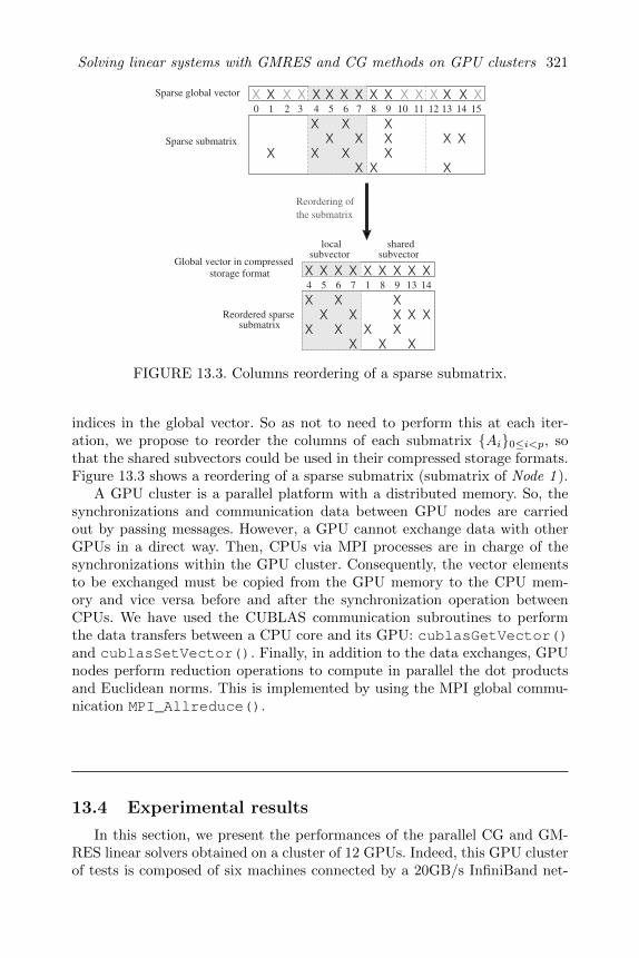
Solving linear systems with GMRES and CG methods on GPU clusters 321
X
X
X
X
X
X
X
X X
X
X
X
X
X X
0 1 2 43 8 976 105 11 14 151312
X X X X X XX X X X X X X X XX
X X X X X
4 5 6 7 1
X X X X
8 9 13 14
X
X
X
X
X X
X
X
X
X
X
X
X
X
X
Sparse global vector
Sparse submatrix
Reordering of
the submatrix
subvector subvectorlocal shared
Reordered sparsesubmatrix
storage format
Global vector in compressed
FIGURE 13.3. Columns reordering of a sparse submatrix.
indices in the global vector. So as not to need to perform this at each iter-ation, we propose to reorder the columns of each submatrix Ai0≤i<p, sothat the shared subvectors could be used in their compressed storage formats.Figure 13.3 shows a reordering of a sparse submatrix (submatrix of Node 1 ).
A GPU cluster is a parallel platform with a distributed memory. So, thesynchronizations and communication data between GPU nodes are carriedout by passing messages. However, a GPU cannot exchange data with otherGPUs in a direct way. Then, CPUs via MPI processes are in charge of thesynchronizations within the GPU cluster. Consequently, the vector elementsto be exchanged must be copied from the GPU memory to the CPU mem-ory and vice versa before and after the synchronization operation betweenCPUs. We have used the CUBLAS communication subroutines to performthe data transfers between a CPU core and its GPU: cublasGetVector()and cublasSetVector(). Finally, in addition to the data exchanges, GPUnodes perform reduction operations to compute in parallel the dot productsand Euclidean norms. This is implemented by using the MPI global commu-nication MPI_Allreduce().
13.4 Experimental results
In this section, we present the performances of the parallel CG and GM-RES linear solvers obtained on a cluster of 12 GPUs. Indeed, this GPU clusterof tests is composed of six machines connected by a 20GB/s InfiniBand net-

322 Designing Scientific Applications on GPUs
240 cores
PCIe 8GB/s
25.6GB/s
Quad−Core CPU
CORE 1
CORE 2
CORE 3
CORE 4
12GB
GPU 1
102GB/s
240 cores
GPU 2
102GB/s
4GB4GB
Device memory
Host memory
Device memory
Node 2
Node
1
Machine 1
240 cores
PCIe 8GB/s
25.6GB/s
Quad−Core CPU
CORE 1
CORE 2
CORE 3
CORE 4
12GB
GPU 1
102GB/s
240 cores
GPU 2
102GB/s
4GB4GB
Device memory
Host memory
Device memory
Node 4
Node
3
Machine 2
240 cores
PCIe 8GB/s
25.6GB/s
Quad−Core CPU
CORE 1
CORE 2
CORE 3
CORE 4
12GB
GPU 1
102GB/s
240 cores
GPU 2
102GB/s
4GB4GB
Device memory
Host memory
Device memory
Node 1
2Node
11
Machine 6
Infiniband 20GB/s
FIGURE 13.4. General scheme of the GPU cluster of tests composed of sixmachines, each with two GPUs.
work. Each machine is a Quad-Core Xeon E5530 CPU running at 2.4GHz andproviding 12GB of RAM with a memory bandwidth of 25.6GB/s. In addition,two Tesla C1060 GPUs are connected to each machine via a PCI-Express 16xGen 2.0 interface with a throughput of 8GB/s. A Tesla C1060 GPU contains240 cores running at 1.3GHz and providing a global memory of 4GB with amemory bandwidth of 102GB/s. Figure 13.4 shows the general scheme of theGPU cluster that we used in the experimental tests.
Linux cluster version 2.6.39 OS is installed on CPUs. C programminglanguage is used to code the parallel algorithms of both methods on the GPUcluster. CUDA version 4.0 [5] is used to program GPUs, using the CUBLASlibrary [4] to deal with vector operations in GPUs and, finally, MPI routinesof OpenMPI 1.3.3 are used to carry out the communications between CPUcores. Indeed, the experiments are done on a cluster of 12 computing nodes,where each node is managed by one MPI process and is composed of one CPUcore and one GPU card.
All tests are made on double-precision floating point operations. The pa-rameters of both linear solvers are initialized as follows: the residual tolerancethreshold ε = 10−12, the maximum number of iterations maxiter = 500, theright-hand side b is filled with 1.0, and the initial guess x0 is filled with 0.0.In addition, we limited the Arnoldi iterations used in the GMRES methodto 16 iterations (m = 16). For the sake of simplicity, we have chosen thepreconditioner M as the main diagonal of the sparse matrix A. Indeed, itallows us to easily compute the required inverse matrix M−1, and it providesa relatively good preconditioning for not too ill-conditioned matrices. In theGPU computing, the size of thread blocks is fixed to 512 threads. Finally, the

Solving linear systems with GMRES and CG methods on GPU clusters 323
thermal2
cage13 torso3poli_largelanguage
2cubes_sphere
crashbasis FEM_3D_thermal2
ecology2 finan512 G3_circuit shallow_water2
FIGURE 13.5. Sketches of sparse matrices chosen from the University ofFlorida collection.
Matrix Type Matrix Name # Rows # Nonzeros Bandwidth
Symmetric
2cubes sphere 101, 492 1, 647, 264 100, 464ecology2 999, 999 4, 995, 991 2, 001finan512 74, 752 596, 992 74, 725
G3 circuit 1, 585, 478 7, 660, 826 1, 219, 059shallow water2 81, 920 327, 680 58, 710
thermal2 1, 228, 045 8, 580, 313 1, 226, 629
Nonsymmetric
cage13 445, 315 7, 479, 343 318, 788crashbasis 160, 000 1, 750, 416 120, 202
FEM 3D thermal2 147, 900 3, 489.300 117, 827language 399, 130 1, 216, 334 398, 622poli large 15, 575 33, 074 15, 575
torso3 259, 156 4, 429, 042 216, 854
TABLE 13.1. Main characteristics of sparse matrices chosen from the Univer-sity of Florida collection.
performance results, presented hereafter, are obtained from the mean valueover 10 executions of the same parallel linear solver and for the same inputdata.
To get more realistic results, we have tested the CG and GMRES algo-rithms on sparse matrices of the University of Florida collection [6], that arisein a wide spectrum of real-world applications. We have chosen six symmetricsparse matrices and six nonsymmetric ones from this collection. In Figure 13.5,we show the structures of these matrices and in Table 13.1 we present theirmain characteristics which are the number of rows, the total number of nonzerovalues, and the maximal bandwidth. In the present chapter, the bandwidthof a sparse matrix is defined as the number of matrix columns separating thefirst and the last nonzero value on a matrix row.
Tables 13.2 and 13.3 show the performances of the parallel CG and GM-

324 Designing Scientific Applications on GPUs
Matrix Timecpu Timegpu τ # Iter. Prec. ∆
2cubes sphere 0.132s 0.069s 1.93 12 1.14e-09 3.47e-18ecology2 0.026s 0.017s 1.52 13 5.06e-09 8.33e-17finan512 0.053s 0.036s 1.49 12 3.52e-09 1.66e-16
G3 circuit 0.704s 0.466s 1.51 16 4.16e-10 4.44e-16shallow water2 0.017s 0.010s 1.68 5 2.24e-14 3.88e-26
thermal2 1.172s 0.622s 1.88 15 5.11e-09 3.33e-16
TABLE 13.2. Performances of the parallel CG method on a cluster of 24 CPUcores vs. on a cluster of 12 GPUs.
Matrix Timecpu Timegpu τ # Iter. Prec. ∆
2cubes sphere 0.234s 0.124s 1.88 21 2.10e-14 3.47e-18ecology2 0.076s 0.035s 2.15 21 4.30e-13 4.38e-15finan512 0.073s 0.052s 1.40 17 3.21e-12 5.00e-16
G3 circuit 1.016s 0.649s 1.56 22 1.04e-12 2.00e-15shallow water2 0.061s 0.044s 1.38 17 5.42e-22 2.71e-25
thermal2 1.666s 0.880s 1.89 21 6.58e-12 2.77e-16
cage13 0.721s 0.338s 2.13 26 3.37e-11 2.66e-15crashbasis 1.349s 0.830s 1.62 121 9.10e-12 6.90e-12
FEM 3D thermal2 0.797s 0.419s 1.90 64 3.87e-09 9.09e-13language 2.252s 1.204s 1.87 90 1.18e-10 8.00e-11poli large 0.097s 0.095s 1.02 69 4.98e-11 1.14e-12
torso3 4.242s 2.030s 2.09 175 2.69e-10 1.78e-14
TABLE 13.3. Performances of the parallel GMRES method on a cluster 24CPU cores vs. on cluster of 12 GPUs.
RES solvers, respectively, for solving linear systems associated to the sparsematrices presented in Table 13.1. They allow us to compare the performancesobtained on a cluster of 24 CPU cores and on a cluster of 12 GPUs. However,Table 13.2 shows the performances of solving only symmetric sparse linearsystems, due to the inability of the CG method to solve the nonsymmetricsystems. In both tables, the second and third columns give, respectively, theexecution times in seconds obtained on 24 CPU cores (Timecpu) and thatobtained on 12 GPUs (Timegpu). Moreover, we take into account the relativegains τ of a solver implemented on the GPU cluster compared to the samesolver implemented on the CPU cluster. The relative gains, presented in thefourth column, are computed as a ratio of the CPU execution time over theGPU execution time:
τ =TimecpuTimegpu
. (13.20)
In addition, Tables 13.2 and 13.3 give the number of iterations (iter), the pre-

Solving linear systems with GMRES and CG methods on GPU clusters 325
cision (prec) of the solution computed on the GPU cluster, and the difference∆ between the solution computed on the CPU cluster and that computed onthe GPU cluster. Both parameters prec and ∆ allow us to validate and verifythe accuracy of the solution computed on the GPU cluster. We have computedthem as follows:
∆ = max|xcpu − xgpu|, (13.21)
prec = max|M−1rgpu|, (13.22)
where ∆ is the maximum vector element, in absolute value, of the differencebetween the two solutions xcpu and xgpu computed, respectively, on CPU andGPU clusters and prec is the maximum element, in absolute value, of theresidual vector rgpu ∈ Rn of the solution xgpu. Thus, we can see that the solu-tions obtained on the GPU cluster were computed with a sufficient accuracy(about 10−10) and they are, more or less, equivalent to those computed onthe CPU cluster with a small difference ranging from 10−10 to 10−26. How-ever, we can notice from the relative gains τ that it is not efficient to usemultiple GPUs for solving small sparse linear systems. In fact, a small sparsematrix does not allow us to maximize utilization of GPU cores. In addition,the communications required to synchronize the computations over the clus-ter increase the idle times of GPUs and slow down the parallel computationsfurther.
Consequently, in order to test the performances of the parallel solvers, wedeveloped in C programming language a generator of large sparse matrices.This generator takes a matrix from the University of Florida collection [6] as aninitial matrix to build large sparse matrices exceeding ten million rows. It mustbe executed in parallel by the MPI processes of the computing nodes, so thateach process can build its sparse submatrix. In the first experimental tests, wefocused on sparse matrices having a banded structure, because they are thosearising the most in the majority of numerical problems. So to generate theglobal sparse matrix, each MPI process constructs its submatrix by performingseveral copies of an initial sparse matrix chosen from the University of Floridacollection. Then, it puts all these copies on the main diagonal of the globalmatrix (see Figure 13.6). Moreover, the empty spaces between two successivecopies in the main diagonal are filled with subcopies (left-copy and right-copyin Figure 13.6) of the same initial matrix.
We have used the parallel CG and GMRES algorithms for solving sparselinear systems of 25 million unknown values. The sparse matrices associated tothese linear systems are generated from those presented in Table 13.1. Theirmain characteristics are given in Table 13.4. Tables 13.5 and 13.6 show theperformances of the parallel CG and GMRES solvers, respectively, obtainedon a cluster of 24 CPU cores and on a cluster of 12 GPUs. Obviously, wecan notice from these tables that solving large sparse linear systems on aGPU cluster is more efficient than on a CPU cluster (see relative gains τ).We can also notice that the execution times of the CG method, whether ina CPU cluster or in a GPU cluster, are better than those of the GMRES

326 Designing Scientific Applications on GPUs
offset2
offset1
offset0
offset3
right−copy
Initial sparse matrix
left−copy
right−copy
Global sparse matrix
left−copy
Node 0
Node 1
Node 3
Node 2
FIGURE 13.6. Parallel generation of a large sparse matrix by four computingnodes.
Matrix Type Matrix Name # Nonzeros Bandwidth
Symmetric
2cubes sphere 413, 703, 602 198, 836ecology2 124, 948, 019 2, 002finan512 278, 175, 945 123, 900
G3 circuit 125, 262, 292 1, 891, 887shallow water2 100, 235, 292 62, 806
thermal2 175, 300, 284 2, 421, 285
Nonsymmetric
cage13 435, 770, 480 352, 566crashbasis 409, 291, 236 200, 203
FEM 3D thermal2 595, 266, 787 206, 029language 76, 912, 824 398, 626poli large 53, 322, 580 15, 576
torso3 433, 795, 264 328, 757
TABLE 13.4. Main characteristics of sparse banded matrices generated fromthose of the University of Florida collection.
method for solving large symmetric linear systems. In fact, the CG methodis characterized by a better convergence rate and a shorter execution time ofan iteration than those of the GMRES method. Moreover, an iteration of theparallel GMRES method requires more data exchanges between computingnodes compared to the parallel CG method.

Solving linear systems with GMRES and CG methods on GPU clusters 327
Matrix Timecpu Timegpu τ # Iter. Prec. ∆
2cubes sphere 1.625s 0.401s 4.05 14 5.73e-11 5.20e-18ecology2 0.856s 0.103s 8.27 15 3.75e-10 1.11e-16finan512 1.210s 0.354s 3.42 14 1.04e-10 2.77e-16
G3 circuit 1.346s 0.263s 5.12 17 1.10e-10 5.55e-16shallow water2 0.397s 0.055s 7.23 7 3.43e-15 5.17e-26
thermal2 1.411s 0.244s 5.78 16 1.67e-09 3.88e-16
TABLE 13.5. Performances of the parallel CG method for solving linear sys-tems associated to sparse banded matrices on a cluster of 24 CPU cores vs.on a cluster of 12 GPUs.
Matrix Timecpu Timegpu τ # Iter. Prec. ∆
2cubes sphere 3.597s 0.514s 6.99 21 2.11e-14 8.67e-18ecology2 2.549s 0.288s 8.83 21 4.88e-13 2.08e-14finan512 2.660s 0.377s 7.05 17 3.22e-12 8.82e-14
G3 circuit 3.139s 0.480s 6.53 22 1.04e-12 5.00e-15shallow water2 2.195s 0.253s 8.68 17 5.54e-21 7.92e-24
thermal2 3.206s 0.463s 6.93 21 8.89e-12 3.33e-16
cage13 5.560s 0.663s 8.39 26 3.29e-11 1.59e-14crashbasis 25.802s 3.511s 7.35 135 6.81e-11 4.61e-15
FEM 3D thermal2 13.281s 1.572s 8.45 64 3.88e-09 1.82e-12language 12.553s 1.760s 7.13 89 2.11e-10 1.60e-10poli large 8.515s 1.053s 8.09 69 5.05e-11 6.59e-12
torso3 31.463s 3.681s 8.55 175 2.69e-10 2.66e-14
TABLE 13.6. Performances of the parallel GMRES method for solving linearsystems associated to sparse banded matrices on a cluster of 24 CPU coresvs. on a cluster of 12 GPUs.
13.5 Conclusion
In this chapter, we have aimed at harnessing the computing power of acluster of GPUs for solving large sparse linear systems. For this, we have usedtwo Krylov subspace iterative methods: the CG and GMRES methods. Thefirst method is well known for its efficiency to solve symmetric linear systemsand the second one is used, particularly, to solve nonsymmetric linear systems.
We have presented the parallel implementation of both iterative methodson a GPU cluster. Particularly, the operations dealing with the vectors and/or

328 Designing Scientific Applications on GPUs
matrices, of these methods, are parallelized between the different GPU com-puting nodes of the cluster. Indeed, the data-parallel vector operations areaccelerated by GPUs, and the communications required to synchronize theparallel computations are carried out by CPU cores. For this, we have usedheterogeneous CUDA/MPI programming to implement the parallel iterativealgorithms.
In the experimental tests, we have shown that using a GPU cluster isefficient for solving linear systems associated to very large sparse matrices.The experimental results, discussed in the present chapter, show that a clusterof 12 GPUs is about 7 times faster than a cluster of 24 CPU cores for solvinglarge sparse linear systems of 25 million unknown values. This is due to theGPUs ability to compute the data-parallel operations faster than the CPUs.
In our future works, we plan to test the parallel algorithms of CG and GM-RES methods, adapted to GPUs, for solving large linear systems associatedto sparse matrices of different structures. For example, the matrices havinglarge bandwidths can lead to many data dependencies between the comput-ing nodes and, thus, degrade the performances of both algorithms. So in thiscase, it would be interesting to study the different data partitioning tech-niques, in order to minimize the dependencies between the computing nodesand thus to reduce the total communication volume. This may improve theperformances of both algorithms implemented on a GPU cluster. Moreover, inthe recent GPU hardware and software architectures, the GPU-Direct systemwith CUDA version 5.0 is used so that two GPUs located on the same node oron distant nodes can communicate between each other directly without CPUs.This allows us to improve the data transfers between GPUs.
Bibliography
[1] CUSP Library. http://code.google.com/p/cusp-library/.
[2] W.E. Arnoldi. The principle of minimized iteration in the solution of thematrix eigenvalue problem. Quarterly of Applied Mathematics, 9(17):17–29, 1951.
[3] N. Bell and M. Garland. Efficient sparse matrix-vector multiplication onCUDA. NVIDIA Technical Report NVR-2008-004, NVIDIA Corporation,December 2008.
[4] NVIDIA Corporation. CUDA Toolkit 4.2 CUBLAS Library. 2012. http://developer.download.nvidia.com/compute/DevZone/docs/html/CUDALibraries/doc/CUBLAS_Library.pdf.
[5] NVIDIA Corporation. NVIDIA CUDA C Programming Guide. 2012.Version 4.2.

Solving linear systems with GMRES and CG methods on GPU clusters 329
[6] T. Davis and Y. Hu. The University of Florida Sparse Matrix Col-lection. 1997. http://www.cise.ufl.edu/research/sparse/matrices/list_by_id.html.
[7] M.R. Hestenes and E. Stiefel. Methods of conjugate gradients for solvinglinear systems. Journal of Research of the National Bureau of Standards,49(6):409–436, 1952.
[8] C.C. Paige and M.A. Saunders. Solution of sparse indefinite systems oflinear equations. SIAM Journal on Numerical Analysis, 12(4):617–629,1975.
[9] Y. Saad. Iterative Methods for Sparse Linear Systems. Society for Indus-trial and Applied Mathematics, second edition, 2003.
[10] Y. Saad and M.H. Schultz. GMRES: a generalized minimal residualalgorithm for solving nonsymmetric linear systems. SIAM Journal onScientific and Statistical Computing, 7(3):856–869, 1986.

This page intentionally left blankThis page intentionally left blank
Chapter 14
Solving sparse nonlinear systems ofobstacle problems on GPU clusters
Lilia Ziane Khodja, Raphael Couturier, and Jacques Bahi
Femto-ST Institute, University of Franche-Comte, France
Ming Chau
Advanced Solutions Accelerator, Castelnau Le Lez, France
Pierre Spiteri
ENSEEIHT-IRIT, Toulouse, France
14.1 Introduction . . . . . . . . . . . . . . . . . . . . . . . . . . . . . . . . . . . . . . . . . . . . . . . . . . . . . . 33114.2 Obstacle problems . . . . . . . . . . . . . . . . . . . . . . . . . . . . . . . . . . . . . . . . . . . . . . . . 332
14.2.1 Mathematical model . . . . . . . . . . . . . . . . . . . . . . . . . . . . . . . . . . . . . 33214.2.2 Discretization . . . . . . . . . . . . . . . . . . . . . . . . . . . . . . . . . . . . . . . . . . . . 333
14.3 Parallel iterative method . . . . . . . . . . . . . . . . . . . . . . . . . . . . . . . . . . . . . . . . . 33414.4 Parallel implementation on a GPU cluster . . . . . . . . . . . . . . . . . . . . . . 33714.5 Experimental tests on a GPU cluster . . . . . . . . . . . . . . . . . . . . . . . . . . . . 34514.6 Red-black ordering technique . . . . . . . . . . . . . . . . . . . . . . . . . . . . . . . . . . . . 34814.7 Conclusion . . . . . . . . . . . . . . . . . . . . . . . . . . . . . . . . . . . . . . . . . . . . . . . . . . . . . . . . 352
Bibliography . . . . . . . . . . . . . . . . . . . . . . . . . . . . . . . . . . . . . . . . . . . . . . . . . . . . . . 353
14.1 Introduction
The obstacle problem is one kind of free boundary problem. It allowsus to model, for example, an elastic membrane covering a solid obstacle. Inthis case, the objective is to find an equilibrium position of this membraneconstrained to be above the obstacle and which tends to minimize its surfaceand/or its energy. The study of such problems occurs in many applications, forexample, fluid mechanics, biomathematics (tumor growth process), or financialmathematics (American or European option pricing).
In this chapter, we focus on solutions of large obstacle problems defined ina three-dimensional domain. Particularly, the present study consists of solvinglarge nonlinear systems derived from the spatial discretization of these prob-lems. Owing to the great size of such systems, in order to reduce computation
331

332 Designing Scientific Applications on GPUs
times, we proceed by solving them by parallel synchronous or asynchronousiterative algorithms. Moreover, we aim at harnessing the computing power ofGPUs to accelerate computations of these parallel algorithms. For this, weuse an iterative method involving a projection on a convex set, which is theprojected Richardson method. We chose this method among other iterativemethods because it is easy to implement on parallel computers and easy toadapt to GPU architectures.
In Section 14.2, we present the mathematical model of obstacle problemsthen, in Section 14.3, we describe the general principle of the parallel pro-jected Richardson method. Next, in Section 14.4, we give the main key pointsof the parallel implementation of both synchronous and asynchronous algo-rithms of the projected Richardson method on a GPU cluster. In Section 14.5,we present the performances of both parallel algorithms obtained from sim-ulations carried out on GPU clusters. Finally, in Section 14.6, we use theread-black ordering technique to improve the convergence and, thus, the ex-ecution times of the parallel projected Richardson algorithms on the GPUcluster.
14.2 Obstacle problems
In this section, we present the mathematical model of obstacle problemsdefined in a three-dimensional domain. This model is based on that presentedin [5].
14.2.1 Mathematical model
An obstacle problem, arising for example in mechanics or financial deriva-tives, consists of solving a time-dependent nonlinear equation:
∂u∂t + bt.∇u− η.∆u+ c.u− f ≥ 0, u ≥ φ, a.e.w. in [0, T ]× Ω, η > 0,(∂u∂t + bt.∇u− η.∆u+ c.u− f)(u− φ) = 0, a.e.w. in [0, T ]× Ω,u(0, x, y, z) = u0(x, y, z),B.C. on u(t, x, y, z) defined on ∂Ω,
(14.1)where u0 is the initial condition; c ≥ 0, b, and η are physical parameters;T is the final time; u = u(t, x, y, z) is an element of the solution vector Uto compute; f is the right-hand side that could represent, for example, theexternal forces; B.C. describes the boundary conditions on the boundary ∂Ωof the domain Ω; φ models a constraint imposed to u; ∆ is the Laplacianoperator; ∇ is the gradient operator; a.e.w. means almost everywhere, and “.”defines the products between two scalars, a scalar and a vector, or a matrixand a vector. In practice the boundary condition, generally considered, is the

Solving sparse nonlinear systems of obstacle problems on GPU clusters 333
Dirichlet condition (where u is fixed on ∂Ω) or the Neumann condition (wherethe normal derivative of u is fixed on ∂Ω).
The time-dependent equation (14.1) is numerically solved by consideringan implicit or a semi-implicit time marching, where at each time step k astationary nonlinear problem is solved: bt.∇u− η.∆u+ (c+ δ).u− g ≥ 0, u ≥ φ, a.e.w. in [0, T ]× Ω, η > 0,
(bt.∇u− η.∆u+ (c+ δ).u− g)(u− φ) = 0, a.e.w. in [0, T ]× Ω,B.C. on u(t, x, y, z) defined on ∂Ω,
(14.2)where δ = 1
k is the inverse of the time step k, g = f + δuprev and uprev is thesolution computed at the previous time step.
14.2.2 Discretization
First, we note that the spatial discretization of the previous stationaryproblem (14.2) does not provide a symmetric matrix, because the convection-diffusion operator is not self-adjoint. Moreover, the fact that the operator isself-adjoint or not plays an important role in the choice of the appropriatealgorithm for solving nonlinear systems derived from the discretization of theobstacle problem. Nevertheless, since the convection coefficients arising in theoperator (14.2) are constant, we can formulate the same problem by self-adjoint operator by performing a classical change of variables. Then, we canreplace the stationary convection-diffusion problem:
bt.∇v − η.∆v + (c+ δ).v = g, a.e.w. in [0, T ]× Ω, c ≥ 0, δ ≥ 0, (14.3)
by the following stationary diffusion operator:
−η.∆u+ (‖b‖224η
+ c+ δ).u = e−ag = f, (14.4)
where b = b1, b2, b3, ‖b‖2 denotes the Euclidean norm of b, and v = e−a.u
represents the general change of variables such that a = bt(x,y,z)2η . Conse-
quently, the numerical resolution of the diffusion problem (the self-adjointoperator (14.4)) is done by optimization algorithms, in contrast to that of theconvection-diffusion problem (nonself-adjoint operator (14.3)) which is doneby relaxation algorithms. In the case of our studied algorithm, the conver-gence is ensured by M-matrix property; then, the performance is linked to themagnitude of the spectral radius of the iteration matrix, which is independentof the condition number.
Next, the three-dimensional domain Ω ⊂ R3 is set to Ω = [0, 1]3 and dis-cretized with a uniform Cartesian mesh constituted by M = m3 discretizationpoints, where m is related to the spatial discretization step by h = 1
m+1 . Thisis carried out by using a classical order 2 finite difference approximation ofthe Laplacian. So, the complete discretization of both stationary boundary

334 Designing Scientific Applications on GPUs
value problems (14.3) and (14.4) leads to the solution of a large discrete com-plementary problem of the following form, when both Dirichlet or Neumannboundary conditions are used:
Find U∗ ∈ RM such that(A+ δI)U∗ −G ≥ 0, U∗ ≥ Φ,((A+ δI)U∗ −G)T (U∗ − Φ) = 0,
(14.5)
where A is a matrix obtained after the spatial discretization by a finite differ-ence method, G is derived from the Euler first order implicit time marchingscheme and from the discretized right-hand side of the obstacle problem, δis the inverse of the time step k, and I is the identity matrix. The matrix Ais symmetric when the self-adjoint operator is considered and nonsymmetricotherwise.
According to the chosen discretization scheme of the Laplacian, A is an M-matrix (irreducibly diagonal dominant, see [15]) and, consequently, the matrix(A+ δI) is also an M-matrix. This property is important to the convergenceof iterative methods.
14.3 Parallel iterative method
Owing to the large size of the previous discrete complementary prob-lem (14.5), we will solve it by parallel synchronous or asynchronous iterativealgorithms (see [1–3]). In this chapter, we aim at harnessing the computingpower of GPU clusters for solving these large nonlinear systems. Then, wechoose to use the projected Richardson iterative method for solving the dif-fusion problem (14.4). Indeed, this method is based on the iterations of theJacobi method, which are easy to parallelize on parallel computers and easyto adapt to GPU architectures. Then, according to the boundary value prob-lem formulation with a self-adjoint operator (14.4), we can consider here theequivalent optimization problem and the fixed point mapping associated toits solution.
Assume that E = RM is a Hilbert space, in which 〈. , .〉 is the scalar productand ‖.‖ its associated norm. So, the general fixed point problem to be solvedis defined as follows:
Find U∗ ∈ E such thatU∗ = F (U∗),
(14.6)
where U 7→ F (U) is an application from E to E.Let K be a closed convex set defined by
K = U |U ≥ Φ everywhere in E, (14.7)

Solving sparse nonlinear systems of obstacle problems on GPU clusters 335
where Φ is the discrete obstacle function. In fact, the obstacle problem (14.5)is formulated as the following constrained optimization problem:
Find U∗ ∈ K such that∀V ∈ K,J(U∗) ≤ J(V ),
(14.8)
where the cost function is given by
J(U) =1
2〈A.U , U〉 − 〈G ,U〉, (14.9)
in which 〈. , .〉 denotes the scalar product in E, A = A + δI is a symmetricpositive definite, and A is the discretization matrix associated with the self-adjoint operator (14.4) after change of variables.
For any U ∈ E; let PK(U) be the projection of U on K. For any γ ∈ R,γ > 0, the fixed point mapping Fγ of the projected Richardson method isdefined as follows:
U∗ = Fγ(U∗) = PK(U∗ − γ(A.U∗ −G)). (14.10)
In order to reduce the computation time, the large optimization problemis solved in a numerical way by using a parallel asynchronous algorithmof the projected Richardson method on the convex set K. Particularly, wewill consider an asynchronous parallel adaptation of the projected Richardsonmethod [12].
Let α ∈ N be a positive integer. We consider that the space E =
α∏i=1
Ei is
a product of α subspaces Ei where i ∈ 1, . . . , α. Note that Ei = Rmi , whereα∑i=1
mi = M , is also a Hilbert space in which 〈. , .〉i denotes the scalar product
and |.|i the associated norm, for all i ∈ 1, . . . , α. Then, for all u, v ∈ E,
〈u , v〉 =
α∑i=1
〈ui , vi〉i is the scalar product on E.
Let U ∈ E, we consider the following decomposition of U and the corre-sponding decomposition of Fγ into α blocks:
U = (U1, . . . , Uα),Fγ(U) = (F1,γ(U), . . . , Fα,γ(U)).
(14.11)
Assume that the convex set K =
α∏i=1
Ki, such that ∀i ∈ 1, . . . , α,Ki ⊂ Ei,
and Ki is a closed convex set. Let also G = (G1, . . . , Gα) ∈ E; for any U ∈ E,PK(U) = (PK1
(U1), . . . , PKα(Uα)) is the projection of U on K where ∀i ∈1, . . . , α, PKi is the projector from Ei onto Ki. So, the fixed point mappingof the projected Richardson method (14.10) can be written in the followingway:
∀U ∈ E, ∀i ∈ 1, . . . , α, Fi,γ(U) = PKi(Ui − γ(Ai.U −Gi)). (14.12)

336 Designing Scientific Applications on GPUs
Note that Ai.U =
α∑j=1
Ai,j .Uj , where Ai,j denote block matrices of A.
The parallel asynchronous iterations of the projected Richardson methodfor solving the obstacle problem (14.8) are defined as follows: let U0 ∈ E,U0 =(U0
1 , . . . , U0α) be the initial solution, then for all p ∈ N, the iterate Up+1 =
(Up+11 , . . . , Up+1
α ) is recursively defined by
Up+1i =
Fi,γ(U
ρ1(p)1 , . . . , U
ρα(p)α ) if i ∈ s(p),
Upi otherwise,(14.13)
where ∀p ∈ N, s(p) ⊂ 1, . . . , α and s(p) 6= ∅,∀i ∈ 1, . . . , α, p | i ∈ s(p) is enumerable,
(14.14)
and ∀j ∈ 1, . . . , α,∀p ∈ N, ρj(p) ∈ N, 0 ≤ ρj(p) ≤ p and ρj(p) = p if j ∈ s(p),limp→∞
ρj(p) = +∞. (14.15)
The previous asynchronous scheme of the projected Richardson methodmodels computations that are carried out in parallel without order or syn-chronization (according to the behavior of the parallel iterative method) anddescribes a subdomain method without overlapping. It is a general modelthat takes into account all possible situations of parallel computations andnonblocking message passing. So, the synchronous iterative scheme is definedby
∀j ∈ 1, . . . , α, ∀p ∈ N, ρj(p) = p. (14.16)
The values of s(p) and ρj(p) are defined dynamically and not explicitly bythe parallel asynchronous or synchronous execution of the algorithm. Particu-larly, They allow us to consider distributed computations whereby processorscompute at their own pace according to their intrinsic characteristics andcomputational load. The parallelism between the processors is well describedby the set s(p) which contains at each step p the index of the componentsrelaxed by each processor on a parallel way while the use of delayed compo-nents in (14.13) permits one to model nondeterministic behavior and does notimply inefficiency of the considered distributed scheme of computation. Notethat, according to [11], theoretically, each component of the vector must berelaxed an infinite number of times. The choice of the relaxed components tobe used in the computational process may be guided by any criterion, and inparticular, a natural criterion is to pickup the most recently available values ofthe components computed by the processors. Furthermore, the asynchronousiterations are implemented by means of nonblocking MPI communication sub-routines (asynchronous communications).
The important property ensuring the convergence of the parallel projectedRichardson method, both synchronous and asynchronous algorithms, is the

Solving sparse nonlinear systems of obstacle problems on GPU clusters 337
fact that A is an M-matrix. Moreover, the convergence proceeds from a resultof [12]. Indeed, there exists a value γ0 > 0, such that ∀γ ∈]0, γ0[, the paralleliterations (14.13), (14.14), and (14.15), associated to the fixed point mappingFγ (14.12), converge to the unique solution U∗ of the discretized problem.
14.4 Parallel implementation on a GPU cluster
In this section, we give the main key points of the parallel implementa-tion of the projected Richardson method, both synchronous and asynchronousversions, on a GPU cluster, for solving the nonlinear systems derived fromthe discretization of large obstacle problems. More precisely, each nonlinearsystem is solved iteratively using the whole cluster. We use a heterogeneousCUDA and MPI programming. Indeed, the communication of data, at eachiteration between the GPU computing nodes, can be either synchronous orasynchronous using the MPI communication subroutines, whereas inside eachGPU node, a CUDA parallelization is performed.
Let S denote the number of computing nodes on the GPU cluster, wherea computing node is composed of CPU core holding one MPI process anda GPU card. So, before starting computations, the obstacle problem of size(NX × NY × NZ) is split into S parallelepipedic subproblems, each for anode (MPI process, GPU), as is shown in Figure 14.1. Indeed, the NY andNZ dimensions (according to the y and z axises) of the three-dimensionalproblem are split, respectively, into Sy and Sz parts, such that S = Sy× Sz.In this case, each computing node has at most four neighboring nodes. Thiskind of data partitioning reduces the data exchanges at subdomain boundariescompared to a naive z-axis-wise partitioning.
All the computing nodes of the GPU cluster execute in parallel the Algo-rithm 17 on a three-dimensional subproblems of size (NX × ny × nz). Thisalgorithm gives the main key points for solving an obstacle problem definedin a three-dimensional domain, where A is the discretization matrix, G is theright-hand side, and U is the solution vector. After the initialization step, allthe data generated from the partitioning operation are copied from the CPUmemories to the GPU global memories to be processed on the GPUs. Next,the algorithm uses NbSteps time steps to solve the global obstacle problem. Infact, it uses a parallel algorithm adapted to GPUs from the projected Richard-son iterative method for solving the nonlinear systems of the obstacle problem.This function is defined by Solve() in Algorithm 17. At every time step, theinitial guess U0 for the iterative algorithm is set to the solution found at theprevious time step. Moreover, the right-hand side G is computed as follows:
G =1
k.Uprev + F

338 Designing Scientific Applications on GPUs
node0
node1
node2
node3
node4
node5
node6
node7
node8
node10
Bordering points
NX
nz
ny
NY
NZ
NX x
z
node11
node9
y
FIGURE 14.1. Data partitioning of a problem to be solved among S = 3× 4computing nodes.
Algorithm 17: parallel solving of the obstacle problem on a GPU cluster
1 Initialization of the parameters of the subproblem;2 Allocate and fill the data in the global memory GPU;3 for i = 1 to NbSteps do4 G = 1
k .U0 + F ;
5 Solve(A, U0, G, U , ε, MaxRelax);6 U0 = U ;
7 end8 Copy the solution U back from GPU memory;
where k is the time step, Uprev is the solution computed in the previous timestep, and each element f(x, y, z) of the vector F is computed as follows:
f(x, y, z) = cos(2πx) · cos(4πy) · cos(6πz). (14.17)
Finally, the solution U of the obstacle problem is copied back from theGPU global memories to the CPU memories. We use the communicationsubroutines of the CUBLAS (CUDA Basic Linear Algebra Subroutines) li-brary [6] for the memory allocations in the GPU (cublasAlloc()) and thedata transfers between the CPU and its GPU: cublasSetVector() andcublasGetVector().
As are many other iterative methods, the algorithm of the projectedRichardson method is based on algebraic functions operating on vectorsand/or matrices, which are more efficient on parallel computers when they

Solving sparse nonlinear systems of obstacle problems on GPU clusters 339
Algorithm 18: parallel iterative solving of the nonlinear systems on aGPU cluster (Solve() function)
1 p = 0;2 conv = false;3 U = U0;4 repeat5 Determine Bordering Vector Elements(U);6 Compute New Vector Elements(A, G, U);7 tmp = U0 − U ;8 error = ‖tmp‖2;9 U0 = U ;
10 p = p+ 1;11 conv = Convergence(error, p, ε, MaxRelax);
12 until (conv = true);
work on large vectors. Its parallel implementation on the GPU cluster is car-ried out so that the GPUs execute the vector operations as kernels and theCPUs execute the serial codes, supervise the kernel executions and the dataexchanges with the neighboring nodes, and supply the GPUs with data. Algo-rithm 18 shows the main key points of the parallel iterative algorithm (functionSolve() in Algorithm 17). All the vector operations inside the main loop (re-peat ... until) are executed by the GPU. We use the following functions ofthe CUBLAS library:
• cublasDaxpy() to compute the difference between the solution vec-tors Up and Up+1 computed in two successive relaxations p and p + 1(line 7 in Algorithm 18),
• cublasDnrm2() to perform the Euclidean norm (line 8), and
• cublasDcpy() for the data copy of a vector to another one in the GPUmemory (lines 3 and 9).
The dimensions of the grid and blocks of threads that execute a givenkernel depend on the resources of the GPU multiprocessor and the resourcerequirements of the kernel. So, if block defines the size of a thread block,which must not exceed the maximum size of a thread block, then the numberof thread blocks in the grid, denoted by grid, can be computed according tothe size of the local subproblem as follows:
grid =(NX × ny × nz) + block − 1
block.
However, when solving very large problems, the size of the thread grid canexceed the maximum number of thread blocks that can be executed on theGPUs (upto 65.535 thread blocks), and thus, the kernel will fail to launch.

340 Designing Scientific Applications on GPUs
Grid of thread blocks
Thread blocknode11
Slice (3
)
Slice (2
)
Slice (1
)
Slice (0
)nz
NX
ny
nz
Slice (
−1)
FIGURE 14.2. Decomposition of a subproblem in a GPU into nz slices.
Therefore, for each kernel, we decompose the three-dimensional subprobleminto nz two-dimensional slices of size (NX × ny), as is shown in Figure 14.2.All slices of the same kernel are executed using a for loop by NX×ny parallelthreads organized in a two-dimensional grid of two-dimensional thread blocks,as is shown in Listing 14.1. Each thread is in charge of nz discretization points(one from each slice), accessed in the GPU memory with a constant stride(NX × ny).
Listing 14.1. skeleton codes of a GPU kernel and a CPU function
/∗ GPU kernel ∗/g l o b a l void ke rne l ( . . . , int n , int nx , int ny , int s l i c e s , int
s t r i d e , . . . )
int tx = blockIdx . x ∗ blockDim . x + threadIdx . x ; //x−coordinate5 int ty = blockIdx . y ∗ blockDim . y + threadIdx . y ; //y−coordinate
int t i d = tx + ty ∗ nx ; //thread IDfor ( int i =0; i<s l i c e s ; i++)
i f ( ( tx<nx ) && ( ty<ny ) && ( t id<n) ). . .
10 t i d += s t r i d e ;
15 /∗ CPU function ∗/void Function ( . . . )
int n = NX ∗ ny ∗ nz ; //size of the subproblemint s l i c e s = nz ;
20 int s t r i d e = NX ∗ ny ;int bx = 64 , by = 4 ;int gx = (NX + bx − 1) / bx ;int gy = ( ny + by − 1) / by ;dim3 block (bx , by ) ; //dimensions of a thread block
25 dim3 gr id ( gx , gy ) ; //dimensions of the grid. . .kerne l<<<gr id , block >>>(... , n , NX, ny , s l i c e s , s t r i d e , . . . ) ;. . .

Solving sparse nonlinear systems of obstacle problems on GPU clusters 341
The function Determine Bordering V ector Elements() (line 5 in Algo-rithm 18) determines the values of the vector elements shared at the bound-aries with neighboring computing nodes. Its main operations are as follows:
1. define the values associated to the bordering points needed by the neigh-bors,
2. copy the values associated to the bordering points from the GPU to theCPU,
3. exchange the values associated to the bordering points between theneighboring CPUs, and
4. copy the received values associated to the bordering points from theCPU to the GPU.
The first operation of this function is implemented as kernels to be performedby the GPU:
• a kernel executed by NX × nz threads to define the values associatedto the bordering vector elements along the y-axis, and
• a kernel executed by NX × ny threads to define the values associatedto the bordering vector elements along the z-axis.
As mentioned previously, we develop the synchronous and asynchronous al-gorithms of the projected Richardson method. Obviously, in this scope, thesynchronous or asynchronous communications refer to the communicationsbetween the CPU cores (MPI processes) on the GPU cluster, in order toexchange the vector elements associated to subdomain boundaries. For thememory copies between a CPU core and its GPU, we use the synchronouscommunication routines of the CUBLAS library: cublasSetVector() andcublasGetVector() in the synchronous algorithm and the asynchronousones: cublasSetVectorAsync() and cublasGetVectorAsync() in theasynchronous algorithm. Moreover, we use the communication routines ofthe MPI library to carry out the data exchanges between the neighboringnodes. We use the following communication routines: MPI_Isend() andMPI_Irecv() to perform nonblocking sends and receives, respectively. Forthe synchronous algorithm, we use the MPI routine MPI_Waitall() whichputs the MPI process of a computing node in blocking status until all dataexchanges with neighboring nodes (sends and receives) are completed. In con-trast, for the asynchronous algorithms, we use the MPI routine MPI_Test()which tests the completion of a data exchange (send or receives) withoutputting the MPI process in blocking status.
The function Compute New V ector Elements() (line 6 in Algorithm 18)computes, at each iteration, the new elements of the iterate vector U . Itsgeneral code is presented in Listing 14.1 (CPU function). The iterations of

342 Designing Scientific Applications on GPUs
West
South
Rear
North
Front
East
Center
y
x
z
FIGURE 14.3. Matrix constant coefficients in a three-dimensional domain.
the projected Richardson method, based on those of the Jacobi method, aredefined as follows:
up+1(x, y, z) = 1Center (g(x, y, z)− (Center · up(x, y, z)+West · up(x− h, y, z) + East · up(x+ h, y, z)+South · up(x, y − h, z) +North · up(x, y + h, z)+Rear · up(x, y, z − h) + Front · up(x, y, z + h))),
(14.18)
where up(x, y, z) is an element of the iterate vector U computed at the it-eration p and g(x, y, z) is a vector element of the right-hand side G. Thescalars Center, West, East, South, North, Rear, and Front define constantcoefficients of the block matrix A. Figure 14.3 shows the positions of thesecoefficients in a three-dimensional domain.
The kernel implementations of the projected Richardson method on GPUsuses a perfect fine-grain multithreading parallelism. Since the projectedRichardson algorithm is implemented as a fixed point method, each kernelis executed by a large number of GPU threads such that each thread is incharge of the computation of one element of the iterate vector U . Moreover,this method uses the vector elements updates of the Jacobi method, whichmeans that each thread i computes the new value of its element up+1
i inde-
pendently of the new values up+1j , where j 6= i, of those computed in parallel
by other threads at the same iteration p+ 1. Listing 14.2 shows the GPU im-plementations of the main kernels of the projected Richardson method, whichare: the matrix-vector multiplication (MV_Multiplication()) and the vec-tor elements updates (Vector_Updates()). The codes of these kernels arebased on that presented in Listing 14.1.

Solving sparse nonlinear systems of obstacle problems on GPU clusters 343
Listing 14.2. GPU kernels of the projected Richardson method
/∗ Kernel of the matrix−vector multiplication ∗/g l o b a l void MV Mult ipl icat ion ( . . . , double∗ U, double∗ Y)
. . .
5 //Matrix coe f f i c ients f i l l e d in registers
for ( int tz =0; tz<s l i c e s ; tz++)i f ( ( tx<NX) && ( ty<ny ) && ( t id<n) )
double sum = Center ∗ f e t ch doub l e (U, t i d ) ;10 i f ( tx != 0) sum += West ∗ f e t ch doub l e (U, t id −1) ;
i f ( tx != (NX−1) ) sum += East ∗ f e t ch doub l e (U, t i d +1) ;i f ( ty != 0) sum += South ∗ f e t ch doub l e (U, t id−NX) ;i f ( ty != (ny−1) ) sum += North ∗ f e t ch doub l e (U, t i d+NX) ;i f ( tz != 0) sum += Rear ∗ f e t ch doub l e (U, t id−NX∗ny ) ;
15 i f ( tz != ( nz−1) ) sum += Front ∗ f e t ch doub l e (U, t i d+NX∗ny ) ;Y[ t i d ] = sum ;
t i d += s t r i d e ;
20
/∗ Kernel of the vector elements updates ∗/g l o b a l void Vector Updates ( . . . , double∗ G, double∗ Y, double∗ U)
25 . . .
//Matrix coef f i c ient f i l l e d in a register : Center
for ( int tz =0; tz<s l i c e s ; tz++)i f ( ( tx<NX) && ( ty<ny ) && ( t id<n) )
30 double var = (G[ t i d ]−Y[ t i d ] ) / Center + f e t ch doub l e (U, t i d ) ;i f ( var < 0 . 0 ) var = 0 . 0 ; //projectionU[ t i d ] = var ;
t i d += s t r i d e ;
35
/∗ Function to be executed by the CPU ∗/void Computation New Vector Elements (double∗A, double∗ G, double∗ U)
40 double ∗Y;//Allocate a GPU memory space for the vector Y//Configure the kernel execution : grid and block//Elements of vector U f i l l e d in the texture memory
45
MV Multipl ication<<<gr id , block >>>(... , U, Y) ;Vector Updates<<<gr id , block >>>(... , G, Y, U) ;
Each kernel is executed by NX × ny GPU threads so that nz slices of(NX × ny) vector elements are computed in a for loop. In this case, eachthread is in charge of one vector element from each slice (in total nz vec-tor elements along the z-axis). We can notice from the formula (14.18) thatthe computation of a vector element up+1(x, y, z), by a thread at iterationp + 1, requires seven vector elements computed at the previous iteration p:two vector elements in each dimension plus the vector element at the inter-section of the three axes x, y, and z (see Figure 14.4). So, to reduce thememory accesses to the high-latency global memory, the vector elements ofthe current slice can be stored in the low-latency shared memories of threadblocks, as is described in [10]. Nevertheless, the fact that the computation

344 Designing Scientific Applications on GPUs
z
x
y
A thread is in charge of one vector component
Old value
Rear
North
South
Front
West
East
FIGURE 14.4. Computation of a vector element with the projected Richard-son method.
of a vector element requires only two elements in each dimension does notallow us to maximize the data reuse from the shared memories. The compu-tation of a slice involves in total (bx + 2) × (by + 2) accesses to the globalmemory per thread block, to fill the required vector elements in the sharedmemory where bx and by are the dimensions of a thread block. Then, in or-der to optimize the memory accesses on GPUs, the elements of the iteratevector U are filled in the cache texture memory (see [9]). In new GPU hard-ware and software as Fermi or Kepler, the global memory accesses are alwayscached in L1 and L2 caches. For example, for a given kernel, we can favorthe use of the L1 cache to that of the shared memory by using the func-tion cudaFuncSetCacheConfig(Kernel,cudaFuncCachePreferL1).So, the initial access to the global memory loads the vector elements requiredby the threads of a block into the cache memory (texture or L1/L2 caches).Then, all the following memory accesses read from this cache memory. In List-ing 14.2, the function fetch_double(v,i) is used to read from the texturememory the ith element of the double-precision vector v (see Listing 14.3).Moreover, the seven constant coefficients of matrix A can be stored in theconstant memory but, since they are reused nz times by each thread, it ismore efficient to fill them on the low-latency registers of each thread.

Solving sparse nonlinear systems of obstacle problems on GPU clusters 345
Listing 14.3. memory access to the cache texture memory
texture<int2 ,1> v ;
stat ic i n l i n ed e v i c e double f e t ch doub l e ( texture<int2 ,1> v , int i )
5 i n t2 w = tex1Dfetch (v , i ) ;return h i l o i n t 2 d o u b l e (w. y , w. x ) ;
The function Convergence() (line 11 in Algorithm 18) allows us to detectthe convergence of the parallel iterative algorithm and is based on the tolerancethreshold ε and the maximum number of relaxations MaxRelax. We take intoaccount the number of relaxations since that of iterations cannot be computedin the asynchronous case. Indeed, a relaxation is the update (14.13) of a localiterate vector Ui according to Fi. Then, counting the number of relaxations ispossible in both synchronous and asynchronous cases. On the other hand, aniteration is the update of at least all vector components with Fi.
In the synchronous algorithm, the global convergence is detected when themaximal value of the absolute error, error, is sufficiently small and/or themaximum number of relaxations, MaxRelax, is reached, as follows:
error = ‖Up − Up+1‖2;AllReduce(error, maxerror, MAX);if((maxerror < ε) or (p ≥MaxRelax))conv ← true;
where the function AllReduce() uses the MPI global reduction subroutineMPI_Allreduce() to compute the maximal value, maxerror, among thelocal absolute errors, error, of all computing nodes, and p (in Algorithm 18)is used as a counter of the local relaxations carried out by a computing node.In the asynchronous algorithms, the global convergence is detected when allcomputing nodes locally converge. For this, we use a token ring architecturearound which a boolean token travels, in one direction, from a computingnode to another. Starting from node 0, the boolean token is set to true bynode i if the local convergence is reached or to false otherwise, and then, itis sent to node i+ 1. Finally, the global convergence is detected when node 0receives from its neighbor node S − 1, in the ring architecture, a token set totrue. In this case, node 0 sends a stop message (end of parallel solving) to allcomputing nodes in the cluster.
14.5 Experimental tests on a GPU cluster
The GPU cluster of tests that we used in this chapter is an 20GB/s Infini-band network of six machines. Each machine is a Quad-Core Xeon E5530 CPU
346 Designing Scientific Applications on GPUs
running at 2.4GHz. It provides a RAM memory of 12GB with a memory band-width of 25.6GB/s and it is equipped with two NVIDIA Tesla C1060 GPUs.A Tesla GPU contains in total 240 cores running at 1.3GHz. It provides 4GBof global memory with a memory bandwidth of 102GB/s, accessible by all itscores and also by the CPU through the PCI-Express 16x Gen 2.0 interfacewith a throughput of 8GB/s. Hence, the memory copy operations between theGPU and the CPU are about 12 times slower than those of the Tesla GPUmemory. We have performed our simulations on a cluster of 24 CPU cores andon a cluster of 12 GPUs. Figure 13.4 describes the components of the GPUcluster of tests.
Linux cluster version 2.6.39 OS is installed on CPUs. C programming lan-guage is used for coding the parallel algorithms of the methods on both GPUcluster and CPU cluster. CUDA version 4.0 [13] is used for programmingGPUs, using CUBLAS library [6] to deal with vector operations in GPUs,and finally, MPI functions of OpenMPI 1.3.3 are used to carry out the syn-chronous and asynchronous communications between CPU cores. Indeed, inour experiments, a computing node is managed by one MPI process and it iscomposed of one CPU core and one GPU card.
All experimental results of the parallel projected Richardson algorithmsare obtained from simulations made in double precision data. The obstacleproblems to be solved are defined in constant three-dimensional domain Ω ⊂R3. The numerical values of the parameters of the obstacle problems are η =0.2, c = 1.1, f is computed by formula (14.17), and final time T = 0.02.Moreover, three time steps (NbSteps = 3) are computed with k = 0.0066.As the discretization matrix is constant along the time steps, the convergenceproperties of the iterative algorithms do not change. Thus, the performancecharacteristics obtained with three time steps will still be valid for more timesteps. The initial function u(0, x, y, z) of the obstacle problem (14.1) is set to 0,with a constraint u ≥ φ = 0. The relaxation parameter γ used by the projectedRichardson method is computed automatically thanks to the diagonal entriesof the discretization matrix. The formula and its proof can be found in [4]. Theconvergence tolerance threshold ε is set to 1e-04 and the maximum numberof relaxations is limited to 106 relaxations. Finally, the number of threadsper block is set to 256 threads, which gives, in general, good performancesfor most GPU applications. We have performed some tests for the executionconfigurations and have noticed that the best configuration of the 256 threadsper block is an organization into two dimensions of sizes (64, 4).
The performance measures that we took into account are the executiontimes and the number of relaxations performed by the parallel iterative algo-rithms, both synchronous and asynchronous versions, on the GPU and CPUclusters. These algorithms are used for solving nonlinear systems derived fromthe discretization of obstacle problems of sizes 2563, 5123, 7683, and 8003. InTable 14.1 and Table 14.2, we show the performances of the parallel syn-chronous and asynchronous algorithms of the projected Richardson methodimplemented, respectively, on a cluster of 24 CPU cores and on a cluster of

Solving sparse nonlinear systems of obstacle problems on GPU clusters 347
Pb. sizeSynchronous Asynchronous
Gain%Tcpu # Relax. Tcpu # Relax.
2563 575.22 198, 288 539.25 198, 613 6.25
5123 19, 250.25 750, 912 18, 237.14 769, 611 5.26
7683 206, 159.44 1, 635, 264 183, 582.60 1, 577, 004 10.95
8003 222, 108.09 1, 769, 232 188, 790.04 1, 701, 735 15.00
TABLE 14.1. Execution times in seconds of the parallel projected Richardsonmethod implemented on a cluster of 24 CPU cores.
Pb. sizeSynchronous Asynchronous
Gain%Tgpu # Relax. τ Tgpu # Relax. τ
2563 29.67 100, 692 19.39 18.00 94, 215 29.96 39.33
5123 521.83 381, 300 36.89 425.15 347, 279 42.89 18.53
7683 4, 112.68 831, 144 50.13 3, 313.87 750, 232 55.40 19.42
8003 3, 950.87 899, 088 56.22 3, 636.57 834, 900 51.91 7.95
TABLE 14.2. Execution times in seconds of the parallel projected Richardsonmethod implemented on a cluster of 12 GPUs.
12 GPUs. In these tables, the execution time defines the time spent by theslowest computing node and the number of relaxations is computed as thesummation of those carried out by all computing nodes.
In the sixth column of Table 14.1 and in the eighth column of Table 14.2,we give the gains in percentage obtained by using an asynchronous algorithmcompared to a synchronous one. We can notice that the asynchronous versionon CPU and GPU clusters is slightly faster than the synchronous one for bothmethods. Indeed, the cluster of tests is composed of local and homogeneousnodes communicating via low-latency connections. So, in the case of distantand/or heterogeneous nodes (or even with geographically distant clusters),the asynchronous version would be faster than the synchronous one. However,the gains obtained on the GPU cluster are better than those obtained on theCPU cluster. In fact, the computation times are reduced by accelerating thecomputations on GPUs while the communication times remain unchanged.
The fourth and seventh columns of Table 14.2 show the relative gains ob-tained by executing the parallel algorithms on the cluster of 12 GPUs insteadon the cluster of 24 CPU cores. We compute the relative gain τ as a ratiobetween the execution time Tcpu spent on the CPU cluster over that Tgpuspent on the GPU cluster:
τ =TcpuTgpu
.
We can see from these ratios that solving large obstacle problems is faster on

348 Designing Scientific Applications on GPUs
the GPU cluster than on the CPU cluster. Indeed, the GPUs are more efficientthan their counterpart CPUs at executing large data-parallel operations. Inaddition, the projected Richardson method is implemented as a fixed pointbased iteration and uses the Jacobi vector updates that allow a well-suitedthread-parallelization on GPUs, such that each GPU thread is in charge ofone vector component at a time without being dependent on other vectorcomponents computed by other threads. Then, this allows us to exploit atbest the high performance computing of the GPUs by using all the GPUresources and avoiding the idle cores.
Finally, the number of relaxations performed by the parallel synchronousalgorithm is different in the CPU and GPU versions, because the numberof computing nodes involved in the GPU cluster and in the CPU cluster isdifferent. In the CPU case, 24 computing nodes (24 CPU cores) are considered,whereas in the GPU case, 12 computing nodes (12 GPUs) are considered. Asthe number of relaxations depends on the domain decomposition, consequentlyit also depends on the number of computing nodes.
14.6 Red-black ordering technique
As is well known, the Jacobi method is characterized by a slow convergencerate compared to some iterative methods (for example, Gauss-Seidel method).So, in this section, we present some solutions to reduce the execution time andthe number of relaxations and, more specifically, to speed up the convergenceof the parallel projected Richardson method on the GPU cluster. We proposeto use the point red-black ordering technique to accelerate the convergence.This technique is often used to increase the parallelism of iterative methodsfor solving linear systems [7, 8, 14]. We apply it to the projected Richard-son method as a compromise between the Jacobi and Gauss-Seidel iterativemethods.
The general principle of the red-black technique is as follows. Let t be thesummation of the integer x-, y-, and z-coordinates of a vector element u(x, y, z)on a three-dimensional domain: t = x+ y + z. As is shown in Figure 14.5(a),the red-black ordering technique consists of the parallel computing of the redvector elements having even value t by using the values of the black ones, thenthe parallel computing of the black vector elements having odd values t byusing the new values of the red ones.
This technique can be implemented on the GPU in two different manners:
• among all launched threads (NX × ny threads), only one thread out oftwo computes its red or black vector element at a time or
• all launched threads (on average half of NX ×ny threads) compute thered vector elements first, and then the black ones.

Solving sparse nonlinear systems of obstacle problems on GPU clusters 349
z
x
y
Front
RearSouth
North
West
East
(a) Red-black ordering on x, y, and z axises
z
x
y
NorthFront
East
West
SouthRear
(b) Red-black ordering on y axis
FIGURE 14.5. Red-black ordering for computing the iterate vector elementsin a three-dimensional space.
However, in both solutions, for each memory transaction, only half of thememory segment addressed by a half-warp is used. So, the computation ofthe red and black vector elements leads to using twice the initial number ofmemory transactions. Then, we apply the point red-black ordering accordinglyto the y-coordinate, as is shown in Figure 14.5(b). In this case, the vectorelements having even y-coordinate are computed in parallel using the valuesof those having odd y-coordinate and then vice-versa. Moreover, in the GPUimplementation of the parallel projected Richardson method (Section 14.4),we have shown that a subproblem of size (NX × ny × nz) is decomposedinto nz grids of size (NX × ny). Then, each kernel is executed in parallel byNX×ny GPU threads, so that each thread is in charge of nz vector elementsalong the z-axis (one vector element in each grid of the subproblem). So, wepropose to use the new values of the vector elements computed in grid i tocompute those of the vector elements in grid i + 1. Listing 14.4 describesthe kernel of the matrix-vector multiplication and the kernel of the vectorelements updates of the parallel projected Richardson method using the red-black ordering technique.

350 Designing Scientific Applications on GPUs
Listing 14.4. GPU kernels of the projected Richardson method using thered-black technique
/∗ Kernel of the matrix−vector multiplication ∗/g l o b a l void MV Mult ipl icat ion ( . . . , double∗G, double∗U, double∗Y)
. . .
5 //Matrix coe f f i c ients f i l l e d in registers ://Center , West, East , Front
for ( int tz =0; tz<s l i c e s ; tz++)i f ( ( tx<NX) && ( ty<ny ) && ( t id<n) )
10 double sum = G[ t i d ] − Center ∗ f e t ch doub l e (U, t i d ) ;i f ( tx != 0) sum −= West ∗ f e t ch doub l e (U, t id −1) ;i f ( tx != (NX−1) ) sum −= East ∗ f e t ch doub l e (U, t i d +1) ;i f ( tz != ( nz−1) ) sum −= Front ∗ f e t ch doub l e (U, t i d+NX∗ny ) ;Y[ t i d ] = sum ;
15 t i d += s t r i d e ;
20 /∗ Kernel of the vector elements updates ∗/g l o b a l void Vector Updates ( . . . , int rb , double∗ Y, double∗ U)
. . .double va l ; //vector component computed in previous grid
25 //Matrix coe f f i c ients f i l l e d in registers ://Center , South , North , Rear
for ( int tz =0; tz<s l i c e s ; tz++)i f ( ( tx<NX) && ( ty<ny ) && ( t id<n) && (( ty&1)==rb ) )
30 double sum = Y[ t i d ] − South ∗ f e t ch doub l e (U, t id−NX) −North ∗ f e t ch doub l e (U, t i d+NX) ;
//val : computed in previous gridi f ( tz != 0) sum −= Rear ∗ va l ;sum = (sum / Center ) + f e t ch doub l e (U, t i d ) ;
35 i f (sum < 0) sum = 0 ; //projectionU[ t i d ] = va l = sum ; //update of U
t i d += s t r i d e ;
40
/∗ CPU Function ∗/void Computation New Vector Components (double∗A, double∗G, double∗U)
45 double ∗Y;int red =0, black =1;//Allocate a GPU memory space for the vector Y//Configure the kernel execution : grid and block//Elements of vector U f i l l e d in the texture memory
50
MV Multipl ication<<<gr id , block >>>(... , G, U, Y) ;Vector Updates<<<gr id , block >>>(... , red , Y, U) ;Vector Updates<<<gr id , block >>>(... , black , Y, U) ;
Finally, we exploit the concurrent executions between the host functionsand the GPU kernels provided by the GPU hardware and software. In fact,the kernel launches are asynchronous (when this environment variable is notdisabled on the GPUs), such that the control is returned to the host (MPIprocess) before the GPU has completed the requested task (kernel) [13]. There-fore, all the kernels necessary to update the local vector elements, u(x, y, z)

Solving sparse nonlinear systems of obstacle problems on GPU clusters 351
where 0 < y < (ny − 1) and 0 < z < (nz − 1), are executed first. Then, thevalues associated to the bordering vector elements are exchanged between theneighbors. Finally, the values of the vector elements associated to the border-ing vector elements are updated. In this case, the computation of the localvector elements is performed concurrently with the data exchanges betweenneighboring CPUs and this in both synchronous and asynchronous cases.
In Table 14.3, we report the execution times and the number of relaxationsperformed on a cluster of 12 GPUs by the parallel projected Richardson al-gorithms; it can be noted that the performances of the projected Richardsonalgorithm are improved by using the point red-black ordering. We compare theperformances of the parallel projected Richardson method with and withoutthis later ordering (Tables 14.2 and 14.3). We can notice that both parallelsynchronous and asynchronous algorithms are faster when they use the red-black ordering. Indeed, we can see in Table 14.3 that the execution times ofthese algorithms are reduced, on average, by 32% compared to those shownin Table 14.2.
Pb. sizeSynchronous Asynchronous
Gain%Tgpu # Relax. Tgpu # Relax.
2563 18.37 71, 988 12.58 67, 638 31.52
5123 349.23 271, 188 289.41 246, 036 17.13
7683 2, 773.65 590, 652 2, 222.22 532, 806 19.88
8003 2, 748.23 638, 916 2, 502.61 592, 525 8.92
TABLE 14.3. Execution times in seconds of the parallel projected Richardsonmethod using red-black ordering technique implemented on a cluster of 12GPUs.
In Figure 14.6, we study the ratio between the computation time andthe communication time of the parallel projected Richardson algorithms on aGPU cluster. The experimental tests are carried out on a cluster composed ofone to ten Tesla GPUs. We have focused on the weak scaling of both parallel,synchronous and asynchronous, algorithms using the red-black ordering tech-nique. For this, we have fixed the size of a subproblem to 2563 per computingnode (a CPU core and a GPU). Then, Figure 14.6 shows the number of relax-ations performed, on average, per second by a computing node. We can seefrom this figure that the efficiency of the asynchronous algorithm is almoststable, while that of the synchronous algorithm decreases (down to 81% in thisexample) with the increase in the number of computing nodes on the cluster.This is due to the fact that the ratio between the time of the computation overthat of the communication is reduced when the computations are performedon GPUs. Indeed, GPUs compute faster than CPUs and communications aremore time-consuming. In this context, asynchronous algorithms are more scal-

352 Designing Scientific Applications on GPUs
30
35
40
45
50
55
0 1 2 4 6 8 10
Nu
mb
er
of
rela
xa
tio
ns p
er
se
co
nd
Number of nodes
100% 100%98.28% 98.13% 98.13%
96.90%95.92%
88.33%
85.30%84.05%
80.81%
"Synchronous""Asynchronous"
FIGURE 14.6. Weak scaling of both synchronous and asynchronous algorithmsof the projected Richardson method using red-black ordering technique.
able than synchronous ones. So, with large scale GPU clusters, synchronousalgorithms might be more penalized by communications, as can be deducedfrom Figure 14.6. That is why we think that asynchronous iterative algorithmsare all the more interesting in this case.
14.7 Conclusion
Our main contribution, in this chapter, is the parallel implementation ofan asynchronous iterative method on GPU clusters for solving large scalenonlinear systems derived from the spatial discretization of three-dimensionalobstacle problems. For this, we have implemented both synchronous and asyn-chronous algorithms of the Richardson iterative method using a projection ona convex set. Indeed, this method uses point-based iterations of the Jacobimethod that are very easy to parallelize on parallel computers. We have shownthat its adapted parallel algorithms to GPU architectures allow us to exploitat best the computing power of the GPUs and to accelerate the resolution oflarge nonlinear systems. Consequently, the experimental results have shownthat solving nonlinear systems of large obstacle problems with this methodis about fifty times faster on a cluster of 12 GPUs than on a cluster of 24CPU cores. Moreover, we have applied to this projected Richardson methodthe red-black ordering technique which allows it to improve its convergence

Solving sparse nonlinear systems of obstacle problems on GPU clusters 353
rate. Thus, the execution times of both parallel algorithms performed on thecluster of 12 GPUs are reduced on average of 32%.
Afterwards, the experiments have shown that the asynchronous version isslightly more efficient than the synchronous one. In fact, the computationsare accelerated by using GPUs while the communication times are still un-changed. In addition, we have studied the weak-scaling in the synchronousand asynchronous cases, which has confirmed that the ratio between the com-putations and the communications are reduced when using a cluster of GPUs.We highlight that asynchronous iterative algorithms are more scalable thansynchronous ones. Therefore, we can conclude that asynchronous iterationsare well suited to tackle scalability issues on GPU clusters.
In future works, we plan to perform experiments on large scale GPU clus-ters and on geographically distant GPU clusters, because we expect that asyn-chronous versions would be faster and more scalable on such architectures.Furthermore, we want to study the performance behavior and the scalabilityof other numerical algorithms which support, if possible, the model of asyn-chronous iterations.
Bibliography
[1] J.M. Bahi, S. Contassot-Vivier, and R. Couturier. Parallel Iterative Al-gorithms: From Sequential to Grid Computing. Numerical Analysis &Scientific Computing Series. Chapman & Hall/CRC, 2007.
[2] G.M. Baudet. Asynchronous iterative methods for multiprocessors. Jour-nal Assoc. Comput. Mach., 25:226–244, 1978.
[3] D.P. Bertsekas and J.N. Tsitsiklis. Parallel and Distributed Computation:Numerical Methods. Prentice-Hall, Inc., Upper Saddle River, NJ, USA,1989.
[4] M. Chau, R. Couturier, J.M. Bahi, and P. Spiteri. Parallel solution ofthe obstacle problem in grid environments. International Journal of HighPerformance Computing Applications, 25(4):488–495, 2011.
[5] M. Chau, R. Couturier, J.M. Bahi, and P. Spiteri. Asynchronous gridcomputation for American options derivatives. Advances in EngineeringSoftware, 60-61:136–144, 2012.
[6] NVIDIA Corporation. CUDA Toolkit 4.2 CUBLAS Library. 2012. http://developer.download.nvidia.com/compute/DevZone/docs/html/CUDALibraries/doc/CUBLAS_Library.pdf.
[7] D.J. Evans. Parallel S.O.R. iterative methods. Parallel Computing,1(1):3–18, 1984.

354 Designing Scientific Applications on GPUs
[8] T. Iwashita and M. Shimasaki. Block red-black ordering method for par-allel processing of ICCG solver. High Performance Computing, 2327(0),2006.
[9] A. Leist, D.P. Playne, and K.A. Hawick. Exploiting graphical processingunits for data-parallel scientific applications. Concurrency and Compu-tation: Practice and Experience, 21(18):2400–2437, 2009.
[10] P. Micikevicius. 3D finite difference computation on GPUs using CUDA.In Proceedings of 2nd Workshop on General Purpose Processing onGraphics Processing Units, GPGPU-2, pages 79–84, New York, NY, USA,2009. ACM.
[11] J.-C. Miellou. Algorithmes de relaxation chaotique a retards. RAIROAnalyse numerique, R1:55–82, 1975.
[12] J.-C. Miellou and P. Spiteri. Two criteria for the convergence of asyn-chronous iterations. in P. Chenin et al. ed., Computers and Computing,Wiley Masson, pages 91–95, 1985.
[13] NVIDIA. NVIDIA CUDA C Programming Guide. Version 4.2, 2012.
[14] Y. Saad. Iterative methods for sparse linear systems. Society for Indus-trial and Applied Mathematics, second edition, 2003.
[15] R.S. Varga. Matrix Iterative Analysis. Springer Series in ComputationalMathematics. Springer, Dordrecht, 2009.

Chapter 15
Ludwig: multiple GPUs for a complexfluid lattice Boltzmann application
Alan Gray and Kevin Stratford
EPCC, The University of Edinburgh, United Kingdom
15.1 Introduction . . . . . . . . . . . . . . . . . . . . . . . . . . . . . . . . . . . . . . . . . . . . . . . . . . . . . . 35515.2 Background . . . . . . . . . . . . . . . . . . . . . . . . . . . . . . . . . . . . . . . . . . . . . . . . . . . . . . 35715.3 Single GPU implementation . . . . . . . . . . . . . . . . . . . . . . . . . . . . . . . . . . . . . 36015.4 Multiple GPU implementation . . . . . . . . . . . . . . . . . . . . . . . . . . . . . . . . . . . 36115.5 Moving solid particles . . . . . . . . . . . . . . . . . . . . . . . . . . . . . . . . . . . . . . . . . . . . 36415.6 Summary . . . . . . . . . . . . . . . . . . . . . . . . . . . . . . . . . . . . . . . . . . . . . . . . . . . . . . . . . 36715.7 Acknowledgments . . . . . . . . . . . . . . . . . . . . . . . . . . . . . . . . . . . . . . . . . . . . . . . . 367
Bibliography . . . . . . . . . . . . . . . . . . . . . . . . . . . . . . . . . . . . . . . . . . . . . . . . . . . . . . 368
15.1 Introduction
The lattice Boltzmann (LB) method (for an overview see, e.g., [18]) hasbecome a popular approach to a variety of fluid dynamics problems. It providesa way to solve the incompressible isothermal Navier-Stokes equations and hasthe attractive features of being both explicit in time and local in space. Thismakes the LB method well suited to parallel computation. Many efficientparallel implementations of the LB method have been undertaken, typicallyusing a combination of distributed domain decomposition and the MessagePassing Interface (MPI). However, the potential performance benefits offeredby GPUs has motivated a new “mixed-mode” approach to address very largeproblems. Here, fine-grained parallelism is implemented on the GPU, whileMPI is reserved for larger scale parallelism. This mixed mode is of increasinginterest to application programmers at a time when many supercomputingservices are moving toward clusters of GPU accelerated nodes. The designquestions which arise when developing a lattice Boltzmann code for this typeof heterogeneous system are therefore worth studying. Furthermore, similarquestions also recur in many other types of stencil-based algorithms.
The first applications of LB on GPUs were to achieve fluid-like effectsin computer animation, rather than scientific applications per se. These early
355

356 Designing Scientific Applications on GPUs
works include simple fluids [21], miscible two-component flow [27], and variousimage processing tasks based on the use of partial differential equations [26].While these early works used relatively low level graphics APIs, the firstCUDA runtime interface implementation was a two-dimensional simple fluidproblem [19]. Following pioneering work on clusters of GPUs coupled via MPIto study air pollution [4], more recent work has included mixed OpenMP andCUDA [9], Posix threads and CUDA [12], and MPI and CUDA for increasinglylarge GPU clusters [2, 5, 25]. The heterogeneous nature of these systems hasalso spurred interest in approaches including automatic code generation [20]and auto-tuning [23] to aid application performance.
Many of these authors make use of another attractive feature of LB: theability to include fixed solid-fluid boundary conditions as a straightforwardaddition to the algorithm to study, for example, flow in porous media. Thispoints to an important application area for LB methods: that of complexfluids. Complex fluids include mixtures, surfactants, liquid crystals, and par-ticle suspensions, and typically require additional physics beyond the bareNavier-Stokes equations to provide a full description [1]. The representationof this extra physics raises additional design questions for the application pro-grammer. Here, we consider the Ludwig code [3], an LB application developedspecifically for complex fluids (Ludwig was named for Boltzmann, 1844–1906).We will present the steps required to allow Ludwig to exploit efficiently botha single GPU and many GPUs in parallel. We show that Ludwig scales excel-lently to at least the one thousand GPU level (the largest resource availableat the time of writing) with indications that the code will scale to much largersystems as they become available. In addition, we consider the steps requiredto represent fully-resolved moving solid particles (usually referred to as col-loids in the context of complex fluids). Such particles need to have their surfaceresolved on the lattice scale in order to include relevant surface physics andmust be able to move, e.g., to execute Brownian motion in response to randomforces from the fluid. Standard methods are available to represent such parti-cles (e.g., [7, 11]) which are amenable to effective domain decomposition andmessage passing [17]. We describe below the additional considerations whicharise for such moving particles when developing an implementation on a GPU.
In the following section we provide a brief overview of the lattice Boltz-mann method, and mention some of the general issues which can influenceperformance in the CPU context. In Section 15.3, we then describe the al-terations which are required to exploit the GPU architecture effectively andhighlight how the resulting code differs from the CPU version. In Section 15.4,we extend this description to include the steps required to allow exploitationof many GPUs in parallel while retaining effective scaling. We also presentresults for a typical benchmark for a fluid-only problem in Section 15.4 todemonstrate the success of the approach. In Section 15.5, we describe the de-sign choices which are relevant to a GPU implementation of moving particles.Finally, we include a number of general observations on software engineering

Ludwig: multiple GPUs for a fluid lattice Boltzmann application 357
and maintenance which arise from our experience. A summary is provided inSection 15.6.
15.2 Background
For a general complex fluid problem the starting point is the fluid velocityfield u(r), whose evolution obeys the Navier-Stokes equations describing theconservation of mass (or density ρ), and momentum:
ρ[∂tu + (u.∇)u] = −∇p+ η∇2u + f(r), (15.1)
where p is the isotropic pressure and η is the viscosity. A local force f(r)provides a means for coupling to other complex fluid constituents, e.g., itmight represent the force exerted on the fluid by a curved interface betweendifferent phases or components.
The LB approach makes use of a regular three-dimensional lattice (seeFigure 15.1) with discrete spacing ∆r. It also makes use of a discrete velocityspace ci, where the ci are chosen to capture the correct symmetries of theNavier-Stokes equations. A typical choice, used here, is the so-called D3Q19basis in three dimensions where there is one velocity such that c∆t is zero,along with six extending to the nearest neighbor lattice sites, and twelve ex-tending to the next-nearest neighbor sites (∆t being the discrete time step).The fundamental object in LB is then the distribution function fi(r; t) whosemoments are related to the local hydrodynamic quantities: the fluid density,momentum, and stress. The time evolution of the distribution function is de-scribed by a discrete Boltzmann equation
fi(r + ci∆t; t)− fi(r; t) = −Lijfj(r; t). (15.2)
It is convenient to think of this in two stages. First, the right-hand side rep-resents the action of a collision operator Lij , which is local to each lattice siteand relaxes the distribution toward a local equilibrium at a rate ultimatelyrelated to the fluid viscosity. Second, the left-hand side represents a propaga-tion step (sometimes referred to as streaming step), in which each element i ofthe distribution is displaced ci∆t, i.e., one lattice spacing in the appropriatedirection per discrete time step.
More specifically, we store a vector of 19 double-precision floating pointvalues at each lattice site for the distribution function fi(r; t). The collisionoperation Lij , which is local at each lattice site, may be thought of as follows. Amatrix-vector multiplicationMijfj is used to transform the distributions intothe hydrodynamic quantities, whereMij is a constant 19x19 matrix related tothe choice of ci. The nonconserved hydrodynamic quantities are then relaxedtoward their (known) equilibrium values and are transformed back to new

358 Designing Scientific Applications on GPUs
FIGURE 15.1. Left: the lattice is decomposed between MPI tasks. For claritywe show a 2D decomposition of a 3D lattice, but in practice we decomposein all 3 dimensions. Halo cells are added to each subdomain (as shown on theupper right for a single slice) which store data retrieved from remote neighborsin the halo exchange. Lower right: the D3Q19 velocity set resident on a latticesite; highlighted are the 5 “outgoing” elements to be transferred in a specificdirection.
post-collision distributions via the inverse transformation M−1ij . This gives
rise to the need for a minimum of 2 × 192 floating point multiplications perlattice site. (Additional operations are required to implement, for example,the force f(r).) In contrast, the propagation stage consists solely of movingthe distribution values between lattice sites and involves no floating pointoperations.
In the CPU version, the Ludwig implementation stores one time level ofdistribution values fi(r; t). This distribution is stored as a flat array of C datatype double and laid out so that all elements of the velocity are contiguousat a given site (often referred to as “array-of-structures” order). This is ap-propriate for sums over the distribution required locally at the collision stageas illustrated schematically in Listing 15.1: the fact that consecutive loadsare from consecutive memory addresses allows the prefetcher to engage fully.(The temporary scalar a tmp allows caching of the intermediate accumulated

Ludwig: multiple GPUs for a fluid lattice Boltzmann application 359
Listing 15.1. collision schematic for CPU.
/∗ loop over lat t i ce s i tes ∗/for ( i s = 0 ; i s < n s i t e s ; i s++)
. . ./∗ load distribution from ``array−of−structures ' ' ∗/
5 for ( i = 0 ; i < 19 ; i++)f [ i ] = f a o s [19∗ i s + i ]
. . ./∗ perform matrix−vector multiplication ∗/for ( i = 0 ; i < 19 ; i++)
10 a tmp = 0 . 0 ;for ( j = 0 ; j < 19 ; j++)
a tmp += f [ j ]∗M[ i ] [ j ] ;a [ i ] = a tmp ;
15 . . .
value in the innermost loop.) A variety of standard sequential optimizationsare relevant for the collision stage (loop unrolling, inclusion of SIMD oper-ations, and so on [22]). For example, the collision stage in Ludwig includesexplicit SIMD code, which is useful if the compiler on a given platform cannotidentify the appropriate vectorization. The propagation stage is separate andis organized as a “pull” (again, various optimizations have been considered,e.g., [8,15,24]). No further optimization is done here beyond ensuring that theordering of the discrete velocities allows memory access to be as efficient aspossible. While these optimizations are important, it should be rememberedthat for some complex fluid problems, the hydrodynamics embodied in theLB calculation is a relatively small part of the total computational cost (atthe 10% level in some cases). This means optimization effort may be betterconcentrated elsewhere.
The regular 3D decomposition is illustrated in Fig. 15.1. Each local subdo-main is surrounded by a halo, or ghost, region of width one lattice site. Whilethe collision is local, elements of the distribution must be exchanged at theedges of the domains to facilitate the propagation. To achieve the full 3D haloexchange, the standard approach of shifting the relevant data in each coordi-nate direction in turn is adopted. This requires appropriate synchronization,i.e., a receive in the the first coordinate direction must be complete before asend in the second direction involving relevant data can take place, and so on.We note that only “outgoing” elements of the distribution need to be sent ateach edge. For the D3Q19 model, this reduces the volume of data traffic from19 to 5 of the fi(r; t) per lattice site at each edge. In the CPU version, thenecessary transfers are implemented in place using a vector of MPI datatypeswith appropriate stride for each direction.

360 Designing Scientific Applications on GPUs
15.3 Single GPU implementation
In this section we describe the steps taken to enable Ludwig for the GPU.There are a number of crucial issues: first, the minimization of data trafficbetween host and device; second, the optimal mapping of available parallelismonto the architecture; and third, the issue of memory coalescing. We discusseach of these in turn.
While the most important section of the LB in terms of floating-pointperformance is the collision stage, this cannot be the only consideration fora GPU implementation. It is essential to offload all computational activitywhich involves the main data structures (such as the distribution) to theGPU. This includes kernels with relatively low computational demand, suchas the propagation stage. All relevant data then remain resident on the GPU,to avoid expensive host-device data transfer at each iteration of the algorithm.Such transfers would negate any benefit of GPU acceleration. We note that fora complex fluid code, this requirement can extend to a considerable numberof kernels, although we limit the discussion to collision and propagation forbrevity.
To achieve optimal performance, it is vital to exploit fully the parallelisminherent in the GPU architecture, particularly for those matrix-vector opera-tions within the collision kernel. The GPU architecture features a hierarchy ofparallelism. At the lowest level, groups of 32 threads (warps) operate in lock-step on different data elements: this is SIMD-style vector-level parallelism.Multiple warps are combined into a thread block (in which communicationand synchronization are possible), and multiple blocks can run concurrentlyacross the streaming multiprocessors in the GPU (with no communication orsynchronization possible across blocks). To decompose on the GPU, we mustchoose which part of the collision to assign to which level of parallelism.
While there exists parallelism within the matrix-vector operation, thelength of each vector (here, 19) is smaller than the warp size and typicalthread block sizes. So we simply decompose the loop over lattice sites to alllevels of parallelism, i.e., we use a separate CUDA thread for every latticesite, and each thread performs the full matrix-vector operation. We find thata block size of 256 performs well on current devices: we therefore decomposethe lattice into groups of 256 sites and assign each group to a block of CUDAthreads. As the matrix Mij is constant, it is assigned to the fast constanton-chip device memory.
For the propagation stage, the GPU implementation adds a second timelevel of distribution values. The data dependencies inherent in the propagationmean that the in-place propagation of the CPU version cannot be parallelizedeffectively without the additional time level. As both time levels may remainresident on the GPU, this is not a significant overhead.
An architectural constraint of GPUs means that optimal global memory

Ludwig: multiple GPUs for a fluid lattice Boltzmann application 361
Listing 15.2. collision schematic for GPU.
/∗ compute current s i te index ' i s ' from CUDA thread and block ∗//∗ indices and load distribution from ”structure−of−arrays” ∗/
for ( i = 0 ; i < 19 ; i++)5 f [ i ] = f s o a [ n s i t e s ∗ i + i s ]
/∗ perform matrix−vector multiplication as before ∗/. . .
bandwidth is only achieved when data are structured such that threads withina half-warp (a group of 16 threads) load data from the same memory segmentin a single transaction: this is memory coalescing. It can be seen that thearray-of-structures ordering used for the distribution in the CPU code wouldnot be suitable for coalescing; in fact, it would result in serialized memory ac-cesses and relative poor performance. To meet the coalescing criteria and allowconsecutive threads to read consecutive memory addresses on the GPU, wetranspose the layout of the distribution so that, for each velocity component,consecutive sites are contiguous in memory (“structure-of-arrays” order). Aschematic of the GPU collision code is given in Listing 15.2.
Ludwig was modified to allow a choice of distribution data layout at com-pilation time depending on the target architecture: CPU or GPU. We defersome further comments on software engineering aspects of the code to thesummary.
15.4 Multiple GPU implementation
To execute on multiple GPUs, we use the same domain decompositionand message passing framework as the CPU version. Within each subdomain(allocated to one MPI task) the GPU implementation proceeds as describedin the previous section. The only additional complication is that halo transfersbetween GPUs must be staged through the host (in the future, direct GPU-to-GPU data transfers via MPI may be possible, obviating the need for thesesteps). This means host MPI sends must be preceded by appropriate device-to-host transfers and host MPI receives must be followed by correspondinghost-to-device transfers.
In practice, this data movement requires additional GPU kernels to packand unpack the relevant data before and after corresponding MPI calls. How-ever, the standard shift algorithm, in which each coordinate direction is treatedin turn, does provide some scope for the overlapping of different operations.For example, after the data for the first coordinate direction have been re-

362 Designing Scientific Applications on GPUs
trieved by the host, these can be exchanged using MPI between hosts atthe same time as kernels for packing and retrieving of data for the secondcoordinate direction are executed. This overlapping must respect the synchro-nization required to ensure that data values at the corners of the subdomainare transferred correctly. We use a separate CUDA stream for each coordinatedirection: this allows some of the host-device communication time to be ef-fectively “hidden” behind the host-host MPI communication, resulting in anoverall speedup. The improvement is more pronounced for the smaller locallattice size, perhaps because of less CPU memory bandwidth contention. Theoverlapping is then a particularly valuable aid to strong scaling, where thelocal system size decreases as the number of GPUs increases.
To demonstrate the effectiveness of our approach, we compare the per-formance of both CPU and GPU versions of Ludwig. To test the complexfluid nature of the code, the problem is actually an immiscible fluid mixturewhich uses a second distribution function to introduce a composition variable.The interested reader is referred to [16] for further details. The largest totalproblem size used is 2548 × 1764 × 1568. The CPU system features a CrayXE6 architecture with 2 16-core AMD Opteron CPUs per node, and withnodes interconnected using Cray Gemini technology. For GPU results, a CrayXK6 system is used: this is very similar to the XE6, but has one CPU pernode replaced with an NVIDIA X2090 GPU. Each node in the GPU systemtherefore features a single Opteron CPU acting as a host to a single GPU.The internode interconnect architecture is the same as for the Cray XE6. TheGPU performance tests use a prototype Cray XK6 system with 936 nodes(the largest available at the time of writing). To provide a fair comparison,we compare scaling on a per node basis. That is, we compare 1 fully occupied32-core CPU node (running 32 MPI tasks) with 1 GPU node (host running 1MPI task, and 1 device). We believe this is representative of the true “cost”of a simulation in terms of accounting budgets, or electricity.
Figure 15.2 shows the results of both weak and strong scaling tests (top andbottom panels, respectively). For weak scaling, where the local subdomain sizeis kept fixed (here a relatively large 1963 lattice), the time taken by an idealcode would remain constant. It can be seen that while scaling of the CPUversion shows a pronounced upward slope, the GPU version scales almostperfectly. The advantage of the GPU version over the CPU version is thefact that the GPU version has a factor of 32 fewer MPI tasks per node, socommunications require a significantly smaller number of larger data transfers.The performance advantage of the GPU version ranges from a factor of around1.5 to around 1.8. Careful studies by other authors [23] have found the absoluteperformance (in terms of floating-point operations per second, or floating-point operations per Watt) to be remarkably similar between architectures.
Perhaps of more interest is the strong scaling picture (lower panel in Figure15.2) where the performance as a function of the number of nodes is measuredfor fixed problem size. We consider four different fixed problem sizes on bothCPU (up to 512 nodes shown) and GPU (up to 768 nodes). To allow compari-

Ludwig: multiple GPUs for a fluid lattice Boltzmann application 363
!"
#!!"
$!!"
%!!"
&!!"
'!!!"
'#!!"
!" '!!" #!!" (!!" $!!" )!!" %!!" *!!" &!!"
!"#$%#&'(
)"*+'
#,-.#'#/0*
1%2"3*
4526-7*,-('#/*85-2*3.#%(7*3)'9-(7*
'+#,'+#,'+#"-.%"
(&$,(&$,(&$"-.%"
*%&,*%&,*%&"-.%"
')(%,')(%,')(%"-.%"
'+#,'+#,'+#"-/%"
(&$,(&$,(&$"-/%"
*%&,*%&,*%&"-/%"
')(%,')(%,')(%"-/%"
!"#$%%&'()%*)"+,-).%/0123%'-%405/67#'-)8%923.%
!"
#!"
$!"
%!"
&!"
'!"
(!"
)!"
*!"
+!"
#!!"
!" $!!" &!!" (!!" *!!" #!!!" #$!!"
!"#$%&'$
()*#&$$
+,*-./$0.1234$5,.*$-#26$&728.1/$#+(%",-."/01-2"#!!"34-56-,5"
78("9:;<"=/6-.>?@05"ABC5D"
7E("9FG=<=:"H-5>?"7$!+!"IBC5D"
!"#$%&'()%*)"+,-).%/0123%'-%405/67#'-)8923.%
FIGURE 15.2. The weak (top) and strong (bottom) scaling of Ludwig. Closedshapes denote results using the CPU version run on the Cray XE6 (using two16-core AMD Interlagos CPUs per node), while open shapes denote resultsusing the GPU version on the Cray XK6 (using a single NVIDIA X2090 GPUper node). Top: the benchmark time is shown where the problem size per nodeis constant. Bottom: performance is shown where, for each of the four problemsizes presented, the results are scaled by the lattice volume, and all results arenormalized by the same arbitrary constant.
son, the results are scaled by total system size in each case. For strong scaling,the disparity in the number of MPI tasks is clearly revealed in the failure ofthe CPU version to provide any significant benefit beyond a modest numberof nodes as communication overheads dominate. In contrast, the GPU version

364 Designing Scientific Applications on GPUs
(b) Post propagation
(a) Post collision
FIGURE 15.3. A two-dimensional schematic picture of spherical particles onthe lattice. Left: a particle is allowed to move continuously across the lattice,and the position of the surface defines fluid lattice sites (gray) and solid latticesites (black). The discrete surface is defined by links where propagation wouldintersect the surface (arrows). Note the discrete shape of the two particles isdifferent. Right: post-collision distributions are reversed at the surface by theprocess of bounce-back on links, which replaces the propagation.
shows reasonably robust scaling even for the smaller system sizes and goodscaling for the larger systems.
15.5 Moving solid particles
The introduction of moving solid particles poses an additional hurdleto efficient GPU implementation of an LB code such as Ludwig. In thissection, we give a brief overview of the essential features of the CPU im-plementation, and how the considerations raised in the previous sections—maximizing parallelism and minimising both host-to-device and GPU-to-GPUdata movement—shape the design decisions for a GPU implementation. Werestrict our discussion to a simple fluid in this section; additional solid-fluidboundary conditions (e.g., wetting at a fluid-fluid-solid contact line) usuallyarise elsewhere in the calculation and are broadly independent of the hydro-dynamic boundary conditions which are described in what follows.
Moving solid particles (here, spheres) are defined by a center position whichis allowed to move continuously across the space of the lattice, and a fixedradius which is typically a few lattice spacings ∆r. The surface of the particleis defined by a series of links where a discrete velocity propagation ci∆t would

Ludwig: multiple GPUs for a fluid lattice Boltzmann application 365
intercept or cut the spherical shell (see Fig. 15.3). Hydrodynamic boundaryconditions are then implemented via the standard approach of bounce-back onlinks [7, 11], where the relevant post-collision distribution values are reversedat the propagation stage with an appropriate correction to allow for the solidbody motion. The exchange of momentum at each link must then be accu-mulated around the entire particle surface to provide the net hydrodynamicforce and torque on the sphere. The particle motion can then be updated ina molecular dynamics-like step.
For the CPU implementation, a number of additional MPI communicationsare required: (1) to exchange the center position, radius, etc. of each particleas it moves and (2) to allow the accumulation of the force and torque for eachparticle (the links of which may be distributed between up to 8 MPI tasksin three dimensions). Appropriate marshaling of these data can provide aneffective parallelization for relatively dense particle suspensions of up to 40%solid volume fraction [17]. As a final consideration, fluid distributions must beremoved and replaced consistently as a given particle moves across the latticeand changes its discrete shape.
With these features in mind, we can identify a number of competing con-cerns which are relevant to a GPU implementation:
1. Minimization of host-device data transfer would argue for moving theentire particle code to the GPU. However, the code in question involveslargely conditional logic (e.g., identifying cut surface links) and irregularmemory accesses (e.g., access to distribution elements around a sphericalparticle). These operations seem poorly suited to effective parallelizationon the GPU. As an additional complication, the sums required over theparticle surface would involve potentially tricky and inefficient reduc-tions in GPU memory.
2. The alternative is to retain the relevant code on the CPU. While thetransfer of the entire distribution f i (r ; t) between host and device ateach time step is unconscionable owing to PCIe bus bandwidth consid-erations, the transfer of only relevant distribution information to allowbounce-back on links is possible. At modest solid volumes only a verysmall fraction of the distribution data is involved in bounce-back (e.g., a2% solid volume fraction of particles radius 2.3∆r would involve approx-imately 1% of the distribution data). This option also has the advantagethat no further host-device data transfers are necessary to allow the MPIexchanges required for particle information.
We have implemented the second option as follows. For each subdomain,a list of boundary-cutting links is assembled on the CPU; the list includesthe identity of the relevant element of the distribution in each case. Thislist, together with the particle information required to compute the correctbounce-back term, is transferred to the GPU. The updates to the relevant ele-ments of the distribution can then take place on the GPU. The corresponding

366 Designing Scientific Applications on GPUs
information to compute the update of the particle dynamics is returned tothe CPU, where the reduction over the surface links is computed. The changeof particle shape may be dealt with in a similar manner: the relatively smallnumber of updates required at any one time step (or however frequently theparticle position is updated) can be marshaled to the GPU as necessary. Thispreliminary implementation is found to be effective on problems involving upto 4% solid volume fraction.
We note that the CPU version actually avoids the collision calculationat solid lattice points by consulting a look-up table of solid/fluid status. Onthe GPU, it is perhaps preferable to perform the collision stage everywhereinstead of moving the look-up table to the GPU and introducing the associatedlogic. Ultimately, the GPU might favor other boundary methods which treatsolid and fluid on a somewhat more equal basis, for example, the immersedboundary method [6, 13, 14] or smoothed profile method [10]. However, theapproach adopted here allows us to exploit the GPU for the intensive fluidsimulation while maintaining the complex code required for particles on theCPU. Overheads of CPU-GPU transfer are minimized by transferring onlythose data relevant to the hydrodynamic interaction implemented via bounce-back on links.
It is perhaps interesting at this point to make some more general obser-vations on the software engineering challenge presented when extending anexisting CPU code to the GPU. The already complex task of maintaining thecode in a portable fashion while also maintaining performance is currentlyformidable. To help this process, we have followed a number of basic princi-ples. First, in order to port to the GPU in an incremental fashion, we havetried to maintain the modular structure of the CPU where possible. For eachdata structure, such as the distribution, a separate analogue is maintainedin both the CPU and GPU memory spaces. However, the GPU copy doesnot include the complete CPU structure: in particular, nonintrinsic datatypessuch as MPI datatypes are not required on the GPU. Functions to marshaldata between CPU and GPU are provided for each data structure, abstractingthe underlying CUDA implementation. (This reasonably lightweight abstrac-tion layer could also allow an OpenCL implementation to be developed.) Thismakes it easy to switch between the CPU and GPU for different componentsin the code, which is useful in development and testing. GPU functionalitycan be added incrementally while retaining a code that runs correctly (al-beit slowly due to data transfer overheads). Once all relevant components aremoved to the GPU, it becomes possible to remove such data transfers andkeep the entire problem resident on the device.

Ludwig: multiple GPUs for a fluid lattice Boltzmann application 367
15.6 Summary
We have described the steps taken to implement, on both single and mul-tiple GPUs, the Ludwig code which was originally designed for complex fluidproblems on a conventional CPU architecture. We have added the necessaryfunctionality using NVIDIA CUDA and discussed the important changes tothe main data structures. By retaining domain decomposition and messagepassing via MPI, we have demonstrated it is possible to scale complex fluidproblems to large numbers of GPUs in parallel. By following the key designcriteria of maximizing parallelism and minimizing host-device data transfers,we have confirmed that the mixed MPI-GPU approach is viable for scientificapplications. For the more intricate problem of moving solid particles, we findit is possible to retain the more serial elements related to particle link opera-tions on the CPU, while offloading only the parallel lattice-based operationsinvolving the LB distribution to the GPU. Again, this minimizes host-devicemovement of data.
From the software engineering viewpoint, some duplication of code to allowefficient implementation on both host and device is currently required. Thisissue might be addressed by approaches such as automatic kernel generation,but may also be addressed naturally in time as GPU and CPU hardwareconverge. Portable abstractions and APIs, perhaps based on approaches suchas OpenCL, will also facilitate the development and maintenance of portablecodes which also exhibit portable performance (perhaps in conjunction withautomatic tuning approaches).
So, while the challenges in designing portable and efficient scientific ap-plications remain very real, this work provides some hope that large clustersof GPU machines can be used effectively for a wide range of complex fluidproblems.
15.7 Acknowledgments
AG was supported by the CRESTA project, which has received fund-ing from the European Community’s Seventh Framework Programme (ICT-2011.9.13) under Grant Agreement no. 287703. KS was supported by UKEPSRC under grant EV/J007404/1.

368 Designing Scientific Applications on GPUs
Bibliography
[1] C. K. Aidun and J. R. Clausen. Lattice Boltzmann method for complexflows. Ann. Rev. Fluid Mech., 42:439–472, 2010.
[2] M. Bernaschi, M. Fatica, S. Melchionna, S. Succi, and E. Kaxiras. A flex-ible high-performance lattice Boltzmann GPU code for the simulations offluid flow in complex geometries. Concurrency Computat.: Pract. Exper.,22:1–14, 2010.
[3] J.-C. Desplat, I. Pagonabarraga, and Bladon P. Ludwig: A parallel lattice-Boltzmann code for complex fluids. Comput. Phys. Comms., 134:273–290,2001.
[4] Z. Fan, F. Qiu, A. Kaufman, and S. Yoakum-Stover. GPU cluster for highperformance computing. In IEEE Computer Society Press, editor, Pro-ceedings of ACM/IEEE Supercomputing Conference, pages 47–59, Pitts-burgh, PA, 2004.
[5] C. Feichtinger, J. Habich, H. Kostler, G. Hager, U. Rude, and G. Wellein.A flexible patch-based lattice Boltzmann parallelization approach for het-erogeneous GPU-CPU clusters. Parallel Computing, 37:536–549, 2011.
[6] Z.-G. Feng and E. E Michaelides. The immersed boundary-lattice Boltz-mann method for solving fluid-particles interaction problem. J. Comp.Phys., 195:602–628, 2004.
[7] A. J. C. Ladd. Numerical simulations of particle suspensions via a dis-cretized Boltzmann equation. Part 1. theoretical foundation and Part ii.Numerical results. J. Fluid Mech., 271:285–339, 1994.
[8] K. Mattila, J. Hyvaluoma, T. Rossi, Aspnas M., and J. Westerholm.An efficient swap algorithm for the lattice Boltzmann method. Comput.Phys. Comms., 176:200–210, 2007.
[9] J. Myre, S. D. C. Walsh, D. Lilja, and M. O. Saar. Performance analysisof single-phase, multiphase, and multicomponent lattice Boltzmann fluidflow simulations on GPU clusters. Concurrency Computat.: Pract. Exper.,23:332–350, 2011.
[10] Y. Nakayama and R. Yammamoto. Simulation method to resolve hydro-dynamic interactions in colloidal dispersions. Phys. Rev. E, 71:036707,2005.
[11] N.-Q. Nguyen and A. J. C. Ladd. Lubrication corrections for latticeBoltzmann simulations of particle suspensions. Phys. Rev. E, 66:046708,2002.

Ludwig: multiple GPUs for a uid lattice Boltzmann application 369
[12] C. Obrecht, F. Kuznik, B. Tourancheau, and J.-J. Roux. Multi-GPUimplementation of the lattice Boltzmann method. Comput. Math. withApplications, 65:252261, 2013.
[13] C. S. Peskin. Flow patterns around heart valves; a numerical method.J.Comp. Phys., 10:252271, 1972.
[14] C. S. Peskin. The immersed boundary method.Acta Nummerica, 11:479517, 2002.
[15] T. Pohl, M. Kowarschik, J. Wilke, K. Igelberger, and U. R•ude. Optimiza-tion and proling of the cache performance of parallel lattice Boltzmanncode. Parallel Process Lett., 13:549560, 2003.
[16] K. Stratford, R. Adhikari, I. Pagonabarraga, and J.-C. Desplat. Lat-tice Boltzmann for binary uids with suspended colloids. J. Stat. Phys.,121:163178, 2005.
[17] K. Stratford and I. Pagonabarraga. Parallel domain decomposition forlattice Boltzmann with moving particles. Comput. Math. with Applica-tions, 55:15851593, 2008.
[18] S. Succi.The Lattice Boltzmann Equation and Beyond. Oxford UniversityPress, Oxford, 2001.
[19] J. T•olke. Implementation of a lattice Boltzmann kernel using the computeunied device architecture developed by NVIDIA. Comput. Visual Sci.,13:2939, 2010.
[20] S. D. C. Walsh and M. O. Saar. Developing extensible lattice Boltz-mann simulators for general-purpose graphics-processing units.Comm.Comput. Phys., 13:867879, 2013.
[21] X. Wei, W. Li, K. M•uller, and A. E. Kaufman. The lattice Boltzmannmethod for simulating gaseous phenomena.IEEE Transactions on Visu-alization and Computer Graphics, 10:164176, 2004.
[22] G. Wellein, T. Zeiser, G. Hager, and S. Donath. On the single processorperformance of simple lattice Boltzmann kernels.Computers and Fluids,35:910919, 2006.
[23] S. Williams, L. Oliker, J. Carter, and J. Shalf. Extracting ultra-scale lat-tice Boltzmann performance via hierarchical and distributed auto-tuning.In International Conference for High Performance Computing, Network-ing, Storage and Analysis (SC), pages 112, Berkeley, CA, 2011. IEEEComputer Society Press.
[24] M. Wittmann, T. Zeiser, G. Hager, and G. Wellein. Comparison of dif-ferent propagation steps for lattice Boltzmann methods. Comput. Mathwith Appl., 2012. doi:10.1016/j.camwa.2012.05.002.

370 Designing Scientic Applications on GPUs
[25] W. Xian and A. Takayuki. Multi-GPU performance of incompressible ow computation by lattice Boltzmann method on GPU cluster. ParallelComput., 37:521535, 2011.
[26] Y. Zhao. Lattice Boltzmann based PDE solver on the GPU. VisualComput., 24:323333, 2008.
[27] H. Zhu, X. Liu, Y. Liu, and E. Wu. Simulation of miscible binary mix-tures based on lattice Boltzmann method.Comp. Anim. Virtual Worlds ,17:403410, 2006.

Chapter 16
Numerical validation and performanceoptimization on GPUs of anapplication in atomic physics
Rachid Habel
Telecom SudParis, France
Pierre Fortin, Fabienne Jezequel, and Jean-Luc Lamotte
Laboratoire d’Informatique de Paris 6, Universite Pierre et Marie Curie,France
Stan ScottSchool of Electronics, Electrical Engineering & Computer Science, TheQueen’s University of Belfast, United Kingdom
16.1 Introduction . . . . . . . . . . . . . . . . . . . . . . . . . . . . . . . . . . . . . . . . . . . . . . . . . . . . . . 37216.2 2DRMP and the PROP program . . . . . . . . . . . . . . . . . . . . . . . . . . . . . . . . 373
16.2.1 Principles of R-matrix propagation . . . . . . . . . . . . . . . . . . . . . 37316.2.2 Description of the PROP program . . . . . . . . . . . . . . . . . . . . . . 37516.2.3 CAPS implementation . . . . . . . . . . . . . . . . . . . . . . . . . . . . . . . . . . . 376
16.3 Numerical validation of PROP in single precision . . . . . . . . . . . . . . . 37716.3.1 Medium case study . . . . . . . . . . . . . . . . . . . . . . . . . . . . . . . . . . . . . . 37816.3.2 Huge case study . . . . . . . . . . . . . . . . . . . . . . . . . . . . . . . . . . . . . . . . . 380
16.4 Towards a complete deployment of PROP on GPUs . . . . . . . . . . . . 38116.4.1 Computing the output R-matrix on GPU . . . . . . . . . . . . . . 38216.4.2 Constructing the local R-matrices on GPU . . . . . . . . . . . . . 38416.4.3 Scaling amplitude arrays on GPU . . . . . . . . . . . . . . . . . . . . . . . 38516.4.4 Using double-buffering to overlap I/O and computation 38516.4.5 Matrix padding . . . . . . . . . . . . . . . . . . . . . . . . . . . . . . . . . . . . . . . . . . 386
16.5 Performance results . . . . . . . . . . . . . . . . . . . . . . . . . . . . . . . . . . . . . . . . . . . . . . 38716.5.1 PROP deployment on GPU . . . . . . . . . . . . . . . . . . . . . . . . . . . . . 38716.5.2 PROP execution profile . . . . . . . . . . . . . . . . . . . . . . . . . . . . . . . . . 389
16.6 Propagation of multiple concurrent energies on GPU . . . . . . . . . . . 39116.7 Conclusion and future work . . . . . . . . . . . . . . . . . . . . . . . . . . . . . . . . . . . . . . 392
Bibliography . . . . . . . . . . . . . . . . . . . . . . . . . . . . . . . . . . . . . . . . . . . . . . . . . . . . . . 393
371

372 Designing Scientic Applications on GPUs
16.1 Introduction
As described in Chapter 1, GPUs are characterized by hundreds of coresand theoretically perform one order of magnitude better than CPUs. An im-portant factor to consider when programming on GPUs is the cost of datatransfers between CPU memory and GPU memory. Thus, to have good per-formance on GPUs, applications should be coarse-grained and have a higharithmetic intensity (i.e., the ratio of arithmetic operations to memory opera-tions). Another important aspect of GPU programming is that oating-pointoperations are preferably performed in single precision, if the validity of resultsis not impacted by that format. The GPU compute power for oating-pointoperations is indeed greater in single precision than in double precision. Thepeak performance ratio between single precision and double precision varies,for example, for NVIDIA GPUs from 12 for the rst Tesla GPUs (C1060),to 2 for the Fermi GPUs (C2050 and C2070), and to 3 for the latest Keplerarchitecture (K20/K20X). As far as AMD GPUs are concerned, the latestAMD GPU (Tahiti HD 7970) presents a ratio of 4. Moreover, GPU internalmemory accesses and CPU-GPU data transfers are faster in single precisionthan in double precision because of the dierent format lengths.
This chapter describes the deployment on GPUs of PROP, a program ofthe 2DRMP [2, 10] suite which models electron collisions with H-like atomsand ions at intermediate energies. 2DRMP operates successfully on serial com-puters, high performance clusters, and supercomputers. The primary purposeof the PROP program is to propagate a globalR-matrix [1], < , in the two-electron conguration space. The propagation needs to be performed for allcollision energies, for instance, hundreds of energies, which are independent.Propagation equations are dominated by matrix multiplications involving sub-matrices of < . However, the matrix multiplications are not straightforward inthe sense that< dynamically changes the designation of its rows and columnsand increases in size as the propagation proceeds [11].
In a preliminary investigation PROP was selected by GENCI1 and CAPS,2
following their rst call for projects in 20092010 aimed at deploying applica-tions on hybrid systems based on GPUs. First CAPS recast the propagationequations with larger matrices. For matrix products the GPU performancegain over CPU increases indeed with the matrix size, since the CPU-GPUtransfer overhead becomes less signicant and since CPUs are still more e-cient for ne computation grains. Then, using HMPP, 3 a commercial hybridand parallel compiler, CAPS developed a version of PROP in which matrix
1GENCI: Grand Equipement National de Calcul Intensif, www.genci.fr2CAPS is a software company providing products and solutions for many-core application
programming and deployment, www.caps-entreprise.com3HMPP (Hybrid Multicore Parallel Programming) or CAPS compiler, see: www.
caps-entreprise.com/hmpp.html

Numerical validation and GPU performance in atomic physics 373
multiplications are performed on the GPU or the CPU, depending on the ma-trix size. Unfortunately this partial GPU implementation of PROP does notoer signicant acceleration.
The work described in this chapter, which is based on a study presentedin [3], aims at improving PROP performance on GPUs by exploring two di-rections. First, because the original version of PROP is written in doubleprecision, we study the numerical stability of PROP in single precision. Sec-ond, we deploy the whole computation code of PROP on GPUs to avoid theoverhead generated by data transfers and we propose successive improvements(including one specic to the Fermi architecture) in order to optimize the GPUcode.
16.2 2DRMP and the PROP program
16.2.1 Principles of R-matrix propagation
2DRMP [2, 10] is part of the CPC library. 4 It is a suite of seven pro-grams aimed at creating virtual experiments on high performance and gridarchitectures to enable the study of electron scattering from H-like atoms andions at intermediate energies. The 2DRMP suite uses the two-dimensionalR-matrix propagation approach [1]. In 2DRMP the two-electron congurationspace (r 1,r 2) is divided into sectors. Figure 16.1 shows the division of thetwo-electron conguration space (r 1,r 2) into 4 vertical strips representing 10sectors. The key computation in 2DRMP, performed by the PROP program,is the propagation of a global R-matrix, < , from sector to sector across theinternal region, as shown in Fig. 16.1.
We consider the general situation in Fig. 16.2 where we assume that wealready know the global R-matrix, < I , associated with the boundary denedby edges 5, 2, 1, and 6 in domainD and we wish to evaluate the new globalR-matrix, < O , associated with edges 5, 3, 4, and 6 in domainD 0 followingpropagation across subregiond. Input edges are denoted by I (edges 1 and 2),output edges by O (edges 3 and 4) and common edges by X (edges 5 and 6).Because of symmetry, only the lower half of domainsD and D 0 has to beconsidered. The globalR-matrices, < I in domain D and < O in domain D 0,can be written as
< I =
< I
II < IIX
< IXI < I
XX
!
< O =
< O
OO < OOX
< OXO < O
XX
!
: (16.1)
From the set of local R-matrices, R ij (i; j 2 f 1; 2; 3; 4g), associated with
4CPC: Computer Physics Communications, http://cpc.cs.qub.ac.uk/

374 Designing Scientific Applications on GPUs
r1
r2
10
2
3
4
5
9
8
7
6
internal region external region
2
FIGURE 16.1. Subdivision of the configuration space (r1,r2) into a set ofconnected sectors.
subregion d, we can define
rII =
(R11 R12
R21 R22
), rIO =
(R13 R14
R23 R24
), (16.2a)
rOI =
(R31 R32
R41 R42
), rOO =
(R33 R34
R43 R44
), (16.2b)
where I represents the input edges 1 and 2, and O represents the output edges3 and 4 (see Fig. 16.2). The propagation across each sector is characterizedby equations (16.3a) to (16.3d).
<OOO = rOO − rTIO(rII + <III)−1rIO, (16.3a)
<OOX = rTIO(rII + <III)−1<IIX , (16.3b)
<OXO = <IXI(rII + <III)−1rIO, (16.3c)
<OXX = <IXX −<IXI(rII + <III)−1<IIX . (16.3d)
The matrix inversions are not explicitly performed. To compute (rII +<III)−1rIO and (rII + <III)−1<IIX , two linear systems are solved.
While equations (16.3a)–(16.3d) can be applied to the propagation across ageneral subregion two special situations should be noted: propagation across adiagonal subregion and propagation across a subregion bounded by the r1-axisat the beginning of a new strip.
In the case of a diagonal subregion, from symmetry considerations, edge 2is identical to edge 1 and edge 3 is identical to edge 4. Accordingly, with onlyone input edge and one output edge equations (16.2a)–(16.2b) become
rII = 2R11, rIO = 2R14, (16.4a)
rOI = 2R41, rOO = 2R44. (16.4b)

Numerical validation and GPU performance in atomic physics 375
1
6
2
5
16
2
53
4d
DomainD DomainD’ = D + d
FIGURE 16.2. Propagation of the R-matrix from domain D to domain D′.
DataSet
Local R-Matrix Size
Strips SectorsFinal GlobalR-Matrix Size
ScatteringEnergies
Small 90× 90 4 10 360× 360 6
Medium 90× 90 4 10 360× 360 64
Large 383× 383 20 210 7660× 7660 6
Huge 383× 383 20 210 7660× 7660 64
TABLE 16.1. Characteristics of four data sets.
In the case of a subregion bounded by the r1-axis at the beginning of a newstrip, we note that the input boundary I consists of only one edge. Whenpropagating across the first subregion in the second strip there is no commonboundary X: in this case only equation (16.3a) needs to be solved.
Having obtained the global R-matrix < on the boundary of the innermostsubregion (labeled 0 in Fig. 16.1), < is propagated across each subregion inthe order indicated in Fig. 16.1, working systematically from the r1-axis atthe bottom of each strip across all subregions to the diagonal.
16.2.2 Description of the PROP program
The PROP program computes the propagation of the R-matrix acrossthe sectors of the internal region. Table 16.1 shows four different data setsused in this study and highlights the principal parameters of the PROP pro-gram. PROP execution can be described by Algorithm 19. First, amplitudearrays and correction data are read from data files generated by the precedingprogram of the 2DRMP suite. Then, local R-matrices are constructed fromamplitude arrays. Correction data is used to compute correction vectors added
376 Designing Scientic Applications on GPUs
to the diagonal of the local R-matrices. The local R-matrices, together withthe input R-matrix, < I , computed on the previous sector, are used to com-pute the current output R-matrix, < O . At the end of a sector evaluation, theoutput R-matrix becomes the input R-matrix for the next evaluation.
Algorithm 19: PROP algorithm
1 for all scattering energiesdo2 for all sectors do3 Read amplitude arrays;4 Read correction data;5 Construct local R-matrices;6 From < I and local R-matrices, compute< O ;7 < O becomes< I for the next sector;8 end9 Compute physical R-Matrix;
10 end
On the rst sector, there is no input R-matrix yet. To bootstrap the propa-gation, the rst output R-matrix is constructed using only one localR-matrix.On the last sector, that is, on the boundary of the inner region, a physicalR-matrix corresponding to the output R-matrix is computed and stored intoan output le.
In the PROP program, sectors are characterized into four types, dependingon the computation performed:
ˆ the starting sector (labeled 0 in Fig. 16.1);
ˆ the axis sectors (labeled 1, 3, and 6 in Fig. 16.1);
ˆ the diagonal sectors (labeled 2, 5, and 9 in Fig. 16.1);
ˆ the o-diagonal sectors (labeled 4, 7, and 8 in Fig. 16.1).
The serial version of PROP is implemented in Fortran 90 and for linearalgebra operations uses BLAS and LAPACK routines which are fully opti-mized for x86 architecture. This program serially propagates theR-matrixfor all scattering energies. Since the propagations for these dierent energiesare independent, there also exists an embarrassingly parallel version of PROPthat spreads the computations of several energies among multiple CPU nodesvia MPI.
16.2.3 CAPS implementation
In order to handle larger matrices, and thus obtain better GPU speedup,CAPS recast equations (16.3a) to (16.3d) into one equation. The outputR-

Numerical validation and GPU performance in atomic physics 377
matrix < O dened by equation (16.1) is now computed as follows:
< O = < O 0+ UA 1V; (16.5)
with < O 0=
r OO 0
0 < IXX
!
; U =
r T
IO< I
XI
!
; (16.6)
A = r II + < III and V = ( r IO < I
IX ): (16.7)
To compute W = A 1V, no matrix inversion is performed. The matrixsystemAW = V is solved. This reimplementation of PROP reduces the num-ber of equations to be solved and the number of matrix copies for evaluatingeach sector. For instance, for an o-diagonal sector, copies fall from 22 to 5,matrix multiplications from 4 to 1, and calls to a linear equation solver from2 to 1.
To implement this version, CAPS used HMPP, a commercial hybrid andparallel compiler, based on compiler directives such as the new OpenACCstandard.5 If the matrices are large enough (the limit sizes are experimentalparameters), they are multiplied on the GPU, otherwise on the CPU. CAPSused Intel's MKL (Math Kernel Library) BLAS implementation on an In-tel Xeon x5560 quad core CPU (2.8 GHz) and the CUBLAS library (CUDA2.2) on one Tesla C1060 GPU. On the large data set (see Table 16.1), CAPSobtained a speedup of 1.15 for the GPU version over the CPU one (with multi-threaded MKL calls on the four CPU cores). This limited gain in performanceis mainly due to the use of double precision computation and to the small ormedium sizes of most matrices. For these matrices, the computation gain onthe GPU is indeed strongly aected by the overhead generated by transfer-ring these matrices from the CPU memory to the GPU memory to performeach matrix multiplication and then transferring the result back to the CPUmemory.
Our goal is to speed up PROP more signicantly by porting the whole codeto the GPU and therefore avoiding the intermediate data transfers betweenthe host (CPU) and the GPU. We will also study the stability of PROP insingle precision because single-precision computation is faster on the GPUand CPU-GPU data transfers are twice as fast as those performed in doubleprecision.
16.3 Numerical validation of PROP in single precision
Floating-point input data, computation, and output data of PROP areoriginally in double-precision format. PROP produces a standardR-matrix
5See:www.openacc-standard.org

378 Designing Scientific Applications on GPUs
H-file [2] and a collection of Rmat00X files (where X ranges from 0 to thenumber of scattering energies − 1) holding the physical R-matrix for eachenergy. The H-file and the Rmat00X files are binary input files of the FARMprogram [2] (last program of the 2DRMP suite). Their text equivalents arethe prop.out and the prop00X.out files. To study the validity of PROP resultsin single precision, first, reference results are generated by running the serialversion of PROP in double precision. Data used in the most costly computa-tion parts are read from input files in double precision format and then castto single precision format. PROP results (input of FARM) are computed insingle precision and written into files in double precision.
16.3.1 Medium case study
FIGURE 16.3. Error distribution for medium case in single precision.
The physical R-matrices, in the prop00X.out files, are compared to thereference ones for the medium case (see Table 16.1). The relative error distri-bution is given in Fig. 16.3. We focus on the largest errors.
• Errors greater than 102: the only impacted value is of order 10−6 and isnegligible compared to the other ones in the same prop00X.out file.
• Errors between 1 and 102: the values corresponding to the largest errorsare of order 10−3 and are negligible compared to the majority of theother values which range between 10−2 and 10−1.
• Errors between 10−2 and 1: the largest errors (≥ 6%) impact values theorder of magnitude of which is at most 10−1. These values are negli-gible. Relative errors of approximately 5% impact values the order of

Numerical validation and GPU performance in atomic physics 379
File Largest Relative Error File Largest Relative Error1s1s 0.02 1s3p 0.111s2s 0.06 1s3d 0.221s2p 0.08 1s4s 0.201s3s 0.17 2p4d 1.60
TABLE 16.2. Impact on FARM of the single precision version of PROP.
magnitude of which is at most 102. For instance, the value 164 producedby the reference version of PROP becomes 172 in the single precisionversion.
To study the impact of the single precision version of PROP on the FARMprogram, the cross-section results les corresponding to transitions 1s1s, 1s2s,1s2p, 1s3s, 1s3p, 1s3d, 1s4s, 2p4d are compared to the reference ones. Ta-ble 16.2 shows that all cross-section les are impacted by errors. Indeed in the2p4d le, four relative errors are greater than one and the maximum relativeerror is 1.60. However, the largest errors impact negligible values. For exam-ple, the maximum error (1.60) impacts a reference value which is 4:5 10 4.The largest values are impacted by low errors. For instance, the maximumvalue (1.16) is impacted by a relative error of the order 10 3.
To examine in more detail the impact of PROP on FARM, cross-sectionsabove the ionization threshold (1 Ryd) are compared in single and doubleprecision for transitions among the 1s, . . . 4s, 2p, . . . 4p, 3d, 4d target states.This comparison is carried out by generating 45 plots. In all the plots, re-sults in single and double precision match except for a few scattering energieswhich are very close to pseudo-state thresholds. For example, Fig. 16.4(a)and 16.5(a) present the scattering energies corresponding to the 1s2p and1s4d cross-sections computed in single and double precision. For some cross-sections, increasing a threshold parameter from 10 4 to 10 3 in the FARMprogram results in energies close to threshold being avoided, and therefore,the cross-sections in double and single precision match more accurately. Thisis the case for instance for cross-section 1s2p (see Fig. 16.4(b)). However forother cross-sections (such as 1s4d) some problematic energies remain evenif the threshold parameter in the FARM program is increased to 10 3 (seeFig. 16.5(b)). A higher threshold parameter would be required for such cross-sections.
As a conclusion, the medium case study shows that the execution of PROPin single precision leads to a few inexact scattering energies to be computedby the FARM program for some cross-sections. Thanks to a suitable thresholdparameter in the FARM program these problematic energies may possibly beskipped. Instead of investigating more deeply the choice of such a parameterfor the medium case, we analyze the single-precision computation in a morerealistic case in Sect. 16.3.2.

380 Designing Scientific Applications on GPUs
(a) threshold = 10−4
(b) threshold = 10−3
FIGURE 16.4. 1s2p cross-section, 10 sectors.
16.3.2 Huge case study
We study here the impact on FARM of the PROP program run in singleprecision for the huge case (see Table 16.1). The cross-sections correspondingto all atomic target states 1s . . . 7i are explored, which leads to 406 comparisonplots. It should be noted that in this case, over the same energy range abovethe ionization threshold, the density of pseudo-state thresholds is significantlyincreased compared to the medium case. As expected, all the plots exhibitlarge differences between single and double precision cross-sections. For ex-ample Fig. 16.6 and 16.7 present the 1s2p and 1s4d cross-sections computedin single—and double—precision for the huge case. We can conclude thatPROP in single precision gives invalid results for realistic simulation cases

Numerical validation and GPU performance in atomic physics 381
(a) threshold = 10−4
(b) threshold = 10−3
FIGURE 16.5. 1s4d cross-section, 10 sectors.
above the ionization threshold. Therefore, the deployment of PROP on GPU,described in Sect. 16.4, has been carried out in double precision.
16.4 Towards a complete deployment of PROP on GPUs
We now detail how PROP has been progressively deployed on GPUs indouble precision in order to avoid the expensive memory transfers betweenthe host and the GPU. Different versions with successive improvements andoptimizations are presented. We use CUDA [8] for GPU programming, as well

382 Designing Scientific Applications on GPUs
FIGURE 16.6. 1s2p cross-section, threshold = 10−4, 210 sectors.
FIGURE 16.7. 1s4d cross-section, threshold = 10−4, 210 sectors.
as the CUBLAS [7] and MAGMA [4] libraries for linear algebra operations.Since PROP is written in Fortran 90, wrappers in C are used to enable callsto CUDA kernels from PROP routines.
16.4.1 Computing the output R-matrix on GPU
As mentioned in Algorithm 19, evaluating a sector mainly consists of con-structing local R-matrices and computing one output R-matrix, <O. In thisfirst step of the porting process, referred to as GPU V1, we consider onlythe computation of <O on the GPU. We distinguish the following six steps,related to equations (16.5), (16.6), and (16.7), and illustrated in Fig. 16.8 foran off-diagonal sector.
Step 1 (“Input copies”): data are copied from <I to temporary arrays (A,

Numerical validation and GPU performance in atomic physics 383
FIGURE 16.8. The six steps of an off-diagonal sector evaluation.
U , V ) and to <O. These copies, along with possible scalings or trans-positions, are implemented as CUDA kernels which can be applied totwo matrices of any size starting at any offset. Memory accesses arecoalesced [8] in order to provide the best performance for such memory-bound kernels.
Step 2 (“Local copies”): data are copied from local R-matrices to temporaryarrays (U , V ) and to <O. Moreover data from local R-matrix rII isadded to matrix A (via a CUDA kernel) and zeroes are written in <Owhere required.
Step 3 (“Linear system solving”): matrix A is factorized using the MAGMADGETRF routine and the result is stored in-place.
Step 4 (“Linear system solving,” cont.): the matrix system of linear equa-tions AW = V is solved using the MAGMA DGETRS routine. Thesolution is stored in matrix V .

384 Designing Scientific Applications on GPUs
Step 5 (“Output matrix product”): matrix U is multiplied by matrix V usingthe CUBLAS DGEMM routine. The result is stored in a temporarymatrix t.
Step 6 (“Output add”): t is added to <O (CUDA kernel).
All the involved matrices are stored in the GPU memory. Only the local R-matrices are first constructed on the host and then sent to the GPU memory,since these matrices vary from sector to sector. The evaluation of the axis anddiagonal sectors is similar. However, fewer operations and copies are requiredbecause of symmetry considerations [10].
16.4.2 Constructing the local R-matrices on GPU
R
FIGURE 16.9. Constructing the local R-matrix R34 from the j amplitudearray associated with edge 4 and the i amplitude array associated with edge 3.
Local R-matrices are constructed using two three-dimensional arrays, iand j. Each three-dimensional array contains four matrices corresponding to

Numerical validation and GPU performance in atomic physics 385
the surface amplitudes associated with the four edges of a sector. Those ma-trices are namedamplitude arrays. j amplitude arrays are read from data lesand i amplitude arrays are obtained by scaling each row of thej amplitudearrays. The main part of the construction of a local R-matrix, presented inFig. 16.9, is a matrix product between onei amplitude array and one trans-posedj amplitude array which is performed by a single DGEMM BLAS call.In this version, hereafter referred to as GPU V2,i and j amplitude arrays aretransferred to the GPU memory and the required matrix multiplications areperformed on the GPU (via CUBLAS routines).
The involved matrices have medium sizes (either 3066 383 or 5997383), and performing these matrix multiplications on the GPU is expected tobe faster than on the CPU. However, this implies a greater communicationvolume between the CPU and the GPU since thei and j amplitude arrays arelarger than the local R-matrices. It can be noticed that correction data arealso used in the construction of a localR-matrix, but this is a minor part inthe computation. However, these correction data also have to be transferredfrom the CPU to the GPU for each sector.
16.4.3 Scaling amplitude arrays on GPU
It should be worthwhile to try to reduce the CPU-GPU data transfersof the GPU V2, where the i and j amplitude arrays are constructed on thehost and then sent to the GPU memory for each sector. In this new version,hereafter referred to as GPU V3, we transfer only thej amplitude arrays andthe required scaling factors (stored in one 1D array) to the GPU memory,so that the i amplitude arrays are then directly computed on the GPU bymultiplying the j amplitude arrays by these scaling factors (via a CUDAkernel). Therefore, we save the transfer of fouri amplitude arrays on eachsector by transferring only this 1D array of scaling factors. Moreover, scalingj amplitude arrays is expected to be faster on the GPU than on the CPU,thanks to the massively parallel architecture of the GPU and its higher internalmemory bandwidth.
16.4.4 Using double-buering to overlap I/O and computa-tion
As described in Algorithm 19, there are two main steps in the propagationacross a sector: reading amplitude arrays and correction data from I/O lesand evaluating the current sector. Fig. 16.10 shows the I/O times and theevaluation times of each sector for the huge case execution (210 sectors, 20strips) of the GPU V3 on one C1060. Whereas the times required by theo-diagonal sectors are similar within each of the 20 strips, the times fordiagonal sectors of each strip are the shortest ones, the times for the axissectors being intermediate. The I/O times are roughly constant among allstrips. The evaluation time is equivalent to the I/O time for the rst sectors.

386 Designing Scientific Applications on GPUs
0
0.5
1
1.5
2
2.5
0 50 100 150 200
Tim
e (s
econ
ds)
Sector number
I/O timeSector evaluation time
FIGURE 16.10. Compute and I/O times for the GPU V3 on one C1060.
But this evaluation time grows linearly with the strip number and rapidlyexceeds the I/O time.
It is thus interesting to use a double-buffering technique to overlap the I/Otime with the evaluation time: for each sector, the evaluation of sector n isperformed (on GPU) simultaneously with the reading of data for sector n+ 1(on CPU). This requires the duplication in the CPU memory of all the datastructures used for storing data read from I/O files for each sector. This ver-sion, hereafter referred to as GPU V4, uses POSIX threads. Two threads areexecuted concurrently: an I/O thread that reads data from I/O files for eachsector, and a computation thread, dedicated to the propagation of the globalR-matrix, that performs successively for each sector all necessary computa-tions on GPU, as well as all required CPU-GPU data transfers. The evaluationof a sector uses the data read for this sector as well as the global R-matrixcomputed on the previous sector. This dependency requires synchronizationsbetween the I/O thread and the computation thread which are implementedthrough standard POSIX thread mechanisms.
16.4.5 Matrix padding
The MAGMA DGETRF/DGETRS performance and the CUBLASDGEMM performance are reduced when the sizes (or the leading dimensions)of the matrix are not multiples of the inner blocking size [5]. This inner block-ing size can be 32 or 64, depending on the computation and on the underlyingGPU architecture [4,6]. In this version (GPU V5), the matrices are thereforepadded with 0.0 (and 1.0 on the diagonal for the linear systems) so that theirsizes are multiples of 64. This corresponds indeed to the optimal size for the

Numerical validation and GPU performance in atomic physics 387
matrix product on the Fermi architecture [6]. And as far as linear systemsolving is concerned, all the matrices have sizes which are multiples of 383: wetherefore use padding to obtain multiples of 384 (which are again multiplesof 64). It can be noticed that this padding has to be performed dynamicallyas the matrices increase in size during the propagation (when possible themaximum required storage space is, however, allocated only once in the GPUmemory).
16.5 Performance results
16.5.1 PROP deployment on GPU
PROP Version Execution TimeCPU Version: 1 Core 201m32sCPU Version: 4 Cores 113m28s
GPU Version C1060 C2050GPU V1 (§ 16.4.1) 79m25s 66m22sGPU V2 (§ 16.4.2) 47m58s 29m52sGPU V3 (§ 16.4.3) 41m28s 23m46sGPU V4 (§ 16.4.4) 27m21s 13m55sGPU V5 (§ 16.4.5) 24m27s 12m39s
TABLE 16.3. Execution time of PROP on CPU and GPU.
Table 16.3 presents the execution times of PROP on CPUs and GPUs, eachversion solves the propagation equations in the form (16.5-16.7) as proposedby CAPS. Figure 16.11(a) (respectively, 16.11(b)) shows the speedup of thesuccessive GPU versions over one CPU core (respectively, four CPU cores).We use here Intel Q8200 quad-core CPUs (2.33 GHz), one C1060 GPU, andone C2050 (Fermi) GPU, located at UPMC (Universite Pierre et Marie Curie,Paris, France). As a remark, the execution times measured on the C2050 wouldbe the same on the C2070 and on the C2075, the only dierence between theseGPUs being their memory size and their TDP (Thermal Design Power). Weemphasize that the execution times correspond to the complete propagationfor all six energies of the large case (see Table 16.1), that is to say to thecomplete execution of the PROP program. Since energies are independent,execution times for more energies (e.g. the huge case) should be proportionalto those reported in Table 16.3.
These tests, which have been performed with CUDA 3.2, CUBLAS 3.2, andMAGMA 0.2, show that the successive GPU versions of PROP oer increasing,

388 Designing Scientific Applications on GPUs
(a) Speedup over 1 CPU core
(b) Speedup over 4 CPU cores
FIGURE 16.11. Speedup of the successive GPU versions.
and at the end interesting, speedups. More precisely, V2 shows that it is worthincreasing slightly the CPU-GPU communication volume in order to performlarge enough matrix products on the GPU. This communication volume canfortunately be reduced thanks to V3, which also accelerates the computationof amplitude arrays thanks to the GPU. The double-buffering technique im-plemented in V4 effectively enables the overlapping of I/O operations withcomputation, while the padding implemented in V5 also improves the compu-tation times. It is noticed that the padding does offer much more performancegain with, for example, CUDA 3.1 and the MAGMA DGEMM [6]: the speedupwith respect to one CPU core was increased from 6.3 to 8.1 on C1060 andfrom 9.5 to 14.3 on C2050. Indeed CUBLAS 3.2 performance has been im-proved through MAGMA code for matrix sizes which are not multiples of the

Numerical validation and GPU performance in atomic physics 389
0
2
4
6
8
10
12
0 20 40 60 80 100 120 140 160
Tim
e (
se
co
nd
s)
Sectors
Copying, adding, scalingAmplitude matrix productLinear system solvingOutput matrix product
FIGURE 16.12. CPU (1 core) execution times for the off-diagonal sectors ofthe large case.
inner blocking size [5]. Although for all versions the C2050 (with its improveddouble precision performance) offers up to almost double speedup comparedto the C1060, the performance obtained with both architectures justifies theuse of the GPU for such an application.
16.5.2 PROP execution profile
We detail here the execution profile on the CPU and the GPU for the eval-uation of all off-diagonal sectors (the most representative ones) for a completeenergy propagation. Figures 16.12 and 16.13 show CPU and GPU executiontimes for the 171 off-diagonal sectors of the large case (see Table 16.1). “Copy-ing, adding, scaling” corresponds to the amplitude array construction (scal-ing) as well as to Steps 1, 2, and 6 in Sect. 16.4.1, all implemented via CUDAkernels. “Amplitude matrix product” corresponds to the DGEMM call to con-struct the local R-matrices from the i and j amplitude arrays. “Linear systemsolving” and “Output matrix product” correspond respectively to steps 3-4and to step 5 in Sect. 16.4.1. “CPU-GPU transfers” in Fig. 16.13 aggregatetransfer times for the j amplitude arrays and the scaling factors, as well asfor the correction data.
On one CPU core (see Fig. 16.12), matrix products for the constructionof the local R-matrices require the same computation time during the wholepropagation. Likewise the CPU time required by matrix products for the out-put R-matrix is constant within each strip. But as the global R-matrix ispropagated from strip to strip, the sizes of the matrices U and V increase,and so does their multiplication time. The time required to solve the lin-ear system increases slightly during the propagation. These three operations(“Amplitude matrix product,” “Output matrix product,” and “Linear systemsolving”) are clearly dominant in terms of computation time compared to the

390 Designing Scientific Applications on GPUs
0
0.2
0.4
0.6
0.8
1
1.2
1.4
0 20 40 60 80 100 120 140 160
Tim
e (
se
co
nd
s)
Sectors
Copying, adding, scalingCPU-GPU transfersAmplitude matrix productLinear system solvingOutput matrix product
(a) GPU V5 on one C1060
0
0.05
0.1
0.15
0.2
0.25
0.3
0 20 40 60 80 100 120 140 160
Tim
e (s
econ
ds)
Sectors
Copying, adding, scalingCPU-GPU transfersAmplitude matrix productLinear system solvingOutput matrix product
(b) GPU V5 on one C2050
FIGURE 16.13. GPU execution times for the off-diagonal sectors of the largecase.
other remaining operations, which justify our primary focus on these threelinear algebra operations.
On the C1060 (see Fig. 16.13(a)), we have generally managed to ob-tain a similar speedup for all operations (around 8, which corresponds toFig. 16.11(a)). Only the linear system solving presents a lower speedup(around 4). The CUDA kernels and the remaining CPU-GPU transfers makea minor contribution to the overall computation time and do not require ad-ditional improvements.
On the C2050 (see Fig. 16.13(b)), additional speedup is obtained for alloperations, except for the CPU-GPU transfers and the linear system solving.The CPU-GPU transfers are mainly due to the j amplitude arrays, and cur-rently still correspond to minor times. When required, the double-buffering

Numerical validation and GPU performance in atomic physics 391
technique may also be used to overlap such transfers with computation on theGPU.
16.6 Propagation of multiple concurrent energies onGPU
Finally, we present here an improvement that can benet from the Fermiarchitecture, as well as from the newest Kepler architecture, both of whichenable the concurrent execution of multiple CUDA kernels, thus oering ad-ditional speedup on GPUs for small or medium computation grain kernels.In our case, the performance gain on the GPU is indeed limited since mostmatrices have small or medium sizes. By using multiple streams within oneCUDA context [8], we can propagate multiple energies concurrently on theFermi GPU. It can be noticed that all GPU computations for all streams arelaunched by the same host thread. We therefore rely here on thelegacy API ofCUBLAS [7] (like MAGMA) without thread safety problems. A breadth rstissue order is used for kernel launches [9]: for a given GPU kernel, all kernellaunchs are indeed issued together in the host thread, using one stream foreach concurrent energy, in order to maximize concurrent kernel execution. Ofcourse, the memory available on the GPU must be large enough to store alldata structures required by each energy. Moreover, multiple streams are alsoused within the propagation of each single energy in order to enable concurrentexecutions among the required kernels.
Medium Case
Number of1 2 4 8 16
EnergiesTime (s) 11.18 6.87 5.32 4.96 4.76Speedup - 1.63 2.10 2.26 2.35
Large Case
Number of1 2 3
EnergiesTime (s) 509.51 451.49 436.72Speedup - 1.13 1.17
TABLE 16.4. Performance results with multiple concurrent energies on oneC2070 GPU. GPU initialization times are not considered here.
In order to have enough GPU memory to run two or three concurrent en-ergies for the large case, we use one C2070 GPU (featuring 6GB of memory)with one Intel X5650 hex-core CPU, CUDA 4.1 and CUBLAS 4.1, as wellas the latest MAGMA release (version 1.3.0). Substantial changes have beenrequired in the MAGMA calls with respect to the previous versions of PROP

392 Designing Scientific Applications on GPUs
that were using MAGMA 0.2. Table 16.4 presents the speedups obtained onthe Fermi GPU for multiple concurrent energies (up to sixteen since this isthe maximum number of concurrent kernel launches currently supported [8]).With the medium case, speedups greater than 2 are obtained with four con-current energies or more. With the more realistic large case, the performancegain is lower mainly because of the increase in matrix sizes, which implies abetter GPU usage with only one energy on the GPU. The concurrent execu-tion of multiple kernels is also limited by other operations on the GPU [8, 9]and by the current MAGMA code which prevents concurrent MAGMA callsin different streams. Better speedups can be expected on the latest KeplerGPUs which offer additional compute power, and whose Hyper-Q feature mayhelp improve further the GPU utilization with concurrent energies. To thecontrary, the same code on the C1060 shows no speedup since the concurrentkernel launches are serialized on this previous GPU architecture.
16.7 Conclusion and future work
In this chapter, we have presented our methodology and our results inthe deployment on a GPU of an application (the PROP program) in atomicphysics.
We have started by studying the numerical stability of PROP using singleprecision arithmetic. This has shown that PROP using single precision, whilerelatively stable for some small cases, gives unsatisfactory results for realisticsimulation cases above the ionization threshold where there is a significantdensity of pseudo-states. It is expected that this may not be the case belowthe ionization threshold where the actual target states are less dense. Thisrequires further investigation.
We have therefore deployed the PROP code in double precision on a GPU,with successive improvements. The different GPU versions each offer increas-ing speedups over the CPU version. Compared to the single (respectively,four) core(s) CPU version, the optimal GPU implementation gives a speedupof 8.2 (resp., 4.6) on one C1060 GPU, and a speedup of 15.9 (resp., 9.0) on oneC2050 GPU with improved double-precision performance. An additional gainof around 15% can also be obtained on one Fermi GPU with large memory(C2070) thanks to concurrent kernel execution.
Such speedups cannot be directly compared with the 1.15 speedup ob-tained with the HMPP version, since in our tests the CPUs are differentand the CUBLAS versions are more recent. However, the programming ef-fort required progressively to deploy PROP on GPUs clearly offers improvedand interesting speedups for this real-life application in double precision withvarying-sized matrices.
We are currently working on a hybrid CPU-GPU version that spreads the

Numerical validation and GPU performance in atomic physics 393
computations of the independent energies on both the CPU and the GPU.This will enable multiple energy execution on the CPU, with one or severalcore(s) dedicated to each energy (via multithreaded BLAS libraries). Multipleconcurrent energies may also be propagated on each Fermi GPU. By mergingthis work with the current MPI PROP program, we will obtain a scalablehybrid CPU-GPU version. This final version will offer an additional level ofparallelism, thanks to the MPI standard, in order to exploit multiple nodeswith multiple CPU cores and possibly multiple GPU cards.
Bibliography
[1] P. G. Burke, C. J. Noble, and M. P. Scott. R-matrix theory of electronscattering at intermediate energies. Proceedings of the Royal Society ofLondon A, 410:287–310, 1987.
[2] V. M. Burke, C. J. Noble, V. Faro-Maza, A. Maniopoulou, and N. S.Scott. FARM 2DRMP: a version of FARM for use with 2DRMP. Com-puter Physics Communications, 180:2450–2451, 2009.
[3] P. Fortin, R. Habel, F. Jezequel, J.-L. Lamotte, and N. S. Scott. De-ployment on GPUs of an application in computational atomic physics.In 12th IEEE International Workshop on Parallel and Distributed Scien-tific and Engineering Computing (PDSEC) in Conjunction with the 25thInternational Parallel and Distributed Processing Symposium (IPDPS),2011.
[4] MAGMA (Matrix Algebra on GPU and Multicore Architectures). Avail-able at http://icl.cs.utk.edu/magma.
[5] R. Nath, S. Tomov, and J. Dongarra. Accelerating GPU kernels fordense linear algebra. In Proc. of VECPAR’10, pages 83–92, Berkeley,CA (USA), June 2010.
[6] R. Nath, S. Tomov, and J. Dongarra. An improved MAGMA GEMM forFermi graphics processing units. International Journal of High Perfor-mance Computing Applications, 24(4):511–515, 2010.
[7] NVIDIA CUDA Toolkit 4.1, CUBLAS Library, January 2012.
[8] NVIDIA CUDA C Programming Guide, version 4.1, November 2011.
[9] S. Rennich. CUDA C/C++ Streams and Concurrency, NVIDIA, January2012.

394 Designing Scientific Applications on GPUs
[10] N. S. Scott, M. P. Scott, P. G. Burke, T. Stitt, V. Faro-Maza, C. Denis,and A. Maniopoulou. 2DRMP: A suite of two-dimensional R-matrixpropagation codes. Computer Physics Communications, 180:2424–2449,2009.
[11] T. Stitt, N. S. Scott, M. P. Scott, and P. G. Burke. 2-D R-matrix propa-gation: a large scale electron scattering simulation dominated by the mul-tiplication of dynamically changing matrices. In Proc. of VECPAR’02,pages 354–367, Porto, Portugal, June 2002.

Chapter 17
A GPU-accelerated envelope-followingmethod for switching power convertersimulation
Xuexin Liu, Sheldon Xiang-Dong Tan
Department of Electrical Engineering, University of California, Riverside, CA,USA
Hai Wang
University of Electronics Science and Technology of China, Chengdu, Sichuan,China
Hao Yu
School of Electrical & Electronic Engineering, Nanyang Technological Univer-sity, Singapore
17.1 Introduction . . . . . . . . . . . . . . . . . . . . . . . . . . . . . . . . . . . . . . . . . . . . . . . . . . . . . . 39517.2 The envelope-following method in a nutshell . . . . . . . . . . . . . . . . . . . . 39817.3 New parallel envelope-following method . . . . . . . . . . . . . . . . . . . . . . . . . 400
17.3.1 GMRES solver for Newton update equation . . . . . . . . . . . . 40017.3.2 Parallelization on GPU platforms . . . . . . . . . . . . . . . . . . . . . . . 40217.3.3 Gear-2 based sensitivity calculation . . . . . . . . . . . . . . . . . . . . . 404
17.4 Numerical examples . . . . . . . . . . . . . . . . . . . . . . . . . . . . . . . . . . . . . . . . . . . . . . 40617.5 Summary . . . . . . . . . . . . . . . . . . . . . . . . . . . . . . . . . . . . . . . . . . . . . . . . . . . . . . . . . 41017.6 Glossary . . . . . . . . . . . . . . . . . . . . . . . . . . . . . . . . . . . . . . . . . . . . . . . . . . . . . . . . . . 410
Bibliography . . . . . . . . . . . . . . . . . . . . . . . . . . . . . . . . . . . . . . . . . . . . . . . . . . . . . . 410
17.1 Introduction
Power converters have seen a surge of new trends and novel applicationsdue to their widespread use in renewable energy systems and emerging hybridand purely-electric vehicles. More efficient simulation techniques for powerconverters are urgently needed to meet more design constraints. In this chap-ter, we present a novel envelope-following parallel transient analysis methodfor the general switching power converters. The new method first exploitsthe parallelisim in the envelope-following method and parallelize the New-
395
396 Designing Scientific Applications on GPUs
ton update solving part, which is the most computational expensive, in GPUplatforms to boost the simulation performance. To further speed up the iter-ative GMRES solving for Newton update equation in the envelope-followingmethod, we apply the matrix-free Krylov subspace basis generation technique,which was previously used for RF simulation. Last, the new method also ap-plies more robust Gear-2 integration to compute the sensitivity matrix insteadof traditional integration methods.
Over the past decades, power electronics and especially switching powerconverters have seen a surge of new trends and novel applications — from thegrowing significance of PWM (pulse-width modulation) rectifiers and mul-tilevel inverters to their widespread use in renewable (like solar and wind)energy systems, smart grids and emerging electric and hybrid vehicles [20].
This requires more efficient simulation techniques for power electronics tomeet the new application and demanding design constraints. To facilitate thedesign of typical power electronics circuits, many special-purpose simulationalgorithms and tools were developed. Among them is the envelope-followingmethod [5, 14, 22], which is able to calculate the slowly changing contour, orenvelope, of a carrier waveform with a much higher switching frequency. Thisis the case for switching power converters, which have fast switching currentsto convert powers from one level to another level. In those switching powerconverters, it is the envelope, which is the power voltage delivered, not thefast switching waves in every cycle, that is of interest to the designers. Asshown in Figure 17.1(a), the solid line is the waveform of the output node ina Buck converter [13], the dots are the simulation points of SPICE, and theappended dash line is the envelope.
Obviously, traditional SPICE will incur an extraordinarily high simulationtime for this task, since it has to integrate the circuit’s differential equationwith many time points in every clock cycle to get the accurate details ofthe carrier. For switching power converters, the waveform of the carrier inconsequent cycles does not change much, envelope-following method is an ap-proximation analysis method, which skips over several cycles (the dash linein Figure 17.1(b)), the so called envelope step, without simulating them, andthen carries out a correction, which usually contains a sensitivity-based New-ton iteration or shooting until convergence, in order to begin the next envelopestep.
Also, iterative GMRES solver is typically used in the envelope-followingmethod to compute the solution of Newton update due to its efficiency com-pared to direct LU method. However, as the Jacobian matrix or the sensitivitymatrix in the equation to be solved is dense, explicit computing of the Jacobianis a very expense process. Recently, the matrix-free GMRES was proposed [19]for RF shooting based simulation. The new method leads to significant sav-ings due to its implicit calculation of new basis vectors without the explicitformulation of the sensitivity matrix.
Modern computer architecture has shifted towards designs that employ socalled multi-core processor or chip-multiprocessors (CMP) [3, 9]. The family

GPU-accelerated envelope-following method 397
clock cycle T
jump k periods
envelopetransientpoints
t = mT t = (m + k − 1)T t = (m + k)T
(a) Illustration of one envelope skip.
m1T m2T m3T m4T
simulated periods envelope
skipped periods
T
(b) The envelope changes in a slow time scale.
FIGURE 17.1. Transient envelope-following analysis. (Both figures reflectbackward Euler style envelope-following.)

398 Designing Scientific Applications on GPUs
of graphic processing units (GPU) are among the most powerful many-corecomputing systems in mass-market use [17]. For instance, the state-of-the-artNVIDIA Tesla T10 chip has a peak performance of over 1 TFLOPS versusabout 80–100 GFLOPS of Intel i5 series Quad-core CPUs [12]. In additionto the primary use of GPUs in accelerating graphics rendering operations,there has been considerable interest in exploiting GPUs for general purposecomputation (GPGPU) [7]. The introduction of new parallel programminginterfaces for general purpose computation, such as Computer Unified De-vice Architecture (CUDA), Stream SDK, and OpenCL [4, 11, 18], has madeGPUs an attractive choice for developing high-performance scientific computa-tion tools and solving practical engineering problems. Hence, the applicationswith GPGPUs are rapidly growing in a broad variety of parallel numericalcomputation works [1].
After the basic algorithm of envelope-following is briefly reviewed and New-ton update equation is derived in Section 17.2. In Section 17.3 presents thenew parallel envelope method where the CPU parallelization, matrix-free GM-RES and Gear-2 integration will be discussed. We will show the parallelizationof the Newton update, which is the most time consuming step, in the envelop-follow method, in GPU platforms. We will also present the new GMRES solverusing matrix-free Jacobian-vector multiplication and the Gear-2 integrationfor sensitivity based Newton update equation. Numerical examples are shownin Section 17.4, and finally, this chapter is summarized in Section 17.5.
17.2 The envelope-following method in a nutshell
In transient analysis, a nonlinear circuit’s behavior can be represented bya coupled set of nonlinear first-order differential algebraic equations (DAE) ofthe form
d
dtq(x(t)) + f(x(t)) = b(t), (17.1)
where x(t) ∈ RN is the vector of circuit variables, usually comprising nodevoltages and possibly branch currents, f(·) is a nonlinear function that mapsx(t) to a vector of N entries most of which are sums of resistive currents at anode, q(·) maps x(t) to a vector of N entries of capacitor charges or inductorfluxes, and b(t) contains the input source values. For many power electronicscircuits, the input switching signal is known and is periodic with clock periodT .
Assume the time inside one period T has been discretised into M timesteps, 0 = t0 < t1 < t2 < · · · < tM = T , and the i-th step length is hi =ti − ti−1. In practice, the discretisation is nonuniform to control truncationerror and convergence. Then, given an initial condition x(0) at t = 0, numerical

GPU-accelerated envelope-following method 399
integration is applied to find the time domain solution of circuit state x(t) ateach time step till t = T .
For those circuits whose carrier waveforms vary slowly in a large numberof periods, the envelope-following method only integrates the DAE in severalselected periods and then jumps over to a new time point. By repeating this“simulate and skip” action, envelope-following method attains its efficiencycompared to conventional transient analysis, but still can accurately obtainthe slow varying envelope.
For example, if the clock period is T , and the suitable jump interval forthe envelope is k periods, then the envelope step is kT . Suppose the state attime t = mT is known as x(mT ), and the envelope-following wants to obtainthe state at the next envelope step, x((m+ k)T ). If the envelope step is muchlarger than the clock period (k is much bigger than one), envelope-followingwill lead to significant savings in simulation time.
To estimate x((m + k)T ), a forward Euler style jumping relies only onx(mT ) and x((m− 1)T ), i.e.,
x((m+ k)T ) = x(mT ) + k[x(mT )− x((m− 1)T )
].
However, this approach is inefficient due to its restriction on envelope step k,since larger k usually causes instability. Instead, backward Euler jumping,
x((m+ k)T )− x(mT ) = k[x((m+ k)T )− x((m+ k − 1)T )
],
allows larger envelope steps. Here x((m+k−1)T ) is the unknown variable to besolved by Newton iteration, and x((m+k)T ) is dependent on x((m+k−1)T ) ineach iteration. The Newton update equation in each iteration is thus expressedas
∆x((m+ k − 1)T ) = A−1[(k − 1)xj((m+ k)T )
−kxj((m+ k − 1)T ) + x(mT )], (17.2)
where the Jacobian matrix A is computed as a combination of circuit sensi-tivity matrix and identity matrix, as
A = (k − 1)dx((m+ k)T )
dx((m+ k − 1)T )− kI = (k − 1)J − kI. (17.3)
In each Newton iteration, x((m + k − 1)T ) is used as initial condition tocalculate x((m+k)T ) by integrating the DAE in one clock period. Meanwhile,the conductance matrix Gi = df(x(ti))/ dx(ti) and the capacitance matrixCi = dq(x(ti))/dx(ti) at each time step are used to derive the sensitivitymatrix J = dx((m+ k)T )/dx((m+ k − 1)T ).
Different integration rules can be applied to the computation of sensitivitymatrix. It can be easily derived that, if the DAE is integrated with backward

400 Designing Scientific Applications on GPUs
Euler rule, the sensitivity is
J =dxMdx0
=
M∏i=1
(1
hiCi +Gi
)−11
hiCi−1
In summary, the envelope-following method is fundamentally a boostedversion of traditional transient analysis, with certain skips over several periodsand a Newton iteration to update or correct the errors brought by the skips,as is exhibited by Figure 17.2.
17.3 New parallel envelope-following method
In this section, we explain how to efficiently use matrix-free GMRES tosolve the Newton update problems with implicit sensitivity calculation, i.e.,the steps enclosed by the double dashed block in Figure 17.2. Then imple-mentation issues of GPU acceleration will be discussed in detail. Finally, theGear-2 integration is briefly introduced.
17.3.1 GMRES solver for Newton update equation
Generalized Minimum Residual, or GMRES method is an iterative methodfor solving systems of linear equations (Ax = b) with dense matrix A. Thestandard GMRES is given in Algorithm 20. It constructs a Krylov subspacewith order m,
Km = span(b, Ab,A2b, . . . , Am−1b),
where the approximate solution xm resides. In practice, an orthonormal basisVm that spans the subspace Km can be generated by the Arnoldi iterations.The goal of GMRES is to search for an optimal coefficient y such that thelinear combination xm = Vmy will minimize its residual ‖b − Axm‖2. TheArnoldi iteration also creates a by-product, an upper Hessenberg matrix Hm ∈R(m+1)×m. Thus, the projection of A on the orthonormal basis Vm is describedby the Arnoldi decomposition AVm = Vm+1Hm, which is useful to check theresidual at each iteration without forming xm, and to solve for coefficient ywhen residual is smaller than a preset tolerance [8].
At a first glance, the cost of using standard GMRES directly to solve theNewton update in Eq. (17.2) seems to come mainly from two parts: the formu-lation of the sensitivity matrix J = dxM/dx0 in Eq. (17.9) in Section 17.3.3,and the iteration inside the standard GMRES, especially the matrix-vectormultiplication and the orthonormal basis construction (Line 5 through Line 11in Algorithm 20). Based on the observation that only the matrix-vector prod-uct is required in GMRES, the work in [19] introduces an efficient matrix-free

GPU-accelerated envelope-following method 401
save time steps hi,
matrices Ci, and
the LU factors of Ji
t = t+ hi
update x((m+ k − 1)T )
set t = (m+ k − 1)T
make a guess of x((m+ k − 1)T )
select jump size k
circuit state x(mT ) at time t = mT
yes
solve Newton update equation
no
compute sensitivity matrix
converged ?no
yes
m = m+ k
t < (m+ k)T ?
for x(t)
integrate DAE
FIGURE 17.2. The flow of envelope-following method.
algorithm in the shooting-Newton method, where the equation solving partalso involves with a sensitivity matrix. The matrix-free method does not takean explicit matrix as input, but directly passes the saved capacitance matricesCi and the LU factorizations of Ji, i = 0, . . . ,M , into the Arnoldi iterationfor Krylov subspace generation. Therefore, it avoids the cost of forming thedense sensitivity matrix and focuses on subspace construction. Briefly speak-

402 Designing Scientific Applications on GPUs
Algorithm 20: standard GMRES algorithm
Input: A ∈ RN×N , b ∈ RN , and initial guess x0 ∈ RNOutput: x ∈ RN : ‖b−Ax‖2 < tol
1 r = b−Ax0;2 h1,0 = ‖r‖2;3 m = 0;4 while m < max iter do5 m = m+ 1; vm = r/hm,m−1;6 r = Avm;7 for i = 1 . . .m do8 hi,m = 〈vi, r〉;9 r = r − hi,mvi;
10 end11 hm+1,m = ‖r‖2 ;12 Compute the residual ε;13 if ε < tol then14 Solve the problem: minimize ‖b−Axm‖2;15 Return xm = x0 + Vmym;
16 end
17 end
ing, Line 5 will be replaced by a procedure without explict A, and we will talkabout the flow of matrix-free generation of new basis vectors in later sections.
17.3.2 Parallelization on GPU platforms
There exist many GPU-friendly computing operations in GMRES, suchas the vector addition (axpy), 2-norm of vector (nrm2), and sparse matrix-vector multiplication (csrmv), which have been parallelized in the CUDABasic Linear Algebra Subroutine (CUBLAS) Library and the CUDA SparseLinear Algebra Library (CUSPARSE) [16].
GPU programming is typically limited by the data transfer bandwidth asGPU favors computationally intensive algorithms [12]. So how to efficientlytransfer the data and wisely partition the data between CPU memory andGPU memory is crucial for GPU programming. In the following, we discussthese two issues in our implementation.
As noted in Section 17.2, the envelope-following method requires the ma-trices gathered from all the time steps in a period in order to solve a Newtonupdate. At each time step, SPICE has to linearize device models, stamp ma-trix elements into MNA (short for modified nodal analysis) matrices, and solvecircuit equations in its inner Newton iteration. When convergence is attained,circuit states are saved and then next time step begins. This is also the timewhen we store the needed matrices for the envelope-following computation.

GPU-accelerated envelope-following method 403
Since these data are involved in the calculation of Gear-2 sensitivity matrix inthe generation of Krylov subspace vectors in Algorithm 21, it is desirable thatall of these matrices are transferred to GPU for its data parallel capability.
To efficiently transfer those large data, we explore asynchronous memorycopy between host and device in the recent GPUs (Fermi architecture), so thatthe copying overlaps with the host’s computing of the next time step’s circuitstate. The implementation of asynchronous matrices copy includes two parts:allocating page-locked memory, also known as pinned memory, where we savematrices for one time step, and using asynchronous memory transfer to copythese data to GPU memory. While it is known that page-locked host memoryis a scarce resource and should not be overused, the demand of memory sizeof the data generated at one time step can be generously accommodated bytoday’s mainstream server configurations.
memcopy
memcopy
matrix-free MVP
matrix-free MVP
right hand side b
Host side (CPU)
set up parameters for GMRES
initial guess x0
saved Ji, Ci, hi
Device side (GPU)
vm = r/‖r‖2
V = [V |vm]
Arnoldi iteration in GMRES
r = Avm
orthogonalize r w.r.ttriangularize H
nosave by-product h
memcopy
vectors in V ,
x0
linear combination of Vto form solution
converged approximatesolution xm
yes
H =
h1,1 h1,2 · · · h1,m
h2,1 h2,2 · · · h2,m
h3,2 · · · h3,m
. . ....
hm+1,m
r = b− Ax0
max iter, tol, etc.
calculate residual
residual below tol?
FIGURE 17.3. GPU parallel solver for envelope-following update.
The second issue is to decide the location of data between CPU and GPUmemories. Therefore let us first make a rough sketch of the quantities in theGMRES Algorithm 20. Although GMRES tends to converge quickly for mostcircuit examples, i.e., the iteration number m N , the space for storing allthe subspace basis Vm of N -by-m, i.e., m column vectors with N -length, is

404 Designing Scientific Applications on GPUs
still big. In addition, every newly generated matrix-vector product needs tobe orthogonalized with respect to all its previous basis vectors in the Arnoldiiterations. Hence, keeping all the vectors of Vm in GPU global memory allowsGPU to handle those operations, such as inner-product of basis vectors (dot)and vector subtraction (axpy), in parallel.
On the other hand, it is better to keep the Hessenberg matrix H, whereintermediate results of the orthogonalization are stored, at the host side. Thiscomes with the following reasons. First, its size is (m + 1)-by-m at most,rather small if compared to circuit matrices and Krylov basis. Besides, it isalso necessary to triangularize H and check the residual regularly in eachiteration so the GMRES can return the approximate solution as soon as theresidual is below a preset tolerance. Hence, in consideration of the serial natureof the trianularization, the small size of Hessenberg matrix, and the frequentinspection of values by host, it is preferable to allocate H in CPU (host)memory. As shown in Figure 17.3, the memory copy from device to hostis called each time when Arnoldi iteration generates a new vector and theorthogonalization produces the vector h.
17.3.3 Gear-2 based sensitivity calculation
The Gear-2 integration method is a backward differentiation formula(BDF), which approximates the derivative of a function using informationfrom past few steps. Gear-2 method has been shown to be more suitable formany practical problems such as stiff problems where circuit behavior is af-fected by different time constants (fast ones with large poles and slow oneswith small poles) [21]. Switching power converters and RF systems are typ-ically stiff systems as waveforms changing in two different time scales areinvolved.
Given the DAE (17.1), at the i-th time step, Gear-2 integration approxi-mates the derivative dq(x(t))/ dt by a two-step backward finite difference,
dq(x(ti))
dt=
1
hi
[q(x(ti))− αi1q(x(ti−1))− αi2q(x(ti−2))
],
where the coefficients α’s are chosen to satisfy Gear’s backward differentiationformula [6]. For uniformly discretised time steps, the index i in hi, α
i1 and αi2
can be omitted.For the first step t1, only the initial condition at t0 is available. Therefore
backward Euler is used, i.e.,
1h1
[q(x1)− q(x0)] + f(x1) = b1. (17.4)
Since x0 directly affects the solution of x1, the sensitivity matrix up to now is
dx1
dx0=
[1
h1C1 +G1
]−1C0
h1= J−1
1
C0
h1. (17.5)

GPU-accelerated envelope-following method 405
Let Ji denote (1/hi)Ci+Gi in the remaining part of this chapter. In addition,the LU factorizations of Ji are already calculated since they are used to solvethe circuit state at each time step before we calculate the sensitivity.
Next, for the solution at t2, with the previous two steps information avail-able, Gear-2 integration can be applied,
1h2
[q(x2)− α1q(x1)− α2q(x0)] + f(x2) = b2. (17.6)
In view of the sensitivity of x2 with respect to the changes of x0, (17.6)indicates that x2’s perturbation can be traced back to x0 along two paths: x2
is directly affected by x0, and x2 is also affected indirectly by x0 via x1. Thatis,
dx2
dx0=∂x2
∂x1
dx1
dx0+∂x2
∂x0,
where the two partial derivatives are
∂x2
∂x1= J−1
2
α1
h2C1,
∂x2
∂x0= J−1
2
α2
h2C0,
and dx1/ dx0 is calculated previously in (17.5). Thus, the sensitivity matrixdeduced from (17.6) is
dx2
dx0= J−1
2
α1
h2C1 · J−1
1
C0
h1+ J−1
2
α2
h2C0. (17.7)
Likewise, for the third time step t3, apply the Gear-2 integration formulato DAE (17.1),
1h3
[q(x3)− α1q(x2)− α2q(x1)] + f(x3) = b3, (17.8)
and the chain rule for sensitivity is
dx3
dx0=∂x3
∂x2
dx2
dx0+∂x3
∂x1
dx1
dx0=J−1
3
[α1
h3C2
dx2
dx0+α2
h3C1
dx1
dx0
],
where both dx2/ dx0 and dx1/ dx0 are ready from the previous two timesteps, i.e., Eqs. (17.7) and (17.5). Follow this chain rule in the aforementionedrecursive style, the sensitivity matrix for Gear-2 integration is computed alongthe remaining time steps up to the M -th step,
J=dxMdx0
=J−1M
[α1
hMCM−1
dxM−1
dx0+α2
hMCM−2
dxM−2
dx0
]. (17.9)
Note that as the matrix-free GMRES method is applied, which only re-quires matrix-vector multiplication and no explicit J is required, as explainedin Algorithm 21.
With matrix-free method, the matrix-vector multiplication in Line 5 ofAlgorithm 20 is replaced by the iteration shown in Algorithm 21, which cal-culates the multiplication product of the Gear-2 sensitivity we encounter in

406 Designing Scientific Applications on GPUs
Algorithm 21: the matrix-free method for Krylov subspace construc-tion
Input: current Krylov subspace basis vector v, time step lengths hi,saved Ci matrices and LU factors of Ji, i = 0, . . . ,M
Output: matrix-vector product r, such that r = Av1 solve J1p2 = h−1
1 C0v for p2;
2 solve J2p1 = h−12 (α1C1p2 + α2C0v) for p1;
3 for i = 3 . . .M do4 solve Jip0 = α1h
−1i Ci−1p1 + α2h
−1i Ci−2p2 for p0 ;
5 p2 = p1;6 p1 = p0;
7 end8 r = (k − 1)p0 − kv ;
envelope-following and a basis vector in the Krylov subspace. Note that thescaling and shift of J in A = (k−1)J−kI, as described in Eq. (17.3), is takeninto consideration by Line 8 of Algorithm 21.
For the matrix-free generation of new basis vectors, it is straightforward toapply CUBLAS and CUSPARSE routines, and some customized GPU kernelfunctions to implement Algorithm 21 with the stored LU matrices of Ji andCi mentioned earlier. For example in Line 4, as the iteration index i traversesall the M time points’ matrix information, sparse matrix-vector multiplica-tion csrmv is first called to calculate Ci−1p1 and Ci−2p2. And after the tworesulted vectors are combined by axpy of CUBLAS, p0 is solved for by trsv,since as we noted before, Ji is already in LU factorization form when transientsimulation at step i finished.
17.4 Numerical examples
The presented algorithm has been prototyped and numerical experimentshave been carried out on a server which has an Intel Xeon quad-core CPUwith 2.0 GHz clock speed, and 24 GBytes memory. The GPU card mountedon this server is NVIDIA’s Tesla C2070 (Fermi), which contains 448 cores (14MPs × 32 cores per MP) running at a 1.30 GHz and has 4 GBytes on-chipmemory. Some initial results have been published in [15].
The envelope-following method with the proposed Gear-2 sensitivity ma-trix computation is added to an open-source SPICE, implemented in C [2].Our envelope-following program is implemented by following the algorithmmentioned in [10]. To solve the Newton update equation, different methodsare used to compare the computation time, such as direct LU, GMRES with

GPU-accelerated envelope-following method 407
Cf
Lk
Lm
N : 1
power/groundmesh
FIGURE 17.4. Diagram of a zero-voltage quasi-resonant flyback converter.
FIGURE 17.5. Illustration of power/ground network model.
explicitly formed matrix, and GMRES with implicit matrix-vector multipli-cation (matrix-free). Moreover, the matrix-free method is also incorporatedto the same SPICE simulator using CUDA C programming interface, as de-scribed in Section 17.3.2.
We use several integrated on-chip converters as simulation examples tomeasure running time and speedup. They include a Buck converter, a quasi-resonant flyback converter (shown in Figure 17.4), and two boost converters.Each converter is directly integrated with on-chip power grid networks, sincethe performance of the converters should be studied with their loads andwe can easily observe the waveforms at different nodes in a power grid (seeFigure 17.5 for a simplified power grid structure).
Figure 17.6 and Figure 17.7 show the waveform at output node of theresonant flyback converter and the Buck converter. Note that on the enve-

408 Designing Scientific Applications on GPUs
0 0.01 0.02 0.03 0.040
1
2
3
4
Time (s)
Voltage (
V)
exact SPICE waveform
envelope−following
(a) The whole plot
0.0112 0.0113 0.0114 0.0115
0.0654
0.0655
0.0656
0.0657
0.0658
time (s)
vo
lta
ge
(V
)
exact SPICE waveform
envelope−following
(b) Detail of one EF simulation period
FIGURE 17.6. Flyback converter solution calculated by envelope-following.The red curve is traditional SPICE simulation result, and the back curve isthe envelope-following output with simulation points marked.

GPU-accelerated envelope-following method 409
0 0.5 1 1.5 2
x 10−3
4
6
8
10
12
Time (s)
Vo
lta
ge
(V
)
exact SPICE waveform
envelope−following
FIGURE 17.7. Buck converter solution calculated by envelope-following.
Circuit Nodes Direct Explicit Implicit GMRESLU GMRES CPU GPU X
Buck 910 423.8 420.3 36.8 3.9 9.4×Flyback 941 462.4 459.6 64.5 7.4 8.7×Boost-1 976 695.1 687.7 73.2 6.2 11.8×Boost-2 1093 729.5 720.8 71.0 8.5 9.9×
TABLE 17.1. CPU and GPU time comparisons (in seconds) for solving New-ton update equation with the proposed Gear-2 sensitivity.
lope curve, the darker dots in separated segments indicate the real simulationpoints that were calculated in those cycles, and the segments without dots arethe envelope jumps where no simulation were done. It can be verified that theproposed Gear-2 envelope-following method produces a envelope matching theoriginal waveform well.
For the comparison of running time spent in solving Newton update equa-tion, Table 17.1 lists the time cost by direct method, explicit GMRES, matrix-free GMRES, and GPU matrix-free GMRES. All methods carry out the Gear-2based envelope-following method, but they handle the sensitivity and equationsolving in different implementation steps. It is obvious that as long as the sen-sitivity matrix is explicitly formed, such as in the cases of direct method andexplicit GMRES, the cost is much higher than the implicit methods. When thematrix-free technique is applied to generate matrix-vector products implicitly,the computation cost is greatly reduced. Thus, for the same example, implicitGMRES would be one order of magnitude faster than explicit GMRES. Fur-thermore, our GPU parallel implementation of implicit GMRES makes thismethod even faster, with a further 10× speedup.

410 Designing Scientific Applications on GPUs
17.5 Summary
In this chapter, we have presented a new envelope-following method fortransient analysis of switching power converters. First, the computationallyexpensive step, the solving of the Newton update equation, has been par-allelized on CUDA-enabled GPU platforms with iterative GMRES solver toboost performance of the analysis method. To further speed up the GMRESsolving for the Newton update equation, we have employed the matrix-freeKrylov basis generation technique. The proposed method also applies themore robust Gear-2 integration to compute the sensitivity matrix. Experi-mental results from several integrated on-chip power converters have shownthat the proposed GPU envelope-following algorithm can lead to about 10×speedup compared to its CPU counterpart, and 100× faster than the tradi-tional envelope-following methods while still keep the similar accuracy.
17.6 Glossary
Envelope-Following: In transient simulation of switching power circuits,nodal voltage waveforms in neighboring high frequency clock cycles aresimilar, but not exactly duplicates. Envelope-following technique approxi-mates the slowly changing transient trend over a lot of clock cycles withoutcalculating waveforms in all cycles.
Bibliography
[1] CUDA community showcase. http://www.nvidia.com/.
[2] NGSPICE. http://ngspice.sourceforge.net/.
[3] AMD Inc. Multi-core processors—the next evolution in computing(White Paper), 2006. http://multicore.amd.com.
[4] AMD Inc. AMD Steam SDK. http://developer.amd.com/gpu/ATIStreamSDK, 2011.
[5] P. Feldmann and J. Roychowdhury. Computation of circuit waveformenvelopes using an efficient, matrix-decomposed harmonic balance algo-rithm. In Proc. ICCAD, pages 295–300, Nov. 1996.

GPU-accelerated envelope-following method 411
[6] C. W. Gear. Numerical Initial Value Problems in Ordinary DifferentialEquations. Prentice-Hall, Englewood Cliffs, NJ, 1971.
[7] D. Goddeke. General-purpose computation using graphics hardware.http://www.gpgpu.org/, 2011.
[8] G. H. Golub and C. Van Loan. Matrix Computations. The Johns HopkinsUniversity Press, 3rd edition, 1996.
[9] Intel Corporation. Intel multi-core processors, making the move to quad-core and beyond (White Paper), 2006. http://www.intel.com/multi-core.
[10] T. Kato et al. Envelope following analysis of an autonomous power elec-tronic system. In IEEE COMPEL’06, pages 29–33, July 2006.
[11] Khronos Group. Open Computing Language (OpenCL). http://www.khronos.org/opencl, 2011.
[12] D. B. Kirk and W.-M. Hwu. Programming Massively Parallel Processors:A Hands-on Approach. Morgan Kaufmann Publishers Inc., San Francisco,CA, 2010.
[13] P. Krein. Elements of Power Electronics. Oxford University Press, 1997.
[14] K. Kundert, J. White, and A. Sangiovanni-Vincentelli. An envelope fol-lowing method for the efficient transient simulation of switching powerand filter circuits. In Proc. ICCAD, pages 446–449, Oct. 1988.
[15] X.-X. Liu, S. X.-D. Tan, H. Wang, and H. Yu. A GPU-acceleratedenvelope-following method for switching power converter simulation.pages 1349–1354, March 2012.
[16] NVIDIA, 2011. http://developer.nvidia.com/cuda-toolkit-40.
[17] NVIDIA Corporation, 2011. http://www.nvidia.com.
[18] NVIDIA Corporation. CUDA (Compute Unified Device Architecture),2011. http://www.nvidia.com/object/cuda_home.html.
[19] R. Telichevesky, K. Kundert, and J. White. Efficient steady-state analysisbased on matrix-free Krylov-subspace methods. pages 480–484, 1995.
[20] A. M. Trzynadlowski. Introduction to Modern Power Electronics, secondedition, Wiley, 2010.
[21] J. Vlach and K. Singhal. Computer Methods for Circuit Analysis andDesign. Van Nostrand Reinhold, New York, NY, 1995.
[22] J. White and S. Leeb. An envelope-following approach to switching powerconverter simulation. IEEE Trans. Power Electron., 6(2):303–307, Apr.1991.

This page intentionally left blankThis page intentionally left blank

Part VI
Other

This page intentionally left blankThis page intentionally left blank

Chapter 18
Implementing multi-agent systems onGPU
Guillaume Laville, Christophe Lang, Benedicte Herrmann, andLaurent Philippe
Femto-ST Institute, University of Franche-Comte, France
Kamel Mazouzi
Franche-Comte Computing Center, University of Franche-Comte, France
Nicolas Marilleau
UMMISCO, Institut de Recherche pour le Developpement (IRD), France
18.1 Introduction . . . . . . . . . . . . . . . . . . . . . . . . . . . . . . . . . . . . . . . . . . . . . . . . . . . . . . 41618.2 Running agent-based simulations . . . . . . . . . . . . . . . . . . . . . . . . . . . . . . . . 417
18.2.1 Multi-agent systems and parallelism . . . . . . . . . . . . . . . . . . . . 41718.2.2 MAS implementation on GPU . . . . . . . . . . . . . . . . . . . . . . . . . . 418
18.3 A first practical example . . . . . . . . . . . . . . . . . . . . . . . . . . . . . . . . . . . . . . . . . 42018.3.1 The Collembola model . . . . . . . . . . . . . . . . . . . . . . . . . . . . . . . . . . . 42018.3.2 Collembola implementation . . . . . . . . . . . . . . . . . . . . . . . . . . . . . 42118.3.3 Collembola performance . . . . . . . . . . . . . . . . . . . . . . . . . . . . . . . . . 423
18.4 Second example . . . . . . . . . . . . . . . . . . . . . . . . . . . . . . . . . . . . . . . . . . . . . . . . . . 42418.4.1 The MIOR model . . . . . . . . . . . . . . . . . . . . . . . . . . . . . . . . . . . . . . . . 42418.4.2 MIOR implementation . . . . . . . . . . . . . . . . . . . . . . . . . . . . . . . . . . 425
18.4.2.1 Execution mapping on GPU . . . . . . . . . . . . . . . 42618.4.2.2 Data structures translation . . . . . . . . . . . . . . . . 42718.4.2.3 Critical resources access management . . . . . 42818.4.2.4 Termination detection . . . . . . . . . . . . . . . . . . . . . 430
18.4.3 Performance of MIOR implementations . . . . . . . . . . . . . . . . . 43018.5 Analysis and recommendations . . . . . . . . . . . . . . . . . . . . . . . . . . . . . . . . . . 434
18.5.1 Analysis . . . . . . . . . . . . . . . . . . . . . . . . . . . . . . . . . . . . . . . . . . . . . . . . . . 43418.5.2 MAS execution workflow . . . . . . . . . . . . . . . . . . . . . . . . . . . . . . . . 43518.5.3 Implementation challenges . . . . . . . . . . . . . . . . . . . . . . . . . . . . . . 43518.5.4 MCSMA . . . . . . . . . . . . . . . . . . . . . . . . . . . . . . . . . . . . . . . . . . . . . . . . . 436
18.6 Conclusion . . . . . . . . . . . . . . . . . . . . . . . . . . . . . . . . . . . . . . . . . . . . . . . . . . . . . . . . 437Bibliography . . . . . . . . . . . . . . . . . . . . . . . . . . . . . . . . . . . . . . . . . . . . . . . . . . . . . . 438
415

416 Designing Scientific Applications on GPUs
18.1 Introduction
In this chapter we introduce the use of Graphical Processing Units (GPU)for multi-agents-based systems as an example of a not-so-regular applicationthat could benefit from the GPU computing power. Multi-Agent Systems(MAS) are a simulation paradigm used to study the behavior of dynamicsystems. Dynamic systems as physical systems are often modeled by mathe-matical representations and their dynamic behavior is simulated by differentialequations. The simulation of the system thus often relies on the resolution ofa linear system that can be efficiently computed on a graphical processingunit as shown in the preceding chapters. But when the behavior of the systemelements is not uniformly driven by the same law, when these elements havetheir own behavior, the modeling process is too complex to rely on formalexpressions. In this context MAS is a recognized approach to model and sim-ulate systems where individuals have an autonomous behavior that cannotbe simulated by the evolution of a set of variables driven by mathematicallaws. MAS are often used to simulate natural or collective phenomena whoseindividuals are too numerous or various to provide a unified algorithm de-scribing the system evolution. The agent-based approach is to divide thesecomplex systems into individual self-contained entities with their smaller setof attributes and functions. But, as for mathematical simulations, when thesize of the MAS increases, the need of computing power and memory alsoincreases. For this reason, multi-agent systems should benefit from the use ofdistributed computing architectures. Clusters and grids are often identified asthe main solution to increase simulation performance but GPUs are also apromising technology with an attractive performance/cost ratio.
Conceptually a MAS is a distributed system as it favors the definition anddescription of large sets of individuals, the agents, that can be run in parallel.As a large set of agents could have the same behavior, a Single InstructionMultiple Data (SIMD) execution architecture should fit the simulation ex-ecution. Most of the agent-based simulators are, however, designed with asequential scheme in mind, and these simulators seldom use more than onecore for their execution. Due to simulation scheduling constraints, data shar-ing and exchange between agents and the huge amount of interactions betweenagents and their environment, it is indeed rather difficult to distribute an agentbased simulator, for instance, to take advantage of new multithreaded com-puter architectures. Thus, guidelines and tools dedicated to MAS paradigmand High Performance Computing (HPC) are now a need for other complexsystem communities. Note that, from the described structure (large numberof agents sharing data), we can conclude that MAS would more easily benefitfrom many-core architectures than from other kinds of parallelism.
Another key point that advocates for the use of many-core in MAS isthe growing need for multiscale simulations. Multiscale simulations explore

Implementing multi-agent systems on GPU 417
problems with interactions between several scales. The different scales usedifferent granularity of the structure and potentially different models. Most ofthe time the lower scale simulations provide results to higher scale simulations.In that case the execution of the simulations can easily be distributed betweenthe local cores and a many-core architecture, i.e., a GPU device.
We explore in this chapter the use of many-core architectures to exe-cute agent-based simulations. We illustrate our reflexion with two cases: theCollembola simulator designed to simulate the diffusion of Collembola betweenplots of land and the MIOR (MIcro ORganism) simulator that reproduces ef-fects of earthworms on bacteria dynamics in a bulked soil. In Section 18.2we present the work related to MAS and parallelization with a special focuson many-core use. In sections 18.3 and 18.4 we present in detail two multi-agent models, their GPU implementations, the conducted experiments, andtheir performance results. The first model, given in Section 18.3, illustratesthe use of a GPU architecture to speed up the execution of some computation-intensive functions while the main model is still executed on the central pro-cessing unit. The second model, given in Section 18.4, illustrates the use of aGPU architecture to implement the whole model on the GPU processor whichimplies deeper changes in the initial algorithm. In Section 18.5 we propose amore general reflexion on these implementations and provide some guidelines.Then, we conclude in Section 18.6 on the possible generalization of our work.
18.2 Running agent-based simulations
In this section, we present the context of MAS, their parallelization, and wereport several existing works on using GPU to simulate multi-agent systems.
18.2.1 Multi-agent systems and parallelism
Agent-based systems are often used to simulate natural or collective phe-nomena whose actors are too numerous or various to provide a simple unifiedalgorithm describing the studied system dynamic [21]. The implementation ofan agent based simulation usually starts by designing the underlying agent-based model (ABM). Most ABM are based around a few types of entities suchas agents, one environment, or an interaction organization [9]. In the complexsystem domain, the environment often describes a real space, its structure(e.g. soil textures and porosities), and its dynamics (e.g., organic matter de-composition). It is a virtual world in which agents represent studied entities(e.g., biotic organisms) evolution. The actual agent is animated by a behaviorthat can range between reactivity (only reacts to external stimuli) and cogni-tion (makes complex decisions based on environmental and internal factors).Interaction and organization define functions, types, and patterns of commu-

418 Designing Scientific Applications on GPUs
nications of their member agents in the system [20]. Note that, depending onthe MAS, agents can communicate either directly through special primitivesor indirectly through the information stored in the environment.
Agent-based simulations have been used for more than a decade to re-produce, understand and even predict complex system dynamics. They haveproved their usefulness in various scientific communities. Nowadays genericagent based frameworks such as Repast [19] or NetLogo [24] are promoted toimplement simulators. Many ABMs such as the crown model representing acity wide scale [25] tend however to require a large number of agents to pro-vide a realistic behavior and reliable global statistics. Moreover, an achievedmodel analysis needs to resort to an experiment plan, consisting of multiplesimulation runs, to obtain enough confidence in a simulation. In this case theavailable computing power often limits the simulation size, and the resultingrange thus requires the use of parallelism to explore bigger configurations.
For that, three major approaches can be identified:
1. parallelizing experiments execution on a cluster or a grid (one or a fewsimulations are submitted to each core) [3, 6],
2. parallelizing the simulator on a cluster (the environment of the MAS issplit and run on several distributed nodes) [8, 18],
3. optimizing the simulator by taking advantage of computer resources(multi-threading, GPU, and so on) [2].
In the first case, experiments are run independent of each other and onlysimulation parameters are changed between two runs so that a simple versionof an existing simulator can be used. This approach does not, however, allowto run larger models. In the second and the third case, model and code modifi-cations are necessary. Only a few frameworks, however, introduce distributionin agent simulation (Madkit [12], MASON [22], repastHPC [7]), and parallelimplementations are often based on the explicit use of threads using sharedmemory [13] or cluster libraries such as MPI [14].
Parallelizing a multi-agent simulation is, however, complex due to spaceand time constraints. Multi-agent simulations are usually based on a syn-chronous execution: at each time step, numerous events (space data modifi-cation, agent motion) and interactions between agents happen. Distributingthe simulation on several computers or grid nodes to guarantee a distributedsynchronous execution and coherency. This often leads to poor performanceor complex synchronization problems. Multicore execution or delegating partof this execution to others processors such as GPUs [4] is usually easier toimplement since all the threads share the data and the local clock.
18.2.2 MAS implementation on GPU
The last few years have seen the appearance of new generations of graphiccards based on more general purpose execution units which are promising

Implementing multi-agent systems on GPU 419
for large systems such as MAS. Using matrix-based data representations andSIMD computations is however not always straightforward in MAS, wheredata structures and algorithms are tightly coupled to the described simula-tion. However, works from existing literature show that MAS can benefit fromthese performance gains on various simulation types, such as traffic simula-tion [25], cellular automata [10], mobile-agent based path-finding [23] or ge-netic algorithms [17]. Note that an application-specific adaptation process wasrequired in the case of these MAS: some of the previous examples are driven bymathematical laws (path-finding) or use a natural mapping between a discreteenvironment (cellular automaton) and GPU cores. Unfortunately, this map-ping often requires algorithmic adaptations in other models but experienceshows that the more reactive a MAS is the more adapted its implementationis to GPU.
The first step in the adaptation of an ABM to GPU platforms is the choiceof language. On the one hand, the Java programming language is often used forthe implementation of MAS due to its availability on numerous platforms orframeworks and its focus on high-level, object-oriented programming. On theother hand, GPU platforms can only run specific languages such as OpenCL orCUDA. OpenCL (supported on AMD, Intel, and NVIDIA hardware) bettersuits the portability concerns across a wide range of hardware needed theagent simulators, as opposed to CUDA which is an NVIDIA-specific library.
OpenCL is a C library which provides access to the underlying CPU orGPU threads using an asynchronous interface. Various OpenCL functions al-low the compilation and the execution of programs on these execution re-sources, the copying of data buffers between devices, and the collection ofprofiling information.
This library is based around three main concepts:
• the kernel (similar to a CUDA kernel), which represents a runnableprogram containing instructions to be executed on the GPU;
• the work-item (equivalent to a CUDA thread), which is analogous to theconcept of thread on GPU, in that it represents one running instance ofa GPU kernel; and
• the work-group (or execution block) which is a set of work-items sharingsome memory to speed up data accesses and computations. Synchro-nization operations such as barrier can only be used across the samework-group.
Running an OpenCL computation consists of launching numerous work-items that execute the same kernel. The work-items are submitted to a sub-mission queue to optimize the available cores usage. A calculus is achievedonce all these kernel instances have terminated.
The number of work-items used in each work-group is an important im-plementation choice which determines how many tasks will share the same

420 Designing Scientific Applications on GPUs
cache memory. Data used by the work-items can be stored as N-dimensionsmatrices in local or global GPU memory. Since the size of this memory isoften limited to a few hundred kilobytes, choosing this number often impliesa compromise between the model synchronization or data requirements andthe available resources.
In the case of agent-based simulations, each agent can be naturally mappedto a work-item. Work-groups can then be used to represent groups of agentsor simulations sharing common data (such as the environment) or algorithms(such as the background evolution process).
In the following examples a binding named JOCL [1] is used to access theOpenCL platform from the Java programming language.
In the next sections we present two practical cases that will be studied indetail, from the model to its implementation and performance.
18.3 A first practical example
The first model, the Collembola model, simulates the propagation ofcollembolas in fields and forests. It is based on a diffusion algorithm whichillustrates the case of agents with a simple behavior and few synchronizationproblems.
18.3.1 The Collembola model
The Collembola model is an example of multi-agent system using GIS(Geographical Information System) and survey data (population count) tomodel the evolution of the biodiversity across land plots. A first version ofthis model has been developed with the Netlogo framework by Bioemco andUMMISCO researchers. In this model, the biodiversity is modeled by popula-tions of athropod individuals, the Collembola, which can reproduce and diffuseto favorable new habitats. The simulator allows us to study the diffusion ofCollembola, between plots of land depending on their use (artifical soil, crop,forest, etc.) In this model the environment is composed of the studied land,and collembola are used as agents. Every land plot is divided into several cells,each cell representing a surface unit (16x16 meters). A number of individualsper collembola species is associated to each cell. The model evolution is thenbased on a common diffusion model that diffuses individuals between cells.Each step of the simulation is based on four stages, as shown on Figure 18.1:
The algorithm is quite simple but includes two costly operations, the re-production and the diffusion, that must be parallelized to improve the modelperformances.
The reproduction stage consists in updating the total population of eachplot by taking the individuals arrived at the preceding computation step. This

Implementing multi-agent systems on GPU 421
Arrival of newindividuals
Reproduction
Diffusion
Lifetime update
diffuse(cells)
reduce(cellPopulations,total)
Model (CPU) GPU code
FIGURE 18.1. Evolution algorithm of the Collembola model.
stage involves processing the whole set of cells of the environment to sum theirpopulation. The computed value is recorded in the plot associated to each cell.This process can be assimilated to a reduction operation on all the populationcells associated to one plot to obtain its population.
The diffusion stage simulates the natural behavior of the Collembola thattends toward occupying the whole space over time. This stage consists in com-puting a new value for each cell depending on the population of the neighborcells. This process can be assimilated to a linear diffusion at each iteration ofthe population of the cells across their neighbors.
These two processes are quite common in numerical computations so thatthe Collembola model can be adapted to a GPU execution without muchdifficulty.
18.3.2 Collembola implementation
In the collembola simulator biodiversity is modeled by populations ofcollembola individuals, which can reproduce and diffuse to favorable new habi-tats. This is implemented as a fixed reproduction factor, applied to the sizeof each population, followed by a linear diffusion of each cell population to itseight neighbors. These reproduction and diffusion processes are followed bytwo more steps on the GPU implementation. The first one consist of culling ofpopulations in an inhospitable environment, by checking each cell value andterrain type, and setting its population to zero if necessary. The final sim-ulation step is the reduction of the cell populations for each plot, to obtainan updated plot population for statistic purposes. This separate computation

422 Designing Scientific Applications on GPUs
step, done while updating each cell population in the reference sequential al-gorithm, is motivated by synchronization problems and allows the reductionof the total number of memory accesses needed to updated those populations.
Listing 18.1. collembola openCL diffusion kernel
#include "collem_structures.h"
ke rne l void d i f f u s e (g l oba l CollemWorld ∗world ,
5 g l oba l int ∗ populat ions ,g l oba l int ∗ over f lows ,g l oba l int ∗newPopulations )
const int i = g e t g l o b a l i d (0 ) ;
10 const int j = g e t g l o b a l i d (1 ) ;
// Compute the population to dif fuse for this ce l lOVERFLOW( world , over f lows , i , j ) = CELL( world , populat ions , i , j )
∗ world−>d i f f u s i on Ra t e ;
15 // syncthreads () in CUDAb a r r i e r (CLK GLOBAL MEM FENCE) ;
// Retrieve neighbors surplus and add them to the current ce l l// population
20 int su rp lu s = OVERFLOW( world , over f lows , i + 1 , j ) + OVERFLOW(world , over f lows , i − 1 , j ) + OVERFLOW( world , over f lows , i , j− 1) + OVERFLOW( world , over f lows , i , j + 1) ;
CELL( world , newPopulations , i , j ) = CELL( world , populat ions , i , j )+ surp lu s / 8 .0 − OVERFLOW( world , over f lows , i , j ) ;
The reproduction, diffusion and culling steps are implemented on GPU(Figure 18.1) as a straight mapping of each cell to an OpenCL work-item(GPU thread). Listing 18.1 gives the kernel for the diffusion implementation.To prevent data coherency problems, the diffusion step is split into two phases,separated by an execution barrier. In the first phase each cell diffusion overflowis calculated and divided by the number of neighbors. Note that, on the borderof the grid, populations can also overflow outside the environment grid but wedo not manage those external populations, since there are no reason to assumeour model to be isolated of its surroundings. The overflow by neighbors valueis stored for each cell before encountering the barrier. After the barrier is met,each cell reads the overflows stored by all its neighbors at the previous stepand applies them to its own population. In this manner, only one barrier isrequired to ensure the consistency of population numbers, since no cell evermodify a value other than its own.
Listing 18.2 gives the kernel for the reduction implementation. The onlystep requiring numerous synchronized accesses is the reduction one: in this firstapproach, we chose to use atomic add operation to implement this process,but more efficient implementations using partial reduction and local GPUmemory could be implemented.

Implementing multi-agent systems on GPU 423
Listing 18.2. collembola OpenCL reduction kernel
#include "collem_structures.h"
ke rne l void reduce (g l oba l CollemWorld ∗world ,
5 g l oba l int ∗ populat ions ,g l oba l int ∗patchesOwners ,g l oba l int ∗ p lo t sPopu la t i on s )
const int i = g e t g l o b a l i d (0 ) ;
10 const int j = g e t g l o b a l i d (1 ) ;
// Retrieve the owner parcelconst int p lo t Id = CELL( world , patchesOwners , i , j ) ;i f ( p l o t Id == −1) return ;
15
// Add ce l l population to the owner parcel populationatomic add ( p lo t sPopu la t i on s + plotId , CELL( world , populat ions , i ,
j ) ) ;
18.3.3 Collembola performance
In this part we present the performance of the collembola model on variousCPU and GPU execution platforms. Figure 18.2 shows that the number ofcores and the processor architecture as a strong influence on the obtainedresults
• Older GPU cards can be slower than modern processors. This can beexplained by the new cache and memory access optimizations imple-mented in newer generations of GPU devices. These optimizations re-duce the penalties associated with irregular and frequent global memoryaccesses. They are not available on our Tesla nodes.
• GPU curves exhibit an odd-even pattern in their performance results.Since this phenomenon is visible on two distinct manufacturer hard-ware, driver, and OpenCL implementation, it is likely the result of thedecomposition process based on warp of fixed, power-of-two sizes.
• The number of cores is not the only determining factor: an Intel Corei7 2600K processor, even with only four cores, can provide better per-formance than a Phenom one.
Both graphs show that using the GPU to parallelize part of the simula-tor results in tangible performance gains over a CPU execution on modernhardware. These gains are more mixed on older GPU platforms due to thelimitations when dealing with irregular memory or execution patterns oftenencountered in MAS systems. This can be closely linked to the availabilityof caching facilities on the GPU hardware and its dramatic effects dependon the locality and frequency of data accesses. In this case, even if the Teslaarchitecture offers more execution cores and is the far costlier solution, more

424 Designing Scientific Applications on GPUs
0
100
200
300
400
500
600
700
800
0 5 10 15 20 25
Tota
l ti
me f
or
10
0 ite
rati
ons
(s)
Dimensions scaling factor
Geforce 560TiTesla S1070
Phenom X6 1090TCore i7 2600k (Intel)
Radeon HD 6870
FIGURE 18.2. Performance of the Collembola model on CPU and GPU.
recent, cheaper, solutions such as high-end GPU provide better performancewhen the execution is not constrained by memory size.
18.4 Second example
The second model, the MIOR model, simulates the behavior of microbiancolonies. Its execution model is more complex so that it requires changes inthe initial algorithm and the use of synchronization to benefit from the GPUarchitecture.
18.4.1 The MIOR model
The MIOR [5] model was developed to simulate local interactions in soilbetween microbial colonies and organic matters. It reproduces each small cubicunit (0.002m3) of soil as a MAS.
Multiple implementations of the MIOR model have already been realized,in Smalltalk and Netlogo, in 2 or 3 dimensions. The last implementation,used in our work and referenced as MIOR in the rest of the chapter, is freelyaccessible online as WebSimMior1.
MIOR is based around two types of agents: (1) the Meta-Mior (MM),which represents microbial colonies consuming carbon and (2) the OrganicMatter (OM) which represents carbon deposits occurring in soil.
The Meta-Mior agents are characterized by two distinct behaviors:
1http://www.IRD.fr/websimmior/

Implementing multi-agent systems on GPU 425
• breath: this action converts mineral carbon from the soil to carbon diox-ide (CO2) that is released into the soil and
• growth: by this action each microbial colony fixes the carbon presentin the environment to reproduce itself (augment its size). This actionis only possible if the colony breathing needs are covered, i.e., enoughmineral carbon is available.
These behaviors are described in Algorithm 22.
Algorithm 22: evolution step of each Meta-Mior (microbial colony)agent
Input: A static array mmList of MM agents1 A static array omList of OM agents2 A MIOR environment world3 breathNeed← world.respirationRate×mm.carbon;4 growthNeed← world.growthRate×mm.carbon;5 availableCarbon← totalAccessibleCarbon(mm);6 if availableCarbon > breathNeed then
/* Breath */7 mm.active← true;8 availableCarbon←
availableCarbon− consumCarbon(mm, breathNeed);9 world.CO2← world.CO2 + breathNeed;
10 if availableCarbon > 0 then/* Growth */
11 growthConsum←max(totalAccessCarbon(mm), growthNeed);
12 consumCarbon(mm, growthConsum);13 mm.carbon← mm.carbon+ growthConsum;
14 end
15 else16 mm.active← false17 end
Since this simulation takes place at a microscopic scale, a large number ofthese simulations must be executed for each macroscopic simulation step tomodel a realistic-sized unit of soil. This leads to large computing needs despitethe small computation cost of each individual simulation.
18.4.2 MIOR implementation
As pointed out previously, the MIOR implementation implied morechanges for the initial code to be run on GPU. As a first attempt, we trieda simple GPU implementation of the MIOR simulator, with only minimal

426 Designing Scientific Applications on GPUs
Workgroup
Kernel
MIOR simulations
Workgroup Workgroup
FIGURE 18.3. Consolidation of multiple simulations in one OpenCL kernelexecution.
changes to the CPU algorithm. Execution times showed the inefficiency ofthis approach and highlighted the necessity of adapting the simulator to takeadvantage of the GPU execution capabilities [15]. In this part, we show themain changes which were realized to adapt the MIOR simulator on GPUarchitectures.
18.4.2.1 Execution mapping on GPU
Each MIOR simulation is represented by a work-group, and each agent bya work-item. A kernel is in charge of the life cycle process for each agent of themodel. This kernel is executed by all the work-items of the simulation eachon its own GPU core.
The usage of one work-group for each simulation allows the easy execu-tion of multiple simulations in parallel, as shown on Figure 18.3. By takingadvantage of the execution overlap possibilities provided by OpenCL, it thenbecomes possible to exploit all the cores at the same time, even if an uniquesimulation is too small to use all the available GPU cores. However, the max-imum size of a work-group is limited (to 512), which allows us to execute onlyone simulation per work-group when using 310 threads (number of OM in thereference model) to execute the simulation.
The usage of the GPU to execute multiple simulations is initiated by theCPU. The CPU keeps total control of the simulator execution flow. Thus,

Implementing multi-agent systems on GPU 427
optimized scheduling policies (such as submitting kernels in batch, limitingthe number of kernels, or asynchronously retrieving the simulation results)can be defined to minimize the cost related to data transfers between CPUand GPUs.
18.4.2.2 Data structures translation
The adaptation of the MIOR model to GPU requires the mapping of thedata model to OpenCL data structures. The environment and the agents arerepresented by arrays of structures, where each structure describes the stateof one entity. The behaviors of these entities are implemented as OpenCLfunctions to be called from the kernels during execution.
Since the main program is written in Java, JOCL is responsible for theallocation and mapping of the object data structures to OpenCL ones beforeexecution.
Four main data structures are defined: (1) an array of MM agents, repre-senting the state of the microbial colonies. (2) an array of OM agents, repre-senting the state of the carbon deposits. (3) a topology matrix, which storesaccessibility information between the two types of agents of the model (4) aworld structure, which contains all the global input data (metabolism rate,numbers of agents) and output data (quantity of CO2 produced) of the simu-lation. The C-like OpenCL structures used to represent each type of to agentand the environment are illustrated in (Figure 18.3). These data structuresare initialized by the CPU and then copied on the GPU.
Listing 18.3. main data structures used in a MIOR simulation
// Microbial colonytypedef struct MM
f loat x ;f loat y ;
5 int carbon ;int dormancy ;
MM;
// Carbon deposit10 typedef struct OM
f loat x ;f loat y ;int carbon ;int l o ck ;
15 OM;
// MIOR Environmenttypedef struct World
int nbMM;20 int nbOM;
int RA; // Action radiusf loat RR; // Breathing ratef loat GR; // Growth ratef loat K; // Decomposition rate
25 int width ; // Size of the modelint minSize ; // Minimal s ize for a colonyint CO2; // Total CO2 in the modelint l o ck ;
World ;

428 Designing Scientific Applications on GPUs
The world topology is stored as a two-dimension matrix which representsOM indexes on the abscissa and MM indexes on the ordinate. Each agentwalks through its line/column of the matrix at each iteration to determinatewhich agents can be accessed during the simulation. Since many agents arenot connected, this matrix is sparse, which introduces a big number of uselessmemory accesses. To reduce the impact of these memory accesses we use acompacted, optimized representation of this matrix based on [11], as illus-trated in Figure 18.4. This compact representation considers each line of thematrix as an index list, and only stores accessible agents compactly, to reducethe number of nonproductive accesses.
MMj
OMi
FIGURE 18.4. Compact representation of the topology of a MIOR simulation.
Since dynamic memory allocation is not possible yet in OpenCL and isonly provided in the latest revisions of the CUDA standard, these matricesare statically allocated. The allocation is based on the worst-case scenariowhere all OM and MM are linked since the real occupation of the matrix cellscannot be deduced without some kind of preprocessing computations.
18.4.2.3 Critical resources access management
One of the main concers in the MIOR model is to ensure that all the micro-bial colonies will have an equitable access to carbon resources, when multiplecolonies share the same deposits. Access synchronizations are mandatory inthese cases to prevent conflicting updates on the same data that may lead tocalculation error (e.g. loss of matter).
On massively parallel architectures such as GPUs, these kind of synchro-nization conflicts can lead to an inefficient implementation by enforcing aquasi-sequential execution. It is necessary, in the case of MIOR as well asfor other ABM, to ensure that each work-item is not too constrained in itsexecution.
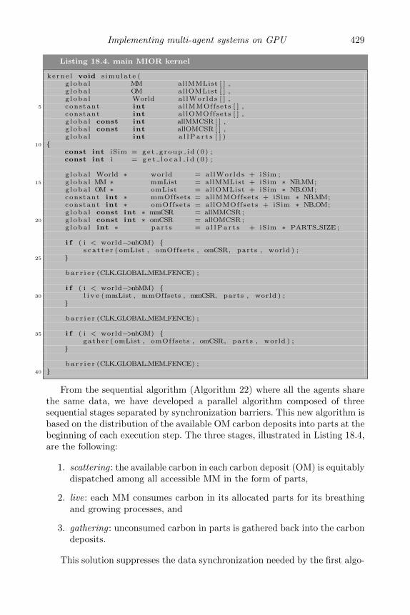
Implementing multi-agent systems on GPU 429
Listing 18.4. main MIOR kernel
ke rne l void s imulate (g l oba l MM allMMList [ ] ,g l oba l OM allOMList [ ] ,g l oba l World a l lWor lds [ ] ,
5 constant int allMMOffsets [ ] ,constant int al lOMOffsets [ ] ,g l oba l const int allMMCSR [ ] ,g l oba l const int allOMCSR [ ] ,g l oba l int a l l P a r t s [ ] )
10 const int iSim = ge t g roup id (0 ) ;const int i = g e t l o c a l i d (0 ) ;
g l oba l World ∗ world = al lWor lds + iSim ;15 g l oba l MM ∗ mmList = allMMList + iSim ∗ NB MM;
g l oba l OM ∗ omList = allOMList + iSim ∗ NB OM;constant int ∗ mmOffsets = allMMOffsets + iSim ∗ NB MM;constant int ∗ omOffsets = al lOMOffsets + iSim ∗ NB OM;g l oba l const int ∗ mmCSR = allMMCSR ;
20 g l oba l const int ∗ omCSR = allOMCSR ;g l oba l int ∗ part s = a l l P a r t s + iSim ∗ PARTS SIZE ;
i f ( i < world−>nbOM) s c a t t e r ( omList , omOffsets , omCSR, parts , world ) ;
25
b a r r i e r (CLK GLOBAL MEM FENCE) ;
i f ( i < world−>nbMM) 30 l i v e (mmList , mmOffsets , mmCSR, parts , world ) ;
b a r r i e r (CLK GLOBAL MEM FENCE) ;
35 i f ( i < world−>nbOM) gather ( omList , omOffsets , omCSR, parts , world ) ;
b a r r i e r (CLK GLOBAL MEM FENCE) ;40
From the sequential algorithm (Algorithm 22) where all the agents sharethe same data, we have developed a parallel algorithm composed of threesequential stages separated by synchronization barriers. This new algorithm isbased on the distribution of the available OM carbon deposits into parts at thebeginning of each execution step. The three stages, illustrated in Listing 18.4,are the following:
1. scattering : the available carbon in each carbon deposit (OM) is equitablydispatched among all accessible MM in the form of parts,
2. live: each MM consumes carbon in its allocated parts for its breathingand growing processes, and
3. gathering : unconsumed carbon in parts is gathered back into the carbondeposits.
This solution suppresses the data synchronization needed by the first algo-

430 Designing Scientific Applications on GPUs
rithm, thus the need for synchronization barriers, and requires only one kernellaunch from Java as described on Listing 18.5.
Listing 18.5. MIOR simulation launcher
@Overrideprotec ted void doLiveImpl ( )
s imulateKerne l . setArguments (mmMem, omMem, worldsMem , mmOffsetsMem ,omOffsetsMem , mmCSRMem, omCSRMem, partsMem ) ;
5 i f ( b l o ckS i z e < Math . max(nbOM, nbMM) ) throw new RuntimeException ("blockSize (" + blockS i z e +
") too small to execute the simulation" ) ;
10 OCLEvent event = queue . enqueue1DKernel ( s imulateKerne l , nbSim ∗blockS ize , b l o ckS i z e ) ;
OCLEvent . waitFor ( event ) ;
i f ( ! isBatchModeEnabled ( ) ) 15 queue . b lock ingReadBuf fer (mmMem, mmList , 0 , mmMem. ge tS i z e ( ) ) ;
queue . b lock ingReadBuf fer (omMem, omList , 0 , omMem. ge tS i z e ( ) ) ;queue . b lock ingReadBuf fer (worldsMem , worlds , 0 , worldsMem .
g e t S i z e ( ) ) ;
18.4.2.4 Termination detection
The termination of a MIOR simulation is reached when the model stabi-lizes and no more CO2 is produced. This termination detection can be doneon either the CPU or the GPU but it requires a global view on the systemexecution.
In the first case, when the CPU controls the GPU simulation process, thedetection is done in two steps: (1) the CPU starts the execution of a simulationstep on the GPU and (2) the CPU retrieves the GPU data and determines ifanother iteration must be launched or if the simulation has terminated. Thisapproach allows a fine-grain control over the GPU execution, but it requiresmany costly data transfers as each iteration result must be sent from the GPUto the CPU. In the case of the MIOR model these costs are mainly due to theinherent PCI-express port latencies rather than to bandwidth limitation sincedata sizes remains rather small, on the order of few dozens of Megabytes.
In the second case the termination detection is directly implemented on theGPU by checking the amount of available carbon between two iterations. TheCPU does not have any feedback while the simulation is running, but retrievesthe results once the kernel execution is finished. This approach minimizes thenumber of transfers between the CPU and the GPU.
18.4.3 Performance of MIOR implementations
In this part we present several MIOR GPU implementations using thedistribution/gathering process described in the previous section and compare

Implementing multi-agent systems on GPU 431
their performance on two distinct hardware platform, i.e., two different GPUdevices. Five incremental MIOR implementations were realized with an in-creasing level of adaptation for the algorithm: in all cases, we choose theaverage time over 50 executions as a performance indicator.
• The GPU 1.0 implementation is a direct implementation of the ex-isting algorithm and its data structures where data dependencies wereremoved, and it uses the noncompact topology representation describedin Section 18.4.2.2
• The GPU 2.0 implementation uses the previously described compactrepresentation of the topology and remains otherwise identical to theGPU 1.0 implementation.
• The GPU 3.0 implementation introduces the manual copy into local(private) memory of often-accessed global data, such as carbon parts ortopology information.
• The GPU 4.0 implementation is a variant of the GPU 1.0 implemen-tation but allows the execution of multiple simulations for each kernelexecution.
• The GPU 5.0 implementation is a multisimulation version of the GPU2.0 implementation, using the execution of multiple simulations for eachkernel execution as for GPU 4.0.
The two last implementations GPU 4.0 and GPU 5.0 illustrate the gainprovided by a better usage of the hardware resources, thanks to the driver ex-ecution overlapping capabilities. A sequential version of the MIOR algorithm,labeled CPU, is included for comparison purpose. This sequential version wasdeveloped in Java, the same language used for GPU implementations.
For these performance evaluations, two platforms are used. The first oneis representative of the kind of hardware which is available on HPC clusters.It is a cluster node dedicated to GPU computations with two Intel X5550processors running at 2.67GHz and one Tesla C1060 GPU device running at1.3GHz and composed of 240 cores (30 multiprocessors). The second platformillustrates what can be expected from a personal desktop computer built afew years ago. It uses an Intel Q9300 CPU, running at 2.5GHz, and a Geforce8800GT GPU running at 1.5GHz and composed of 112 cores (14 multiproces-sors). The purpose of these two platforms is to assess the benefit that couldbe obtained when a scientist has access either to specialized hardware as acluster or tries to take advantage of its own personal computer.
Figures 18.5 and 18.6 show the execution time for 50 simulations on thetwo hardware platforms. A size factor is applied to the problem: at scale 1, themodel contains 38 MM and 310 OM, while at the scale 6 these numbers aremultiplied by six. The size of the environment is modified as well to maintain

432 Designing Scientific Applications on GPUs
0
20
40
60
80
100
120
140
160
180
0 2 4 6 8 10
Avera
ge s
imula
tion t
ime (
ms)
Model scaling factor
CPUGPU v1.0GPU v2.0GPU v3.0
FIGURE 18.5. CPU and GPU performance on a Tesla C1060 node.
0
200
400
600
800
1000
1200
0 2 4 6 8 10
Avera
ge s
imula
tion t
ime (
ms)
Model scaling factor
CPUGPU v1.0GPU v2.0GPU v3.0
FIGURE 18.6. CPU and GPU performance on a personal computer with aGeforce 8800GT.
the same average agent density in the model. This scaling factor displays theimpact of the chosen size of simulation on performance.
The charts show that for small problems the execution times of all theimplementations are very close. This is because the GPU execution does nothave enough threads (representing agents) for an optimal usage of GPU re-sources. This trend changes around scale 5 where GPU 2.0 and GPU 3.0 takethe advantage over the GPU 1.0 and CPU implementations. This advantagecontinues to grow with the scaling factor, and reaches a speedup of 10 at the
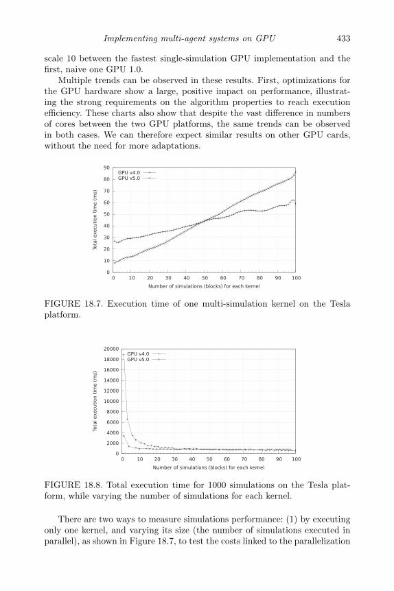
Implementing multi-agent systems on GPU 433
scale 10 between the fastest single-simulation GPU implementation and thefirst, naive one GPU 1.0.
Multiple trends can be observed in these results. First, optimizations forthe GPU hardware show a large, positive impact on performance, illustrat-ing the strong requirements on the algorithm properties to reach executionefficiency. These charts also show that despite the vast difference in numbersof cores between the two GPU platforms, the same trends can be observedin both cases. We can therefore expect similar results on other GPU cards,without the need for more adaptations.
0
10
20
30
40
50
60
70
80
90
0 10 20 30 40 50 60 70 80 90 100
Tota
l exe
cuti
on t
ime (
ms)
Number of simulations (blocks) for each kernel
GPU v4.0GPU v5.0
FIGURE 18.7. Execution time of one multi-simulation kernel on the Teslaplatform.
0
2000
4000
6000
8000
10000
12000
14000
16000
18000
20000
0 10 20 30 40 50 60 70 80 90 100
Tota
l exe
cuti
on t
ime (
ms)
Number of simulations (blocks) for each kernel
GPU v4.0GPU v5.0
FIGURE 18.8. Total execution time for 1000 simulations on the Tesla plat-form, while varying the number of simulations for each kernel.
There are two ways to measure simulations performance: (1) by executingonly one kernel, and varying its size (the number of simulations executed inparallel), as shown in Figure 18.7, to test the costs linked to the parallelization

434 Designing Scientific Applications on GPUs
process or (2) by executing a fixed number of simulations and varying the sizeof each kernel, as shown in Figure 18.8.
Figure 18.7 illustrates the execution time for only one kernel. It shows thatfor small numbers of simulations run in parallel, the compact implementationof the model topology is faster than the two-dimension matrix representation.This trends reverse with more than 50 simulations in parallel, which can beexplained either by the nonlinear progression of the synchronization costs orby the additional memory required for the access-efficient representation.
Figure 18.8 illustrates the execution time of a fixed number of simula-tions. It shows that for a small number of simulations run in parallel, thecosts resulting from program setup, data copies, and launch on GPU are verydetrimental to performance. Once the number of simulations executed for eachkernel grows, these costs are counterbalanced by computation costs. This trendis more marked in the case of the sparse implementation (GPU 4.0) than inthe compact one but appears on both curves. With more than 30 simulationsfor each kernel, execution times stall, since hardware limits are reached. Thisindicates that the cost of preparing and launching kernels become negligiblecompared to the computing time once a good GPU occupancy rate is achieved.
18.5 Analysis and recommendations
In this section we synthesize the observations done on the two models andidentify some recommendations for implementing complex systems on GPUplatforms.
18.5.1 Analysis
In both the collembola and the MIOR model, a critical problematic is thedetermination of the parts of the simulation that are to be run on GPU andwhich are to remain on the CPU. The determination of these parts is a classicstep of any algorithm parallelization and must take into account considerationssuch as the cost of the different parts of the algorithm and the expected gains.
In the case of the collembola model two steps of the algorithm were portedto GPU. Both steps use straightforward, easily parallelizable operations wherea direct gain can be expected by using more execution cores without importantmodifications to the algorithm.
In the MIOR model case, however, no such inherently parallelizable partsare evident in the original sequential algorithm. This is mainly explained bythe rate of interactions between agents in this model in the form of two oper-ations (breathing, growth) using heavily-shared carbon resources. In this casethe algorithm had to be more profoundly modified while keeping in mind theneed to remain true to the original model, to synchronize the main execution

Implementing multi-agent systems on GPU 435
step of all agents in the model, to ensure equity, and to minimize the numbersof synchronizations. The minimization is done by factoring the distribution ofcarbon in the model in two separated steps at the beginning and the end ofeach iteration rather than at multiple points of the execution.
18.5.2 MAS execution workflow
Many MAS simulations decompose their execution process into discreteevolution steps where each step represents a quantum of time (minimal unit oftime described). At the end of each step many global data, graphical displaysor output files are updated. This execution model may not correctly fit onGPU platforms as they assume more or less a batch-like workflow model. Theexecution model must be split into the following ever repeating steps:
• Allocation of GPU data buffers
• Copy of data from CPU to GPU
• GPU kernels execution
• Copy of results from GPU to CPU
This workflow works well if the considered data transfer time is negligiblecompared to GPU execution or can be done in parallel, thanks to the asyn-chronous nature of OpenCL. If we are to update the MAS model after eachiteration then performance risks being degraded. This is illustrated in theMIOR model by the fact that the speedup observed on GPU is much moresignificant for bigger simulations, which imply longer GPU execution times.Our solution to this problem is to desynchronize the execution of the MASmodel and its GPU parts by requesting the execution of multiple steps of theGPU simulations for each launch.
Another related prerequisite of GPU execution is the ability to have manythreads executed, to allow an efficient exploitation of the superior number ofcores provided by the architecture. In the case of MAS models, this means thatexecuting one agent at a time on GPU is meaningless in regard to GPU usage,copying cost, and actual gain in execution time, if the agent computations arenot complex enough. In the MIOR and the collembola models, this is solvedby executing the computations for all agents of the model at the same time. Ifthe model has only chronic needs for intensive computations, then some kindof batching mechanism is required to store waiting treatments in a queue,until the total sum of waiting computations justifies the transfer cost to theGPU platform.
18.5.3 Implementation challenges
Besides the execution strategy challenges described above, some imple-mentation challenges also occur when implementing an OpenCL version of

436 Designing Scientific Applications on GPUs
a MAS model, mainly related to the underlying limitations of the executionplatform.
The first one is the impossibility (except in latest CUDA versions) todynamically allocate memory during execution. This is a problem in the caseof models where the number of agents can vary during the simulation, suchas prey-predator models. In this case, the only solution is to overestimate thesize of arrays or data structures to accommodate these additional individuals,or to use the CPU to resize data structures when these situations occur. Bothapproaches require trending either memory or performance and are not alwayspractical.
Another limitation is the impossibility to store pointers in data structures,since OpenCL only allows one-dimension static arrays. This precludes the us-age of structures such as linked-list, graphs or sparse matrices not representedby some combination of static arrays, and can be another source of memoryor performance losses.
In the case of MIOR, this problem is especially exacerbated in the case ofneighboring storage: both representations consume much more memory thanis actually required, since the worst case (all agents have access to all othersagents) has to be taken into account when dimensioning the data structure.
The existence of different generations of GPU hardware is also a challenge.Older implementations, such as the four year old Tesla C1060 cards, havevery strong constraints in term of memory accesses and requires very regularaccess patterns to perform efficiently. MAS having many random accesses,such as MIOR, or many small global memory accesses, such as Collembola,are penalized on these older cards. Fortunately, these requirements are lesspresent is modern cards, which offer caches and other facilities traditionallypresent on CPU to offset these kinds of penalties.
The final concern is related to the previous ones and often results in morememory consumption. The amount of memory available on GPU cards is muchmore limited and adding new memory capabilities is more costly compared toexpending a CPU RAM. On computing clusters, hardwares nodes with 128GBof memory or more have become affordable, whereas newer Tesla architectureremains limited to 16GB of memory. This can be a concern in the case of bigMAS models, or small ones which can only use memory-inefficient OpenCLstructures.
18.5.4 MCSMA
As shown in the previous sections, many data representation choices arecommon to entire classes of MAS. The paradigm of grid, for example, is oftenencountered in models where each cell constitutes either the elementary unitof simulation (SugarScape [10]) or a discretization of the environment space(Pathfinding [13]). These grids can be considered as two- or three-dimensionalmatrices, whose processing can be directly distributed.
Another common data representation encountered in MAS system is the

Implementing multi-agent systems on GPU 437
usage of 2D or 3D coordinates to store the position of each agent of themodel. In this case, even if the environment is no longer discrete, the loca-tion information still imply computations (Euclidean distances) which can beparallelized.
MCSMA [16] is a framework developed to provide to the MAS designerthose basic data structures and the associated operations, to facilitate theportage of existing MAS on GPU. Two levels of utilization are provided tothe developer, depending on its usage profile:
• A high-level library, composed of modules regrouping classes of opera-tions. Such operation can distance computations in 1D, 2D or 3D grids,diffusion or reduction operations on matrices...
• A low-level API which allows the developer direct access to the GPUand the inner working of MCSMA, to develop new modules in the casewhere the required operations are not yet provided by the platform.
Both usage levels were illustrated in the above two practical cases. InMIOR, the whole algorithm (baring initialization) is ported on GPU as a spe-cific plugin which allows executing n MIOR simulations and retrieving theirresults. This first approach requires extensive adaptations to the original algo-rithm. In collembola, to the contrary, the main steps of the algorithm remainexecuted on the CPU, and only specific operations are delegated to generic,already existing diffusion and reduction kernels. The fundamental algorithmis not modified and GPU execution is only applied to specific parts of the ex-ecution which may benefit from it. These two programming approaches allowincremental adaptations of existing Java MAS to accelerate their executionon GPU, while retaining the option to develop their own reusable or moreefficient module to supplement the already existing ones.
18.6 Conclusion
This chapter has addressed the issue of complex system simulation by usingagent-based paradigms and GPU hardware. From the experiments on twoexisting agent-based models of soil science we have provided useful informationon the architecture, the algorithm design, and the data management to runagent-based simulations on GPU, and more generally to run computationallyintensive applications that are not based on purely-matricial models. The firstresult of this work is that adapting the algorithm to a GPU architecture ispossible and suitable to speed up agent based simulations as illustrated by theMIOR model. Coupling CPU with GPU seems to be an interesting way to takebetter advantage of the power given by computers and clusters as illustratedby the collembola model. From our point of view the adaptation process is less

438 Designing Scientific Applications on GPUs
costy in time than a traditional parallelization on distributed nodes and notmuch difficult than a standard multithreaded parallelization, since all the dataremains on the same host and can be shared in central memory. The usageof OpenCL also enables a portable simulator that can be run on differentgraphical units. Even using a mainstream card such as the GPU card of astandard computer can lead to significant performance improvements. This isan interesting result as it opens up the field of inexpensive HPC to a largecommunity.
In this perspective, we are working on MCSMA, a development platformthat would facilitate the use of GPU or many-core architectures for multi-agent simulations. Our first work has been the definition of common, efficient,reusable data structures, such as grids or lists. Another goal is to provide easiermeans to control the distribution of specific processes between CPU or GPU,to allow the easy exploitation of the strengths of each platform in the samemulti-agent simulation. We think that the same approach, i.e., developingspecific environments that facilitate the developer access to the GPU power,can be applied in many domains with computationally intensive needs to openthe GPU use to a larger community.
Bibliography
[1] JOCL: Java Bindings for OpenCL. http://www.jocl.org.
[2] B. G. Aaby, K. S. Perumalla, and S. K. Seal. Efficient simulation of agent-based models on multi-GPU and multi-core clusters. In Proceedings of the3rd International ICST Conference on Simulation Tools and Techniques,SIMUTools ’10, pages 29:1–29:10, ICST, Brussels, Belgium, 2010. ICST(Institute for Computer Sciences, Social-Informatics and Telecommuni-cations Engineering).
[3] E. Blanchart, C. Cambier, C. Canape, B. Gaudou, T.-N. Ho, T.-V. Ho,C. Lang, F. Michel, N. Marilleau, and L. Philippe. EPIS: A grid plat-form to ease and optimize multi-agent simulators running. In PAAMS,volume 88 of Advances in Intelligent and Soft Computing, pages 129–134,Salamanca, Spain, 2011. Springer.
[4] A. Bleiweiss. Multi agent navigation on the GPU. GDC09 Game Devel-opers Conference, 2099.
[5] C. Cambier, D. Masse, M. Bousso, and E. Perrier. An offer versus de-mand modelling approach to assess the impact of micro-organisms spatio-temporal dynamics on soil organic matter decomposition rates. EcologicalModelling, pages 301–313, 2007.

Implementing multi-agent systems on GPU 439
[6] F. Chuffart, N. Dumoulin, T. Faure, and G. Deffuant. Simexplorer: Pro-gramming experimental designs on models and managing quality of mod-elling process. IJAEIS, 1(1):55–68, 2010.
[7] N.T. Collier and M.J North. Repast SC++: A Platform for Large-scaleAgent-based Modeling, chapter Large-Scale Computing Techniques forComplex System Simulation. Wiley (In Press), 2011.
[8] B. Cosenza, G. Cordasco, R. De Chiara, and V. Scarano. Distributed loadbalancing for parallel agent-based simulations. In 19th Euromicro Inter-national Conference on Parallel, Distributed and Network-Based Com-puting, pages 62–69, Ayia Napa, Cyprus, 2011.
[9] T. Da Silva Joao Luis and Y. Demazeau. Vowels co-ordination model. InAAMAS, pages 1129–1136, Bologna, Italy, 2002.
[10] Rahmani K. D’Souza R. M., Lysenko M. SugarScape on steroids: Sim-ulating over a million agents at interactive rates. In Proceedings of theAgent 2007 Conference, Chicago, USA, 2007.
[11] J. Gomez-Luna, J.-M. Gonzalez-Linares, J.-I. Benavides, and N. Guil.Parallelization of a video segmentation algorithm on CUDA-enabledgraphics processing units. In 15th Euro-Par Conference, pages 924–935,Berlin, Heidelberg, 2009. Springer-Verlag.
[12] O. Gutknecht and J. Ferber. Madkit: a generic multi-agent platform.In Proceedings of the Fourth International Conference on AutonomousAgents, AGENTS ’00, pages 78–79, New York, NY, USA, 2000. ACM.
[13] S. J. Guy, J. Chhugani, C. Kim, N. Satish, M. C. Lin, D. Manocha, andP. Dubey. Clearpath: highly parallel collision avoidance for multi-agentsimulation. In ACM Siggraph/Eurographics Symposium on ComputerAnimation, pages 177–187, New Orleans, LA, USA, 2009. ACM.
[14] M. Kiran, P. Richmond, M. Holcombe, L. S. Chin, D. Worth, and C. Gree-nough. Flame: simulating large populations of agents on parallel hard-ware architectures. In Proceedings of the 9th International Conferenceon Autonomous Agents and Multiagent Systems, volume 1, AAMAS,pages 1633–1636, Richland, SC, 2010. International Foundation for Au-tonomous Agents and Multiagent Systems.
[15] G. Laville, K. Mazouzi, C. Lang, N. Marilleau, and L. Philippe. Us-ing GPU for multi-agent multi-scale simulations. In DCAI’12, 9-th Int.Conf. on Advances in Intelligent and Soft Computing, volume 151 ofAdvances in Intelligent and Soft Computing, pages 197–204, Salamanca,Spain, March 2012. Springer.

440 Designing Scientific Applications on GPUs
[16] G. Laville, K. Mazouzi, C. Lang, N. Marilleau, and L. Philippe. UsingGPU for multi-agent soil simulation. In PDP 2013, 21st Euromicro In-ternational Conference on Parallel, Distributed and Network-based Com-puting, pages 392–399, Belfast, Ireland, February 2013. IEEE ComputerSociety Press.
[17] O. Maitre, N. Lachiche, P. Clauss, L. Baumes, A. Corma, and P. Collet.Efficient parallel implementation of evolutionary algorithms on GPGPUcards. In Henk Sips, Dick Epema, and Hai-Xiang Lin, editors, Euro-Par 2009 Parallel Processing, volume 5704 of Lecture Notes in ComputerScience, pages 974–985. Springer Berlin / Heidelberg, 2009. 10.1007/978-3-642-03869-3
[18] N. Marilleau, C. Lang, P. Chatonnay, and L. Philippe. An agent basedframework for urban mobility simulation. In PDP, pages 355–361,Montbeliard, France, 2006. IEEE Computer Society.
[19] M. J. North, T. R. Howe, N. T. Collier, and J. R. Vos. A declarative modelassembly infrastructure for verification and validation. In Springer, edi-tor, Advancing Social Simulation: The First World Congress, Heidelberg,FRG, 2007.
[20] J. J. Odell, H. Van Dyke Parunak, and M. Fleischer. The role of rolesin designing effective agent organizations. In Alessandro Garcia, CarlosLucena, Franco Zambonelli, Andrea Omicini, and Jaelson Castro, editors,Software engineering for large-scale multi-agent systems, pages 27–38.Springer-Verlag, Berlin, Heidelberg, 2003.
[21] F. Schweitzer and J. D. Farmer. Brownian Agents and Active Particles:Collective Dynamics in the Natural and Social Sciences. Complexity.Springer, 2003.
[22] L. Sean, C. Cioffi-Revilla, L. Panait, K. Sullivan, and G. Balan. MASON:A multi-agent simulation environment. Simulation: Transactions of thesociety for Modeling and Simulation International, 82(7):517–527, 2005.
[23] R. Silveira, L. Fischer, J. A. S. Ferreira, E. Prestes, and L. Nedel. Path-planning for RTS games based on potential fields. In Proceedings ofthe Third International Conference on Motion in Games, MIG’10, pages410–421, Berlin, Heidelberg, 2010. Springer-Verlag.
[24] E. Sklar. NetLogo, a multi-agent simulation environment. Artificial Life,13(3):303–311, 2011.
[25] David Strippgen and Kai Nagel. Multi-agent traffic simulation withCUDA. International Conference on High Performance Computing Sim-ulation, pages 106–114, 2009.

Chapter 19
Pseudorandom number generator onGPU
Raphael Couturier and Christophe Guyeux
Femto-ST Institute, University of Franche-Comte, France
19.1 Introduction . . . . . . . . . . . . . . . . . . . . . . . . . . . . . . . . . . . . . . . . . . . . . . . . . . . . . . 44119.2 Basic reminders . . . . . . . . . . . . . . . . . . . . . . . . . . . . . . . . . . . . . . . . . . . . . . . . . . 443
19.2.1 A short presentation of chaos . . . . . . . . . . . . . . . . . . . . . . . . . . . 44319.2.2 On Devaney’s definition of chaos . . . . . . . . . . . . . . . . . . . . . . . . 44319.2.3 Chaotic iterations . . . . . . . . . . . . . . . . . . . . . . . . . . . . . . . . . . . . . . . . 444
19.3 Toward efficiency and improvement for CI PRNG . . . . . . . . . . . . . . 44519.3.1 First efficient implementation of a PRNG based on
chaotic iterations . . . . . . . . . . . . . . . . . . . . . . . . . . . . . . . . . . . . . . . . 44519.3.2 Efficient PRNGs based on chaotic iterations on GPU . . 44619.3.3 Naive version for GPU . . . . . . . . . . . . . . . . . . . . . . . . . . . . . . . . . . 44619.3.4 Improved version for GPU . . . . . . . . . . . . . . . . . . . . . . . . . . . . . . 44719.3.5 Chaos evaluation of the improved version . . . . . . . . . . . . . . . 448
19.4 Experiments . . . . . . . . . . . . . . . . . . . . . . . . . . . . . . . . . . . . . . . . . . . . . . . . . . . . . . 44919.5 Summary . . . . . . . . . . . . . . . . . . . . . . . . . . . . . . . . . . . . . . . . . . . . . . . . . . . . . . . . . 450
Bibliography . . . . . . . . . . . . . . . . . . . . . . . . . . . . . . . . . . . . . . . . . . . . . . . . . . . . . . 450
19.1 Introduction
Randomness is of importance in many fields such as scientific simulationsor cryptography. Random numbers can mainly be generated by either a deter-ministic and reproducible algorithm called a pseudorandom number generator(PRNG), or by a physical nondeterministic process having all the character-istics of a random noise, called a truly random number generator (TRNG). Inthis chapter, we focus on reproducible generators, useful for instance in MonteCarlo-based simulators. These domains need PRNGs that are statistically ir-reproachable. In some fields such as in numerical simulations, speed is a strongrequirement that is usually attained by using parallel architectures. In thatcase, a recurrent problem is that a deflation of the statistical qualities is oftenreported, when the parallelization of a good PRNG is realized. This is why
441

442 Designing Scientific Applications on GPUs
ad hoc PRNGs for each possible architecture must be found to achieve bothspeed and randomness. On the other hand, speed is not the main requirementin cryptography: the most important point is to define secure generators ableto withstand malicious attacks. Roughly speaking, an attacker should not beable in practice to make the distinction between numbers obtained with thesecure generator and a true random sequence. Or, in an equivalent formula-tion, he or she should not be able (in practice) to predict the next bit of thegenerator, having the knowledge of all the binary digits that have been alreadyreleased [9]. “Being able in practice” refers here to the possibility to achievethis attack in polynomial time and to the exponential growth of the difficultyof this challenge when the size of the parameters of the PRNG increases.
Finally, a small part of the community working in this domain focuses ona third requirement: to define chaotic generators [8, 11, 17]. The main idea isto benefit from a chaotic dynamical system to obtain a generator that is un-predictable, disordered, sensible to its seed, or in other words, chaotic. Thesescientists’ desire is to map a given chaotic dynamics into a sequence that seemsrandom and unassailable due to chaos. However, the chaotic maps used as apattern are defined in the real line whereas computers deal with finite preci-sion numbers. This distortion leads to a deflation of both chaotic propertiesand speed. Furthermore, authors of such chaotic generators often claim theirPRNG as secure due to their chaos properties, but there is no obvious relationbetween chaos and security as it is understood in cryptography. This is whythe use of chaos for PRNG still remains marginal and disputable. However,we have established in previous researches that these flaws can be circum-vented by using a tool called choatic iterations. Such investigations have ledto the definition of a new family of PRNGs that are chaotic while being fastand statistically perfect, or cryptographically secure [1, 2, 5, 6]. This family isimproved and adapted for GPU architectures in this chapter.
Let us finish this introduction by noticing that, in this chapter, statisticalperfection refers to the ability to pass the whole BigCrush battery of tests,which is widely considered as the most stringent statistical evaluation of asequence claimed as random. This battery can be found in the well-knownTestU01 package [12]. More precisely, each time we performed a test on aPRNG, we ran it twice in order to observe if all p-values were inside [0.01,0.99]. In fact, we observed that few p-values (fewer than 10 out of 160) aresometimes outside this interval but inside [0.001, 0.999], so that is why asecond run has allowed us to confirm that the values outside are not for thesame test. With this approach all our PRNGs pass the BigCrush successfullyand all p-values are at least once inside [0.01, 0.99]. Chaos, for its part, refersto the well-established definition of a chaotic dynamical system defined byDevaney [7].
The remainder of this chapter is organized as follows. Basic definitions andterminologies about both topological chaos and chaotic iterations are providedin the next section. Various chaotic iterations based on pseudorandom numbergenerators are then presented in Section 19.3. They encompass naive and

Pseudorandom number generator on GPU 443
improved efficient generators for CPU and for GPU. These generators arefinally experimented in Section 19.4.
19.2 Basic reminders
This section is devoted to basic definitions and terminologies in the fieldsof topological chaos and chaotic iterations. We assume the reader is familiarwith basic notions on topology (see for instance [7]).
19.2.1 A short presentation of chaos
Chaos theory studies the behavior of dynamical systems that are perfectlypredictable, yet appear to be wildly amorphous and meaningless. Chaoticsystems are highly sensitive to initial conditions, which is popularly referredto as the butterfly effect. In other words, small differences in initial conditions(such as those due to rounding errors in numerical computation) yield widelydiverging outcomes, in general rendering long-term prediction impossible [11].This happens even though these systems are deterministic, meaning that theirfuture behavior is fully determined by their initial conditions, with no randomelements involved [11]. That is, the deterministic nature of these systems doesnot make them predictable [11, 16]. This behavior is known as deterministicchaos, or simply chaos. It has been well-studied in mathematics and physics,leading among other things to the well-established definition of Devaney whichcan be found next.
19.2.2 On Devaney’s definition of chaos
Consider a metric space (X , d) and a continuous function f : X −→ X , forone-dimensional dynamical systems of the form:
x0 ∈ X and ∀n ∈ N∗, xn = f(xn−1), (19.1)
the following definition of chaotic behavior, formulated by Devaney [7], iswidely accepted.
Definition 1 A dynamical system of Form (19.1) is said to be chaotic if thefollowing conditions hold.
• Topological transitivity:
∀U, V open sets of X , ∃k > 0, fk(U) ∩ V 6= ∅. (19.2)
Intuitively, a topologically transitive map has points that eventually move

444 Designing Scientific Applications on GPUs
under iteration from one arbitrarily small neighborhood to any other.Consequently, the dynamical system cannot be decomposed into two dis-joint open sets that are invariant under the map. Note that if a mappossesses a dense orbit, then it is clearly topologically transitive.
• Density of periodic points in X :
Let P = p ∈ X |∃n ∈ N∗ : fn(p) = p the set of periodic points of f .Then P is dense in X :
P = X . (19.3)
The density of periodic orbits means that every point in space is closelyapproached by periodic orbits in an arbitrary way. Topologically mix-ing systems failing this condition may not display sensitivity to initialconditions presented below and, hence,may not be chaotic.
• Sensitive dependence on initial conditions:
∃ε > 0, ∀x ∈ X , ∀δ > 0, ∃y ∈ X , ∃n ∈ N, d(x, y) < δ andd(fn(x), fn(y)
)> ε.
Intuitively, a map possesses sensitive dependence on initial conditionsif there exist points arbitrarily close to x that eventually separate fromx by at least ε under the iteration of f . Not all points near x need tobe eventually separate from x under iteration, but there must be at leastone such point in every neighborhood of x. If a map possesses sensi-tive dependence on initial conditions, then for all practical purposes, thedynamics of the map defy numerical computation. Small errors in com-putation that are introduced by round-off may become magnified uponiteration. The results of numerical computation of an orbit, no matterhow accurate, may bear no resemblance whatsoever with the real orbit.
When f is chaotic, then the system (X , f) is chaotic and quoting De-vaney [7, p. 50]: “it is unpredictable because of the sensitive dependence oninitial conditions. It cannot be broken down or decomposed into two subsys-tems which do not interact because of topological transitivity. And, in themidst of this random behavior, we nevertheless have an element of regular-ity.” Fundamentally different behaviors are consequently possible and occurin an unpredictable way.
19.2.3 Chaotic iterations
Let us now introduce an example of a dynamical systems family that hasthe potentiality to become chaotic, depending on the choice of the iterationfunction. This family is the basis of the PRNGs we will develop during thischapter.

Pseudorandom number generator on GPU 445
Definition 2 The set B denoting 0, 1, let f : BN −→ BN be an “iteration”function and S be a sequence of subsets of J1,NK called a chaotic strategy.Then, the so-called chaotic iterations are defined by [15]:
x0 ∈ BN,
∀n ∈ N∗,∀i ∈ J1;NK, xni =
xn−1i if i /∈ Snf(xn−1)i if i ∈ Sn.
(19.4)
In other words, at the nth iteration, only the cells of Sn are iterated.Chaotic iterations generate a set of vectors; they are defined by an initialstate x0, an iteration function f , and a chaotic strategy S [3]. These “chaoticiterations” can behave chaotically as defined by Devaney, depending on thechoice of f [3]. For instance, chaos is obtained when f is the vectorial negation.Note that, with this example of function, chaotic iterations defined above canbe rewritten as
x0 ∈ J0, 2N − 1K, Sn ∈ P(J1, 2N − 1K
)N, xn+1 = xn ⊕ Sn, (19.5)
where P(X) stands for the set of subsets of X, whereas a ⊕ b is the bitwiseexclusive or operation between the binary representation of the integers a andb. Note that the term Sn is directly and obviously linked to the Sn of Eq. 19.4.Such an iterative sequence satisfies the Devaney’s definition of chaos.
19.3 Toward efficiency and improvement for CI PRNG
19.3.1 First efficient implementation of a PRNG based onchaotic iterations
Listing 19.1. C code of the sequential PRNG based on chaotic iterations
unsigned int CIPRNG()
stat ic unsigned int x = 123123123;unsigned long t1 = x o r s h i f t ( ) ;
5 unsigned long t2 = xor128 ( ) ;unsigned long t3 = xorwow ( ) ;x = xˆ(unsigned int ) t1 ;x = xˆ(unsigned int ) ( t2>>32) ;x = xˆ(unsigned int ) ( t3>>32) ;
10 x = xˆ(unsigned int ) t2 ;x = xˆ(unsigned int ) ( t1>>32) ;x = xˆ(unsigned int ) t3 ;return x ;

446 Designing Scientific Applications on GPUs
In Listing 19.1 a sequential version of the proposed PRNG based on chaoticiterations is presented, which extends the generator family formerly presentedin [4,5]. The xor operator is represented by ˆ. This function uses three classical64-bit PRNGs, namely the xorshift, the xor128, and the xorwow [13].In the following, we call them “xor-like PRNGs”. As each xor-like PRNGuses 64-bits whereas our proposed generator works with 32-bits, we use thecommand (unsigned int), which selects the 32 least significant bits of agiven integer, and the code (unsigned int)(t>>32) in order to obtainthe 32 most significant bits of t.
Thus producing a pseudorandom number needs 6 xor operations with 6 32-bit numbers that are provided by 3 64-bit PRNGs. This version successfullypasses the stringent BigCrush battery of tests [12]. At this point, we havedefined an efficient and statistically unbiased generator. Its speed is directlyrelated to the use of linear operations, but for the same reason, this fastgenerator cannot be proven as secure.
19.3.2 Efficient PRNGs based on chaotic iterations on GPU
In order to benefit from the computing power of GPU, a program needsto have independent blocks of threads that can be computed simultaneously.In general, the larger the number of threads is, the more local memory isused, and the less branching instructions are used (if, while, etc.) and so, thebetter the performances on GPU are. Obviously, having these requirementsin mind, it is possible to build a program similar to the one presented inListing 19.1, which computes pseudorandom numbers on GPU. To do so, wemust first recall that in the CUDA [14] environment, threads have a localidentifier called ThreadIdx, which is relative to the block containing them.Furthermore, in CUDA, parts of the code that are executed by the GPU arecalled kernels.
19.3.3 Naive version for GPU
It is possible to deduce from the CPU version a quite similar versionadapted to GPU. The simple principle consists of making each thread of theGPU compute the CPU version of our PRNG. Of course, the three xor-likePRNGs used in these computations must have different parameters. In a giventhread, these parameters are randomly picked from another PRNGs. The ini-tialization stage is performed by the CPU. To do this, the Indirection, Shift,Accumulate, Add, and Count (ISAAC) PRNG [10] is used to set all the pa-rameters embedded into each thread.
The implementation of the three xor-like PRNGs is straightforward whentheir parameters have been allocated in the GPU memory. Each xor-like workswith an internal number x that saves the last generated pseudorandom num-ber. Additionally, the implementation of the xor128, the xorshift, and thexorwow, respectively, require 4, 5, and 6 unsigned long as internal variables.

Pseudorandom number generator on GPU 447
Algorithm 23: main kernel of the GPU “naive” version of the PRNGbased on chaotic iterations
Input: InternalVarXorLikeArray: array with internal variables of the 3xor-like PRNGs in global memory;
NumThreads: number of threads;Output: NewNb: array containing random numbers in global memory
1 if threadIdx is concerned by the computation then2 retrieve data from InternalVarXorLikeArray[threadIdx] in local variables;3 for i=1 to n do4 compute a new PRNG as in Listing 19.1;5 store the new PRNG in NewNb[NumThreads*threadIdx+i];
6 end7 store internal variables in InternalVarXorLikeArray[threadIdx];
8 end
Algorithm 23 presents a naive implementation of the proposed PRNG onGPU. Due to the available memory in the GPU and the number of threadsused simultaneously, the number of random numbers that a thread can gener-ate inside a kernel is limited (i.e., the variable n in Algorithm 23). For instance,if 100, 000 threads are used and if n = 1001, then the memory required to storeall of the internal variables of both the xor-like PRNGs2 and the pseudoran-dom numbers generated by our PRNG, is equal to 100, 000 × ((4 + 5 + 6) ×2 + (1 + 100)) = 1, 310, 000 32-bit numbers, that is, approximately 52Mb.
This generator is able to pass the whole BigCrush battery of tests, for allthe versions that have been tested depend on their number of threads (calledNumThreads in our algorithm, tested up to 5 million).
19.3.4 Improved version for GPU
As GPU cards using CUDA have shared memory between threads of thesame block, it is possible to use this feature in order to simplify the previousalgorithm, i.e., to use fewer than 3 xor-like PRNGs. The solution consistsin computing only one xor-like PRNG by thread, saving it into the sharedmemory, and then using the results of some other threads in the same blockof threads. In order to define which thread uses the result of which other one,we can use a combination array that contains the indexes of all threads andfor which a combination has been performed.
In Algorithm 24, two combination arrays are used. The variable offset iscomputed using the value of combination size. Then we can compute o1 ando2 representing the indexes of the other threads whose results are used by thecurrent one. In this algorithm, we consider that a 32-bit xor-like PRNG has
1In fact, we need to add the initial seed (a 32-bit number).2We multiply this number by 2 in order to count 32-bit numbers.

448 Designing Scientific Applications on GPUs
been chosen. In practice, we use the xor128 proposed in [13] in which unsignedlongs (64 bits) have been replaced by unsigned integers (32 bits).
This version can also pass the whole BigCrush battery of tests.
Algorithm 24: main kernel for the chaotic iterations based PRNG GPUefficient version
Input: InternalVarXorLikeArray: array with internal variables of 1 xor-likePRNGs in global memory;
NumThreads: Number of threads;array comb1, array comb2: Arrays containing combinations of sizecombination size;Output: NewNb: array containing random numbers in global memory
1 if threadId is concerned then2 retrieve data from InternalVarXorLikeArray[threadIdx] in local variables
including shared memory and x;3 offset = threadIdx%combination size;4 o1 = threadIdx-offset+array comb1[offset];5 o2 = threadIdx-offset+array comb2[offset];6 for i=1 to n do7 t=xor-like();8 t=tˆshmem[o1]ˆshmem[o2];9 shared mem[threadId]=t;
10 x = xˆt;11 store the new PRNG in NewNb[NumThreads*threadIdx+i];
12 end13 store internal variables in InternalVarXorLikeArray[threadIdx];
14 end
19.3.5 Chaos evaluation of the improved version
A run of Algorithm 24 consists of an operation (x = x⊕ t) having the formof Equation 19.5, which is equivalent to the iterative system of Eq. 19.4. Thatis, an iteration of the general chaotic iterations is realized between the laststored value x of the thread and a strategy t (obtained by a bitwise exclusiveor between a value provided by a xor-like() call and two values previouslyobtained by two other threads). To be certain that such iterations correspondto the chaotic one recalled at the end of Section 19.2.2, we must guarantee that
this dynamical system iterates on the space X = BN × P(J1, 2NK
)N. The left
term x obviously belongs to BN. To prevent any flaws of chaotic properties,we must check that the right term (the last t in Algorithm 24), correspondingto the strategies, can possibly be equal to any integer of J1, 2NK.
Such a result is obvious; as for the xor-like(), all the integers belongingto its interval of definition can occur at each iteration, and thus the last trespects the requirement. Furthermore, it is possible to prove by an imme-diate mathematical induction that, supposing that the initial x is uniformly

Pseudorandom number generator on GPU 449
distributed, the two other stored values shmem[o1] and shmem[o2] are uni-formly distributed too (this is the induction hypothesis), and thus the next xis finally uniformly distributed.
Thus Algorithm 24 is a concrete realization of the general chaotic iterationspresented previously, and for this reason, it satisfies the Devaney’s formulationof chaotic behavior.
19.4 Experiments
Different experiments have been performed in order to measure the genera-tion speed. We have used one computer equipped with a Tesla C1060 NVIDIAGPU card and an Intel Xeon E5530 cadenced at 2.40 GHz, and a second com-puter equipped with a smaller CPU and a GeForce GTX 280. All the cardshave 240 cores.
1e+09
1e+10
1e+11
10000 100000 1e+06 1e+07
Random
num
bers
genera
ted / s
econd
Number of threads used by the GPU
optimized PRNG on C1060optimized PRNG on GTX285
naive PRNG on C1060naive PRNG on GTX285
FIGURE 19.1. Quantity of pseudorandom numbers generated per second withthe xorlike-based PRNG.
In Figure 19.1 we compare the quantity of pseudorandom numbers gen-erated per second with various xor-like based PRNGs. In this figure, the op-timized versions use the xor64 described in [13], whereas the naive versions

450 Designing Scientific Applications on GPUs
embed the three xor-like PRNGs described in Listing 19.1. In order to obtainthe optimal performances, the storage of pseudorandom numbers to the GPUmemory has been removed. This step is time-consuming and slows down thenumbers generation. Moreover this storage is completely useless, in case of ap-plications that consume the pseudorandom numbers directly after they havebeen generated. We can see that when the number of threads is greater thanapproximately 30,000 and less than 5 million, the number of pseudorandomnumbers generated per second is almost constant. With the naive version,this value ranges from 2.5 to 3GSamples/s. With the optimized version, it isapproximately equal to 20GSamples/s. Finally we can remark that both GPUcards are quite similar, but in practice, the Tesla C1060 has more memorythan the GTX 280, and this memory should be of better quality. As a com-parison, Listing 19.1 leads to the generation of about 138MSample/s whenusing one core of the Xeon E5530.
These experiments allow us to conclude that it is possible to generate avery large quantity of pseudorandom numbers statistically perfect with thexor-like version.
19.5 Summary
In this chapter, a PRNG based on chaotic iterations is presented. It isproven to be chaotic according to Devaney. Efficient implementations on GPUusing xor-like PRNGs as input generators have shown that a very large quan-tity of pseudorandom numbers can be generated per second (about 20Gsam-ples/s on a Tesla C1060), and that these proposed PRNGs succeed in passingthe hardest battery in TestU01, namely, the BigCrush.
Bibliography
[1] J. Bahi, X. Fang, and C. Guyeux. An optimization technique on pseudo-random generators based on chaotic iterations. In INTERNET’2012, 4thInt. Conf. on Evolving Internet, pages 31–36, Venice, Italy, June 2012.
[2] J. Bahi, X. Fang, C. Guyeux, and Q. Wang. Evaluating quality of chaoticpseudo-random generators. application to information hiding. IJAS, In-ternational Journal On Advances in Security, 4(1-2):118–130, 2011.
[3] J. Bahi and C. Guyeux. Hash functions using chaotic iterations. Journalof Algorithms and Computational Technology, 4(2):167–181, 2010.

Pseudorandom number generator on GPU 451
[4] J. Bahi and C. Guyeux. Topological chaos and chaotic iterations, appli-cation to hash functions. Neural Networks (IJCNN2010), pages 1–7, July2010.
[5] J Bahi, C. Guyeux, and Q. Wang. A novel pseudo-random generatorbased on discrete chaotic iterations. In INTERNET’09, 1-st Int. Conf.on Evolving Internet, pages 71–76, Cannes, France, August 2009.
[6] J. Bahi, C. Guyeux, and Q. Wang. A pseudo random numbers generatorbased on chaotic iterations. application to watermarking. In WISM 2010,Int. Conf. on Web Information Systems and Mining, volume 6318 ofLNCS, pages 202–211, Sanya, China, October 2010.
[7] R. L. Devaney. An Introduction to Chaotic Dynamical Systems. Addison-Wesley, Redwood City, CA, 2nd edition, 1989.
[8] J. Gleick. Chaos: Making a New Science. Open Road, 2011.
[9] O. Goldreich. Foundations of Cryptography: Basic Tools. CambridgeUniversity Press, 2007.
[10] R. J. Jenkins. ISAAC. In IWFSE: International Workshop on FastSoftware Encryption, volume 1039 of Lecture Notes in Computer Science,pages 41–49. Springer Verlag, 1996.
[11] S. H. Kellert. In the Wake of Chaos: Unpredictable Order in DynamicalSystems. Science and Its Conceptual Foundations. University of ChicagoPress, 1994.
[12] P. L’Ecuyer and R. J. Simard. TestU01: A C library for empirical testingof random number generators. ACM Trans. Math. Softw, 33(4):22–40,2007.
[13] G. Marsaglia. Xorshift rngs. Journal of Statistical Software, 8(14):1–6,2003.
[14] NVIDIA. CUDA CUBLAS library, 2011. Version 4.0.
[15] F. Robert. Discrete Iterations: A Metric Study, volume 6 of SpringerSeries in Computational Mathematics. 1986.
[16] C. Werndl. What are the new implications of chaos for unpredictability?The British Journal for the Philosophy of Science, 60(1):195–220, 2009.
[17] C. Wu, Z. Xu, W. Lin, and J. Ruan. Stochastic Properties in Devaney’sChaos. Chaos, Solitons and Fractals, 23(4):1195 – 1199, 2005.

This page intentionally left blankThis page intentionally left blank

Chapter 20
Solving large sparse linear systems forinteger factorization on GPUs
Bertil Schmidt and Hoang-Vu Dang
Johannes Gutenberg University of Mainz, Germany
20.1 Introduction . . . . . . . . . . . . . . . . . . . . . . . . . . . . . . . . . . . . . . . . . . . . . . . . . . . . . . 45320.2 Block Wiedemann algorithm . . . . . . . . . . . . . . . . . . . . . . . . . . . . . . . . . . . . . 45420.3 SpMV over GF(2) for NFS matrices using existing formats on
GPUs . . . . . . . . . . . . . . . . . . . . . . . . . . . . . . . . . . . . . . . . . . . . . . . . . . . . . . . . . . . . 45520.4 A hybrid format for SpMV on GPUs . . . . . . . . . . . . . . . . . . . . . . . . . . . . 459
20.4.1 Dense format . . . . . . . . . . . . . . . . . . . . . . . . . . . . . . . . . . . . . . . . . . . . 45920.4.2 Sliced COO . . . . . . . . . . . . . . . . . . . . . . . . . . . . . . . . . . . . . . . . . . . . . . 46020.4.3 Determining the cut-off point of each format . . . . . . . . . . . 464
20.5 SCOO for single-precision floating-point matrices . . . . . . . . . . . . . . . 46520.6 Performance evaluation . . . . . . . . . . . . . . . . . . . . . . . . . . . . . . . . . . . . . . . . . . 466
20.6.1 Experimental setup . . . . . . . . . . . . . . . . . . . . . . . . . . . . . . . . . . . . . . 46620.6.2 Experimental results of SpMV on NFS matrix . . . . . . . . . 46620.6.3 Experimental results of SpMV on floating-point
matrices . . . . . . . . . . . . . . . . . . . . . . . . . . . . . . . . . . . . . . . . . . . . . . . . . . 46720.6.3.1 Performance comparison to existing GPU
formats . . . . . . . . . . . . . . . . . . . . . . . . . . . . . . . . . . . . . 46720.6.3.2 Performance comparison to a CPU
implementation . . . . . . . . . . . . . . . . . . . . . . . . . . . . 46920.7 Conclusion . . . . . . . . . . . . . . . . . . . . . . . . . . . . . . . . . . . . . . . . . . . . . . . . . . . . . . . . 470
Bibliography . . . . . . . . . . . . . . . . . . . . . . . . . . . . . . . . . . . . . . . . . . . . . . . . . . . . . . 471
20.1 Introduction
The Number Field Sieve (NFS) is the current state-of-the-art integer fac-torization method. It requires the solution of a large sparse linear system overGalois Field GF(2) (called the linear algebra step). The Block Wiedemann(BW) [8] algorithm can be used to solve such a large sparse linear systemefficiently using iterative sparse matrix vector multiplication (SpMV).
Recent integer factorization efforts have been using CPU clusters to solve
453

454 Designing Scientific Applications on GPUs
the large sparse linear system [1, 17]. The RSA-768 factorization [17], for ex-ample, reported a runtime of 3 months for the linear algebra step on a clusterwith 48 AMD dual hex-core CPUs. Previous work on parallelizing the linearalgebra step focused on using CPU clusters and grids [2, 11, 12, 18]. In thischapter, we present a CUDA approach that can be used to accelerate thecostly iterative SpMV operation for matrices derived from NFS.
The memory access pattern in the SpMV operation generally consists ofregular access patterns over the matrix and irregular access patterns overthe vector. The irregular access pattern over the vector is a challenge that ismore pronounced on the GPU than on the CPU, because of the smaller cacheand the restrictive memory access pattern requirement to achieve maximumperformance. However, a high-end GPU has an order-of-magnitude higherbandwidth than a high-end CPU; e.g., a GeForce GTX 580 has 192.4 GB/smemory bandwidth, while an Intel Core-i7 has a maximum of 25.6 GB/smemory bandwidth.
SpMV on the GPU has been explored previously in several papers [4,6,7,14]for matrices derived from scientific computing applications. However, sparsematrices derived from NFS have generally different properties, i.e. they arelarger, have a few dense rows, and have many extremely sparse rows. The largesize of the matrix causes the BL and BW algorithms to require a large numberof SpMV iterations. This means that the time spent for matrix preprocessingand matrix data transfer to the GPU memory is negligible compared to thetotal runtime. Thus, approaches to SpMV on GPUs for NFS matrices maybe different from previously published GPU SpMV approaches. We furtherpresent an extension of our SpMV method for binary-valued NFS matrices tosingle-precision floating-point matrices.
20.2 Block Wiedemann algorithm
The BW algorithm heuristically finds n vectors in the kernel space of ad×d binary matrix B; n is one of two parameters m,n, called blocking factors.BW consists of the following steps:
• Step 1 (BW1): Compute the matrix sequence
Ai = x ·Bi · y,∀i = 1, ...,d
m+d
n+O(1), (20.1)
where x, y are randomly chosen binary matrices of size m×d and d×n,respectively.
• Step 2 (BW2): The Berlekamp-Massey algorithm [19] is used to com-pute a generating polynomial of the matrix sequence A from BW1 in

Solving large sparse linear systems for integer factorization on GPUs 455
the form
F (X) =
dn+O(1)∑i=1
Ci ·Xi, (20.2)
where Ci is an n× n binary matrix
• Step 3 (BW3): Compute the sequence of matrices S of size d×n suchthat
Si = Bi · y · Ci,∀i = 1, ...,d
n+O(1). (20.3)
With high probability, B ·∑Si = 0, for which
∑Si is output as a
solution.
We can treat x, y, and Si as vectors of block width m or n. AssumingB is a sparse matrix with γ nonzeros per row on average and ignoring mand n as constant, the complexity of BW1 and BW3 is O(γd2). Using thesubquadratic algorithm by Thome [19], BW2 has a complexity of O(d log2 d).Thus our approach to accelerate BW is based on accelerating BW1 and BW3on a GPU while BW2 is still done on a CPU.
20.3 SpMV over GF(2) for NFS matrices using existingformats on GPUs
In this section, we review a few relevant previously published sparse matrixformats on GPUs and study their performance when applied to sparse matricesover GF(2) derived from integer factorization with NFS.
In Algorithm 25, we consider the sparse binary matrix B of size d×d and adense vector X of size d×n bit, where n is called the blocking factor. Modernprocessors generally support 64-bit operations. Thus, typical blocking factorsare of the form of 64 ·k, k ∈ N. Note that doubling the blocking factor roughlyhalves the number of SpMV iterations required but doubles the input vectorsize.
For all 0 ≤ i ≤ d−1 let c index[i] column index array of B[i] which containsthe indices of the nonzero entries of row i. Then, the following pseudocodeshows a single SpMV iteration of B with input vector X and result vector Y .
The costly operations in the SpMV pseudocode are the memory accessesfor loading ind, X[ind], Y [i] and storing Y [i]. To speed up those operationson any architecture a common approach is to design a cache-friendly order ofaccessing the memory. The order is especially important for the vectors X andY , since their memory locations might be accessed multiple times. Accessesto Y can be minimized by storing the intermediate results in fast memory andonly write the accumulated result to Y .

456 Designing Scientific Applications on GPUs
Algorithm 25: SpMV-column-index
Input: c index[i]: column array of rows i of BInput: X: input vectorOutput: Y = B ·X
1 for i = 0 to d− 1 do2 Y [i] = 0;3 forall the ind ∈ c index[i] do4 Y [i] = Y [i]⊕X[ind];5 ⊕ : bitwise XOR operation6 end
7 end
0 1 2 3 4 5
3
1
2
6
7
8
9
4
5
11
10
5
4
3
2
1
0
FIGURE 20.1. An example square matrix of size 6 × 6 (zero values are notshown).
CUDA implementations of SpMV generally store both matrix and vectorsin global memory. Memory accesses to B and Y can usually be coalesced.Memory accesses to X are random and noncoalesced, thus having higher la-tency, but texture memory can be used to take advantage of the texture cache.Intermediate results could utilize shared memory, which has low latency butis very limited in size and only shared between threads of the same block.Shared memory is further divided into banks. When threads in a warp accessthe shared memory, bank conflicts should be avoided, otherwise the access willbe serialized.
We now briefly review the CUDA implementation of a number of SpMVmatrix formats published in previous papers [4,14]. We also describe the datastructure in which the matrix in Figure 20.1 is stored using different formatsas examples. Please note that when storing a binary matrix, the value arraycan be removed.

Solving large sparse linear systems for integer factorization on GPUs 457
Coordinate list (COO)
For each nonzero, both its column and row indices are explicitly stored.The Cusp implementation [3] stores elements in sorted order of row indicesensuring that entries with the same row index are stored contiguously.
coo . row index = 0 , 1 , 1 , 2 , 2 , 3 , 3 , 3 , 4 , 5 , 5coo . c o l i n d e x = 2 , 1 , 4 , 1 , 3 , 0 , 2 , 4 , 2 , 0 , 5coo . va lue = 3 , 1 , 5 , 2 , 4 , 6 , 8 , 10 , 9 , 7 , 11
Compressed sparse row (CSR)
Nonzeros are sorted by the row index, and only their column indices areexplicitly stored in a column array. Additionally, the vector row start storesindices of the first nonzero element of each row in the column array.
c s r . r ow s ta r t = 0 , 1 , 3 , 5 , 8 , 9 , 12c s r . c o l i n d e x = 2 , 1 , 4 , 1 , 3 , 0 , 2 , 4 , 2 , 0 , 5c s r . va lue = 3 , 1 , 5 , 2 , 4 , 6 , 8 , 10 , 9 , 7 , 11
Ellpack (ELL)
Let K be the maximum number of nonzero elements in any row of thematrix. Then, for each row, ELL stores exactly K elements (extra padding isrequired for rows that contain fewer than K nonzero elements). Only columnindices are required to store in an array, the row index can be implied sinceexactly K elements are stored per row. The Cusp implementation stores thecolumn indices in a transposed manner so that consecutive threads can accessconsecutive memory addresses.
e l l . c o l i n d e x = 2 , 1 , 1 , 0 , 2 , 0 ,∗ , 4 , 3 , 2 , ∗ , 5 ,∗ , ∗ , ∗ , 4 , ∗ , ∗
5 e l l . va lue = 3 , 1 , 2 , 6 , 9 , 7 ,∗ , 5 , 4 , 8 , ∗ , 11 ,∗ , ∗ , ∗ , 10 , ∗ , ∗
Hybrid (HYB)
The HYB format heuristically computes a value K and stores K nonzerosper rows in the ELL format. When a row has more than K nonzeros, the trail-ing nonzeros are stored in COO. This design decreases the storage overheaddue to ELL padding elements and thus improves the overall performance.

458 Designing Scientific Applications on GPUs
hyb . nnz per row = 2hyb . e l l . c o l i n d e x = 2 , 1 , 1 , 0 , 2 , 0 , ∗ , 4 , 3 , 2 , ∗ , 5hyb . e l l . va lue = 3 , 1 , 2 , 6 , 9 , 7 , ∗ , 5 , 4 , 8 , ∗ , 11hyb . coo . row index = 3
5 hyb . coo . c o l i n d e x = 4hyb . coo . value = 10
Sliced Ellpack (SLE)
This format partitions the matrix into horizontal slices of S adjacentrows [14]. Each slice is stored in ELLPACK format. The maximum numberof nonzeros may be different for each slice. An additional array slice startis used to index the first element in each slice. The matrix rows are usuallysorted by the number of nonzeros per row in order to move rows with similarnumber of nonzeros together.
s l e . s l i c e s i z e = 2s l e . c o l i n d e x =
2 , 1 , ∗ , 4 ,1 , 0 , 3 , 2 , ∗ , 4 ,
5 2 , 0 , ∗ , 5s l e . va lue =
3 , 1 , ∗ , 5 ,2 , 6 , 4 , 8 , ∗ , 109 , 7 , ∗ , 11
10 s l e . s l i c e s t a r t = 0 , 4 , 10 , 14
RSA-170 RSA-190 KILOBIT RSA-768
Max dimension 10.4M 26.1M 66.7M 192MNonzeros 994.7M 2,451M 9,538M 27,797MMax row weight 5.5M 14M 28.2M 82.6MMin row weight 3 3 2 2Avg row weight 95.08 93.6 143 144
TABLE 20.1. Properties of some NFS matrices.
The existing formats do not achieve good performance due to the specialstructure of NFS matrices. Row weights of an NFS matrix have a very widerange (see Table 20.1). Hence using one warp or one thread per row (as in CSRor ELLPACK) results in an unbalanced workload. Moreover, the NFS matricesare highly unstructured, which does not facilitate cache-friendly vector accesspatterns using existing formats. These reasons have motivated our design ofa new format.

Solving large sparse linear systems for integer factorization on GPUs 459
Small Sliced COO
Medium Sliced COO
Dense
Large Sliced COO
Dense
Sparse
FIGURE 20.2. Partitioning of a row-sorted NFS matrix into four formats.
20.4 A hybrid format for SpMV on GPUs
As a preprocessing step, we reorder the rows of the matrix by their rowweight, in nonincreasing order. The row weight of row j of B is defined asthe total number of nonzero elements in row j. We then partition the sortedmatrix rows into at most four consecutive parts. Each part uses a differentformat. The different formats are optimized for the sparseness properties ofeach partition as shown in Figure 20.2. For the densest part, we use a denseformat. When the matrix gets less dense, we switch to another format whichwe call Sliced COO (SCOO). SCOO has three variants, small, medium, andlarge. Our formats are now described in more detail.
20.4.1 Dense format
The dense format is used for the dense part of the matrix. This formatuses 1 bit per matrix entry. Within a column, 32 matrix entries are stored asa 32-bit integer. Thus, 32 rows are stored as N consecutive integers.
Each CUDA thread works on a column. Each thread fetches one elementfrom the input vector in coalesced fashion. Then, each thread checks the 32matrix entries one by one. When the matrix entry is a nonzero, the threadperforms an XOR operation between the element from the input vector andthe partial result for the row. This means each thread accesses the input vectoronly once to do work on up to 32 nonzeros. The partial result from each threadneeds to be stored and combined to get the final result for the 32 rows. Theseoperations are performed in CUDA shared memory.
The 32 threads in a warp share 32 shared memory entries to store the

460 Designing Scientific Applications on GPUs
partial results from the 32 rows. Since all threads in a warp execute a commoninstruction at the same time, access to these 32 entries can be made exclusive.The result from each warp in a thread block is combined using p-reductionon shared memory. The result from each thread block is combined using anatomic XOR operation on global memory.
When the blocking factor is larger than 64, access to the shared memoryneeds to be reorganized to avoid bank conflicts. Each thread can read/write upto 64-bit data at a time to the shared memory. If a thread is accessing 128-bitdata for example, two read/write operations need to be performed. Thus, therewill be bank conflicts if we store 128-bit data on contiguous addresses. We canavoid bank conflicts by having the threads in a warp first access consecutive64-bit elements representing the first halves of the 128-bit elements. Then,the threads again access consecutive 64-bit elements representing the secondhalves of the 128-bit elements. The same modification can be applied to otherformats as well.
20.4.2 Sliced COO
The SCOO format is adapted from the CADO-NFS software for CPUs [15].The aim is to reduce irregular accesses to the input vector and increase thetexture cache hit rate. SCOO stores the column index and the row index ofeach nonzero. A number of consecutive rows form a slice. Nonzeros within aslice are sorted by their column index. We give an example of SCOO in Figure20.3, threads working on a slice can access contiguous elements from the inputvector. In the figure, S1, S2 are two slices. Entries in the input vector denotethe corresponding nonzero elements with which the input vector element ismultiplied.
For each nonzero, two bytes are used to store the column index. However,two bytes is not enough for large RSA matrices. Thus, we further divide a sliceinto groups. Group i contains nonzeros with column index between i×216 and(i+1)×216−1. An additional array stores the starting position of each groupin the slice.

Solving large sparse linear systems for integer factorization on GPUs 461
0 1 2 3 4 5
3
1
2
6
7
8
9
4
5
11
10 4
input
5
4
3
2
1
0
S1 = (1,1),(2,1),(0,2),(2,3),(1,4)S2 = (3,0),(5,0),(3,2),(4,2),(3,4),(5,5)
5,10
11
3,8,9
1,2
6,7
FIGURE 20.3. Example of the memory access pattern for a 6×6 matrix storedin sliced COO format (slice size = 3 rows).
Listing 20.1. SpMV with SCOO format
// compute y = B∗x (B i s stored in SCOO formats [ cols , rows , values ,//offsets , numPacks, numRows ] )// LANE SIZE = 2ˆk// NUMROWSPERSLICE is computed based on sparsity
5 template <const u in t32 t THREADS PER BLOCK, const u in t32 tNUM ROWS PER SLICE, const u in t32 t LANE SIZE>
g l o b a l voids l i c e d c o o k e r n e l (
const u in t32 t numRows ,const u in t32 t numPacks ,
10 const u in t32 t ∗ co l s ,const u in t16 t ∗ rows ,const f loat ∗ values ,const u in t32 t ∗ o f f s e t s ,const f loat ∗ x ,
15 f loat ∗ y )
// ˜ threadIdx .x % LANE SIZEconst int th r ead l ane = threadIdx . x & (LANE SIZE−1) ;
20 const int row lane = threadIdx . x/(LANE SIZE) ;
s h a r e d f loat sdata [NUM ROWS PER SLICE ] [ LANE SIZE ] ;
const u in t32 t packNo=blockIdx . x ;25 const u in t32 t l i m i t = ( ( packNo==numPacks−1) ? ( (numRows−1)%
NUM ROWS PER SLICE) +1:NUM ROWS PER SLICE ) ;
const u in t32 t begin = o f f s e t s [ packNo ] ;const u in t32 t end = o f f s e t s [ packNo +1] ;for ( int i=row lane ; i<l i m i t ; i+=THREADS PER BLOCK/LANE SIZE)
30 sdata [ i ] [ t h r ead l ane ] = 0 ;
sync th r ead s ( ) ;
for ( i n t 3 2 t index=begin+threadIdx . x ; index<end ; index+=THREADS PER BLOCK)
35 const u in t32 t c o l = c o l s [ index ] ;const u in t16 t row = rows [ index ] ;const f loat value = va lues [ index ] ;

462 Designing Scientific Applications on GPUs
// fetch x [ col ] from texture cache40 const f loat input = f e t c h x ( co l , x ) ∗ value ;
atomic add(&sdata [ row ] [ th r ead l ane ] , input ) ;
sync th r ead s ( ) ;45
// Parallel reduction// Sum of row i i s available in column i%LANE SIZEfor ( u i n t 32 t i=row lane ; i<l i m i t ; i+=THREADS PER BLOCK/LANE SIZE)
f loat ∗p = sdata [ i ] ;
50 int des = ( th r ead l ane+i ) & (LANE SIZE−1) ;
// assuming lane size <= 32i f (LANE SIZE>16 && thread lane <16)
p [ des]+=p [ ( des +16)&(LANE SIZE−1) ] ; s ync th r ead s ( ) ;55 i f (LANE SIZE>8 && thread lane <8)
p [ des]+=p [ ( des+8)&(LANE SIZE−1) ] ; s ync th r ead s ( ) ;i f (LANE SIZE>4 && thread lane <4)
p [ des]+=p [ ( des+4)&(LANE SIZE−1) ] ; s ync th r ead s ( ) ;i f (LANE SIZE>2 && thread lane <2)
60 p [ des]+=p [ ( des+2)&(LANE SIZE−1) ] ; s ync th r ead s ( ) ;i f (LANE SIZE>1 && thread lane <1)
p [ des]+=p [ ( des+1)&(LANE SIZE−1) ] ; s ync th r ead s ( ) ;
65 sync th r ead s ( ) ;const u in t32 t actualRow = packNo ∗ NUM ROWS PER SLICE;
for ( int r = threadIdx . x ; r < l i m i t ; r+=THREADS PER BLOCK)y [ actualRow+r ] = sdata [ r ] [ th r ead l ane ] ;
70
One thread block works on a slice, one group at a time. Neighboring threadswork on neighboring nonzeros in the group in parallel. Each thread works onmore than one row of the matrix. Thus, each thread needs some storage tostore the partial results and combine them with the results from the otherthreads to generate the final output. Each entry costs equally as the elementof the vector, i.e., the blocking factor in bytes. Shared memory is used asintermediate storage as it has low latency however it is limited to 48 KB perSM in Fermi. The global memory is accessed only once at the end to write thefinal output. The CUDA kernel for SpMV with Sliced COO format is shownin Listing 20.1.
Since neighboring nonzeros may or may not come from the same row (recallthat we sorted them by column index), many threads may access the sameentry in the shared memory if it is used to store result of the same rows.Thus, shared memory entries are either assigned exclusively to a single threador shared by using atomic XOR operations. Based on the way we allocate theshared memory, we further divide the Sliced COO format into three differentsubformats: small, medium, and large.
Small sliced (SS) COO
In this subformat, each thread has one exclusive entry in shared memoryto store the partial result for each row. The assignment of the shared memoryis organized such that each thread in a warp accesses only one bank and there

Solving large sparse linear systems for integer factorization on GPUs 463
Sliced COO subformats Small Medium Large
Memory sharing No sharing Among warp Among blockAccess method Direct Atomic XOR Atomic XORBank conflict No No Yes
# Rows per Slice 12 192 6144
TABLE 20.2. Sliced COO subformat comparison (# rows per slices is basedon n = 64).
is no bank accessed by more than one thread. Thus, there is no bank conflict.A p-reduction operation on shared memory is required to combine partialresults from each thread.
The maximum number of rows per slice is calculated as size of sharedmemory per SM in bits / (number of threads per block * blocking factor).We use 512 threads per block for 64-bit blocking factor which gives 12 rows,and 256 threads per block for 128 and 256-bit blocking factor, which gives 12and 6 rows, respectively. Hence, one byte per row index is sufficient for thissubformat.
Medium sliced (MS) COO
In this subformat, each thread in a warp gets an entry in the shared mem-ory to store the partial result for each row. However, this entry is shared withthe threads in other warps. Access to the shared memory uses an atomic XORoperation. Each thread in a warp accesses only one bank, avoiding bank con-flicts. A p-reduction operation on shared memory is required to combine the32 partial results.
The maximum number of rows per slice is calculated as size of sharedmemory per SM in bits / (32 * blocking factor) where 32 is the number ofthreads in a warp. This translates to 192, 96, and 48 rows per slice for blockingfactors of 64, 128, and 256-bits, respectively. Hence, one byte per row indexis sufficient for this format.
Large sliced (LS) COO
In this subformat, the result for each row gets one entry in shared mem-ory, which is shared among all threads in the thread block. Access to sharedmemory uses an atomic XOR operation. Thus, there will be bank conflicts.However, this drawback can be compensated for by a higher texture cache hitrate. There is no p-reduction on shared memory required.
The maximum number of rows per slice is calculated as size of sharedmemory per SM in bits / blocking factor. This translates to 6144, 3072, and1536 rows per slice for blocking factors of 64, 128, and 256-bits, respectively.We need two bytes for the row index.Table 20.2 summarizes the differences between the three subformats.

464 Designing Scientific Applications on GPUs
a) Each thread in a block is allocated one memory entry for the result ofa row and works on consecutive 12 rows. A p-reduction to Thread#1 isneeded to get the final result of one row.
b) Each warp in a block is allocated one memory entry per row and works on192 consecutive rows, threads in each warp use atomic XOR to updatethe value in a given entry. A p-reduction for each row to memory inWarp#1 is needed to obtain the final result of that row.
c) A thread block works on 6144 consecutive rows and shares the memoryentry of each row. Any update to the memory has to use atomic XOR.
20.4.3 Determining the cut-off point of each format
To determine which format to use, we compare the performance of twoconsecutive formats in terms of giga nonzeros (gnnz ) per second for a givenmatrix, starting with the dense format and the SS-COO format. The twoformats start from the same row (the first row) and work on the minimumnumber of rows possible. For the dense format, the minimum number of rowsis 32. For the SS-COO format (and its variants), the minimum number ofrows is the number of rows in a slice times the number of multiprocessors inthe GPU, since one thread block works on one slice and one thread block isassigned to one multiprocessor.
The next comparison depends on the result of the current comparison. Ifthe dense format performs better, we decide to use it for rows 1 to 32, andwe continue comparing the dense format and the SS-COO format startingfrom row 33. However, if the SS-COO format performs better, we compareits performance with the next format, MS-COO, starting from the same row,and so on. The idea is to stop considering the denser format once the sparserformat outperforms it. Once we get to the comparison between MS-COOand LS-COO, and LS-COO performs better, we don’t need to do any furthercomparisons. LS-COO should be used for the rest of the matrix.
For Sliced COO format, it is essential to note that when one slice is assignedto each multiprocessor, the load for one multiprocessor may be much higherthan that of the other multiprocessors. This is because the matrix rows havebeen reordered by their weight in a nonincreasing order, so the first slicecontains more nonzero entries than the rest. Thus, we need to further reorderthe rows so that each multiprocessor gets the same level of load.
The cut-off point determination is performed once per matrix and as apreprocessing step. Its runtime is equivalent to less than five iterations ofSpMV.

Solving large sparse linear systems for integer factorization on GPUs 465
d−1
SCOO (h = H )
Dense
Sparse
0
r −11
r1
r −12
r2
r −13
r3
H2
r + H −12 2
SCOO (h = H )0
SCOO (h = H )1
2
FIGURE 20.4. Partitioning of a row-sorted floating-point matrix into SCOOformat.
20.5 SCOO for single-precision floating-point matrices
The design of SCOO depends on performing atomic operations to combinethe partial results. Atomic operations for double-precision are not availableon current CUDA-enabled devices. Thus, we present the SCOO extension foronly single-precision floating-point matrices.
To extend SCOO for general matrices in real numbers, we first adapt to thevariety of sparsity in real number matrices. Unlike NFS matrices, the sparsityis not predictable. Hence, instead of using three subformats (SS-COO, MS-COO, LS-COO) with a fixed slice size (12, 192, 6144), we make the slicesize a variable. Let h denote the slice size, S denote the size in bytes ofshared memory per thread block (S = 49152 for Fermi), and b denote thesize of each matrix value in bytes (b = 4 for single-precision floating point).h must be a positive integer value of the form of h = S
2ib , ∀0 ≤ i ≤ T whereT = log2 (maximum number of thread per block).
For example in Fermi GPUs, single-precision floating point, h ∈12288, 6144, 3072, 1536, 768, 384, 192, 96, 48, 24, 12 for S = 49152, b = 4, T =10. The algorithm described in Section 20.4.3 can be used to determine thecut-off point for each subformat. Figure 20.4 illustrates the final matrix inSCOO format assuming the number of multiprocessors in the GPU is 5 andthe row index ranges from 0..d − 1. Hi and ri are the slice size and startingrow index of the sub-matrix i.

466 Designing Scientific Applications on GPUs
Hardware C2075 GTX-580 Core-i7 2700K
# Cores 448 512 4
Clock speed (Ghz) 1.15 1.57 3.5
Memory type GDDR5 GDDR5 DDR3-1600
Memory size (GB) 6 3 16
Max Memory bandwidth (GB/s) 144 192 21
TABLE 20.3. Overview of hardware used in the experiments.
More details of the SCOO format for floating-point matrices can be foundin [9].
20.6 Performance evaluation
20.6.1 Experimental setup
Table 20.3 specifies the GPUs and the CPU workstation used for perfor-mance evaluation. The performance is measured in terms of gnnz and Gflop/sfor binary and floating-point matrices. Measured GPU performance includesneither PCIe data transfers nor matrix preprocessing. These are realistic as-sumptions since SpMV applications usually consist of a large number of iter-ations where the sparse matrix is iteratively multiplied by the input/outputvectors.
Our source code is compiled and executed using CUDA toolkit and driverversion 4.2 under Linux Ubuntu 12.04.
20.6.2 Experimental results of SpMV on NFS matrix
We have evaluated our implementation on an NVIDIA Tesla C2075 (ECCdisabled) with 6 GB RAM. We have compared the GPU performance with theopen-source CADO-NFS [15] program running on Intel Core i7-920 CPU with12 GB DDR3-1066 memory. The RSA-170 matrix (see Table 20.1) is used forperformance evaluation.
The speedups compared to the multithreaded CADO-NFS bucket imple-mentation on an Intel Core i7-920 are given in parentheses in Table 20.3. TheGPU memory required to store the sparse matrix and the corresponding bytesper nonzero (nnz) are also reported. CADO-NFS contains several CPU opti-mized SpMV implementations using multithreading and SSE instructions. Inthis experiment, we compare the performance of our implementation to theCPU cache-optimized bucket format of CADO-NFS using 8 threads.

Solving large sparse linear systems for integer factorization on GPUs 467
Blocking C2075 2 x C2075 Core i7-920 GPU memoryfactor (speedup) (speedup) CADO-NFS (bytes/nnz)
64 4.28 (4.9) 8.38 (9.5) 0.88 2748 MB (2.90)128 2.78 (5.6) 5.37 (10.7) 0.5 2967 MB (3.13)256 1.88 (7.0) 3.68 (13.6) 0.27 3000 MB (3.16)
TABLE 20.4. Performance of SpMV on RSA-170 matrix.
Table 20.4 shows the result. The dual-GPU implementation achievesspeedups between 1.93 and 1.96 compared to the single-GPU performance.
Table 20.5 shows the individual performance of each subformat (in gnnz/s),the percentage of nonzeros are included in parentheses. The results show thatthe performance decreases when the matrix gets sparser. The MS-COO andLS-COO performance degrade when the blocking factor is increased from 64to 128 and 256-bit. This is caused by the increased number of bank conflictsand serialization of atomic XOR operations on larger blocking factors. Thus,the SS-COO format gets a higher percentage of nonzeros with 128 and 256-bitblocking factor.
More detail results of our full block Wiedemann CUDA implementationas well as a multi-GPU implementation can be found in [16]
Blocking factor Dense SS-COO MS-COO LS-COO
64 13.66 (24%) 9.66 (11%) 8.13 (13%) 2.77 (52%)128 9.66 (15%) 7.53 (24%) 3.23 (6%) 1.86 (55%)256 7.00 (15%) 4.21 (21%) 2.34 (6%) 1.33 (58%)
TABLE 20.5. Performance for each of the four subformat partitions of theRSA-170 matrix on a C2075.
20.6.3 Experimental results of SpMV on floating-point ma-trices
20.6.3.1 Performance comparison to existing GPU formats
We compare the performance of our SCOO format to available SpMVimplementations on both GPU and CPU. The set of selected test matrices arecollected from the University of Florida Sparse Matrix Collection [10]. We havechosen the biggest matrices from different areas that with their correspondinginput and output vectors can still fit into the 6GB global memory of a C2075GPU. Table 20.6 gives an overview of those matrices.
We compare the SCOO format to the CSR, COO, and HYB format of Cusp0.3.0. Other Cusp formats are not able to run on the large tested matricesthat we selected. The results are shown in Figure 20.5. The performances are

468 Designing Scientific Applications on GPUs
Name row column nz/row Description
GL7d19 1,911,130 1,955,309 19,53 combinatorial problem
relat9 12,360,060 549,336 3,15 combinatorial problem
wikipedia-20070206 3,566,907 3,566,907 12,62 directed graph
wb-edu 9,845,725 9,845,725 5,81 directed graph
road usa 23,947,347 23,947,347 2,41 undirected graph
hugebubbles-00010 19,458,087 19,458,087 3,00 undirected graph
circuit5M 5,558,326 5,558,326 10,71 circuit simulation
nlpkkt120 3,542,400 3,542,400 26,85 optimization problem
cage15 5,154,859 5,154,859 19,24 directed weighted
kron g500-logn21 2,097,152 2,097,152 86,82 undirected multigraph
indochina-2004 7,414,866 7,414,866 26,18 directed graph
nlpkkt160 8,345,600 8,345,600 27,01 optimization problem
rgg n 2 24 s0 16,777,216 16,777,216 15,80 undirected random
uk-2002 18,520,486 18,520,486 16,10 directed graph
TABLE 20.6. Overview of sparse matrices used for performance evaluation.
in terms of Gflop/s which is based on the assumption of two flops per nonzeroentry of the matrix [5, 7].
FIGURE 20.5. Performance comparison of SCOO and other GPU formats foreach test matrix on a Fermi Tesla C2075 (ECC disabled).
The SCOO format achieves a stable performance for different matrices insingle-precision mode. In most cases a performance of over 10 Gflop/s can besustained. For some highly unstructured matrices such as GL7d19, wikipedia-20070206, rgg n 2 24 s0, and kron g500-logn21, SCOO achieves high speedupsranging from 3 to 6 compared to the best performaning Cusp format.
For most matrices, HYB produces the best performance among the testedCusp formats. HYB is able to outperform SCOO for only two matrices: nlp-kkt120 and nlpkkt160. Both matrices have a similar structure, i.e., they consist

Solving large sparse linear systems for integer factorization on GPUs 469
of consecutive rows that have a very similar number of nonzero coefficientswhich are suitable to be stored in the ELL section of the HYB format. More-over the nonzeros are close to each other facilitating coaleasing and cache-friendly access patterns by nature. SCOO is able to outperform COO andCSR for all tested matrices.
In matrix Relat9 we observe some patterns but the matrix is still generallyunstructured, thus SCOO is able to achieve about 2 times speed up comparedto HYB which is the best among tested Cusp formats in this case. The aver-age speedup of SCOO for the tested matrices is 3.0 compared to CSR, 5.02compared to COO, 2.15 compared to HYB.
We show the visualization of sparse matrices nlpkkt120, relat9, GL7d19 inFigure 20.6(a), 20.6(b), 20.6(c) using MatView [13]. The white color representszero entries, gray color represents nonzero entries.
(a) nlpkkt120 (b) relat9–first 10000 rows (c) GL7d19–first 500 rowsand columns
FIGURE 20.6. Visualization of nlpkkt120, relat9, and GL7d19 matrix.
20.6.3.2 Performance comparison to a CPU implementation
We used the Intel MKL library 10.3 in order to compare SCOO perfor-mance to an optimized CPU implementation. MKL SpMV receives the inputmatrices in CSR format. The results are shown in Figure 20.7. Using a GTX-580, we achieved speedups ranging between 5.5 and 18 over MKL on a 4-coreCPU with hyper-threading using 8 threads. Also note that the SCOO perfor-mance on a GTX-580 is around 1.5 times faster than on the C2075 due to theincreased memory bandwidth and clock speed. The storage requirement forthe rgg n 2 24 s0 and uk-2002 matrices and associated input/output vectorsslightly exceeds the 3 GB global memory of the GTX-580 and thus are notincluded.

470 Designing Scientific Applications on GPUs
FIGURE 20.7. Performance of the SCOO on a GTX-580 and a CPU imple-mentation using MKL performed on a Core-i7 2700K using 8 threads.
20.7 Conclusion
In this chapter, we have presented our implementation of iterative SpMVfor NFS matrices on GPUs with the CUDA programming language. Our GPUimplementation takes advantage of the variety of sparseness properties in NFSmatrices to produce suitable formats for different parts. The GPU implemen-tation shows promising improvement over an optimized CPU implementation.As the size of integers in factorization projects is expected to increase further,the linear algebrea step of NFS will become an even bigger bottleneck. Thesize and sparseness of matrices generated by the NFS sieving step are growingsignificantly with the size of the integer to be factored. Thus, a large GPUcluster is required to accelerate the linear algebra step. However, in order toachieve scalability for larger problem sizes, the amounts of GPU RAM anddata transfer bandwidth need to be increased in addition to the number ofGPUs.
We further adapted the proposed Sliced COO format to single-precisionfloating-point numbers and evaluated it with large and sparse matrices derivedfrom other computational science applications. We have published our codeat https://github.com/danghvu/cudaSpmv

Solving large sparse linear systems for integer factorization on GPUs 471
Bibliography
[1] K. Aoki, J. Franke, T. Kleinjung, A. K. Lenstra, and D. A. Osvik. Akilobit special number field sieve factorization. In ASIACRYPT, Kuching,Malaysia, 2007.
[2] K. Aoki, T. Shimoyama, and H. Ueda. Experiments on the linear algebrastep in the number field sieve. In Proceedings of the Security 2nd Inter-national Conference on Advances in Information and Computer Security,IWSEC’07, pages 58–73, Berlin, Heidelberg, 2007. Springer-Verlag.
[3] N. Bell and M. Garland. Cusp: Generic parallel algorithms for sparsematrix and graph computations. http://cusplibrary.github.io/.
[4] N. Bell and M. Garland. Efficient sparse matrix-vector multiplication onCUDA. NVIDIA Technical Report NVR-2008-004, NVIDIA Corporation,December 2008.
[5] N. Bell and M. Garland. Implementing sparse matrix-vector multipli-cation on throughput-oriented processors. In SC ’09: Proceedings of theConference on High Performance Computing Networking, Storage andAnalysis, pages 1–11, New York, NY, USA, 2009. ACM.
[6] B. Boyer, J.-G. Dumas, and P. Giorgi. Exact sparse matrix-vector mul-tiplication on gpu’s and multicore architectures. CoRR, abs/1004.3719,2010.
[7] J. W. Choi, A. Singh, and R. W. Vuduc. Model-driven autotuningof sparse matrix-vector multiply on GPUs. ACM SIGPLAN Notices -PPoPP ’10, 45:115–126, January 2010.
[8] D. Coppersmith. Solving homogeneous linear equations over GF(2) viablock Wiedemann algorithm. Mathematics of Computation, 62, 1994.
[9] H.-V. Dang and B. Schmidt. The sliced COO format for sparse matrix-vector multiplication on CUDA-enabled GPUs. In International Con-ference on Computational Science ICCS, Procedia Vol. 9, pages 57–66,2012.
[10] I. S. Duff, R. G. Grimes, and J. G. Lewis. Sparse matrix test problems.ACM Trans. Math. Softw., 15:1–14, March 1989.
[11] W. Hwang and D. Kim. Load Balanced Block Lanczos Algorithm overGF(2) for Factorization of Large Keys. In High Performance Computing,HiPC, pages 375–386, Bangalore, India, 2006.

472 Designing Scientific Applications on GPUs
[12] T. Kleinjung, L. Nussbaum, and E. Thome. Using a grid platform forslving large sparse linear systems over GF(2). In 11th ACM/IEEE Inter-national Conference on Grid Computing (Grid 2010), Brussels Belgique,10 2010.
[13] J. Kohl. MatView: Scalable sparse matrix viewer.http://www.csm.ornl.gov/ kohl/MatView/.
[14] A. Monakov, A. Lokhmotov, and A. Avetisyan. Automatically tuningsparse matrix-vector multiplication for GPU architectures. In Inter-national conference on High-Performance Embedded Architectures andCompilers,HiPEAC, pages 111–125, Pisa, Italy, 2010.
[15] P. Gaudry et al. CADO-NFS. http://cado-nfs.gforge.inria.fr/.
[16] B. Schmidt, H. Aribowo, and H.-V. Dang. Iterative Sparse Matrix-VectorMultiplication for accelerating the Block Wiedemann Algorithm overGF(2) on Multi-graphics Processing Unit Systems. Concurrency andComputation: Practice and Experience, 25:586–603, 2013.
[17] T. Kleinjung et al. Factorization of a 768-bit RSA modulus. In Interna-tional Crytology Conference, pages 333–350, 2010.
[18] T. Kleinjung et al. A heterogeneous computing environment to solve the768-bit RSA challenge. Cluster Computing, 15(1):53–68, 2012.
[19] E. Thome. Subquadratic computation of vector generating polynomialsand improvement of the block Wiedemann algorithm. J. Symb. Comput.,33:757–775, May 2002.

Many of today’s complex scientific applications now require a vast amount of computational power. General purpose graphics processing units (GPGPUs) enable researchers in a variety of fields to benefit from the computational power of all the cores available inside graphics cards.
Designing Scientific Applications on GPUs shows you how to use GPUs for applications in diverse scientific fields, from physics and mathematics to computer science. The book explains the methods necessary for designing or porting your scientific application on GPUs. It will improve your knowledge about image processing, numerical applications, methodology to design efficient applications, optimization methods, and much more.
The first part of the book introduces the GPUs and NVIDIA’s CUDA programming model, currently the most widespread environment for designing GPU applications. The second part focuses on significant image processing applications on GPUs. The third part presents general methodologies for software development on GPUs and the fourth part describes the use of GPUs for addressing several optimization problems. The fifth part covers many numerical applications, including obstacle problems, fluid simulation, and atomic physics models. The last part illustrates agent-based simulations, pseudorandom number generation, and the solution of large sparse linear systems for integer factorization. Some of the codes presented in the book are available online.
Features• Provides a comprehensive, research-level treatment of the use of
GPUs for scientific applications • Explains how to port scientific applications on GPUs • Discusses the latest algorithms and their use with classical
applications • Describes key elements for choosing the context and way of
implementing the algorithms
Mathematics
K16551
Designing Scientific Applications on GPUs
Designing S
cientific Ap
plications on G
PU
s
Edited by
Raphaël Couturier
Couturier
Chapman & Hall/CRC Numerical Analysis and Scientific Computing
K16551_Cover.indd 1 10/16/13 8:45 AM