NASA Contractor Report 4550DOT/FAA/RD-93/24

Designing Clutter Rejection

Filters With Complex

Coefficients for Airborne

Pulsed Doppler Weather Radar

Dennis A. Jamora

Clemson University

Clemson, South CarolinaI

¢tO"z

UC

o,

00-

0

r_o

-r

Prepared for

Langley Research Center

under Grant NAG1-928

NA.qANational Aeronautics and

Space Administration

Office of Management

Scientific and Technical

Information Program

1993

w!--

..t

OZ

Z

k,,,4

C_

ou'_

,¢!

cz:

I

<[Z

Q

x_t_j,,I..,J_e_ ¢b.TOw_Z

_O

wOI.--_

b.=4u'_

Z_

l,ul.X--}'-uw_

O

EO

e-.w

i.'-4

OO_Z

_ O

3[_--

c_ U

..j t.- |

C

https://ntrs.nasa.gov/search.jsp?R=19940010971 2020-05-10T11:56:32+00:00Z

TABLE OF CONTENTS

LIST OF FIGURES ................................

ACKNOWLEDGMENTS .............................

CHAPTER

1. INTRODUCTION ..........................

Page

V

vii

Pulse Doppler Radar ....................... 3

The Doppler Principle ...................... 4

Doppler Analysis ......................... 6

Clutter ............................... 7

Problem Statement ........................ 8

2. CENTERING THE DOPPLER SPECTRUM .......... 10

Centering the Radar Return ................... 10

Geometric Consideration of Airborne Radar .......... 12

Clutter Shifts Due to Sidelobe Returns ............. 12

Other Causes of Clutter Shift .................. 16

Compensating for Clutter Shifts ................. 17

3. A FILTER WITH COMPLEX COEFFICIENTS ......... 18

Digital Filters ........................... 18

A Filter with a Shifted Frequency Response .......... 20

A Filter with an Asymmetric Frequency Response ....... 25

Implementing the Complex Filter ............... 26

TESTING A MOVABLE NOTCH FILTER ............ 30,

NASA Research on Hazardous Windshear Detection ...... 30

The Radar Data ......................... 31

Implementing the Movable Notch Filter ............. 32

Testing the Shift Estimators ................... 36

iii P_CEDtI_ PA_E 0t f_HK NOT _'_LMF.D

Table of Contents (Continued)

,

,

APPENDICES

A.

B.

REFERENCES

Page

RESULTS ................................ 37

Observation of the Shift ....................... 38

Comparison of the Shift Estimators ................. 43

Comparison of Complex Filter with Butterworth Filter ...... 48

CONCLUSIONS ............................ 57

• " " " " " " " • " • " ° ° " " ° ° ° " ..... " ° ° ....... • • , 59

Levinson-Durbin Algorithm .... ................ 60

Range Cell Frequency Plots for Frame 270 ............ 62

...................................... 74

_ _='_:_ iv

LIST OF FIGURES

Figure1.1

2.1

2.2

2.3

5.8

5.9

5.10

5.11

5.12

5.13

Simplified Radar System ..........................

Geometryof LookdownRadar .......................

Physical Picture of RangeCells ......................

DifferencesBetweenthe Cosinesof the Tilt andSidelobeAnglesfor VariousHeights ...................

3.1 Real Filter with Notch at Zero .......................

3.2 Real Filter with Notch Shifted to 0.3_r ..................

3.3 ComplexFilter with Notch at 0.3_" ....................

3.4 Asymetrical ComplexFilter ........................

3.5 Real HardwareImplementation of ComplexMultiplication .......

5.1 Plots of Frame200 .............................

5.2 Plots of Frame270 .............................

5.3 Plots of Frame320 .............................

5.4 Plot of Frame270with Floor at 70dB ..................

5.5 Comparisonof the PeakFinder with the Shift Predictor .........

5.6 Comparisonof the PulsePair Algorithmwith the Shift Predictor .........................

5.7 Comparison of the Clutter Mode Identifier

with the Shift Predictor .........................

Results of Clutter Rejection Filtering for Frame 200 ...........

Clutter Rejection Factors for Complex Filtering of Frame 200 ......

Results of Clutter Rejection Filtering for Frame 270 ...........

Results of Clutter Rejection Filtering for Frame 320 ...........

Clutter Rejection Factors for Complex Filtering of Frame 270 ......

Clutter Rejection Factors for Complex Filtering of Frame 320 ......

Page

2

13

15

15

19

21

24

27

28

39

4O

41

42

44

45

47

49

5O

52

53

54

55

ACKNOWLEDGMENTS

The author would like to expresshis sinceregratitude to all of thosewhosehelp

during his graduatestudiesmade this completionpossible. First of all is his thesis

advisor, Dr. E. G. Baxa,Jr., whoseadviceand support wereinstumental during the

researchand writing for this thesis. Also to beacknowledgedare the other membersof

his commitee,Dr. J. J. Komo and Dr. C. B. Russell,for their time and support. The

National Aeronauticsand SpaceAdministration is also recognizedfor their financial

support undergrant No. NAG-I-928 and for their technical support specificallyfrom

the Antcnna and MicrowaveResearchBranch at Langley ResearchCenter.

The author is alsograteful to the studentsof the Radar SystemsLaboratory at

ClemsonUniversity for their help and adviceand for their willingnessto offer their

time to assisthim. Finally, the author wishesto recognizehis family, whoselove and

support kept him encouragedto completehis studies.

vii P'REI_-"IEDtf,_ PP_GE O.LANR NgT F}LMED

CHAPTER 1

INTRODUCTION

The principle of radar is based on the transmission of electromagnetic energy

and the reception of the echo returned from a reflective object, commonly known

as a target [1]. By examining the echo signal, it is possible to determine several

characteristics of the target. The direction of the target can be determined by using

a directive antenna which can sense the arrival angle of the echo signal. The range

to a target can be measured by the amount of time it takes the transmitted signal

to travel to and from the target. The velocity of the target can be measured based

on the Doppler principle. Even the target's size and shape can be determined by the

amount of power in the echo signal. The amount of power in the received echo is

proportional to the radar cross section (RCS) of the target which is dependent on the

target's size, shape and orientation.

Although radar can be operated by transmitting a continuous wave (CW) of

electromagnetic energy, the most common form of radar employs a pulsed wave. CW

radar necessitates the use of separate antennas for transmission and reception since

the transmitter is never off. Also, since the receiver is designed to be sensitive to low

power signals, sufficient isolation between the transmitter and receiver is necessary

in order to protect the receiver from the high power signal of the transmitter. An

unmodulated CW radar cannot measure range based on the time of signal travel since

there are no breaks in the signal to indicate the start or end of the signal.

The block diagram in Figure 1.1 shows a simplified pulsed radar system. The

duplexer switches between the transmitter and the receiver in order to protect the

receiver when the transmitter is on. The transmitter is essentially a high power

amplifier which amplifies the waveform generated by the oscillator. The advantage of

\

JAn_na

Duplexer Receiver Pr_,,_--_y

Ampl_q_

Figure 1.1 Simplified Radar System

a pulsed system is that the duty cycle allows for the transmitter to be on for only short

periods of time which saves on transmission power and on the life of the transmitter.

In pulse Doppler radar, frequency coherent pulses are necessary for Doppler anal-

ysis [2]. The use of the same oscillator for both the transmitter and the receiver guar-

antees the coherence of the return signal. The receiver is usually a superheterodyne

receiver whose output is the input of the complex demodulation stage. The complex

demodulation of the radar return creates the complex IQ sequence.

"Processor" is a very generalized name for everything else the radar system

does. Included in this stage is clutter rejection filtering which is further explained in

Section 1.4. Also included are any type of target detection scheme, Doppler analysis

(explained in Section 1.3), and the processing necessary to translate the echo signal

data into a useful display.

1.1 Pulse Doppler Radar

A large part of radar that operates by the transmission of pulses can be broadly

categorized as pulse Doppler radar. Doppler refers to the use of the Doppler principle

in processing. Pulse Doppler radar is classified by the frequency of the transmission

of pulses or the pulse repetition frequency (PRF), and the ranges of PRF's used are

generally described as low, medium, and high. Modern radar systems include the

capability to switch the PRF in order to make full use of the radar's advantages.

A low PRF radar transmits a pulse which is intended to travel to and from the

target of interest before the next pulse is transmitted. The PRF is normally on the

order of 1 to 3 kHz. The range R to the target is a function of the time t it takes for

the pulse to return to the receiver such that

n = ctl2 (1.1)

where c is the speed of light and where the factor of two enters the equation due to

the fact that the signal travels the distance between the radar and the target twice.

3

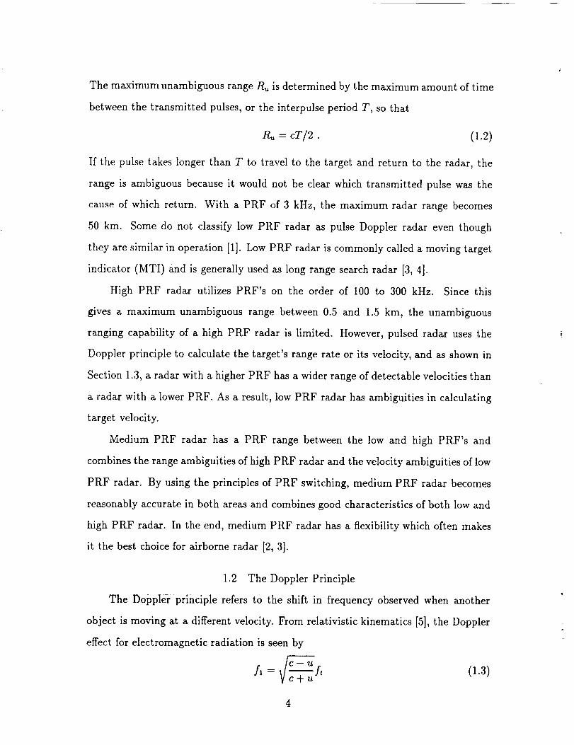
The maximumunambiguousrangeR,_ is determined by the maximum amount of time

between the transmitted pulses, or the interpulse period T, so that

R,_ = cT/2 . (1.2)

If the pulse takes longer than T to travel to the target and return to the radar, the

range is ambiguous because it would not be clear which transmitted pulse was the

cause of which return. With a PRF of 3 kHz, the maximum radar range becomes

50 kin. Some do not classify low PRF radar as pulse Doppler radar even though

they are similar in operation [1]. Low PRF radar is commonly called a moving target

indicator (MTI) and is generally used as long range search radar [3, 4].

High PRF radar utilizes PRF's on the order of 100 to 300 kHz. Since this

gives a maximum unambiguous range between 0.5 and 1.5 km, the unambiguous

ranging capability of a high PRF radar is limited. However, pulsed radar uses the

Doppler principle to calculate the target's range rate or its velocity, and as shown in

Section 1.3, a radar with a higher PRF has a wider range of detectable velocities than

a radar with a lower PRF. As a result, low PRF radar has ambiguities in calculating

target velocity.

Medium PRF radar has a PRF range between the low and high PRF's and

combines the range ambiguities of high PRF radar and the velocity ambiguities of low

PRF radar. By using the principles of PRF switching, medium PRF radar becomes

reasonably accurate in both areas and combines good characteristics of both low and

high PRF radar. In the end, medium PRF radar has a flexibility which often makes

it the best choice for airborne radar [2, 3].

1.2 The Doppler Principle

The Doppler principle refers to the shift in frequency observed when another

object is moving at a different velocity. From relativistic kinematics [5], the Doppler

effect for electromagnetic radiation is seen by

C--/t

A = l/-_-'7__.f, (1.3)vc-ru

where c is the speed of light, ft is the frequency transmitted from the radar source, and

fl is the frequency observed at a target moving relative to the source with velocity u.

The relative velocity u can be interpreted as

u = vi - v_ (1.4)

where vi is the velocity of the target and v_ is the velocity of the source. By recognizing

that the speed of light is much greater than the relative target velocity, the relationship

becomes

fl =f_ ( 1 vi;v_)

The receiver picks up fl shifted again so that

( ),.=,,(1v,_va)_,.c1-2v'-v'+c

(1.5)

(1.6)

where fr is the frequency of the received signal. Since c >> vi - v_, the squared term

becomes negligible and

fr:ft(1-2_) (1.7)

To see the Doppler shift in the frequency domain, take the transmitted pulse

s(t) = A cos(2rftt) (1.8)

where A is the amplitude and the spectrum of s(t) is

S(f) = 1-AeJ(2_rI't+¢) + 1Ae-J(2'_I"+*) (1.9)2

with phase ¢. The return spectrum from a point target is

1 A ,,j(2_r.C_t+_r) 1 A e -j(2_r'frt+4_)s,(f) = _,.,_ + _ _ (1.10)

where fr is given by (1.7) and A, and ¢, are respectively the amplitude and phase of

the return signal. The difference between the returned frequency and the transmitted

frequency is

f,. _ f, = -2 f'(v'- v'_) (1.11)e

which is defined as the Doppler shift.

1.3 Doppler Analysis

In conventional radar notation a positive frequency shift indicates an approaching

target and a negative shift indicates a receding target as shown in (1.11). In order

to keep from having to make the frequency comparison at the transmitted frequency,

the return signal is demodulated down to an intermediate frequency such that the

frequency shift of a return from a stationary object shows up as a frequency shift of

zero. The demodulation of the return signal is accomplished by its multiplication by

a single-sided complex exponential whose frequency is dependent on several factors

involving the source velocity and the geometry of the radar scanning. The return

signal is a discrete sequence of the total return sampled at the PRF rate. The result

of the demodulation is a complex sample for each pulse. By passing the complex

sequence through a low-pass filter, a complex baseband sequence is created. The

resulting complex sequence is called an IQ sequence denoting the fact that the signal

can be divided up into its real and imaginary parts, also called the in-phase and

quadrature-phase components of the complex signal.

Based on Fourier theory for discrete signals, the maximum velocity discernable

with a pulse Doppler radar is limited by the PRF selected. In order to detect a

maximum velocity of +Vm_, the minimum value of PRF is given by

PRFmin = 4Vm.x/._ (1.12)

where _ is the wavelength of the transmitted signal [1]. Since the frequency shift

is best seen in the frequency domain, the Discrete Fourier Transform (DFT) can be

used to obtain the frequency spectrum of the return signal. Because the radar signal

is the complex IQ sequence, the maximum range of the frequency spectrum is the

PRF. Any speeds that are multiples of V,,,_ will cause a Doppler shift that will equal

zero and thus are called blind speeds. Any speeds that are greater than V_ will be

aliased, and their true velocities will be ambiguous.

1.4 Clutter

In any detection system an important factor in the probability of detection is the

signal-to-noise ratio (SNR). In communication systems noise comes from the channel

through which the signal is transmitted and from the system hardware. Since a radar

return is a reflection of transmitted energy, extra noise comes from the reflection of

energy from undesired objects. Such noise is called clutter.

The definition of clutter returns depends on the application of the radar sys-

tem. A ground-based system designed to detect aircraft would receive undesirable

returns from birds and weather. An airborne radar used to detect other aircraft would

consider returns from anything on the ground and any weather as clutter, while an

airborne radar for detecting land vehicles would not consider all ground returns as

clutter.

For weather radar the measurement of windspeed is dependent on returns from

dust particles, rain droplets, and any other small objects which may be blown around

by the wind. Since the individual targets or scatterers are small, the target power

received is low. For an airborne weather radar with the antenna scanning downward or

in the "lookdown" position, the returns from the ground can be much more powerful

than the weather target returns. The concern of this study is lookdown weather radar

scanning in the direction of aircraft travel.

Because Doppler radar measures the frequency shift due to the relative motion

of the reflecting object, the Doppler shift is used to discriminate between moving and

stationary objects. As seen in Section 1.3 the ground clutter is expected to be centered

around zero Doppler [2, 6, 7]. Any moving target within the unambiguous Doppler

capability of the radar will be found displaced from the ground clutter spectrum

center.

For weather radar, clutter can have the effect of biasing the velocity estimate of

wind. A proven method for estimating windspeed is to use the pulse pair method

of estimating the spectral mean of the radar return after filtering out the clutter

7

[6, 7, 8, 9, 10, 11]. Clutter rejection filtering is important since the pulse pair estimate

gives the spectral mean (as shown in Section 4.3.3), and the presence of any clutter

will influence the location of that mean.

All radar systems use some type of a clutter rejection filter to enhance tar-

get detection. Particularly for weather radar where the weather return spectrum is

distributed in the Doppler processing bandwidth, clutter rejection filtering can also

attenuate the power of the low level signal return such that the ability to estimate

windspeed can be affected. A method of estimating windspeed without filtering has

been considered [6]. However, in most cases clutter rejection filtering is successfully

used to aid in the estimation of windspeed [7, 11, 12, 13].

Clutter rejection filtering can be accomplished by various methods. The ground

clutter spectrum is expected to be centered around zero Doppler. One method of

clutter rejection can be accomplished through the implementation of an ideal filter in

the Fourier domain by computing the DFT of the return sequence and then simply

zeroing out the signal power levels at and near zero Doppler. A method that may be

of limited use in airborne radar is clutter map differencing. The principle behind a

clutter map is that the ground objects remain in the same place, but the movement

of the aircraft may make this method difficult to use.

Another popular clutter rejection method is the use of a bandstop filter which

has a narrow notch centered at zero Doppler. The research at NASA in hazardous

windshear detection has made effective use of a second order Butterworth filter with

a notch width of 4-3 m/s [12]. Even though the filter is of low order, its effectiveness

is due to having a transfer function zero at zero frequency.

1.5 Problem Statement

In the implemention of clutter rejection filters, a problem occurs when the clutter

main lobe is shifted away from zero Doppler. Commonly used clutter rejection filters

are designed to be effective only in the neighborhood of zero Doppler. As discussed

8

earlier, in the radar processorthe radar return signal is demodulatedso that zero

Doppler representsa non-movingtarget return along the antennabeam boresight.

However,it is possiblethat the clutter mode can be shifted away from zero after

demodulation,especiallyfor near ranges.For example,a strong target which causes

areturn through anantennasidelobemight dominate theradar return at radar ranges

lessthan the boresight rangeto the ground. An apparent relative velocity would be

indicated eventhough the target is not moving. This clutter mode shifting hasbeen

observedin flight experimentdata, and attempts havebeenmadeto compensatefor

the problem [14]. Investigatedin this work is a method to estimate the shift from

the processedradar return and to employ a clutter rejection filter centeredaround

that shift. Sucha notch without a frequencyreflection which could be centeredat

any desiredfrequencywould necessitatea filter with complexcoefficients.This non-

symmetric notch filter is then comparedto a conventionalsymmetric notch filter on

the basisof its ability to improveclutter rejection.

Chapter 2 explains the processof centering the clutter spectrum by the super-

heterodyneprinciple. Also presentedarevariouscomplicationsto the centeringof the

clutter spectrumand the theory behind the clutter mode shift versusrangein look-

downradar. Chapter 3 coversthe designof filters with complexcoefficientswhich are

derivedby transforming a filter with real coefficients.Chapter4 explainsthe experi-

mentsperformedusingradar data from NASA's windsheardetectionexperimentsand

presentsvariousmethods of calculating the clutter mode shift. Chapter 5 presents

the resultsof testing a complexfiltering schemeon the NASA radar data. Chapter 6

makesconcludingremarksand suggestspossibleavenuesfor further investigation.

9

CHAPTER 2

CENTERING THE DOPPLER SPECTRUM

The complexreturn signal,alsocalled the IQ sequence,is the result of the com-

plex demodulation of the signal. The demodulation of the radar return facilitates its

Doppler analysis by showing an increase in the transmitted frequency as a positive

frequency shift and a decrease in the transmitted frequency as a negative frequency

shift. The radar return has a narrow band of energy determined by the Doppler shift

around the transmitted frequency or radio frequency (RF). Radar receivers commonly

use superheterodyning [1] to get the signal down to an intermediate frequency (IF).

The demodulation of the receiver's IF output is accomplished by the multiplication

of the return by the complex exponential ej_° where w0 is the appropriate frequency

for the centering of the Doppler frequency band.

Superheterodyning refers to the use of two distinct amplification and filtering

stages before demodulation of the signal to baseband. The radar return signal is at

RF and is mixed with a local oscillator signal to create an IF signal. This signal at

IF is then complex demodulated resulting in a two sided spectrum which gives the

entire Doppler range from -PRF/2 to +PRF/2.

2.1 Centering the Radar Return

In order to translate a spectrum to zero Doppler, the radar return is multiplied

by a complex exponential at the frequency of the center of the spectrum. That way an

approaching or a closing target is seen as a positive frequency signal, and a receding

or an opening target returns a signal with a negative frequency.

For a stationary radar, a Doppler shift of zero indicates a stationary target, so

that the demodulation by mixing ft with the return centers the stationary returns

at zero. However, for a moving radar platform, as is the case with airborne radar,

stationary objects havea relativevelocitywith respectto theradar. In order to center

at zero the returns from stationary objects suchasgroundclutter, the demodulation

frequencyis dependenton the velocity of the aircraft.

Extending the discussionin Section1.2,for stationary groundclutter the target

velocity v_ in (1.4) is zero so that the received frequency of stationary ground clutter

in the antenna boresight is given by

fc = ft(1 + 2v:/c) (2.1)

where v_ is the aircraft velocity in the antenna boresight direction. In order for this

frequency to be located at zero Doppler, the frequency for the complex demodulation

of the radar return becomes

fd_,,od = it(1 + 2v./c). (2.2)

Mixing this frequency with the radar return frequency is equivalent to multiplying

the return spectrum by the complex exponential

e-J2rfdem_ t : e-j2_St(l+2v./c) t . (2.3)

Using (1.9) from Section 1.2 as the return spectrum, the result of the multiplication

by (2.3) becomes

1 A ,_j(2_lS,-.fd¢,_o,tltwCr) i A e -j(2r[s'Wfd_m°'tlt+¢r) (2.4)S,Q(f) = 7,.,_ +- 2

or

SIQ(f) = 1A ej(2"[-2s'v'/_lt+¢') + 2AT e-j(2"[2s'-2l'v'/_lt+¢r) (2.5)2 T

By passing SIQ(f) through a low-pass filter, the result is the complex spectrum

SIQ(f) = 1A ej(2"[-2/''/_]'+_") (2.6)2 r

If v_ is the velocity of the ground (which is equal to zero), the result of the demodu-

lation has successfully placed the clutter spectrum at zero frequency.

11

2.2 GeometricConsiderationof Airborne Radar

In (1.4), v_ is defined as the velocity of the source. It should be noted that both

v_ and v_ need to be colinear in order for (2.2) to properly demodulate the radar

return. The measured aircraft velocity is the groundspeed which is the speed of the

aircraft parallel to the ground. When the radar is in lookdown mode, the velocity of

the aircraft relative to a point on the ground is not the groundspeed.

As can be seen in Figure 2.1, the apparent radial velocity of a point on the ground

is equal to V_ = -Vg cos a where Vg is the aircraft groundspeed and a is the angle

between the direction of the aircraft and the line of sight to the point target. The

angle a is a function of both the azimuthal angle ¢0 and the tilt angle of the radar

beam. Notice also that a may differ from the boresight angle a0 due to the antenna

beamwidth. For the airborne radar in consideration here,the narrow beamwidth

keeps this difference negligible. The clutter mode shift has been observed to be a

function of the range to the ground.

The antenna boresight velocity VB can be seen in Figure 2.1 to be related to the

groundspeed Vg by the angle a0 such that

V B = -Vg cos_t_ 0 . (2.7)

The boresight angle ao is related to the azimuth angle ¢o by the antenna tilt angle

¢0 (not shown in Figure 2.1) so that

cos o =cos¢0cos¢0. (2.8)

This equation is used by substituting -VB for v_ in (2.2) to center the clutter spec-

trum.

2.3 Clutter Shifts Due to Sidelobe Returns

In order to determine range information, the radar data is time-gated into range

cells. During the interpulse period, the echo time delay determines the range to

12

Anl;enn(_ boreslght

R

Figure 2.1

-vo

Point t_rge_

Geometry of Lookdown Radar

13

the reflecting target. In the weather radar situation the target is distributed with

many scatterers yielding many echoes. The interpulse period is divided up or gated

into range cells each of which can be characterized by a Doppler spectrum. Figure 2.2

shows a graphical representation of the location of radar range cells along the antenna

boresight. Portions of the main lobe of the antenna beam will intersect the ground

before the boresight does, due to the width of the beam, so that the radar ranges

within the main lobe vary considerably from the boresight range. However, in the

closest range cells, the antenna main lobe does not intersect the ground at all. The

ground clutter returns at slant ranges are from the antenna sidelobes. In the vertical

plane, the antenna sidelobes are returned at a different tilt angle than that of the

main lobe returns. The tilt angle for the sidelobe returns is dependent on the aircraft

altitude and the range to the ground for that particular range cell. The relationship

of the sidelobe tilt ¢side to the range R and the height h is given by

¢side = arcsin h/R . (2.9)

The angle ¢side can be called the sidelobe angle, because it is the tilt angle at which

the sidelobe intersects the ground.

When (2.8) is used in (2.7) to calculate the velocity to be used for the demodu-

lation of the return signal, the boresight velocity Vs becomes

Ys = cos¢0cos¢0 (2.10)

and the demodulating frequency in (2.2) has v_ = -Vs. But according to the pre-

diction of the sidelobe influence in the near ranges, (2.10) should be based on the

sidelobe angle ¢side instead of on ¢0 so that the radial velocity V_ would be

V_ = - Vg cos ¢0 cos(arcsin h / R) . (2.11 )

Figure 2.3 shows how the cosine of the sidelobe angle differs with the cosine of a

constant tilt angle of -3 °. The difference shown in the figure is cos ¢0 - cos ¢side"

14

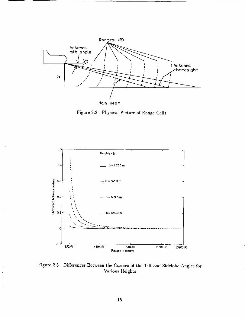
Figure 2.2 PhysicalPicture of RangeCells

0.5

0.4

t_

0.3

8

._ 0.2

_ O.

-0.1

II

I!

III

1I

III

t

I

;\

Heights - h

__ h= 152.5m

.....h = 365.8 m

.-.-.h = 609.6 m

• h = 850.0 m

,• "% %,_

% "% _%

i i I I

852.91 4306.51 7904.01 11501.51

Ranges in meters

13803.91

Figure 2.3 Differences Between the Cosines of the Tilt and Sidelobe Angles for

Various Heights

15

Notice that asthe rangeincreases,the differencebecomessmaller. Also for a lower

aircraft altitude the differenceis not asgreat in the closerangesasit is for a higher

altitude flight. Of course,for a flight that is of high enoughaltitude, the near ranges

would not evenintersectthe ground in the sidelobessothat therewouldbenoground

clutter signal for those rangecells. However,in low flying aircraft such as in final

approachfor landing, the possibility of the clutter shift needsto be considered.

2.4 Other Causesof Clutter Shift

Another problem in centering the clutter spectrum is discrete clutter. Discrete

clutter consists of returns from unwanted moving objects or large, isolated objects on

the ground with a high RCS. In large metropolitan areas a major source of discrete

clutter for airborne radar is an airport terminal and the surrounding city and traffic.

Discrete clutter from large stationary targets can appear away from zero Doppler

and be mistaken for a moving object. The returns from ground traffic and large

buildings could possibly be identified by the location of the objects on the ground

and from other information based on previous knowledge of the surrounding area

and the position of the aircraft. By incorporating this information, an adaptive filter

could be used to eliminate clutter from the return signal. The use of adaptive filtering

based on modeling the discrete clutter is the subject of continuing research [15].

Another possible cause for the clutter shift is the composition of the ground itself.

The amount of power returned in a radar echo depends on the RCS of the scatterer. In

the case of the ground, the RCS is represented as a differential RCS which is averaged

over a unit area. The effective RCS of the ground changes depending on the moisture

of the ground, the amount of vegetation present, and the "flatness" or the shape

of the ground. Such factors could have the effect of spreading the clutter spectrum

making a mean clutter location less useful. The true effect of the composition of the

ground on the clutter spectrum is also a subject of continuing research [31].

16

2.5 Compensating for Clutter Shifts

In order to remove the effects of clutter on signal detection, the notch filter

center frequency should be positioned within the clutter spectrum so that maximum

attenuation of the clutter power can occur. Several approaches for the compensation

of the effects of clutter mode shifting can be taken. One uses the notch rejection filter

centered at zero Doppler. Either the notch width can be adjusted to accommodate for

slight variations in the clutter spectrum mode location, or the clutter spectrum can be

repositioned to be centered at zero Doppler by demodulating the radar return based

on the clutter mode location. Repositioning the clutter spectrum before filtering

would necessitate a reshifting of the spectrum back to its original position after the

clutter rejection filtering has been accomplished to avoid spectrum aliasing which

might bias processing done on the filtered output.

Another method of matching the notch location with the clutter mode location

would be to use a notch filter with a movable notch. Such a filter would need to

have complex coefficients in order to have a response that is not symmetric about

zero Doppler. The design of such a filter is discussed in Chapter 3. The advantage

of using a complex filter is that the clutter mode could be filtered without having to

shift the clutter spectrum. The main computational requirement is the estimation of

the clutter mode location which is also a requirement for the clutter spectrum shifting

method. In the analysis to follow the use of a movable notch clutter rejection filter

will be considered.

17

CHAPTER 3

A FILTER WITH COMPLEX COEFFICIENTS

Digital filter designis a basic knowledgenecessaryin digital signal processing.

Radar processorsuse digital signal processingbecauseit allows sophisticated pro-

cessingof the radar return signal for automatic detection and tracking. The nature

of pulse Doppler radar automatically createsa digital sequencewhich is the return

signal sampledat the PRF. The demodulation of the return createsthe IQ sequence

which is a complexvaluefor eachpulsetransmitted. An important part in processing

the IQ sequenceis the useof digital filters for clutter rejection filtering.

3.1 Digital Filters

Oneimportant method of designingdigital filters is basedon the transformation

of anappropriate analogfilter. Textbooksdiscussthe methodand theory of designing

an analogfilter from a prototype and convertingit into a digital filter [16, 17]. Signal

processingsoftware packagesinclude filter design programswhich can be used to

designIIR and FIR filters by a numberof different methods.

A commonfactor of thesepopular filter designmethods is that the resulting

digital filters all havereal coefficients.Of course,real arithmetic is lessof a computa-

tional load than complexarithmetic. However,a filter with real coefficientsis limited

to having a frequencyresponsethat is symmetricabout zerofrequency.

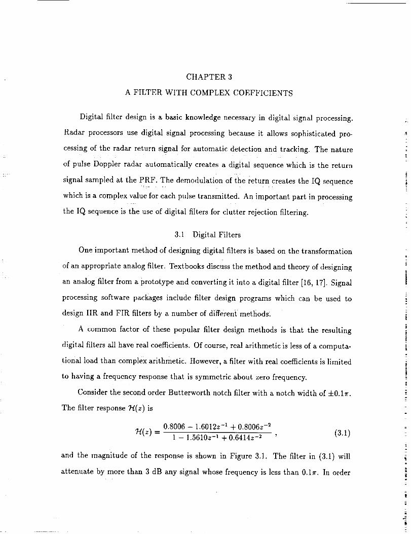
Considerthe secondorder Butterworth notch filter with a notchwidth of +0.17r.

The filter response 7"((z) is

0.8006 - 1.6012z -1 + 0.8006z -2

_-/(z) = 1 - 1.5610z -I + 0.6414z -2

and the magnitude of the response is shown in Figure 3.1.

(3.1)

The filter in (3.1) will

attenuate by more than 3 dB any signal whose frequency is less than 0.1r. In order

zqt

E_i

it

i

-20

-6O

-80

-I00-I -018 -0'.6 -OJ.4 -012 0 012 014 016 018

freqpi

Figure 3.1 Real Filter with Notch at Zero

19

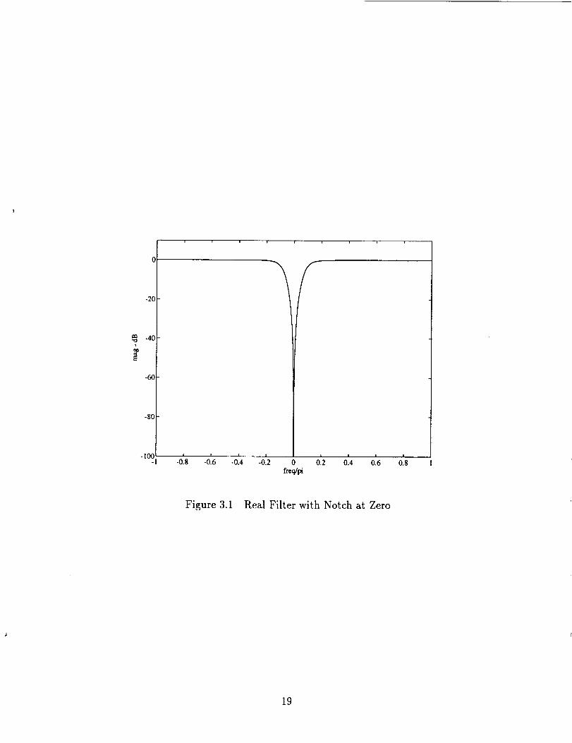
to attenuate by at least 3 dB a signal at 0.37r, either the notch could be widened, which

would filter out every signal less than 0.3r, or the notch could be moved. Redesigning

a Butterworth filter with an equivalent notch located at 0.3r while retaining real

coefficients results in the transfer function

0.6389 - 1.5105z -1 + 2.1706z -2 - 1.5105 z-3 + 0.6389z-4(3.2)

7-[t(z) = 1 - 1.8575z -I + 2.0357z -2 - 1.1635z -3 + 0 -4128z-4

The filter has now become a fourth order filter, and as seen in the magnitude of the

response of 7-[t(z) in Figure 3.2, the filter not only stops a signal at 0.3rr but also any

signal at -0.37r. The only way to have a notch filter which would attenuate a positive

frequency without any attenuation at the negative of that frequency is to design a

filter with complex coefficients.

3.2 A Filter with a Shifted Frequency Response

Because conventional filter design theory cannot directly solve for complex filter

coefficients, the complex filter is derived by the transformation of a real filter. A sim-

ple transformation is a frequency shifting transformation which centers the frequency

response away from zero [18]. The frequency shifting transformation is based on the

representation of a bandpass signal as a low-pass envelope times a complex exponen-

tial. For the bandpass signal z(t) centered at _vc, its envelope x(t) is multiplied by

exp[jwct] so that

z(t) = x(t) j o' . (3.3)

By taking the Fourier transform of z(t), the bandpass signal becomes

= (3.4)

which is the envelope signal shifted to the frequency w_.

Another way to represent a complex signal is to recognize it as a real signal

with the negative frequency components zeroed out. The creation of such a signal is

accomplished by letting the real part be the original real signal and by having the

2O

-2O

-40

-6¢

-8£

-10o-1 -o'._ _ 0'.3

freo,/_

Figure 3.2 Real Filter with Notch Shifted to 0.3r

21

imaginary part equal the Hilbert transform of the real signal. The Hilbert transform

of a real signal x(t) is

1k(t) = x(t) • --. (3.5)

7rt

Basically the transformation results in a -90 ° phase shift of the original. For example,

the signal

has the Hilbert transform

x(t) = A cos(co0t + ¢) (3.6)

k(t) = Asin(coot + ¢). (3.7)

A complex signal whose imaginary part is the Hilbert transform of its real part isZ

called an analytic signal, and it has half the bandwidth of the original real signal.

From the example above, the analytic signal would be

x(t) + jk(t) = A[cos(wot + ¢) + jsin(wot + ¢)] (3.8)

which is equal to the complex exponential Ae j(_°t+¢).

To create a complex filter centered at coc5¢0 the filter impulse response is multi-

plied by exp[jcoct] as shown above. This equates to replacing s by sa = s -jcoc in the

transfer function H(s) of the filter with real coefficients. Realizing that the s-plane

is related to the z-plane by the relationship

z=e r , (3.9)

we can determine that z wql be replaced by

Z 1 : eSl T = e(s-jw_) T = e-JwcTz (3.1o)

in 7-f(z). By letting

3' = e-J_cT , (3.11)

we see that (3.10) becomes z replaced by zl = 7z.

22

Since each pole or zero is described by

(z - a) =0, (3.12)

it follows that replacing z with Zl results in the pole or zero becoming

(z- _-'a) = 0. (3.13)

In other words the shifted pole is the original pole rotated by weT radians. The filter

response can be written as the ratio of polynomials

ao + alz + ... + a,,z'*

"H(z) = bo + blz + "'" + bmz m '(3.14)

and the shifted filter becomes

aos + alsz + • • • • ansZ n

7-l,(z) = bos + bisz +"" + bmsz m(3.15)

where ats and bt, are the complex coefficients and are derived by

ate, = 71at and bt, = 7tbt. (3.16)

For a transfer function in terms of polynomials in the delay operator z -1, the complex

coefficients become

cts = 7-tct and dts = 7-tdt , (3.17)

and

COs "-I- ClsZ -1 "l'- "'" _ Cns Z-n

_s(z) = do, + dx,z-' + "'" + dmsz -_(3.18)

To see an example of this transformation, note the filter response in (3.1) with a

shift to 0.37r. Using (3.10) the filter response becomes

7-/c(z) = 0.8006 - (0.9412 + jl.2954)z-' - (0.2474 - j0.7614)z -2 (3.19)1 - (0.9175 + jl.2629)z -1 - (0.1982 - j0.6100)z -2 '

and the magnitude response does not have the negative frequency reflection as shown

in Figure 3.3. Also notice that the order of the filter is preserved.

23

-20:

-40t

-5O

-gO

-100-1 o13 •- 0

_eq/_0.3

Figure 3.3 Complex Filter with Notch at 0.3_

24

3.3 A Filter with an Asymmetric FrequencyResponse

Another transformation which shifts the center frequencyof the filter response

hasbeen describedin the literature [19], but it yields a magnitude responsewhich

is asymmetricalabout the centerfrequency.This transformation is accomplishedby

usingthe bilinear complexfunction

s = sl - ja (3.20)1 -4-jasl

as a frequency transformation function. The most general form of the transformation

is given by

8 = (mS1-- jX) - ja (3.21)1 + ja(msl -- jx)

where the parameters m, x, and a(lal < 1) are parameters that determine the band-

width, the center frequency, and the asymmetrical characteristic of the desired com-

plex filter. By using the bilinear transformation to change analog to digital, the filter

transformation becomes

act a ct

z -1 + zl 1 (3.22)b 1 + az 1

where

a= l + ax - m - j(am + x + a) (3.23)1 + ax + m + j(am - x - a)

and

b = 1 + ax + m + j(am - x - a) . (3.24)

The parameters m, z, and a are solved for by equations involving the desired shape

of the resultant filter [19].

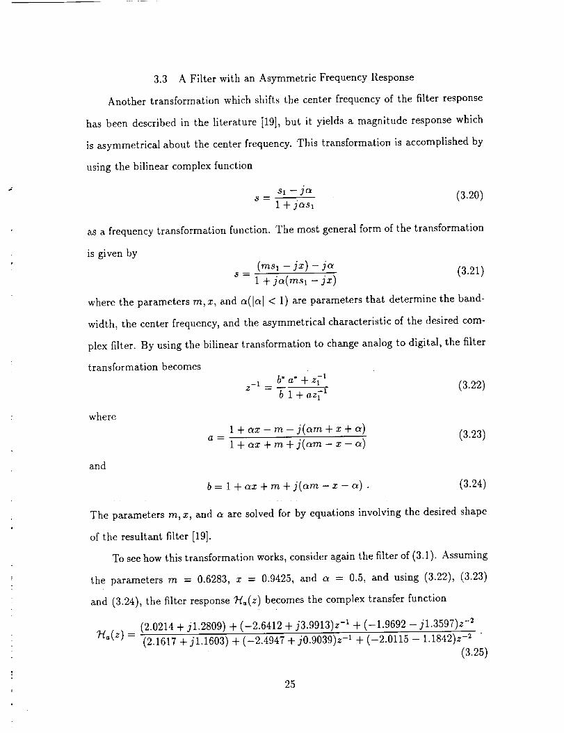
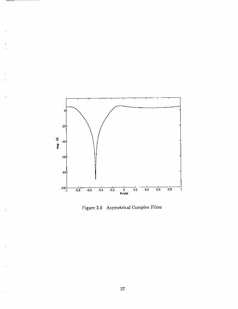
To see how this transformation works, consider again the filter of (3.1). Assuming

the parameters m = 0.6283, z = 0.9425, and a = 0.5, and using (3.22), (3.23)

and (3.24), the filter response 7-/,(z) becomes the complex transfer function

(2.0214 + jl.2809) + (-2.6412 + j3.9913)z -1 + (-1.9692 - j1.3597)z -2

7-/_(z) = (2.1617 + ji.1603) + (-2.4947 + j0.9039)z-' + (-2.0115 - 1.1842)z -2

(3.25)

25

The asymmetrical responsecan be seenin Figure 3.4. This transformation is a bit

more involved than the frequencyshifting transformation, yet it allows for the flex-

ibility of a filter whoseresponseis truly asymmetrical. Other asymmetrical trans-

formations can be created by variations on the original transformation such as the

reciprocal of (3.20).

3.4 Implementingthe ComplexFilter

Whena filter with real coefficientsis usedon a complexor analytic signal,every

operation is performedtwice. Eachdelay,addition, and multiplication needsto occur

for both the real and the imaginary parts of eachcomplexsample. For eachsample

the real and imaginary parts needto be kept separate.

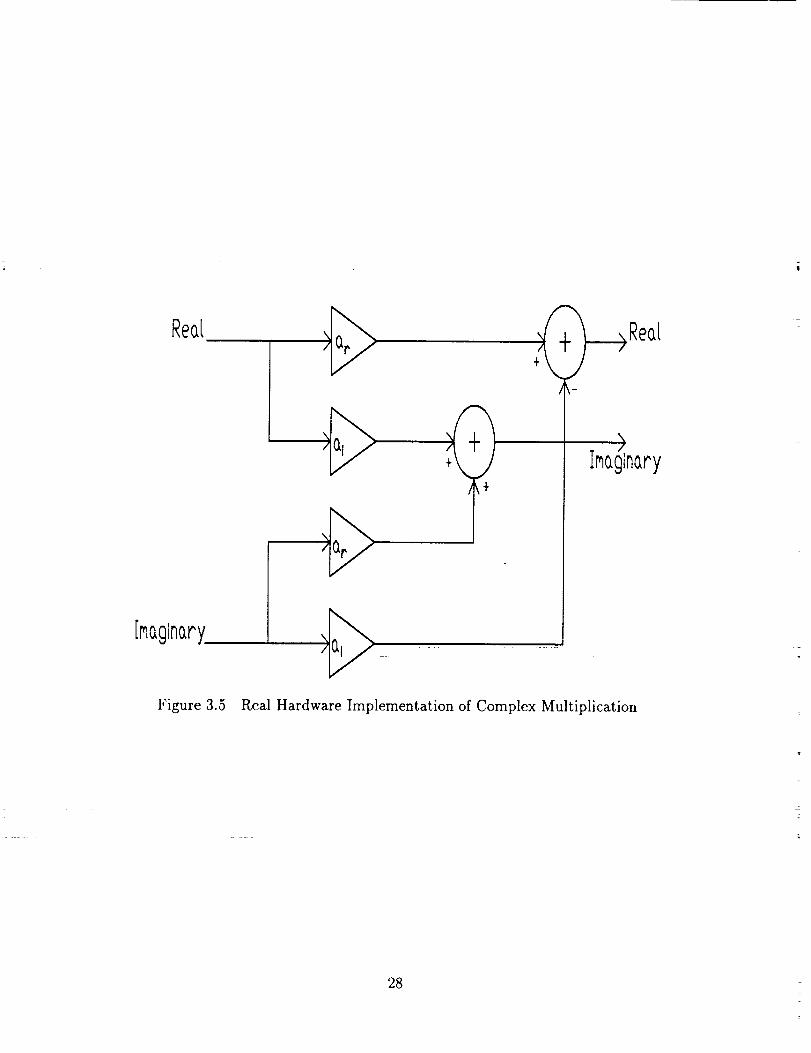
For a filter with complexcoefficients,the delaysand addersremainthe sameas

above. The only differenceis in multiplication becauseof the multiplication of two

complexnumbers. The multiplication of the complexsampleX(n) = zr(n) + jzi(n)

by the complex coefficient A = aT + jai becomes

AX(n) = [arr(n) - aix(n)] + j[air(n) + a_x(n)] . (3.26)

The increase in the number of operations to be performed is the price that is paid for

having to use complex arithmetic.

Since complex arithmetic is easily expressed in terms of real arithmetic, real

hardware can be used to implement a complex filter [20]. Figure 3.5 shows the real

hardware implementation of a complex multiplication. For the other operations, the

delays and additions of the real and imaginary parts are done in parallel.

once the Complex components have been establishedl the complex filter is im-

plemented in the same manner as a real filter. Any of the real filter realizations can

be applied to a complex filter, allowing for the realization of the filter in the most

desirable configuration. A parallel realization of the complex sections of a filter has

a number of good properties since it is a minimum norm structure [20]. A minimum

26

-2O

-4O

-6O

-80

-1o_-1 -01.8 -01.6 -0_.4 -01.2 ; 012 0'.4 016 018

freq/pi

Figure 3.4 Asymetrical Complex Filter

27

Rear

[maglnary

Figure 3.5

)÷

Real Hardware Implementation of Complex Multiplication

>IMaglnary

28

norm structure is a filter in which the norm of its system matrix has been minimized.

In the analysis presented in Chapter 5, the filters are implemented as transposed

direct-form II.

It is interesting to notice how shifting the center frequency of the filter affects

the notch depth. The original Butterworth filter of (3.1) has a magnitude response of

zero at zero frequency. Theoretically, the frequency shifted complex coefficient filter

as designed by using (3.10) should also have a magnitude response of zero at the notch

location. It turns out that due to coefficient quantization there is a small difference

between the actual magnitude response and zero. A filter realized such that it is a

minimum norm structure has been shown to have the characteristic of low roundoff

noise [21] which could decrease the difference between the actual magnitude response

and the desired response of zero. However, the difference is already minute enough

that it can be considered to be zero. The ability of the complex coefficient filter to

zero out clutter power at the notch location is a desirable characteristic for clutter

rejection filtering.

29

CtIAPTER 4

TESTING A MOVABLE NOTCH FILTER

It is quite obvious that a filter with a movable notch could be used to compensate

for clutter mode shifts that may occur with airborne radar. To test the use of the

movable notch filter, actual radar data are used. The radar data comes from NASA's

research in evaluating airborne radar as a means of detecting hazardous weather [13]

and is from a forward looking radar operating at low altitudes with a tilt angle of

-1 to -3 degrees. Four different approaches are considered for adapting the clutter

notch position.

4.1 NASA Research on Itazardous Windshear Detection

Low altitude windshear has been recognized as a potential hazard for aircraft

taking off for a flight or approaching for a landing [22]. Since the low-level microburst

has been identified as the cause for many plane crashes in tile terminal area, NASA

has taken up a study on remotely sensing the hazardous weather. The detection of

hazardous windshear with airborne pulse Doppler radar has been the topic of many

previous papers [6, 7, 10, l 1], and the development of a working low-level windshear

alert system is now being accomplished at private avionics companies, e. g. [23].

An important part of detecting a hazardous windshear is the definition of what

is meant by hazardous. This has led to a definition of the hazard factor based on the

horizontal and vertical windspeeds and on the aircraft velocity [24]. Using aircraft

accelerometer data to estimate this hazard factor, a severe windshear can be identified

with high probability [2.5]. Although the timing of such an in situ identification may"

not be sufficient for the avoidance of potential catastrophe, such information is useful

in tile validation of a remotely sensing system.

The investigation into remotely sensing systems has led to several possibilities.

Currently in use are the next generation weather radar (NEXRAD) [26] and the

ground basedTerminal Doppler WeatherRadar (TDWR) [27, 28]. NEXRAD instal-

lations form the backboneof the U.S.aviation weathersystem[29] and can provide

detection of low--altitude windshearevents. TDWR has proven to be an effective

method for detecting win&hear and hasservedas a testing ground for hazard algo-

rithms for airborne systems. A telemetry link from the TDWR to the cockpit can

providedirect information to the pilot concerningdangerouslocations in the terminal

area [30].

The possibleforward looking airborne sensorsinclude a pulse Doppler radar,

LIDAR (Light Detection and Ranging), and FLIR (Forward Looking Infrared Ra-

diometer). Eachsystem'ssensingcapabilities can be verified by the in situ algorithm

and corrolated with data from the TDWR. Future operational windshear detecting

systems will likely consist of an integrated combination of various systems.

NASA Langley Research Center has conducted flight tests during 1991 and I992

including flights at tile airports of Orlando and Denver during the potential storm

season in the summer. Each flight took place in the near terminal area and included

landing approaches and take offs [13]. Many clutter-only flights were performed in

order to get a good picture of the ground clutter and the discrete clutter experienced

in the terminal area. Weather flights were performed when a storm system was sensed

and determined safe enough to fly through. By flying through a storm, the crew could

determine the effectiveness of a remote sensing system to estimate the hazard factor

as compared to the in situ measurements.

4.2 The Radar Data

The radar data used for this paper come from NASA's Wind Shear Flight Experi-

ments. The airborne radar used in these experiments as a remote sensor for hazardous

windshear operates in X-band at 9.3 GItz. The radar system can operate at several

user-selected PRF's with much of the data collected using a PRF of 3755 Hz with a

pulse width of 0.96 #s. The Doppler range at this PRF is -t-30 m/s with a resolution

31

of 1 m/s. Data wererecordedover a rangeof 14km to be able to give an advance

warning of about 15 to 40 seconds[12].Tile azimuth scanof up to 4-30 ° guarantees

that the entire area in the flight path can be scanned for a possible hazard.

The data used in this analysis consist of records of complex samples from 96

consecutive pulse returns collated according to the radar range. The radar ranges vary

from 850 m to 13.8 km including range cells 6 to 96 with each range cell corresponding

to the range resolution of the radar, 144 m. Each record of data is indexed according

to the antenna scan azimuth angle which varies in 0.5 degree increments over the

scan. The data are samples of the receiver IF output and include an AGC (automatic

gain control) value within each range cell to extend the effective dynamic range of

the A/D converter. The data are "raw" in that there is no pre-processing performed

on it.

4.3 Implementing the Movable Notch Filter

The complex filter design method considered here and implemented is the method

explained in Section 3.2 and defined by (a.10). The real valued filter which has been

most often used in analysis work at NASA is a second order Butterworth high pass

filter with a notch width of +3 m/s or +0.1_. It is readily apparent that shifting the

filter notch is a very simple procedure. The main problem is defining where to shift

the filter notch.

4.3.1 Predicting the Clutter Mode Shift

For the NASA win&hear radar the centering velocity used is given in (2.10). The

difference due to the sidelobe angle can be calculated using the altitude information

of the aircraft and the range distance of the particular range bin. From (2.11) we get

the true radial velocity of the clutter scatterer so that the received frequency of the

clutter is given by (1.7) to be

f_ = f_ 1 + --cos_bocos(arcsin h/l_) (4.1)¢

a2

Since the frequency used in (2.2) uses the boresight velocity of (2.10) the demodulating

frequency becomes

fde,_od = ft 1 +--cos¢0cos¢0 (4.2)C

In the frequency mixing of (2.4) the resulting observed Doppler shift becomes

f_ fd_moa ft 2Vg- = cos ¢o [cos(arcsin[h/R]) - cos ¢0] (4.3)C

which ought to be the amount of the clutter shift away from zero. By using this

algorithm to predict the shift of the clutter away from zero, the complex filter should

be centered at the center of the clutter spectrum.

The accuracy of the prediction of the clutter shift is subject to several variables.

First of all, in the closer range cells the angle at which the ground is intersected is out

of the main lobe of the radar beam. The resulting spectrum is spread in frequency,

usually without a main clutter mode. Another possibility is that second time around

returns appearing in the main lobe of the antenna may be of significant relative mag-

nitude to bias the returns in the closer range cells. Second time around returns refer

to returns which come from beyond the radar's maximum unambiguous range. Stud-

ies have indicated that some second time around returns appear in the closer range

bins and that they are less of a problem as the antenna tilt angle increases [31]. The

accuracy of the shift predictor is also susceptible to variations in the measurements

of the aircraft groundspeed and altitude. A very important point to notice is that

a clutter mode shift in the close ranges can occur due to factors other than just the

sidelobe returns, which would make the prediction of the shift inaccurate.

4.3.2 The Peak Finder

A possible method for estimating the center frequency shift based on the return

data is to use a peak finder. The assumption is that the dominant spectral power

mode from ground clutter is located in frequency by the spectral peak and that this is

the best position for a clutter rejection filter. In order to implement the peak finder,

33

a radar signalfrequencyspectrumestimate is usedto identify the frequencylocation

with the largest magnitude.

One problem with the peak finder method of calculating the center frequency

shift is that it may bebiasedby very largereturns from discreteclutter suchasthat

associatedwith moving targets. To discriminate against discrete clutter, a system

would need either a logic program that dismissesa solitary peak as discrete or a

limiting program that only calculatesa frequencyshift in the closerrangecellswhere

the sidelobeshift is predicted to bemoreprevalent.

4.3.3 The Pulse Pair Estimator

In a clutter-only situation the location of the spectral meancan be calculated

using the pulse pair algorithm. The pulse pair method has been proven to be a

desirable way to estimate the mean velocity for a weather return [8] and can be

expectedto give a reliableestimateof the spectralmeanwhenevera dominant mode

is present. If there is nothing but clutter present in the return, a pulse pair mean

estimateshouldbea good indicator of the clutter mode. The pulsepair estimator is

a problemfor practical usesinceit is not a good spectral modelocation identifier if

more than onemodeis present.A discussionof the pulsepair algorithm hasappeared

in many workson the detectionof hazardouswindshear [6, 7, 11, 12].

The pulse pair estimateof the spectral meanusesthe autocorrelation function

estimateof the complexdata sequenceat the first lag. For a complexsequencex with

N data points, the autocorrelation function estimate at the first lag is

1 N-2

/_(1) = _ _ x(j + 1)x*(j) . (4.4)j=0

The pulse pair mean Doppler velocity estimate follows as

vpp = 47rTarg[R(1)] (4.5)

where )_ is the radar wavelength and T is the interpulse period or 1/PRF. The pulse

pair estimator can also be calculated using a power spectrum estimate of the complex

sequence x [8].

34

4.3.4 AutoregressiveModeling

A moresophisticatedmethod of estimating the spectral modelocation is based

upon the useof the extendedProny method, which usesa linear modelingof the

clutter return. Keelusesthe autoregressive(AR) modelto modelthe clutter spectrum

and thus to designa clutter rejection filter [11]. Earlier work had suggestedthat the

AR model is a useful tool in modeling the ground clutter returns [32]. In Keel's

study, a 10th order AR model was used to estimate the clutter spectrum, and a

clutter rejection filter wasdesignedby using the inverseof the AR model asan FIR

filter. Although the methodspresentedby Keel areattractive from a theoreticalview,

the needfor a true clutter-only return to create the model and the computational

load of AR modelingpresentimplementationproblems.

Kunkel [6] employsa secondorder AR model in an extendedProny algorithm

to identify clutter and weathermodes.By using his modal analysisprinciples, it is

possibleto identify the clutter mode as the location of the clutter spectrum shift.

This implementation is similar to the pulse pair estimate, but it is superior in that

it accounts for more than just one mode thus enabling the processor to characterize

both the weather location and the clutter location when they both appear. At low

return power levels the mode estimates tend to fluctuate randomly near the maximum

Doppler shift value. A simple power level threshold can be effective in identifying

erroneous large shifts.

By using the Levinson-Durbin algorithm to calculate the second order AR coef-

ficients ax and a2, the extended Prony approach solves the characteristic polynomial

#2 + al/_ + a2 (4.6)

for the values of #x and #2 which determine the frequency estimates. The frequency

estimates determine the weather and clutter velocities in a manner similar to the

pulse pair velocity described above. The velocities are calculated by

v, = -4roT arg(#,) . (4.7)

35

Kunkel defines the clutter velocity as the velocity whose absolute value is closer to zero

of the two velocities [6]. The Levinson-Durbin algorithm is described in Appendix A.

4.4 Testing the Shift Estimators

By using the various shift estimators to locate a notch to filter the clutter return,

the effectiveness of each estimator to calculate the clutter spectral shift can be de-

termined. If the signal used is clutter-only, the resulting signal power after filtering

can be examined. The shift estimator which is most effective would reject the most

clutter and thus would result in the lowest power after filtering.

Another area in which the shift estimators should be compared is in the amount

of computation necessary to implement each estimator. Although the peak finder

seems simple enough, a DFT computation is required for each range cell. Even with

an efficient FFT algorithm, it is still time consuming. The pulse pair estimator uses

an autocorrelation estimate which is much more efficient than the FFT. For low order

models the modal analysis methods involve simple correlation estimates from the data

and can be efficiently implemented. The mode prediction is not data dependent and

is thus the simplest of all computationally.

The next chapter details the results of experiments for this work. First of all

the shift estimators are compared in their ability to estimate the clutter mode shift.

Then the power levels after filtering are compared to see which estimator is the most

effective. More importantly the results are used to evaluate the effectiveness of a

movable notch filter with complex coefficients as compared to the more conventional

fixed notch filter with real coefficients.

36

CHAPTER 5

RESULTS

In this chapter the predicted clutter shift (as discussed in Section 4.3.1) will

be compared to the data dependent clutter shift estimators presented. A shift in

the clutter of the closer range cells can be observed by looking at frequency plots

of the clutter run data. The data set used for analysis is clutter-only recorded over

Denver, Colorado, on 9 July, 1991. The data consist of 257 frames covering an entire

antenna scan from 0 to -30 ° to +300 and back to 0 at 0.5 ° increments. This scan

was randomly selected and consists of frames 200 to 456. Data at scan angles +5 °

(Frame 200), -30 ° (Frame 270), and -6.5 ° (Frame 320) were chosen to be displayed

in this chapter, and Appendix B consists of a complete listing of range cell frequency

plots for Frame 270. The tilt angle was a constant -3 °. The variation in the aircraft

height and velocity was small since the frames were taken so close to each other, and

it turns out that this variation had little effect on the data.

Each spectral estimate is plotted in the weather radar convention of power versus

windspeed. The windspeed is calculated from the original Doppler shift equation

given in (1.11). For a target moving toward the radar, the relative velocity u is less

than zero so that the Doppler shift fa is greater than zero. Rewriting (1.11) with

u = vi - v_, and fd = fr - ft yields

= , (5.1)¢

which shows the opposite sign relationship between the velocity and the Doppler shift.

In the case of weather radar, the centering algorithm removes the aircraft velocity so

that the direction of the wind determines the sign of the relative velocity u, and the

Doppler frequency shift is as given above. From (1.12) and the radar parameters, the

maximum Doppler velocity is +30 m/s.

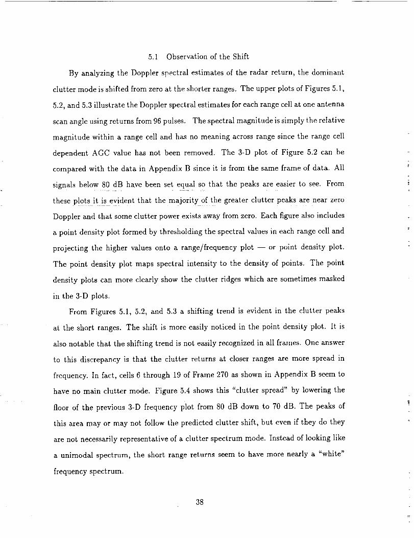
5.1 Observation of the Shift

By analyzing the Doppler spectral estimates of the radar return, the dominant

clutter mode is shifted from zero at the shorter ranges. The upper plots of Figures 5.1,

5.2, and 5.3 illustrate the Doppler spectral estimates for each range cell at one antenna

scan angle using returns from 96 pulses. The spectral magnitude is simply the relative

magnitude within a range cell and has no meaning across range since the range cell

dependent AGC value has not been removed. The 3-D plot of Figure 5.2 can be

compared with the data in Appendix B since it is from the same frame of data. All

signals below 80 dB ha, ve been set equal so that the peaks are easier to see. From=

these plots it is evident that the majority of the greater clutter peaks are near zero

Doppler and that some clutter power exists away from zero. Each figure also includes

a point density plot formed by thresholding the spectral values in each range cell and

projecting the higher values onto a range/frequency plot -- or point density plot.

The point density plot maps spectral intensity to the density of points. The point

density plots can more clearly show the clutter ridges which are sometimes masked

in the 3-D plots.

From Figures 5.1, 5.2, and 5.3 a shifting trend is evident in the clutter peaks

at the short ranges. The shift is more easily noticed in the point density plot. It is

also notable that the shifting trend is not easily recognized in all frames. One answer

to this discrepancy is that the clutter returns at closer ranges are more spread in

frequency. In fact, cells 6 through 19 of Frame 270 as shown in Appendix B seem to

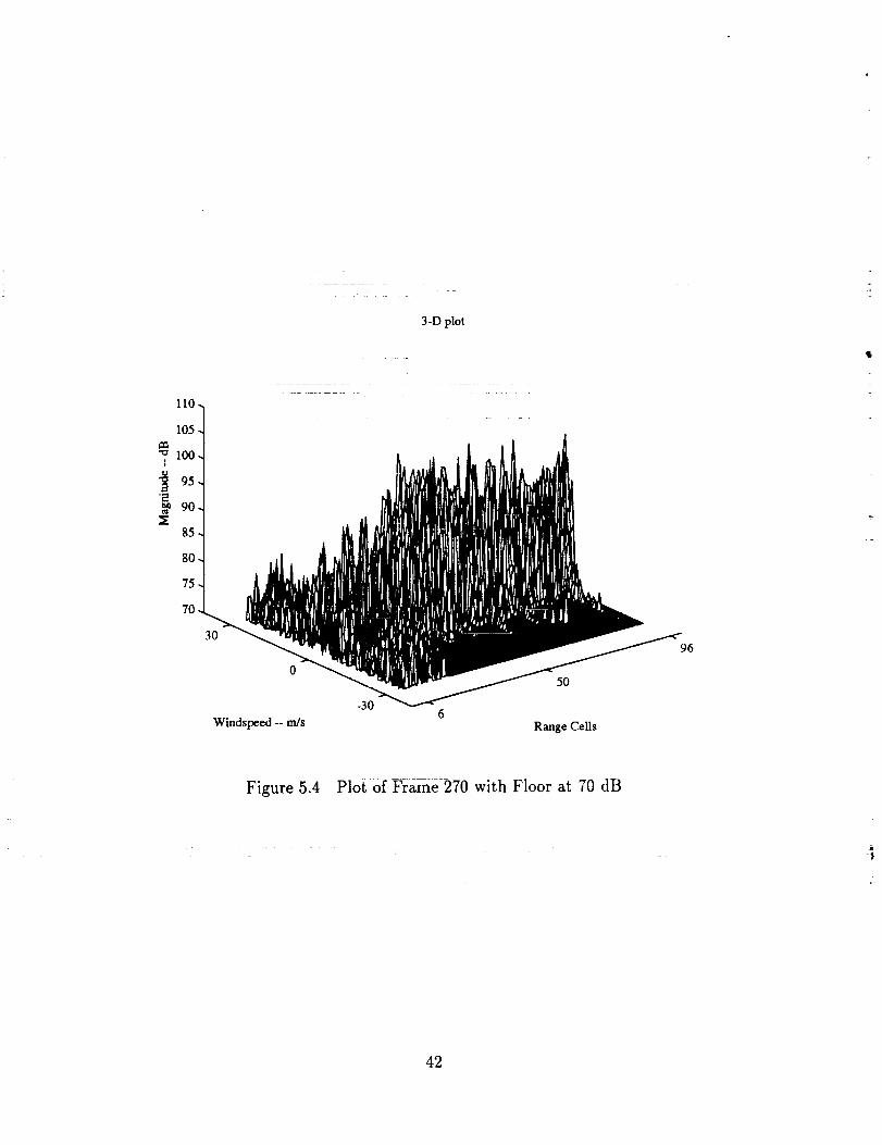
have no main clutter mode. Figure 5.4 shows this "clutter spread" by lowering the

floor of the previous 3-D frequency plot from 80 dB down to 70 dB. The peaks of

this area may or may not follow the predicted clutter shift, but even if they do they

are not necessarily representative of a clutter spectrum mode. Instead of looking like

a unimodal spectrum, the short range returns seem to have more nearly a "white"

frequency spectrum.

h

38

3-Dplot

II

_o"O 100-

90

80

30

0

Windspeed.-m/s

96_

80

60

_0

20

6

-30|

-20

PointDensityPlot

1 I I

-10 0 10

Windspeed- m/s

50

RangeCells

i

20

96

J

30

Figure 5.1 Plots of Frame 200

39

3-Dplot

80

30

0

Windspeed-m/s

96

80

60

O

20

6 _ _..... !

-30 -20I

-10

PointDensityPlot

I

0

Windspeed--m/s

50

RangeCells

I I

10 20

96

!

30

Figure 5.2 Plots of Frame 270

40

3-Dplot

_9

._

110

I00

90

80

96

80_

600

4o

20

-30

30

0

Windspeed--m/s

I

-20

PointDensityPlot

I i I

-10 0 10

Windspeed--m/s

50

RangeCells

!

20

96

i

30

Figure 5.3 Plots of Frame 320

41

110.

105

_ looI

95N 90

85

80

75

70

3-D plot

30

50

-306

Windspeed --m/s Range Cells

96

'lg

Figure 5.4 Plot Of Frame 270 with Floor at 70 dB

42

5.2 Comparison of the Shift Estimators

As shown in Section 4.3, there exist several methods (the peak finder, the pulse

pair estimator, and the extended Prony method) of estimating the frequency shift of

the clutter spectrum mode and these estimates can be used to compare the observed

clutter mode with the clutter shift predictor given in (4.3). The clutter shift predictor

varies with the aircraft height, velocity, and the antenna azimuth angle, and since for

this particular flight the height and velocity were relatively constant, the variation

depends primarily on the azimuth angle. Even so, the predicted clutter mode shift

does not vary significantly for the frames examined.

Figure 5.5 shows the comparison of the peak finder with the frequency shift

predictor. The trend of the peak finder does follow the shift predictor, but as can be

seen in the comparison on Frame 270, the variance can be large. These variations are

mostly due to the Doppler frequency spectral spread and lack of a dominant mode

in the close range cell returns as shown in Appendix B. Since the clutter spectra

in the closer ranges of Frame 270 are more spread in frequency, characterizing each

spectrum as unimodal at a single frequency based on the greatest power may not be

useful due to the lack of a dominant clutter mode.

In Figure 5.5 note the peak finder's "spike" in Frame 200 at range cell 82 which

may be due to discrete clutter. As mentioned before, discrete clutter can show up

as a high energy return away from zero Doppler. Here again, the selection of that

peak as the dominant clutter spectral mode is not representative of the true clutter

spectrum. By examining the range cell spectra of Frame 270 in Appendix B, the

separation of the dominant clutter spectrum and discrete clutter can be easily seen.

Next the pulse pair algorithm as a clutter mean estimator is compared with the

frequency shift predictor. In Figure 5.6, the pulse pair estimates of the mean clutter

frequency exhibit similar variations as were noted in Figure 5.5 with the peak finder

results. Since the pulse pair deviations are not as large as those for the peak finder,

one can deduce that there must be more than one spectral "peak" in the cell spectrum

43

30

!

I

"t:l¢) 0

_:-3C

30

I!

o

"0

-30

30

II

-3o

Frame200

_ peakfinder... shiftpredict

i | | , | i |

6 15 30 45 60 75 96

RangeCells

Frame270

_ peakfinder... shiftpredict

l i . | J | ,,, i I

6 15 30 45 60 75 96

RangeCelts

Frame320

v

__ peakfinder,,, shiftpredict

i i i | i | |

6 15 30 45 60 75 96

RangeCells

Figure 5.5 Comparison of the Peak Finder with the Shift Predictor

44

_h

i!

"t:loo

'0

_, 30̧

!!

o 0t/l

-30

30

II

o 0

-30

30

-30

Frame200

|

6 15

• o .... ., . ......

pulsepairmean... shiftpredict

|

30 45 60 75 96RangeCells

Frame270

_ pulsepairmean... shiftpredict

6 15 30 45 60 75

RangeCells

Frame320

96

_ pulsepairmean... shiftpredict

||

6 15 30 45 60 75 96

RangeCells

Figure 5.6 Comparison of the Pulse Pair Algorithm with the Shift Predictor

45

influencing the spectral mean since a single spectral mode would tend to dominate

the mean estimate. The multiple peaks can be seen by looking at the spectrum of

each range cell as mentioned above.

As it has been shown, the pulse pair algorithm gives a mean over the entire

range cell spectrum [6]. Thus a pulse pair estimate for a cell in which discrete clutter

is also present would not accurately represent the spectrum of either the dominant

clutter near the aircraft groundspeed or the discrete clutter which may be displaced

in Doppler. Also in cases where weather returns are present, the pulse pair mean

may not accurately estimate the clutter shift. Results using the pulse pair mean are

presented here to validate the peak finder.

The extended Prony analysis technique of Section 4.3.4 for estimating the main

lobe clutter frequency shift is compared with the frequency shift predictor in Fig-

ure 5.7. The extended Prony analysis can also be called the clutter mode identifier

since it identifies the "mode" which should represent the clutter spectrum and dif-

ferentiates it from a weather mode. This second order clutter mode identifier can

recognize two distinct modes distinguishing it from the pulse pair algorithm.

As can be seen, the clutter mode technique is similar to the peak finder and

the pulse pair algorithm at following the frequency shift predictor. Based on stud-

ies involving modal analysis [6], the clutter mode technique probably has the most

credibility for providing a good frequency shift estimate. Once again the effect of

discrete clutter must be considered. It would appear that the clutter mode technique

should be able to identify the main clutter in the presence of a discrete clutter mode

although the presence of a weather mode may reduce its effectiveness. A higher order

autoregressive model could be used to model the clutter spectrum which in turn could

be used to identify not only the main ground clutter location but also any number

of discrete clutter locations [11]. Of course the price for a better clutter identifier

through a higher order AR model is the increased computational intensity required

to solve for the AR coefficients.

i

46

c/l

30II

oo 0t_

-30

30

II

0O_

,I,,I

-30

30!II

0

-30

Frame200

i | i

6 15 30

cluttermode

,,, shiftpredict| I i |

45 60 75 96

RangeCeUs

Frame270

6 15

"%

cluttermode

... shiftpredict,,,, i | i i |

30 45 60 75 96

RangeCells

Frame320

cluttermode

,., shiftpredicti .,,

6 15 30 45 60 75 96

RangeCells

Figure 5.7 Comparison of Clutter Mode Identification with the Shift Predictor

47

For all tile data examined the three shift estimators followed the shift predictor

fairly well with a few discrepancies as shown in Frame 270. Based oil these results it

would seem that any of these shift estimators would be a valid algorithm on which

to base the complex notch filter frequency shift.

5.3 Comparison of Complex Filter with Butterworth Filter

Following is an analysis of the performance of a complex filter based on the four

frequency shift techniques of Section 4.3 which is compared to the performance of the

Butterworth notch filter centered at zero Doppler and currently in use in the NASA

radar research. The clutter data from the Denver flight examined was filtered using

filters designed by using the various frequency shifting techniques described above.

The resulting power is shown for range cells 6 through 30, since most of the frequency

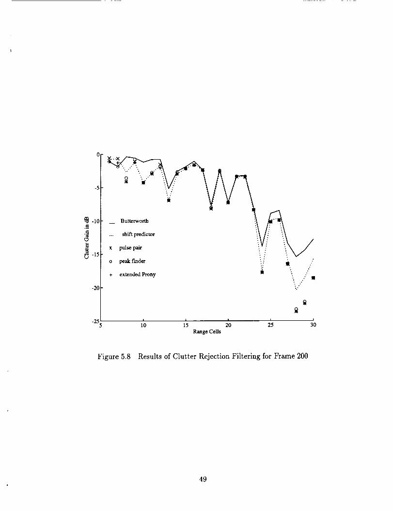
shifting occurs in the closer range cells. Figure 5.8 shows the clutter rejection filter

gain for the five filtering schemes: the Butterworth notch, the shift predictor centered

notch, tile pulse pair centered notch, the peak finder centered notch, and the extended

Prony centered notch. This gain is the ratio of output power to input power expressed

in dB over the entire processing bandwidth. Thus the better the clutter rejection the

lower the gain value. Notice that overall tile complex filter schemes do better than the

Butterworth filter at rejecting clutter. At all the ranges shown except for the closest

ranges at range cells 6 and 7, the clutter rejection of each complex filter is greater

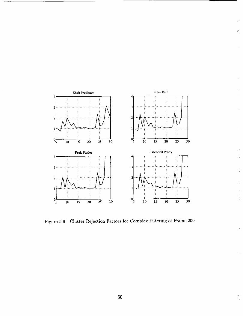
than or equal to that of the Butterworth filter. Figure 5.9 shows how each complex

filter performs relative to the performance of the Butterworth filter. The comparison

of the complex filter with the Butterworth filter is made by taking the power out after

using the Butterworth clutter rejection filter divided by the power out after filtering

with the complex filter. The resulting ratio is called the clutter rejection factor and

shows more of an improvement tile larger the number. For a factor greater than one

the complex filter rejects more clutter power than the Butterworth filter, and for a

factor less than one the Butterworth filter rejects more clutter.

48

-5

-I0

L3

-15

-2O

"_ ...'".. .-" ...

But .orth'x,,,,...i, i"/%/o peak f'mder : •

• " _ ,'

+ extended Prony i :- :"- ," m•, .,"

:.,"

! !

-255 10 15 2'0 2'5 30

Range Cells

Figure 5.8 Results of Clutter Rejection Filtering for Frame 200

49J

Shift Predictor

if.......i.......i.......i............

5 10 15 20 25 30

4

3

2

1

05

Pulse Pair

10 15 20 25 3O

Peak Finder

4 . , , :

3 ....... ! ....... {....... ! ........ i.......

2 ...... :.......!.......i...... i.......

lO " "''"

5 10 15 20 25 30

Extended Prony

5 10 15 20 25 3O

Figure 5.9 Clutter Rejection Factors for Complex Filtering of Frame 200

0 : _

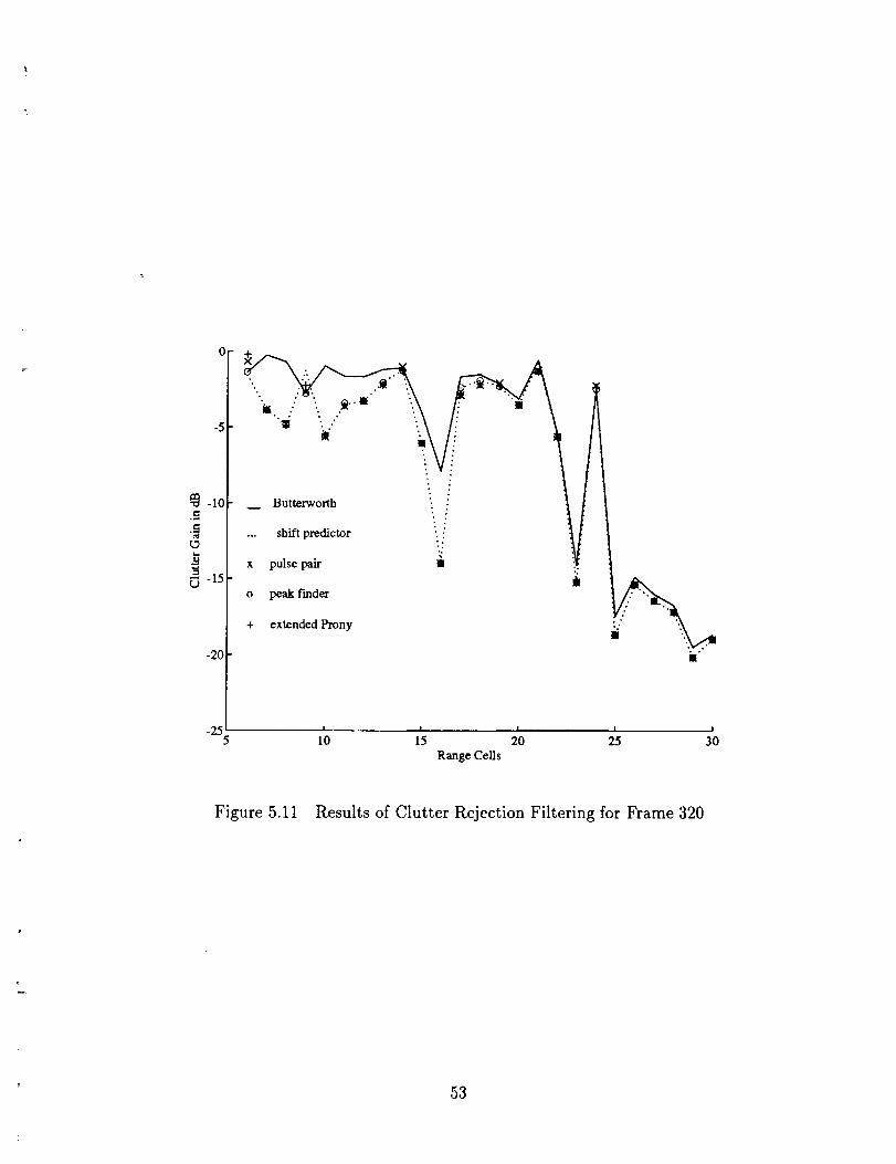
Figures 5.10 and 5.11 show the clutter gains for Frames 270 and 320 respectively.

In each case, all of the filters reject more of the clutter power in returns from

longer ranges. In the individual range cell spectra for Frame 270 in Appendix B,

the clutter mode can be seen to be more spread at the closer ranges than at ranges

that are farther away. When the clutter power becomes more concentrated around

a central frequency, all of the clutter rejection filters are able to cancel more of that

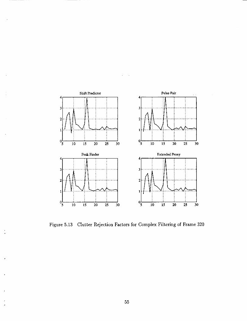
power. The clutter rejection factors in Figures 5.12 and 5.13 show similar results for

Frames 270 and 320. The clutter rejection factors for Frame 270 demonstrate that

clutter spectrum spreading at closer ranges reduces the ability to estimate a useful

clutter mode shift for the complex filtering routine.

From these results, filtering with a complex filter seems to improve the ability to

reject clutter power in the close range cells when a definite clutter mode shift can be

identified. The cases in which the complex filter does not improve on the Butterworth

filter have a clutter spectrum lacking a dominant mode which can be identified as the

major source of clutter power in the return spectrum. In general, the complex filter

does a good job of improving clutter rejection.

In terms of the clutter rejection factors, the shift predictor seems to be a poor

estimator for the clutter mode shift. As mentioned before, the shift predictor is mainly

limited by the theory that sidelobe returns are the only reason for the clutter mode

shift in the near ranges. It appears that there is more going on than just sidelobe

returns, and the tracking method of the shift estimators seems to be a more robust

method for estimating the clutter mode shift than predicting it based on just the

aircraft and antenna positions.

As can be observed in the range cell spectra in Appendix B, the closer range cells

contain more low level returns that are spread in frequency than the farther range

cells. After about range cell 25 the return spectra tend to show more of a dominant

mode with the returns at other frequencies decreasing in power. For this reason the

51

-2

-4

_6 ¸

rb -8

-I0

-12

-14

-16

Butterworth

... shift predictor

x pulse pair

Range Cells

Figure 5.10 Results of Clutter Rejection Filtering for Frame 270

52

i x+'"it .:: "., ._'"

_ ""_ :, ." '.

-10

-is

-2025 210 _ ill' 3;

Range Cells

Figure 5.11 Results of Clutter Rejection Filtering for Frame 320

53

Shift Predictor4 ,

I

05 ,o ,'5 io 25 3o

PulsePair

4

3 ........ i ....... •....... _........ .......

1

5 I0 15 20 25 30

Peak Finder

4 : f .... : :

3 .......!.......!.......i........i.......

2 .......i.......!.......!....... i.......

,o.5 I0 15 20 25 30

Extended Prony

:F....i.......J.......i........,.......2 ....... ! ....... ! ....... -.'....... i.......

1 .......i-.. . . i

5 I0 15 20 25 30

Figure 5.12 Clutter Rejection Factors for Complex Filtering of Frame 270

54 "

Shift Predictor

5 10 15 20 25 30

Pulse Pair

5 I0 15 20 25 30

Peak Finder

3

Extended Prony

3

2

1

5 I0 15 20 25 30 5 I0 15 20 25 30

Figure 5.13 Clutter Rejection Factors for Complex Filtering of Frame 320

= 55

clutter gain of all of the filters showa greaterattenuation whenthe dominant mode

is present.

An important factor to consideris whetherthe improvedclutter rejection is worth

the addedcomputational load necessaryto implement the complexfiltering scheme.

Although at farther rangesthe clutter gain of filtering showsa greater attenuation,

the decreasedattenuation at closerrangesis partly due to the fact that the signal

level in these rangesis already low. A more important factor at the closerranges

is the "whiteness"of the clutter spectra. From the rangecell spectraof Frame270

in Appendix B, the closerrangecells showa lack of any spectral mode. Sincethere

is no dominant mode, filtering at different Doppler frequenciesdoesnot result in

any improvement in clutter rejection. With the low power level and the spectral

whitenessin the closerrangecells,the computationnecessaryto searchfor a possibly

nonexistentclutter modedoesnot seemto bea worthwhile cost. Thus the fixednotch

at zeroDoppler is probably a better choice.

56

CHAPTER 6

CONCLUSIONS

The ability of an airborne radar to correctly identify desired targets is very closely

tied to its ability to successfully reject the clutter that appears in the return signal.

For an airborne weather radar in the "lookdown" position, the strongest clutter return

will be from the ground. Since the most common form of clutter rejection filter is a

filter with a rejection notch centered at zero Doppler frequency (aircraft groundspeed),

the successful rejection of ground clutter power depends on the ability of the receiver

to center the clutter spectrum at zero frequency.

In theory there should be a main lobe clutter shift at close ranges based on the

way the return spectrum is centered. For ranges less than the antenna boresight

range to the ground, the dominant clutter is from sidelobes and is shifted away from

the aircraft groundspeed. Since this shift is due to returns outside of the main lobe

of the radar beam, the clutter returns at short ranges are attenuated by the reduced

antenna gain. Because the clutter is at such a relatively low level, this predicted

clutter shift should not be a real problem for the conventional clutter rejection filter.

For a lookdown radar centering is accomplished based on the antenna azimuth

and tilt angles. When a clutter mode shift due to sidelobe returns occurs, there are

at least three options which can be taken to possibly improve clutter rejection. One

option is to center the clutter mode by using the complex demodulation process to

shift the entire spectrum. After filtering with a zero centered notch filter, the entire

spectrum would need to be shifted back to its original position in order to remove

possible aliasing effects. Such a procedure requires a method of estimating the shift

of the clutter mode.

A second option which is the topic of this study is to use a filter with complex

coefficients which allows for the capability of locating the filter notch at the Doppler

position of the main clutter mode. The designof the complex coefficientfilter is a

simple procedure. It turns out that the majority of the computation time is spent

on figuring out whereto movethe filter notch. Presentedwerethree shift estimators

and onepredictor. The shift predictor basesits estimationof the shift locationon the

position data of the aircraft and the radar antenna. Sucha predictive estimation is

limited by the theory that the aircraft and antennapositioningare the only variables

involved in the clutter mode shift, which cannot be proven to be true. The three

shift estimatorsare the peakfinder, the pulsepair estimator, and the extendedProny

analysis,and while eachhas its drawbacks,they all do a fairly goodjob of tracking

the clutter mode.

The complexfilter is a simple tool which could be useful in other applications.

The useof the complexfilter in the rejectionof discreteclutter could be effectivede-

pending on the algorithm for identifying suchclutter. The principlesof the extended

Prony analysisseemto havepotential use for clutter rejection filtering and possibly

evenfor discreteclutter rejection. It would appearthat increasingthe AR model to

at least order 3 couldpossiblyallow for the identification of discreteclutter basedon

the logic usedin previous research[6]. Further investigation would be necessaryin

order to find out if sucha theory is feasible.

Another possibleoption for the compensationof the clutter mode shift is to

implement a filter with a varying notch width. The width of the clutter rejection

filter could be dependenton the spreadof the clutter spectra. Sucha variable width

filter could even be implementedin conjunction With a complexfilter. The useof

sucha filter in the rejectionof clutter power is a topic for future study.

58

:z

f

APPENDICES

\

59

Appendix A

Levinson-Durbin Algorithm

Autoregressive(AR) modeling hasbeenrecognizedas an appropriatemeansof

modeling the clutter in the airport terminal area. A study performed by Keel [11]

investigatesthe useof the AR processto supportan adaptiveclutter rejectionfiltering

scheme. Using the AR model for spectral estimation has been popular due to its

relatively low computational load requiredand an improvedspectral resolution over

conventionalFFT approaches.An AR model is an all pole model with the spectral

density0-2At

PAR(f) = p 2 (A.1)

1 + _ a_exp(-jZTrfiAt)i=l

where At is the sampling interval of the process, {ai} are the AR coefficients, and a 2

is the variance of the input white noise process. For a model of order p, the estimation

of the parameters {al, as,..., %, a s} is required where it is possible for p to be any

positive integer. One method of estimating these parameters is the Levinson-Durbin

algorithm which is an efficient method of solving a matrix equation.

The Yule--Walker equations relate the coefficients {ai} of the AR model to the

autocorrelation process of the signal R**(k) [33]. The AR coefficients can be obtained

by solving

= - Ei=l aiR_(k - i) + k = 0 (A.2)R_(k) = - _x aiR,_(k - i) l <_ k <_ N

which in matrix form is described by

R_(0) R_(-1) ... Rx_(-p)

R_,(1) R,_(0) .-. R_(-(p-1))

n_(p) n_(p-1).., n_(0)

1

al

ap

0.2

0

0

The autocorrelation estimate R_,(k) of the complex series x,_ is given by

1 N-k-1

n=O

(A.3)

(A.4)

I-

|

E

The Levinson-Durbin algorithm uses a recursive method of solving for the param-

eter set of the desired order model. For the pth order model the parameter set is

{%l,%2,...,%p,a_} where aki refers to the ith coefficient of a kth order model.

Starting with the first order parameters

R_(1)

an = R_(0)

a_ = (1 -laHI2)R_(O) (A.5)

the higher order parameters are recursively computed by the following:

]0"_¢-1 /----1

ak-l,i + akka*k_l,k__

a_ = (1 -[a_kl2)a___ . (A.6)

By recursively solving for the model coefficients, the Levinson-Durbin algorithm gives

the coefficients for all order models up to the desired order.

Ik

61

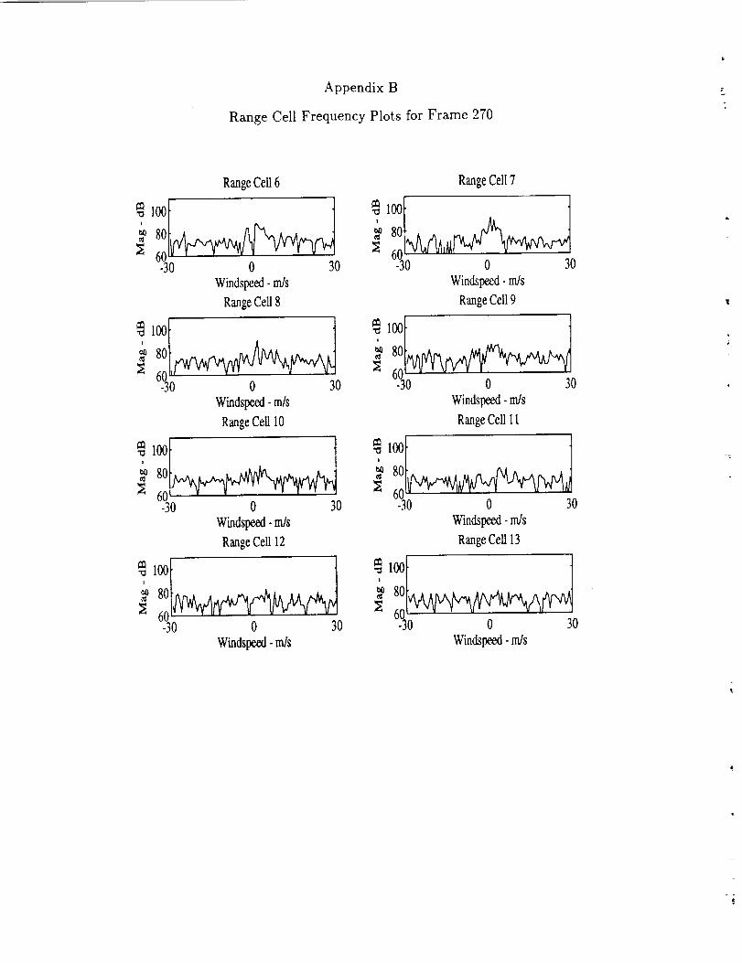
Appendix B

RangeCell FrequencyPlots for Frame270

RangeCell6 RangeCell7

8060-30 0 30

Windspeed - mJs

Range Cell 8

_ 100L_80

6-030 0 30

Windspeed - m/s

Range Cell 10

80

60-30 0 30

Windspeed -m/s

Range Cell 12

80

60-30 0 30

Windspeed -m/s

80

600 0 30

Windspeed - m/s

Range Cell 9

8O

60-30 0 30

Windspeed - m/s

Range Cell 11

_ 80

N 6O-30 0 30

Windspeed - m/s

Range Cell 13

80

60-30 0 30

Windspeed - m/s

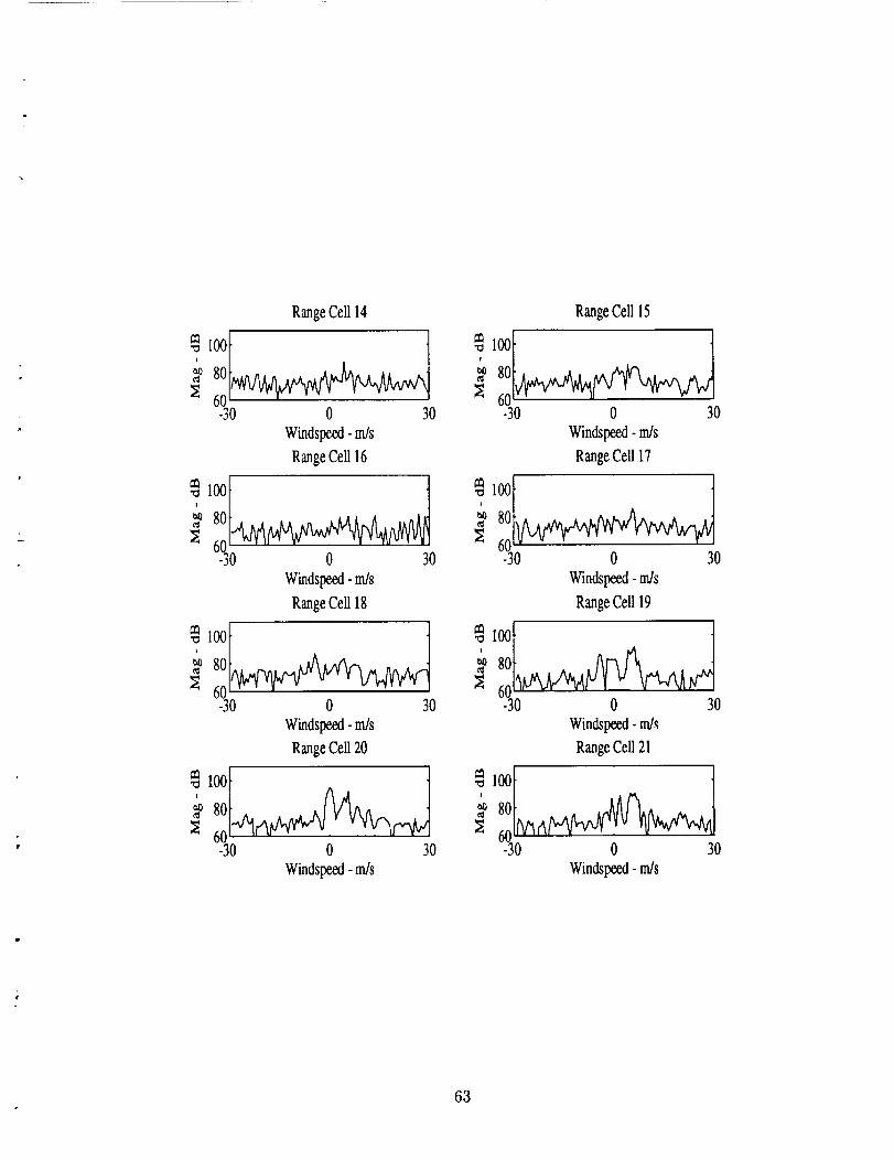
RangeCell14

8060-30 0 30

Windspeed-m/sRangeCell16

*1°°f.__80

6-_0 0 30

Windspeed - m/s

Range Cell 18

80

60-30 0 30

Windspeed - m/s

Range Cell 20

80

60-30 0 30

Windspeed - m/s

RangeCell 15

_ 8o_ 6O

-30 0 30

Windspeed - m/s

Range Cell 17

_ 80

6-_0 0 30

Windspeed - m/s

Range Cell 19

80

60-30 0 30

Windspeed -m/s

Range Cell 21

80

0

Windspeed - rials

63

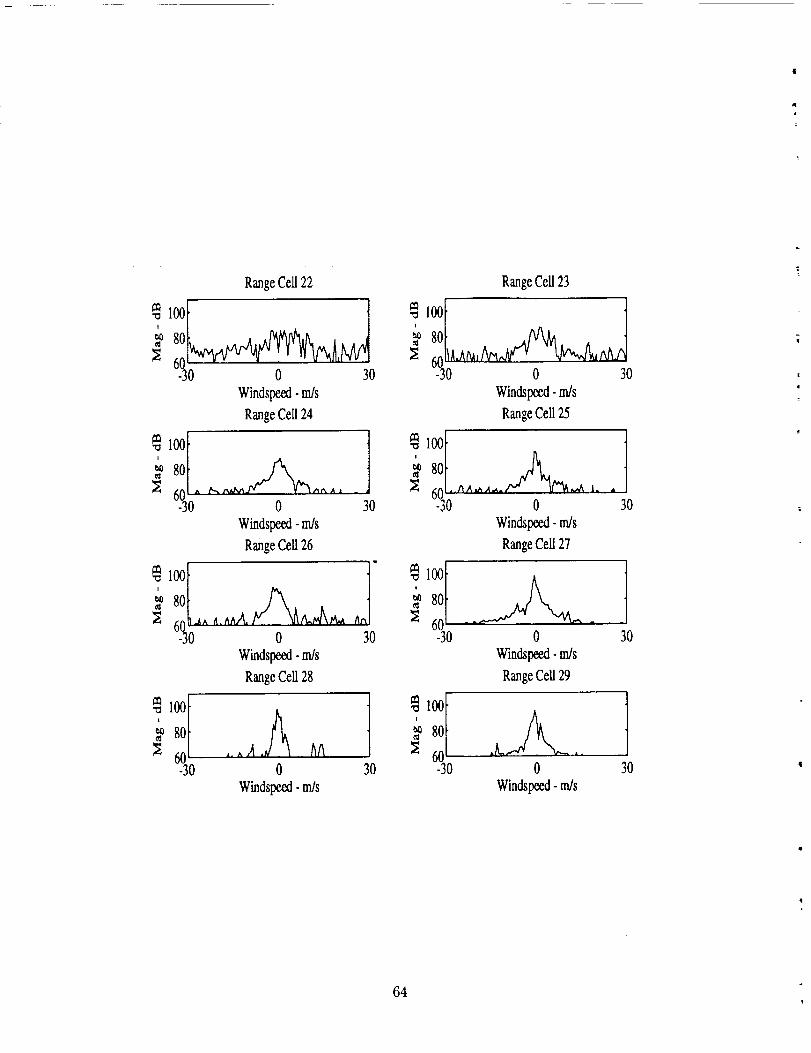
RangeCell22

1°°I_ _80

60-30 0 30

Windspeed- m/s

RangeCell24

80

- 0

Windspeed- m/s

RangeCell26

30

80

60 .4A _.^hA. A_ ^,_0 30

Windspeed- m/s

RangeCell 28

-30

f80

60 ,.,,A. AA-30 0

Windspeed- m/s

30

RangeCell 23

_1°°I,80

60 ^,A/U,/_ NL/'-30 0 30

Windspeed- m/s

RangeCell 25

80

-30 0

Windspeed- m/s

RangeCell 27

30

80

60 .....-30 0 30

Winctspeed- m/s

RangeCell29

l80

60 .L ,.-30 0

Windspeed- m/s

30

64

Range Cell 30

80

60-30 0 30

Windspeed -m/s

Range Cell 32

80

60-30 0 30

Windspeed - m/s

Range Cell 34

80

60-30 0

Windspeed -m/s

Range Cell 36

30

80

60-30 0 30

Windspeed - m/s

f80

60

Range Cell 31

-30 0 30

Windspeed - m/s

Range Cell 33

80

60-30 0 30

Windspeed - m/s

Range Cell 35

80

60-30 0 30

Windspeed - m/s

Range Cell 37

80

60"-30 0 30

Windspeed - m/s

65

RangeCell 38

8060 '-30 0

Windspeed - m/s

Range Cell 40

80

_ 6__ " 0

Windspeed - m/s

Range Cell42

30

30

8060-30 0 30

Windspeed - m/s

Range Cell 44

30

t80

-30 0

Windspeed - m/s

_1oo]8060

Range Cell 39

-30 0 30

Windspeed -m/s

RangeCell 41

80

6-" --- 0 30

Windspeed - m/s

Range Cell 43

_ 8o60-30 0 30

Windspeed - m/s

Range Cell 45

8060 "" "_"-30 0

Windspeed - m/s

66

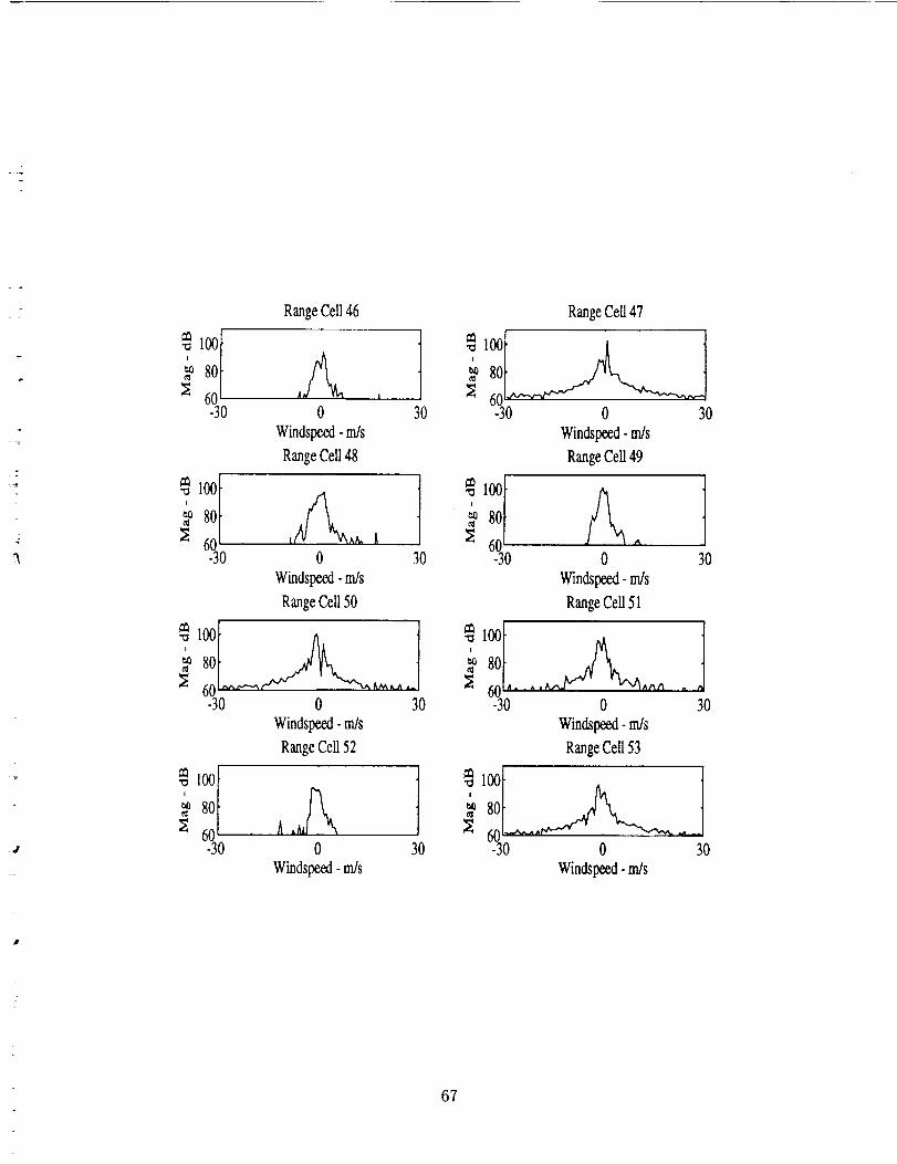
RangeCell46

8060 A ,-30 0

Windspeed-m/sRangeCell48

806 _ _.A- 0

Windspeed-m/s

RangeCell 50

80

-30 0

Windspeed - m/s

Range Cell 52

t80

60-30 0

Windspeed - m/s

30

30

A.

30

30

Range Cell 47

80

6-_0 0 %0

Windspeed - m/s

Range Cell 49

80

60 ^-30 0

Windspeed - m/s

Range Cell 51

N 60,, .... ^,_^..

30

-30 0 30

Windspeed - m/s

RangeCell 53

_ lOOI_ __ 8O

60 ....-30 0 30

Windspeed - m/s

67

RangeCeU54

1oo[80

60-30

_A ....

0

Windspeed - m/s

Range Cell 56

'_ 80

N 6°

_h

0

Windspeed - m/s

Range Cell 58

30

30

1oo]80

60 ....-30 0

Windspeed - m/s

RangeCeU60

1oo[80

60-30 0

Windspeed -m/s

30

Range Cell 55

80

60 .....-30 0

Windspeed - m/s

Range Cell 57

8060 ..... ^" "--30 0

Windspeed - m/s

Range Cell 59

30

L8060-30 o

Windspeed - m/s

Range Cell 61

30

30

80

6030-30 0

Windspeed - m/s

m

68

RangeCell62

f 8O

-30 0 30Windspeed-m/sRangeCell 64

_1°°l8060-30

_1°°I80

60

_1°°l8060-30

-30

_1°°L80

60-30

I _'°°I_ 80

0 30 -30

Windspeed - m/s

Range Cell 66

80

" " ' _ 600 30 -30

Windspeed - m/s

Range Cell 68

0

Windspeed - m/s

Range Cell 63

30

0

Windspeed - m/s

Range Cell 65

0

Windspeed - m/s

Range Cell 67

_1oo[8060

0

Windspeed - m/s

Range Cell 69

-30 0

Windspeed - m/s

30

30

30

30

69

RangeCell 70

f80

60-30 0

Windspeed - m/s

Range Cell 72

30

80

60-30 0

Windspeed - m/s

Range Cell 74

30

100i

80

60-30 0

Windspeed -m/s

Range Cell 76

30

80

60-30 0 30

Windspeed - m/s

Range Cell 71

f80

60 .......-30 0

Windspeed - m/s

Range Cell 73

30

80

60-30 0

Windspeed -m/s

RangeCell 75

30

_1°°t80

60-30

• . _ i ,

0 30

Windspeed - m/s

Range Cell 77

,,_,A__ .]_1oo[80

60---30 0 30

Windspeed - m/s

70

RangeCell78

_1_f8060-30

80

_6.

0

Windspeed - m/s

Range Cell80

./'1.

30

0

Windspeed - m/s

Range Cell 82

80

6 0

Windspeed -m/s

Range Cell 84

_°°I80 _,_

-30 0

Windspeed - m/s

30

30

_1oo]80

60-30

_1oo[8060-30

_1_I8060""-30

_1°°f8060-30

Range Cell 79

0

Windspeed - m/s

RangeCell 81

30

A0 30

Windspeed - m]s

Range Cell 83

0

Windspeed - m/s

Range Cell 85

0

Windspeed - m/s

30

30

71

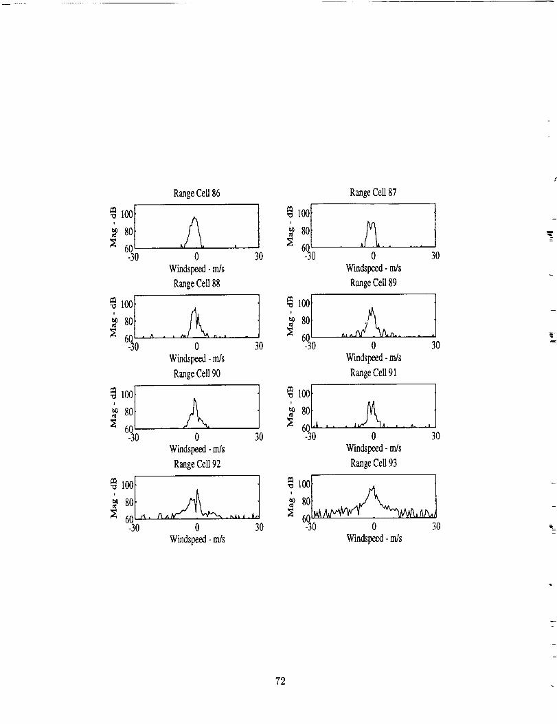
100I

80

60-30

80

_6 "_'

80

_ 6

80

60 .c_,-30

RangeCell86

0

Windspeed- m/s

RangeCell88

30

• /'_ll ',o. rl, i .

0

Windspeed- m/s

RangeCell90

30

0

Windspeed- m/s

RangeCell92

30

0 30

Windspeed- m/s

RangeCell87

I80

60 . A ---30 0

Windspeed- m/s

RangeCell 89

30

f80

60 "' "JV'/ '_--30 0

Windspeed-m/s

RangeCell 91

30

_1oo]80

60,A ,. . , , .....-30 0

Windspeed- m/s

RangeCell93

.I.

30

I80

60 _ _v/L t_/"u_-30 0 30

Windspeed- m/s

72

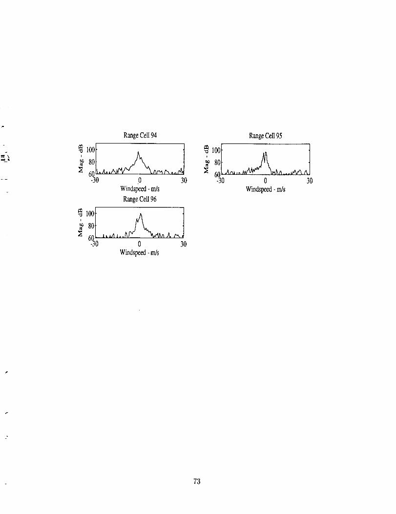
Range Cell94

_ 8o

-30 0 30

Windspeed - m/s

Range Cell 96

_1°°I80

60-30

l,_ l,.A_a A r',.

0 30

Windspeed - m/s

RangeCell 95

I_ 8o60 .A,-,,,,, _a._.,J_v'_ ^-30 0

Windspeed - m/s

30

73

REFERENCES

1. M. I. Skolnik, editor. Radar Handbook. McGraw-Hill, New York, 1990.

2. G. V. Morris, editor. Airborne Pulsed Doppler Radar. Artech House, Norwood,

Massachusetts, 1988.

3. S. A. Hovanessian. "Medium PRF Performance Analysis". IEEE Trans. on

Aerospace and Electronic Systems, vol. AES-18, May 1982, pp. 286-296.

4. W. W. Shrader and V. G. Hansen. "New Clutter Rejection Waveforms for Long-

Range Radar". IEEE Trans. on Aerospace and Electronic Systems, vol. AES-16,

November 1980, pp. 763-770.

5. F. W. Sears, M. W. Zemansky, and Young H. D. University Physics. Addison

Wesley, Reading, Massachusetts, 1987.

6. M. W. Kunkel. "Spectrum Modal Analysis for the Detection of Low-Altitude

Windshear With Airborne Radar". NASA CR-4457, August 1992.

7. W. T. Davis. "The Effects of Clutter-Rejection Filtering oll Estimating Weather

Spectrum Parameters". NASA CR 186212, July 1989.

8. D. S. Zrnid. Estimation of spectral moments for weather echoes. "IEEE Trans-

actions on Geoscience Electronics", vol. GE-17, 1979, pp. 113-128.

9. E. G. Baxa, Jr. and J. Lce. "The Pulse Pair Algorithm as a Robust Estimator of

Turbulent Weather Spectral Parameters Using Airborne Pulse Doppler Radar".

NASA CR-186792, February 1991.

10. D. D. Aalfs. "Real Time Processing of Radar Return on a Parallel Computer".

NASA CR-4456, July 1991.

11. B. M. Keel. "Adaptive Clutter Rejection Filters for Airborne Doppler Weather

Radar Applied to the Detection of Low Altitude Windshear". NASA CR 186211,

December 1989.

12. E. G. Baxa, Jr. "Airborne Pulsed Doppler Radar Detection of Low-Altitude

Windshear -- A Signal Processing Problem". Digital Signal Processing, vol. 1,

no. 4, October 1991, pp. 186 197.

13. E. Bracalente. "Doppler Radar Results". NASA Conference Publication 10105,

DOT/FAA/RD-92/19-I, September 1992, pp. 115-140.

14. C. L. Britt. "Algorithm to Complensate for Clutter Velocity Offset in the Wind-

shear Radar". Tech. Memo. Project 3042-68, Research Triangle Institute, Re-

search Triangle Park, North Carolina, .June 1989.

74

15.

16.

17.

18.

19.

20.

21.

22.

23.

24.

25.

26.

27.

28.

Y. C. Lai and E. G. Baxa, Jr. "On the Application of the LMS-Based Adap-tive Noise Canceller in Nonstationary Environment Associatedwith AirborneDopplerWeatherRadar". In Proc. of 1993 IEEE Int. Conf. on Acoustics, Speech,

and Signal Processing, Minneapolis, April 1993.

L. C. Ludeman. Fundamentals of Digital Signal Processing. Harper and Row,

New York, 1986.

A. V. Oppenheim and R. W. Schafer. Discrete-Time Signal Processing. Prentice

Hall, Englewood Cliffs, New Jersey, 1989.

T. tt. Crystal and L. Ehrman. "The Design and Applications of Digital Filters

with Complex Coefficients". IEEE Transactions on Audio and Electroacoustics,

vol. AU-16, September 1968, pp. 315-320.

H. Iwakura. "New Frequency Transformations for Complex Digital Filters".

Electronics Letters, vol. 27, October 1991, pp. 2083-2085.

P. A. Regalia, S. K. Mitra, and J. Fadavi-Ardekani. "Implementation of Real

Coefficient Digital Filters Using Complex Arithmetic". IEEE Transactions on

Circuits and Systems, vol. CAS-34, 1987, pp. 345-353.

W. L. Mills, C. T. Mullis, and R. A. Roberts. "Digital Filter Realizations With-

out Overflow Oscillations". IEEE Transactions on Accoust., Speech Signal Pro-

cess., vol. ASSP-26, August 1978, pp. 334-338.

T. T. Fujita. "The Downburst". SMRP Research Paper No. 210, The University

of Chicago, 1985. (available from NTIS as PB85-148-880).

M. Eide and B. Mathews. "Acquisition and Use of Orlando, Florida and Con-

tinental Airbus Radar Flight Test Data". NASA Conference Publication 10105,

DOT/FAA/RD-92/19-I, September 1992, pp. 357-372.

R. L. Bowles and R. Targ. "Windshear Detection and Avoidance: Airborne

Systems Perspective". Presented at the 16 th Congress of the ICAS, Jerusalem,

Israel, August 28 - September 2, 1988.

R. E. Bach and R. C. Wingrove. "Analysis of Win&hear from Airline Flight

Data". J. Aircr., vol. 26, February 1989, pp. 103-109.

W. tl. [teiss, D. L. McGrew, and D. Sirmans. "Nexrad: Next Generation

Weather Radar (WSR-88D)". Microwave Journal, January 1990, pp. 79-98.

M. Michelson, W. W. Shrader, and J. G. Wieler. "Terminal Doppler Weather

Radar". Microwave Journal, February 1990, pp. 139-148.

J. Evans and D. Turnbull. "Development of an Automated Windshear Detection

System Using Doppler Weather Radar". Proceedings of the IEEE, vol. 77, no.

11, November 1989, pp. 1661-1673.

75

29.

30.

31.

32.

33.

J. McCarthy. "Advances in Weather Technology for tile Aviation System". Pro-

ceedings of the IEEE, vol. 77, no. 11, November 1989, pp. 1728-1734.

S. Campbell, A. Berke, and M. Matthews. "The Orlando TDWR Testbed and

Airborne Wind Shear Data Comparison Results". NASA Conference Publication

10105, DOT/FAA/RD-92/19-II, September 1992, pp. 811-846.

A. I. Mackenzie, E. G. Baxa, Jr., and S. D. Harrah. "Characterization of Urban

Ground Clutter with New Generation Airborne Doppler Weather Radar". In

Proceedings of 1993 IEEE National Radar Conference, Boston, April 1993.

S. Haykin, B. W. Currie, and S. Kessler. "Maximum Entropy Spectral Analysis

of Radar Clutter". Proceedings of the lEER, vol. 70, September 1982, pp. 953-

962.

S. M. Kay and S. L. Marple. "Spectrum Analysis--A Modern Perspective".

Proceedings of the lEER, vol. 69, no. 11, November 1981, pp. 1380-1419.

76

REPORT DOCUMENTATION PAGE IForm Approved

OMB No 0704-0f88

PuDhcreporting burden for this collection of informatqOn is eStbmRt?¢_tO average _ hour oer ,esDorse. including the time tot revlew_n_ _nstruCtlan% _earch_n,_ el st,ng data _our(E'sathefln and ma _ta_nlng the data needed, and completing ano rpvaew_ngthe collection of mformat_On Send comments regarding th_ burden estimate of an,_other asp'=ctof th_s

(g_Flecllogof _nformat_on, .nc_udqng suggestion_ for reducungth_, Durden to Wa_hmcJton _;eaclcluar{ers Ser_rces, _re_orate _or !rlforrnat_On ODe at C_ and Rep<_r%, 1215 _effer'_o_£)av;s Haghway. {;uite _204. Afhngton, V_ 22202-4302, _nd 1o th_ Office of _AanacJemer_ and Budge_ Paperwork Reducx,_Ot_Project (0704-01B81 Wash_n_t,_n c_C _0503

1. AGENCY USE ONLY (Leave blank) 2. REPORT DATE 3. REPORT TYPE AND DATES COVERED

October 1993 Contractor Report4. TITLE AND SUBTITLE 5. FUNDING NUMBERS

Designing Clutter Rejection Filters with Complex WU 505-64-12-02Coefficients for Airborne Pulsed Doppler Weather Radar

6. AUTHOR(S)

Dennis A. Jamora

7. PERFORMING ORGANIZATION NAME(S) AND ADDRESS(ES)

Radar Systems LaboratoryElectrical and Computer Engineering DepartmentClemson UniversityClemson, SC 29634-0915

9. SPONSORING/MONITORING AGENCY NAME(S) AND ADDRESS(ES)

National Aeronautics and Space AdministrationLangley Research CenterHampton, VA 23681-0001

G NAGI-928

8. PERFORMING ORGANIZATION

REPORT NUMBER

Technical Report #16

10. SPONSORING / MONITORINGAGENCY REPORT NUMBER

NASA CR-4550

DOT/FAA/RD-93/24

11. SUPPLEMENTARY NOTES

Langley Technical Monitor:Final Report

Anne I. Mackenzie

12a.DISTRIBUTION/AVAILABILITYSTATEMENT

Unclassified - Unlimited

Subject Category 03

12b. DISTRIBUTION CODE

13. ABSTRACT (Maximum 200 words)

Ground clutter interference is a major problem for airborne pulse Doppler radar operating atlow altitudes in a look-down mode. With Doppler zero set at the aircraft ground speed, groundclutter rejection filtering is typically accomplished using a high-pass filter with real valuedcoefficients and a stopband notch centered at zero Doppler. Clutter spectra from the NASAWind Shear Flight Experiments of 1991-1992 show that the dominant clutter mode can belocated away from zero Doppler, particularly at short ranges dominated by sidelobe returns.This report investigates use of digital notch filters with complex valued coefficients so that thestopband notch can be located at any Doppler frequency. Several clutter mode trackingalgorithms are considered to estimate the Doppler frequency location of the dominant cluttermode. From the examination of flight data, when a dominant clutter mode away from zeroDoppler is present, complex filtering is able to significantly increase clutter rejection over useof a notch filter centered at zero Doppler.

14. SUBJE_ TERMS

Doppler radar, clutterairborne weather radar

filtering, complex coefficients,

17. SECURITY CLASSIFICATIONOF REPORT

Unclassified

NSN 7540-01-280-5500

18. SECURITY CLASSIFICATIONOF THIS PAGE

Unclassified

15. NUMBER OF PAGES

8816. PRICE CODE

_05

19. SECURITY CLASSIFICATION 20. LIMITATION OF ABSTRAC1OF ABSTRACT

UnclassifiedStandard Form 298 (Rev 2-89)

Pr_r,bed by _NSI Std Z]B-IB29B-102