designing and prototyping of a transverse flux machine in...

Designing and prototyping of a transverse fluxmachine in soft magnetic composite using millingand turning techniques

Master’s thesis in Electrical power engineering

FELIX MANNERHAGEN

Electric Power Engineering at Energy and EnvironmentCHALMERS UNIVERSITY OF TECHNOLOGYGoteborg, Sweden 2017

MASTER’S THESIS IN ELECTRICAL POWER ENGINEERING

Designing and prototyping of a transverse flux machine in soft

magnetic composite using milling and turning techniques

FELIX MANNERHAGEN

Electric Power Engineering at Energy and EnvironmentCHALMERS UNIVERSITY OF TECHNOLOGY

Goteborg, Sweden 2017

Designing and prototyping of a transverse flux machine in soft magnetic composite usingmilling and turning techniquesFELIX MANNERHAGEN

c© FELIX MANNERHAGEN, 2017

Master’s thesisISSN 1652-8557Electric Power Engineering at Energy and EnvironmentChalmers University of TechnologySE-412 96 GoteborgSwedenTelephone: +46 (0)31-772 1000

Chalmers ReproserviceGoteborg, Sweden 2017

Designing and prototyping of a transverse flux machine in soft magnetic composite usingmilling and turning techniquesMaster’s thesis in Electrical power engineeringFELIX MANNERHAGENElectric Power Engineering at Energy and EnvironmentChalmers University of Technology

Abstract

In this thesis a polyphase claw pole machine has been designed, prototyped and verified throughmeasurements. The FE-calculation model have been verified against analytical calculations,there after the design have been changed through an iterative process to a more optimiseddesign. The machine have then been built in a soft magnetic composite, using milling andturning techniques. The techniques used to minimise the chapped edges is described. TheFE-calculated machine model is then verified against equal circuit parameters measurements,with a relative small error.

Keywords: Claw pole, transverse flux, electrical machine design, SMC, soft magnetic composite,prototyping, milling, turning

i

Preface

Acknowledgements

I would like to give a huge thank to my friend Isak Jonsson for the help with the mechanicalmanufacturing of this electrical machine, which made the prototyping possible.

iii

Contents

Abstract i

Preface iii

Acknowledgements iii

Contents v

1 Introduction 11.1 Accuracy description in text . . . . . . . . . . . . . . . . . . . . . . . . . . . . . . 11.2 Environmental aspect . . . . . . . . . . . . . . . . . . . . . . . . . . . . . . . . . . 1

2 Electromagnetic theory 22.1 Mathematical backround . . . . . . . . . . . . . . . . . . . . . . . . . . . . . . . . 22.2 Machine topology background . . . . . . . . . . . . . . . . . . . . . . . . . . . . . 62.3 Building aspects . . . . . . . . . . . . . . . . . . . . . . . . . . . . . . . . . . . . 92.4 Theory used in FE-calculations . . . . . . . . . . . . . . . . . . . . . . . . . . . . 9

3 Design 123.1 Verification . . . . . . . . . . . . . . . . . . . . . . . . . . . . . . . . . . . . . . . 123.2 Adding a magnet . . . . . . . . . . . . . . . . . . . . . . . . . . . . . . . . . . . . 153.3 Torque calculation . . . . . . . . . . . . . . . . . . . . . . . . . . . . . . . . . . . 163.4 Back-EMF calculation . . . . . . . . . . . . . . . . . . . . . . . . . . . . . . . . . 173.5 Final geometry . . . . . . . . . . . . . . . . . . . . . . . . . . . . . . . . . . . . . 183.6 Mechanical . . . . . . . . . . . . . . . . . . . . . . . . . . . . . . . . . . . . . . . 263.7 Thermal . . . . . . . . . . . . . . . . . . . . . . . . . . . . . . . . . . . . . . . . . 29

4 Prototyping 324.1 Rotor . . . . . . . . . . . . . . . . . . . . . . . . . . . . . . . . . . . . . . . . . . 324.2 Stator . . . . . . . . . . . . . . . . . . . . . . . . . . . . . . . . . . . . . . . . . . 344.3 Assembly . . . . . . . . . . . . . . . . . . . . . . . . . . . . . . . . . . . . . . . . 36

5 Measurements on prototype machine 395.1 Nominal torque . . . . . . . . . . . . . . . . . . . . . . . . . . . . . . . . . . . . . 395.2 Peak torque . . . . . . . . . . . . . . . . . . . . . . . . . . . . . . . . . . . . . . . 42

6 Analysis 466.1 Nominal torque . . . . . . . . . . . . . . . . . . . . . . . . . . . . . . . . . . . . . 476.2 Peak torque . . . . . . . . . . . . . . . . . . . . . . . . . . . . . . . . . . . . . . . 48

7 Conclusion 50

Appendices 52

v

1 Introduction

With the electrification of the automotive fleet, the demand on rare earth magnets has increased,since the most utilised type of machines for propulsion are permanent magnet machines whichtoday use relatively large volumes of neodymium for the magnets. Since neodymium is mainlymined in bad conditions [1], the increasing usage of rare earth materials may be harmful tothe environment [2], as well as to the health of the mine worker. One way to lowering the needfor rare earth magnets could be to utilise the reluctance torque in salient machines.

The electrical machine should be designed with the constraints to fit in a small single persontransportation vehicle, like a moped. The machine should be designed to deliver around 1 hpor 750 W at a rated speed of around 2500 rpm. The peak burst torque should be around15 Nm with a peak power output of 2 hp or 1500 W. The system voltage of the drivetrainshould be 48 V. The length constraint of the machine is that it should be shorter then 70 mm.

The machinability of soft magnetic composites has come a long way, which gives new possibili-ties for more complex geometries in electrical machine design. Larger fillets, larger cutout andthinner structures should be possible with the soft magnetic composite materials available today.

This thesis should deliver an understanding in the possibilities of electrical machines designsand the prototyping limitations in soft magnetic composite materials. The claw pole designshould give the possibilities for simpler winding structure without end-windings which givesthe possibility to have a shorter machine. The claw pole design could be a cheap alternative inthat manufacturing step compared to other machine topologies.

1.1 Accuracy description in text

All value accuracy shown in this thesis is written as Significant figures. Accuracy in analyticalcalculations is set from rounding errors. The accuracy in FE-calculation is derived fromconvergence dependency from the mesh refinement. Accuracy in measurements is set from theaccuracy in the measurements setup.

1.2 Environmental aspect

When sintering electromagnetic components from iron power, as is done in soft magneticcomposites, there is low to non waste of material, since the excess powder can be reused inthe next part [3]. The recycling of materials from parts made of soft magnetic composites isa fairly known process [4]. The part is crushed and the soft magnetic material is removedutilising the magnetic properties while the copper windings remain [5].

1

2 Electromagnetic theory

This section starts with the mathematical explanation of the dq-transform, the mathematicaldifferentiation of magnetic and reluctance torque and how the dq-currents can be used tocontrol the machine. The machine topology is briefly explained and some of the limitations ofthe manufacturing is presented. The section then ends with the theory used in the verificationof the FE calculations.

2.1 Mathematical backround

To be able to get the mathematical description of the machine in a more familiar form thedq-transform will be used. This subsection will go through the steps taken to derive thedq-parameters later used to design and verify the claw pole machine. The voltages in the3-phase system are expressed as

ua = Raia +dΨa

dt

ub = Rbib +dΨb

dt

uc = Rcic +dΨc

dt

(2.1)

The self-inductance of the stator windings is approximated as

laa = Laa0 + Laa2 cos(2θr)

lbb = Laa0 + Laa2 cos (2(θr − 120))

lcc = Laa0 + Laa2 cos (2(θr + 120))

(2.2)

Where Laa0 is the average value of the self-inductance and Laa2 is the amplitude of thevariations depending on rotor position. The mutual inductance between the stator windings isapproximated as

lab = lba = − (Lab0 + Laa2 cos (2(θr + 30)))

lbc = lcb = − (Lab0 + Laa2 cos (2(θr − 90)))

lca = lac = − (Lab0 + Laa2 cos (2(θr + 150)))

(2.3)

The flux linkage can then be expressed as

Ψa = laaia + labib + lacic + Ψm cos(θr)

Ψb = lbaia + lbbib + lbcic + Ψm cos(θr − 120)

Ψc = lcaia + lcbib + lccic + Ψm cos(θr + 120)

(2.4)

If the assumption that there is no zero component in the 3-phase system is used, the flux

2

linkage can be written as

Ψa =

(Laa0 + Lab0 +

3

2Laa2 cos(2θr)

)ia

+

√3

2Laa2 sin(2θr)(ib − ic) + Ψm cos(θr)

Ψb =

(Laa0 + Lab0 +

3

2Laa2 cos(2(θr − 120))

)ib

+

√3

2Laa2 sin(2(θr − 120))(ic − ia) + Ψm cos(θr − 120)

Ψc =

(Laa0 + Lab0 +

3

2Laa2 cos(2(θr + 120))

)ic

+

√3

2Laa2 sin(2(θr + 120))(ia − ib) + Ψm cos(θr + 120)

(2.5)

The voltage can then be described in a two-phase system by

uss = usα + jusβ =2

3(ua + ube

j 2π3 + uce

j 4π3 ) (2.6)

Equation (2.1) is then inserted in (2.6) which results in

uss = Rsiss + LdΨs

s

dt(2.7)

where Ψss is described as

Ψss =

2

3(Ψa + Ψbe

j 2π3 + Ψce

j 4π3 ) (2.8)

Equation (2.5) is then inserted in (2.8) and results in

Ψss = Lsiss + Ψme

jθr (2.9)

where Ψss is the total flux linkage, Ls is the Leakage and mutual inductance and Ψm is the

magnet flux linkage expressed in the αβ-system.The rotation of the rotor is then added to the equations as

uss = usejθr (2.10)


usejθr = Rsisse

jθr + LdΨs

s

dtejθr (2.11)

The chain rule is applied on (2.11) and results in

usejθr = Rsisse

jθr + LdΨs

s

dtejθr + jωrΨse

jθr (2.12)

The flux linkage from the rotational transformation looks like

Ψsejθr = (Laa0 + Lab0)ise

jθr +3

2Laa2e

j(2θr)(isejθr)∗ + Ψme

j(θr) (2.13)

3

which can be simplified to

Ψs = (Laa0 + Lab0)is +3

2Laa2e

j(2θr−2θr)is∗

+ Ψmej(θr−θr) (2.14)

Further simplified to

Ψs = (Laa0 + Lab0)is +3

2Laa2is

∗+ Ψm (2.15)

By separating the complex current the flux linkage looks like

Ψs = (Laa0 + Labo +3

2Laa2)isd + (Laa0 + Labo −

3

2Laa2)isq + Ψm (2.16)

were the complex inductance can be set to

Lsd = (Laa0 + Labo +3

2Laa2)

Lsq = (Laa0 + Labo −3

2Laa2))

(2.17)

By inserting (2.17) in (2.16) the total flux linkage becomes

Ψs = Lsdisd + jLsqisq + Ψm (2.18)

which inserted in (2.12) will result in

usd = Rsisd + Lsddisddt− ωrLsqisq

usq = Rsisq + Lsqdisqdt

+ ωrLsdisdωrΨm

(2.19)

which will describe the behavior of the permanent magnet machine with salient properties.From the equation system the equivalent circuit shown in Figure 2.1 is derived.

−

+

usd

isdRs Lsd

+−

ωrLsqisq

+−ωrΨm

+ −

ωrLsdisd

−

+

usq

isqRs Lsq

Figure 2.1: Eqvivalent circuit model

The shaft power can be calculated using

Pe =3ωr2· ImΨ∗s is (2.20)

where Pe is amplitude variant scaled. The torque can be calculated from

Te =3np2

(Ψmisq + (Lsd − Lsq)isdisq) (2.21)

4

d-Current [A]

q-C

urre

nt [A

]

Figure 2.2: Example on a MTPA curve

where the torque produced from the magnet is

Tm =3np2

(Ψmisq) (2.22)

and the torque produced from the salient properties is

Tr =3np2

((Lsd − Lsq)isdisq) (2.23)

From the torque equations it can be seen that both the magnetic- and reluctance torque isdependent of the q-current, but only the reluctance torque is dependent on the d-current. Tomaximise the output torque per ampere the combination of the isd and isq should be optimised.First the identification of isd and isq is done by

isd = Imag cos(β)

isq = Imag sin(β)(2.24)


Te =3np2

(ΨmImag sin(β) + (Lsd + Lsq)I

2mag sin(β) cos(β)

)(2.25)

Since the maximum Torque per ampere is of interest the derivative of (2.25) is taken and setequal to zero

dTedβ

=3np2

(ΨmImag cos(β) + (Lsd − Lsq)I2mag cos(2β)

)= 0 (2.26)

There after the cos(β) is solved for, this gives

cos(β) = − Ψm

4(Lsd − Lsq)Imag−

√1

2+

(Ψm

4(Lsd − Lsq)Imag

)2

(2.27)

A visualised example of the dq-current angle can be seen in Figure 2.2 where Lsd < Lsq, whichis indicated by the negative d-current.

5

2.2 Machine topology background

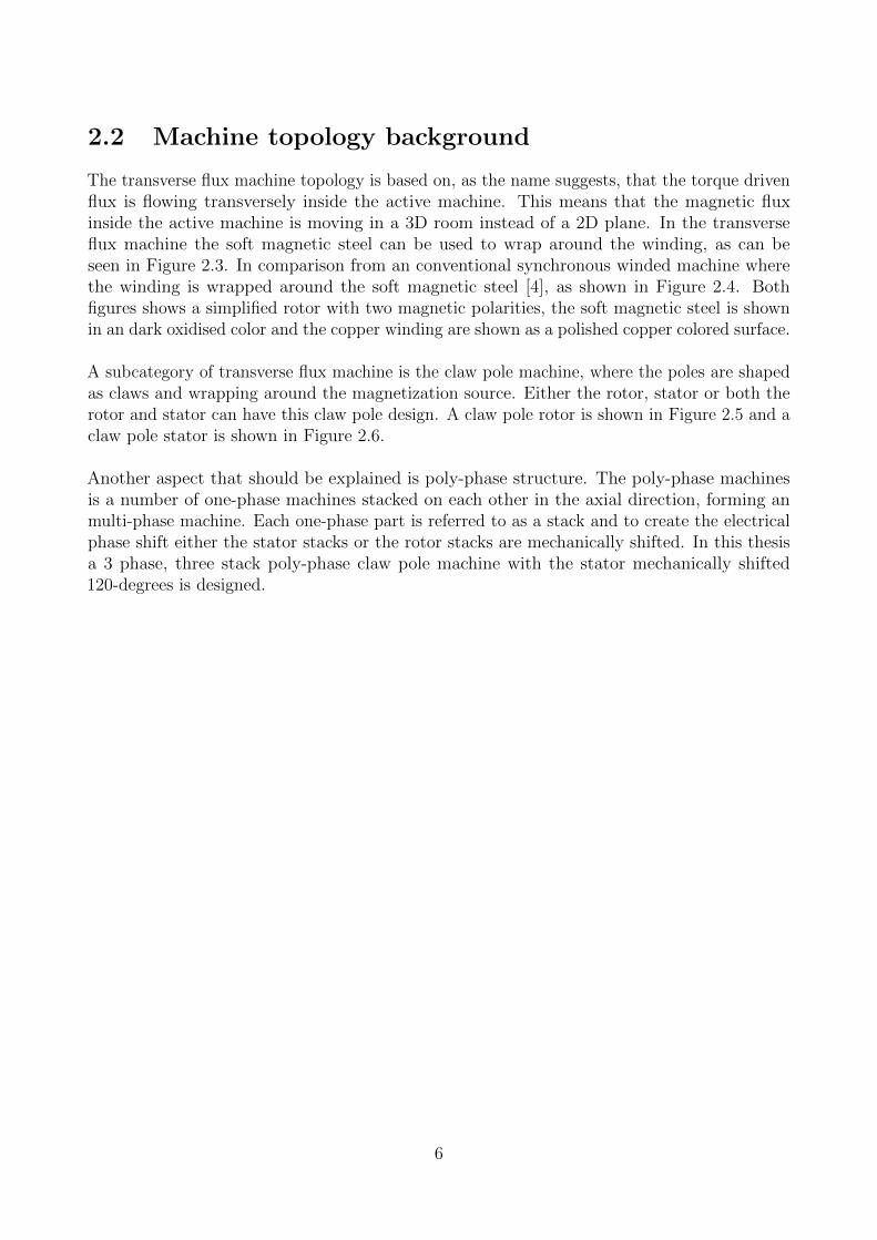
The transverse flux machine topology is based on, as the name suggests, that the torque drivenflux is flowing transversely inside the active machine. This means that the magnetic fluxinside the active machine is moving in a 3D room instead of a 2D plane. In the transverseflux machine the soft magnetic steel can be used to wrap around the winding, as can beseen in Figure 2.3. In comparison from an conventional synchronous winded machine wherethe winding is wrapped around the soft magnetic steel [4], as shown in Figure 2.4. Bothfigures shows a simplified rotor with two magnetic polarities, the soft magnetic steel is shownin an dark oxidised color and the copper winding are shown as a polished copper colored surface.

A subcategory of transverse flux machine is the claw pole machine, where the poles are shapedas claws and wrapping around the magnetization source. Either the rotor, stator or both therotor and stator can have this claw pole design. A claw pole rotor is shown in Figure 2.5 and aclaw pole stator is shown in Figure 2.6.

Another aspect that should be explained is poly-phase structure. The poly-phase machinesis a number of one-phase machines stacked on each other in the axial direction, forming anmulti-phase machine. Each one-phase part is referred to as a stack and to create the electricalphase shift either the stator stacks or the rotor stacks are mechanically shifted. In this thesisa 3 phase, three stack poly-phase claw pole machine with the stator mechanically shifted120-degrees is designed.

6

Figure 2.3: An example of an transversal flux machine

Figure 2.4: An example of a conventional radial flux machine

7

Figure 2.5: An example of an claw pole rotor

Figure 2.6: An example of an claw pole stator

8

2.3 Building aspects

The most common way of constructing an electrical 2D flux machine is by stacking laminatedsheets of electrical graded steel, this is done to decrease losses from eddy currents. There arethree main techniques that are used to cut out the geometry, stamping, water-jet cutting andlaser cutting. Stamping is used in mass production since the price per laminate is low but thedesign cost for stamping tools is high. Laser or water-jet cutting is mainly used for prototypingor small-scale production since the cutting speed is relatively slow and costly in comparison tostamping [6].

When the flux geometry changes from 2D to 3D the laminated sheet method may not beadequate to lowering the eddy currents. For 3D flux applications soft magnetic compositematerials is often used. For mass production soft magnetic composite material parts is usuallysintered into shape. But for prototyping or small series, the sintering method becomes expensivebecause of high tooling costs. For this reason companies like Hoganas have developed specialisedsoft magnetic prototyping materials, which makes drilling, turning and milling possible, seeapendix for datasheet. Even if the machinability of the soft magnetic prototyping materialis better than the conventional soft magnetic materials, there are some things that needs tobe considered. When milling, the tooling needs to be very sharp preferably new and unusedcarbide tools for aluminium or plastic. The material should always be supported, preferablyclimb milling used and cutting out of edges should be avoided. A common problem whenmachining soft magnetic materials is chapping, where edges is chipped and resulting in unevenedges.

2.4 Theory used in FE-calculations

In this subsection the basic behind the magnetic relations, later used to design and verifyingthe electrical machine, will be defined.

2.4.1 Reluctance torque

Assume that a coil is wounded around a ferromagnetic toroid with N number of turns and thecurrent I. This can be connected to the magnetic field intensity by Ampere’s circuital law as∮

c

H· dl = NI (2.28)

If the ferromagnetic toroid have a small air gap the magnetic field intensity differs in the airgap from the ferromagnetic material. The magnetic field intensity can be rewritten to magneticflux density using the constitutive equation

H =B

µ(2.29)

This is then set into (2.28) and integrated over the toroid with the mean radius r which results

9

in

B

µfe(2πr − lg) +

B

µ0

lg = NI (2.30)

After modification the result is

B =µ0µNI

µ0(2πr − lg) + µlg(2.31)

since the magnetic flux density is constant in the geometry the magnetic flux can be calculatedusing

Φ =

∫s

B · ds = BS (2.32)

Where S is the cross section area of the toroid. Equation 2.32 is then combined with (2.31)and results in

Φ =NI

(2πr−lg)µS

+ lgµ0S

(2.33)

This can then be rewritten as

Φ =NI

<fe + <g(2.34)

Were

<fe =2πr − lgµS

=lfµS

<g =lgµ0S

(2.35)

is the reluctance equations for the ferromagnetic geometry and the air gap. The inductancecan then be calculated using

L =NΦ

I=

N2

<fe + <g(2.36)

The force applied on the rotor equals to

F = ∆Wm = ∆Li2

2(2.37)

Equation (2.36) is then inserted in (2.37) to give the force dependent on the reluctance as

F =i2N2

2∆(<fe + <g)(2.38)

The total reluctance torque can then be approximated using

Tr ≈ nPFr (2.39)

where nP is the number of pole pairs, F the force and r rotor radius.

10

2.4.2 Magnetic torque

Since the magnetic path can be expressed as a magnetic circuit with two air gaps and tworeluctance paths as seen in Figure 2.7. With the approximation of the magnetic flux generatedfrom the permanent magnet to be constant, the total flux can be calculated as

Φtot = Φ + Φm (2.40)

were Φm is the magnetic flux generated from the permanent magnet.

<fe2

<g2

Φm

+−Vm

Φ

<fe2

<g2

Figure 2.7: Magnetic circuit model. Vm is the mmk and Φm the permanent magnet flux.

The magnetic work created with the permanent magnet flux can then be calculated as

Wm =iΦm

2(2.41)

The magnetic force is then calculated using

F = ∇Wm (2.42)

and the torque can then be calculated using

T = −∂Wm

∂θ(2.43)

11

3 Design

In this section the design specifications and limitations for the machine, will be derived andexplained. After that, the optimisation of the electromagnetic circuit is done. This is mainlydone by changing the geometry of the magnetic path, the size of the magnet and the numberof turns in the coil.

The limitations is mostly set by the delivered geometry of the soft magnetic material. Thematerial used is Somaloy prototyping material, the datasheet is included in the Appendix. TheSomaloy prototyping material is delivered as cylinders with a height of 20 mm and a diameterof 120 mm, which sets the geometrical limitations of the stator and rotor parts. The stackheight will therefore be set to be 20 mm and the stator outer diameter will be set to 120 mm.

The design process starts with analytical calculations, so that the setup for the FE calculationscan be verified. When the first verification is done, it is time to add the magnet to the machine.This is done by first calculating the size of the magnet, then adding the magnet into theFE calculations for detailed studies. When the FE calculations have been verified againstthe analytical calculations, then it is time to start to optimise by changing geometry andparameters. To be able to know what to change, the magnetic flux density plots are beingused, the high spots are being treated to lower the magnetic flux density and the material atlow spots are being removed to lower the weight of the machine and leakage inductance. Thenumber of turns in the winding is used to control the magnetic flux. When the electromagneticdesign is in a finished state, it is time to add the mechanical features needed to be able toassemble the machine. Finally a basic thermal simulation is done to find thermal limitations.

3.1 Verification

The inductance and resistance is chosen as the verification parameters, so for the verification,the inductance and resistance need to be calculated. Since the relation between inductance andreluctance is defined, in (2.36), the reluctance should be calculated. To be able to calculate thereluctance, the magnetic flux path needs to be defined. Therefore some initial values need tobe defined. As the initial values, the rotor diameter was set to half of the stator outer diameter,this results in a rotor diameter of 60 mm. The number of pole pairs was set to Np = 4, this wasdone since it seemed reasonable as an initial value. The air gap length was set to be 0.5 mmand the width of the teeth at the air gap was set to be the same width as the non aligned areacalculated as

teeth width =360

4Np

= 22.5 (3.1)

which will translate to mm by

s =22.5

180πr ≈ 11.8 mm (3.2)

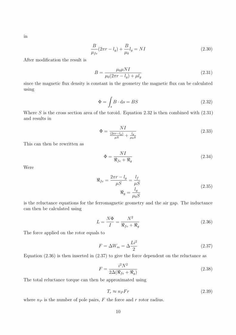
where r is the radius of the rotor. The verification geometry is shown in Figure 3.1. The arclength is then multiplied with the stack height to get the cross-section area of the air gap. Thecross-section area is then derived to

12

Figure 3.1: Rendering of the first iteration

a = sh = 236 mm2 (3.3)

The reluctance in the air gap can then be calculated using (2.35). The reluctance per air gapthen becomes

<g =lgaµ0

=0.5× 10−3

4π × 10−7 × 236× 10−6≈ 1.7× 106 (3.4)

The total reluctance depends on the pole pairs and is calculated as

<g tot =<gNp

=1.7× 106

4= 425× 103 (3.5)

The inductance contributed from the air gaps, is calculated as

Lg =N2

2<g tot=

102

2× 425× 103= 117.7 µH (3.6)

From the first FE calculation it could be seen that there was leakage inductance interferingwith the calculated inductance. The energy density plot of the FE calculation can be seen inFigure 3.2. It can be seen that there is magnetic energy behind the stator teeth and on theoutside of the air gap, which indicates that the fringing effects in this areas need to be considered.

First the inductance from the air gap needed to be calculated. This was done by setting therelative permeability to 4× 106 in the ferromagnetic material. The relative permeability ofthe copper windings and all air except in the air gap was set to 0.02, in order to decrease theinfluence of this regions. This gave a FE calculated inductance, L = 117.4 µH which can becompared to the calculated inductance of 117.7 µH, for the air gap.

13

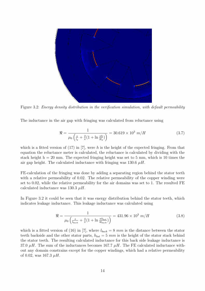
Figure 3.2: Energy density distribution in the verification simulation, with default permeability

The inductance in the air gap with fringing was calculated from reluctance using

< =1

µ0

(slg

+ 2π(1 + ln πh

2lg)) = 30.619× 103 m/H (3.7)

which is a fitted version of (17) in [7], were h is the height of the expected fringing. From thatequation the reluctance meter is calculated, the reluctance is calculated by dividing with thestack height h = 20 mm. The expected fringing height was set to 5 mm, which is 10 times theair gap height. The calculated inductance with fringing was 130.6 µH.

FE-calculation of the fringing was done by adding a separating region behind the stator teethwith a relative permeability of 0.02. The relative permeability of the copper winding wereset to 0.02, while the relative permeability for the air domains was set to 1. The resulted FEcalculated inductance was 130.3 µH.

In Figure 3.2 it could be seen that it was energy distribution behind the stator teeth, whichindicates leakage inductance. This leakage inductance was calculated using

< =1

µ0

(s

lback+ 4

π(1 + ln πhbst

4lback)) = 431.96× 103 m/H (3.8)

which is a fitted version of (16) in [7], where lback = 8 mm is the distance between the statorteeth backside and the other stator parts, hbst = 5 mm is the height of the stator stack behindthe stator teeth. The resulting calculated inductance for this back side leakage inductance is37.0 µH. The sum of the inductances becomes 167.7 µH. The FE calculated inductance with-out any domain constrains except for the copper windings, which had a relative permeabilityof 0.02, was 167.3 µH.

14

The leakage inductance contribution from the copper winding was calculated using a fittedversion of (15) in [7]. This resulted in a reluctance of

< =1

µ0

(wwinding2hwinding

+ 1π(1 + ln πhbst

2hwinding)) = 1.0733× 106 m/H (3.9)

were wwinding = 10 mm is the width of the winding, hwinding = 10 mm is the height of thewinding and hbst = 5 mm is the height of the stator stack behind the stator teeth. Since thisis in m/H the result was then divided with the interfering length which was calculated as

lcoil fringing = Obst − 2Nplteeth bst = 125.7 mm (3.10)

were Obst = 251.3 mm is the circumference behind the stator teeth, lteeth bst is the arc length ofthe teeth in the connection at the teeth and the stator base. The resulting leakage inductanceat the coil is 11.7 µH, which gives an total summed inductance of 179.4 µH. The FE calculatedinductance with defaulted domain and regions was 182.9 µH

With the fringing effects, defaulted domains and relative permeability and the relative per-meability of the ferromagnetic material was changed to 400, which is close to the maximumrelative permeability of the Material used. The calculated inductance become 140.8 µH andthe FE calculated inductance become 138 µH.

The winding resistance can be calculated using the resistivity of copper ρ = 1.68 × 10−8,the cross section area of the winding wire awire = 6.4 mm2, the length of one winding turnlwindingturn = 0.28 m and the number of turns N = 10. The winding resistance then becomes

R = N × ρlwindingawire

= 7.4 mΩ (3.11)

The FE calculated winding resistance was 7.4 mΩ, using the built in global evaluation for thecoil resistance in Comsol Multiphysics, which is equal to the calculated one.

3.2 Adding a magnet

The magnet needs to be added to the model to be able to verify the FE model against analyticalcalculations. The dimensions of the magnet is not important at this stage of the design, sincethe dimensions of the magnet will be changed in the iterative refinement process.

The height of the magnet is set to be 6 mm, and it will be buried 2 mm on each side to lowerthe magnetic flux density in the corners. Since there is going to be an axle through the magnetand the magnet needs to be magnetised in the axial direction, the magnet needs to have theshape of a cylinder with a center hole. Also the axle needs to be made of a nonmagneticmaterial like nonmagnetic stainless steel, with a relative permeability approximated to air.The radius of the axle is set to be 6 mm, since this is sufficient for the torque loads. For theverification the inner radius of the magnet is set to be 6 mm, the same as the radius of the axle.The outer radius is set to be 9 mm, half of the height of the magnet added on the inner radius.

15

3.3 Torque calculation

To be able to verify the FE calculations an analytical calculation on a torque step aroundaligned position was done. The torque was calculated using (2.43) were Wm = LI2

2and I was

set to 50 A. This then becomes

T = −∂L∂θ

I2

2(3.12)

Which is only valid in the simplified linear case with linear Media, which is used for thisverification. The variation of inductance at different angles was then calculated around thealigned position, with a step of 0.1 degrees. The change in inductance was calculated from thechange of the air gap cross section area depending on the angle. The inductance with fringingwas then calculated using the same method as for the verification of the inductance, where thespace for the magnet was added as a air gap of 2 mm since the other parts of the magnet wasburied 2 mm in the rotor parts and the magnet was 6 mm high. The width of the magnet was3 mm as calculated. Reluctance with fringing effect at the magnet was calculated using

< =1

µ0

(wmagnet

2hmagnet gap+ 1

π(1 + ln πhburied

2hmagnet)) = 0.92279× 106 m/H (3.13)

which is a fitted version of (17) in [7]. Since this gives the unit m/<, the result was thendivided with the outer circumference of the magnet, which was 56.6 mm. The inductance atdifferent angles was calculated and inserted into (3.12).

The analytical torque was constant, within the accuracy, around ±1 degree and equal to0.098 Nm. The plot of the analytical torque can be seen in Figure 3.3, when the fringing effectwas considered. Which can be compared to the FE calculated torque, which was 0.098 Nmaround ±1 degree.

16

Rotor angle [degree]-1 -0.8 -0.6 -0.4 -0.2 0 0.2 0.4 0.6 0.8 1

Tor

que

[Nm

]

-0.1

-0.08

-0.06

-0.04

-0.02

0

0.02

0.04

0.06

0.08

0.1

X: -0.95Y: 0.09795

Figure 3.3: The analytical torque at ±1 degree around aligned position

3.4 Back-EMF calculation

The analytical calculations of the Back-EMF was calculated using

emf = ωm∂Ψ

∂α(3.14)

where ωm is the mechanical angular frequency of the rotor and α = ωmt. Ψ is calculated asin (2.32) where B is the remanent flux density of the magnet and S the cross section area ofthe air gap. The cross section area was changed in the same way as for the torque calculations.The resulting back-EMF at 1 Hz was calculated to -4.2 mV at aligned position. Which can becompared with the FE calculated back-EMF which were -4.1 mV at aligned position, shown at0 degree in Figure 3.4.

17

Figure 3.4: The FE calculated back-EMF at 1 Hz with open coil terminals

3.5 Final geometry

Under several iterations, the geometry was changed to even out and lower spikes in the magneticflux density distribution. Fillets were added and changed to smother corners. The magnet sizechanged to an inner diameter of 25 mm, an outer diameter of 32.4 mm and a height of 6 mm.The magnet was buried 2 mm on each side in the rotor to lower magnetic flux density in thecorners. The magnets precise measurements was set by what was available at the manufacturerat that moment. The number of turns in the coil was changed to 13 turns and the crosssectionarea of the wire was changed to 1.1 mm2. The final mechanical geometry can be seen insection 3.6.

The phase resistance was FE-calculated to 62.5 mΩ. The inductance varies with rotor positionin a way that is shown in Figure 3.5. The average self-inductance was FE-calculated to 207.5 μH,and the varying inductance was FE-calculated to 97.5 μH. Since the FE-calculations have beendone in only one phase the mutual inductance was approximated to 0. The back-emf wasFE-calculated to 0.0206 V/Hz. This parameters were then transformed over to the dq-domainusing the method explained in 2.1 and can be seen in Table 3.1.

Table 3.1: FE-calculated parameters in the dq-domain

Rs 62.5 mΩLsd 354 μHLsq 61 μHΨm 0.0206 V/Hz

Since the equivalent circuit parameters is calculated, the dq-voltages and dq-currents can thenbe calculated using (2.19), by setting a maximum absolute voltage to 48 V and the currentangle equal to the MTPA angle shown in Figure 3.6.

18

Figure 3.5: FE calculated inductance curve for final geometry depending on mechanical rotorangle

d-Current [A]-150 -100 -50 0 50 100 150

q-C

urre

nt [A

]

0

20

40

60

80

100

120 Constant currentConstant torqueMaximum torque per ampere

Figure 3.6: The voltage components speed characteristics for MTPA calculated from FE-calculated values

3.5.1 Nominal torque

For the nominal torque the nominal current is 20 A and the current speed characteristics canbe seen in Figure 3.7, where the dq-components contributions is calculated from the MTPAangle. Figure 3.8 shows the voltage speed characteristics with the dq-component contribution.The absolute voltage and current speed characteristics is shown in Figure 3.9

The nominal torque is then calculated using (2.21), the magnetic torque contribution iscalculated using (2.22) and the reluctance torque contribution is calculated using (2.23). Thistorque contributions is then plotted against mechanical speed and is shown in Figure 3.10.The maximum nominal output power at different speeds is shown in Figure 3.11.

19

Mechanical speed [RPM]0 500 1000 1500 2000 2500 3000 3500 4000

Cur

rent

[A]

0

5

10

15

20

25

iisd

isq

Figure 3.7: Maximum current components speed characteristics for nominal torque


Vol

tage

[V]

0

5

10

15

20

25

30

35

40

45

50

uu

sd

usq

Figure 3.8: The voltage components speed characteristics for nominal torque

20


Vol

tage

[V],

Cur

rent

[A]

0

5

10

15

20

25

30

35

40

45

50

ui

Figure 3.9: Voltage and current per speed characteristics for nominal torque calculated fromFE-calculated values


Tor

que

[Nm

]

0

0.5

1

1.5

2

2.5

3

TT

m

Tr

Figure 3.10: Maximum nominal torque components at different speed calculated from FE-calculated values

21


Pow

er [W

]

0

100

200

300

400

500

600

700

800P

FE-calculated

Figure 3.11: Maximum nominal power at different speed calculated from FE-calculated values

22

3.5.2 Peak torque

For the peak torque the current is 100 A and the current speed characteristics can be seenin Figure 3.13, where the dq-components contributions is calculated from the MTPA anglein Figure 3.6. Figure 3.12 shows the voltage speed characteristics with the dq-componentcontribution. The absolute voltage and current speed characteristics is shown in Figure 3.14


Vol

tage

[V]

0

5

10

15

20

25

30

35

40

45

50

uu

sd

usq

Figure 3.12: The voltage components speed characteristics for MTPA calculated from FE-calculated values


Cur

rent

[A]

0

10

20

30

40

50

60

70

80

90

100

110

iisd

isq

Figure 3.13: Maximum current components speed characteristics for MTPA from FE-calculatedvalues

23


Vol

tage

[V],

Cur

rent

[A]

0

10

20

30

40

50

60

70

80

90

100

110

ui

Figure 3.14: Voltage and current per speed characteristics calculated from FE-calculated values

The peak torque is calculated in the same way as for the nominal torque case. This torquecontributions is plotted against mechanical speed and is shown in Figure 3.15. The maximumoutput power at different speeds is shown in Figure 3.16.


Tor

que

[Nm

]

0

2

4

6

8

10

12

14

16

18

20

TT

m

Tr

Figure 3.15: Maximum torque components at different speed calculated from FE-calculatedvalues

24


Pow

er [W

]

0

200

400

600

800

1000

1200

1400

PFE-calculated

Figure 3.16: Maximum power components at different speed calculated from FE-calculatedvalues

25

3.6 Mechanical

The geometry is developed to utilise the possibility to stack a common design on top ofeach other to create the final geometry. One rotor segment can be seen in Figure 3.17. Thepermanent magnet has a pocket to be lowered into, this gives the magnet more mechanicalstability and lower the magnetic stress in corners. The mechanical fastening between the rotorand the axle is done by using a key and keyway. Since the middle segment is turned upsidedown a design of the rotor part with the keyway angular shifted is needed. This makes thekeyway solution non fit for mass production since it duplicate the needs of tooling to sinter therotor. For prototyping purposes the keyway solution works fine, since the milling method is used.

Figure 3.17: Rendering of a rotor segment

The stator is mechanically held together with six threaded rods placed evenly through the outerrim, the mounting holes can be seen on a single stator part in Figure 3.18. This fastening alsofacilitates for an easy phase shift between each phase, since the stator needs to be mechanicallyshifted 120 electrical degrees which transfers to 60 mechanical degrees.

The 1 phase machine is then assembled as the exploded view shown in Figure 3.19. Wherethe winding is represented as a solid copper ring and the magnet can be seen as the shinystubby cylinder. The active machine assembly can be seen in Figure 3.20. In the stator the120 electrical degrees phase shift can be visualised by looking at the stator teeth. At therotor it can be seen that the middle segment is turned upside down, this is done to utilise themagnetic field so that each linked teeth have the same magnetic polarisation.

26

Figure 3.18: Rendering of a stator segment

Figure 3.19: Exploded view of 1 phase from left to right: stator segment, rotor segment, copperwindings, permanent magnet, rotor segment and stator segment.

27

Figure 3.20: Visualisation of the active 3 phase machine

28

3.7 Thermal

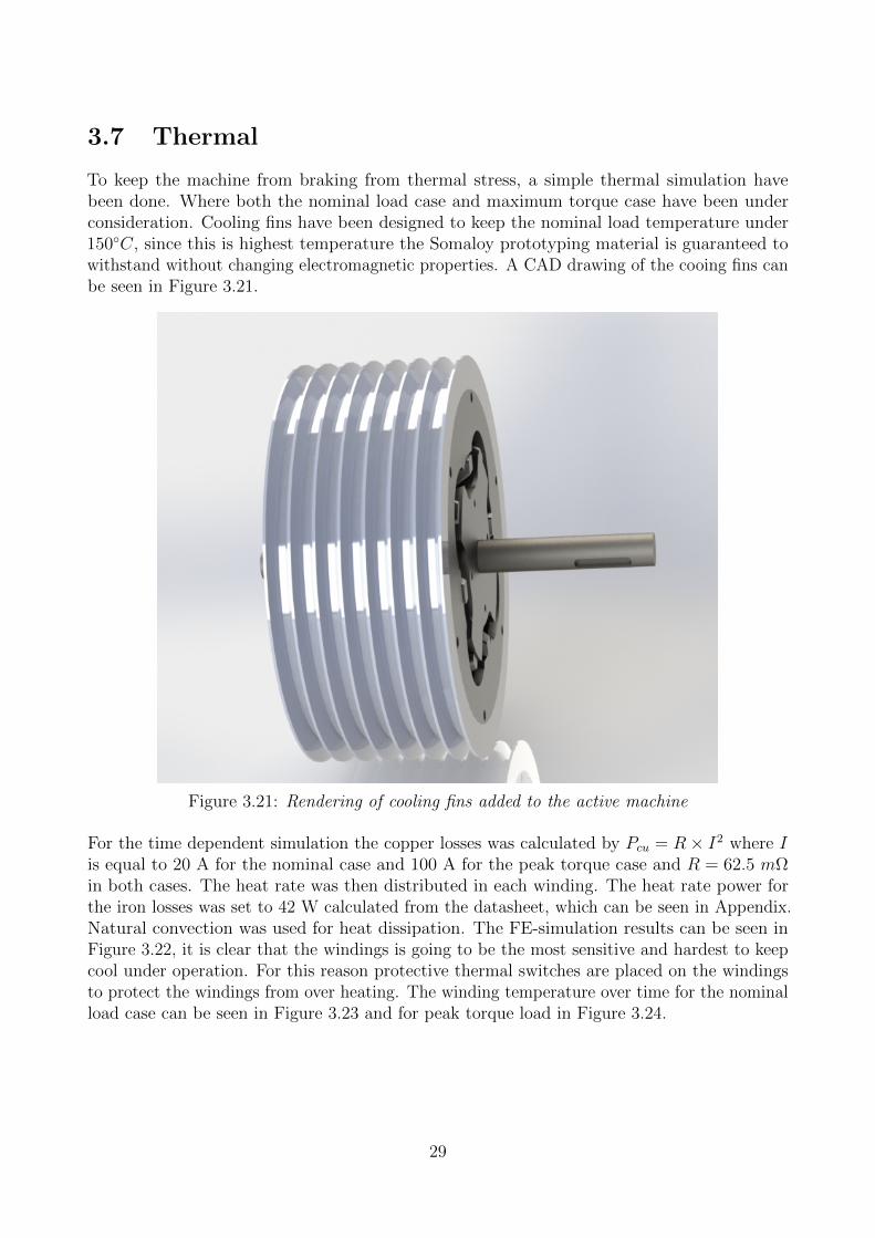
To keep the machine from braking from thermal stress, a simple thermal simulation havebeen done. Where both the nominal load case and maximum torque case have been underconsideration. Cooling fins have been designed to keep the nominal load temperature under150C, since this is highest temperature the Somaloy prototyping material is guaranteed towithstand without changing electromagnetic properties. A CAD drawing of the cooing fins canbe seen in Figure 3.21.

Figure 3.21: Rendering of cooling fins added to the active machine

For the time dependent simulation the copper losses was calculated by Pcu = R× I2 where Iis equal to 20 A for the nominal case and 100 A for the peak torque case and R = 62.5 mΩin both cases. The heat rate was then distributed in each winding. The heat rate power forthe iron losses was set to 42 W calculated from the datasheet, which can be seen in Appendix.Natural convection was used for heat dissipation. The FE-simulation results can be seen inFigure 3.22, it is clear that the windings is going to be the most sensitive and hardest to keepcool under operation. For this reason protective thermal switches are placed on the windingsto protect the windings from over heating. The winding temperature over time for the nominalload case can be seen in Figure 3.23 and for peak torque load in Figure 3.24.

29

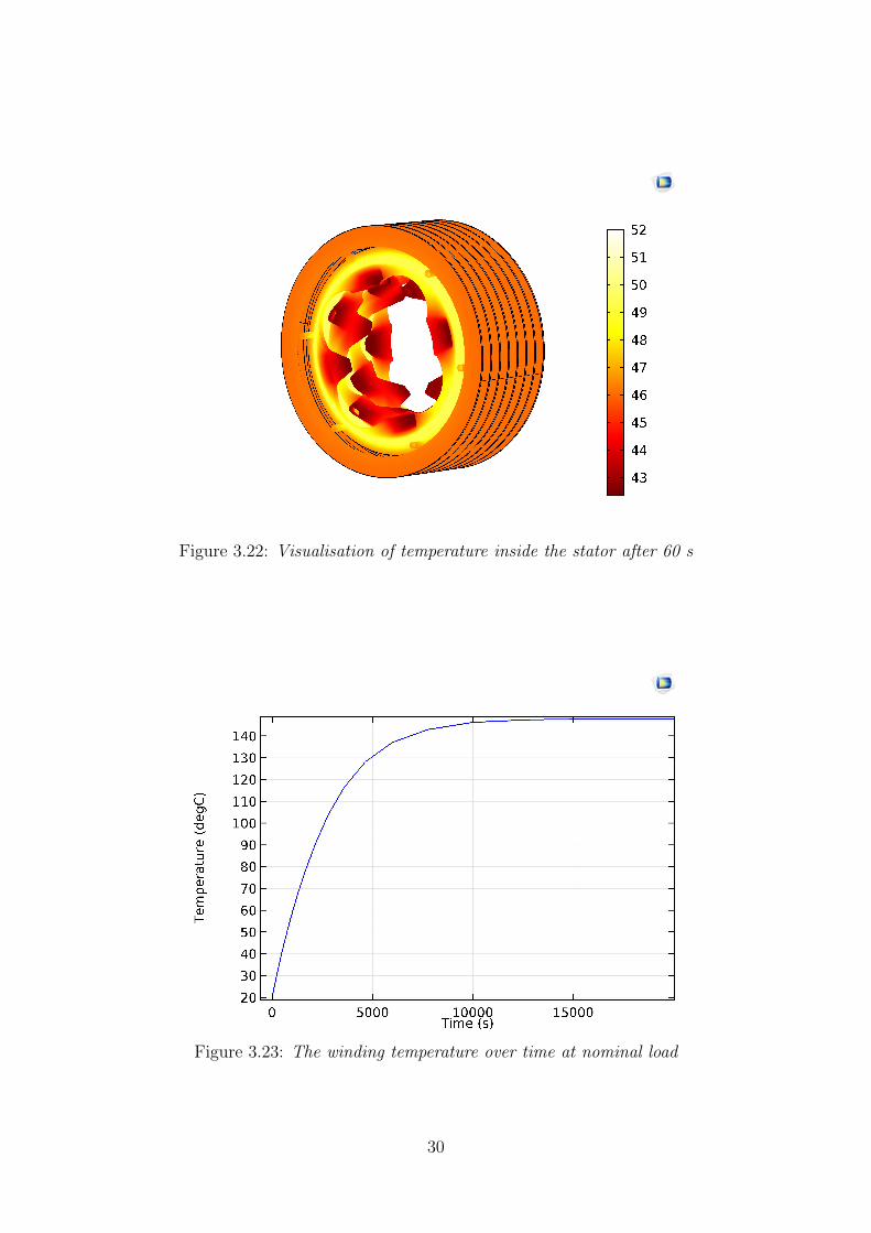
Figure 3.22: Visualisation of temperature inside the stator after 60 s

Figure 3.23: The winding temperature over time at nominal load

30

Figure 3.24: The winding temperature over time at peak torque

31

4 Prototyping

The active machine and sides of the housing is machined using an 3-axis CNC mill. Thematerial used for the active machine is Somaloy prototyping material. The datasheet can beseen in Appendix. Since the material is a sintered soft magnetic material, the machining of thematerial is relatively complex, because of chapping at edges.

4.1 Rotor

The fastening of the rotor was done using a jig, were the rotor was screwed down against thejig. The jig with a bolted rotor piece can be seen in Figure 4.1 and the threaded holes can beseen in Figure 4.2. The jig was also used to give the rotor some extra stability at the bottom,which was important to minimise the chapped edges. The resulting chapped edges can be seenin Figure 4.3. To minimise chapped edges sharp milling tools were needed, therefore millingtools for aluminium were used. A degradation of the milling tools were seen by a rapid increaseof chapping. So the milling tools needed to be changed between every other part.

Figure 4.1: Rotor jig with an mounted rotor part in the mill

32

Figure 4.2: Rotor segments with jig mounting holes

Figure 4.3: Chapped edges on final rotor parts

33

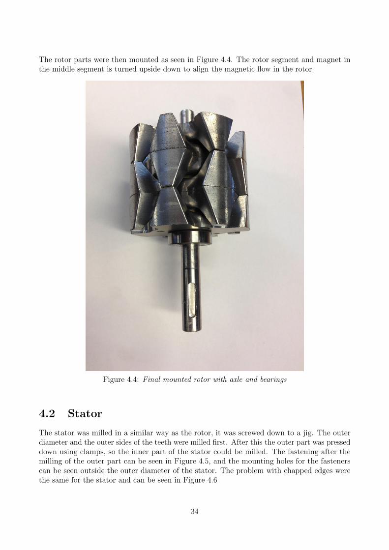
The rotor parts were then mounted as seen in Figure 4.4. The rotor segment and magnet inthe middle segment is turned upside down to align the magnetic flow in the rotor.

Figure 4.4: Final mounted rotor with axle and bearings

4.2 Stator

The stator was milled in a similar way as the rotor, it was screwed down to a jig. The outerdiameter and the outer sides of the teeth were milled first. After this the outer part was presseddown using clamps, so the inner part of the stator could be milled. The fastening after themilling of the outer part can be seen in Figure 4.5, and the mounting holes for the fastenerscan be seen outside the outer diameter of the stator. The problem with chapped edges werethe same for the stator and can be seen in Figure 4.6

34

Figure 4.5: Stator jig with an mounted stator part in the mill

Figure 4.6: Chapped edges on one of the final stator parts

35

4.3 Assembly

To be able to hold it all together two end plates were milled and the final parts can be seen inFigure 4.7

Figure 4.7: The sides to hold the machine together with bearing mounts

The windings for the machine were done by utilising a jig. A lathe was used to wind up thewindings on the jig with the correct dimensions, to easily fit into the stator segments. Thewinding jig setup can be seen in Figure 4.8.

The cooling mantle was turned and can be seen in Figure 4.9 mounted together with thestator. The final assembly of the stator can be seen in Figure 4.10. Thermal switches and atemperature sensor have been mounted on the windings for protective purposes.

36

Figure 4.8: Jig used to produce the windings

Figure 4.9: Assembly of the complete stator with cooling mantle

37

Figure 4.10: Inside of the winded stator, where the the thermal switches can be seen as white/bluecomponent taped to the winding

38

5 Measurements on prototype machine

The phase resistance was measured to 74.8 mΩ. The average self-inductance was 195 μH, thevarying inductance was measured to be 102 μH and the mutual inductance between phases wasmeasured and approximated to 48 μH. Ψm was measured to 0.021 V/Hz. These parameterswere then transformed over to the dq-domain using the method explained in section 2.1 andthe resulting values can be seen in Table 5.1.

Table 5.1: measured value in the dq-domain

Rs 74.8 mΩLsd 348 μHLsq 42 μHΨm 0.021 V/Hz

Since the equivalent parameters have been measured, the dq-voltages and dq-currents can becalculated in the same way as with the simulated values, using (2.19). By setting the maximumabsolute voltage to 48 V and the current angle equal to the MTPA angle shown in Figure 5.1.

d-Current [A]-150 -100 -50 0 50 100 150

q-C

urre

nt [A

]

0

20

40

60

80

100

120Constant currentConstant torqueMaximum torque per ampere

Figure 5.1: Visualisation of the field enhancement curve for maximum torque per ampere

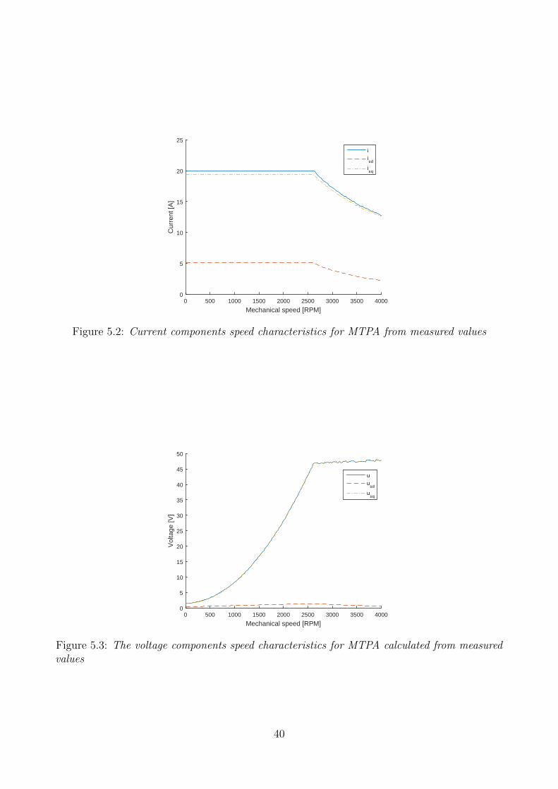
5.1 Nominal torque

For the measured nominal torque the nominal current is 20 A and the current speed character-isics can be seen in Figure 5.2, where the dq-components contributions is calculated using theMTPA angle from Figure 5.1. The voltage speed characteristics with dq-components can beseen in Figure 5.3 and the absolute voltage and current are plotted agains speed together inFigure 5.4.

39


Cur

rent

[A]

0

5

10

15

20

25

iisd

isq

Figure 5.2: Current components speed characteristics for MTPA from measured values


Vol

tage

[V]

0

5

10

15

20

25

30

35

40

45

50

uu

sd

usq

Figure 5.3: The voltage components speed characteristics for MTPA calculated from measuredvalues

40


Vol

tage

[V],

Cur

rent

[A]

0

5

10

15

20

25

30

35

40

45

50

ui

Figure 5.4: Voltage and current per speed characteristics calculated from measured values

41

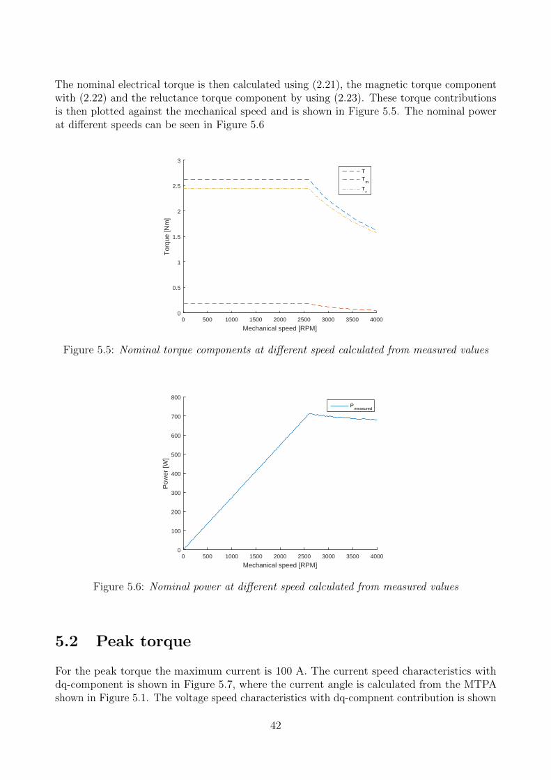
The nominal electrical torque is then calculated using (2.21), the magnetic torque componentwith (2.22) and the reluctance torque component by using (2.23). These torque contributionsis then plotted against the mechanical speed and is shown in Figure 5.5. The nominal powerat different speeds can be seen in Figure 5.6


Tor

que

[Nm

]

0

0.5

1

1.5

2

2.5

3

TT

m

Tr

Figure 5.5: Nominal torque components at different speed calculated from measured values


Pow

er [W

]

0

100

200

300

400

500

600

700

800P

measured

Figure 5.6: Nominal power at different speed calculated from measured values

5.2 Peak torque

For the peak torque the maximum current is 100 A. The current speed characteristics withdq-component is shown in Figure 5.7, where the current angle is calculated from the MTPAshown in Figure 5.1. The voltage speed characteristics with dq-compnent contribution is shown

42

in Figure 5.8. The absolute voltage and current is then plotted against speed in Figure 5.9


Cur

rent

[A]

0

10

20

30

40

50

60

70

80

90

100

110

iisd

isq

Figure 5.7: Maximum current components speed characteristics for MTPA from measuredvalues


Vol

tage

[V]

0

5

10

15

20

25

30

35

40

45

50

uu

sd

usq

Figure 5.8: The voltage components speed characteristics for MTPA calculated from measuredvalues

The electrical torque is then calculated using (2.21), the magnetic torque component with(2.22) and the reluctance torque component by using (2.23). These torque contributions isthen plotted against the mechanical speed and is shown in Figure 5.10. The maximum powerat different speeds can be seen in Figure 5.11

43


Vol

tage

[V],

Cur

rent

[A]

0

10

20

30

40

50

60

70

80

90

100

110

ui

Figure 5.9: Voltage and current per speed characteristics calculated from measured values


Tor

que

[Nm

]

0

2

4

6

8

10

12

14

16

18

20

TT

m

Tr

Figure 5.10: Maximum torque components at different speed calculated from measured values

44


Pow

er [W

]

0

200

400

600

800

1000

1200

1400

Pmeasured

Figure 5.11: Maximum power at different speed calculated from measured values

45

6 Analysis

In this section the comparison between the FE-calculated parameters and the measuredparameters is done. The FE-calculated and the measured parameter values are shown inTable 6.1. The FE-calculated winding resistance was calculated on the active part of thecoil winding, while the measured winding resistance was measured at the end terminal of thewinding. Both the FE-calculation and the measurements was done at room temperature. Theamount of extra length of the wire in the winding is approximated to be around 30 mm perphase which corresponds to approximately 4.5 mΩ. The difference in the dq-inductances comesfrom a difference of around 5% at the average self-inductance and the varying inductance, andthat the FE-calculated mutual inductance was approximated to 0.

Table 6.1: FE-calculated and measured value in the dq-domain

FE-calculated value measured valueLaverage 207.5 μH 195 μHLvarying 97.5 μH 102 μHLmutual 0 μH 48 μHRs 62.5 mΩ 74.8 mΩLsd 354 μH 348 μHLsq 61 μH 42 μHΨm 0.0206 V/Hz 0.021 V/Hz

The phase angle for MTPA is the same for both the FE-calculated and the measured values,this can be seen in Figure 6.1 where the MTPA lines overlay each other.

d-Current [A]-150 -100 -50 0 50 100 150

q-C

urre

nt [A

]

0

20

40

60

80

100

120 Constant currentConstant torqueMaximum torque per ampere

Figure 6.1: Visualisation of the field enhancement curve for maximum torque per ampere forFE-calculated and measured cases 46

6.1 Nominal torque

Comparison with the applied voltage at different speeds for nominal load torque can be seenin Figure 6.2. The difference between the FE-calculated and the measured torque speedcharacteristics is shown in Figure 6.3. It can be seen that the measured case have a highertorque, this seems to be from that the difference between Lsd and Lsq and that Ψm is largerin the measured case. The measured and FE-calculated power speed curves can be seen inFigure 6.4.


Vol

tage

[V]

0

5

10

15

20

25

30

35

40

45

50

umeasured

uFE-calculated

Figure 6.2: Comparison between the FE-calculated and the measured voltage speed characteristics


Tor

que

[Nm

]

0

0.5

1

1.5

2

2.5

3T

measured

TFE-calculated

Figure 6.3: Comparison between the FE-calculated and the measured maximum torque speedcharacteristics

47


Pow

er [W

]

0

100

200

300

400

500

600

700

800

Pmeasured

PFE-calculated

Figure 6.4: Comparison between the FE-calculated and the measured maximum power speedcharacteristics

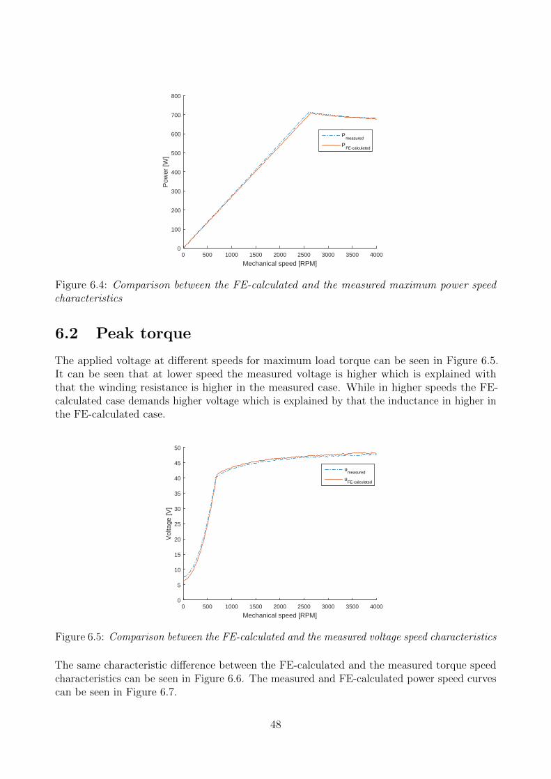
6.2 Peak torque

The applied voltage at different speeds for maximum load torque can be seen in Figure 6.5.It can be seen that at lower speed the measured voltage is higher which is explained withthat the winding resistance is higher in the measured case. While in higher speeds the FE-calculated case demands higher voltage which is explained by that the inductance in higher inthe FE-calculated case.


Vol

tage

[V]

0

5

10

15

20

25

30

35

40

45

50

umeasured

uFE-calculated

Figure 6.5: Comparison between the FE-calculated and the measured voltage speed characteristics

The same characteristic difference between the FE-calculated and the measured torque speedcharacteristics can be seen in Figure 6.6. The measured and FE-calculated power speed curvescan be seen in Figure 6.7.

48


Tor

que

[Nm

]

0

2

4

6

8

10

12

14

16

18

20

Tmeasured

TFE-calculated

Figure 6.6: Comparison between the FE-calculated and the measured maximum torque speedcharacteristics


Pow

er [W

]

0

200

400

600

800

1000

1200

1400

Pmeasured

PFE-calculated

Figure 6.7: Comparison between the FE-calculated and the measured maximum power speedcharacteristics

49

7 Conclusion

A claw pole machine with a nominal power of 708 W and a peak power of 1300 W with apeak torque of 19 Nm, has been designed, built and verified through measurements. Theequivalent circuit parameters was calculated to Rs = 62.5 mΩ, Lsd = 354 µH, Lsq = 61 µHand Ψm = 0.0206 while the measured equivalent parameters is Rs = 74.8 mΩ, Lsd = 348 µH,Lsq = 42 µH and Ψm = 0.021. The amount of hard magnetic material in the machine is 44 gand the reluctance torque in the machine was used as the primary generation of torque at nom-inal load. While at peak torque operation the magnetic torque contribution was significantlyhigher.

This work has shown that it is possible to prototype electrical machines using milling andturning using Somaloy Prototyping Material. Even if some difficulties exist, machining thematerial it is still a viable prototyping method. This could give small businesses a possibilityto design and prototype electrical machines without investing in specially built machinery andtooling otherwise necessary.

50

Bibliography

[1] J. Paul, “Investigating rare earth element mine development in epa region 8 and potentialenvironmental impacts.” EPA Document-908R11003, August 2011.

[2] E. Alonso, A. M. Sherman, T. J. Wallington, M. P. Everson, F. R. Field, R. Roth, and R. E.Kirchain, “Evaluating rare earth element availability: A case with revolutionary demandfrom clean technologies,” Environ Sci Technol., vol. 46, no. 8, pp. 4684–4684, 2012.

[3] Y. Suzhu, M. Zardinejad, J. Wei, W. Zhou, S. Subbiah, Z. Hongyu, P. Ji, Z. W. Xu, Fengzhou,H. Hocheng, H.-Y. Tsai, G. Yang, D. S. K. Wong, G. Qi, S. Z. Shanyong, B. Song, andM. K. Tiwari, Handbook of manufacturing engineering and technology. Springer, 2015.

[4] S. Lundmark, Application of 3-D Computation of Magnetic Fields to the Design of Claw-Pole Motors. Doktorsavhandlingar vid Chalmers tekniska hgskola. Ny serie, no: 2313,Institutionen for energi och milj, Elteknik, Chalmers tekniska hgskola,, 2005. 118.

[5] L. O. Hultman and A. G. Jack, “Soft magnetic composites-materials and applications,”Electric Machines and Drives Conference, vol. 1, pp. 516–522, 2003.

[6] H. Shokrollahi and K. Janghorban, “Soft magnetic composite materials (smcs),” Journalof Materials Processing Technology, vol. 189, no. 13, pp. 1 – 12, 2007.

[7] A. Balakrishnan, W. T. Joines, and T. G. Wilson, “Air-gap reluctance and inductance calcu-lations for magnetic circuits using a schwarz-christoffel transformation,” IEEE Transactionson Power electronics, vol. 12, p. 654 to 663, July 1997.

[8] E. N. H. Hembach, D. Gerling, “Analytical design of a claw-pole motor for electrical waterpump applications,”

51

Appendices

52

Quick and cheap with prototypingTooling is the preferred approach to manufacture

prototype components with Somaloy material.

Using this method, the prototyped component will

in all essential respects have the same properties

as a mass produced component.

A simplified approach is to machine the component

from a pre-fabricated blank. This can be a fast, low-

cost approach, but it also has the drawback that the

properties will in most cases be different from those

obtained by compaction. A special Somaloy Prototyping

Material with enhanced machinability has now been

developed in order to minimise these differences.

Somaloy Prototyping Material blanks exhibit stable

mechanical properties up to 150ºC.

For more information, please contact

your local sales representative.

www.hoganas.com/somaloy

Somaloy® Prototyping Material

To manufacture prototype components for soft

magnetic applications, the blanks should be machined

using conventional machining techniques (milling, turning,

drilling). Non conventional machining (such as electro

discharge machining, EDM) would deteriorate the material

and therefore should be avoided. Design with walls thinner

than 2 mm should be avoided.

In order to machine larger components, Somaloy

Prototyping Material blanks can be cut and glued

together (epoxy glue) before machining.

© H

ögan

äs A

B, S

epte

mb

er 2

014.

0

889H

OG

DRILLING• HSS self-centering drill

• Cutting speed: Vc = 30 m/min

• Feed speed: Vf = 60 mm/min

Here are some recommendations on tooling and process parameters for machining Somaloy® Prototyping Material.

MILLING• Super sharp carbide milling cutter,

for machining of aluminum and plastic materials

• Cutting speed: Vc in the range 100-125 m/min

• Feed per tooth: fz = 0.05 mm/tooth

TURNING• Cermet-polished sharp inserts,

for machining of aluminium and plastic materials

• Cutting speed: Vc in the range 50-300 m/min

• Feed: f = 0.12 mm/rev recommended for a good surface finish

• Cutting fluid can be used for better machinability

Somaloy Prototyping Material

Diameter 80 mmHeight 20 mm



Density [g/cc] 7.45 7.30 7.30

TRS @ ambient [MPa] 60 60 60

Resistivity [µΩ.m] 280 280 260

Bmax@4000 A/m [ T ] 1.26 1.19 1.23

Bmax@10000 A/m [ T ] 1.53 1.46 1.49

Hc [A/m] 200 200 210

µmax 455 430 435

Core losses @ 1T [W/kg]

50 Hz 5 5 5

200 Hz 21 22 22

400 Hz 46 48 49

600 Hz 74 79 79

800 Hz 104 111 111

1000 Hz 138 147 147

Typical Data and Machining Recommendations

All properties are measured on toroids (OD55 ID45 H5 mm) machined from the different Somaloy Prototyping Material blanks.

Home > Products > Permanent Magnets & Assemblies > Permanent Magnets> VACOMAX > VACOMAX 225 HR

VACOMAX 225 HRPermanent magnets with high remanence and the highest temperature stability attainable from rareearth materials. Use attemperatures up to 350 °C is possible (e.g. clutches).

Magnetic properties

Remanence Coercivity Energy density Temperaturecoefficient(RT 100 °C)

Temperaturecoefficient(RT 150 °C)

Brtyp.T

Brmin.T

HcBtyp.kA/m

HcBmin.kA/m

HcJmin.kA/m

(BH)maxtyp.kJ/m3

(BH)maxmin.kJ/m3

TC(Br)%/°C

TC(HcJ)%/°C

TC(Br)%/°C

TC(HcJ)%/°C

1.10 1.03 820 720 1590 225 190 0.030 0.18 0.035 0.19

Inner Magnetizing Field Strength

H mag min

kA/m kOe

3650 46

Characteristic physical properties at room temperature

Curietemperature

Specificelectricresistance

Specificheat

Thermalconductivity

Coefficient ofthermalexpansion20100 °C

Young'smodulus

Bendingstrength

Compressivestrength

Vickershardness

Stresscrackresistance

°C Ωmm2/m J/(kg⋅K) W (m⋅ K)

II c*) 106/K

⊥c*) 106/K kN/mm2 N/mm2 N/mm2 HV

KICN/mm3/2

800850 0.650.95 300500 515 812 1014 140170 80150 400900 550750 3060

*) II c: parallel to preferred magnetic direction ⊥ c: perpendicular to preferred magnetic direction

Typical demagnetization curves B(H) and J(H) at different temperatures

CONTACT

Do you have general questions about our products?We would be pleased to assist you!

Email

Contact form

Typical irreversible losses at different working points as a function of temperature

designing and prototyping of a transverse flux machine in...

Documents