designing an interplanetary autonomous …oaktrust.library.tamu.edu/.../karimi-dissertation.pdf ·...
TRANSCRIPT

DESIGNING AN INTERPLANETARY AUTONOMOUS
SPACECRAFT NAVIGATION SYSTEM USING VISIBLE PLANETS
A Dissertation
by
REZA RAYMOND KARIMI
Submitted to the Office of Graduate Studies ofTexas A&M University
in partial fulfillment of the requirements for the degree of
DOCTOR OF PHILOSOPHY
May 2012
Major Subject: Aerospace Engineering

DESIGNING AN INTERPLANETARY AUTONOMOUS
SPACECRAFT NAVIGATION SYSTEM USING VISIBLE PLANETS
A Dissertation
by
REZA RAYMOND KARIMI
Submitted to the Office of Graduate Studies ofTexas A&M University
in partial fulfillment of the requirements for the degree of
DOCTOR OF PHILOSOPHY
Approved by:
Chair of Committee, Daniele MortariCommittee Members, John L. Junkins
Srinivas Rao VadaliJohnny E. HurtadoShankar Bhattacharya
Head of Department, Dimitris Lagoudas
May 2012
Major Subject: Aerospace Engineering
iii
ABSTRACT
Designing an Interplanetary Autonomous
Spacecraft Navigation System Using Visible Planets. (May 2012)
Reza Raymond Karimi, B.S., Tehran Azad University;
M.S., Tarbiat Modares University
Chair of Advisory Committee: Dr. Daniele Mortari
A perfect duality exists between the problem of space-based orbit determina-
tion from line-of-sight measurements and the problem of designing an interplanetary
autonomous navigation system. Mathematically, these two problems are equivalent.
Any method solving the first problem can be used to solve the second one and, vice
versa. While the first problem estimates the observed unknown object orbit using
the known observer orbit, the second problem does exactly the opposite (e.g. the
spacecraft observes a known visible planet). However, in an interplanetary naviga-
tion problem, in addition to the measurement noise, the following “perturbations”
must be considered: 1) light-time effect due to the finite speed of light and large
distances between the observer and planets, and 2) light aberration including special
relativistic effect. These two effects require corrections of the initial orbit estimation
problems. Because of the duality problem of space-based orbit determination, several
new techniques of angles-only Initial Orbit Determination (IOD) are here developed
which are capable of using multiple observations and provide higher orbit estima-
tion accuracy and also they are not suffering from some of the limitations associated
with the classical and some newly developed methods of initial orbit determination.
Using multiple observations make these techniques suitable for the coplanar orbit
determination problems which is the case for the spacecraft navigation using visible
planets as the solar system planets are all almost coplanar. Four new IOD techniques
iv
were developed and Laplace method was modified. For the autonomous navigation
purpose, Extended Kalman Filter (EKF) is employed. The output of the IOD al-
gorithm is then used as the initial condition to extended Kalman filter. The two
“perturbations” caused by light-time effect and stellar aberration including special
relativistic effect also need to be taken into consideration and corrections should be
implemented into the extended Kalman filter scheme for the autonomous spacecraft
navigation problem.

v
To my parents

vi
To Issac Newton

vii
ACKNOWLEDGMENTS
I would like to thank my research advisor, Dr. Daniele Mortari, and my teaching
supervisor, Mr. Michael Golla, for being great mentors and friends. I would like to
thank Dr. John L. Junkins, Dr. S. Rao Vadali, Dr. Johny E. Hurtado, Dr. Shankar
Bhattacharyya, Dr. James Turner, and Dr. Walter Haisler for their help and support.
Also I would like to thank my dear friend Johnathan Hebert and his father for their
unconditional support.

viii
TABLE OF CONTENTS
CHAPTER Page
I INTRODUCTION . . . . . . . . . . . . . . . . . . . . . . . . . . 1
A. Orbital Dynamics Background . . . . . . . . . . . . . . . . 1
B. Duality Between a Space-Based Orbit Determination
Problem and Interplanetary Spacecraft Navigation . . . . . 4
C. Survey on Initial Orbit Determination Methods . . . . . . 5
1. Laplace . . . . . . . . . . . . . . . . . . . . . . . . . . 7
2. Gauss . . . . . . . . . . . . . . . . . . . . . . . . . . . 8
3. Gibbs . . . . . . . . . . . . . . . . . . . . . . . . . . . 9
4. Herrick-Gibbs . . . . . . . . . . . . . . . . . . . . . . 11
5. Double r-iteration . . . . . . . . . . . . . . . . . . . . 12
6. Gooding . . . . . . . . . . . . . . . . . . . . . . . . . 15
7. Other IOD Methods . . . . . . . . . . . . . . . . . . . 17
8. Proposed IOD Algorithms . . . . . . . . . . . . . . . . 17
D. Result Presentation . . . . . . . . . . . . . . . . . . . . . . 18
1. Orbit Error . . . . . . . . . . . . . . . . . . . . . . . . 19
E. Noise Simulation . . . . . . . . . . . . . . . . . . . . . . . 20
II MODIFIED LAPLACE INITIAL ORBIT DETERMINA-
TION METHOD . . . . . . . . . . . . . . . . . . . . . . . . . . 22
A. Introduction . . . . . . . . . . . . . . . . . . . . . . . . . . 22
B. Laplace Original Method . . . . . . . . . . . . . . . . . . . 24
C. Modifications . . . . . . . . . . . . . . . . . . . . . . . . . 24
D. Selected Test Scenarios and Results . . . . . . . . . . . . . 29
1. Non-coplanar Scenarios . . . . . . . . . . . . . . . . . 29
2. Coplanar Scenarios . . . . . . . . . . . . . . . . . . . . 31
E. Conclusion . . . . . . . . . . . . . . . . . . . . . . . . . . . 33
III INITIAL ORBIT DETERMINATION USING MULTIPLE
OBSERVATIONS . . . . . . . . . . . . . . . . . . . . . . . . . . 35
A. Introduction . . . . . . . . . . . . . . . . . . . . . . . . . . 35
B. Formulation Development . . . . . . . . . . . . . . . . . . 37
1. Numerical Solution . . . . . . . . . . . . . . . . . . . . 38
2. Extension to Multiple Observations . . . . . . . . . . 41
ix
CHAPTER Page
3. Least-Squares Solution . . . . . . . . . . . . . . . . . . 42
4. Gauss-exact . . . . . . . . . . . . . . . . . . . . . . . . 43
C. Simulations and Results . . . . . . . . . . . . . . . . . . . 44
1. Sensitivity Analysis . . . . . . . . . . . . . . . . . . . 50
2. Results Bias . . . . . . . . . . . . . . . . . . . . . . . 55
D. Conclusions . . . . . . . . . . . . . . . . . . . . . . . . . . 57
IV INITIAL ORBIT DETERMINATION USING PRESCRIBED
ORBITS . . . . . . . . . . . . . . . . . . . . . . . . . . . . . . . 59
A. Introduction . . . . . . . . . . . . . . . . . . . . . . . . . . 59
B. Algorithm Development . . . . . . . . . . . . . . . . . . . 60
C. Example Problems and Results . . . . . . . . . . . . . . . 63
D. Conclusion . . . . . . . . . . . . . . . . . . . . . . . . . . . 72
V INITIAL ORBIT DETERMINATION BASED ON VARIA-
TION OF ORBITAL ERROR . . . . . . . . . . . . . . . . . . . 73
A. Introduction . . . . . . . . . . . . . . . . . . . . . . . . . . 73
B. Methodology . . . . . . . . . . . . . . . . . . . . . . . . . 74
1. Orbit Error . . . . . . . . . . . . . . . . . . . . . . . . 74
a. Residuals Based on Orbit Orientation Error. . . . 77
b. Residuals Based on Orbit Shape Error . . . . . . 79
C. Generalizing to Multiple Observations . . . . . . . . . . . . 81
D. Selected Test Scenarios and Results . . . . . . . . . . . . . 83
E. Conclusions . . . . . . . . . . . . . . . . . . . . . . . . . . 87
VI SPACE-BASED INITIAL ORBIT DETERMINATION . . . . . 89
A. Challenges of Space-based IOD versus Ground-based IOD . 89
1. Satellite Conjunction . . . . . . . . . . . . . . . . . . 89
2. Problem Description . . . . . . . . . . . . . . . . . . . 90
3. Noise Effect Reduction . . . . . . . . . . . . . . . . . 92
4. Simulation and Results . . . . . . . . . . . . . . . . . 93
a. LEO-to-LEO (Iridium 33-Cosmos 2251 Scenario) 94
b. LEO-to-GEO (Coplanar) . . . . . . . . . . . . . . 96
c. GEO-to-GEO . . . . . . . . . . . . . . . . . . . . 98
5. Conclusion . . . . . . . . . . . . . . . . . . . . . . . . 98
VII DESIGNING AN INTERPLANETARY AUTONOMOUS SPACE-
CRAFT NAVIGATION SYSTEM USING VISIBLE PLANETS 102

x
CHAPTER Page
A. Challenges of an Interplanetary Spacecraft Navigation
Problem . . . . . . . . . . . . . . . . . . . . . . . . . . . . 102
a. Light-time Correction . . . . . . . . . . . . . . . . 103
b. Stellar Aberration Including Restricted (Spe-
cial) Relativistic Effect . . . . . . . . . . . . . . . 104
B. Extended Kalman Filter Implementation . . . . . . . . . . 107
C. Results . . . . . . . . . . . . . . . . . . . . . . . . . . . . . 113
D. Conclusion . . . . . . . . . . . . . . . . . . . . . . . . . . . 117
VIII CONCLUSION . . . . . . . . . . . . . . . . . . . . . . . . . . . 118
IX FUTURE WORK . . . . . . . . . . . . . . . . . . . . . . . . . . 120
REFERENCES . . . . . . . . . . . . . . . . . . . . . . . . . . . . . . . . . . . 121
APPENDIX A . . . . . . . . . . . . . . . . . . . . . . . . . . . . . . . . . . . 126
VITA . . . . . . . . . . . . . . . . . . . . . . . . . . . . . . . . . . . . . . . . 127

xi
LIST OF TABLES
TABLE Page
I Pseudo-code for Gooding Algorithm . . . . . . . . . . . . . . . . . . 16
II Non-Coplanar Monte Carlo Analysis for 2326 LEO Scenarios
(3σ = 10” and ∆t = 10s) . . . . . . . . . . . . . . . . . . . . . . . . . 30
III Orbital Elements for a Single Random Scenario: Non-coplanar . . . . 30
IV Performance Comparison of Original and Modified Laplace for
One Single Non-coplanar Scenario (3σ = 10” and ∆t = 10s) . . . . . 31
V Coplanar Monte Carlo Analysis for 2212 LEO Scenarios (3σ =
10” and ∆t = 10s) . . . . . . . . . . . . . . . . . . . . . . . . . . . . 32
VI Orbital Elements for a Single Random Scenario: Coplanar . . . . . . 32
VII Performance Comparison of the Modified Laplace for One Single
Coplanar Scenario (3σ = 10” and ∆t = 10s) . . . . . . . . . . . . . . 32
VIII Tracking Equatorial LEO Satellite (Coplanar Case) . . . . . . . . . . 47
IX Tracking a 45 deg. LEO Satellite (Inclined Case) . . . . . . . . . . . 48
X Tracking a Polar LEO Satellite (Orthogonal Case) . . . . . . . . . . 49
XI Tracking an Asteroid on Hyperbolic Orbit . . . . . . . . . . . . . . . 50
XII Orbital Elements . . . . . . . . . . . . . . . . . . . . . . . . . . . . . 51
XIII Initial Real Position and Velocity Vectors . . . . . . . . . . . . . . . 51
XIV Monte Carlo Analysis for 441 Non-coplanar LEO Scenarios (3σ =
10′′), aerror < 0.25%, berror < 0.25%, and δ < 0.05 . . . . . . . . . 84
XV Monte Carlo Analysis for 438 Coplanar LEO Scenarios (3σ =
10′′), aerror < 0.5%, berror < 0.5%, and θ < 0.05 . . . . . . . . . . 84

xii
TABLE Page
XVI Orbital Elements for a Single Random Scenario . . . . . . . . . . . . 85
XVII Performance Comparison for One Non-coplanar Single Scenario
(3σ = 10′′), ∆t = 60 s . . . . . . . . . . . . . . . . . . . . . . . . . . 86
XVIII Performance Comparison for One Non-coplanar Single Scenario
(3σ = 10′′), ∆t = 80s . . . . . . . . . . . . . . . . . . . . . . . . . . . 86
XIX Performance Comparison for One Non-coplanar Single Scenario
(3σ = 10′′), ∆t = 100 s . . . . . . . . . . . . . . . . . . . . . . . . . . 87
XX Performance Comparison for One Coplanar Single Scenario (3σ =
10′′), ∆t = 150 s . . . . . . . . . . . . . . . . . . . . . . . . . . . . . 87
XXI Performance Comparison for One Coplanar Single Scenario (3σ =
10′′), ∆t = 180 s . . . . . . . . . . . . . . . . . . . . . . . . . . . . . 88
XXII Orbital Elements of Satellites for Simulation . . . . . . . . . . . . . . 95
XXIII Iridium33 - Cosmos2251 Scenario Using Jn, Nobs = 10, ∆t = 20s,
3σ = 10” . . . . . . . . . . . . . . . . . . . . . . . . . . . . . . . . . 97
XXIV Iridium33 - Cosmos2251 Scenario Using Jn, Nobs = 10, ∆t = 40s,
3σ = 10” . . . . . . . . . . . . . . . . . . . . . . . . . . . . . . . . . 97
XXV Iridium33 - Cosmos2251 Scenario Using Jn, Nobs = 10, ∆t = 60s,
3σ = 10” . . . . . . . . . . . . . . . . . . . . . . . . . . . . . . . . . 98
XXVI Iridium33 - Cosmos2251 Scenario Using Pn, Nobs = 8, ∆t = 80s,
3σ = 10” . . . . . . . . . . . . . . . . . . . . . . . . . . . . . . . . . 98
XXVII Iridium33 - Cosmos2251 Scenario Using Pn, Nobs = 8, ∆t = 100s,
3σ = 10” . . . . . . . . . . . . . . . . . . . . . . . . . . . . . . . . . 99
XXVIII Orbital Elements of LEO-GEO Scenario (Circular and Coplanar
Orbits) . . . . . . . . . . . . . . . . . . . . . . . . . . . . . . . . . . 99
XXIX LEO-to-GEO Scenario, (Circular and Coplanar), Nobs = 8, ∆t =
900s, 3σ = 10” . . . . . . . . . . . . . . . . . . . . . . . . . . . . . . 100
XXX LEO-to-GEO Scenario, (Circular and Coplanar), Nobs = 8, ∆t =
1200s, 3σ = 10” . . . . . . . . . . . . . . . . . . . . . . . . . . . . . . 100

xiii
TABLE Page
XXXI LEO-to-GEO Scenario, (Circular and Coplanar), Nobs = 8, ∆t =
1800s, 3σ = 10” . . . . . . . . . . . . . . . . . . . . . . . . . . . . . . 101
XXXII Continuous-discrete Extended Kalman Filter . . . . . . . . . . . . . . 109

xiv
LIST OF FIGURES
FIGURE Page
1 Scenario II:Relative Position Percentage Error vs. Noise (4t =
50 s) . . . . . . . . . . . . . . . . . . . . . . . . . . . . . . . . . . . . 52
2 Scenario II:Relative Position Percentage Error vs. Time Interval
4t (σ = 5′′) . . . . . . . . . . . . . . . . . . . . . . . . . . . . . . . . 53
3 Scenario II:Performance of Ln vs Double r-iteration and Gauss-
exact vs. Time Interval 4t (σ = 5′′) . . . . . . . . . . . . . . . . . . 54
4 Scenario II: Relative Position Percentage Error Sensitivity to Or-
bital Elements. Top: Eccentricity, Middle: Semi-major Axis,
Bottom: True Anomaly. (Ω = 345, ω = 15, i = 45), (∆t = 50
s, using Jn) . . . . . . . . . . . . . . . . . . . . . . . . . . . . . . . . 55
5 Scenario II: Relative Position Percentage Error of Different Ob-
servations Combinations vs. Interval 4t (σ = 5′′) . . . . . . . . . . . 56
6 Error Histogram of J3 . . . . . . . . . . . . . . . . . . . . . . . . . . 57
7 Error Histogram of L3 . . . . . . . . . . . . . . . . . . . . . . . . . . 57
8 Orbit Shape and Orientation (Angular momentum) Error Using
P7, Scenarios=2182 . . . . . . . . . . . . . . . . . . . . . . . . . . . . 65
9 Orbit Shape and Orientation (Angular Momentum) Error Using
J7, Scenarios=2182 . . . . . . . . . . . . . . . . . . . . . . . . . . . . 65
10 Orbit Shape and Orientation (Angular Momentum) Error Using
L7, Scenarios=2182 . . . . . . . . . . . . . . . . . . . . . . . . . . . . 66
11 Orbit Shape and Orientation (Angular Momentum) Error Using
P7, Scenarios=2182 . . . . . . . . . . . . . . . . . . . . . . . . . . . . 66
12 Orbit Shape and Orientation (Angular Momentum) Error Using
J7, Scenarios=2182 . . . . . . . . . . . . . . . . . . . . . . . . . . . 67

xv
FIGURE Page
13 Orbit Shape and Orientation (Angular Momentum) Error Using
L7,Scenarios=2182 . . . . . . . . . . . . . . . . . . . . . . . . . . . . 67
14 Orbit Shape and Attitude Error Using P7, Scenarios=2147 out of 2336 69
15 Orbit Shape and Attitude Error Using L7, Scenarios=2214 out of 2336 69
16 Orbit Shape and Attitude Error Using Gauss Method, Scenar-
ios=1974 out of 2336 . . . . . . . . . . . . . . . . . . . . . . . . . . . 70
17 Orbit Shape and Attitude Error Using P7, Scenarios=2201 out of 2336 70
18 Orbit Shape and Attitude Error Using L7, Scenarios=1939 out of 2336 71
19 Orbit Shape and Attitude Error Using Gauss Method, Scenar-
ios=1813 out of 2336 . . . . . . . . . . . . . . . . . . . . . . . . . . . 71
20 Orbit Error Definition as a Complex Number . . . . . . . . . . . . . 76
21 A Typical Potential Collision Problem . . . . . . . . . . . . . . . . . 91
22 Measured Directions: True, Noisy, and Filtered . . . . . . . . . . . . 94
23 Orbits of the Simulated Spacecrafts . . . . . . . . . . . . . . . . . . . 96
24 Light Aberration Caused by the Finite Speed of Light . . . . . . . . 106
25 Light-time and Stellar Aberration Including Restricted Relativis-
tic Effect Correction to the IOD Algorithm . . . . . . . . . . . . . . 107
26 Azimuth and Elevation Angles as Input Measurements . . . . . . . . 111
27 Light-time and Stellar Aberration Including Restricted Relativis-
tic Effect Correction to EKF . . . . . . . . . . . . . . . . . . . . . . 112
28 Estimated Position and Velocity Error with the 3-σ Bounds . . . . . 115
29 Estimated and True Position and Velocity Components . . . . . . . . 116

1
CHAPTER I
INTRODUCTION
In the first section of this chapter, a short review of the history of orbital dynamics
is presented. In the second section, the duality between space-based orbit deter-
mination problem and interplanetary spacecraft navigation is explained followed by
a survey and review of the classical and some modern angles-only initial orbit de-
termination methods. Then, several Initial Orbit Determination (IOD) techniques
developed are introduced and at the end of this chapter, two different ways of pre-
senting the results will be described.
A. Orbital Dynamics Background
The ancient Greeks were best known for their contribution to mathematics. Euclid
(330-370 B.C.) is credited with being the first to write about conic sections, but his
writings were lost. Consequently, Apollonius (287-212 B.C) is credited with the first
known treatise on conic sections (225 B.C.) and was the first to name the sections.
He probably also introduced excentric and epicycle theories of orbital motions. Al-
though records from this period are scarce because of fires and destruction over the
time, it is commonly thought that that Aristarchus (310-250 B.C.) suggested the
Earth revolved around the Sun. Unfortunately, his theory did not gain immediate
acceptance because it could not predict the position of Mars and did not accommo-
date the expected angular separation from different viewing locations. It was almost
1800 years later when Copernicus used some of Aristarchus’ results to develop his
own heliocentric model. Eratosthenes (275-194 B.C.) was perhaps the first person
The journal model is AIAA Journal of Guidance, Control, and Dynamics.

2
to obtain a reasonable estimate of the Earth’s radius. He did this using knowledge
of the Sun’s light rays during the summer solstice in Syene, Egypt.
Hipparchus (161-126 B.C.) developed spherical geometry and taught the Earth
was the center of the universe (even though Pythagorous and Aristarchus placed the
Sun at the center much earlier). Hipparchus also noticed an increase in the longitude
of the stars, [1]. Hipparchus likewise developed the first system of cataloging star
magnitudes. The list categorized about 1,000 stars by brightness. Hipparchus also
developed theories to describe orbital motion. He made very accurate observations,
which presented some problems when trying to describe the orbital motion. Lastly,
Claudisu Ptolemaeus (usually called Ptolemy) (100-170 A.D.) published a 13-volume
work, called the Mathematical Collection or the Almagest, which contained his theory
of an Earth-centered solar system. He used the results of Hipparchus but was unaware
of earlier astronomers’ works that declared the Earth was spherical and rotating
around the Sun.
The long period of inactivity in the roots of orbital dynamics from the end of
ancient times began to change with Nicholas Copernicus (1473-1543). Copernicus
was the first scientist to bridge the gap between antiquity and modern times. He
worked more than 31 years to resolve the fundamental motions of the solar system,
[2]. In many respects, Galileo Galilei (1564-1642) picked up where Copernicus left
off. In fact, he adopted the Copernicus’ ideas a few years before 1597, even though
his famous works were published more than ten years later. The main advantage of
his research was his use of the telescope for regular and dedicated scientific research.
Galileo’s perhaps best known for his support of theories which opposed the religious
doctrine of the time. Galileo Galilei served a valuable role in continuing the new
thought which was about to take solid shape under Tycho Brahe, Johann Kepler,
and Isaac Newton. Scientific change accelerated when Johann Kepler (1571-1630)

3
an Tycho Brahe (1546-1601) combined forces. In 1594, Kepler accepted a teaching
position in Graz. Part of his duties in this position was to compile annual almanacs.
Several years and many positions later, Kepler became the imperial court mathe-
matician for Emperor Rudolf II in Prague in 1601. Tycho Brahe had died shortly
before, leaving Kepler with all his very precious observational data. This was perfect
for Kepler. Unfortunately, providing horoscope for the Emperor was not thrilling
work, but it provided income and allowed him to pursue technical interests on the
side.
The relatively “large” eccentricity of the Martian orbit attracted Kepler’s inter-
est. After many years of work, he published Astronomia Nova (New Astronomy) in
1609. This was a huge work containing his first two laws. It is worth mentioning that
Kepler completed the paper in 1605 but couldn’t print it for four more years. Fi-
nally, Kepler published his third law in 1619 as Harmonics Mundi Libri V (Harmony
of the World). Kepler’s third law now receives particular attention in the literature,
but all three are important; 1) The orbit of each planet is an ellipse with the Sun at
one focus, 2) The line joining the planet to the Sun sweeps out equal areas in equal
times, and 3) The square of the period of a planet is proportional to the cube of its
mean distance to the Sun.
As remarkable as Kepler’s laws were, they did not completely solve planetary mo-
tion. They captured the kinematics of motion, but the dynamics of motion remained
unsolved until Sir Isaac Newton (1642-1727) unlocked them. Newton published his
famous three laws in 1687 (Emmond Halley (1656-1742), the discoverer of Hally’s
Comet, paid for the printing of the manuscript) as Philosophia Naturalis Principa Mathematica
or Principa. Newton was fascinated by the beauty and precision of Kepler’s laws and
set about the task of discovering what force law must be existing between bodies in
the solar system to be consistent with his laws of motion and Kepler’s experimentally
4
verified laws of planetary motion. From this analysis, Newton discovered the law of
universal gravitation, and the analytical solution of Keplerian motion, [3].
B. Duality Between a Space-Based Orbit Determination Problem and Interplane-
tary Spacecraft Navigation
A perfect Duality (actually an equivalency) exists between the problem of space-
based orbit determination from line-of-sight measurements and the problem of de-
signing an interplanetary autonomous navigation system. Mathematically, these two
problems are equivalent. Any method solving the first problem can be used to solve
the second and, viceversa. While the first problem estimates the observed unknown
object orbit using the known observer orbit, the second problem does exactly the
opposite (e.g. the spacecraft observes a known visible planet). However, in an inter-
planetary navigation problem, in addition to the measurement noise, the following
“perturbations” must be considered: 1) the light-time effect due to the finite speed
of light and large distances between the observer and planets. This effect causes the
measured lines-of-sight at time t = t0 (spacecraft time) belong to the position of the
observed planet at time t = t0 − δt where δt is the unknown time that takes light
to travel from the planet to the spacecraft, and 2) the restricted relativistic light
aberration effect. This effect causes the measured lines-of-sight to be compressed
towards the direction of the spacecraft velocity vector and the angle between the
measured line-of-sight and velocity vector seems smaller than the true angle. These
two effects require corrections of the initial orbit estimation problems.
In this work, several new techniques of angles-only initial orbit determination
were developed which are capable of using multiple observations resulting in higher
orbit estimation accuracy and also bypassing some of the drawbacks associated with

5
the classical and some newly developed IOD methods. In the following section, a
review of the angles-only initial orbit determination methods is presented.
C. Survey on Initial Orbit Determination Methods
Satellite Orbit Determination (OD) can be described as the method of determining
the position and velocity (i.e., the state vector, state, or ephemeris) of an orbiting
object such as an interplanetary spacecraft or an Earth orbiting satellite. The OD
problem is generally described by the computational process (generally solved by
applying statistical estimation techniques) of determining the state of a satellite as a
function of time using the set of measurements collected onboard the satellite and/or
by ground-based tracking stations.
The satellite is indeed influenced by a variety of external forces, including grav-
ity, atmospheric drag, solar radiation pressure, third-body perturbations, Earth tidal
effects, and general relativity in addition to satellite internal control actions. The
complex description of these forces results in a highly nonlinear set of dynamical
equations of motion. Furthermore, the lack of detailed knowledge of the physics of
the environment through which the satellite travels limits the accuracy with which
the state of the satellite can be determined at any given time. Similarly, observa-
tional data are inherently nonlinear with respect to the state of the satellite. The
impossibility to find closed form solutions of these nonlinear equations forces to use
linearization so that linear estimation techniques can be used to resolve the OD
problem. The solution can be obtained over a short orbit arc of less than 1 hr over a
long orbit arc approaching many days or longer. Different techniques have also been
devised to obtain an accurate solution. The key ideas of these techniques can be
applied to a wide variety of OD problems, ranging from near-Earth satellite orbits

6
to lunar and interplanetary transfer orbits.
As stated above, the state vector of an orbiting satellite is composed of a set
of position and velocity components that are usually defined in a inertial reference
frame, normally with origin at Earth’s center. The term “state vector” is sometimes
used interchangeably with the word “state” to describe the satellites location in 3-D
space.
The objective of Precise Orbit Determination (POD) is to obtain an accurate
orbit estimation that accounts for the dynamical environment in which the motion
occurs, including all relevant forces affecting the satellites motion. To initiate this
process, a preliminary orbit is estimated using a minimum number of observations.
This estimate provides the initial conditions for numerical integration of the nonlinear
differential equations of motion to obtain a reference orbit. A differential correction
procedure is then used to iteratively correct the reference orbit and refine the final
orbit solution. An improved orbit is thus obtained by using many observations
or observational data sets along with an accurate physics-based model describing
the dynamical environment. POD orbits are those that best satisfy all available
observations and require the ultimate in observational accuracy, [4].
Probably Hipparchus (190 B.C. − 120 B.C.) can be considered as the first one
who did work on orbit determination. He is known to have been a working astronomer
at least from 162 to 127 BC, [5]. Hipparchus is considered the greatest ancient as-
tronomical observer and, by some, the greatest overall astronomer of antiquity. He
was the first whose quantitative and accurate models for the motion of the Sun and
Moon survive. For this he certainly made use of the observations and perhaps the
mathematical techniques accumulated over centuries by the Chaldeans from Baby-
lonia. With his solar and lunar theories and his trigonometry, he may have been the
first to develop a reliable method to predict solar eclipses. In the modern ages, one

7
of the first works on the development of orbit determination methods were carried
out by Laplace [6] and Gauss [7], [8] about two centuries ago. Their techniques were
based upon three angles-only observations. Indeed the first attempts to develop the
orbit determination techniques were for the applications of comets,asteroids, planets,
and all other natural celestial bodies. The technique developed by the astronomer
Paul Herget [10], [11] in late 1930’s early 1940’s was capable of using multiple ob-
servations. With the advent of the Space age, more computer-based algorithms with
iterative nature were developed among which the Double-r iteration technique by
Escobal [12] and more recently a new approach by Gooding [13], which are both
angles-only methods, could be mentioned. In this the following, some classical and
rather newly developed angles-only initial orbit determination methods are briefly
reviewed.
1. Laplace
Laplace’s method of orbit determination was first proposed in the Memoires de
l’Academie Royal des Sciences de Paris in 1780 [6]. The method was originally
developed for planets and comets and yields poor results for near-earth orbiting ob-
jects. The algorithm uses a span of measured lines-of-sight vectors and estimates the
middle range (eventually satellite position vector) and velocity. The technique needs
at least three measured directions, but with more data available, the first and second
derivatives of the quantities involved in the algorithm can be approximated with a
higher accuracy. Laplace started with taking the fist and second derivatives of the
geometry of an orbit determination problem, r = R + ρ ρ, where r and R are the
unknown position vector of the observed orbiting object and known position vector
of the observer respectively

8
r = ρρ+ ρ ˙ρ+ R (1.1)
and
r = ρρ+ 2ρ ˙ρ+ ρ¨ρ+ R (1.2)
The first and second derivatives of the observer position vector R and measured
line-of-sight ρ are known, and the second derivative of the spacecraft position vector
r is replaced by the two-body Keplerian motion equation. The unknown range ρ and
its derivatives can be determined through the following set of equations
[ρ 2 ˙ρ ¨ρ+
µ
r3ρ
]3×3
ρ
ρ
ρ
3×1
= −
R +µ
r3R
3×1
(1.3)
For more details on Laplace’s method, see Chapter 2.
2. Gauss
The Gauss IOD method was developed by Carl Friedrich Gauss, a German math-
ematician, in 1809. The method has been developed based on lines-of-sight mea-
surements and requires three observations. Gauss’ method receives mixed reviews
from the astrodynamic community. The opinions range from little concern because
the method works best for interplanetary studies, to feeling that it is not very accu-
rate for near-Earth orbit determination. Long [9] suggests that it works best when
the angular separation between observation is less than 60. The method performs
remarkably well when the data is separated by 10 or less.
The success of Gauss’ method also depends on the method used to determine the

9
Lagrange f and g functions. In general, Guass’ algorithm is a rather robust technique
to determine a spacecraft position with angles-only measurements, [3]. The Gauss
method takes advantage of the fact that the orbit motion is planar and, therefore,
each position vector r can be expressed in terms of a linear combination of the other
position vectors as
a1r1 + a2r2 + a3r3 = 0 (1.4)
or
r2 = c2r1 + d2r3 (1.5)
and since all these three position vectors should satisfy the two-body Keplerian
motion, and also position vectors r1 and r3 can be related to r2 through f and
g functions, the coefficients c2 and d2 can be determined in terms of f and g. The
original Gauss’ method of initial orbit determination uses three lines of dight. The
detailed procedure of the technique will be discussed in Chapter 3.
Gauss’ method was refined by Gibbs in 1888, [14] and [15]. Gauss included
terms up to t2 in the expressions for f and g functions, while Gibbs showed how
to include terms up to t4. Moulton investigated the radius of convergence of the
involved series expansion in 1903, [16].
3. Gibbs
Gibbs method uses three position vectors to determine the orbit,[17]. Solving Gibbs
relies on knowing the Gauss formulation. Indeed, the first few steps are actually a
variant of the original Gauss method. The Gibbs problem is formed supposing we
know three non-zero coplanar position vectors which represent three time-sequential
10
vectors of a satellite in its orbit. These assumptions are needed for a solution.
The“non-zero” constraint simply prevents divided-by-zero operation. The sequential
requirement is very important because we consider a sequence of vectors while form-
ing the solution and take several cross products based on the given order. Changing
from a sequential order will give erroneous results. Finally, we require the vectors
to be coplanar. This procedure is basically vector analysis. The overall procedure is
to find a constant (the middle velocity vector) which is common between the given
vectors. Considering the coplanar position vectors r1, r2, and r3 and defining the
vectors D, N, and S as
D = r1 × r2 + r2 × r3 + r3 × r1
N = r1(r2 × r3) + r2(r3 × r1) + r3(r1 × r2)
S = r1(r2 − r3) + r2(r3 − r1) + r3(r1 − r2)
(1.6)
then, according to Gibbs, the middle velocity vector is determined as
v2 =Lgr2
B + LgS (1.7)
where Lg ≡√
µ
NDand B ≡ D × r2. Once the middle velocity is known, the
orbital elements can be obtained using r2 and v2. The angular-separation values
are of interest because the method is based on geometry. Small angles will cause
numerical instability and may yield incorrect results. The method is robust and
works well with angles as close as 1, but it quickly loses efficiency for angles between
the measurements smaller than 1, [3]. The Herrick-Gibbs method bypasses this
drawback and does not suffer from closely spaced observations.

11
4. Herrick-Gibbs
The immediate question arising from the Gibbs method is how to overcome the
problem associated with the case when the observations are closely spaced (less than
1). In fact, a set of measured data of spacecraft contains hundreds of observations
that are very close together. For those occasions where the position vectors are very
closely spaced, answers from the Gibbs method are unreliable. One solution is the
Herrick-Gibbs method, [18] which tries to find the middle velocity vector given three
sequential position vectors r1, r2, and r3 and their observation times t1, t2, and t3.
Herrick-Gibbs is just a variation of the Gibbs method. The main idea uses a Taylor’s
series expansion to obtain an expression for the middle velocity vector. Because this
method is approximate, the Herrick-Gibbs method is not as robust as the Gibbs
method, and has a more limited application. To begin the procedure, the position
vector is expanded using a Taylor’s series about the middle time, t2. In general, the
form of the Taylor series is
r(t) = r2+[dr
dt]t2(t−t2)+
1
2![d2r
dt2]t2(t−t2)2+
1
3![d3r
dt3]t2(t−t2)3+· · ·+ 1
N ![dNr
dtN]t2(t−t2)N
(1.8)
Now, use this form for the position vectors, r1, r3, and simply the notation for the
time difference as ∆tij = ti − tj, we have
r1 = r2 +
dr
dt|t2∆t12 +
1
2!
d2r
dt2|t2∆t212 +
1
3!
d3r
dt3|t2∆t312 + · · ·+ 1
N !
dNr
dtN|t2∆tN12
r3 = r2 +dr
dt|t2∆t32 +
1
2!
d2r
dt2|t2∆t232 +
1
3!
d3r
dt3|t2∆t332 + · · ·+ 1
N !
dNr
dtN|t2∆tN32
(1.9)
The goal is to find the middle velocity. By ignoring all terms higher than fourth

12
order, the Herrick-Gibbs method gives the expression for the v2 as
v2 = −∆t32(1
∆t21∆t31+
µ
12r31)r1 + (∆t32 −∆t21)(
1
∆t21∆t32+
µ
12r32)r2 +
∆t21(1
∆t32∆t31+
µ
12r33)r3 (1.10)
and the orbital elements can be computed using the set r2 and v2. For more details
on the algorithm development, see [3]. Because Gibbs performs well with widely
spaces data, whereas Herrick-Gibbs works better with closely spaces observations,
an approximate cross-point between 1 and 5 can be defined. Below 1, Herrick-
Gibbs is superior and above 5, Gibbs is superior.
5. Double r-iteration
Escobal [12] developed an interesting angles-only initial orbit determination method
that uses a combination of numerical and dynamical techniques. The algorithm is
more efficient for observations which are far apart, something that Gauss’ technique
does not do well. In Double r-iteration technique, there are four main steps to arrive
at a solution.
1) The first step bounds the guesses from the available information.
2) The second step, is the main idea of the technique Double r-iteration. The
subsequent iterations use the second portion to determine intermediate guesses, so
it is important to have a modular routine.
3) The third section begins the formal iterative process. It tries to align the
times with the estimated values of the orbits.
4) Finally, a type of differential correction determines the answer.
This algorithm uses three observations at times t1, t2, and t3. Considering the

13
corresponding known observer site position vectors R1, R2, R3 and measured lines-
of-sight ρ1, ρ2, ρ3, and initial guess for the first two unknown ranges (ρ1 and ρ2),
the space craft guessed position vectors can be determined as
ri = Ri + ρi ρi, i = 1, 2 (1.11)
and the third unknown range ρ3
w =
r1 × r2|r1||r2|
ρ3 =−R3 · wρ3 · w
(1.12)
The main idea behind the double r-iteration technique is to minimize the residuals
ξ1 = τ1 −
∆M12
n
ξ2 = τ3 −∆M32
n
(1.13)
where τ1 = t1 − t2, τ3 = t3 − t2, M is mean anomaly (∆Mij = Mi −Mj), and n is
mean motion. The rest of the procedure is as the following
∂ξ1∂r1
=ξ1(r1 + ∆r1, r2)− ξ1(r1, r2)
∆r1
∂ξ2∂r1
=ξ2(r1 + ∆r1, r2)− ξ2(r1, r2)
∆r1
(1.14)
and

14
∂ξ1∂r2
=ξ1(r1, r2 + ∆r2)− ξ1(r1, r2)
∆r2
∂ξ2∂r2
=ξ2(r1, r2 + ∆r2)− ξ2(r1, r2)
∆r2
(1.15)
where ∆r1 = εr1 and ∆r2 = εr2 with ε 1. Corrections for r1 and r2 are
∆ =∂ξ1∂r1
∂ξ2∂r2− ∂ξ2∂r1
∂ξ1∂r2
(1.16)
and
∆1 =
∂ξ2∂r2
ξ1 −∂ξ1∂r2
ξ2
∆2 =∂ξ1∂r1
ξ2 −∂ξ2∂r1
ξ1
(1.17)
and the update is computed as
∆r1 = −∆1
∆
∆r1 = −∆2
∆
(1.18)
This differential correction (r1 = r1 + ∆r1 and r2 = r2 + ∆r2)continues until conver-
gence occurs. The middle range velocity v2 is obtained using f and g functions
v2 =r3 − fr2
g(1.19)
and
f = 1− a
r2(1− cos(∆E32))
g = τ3 −
√a3
µ(∆E32 − sin(∆E32))
(1.20)

15
where E is the Eccentric anomaly (∆Eij = Ei − Ej) and a is the semi-major axis.
For more details on this, see [3].
6. Gooding
A brief review of the original Gooding method of initial orbit determination is pre-
sented here (full details may be found in [13]). At three times, tj, j = 1, 2, 3,
measurements are made from three sites defined by the position vectors, Rj. The
measurements are unit vectors ρj which are line-of-sight (i.e., direction) vectors from
the site to the orbiting spacecraft. The vectors ρj are easily obtained from an op-
tical source on Earth. The vector rj denotes the position of the spacecraft and the
unknown range, ρj allows us to write the geometry of the problem at time tj
ρjρj = rj −Rj, j = 1, 2, 3 (1.21)
The algorithm computes the spacecraft position at t2 derived from assumed positions
at t1 and t3. Lamberts problem [19] is solved with the given times and assumed
positions to determine the position at t2. Gooding chose to use the Newton-Raphson
procedure for correcting the assumed values of ρ1 and ρ2. The procedure for two
variables follows:
δx
δy
fx fy
gx gy
−1
=
f
g
(1.22)
where f and g are Lagrange coefficients and δx and δy are the corrections for the
current estimates of a pair of roots of the equations
f(x, y) = g(x, y) = 0 (1.23)
16
Gooding method assumes that g = 0 already, allowing Eq. (1.22) to be reduced to
δx = −D−1fgy, δy = D−1fgx (1.24)
where D is the determinant of the derivative matrix. As the partial derivatives f
and g are obtained by truncating a Taylor series, a small error is introduced into the
process. This also means that starting values too far from the solution either take
a large number of iterations in order to converge or do not converge. Assuming the
derivative matrix D is well conditioned, then the convergence is quadratic. It should
also be noted that for a given initial guess of the range, the Gooding Algorithm is
deterministic. Pseudo-code for Goodings algorithm is given in Table I.
Table I. Pseudo-code for Gooding Algorithm
1 Given values are Rj , tj , and ρj , for j = 1, 2, 3
2 Assume a value for ρ1 and ρ3
3 while Not Maximum Iterations or Tolerance Reached do
4 Generate an estimated orbit by solving Lambert problem using r1, r3, and t3 − t1
5 Compute the error in the position measurement of the spacecraft at t2
6 Iterate ρ1 and ρ3 using the Newton-Raphson procedure
7 end while
This method yields the trivial solution of zero for space-based IOD scenarios and
needs initial guess close to the truth. Recently, Henderson and Mortari modified the
Gooding method (N-Gooding) and made it capable of using multiple observations
and enhanced its performance for space-based scenarios, [20].

17
7. Other IOD Methods
Since the first modern initial orbit determination technique developed by Laplace in
1780, several different IOD algorithms have been proposed with the hope to either
bypass the drawbacks of the previous methods or enhance the accuracy of the orbit
determination problems. Between 1816 and 1818, Mossotti [21] developed a method
which is based on four observations. The technique proposed by Shefer [22] uses four
observations. Apart from the methods briefly reviewed in the previous section, the
following IOD methods can be mentioned: Paul Herget [10], [11] a Polish Astronomer,
developed a technique for planets and comets orbit determination capable of using
multiple observations. It works well with short arcs. In 1976, Taff [23] developed
a technique based on the conservation of angular momentum and orbit energy for
every instant of time. The algorithm by Baker and Jacoby can handle coplanar cases
with no singularity, [24]. Also Neutsch proposed a simple method of IOD capable of
using more than three observations, [25]. The technique by Kristensen (2009) [26]
uses a least square scheme of multiple observations for an initial orbit determination
problem.
8. Proposed IOD Algorithms
The available classical and some of the modern angles-only initial orbit determination
techniques suffer from some limitations which make them unsuitable for the problem
of space-based orbit determination specifically in the application of spacecraft nav-
igation. One of the main drawbacks associated with the majority of these methods
is that they show singularities for coplanar orbit determination problems (coplanar
is the case in which the observed object lines-of-sight lie on the object orbit plane)
while the planets have near to coplanar orbits compared to the Earth’s orbit plane,
18
for instance, Venus’, Mars’, and Jupiter’s orbit inclination angles are 3.39, 1.85,
and 1.30 respectively. Another issue which make most of the available methods not
practical for the spacecraft navigation problem is the rather low estimation accu-
racy they yield. To bypass these disadvantages, some new angles-only initial orbit
determination techniques were developed. These methods were named MLn [27], Jn
[28],[29], Ln [29], Pn [30], and Vn [31]. The first letter of the name of the method
refers to the idea based on which the algorithm has been developed and the index
n refers to the number of observations the method is using for orbit determination.
MLn: Modified Laplace, Jn and Ln: based on position vectors coplanarity, Jacobian
and Least-square in the heart of the algorithms, Pn: based on Prescribed orbits, and
Vn: based on Variation of orbital error (e.g.,P8 refers to the IOD method based on
prescribed orbits using eight observations). These techniques will be fully descried
in Chapters 2 through 5 respectively.
D. Result Presentation
The results of the initial orbit determination methods are presented in two ways:
1) position and velocity relative percentage error defined as
rerror% = 100 ∗ |rtrue − rest|
|rtrue|
verror% = 100 ∗ |vtrue − vest||vtrue|
(1.25)
2) orbit shape and orientation error. In the following subsection, a review of
such result error presentation is given.

19
1. Orbit Error
Let us consider the problem of describing the error between two different orbits, for
instance, the error between the true orbit, characterized by the orbital elements
[at, et,Ωt, ωt, it, ϕt] and the estimated orbit, characterized by [ae, ee,Ωe, ωe, ie, ϕe],
where the six elements are, respectively, the semi-major axis, eccentricity, right as-
cension of the ascending node, argument of perigee, inclination, and true anomaly.
The orbital parameters identifying the orbit in space can be suitably split in two
independent sets. One set consisting of Ω, ω+ϕ, and i, that identify the orientation
of a rotating orbital reference frame [r, t, h] with respect to the inertial reference
frame. The axes of this orbital frame are identified by the radius direction r, the
direction of the angular momentum h, and the third axis to form a right-handed
frame t = h × r. Therefore, the transformation matrix, COI , moving from inertial
to the orbital reference frames can be written as
COI = R3(ω + ϕ)R1(i)R3(Ω) =[r, h× r, h
]T(1.26)
where R1 and R2 are the rotation matrices about the x and z coordinate axes,
respectively.
Orientation Error. This error is identified by an angle δ that can be computed by
the following relationship using the true, Ct, and the estimated, Ce, transformation
matrices
cos δ =1
2[tr(CtC
T
e )− 1] (1.27)
From a mathematical point of view δ represents the principal angle of the corrective
attitude matrix, CtCTe , between the two attitudes matrices, Ct and Ce. Specific
error information can be easily derived from the orbit orientation error. These can
be, a) the distance between estimated and true radii |rt − re| to capture the ability
20
to estimate the spacecraft position, and b) the angle between estimated and true
angular momentum directions, ht and he, to capture the ability to estimate the
orbit plane orientation.
Shape Error. The orbit shape is identified using the semi-major and semi-minor
axes because they are (dimensionally) consistent parameters. Using these two orbit
elements, the shape of an orbit can be identified as a point in the a-b plane. Thus
the orbit shape error can be simply described by the distance d from estimated and
true points in the a-b plane
d =√
(at − ae)2 + (bt − be)2 (1.28)
For more details on orbit error, see [32].
E. Noise Simulation
The known input information fed into a typical angles-only initial orbit determination
method are the known position of the observer or known position of the observed
object(for the spacecraft navigation problem) R and also the measured lines-of-sight
ρ. The lines-of-sight are measured by a Star Trek either at a ground-based observer
site or on board spacecraft for space-based IOD scenarios. Since no perfect and
flawless camera exists, so the measured data are off from the ideal measurements by
some angle. This angle is basically the standard deviation σρ of the noise involved in
the measurements. To simulate this noise, the simulated ideal measurements ρideal
should be corrupted. To this end, the ideal line-of-sight is rotated about a random
axis by the angle φ = σρ
ρcorrupted = <(n, φ)ρideal (1.29)

21
where <(n, φ) is a rotation matrix, n is a random unit vector as the principal axis
of rotation, and φ is the principal angle of rotation which is equal to the standard
deviation of the a mean-zero Gaussian noise. The rotation matrix < in terms of
principal axis and principal angle is given as
<(n, φ) = (cosφ+ (1− cosφ)nnT − sinφ[n]) (1.30)
where n is defined as
0 −n3 n2
n3 0 −n1
−n2 n1 0
.

22
CHAPTER II
MODIFIED LAPLACE INITIAL ORBIT DETERMINATION METHOD
In this section, the modifications made to the angles-only Laplace method of initial
orbit determination are presented.
A. Introduction
Laplace’s method of orbit determination was first proposed in the Memoires de
l’Academie Royal des Sciences de Paris in 1780 [6]. The method was originally
developed for planets and comets and yields poor results for near-earth orbiting ob-
jects. The algorithm uses a span of measured lines-of-sight vectors and estimates
the middle range (eventually satellite position vector) and velocity. The technique
needs at least three measured directions, but with more data available, the first and
second derivatives of the quantities involved in the algorithm can be approximated
with a higher accuracy. In this work, efforts have been made to eliminate some of the
drawbacks and limitations associated with Laplace’s method and also make is suit-
able for near-earth satellites. As one of the main steps of the algorithms, an eighth
order polynomial needs to solved so its proper root can be used for the next iteration
as the middle range gets corrected. Through the first modification, the need for the
polynomial root solving is completely eliminated and also the trivial initial guess of
zero can be used instead which helps the operator significantly when dealing with
different problems of orbit determination of different natures. Some IOD methods
like Gooding [13] and Double-r iteration [12] need very close and close initial guesses
to the true values respectively. As mentioned above, the method estimates the mid-
dle range (or position vector) of a bunch of data. In each system of equations solved
through Laplace’s technique (say three equations corresponding with three observa-

23
tions for now) to obtain the middle range, the first and second time derivatives of
the second range are also determined. The first time derivative is useful as it can be
used for determining the estimated velocity vector when trying to find the orbital
elements. But the second time derivative of the range is useless for our purpose and
just is a burden in the solving process. The idea of the second modification (which
will eventually lead to the singularity removal for the coplanar cases) is based on re-
moving the second time derivative (and also the first time derivative) from the set of
equations and replacing them by approximated expressions in terms of the unknown
ranges. One way to do this is using the Lagrange’s interpolation formula. So, we are
dealing with a system of equation containing all unknown ranges. The set of equa-
tions now can be solved for all ranges at the same time while the original Laplace’s
method is able to obtain the ranges once at the time. One advantage of this range
time derivatives removal is when dealing with coplanar IOD scenarios. In Laplace’s
original algorithm, for a coplanar case, the set of equations collapses to two while
we have three unknown parameters namely range, range first and second derivatives,
so singularity occurs. In the third modification, a minimum number of observations
(four) is required. So we can construct two sets of equations. Applying the range
derivatives removal procedure mentioned previously and combining those two sets,
we can construct a set of equations of four while we have four unknown parameters
namely ranges one through four. So the system of equation will not show singularity
any more as for the coplanar case, each set of equation collapses into two algebraic
equations and we have a total of four equations which is sufficient to determine the
four unknown. Note that even multiple data can be used and would result in higher
accuracy. To have a more accurate approximations of the first and second derivatives
of the quantities involved in the algorithm, the measured data need to be as close
apart as possible for a certain number of data. On the other hand, since we have

24
noise involved in the measurements, data being so closely apart would be affected
more by the noise than being further apart, so this is a trade-off which needs to be
taken into consideration. In the next section, the modifications made to Laplace’s
method will be discussed in more details. At the end, some different scenarios will
be studied for validation.
B. Laplace Original Method
As seen in Chapter 1, the Laplace original algorithm is trying to solve for the unknown
middle range ρ and its first and second derivatives through the following equation
[ρ2 2 ˙ρ2 ¨ρ2 +
µ
r32ρ2
]3×3
ρ2
ρ2
ρ2
3×1
= −
R2 +µ
r32R2
3×1
(2.1)
For for more details see [3],[12] and [33]. In the heart of the algorithm, an eighth
order polynomial in terms of r32 needs to be solved for each iteration as the middle
range gets corrected. This is a computational burden which will be discussed in the
next section along with the modifications made to the Laplace original method of
initial orbit determination.
C. Modifications
In this section, the three improvements made to the original Laplace’s algorithm are
presented. Consider Eq. (2.1) through which the range (here middle range) and
its derivatives can be estimated. Of all these three quantities, the range maybe the
only one of interest. So the other two ρ and ρ may not be of great important to us
(sometime ρ is needed for velocity calculations). Imagine for some reason, we would
25
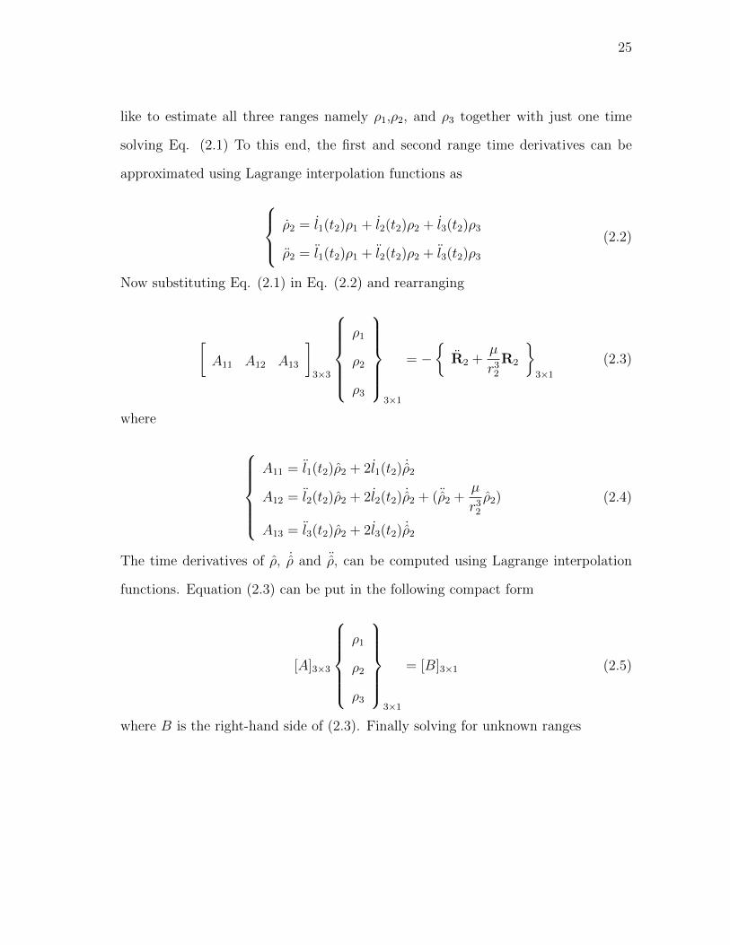
like to estimate all three ranges namely ρ1,ρ2, and ρ3 together with just one time
solving Eq. (2.1) To this end, the first and second range time derivatives can be
approximated using Lagrange interpolation functions as
ρ2 = l1(t2)ρ1 + l2(t2)ρ2 + l3(t2)ρ3
ρ2 = l1(t2)ρ1 + l2(t2)ρ2 + l3(t2)ρ3
(2.2)
Now substituting Eq. (2.1) in Eq. (2.2) and rearranging
[A11 A12 A13
]3×3
ρ1
ρ2
ρ3
3×1
= −
R2 +µ
r32R2
3×1
(2.3)
where
A11 = l1(t2)ρ2 + 2l1(t2) ˙ρ2
A12 = l2(t2)ρ2 + 2l2(t2) ˙ρ2 + (¨ρ2 +µ
r32ρ2)
A13 = l3(t2)ρ2 + 2l3(t2) ˙ρ2
(2.4)
The time derivatives of ρ, ˙ρ and ¨ρ, can be computed using Lagrange interpolation
functions. Equation (2.3) can be put in the following compact form
[A]3×3
ρ1
ρ2
ρ3
3×1
= [B]3×1 (2.5)
where B is the right-hand side of (2.3). Finally solving for unknown ranges

26
ρ1
ρ2
ρ3
3×1
= [A]−13×3[B]3×1 (2.6)
Equation (2.6) yields all three ranges together. Also note that the term r32 appears in
both matrices A and B, so no closed-form form solution is available and the unknown
ranges need to be obtained through an iterative procedure. As mentioned earlier,
in the Laplace original algorithm, an eight order polynomial in terms of r2 needs to
be solved and fed back to the set of equations which is a computational burden. To
bypass this drawback, we simply replaced r2 by the equation defining the geometry
of the problem. In the next section, we will see that this modification yields results
comparable to those of the original Laplace method. Also, the initial guess of zero
can be used for all the unknown ranges. In the case of non- coplanar orbits (line-of-
sights not lying on the satellite orbit plane), matrix A is invertible, but in case of
coplanar (line-of-sights are on the satellite orbit plane), Eq. (2.5) collapses into two
while we have three unknown, as a result, matrix A is not full rank and singularity
occurs. The next modification discusses this issue.
When dealing with coplanar cases, at least one more observation is needed to
avoid singularity. Assume we have four observations, so two sets of equations each
looking like Eq. (2.5) can be constructed. Since each set contains two scaler equa-
tions, so the total of four equations would be sufficient to solve for the four unknown
ranges. After combining the two sets, we have

27
A11 A12 A13 03×1
03×1 A22 A23 A24
6×4
ρ1
ρ2
ρ3
ρ4
4×1
= −
R2 +
µ
r32R2
R3 +µ
r33R3
6×1
(2.7)
where
A11 = l1(t2)ρ2 + 2l1(t2) ˙ρ2
A12 = l2(t2)ρ2 + 2l2(t2) ˙ρ2 + (¨ρ2 +µ
r32ρ2)
A13 = l3(t2)ρ2 + 2l3(t2) ˙ρ2
.....................................
A22 = l1(t3)ρ3 + 2l1(t3) ˙ρ3
A23 = l2(t3)ρ3 + 2l2(t3) ˙ρ3 + (¨ρ3 +µ
r33ρ3)
A24 = l3(t3)ρ3 + 2l3(t3) ˙ρ3
(2.8)
or in a compact form
[A]6×4
ρ1
ρ2
ρ3
ρ4
4×1
= [B]6×1 (2.9)
and finally

28
ρ1
ρ2
ρ3
ρ4
4×1
= ([AT ][W ][A])−14×4[AT ]4×6[W ][B]6×1 (2.10)
where W is a weight matrix. Note that even in the case of coplanar, ATA is full rank
and hence invertible. In case of multiple observations, Eq. (2.9) can be generalized
and written in the following form
A11 A12 A13 03×1 ... 03×1
03×1 A22 A23 A24 ... 03×1
......
...... ...
...
03×1 03×1 ... A(n−2)(n−2) A(n−2)(n−1) A(n−2)(n)
ρ1
ρ2...
ρn
=
−
R2 +µ
r32R2
R3 +µ
r33R3
...
Rn−1 +µ
r3n−1Rn−1
(2.11)
and then solution for the unknown ranges
ρ1
ρ2...
ρn
n×1
= ([AT ][W ][A])−1n×n[AT ]n×3(n−2)[W ][B]3(n−2)×1 (2.12)
where W is a weight matrix. Using more observations than three, not only fixes the
singularity issue, but enhances the accuracy of the estimated satellite position and

29
velocity vector.
D. Selected Test Scenarios and Results
The validation and effectiveness of the developed modifications were tested through
several different scenarios. All the observations were made from a ground-based site
located at a point of zero longitude and zero latitude for the sake of simplicity. To
simulate the real data, the ideal measured data were corrupted with Gaussian noise
with standard deviation of 3σ = 10arcsec. The estimated error are presented in
terms of orbit shape and orbit orientation. In the following subsection, the orbit
shape and orbit orientation error is briefly introduced.
1. Non-coplanar Scenarios
To test the performance of the modified and original algorithms, a Monte Carlo
analysis was conducted using 2326 different scenarios. A random orbit generator
was used for the purpose. The orbits have eccentricity ranging from 0 to 0.2 and
inclination angle from 5 to 90. The coplanar scenarios were not included in this first
part of the analysis as the original Laplace (with three observations) shows singularity
for coplanar cases. For each scenario, the orbital elements were calculated using the
original and modified Laplace algorithms and then the results were compared both
qualitatively and quantitatively. To have a better feeling of the performances of the
different algorithms used, we collected the estimated a and b with relative percentage
error up to 1% (defined as 100×|true−estimated|/true) and Φ up to 1. Out of 2326
scenarios, the original Laplace, and modified Laplace with 3,4,5, and 6 observations
yielded 194, 294, 410, 533, and 585 occurrences respectively. Table II presents the
results of this analysis.

30
Table II. Non-Coplanar Monte Carlo Analysis for 2326 LEO Scenarios (3σ = 10” and
∆t = 10s)
Laplace Original n = 3 n = 4 n = 5 n = 6
Occurrences 194 294 410 533 585
Percentage (%) 8.4 12.6 17.6 22.9 25.2
As can be seen, with more number of observations used, more scenarios fall into the
specified error zone (aerror < %1, berror < %1,Φ < 1). For example, the performance
of the modified Laplace with number of observations n = 6 gets three times better
than that of the original Laplace. Apart from this qualitative analysis, we also were
interested in testing some specific scenarios as quantitative comparison. So, one
random case was considered. The orbital elements of this scenario is presented in
Table III.
Table III. Orbital Elements for a Single Random Scenario: Non-coplanar
Scenario a e i Ω ω ϕ
km [-] (deg) (deg) (deg) (deg)
Non-coplanar 7,800.0 0.1 45 345 15 0
Tables IV presents the semi-major axis and semi-minor axis relative percentage er-
rors, attitude error matrix principal angle, and CPU time. As can be seen, as the
number of observations increases, the accuracy of the estimated orbit shape and ori-
entation improves with no significant change in the CPU time. Note how the results
improve from Laplace original to Laplace with n = 6 for both orbit shape and orien-
tation errors. The original Laplace yields poor results for the near-earth orbits, but
as it can be seen, the modified Laplace can successfully be used for the LEO orbit
determination problems.

31
Table IV. Performance Comparison of Original and Modified Laplace for One Single
Non-coplanar Scenario (3σ = 10” and ∆t = 10s)
Algorithms aerror(%) berror(%) Φ (deg) Elapsed Time (s)
(Laplace)
Original 0.72 0.68 14.8 0.014
n=3 0.56 0.53 35 0.011
n=4 0.2 0.19 0.03 0.011
n=5 0.06 0.059 0.028 0.012
n=6 0.018 0.015 0.027 0.013
2. Coplanar Scenarios
As mentioned in the forgoing, the original Laplace method shows singularity when
dealing with coplanar cases (line-of-sights are lying on the satellite orbit plane).
To bypass this drawback, at least one more observation needs to be added to the
set of equations. To test the performance of the developed modified algorithm,
a Monte-Carlo analysis was conducted for 2212 coplanar cases. A random orbit
generator was used for the purpose. The orbits have the semi-major axis ranging
from 6768.324km to 9621.290km and eccentricity ranging from 0 to 0.2. Again,
we collected the estimated a and b with relative percentage error up to 1% and the
angular momentum vector error θup to 1 as the specified error zone. Note that since
for the coplanar cases, the Right Ascension Ascending Node Ω is indefinable, so the
orbit orientation error criterion used for the non-coplanar cases can not be used for
coplanar scenarios. So instead, the angle between the true and estimated angular
momentum vectors θ was used as the indication of the orbit orientation error. The
noise with 3σ = 10” and time interval of ∆t = 15s were used for the analysis. Out of
2212 scenarios, the modified Laplace with 4,5, and 6 observations yielded 153, 341,

32
and 482 occurrences respectively. This shows that as the number of observations
increase, the estimation accuracy improves. Table V presents a summary of this
Monte Carlo analysis.
Table V. Coplanar Monte Carlo Analysis for 2212 LEO Scenarios (3σ = 10” and
∆t = 10s)
Laplace n = 4 n = 5 n = 6
Occurrences 153 341 482
Percentage (%) 6.9 15.4 21.8
Table VI presents the orbit elements of a single scenario and Table VII presents the
results using the modified Laplace using number of observations 4, 5, and 6. The
angle between the true and estimated angular momentum vectors θ was used as the
orbit orientation error criterion.
Table VI. Orbital Elements for a Single Random Scenario: Coplanar
Scenario a e i Ω ω ϕ
km [-] (deg) (deg) (deg) (deg)
Coplanar 7,602.35 0.034 0 0 2.45 0
Table VII. Performance Comparison of the Modified Laplace for One Single Coplanar
Scenario (3σ = 10” and ∆t = 10s)
Algorithms aerror(%) berror(%) θ (deg) Elapsed Time (s)
(Laplace)
n=4 2.17 1.57 0.0038 0.012
n=5 0.54 0.06 0.0037 0.012
n=6 0.027 0.0095 0.0037 0.013
33
As can be seen, the CPU time and orientation error remain almost the same whereas
the orbit shape error improves significantly.
E. Conclusion
Three modifications were made to the Original Laplace method of initial orbit de-
termination and successfully tested. The first modification eliminates the need for
solving an eighth order polynomial in the original Laplace algorithm. As the second
modification, the unknown ranges can be estimated all together while the original
method offers just one unknown range at a time. In the third modification, the
Laplace method was generalized to multiple observations which makes it suitable for
dealing with the coplanar cases as the original Laplace shows singularity for copla-
nar orbit determination problems. Two Monte Carlo Analysis were performed for
both coplanar and non-coplanar scenarios. The modified Laplace algorithm showed
much better results compared to those of the original Laplace whereas the CPU time
remained almost the same. The error presented in this work are in terms of orbit
error which contains both orbit shape and orbit orientation errors. The time interval
between the measurements was considered ∆t = 15s with the measurement noise of
3σ = 10”. As the time interval increases, the measurements are less affected by the
noise, but in turn, the approximated quantities lose accuracy, and as the time inter-
val decreases, the approximation would be more accurate, but the measurements are
more affected by the noise. So, there is an optimal time interval with respect to the
level of the noise involved in the measurements. The original Laplace yields poor re-
sults for LEO orbit determination problems, whereas the modified algorithm showed
reasonable results for the near-earth orbits. The Lagrange interpolation polynomials
were used for the approximation purposes which may not be the best way to do so.

34
The least square technique and using some other sort of functions can be tried as an
alternative for the Lagrange interpolation functions.

35
CHAPTER III
INITIAL ORBIT DETERMINATION USING MULTIPLE OBSERVATIONS
In this chapter, two new angles-only initial orbit determination techniques are pre-
sented.
A. Introduction
With the advent of the space age, more computer-based algorithms with iterative
nature were developed among which the Double r-iteration technique by Escobal [12]
and, more recently, the new approach by Gooding [13], which are both angles-only
methods, can be mentioned. Basically, in the Double r-iteration method, the mean
anomaly and the mean motion are computed based on the estimated ranges (initial
guess) and then the residuals defined as the difference between the real time interval
(between the measured observations) and estimated time interval (mean anomaly
divided by mean motion) are tried to be minimized with respect to the unknown
range. The solution is achieved when the residuals become smaller than some pre-
scribed tolerance. Laplace’s doesn’t exhibit acceptable performance for near-Earth
satellites and only yields good results on the middle range (the second range out of
three observations). Gauss’ method offers good results on all three computed ranges
and is more accurate for near-Earth satellites than Laplace’s, obtaining its best ac-
curacy when the measured data are less than 10 apart [3]. Gauss’s and Laplace’s
methods exhibit singularity on coplanar orbit determination problems, namely, when
the observed line-of-sight vectors all lie on the observer’s orbital plane. The Dou-
ble r-iteration method is based on the iterative improvement of estimates for the
first and last ranges. This method is, unlike Gauss’, effective for large spreads in
the observations, but suffers from some limitations such as very limited initial guess

36
converging region and is less stable when dealing with real data corrupted by noise
(as compared to the techniques proposed here). Gooding method yields multiple
solutions including the all zero-range trivial solution on space-based orbit estimation
problems (e.i., satellite tracking satellite). Another drawback of the Gooding method
is that the initial guess should be close enough to the true values which results in
failure when too noisy data are used. The presented technique yields an acceptable
robustness with respect to the noise levels and initial guess. The methods using three
angles-only observations typically become more complex if they are to be modified
for multiple observations, whereas the complexity of the proposed techniques does
increase with the number of observations. The algorithm presented in this chapter
relies on the fact that, for unperturbed Keplerian orbits, all position vectors lie on
the same (orbital) plane and uses the Lagrangian coefficients, f and g, similarly to
Gauss’ method. For this reason, the proposed technique is compared to the clas-
sic methods of Gauss’ as they have been constructed on the same foundation and
compared with the Double r-iteration, as they both are iterative techniques.
The four particular features of the presented method are:
1. capable of using multiple observations;
2. does not show singularity for coplanar angles-only orbit determination prob-
lems;
3. does not converge to the trivial solution for space-based applications, and
4. exhibits more robustness to the initial guess with a larger region of convergence.
In the following section, the formulation development for three and multiple ob-
servations is introduced. Then, the subsequent section deals with the performance of
the presented method. Finally, four scenarios will be considered to test the perfor-
37
mance and to validate the proposed method. In particular, the observed lines-of-sight
directions are corrupted with Gaussian noise to simulate real observations.
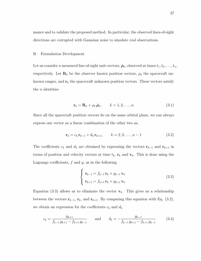
B. Formulation Development
Let us consider nmeasured line-of-sight unit-vectors, ρk, observed at times t1, t2, . . . , tn,
respectively. Let Rk be the observer known position vectors, ρk the spacecraft un-
known ranges, and rk the spacecraft unknown position vectors. These vectors satisfy
the n identities
rk = Rk + ρk ρk, k = 1, 2, . . . , n (3.1)
Since all the spacecraft position vectors lie on the same orbital plane, we can always
express one vector as a linear combination of the other two as,
rk = ck rk−1 + dk rk+1, k = 2, 3, . . . , n− 1 (3.2)
The coefficients ck and dk are obtained by expressing the vectors rk−1 and rk+1 in
terms of position and velocity vectors at time tk, rk and vk. This is done using the
Lagrange coefficients, f and g, as in the following rk−1 = fk−1 rk + gk−1 vk
rk+1 = fk+1 rk + gk+1 vk
(3.3)
Equation (3.3) allows us to eliminate the vector vk. This gives us a relationship
between the vectors rk−1, rk, and rk+1. By comparing this equation with Eq. (3.2),
we obtain an expression for the coefficients ck and dk
ck =gk+1
fk−1 gk+1 − fk+1 gk−1and dk = − gk−1
fk−1 gk+1 − fk+1 gk−1(3.4)
38
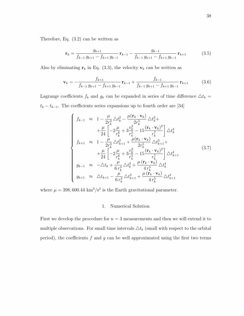
Therefore, Eq. (3.2) can be written as
rk =gk+1
fk−1 gk+1 − fk+1 gk−1rk−1 −
gk−1fk−1 gk+1 − fk+1 gk−1
rk+1 (3.5)
Also by eliminating rk in Eq. (3.3), the velocity vk can be written as
vk = − fk+1
fk−1 gk+1 − fk+1 gk−1rk−1 +
fk−1fk−1 gk+1 − fk+1 gk−1
rk+1 (3.6)
Lagrange coefficients fk and gk can be expanded in series of time difference 4tk =
tk − tk−1. The coefficients series expansions up to fourth order are [34]
fk−1 ≈ 1− µ
2r3k4t2k −
µ(rk · vk)2r5k
4t3k+
+µ
24
[−2
µ
r6k+ 3
v2kr5k− 15
(rk · vk)2
r7k
]4t4k
fk+1 ≈ 1− µ
2r3k4t2k+1 +
µ(rk · vk)2r5k
4t3k+1+
+µ
24
[−2
µ
r6k+ 3
v2kr5k− 15
(rk · vk)2
r7k
]4t4k+1
gk−1 ≈ −4tk +µ
6 r3k4t3k +
µ (rk · vk)4 r5k
4t4k
gk+1 ≈ 4tk+1 −µ
6 r3k4t3k+1 +
µ (rk · vk)4 r5k
4t4k+1
(3.7)
where µ = 398, 600.44 km3/s2 is the Earth gravitational parameter.
1. Numerical Solution
First we develop the procedure for n = 3 measurements and then we will extend it to
multiple observations. For small time intervals 4tk (small with respect to the orbital
period), the coefficients f and g can be well approximated using the first two terms

39
of the series expansions, only. This yields [34] to the approximated expressionsck ≈
4tk+1
4tk +4tk+1
[1 + µ
(4tk +4tk+1)2 −4t2k+1
6 r3k
]
dk ≈4tk
4tk +4tk+1
[1 + µ
(4tk +4tk+1)2 −4t2k
6 r3k
] (3.8)
where k = 2, . . . , n− 1 and for equally spaced measured times (4t = const)
ck = dk =1
2
(1 +
µ
2 r3k4t2
)(3.9)
Using the expressions obtained for ck and dk from Eq. (3.9), we can rewrite Eq. (3.2)
in a scalar form. For three lines-of-sight, ρ1, ρ2, and ρ3, we obtain a set of three
algebraic equations in terms of the unknown ranges. This allows us to introduce the
residuals ψj(ρ1, ρ2, ρ3), j = 1, 2, 3, asψ1 = c2(R1,x + ρ1 ρ1,x) + d2(R3,x + ρ3 ρ3,x)− (R2,x + ρ2 ρ2,x)
ψ2 = c2(R1,y + ρ1 ρ1,y) + d2(R3,y + ρ3 ρ3,y)− (R2,y + ρ2 ρ2,y)
ψ3 = c2(R1,z + ρ1 ρ1,z) + d2(R3,z + ρ3 ρ3,z)− (R2,z + ρ2 ρ2,z)
(3.10)
Hence, the searched solution must satisfy
ψj(ρ∗1, ρ
∗2, ρ
∗3) = 0, j = 1, 2, 3. (3.11)
Let us now write the Taylor’s series expansion of Eq. (3.10) up to the 2nd order
ψi+1 ≈ ψi + Ji4ρi +1
24ρT
iHi4ρi (3.12)
where
40
Ji =
∂ψ1i
∂ρ1
∂ψ1i
∂ρ2
∂ψ1i
∂ρ3
∂ψ2i
∂ρ1
∂ψ2i
∂ρ2
∂ψ2i
∂ρ3
∂ψ3i
∂ρ1
∂ψ3i
∂ρ2
∂ψ3i
∂ρ3
and Hi =
∂2ψi
∂ρ21
∂2ψi
∂ρ1∂ρ2
∂2ψi
∂ρ1∂ρ3
∂2ψi
∂ρ2∂ρ1
∂2ψi
∂ρ22
∂2ψi
∂ρ2∂ρ3
∂2ψi
∂ρ3∂ρ1
∂2ψi
∂ρ3∂ρ2
∂2ψi
∂ρ23
(3.13)
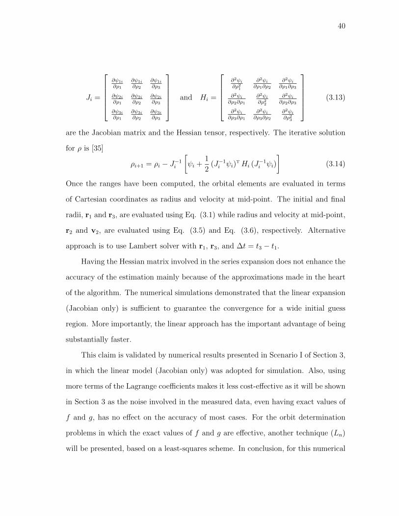
are the Jacobian matrix and the Hessian tensor, respectively. The iterative solution
for ρ is [35]
ρi+1 = ρi − J−1i[ψi +
1
2(J−1i ψi)
THi (J−1i ψi)
](3.14)
Once the ranges have been computed, the orbital elements are evaluated in terms
of Cartesian coordinates as radius and velocity at mid-point. The initial and final
radii, r1 and r3, are evaluated using Eq. (3.1) while radius and velocity at mid-point,
r2 and v2, are evaluated using Eq. (3.5) and Eq. (3.6), respectively. Alternative
approach is to use Lambert solver with r1, r3, and ∆t = t3 − t1.
Having the Hessian matrix involved in the series expansion does not enhance the
accuracy of the estimation mainly because of the approximations made in the heart
of the algorithm. The numerical simulations demonstrated that the linear expansion
(Jacobian only) is sufficient to guarantee the convergence for a wide initial guess
region. More importantly, the linear approach has the important advantage of being
substantially faster.
This claim is validated by numerical results presented in Scenario I of Section 3,
in which the linear model (Jacobian only) was adopted for simulation. Also, using
more terms of the Lagrange coefficients makes it less cost-effective as it will be shown
in Section 3 as the noise involved in the measured data, even having exact values of
f and g, has no effect on the accuracy of most cases. For the orbit determination
problems in which the exact values of f and g are effective, another technique (Ln)
will be presented, based on a least-squares scheme. In conclusion, for this numerical

41
approach, only the first two terms of Taylor’s series expansion and approximated
Lagrange coefficients are adopted. This numerical procedure will be referred to as
Jn throughout this paper, where “J” stands for “Jacobian” and the subscript, n,
indicates the number of observations. The algorithm through which the components
of the Jacobian matrix were constructed is provided in Appendix A.
When the observer position vectors (R1, R2, R3) and the measured lines-of-sight
directions (ρ1, ρ2, ρ3) all lie on the satellite orbit plane, the co-planarity condition
given in Eq. (3.2) collapses into two equations (the third equation becomes zero
as the coordinate perpendicular to the orbit plane vanishes). In this case we have
three unknowns (ρ1, ρ2, and ρ3) and two equations. This is the case referred to
as singularity case. To obtain the solution, a fourth observation is required with
which two co-planarity conditions can be constructed. Now since each co-planarity
condition collapses into two equations for the coplanar case, we obtain a total of four
equations which is sufficient to solve for the four unknown ranges, ρ1, ρ2, ρ3, and ρ4.
2. Extension to Multiple Observations
In the case of n observations (n > 3) more than one coplanarity condition can be
written. For n observations we have
r2 = c2 r1 + d2 r3
r3 = c3 r2 + d3 r4...
rn−1 = cn−1 rn−2 + dn−1 rn
(3.15)

42
By substituting Eq. (3.1) in Eq. (3.15), a set of 3(n− 2) algebraic equations
ψ1 = c2(R1,x + ρ1 ρ1,x) + d2(R3,x + ρ3 ρ3,x)− (R2,x + ρ2 ρ2,x)
...
ψ3(n−2) = cn−1(Rn−2,z + ρn−2 ρn−2,z) + dn−1(Rn,z + ρn ρn,z)+
−(Rn−1,z + ρn−1 ρn−1,z)
(3.16)
is obtained. This set of equation can be written in the compact form
ψj(ρ∗k) = 0, j = 1, 2, . . . , 3(n− 2), k = 1, 2, . . . , n. (3.17)
In general, the Jacobian is a 3(n− 2)× n matrix and not necessarily square, so Eq.
(3.14) becomes (no Hessian involved)
ρi+1 = ρi − (J T
i WJi)−1 J T
i Wψi (3.18)
where W is a weight matrix. The Jacobian J is built as shown in Appendix A.
This technique, called “Jn”, requires building the Jacobian. In the contrary, the
technique presented in the next section does not require constructing the Jacobian
or computing any sort of higher derivatives.
3. Least-Squares Solution
The coplanarity conditions can written in the matrix form, M ρ = ξ, where ρ and ξ
are n× 1 and 3(n− 2)× 1 vectors respectively and M is a 3(n− 2)× n matrix. For
any set of ranges, ρk, we can write (n− 2) vectorial identities
ck ρk−1 ρk−1 − ρk ρk + dk ρk+1 ρk+1 = Rk − (ckRk−1 + dkRk+1) (3.19)

43
where k = 2, 3, . . . , n− 1. Setting ξk = Rk − ckRk−1 − dkRk+1, we can rewrite the
(n− 2) equations given in Eq. (3.19) in the compact matrix form, M ρ = ξ, where
c2ρ1 −ρ2 d2ρ3 0 0 · · · 0
0 c3ρ2 −ρ3 d3ρ4 0 · · · 0
0 0 c4ρ3 −ρ4 d4ρ5 · · · 0
......
......
.... . .
...
0 0 0 0 0 · · · dn−1ρn
ρ1
ρ2
ρ3...
ρn
=
ξ2
ξ3
ξ4...
ξn−1
(3.20)
where 0 identifies a 3 × 1 vector of zeroes. The least-squares solution of Eq. (3.20)
is
ρ = (MTWM)−1 MTWξ (3.21)
Once the range vector, ρ, has been computed, the orbital elements are then evaluated
using Lambert solver with the most orthogonal estimated radii using Eq. (3.1). For
short-arc observations, these are usually the first and the last ones.
Although this procedure is iterative, the initial guess of all ranges set to zero
works efficiently for almost all cases. This technique does not require using approxi-
mated (truncated) values of the Lagrange coefficients, so the exact values of f and g
can be used. This least-squares algorithm will be referred to as Ln throughout this
paper where “L” stands for Least-squares and the index n is the number of observa-
tions. In the examples we have used the Taylor’s series expansion of the Lagrange
coefficients up to the fourth order.
4. Gauss-exact
The accuracy of the original Gauss method (approximate Lagrange coefficients) can
be enhanced by using the exact values of the coefficients. Reference [36] explains how
this can be achieved using the exact values of the coefficients f and g and Universal

44
Kepler’s Equation. A brief review of the procedure will be explained here for the
sake of completeness. The exact values of the Lagrange coefficients can be written
in terms of the universal anomaly, χ, asf = 1− χ2
r0C(αχ2)
g = ∆t− 1√µχ3 S(αχ2)
(3.22)
where C and S are Stumpff functions and defined asS(αχ2) =
√αχ2 − sin
√αχ2
(√αχ2)3
C(αχ2) =1− cos
√αχ2
αχ2
(3.23)
and r0 is the magnitude of the initial position vector. The quantity α is defined as
α = 2r0− v20
µwhere v0 is the magnitude of the initial velocity vector.The Universal
Kepler’s Equation in terms of universal anomaly
√µ∆t =
r0vr0√µχ2C(αχ2) + (1− αr0)χ3S(αχ2) + r0χ (3.24)
here vr0 is the magnitude of the tangential component of the velocity vector. The
solution of Eq. (3.24), χ, then will be plugged back into Eq. (3.22) to obtain the
exact values of f and g.
C. Simulations and Results
Four different scenarios were used for testing and validation. In all cases, the mea-
surements were made from a ground tracking site located at a zero longitude and
zero latitude for the sake of simplicity. The results from the developed techniques
were compared with those of Gauss, Double r-iteration, and improved Gauss which
is referred to as Gauss-exact here. The accuracy of the original Gauss method (using

45
approximated Lagrange coefficients) can be enhanced by using the exact values of
the coefficients. Reference [3] (Algorithm 5.6) explains how this can be achieved
using the exact values of the coefficients f and g and universal Kepler’s equation. To
simulate the true measurements, the ideal data were corrupted with Gaussian noise
with standard deviation of σ = 5′′. The ideal measured lines-of-sight were simulated
through the following procedure:
(a) Orbital elements of a typical low earth orbit (LEO) were selected. The orbital
elements selection was made consistent with the observation site selection so that
the observed satellite is actually in view.
(b) The initial position and velocity vectors are then obtained using the orbital
elements selected from the previous step.
(c) The satellite initial position and velocity vectors (initial condition) are then prop-
agated using the Keplerian two-body problem to obtain subsequent observations,
rk, k = 1, 2, . . . , n, which are the ideal position vectors.
(d) Since we know where the ground observer is located, the Rk vectors are already
known.
(e) The ideal measured lines-of-sight ρk, are then obtained using Eq. (3.1).
The initial satellite real position and velocity vectors of each scenario can be
found in Table VI. The observer position vector is the same for all scenarios. The
initial position vector of the ground tracking site is R1 = 6, 378.137, 0, 0T km.
Using these data, the real (ideal) lines-of-sight vectors can be calculated following
item (e), mentioned above. The estimated error presented in all four scenarios is
in terms of relative position percentage error defined as error (%) = 100 (|rest −

46
rtrue|)/|rtrue|. Finally, the errors provided in the Tables and Figures are obtained by
averaging the estimated error of each observation.
1. Scenario I: Tracking equatorial LEO satellite (coplanar case). The first test is
dedicated to compare the performance of the presented technique for a coplanar
case. Comparisons were made with respect to Gauss’ method as it is (along
with Laplace’s) not capable of handling the coplanar case problem. In this
scenario, where the measured directions are lying on the satellite orbital plane,
the coplanarity condition, Eq. (3.2), collapses into two algebraic equations.
Since, each coplanarity condition involves three unknown ranges (ρ1, ρ2, ρ3)
in order to obtain the sufficient number of equations, one more observation is
needed. This leads to two coplanarity conditions and a set of four algebraic
equations with four unknown ranges. For this specific case, the satellite orbital
plane is assumed to be lying on the Earth equatorial plane.
The time intervals between the observations was chosen 4t = 50 s. Table
VIII presents the results of our technique versus those of Gauss’ and Double
r-iteration. Table VIII provides the results obtained using Jn and Ln methods
for n > 3 observations.
As it can be seen from Table VIII the number of observation of five is optimal
as, for this specific problem, no accuracy improvement has been experienced
with more observations.
Scenario I was run twice with linear and quadratic theories using 4 observa-
tions. With Hessian term involved, we obtained error (%) = 0.0197 and error
(%) = 0.02 without it. The small increase of accuracy does not fully justify
the substantial complexity increase due to Hessian evaluation.
2. Scenario II: Tracking a 45 LEO satellite (inclined case). In this case, the

47
Table VIII. Tracking Equatorial LEO Satellite (Coplanar Case)
Approach Observations Position Iterations Elapsed
error (%) time (s)
Gauss 3 singular non-iterative N/A
Gauss-exact 3 singular 5 N/A
Double-r 3 diverged 1 N/A
J4 4 0.02 2 0.0082
J5 5 0.016 2 0.0083
J6 6 0.016 2 0.0084
L4 4 0.017 7 0.028
L5 5 0.011 7 0.03
L6 6 0.011 7 0.032
orbit has a 45 inclination, and three observations would be sufficient to obtain
the solution. The time interval between the observations was 4t = 50 s. Table
IX shows the results for n = 3 as well as for multiple observations using Jn and
Ln methods.

48
Table IX. Tracking a 45 deg. LEO Satellite (Inclined Case)
Approach Observations Position Iterations Elapsed
error (%) time (s)
Gauss 3 0.06 non-iterative 0.036
Gauss-exact 3 0.06 5 0.05
Double-r 3 0.06 3 0.035
J3 3 0.06 2 0.007
J4 4 0.035 2 0.0084
J5 5 0.030 2 0.0084
J6 6 0.030 2 0.0086
L3 3 0.06 7 0.026
L4 4 0.030 10 0.03
L5 5 0.023 10 0.032
L6 6 0.020 10 0.034

49
3. Scenario III: Tracking a polar LEO satellite (orthogonal case). In this case, a
polar orbit was considered using the same time interval between measurements.
Results are provided in Table X.
Table X. Tracking a Polar LEO Satellite (Orthogonal Case)
Approach Observations Position Iterations Elapsed
error (%) time (s)
Gauss 3 0.18 non-iterative 0.035
Gauss-exact 3 0.18 5 0.05
Double-r 3 0.18 3 0.036
J3 3 0.18 2 0.007
J4 4 0.086 2 0.0083
J5 5 0.07 2 0.0083
J6 6 0.058 2 0.0087
L3 3 0.18 10 0.027
L4 4 0.083 12 0.031
L5 5 0.06 15 0.035
L6 6 0.052 16 0.04
4. Scenario IV: Tracking an asteroid (hyperbolic case). In this case, an astroid
flying by the Earth on a hyperbolic orbit was considered with 4t = 50 s to
be consistent with the other three previous scenarios. Results are presented
in Table XI. The methods of Jn and Ln were run using multiple observations
again for results accuracy enhancement.
The technique Jn yields the same accuracy level over a wide range of initial
guess, from almost 0.5 to 10 times of the true solution. The technique Ln

50
Table XI. Tracking an Asteroid on Hyperbolic Orbit
Approach Observations Position Iterations Elapsed
error (%) time (s)
Gauss 3 0.021 non-iterative 0.026
Gauss-exact 3 0.021 5 0.1
Double-r 3 0.021 5 0.052
J3 3 0.021 2 0.007
J4 4 0.019 2 0.008
J5 5 0.017 2 0.0082
J6 6 0.018 2 0.0084
L3 3 0.021 7 0.026
L4 4 0.018 7 0.03
L5 5 0.014 7 0.032
L6 6 0.014 7 0.034
can work with almost every initial guess whereas the Double r-iteration is so
sensitive to the initial guess with very smaller initial guess convergence region
as compared to the proposed techniques.
Tables XII and XIII present the orbital elements of the four scenarios and initial real
position and velocity vectors respectively.
1. Sensitivity Analysis
This section demonstrates that the orbit estimation accuracy mainly depends on
noise level, time intervals between measurements, and the specific selection of orbital
elements. Also different observations combinations were tried to see how the accuracy
of the results would be affected. To quantify the contribution of these parameters to
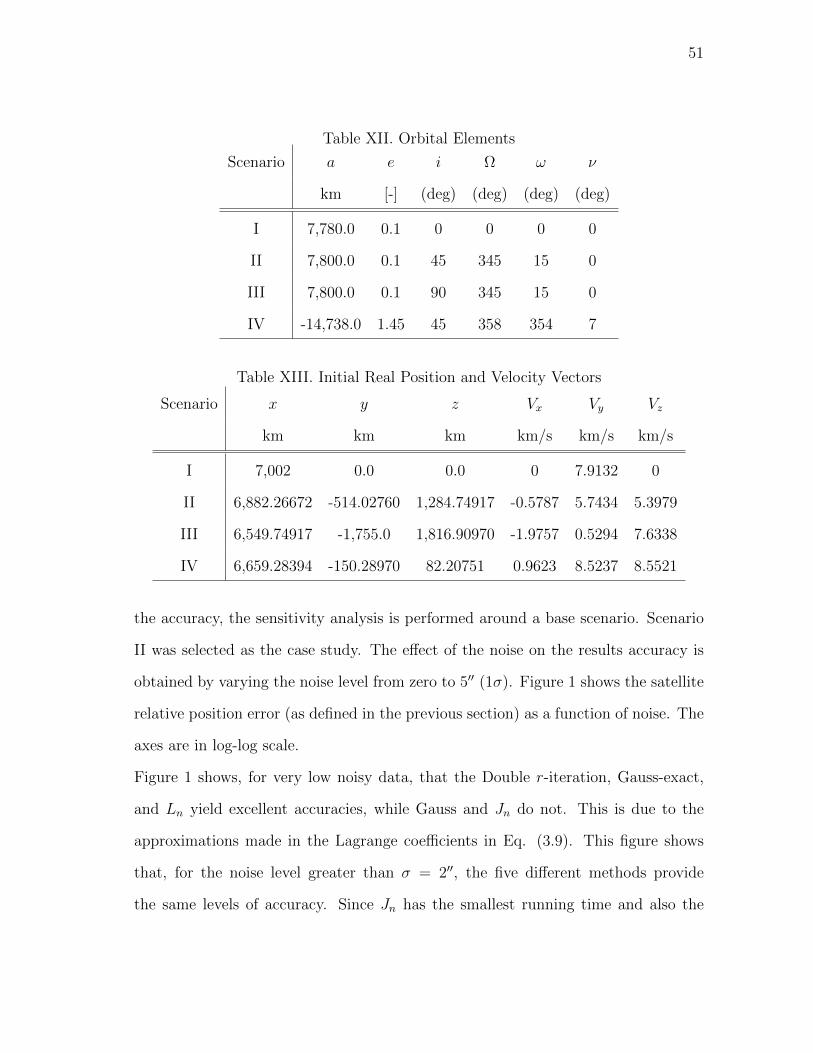
51
Table XII. Orbital Elements
Scenario a e i Ω ω ν
km [-] (deg) (deg) (deg) (deg)
I 7,780.0 0.1 0 0 0 0
II 7,800.0 0.1 45 345 15 0
III 7,800.0 0.1 90 345 15 0
IV -14,738.0 1.45 45 358 354 7
Table XIII. Initial Real Position and Velocity Vectors
Scenario x y z Vx Vy Vz
km km km km/s km/s km/s
I 7,002 0.0 0.0 0 7.9132 0
II 6,882.26672 -514.02760 1,284.74917 -0.5787 5.7434 5.3979
III 6,549.74917 -1,755.0 1,816.90970 -1.9757 0.5294 7.6338
IV 6,659.28394 -150.28970 82.20751 0.9623 8.5237 8.5521
the accuracy, the sensitivity analysis is performed around a base scenario. Scenario
II was selected as the case study. The effect of the noise on the results accuracy is
obtained by varying the noise level from zero to 5′′ (1σ). Figure 1 shows the satellite
relative position error (as defined in the previous section) as a function of noise. The
axes are in log-log scale.
Figure 1 shows, for very low noisy data, that the Double r-iteration, Gauss-exact,
and Ln yield excellent accuracies, while Gauss and Jn do not. This is due to the
approximations made in the Lagrange coefficients in Eq. (3.9). This figure shows
that, for the noise level greater than σ = 2′′, the five different methods provide
the same levels of accuracy. Since Jn has the smallest running time and also the

52
Fig. 1. Scenario II:Relative Position Percentage Error vs. Noise (4t = 50 s)
running time almost remains the same regardless of the number of observations Jn
can be considered the most cost-effective approach. In fact, the computation of the
exact values of the Lagrange coefficients becomes worthless when higher levels of
noise are considered. To avoid this drawback, an increase in the time interval can be
considered. This reduces the noise effect on the accuracy. However, increasing 4t
has technical limitations. For instance, since the tracking site field-of-view is limited,
all measurements should be made within some specific time range.
To see the effect of the time interval ∆t on the accuracy of the results, Scenario
II was solved again for the time intervals varying from 20 s to 120 s. In this case, the
noise level was considered σ = 5′′. Figure 2 shows that increasing the time interval
has caused an accuracy improvement in all five schemes up to ∆t = 60 s. But for
the time intervals larger than almost 60 s, the performance of Jn and Gauss drop as
the Lagrange coefficients used in these two methods are approximated. Since Gauss-

53
Fig. 2. Scenario II:Relative Position Percentage Error vs. Time Interval 4t (σ = 5′′)
exact and Ln use almost the exact values of f and g, the accuracy gets better as
the time interval increases. The number of observations used for this case was three.
Also to see how the estimated position error would be improved with more number
of observations, Ln was run with n = 4, 5, and 6. Figure 3 shows the performance
of Ln versus those of Gauss-exact and Double r-iteration. The technique Ln seems
to be the most suitable one as it can take care of multiple observations for higher
accuracy with almost the same running time as Double r-iteration and Gauss-exact.
Another factor affecting the results accuracy is the orbital elements. The technique
adopted for these tests was Jn. Figure 4 shows how the estimated position error
changes versus the eccentricity, semi-major axis, and true anomaly, respectively. In
this part of the sensitivity analysis, the time interval, ∆t = 50 s, remains constant.
In the first plot of Fig. 4, the eccentricity was changed from zero to 0.25 while the

54
Fig. 3. Scenario II:Performance of Ln vs Double r-iteration and Gauss-exact vs. Time
Interval 4t (σ = 5′′)
other five orbital elements were kept constant. As it can be seen, the accuracy of the
estimated orbit varies versus the orbit eccentricity. The semi-major axis was then
changed from 7,500 km to 10,000 km. The results accuracy is given in the middle
plot of Fig. 4. At last, the true anomaly was changed from 355 to 5 and the results
can be seen in the bottom plot of Fig. 4. In all three plots, the right ascension
(Ω = 345), argument of perigee (ω = 15), and inclination (i = 45) remained
constant. Note that the error behavior shown in Fig. 4 may differ case by case.
Also two more combinations (rather than the original one) of the observations were
tested to see how the accuracy of the results would change. For the purpose, 5
observations were considered out of which three coplanarity conditions could be
written. The original combination is 123, 234, and 345 referred to as Set I here.

55
Fig. 4. Scenario II: Relative Position Percentage Error Sensitivity to Orbital Ele-
ments. Top: Eccentricity, Middle: Semi-major Axis, Bottom: True Anomaly.
(Ω = 345, ω = 15, i = 45), (∆t = 50 s, using Jn)
Two more combinations are: Set II (125,235,245) and Set III (124,135,245). Figure
5 shows all three sets of data exhibit almost same performance over a wide range of
time intervals.
2. Results Bias
Scenario II was selected for the bias test with three observations and 4t = 50 s.
While evaluating the performance of the orbit determination methods used in this
paper, the results of Gauss and Jn were found biased whereas Gauss-exact, Double r-
iteration, and Ln were not. Gauss and Jn are biased because they use approximated
Lagrange coefficients. Figure 6 and 7 show the histograms of the error provided
by Jn and Ln, respectively. To construct these histograms, the orbit determination
problem was run 2,000 times using Ln and Jn. To simulate the true measurements,
the ideal data were corrupted with noise (σ = 5′′) and the respective relative position
error was recorded. Then, the error was plotted versus the number of occurrences for

56
Fig. 5. Scenario II: Relative Position Percentage Error of Different Observations Com-
binations vs. Interval 4t (σ = 5′′)
each amount of error. As it can be seen in Fig. 6, the mean value of the estimated
errors using Jn is about 0.01% (off-set from zero) whereas that of Ln is zero which
is because of using the exact (or very close to exact) values of f and g functions in
Ln. The estimated error presented in the histograms is in terms of relative position
percentage error defined as error (%) = 100 (|rest| − |rtrue|)/|rtrue|. Note that this
definition is slightly different from the one defined in the beginning of this section.
The reason is also to show negative errors when plotting the histograms.
For all the above simulations, the time interval between the measurements was
considered constant and the number of observations was chosen manually by the
operator. The algorithm developed in [37] explains how an optimal combination of
Nobs and ∆t can be achieved.
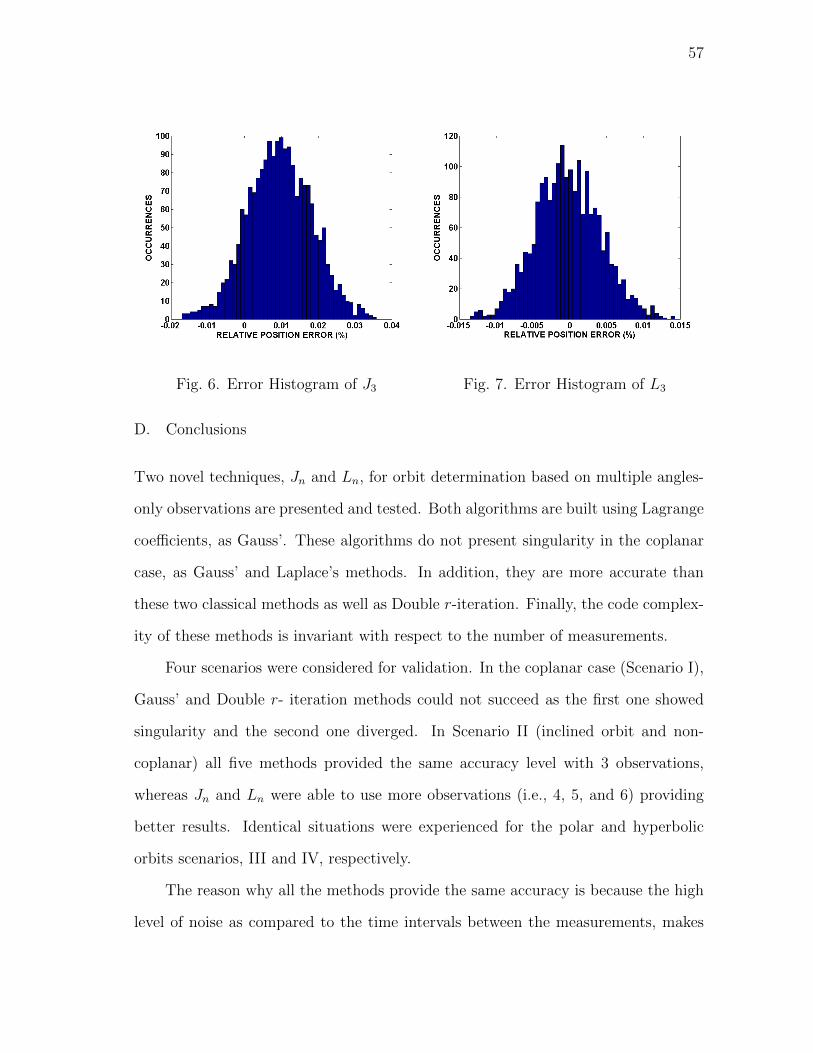
57
Fig. 6. Error Histogram of J3 Fig. 7. Error Histogram of L3
D. Conclusions
Two novel techniques, Jn and Ln, for orbit determination based on multiple angles-
only observations are presented and tested. Both algorithms are built using Lagrange
coefficients, as Gauss’. These algorithms do not present singularity in the coplanar
case, as Gauss’ and Laplace’s methods. In addition, they are more accurate than
these two classical methods as well as Double r-iteration. Finally, the code complex-
ity of these methods is invariant with respect to the number of measurements.
Four scenarios were considered for validation. In the coplanar case (Scenario I),
Gauss’ and Double r- iteration methods could not succeed as the first one showed
singularity and the second one diverged. In Scenario II (inclined orbit and non-
coplanar) all five methods provided the same accuracy level with 3 observations,
whereas Jn and Ln were able to use more observations (i.e., 4, 5, and 6) providing
better results. Identical situations were experienced for the polar and hyperbolic
orbits scenarios, III and IV, respectively.
The reason why all the methods provide the same accuracy is because the high
level of noise as compared to the time intervals between the measurements, makes

58
the calculation of the exact values of the Lagrange functions worthless. For this
reason Jn can be seen as the most cost-effective method as it has the least running
time, almost independent from the number of observations. By increasing the time
intervals, having the exact values of the Lagrange coefficients makes the method
more accurate. For this reason the Ln technique becomes the most suitable.
In general, when the noise level is lower than σ = 2′′, Double r-iteration, Gauss-
exact, and Ln give great accurate results, but as the noise level increases, the es-
timated position errors become as accurate as those of Jn and Gauss. Increasing
the number of observations improves the accuracy. However, the accuracy increase
becomes smaller and smaller until it tends to a limit. The orbital elements as well
play a role in the accuracy of the estimated satellite position vectors. For the specific
scenario used in the sensitivity analysis section, the error decreased as the eccentric-
ity increased up to a certain point; then the error started growing. In particular,
the error decreased as the semi-major axis and true anomaly increased. These be-
haviors are case-depended. Also three different combinations of observations were
tried and all three yielded almost the same accuracy for a wide range of time in-
tervals. Finally, this study has shown that the results from Jn is biased as it uses
approximate Lagrange coefficients. In the contrary, Ln exhibits no biased results.
In conclusion, for each specific orbit determination problem there is an optimum
number of observations and time interval for any noise level.
59
CHAPTER IV
INITIAL ORBIT DETERMINATION USING PRESCRIBED ORBITS
In this chapter, a new angles-only initial orbit determination technique based on
prescribed orbits is presented.
A. Introduction
The initial orbit determination method using multiple observations developed so far
have been able to handle many of the ground and space based orbit determination
problems for both near earth and long distance objects including coplanar cases.
These two techniques are so robust with respect to the initial guess selection and
rarely go unstable because of that. The only drawback associated with these two
algorithms is that as the number of observations and/or time intervals between the
measured directions increase, the accuracy does not get any better and in some
cases, it even drops. The IOD method by Paul Herget [10], [11] is also capable of
using multiple observations basically suitable for the comets, meteors, and planets
and suitable for short arcs. The presented technique was developed in an effort to
be able to handle all the orbit determination scenarios as much as possible with a
higher accuracy compared to the available orbit determination methods, bypassing
the drawbacks and keeping the advantages . The presented technique is also able
to deal with one of the most challenging IOD problems, a co-planar case as the
classic methods of Gauss and Laplace, and Double-r iteration show singularity and
instability when used for coplanar cases. In this technique, an assumed solution
is forced to satisfy both the geometry of the problem and also the Keplerian two-
body problem equation. For the sake of this work, a polynomial was used. In the
next section, the algorithm will be explained in details. Two ways to present the
60
results and performance of the current method compared to those of previous ones
are considered. The error in terms of shape and orientation of the estimated orbit
and error in terms of estimated position vector. Monte Carlo analysis was performed
along with three specific LEO satellite scenarios. The results show the developed
technique is dominant over the classis and recently developed IOD methods by the
authors from every aspect.
B. Algorithm Development
The main idea of this technique is to assume a solution to the Keplerian two-body
problem (no need to solve it and obtain the exact solution) and also enforce the
approximated solution to satisfy the geometry of the problem. The approximated
solution could be a polynomial or any other function best describing that part of orbit
under determination. The algorithm is first developed with a 3-rd order polynomial
to describe the methodology, but the results will be generated using a 5-th order
polynomial. A 5-th order polynomial was accurate enough to handle almost all the
scenarios. The geometry of a typical orbit determination problem with n observations
can be written as
ri = Ri + ρi ρi, i = 1, 2, · · · , n (4.1)
where ri and Ri are the i-th spacecraft and tracking site position vectors respectively.
The unknown range ρi is the one to be determined and ρi is the measured direction
(a unit vector) of the spacecraft. The trajectory of an orbiting object should satisfy

61
the two-body problem. Let us now assume an approximated solution in the form ofx(t) = px(t)
y(t) = py(t)
z(t) = pz(t)
(4.2)
and by considering a 3-rd order polynomial, we havepx(t) = a1 + a2t+ a3t
2 + a4t3
py(t) = b1 + b2t+ b3t2 + b4t
3
pz(t) = c1 + c2t+ c3t2 + c4t
3
(4.3)
The approximated solution p(t) should also be able to satisfy the geometry Eq.(4.1)
so we have px(ti) ∼= Rx
i + ρxi ρxi
py(ti) ∼= Ryi + ρyi ρ
yi , i = 1, 2, · · · , n
pz(ti) ∼= Rzi + ρzi ρ
zi
(4.4)
where ti is the ith measured time. By taking the left hand side of Eq.(4.4) to the
right, we can define the residuals asφxi = −px(ti) + (Rx
i + ρxi ρxi )
φyi = −py(ti) + (Ryi + ρyi ρ
yi ), i = 1, 2, · · · , n
φzi = −pz(ti) + (Rzi + ρzi ρ
zi )
(4.5)
and
Φx =1
2
n∑i=1
φ2xi
Φy =1
2
n∑i=1
φ2yi, i = 1, 2, · · · , n
Φz =1
2
n∑i=1
φ2zi
(4.6)
To have the best fit, the residuals φx, φy, and φz should be minimum with respect

62
to the polynomial coefficients ak, bk, and ck, k = 1, 2, 3, 4. So by applying the least
square scheme, the coefficients can be determined in terms of the unknown ranges asa = T−1[
∑ni=1(R
xi + ρxi ρ
xi )
∑ni=1(R
xi + ρxi ρ
xi )ti ...
∑ni=1(R
xi + ρxi ρ
xi )t
3i ]
T
b = T−1[∑n
i=1(Ryi + ρyi ρ
yi )
∑ni=1(R
yi + ρyi ρ
yi )ti ...
∑ni=1(R
yi + ρyi ρ
yi )t
3i ]
T
c = T−1[∑n
i=1(Rzi + ρzi ρ
zi )
∑ni=1(R
zi + ρzi ρ
zi )ti ...
∑ni=1(R
zi + ρzi ρ
zi )t
3i ]
T
(4.7)
where a = a1 a2 a3 a4T, b = b1 b2 b3 b4T, c = c1 c2 c3 c4T,
and T is 3× 3 matrix
T =
n∑n
i=1 ti ...∑n
i=1 t3i∑n
i=1 ti∑n
i=1 t2i ...
∑ni=1 t
4i
... ... ... ...∑ni=1 t
3i
∑ni=1 t
4i ...
∑ni=1 t
6i
(4.8)
Up to now, the polynomial coefficients have been eliminated and we have them in
terms of the unknown ρi . The next step towards completing the algorithm is enforce
the assumed solution to satisfy the Keplerian two-body problem as the following
px(ti) ∼= −µpx(ti)
[px(ti)2 + py(ti)2 + pz(ti)2]3/2
py(ti) ∼= −µpy(ti)
[px(ti)2 + py(ti)2 + pz(ti)2]3/2, i = 1, 2, · · · , n
pz(ti) ∼= −µpz(ti)
[px(ti)2 + py(ti)2 + pz(ti)2]3/2
(4.9)
or in the residual form
ψxi = px(ti) +µpx(ti)
[px(ti)2 + py(ti)2 + pz(ti)2]3/2
ψyi = py(ti) +µpy(ti)
[px(ti)2 + py(ti)2 + pz(ti)2]3/2, i = 1, 2, · · · , n
ψzi = pz(ti) +µpz(ti)
[px(ti)2 + py(ti)2 + pz(ti)2]3/2
(4.10)
We now define the residual vector as Ψ = [ψxi|ψyi|ψzi]T , i = 1, 2, ..., n. Let us now
63
write Ψ in terms of the Taylor’s series expansion up to the 2-nd order, so we have
ψk+1∼= ψk +4ρT
k [∂Ψ
∂ρ]k +
1
24ρT
k [∂2Ψ
∂ρ2]k4ρk (4.11)
which yields to the iterative solution
ρk+1 = ρk − J−1k[ψk +
1
2(J−1k ψk)
THk (J−1k ψk)
](4.12)
or up to the 1-st order
ρk+1 = ρk − (J T
k WJk)−1 J T
k Wψk, k = 1, 2, ..., n (4.13)
where W is a weight matrix.
C. Example Problems and Results
The performance of the proposed technique was tried to compare with those of Jn and
Ln and the classical method of Gauss. As mentioned in the forgoing, the estimated
error will be expressed in terms of both orbit shape and attitude. Two cases were
considered for validation, coplanar and non-coplanar. The observer was considered
at a point with longitude and latitude of zero for the sake of simplicity and all cases
are ground-based. A random orbit generator was employed to produced different for
obits for the analysis. To simulate the real world data, the ideal measured lines-of-
sights were corrupted with Gaussian noise at the level of 3σ = 10′′. The number
of observations used was Nobs = 7 with two different time intervals, ∆t = 50 s and
∆t = 80 s. We refer to our new technique as Pn (Prescribed Orbits). The index n
denotes the number of observations, so, for instance, P7 means the Prescribed Orbits
method using seven observations. A 5-th order polynomial was used in the proposed
algorithm for the sake of this study.

64
1. LEO Satellite: coplanar orbits In this case, the Monte Carlo analysis was
performed using 2182 different coplanar scenarios with the eccentricity ranging
from 0 to 0.2. The minimum and maximum semi-major axis are 6743.334
km and 9602.719 km respectively. The number of observations of seven with
two different time intervals ∆t = 50s and ∆t = 80s were considered for this
case. Since Gauss’ method shows singularity for coplanar cases, so the three
methods of P7, Jn, and Ln were used for this analysis. The results are presented
in terms of orbit shape error d and the angle between the angular momentum
vectors θ. Figures 8 through 10 show the histograms of the orbit shape error
d and angular momentum vector error θ using Pn, Jn, and Ln for ∆t = 50
s respectively. Figures 11 through 13 are the same plots as the first three,
but for ∆ = 80s. As can be seen, all three methods yielded very good orbit
shape and orientation estimations. The current technique showed much better
estimation of the orbit shape as the time interval ∆t increased , whereas Jn
and Ln exhibited more accurate orientation estimation (in the order of 0.001
deg) as the time interval increases. The orientation error offered by Pn is in
the order of 0.01 deg.

65
Fig. 8. Orbit Shape and Orientation (Angular momentum) Error Using P7, Scenar-
ios=2182
Fig. 9. Orbit Shape and Orientation (Angular Momentum) Error Using J7, Scenar-
ios=2182

66
Fig. 10. Orbit Shape and Orientation (Angular Momentum) Error Using L7, Scenar-
ios=2182
Fig. 11. Orbit Shape and Orientation (Angular Momentum) Error Using P7, Scenar-
ios=2182

67
Fig. 12. Orbit Shape and Orientation (Angular Momentum) Error Using J7, Scenar-
ios=2182
Fig. 13. Orbit Shape and Orientation (Angular Momentum) Error Using
L7,Scenarios=2182

68
2. LEO Satellite: non-coplanar orbits In this case, the Monte Carlo analysis was
performed using 2336 different non-coplanar scenarios with the eccentricity
ranging from 0 to 0.2 and inclination from 5 to 90. The minimum and max-
imum semi-major axis are 6732.241 km and 9634.102 km respectively. The
number of observations of seven with two different time intervals ∆t = 50s
and ∆t = 80s were considered for this case. The methods Pn,Ln do not re-
quire any specific initial guess and basically can operate with any values(Pn
shows extreme robustness with respect to initial guess and Ln algorithm can
be initiated with the value of zero for a fair number of scenarios) and Gauss
does not have an iterative nature. Hereby; these three not required initial guess
IOD methods were used for the non-coplanar scenarios. Results are presented
in terms of orbit shape and attitude phi error. Figures 14 through 16 depict
the histograms of the orbit shape error d and attitude error φ using Pn, Ln,
and Gauss for ∆t = 50s respectively. Figures 17 through 19 are the same
plots as the first three, but for ∆ = 80s. As can be seen, Pn has the highest
accuracy in the orbit shape and attitude estimation. Pn shows more concentra-
tion of attitude error towards the point of zero degree for larger time interval
(∆t = 80s), while Ln and Gauss become more distributed from zero to 0.5.
The histogram of the attitude error φ was plotted up to 0.5. For ∆t = 50s,
the scenarios of 2147, 2214, and 1974 (out of 2336) were used by Pn, Ln, and
Gauss respectively and for ∆t = 80s, the scenarios are 2201, 1939, and 1813
(out of 2336). The best and worst orbit shape estimation belong to P7 and
Gauss (∆t = 80s) respectively.

69
Fig. 14. Orbit Shape and Attitude Error Using P7, Scenarios=2147 out of 2336
Fig. 15. Orbit Shape and Attitude Error Using L7, Scenarios=2214 out of 2336
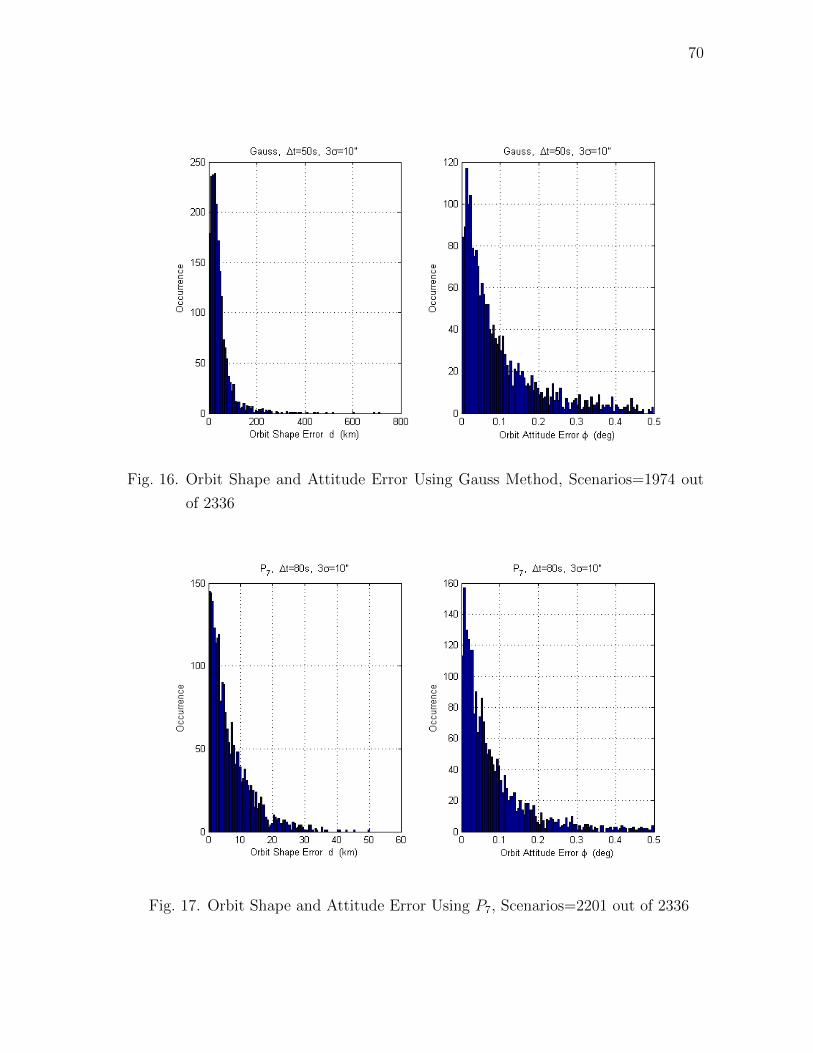
70
Fig. 16. Orbit Shape and Attitude Error Using Gauss Method, Scenarios=1974 out
of 2336
Fig. 17. Orbit Shape and Attitude Error Using P7, Scenarios=2201 out of 2336

71
Fig. 18. Orbit Shape and Attitude Error Using L7, Scenarios=1939 out of 2336
Fig. 19. Orbit Shape and Attitude Error Using Gauss Method, Scenarios=1813 out
of 2336

72
D. Conclusion
A novel technique of IOD based on a prescribed orbit was successfully developed
and tested. The method uses an assumed approximated solution as the solution
to the Keplerian two-body problem. This solution also needs to satisfy the geom-
etry of the problem. So combining these two facts construct the foundation of the
propose technique. Any function which can represent the behavior of an orbit can
be used, but as the first phase of the work and for the sake of simplicity, a 5-th
order polynomial was used and showed promising performance. The performance
of the developed technique was tested versus those of Jn and Ln and classical IOD
method of Gauss. The estimated errors were presented in two ways: 1) orbit shape
and 2) orbit attitude. Also two different cases namely coplanar and non-coplanar
were considered. The Monte Carlo simulations were performed for 2182 and 2336
different coplanar and non-coplanar scenarios respectively. The results showed the
superiority of proposed technique over Gauss, Jn and Ln. The methods Pn, Jn, and
Ln use multiple observations and are sensitive to the combinations of the number
of observations and time interval, while these two parameters were kept constant
during the Monte Carlo simulation. Pn demonstrated that it was able to bypass the
drawbacks associated with Gauss, Jn and Ln. Gauss’s shows singularity for coplanar
cases and all three yield less accuracy when the time interval ∆t increases, whereas
Pn exhibited higher accuracy with larger time intervals. P7 and Gauss (∆t = 80s)
presented the best and worst orbit shape and attitude estimation respectively.
73
CHAPTER V
INITIAL ORBIT DETERMINATION BASED ON VARIATION OF ORBITAL
ERROR
A novel technique of angles-only initial initial orbit determination based on variations
of orbital error is presented for the case of Keplerian orbit.
A. Introduction
Several angles-only initial orbit determination techniques have been developed and
modified in this current work. The main attempt was to determine the unknown
spacecraft ranges leading to spacecraft position and velocity vectors and, conse-
quently, orbital elements estimation. The classical and newly developed angles-only
IOD method are following almost the same trend and they all try to estimate position
and velocity vectors. The initial orbit determination methods of Gauss and Laplace ,
Herget , Double r-iteration , and Gooding all fall into in this category. The proposed
technique takes advantage of the fact that the parameters defining the orbit shape
and orientation are constant at any time. Therefore, the basis of the new algorithm
is that the residual of (difference between) the estimated orbit shape and orientation
for different measurements (line-of-sights) at different times should be minimum with
respect to the unknown ranges. Once the set of the algebraic equations is solved, the
orbital elements along with the spacecraft position and velocity vectors are deter-
mined all together. This method is also capable of using multiple observations and
can handle the co-planar orbit determination scenarios, cases in which the measured
line-of-sights lie on the spacecraft orbit plane. To validate the proposed algorithm,
Monte Carlo analysis were performed for some specific cases. The estimation accu-
racy is quantified by shape and orientation orbit errors and also the position and
74
velocity relative percentage error. In the next section, the methodology of the new
orbit estimator is presented. At the end, quantitative and qualitative analysis are
performed for validation and the results from the new technique will be compared to
those of Laplace and Gauss methods of initial orbit determination. Since the time
intervals between subsequent measurements are small with respect to the orbital pe-
riod, all the mentioned methods, included the one presented in this paper, consider
the orbit to estimate unperturbed, that is, Keplerian.
B. Methodology
Let us consider the geometry of a typical angle-only orbit determination problem
defined by the following equation
rk = Rk + ρk ρk, k = 1, 2, · · · , n, (5.1)
where Rk are the observer known position vectors, ρk the spacecraft unknown ranges,
ρk the line-of-sight unit-vectors (directions) measured at time t1, t2, · · · , tn, and rk
are the spacecraft unknown position vectors. The main idea of the algorithm is based
on minimizing the orbit shape and orientation error. In the following subsection, the
orbit error and the methodology based upon which the new technique was developed
will be discussed. The algorithm first is described with three line-of-sights and then
will be generalized to multiple observations.
1. Orbit Error
Let us consider the problem of describing the error between two different orbits, for
instance, the error between the true orbit, characterized by the orbital elements
[at, et,Ωt, ωt, it, ϕt] and the estimated orbit, characterized by [ae, ee,Ωe, ωe, ie, ϕe],

75
where the six elements are, respectively, the semi-major axis, eccentricity, right as-
cension of the ascending node, argument of perigee, inclination, and true anomaly.
The orbital parameters identifying the orbit in space can be suitably split in two
independent sets. One set consisting of Ω, ω+ϕ, and i, that identify the orientation
of a rotating orbital reference frame [r, t, h] with respect to the inertial reference
frame. The axes of this orbital frame are identified by the radius direction r, the
direction of the angular momentum h, and the third axis to form a right-handed
frame t = h × r. Therefore, the transformation matrix, COI , moving from inertial
to the orbital reference frames can be written as
COI = R3(ω + ϕ)R1(i)R3(Ω) =[r, h× r, h
]T(5.2)
where R1 and R2 are the rotation matrices about the x and z coordinate axes,
respectively.
Orientation Error. This error is identified by an angle δ that can be computed by
the following relationship using the true, Ct, and the estimated, Ce, transformation
matrices
cos δ =1
2[tr(CtC
T
e )− 1] (5.3)
From a mathematical point of view δ represents the principal angle of the corrective
attitude matrix, CtCTe , between the two attitudes matrices, Ct and Ce. Specific
error information can be easily derived from the orbit orientation error. These can
be, a) the distance between estimated and true radii |rt − re| to capture the ability
to estimate the spacecraft position, and b) the angle between estimated and true
angular momentum directions, ht and he, to capture the ability to estimate the
orbit plane orientation.
Shape Error. The orbit shape is identified using the semi-major and semi-minor
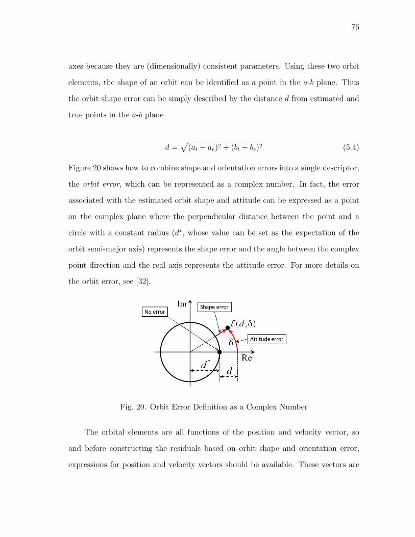
76
axes because they are (dimensionally) consistent parameters. Using these two orbit
elements, the shape of an orbit can be identified as a point in the a-b plane. Thus
the orbit shape error can be simply described by the distance d from estimated and
true points in the a-b plane
d =√
(at − ae)2 + (bt − be)2 (5.4)
Figure 20 shows how to combine shape and orientation errors into a single descriptor,
the orbit error, which can be represented as a complex number. In fact, the error
associated with the estimated orbit shape and attitude can be expressed as a point
on the complex plane where the perpendicular distance between the point and a
circle with a constant radius (d∗, whose value can be set as the expectation of the
orbit semi-major axis) represents the shape error and the angle between the complex
point direction and the real axis represents the attitude error. For more details on
the orbit error, see [32].
Fig. 20. Orbit Error Definition as a Complex Number
The orbital elements are all functions of the position and velocity vector, so
and before constructing the residuals based on orbit shape and orientation error,
expressions for position and velocity vectors should be available. These vectors are

77
simply given using the Lagrange interpolation polynomials. For the position vector
we have
r(t) = `1(t) r1 + `2(t) r2 + `3(t) r3 (5.5)
where the `i(t) coefficients are the Lagrange interpolation polynomials
`i(t) =∏k 6=i
t− tkti − tk
, i = 1, 2, · · · , 3 (5.6)
while for the velocity vector we have
v(t) = r(t) = ˙1(t) r1 + ˙
2(t) r2 + ˙3(t) r3 (5.7)
Equations (5.5) and (5.7) provide position and velocity vectors in terms of the un-
known ranges ρk, k = 1, 2, 3.
a. Residuals Based on Orbit Orientation Error.
The orbit orientation at the mid-range t = t2 (out of three observations) can now be
defined as cos δ21 =
1
2[tr(C T
21C2)− 1]
cos δ23 =1
2[tr(C T
23C2)− 1](5.8)
where C2 is the orbit orientation at t = t2, C21 and C23 are the orbit orientations
at t2 obtained by propagating and back-propagating to t2 from times t1 and t3,
respectively. The angles δ21 and δ23 are the orientation errors. Let us know rewrite
the orientation matrices in terms of position and angular momentum vectors as in
Eq. (5.9) C21 =
[r21, h21 × r21, h21
]TC23 =
[r23, h23 × r23, h23
]TC2 =
[r2, h2 × r2, h2
]T (5.9)

78
where r21 and r23 are the position vector directions propagated and back-propagated
to t2 from t1 and t3, respectively. We know that the orientation error angles (δ21 and
δ23) ideally should be zero resulting in the left hand side of Eq. (5.8) to be one; hence tr(C T21C2) = 3
tr(C T21C2) = 3
(5.10)
Let us now expand Eq. (5.10) in terms of the components of the orientation matrices
C2, C21, and C23, so we have r21 · r2 + t21 · t2 + h21 · h2 = 3
r23 · r2 + t23 · t2 + h23 · h2 = 3(5.11)
Equation (5.10) implies that to have the minimum orbit orientation error, the value
of each term in the parenthesis should be equal to one which makes perfect sense as
the error in minimum when r21, r23, h21, and h23 directions are pointing, respectively,
to the r2, r2, h2, and h2 directions. The terms involving t are redundant as t is
achieved from the cross product of h and r. So, now the residual associated with
the orbit orientation error can be constructed as ψr = σ−1r (r21 − r2)
ψh = σ−1h (h21 − h2)(5.12)
or as another set of the residual ψr = σ−1r (r23 − r2)
ψh = σ−1h (h23 − h2)(5.13)
The expressions for r21 and h21 in the first residual set (same trend for the second
set of residual) are obtained by propagating the initial position and velocity vectors

79
t = t1 to t = t2 as r21 = f1r1 + g1v1
h21 = r21 × v21 = (f1r1 + g1v1)× (f1r1 + g1v1)(5.14)
where f , g, f , and g are the Lagrange functions and their respective time derivatives.
For small time interval between the measurements (with respect to the orbit error),
the Lagrange functions are f1 ≈ 1− µ
2r314t2
g1 ≈ −4t+µ
6 r314t3
(5.15)
where ∆t is the time interval between the measured line-of-sights and µ is the grav-
itational constant. The angular momentum h21 can be expanded as
h21 = (f1g1 − f1g1)h1 (5.16)
In a Keplerian’s Two-body problem, the term f1g1 − f1g1 is equal to one, so h21
becomes h1. The residual for the orbit orientation error can be expressed in the
following form ψr = σ−1r [(f1r1 + g1v1)− r2]
ψh = σ−1h (h1 − h2)(5.17)
Note that the second equation of Eq. (5.17) is simply the conservation of angular
momentum.
b. Residuals Based on Orbit Shape Error
The orbit shape error can be defined as in Eq. (5.4) or simply in a residual force as ψa = σ−1a (a1 − a2)
ψe = σ−1e (e1 − e2)(5.18)

80
or as another set of residuals ψa = σ−1a (a3 − a2)
ψe = σ−1e (e3 − e2)(5.19)
Now we can define the whole set of residuals containing both orbit shape and orbit
orientation error as
ψ =
ψr
ψh
ψa
ψe
8×1
(5.20)
Writing Taylor’s series expansion
ψj+1∼= ψj +
[∂ψ
∂ρ
]j
4ρj +H.O.T. (5.21)
and the optimal solution can be written as
4ρj = −J†j ψj (5.22)
where index j denotes the j-th iteration. The solution in the update form
ρj+1 = ρj − J†j ψj (5.23)
and since J is not necessarily square, its pseudo inverse J† is obtained using Moore-
Penrose rule as
J† = (J TJ)−1 J T (5.24)
which leads to the final update form of
ρj+1 = ρj − (J T
j WJj)−1 J T
j Wψj, j = 1, 2, ..., n (5.25)
where W is a weight matrix. This algorithm has iterative nature, so an initial guess

81
is required to start the process. The iteration is performed until ∆ρj < ε where
ε is some predefined tolerance. Note that residual vector ψ is only a function of
the unknown range ρj, j = 1, 2, 3 as the semi-major axis a, eccentricity e, and
angular momentum h are all functions of position r and velocity v vectors and the
velocity vector is also can be expressed in terms of the unknown ranges ρj, j = 1, 2, 3
according to Eq. (5.7). So, the Jacobian J is just a function of ρj.
The authors refer to the new technique as Vn where “V ” stands for “variation”
as the method is based on the variation of orbital error and n is the number of
observations used for the initial orbit determination (e.g. V3, uses three observations).
C. Generalizing to Multiple Observations
This technique was originally developed with three observations, but it can easily be
generalized to multiple observations for enhanced performance and accuracy. Also,
for the coplanar orbit determination scenarios (it is when the measured line-of-sights
lie on the orbit plane), the classical and some of the newly developed initial orbit
determination methods show singularities. One remedy to bypass this draw back is
using one more observation. Consider that we have multiple n observations available.
The residuals (both orbit shape and orbit orientation) of each three observations can
be put in the form of Eq. (5.24), so for n measurements we have
ψ =ψT
r1,ψT
h1, ψa1 , ψe1 ,ψ
T
r2,ψT
h2, ψa2 , ψe2 , · · · ,ψT
rn ,ψT
hn , ψan , ψenT
(5.26)
where the vector ψ contains 8(n − 2) elements. The solution, ρk, k = 1, 2, · · · , n,
should be able to minimize the the residual ψ in Eq. (5.26). The rest of the procedure
is identical to that of three observations, Eq. (5.21) through (5.25). Note that the
82
Jacobian matrix J is defined as
J8(n−2)×n =
[∂ψi∂ρj
], i = 1, 2, · · · , 8(n− 2), j = 1, 2, · · · , n (5.27)
As seen in the forgoing, for three observations derivations, the velocity vectors were
approximated using Lagrange Interpolation Polynomials. As the number of obser-
vations increases, working with the Lagrange Interpolation polynomials gets more
complex and ineffective. To by pass this drawback, the least square scheme was
employed for velocity vector approximations which leads to more simplicity and of
course more accuracy. To this end, consider that the position vector components
(simply x, y, and z) can be approximated using the following N -th polynomialspx(t) = a1 + a2t+ a3t
2 + · · ·+ aN+1tN
py(t) = b1 + b2t+ b3t2 + · · ·+ bN+1t
N
pz(t) = c1 + c2t+ c3t2 + · · ·+ cN+1t
N
(5.28)
and consequently the velocity vector component can be approximately determined
as Vx(t) = px = a2 + a3t+ a4t
2 + · · ·+ aN+1tN−1
Vy(t) = py = b2 + b3t+ b4t2 + · · ·+ bN+1t
N−1
Vz(t) = pz = c2 + c3t+ c4t2 + · · ·+ cN+1t
N−1
(5.29)
For more details regarding how to implement the least square to obtain the velocity
vectors in terms of the unknown ranges, see [30]. In practice, not the full length
residual vector ψ is required to find the optimum solution. As a matter of fact, since
as the number of observations increases, the size of the residual vector grows much
faster, using the full length vector would result in convergence instability. So using
a portion of the residual vector not only yields more robustness and higher accuracy,
but less CPU time.
83
D. Selected Test Scenarios and Results
The validation of the developed technique was tested through several different sce-
narios. All the observations were made from a ground-based site located at a point
of zero longitude and zero latitude for the sake of simplicity. To simulate the real
data, the ideal measured data were corrupted with Gaussian noise with standard
deviation of 3σ = 10′′. To test the performance of the presented algorithms, Monte
Carlo analysis was conducted using 441 non-coplanar and 438 coplanar Low Earth
Orbit (LEO) different scenarios. A random orbit generator was used for the purpose.
For the non-coplanar cases, the orbits have the eccentricity ranging from 0 to 0.2,
inclination ranging from 5 to 90, and semi-major axis ranging from 6,786.352 km
to 9,424.253 km. The coplanar scenarios have the eccentricity ranging from 0 to 0.2
and semi-major axis ranging from 6,746.727 km to 9,731.184 km. Qualitative and
quantitative analysis was performed to have a better understanding of the perfor-
mance of the developed algorithm. For the Monte Carlo analysis, three different time
intervals were considered for both coplanar (∆t = 60, 80, 100 s) and non-coplanar
(∆t = 120, 150, 180 s) cases. For the non-coplanar, the estimated a and b with
relative percentage error up to 0.25% (defined as 100×|true− estimated|/true) and
δ (principal angle of the corrective matrix-error) up to 0.05 were collected as accept-
able performance. For the coplanar, the estimated a and b with relative percentage
error up to 0.5% and θ (angle between the angular momentum vectors) up to 0.05
were collected as acceptable performance. The results from Vn were compared to
that of the classical methods of Gauss and Laplace. Tables XIV and XV present the
results of the Monte Carlo analysis. For the Monte Carlo analysis, the number of
occurrences and corresponding percentage meeting the requirements are presented.
The method Vn is rather robust with respect to the initial guess as this technique is
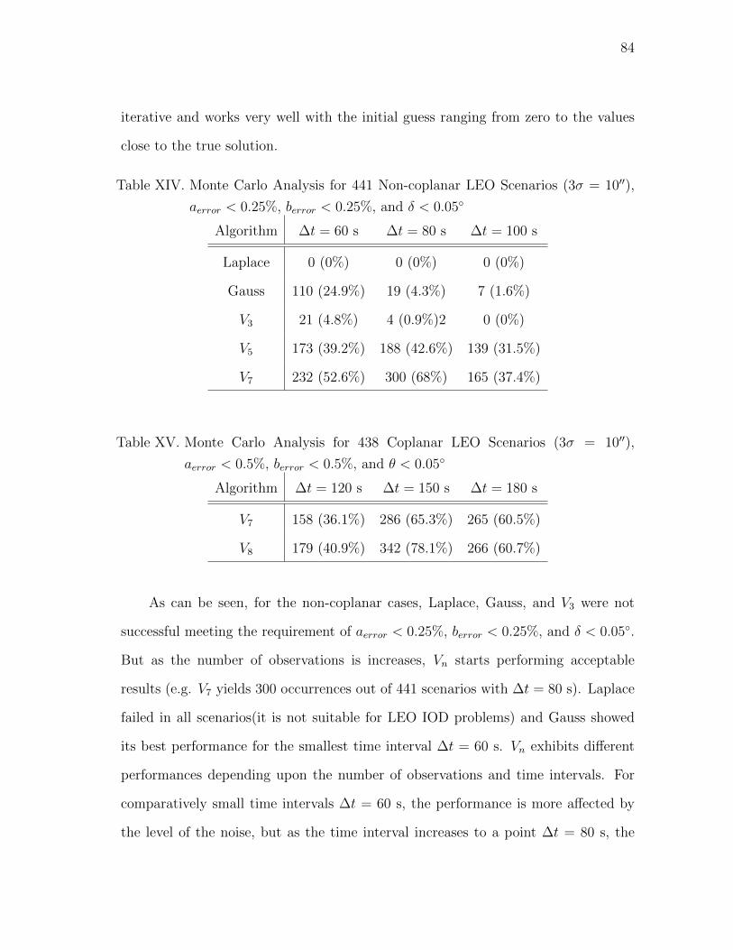
84
iterative and works very well with the initial guess ranging from zero to the values
close to the true solution.
Table XIV. Monte Carlo Analysis for 441 Non-coplanar LEO Scenarios (3σ = 10′′),
aerror < 0.25%, berror < 0.25%, and δ < 0.05
Algorithm ∆t = 60 s ∆t = 80 s ∆t = 100 s
Laplace 0 (0%) 0 (0%) 0 (0%)
Gauss 110 (24.9%) 19 (4.3%) 7 (1.6%)
V3 21 (4.8%) 4 (0.9%)2 0 (0%)
V5 173 (39.2%) 188 (42.6%) 139 (31.5%)
V7 232 (52.6%) 300 (68%) 165 (37.4%)
Table XV. Monte Carlo Analysis for 438 Coplanar LEO Scenarios (3σ = 10′′),
aerror < 0.5%, berror < 0.5%, and θ < 0.05
Algorithm ∆t = 120 s ∆t = 150 s ∆t = 180 s
V7 158 (36.1%) 286 (65.3%) 265 (60.5%)
V8 179 (40.9%) 342 (78.1%) 266 (60.7%)
As can be seen, for the non-coplanar cases, Laplace, Gauss, and V3 were not
successful meeting the requirement of aerror < 0.25%, berror < 0.25%, and δ < 0.05.
But as the number of observations is increases, Vn starts performing acceptable
results (e.g. V7 yields 300 occurrences out of 441 scenarios with ∆t = 80 s). Laplace
failed in all scenarios(it is not suitable for LEO IOD problems) and Gauss showed
its best performance for the smallest time interval ∆t = 60 s. Vn exhibits different
performances depending upon the number of observations and time intervals. For
comparatively small time intervals ∆t = 60 s, the performance is more affected by
the level of the noise, but as the time interval increases to a point ∆t = 80 s, the

85
results accuracy improves as the measured data are less affected by the level of noise,
but for larger time intervals ∆t = 100 s, the performance drops again regardless of
the level of the noise involved as the velocity approximation accuracy decreases. So,
there is an optimum combination of number of observation and time intervals. For
coplanar scenarios, Laplace, Gauss, and V3 failed. Coplanar cases are sensitive to
the level of noise involved in the measurements, so a larger time interval is required
compared to the case of non-coplanar. As can be seen from Table XV, the result id
achieved with V8 and ∆t = 150s. As the time interval decreases, the data get more
affected by the noise and as it increases, the velocity approximation accuracy drops,
so like for the non-coplanar cases, there is an optimum combination of number of
observations and time interval. Apart from this qualitative analysis, we also were
interested in testing some specific scenarios as quantitative comparison. So, one
random case was considered for each non-coplanar and coplanar with the level of
noise of 3σ = 10′′. The orbital elements of the non-coplanar and coplanar scenarios
are presented in Table XVI.
Table XVI. Orbital Elements for a Single Random Scenario
Scenario a e i Ω ω ϕ
km [-] (deg) (deg) (deg) (deg)
Non-coplanar 7,800.0 0.1 45 345 15 0
Coplanar 7,800.0 0.1 0 0 0 0
Tables XVII, XVIII, and XIX present the semi-major axis, semi-minor axis
relative percentage errors (orbit shape error), attitude error matrix principal angle
(orbit orientation error), position and velocity relative percentage errors for the non-
coplanar single case with ∆t = 60, 80, 100 s.
As can be seen, the best performance is yielded by V7 with ∆t = 60 s and as
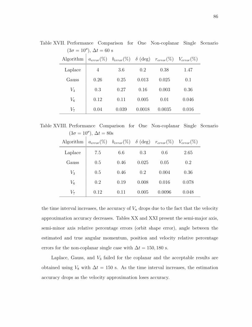
86
Table XVII. Performance Comparison for One Non-coplanar Single Scenario
(3σ = 10′′), ∆t = 60 s
Algorithm aerror(%) berror(%) δ (deg) rerror(%) Verror(%)
Laplace 4 3.6 0.2 0.38 1.47
Gauss 0.26 0.25 0.013 0.025 0.1
V3 0.3 0.27 0.16 0.003 0.36
V6 0.12 0.11 0.005 0.01 0.046
V7 0.04 0.039 0.0018 0.0035 0.016
Table XVIII. Performance Comparison for One Non-coplanar Single Scenario
(3σ = 10′′), ∆t = 80s
Algorithm aerror(%) berror(%) δ (deg) rerror(%) Verror(%)
Laplace 7.5 6.6 0.3 0.6 2.65
Gauss 0.5 0.46 0.025 0.05 0.2
V3 0.5 0.46 0.2 0.004 0.36
V6 0.2 0.19 0.008 0.016 0.078
V7 0.12 0.11 0.005 0.0096 0.048
the time interval increases, the accuracy of Vn drops due to the fact that the velocity
approximation accuracy decreases. Tables XX and XXI present the semi-major axis,
semi-minor axis relative percentage errors (orbit shape error), angle between the
estimated and true angular momentum, position and velocity relative percentage
errors for the non-coplanar single case with ∆t = 150, 180 s.
Laplace, Gauss, and V3 failed for the coplanar and the acceptable results are
obtained using V8 with ∆t = 150 s. As the time interval increases, the estimation
accuracy drops as the velocity approximation loses accuracy.

87
Table XIX. Performance Comparison for One Non-coplanar Single Scenario
(3σ = 10′′), ∆t = 100 s
Algorithm aerror(%) berror(%) δ (deg) rerror(%) Verror(%)
Laplace 11.9 10.3 0.5 0.8 4
Gauss 0.86 0.78 0.045 0.088 0.32
V3 0.77 0.7 0.27 0.015 0.65
V6 0.15 0.14 0.0062 0.012 0.056
V7 0.28 0.23 0.001 0.02 0.094
Table XX. Performance Comparison for One Coplanar Single Scenario (3σ = 10′′),
∆t = 150 s
Algorithm aerror(%) berror(%) θ (deg) rerror(%) Verror(%)
V7 0.31 0.28 0.001 0.008 0.12
V8 0.2 0.19 0.001 0.003 0.097
E. Conclusions
A novel technique of initial orbit determination based on the variation of orbital error
was developed and tested. The main idea of the method is based on the fact that,
for Keplerian orbits, the orbital elements, defining the orbital error, should remain
constant at any time. Different Monte Carlo analysis for both non-coplanar and
coplanar Low Earth Orbit scenarios were performed as a qualitative analysis with
various time intervals between the measurements. Also one single specific scenarios
for each non-coplanar and coplanar were tested as a quantitative analysis. The
estimated errors were presented in terms of orbit shape, orbit orientation errors, and
position and velocity relative percentage error. The results from Vn were compared to
those of the classical initial orbit determination methods of Gauss and Laplace. The

88
Table XXI. Performance Comparison for One Coplanar Single Scenario (3σ = 10′′),
∆t = 180 s
Algorithm aerror(%) berror(%) θ (deg) rerror(%) Verror(%)
V7 0.4 0.36 0.002 0.0078 0.167
V8 0.37 0.34 0.002 0.0039 0.165
best results were achieved using V7 and V8 for non-coplanar and coplanar scenarios
respectively. With small time intervals, the measurements are more affected by
the noise and as the time interval increases, the estimation accuracy improves to
some point and as the time interval continue growing, the performance drops mainly
because of the fact that the velocity approximation accuracy decreases. For number
of observations more than three, least square scheme was employed rather than
Lagrange interpolation functions to approximate the velocity which leaded to less
complex derivations/coding and higher accuracy. For the coplanar case, Laplace,
Gauss, and V3 failed whereas V8 with ∆t = 150 s showed the most acceptable result.
The coplanar cases are sensitive to the level of noise involved in the measurements,
so to avoid convergence instability, a larger time interval compared to a non-coplanar
case should be selected. The method Vn is rather robust with respect to the initial
guess as this technique is iterative and works very well with the initial guess ranging
from zero to the values close to the true solution. The orbit shape and orientation
error residuals used in this analysis had a vector form. Different types of residual/cost
functions should be tried and tested.

89
CHAPTER VI
SPACE-BASED INITIAL ORBIT DETERMINATION
In this chapter, the performance of the developed techniques are tested through two
different space-based initial orbit determination scenarios. The first scenario is a Low
Earth Orbit-to-Low Earth Orbit (LEO-to-LEO) problem and the satellites Iridium33
and Cosmos 2251 which collided into each other on February 10, 2009 is considered
as the case study. The second scenario is a LEO-to-GEO (Geosynchronous) case.
A. Challenges of Space-based IOD versus Ground-based IOD
As seen in the foregoing sections, the initial orbit determination problems under
study were all ground-based, with a stationary observing site, whereas in space-based
case, the observer is an orbiting object itself. The fact that the known observer has
a velocity with a magnitude compared to that of the unknown observed orbiting
object, poses a problem. As a result, the measured lines-of-sight are more effected
by the noise and this makes the problem of space-based orbit determination more
challenging versus the ground-based scenarios. A technique to lessen the effect of
the noise on the measured data is presented.
1. Satellite Conjunction
The collision of two satellites on February 10, 2009, Iridium-33 and Cosmos-2251,
has generated a renewed interest in collision detection and avoidance. The recent
collision occurred 789 km above northern Siberia, a location where no current obser-
vation stations exist. Current methods of optical and radar tracking and high-fidelity
propagation obviously failed in this case as post collision analysis showed that the
collision could have been avoided. This paper presents a novel method of collision
90
detection and avoidance based on in-orbit orbit determination.
The problem statement for this work is as follows: from a satellite with known
orbit parameters, can we estimate the orbit parameters of an unknown object (e.g.,
satellite) using an on-board optical system–like a star tracker–and then determine if
(or where) the satellites collide?
An accurate estimate of the orbit of the approaching object is required to be
able to avoid the collision. The known satellite plays the role of an observer trying
to track and determine the orbit of the unknown approaching one, the unknown.
Methods Pn and Jn were used for the purpose.
Example problems are solved to validate the orbit determination technique being
capable of handling a collision avoidance problem. According to ESA-MASTER
2001, the highest spatial density of space debris belongs to the orbits with altitude
of almost 1000 km. The examples studied in this paper will have an altitude of
the LEO satellites around 1000 km. The problems were also solved with different
number of observations and time intervals between the measurements to come up
with the optimum number of measurements-time intervals with respect to accuracy
and processor running time, as time plays a significant role in a collision avoidance
problem.
2. Problem Description
Figure 21 shows a schematic of a potential satellite collision problem. Satellite 1 has
a known orbit and is the observer. It is tracking satellite 2, the target, which has an
unknown orbit and poses a potential threat to the observer. Once the position and
velocity vectors of the target are determined through the initial orbit determination
(IOD) technique explained in the next section, the orbital elements of the unknown
approaching object can be determined. Points P1 and P2 are the respective perigees,
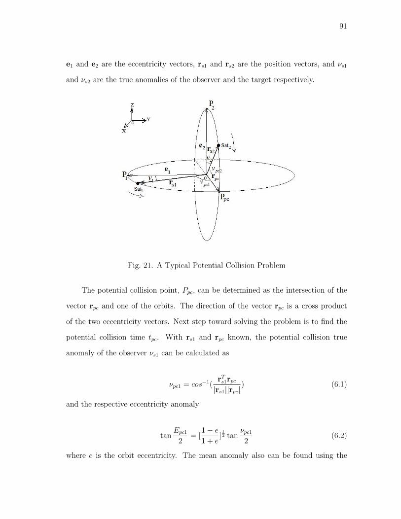
91
e1 and e2 are the eccentricity vectors, rs1 and rs2 are the position vectors, and νs1
and νs2 are the true anomalies of the observer and the target respectively.
Fig. 21. A Typical Potential Collision Problem
The potential collision point, Ppc, can be determined as the intersection of the
vector rpc and one of the orbits. The direction of the vector rpc is a cross product
of the two eccentricity vectors. Next step toward solving the problem is to find the
potential collision time tpc. With rs1 and rpc known, the potential collision true
anomaly of the observer νs1 can be calculated as
νpc1 = cos−1(rTs1rpc|rs1||rpc|
) (6.1)
and the respective eccentricity anomaly
tanEpc1
2= [
1− e1 + e
]12 tan
νpc12
(6.2)
where e is the orbit eccentricity. The mean anomaly also can be found using the
92
Kepler’s equation
Mpc1 = Epc1 − e sinEpc1 (6.3)
and finally the potential collision time tpc can be determined as
tpc =Mpc1
n1
(6.4)
where n1 is the mean motion of the observer satellite. Next, the last position vector
of the target, rs2, is propagated as determined by the observer. Having done this, the
resultant position vector would be rpc2, the potential collision position vector of the
approaching object. Note that rpc1 is the same as rpc whose direction was calculated
as the cross product of e1 and e2. The last step is now to apply the collision criterion
as
|rpc − rpc2| < ε⇒ COLLISION (6.5)
where ε is the radius of a ball within which collision occurs. To have a higher accuracy,
the observer needs to keep on measuring the line-of-sights from the unknown object
as it is approaching the observer to correct the previous data. Also the observer
needs to have enough time so in the case of predicted collision the observer is able
to perform an avoidance maneuver.
3. Noise Effect Reduction
The noise involved in the measurements (typically up to few arcsecs for conventional
star-trackers) plays a significant role in the performance of the IOD methods and has
a big impact on the accuracy of the estimated orbit parameters. So a technique to
reduce the effect of the noise seems to be vital for the orbit determination problems.
93
The scheme that was developed in this work is based on the concept of curve-fitting.
The measured direction ρi, i = 1, 2, ...n can be written in a component form as
ρxi =
1
ρi(rxi −Rx
i )
ρyi =1
ρi(ryi −R
yi )
ρzi =1
ρi(rzi −Rz
i )
(6.6)
The behavior of the measured directions components ρxi , ρyi ,and ρzi then can be
approximated by a fitting curve well representing the behavior of the noise-less data.
For the purpose of the current work, a second order polynomial exhibited the best
fit. More details will be presented in the Simulation section.
Figure 22 shows a simulated actual orbit (blue), the unfiltered noisy data (green),
and the filtered estimate (red). As can be seen from the figure, the filtering process
greatly improves the accuracy of the estimates.
4. Simulation and Results
To test the performance of the proposed techniques, three space-based initial orbit
determination scenarios were considered. The first one is a LEO-to-LEO case with
orbits similar to the Iridium-33 and Cosmos-2251 spacecraft (some tweaking was
done to ensure collision for the simulation). The initial orbital elements used for
the simulation are shown in Table XXII and the orbits are shown in Figure 23 (the
spacecraft representing Iridium is shown in blue while the spacecraft representing
Cosmos is shown in red). The second case, is a LEO-to-GEO case in in which a low
earth orbit spacecraft is trying to estimate the orbit of a Geosynchronous satellite,
and the the last is a GEO-to-GEO case (Geosynchronous observing Geosynchronous).

94
Fig. 22. Measured Directions: True, Noisy, and Filtered
a. LEO-to-LEO (Iridium 33-Cosmos 2251 Scenario)
Due to the spacecraft both being in low Earth orbit (LEO), the maximum possible
observation range between the two (without interference from the Earth’s limbs)
was about 6300 km. Methods Jn and Pn exhibited acceptable performance and
methods Ln, Vn, and MLn did not yield applicable results. The observations are
made before the collision for various times of collision tc ranging from 1200s to
400s.Three different time intervals ∆ = 20, 40, 60s are considered for Jn and two time
intervals ∆t = 80, 100s for Pn. The two techniques showed their best performances
with different number of observations. While Jn required ten observations Nobs = 10
to show its acceptable performance, Pn used eight. The level of noise involved in
the measurements has a standard deviation of 3σ = 10”. Since we are dealing
with a satellite conjunction detection and avoidance problem, two things should be
95
Table XXII. Orbital Elements of Satellites for Simulation
Orbital Element Target Spacecraft Value Observer Spacecraft Value
a (km) 7187.3 7161.2
e 0.00337 0.00056
i (deg) 74.04 86.38
ω (deg) 136.89 261.48
Ω (deg) 71.16 51.13
M (deg) 223.45 98.85
considered: a) The last observation should be made early enough before the potential
conjunction so that the satellite has time to perform an evasive manoeuver, and b)
after the initial obit determination is done, the estimated position and velocity should
be propagated for the purpose of collision detection, so to evaluate the estimation
accuracy of Jn and Pn, the set rerror and verror should be considered together. Tables
XXIII, XXIV, and XXV show the results of Jn and Tables XXVI and XXVII show
those of Pn. The orbital elements of the target satellite (Cosmos) are presented and
since the orbit of Cosmos is near circular, the sum of argument of perigee and true
anomaly is considered (e.g. θ = ω+ϕ). Also the estimation error is presented in the
form of relative percentage error.
As can be seen, the best (rerror,verror) sets using Jn are (0.07%, 0.71%), tc = 600s,
(0.08%, 0.65%), tc = 400s, (0.027%, 1.28%), tc = 1200s, and (0.063%, 0.82%), tc =
1000s, and the best (rerror,verror) sets using Pn are (0.058%, 0.77%), tc = 1000s and
(0.086%, 0.71%), tc = 1000s. Note that in the set where rerror% has the lowest value
of 0.027, verror% has the maximum value of 1.28. Besides, the potential conjunction
time tc is 1200s, while the set (rerror,verror)=(0.08%, 0.65%) has a higher position and
almost same order velocity error compared to the previous set, but the potential col-

96
Fig. 23. Orbits of the Simulated Spacecrafts
lision time is 400s. So, the error propagation possibly is not as much as the previous
case. Since the subject of error propagation and satellite conjunction detection and
avoidance is beyond the scope of this dissertation, the interested reader is referred
to [38]. Method Pn typically requires larger time intervals to yield accuracies equal
to or better than Jn. The shortest time interval used for Pn was ∆ = 80s that is 20s
longer than the largest time interval of Jn which is 60s.
b. LEO-to-GEO (Coplanar)
In this scenario, a low earth orbit satellite is observing an unknown geosynchronous
orbiting object. To make the problem more challenging, the orbits were considered
circular and coplanar. The orbital elements of both satellites can be found in Table
XXVIII.
The best results were achieved using methods Jn, Ln, and Pn. Three time
intervals ∆ = 900, 1200, 1800s were considered with Nobs = 8, and the noise involved
has a standard deviation of 3σ = 10”. The errors are presented in terms of shape

97
Table XXIII. Iridium33 - Cosmos2251 Scenario Using Jn, Nobs = 10, ∆t = 20s,
3σ = 10”
tc (s) aerr(%) berr(%) ierr(%) Ωerr(%) (ω + ϕ)err(%) rerr(%) Verr(%)
1200 0.249 0.249 0.63 1 0.049 0.14 1.5
1000 0.25 0.25 0.28 0.79 0.035 0.11 1
800 0.25 0.25 0.071 0.66 0.03 0.088 0.85
600 0.18 0.18 0.043 0.4 0.018 0.07 0.71
400 0.1 0.1 0.11 0.18 0.0097 0.08 0.65
Table XXIV. Iridium33 - Cosmos2251 Scenario Using Jn, Nobs = 10, ∆t = 40s,
3σ = 10”
tc (s) aerr(%) berr(%) ierr(%) Ωerr(%) (ω + ϕ)err(%) rerr(%) Verr(%)
1200 0.3 0.3 0.37 0.96 0.044 0.027 1.28
1000 0.27 0.27 0.067 0.67 0.03 0.063 0.82
800 0.2 0.2 0.12 0.38 0.02 0.147 0.47
600 0.033 0.033 0.22 0.063 0.004 0.3 0.13
error (semi-major and semi-minor axis) and since the orbits are coplanar, the angle
between the angular momentum vectors θ is considered as the orientation error.
Tables XXIX, XXX, and XXXI present the results.
As can be seen, all three methods show superb performance and specifically Ln
with ∆t = 1200s for shape error and with ∆t = 1800s for orientation and position
and velocity errors. One reason could be due to the fact that Ln is capable of using
more terms of Lagrange coefficients f and g;hence, more accurate results compared
to Jn. Also note that Pn is based on polynomial approximations.

98
Table XXV. Iridium33 - Cosmos2251 Scenario Using Jn, Nobs = 10, ∆t = 60s,
3σ = 10”
tc (s) aerr(%) berr(%) ierr(%) Ωerr(%) (ω + ϕ)err(%) rerr(%) Verr(%)
1200 0.348 0.348 0.048 0.83 0.04 0.16 1
1000 0.254 0.254 0.237 0.425 0.025 0.32 0.51
800 0.052 0.052 0.426 0.148 0.0078 0.59 0.084
Table XXVI. Iridium33 - Cosmos2251 Scenario Using Pn, Nobs = 8, ∆t = 80s,
3σ = 10”
tc (s) aerr(%) berr(%) ierr(%) Ωerr(%) (ω + ϕ)err(%) rerr(%) Verr(%)
1200 0.31 0.31 0.24 0.86 0.035 0.14 1
1000 0.27 0.27 0.01 0.63 0.026 0.058 0.77
c. GEO-to-GEO
In this scenario, a geosynchronous satellite is trying to determine the orbit of another
GEO spacecraft. This scenario is the most challenging one as far as the angles-only
initial orbit determination is concerned. This case has observability issue and almost
all available IOD methods are not capable of fully handling the problem. The space-
based orbit determination cases in which the distance between the observer and
target (range) is small, also suffer from observability issues. The results of GEO-to-
GEO will not be presented in this dissertation as requested by the Space Engineering
Research Center (SERC), Texas A&M University.
5. Conclusion
The performance of the angles-only initial orbit determination algorithms developed
in this work were tested for three specific different space-based IOD scenarios, namely
LEO-to-LEO (Iridium 33 - Cosmos 2251 case), LEO-to-GEO, and GEO-to-GEO.

99
Table XXVII. Iridium33 - Cosmos2251 Scenario Using Pn, Nobs = 8, ∆t = 100s,
3σ = 10”
tc (s) aerr(%) berr(%) ierr(%) Ωerr(%) (ω + ϕ)err(%) rerr(%) Verr(%)
1200 0.34 0.34 0.12 0.85 0.033 0.16 1
1000 0.28 0.28 0.11 0.57 0.36 0.086 0.71
Table XXVIII. Orbital Elements of LEO-GEO Scenario (Circular and Coplanar Or-
bits)
Orbital Element LEO Satellite GEO Target
a (km) 10,000.0 42,164.137
e 0 0
i (deg) 0 0
ω (deg) 0 0
Ω (deg) 0 0
ϕ (deg) 0 1.5
The methods Pn and Jn showed acceptable results for the Iridium 33 - Cosmos 2251
problem. A collision occurred between the satellites Iridium 33 and Cosmos 2251
on Feb.10, 2009 and the main reason behind selecting this case was find out if the
conjunction could have been detected and avoided. Different number of observations
and time intervals were tested among which Jn with Nobs = 10, ∆ = 20s and potential
collision time tc of 400s seemed to have the highest accuracy for the purpose. Also
if the orbit determination is performed too late, the observer satellite may not have
enough time to perform an evasive manoeuver, or have to apply a large amount ∆V
which may not be feasible due to the energy limitations on board spacecraft. For
the LEO-to-GEO case, the methods Pn, Jn, and Ln showed excellent results. The
obits were considered circular and coplanar to challenge the proposed algorithms.

100
Table XXIX. LEO-to-GEO Scenario, (Circular and Coplanar), Nobs = 8, ∆t = 900s,
3σ = 10”
Method aerr(%) berr(%) θ(Deg) rerr(%) verr(%)
Pn 0.0013 0.0013 0.041 0.0039 0.079
Jn 0.0028 0.0028 0.0077 0.0057 0.041
Ln 0.0013 0.0013 0.0077 0.0048 0.03
Table XXX. LEO-to-GEO Scenario, (Circular and Coplanar), Nobs = 8, ∆t = 1200s,
3σ = 10”
Method aerr(%) berr(%) θ(Deg) rerr(%) verr(%)
Pn 0.00117 0.00117 0.029 0.0041 0.054
Jn 0.0169 0.0169 0.005 0.0042 0.041
Ln 0.00032 0.00032 0.0056 0.00389 0.0178
The number of observations Nobs = 8 with different time intervals were used among
which the technique Ln with ∆t = 1200s yielded the most accurate orbit shape and
with ∆t = 1800s showed the most accurate orientation and position and velocity
estimation. And finally, the GEO-to-GEO case which because of the sensitivity of
the material, the results were not included.

101
Table XXXI. LEO-to-GEO Scenario, (Circular and Coplanar), Nobs = 8, ∆t = 1800s,
3σ = 10”
Method aerr(%) berr(%) θ(Deg) rerr(%) verr(%)
Pn 0.0012 0.0012 0.015 0.0043 0.03
Jn 0.016 0.016 0.0031 0.02 0.19
Ln 0.00075 0.00075 0.003 0.0037 0.012

102
CHAPTER VII
DESIGNING AN INTERPLANETARY AUTONOMOUS SPACECRAFT
NAVIGATION SYSTEM USING VISIBLE PLANETS
In this chapter, the design of an interplanetary autonomous spacecraft navigation
system is presented. The first section discuses the challenges of an interplanetary
spacecraft navigation problem. Second two explains how to implement the correc-
tions need to be made to the initial orbit determination method to make it suitable
for the spacecraft navigation scenario. Then, Extended Kalman Filter is briefly ex-
plained and applied as the autonomous navigation system. Finally, the results and
conclusion are presented. This chapter is the continuation of [39].
A. Challenges of an Interplanetary Spacecraft Navigation Problem
An interplanetary mission is a voyage through space involving more than one planet.
Mariner 2 was the first successful interplanetary spacecraft flying past Venus in 1962.
Mars exploration began with Mariner 4 in 1965. Since then, all the planets except
Pluto have been visited by interplanetary spacecrafts. In every interplanetary mis-
sion, the navigation plays a significant role in the success of the mission. Spacecraft
navigation comprises two aspects: (1) knowledge and prediction of spacecraft posi-
tion and velocity, which is orbit determination, and (2) firing the rocket motor to
alter the spacecraft’s velocity, which is flight path control. The current work focuses
on the first aspect of the spacecraft navigation. Duality exists between the problem
of orbit determination from line-of-sight measurements and the problem of an inter-
planetary autonomous navigation system. Both problems want to estimate an orbit.
So basically, in an interplanetary navigation problem, we are dealing with an space-
based orbit determination. There are challenges associated with an interplanetary

103
spacecraft navigation problem which makes it different from a typical space-based
orbit determination scenario. So, corrections need to be make to the orbit determina-
tion algorithms to make them applicable for the purpose. In the following subsection,
the corrections are described.
Corrections
In an Interplanetary spacecraft navigation problem, because of large distances be-
tween the orbiting objects and also the high speed of the observer (spacecraft) com-
pared to the ground-based case, two issues rise which need care, namely light-time
effect and relativistic aberration effects. These two phenomena are big sources of
error in the measured lines-of-sight. So apart from the measurement noise which
is dependent on the quality of the star treks, we are dealing with other sources of
measurement noise. In the following, the techniques through which the light-time
effect and stellar aberration including restricted relativistic aberration effect can be
corrected are described.
a. Light-time Correction
Light-time correction is a displacement in the apparent position of a celestial object
from its true position (or geometric position) caused by the object’s motion during
the time it takes its light to reach an observer, see [40],[41] for more on light-time
correction. The effect of finite light speed starts playing a role in the accuracy of
the solution ρj, j = 1, 2, ..., Nobs as we are dealing with more distant objects than
earth-orbiting satellites, specifically an interplanetary mission. For example, it takes
light several minutes to reach a typical spacecraft traveling in space (for instance
between Mars and Jupiter) and is observing Earth for navigation. Assume that the
observations are made at times tk, k = 1, 2, · · · , n with the respective measured

104
directions, ρk, k = 1, 2, · · · , n. Since the spacecraft does not have any knowledge
of how far it is from the Sun and correspondingly from the Earth (but it knows the
planet it is observing is Earth),so the known position vectors of the planet, Rk, and
the measured directions, ρk, k = 1, 2, · · · , n, will be considered the ones at times
tk, k = 1, 2, · · · , n while these belong to the time tk − δtk where δtk is the time that
takes light to reach the spacecraft.
To fix this problem, a modification in the algorithm needs to be made. The first
step would be determining the δt as
δtk =ρ∗kc
(7.1)
where c is the speed of light.
The next step would be updating the planet position vector as
Rupdated = R(tk − δtk) (7.2)
The position vector can be updated using Eq. (7.1) and Eq. (7.2). This process is
repeated until the desired accuracy is achieved.
b. Stellar Aberration Including Restricted (Special) Relativistic Effect
Relativistic aberration is described by Einstein’s special theory of relativity, and in
other relativistic models such as Newtonian emission theory. It results in aberration
of light when the relative motion of observer and light source changes the position
of the light source in the field of view of the observer. The effect is independent of
the distance between observer and light source.
The aberration of light (also referred to as astronomical aberration or stellar

105
aberration) is an astronomical phenomenon which produces an apparent motion of
celestial objects. At the instant of any observation of an object, the apparent position
of the object is displaced from its true position by an amount which depends upon
the transverse component of the velocity of the observer, with respect to the vector of
the incoming beam of light (i.e., the line actually taken by the light on its path to the
observer). Stellar aberration is independent of the distance of a celestial object from
the observer, and depends only on the observer’s instantaneous transverse velocity
with respect to the incoming light beam, at the moment of observation. The light
beam from a distant object cannot itself have any transverse velocity component, or
it could not (by definition) be seen by the observer, since it would miss the observer.
Thus, any transverse velocity of the emitting source plays no part in aberration.
Another way to state this is that the emitting object may have a transverse velocity
with respect to the observer, but any light beam emitted from it which reaches the
observer, cannot, for it must have been previously emitted in such a direction that its
transverse component has been “corrected” for. Such a beam must come “straight”
to the observer along a line which connects the observer with the position of the
object when it emitted the light [42]. In our problem, the light aberration is also
an issue which needs to be corrected. Assume that the angle between the spacecraft
velocity and the observed direction, ρobs, is θobs and the aberration angle (between
the true and observed directions) is ε, so the the corrected (true) planet observed
direction could be determined as
ρobs =v sin ε+ ρtrue sin θobs
sin θtrue(7.3)
where v is the spacecraft velocity unit vector and θtrue is the angle between the
velocity and true observation direction. The aberration angle ε, at any time, can be

106
Fig. 24. Light Aberration Caused by the Finite Speed of Light
obtained as
tan ε =(c/v)
√(1− (ρTobsv)2)
1− (c/v)(ρTobsv)=
(v/c) sin θobs1− (v/c) cos θobs
(7.4)
where c and v are the speed of light and spacecraft velocity magnitude respectively.
Note: The combination of light aberration and light-time correction is called plane-
tary aberration.
The relativistic aberration is basically the light aberration including the special
relativity. According to Einstein’s special relativity theory, light directions are af-
fected by the aberration toward inertial velocity vector. The apparent (observed)
and true light directions can be related as
cos θobs =cos θtrue + (v/c)
1 + (v/c) cos θtrue(7.5)
The apparent angle between the observed planet direction and spacecraft velocity
vector is known, and the true direction can be obtained using Eq. (7.5). This
ends the last modification we need to apply to the orbit determination (spacecraft
navigation) algorithm. Figure (24) illustrates the concept of stellar aberration. See
[43],[44] for more on relativistic aberration.

107
Fig. 25. Light-time and Stellar Aberration Including Restricted Relativistic Effect
Correction to the IOD Algorithm
Implementing the Corrections to the IOD Algorithm
The following flowchart Fig.(25) illustrates how the light-time and relativistic aber-
ration corrections are implemented into the initial orbit determination algorithm
.
B. Extended Kalman Filter Implementation
Up to now, we’ve developed some modifications through which an initial orbit deter-
mination technique can be applied to an interplanetary orbit determination scenario.
To have an autonomous navigation system, we need to perform a sequential state

108
estimation so we can have the real-time position and velocity of the space craft. To
this end, the Extended Kalman Filter (EKF) is employed as the estimation problem
under study involves nonlinear model. Considering a continuous-time truth nonlinear
model and discrete-time measurement, we have
x(t) = f(x(t),u(t), t) +G(t)w(t)
yk = h(xk) + νk
(7.6)
where x is the system state vector, y is the measurement, f is the system, u is the
input control, and G is the model error. And also, v and w are zero-mean Gaussian
white-noise processes meaning that the errors are not correlated forward or backward
in time. Their covariances are given by
EνkνTj =
0, k 6= j
Rk, k 6= j(7.7)
and
Ew(t)wT (τ) = Q(t)δ(t− τ) (7.8)
and since ν and w are uncorrelated
EνkwT (tk) = 0 (7.9)
A summary of the continuous-discrete Extended Kalman Filter is given in Table
XXXII.
where x(t) is the state estimate error, Kk is Kalman gain matrix at time tk, and
P (t) = Ex(t)xT (t) is the covariance of the state estimate error.
Now let us apply the Extended Kalman Filter to our problem. The system

109
Table XXXII. Continuous-discrete Extended Kalman Filter
Model x(t) = f(x(t),u(t), t) +G(t)w(t), w(t) ∼ N(0, Q(t))
yk = h(xk) + νk, νk ∼ N(0, Rk)
Initialize x(t0) = x0
P0 = Ex(t0)xT (t0)
Gain Kk = P−k HTk (x−k )[Hk(x
−k )P−k H
Tk (x−k ) +Rk]
−1
Hk(x−k ) ≡ ∂h
∂x|x−
k
Update x+k = x−k +Kk[yk − h(x−k )]
P+k = [I −KkHk(x
−k )]P−k
Propagation ˙x(t) = f(x(t),u(t), t)
P (t) = F (x(t), t)P (t) + P (t)F T (x(t), t) +G(t)Q(t)GT (t)
F (x(t), t) ≡ ∂f
∂x|x(t)
under study is well known and the truth model is available. For the space craft
traveling in the solar system under the Sun gravitational field, the motion is governed
by Keplerian two-body equations. Note that no perturbations (solar pressure and
gravity from other celestial bodies) are considered in this formulation, so we have
r = −µr3
r (7.10)
or in Cartesian form
x = −µ
r3x
y = −µr3y
z = −µr3z
(7.11)
where µ is the Sun Gravitational constant and r is the space craft position vector.
Defining the state vector X as
110
X1 = x
X2 = y
X3 = z
X4 = X1 = x
X5 = X2 = y
X6 = X3 = z
(7.12)
and the system dynamic would be
X = f(X(t)) =
x
y
z
− µ(x2 + y2 + z2)3/2
x
− µ(x2 + y2 + z2)3/2
y
− µ(x2 + y2 + z2)3/2
z
(7.13)
The input measurement vector y contains of azimuth φ and elevation θ angles as
illustrated in Fig.26.
y =
θ
φ
=
θ + νθ
φ+ νφ
(7.14)
where νθ and νφ are the measurement noise associated with the elevation and azimuth
angles respectively. The elevation and azimuth angles can be computed as
θ = sin−1[
(x−Rx)
[(x−Rx)2 + (y −Ry)2 + (z −Rz)2]1/2]
φ = tan−1[(y −Ry)
(x−Rx)]
(7.15)
For matrix H we have

111
Fig. 26. Azimuth and Elevation Angles as Input Measurements
H =∂h
∂X=
∂h1∂X1
∂h1∂X2
∂h1∂X3
∂h1∂X4
∂h1∂X5
∂h1∂X6
∂h2∂X1
∂h2∂X2
∂h2∂X3
∂h2∂X4
∂h2∂X5
∂h2∂X6
(7.16)
or
H =
∂θ
∂x
∂θ
∂y
∂θ
∂z0 0 0
∂φ
∂x
∂φ
∂y0 0 0 0
(7.17)
and components of matrix H

112
Fig. 27. Light-time and Stellar Aberration Including Restricted Relativistic Effect
Correction to EKF
∂θ
∂x= − (x−Rx)(z −Rz)
[(x−Rx)2 + (y −Ry)2 + (z −Rz)2][(x−Rx)2 + (y −Ry)2]1/2
∂θ
∂y= − (y −Ry)(z −Rz)
[(x−Rx)2 + (y −Ry)2 + (z −Rz)2][(x−Rx)2 + (y −Ry)2]1/2
∂θ
∂z= − [(x−Rx)
2 + (y −Ry)2]1/2
(x−Rx)2 + (y −Ry)2 + (z −Rz)2
∂φ
∂x= − y −Ry
(x−Rx)2 + (y −Ry)2
∂φ
∂y=
x−Rx
(x−Rx)2 + (y −Ry)2
(7.18)
Note that in the heart of the Extended Kalman Filter algorithm, the two corrections
of light-time and restricted relativistic light aberration are implemented. Figure (27)
illustrates how the light-time and stellar aberration relativistic aberration corrections
are implemented into EKF. For more details on extended Kalman filter, see [45].

113
C. Results
In this section the performance of the Autonomous Interplanetary Spacecraft Nav-
igation System Using Visible Planets is tested. The planet Earth is considered as
the known visible sun-orbiting object. A spacecraft is traveling on a trajectory with
an initial position of more than two hundred million kilometers from the Sun with
a distance of approximately seventy million kilometers from Earth (has almost the
same distance from Earth as Mars). The spacecraft is observing Earth for the nav-
igation purposes. The methods Pn, Jn, and Ln showed excellent performance for
the interplanetary space-based initial orbit determination part. Modified Laplace
MLn did not yield acceptable accuracy and Vn offered the trivial solution of almost
zero estimated ranges which is similar to the original Gooding method from this
aspect. Finally method Pn was selected for the IOD part (as the input to the ex-
tended Kalman filter) due to the fact that to make the special relativistic aberration
correction, the estimated velocities at each tk, k = 1, 2, ..., NNobs should be known
and method Pn computes those velocities in the heart of its algorithm and they are
already available as a part of the output and no need for extra computations as in
Ln and Jn. For the initial orbit determination part, the number of observations used
was Nobs = 8 with time interval ∆t = 3(105)s (3 days 11 hr 20 min). To make
the problem more challenging, the spacecraft orbit was considered coplanar with the
sun-earth orbit plane. Also note that the other planets have very small inclination
angles. The position and velocity components of the spacecraft and Earth at the
initial time t1 of observation are

114
rs/c=
−2
−0.5
0
108 km, vs/c=
2
−30
0
km/s, re=
−1.521
0
0
108 km, ve=
0
−29.29
0
km/s
The noise involved in the measurements has the standard deviation of 3σ = 10”.
The last (at t8) estimated position and velocity were used as the output of the
IOD algorithm and input to the Extended Kalman Filter. The state vector X0
(initial conditions for EKF) is defined as [rx, ry, rz, vx, vy, vz]T and for
this problem
X0 =
−183553246.154077
−129751886.849561
47.8566691563623
9.2804459659289
−26.6655452207945
0
For the Extended Kalman filter part, 150 observations with time interval ∆t =
3(103)s (50 min) were considered. For the navigation purpose,the estimated position
and velocity of the spacecraft are desired. No process noise was considered and
also we assumed the model has no error(no perturbations due to gravitational fields
of other planets and so solar pressure), so the covariance of the process noise q
was considered zero, q = 0. Also the initial values for P0 (covariance of the state
estimate error) was considered as P0 = 2(106)I6×6. Figures 28 and 29 show the
history of position and velocity error and the associated 3-σ bounds and the true
and estimated position and velocity respectively. The final estimated position and

115
Fig. 28. Estimated Position and Velocity Error with the 3-σ Bounds
velocity relative percentage error are rerror = 0.04% and Verror = 0.15% respectively.
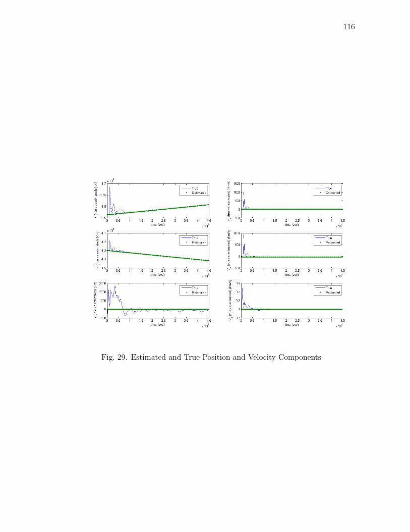
116
Fig. 29. Estimated and True Position and Velocity Components
117
D. Conclusion
An interplanetary autonomous spacecraft navigation system using visible planets was
designed and tested. Two corrections (light-time and light abberation) were made
to the space-based initial orbit determination algorithm to make it applicable for
an interplanetary spacecraft navigation problem. The output of the IOD method
(position and velocity) was used as the initial condition to Extended Kalman Filter
(EKF) for the autonomous estimation of the position and velocity of the spacecraft.
Planet Earth was used as the visible planet for the navigation purpose and the
spacecraft was traveling on a trajectory with a distance of approximately seventy
million kilometers from the planet(almost as the same distance as Mars). Of all
the five algorithms developed, Pn, Jn, Ln showed excellent performances for the
interplanetary angles-only initial orbit determination, but eventually Pn was chosen
for the autonomous navigation purpose as it was more comfortable to work with
when implementing the corrections of light-time and light abberation. For the initial
orbit determination, eight observations (Nobs = 8) was used with the time interval
of ∆t = 3(105)s (3 days 11 hr 20 min). The level of noise used to corrupt the
ideal data was considered as 3σ = 10”. For the autonomous navigation part, the
number of observations of 150 with ∆t = 3(103)s (50 min) were fed into the extended
Kalman filter.The final estimated position and velocity relative percentage error are
rerror = 0.04% and Verror = 0.15% respectively.

118
CHAPTER VIII
CONCLUSION
An interplanetary autonomous spacecraft navigation system using visible planets was
successfully designed and tested. The problem of interplanetary spacecraft naviga-
tion is the dual problem of the space-based angles-only Initial Orbit Determination
(IOD). The orbit determination methods can be used to solve the dual problem.
The classical and majority of newly developed angles-only IOD methods use three
lines-of-sight which pose the problem of singularity when used for the coplanar orbit
determination cases and also not efficient when employed for the space-based cases.
So, new tools were required to be built using which higher orbit estimation accu-
racy is achieved and also the issue of the singularity can be handled as the planets
have near to coplanar orbits. The techniques Jn, Ln, Pn, and MLn were developed
for the purpose. All five methods are capable of using multiple observations which
makes them suitable for the coplanar orbit determination problems. Also, using more
than three observations improve the estimation accuracy. The proposed algorithms
were tested for the ground-based, space-based (LEO-to-LEO and LEO-to-GEO) and
interplanetary (spacecraft-to-visible planet) initial orbit determination cases. For
the ground-based scenario, all five methods showed excellent performances for both
coplanar and non-coplanar cases. For the space-base (LEO-to-LEO, collision sce-
nario of Iridium 33 and Cosmos 2251 was considered as the case study), Pn and Jn
showed good performance. For the LEO-to-GEO, Pn,Jn, and Ln yielded excellent
results(a coplanar case was considered to make it more challenging). The methods
Vn and MLn showed their best performances for the ground-based orbit determina-
tion problems. To use the IOD method for the interplanetary spacecraft navigation
problem, two corrections needed to be made namely light-time (due to the large dis-
119
tance between the observer and observed objects and finite speed of light) and special
relativistic light aberration which causes the measured light-of-sight of the observed
planet to be compressed towards the velocity vector of the observer(spacecraft).
Also, to simulate the real world data, the ideal measured directions (lines-of-sight)
were corrupted with zero-mean Gaussian noise. For the interplanetary initial orbit
determination scenario, three techniques(Pn,Jn, and Ln) offered very well perfor-
mances. The output of the IOD method (position and velocity) was used as the
initial condition to Extended Kalman Filter (EKF) for the autonomous estimation
of the position and velocity of the spacecraft. Planet Earth was used as the visible
planet for the navigation purpose and the spacecraft was traveling on a trajectory
with a distance of approximately seventy million kilometers from the planet(almost
as the same distance as Mars). Out the three methods, Pn was eventually chosen
for the autonomous navigation purpose as it was more comfortable to work with
when implementing the corrections of light-time and light abberation. For the initial
orbit determination, eight observations (Nobs = 8) was used with the time interval of
∆t = 3(105)s (3 days 11 hr 20 min). The level of noise used to corrupt the ideal data
was considered as 3σ = 10”. For the autonomous navigation part, the number of
observations of 150 with ∆t = 3(103)s (50 min) were fed into the extended Kalman
filter. The estimated position and velocity of the spacecraft had relative percentage
errors of 0.04% and 0.15% respectively.
120
CHAPTER IX
FUTURE WORK
The designed autonomous spacecraft navigation system is tested experimentally and
the planet Earth will be considered as the spacecraft traveling in space while ob-
serving some other planet (could be Jupiter, Mars, or Venus) for navigation. Since
Earth has radius and is rotating, some modifications need to made as the original
algorithm considers the spacecraft as a point mass with no dimensions.
All the number of observations and time interval between the measurements were
chosen manually by the operator in such a way the estimation accuracy is achieved.
A smart scheme which can adaptively select the optimal number of observations and
time interval needs necessary. Such a work has already been started by the authors,
but still is at the early stages of development.
The method Vn yielded excellent performance for the ground-based initial orbit
determination whereas failed for the space-based case. The residual definitions should
be revised and different types of residual functions should be tested.
121
REFERENCES
[1] Green, R.M., Spherical Astronomy, Cambridge University Press, New York,
1988.
[2] Beer, A., and Strand, K.A., Copernicus, Pergamon Press, Oxford, UK, 1975.
[3] Vallado, D.A., Fundamental of Astrodynamics and Application, 3rd Ed., Micro-
cosm Press, Hawthorne, CA, 2007.
[4] Vetter, J.R., “Fifty Years of Orbit Determination: Development of Modern
Astrodynamics Methods,” Johns Hopkins APL Technical Digest , Vol. 27, No.
3, 2007, pp. 239–252.
[5] McClusky, S.C., Astronomies and Culture in Early Medical Early Europe, Cam-
bridge University Press, Cambridge, UK, 2000.
[6] Laplace, P.S., “Memoires de l’Academie Royale des Sciences,” Paris, Reprinted
in Laplace’s Collected Works, Vol. 10, No. 93, pp. 93–146, 1780.
[7] Gauss, C.F., Theory of the Motion of the Heavenly Bodies Moving about the Sun
in Conic Sections, English Translation, Dover Publication, New York, 1963.
[8] Anderson, J.D., “Theory of Orbit Determination. Part I: Classical Methods,” Jet
Propulsion Laboratory Technical Report, No. 32-497, Prepared Under Contract
No. NAS7-100, NASA, October 1963.
[9] Long, A.C., Goddard Trajectory Determination System (GTDS) Mathematical
Theory, Goddard Space Flight Center, Greenbelt, MD, 1989.
[10] Herget, P., “Determination of Orbits,” The Astronomical Journal, Vol. 44, No.
18, 1935, pp.153–161.

122
[11] Herget, P., The Computation of Orbits, Edwards Brothers, Inc., Ann Arbor,
MI, 1948.
[12] Escobal, P.R., Methods of Orbit Determination, John Wiley and Sons, Inc., New
York, 1965.
[13] Gooding, R.H., “A New Procedure for the Solution of the Classical Problem of
Minimal Orbit Determination from Three Lines of Sight,” Celestial Mechanics
and Dynamical Astronomy, Vol. 66, No. 4, 1997, pp. 387-423.
[14] Taff, L.G., “On Initial Orbit Determination,” The Astronomical Journal, Vol.
89, No. 9, 1984, pp.1426–1428.
[15] Gibbs, J.W., On the Detrmination of Elliptic Orbits from Three Complete Ob-
servations, Kessinger Publishing, Whitefish, Montana, 2008.
[16] Moulton, F.R., Celestial Mechanics, MacMillan, New York, 1902.
[17] Bate, R.R., Mueller, D.D., and White, J.E., Fundamental of Astrodynamics,
Dover Publications, New York, 1971.
[18] Herrick, S., Astrodynamics, Van Nostrand Reinhold Co., London, 1971.
[19] Battin, R.H., An Introduction to the Mathematics and Methods of Astrodynam-
ics, Education Series, AIAA, New York, 1987.
[20] Henderson, T.A., Mortari, D., and Davis, J., “Modifications to the Gooding Al-
gorithm For Angles-Only Initial Orbit Determination,” 2010 AAS/AIAA Space
Flight Mechanics Meeting Conference, San Diego, CA, Paper AAS 10-238, Feb.
2010.

123
[21] Celletti, A., and Pinzari, G., “Four Classical Methods For Determining Plan-
etary Elliptic Elements: A Comparision,” Celestial Mechanics and Dynamical
Astronomy, Vol. 93, No.1–4, 2005, pp.1–52.
[22] Shefer, V.A., “A Method of Intermediate Orbit Determination Based on Four
Positions of a Minor Body on the Celestial sphere,” Solar System Research, Vol.
42, No. 5, 2008, pp. 405-413.
[23] Taff, L.G., and Hall, D.L., “Use of Angles and Angular Rates in Initial Orbit
Determination,” Celectial Mechanics, Vol. 16, No. 4, 1977, pp. 481–488.
[24] Baker, R.M.L., Jr, and Jacoby, N.H., Jr, “Preliminary Orbit Determination
Method Having no Coplanar Singularity,” Celestial Mechanics, Vol. 15, No. 2,
1977, pp.137–160.
[25] Neutsch, W., “A Simple Method of Orbit Determination,” Astronomy and As-
trophysics, Vol. 102, No. 1, 1981, pp. 59–64.
[26] Kristensen, L.K., “Single Lunation N -Observation Orbits,” Celestial Mechanics
and Dynamical Astronomy, Vol. 105, No. 4, 2009, pp. 275–287.
[27] Karimi, R.R. and Mortari, D., “On Laplace’s Orbit Determination Method:
Some Modifications,” 2011 AAS/AIAA Space Flight Mechanics Meeting Con-
ference, New Orleans, LA, Paper AAS 11-121, Feb. 2011.
[28] Karimi, R.R. and Mortari, D., “On Preliminary Orbit Determination: A New
Approach,” 2009 AAS/AIAA Space Flight Mechanics Meeting Conference, Sa-
vannah, GA, Paper AAS 09-106, Feb. 2009.
[29] Karimi, R.R. and Mortari, D., “Initial Orbit Determination Using Multiple
Observations,” Celestial Mechanics and Dynamical Astronomy, Vol. 109, No. 2,

124
2010, pp.167-180.
[30] Karimi, R.R. and Mortari, D., “Orbit Determination Using Prescribed Orbits,”
2010 AAS/AIAA Space Flight Mechanics Meeting Conference, San Diego, CA,
Paper AAS 10-236, Feb. 2010.
[31] Karimi, R.R. and Mortari, D., “Orbit Determination Based on Variation of
Orbital Error,” 2012 AAS/AIAA Space Flight Mechanics Meeting Conference,
Charleston, SC, Paper AAS 12-201, Jan. 2012.
[32] Mortari, D., Scuro, R.S., and Bruccoleri, C. “Attitude and Orbit Error in n-
Dimensional Spaces,” AAS Journal of the Astronautical Sciences, Vol. 54, No.3–
4, 2006, pp. 467–484.
[33] Taff, L.G., Randall, P.M.S., and Stansfield, S.A., M.I.T. Lincoln Laboratory
Technical Report 618, May 1984.
[34] Curtis, H.D., Orbital Mechanics for Engineering Students, Elsevier Butterworth-
Heinemann, Oxford, UK, 2005.
[35] Turner, J.D., “Automated Generation of High-Order Partial Derivative Mod-
els,” AIAA Journal, Vol. 41, No. 8, 2003, pp. 1590–1598.
[36] Prussing, J.E. and Conway, B.A., Orbital Mechanics, Oxford University Press,
New York, 1993.
[37] Karimi, R.R., and Mortari, D., “An Adaptive Scheme on Optimal Number of
Observations and Time Intervals For An Iinitail Orbit Determination Problem,”
2010 AAS/AIAA Space Flight Mechanics Meeting Conference, San Diego, CA,
Paper AAS 10-152, Feb. 2010.

125
[38] Karimi, R.R., Henderson, T.A., and Mortari, D., “Satellite Collision Detection
and Avoidance using Star Trackers,” 2009 AAS/AIAA Astrodynamics Specialist
Conference, Pittsburgh, Pennsylvania, Paper AAS 09-302, Aug. 2009.
[39] Karimi, R.R. and Mortari, D., “Designing an Interplanetary Autonomous Space-
craft Navigation System Using Visible Planets,” 2009 AAS/AIAA Space Flight
Mechanics Meeting Conference, Savannah, GA, Paper AAS 09-160, Feb. 2009.
[40] Seidelmann, P.K., Explanatory Supplement to the Astronomical Almanac, Uni-
versity Science Books, Mill Valley, CA, 1992.
[41] Berry, A., A Short History of Astronomy, Dover Publications, Mineola, NY,
1961.
[42] Hirschfeld, A., Parallax: The Race to Measure the Cosmos, Henry Holt, New
York, 2001.
[43] Liebscher, D.E., and Brosche, P., “Aberration and Relativity,” Astronomische
Nachrrichten, Vol. 319, No. 5, 1998, pp.309–318.
[44] Gjurchinovski, A., “Aberration of Light in a Uniformly Moving Optical
Medium,” American Journal of Physics, Vol. 72, No. 7, 2004, pp. 934–940.
[45] Crassidis, J.L., and Junkins, J.L., Optimal Estimation of Dynamic Systems, 2nd
Ed., CRC Press, Boca Raton, FL, 2011.
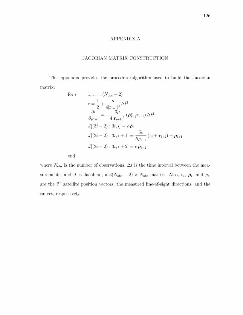
126
APPENDIX A
JACOBIAN MATRIX CONSTRUCTION
This appendix provides the procedure/algorithm used to build the Jacobian
matrix:
for i = 1, . . . , (Nobs − 2)
c =1
2+
µ
4|ri+1|3∆t2
∂c
∂ρi+1
= − 3µ
4|ri+1|5(ρT
i+1ri+1) ∆t2
J [(3i− 2) : 3i, i] = c ρi
J [(3i− 2) : 3i, i+ 1] =∂c
∂ρi+1
(ri + ri+2)− ρi+1
J [(3i− 2) : 3i, i+ 2] = c ρi+2
end
where Nobs is the number of observations, ∆t is the time interval between the mea-
surements, and J is Jacobian, a 3(Nobs − 2) × Nobs matrix. Also, ri, ρi, and ρi,
are the ith satellite position vectors, the measured line-of-sight directions, and the
ranges, respectively.

127
VITA
Reza Raymond Karimi graduated from Tehran Azad University with a B.S.
degree and from Tarbiat Modares University with a M.S. degree in Mechanical Engi-
neering. Reza migrated to the United Stated a year after his graduation and resided
in Texas. He attended Texas A&M University pursuing his PhD in Aerospace En-
gineering and graduated in May 2012. His areas of interests are Orbital Dynamics
with a focus on orbit determination and spacecraft navigation, nonlinear adaptive
control, real-time trajectory generation, and aircraft design. Reza will continue his
research as a postdoc and is seeking a research job in industry. He is the winner
of Lowy award for the best aircraft design, 2008 and outstanding graduate teaching
assistance award, 2007. He can be reached at [email protected] or in care
of Dr. Daniele Mortari at the Aerospace Engineering Department of Texas A&M
University, College Station, 77843-3141.