designguide,transient, momentum and the dacrmh072000/site/software_and_links_files/6a... ·...

1 ADS 2009 (version 1.0) Copyright Agilent Technologies 2009

DesignGuide,Transient, Momentum and the DAC


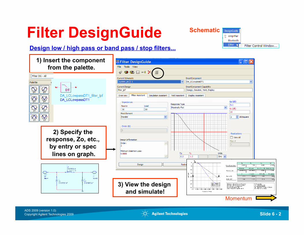
Filter DesignGuide Schematic

1) Insert the component from the palette.

2) Specify the response, Zo, etc., by entry or spec lines on graph.

3) View the design and simulate!

Momentum

Design low / high pass or band pass / stop filters...


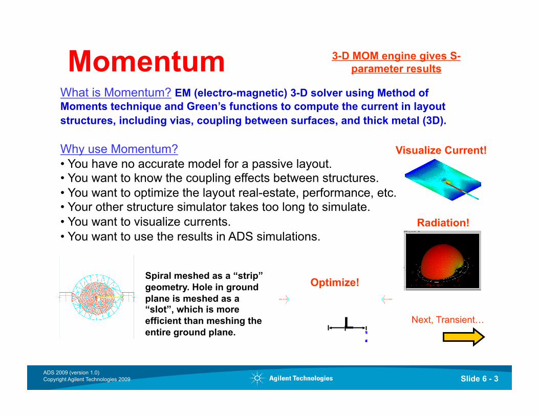
Momentum What is Momentum? EM (electro-magnetic) 3-D solver using Method of Moments technique and Green’s functions to compute the current in layout structures, including vias, coupling between surfaces, and thick metal (3D).

Why use Momentum? •  You have no accurate model for a passive layout. •  You want to know the coupling effects between structures. •  You want to optimize the layout real-estate, performance, etc. •  Your other structure simulator takes too long to simulate. •  You want to visualize currents. •  You want to use the results in ADS simulations.

Spiral meshed as a “strip” geometry. Hole in ground plane is meshed as a “slot”, which is more efficient than meshing the entire ground plane.

3-D MOM engine gives S-parameter results

Next, Transient… L

Optimize!

Visualize Current!

Radiation!


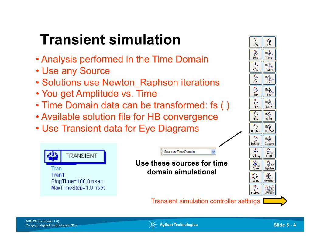
Transient simulation

Transient simulation controller settings

Use these sources for time domain simulations!


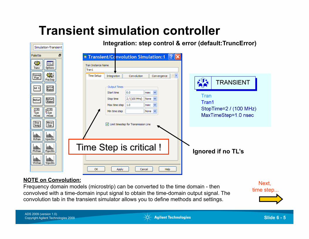
Transient simulation controller Integration: step control & error (default:TruncError)

Ignored if no TL’s

Next, time step...


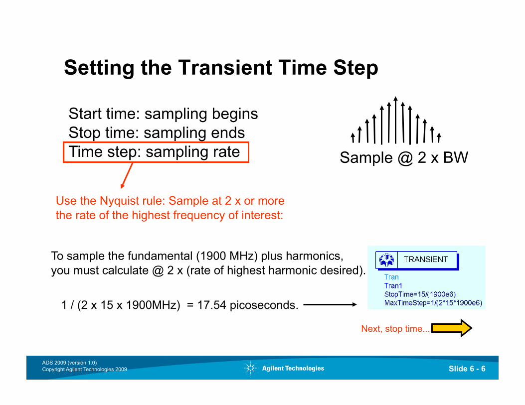
Setting the Transient Time Step

Use the Nyquist rule: Sample at 2 x or more the rate of the highest frequency of interest:

To sample the fundamental (1900 MHz) plus harmonics, you must calculate @ 2 x (rate of highest harmonic desired).

1 / (2 x 15 x 1900MHz) = 17.54 picoseconds.

Start time: sampling begins Stop time: sampling ends Time step: sampling rate Sample @ 2 x BW

Next, stop time...


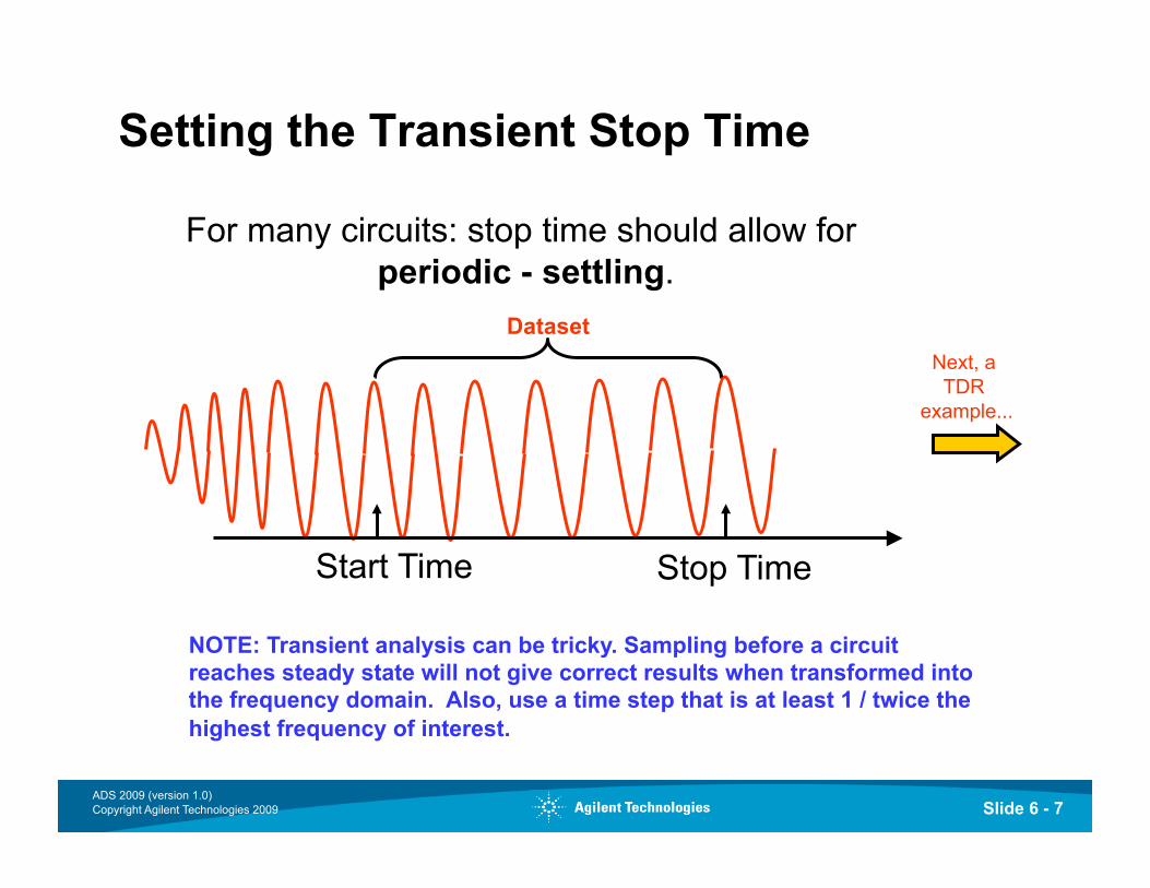
Setting the Transient Stop Time

For many circuits: stop time should allow for periodic - settling.

Stop Time Start Time

Dataset Next, a

TDR example...


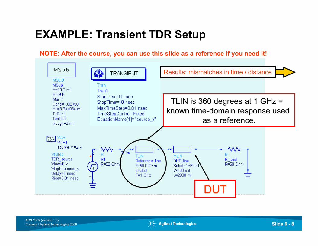
EXAMPLE: Transient TDR Setup NOTE: After the course, you can use this slide as a reference if you need it!

Results: mismatches in time / distance


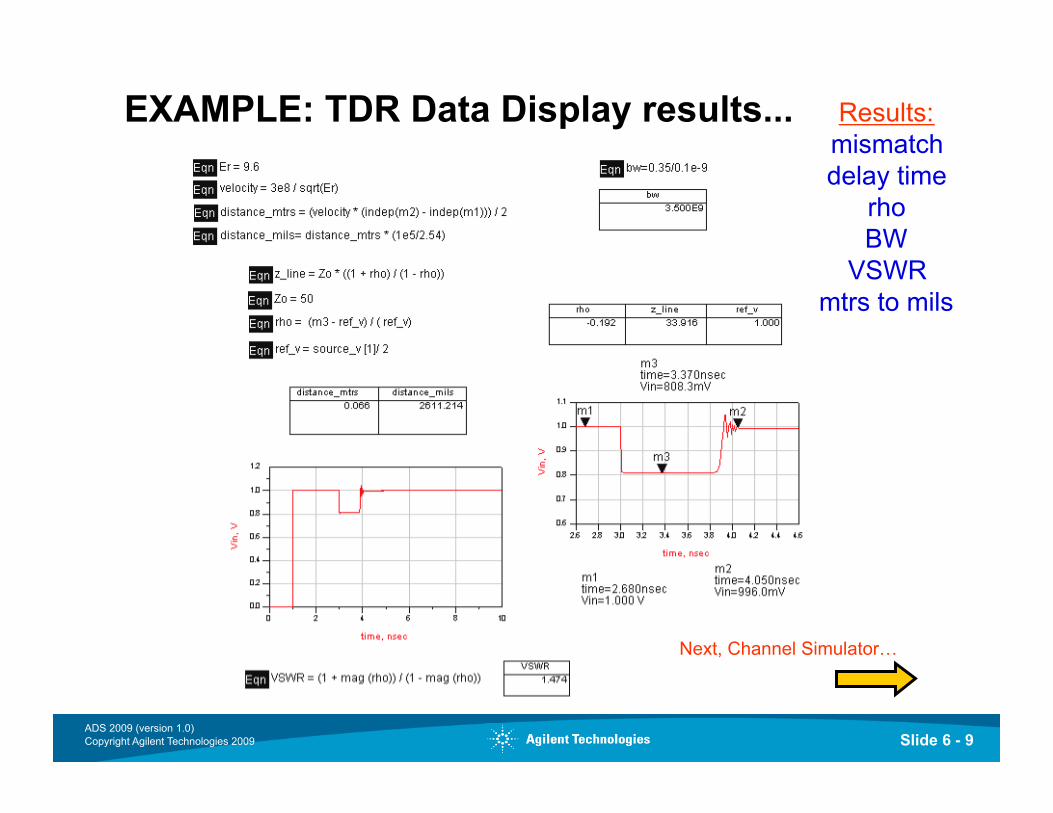
EXAMPLE: TDR Data Display results... Results: mismatch delay time

rho BW

VSWR mtrs to mils

Next, Channel Simulator…


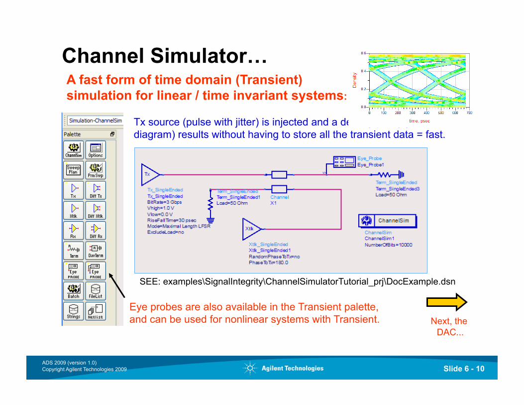
Channel Simulator…

Next, the DAC...

A fast form of time domain (Transient) simulation for linear / time invariant systems:

Eye probes are also available in the Transient palette, and can be used for nonlinear systems with Transient.

SEE: examples\SignalIntegrity\ChannelSimulatorTutorial_prj\DocExample.dsn

Tx source (pulse with jitter) is injected and a density plot (eye diagram) results without having to store all the transient data = fast.


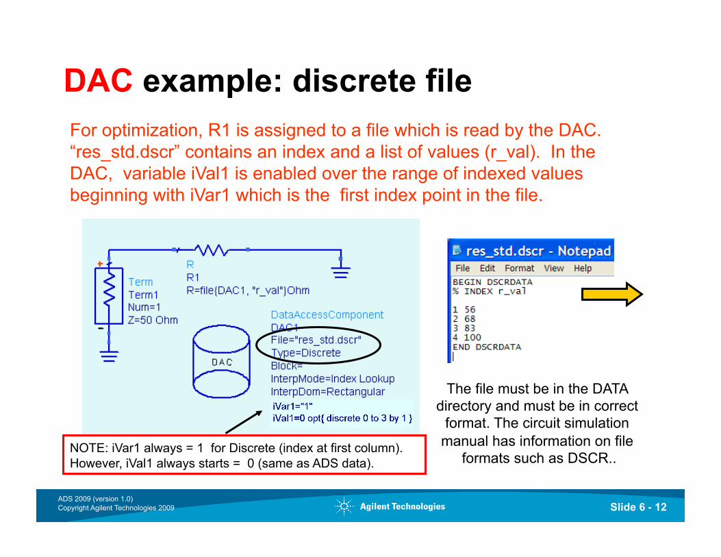
DAC (data access component)

File tab: Specify the file location, mode, edit, etc.

Independent Variable: Add vars, equations, etc.

NOTE: DACs are covered in detail in the Advanced class. DAC example:

The DAC points to a file and reads it: use for measured data or any tabular data.


DAC example: discrete file


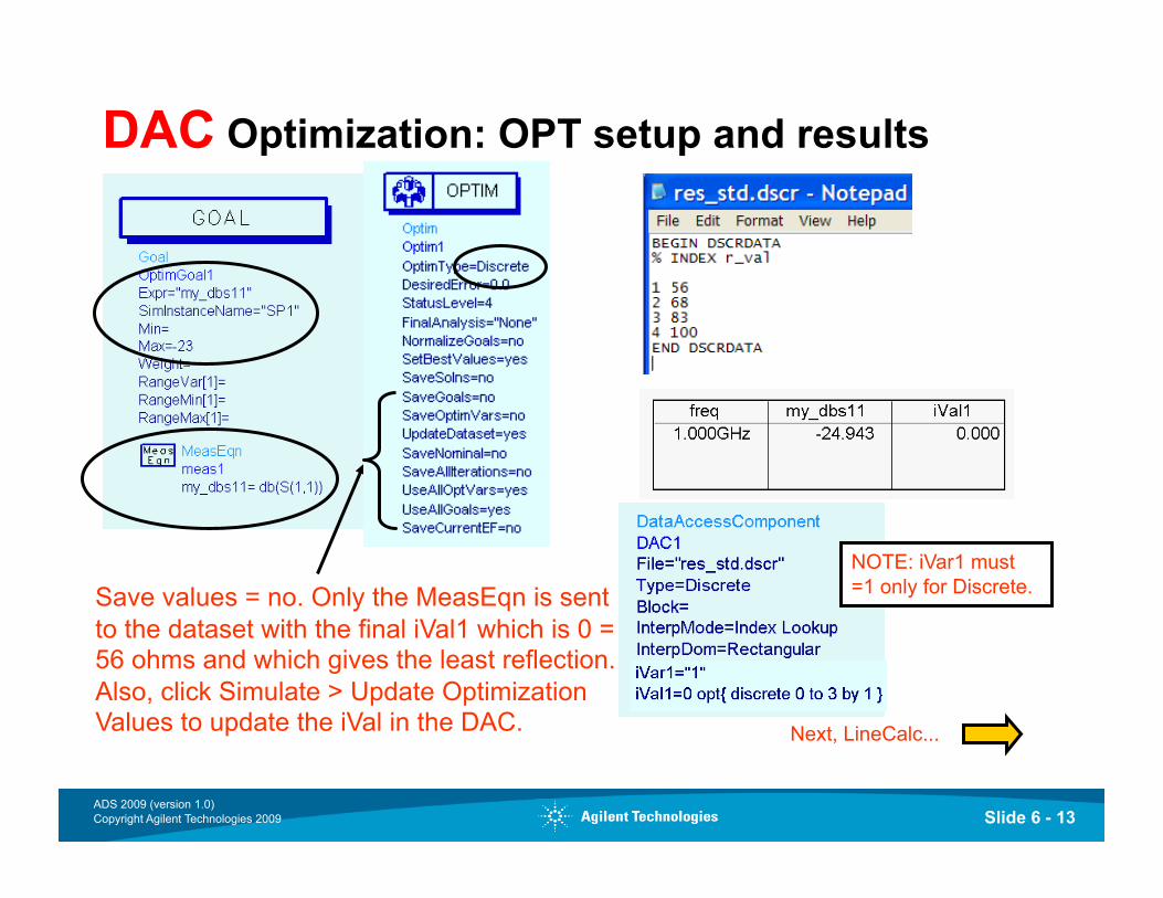
DAC Optimization: OPT setup and results

Save values = no. Only the MeasEqn is sent to the dataset with the final iVal1 which is 0 = 56 ohms and which gives the least reflection. Also, click Simulate > Update Optimization Values to update the iVal in the DAC. Next, LineCalc...

NOTE: iVar1 must =1 only for Discrete.


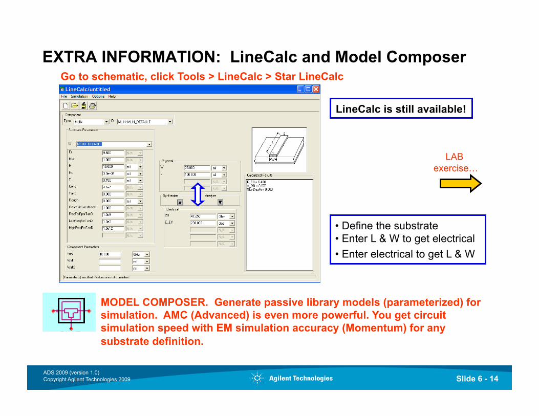
EXTRA INFORMATION: LineCalc and Model Composer

•  Define the substrate •  Enter L & W to get electrical •  Enter electrical to get L & W

Go to schematic, click Tools > LineCalc > Star LineCalc

MODEL COMPOSER. Generate passive library models (parameterized) for simulation. AMC (Advanced) is even more powerful. You get circuit simulation speed with EM simulation accuracy (Momentum) for any substrate definition.

LineCalc is still available!

LAB exercise…


Lab 6:

Filters: DesignGuide, Momentum, Transient

and the DAC


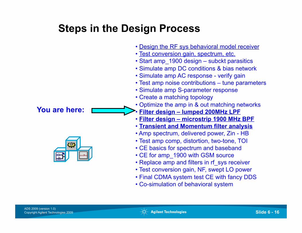
Steps in the Design Process •  Design the RF sys behavioral model receiver •  Test conversion gain, spectrum, etc. •  Start amp_1900 design – subckt parasitics •  Simulate amp DC conditions & bias network •  Simulate amp AC response - verify gain •  Test amp noise contributions – tune parameters •  Simulate amp S-parameter response •  Create a matching topology •  Optimize the amp in & out matching networks •  Filter design – lumped 200MHz LPF •  Filter design – microstrip 1900 MHz BPF •  Transient and Momentum filter analysis •  Amp spectrum, delivered power, Zin - HB •  Test amp comp, distortion, two-tone, TOI •  CE basics for spectrum and baseband •  CE for amp_1900 with GSM source •  Replace amp and filters in rf_sys receiver •  Test conversion gain, NF, swept LO power •  Final CDMA system test CE with fancy DDS •  Co-simulation of behavioral system

You are here:


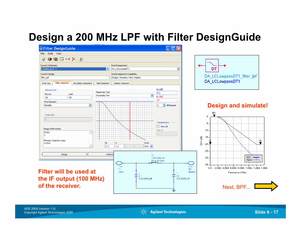
Design a 200 MHz LPF with Filter DesignGuide

Filter will be used at the IF output (100 MHz) of the receiver.

Design and simulate!

Next, BPF...


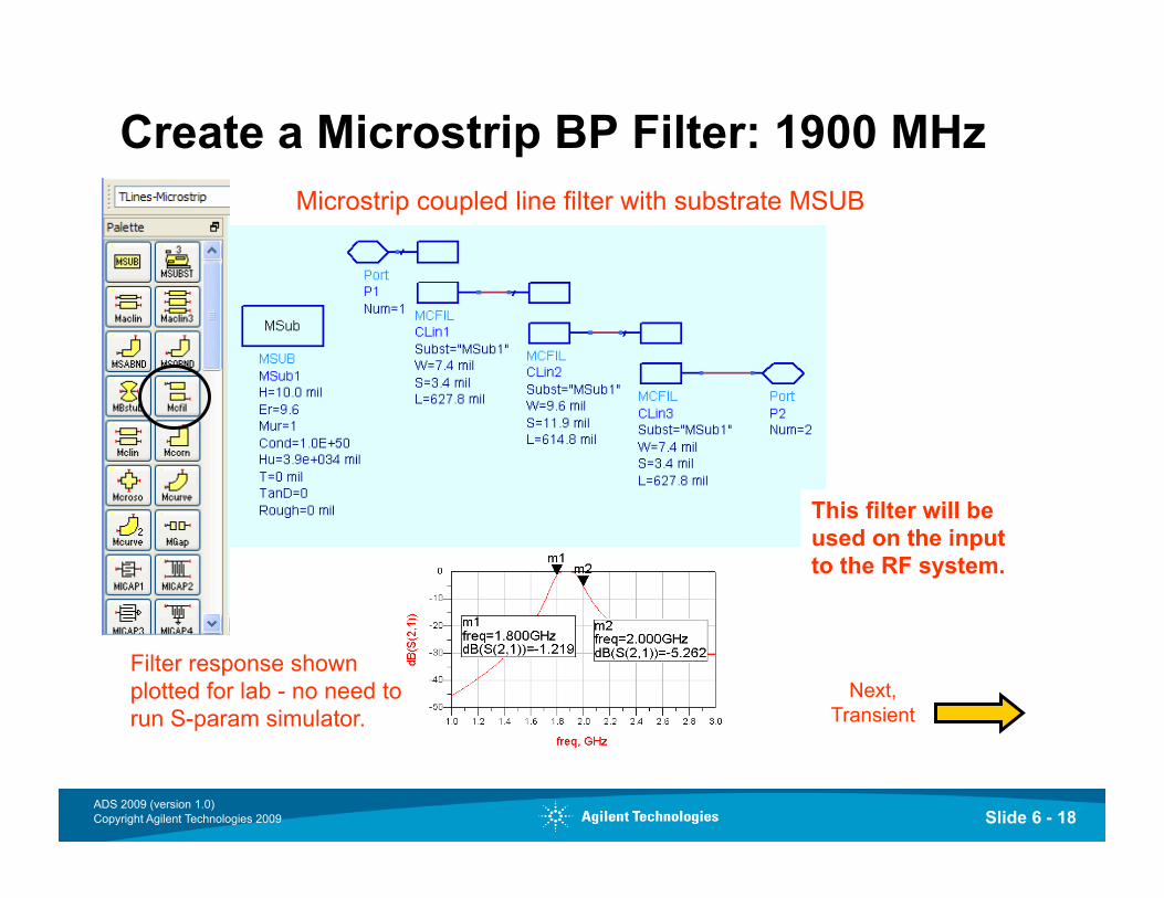
Create a Microstrip BP Filter: 1900 MHz Microstrip coupled line filter with substrate MSUB

Filter response shown plotted for lab - no need to run S-param simulator.

Next, Transient

This filter will be used on the input to the RF system.


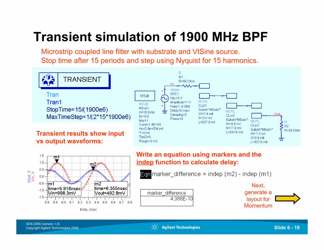
Transient simulation of 1900 MHz BPF Microstrip coupled line filter with substrate and VtSine source. Stop time after 15 periods and step using Nyquist for 15 harmonics.

Transient results show input vs output waveforms:

Write an equation using markers and the indep function to calculate delay:

Next, generate a layout for

Momentum


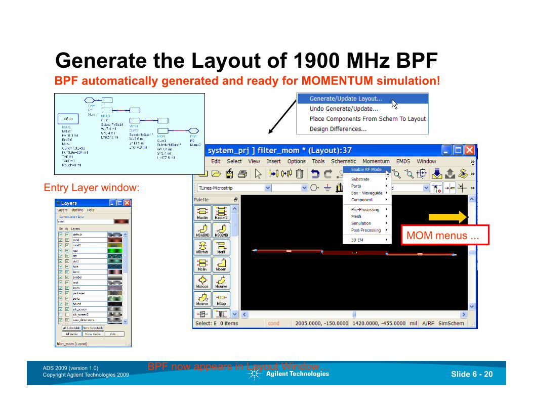
Generate the Layout of 1900 MHz BPF BPF automatically generated and ready for MOMENTUM simulation!

MOM menus ...

BPF now appears in Layout Window…

Entry Layer window:


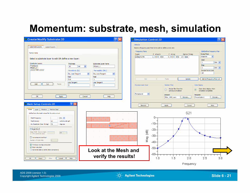
Momentum: substrate, mesh, simulation

Look at the Mesh and verify the results!


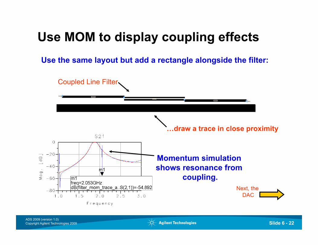
Use MOM to display coupling effects

Coupled Line Filter

…draw a trace in close proximity

Momentum simulation shows resonance from

coupling.

Use the same layout but add a rectangle alongside the filter:

Next, the DAC


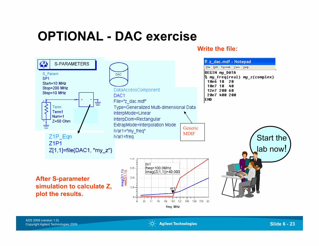
OPTIONAL - DAC exercise

After S-parameter simulation to calculate Z, plot the results.

Write the file:

Start the lab now!

Generic MDIF

designguide,transient, momentum and the dacrmh072000/site/software_and_links_files/6a... ·...

Documents