design study of a 250mev superconducting...

Design study of a 250MeV superconducting isochronous cyclotron for proton therapy

秦斌 (Bin QIN) for Particle Accelerator Group

State Key Laboratory of Advanced Electromagnetic Engineering and Technology, Huazhong University of Science and Technology

August 2014, SAP 2014, Lanzhou

OUTLINE

p Motivation & schemes comparison

p Design study

p Conclusions

Motivation

p The cancer is a leading cause of death worldwide. According to WHO's report, the number of new cancer cases and deaths will reach 15 million and 10 million in 2020; In China, 6.6 million and 3 million respectively

p In China, the survival and cure rate for cancer patients is about 12%;

p Compared to X-ray, gamma-ray, and electron beams, Proton therapy is the most effective method in radiation therapy,

u Minimum damage to healthy tissues surrounding at the target tumor, due to its unique ‘Bragg peak’ of dose distribution;

u  27 proton therapy centers located in worldwide, more than 50,000 patients treated, cure rate higher than 80%

!

Protons, electrons, X-ray and Gamma-ray （60Co）for cancer therapy

Dose distribution of proton beams 质子 X 射线

眼睛

鼻窦

颅骨

正常脑组织

脑干

低剂量高剂量

脑瘤脑瘤Tumor

质子 x 射线

Ø  For X-rays generated by linacs, absorbed dose, exponential decrease after initial peak (only 1/3 dose reached 20-25cm)

Ø  For proton beams, location of Bragg peak can be modulated by proton energy precisely

Proton therapy centers world wide

Ø  27 centers, 50000 patients treated；

Ø  Europe: 12, USA: 6, Japan: 5;

Ø  Synchrotron 7; Cyclotron 17; Synchro-cyclotron 3

A smooth conversion from a physics laboratory to a hospitalfacility took place in Japan. The University of Tsukuba startedproton clinical studies in 1983 using a synchrotron built

for physics studies at the High Energy Accelerator ResearchOrganization (KEK). A total of 700 patients were treated at thisfacility from 1983 to 2000. In 2000, a new in-house facility, called

Table 2Hospital based proton therapy facilities in operation at the end of 2008 [17].

Centre Country Acc. Max. clinical energy (MeV) Beam directiona Start of treat. Total treated patients Date of total

ITEP, Moscow Russia S 250 H 1969 4024 Dec-07St. Petersburg Russia SC 1000 H 1975 1327 Dec-07PSI, Villigenb Switzerland C 72 H 1984 5076 Dec-08Dubnac Russia SC 200 H 1999 489 Dec-08Uppsala Sweden C 200 H 1989 929 Dec-08Clatterbridgeb England C 62 H 1989 1803 Dec-08Loma Linda USA S 250 3G, H 1990 13,500 Dec-08Niceb France C 65 H 1991 3690 Dec-08Orsayd France SC 200 H 1991 4497 Dec-08iThemba Labs South Africa C 200 H 1993 503 Dec-08MPRI(2) USA C 200 H 2004 632 Dec-08UCSFb USA C 60 H 1994 1113 Dec-08TRIUMF, Vancouver b Canada C 72 H 1995 137 Dec-08PSI, Villigen e Switzerland C 250 G 1996 426 Dec-08HZB (HMI), Berlinb Germany C 72 H 1998 1227 Dec-08NCC, Kashiwa Japan C 235 2G, H 1998 607 Dec-08HIBMC, Hyogo Japan S 230 2G, H 2001 2033 Dec-08PMRC(2), Tsukuba Japan S 250 2G, H 2001 1367 Dec-08NPTC, MGH, Boston USA C 235 2G, H 2001 3515 Oct-08INFN-LNS, Cataniab Italy C 60 H 2002 151 Dec-07Shizuoka Japan S 235 2G, H 2003 692 Dec-08WERC,Tsuruga Japan S 200 H, V 2002 56 Dec-08WPTC, Zibo China C 230 3G, H 2004 767 Dec-08MD Anderson Cancer Centre, Houston, TXf USA S 250 3G, H 2006 1000 Dec-08FPTI, Jacksonville, FL USA C 230 3G, H 2006 988 Dec-08NCC, IIsan South Korea C 230 2G, H 2007 330 Dec-08RPTC, Munich g Germany C 250 4G, H 2009 Treatments started Mar-09TOTAL 50,879

a Horizontal (H), vertical (V), gantry (G).b Ocular tumours only.c Degraded beam.d 3676 ocular tumours.e Degraded beam for 1996–2006; dedicated 250 MeV proton beam from 2007. Scanning beam only.f With spread and scanning beams (since 2008).g Scanning beam only.

Fig. 2. The heart of the proton therapy facility of the Loma Linda University Medical Centre is a 7 m diameter synchrotron built by Fermilab. The protons are accelerated upto 250 MeV. Three gantry rooms and one room with horizontal beams are used.

U. Amaldi et al. / Nuclear Instruments and Methods in Physics Research A 620 (2010) 563–577 567

Courtesy of U. Amaldi et al., Nucl. Instru. Meth A, 620 (2010) 563

Planned Proton/Carbon Therapy Center

Ø  For new proton therapy centers, energy covers 210MeV-250MeV

(>25cm penetration depth), all adopt (superconducting) cyclotrons;

Ø  Carbon ions (C126+) , more heavy, more effective for radio-resistant

tumors; 25cm penetration depth requires 400MeV/u energy (magnetic

rigidity ~ 1.2GeV proton) à synchrotrons adopted for most cases;

In Japan, Y. Hirao and collaborators proposed the realization ofthe Heavy Ion Medical Accelerator in Chiba (HIMAC) to be built inthe Chiba prefecture. In 1994 the facility treated the first patientwith carbon ions at a maximum energy of 400 MeV/u,corresponding to a maximum range of 27 cm in water.

By the end of 2009, under the leadership of Hirohito Tsujii,about 5000 patients have been treated and many difficult andcommon tumours have been shown to be controllable [22]. Thedistribution of the range of carbon ion beams used at Chiba isshown in Fig. 4.

In 1993, Gerhard Kraft obtained the approval for theconstruction of a carbon ion facility at GSI (Darmstadt), latercalled the ‘pilot project’ [23]. Treatments started in 1997 andsince then about 400 patients have been treated with carbon ionbeams. There are four novel features of the GSI pilot project:

(i) the active ‘raster’ scanning system;(ii) the fully automatic control of the GSI accelerator complex,

that can be handled by an operator trained for standard X-rayequipment;

(iii) the sophisticated models and codes that take into accountthe RBE of different tissues in the treatment planning system;

(iv) the two gamma ray detectors placed above and below thepatient to determine ‘on-line’ the exact location and shape ofthe irradiated volume by means of the detection of 511 keVback-to-back photon pairs from positron annihilation. Thistechnique, named ‘in-beam-PET’ [24], is based on the factthat, when penetrating the body, some of the incident carbonions fragment into b+ radioactive nuclei, mainly 11C.

Hadrontherapy is now expanding very rapidly and severalhospital based facilities will be operational in the next years, asreported in Table 3. This list is necessarily incomplete due to thecontinuously increasing number of projects, which nowadayscharacterize this very active field of application of particle physicsto medicine.

4. Future developments of hadrontherapy techniques

Present hadrontherapy techniques have to be improved tofully exploit the unique spatial and biological advantages ofproton and ion beams. Even without major novelties, there isample space for improvements. In particular, it has to beremarked that ‘active’ dose delivery systems – based on scanned

pencil beams – have been used for less than 2% of the about60,000 patients treated with protons or ions. All the other patientshave been treated with wide beams shaped in the transversedimensions and in energy by sophisticated sets of passive devicessuch as scatterers, absorbers and collimators [25]. More advancedapproaches, still based on passive devices, have been developed inJapan: the ‘layer stacking’ technique [26] and the most recent‘cone type filter’ method [27].

In spite of the fact that most new centres have the possibilityof going from these ‘passive’ methods to ‘active’ systems, theimplementation in the clinical practice has been quite slow. Sinceequipment for active scanning is nowadays commercially avail-able, significant improvements in the quality of the dosedistribution systems are foreseen in the near future.

Looking further ahead, it has to be noted that, for protontherapy, the challenge is greater than for carbon ions. In the last10 years, the introduction of new X-ray delivery techniques hasimproved significantly the conformity of the dose distributions,with which proton treatments have to be naturally compared,since – within 10% – X-rays and protons have the sameradiobiological effects. Indeed, more and more hospitals introduceIntensity Modulated Radiation Therapy (IMRT) which uses manycrossed X-ray beams with optimized not uniform intensitydistributions produced by computer controlled ‘multi-leaf’collimators [15]. Tomotherapy [28] and Rapid Arc technologies[29] are novel developments now routinely used in manyradiation therapy departments. Moreover, the recent develop-ment of Image Guided Radiation Therapy (IGRT) [30][31] allows theon-line localization of tumour targets, which move duringirradiation due, for instance, to the inspiration–expiration cycle.

The irradiation of moving tumours is surely one of the mainchallenges hadrontherapy is facing. To effectively accomplish thistask, important technological developments are needed in thefields of

1. systems to actively scan in three dimensions with a pencilbeam tumours which are subject to movements;

2. devices which can detect the instantaneous position of thetumour target and produce signals to be used in a feedbackloop connected with the systems of point 1;

3. instruments capable of continuously monitoring the distribu-tion of the dose in the body of the patient;

4. in-beam PET devices allowing the range determination of theproton and ion beams at the end of an irradiation by detecting

Table 3Proposed new hadrontherapy facilities.

Location Country Particle Max. energy (MeV) - Acc. Beams a Rooms Foreseen start date

University of Pennsylvania USA p 230 cyclotron 4G, 1H 5 2009PSI, Villigen Switzerland p 250 SC cyclotron 1G additional to 1G, 1 H 3 2009 (OPTIS2), 2010 (Gantry2 )WPE, Essen Germany p 230 cyclotron 3G, 1H 4 2009HIT, Heidelberg Germany p, C 430/u synchrotron 1G for C ions, 2H 3 2009CPO, Orsay France p 230 cyclotron 1G additional to 2H 3 2010CNAO, Pavia Italy p, C 430/u synchrotron 2H, 1 H+V 3 2010PTZ, Marburg Germany p, C 430/u synchrotron 3H, 1 OB 4 2010NIPTRC, Chicago USA p 250 SC cyclotron 2G, 2H 1H (research) 4 2011NRoCK, Kiel Germany p, C 430/u synchrotron 1H, 1V+OB, 1H+V 3 2012Trento Italy p 230 cyclotron 1G, 1H 2 2012Skandionkliniken, Uppsala Sweden p 250 SC cyclotron 2G, 1H 3 2013Med-AUSTRON, Wiener Neustadt Austria p, C 400/u synchrotron 1G (p only), 1V, 1V+OB 3 2013Shanghai China p, C 430/u synchrotron 1H, 1V+OB, 1H+V 3 ?iThemba Labs South Africa p 230 cyclotron 1G, 2H 3 ?RPTC, Koeln Germany p 250 SC cyclotron 4G, 1H 5 ?ETOILE, Lyon France p, C ? ? ? ?

a Horizontal (H), 901 vertical (V), 451 oblique (OB), rotating gantry (G).

U. Amaldi et al. / Nuclear Instruments and Methods in Physics Research A 620 (2010) 563–577 569

Courtesy of U. Amaldi et al., Nucl. Instru. Meth A, 620 (2010) 563

R&D of hadron therapy facilities in China

•  Shanghai Proton therapy facility, proposal by Prof. FANG Shouxian et al., (IHEP, SINAP), Synchrotron scheme (2009)

•  R&D initiated in CIAE, Synchrocyclotron scheme

•  For carbon therapy, IMP (Lanzhou) HIRFL-CSR has performed experiments on shallow-seated tumors (104 cases, 2006-2009) and deep-seated tumors (110 cases, 2009-2013); new carbon therapy centers at Lanzhou & Wuwei are under-constructed

•  Initial stage for proton therapy facilities

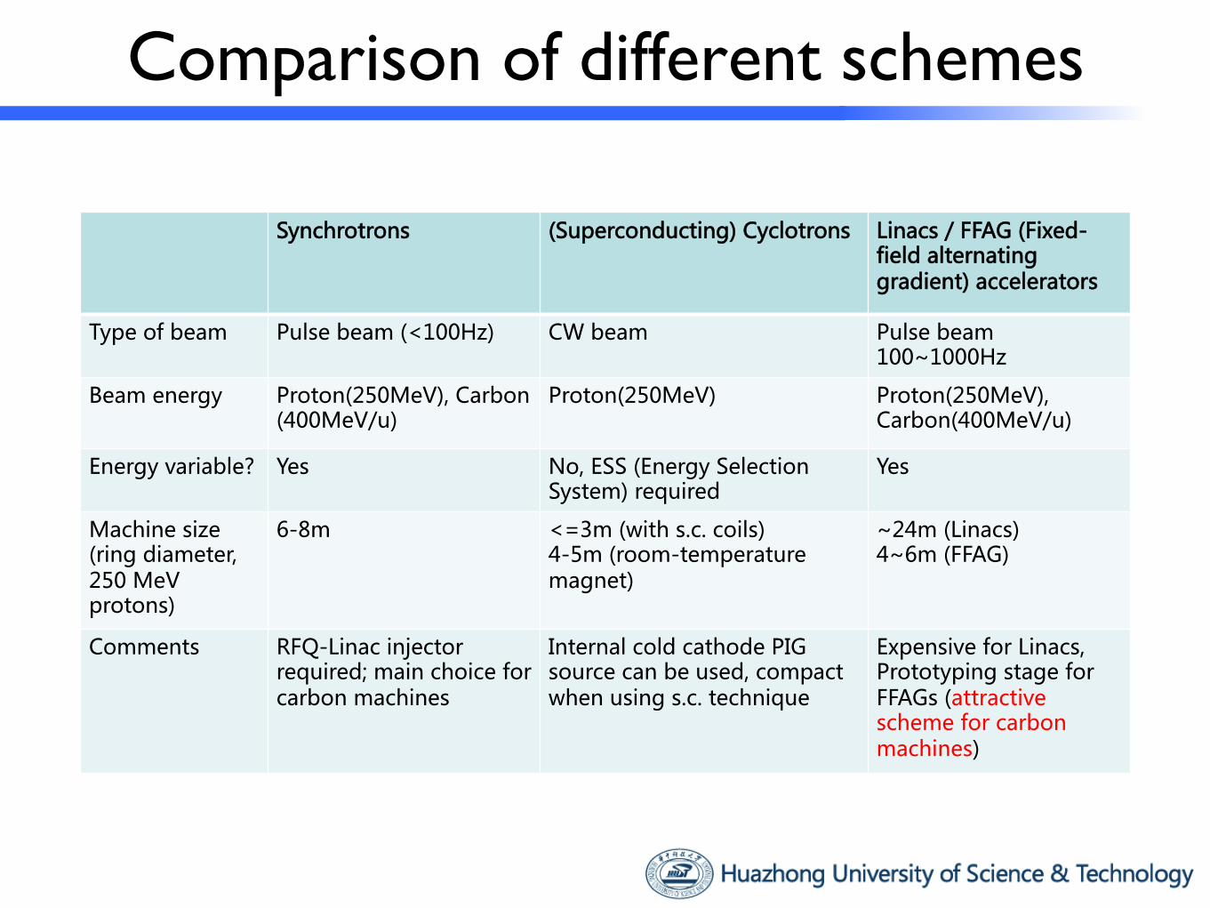
Comparison of different schemes

Synchrotrons (Superconducting) Cyclotrons Linacs / FFAG (Fixed-field alternating gradient) accelerators

Type of beam Pulse beam (<100Hz) CW beam Pulse beam 100~1000Hz

Beam energy Proton(250MeV), Carbon(400MeV/u)

Proton(250MeV) Proton(250MeV), Carbon(400MeV/u)

Energy variable? Yes No, ESS (Energy Selection System) required

Yes

Machine size (ring diameter, 250 MeV protons)

6-8m <=3m (with s.c. coils) 4-5m (room-temperature magnet)

~24m (Linacs) 4~6m (FFAG)

Comments RFQ-Linac injector required; main choice for carbon machines

Internal cold cathode PIG source can be used, compact when using s.c. technique

Expensive for Linacs, Prototyping stage for FFAGs (attractive scheme for carbon machines)

Two main schemes for proton machines

MSU/PSI/Accel scheme Superconducting isochronous cycltron: 3T @ ext., 3.2m diameter, internal cold cathode PIG; fixed RF (Coutesy of H. Rocken, CYC2010)

! IBA S2C2 (superconducting synchro-cyclotron): max. [email protected]., 2.5m diameter, internal cold cathode PIG; 1k Hz rotco RF (Coutesy of W. Kleeven, MO4PB02, CYC2013)

We chose

OUTLINE

p Motivation & & schemes comparison

p Design study

p Overall considerations

p Spiral magnet design

p Isochronous field trimming

p Precessional extraction

p Conclusions

General features of s.c. cyclotron

4 rf cavity& power feed in

YOKE

SC Coil

2 Deflectors

Ext. Magnet Channels

4 spiral

poles

PIG source& C.R.

1) Internal cold cathode PIG source, simplification of injection, for moderate intensity ~500nA

2) NbTi/Cu composite superconductor with liquid Helium cooling, maximum 3.2 T average field at extraction

2) Spiral shape magnet, for stable axial focusing in low flutter condition

4) Precessional extraction: by generating small first harmonic bump before Nu_r=1.0 resonance crossing, enlarge last turn separation.

Overall parameters

Spiral shape magnet

!"#$ %&'% %()*+, -./ %01#22#.-

-.3 '/ 451

()67)8+, '3 '( 9 ' :); '

''

!" #<%)22'=>?'0'<3)22'=@?'0'()AB22%'.')C:3*A6&'

' =)C)<6)C)%?D' 3'

Author's personal copyARTICLE IN PRESS

! For the side shimming points, they are designed to counter-balance neighboring shimming value with the displacementdLside, k " 1

4 #bk$1%bk&.

In computation models of the magnet, the pole edge is directlyconnected by the main and side shimming points in order to easethe modeling process. However, during the machining of the poleedge after field mapping, a cubic spline interpolation among theseshimming points is suggested to obtain a smooth pole shape.

3.3. Comparative results

The proposed matrix method is applied on the initial magnetmodel illustrated in Fig. 1. After performing the equilibrium orbitcalculation, the gyration frequency error and isochronous fielderror are acquired, as shown in Figs. 9 and 10. For a comparativestudy, the hard edge approximation is also used. Fig. 8 showsshimming vectors calculated independently by the original leastsquare fit, the improved solution with artificial adjustment, thehard edge approximation with the scaling factor 1.0 and 0.8. Theresult also shows the hard edge approximation has anundervaluation on the shimming value, as is mentioned inSection 3.1.

Fig. 9 exhibits the calculated isochronous field error andvarious shimming effects with above methods. It is obvious thatthe proposed matrix method gives a more precise compensationfor the isochronous field error. Due to the deficiency on describingnonlinear radial fringe field, there exists considerable discrepancyto the desired shimming effect when using the hard edgeapproximation. A fast convergence of the magnetic fieldisochronism can be achieved with the proposed matrix method.As seen in Fig. 10, after second iteration using the improvedmatrix method, the relative gyration frequency error is controlledwithin 0.02%, and the history phase slip is o783.

4. Considerations on beam dynamics and pole end shaping

Beyond the requirement of isochronism condition, the mag-netic field distribution of compact cyclotrons should providesufficient transversal focusing of the beam, as well as avoid

dangerous resonance crossing during beam acceleration, or atleast pass through quickly.

The horizontal tune nr and vertical betatron tune nz of beamdepend on multiple parameters of the magnet, which can beapproximately expressed by [3]

n2r " 1%k%3N2

#N2$1&#N2$4&F#1%tan2 x& #8&

n2z "$k%N2

N2$1F#1%2 tan2 x& #9&

where k" #r=B&#@B=@r& is the radial field index, F " #B2$B2&=B

2is

the flutter of the magnetic field, and x is the spiral angle.

Fig. 8. Comparative shimming vector for the initial magnet model calculated by:(1) least square fit; (2) improved solution with artificial adjustment; (3) hard edgemodel with scaling factor 1.0; and (4) hard edge model with scaling factor 0.8.

Fig. 9. Shimming effects using various shimming vectors.

Fig. 10. Top: gyration frequency error with two shimming methods andbottom: corresponding history phase slip.

B. Qin et al. / Nuclear Instruments and Methods in Physics Research A 620 (2010) 121–127 125

'< '% '< 3)

''

E'=F2?' GHIJ#K'#LMK+'=N+MC?'<)' O'%)' <O'/)' /O'3)' (O'()' 7O'7)' O3'O)' O(':)' O7'

'( *PE6%*PQ.)

''

Superconducting coil induced field possesses dominant part, and the field flutter contributed from pole hill and valley structure is much lower. (F<0.1)

For axial focusing, to compensate , spiral angle must be introduced

−k = −(γ2 − 1)

Flutter optimization and max. spiral angle

Table 1: Overall parameters

Extraction energy 250 MeVIon source Internal P.I.G. sourceBeam intensity ! 500nAEmmittance 5!mm ·mradInjection / extraction field 2.45 / 3.1 TSpiral angel (maximum) 66 degreesPole gap at hill 5 cmPole radius 84 cmTotal ampere turns 1.2MA · TRF frequency 74MHz (harmonic mode=2)Energy gain per turn ! 400keVExtraction scheme Precessional extraction

MAGNET DESIGN AND TUNE

OPTIMIZATION

Optimization of the flutter and the spiral angle

The magnet model built by TOSCA [6] is shown in Fig. 1.Compared to room temperature magnet, the superconduct-ing coil induced field possesses dominant part, and the fieldflutter contributed by pole hill and valley structure is muchlower. Since "2

z ! "k +F · (1 + 2 tan2 # ), and the field indexk = $2

" 1 is pre-determined to maintain isochronous con-dition, a spiral angle must be introduced to compensate theinstability of "k .

For a given extraction energy $ext, the maximum spiralangle has a strong relation to the flutter at the extraction area.To reduce this spiral angle for achieving higher rf voltage,the flutter is optimized by choosing a suitable ratio of hill /valley gaps. Also, the coil field need be controlled to avoiddecreasing the flutter. Fig. 2 shows the optimization of theflutter and the final flutter is beyond 0.05 for main accelera-tion area.

Figure 1: Magnet model

Normally "2r ! 1 + k = $2 is smoothly changed by beam

energy, but, to maintain a stable vertical tune, the spiral an-gle need be adjusted along the radius. A python script was

0 10 20 30 40 50 60 70 80

Radius / cm

0.00

0.01

0.02

0.03

0.04

0.05

0.06

0.07

0.08

Flu

tter

After optimization

Before optimization

Figure 2: Optimization of the flutter

developed to modify the spiral angel in the tosca model, ac-cording to the calculated tune variation. Finally, a well con-trolled tune shift was obtained, as shown in Fig. 3.

0.7 0.8 0.9 1.0 1.1 1.2 1.3 1.4 1.50.0

0.1

0.2

0.3

0.4

0.5

0.6

0.7

0.8

Figure 3: Tune diagram during acceleration, only third res-onances drawn

Isochronous field shimming with trim rods

For cyclotrons with room-temperature magnet, theisochronous field can be achieved by pole shaping precisely[7]. However, as addressed, the field component producedby the superconducting coils and iron pole saturation makespole shaping not so e!cient.

Two steps are used for field isochronism: 1) For meet-ing initial isochronous field condition, the hill pole width isincreased from the central region to the pole end, with an it-erative process by evaluating the field generated by TOSCAmodel. As shown in Fig. 4, the isochronous field error canbe limited within 150 Gs. 2) Fine shimming by using trimrods. As shown in Fig. 5, 29 trim rods are located at thecenter line of the spiral pole, and the independent field shim-ming e"ect when removing these rods are shown in Fig. 6.For the trim rods with same surface area, the shimming ef-fect will decrease along the pole radius due to the increasing

is pre-determined by field isochronism condition à


Extraction energy 250 MeVIon source Internal P.I.G. sourceBeam intensity ! 500nAEmmittance 5!mm ·mradInjection / extraction field 2.45 / 3.1 TSpiral angel (maximum) 66 degreesPole gap at hill 5 cmPole radius 84 cmTotal ampere turns 1.2MA · TRF frequency 74MHz (harmonic mode=2)Energy gain per turn ! 400keVExtraction scheme Precessional extraction

MAGNET DESIGN AND TUNE

OPTIMIZATION

Optimization of the flutter and the spiral angle

The magnet model built by TOSCA [6] is shown in Fig. 1.Compared to room temperature magnet, the superconduct-ing coil induced field possesses dominant part, and the fieldflutter contributed by pole hill and valley structure is muchlower. Since "2

z ! "k +F · (1 + 2 tan2 # ), and the field indexk = $2

" 1 is pre-determined to maintain isochronous con-dition, a spiral angle must be introduced to compensate theinstability of "k .

For a given extraction energy $ext, the maximum spiralangle has a strong relation to the flutter at the extraction area.To reduce this spiral angle for achieving higher rf voltage,the flutter is optimized by choosing a suitable ratio of hill /valley gaps. Also, the coil field need be controlled to avoiddecreasing the flutter. Fig. 2 shows the optimization of theflutter and the final flutter is beyond 0.05 for main accelera-tion area.


Normally "2r ! 1 + k = $2 is smoothly changed by beam

energy, but, to maintain a stable vertical tune, the spiral an-gle need be adjusted along the radius. A python script was

0 10 20 30 40 50 60 70 80

Radius / cm

0.00

0.01

0.02

0.03

0.04

0.05

0.06

0.07

0.08

Flu

tter

After optimization

Before optimization


developed to modify the spiral angel in the tosca model, ac-cording to the calculated tune variation. Finally, a well con-trolled tune shift was obtained, as shown in Fig. 3.

0.7 0.8 0.9 1.0 1.1 1.2 1.3 1.4 1.50.0

0.1

0.2

0.3

0.4

0.5

0.6

0.7

0.8

Figure 3: Tune diagram during acceleration, only third res-onances drawn

Isochronous field shimming with trim rods

For cyclotrons with room-temperature magnet, theisochronous field can be achieved by pole shaping precisely[7]. However, as addressed, the field component producedby the superconducting coils and iron pole saturation makespole shaping not so e!cient.

Two steps are used for field isochronism: 1) For meet-ing initial isochronous field condition, the hill pole width isincreased from the central region to the pole end, with an it-erative process by evaluating the field generated by TOSCAmodel. As shown in Fig. 4, the isochronous field error canbe limited within 150 Gs. 2) Fine shimming by using trimrods. As shown in Fig. 5, 29 trim rods are located at thecenter line of the spiral pole, and the independent field shim-ming e"ect when removing these rods are shown in Fig. 6.For the trim rods with same surface area, the shimming ef-fect will decrease along the pole radius due to the increasing

l  Installation of RF cavity and higher RF voltage need the spiral angle as small as possible

l  Spiral angle is modulated along the radius, reach maximum at extraction

Enhanced field flutter by optimizing the magnet structure

kext

kext = γ2ext − 1 ≈ 0.6

ζext ≈ 65◦

Stabilization of axial motion and tune diagram

• Precessional beam extraction: The last turn separation dueto acceleration is less than 1mm, which can be increasedto 5mm by introducing a first harmonic field bump nearthe resonance crossing line !r = 1.0, with the precessionalextraction method.


Extraction energy 250 MeVIon source Internal cold cathode PIG sourceBeam intensity ! 500nAEmmittance 5"mm ·mradInjection / extraction field 2.45 / 3.1 TSpiral angel (maximum) 66 degreesPole gap at hill 5 cmPole radius 84 cmTotal ampere turns 1.2MA · TRF frequency 74MHz (harmonic mode=2)Energy gain per turn ! 400keVExtraction scheme Precessional extraction

3. Magnet design and tune optimization

3.1. Optimization of the flutter and the spiral angleThe magnet model built by TOSCA[6] is shown in Fig. 1.

Compared to room temperature magnet, the superconductingcoil induced field possesses dominant part, and the field flut-ter contributed by pole hill and valley structure is much lower.Since !2z ! "k + F · (1+ 2 tan2 #), and the field index k = $2 " 1is pre-determined to maintain isochronous condition, a spiralangle must be introduced to compensate the instability of "k.For a given extraction energy $ext, the maximum spiral angle

has a strong relation to the flutter at the extraction area. To re-duce this spiral angle for achieving higher rf voltage, the flutteris optimized by choosing a suitable ratio of hill / valley gaps.Also, the coil field need be controlled to avoid decreasing theflutter. Fig. 2 shows the optimization of the flutter and the finalflutter is beyond 0.05 for main acceleration area.Normally !2r ! 1 + k = $2 is smoothly changed by beam

energy, but, to maintain a stable vertical tune, the spiral angleneed be adjusted along the radius. A python script was devel-oped to modify the spiral angel in the tosca model, accordingto the calculated tune variation. Finally, a well controlled tuneshift was obtained, as shown in Fig. 3.

3.2. Isochronous field shimming with trim rodsFor cyclotrons with room-temperature magnet, the

isochronous field can be achieved by pole shaping precisely[7].However, as addressed, the field component produced by thesuperconducting coils and iron pole saturation makes poleshaping not so e!cient.Two steps are used for field isochronism: 1) For meeting ini-

tial isochronous field condition, the hill pole width is increasedfrom the central region to the pole end, with an iterative process


0 10 20 30 40 50 60 70 80

Radius / cm

0.00

0.01

0.02

0.03

0.04

0.05

0.06

0.07

0.08

Flu

tter

After optimization

Before optimization


0.7 0.8 0.9 1.0 1.1 1.2 1.3 1.4 1.50.0

0.1

0.2

0.3

0.4

0.5

0.6

0.7

0.8

Figure 3: Tune diagram during acceleration, only third resonances drawn

by evaluating the field generated by TOSCA model. As shownin Fig. 4, the isochronous field error can be limited within 150Gs. 2) Fine shimming by using trim rods. As shown in Fig. 5,29 trim rods are located at the center line of the spiral pole,

2

• Precessional beam extraction: The last turn separation dueto acceleration is less than 1mm, which can be increasedto 5mm by introducing a first harmonic field bump nearthe resonance crossing line !r = 1.0, with the precessionalextraction method.


Extraction energy 250 MeVIon source Internal cold cathode PIG sourceBeam intensity ! 500nAEmmittance 5"mm ·mradInjection / extraction field 2.45 / 3.1 TSpiral angel (maximum) 66 degreesPole gap at hill 5 cmPole radius 84 cmTotal ampere turns 1.2MA · TRF frequency 74MHz (harmonic mode=2)Energy gain per turn ! 400keVExtraction scheme Precessional extraction

3. Magnet design and tune optimization

3.1. Optimization of the flutter and the spiral angleThe magnet model built by TOSCA[6] is shown in Fig. 1.

Compared to room temperature magnet, the superconductingcoil induced field possesses dominant part, and the field flut-ter contributed by pole hill and valley structure is much lower.Since !2z ! "k + F · (1+ 2 tan2 #), and the field index k = $2 " 1is pre-determined to maintain isochronous condition, a spiralangle must be introduced to compensate the instability of "k.For a given extraction energy $ext, the maximum spiral angle

has a strong relation to the flutter at the extraction area. To re-duce this spiral angle for achieving higher rf voltage, the flutteris optimized by choosing a suitable ratio of hill / valley gaps.Also, the coil field need be controlled to avoid decreasing theflutter. Fig. 2 shows the optimization of the flutter and the finalflutter is beyond 0.05 for main acceleration area.Normally !2r ! 1 + k = $2 is smoothly changed by beam

energy, but, to maintain a stable vertical tune, the spiral angleneed be adjusted along the radius. A python script was devel-oped to modify the spiral angel in the tosca model, accordingto the calculated tune variation. Finally, a well controlled tuneshift was obtained, as shown in Fig. 3.

3.2. Isochronous field shimming with trim rodsFor cyclotrons with room-temperature magnet, the

isochronous field can be achieved by pole shaping precisely[7].However, as addressed, the field component produced by thesuperconducting coils and iron pole saturation makes poleshaping not so e!cient.Two steps are used for field isochronism: 1) For meeting ini-

tial isochronous field condition, the hill pole width is increasedfrom the central region to the pole end, with an iterative process


0 10 20 30 40 50 60 70 80

Radius / cm

0.00

0.01

0.02

0.03

0.04

0.05

0.06

0.07

0.08

Flu

tter

After optimization

Before optimization


0.7 0.8 0.9 1.0 1.1 1.2 1.3 1.4 1.50.0

0.1

0.2

0.3

0.4

0.5

0.6

0.7

0.8

Figure 3: Tune diagram during acceleration, only third resonances drawn

by evaluating the field generated by TOSCA model. As shownin Fig. 4, the isochronous field error can be limited within 150Gs. 2) Fine shimming by using trim rods. As shown in Fig. 5,29 trim rods are located at the center line of the spiral pole,

2

l  varies smoothly as

l  controlled by local spiral angle à modified according to the tune values

iteratively, automatically by a Python script

l  avoided; l  Walkinshaw resonance

avoided in main acceleration region

νr νr ≈ γ

νz

νr − νz = 1νr − 2νz = 0

Isochronous field shaping / trimming

and the independent field shimming e!ect when removing theserods are shown in Fig. 6. For the trim rods with same surfacearea, the shimming e!ect will decrease along the pole radiusdue to the increasing circumference. To compensate this, tworod radius are used, with inner part 1cm and outer part 2cm.For consideration on technical issues, two vertical positions ofthe trim rods (2cm / 1cm to the pole surface) are used, and acode was written to get the combination the rods positions byadjusting the result from least square fit.By combining these two methods, 0.05% local field error and±15! total phase slip can be achieved.

0 10 20 30 40 50 60 70 80

Radius / cm

1.5

2.0

2.5

3.0

3.5

Aver

age

fiel

d/T

Average field in tosca model

Isochronous field

Figure 4: Average field with initial isochronous shaping

Figure 5: Trim rods located at the center of spiral pole, for fine shimming ofthe isochronous field

0 10 20 30 40 50 60 70 80 90−250

−200

−150

−100

−50

0

50

Radius / cm

dB /

Gs

Figure 6: Independent field shimming e!ect with 2cm depth

4. Precessional extraction

For high magnetic field around 3T at the extraction, the turnseparation due to energy gain is lower than 1mm, which bringssignificant beam loss when ”cutting” by the septum in the elec-tronic deflector. Meantime the energy spread will be enlarged.A mature method, single turn precessional extraction [8] can beemployed to increase the turn separation.By generating a first harmonic field bump b1(r, !) = b1(r) ·

cos(! " !0), before the "r = 1 resonance crossing, at a givenazimuthal angle !0, a coherent oscillation is created and the re-sulting radial displacement is:

"Rpre = #R · "$(b1/B(R)) (1)

The bump field can be generate either by harmonic coils ortrim rod. Fig. 7 shows the simulation on tracing the beam en-velope using b1 = 6Gs, !0 = 30!, the e!ective turns duringcoherent oscillation "$ = 9. The final turn separation was en-larged to "R = 5.3mm including the acceleration component,which is coincident with the theoretical value "Rpre = 4.5mm.In simulation, the beam is pre-centered by using the accelerat-ing equilibrium orbit(A.E.O.).

Figure 7: Precession extraction, using a 6Gs harmonic bump

5. Conclusion and discussion

Preliminary design considerations on an isochronous super-conducting cyclotron aiming at proton therapy are described,mainly focusing on overall design, magnet, and extractionscheme. Some other system, important as well, such as therf cavity, the superconducting coil / Dewar, the central regionand the extraction structure are under design progress and notpresented.Considering the target patients for asian people, 235MeV ex-

traction energy is also a choice.[1] U. Amaldi et al., Nucl. Instr. and Meth. A 620 (2010) 563-577.[2] FANG Shouxian, TANG Jingyu, GUAN Xialing et al., Conceptual design

for Advance Proton Therapy Facility (APTF), 8th National Symposium onMedical Accelerators.

[3] T.J. Zhang, private communication.[4] Jong-Won Kim, Nucl. Instr. and Meth. A 582 (2007) 366-373[5] D. Rifuggiato et al., Variety of beam production at the INFN LNS super-

conducting cyclotron, Proceedings of CYCLOTRONS 2013, MOPPT011.[6] Opera-3D User Guide,Vector Fields Limited, England.[7] B. Qin et al., Nucl. Instr. and Meth. A 691(2012) 129-134[8] M. M. Gordon, Single turn extraction, IEEE Trans. Nucl. Sci., 13 (4), 48-

57

3

Magnet poles saturated in high magnetic field, pole shimming is not so efficient Two steps: 1)  For meeting initial isochronous

field condition, the hill pole width is increased from the central region to the pole end, Field error can be limited within 150 Gs. Average field with initial isochronous

shaping; iterative process by evaluating tosca models.


0 10 20 30 40 50 60 70 80

Radius / cm

1.5

2.0

2.5

3.0

3.5

Aver

age

fiel

d/T


Isochronous field



0 10 20 30 40 50 60 70 80 90−250

−200

−150

−100

−50

0

50

Radius / cm

dB /

Gs





"Rpre = #R · "$(b1/B(R)) (1)









57

3


0 10 20 30 40 50 60 70 80

Radius / cm

1.5

2.0

2.5

3.0

3.5

Aver

age

fiel

d/T


Isochronous field



0 10 20 30 40 50 60 70 80 90−250

−200

−150

−100

−50

0

50

Radius / cm

dB /

Gs





"Rpre = #R · "$(b1/B(R)) (1)









57

3

Limitations: 1)  Nonlinear relations between rods

depth & trimming effect; 2)  Technical difficulties for arbitrary

depth adjustment 3)  Two positions are adopted for each

rods, +/-15 degrees total phase slip achieved

from measurement data, one can calculate gyration frequencyfp(r) as a function of the pole radius r (transformed from particleenergy), using equilibrium orbit codes which is based on thenumerical integration on field maps, like PTP [12]. Then theisochronous field error DB!r" can be evaluated using the followingequation:

DB!r" # B!r"$Biso!r" % B!r" &g2!r" & Df !r"

1'g2!r" &Df !r" !1"

where Biso!r" is the estimated isochronous field at radius r, B(r) isthe calculated or measured azimuthally average field at radius r,g!r" % 1'Ek!r"=E0. Df !r" is the gyration frequency error defined byDf !r" # !f p!r"$f 0"=f 0, with f0 being the designed ion orbitalfrequency.

In order to obtain a precise estimation on the shimming valuefrom DB!r" which takes into account the radial fringe effect of thecutting patches, multiple linear regression can be employed withtwo assumptions: (1) the magnetic field change due to a cuttingpatch is proportional to the patch area and (2) the accumulatedmagnetic field change is equal to the superposition of the effectsdue to independent cutting patches along the radius. These havebeen validated by analytical formulas and numerical simulation[10], with the prerequisite that the cutting thickness is smallenough compared to the pole circumference.

First we define the magnetic field change vector y% (y1,y2, . . . ,yn)

T , in which yk % Bi!rk"$Bi$1!rk" corresponds to the field changeat radius rk from two adjacent iterations i$1 and i. y can becalculated by the following equation:

y%X & b !2"

where b% (b1,b2, . . . ,bm)T denotes the shimming vector with bj

corresponding to the normalized cutting thickness at radius rj. Xis a n*m correlation regressor matrix which is pre-calculatedfrom m set magnet models. For each model, small change insector shape is applied using a unit shimming vector bunit,j %(0, . . . ,bj % 1,0)T !j% 1, . . . ,m", and field change yj is extracted bycomparing the modified model with the original model. From Eq.(2), one obtains

Xj % (X1j,X2j, . . . ,Xnj)T % (yj1,yj2, . . . ,y

jn)

T : !3"

The same procedure is performed on j% 1, . . . ,m, then we havethe full correlation matrix X. Although the data is retrieved fromsimulation models with TOSCA code, it can be applied to the realisticpole shaping because the discrepancy between the TOSCA calcula-tion and the measured field is small, especially for prediction of thefield change. This will be demonstrated by our experimental data.For a isochronous field error yiso, the least square solution of Eq. (2)which minimizes the residuals e% JX & b$yJ is

b % !XT & X"$1 & XT & yiso: !4"

2.2. Improvements of the fundamental matrix method

The solution given by the least square fit provides a goodestimation of the magnet pole shimming. However, some factorsrelated to the correlation matrix need to be considered to avoidoscillation of b, and the final shimming effect should be evaluatedwith a more precise way in order to assure the safety of theshimming procedures.

2.2.1. Radial space for calculation of the correlation matrix andminor adjustment on the shimming vector

Oscillations of the least square fit solution will cause un-smooth pole edge, and more important, the negative elements arenot acceptable during practical shimming procedures. The study

shows that the radial space Dr has a significant influence on theseoscillations. By numerical comparison, we chose Dr% 20 mm forgood balance between the smooth in b and enough accuracy ofthe estimation.

The basic requirement for the shimming processes is thatbZ0 should be fulfilled when yisoZ0. Even with a good selectionof Dr, this condition is not always true for the least square fitsolution, then some adjustment on the shimming vector shouldbe performed. For example, if blo0, it will be reset to zero, andthe value of bl$1 and b l'1 is decreased to compensate theaccumulated shimming effect. By replacing the original b withthis improved vector bimp, the final predicted shimming effectypred can be calculated using ypred %X & bimp , again by Eq. (2).

2.2.2. Improvements on the prediction precision of the shimmingeffect and reduction in the computation time

For estimation of b by Eq. (4), Dr% 20 mm was selected. Asshown in Fig. 1, 11 models with a 20 mm*2 mm triangle areacutting corresponding to central cutting radii from 7 cm to 27 cmwith Dr% 20 mm were calculated and compared to the originalone, and the correlation matrix can be derived.

However, in order to have more precise prediction on theshimming effect, smaller step size for the correlation matrix X ispreferred. The blue dotted line in Fig. 2 shows the raw shimmingeffect retrieved from 11 TOSCA models, with Gaussian-like dis-tribution and decreasing peak field due to the smaller ratiocompared to the circumference along the radii. By performingthe spline interpolation on the raw data, we get 27 data setscorresponding to the shimming effect from r% 6 cm to r% 32 cmwith Dr% 10 mm, and a fine prediction correlation matrix Xpred

with dimension !n* 27" can be calculated. As discussed in theexperimental results, the shimming effect using Xpred has a verygood match to the field mapping data, which guarantees theshimming procedures within the control.

Since this matrix method heavily relies on the three-dimen-sional FEM field computation, techniques to reduce computationtime and manual operation are studied. Scripts written by Pythonare employed to facilitate automated modeling, calculation andfield acquisition based on the original magnet model, and inter-polation helps to reduce the number of calculation models. Aswell as an interface was built with functions including

Fig. 1. Pole cutting scheme for calculating field change compared to the originalmodel.

B. Qin et al. / Nuclear Instruments and Methods in Physics Research A 691 (2012) 129–134130

from measurement data, one can calculate gyration frequencyfp(r) as a function of the pole radius r (transformed from particleenergy), using equilibrium orbit codes which is based on thenumerical integration on field maps, like PTP [12]. Then theisochronous field error DB!r" can be evaluated using the followingequation:

DB!r" # B!r"$Biso!r" % B!r" &g2!r" & Df !r"

1'g2!r" &Df !r" !1"

where Biso!r" is the estimated isochronous field at radius r, B(r) isthe calculated or measured azimuthally average field at radius r,g!r" % 1'Ek!r"=E0. Df !r" is the gyration frequency error defined byDf !r" # !f p!r"$f 0"=f 0, with f0 being the designed ion orbitalfrequency.

In order to obtain a precise estimation on the shimming valuefrom DB!r" which takes into account the radial fringe effect of thecutting patches, multiple linear regression can be employed withtwo assumptions: (1) the magnetic field change due to a cuttingpatch is proportional to the patch area and (2) the accumulatedmagnetic field change is equal to the superposition of the effectsdue to independent cutting patches along the radius. These havebeen validated by analytical formulas and numerical simulation[10], with the prerequisite that the cutting thickness is smallenough compared to the pole circumference.

First we define the magnetic field change vector y% (y1,y2, . . . ,yn)

T , in which yk % Bi!rk"$Bi$1!rk" corresponds to the field changeat radius rk from two adjacent iterations i$1 and i. y can becalculated by the following equation:

y%X & b !2"

where b% (b1,b2, . . . ,bm)T denotes the shimming vector with bj

corresponding to the normalized cutting thickness at radius rj. Xis a n*m correlation regressor matrix which is pre-calculatedfrom m set magnet models. For each model, small change insector shape is applied using a unit shimming vector bunit,j %(0, . . . ,bj % 1,0)T !j% 1, . . . ,m", and field change yj is extracted bycomparing the modified model with the original model. From Eq.(2), one obtains

Xj % (X1j,X2j, . . . ,Xnj)T % (yj1,yj2, . . . ,y

jn)

T : !3"

The same procedure is performed on j% 1, . . . ,m, then we havethe full correlation matrix X. Although the data is retrieved fromsimulation models with TOSCA code, it can be applied to the realisticpole shaping because the discrepancy between the TOSCA calcula-tion and the measured field is small, especially for prediction of thefield change. This will be demonstrated by our experimental data.For a isochronous field error yiso, the least square solution of Eq. (2)which minimizes the residuals e% JX & b$yJ is

b % !XT & X"$1 & XT & yiso: !4"

2.2. Improvements of the fundamental matrix method

The solution given by the least square fit provides a goodestimation of the magnet pole shimming. However, some factorsrelated to the correlation matrix need to be considered to avoidoscillation of b, and the final shimming effect should be evaluatedwith a more precise way in order to assure the safety of theshimming procedures.

2.2.1. Radial space for calculation of the correlation matrix andminor adjustment on the shimming vector

Oscillations of the least square fit solution will cause un-smooth pole edge, and more important, the negative elements arenot acceptable during practical shimming procedures. The study

shows that the radial space Dr has a significant influence on theseoscillations. By numerical comparison, we chose Dr% 20 mm forgood balance between the smooth in b and enough accuracy ofthe estimation.

The basic requirement for the shimming processes is thatbZ0 should be fulfilled when yisoZ0. Even with a good selectionof Dr, this condition is not always true for the least square fitsolution, then some adjustment on the shimming vector shouldbe performed. For example, if blo0, it will be reset to zero, andthe value of bl$1 and b l'1 is decreased to compensate theaccumulated shimming effect. By replacing the original b withthis improved vector bimp, the final predicted shimming effectypred can be calculated using ypred %X & bimp , again by Eq. (2).

2.2.2. Improvements on the prediction precision of the shimmingeffect and reduction in the computation time

For estimation of b by Eq. (4), Dr% 20 mm was selected. Asshown in Fig. 1, 11 models with a 20 mm*2 mm triangle areacutting corresponding to central cutting radii from 7 cm to 27 cmwith Dr% 20 mm were calculated and compared to the originalone, and the correlation matrix can be derived.

However, in order to have more precise prediction on theshimming effect, smaller step size for the correlation matrix X ispreferred. The blue dotted line in Fig. 2 shows the raw shimmingeffect retrieved from 11 TOSCA models, with Gaussian-like dis-tribution and decreasing peak field due to the smaller ratiocompared to the circumference along the radii. By performingthe spline interpolation on the raw data, we get 27 data setscorresponding to the shimming effect from r% 6 cm to r% 32 cmwith Dr% 10 mm, and a fine prediction correlation matrix Xpred

with dimension !n* 27" can be calculated. As discussed in theexperimental results, the shimming effect using Xpred has a verygood match to the field mapping data, which guarantees theshimming procedures within the control.

Since this matrix method heavily relies on the three-dimen-sional FEM field computation, techniques to reduce computationtime and manual operation are studied. Scripts written by Pythonare employed to facilitate automated modeling, calculation andfield acquisition based on the original magnet model, and inter-polation helps to reduce the number of calculation models. Aswell as an interface was built with functions including

Fig. 1. Pole cutting scheme for calculating field change compared to the originalmodel.

B. Qin et al. / Nuclear Instruments and Methods in Physics Research A 691 (2012) 129–134130

Isochronous field shaping / trimming Two steps: 2)  Fine shimming by using trim rods. Combination of trim rods position based on the least square fitting from the correlation matrix:

Precessional extraction – beam centering by A.E.O

Gordan’s method1: Quasi-fixed center, (x,px) to be the same after one turn acceleration

! !

1M. M. Gordon, Single turn extraction, IEEE Trans. Nucl. Sci., 13 (4), 48-57

210-230MeV, 0.6MeV/turn, (L)not centered; (R)centered

x(E, θ) = r(E, θ)− re(E, θ)px(E, θ) = pr(E, θ)− pre(E, θ)

(re, pre) refers to coordinates in static equilibrium orbit

For high efficient resonant extraction, beams need be pre-centered using

accelerating E.O. àTo remove coherent oscillation effects

àTurns are evenly spaced, before using the field bump

Precessional extraction and the independent field shimming e!ect when removing theserods are shown in Fig. 6. For the trim rods with same surfacearea, the shimming e!ect will decrease along the pole radiusdue to the increasing circumference. To compensate this, tworod radius are used, with inner part 1cm and outer part 2cm.For consideration on technical issues, two vertical positions ofthe trim rods (2cm / 1cm to the pole surface) are used, and acode was written to get the combination the rods positions byadjusting the result from least square fit.By combining these two methods, 0.05% local field error and±15! total phase slip can be achieved.

0 10 20 30 40 50 60 70 80

Radius / cm

1.5

2.0

2.5

3.0

3.5

Aver

age

fiel

d/T


Isochronous field



0 10 20 30 40 50 60 70 80 90−250

−200

−150

−100

−50

0

50

Radius / cm

dB /

Gs





"Rpre = #R · "$(b1/B(R)) (1)









57

3

b1=10Gs, =30 deg., dR~8mm

b1=6Gs, =30 deg., dR~5mm (coincident with theoretical 4.3mm, eff. Turns = 9)

effective turns during coherent oscillation

By generating a first harmonic field Before resonance crossing , at , a coherent oscillation is created and

b1(r, θ) = b1(r) · cos(θ − θ0)

νr = 1 θ0

∆τ = ((∆νr/∆E) · Egain))−1/2

Ø  The radial and azimuthal position of the field bump is very sensitive;

Ø  b1 ban be generated by harmonic coil or trim rod

θ0

θ0

Conclusions

•  A 250 MeV/ 500nA isochronous superconducting cyclotron for proton therapy was proposed by HUST, and collaborated with CAS-IPP;

•  Preliminary design considerations including overall scheme, main magnet, resonant extraction and rf etc. are introduced;

•  The central region, the extraction structure (septum, high voltage feed in, deflectors, magnetic channel) are under design progress;

•  Considering the target patients for Asia area, 235MeV extraction energy is also a choice.

Thanks for attention!

design study of a 250mev superconducting...

Documents