1

Design of Resilient Supply Chains with Risk of Facility Disruptions P. Garcia-Herreros1; J.M. Wassick2 & I.E. Grossmann1 1Department of Chemical Engineering, Carnegie Mellon University, Pittsburgh, PA 15213 2The Dow Chemical Company. Midland, MI, 48674, USA Abstract The design of resilient supply chains under the risk of disruptions at candidate locations for distribution centers (DCs) is formulated as a two-stage stochastic program. The problem involves selecting DC locations, determining storage capacities for multiple commodities, and establishing the distribution strategy in scenarios that describe disruptions at potential DCs. The objective is to minimize the sum of investment cost and expected distribution cost during a finite time-horizon. The rapid growth in the number of scenarios requires the development of an effective method to solve large-scale problems. The method includes a strengthened multi-cut Benders decomposition algorithm and the derivation of deterministic bounds based on the optimal solution over reduced sets of scenarios. Resilient designs for a large-scale example and an industrial supply chain are found with the proposed method. The results demonstrate the importance of including DC capacity in the design problem and anticipating the distribution strategy in adverse scenarios.

1. Introduction Supply chain resilience has recently become one of the main concerns for major companies. The increasing complexity and interdependency of logistic networks have contributed to enhance the interest on this topic. A recent report presented by the World Economic Forum indicates that supply chain disruptions reduce the share price of impacted companies by 7% on average (Bathia et al., 2013). One emblematic case of supply chain resilience happened in 2000 when a fire at the Philips microchip plant in Albuquerque (NM) cut off the supply of a key component for cellphone manufacturers Nokia and Ericsson. Nokia’s production lines were able to adapt quickly by using alternative suppliers and accepting similar components. In contrast, the supply disruption had a significant impact in Ericsson’s production causing an estimate loss in revenue of $400 million (Latour, 2001). Similarly, the disruptions caused by hurricane Katrina in 2005 (Nwazota, 2005) and the earthquake that hit Japan in 2011 (Krausmann & Cruz, 203) exposed the vulnerabilities of centralized supply chain strategies in the process industry. The importance of building resilient supply chain networks and quantifying the effect of unexpected events in their operation has been recognized by several studies (Helferich & Cook, 2002; Rice & Caniato, 2003; Chopra & Sodhi, 2004; Craighead & Blackhurst, 2007). They advocate for the inclusion of risk reduction strategies into the supply chains design. However, disruptions are often neglected from the supply chain analysis because of their unpredictable and infrequent nature. Disruptions comprise a wide variety of events that prevent supply chains from their normal operation. Regardless of their nature, disruptions produce undesirable effects: they shut down parts of the network and force rearrangements of the logistic strategy that can be very expensive. Furthermore, the current paradigm of lean inventory management leads to reduced supply chain flexibility and increased vulnerability to disruptions. In order to implement reliable networks that consistently deliver high performance, the value of supply chain resilience must be considered during their design (Tomlin, 2006; Schütz & Tomasgard, 2011). Traditionally, the mathematical formulation of the supply chain design has been based on the facility location problem (FLP) (Weber & Friedrich, 1929; Geoffrion & Graves, 1974). The FLP implies

2

selecting among a set of candidate locations the facilities that offer the best balance between investment and transportation cost to a given set of demand points. The supply chain design problem has a broader scope. It also includes the role of suppliers, inventory management, and timing of deliveries. This paper addresses the design of multi-commodity supply chains subject to disruptions risk at the distribution centers (DCs). The problem involves selecting DC locations, establishing their storage capacity, and determining a distribution strategy that anticipates potential disruptions at DCs. The goal is to obtain the supply chain with minimum cost from a risk neutral perspective. The cost of the supply chain is calculated as the sum of investment cost and expected distribution cost over a finite time-horizon. Unlike previous work, this research considers DC storage capacities as a design variable that impacts investment cost and inventory availability. This approach follows from the intuitive notion that supply chain resilience requires backup capacity. The goal is to demonstrate that significant increases in network reliability can be obtained with reasonable increases in investment cost through appropriate capacity selection and allocation of inventories. In order to establish the optimal amount of inventories at DCs, demand assignments under the possible realizations of disruptions must be anticipated. Therefore, the problem is formulated in the context of two-stage stochastic programming with full recourse (Birge & Louveaux, 2011). First-stage decisions comprise the supply chain design: DC selection and their capacities. The second-stage decisions model the distribution strategy in the scenarios given by the potential combinations of active and disrupted locations. The solution of large-scale problems requires the development of specialized algorithms given the exponential growth in the number of scenarios with the increase in candidate DCs. Different versions of Benders decomposition (Benders, 1962) that exploit problem structure are presented. The remaining of the paper is organized as follows. Section 2 reviews the relevant contributions to the design of resilient supply chains. Section 3 formalizes the problem statement. Section 4 describes the mathematical formulation of the problem. Section 5 illustrates the model with a small example. In section 6, the solution method for the design of large-scale resilient supply chains is developed. Section 7 discusses some issues related to the implementation. Section 8 demonstrates the implementation of the solution strategy in a large-scale example. Section 9 formulates the design problem for a resilient supply chain from the process industry and presents its results. Finally, conclusions are drawn in section 10.

2. Literature Review Facility location problems have received significant attention since the theory of the location of industries was introduced by Weber & Friedrich (1929). In the context of supply chains, Geoffrion & Graves (1974) proposed a Mixed-Integer Linear Programming (MILP) formulation that contains the essence of subsequent developments. Several authors have continued developing different versions of this formulation. Owen & Daskin (1998), Meixell & Gargeya (2005), and Shen (2007) offer comprehensive reviews on facility location and supply chain design. Shah (2005) reviews the main developments in supply chains design and planning for the process industry. A review of the FLP under uncertainty is presented by Snyder (2006). Additionally, the design of robust supply chains under uncertainty is reviewed by Klibi et al (2010). Most recent efforts have included inventory management under demand uncertainty into the supply chain design (Tsiakis et al., 2001; Daskin et al., 2002; Coullard & Daskin, 2003; You & Grossmann, 2008). These formulations exploit the variance reduction that is achieved when uncertain demands are centralized at few DCs, according to the risk pooling effect demonstrated by Eppen (1979). The benefits of centralization contrast with the risk diversification effect that becomes apparent when supply

3

availability is considered uncertain. Snyder & Shen (2006) demonstrate that centralized supply chains are more vulnerable to the effect of supply uncertainty. The effect of unreliable supply in inventory management has been studied by several authors (Tomlin, 2006; Parlar & Berkin, 1991; Berk & Arreola-Risa, 1994; Qi et al., 2009). Qi et al (2010) integrated inventory decisions into the supply chain design with unreliable supply. The main approach to address uncertainty in supply availability is to allocate safety stock at DCs to mitigate the risk of running out of stock. The FLP under the risk of disruptions was originally studied by Snyder & Daskin (2005). They formulate a problem in which all candidate DCs have unlimited capacities and the same disruption probability. The model avoids the generation of scenarios by establishing customer assignments according to DC availability and levels of preference. The objective is to minimize the investment cost in DCs and the expected cost of transportation. Similar formulations that allow site-dependent disruption probabilities have also been developed (Shen et al. 2011; Cui et al., 2010; Lim et al. 2010) together with approximation algorithms to solve them (Li & Ouyang, 2010). An extension that allows facility fortification decisions to improve their reliability was introduced by Li et al (2013). An alternative design criterion (p-robustness) that minimizes nominal cost and reduces the risk of disruptions was presented by Peng et al (2011). Recently, inventory management has been considered in the design of supply chain under risk of facility disruptions. Chen et al (2011) include the expected cost of holding inventory into the FLP. This formulation, like previous work considers the capacity of the candidate DCs to be unlimited. A capacitated version of FLP with inventory management is formulated by Jeon (2001) as a two-stage stochastic programming problem. This formulation considers a fixed capacity for the candidate DCs. Stochastic programming has been used to address different types of uncertainty in supply chain design. Tsiakis et al. (2001) address the design of multi-echelon supply chains under demand uncertainty using stochastic programming. Some authors have resorted to Sample Average Approximation (SAA) (Shapiro & Homem de Mello, 1998; Kleywegt et al., 2001) to estimate the optimal design of supply chains with large numbers of scenarios. Santoso et al. (2005) propose the use of SAA to estimate the optimal design of supply chains with uncertainty in costs, supply, capacity, and demand. Schütz at al. (2009) distinguish between short and long-term uncertainty in their stochastic programming formulation; the problem is solved by using SAA. Klibi & Martel (2012a) propose various models for the design of resilient supply chains considering disruptions and other types of uncertainties. Their formulation approximates the optimal response strategy to disruptions; the solution of the supply chain design problem is estimated using SAA. The main contribution of this research for the design of resilient supply chains in comparison to the published literature is to include DCs capacity as a design decision. This extension allows detailed modeling of the inventory management, its availability and cost. Additionally, the solution strategy developed can be used to obtain deterministic bounds on the optimal solution of large-scale supply chains.

3. Problem Statement The proposed supply chain design problem involves selecting DCs among a set of candidate locations, determining their storage capacity for multiple commodities, and establishing the distribution strategy. The objective is to minimize the sum of investment costs and expected distribution cost. Distribution costs are incurred during a finite time-horizon that is modeled as a sequence of time-periods. These costs include transportation from plant to DCs, storage of inventory at DCs, transportation from DCs to customers, and penalties for unsatisfied demands.

4

The DC candidate locations are assumed to have associated risks of disruption. The risk is characterized by a probability that represents the fraction of time that the potential DC is expected to be disrupted. Disruption probabilities of individual candidate locations are assumed to be known. For the set of potential DC locations, the possible combinations of active and disrupted locations give rise to a discrete set of scenarios regardless of the investment decisions. The scenario probabilities are established during the problem formulation according to the probability of individual facility disruptions, which are assumed to be independent. However, the formulation easily accommodates correlation among disruption probabilities and more sophisticated approaches for the scenario generation (Klibi & Martel, 2012b). The scenarios determine the potential availability of DCs. Actual availability depends on the realization of scenarios and the investment decisions. This property can be interpreted as an expression of endogenous uncertainty (Jonsbraten et al., 1998; Goel & Grossmann, 2006; Gupta & Grossmann, 2011) in which the selection of DC locations renders some of the scenarios undistinguishable. Fortunately, for the case of two-stage stochastic programs, the optimal cost of undistinguishable scenarios always turns out to be the same. In contrast to multi-stage stochastic programming formulations, two-stage problems do not require non-anticipativity conditions because there are no decisions to anticipate after the second stage. The distribution strategy implies establishing demand assignments in all possible scenarios. Assignments are modeled with continuous variables to allow customers to be served from different DCs simultaneously. Customer demands are satisfied from active DCs according to the availability of inventory. Unsatisfied demands are subject to penalty costs. The expected cost of distribution is calculated from the distribution cost of each scenario according to its associated probability. DCs are assumed to follow a continuous review base-stock inventory policy with zero lead time (Snyder & Shen, 2011). With this policy, DCs place a replenishment order at the beginning of every time-period. The size of the order is adjusted to bring the inventory to the base-stock level. Therefore, the inventory at DCs is found at the base-stock level at the beginning of time-periods. This policy implies that consecutive time-periods are identical and the distribution decisions are time independent. The optimal base-stock level for each DC corresponds to its capacity and must be established. This inventory policy is known to be optimal when no fixed-charges are considered in the transportation costs. All cost coefficients are assumed to be known and deterministic. The investment costs in DCs are given by a linear function of capacity with fixed-charges. Transportation costs are given by linear functions of volume without fixed-charges. Storage costs are given by a linear function of the mean inventory. Penalties for unsatisfied demand are given by a linear function of volume.

4. Formulation The design of a supply chain under with risk of disruptions has the structure of a two-stage stochastic programming problem. First stage decisions are related to the DCs location and their capacity. Second stage decisions involve assignments of customer demands according to the availability of DCs that is determined by the scenarios. The discrete set of scenarios originates from disruptions at the DC candidate locations. Furthermore, penalties for unsatisfied demand render the recourse to be complete. The penalties are considered in the model by including an additional DC with infinite capacity, zero investment cost, and zero probability of being disrupted. This fictitious DC is labeled with subindex |J|. The following nomenclature is used throughout the paper: Sets: J: index set of candidate locations j for DC

5

I: index set of customers i K: index set of commodities k S: index set of scenarios s Variables: xj: binary variable deciding whether DC at candidate location j is selected

cj,k: storage capacity of commodity k in location j ys,j,i,k: fraction of demand of customer i for commodity k satisfied from location j in

scenario s Parameters: N: number of time-periods in the design horizon Di,k: demand of customer i for commodity k per time-period Hk: unit holding cost of commodity k per time-period Fj: fixed investment cost of DC j Vj,k: variable capacity cost per unit of commodity k at DC j Aj,k: transportation cost per unit of commodity k from plant to DC j Bj,k,k: transportation cost per unit of commodity k from DC j to customer i πs: probability of scenario s Cmax: maximum capacity of DCs Ts,j: matrix indicating the availability of DC j in scenario s The objective function (1) minimizes the sum of investment at DCs, the expected cost of transportation from plant to DCs, the expected cost of transportation from DCs to customers, and the expected cost of storage at DCs. It should be noted that the cost of penalties is considered in the transportation terms indexed by |J| and that all time-periods (N) are assumed to be identical.

min � �𝐹𝑗 𝑥𝑗 + �𝑉𝑗,𝑘𝑐𝑗,𝑘𝑘∈𝐾

�𝐽∈𝐽\{|𝐽|}

+ 𝑁 �𝜋𝑠����𝐴𝑗,𝑘�𝐷𝑖,𝑘𝑦𝑠,𝑗,𝑖,𝑘 + �𝐵𝑗,𝑖,𝑘𝐷𝑖,𝑘𝑦𝑠,𝑗,𝑖,𝑘𝑖∈𝐼𝑖∈𝐼

�𝑘∈𝐾

�𝐽∈𝐽𝑠∈𝑆

(1)

� +�𝐻𝑘 �𝑐𝑗,𝑘 −12�𝐷𝑖 ,𝑘𝑦𝑠,𝑗,𝑖,𝑘𝑖∈𝐼

�𝑘∈𝐾

�

The optimization problem is subject to the following constraints:

s.t. � 𝑦𝑠,𝑗,𝑖,𝑘𝐽∈𝐷𝐶

= 1 ⩝ s ϵ S ,⩝ i ϵ I, ⩝ k ϵ K (2)

𝑐𝑗,𝑘 − 𝐶𝑚𝑎𝑥𝑥𝑗 ≤ 0 ⩝ j ϵ J, ⩝ k ϵ K (3)

�𝐷𝑖𝑦𝑠,𝑗,𝑖,𝑘𝑖∈𝐼

− 𝑇𝑠,𝑗𝑐𝑗,𝑘 ≤ 0 ⩝ s ϵ S, ⩝ j ϵ J, ⩝ k ϵ K (4)

𝑥𝑗 ∈ {0,1}, 0 ≤ 𝑦𝑠,𝑗,𝑖,𝑘 ≤ 𝑇𝑠,𝑗 , 𝑐𝑗,𝑘 ≥ 0 ⩝ s ϵ S, ⩝ j ϵ J, ⩝ i ϵ I,⩝ k ϵ K (5) Constraints (2) ensure demand assignments for all scenarios. Constraints (3) bound the storage capacity of DCs according to the selection of locations. Constraints (4) ensure that customer assignments in every scenario are restricted by the inventory available at DCs; inventory availability at DCs depends on their capacity and the binary matrix (Ts,j) that indicates the realization of disruptions (Ts,j=0) in the scenarios.

5. Illustrative example The proposed formulation is implemented to design a small supply chain with risk of facility disruptions. Additionally, the deterministic design that only considers the main-scenario (no disruptions) is obtained and its expected cost under the risk of disruptions is calculated. The implementations are based on the illustrative example presented by You & Grossmann (2008). The example includes 1 production plant, 3

6

candidate DCs, 6 customers, and a single commodity. The scenarios represent all possible combinations of disruptions at the 3 DC candidate locations. The parameter values for the problem are shown in Tables 1 and 2. The availability matrix (Ts,j) and the scenario probabilities are shown in Table 3. Table 1. Model parameters. Table 2. Transportation costs Bj,i ($/Ton). Parameter Value Units 𝑁 365 periods D1 95 Ton/period D2 157 Ton/period D3 46 Ton/period D4 234 Ton/period D5 75 Ton/period D6 192 Ton/period F 100,000 $/DC V 100 $/Ton H 0.01 $/(Ton·period) A1 0.24 $/Ton A2 0.20 $/Ton A3 0.28 $/Ton A|J| 15 $/Ton

Customer DC

1 2 3 4 5 6

1 0.04 0.08 0.36 0.88 1.52 3.36 2 2.00 1.36 0.08 0.10 1.80 2.28 3 2.88 1.32 1.04 0.52 0.12 0.08 |J| 10 10 10 10 10 10

Table 3. Availability matrix (Ts,j) and scenario probabilities. Scenario DC availability Probability

πs 1 2 3 |J| 1 1 1 1 1 0.795 2 0 1 1 1 0.069 3 1 0 1 1 0.033 4 1 1 0 1 0.088 5 0 0 1 1 0.003 6 1 0 0 1 0.004 7 0 1 0 1 0.008 8 0 0 0 1 3.200*10-4

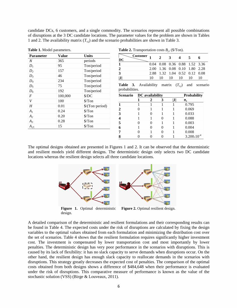
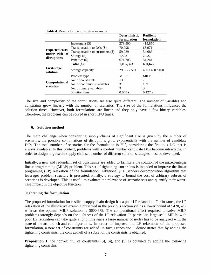
The optimal designs obtained are presented in Figures 1 and 2. It can be observed that the deterministic and resilient models yield different designs. The deterministic design only selects two DC candidate locations whereas the resilient design selects all three candidate locations.

Figure 1. Optimal deterministic design.

Figure 2. Optimal resilient design.

A detailed comparison of the deterministic and resilient formulations and their corresponding results can be found in Table 4. The expected costs under the risk of disruptions are calculated by fixing the design variables to the optimal values obtained from each formulation and minimizing the distribution cost over the set of scenarios. Table 4 shows that the resilient formulation requires significantly higher investment cost. The investment is compensated by lower transportation cost and most importantly by lower penalties. The deterministic design has very poor performance in the scenarios with disruptions. This is caused by its lack of flexibility: it has no slack capacity to serve demands when disruptions occur. On the other hand, the resilient design has enough slack capacity to reallocate demands in the scenarios with disruptions. This strategy greatly decreases the expected cost of penalties. The comparison of the optimal costs obtained from both designs shows a difference of $484,648 when their performance is evaluated under the risk of disruptions. This comparative measure of performance is known as the value of the stochastic solution (VSS) (Birge & Louveaux, 2011).

7

Table 4. Results for the illustrative example.

Deterministic formulation

Resilient formulation

Expected costs under risk of disruptions

Investment ($) 279,900 419,850 Transportation to DCs ($) 70,098 68,971 Transportation to customers ($) 59,029 54,683 Storage ($) 1,593 2,927 Penalties ($) 674,703 54,244 Total ($): 1,085,323 600,675

First-stage solution Storage capacity 298 / - / 501 400 / 400 / 400

Computational statistics

Problem type MILP MILP No. of constraints 13 76 No. of continuous variables 31 199 No. of binary variables 3 3 Solution time 0.058 s 0.127 s

The size and complexity of the formulations are also quite different. The number of variables and constraints grow linearly with the number of scenarios. The size of the formulations influences the solution times. However, both formulations are linear and they only have a few binary variables. Therefore, the problems can be solved in short CPU times.

6. Solution method The main challenge when considering supply chains of significant size is given by the number of scenarios; the possible combinations of disruptions grow exponentially with the number of candidate DCs. The total number of scenarios for the formulation is 2|J|-1, considering the fictitious DC that is always available. In this context, problems with a modest number candidate DCs become intractable. In order to design large-scale supply chains, a number of different solution strategies must be developed. Initially, a new and redundant set of constraints are added to facilitate the solution of the mixed-integer linear programming (MILP) problem. This set of tightening constraints is intended to improve the linear programing (LP) relaxation of the formulation. Additionally, a Benders decomposition algorithm that leverages problem structure is presented. Finally, a strategy to bound the cost of arbitrary subsets of scenarios is developed. This is useful to evaluate the relevance of scenario sets and quantify their worst-case impact in the objective function. Tightening the formulation The proposed formulation for resilient supply chain design has a poor LP relaxation. For instance, the LP relaxation of the illustrative example presented in the previous section yields a lower bound of $420,525, whereas the optimal MILP solution is $600,675. The computational effort required to solve MILP problems strongly depends on the tightness of the LP relaxation. In particular, large-scale MILPs with poor LP relaxation can take quite a long time since a large number of nodes has to be analyzed with the state-of-the-art branch-and-cut algorithms. In order to improve the LP relaxation of the proposed formulation, a new set of constraints are added. In fact, Proposition 1 demonstrates that by adding the tightening constraints, the convex-hull of a subset of the constraints is obtained. Proposition 1: the convex hull of constraints (3), (4), and (5) is obtained by adding the following tightening constraint:

8

𝑦𝑠,𝑗,𝑖,𝑘 − 𝑇𝑠,𝑗𝑥𝑗 ≤ 0 ⩝ s ϵ S, ⩝ j ϵ J, ⩝ i ϵ I,⩝ k ϵ K (6) Proof 1: according to the argument from Geoffrion & Bride (1978) and decomposing the problem by DCs, constraints (3), (4), and (5) can be expressed in disjunctive form as follows:

�𝑥𝑗 = 0 𝑐𝑗,𝑘 = 0𝑦𝑠,𝑗,𝑖,𝑘 = 0

� ∨

⎣⎢⎢⎢⎢⎡

𝑥𝑗 = 10 ≤ 𝑐𝑗,𝑘 ≤ 𝐶𝑚𝑎𝑥

0 ≤ 𝑦𝑠,𝑗,𝑖,𝑘 ≤ 𝑇𝑠,𝑗

�𝐷𝑖,𝑘𝑦𝑠,𝑗,𝑖,𝑘𝑖∈𝐼

≤ 𝑇𝑠,𝑗𝑐𝑗,𝑘⎦⎥⎥⎥⎥⎤

(7)

The MILP hull reformulation is obtained by disaggregating variables xj, cj,k, and ys,j,i,k to obtain the following constraints:

𝑥𝑗1 = 0 𝑥𝑗2 = 1

(8)

𝑐𝑗,𝑘1 = 0 0 ≤ 𝑐𝑗,𝑘

2 ≤ 𝐶𝑚𝑎𝑥

𝑦𝑠,𝑗,𝑖,𝑘1 = 0 0 ≤ 𝑦𝑠,𝑗,𝑖,𝑘

2 ≤ 𝑇𝑠,𝑗

�𝐷𝑖 ,𝑘𝑦𝑠,𝑗,𝑖,𝑘2

𝑖∈𝐼

≤ 𝑇𝑠,𝑗𝑐𝑗,𝑘2

The convex-hull is obtained from the convex combination of the disaggregated variables:

𝑥𝑗 = (1 − 𝛼)𝑥𝑗1 + 𝛼𝑥𝑗2

(9) 𝑐𝑗,𝑘 = 𝑐𝑗,𝑘

1 (1 − 𝛼) + 𝛼𝑐𝑗,𝑘2

𝑦𝑠,𝑗,𝑖,𝑘 = (1 − 𝛼)𝑦𝑠,𝑗,𝑖,𝑘1 + 𝛼𝑦𝑠,𝑗,𝑖,𝑘

2

0 ≤ 𝛼 ≤ 1 Fixing values of 𝑥𝑗1 = 0, 𝑐𝑗,𝑘

1 = 0, and 𝑦𝑠,𝑗,𝑖,𝑘1 = 0 yields:

𝑥𝑗 = 𝛼

(10) 𝑐𝑗,𝑘 = 𝑐𝑗,𝑘2 𝑥𝑗

𝑦𝑠,𝑗,𝑖,𝑘 = 𝑦𝑠,𝑗,𝑖,𝑘2 𝑥𝑗

Substitution in the disaggregated constraints yield:

0 ≤𝑐𝑗,𝑘

𝑥𝑗≤ 𝐶𝑚𝑎𝑥 (11)

0 ≤𝑦𝑠,𝑗,𝑖,𝑘

𝑥𝑗≤ 𝑇𝑠,𝑗 (12)

�𝐷𝑖 ,𝑘𝑦𝑠,𝑗,𝑖,𝑘

𝑥𝑗𝑖∈𝐼

≤ 𝑇𝑠,𝑗𝑐𝑗,𝑘

𝑥𝑗 (13)

0 ≤ 𝑥𝑗 ≤ 1 (14) Constraints (11), (12), (13), and (14) correspond exactly to constraints (2), (4), (6), and the continuous relaxation of (5). □

9

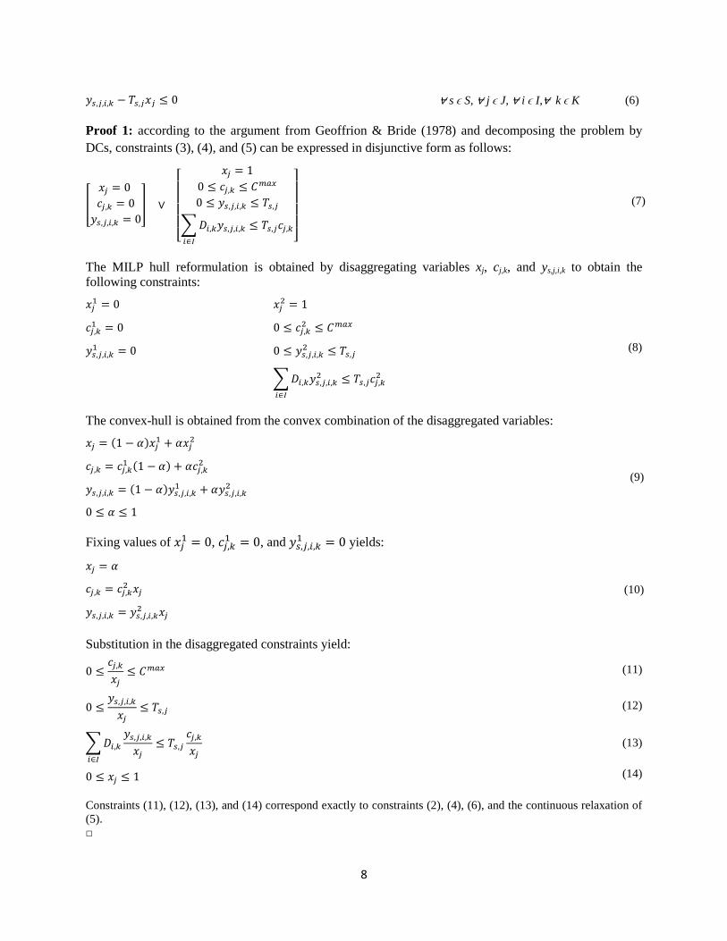
This MILP reformulation is known to yield the convex hull of the disjunctions (Balas, 1979; Raman & Grossmann, 1994). The improvement in the tightness of the LP relaxation can be illustrated with the example presented in the previous section. The addition of the set of tightening constraints (6) to the formulation increases the lower bound from the LP relaxation from $420,525 to $ 589,403; this represents a significant improvement in a problem in which the optimal solution is $600,675. The addition of tightening constraints is important not only for a better LP relaxation of the full problem. The main advantage of this new set of constraints is that it can produce stronger cuts when Benders decomposition is used (Magnanti & Wong, 1981). Multi-cut Benders decomposition Bender decomposition, also known as the L-Shaped method for stochastic programming (Van Slyke & Wets, 1969), is used to avoid the need of solving extremely large problems. This decomposition method finds the optimal value of the objective function by iteratively improving upper and lower bounds on the optimal cost. Upper bounds are found by fixing the first-stage variables and optimizing the second-stage decisions for the scenarios. Lower bounds are found in a master problem that approximates the cost of scenarios in the space of the first-stage variables. The convergence of the algorithm is achieved by improving the lower bounding approximation used in the master problem with the information obtained from the upper bounding subproblems. The main steps of the iterative procedure are shown in Figure 3.

Figure 3. Benders decomposition algorithm The flow of information from subproblems to the master problem is determined by the dual multipliers of the subproblems. The classical approach is to generate one cut in every iteration. Some authors have proposed generating multiple cuts in every iteration (Birge & Louveaux, 1988; Saharidis et al., 2010; You & Grossmann, 2011). Given the structure of the resilient supply chain design problem, there are several possibilities to derive cuts. After different computational experiments it was found that the most efficient

10

strategy is to transfer as much information as possible from the subproblems to the master problem. Therefore, the proposed implementation adds individual cuts per scenario and commodity in every iteration. In the multi-cut framework, the subproblems which can be decomposed by scenario (s ϵ S) and commodity (k ϵ K), are formulated as follows:

min 𝑁�𝜋𝑠����𝐴𝑗,𝑘�𝐷𝑖 ,𝑘𝑦𝑠,𝑗,𝑖,𝑘𝑖∈𝐼

+ �𝐵𝑗 ,𝑖,𝑘𝐷𝑖 ,𝑘𝑦𝑠,𝑗,𝑖,𝑘𝑖∈𝐼

−12𝐻𝑘�𝐷𝑖,𝑘𝑦𝑠,𝑗,𝑖,𝑘

𝑖∈𝐼

�𝑗∈𝐽

�𝑘∈𝐾𝑠∈𝑆

(15)

s.t. � 𝑦𝑠,𝑗,𝑖,𝑘𝐽∈𝐷𝐶

= 1 ⩝ s ϵ S, ⩝ i ϵ I,⩝ k ϵ K (16)

�𝐷𝑖 ,𝑘𝑦𝑠,𝑗,𝑖,𝑘𝑖∈𝐼

− 𝑇𝑠,𝑗𝑐�̅�,𝑘𝑖𝑡𝑒𝑟 ≤ 0 ⩝ s ϵ S, ⩝ j ϵ J, k ϵ K (17)

𝑦𝑠,𝑗,𝑖,𝑘 − 𝑇𝑠,𝑗�̅�𝑗𝑖𝑡𝑒𝑟 ≤ 0 ⩝ s ϵ S, ⩝ j ϵ J, ⩝ i ϵ I,⩝ k ϵ K (18)

𝑦𝑠,𝑗,𝑖,𝑘 ≥ 0 ⩝ s ϵ S, ⩝ j ϵ J, ⩝ i ϵ I,⩝ k ϵ K (19) where �̅�𝑗𝑖𝑡𝑒𝑟 and 𝑐�̅�,𝑘

𝑖𝑡𝑒𝑟 are the optimal first-stage solution of the master problem in the previous iteration (iter-1). The multi-cut master problem is formulated as follows:

min � �𝐹𝑥𝑗 + �𝑉𝑐𝑗,𝑘𝑘∈𝐾

�𝐽∈𝐽\{|𝐽|}

+ 𝑁 � �𝐻𝑘𝑐𝑗,𝑘𝑘∈𝐾𝐽∈𝐽\{|𝐽|}

+ ��𝜃𝑠,𝑘𝑘∈𝐾𝑠∈𝑆

(20)

s.t. 𝜃𝑠,𝑘 ≥ �𝜆𝑠,𝑖,𝑘𝑖𝑡𝑒𝑟 −�𝜇𝑠,𝑗,𝑘

𝑖𝑡𝑒𝑟 𝑇𝑠,𝑗𝑐𝑗,𝑘𝑗∈𝐽𝑖∈𝐼

−��𝛾𝑠,𝑗,𝑖,𝑘𝑖𝑡𝑒𝑟 𝑇𝑠,𝑗𝑥𝑗

𝑖∈𝐼𝑗∈𝐽

⩝ s ϵ S, k ϵ K (21)

𝑐𝑗,𝑘 − 𝐶𝑚𝑎𝑥𝑥𝑗 ≤ 0 ⩝ j ϵ J,⩝ k ϵ K (22)

𝑐𝑗,𝑘 ≥ 0 ; 𝑥𝑗 ∈ �0, 1� ⩝ j ϵ J, ⩝ k ϵ K (23) where 𝜆𝑠,𝑖,𝑘

𝑖𝑡𝑒𝑟 , 𝜇𝑠,𝑗,𝑘𝑖𝑡𝑒𝑟 , 𝛾𝑠,𝑗,𝑖,𝑘

𝑖𝑡𝑒𝑟 are the optimal multipliers associated with set of constraints (16), (17), and (18) respectively in iteration iter. Constraint (21) provides the lower bounding approximation for the cost of satisfying demands of commodity k in scenario s (𝜃𝑠,𝑘). It should be noted that no feasibility cuts are considered since the problem has complete recourse. Strengthening the Benders master problem The multi-cut strategy for Benders decomposition can be very effective to obtain a good approximation of the feasible region in the master problem. However, depending on the number of scenarios and commodities in the instance to be solved, the master problem can become a hard MILP to solve because of the large number of cuts. In order to improve the lower bounds and guide the selection of the first-stage variables, the decisions of the main-scenario (scenario with no disruptions) can be included in the master problem. This formulation of the master problem leverages the significant impact of the main-scenario in the final design given its comparatively high probability. The increase in the size of the master problem when main-scenario decisions are included is modest for problems with a large number of scenarios. The strengthened master problem minimizes the objective function (20) subject to constraints (21), (22), and (23) from the original master problem, and constraints (16), (17), (18), and (19) for the main-scenario.

11

The constraints from the main-scenario subproblem are connected to the objective function through the following constraint:

𝜃1,𝑘 ≥ 𝑁 𝜋𝑠��𝐴𝑗,𝑘�𝐷𝑖 ,𝑘𝑦1,𝑗,𝑖,𝑘𝑖∈𝐼

+ �𝐵𝑗,𝑖,𝑘𝐷𝑖,𝑘𝑦1,𝑗,𝑖,𝑘𝑖∈𝐼

−12𝐻𝑘�𝐷𝑖,𝑘𝑦1,𝑗,𝑖,𝑘

𝑖∈𝐼

�𝑗∈𝐽

k ϵ K (24)

Pareto-optimal cuts Benders subproblems that result from fixing the first-stage decisions are classical transportation problems. These problems are relatively easy to solve but their dual solution is known to be highly degenerate (Wentges, 1996). Therefore, it is very important to select in every iteration a set of optimal multipliers (𝜆𝑠,𝑖,𝑘𝑖𝑡𝑒𝑟 , 𝜇𝑠,𝑗,𝑘

𝑖𝑡𝑒𝑟 , 𝛾𝑠,𝑗,𝑖,𝑘𝑖𝑡𝑒𝑟 ) that produce a strong Benders cut. According to Magnanti & Wong (1981), the best

multipliers for the implementation of Benders decomposition are those that produce non-dominated cuts among the set of optimal multiplies. These cuts are said to be pareto-optimal. Pareto-optimal cuts produce the smallest deviation in the dual objective function value when evaluated at a point (𝑥𝑗0, 𝑐𝑗,𝑘

0 ) in the relative interior of the convex hull of the first-stage variables. Such cuts can be obtained by solving the following linear programming problem:

max ����𝜆𝑠,𝑖,𝑘 −�𝜇𝑠,𝑗,𝑘𝑇𝑠,𝑗𝑐𝑗,𝑘0

𝑗∈𝐽𝑖∈𝐼

−��𝛾𝑠,𝑗,𝑖,𝑘𝑇𝑠,𝑗𝑥𝑗0

𝑖∈𝐼𝑗∈𝐽

�𝑘∈𝐾𝑠∈𝑆

(25)

s.t. 𝑣∗��̅�𝑗𝑖𝑡𝑒𝑟 , 𝑐�̅�,𝑘𝑖𝑡𝑒𝑟� = ����𝜆𝑠,𝑖,𝑘 −�𝜇𝑠,𝑗,𝑘𝑇𝑠,𝑗𝑐�̅�,𝑙

𝑖𝑡𝑒𝑟

𝑗∈𝐽𝑖∈𝐼

−��𝛾𝑠,𝑗,𝑖,𝑘𝑇𝑠,𝑗�̅�𝑗𝑖𝑡𝑒𝑟

𝑖∈𝐼𝑗∈𝐽

�𝑘∈𝐾𝑠∈𝑆

(26)

𝜆𝑠,𝑖,𝑘 − 𝜇𝑠,𝑗,𝑘𝐷𝑖,𝑘 − 𝛾𝑠,𝑗,𝑖,𝑘 ≤ 𝑁 𝜋𝑠 �𝐴𝑗,𝑘 + 𝐵𝑗 ,𝑖,𝑘 −12𝐻𝑘�𝐷𝑖,𝑘 ⩝ s ϵ S, j ϵ J\{|J|}, ⩝ i ϵ I,⩝ k ϵ K (27)

𝜆𝑠,𝑖,𝑘 ≤ 𝑁 𝜋𝑠�𝐴|𝐽|,𝑘 + 𝐵|𝐽|,𝑖,𝑘�𝐷𝑖,𝑘 ⩝ s ϵ S, j ϵ {|J|}, ⩝ i ϵ I,⩝ k ϵ K (28)

𝜆𝑠,𝑖,𝑘 ≥ 0 ; 𝜇𝑠,𝑗,𝑘 ≥ 0; 𝛾𝑠,𝑗,𝑖,𝑘 ≥ 0 ⩝ s ϵ S, j ϵ J, ⩝ i ϵ I,⩝ k ϵ K (29) where 𝑣∗��̅�𝑗𝑖𝑡𝑒𝑟 , 𝑐�̅�,𝑘

𝑖𝑡𝑒𝑟� is the optimal objective value of subproblems at iteration iter and

�𝑥𝑗0, 𝑐𝑗,𝑘0 � ∈ ��𝑥𝑗 , 𝑐𝑗,𝑘�: 0 < 𝑥𝑗 < 1; 0 < 𝑐𝑗,𝑘 < 𝐶𝑚𝑎𝑥𝑥𝑗� (30)

Notice that equation (26) constraints the multipliers to the set of optimizers of the subproblems; inequalities (27), (28), and (29) are the constraints of the dual formulation of subproblems. Bounding the impact of scenario subsets An important observation regarding the problem structure refers to the order of magnitude among different scenario probabilities. Scenarios with increasing number of disrupted locations have smaller probabilities. However, scenarios with the same number of disruptions occurring simultaneously have probabilities on the same order of magnitude. Therefore, the most intuitive way to divide the scenarios is to group them according to the number of simultaneous disruptions. For problems with a large number of scenarios, it is reasonable to select a subset of relevant scenarios (�̂�) for which the optimization problem can be solved, neglecting the effect of the scenarios with very small probabilities. However, solving this reduced problem does not provide much information about the optimal value of the objective function for the cases in which the cost of penalties is very high. Therefore, it is of interest to derive deterministic bounds on the cost of the neglected scenarios.

12

The calculation of the upper bound for the subset of neglected scenarios (�̃�) is based on the implementation of an assignment policy that is always feasible. The proposed policy works as follows. In any given scenario, the main-scenario assignment is attempted for each demand (Di,k): if the assignment is feasible (because the corresponding DC is active) the cost of satisfying the demand equals its cost in the main-scenario, otherwise demand is assumed to be penalized. The proportion in which these two costs are incurred depends on the conditional disruption probabilities of DCs (𝑃𝑗𝑆

�) in the neglected scenarios (�̃�). According to this policy, the upper bound for the cost of neglected scenarios subset (�̃�) can be calculated from equation (31):

𝑈𝐵�̃� = 𝑁 𝛱�̃���1 − 𝑃𝑗�̃��𝐽∈𝐽

���𝐴𝑗,𝑘�𝐷𝑖,𝑘𝑦1,𝑗,𝑖,𝑘 + �𝐵𝑗,𝑖,𝑘𝐷𝑖,𝑘𝑦1,𝑗,𝑖,𝑘𝑖∈𝐼𝑖∈𝐼

+ 𝐻𝑘 �𝑐𝑗,𝑘 −12�𝐷𝑖,𝑘𝑦1,𝑗,𝑖,𝑘𝑖∈𝐼

��𝑘∈𝐾

�

+𝑁 𝛱𝑆��𝑃𝑗𝑆� ���𝐴|𝐽|,𝑘�𝐷𝑖,𝑘𝑦1,𝑗,𝑖,𝑘 + �𝐵|𝐽|,𝑖,𝑘𝐷𝑖,𝑘𝑦1,𝑗,𝑖,𝑘

𝑖∈𝐼𝑖∈𝐼

+ 𝐻𝑘𝑐𝑗,𝑘�𝑘∈𝐾

�𝐽∈𝐽

(31)

where 𝛱𝑆� = ℙ�𝑆�� is the probability of the subset of neglected scenarios �̃�, 𝑃𝑗𝑆

� is the conditional probability of disruption at DC j in subset of scenarios �̃�, 𝑦1,𝑗,𝑖,𝑘 are the main-scenario assignments, and 𝐴|𝐽|,𝑘 and 𝐵|𝐽|,𝑖,𝑘 determine the unit cost for unsatisfied demand Di,k. Therefore, the first term in (31) corresponds to the cost of the feasible assignments in subset (�̃�) and the second term corresponds to penalties for infeasible assignments in subset (�̃�). The calculation of the conditional probability of disruption in scenario subset �̃� is based on the assumption that disruptions at DCs are independent from each other. Figure 4 shows the scenario subsets and the relationship between their probabilities. Proposition 2 formalizes the procedure to calculate the conditional probability of disruption (𝑃𝑗𝑆

�) in the subset of neglected scenarios (�̃�).

Figure 4. Scenario subsets and their probabilities Proposition 2: for the set of scenarios (S) generated by assuming independent DC disruption probabilities, the conditional probability of finding DC j disrupted in subset of scenarios �̃� can be calculated from the conditional probability of finding DC j disrupted in its complement (�̃� 𝐶) and the overall disruption probability of DC j in S.

ℙ�𝑆𝑗|�̃� � =ℙ�𝑆𝑗� − ℙ��̃� � ∗ ℙ�𝑆𝑗|�̃� 𝐶�

ℙ��̃�� (32)

Where 𝑆𝑗 denotes the scenarios in which DC j is disrupted, �̃� denotes the realization of a scenario 𝑠 ⊂ �̃� and �̃�𝐶 is its complement.

13

Proof 2: by definition

ℙ�𝑆𝑗|�̃�� =ℙ�𝑆𝑗 ∩ �̃��ℙ��̃��

(33)

ℙ�𝑆𝑗|�̃�𝐶� =ℙ�𝑆𝑗 ∩ �̃�𝐶�ℙ��̃�𝐶�

Since �̃�and �̃�𝐶 are the complements of each other:

ℙ�𝑆𝑗� = ℙ��𝑆𝑗 ∩ �̃�� ∪ �𝑆𝑗 ∩ �̃�𝐶�� (34)

ℙ�𝑆𝑗� = ℙ��̃�� ∗ ℙ�𝑆𝑗|�̃�� + ℙ��̃�� ∗ ℙ�𝑆𝑗|�̃�𝐶� (35)

It must be noted that equation (35) is equivalent to equation (32).

□ Analogously, a lower bound on the cost of subset of scenarios �̃� can be calculated by assuming that all demands can be satisfied from the DC assigned in the main-scenario as presented in equation (36).

𝐿𝐵�̃� = 𝑁 𝛱�̃���� �𝐴𝑗,𝑘�𝐷𝑖,𝑘𝑦1,𝑗,𝑖,𝑘 + �𝐵𝑗 ,𝑖,𝑘𝐷𝑖,𝑘𝑦1,𝑗,𝑖,𝑘𝑖∈𝐼𝑖∈𝐼

+ 𝐻𝑘 �𝑐𝑗,𝑘 −12�𝐷𝑖,𝑘𝑦1,𝑗,𝑖,𝑘𝑖∈𝐼

��𝑘∈𝐾

�𝐽∈𝐽

(36)

7. Implementation The proposed solution method is implemented in GAMS 24.1.1 for a large-scale and an industrial case study. All problems are solved using GUROBI 5.5.0 in an Intel Xeon CPU (12 cores) 2.67 GHz with 16 GB of RAM. In order to speed-up the solution time, a number of problem specific properties can be leveraged.

• Undistinguishability: the upper bound for a particular design is evaluated in the Benders subproblems. Scenarios that are only different from each other because of disruptions at locations that are not selected (�̅�𝑗𝑖𝑡𝑒𝑟 = 0) become undistinguishable. All the scenarios in these sets have the same optimal solution. Therefore, it is enough to solve one of the undistinguishable scenarios and use the solution for all the scenarios in the set.

• Parallelization: the upper bounding subproblems are completely independent of each other with respect to scenarios and commodities. They can be solved in parallel using GAMS grid computing. The degree of parallelization must balance the time required to start the executions, solve the subproblems, and read the solutions. For the large-scale instances studied in this paper, the highest efficiency was found by solving for all commodities at the same time in individual scenarios.

• Relevance of scenarios: the total number of scenarios grows exponentially with the number of candidate DCs. If all possible scenarios are considered, it is impossible to find the optimal design of industrial supply chains with the current computational technology. However, most of the scenarios that can be generated have very small probabilities. The magnitude of the scenario probabilities are directly related to the number of disruptions occurring at the same time. Therefore, it is easy to identify a reduced subset of relevant scenarios whose optimal solution is a good approximation of the full-space solution.

• Full-space bounds: bounds on the cost of scenarios excluded from the optimization problem can be calculated from (31) and (36). Upper and lower bounds on the full-space problem can be calculated by adding the bounds obtained for the relevant set of scenarios through Benders

14

decomposition to the bounds obtained from (31) and (36) for scenarios excluded from the optimization problem.

The sequence in which the proposed solution method is implemented is presented in figure 5.

Figure 5. Implementation sequence of solution method.

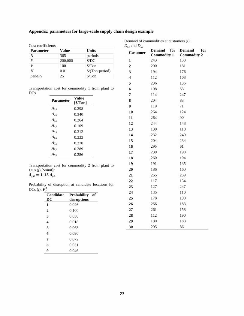
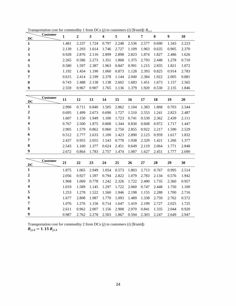
8. Large-scale example The solution strategy developed in the previous sections is used to solve a large-scale supply chain design problem with risk of disruptions at candidate DC locations. The parameters of the problem were generated randomly; they are presented in the Appendix. The problem includes: 1 production plant, 9 candidate locations for DCs, and 30 customers with demands for 2 commodities. The candidate DCs have disruption probabilities between 2% and 10%. The number of scenarios in the full-space problem is 29 =

15

512. The design is based on a time-horizon (N) of 365 days; in this time-scale, investment cost can be interpreted as annualized cost. The instance is used to illustrate the use of Benders decomposition, the benefits of strengthening the master problem, and the impact of solving a reduced subset of relevant scenarios. The selected relevant subset of scenarios includes scenarios with up to 4 simultaneous disruptions, for a total of 256 scenarios with probability ( 𝛱�̂�) equal to 99.99%. A comparison of the results for the full-space problem and the reduced problem is shown in Table 5.

Table 5. Expected costs for the large-scale supply chain design obtained from full-space and reduced instances. Expected cost Full-space instance Reduced instance Investment ($): 2,194,100 2,194,100 Transportation to DCs ($): 936,260 936,238 Transportation to customers ($): 3,615,300 3,615,209 Storage ($): 319,440 319,429 Penalties ($): 160,347 159,615 Total ($): 7,225,447 7,224,591 Full-space upper bound: 7,225,447 7,225,898 Full-space lower bound: 7,225,447 7,224,728

The results show that solutions obtained for the full-space and the reduced problem are very similar. In particular, their optimal solutions imply the same design decisions and therefore the same investment cost. It is interesting to note that the largest difference in the results appears in the expected cost of penalties. This result is reasonable because the scenarios that are ignored in the reduced problem are expected to be expensive in terms of penalties. Both problems were solved to 0% optimality tolerance using the proposed Benders decomposition algorithms. The solution obtained for the full-space problem establishes with certainty the optimal solution because all the scenarios are included in the optimization problem. The solution obtained for the reduced problem establishes a lower bound on the full-space optimum because it neglects the effect of some scenarios. When the bounds on the full-space problem are calculated from equations (31) and (36), it can be observed that they yield a very tight approximation of the full-space solution with an optimality gap less than 0.1%. The size of the optimization instances and their solution times are shown in Table 6.

Table 6. Instance sizes and solution times Model statistic Full-space instance Reduced instance Number of constraints: 318,479 159,247 Number of continuous variables: 309,263 154,639 Number of binary variables: 9 9 Number of multi-cut Benders iterations: 15 15 Multi-cut Benders solution time: 281 s 151 s Strengthened multi-cut Benders solution time: 176 s 89 s Number of strengthened multi-cut Benders iterations: 8 8

It can be observed that the reduced problem is almost half the size of the full-space problem in terms of constraints and continuous variables. This is explained by the reduction in the number of scenarios. The solution time for both instances reduces in a smaller proportion because the algorithms spend most of the

16

time solving the MILP master problems. The use of the strengthened multi-cut master problem further reduces the solution time because it implies fewer iterations as shown in Figure 6. In general, it has been found that the proposed strategy is effective to solve a large-scale instance of high computational complexity.

Figure 6. Convergence of Benders algorithms for the full-space instance of the large-scale example

9. Industrial supply chain design The proposed model and solution strategy is used for the optimal design of an industrial supply chain with risk of disruption at candidate DCs. The problem includes: 1 production plant, 29 candidate locations for DCs, 110 customers, and 61 different commodities. Not all the customers have demand for all commodities; there are a total of 277 demands for commodities in every time-period. The DC candidate locations have independent probabilities of being disrupted between 0.5% and 3%. The number of scenarios in the full-space problem is 229, approximately 537 million. The magnitude of penalties for unsatisfied demand is around 10 times the highest distribution cost among all possible assignments. The design is based on a time-horizon (𝑁) of 60 months. The specific data for this instance is not disclosed for confidentiality reasons. Three subsets of scenarios are used for the design of the industrial supply chain. The first reduced problem only includes the main-scenario and it is equivalent to the deterministic formulation of the supply chain design problem. The second reduced problem considers the main-scenario and the scenarios with one disruption. The third reduced problem includes the scenarios with up to 2 simultaneous disruptions. Table 7 shows the problem sizes for the different instances. It can be observed that the third instance, in which the scenarios comprise 98.5% of the possible realizations, is a very challenging problem in terms of size.

17

Table 7. Instances of the industrial design with increasing number of maximum simultaneous disruptions Maximum simultaneous disruptions

Number of scenarios in subset

Probability of subset

Number of constraints

Number of continuous variables

Number of discrete variables

0 1 0.590 11,854 10,085 29 1 30 0.905 304,261 251,191 29 2 436 0.985 4,397,989 3,626,675 29

The first instance was solved directly without decomposition. The second and third instances were solved using the strengthened multi-cut Benders decomposition. The results obtained are shown in Table 8.

Table 8. Upper and lower bounds for instances of the industrial design. Reduced

problem 0 Reduced problem 1

Reduced problem 2

Optimal investment ($) 18.47 18.77 21.01 Number of selected DCs: 1 4 12 Instance upper bound ($): 34.09 48.68 53.66 Instance lower bound ($): 34.09 48.30 53.25 Instance optimality gap: 0% 0.78% 0.77% Number of Benders iterations: - 4 6 Solution time: 0.1 min 84.03 min 1,762 min Full-space upper bound: 57.41 56.31 55.59 Full-space lower bound: 48.15 52.87 53.67

It can be observed that the investment cost has a modest increase when the model includes a larger number of adverse scenarios. In this case, the formulation leverages the complexity of the supply chain network by decentralizing inventories at a relative low cost. This strategy avoids costly demand penalties and improves supply chain resilience. The full-space bounds obtained from equations (31) and (36) for the different instances show the importance of considering a relevant subset of scenarios that provides a good representation of the full-space problem. The solution obtained from Reduced problem 0 can only guarantee the total cost to be within a 16.13% difference of the optimal cost. On the other hand, the solution obtained from Reduced problem 2 yields a total cost that in the worst case would be 3.5% higher than the optimal cost. The computational effort to solve the larger instances of the industrial supply chain design is very significant. Even after applying the strategy developed in the previous sections, it takes a long time to find satisfactory solutions. In this example, the number of scenarios and commodities implies a large number of cuts in the Benders master problem. The complexity of the MILP master problem increases very rapidly with iterations. Fortunately, the algorithm converges after few iterations.

10. Conclusions The design of resilient supply chains has been formulated as a two-stage stochastic programming problem to include the risk of disruptions at DC. The model allows finding the design decisions that minimize investment and expected distribution cost over a finite time-horizon by anticipating the distribution strategy in different scenarios. The allocation of inventory at DCs plays a critical role in supply chain resilience since it allows flexibility for the satisfaction of customers’ demands in different scenarios. This strategy contradicts the generalized trend to centralize distribution centers and reduce inventories. The examples show that resilient supply chain designs can be obtained with reasonable increases in

18

investment costs. These increased investments are compensated by lower transportation costs and better performance in the scenarios with disruptions. The main challenge for the design of resilient large-scale supply chains originates from the exponential growth in the number of scenarios as a function of the number of DC candidate locations. Different strategies have been developed to exploit the problem structure. The importance of a tight MILP formulation has been illustrated. The multi-cut version of Benders decomposition has been adapted to leverage the particular problem structure. In order to reduce the number of iterations, pareto-optimal cuts were added to the master problem for every commodity in each scenario. Additionally, including the assignment decisions of the main-scenario in the Benders master problem was found to reduce the number of iterations and the computational time. For large-scale problems, the optimization over reduced number scenarios yielded good approximations of the optimal design. Furthermore, the implementation of a distribution policy in the scenarios with very small probabilities has allowed finding deterministic bounds on the performance of the supply chain. The solution strategy has been used to design a multi-commodity industrial supply chain. The economic benefits of considering resilience in supply chain design have been demonstrated. The implementation of resilient designs has the potential to improve supply chain performance and reduce their vulnerability to unexpected events. Acknowledgements The authors gratefully acknowledge the financial support from the Fulbright program and the Dow Chemical Company.

19

References

Balas, E. (1979). Disjunctive Programming, Annals of Discrete Mathematics 5, 3-51.

Benders, J.F.(1962). Partitioning procedures for solving mixed-variables programming problems. Numerische Mathematik, 4, 238-252.

Berk, E. & Arreola-Risa, A. (1994). Note on "Future supply uncertainty in EOQ models". Naval Research Logistics, 41, 129-132.

Bhatia, G.; Lane, C. & Wain, A. (2013). Building Resilience in Supply Chains. World Economic Forum. An Initiative of the Risk Response Network in collaboration with Accenture.

Birge, J.R. & Louveaux, F.V. (1988). A multicut algorithm for two-stage stochastic linear programs. European Journal of Operational Research, 34, 384-392.

Chen, Q.; Li, X.; Ouyang, Y. (2011). Joint inventory-location problem under the risk of probabilistic facility disruptions. Transportation Research Part B: Methodological, 45, 991-1003.

Chopra, S. & Sodhi, M.S. (2004). Managing risk to avoid supply-chain breakdown. MIT Sloan Management Review, 46, 52-61.

Coullard, C.; Daskin, M.S. (2003). A Joint Location-Inventory Model. Transportation Science, 37, 40-55.

Craighead, C. & Blackhurst, J. (2007). The Severity of Supply Chain Disruptions: Design Characteristics and Mitigation Capabilities. Decision Sciences, 38, 131-156.

Cui, T.; Ouyang, Y. & Shen, Z-J.M. (2010). Reliable Facility Location Design under the Risk of Disruptions. Operations Research, 58, 998-1011.

Daskin, M. S.; Coullard, C. R. & Shen, Z. J. M. (2002). An Inventory-Location Model: Formulation, Solution Algorithm and Computational Results. Annals of Operations Research, 110, 83-106.

Eppen, G.D. (1979). Effects of Centralization on Expected Costs in a Multi-Location Newsboy Problem. Management Science, 25, 498-501.

Geoffrion A. & McBride R. (1978). Lagrangean Relaxation Applied to Capacitated Facility Location Problems. IIE Transactions, 10, 40-47.

Geoffrion, A.M.; Graves, G.W. (1974). Multicomodity distribution system design by Benders Decomposition. Management Science, 20, 822-844.

Goel, V. & Grossmann, I.E. (2006). A Class of stochastic programs with decision dependent uncertainty. Mathematical Programming, 108, 355-394.

Gupta, V. & Grossmann, I.E. (2011). Solution strategies for multistage stochastic programming with endogenous uncertainties. Computers & Chemical Engineering, 35, 2235-2247.

20

Helferich, O.K. & Cook, R.L. (2002). Securing the Supply Chain. Council of Logistics Management (CLM).

J. Birge & F. Louveaux. Introduction to stochastic programming (2nd Ed.). Springer, New York, 2011.

Jeon, H-M. (2011). Location-Inventory Models with Supply Disruptions. ProQuest, UMI Dissertation Publishing.

Jonsbraten, T.W.; Wets, R.J.B. & Woodruff, D.L.(1998). A class of stochastic programs with decision dependent random elements. Annals of Operations Research, 82, 83-106.

Kleywegt, A.J.; Shapiro, A. & Homem de Mello, T. (2001). The sample average approximation method for stochastic discrete optimization. SIAM Journal of Optimization, 12, 479-502.

Klibi, W. & Martel, A. (2012a). Modeling approaches for the design of resilient supply chain networks under disruptions. International Journal of Production Economics, 135, 882-898.

Klibi, W. & Martel, A. (2012b). Scenario-based Supply Chain Network risk modeling. European Journal of Operational Research, 223, 644-658.

Klibi, W.; Martel, A. & Guitouni, A. (2010). The design of robust value-creating supply chain networks: A critical review. European Journal of Operations Research 203, 283-293.

Krausmann, E. & Cruz, A.M. (2013). Impact of the 11 March 2011, Great East Japan earthquake and tsunami on the chemical industry. Natural Hazards, 67, 811-828.

L.V. Snyder. (2006). Facility location under uncertainty: A review. IIE Transactions, 38, 547-564.

Latour, A. (2001). Trial by fire: A blaze in Albuquerque sets off major crisis for cell-phone giants. Wall Street Journal (January 29).

Li, Q. Zeng, B. & Savachkin, A. (2013). Reliable facility location design under disruptions. Computers & Operations Research, 40, 901-909.

Li, X. & Ouyang, Y. (2010). A continuum approximation approach to reliable facility location design under correlated probabilistic disruptions. Transportation Research Part B: Methodological, 44, 535-548.

Lim, M.; Daskin, M.S.; Bassamboo, A. & Chopra, S. (2010). A facility reliability problem: Formulation, properties, and algorithm. Naval Research Logistics, 57, 58-70.

Magnanti, T.L. & Wong R.T. (1981). Accelerating Benders Decomposition: Algorithmic Enhacement and Model Selection Criteria. Operations Research, 29, 464-484.

Meixell, M. J. & Gargeya, V. B. (2005). Global supply chain design: A literature review and critique. Transportation Research Part E: Logistics and Transportation Review, 41, 531-550.

Nwazota, K. (2005). Hurricane Katrina Underscores Tenuous State of U.S. Oil Refining Industry. Oneline NewsHour (September 9).

21

Owen, S.H.; Daskin, M.S. (1998). Strategic facility location: A review. European Journal of Operational Research, 111, 423-447.

Parlar, M. & Berkin, D. (1991). Future supply uncertainty in EOQ models. Naval Research Logistics, 38, 107-121.

Peng, P. ; Snyder, L.V.; Lim, A. & Liu, Z. Reliable logistics networks design with facility disruptions. Transportation Research Part B: Methodological, 45, 1190-1211.

Qi, L.; Shen, Z-J.M. & Snyder, L.V. (2009). A Continuous-Review Inventory Model with Disruptions at Both Supplier and Retailer. Production and Operations Management, 18, 516-532.

Qi, L.; Shen, Z-J.M. & Snyder, L.V. (2010). The Effect of Supply Disruptions on Supply Chain Design Decisions. Transportation Science, 44, 274-289.

Raman, R. & I.E. Grossmann. (1994). Modelling and Computational Techniques for Logic Based Integer Programming. Computers & Chemical Engineering, 18, 563-578.

Rice, J. & Caniato, F. (2003). Building a secure and resilient supply chain network. Supply Chain Management Review (September/October), 22-30.

Saharidis, G.K.; Minoux, M. & Ierapetritou, M.G. (2010). Accelerating Benders decomposition using covering cut bundle generation. International Transactions in Operational Research, 17, 221-237.

Santoso, T.; Ahmed, S.; Goetschalckx, M. & Shapiro, A. (2005). A stochastic programming approach for supply chain network design under uncertainty. European Journal of Operational Research 167, 96-115.

Schütz, P. & Tomasgard, A. (2011). The impact of flexibility on operational supply chain planning. International Journal of Production Economics, 134, 300-311.

Shah, N. (2005). Process industry supply chains: Advances and challenges. Computers and Chemical Engineering, 29, 1225-1235.

Shapiro, A. & Homem de Mello, T. (1998). A simulation-based approach to stochastic programming with recourse. Mathematical Programming, 81, 301-325.

Shen, Z-J.M. (2007). Integrated Supply Chain Design Models: A survey and Future Research Direction. Journal of Industrial and Management Optimization, 3, 1-27.

Shen, Z-J.M.; Zhan, R.L. & Zhang, J. (2011). The Reliable Facility Location Problem: Formulations, Heuristics, and Approximation Algorithms. INFORMS Journal on Computing, 23, 470-482.

Shutz, P.; Tomasgard, A. & Ahmed, S. 2009. Supply chain design under uncertainty using sample average approximation and dual decomposition. European Journal of Operations Research, 199, 409-419.

Snyder L.V.; Shen, Z.-J. (2011). Fundamentals of Supply Chain Theory. John Wiley & Sons, Hoboken (NJ), pp. 63-116.

22

Snyder, L.V. & Daskin, M.S. (2005). Reliability Models for Facility Location: The Expected Failure Cost Case. Transportation Science, 39, 400-416.

Snyder, L.V.; Shen, Z-J.M. (2006). Supply and demand uncertainty in multi-echelon supply chains. Unpublished. College of Engineering and Applied Sciences, Lehigh University.

Tomlin, B. (2006). On the value of mitigation and contingency strategies for managing supply chain disruptions risk. Management Science, 52, 639-657.

Tsiakis, P.; Shah, N. & Pantelides, C. (2001). Design of Multi-echelon Supply Chain Networks under Demand Uncertainty. Industrial & Engineering Chemistry Research, 40, 3585-3604.

Van Slyke, R.M. & Wets, R. (1969). L-Shaped Linear Programs with Applications to Optimal Control and Stochastic Programming. SIAM Journal on Applied Mathematics, 17, 638-663.

Weber, A.; Friedrich, C.J. (1929). Alfred Weber's theory of the location of industries. Chicago: The University of Chicago Press.

Wentges, P. (1996). Accelerating Benders' decomposition for the capacitated facility location problem. Mathematical Methods of Operations Research, 44, 267-290.

You, F. & Grossmann I.E. (2011). Multicut Benders decomposition algorithm for process supply chain planning under uncertainty. Annals of Operations Research.

You, F. & Grossmann, I. E. (2008). Mixed-Integer Nonlinear Programming Models and Algorithms for Large-Scale Supply Chain Design with Stochastic Inventory Management. Industrial & Engineering Chemistry Research, 47, 7802-7817.

23

Appendix: parameters for large-scale supply chain design example Cost coefficients

Demand of commodities at customers (i): Di,1 and Di,2

Parameter Value Units 𝑁 365 periods F 200,000 $/DC V 100 $/Ton H 0.01 $/(Ton·period) penalty 25 $/Ton

Customer Demand for Commodity 1

Demand for Commodity 2

1 243 133 2 200 181 3 194 176 4 112 108 5 236 136 6 108 53 7 114 247 8 204 83 9 119 71 10 264 124 11 264 90 12 244 148 13 130 118 14 232 240 15 204 234 16 295 61 17 230 198 18 260 104 19 191 135 20 186 160 21 265 239 22 117 134 23 127 247 24 135 110 25 178 190 26 266 183 27 261 158 28 112 190 29 180 183 30 205 86

Transportation cost for commodity 1 from plant to DCs

Parameter Value [$/Ton]

A1,1 0.298 A2,1 0.340 A3,1 0.264 A4,1 0.109 A5,1 0.312 A6,1 0.333 A7,1 0.270 A8,1 0.289 A9,1 0.286

Transportation cost for commodity 2 from plant to DCs (j) [$/unit]: 𝑨𝒋,𝟐 = 𝟏.𝟏𝟓 𝑨𝒋,𝟏

Probability of disruption at candidate locations for DCs (j): 𝑷𝒋𝟎

Candidate DC

Probability of disruptions

1 0.026 2 0.100 3 0.030 4 0.018 5 0.063 6 0.090 7 0.072 8 0.031 9 0.046

24

Transportation cost for commodity 1 from DCs (j) to customers (i) [$/unit]: Bj,i,1 Customer 1 2 3 4 5 6 7 8 9 10 DC 1 1.481 2.237 1.724 0.797 2.248 2.536 2.577 0.690 1.343 2.223 2 2.139 1.293 1.614 1.746 2.727 1.109 1.963 0.635 0.905 2.370 3 0.928 2.876 2.116 2.899 2.898 2.823 1.874 1.827 2.486 1.626 4 2.265 0.586 2.273 1.351 1.868 1.375 2.793 2.448 1.278 0.710 5 0.580 1.597 2.387 1.963 0.847 0.991 1.215 2.835 1.821 1.072 6 1.192 1.454 1.190 1.060 0.873 1.128 2.393 0.825 0.914 2.783 7 0.615 2.414 2.199 2.378 1.144 2.040 2.384 1.922 2.005 0.881 8 0.743 2.488 2.138 1.138 2.602 1.683 1.451 1.673 1.157 2.565 9 2.559 0.967 0.907 1.765 1.136 1.379 1.920 0.530 2.135 1.846 Customer 11 12 13 14 15 16 17 18 19 20 DC 1 2.990 0.711 0.840 1.505 2.862 1.104 1.383 1.868 0.703 2.544 2 0.695 1.499 2.673 0.690 1.727 1.510 2.553 1.241 2.823 2.487 3 1.607 1.150 1.949 1.100 1.723 0.741 0.539 2.362 2.439 2.111 4 0.767 2.500 1.875 0.808 1.344 0.830 0.608 0.972 1.717 1.447 5 2.905 1.579 0.862 0.960 2.750 2.855 0.922 2.217 1.590 2.529 6 0.512 2.777 2.633 1.100 1.423 2.890 2.123 0.959 1.617 1.832 7 2.437 0.955 2.055 1.543 0.778 1.938 2.329 1.421 1.266 1.377 8 2.543 1.160 1.377 0.624 2.451 0.649 2.119 2.064 1.771 2.848 9 2.672 0.864 1.783 2.757 1.474 1.087 1.627 2.451 1.777 2.690 Customer 21 22 23 24 25 26 27 28 29 30 DC 1 1.875 1.065 2.949 1.054 0.573 1.803 2.713 0.767 0.995 2.514 2 2.056 0.927 1.597 0.794 2.822 1.079 2.783 2.134 0.576 1.942 3 1.968 1.069 0.778 1.242 2.326 1.722 2.490 1.735 2.360 0.957 4 1.019 1.589 1.145 1.297 1.722 2.060 0.747 2.448 1.750 1.100 5 1.253 1.278 1.522 1.560 1.946 2.198 1.155 2.288 1.700 2.716 6 1.677 2.808 1.987 1.770 1.093 1.489 1.338 2.759 2.762 0.572 7 1.076 1.576 1.156 0.714 1.647 1.419 2.199 2.727 2.025 1.725 8 2.611 0.962 2.007 1.156 2.908 2.970 0.841 1.335 2.044 0.920 9 0.987 2.762 2.278 2.503 1.867 0.594 2.303 2.247 2.649 2.947 Transportation cost for commodity 2 from DCs (j) to customers (i) [$/unit]: 𝑩𝒋,𝒊,𝟐 = 𝟏.𝟏𝟓 𝑩𝒋,𝒊,𝟏