design of fuzzy neural network for function approximation ... · pdf filedesign of fuzzy...

Design of Fuzzy Neural Network for FunctionApproximation and Classification

Amit Mishra, Zaheeruddin ∗†

Abstract— A hybrid Fuzzy Neural Network (FNN)

system is presented in this paper. The proposed

FNN can handle numeric and fuzzy inputs simulta-

neously. The numeric inputs are fuzzified by input

nodes upon presentation to the network while the

fuzzy inputs do not require this translation. The

connections between input to hidden nodes repre-

sent rule antecedents and hidden to output nodes

represent rule consequents. All the connections are

represented by Gaussian fuzzy sets. The mutual

subsethood measure for fuzzy sets that indicates

the degree to which the two fuzzy sets are equal

and is used as a method of activation spread in the

network. A volume based defuzzification method is

used to compute the numeric output of the network.

The training of the network is done using gradient

descent learning procedure. The model has been

tested on three benchmark problems i.e. sine−cosine

and Narazaki Ralescu’s function for approximation

and Iris flower data for classification. Results are also

compared with existing schemes and the proposed

model shows its natural capability as a function

approximator, and classifier.

Keywords: Cardinality, classifier, function ap-

proximation, fuzzy neural system, mutual subsethood

1 Introduction

The conventional approaches to system modeling that arebased on mathematical tools (i.e. difference equations)perform poorly in dealing with complex and uncertainsystems. The basic reason is that, most of the time; it isvery difficult to find a global function or analytical struc-ture for a nonlinear system. In contrast, fuzzy logic pro-vides an inference morphology that enables approximatehuman reasoning capability to be applied in a fuzzy infer-ence system. Therefore, a fuzzy inference system employ-ing fuzzy logical rules can model the quantitative aspectsof human knowledge and reasoning processes without em-ploying precise quantitative analysis.

∗Jaypee Institute of Engineering and Technology, A.B. Road,Raghogarh, Distt.Guna, Madhya Pradesh, India, PIN-473226.Email: amitutk@ gmail.com

†Jamia Millia Islamia (A Central University), Department ofElectrical Engineering, Jamia Nagar, New Delhi, India, PIN-110025. Email: zaheer 2k@ hotmail.com

In recent past, artificial neural network has also playedan important role in solving many engineering problems[1], [2]. Neural network has advantages such as learning,adaption, fault tolerance, parallelism, and generalization.The fuzzy system utilizing the learning capability of neu-ral networks can successfully construct the input outputmapping for many applications [3], [4]. The benefits ofcombining fuzzy logic and neural network have been ex-plored extensively in the literature [5], [6], [7], [8], [9].The term neuro-fuzzy system (also neuro-fuzzy methodsor models) refers to combinations of techniques from neu-ral networks and fuzzy system [10], [11], [12], [13], [14].This does not mean that a neural network and a fuzzysystem are used in some kind of combination, but a fuzzysystem is created from data by some kind of (heuristic)learning method, motivated by learning procedures usedin neural networks. The neuro-fuzzy methods are usuallyapplied, if a fuzzy system is required to solve a problemof function approximation−or a special case of it, like,control or classification [15], [16], [17], [18], [19]−and theotherwise manual design process should be supported andreplaced by an automatic learning process.In this paper, the attention has been focused on the func-tion approximation and classification capabilities of thesubsethood based fuzzy neural model (subsethood basedFNN). This model can handle simultaneous admissionof fuzzy or numeric inputs along with the integration ofa fuzzy mutual subsethood measure for activity propa-gation. A product aggregation operator computes thestrength of firing of a rule as a fuzzy inner product andworks in conjunction with volume defuzzification to gen-erate numeric outputs. A gradient descent algorithm al-lows the model to fine tune rules with the help of numericdata.The organization of the paper is as follows: Section 2presents the architectural and operational detail of themodel. Section 3 describes the gradient descent learningprocedure for training the model. Section 4 and Section 5shows the experiment results for three benchmark prob-lems based on function approximation and classification.Finally, the Section 6 concludes the paper.

2 Fuzzy Neural Network system

The proposed architecture of subsethood based Fuzzyneural network is shown in Fig. 1. Here x1 to xm and

IAENG International Journal of Computer Science, 37:4, IJCS_37_4_02

(Advance online publication: 23 November 2010)

______________________________________________________________________________________

x1

xi

xm

xm+1

xn

Input Layer Rule Layer Output Layer

Numeric nodes

Linguistic nodes

y1

yk

yp

(cij, σij)

(cnj, σnj)

(cjk, σjk)

(cqk, σqk)

Antecedent connection

consequent connection

Figure 1: Architecture of subsethood based FNN model.

xm+1 to xn are numeric and linguistic inputs respectively.Each hidden node represents a rule, and input-hiddennode connection represents fuzzy rule antecedent. Eachhidden-output node connection represents a fuzzy ruleconsequent. Fuzzy set corresponding to linguistic levelsof fuzzy if-then rules are defined on input and outputUODs and are represented by symmetric Gaussian mem-bership functions specified by a center c and spread σ.The center and spread of fuzzy weights wij from inputnodes i to rule nodes j are shown as cij and σij of aGaussian fuzzy set and denoted by wij = (cij , σij). In asimilar way, consequent fuzzy weights from rule nodes jto output nodes k are denoted by vjk = (cjk, σjk). Herey1 to yk . . . yp are the outputs of the subsethood basedFNN model.

2.1 Signal Transmission at Input Nodes

In the proposed FNN the input features x1, ..., xn can beeither linguistic or numeric or the combination of both.Therefore two kinds of nodes may present in the inputlayer of the network corresponding to the nature of inputfeatures.Linguistic nodes accept the linguistic inputs representedby a fuzzy sets with a Gaussian membership function andmodeled by a center ci and spread σi. These linguistic in-puts can be drawn from pre-specified fuzzy sets as shownin Fig. 2, where three Gaussian fuzzy sets have been de-fined on the universe of discourse (UODs) [-1,1]. Thus,a linguistic input feature xi is represented by the pair ofcenter and spread (ci, σi). No transformation of inputstakes place at linguistic nodes in the input layer. Theymerely transmit the fuzzy input forward along antecedentweights.Numeric nodes accept numeric inputs and fuzzify theminto Gaussian fuzzy sets. The numeric input is fuzzi-fied by treating it as the centre of a Gaussian member-ship function with a heuristically chosen spread. An ex-ample of this fuzzification process is shown in Fig. 3,where a numeric feature value of 0.3 has been fuzzified

-1 -0.5 0 0.5 10

0.1

0.2

0.3

0.4

0.5

0.6

0.7

0.8

0.9

1

LOW MEDIUM HIGH

Figure 2: Fuzzy sets for fuzzy inputs.

-1 -0.5 0 0.5 10

0.1

0.2

0.3

0.4

0.5

0.6

0.7

0.8

0.9

1

Fuzzified input Gaussian m.f. Center=0.3Spread=0.35

Figure 3: Fuzzification of numeric input.

into a Gaussian membership function centered at 0.3 withspread 0.35. The Gaussian shape is chosen to match theGaussian shape of weight fuzzy sets since this facilitatessubsethood calculations detailed in section 2.2.Therefore, the signal from a numeric node of the inputlayer is represented by the pair (ci, σi). Antecedent con-nections uniformly receive signals of the form (ci, σi).Signals (S(xi) = (ci, σi)) are transmitted to hidden rulenodes through fuzzy weights wij also of the form (cij , σij),where single subscript notation has been adopted for theinput sets and the double subscript for the weight sets.

2.2 Signal Transmission from Input to RuleNodes (Mutual Subsethood Method)

Since both the signal and the weight are fuzzy sets, beingrepresented by Gaussian membership function, there is aneed to quantify the net value of the signal transmittedalong the weight by the extent of overlap between the twofuzzy sets. This is measured by their mutual subsethood[20]. Consider two fuzzy sets A and B with centers c1, c2

and spreads σ1, σ2 respectively. These sets are expressedby their membership functions as:

a(x) = e−((x−c1)/σ1)2. (1)

b(x) = e−((x−c2)/σ2)2. (2)



______________________________________________________________________________________

Figure 4: Example of overlapping: c1 > c2 and σ1 < σ2.

ith input node(numeric or linguistic)

jth rule node

εij

Fuzzy signalS(xi)=(ci, σi)

Fuzzy weightwij=(cij, σij)

Mutual subsethood

Xi

Figure 5: Fuzzy signal transmission.

The cardinality C(A) of fuzzy set A is defined by

C(A) =∫ ∞

−∞a(x)dx =

∫ ∞

−∞e−((x−c1)/σ1)

2dx. (3)

Then the mutual subsethood E(A,B) of fuzzy sets A andB measures the extent to which fuzzy set A equals fuzzyset B can be evaluated as:

E(A,B) =C(A ∩B)

C(A) + C(B)− C(A ∩B). (4)

Further detail on the mutual subsethood measure canbe found in [20]. Depending upon the relative values ofcenters and spreads of fuzzy sets A and B (nature ofoverlap), the four possible different cases are as follows:case 1: c1 = c2 having any values of σ1 and σ2.case 2: c1 6= c2 and σ1 = σ2.case 3: c1 6= c2 and σ1 > σ2.case 4: c1 6= c2 and σ1 < σ2.In case 1, the two fuzzy sets do not cross over−either onefuzzy set belongs completely to the other or two fuzzysets are identical. In case 2, there is exactly one crossover point, whereas in cases 3 and 4, there are exactlytwo crossover points. An example of case 4 type overlapis shown in Fig. 4. To calculate the crossover points, bysetting a(x) = b(x), the two cross over points h1 and h2

yield as,

h1 =c1 + σ1

σ2c2

1 + σ1σ2

, (5)

h2 =c1 − σ1

σ2c2

1− σ1σ2

. (6)

These values of h1 and h2 are used to calculate the mutualsubsethood E(A,B) based on C(A∩B), as defined in (4).Symbolically, for a signal si = S(xi) = (ci, σi) and fuzzyweight wij = (cij , σij), the mutual subsethood is

Eij = E(si, wij) =C(si ∩ wij)

C(si) + C(wij)− C(si ∩ wij). (7)

As shown in Fig. 5, in the subsethood based FNN model,a fuzzy input signal is transmitted along a fuzzy weightthat represents an antecedent connection. The transmit-ted signal is quantified by Eij , which denotes the mu-tual subsethood between the fuzzy signal S(xi) and fuzzyweight (cij , σij) and can be computed using (4).The expression for cardinality can be evaluated for each ofthe four cases in terms of standard error function erf(x)represented as (8).

erf(x) =2√π

∫ x

0

e−t2dt. (8)

The expressions for C(si∩wij) for all the four cases iden-tified above are evaluated in Appendix (A) seperately.

2.3 Activity Aggregation at Rule Nodes(Product Operator)

The net activation zj of the rule node j is a product ofall mutual subsethoods known as the fuzzy inner productcan be evaluated as

zj =n∏

i=1

Eij =n∏

i=1

E(S(xi), wij) (9)

The inner product operator in (9) exhibits following prop-erties: it is bounded between 0 and 1; monotonic increas-ing; continuous and symmetric.The signal function for the rule node is linear

S(zj) = zj . (10)

Numeric activation values are transmitted unchanged toconsequent connections.

2.4 Output Layer Signal Computation (Vol-ume Defuzzification)

The signal of each output node is determined using stan-dard volume based centroid defuzzification [20]. The ac-tivation of the output node is yk, and Vjk’s denote con-sequent set volumes, then the general expression of de-fuzzification is

yk =

∑qj=1 zjcjkVjk∑q

j=1 zjVjk. (11)



______________________________________________________________________________________

The volume Vjk is simply the area of consequent fuzzysets which are represented by Gaussian membership func-tion. From (11), the output can be evaluated as

yk =

∑qj=1 zjcjkσjk∑q

j=1 zjσjk. (12)

The signal of output node k is linear i.e. S(yk) = yk.

3 Supervised learning (Gradient descentalgorithm)

The subsethood based linguistic network is trained by su-pervised learning. This involves repeated presentation ofa set of input patterns drawn from the training set. Theoutput of the network is compared with the desired valueto obtain the error, and network weights are changed onthe basis of an error minimization criterion. Once thenetwork is trained to the desired level of error, it is testedby presenting a new set of input patterns drawn from thetesting set.

3.1 Update Equations for Free Parameters

Learning is incorporated into the subsethood−linguisticmodel using the gradient descent method [15], [21]. Asquared error criterion is used as a training performanceparameter. The squared error et at iteration t is com-puted in the standard way

et =12

p∑

k=1

(dtk − S(yt

k))2. (13)

where dtk is the desired value at output node k, and the

error evaluated over all p outputs for a specific patternk. Both the centers and spreads cij , cjk, σij and σjk ofantecedents and consequent connections are modified onthe basis of update equations given as follows:

ct+1ij = ct

ij − η∂et

∂ctij

+ α4ct−1ij . (14)

where η is the learning rate, α is the momentum param-eter, and

4ct−1ij = ct

ij − ct−1ij . (15)

3.2 Partial Derivatives Evaluation

The expressions of partial derivatives required in theseupdate equations are derived as follows:For the error derivative with respect to consequent cen-ters

∂e

∂cjk=

∂e

∂yk

∂yk

∂cjk= −(dk − yk)

zjσjk∑qj=1 zjσjk

(16)

and the error derivative with respect to the consequentspreads

∂e

∂σjk=

∂e

∂yk

∂yk

∂σjk

= −(dk − yk){zjcjk

∑qj=1 zjσjk − zj

∑qj=1 zjcjkσjk

(∑q

j=1 zjσjk)2

}.

(17)

The error derivatives with respect to antecedent centersand spreads involve subsethood derivatives in the chainand are somewhat more involved to evaluate. Specifically,the error derivative chains with respect to antecedent cen-ters and spreads are given as following,

∂e

∂cij=

p∑

k=1

∂e

∂yk

∂yk

∂zj

∂zj

∂Eij

∂Eij

∂cij

=p∑

k=1

−(dk − yk)∂yk

∂zj

∂zj

∂Eij

∂Eij

∂cij, (18)

∂e

∂σij=

p∑

k=1

∂e

∂yk

∂yk

∂zj

∂zj

∂Eij

∂Eij

∂σij

=p∑

k=1

−(dk − yk)∂yk

∂zj

∂zj

∂Eij

∂Eij

∂σij, (19)

and the error derivative chains with respect to input fea-ture spread is evaluated as

∂e

∂σi=

q∑

j=1

p∑

k=1

∂e

∂yk

∂yk

∂zj

∂zj

∂Eij

∂Eij

∂σi

=q∑

j=1

p∑

k=1

−(dk − yk)∂yk

∂zj

∂zj

∂Eij

∂Eij

∂σi. (20)

where

∂yk

∂zj=

σjkcjk

∑qj=1 zjσjk − σjk

∑qj=1 zjcjkσjk

(∑q

j=1 zjσjk)2

= σjk

[cjk

∑qj=1 zjσjk −

∑qj=1 zjcjkσjk

(∑q

j=1 zjσjk)2

]

=σjk(cjk − yk)∑q

j=1 zjσjk(21)

and∂zj

∂Eij=

n∏

i=1,i6=j

Eij . (22)

The expressions for antecedent connection, mutual sub-sethood partial derivatives ∂Eij

∂cijand ∂Eij

∂σijare obtained by

differentiating (7) with respect to cij , σij and σi as in(23), (24) and (25). In these equations, the calculationof ∂C(si ∩ wij)/∂cij and ∂C(si ∩ wij)/∂σij depends onthe nature of overlap of the input feature fuzzy set andweight fuzzy set, i.e. upon the values of cij , ci, σij and σi.

∂Eij

∂cij=

(∂C(si∩wij)

∂cij(√

π(σi + σij)− C(si ∩ wij)))

(√

π(σi + σij)− C(si ∩ wij))2



______________________________________________________________________________________

−−

(−∂C(si∩wij)

∂cijC(si ∩ wij)

)

(√


, (23)

∂Eij

∂σij=

(∂C(si∩wij)

∂σij(√

π(σi + σij)− C(si ∩ wij)))

(√


−

((√π − ∂C(si∩wij)

∂σij

)C(si ∩ wij)

)

(√


, (24)

and

∂Eij

∂σi=

(∂C(si∩wij)

∂σi(√

π(σij + σi)− C(si ∩ wij)))

(√

π(σij + σi)− C(si ∩ wij))2

−

((√π − ∂C(si∩wij)

∂σi

)C(si ∩ wij)

)

(√

π(σij + σi)− C(si ∩ wij))2

. (25)

In (23), (24) and (25), the calculation of∂C(si ∩ wij)/∂cij , ∂C(si ∩ wij)/∂σij and∂C(si ∩ wij)/∂σi is required, which depends on thenature of overlap. The case wise expressions of the aboveterms are evaluated in Appendix (B) seperately.

4 Function approximation

Function approximation involves determining or learningthe input-output relations using numeric input-outputdata. Conventional methods like linear regression areuseful in cases where the relation being learnt, is linear orquasi-linear. For nonlinear function approximation multi-layer neural networks are well suited to solve the problembut at the same time they also experience the drawbackof their black box nature and heuristic decisions regard-ing the network structure and tunable parameters. Inter-pretability of learnt knowledge is another severe problemin conventional neural networks.On the other hand, function approximation by fuzzy sys-tem employs the concept of dividing the input space intosub regions, and for each sub region a fuzzy rule is de-fined thus making the system interpretable. The perfor-mance of the fuzzy system depends on the generation ofsub regions in input space for a specific problem. Thepractical limitation arises with fuzzy systems when theinput variables are increased and the number of fuzzyrules explodes leading to the problem known as the curseof dimensionality.Both fuzzy system and neural network are universal func-tion approximators and can approximate functions to anyarbitrary degree of accuracy [20], [22]. Fuzzy neural sys-tem also has capability of approximating any continuousfunction or modeling a system [23],[24],[25]. The pro-posed fuzzy neural network was tested to exploit the ad-vantages of both neural network and fuzzy system seam-lessly in the applications like function approximation andclassification.

02

46

8

0

2

4

6

8-1

-0.5

0

0.5

1

xy

f(x,

y)

(a)

02

46

8

0

2

4

6

8-1

-0.5

0

0.5

1

xy

f(x,

y)

(b)

Figure 6: (a) Mesh plot and contours of 900 training pat-terns. (b) Mesh plot and contours of 400 testing patterns.

Table 1: Details of different learning schedules used forsimulation studies

Learning Schedule Details

LS=0.2 η and α are fixed to 0.2



LS=0.001 η and α are fixed to 0.001η-learning rate and α-momentum

4.1 Sine-Cosine Function

The learning capabilities of the proposed model wasdemonstrated by approximating the sine-cosine functiongiven as

f(x, y) = sin(x)cos(y). (26)

for the purpose of training the network the above func-tion was described by 900 sample points, evenly dis-tributed in a 30x30 grid in the input cross-space [0, 2π]x[0, 2π]. The model was tested by another set of 400points evenly distributed in a 20x20 grid in the inputcross-space [0, 2π]x[0, 2π]. The mesh plot of training andtesting patterns are shown in Fig. 6.For training of the model, the centers of fuzzy weights be-tween the input layer and rule layer were initially random-ized in the range[0, 2π] while the centers of fuzzy weights



______________________________________________________________________________________

02

46

8

02

46

8-1

-0.5

0

0.5

1

xy

f(x,

y)

(a)

02

46

8

02

46

8-1

-0.5

0

0.5

1

xy

f(x,

y)

(b)

02

46

8

02

46

8-1

-0.5

0

0.5

1

xy

f(x,

y)

(c)

02

46

8

02

46

8-1

-0.5

0

0.5

1

xy

f(x,

y)

(g)

02

46

8

02

46

8-1

-0.5

0

0.5

1

xy

f(x,

y)

(h)

02

46

8

02

46

8-1

-0.5

0

0.5

1

xy

f(x,

y)

(i)

02

46

8

02

46

8-1

-0.5

0

0.5

1

xy

test

ing

err

or

(d)

02

46

8

02

46

8-1

-0.5

0

0.5

1

xy

test

ing

err

or

(e)

02

46

8

02

46

8-1

-0.5

0

0.5

1

xy

test

ing

err

or

(f)

02

46

8

02

46

8-1

-0.5

0

0.5

1

xy

test

ing

err

or

(j)

02

46

8

02

46

8-1

-0.5

0

0.5

1

xy

test

ing

err

or

(k)

02

46

8

02

46

8-1

-0.5

0

0.5

1

xy

test

ing

err

or

(l)

Figure 7: f(x, y) surace plot and their corresponding testing error surface after 250 epochs for different rule countswith learning schedule LS=0.01, (a) f(x, y) surface for 5 rules, (b) f(x, y) surface for 10 rules, (c) f(x, y) surface for15 rules, (d) error suface for 5 rules, (e) error suface for 10 rules, (f) error suface for 15 rules, (g) f(x, y) surface for20 rules, (h) f(x, y) surface for 30 rules, (i) f(x, y) surface for 50 rules, (j) error suface for 20 rules, (k) error sufacefor 30 rules, (l) error suface for 50 rules.

between rule layer and output layer were initially ran-domized in the range [−1, 1]. The spreads of all the fuzzyweights and the spreads of input feature fuzzifiers wereinitialized randomly in range [0.2, 0.9].The number of free parameters that subsethood basedFNN employs is straightforward to calculate: one spreadfor each numeric input; a center and a spread for eachantecedent and consequent connection of a rule. Forthis function model employs a 2-r-1 network architec-ture, where r is the number of rule nodes. Therefore,since each rule has two antecedents and one consequent,an r-rule FNN system will have 6r+2 free parameters.Model was trained for different number of rules−5, 10,15, 20, 30 and 50. To study the effect of learning param-eters on the performance of model the simulation wereperformed with different learning schedules as shown inTable 1 . The root mean square error, evaluated for bothtraining and testing patterns, is given as

RMSEtrn =

√∑training patterns(desired− actual)2

number of training patterns(27)

RMSEtest =

√∑testing patterns(desired− actual)2

number of testing patterns(28)

Table 2: Root mean square errors for different rule countand learning schedules (LS) for 250 epochs

Rules LS = 0.2 LS = 0.1RMSEtrn RMSEtest RMSEtrn RMSEtest

5 0.4306 0.5928 0.3464 0.6210

10 0.1851 0.3144 0.2745 0.3239

15 0.0897 0.1125 0.1250 0.1746

20 0.0631 0.1518 0.0811 0.1026

30 0.0418 0.0522 0.0518 0.0615

50 0.0316 0.0323 0.0219 0.0452

Rules LS = 0.01 LS = 0.001RMSEtrn RMSEtest RMSEtrn RMSEtest

5 0.3352 0.4080 0.3428 0.3567

10 0.1758 0.1997 0.2194 0.2783

15 0.1419 0.1516 0.2771 0.2954

20 0.0972 0.1247 0.1446 0.1432

30 0.0645 0.0735 0.1135 0.1246

50 0.0336 0.0354 0.0336 0.0354

In order to visualize the surface obtained from the testset after training the function f(x,y)=sin(x) cos(y) for 250epochs the three dimensional plots of the function weregenerated. Fig. 7 illustrates surface plots of the functionand the error surface for different values of rule countswith learning schedule as LS=0.01. It is observed that amodel of mere 5 rules seems to be coarsely approximating



______________________________________________________________________________________

0 50 100 150 200 250 300 350 400 450 5000

0.05

0.1

0.15

0.2

0.25

0.3

0.35

0.4

0.45

0.5

epochs

test

ing

err

or

LS=0.2

5 rules10 rules15 rules20 rules30 rules50 rules

0 50 100 150 200 250 300 350 400 450 5000

0.05

0.1

0.15

0.2

0.25

0.3

0.35

0.4

0.45

0.5

epochs

test

ing

err

or

LS=0.1


0 50 100 150 200 250 300 350 400 450 5000

0.1

0.2

0.3

0.4

0.5

0.6

0.7

epochs

test

ing

err

or

LS=0.01


0 50 100 150 200 250 300 350 400 450 5000.1

0.2

0.3

0.4

0.5

0.6

0.7

0.8

epochs

test

ing

err

or

LS=0.001


Figure 8: Error trajectories for different rules and learning schedules in sine− cosine function problem.

the given function. The error is more where the slope ofthe function changes in that region. Thus, increasing thenumber of rules generates better approximated surfacefor f(x, y) and the corresponding plots are shown in Fig.7.From the results shown in Table 2 it is observed that fora learning schedule LS=0.2 or higher and with small rulecount the subsethood model is unable to train, result-ing oscillations in error trajectories as shown in Fig. 8.This may occur due to the improper selection of learningparameters (learning rate (η) and momentum (α)) andnumber of rules. But with the same learning parametersand higher rule counts like 30 and 50 rules model pro-duces good approximation. The observations for fuzzyneuro model drawn in the above experiments can be sum-marized as following:1. As the number of rules increases the approximationperformance of model improves to a certain limit.2. For higher learning rates and momentum with lowerrule counts the model is unable to learn. In contrast ifthe learning rate and momentum are kept to small valuesa smooth decaying trajectory is obtained even for smallrule counts.

3. Model works fairly well by keeping the learning rateand momentum fixed to small values.4. Most of the learning is achieved in a small number ofepochs.

4.2 Narazaki and Ralescu function

The function is expressed as follows,

y(x) = 0.2 + 0.8(x + 0.7sin(2πx)), 0 ≤ x ≤ 1 (29)

and the plot of the function is shown in Fig.9. Thesystem architecture used for approximating single input-output function is 1-r-1, where r is the number of rulenodes. The tunable parameters that model employs forthis application can be calculated same as the sine −cosine function i.e. one spread for each input, and acenter and a spread for each antecedent and consequentconnection of rule. As each rule has one antecedent andone consequent, r rule architecture will have 4r+1 freeparameters. The model was trained using 21 trainingpatterns. These patterns were generated at intervals of0.05 in range [0,1]. Thus, the training patterns are of theform:

(0, y(0)), (0.05, y(0.05)), ..., (1, y(1)) (30)



______________________________________________________________________________________

0 0.2 0.4 0.6 0.8 10

0.1

0.2

0.3

0.4

0.5

0.6

0.7

0.8

0.9

1

x

y(x)

Figure 9: Narazaki-Ralescu function.

The evaluation was done using 101 test data taken atintervals of 0.01. The training and test sets generatedwere mutually exclusive. Two performance indices J1and J2 as defined in [26], used for evaluation are givenas:

J1 = 100× 121

∑

training data

|actual output− desired output|desired output

(31)

J2 = 100× 1101

∑

test data

|actual output− desired output|desired output

(32)Experiments were conducted for different rule counts,using a learning rate of 0.01 and momentum of 0.01throughout the learning procedure. Table 3 summarizesthe performance of model in terms of indices J1 and J2for rule counts 3 to 6. It is evident from the performancemeasures that for 5 or 6 rules the approximation accu-racy is much better than that for 3 or 4 rules. In generalup to a certain limit, as the number of rules grows, theperformance of model improves.Table 4 compares the test accuracy performance index J2for different models along with the number of rules andtunable parameters used to achieve it. With five rules theproposed model obtained J1 = 0.9467 and J2 = 0.7403as better than other schemes. From the above results,it can be infer that subsethood-based FNN shows theability to approximate function with good accuracy incomparison with other existing models.

Table 3: Subsethood based FNN performance forNarazaki-Ralescu’s function

Number Trainable Training Testingof RulesParameterAccuracy (J1%)Accuracy (J2%)

3 13 2.57 1.70154 17 1.022 0.73505 21 0.94675 0.74036 25 0.6703 0.6595

Table 4: Performance comparison of subsethood basedFNN with other methods for Narazaki-Ralescu’s function

Methods Number Trainable Testingand reference of RulesParametersAccuracy (J2%)

FuGeNeSys[31] 5 15 0.856Lin and Cunningham III [32] 4 16 0.987

Narazaki and Ralescu[26] na 12 3.19Subsethood based FNN 3 13 1.7015Subsethood based FNN 5 21 0.7403

Table 5: Iris data classification results for the subsethoodbased Fuzzy Neural Network system

Rule Free RMSE number of resubstitutionCountParameters mis-classifications accuracy (%)

3 46 0.12183 1 99.33

4 60 0.12016 0 100

5 74 0.11453 0 100

6 88 0.11449 0 100

7 102 0.11232 0 100

8 116 0.10927 0 100

5 Classification

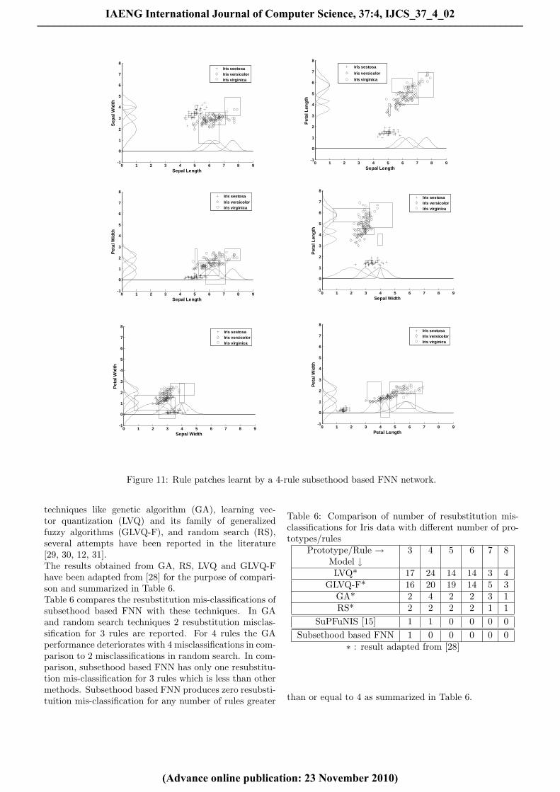
In classification problems, the purpose of the proposednetwork is to assign each pattern to one of a number ofclasses (or, more generally, to estimate the probabilityof membership of the case in each class). The Iris flowerdata set or Fisher’s Iris data set is a multivariate data setintroduced by Sir Ronald Aylmer Fisher as an exampleof discriminant analysis.

5.1 Iris data Classification

Iris data involves classification of three subspecies of theflower namely, Iris sestosa, iris versicolor and Iris vir-ginica on the basis of four feature measurements of theIris flower-sepal length, sepal width, petal length andpetal width [27]. There are 50 patterns (of four features)for each of the three subspecies of Iris flower. The in-put pattern set thus comprises 150 four-dimensional pat-terns. This data can be obtained from UCI repository ofmachine learning databases through the following link−http : //www.ics.uci.edu/ mlearn/MLRepository.html.The six possible scatter plots of Iris data are shown in Fig.10. It can be observed that classes Iris versicolor and Irisvirginica substantially overlap, while class Iris sestosa iswell separated from the other two. For this classificationproblem subsethood based FNN model employs a 4-r-3network architecture: the input layer consists of four nu-meric nodes; the output layer comprises three class nodes;and there are r rule nodes in the hidden layer.To train the network initially the centers of antecedentweight fuzzy sets were randomized in the range of theminimum and maximum values of respective input fea-tures of Iris data. Feature-wise, these ranges are (4.3,7.9), (2.0, 4.4), (1.0, 6.9) and (0.1, 2.5). The centers ofhidden-output weight fuzzy sets were randomized in the



______________________________________________________________________________________

4 4.5 5 5.5 6 6.5 7 7.5 82

2.5

3

3.5

4

4.5

5

Sepal Length

Sep

al W

idth

4 4.5 5 5.5 6 6.5 7 7.5 80

1

2

3

4

5

6

7

8

Sepal Length

Pet

al L

eng

th

Iris sestosaIris versicolorIris virginica

4 4.5 5 5.5 6 6.5 7 7.5 80

0.5

1

1.5

2

2.5

3

Sepal Length

Pet

al W

idth

2 2.5 3 3.5 4 4.50

1

2

3

4

5

6

7

8

Sepal WidthP

etal

Len

gth

2 2.5 3 3.5 4 4.50

0.5

1

1.5

2

2.5

3

Sepal Width

Pet

al W

idth

0 1 2 3 4 5 6 7 80

0.5

1

1.5

2

2.5

3

Petal Length

Pet

al W

idth

Figure 10: Six projection plots of Iris data.

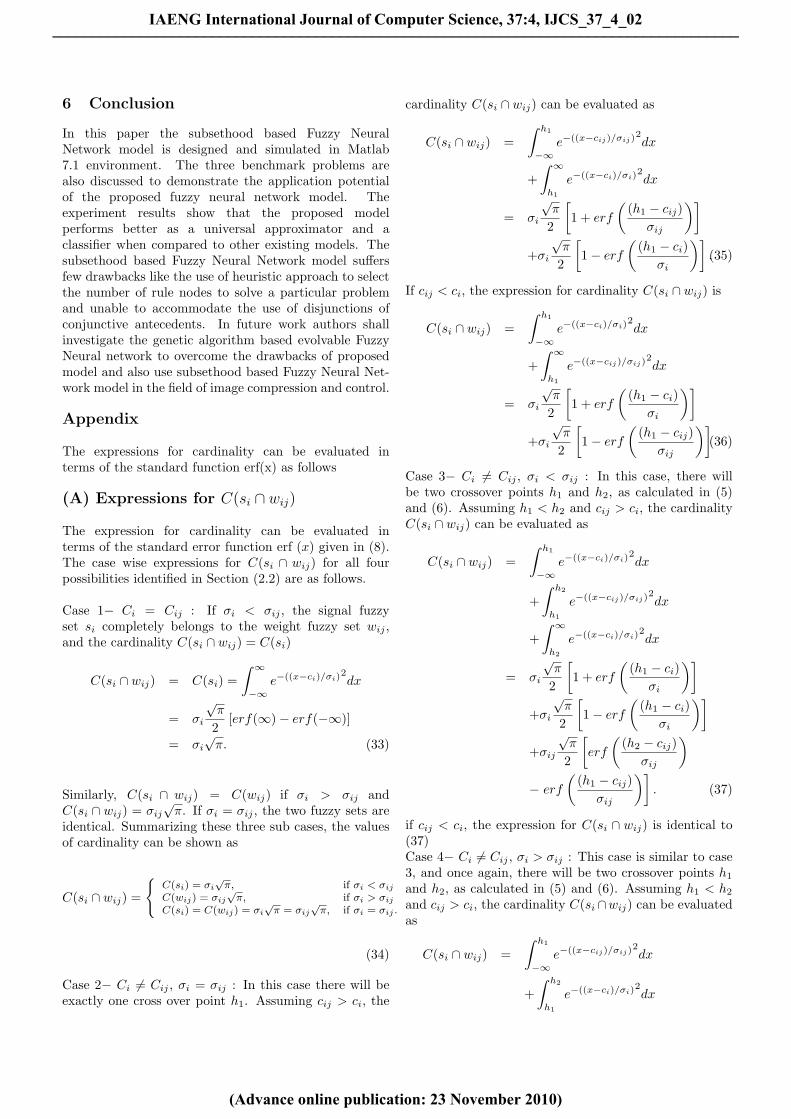
range (0,1) and the spreads of all fuzzy weights and fea-ture spreads were randomized in the range (0.2, 0.9). All150 patterns of the Iris data were presented sequentiallyto the input layer of the network for training. The learn-ing rate and momentum were kept constant at 0.001 dur-ing the training process. The test patterns which againcomprised all 150 patterns of Iris data were presentedto the trained network and the resubstitution error com-puted.Simulation experiments were conducted with differentnumbers of rule nodes to illustrate the performance ofthe classifier with a variation in the number of rules. No-tice that for r rules, the number of connections in the4-r-3 architecture for Iris data will be 7r. Because therepresentation of a fuzzy weight requires two parameters(center and spread), the total number of free parametersto be trained will be 14r+4.Table 5 summarizes the performance of proposed modelfor different rule counts. It is observed that except for rule

count 3 subsethood based FNIS model is able to achieve100 % resubstitution accuracy by classifying all patternscorrectly. Thus by merely using 60 parameters for subset-hood based FNN model produces no mis-classifications,and using only 46 free parameters 1 mis-classification isobtained. Apart from this, it is also observed from Table5 that as the numbers of rules increase the training rootmean square error (RMSE) decreases.As an example, the fuzzy weights of the trained networkwith four rules that produce zero resubstitution error areillustrated in the scatter plot of Iris data in Fig. 11. Therule patches in two dimensions were obtained by findingthe rectangular overlapping area produced by the projec-tion of 3σ points of the Gaussian fuzzy sets on differentinput feature axes of the same rule. The 3σ points werechosen because for 3σ on either side of centers of a Gaus-sian fuzzy set 99.7 % of the total area of the fuzzy setgets covered.To solve the Iris data classification problem using other



______________________________________________________________________________________

0 1 2 3 4 5 6 7 8 9-1

0

1

2

3

4

5

6

7

8

Sepal Length

Sep

al W

idth


0 1 2 3 4 5 6 7 8 9-1

0

1

2

3

4

5

6

7

8

Sepal Length

Pet

al L

eng

th

Iris sestosa

Iris versicolor

Iris virginica

0 1 2 3 4 5 6 7 8 9-1

0

1

2

3

4

5

6

7

8

Sepal Length

Pet

al W

idth


0 1 2 3 4 5 6 7 8 9-1

0

1

2

3

4

5

6

7

8

Sepal Width

Pet

al L

eng

th


0 1 2 3 4 5 6 7 8 9-1

0

1

2

3

4

5

6

7

8

Sepal Width

Pet

al W

idth


0 1 2 3 4 5 6 7 8 9-1

0

1

2

3

4

5

6

7

8

Petal Length

Pet

al W

idth


Figure 11: Rule patches learnt by a 4-rule subsethood based FNN network.

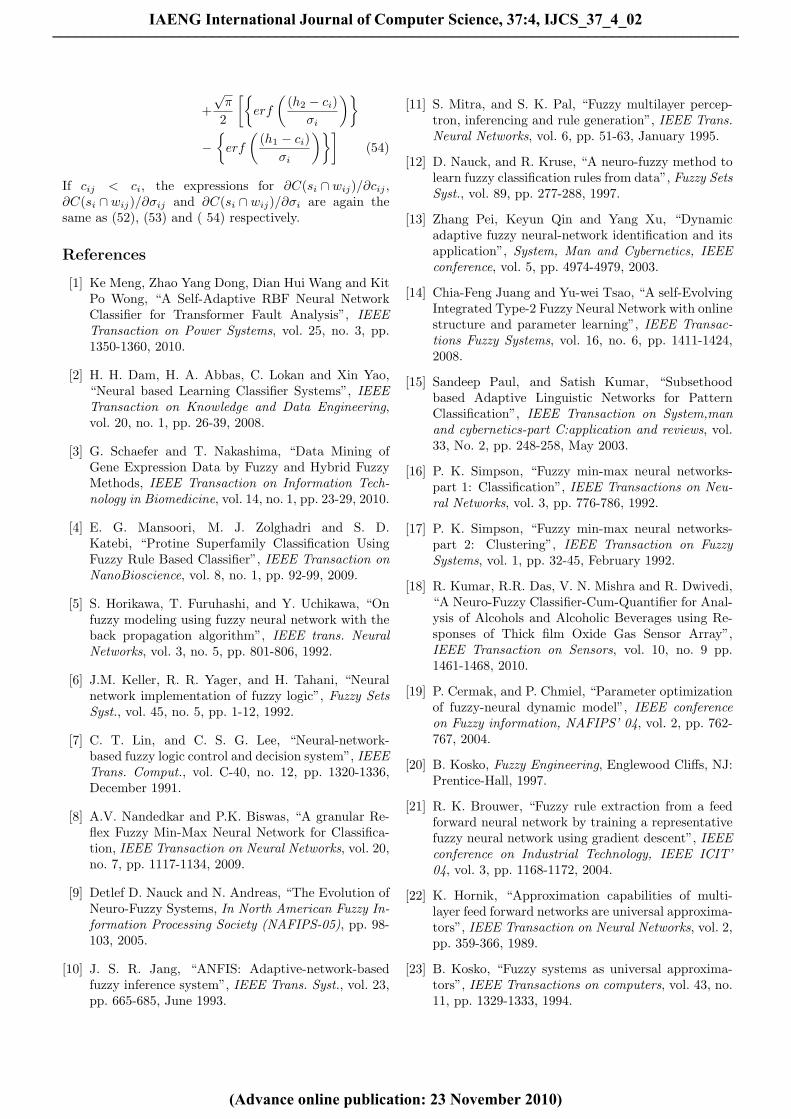
techniques like genetic algorithm (GA), learning vec-tor quantization (LVQ) and its family of generalizedfuzzy algorithms (GLVQ-F), and random search (RS),several attempts have been reported in the literature[29, 30, 12, 31].The results obtained from GA, RS, LVQ and GLVQ-Fhave been adapted from [28] for the purpose of compari-son and summarized in Table 6.Table 6 compares the resubstitution mis-classifications ofsubsethood based FNN with these techniques. In GAand random search techniques 2 resubstitution misclas-sification for 3 rules are reported. For 4 rules the GAperformance deteriorates with 4 misclassifications in com-parison to 2 misclassifications in random search. In com-parison, subsethood based FNN has only one resubstitu-tion mis-classification for 3 rules which is less than othermethods. Subsethood based FNN produces zero resubsti-tuition mis-classification for any number of rules greater

Table 6: Comparison of number of resubstitution mis-classifications for Iris data with different number of pro-totypes/rules

Prototype/Rule → 3 4 5 6 7 8Model ↓LVQ* 17 24 14 14 3 4

GLVQ-F* 16 20 19 14 5 3GA* 2 4 2 2 3 1RS* 2 2 2 2 1 1

SuPFuNIS [15] 1 1 0 0 0 0Subsethood based FNN 1 0 0 0 0 0

∗ : result adapted from [28]

than or equal to 4 as summarized in Table 6.



______________________________________________________________________________________

6 Conclusion

In this paper the subsethood based Fuzzy NeuralNetwork model is designed and simulated in Matlab7.1 environment. The three benchmark problems arealso discussed to demonstrate the application potentialof the proposed fuzzy neural network model. Theexperiment results show that the proposed modelperforms better as a universal approximator and aclassifier when compared to other existing models. Thesubsethood based Fuzzy Neural Network model suffersfew drawbacks like the use of heuristic approach to selectthe number of rule nodes to solve a particular problemand unable to accommodate the use of disjunctions ofconjunctive antecedents. In future work authors shallinvestigate the genetic algorithm based evolvable FuzzyNeural network to overcome the drawbacks of proposedmodel and also use subsethood based Fuzzy Neural Net-work model in the field of image compression and control.

Appendix

The expressions for cardinality can be evaluated interms of the standard function erf(x) as follows

(A) Expressions for C(si ∩ wij)

The expression for cardinality can be evaluated interms of the standard error function erf (x) given in (8).The case wise expressions for C(si ∩ wij) for all fourpossibilities identified in Section (2.2) are as follows.

Case 1− Ci = Cij : If σi < σij , the signal fuzzyset si completely belongs to the weight fuzzy set wij ,and the cardinality C(si ∩ wij) = C(si)

C(si ∩ wij) = C(si) =∫ ∞

−∞e−((x−ci)/σi)

2dx

= σi

√π

2[erf(∞)− erf(−∞)]

= σi

√π. (33)

Similarly, C(si ∩ wij) = C(wij) if σi > σij andC(si ∩ wij) = σij

√π. If σi = σij , the two fuzzy sets are

identical. Summarizing these three sub cases, the valuesof cardinality can be shown as

C(si ∩ wij) =

{C(si) = σi

√π, if σi < σij

C(wij) = σij√

π, if σi > σij

C(si) = C(wij) = σi√

π = σij√

π, if σi = σij .

(34)

Case 2− Ci 6= Cij , σi = σij : In this case there will beexactly one cross over point h1. Assuming cij > ci, the

cardinality C(si ∩ wij) can be evaluated as

C(si ∩ wij) =∫ h1

−∞e−((x−cij)/σij)

2dx

+∫ ∞

h1

e−((x−ci)/σi)2dx

= σi

√π

2

[1 + erf

((h1 − cij)

σij

)]

+σi

√π

2

[1− erf

((h1 − ci)

σi

)].(35)

If cij < ci, the expression for cardinality C(si ∩ wij) is



2dx

+∫ ∞

h1

e−((x−cij)/σij)2dx

= σi

√π

2

[1 + erf

((h1 − ci)

σi

)]

+σi

√π

2

[1− erf

((h1 − cij)

σij

)](36)

Case 3− Ci 6= Cij , σi < σij : In this case, there willbe two crossover points h1 and h2, as calculated in (5)and (6). Assuming h1 < h2 and cij > ci, the cardinalityC(si ∩ wij) can be evaluated as



2dx

+∫ h2

h1

e−((x−cij)/σij)2dx

+∫ ∞

h2


= σi

√π

2

[1 + erf

((h1 − ci)

σi

)]

+σi

√π

2

[1− erf

((h1 − ci)

σi

)]

+σij

√π

2

[erf

((h2 − cij)

σij

)

− erf

((h1 − cij)

σij

)]. (37)

if cij < ci, the expression for C(si ∩ wij) is identical to(37)Case 4− Ci 6= Cij , σi > σij : This case is similar to case3, and once again, there will be two crossover points h1

and h2, as calculated in (5) and (6). Assuming h1 < h2

and cij > ci, the cardinality C(si ∩wij) can be evaluatedas


−∞e−((x−cij)/σij)

2dx

+∫ h2

h1




______________________________________________________________________________________

+∫ ∞

h2

e−((x−cij)/σi)2dx

= σij

√π

2

[1 + erf

((h1 − cij)

σij

)]

+σij

√π

2

[1− erf

((h1 − cij)

σij

)]

+σi

√π

2

[erf

((h2 − ci)

σi

)

− erf

((h1 − ci)

σi

)]. (38)

If cij < ci the expression for cardinality is identical to(38).Corresponding expressions for E(si ∩ wij) are obtainedby substituting for C(si ∩ wij) from (34)-(38) in to (7).

(B) Expressions for ∂C(si ∩ wij)/∂cij,∂C(si ∩ wij)/∂σij and ∂C(si ∩ wij)/∂σi

As per the discussion in the Section (3.2) that, thecalculation of ∂C(si ∩ wij)/∂cij , ∂C(si ∩ wij)/∂σij and∂C(si ∩ wij)/∂σi is required in (23), (24) and (25) whichdepends on the nature of overlap. Therefore the casewise expressions are given as following:

Case 1− Ci = Cij : As is evident from (34), C(si ∩ wij)is independent of cij , and therefore,

∂C(si ∩ wij)∂cij

= 0. (39)

similarly the first derivative of (34) with respect to σij

and σi is,

∂C(si ∩ wij)∂σij

={ √

π, if cij = ci and σij ≤ σi

0, if cij = ci and σij > σi.(40)

∂C(si ∩ wij)∂σi

={

0, if cij = ci and σij < σi√π, if cij = ci and σij ≥ σi.

(41)

Case 2− Ci 6= Cij , σi = σij : Whencij > ci, ∂C(si ∩ wij)/∂cij , ∂C(si ∩ wij)/∂σij and∂C(si ∩ wij)/∂σi are derived by differentiating (35) asfollows :


=∫ h1

−∞

∂

∂cije−((x−cij)/σij)

2dx

+∫ ∞

h1

∂

∂cije−((x−ci)/σi)

2dx

=∫ h1

−∞

∂


2dx

= −e−((h1−cij)/σij)2

(42)


=∫ h1

−∞

∂

∂σije−((x−cij)/σij)

2dx

+∫ ∞

h1

∂

∂σije−((x−ci)/σi)

2dx

= −h1 − cij

σije−((h1−cij)/σij)

2

+√

π

2

[erf

((h1 − cij)

σij

)+ 1

](43)


=∫ h1

−∞

∂

∂σie−((x−cij)/σij)

2dx

+∫ ∞

h1

∂

∂σie−((x−ci)/σi)

2dx

=h1 − ci

σie−((h1−ci)/σi)

2

−√

π

2

[erf

((h1 − ci)

σi

)− 1

](44)

When cij < ci, ∂C(si ∩ wij)/∂cij , ∂C(si ∩ wij)/∂σij and∂C(si ∩ wij)/∂σi are derived by differentiating (36) asfollows :


=∫ h1

−∞

∂


2dx

+∫ ∞

h1

∂


2dx

=∫ ∞

h1

∂


2dx

= e−((h1−cij)/σij)2

(45)


=∫ h1

−∞

∂


2dx

+∫ ∞

h1

∂


2dx

= −h1 − cij


2

−√

π

2

[erf

((h1 − cij)

σij

)− 1

](46)


=∫ h1

−∞

∂


2dx

+∫ ∞

h1

∂


2dx

= −h1 − ci


2

+√

π

2

[erf

((h1 − ci)

σi

)+ 1

](47)

Case 3− Ci 6= Cij , σi < σij : Once again, twosub cases arise similar to those of Case 2. Whencij > ci, ∂C(si ∩ wij)/∂cij , ∂C(si ∩ wij)/∂σij and∂C(si ∩ wij)/∂σi are derived by differentiating (37).


=∫ h1

−∞

∂


2dx



______________________________________________________________________________________

+∫ h2

h1

∂


2dx

+∫ ∞

h2

∂


2dx

=∫ h2

h1

∂


2dx


+e−((h1−cij)/σij)2

(48)


=∫ h1

−∞

∂


2dx

+∫ h2

h1

∂


2dx

+∫ ∞

h2

∂


2dx

=∫ h2

h1

∂


2dx

=h1 − cij


2

−h2 − cij


2

+√

π

2

[−erf

((h1 − cij)

σij

)

+ erf

((h2 − cij)

σij

)](49)


=∫ h1

−∞

∂


2dx

+∫ h2

h1

∂


2dx

+∫ ∞

h2

∂


2dx

=∫ h1

−∞

∂


2dx

+∫ ∞

h2

∂


2dx

= −h1 − ci


2

+h2 − ci


2

+√

π

2

[{erf

((h1 − ci)

σi

)+ 1

}

−{

erf

((h2 − cij)

σij

)− 1

}](50)

Similarly, if cij < ci


=∫ h1

−∞

∂


2dx

+∫ h2

h1

∂


2dx

+∫ ∞

h2

∂


2dx

=∫ h2

h1

∂


2dx



(51)

Thus for both the cases (cij < ci or cij > ci),identical expressions for ∂C(si ∩ wij)/∂cij are obtained.Similarly, the expressions for ∂C(si ∩ wij)/∂σij and∂C(si ∩ wij)/∂σi also remain the same as (49) and (50)respectively in both the conditions.Case 4− Ci 6= Cij , σi > σij : Whencij > ci, ∂C(si ∩ wij)/∂cij , ∂C(si ∩ wij)/∂σij and∂C(si ∩ wij)/∂σi are derived by differentiating (38) as


=∫ h1

−∞

∂


2dx

+∫ h2

h1

∂


2dx



(52)


=∫ h1

−∞

∂


2dx

+∫ h2

h1

∂


2dx

+∫ ∞

h2

∂


2dx

=h1 − cij


2

−h2 − cij


2

+√

π

2

[2 + erf

((h1 − cij)

σij

)

− erf

((h2 − cij)

σij

)](53)


=∫ h1

−∞

∂


2dx

+∫ h2

h1

∂


2dx

+∫ ∞

h2

∂


2dx

=h1 − ci


2

−h2 − ci


2



______________________________________________________________________________________

+√

π

2

[{erf

((h2 − ci)

σi

)}

−{

erf

((h1 − ci)

σi

)}](54)

If cij < ci, the expressions for ∂C(si ∩ wij)/∂cij ,∂C(si ∩ wij)/∂σij and ∂C(si ∩ wij)/∂σi are again thesame as (52), (53) and ( 54) respectively.

References

[1] Ke Meng, Zhao Yang Dong, Dian Hui Wang and KitPo Wong, “A Self-Adaptive RBF Neural NetworkClassifier for Transformer Fault Analysis”, IEEETransaction on Power Systems, vol. 25, no. 3, pp.1350-1360, 2010.

[2] H. H. Dam, H. A. Abbas, C. Lokan and Xin Yao,“Neural based Learning Classifier Systems”, IEEETransaction on Knowledge and Data Engineering,vol. 20, no. 1, pp. 26-39, 2008.

[3] G. Schaefer and T. Nakashima, “Data Mining ofGene Expression Data by Fuzzy and Hybrid FuzzyMethods, IEEE Transaction on Information Tech-nology in Biomedicine, vol. 14, no. 1, pp. 23-29, 2010.

[4] E. G. Mansoori, M. J. Zolghadri and S. D.Katebi, “Protine Superfamily Classification UsingFuzzy Rule Based Classifier”, IEEE Transaction onNanoBioscience, vol. 8, no. 1, pp. 92-99, 2009.

[5] S. Horikawa, T. Furuhashi, and Y. Uchikawa, “Onfuzzy modeling using fuzzy neural network with theback propagation algorithm”, IEEE trans. NeuralNetworks, vol. 3, no. 5, pp. 801-806, 1992.

[6] J.M. Keller, R. R. Yager, and H. Tahani, “Neuralnetwork implementation of fuzzy logic”, Fuzzy SetsSyst., vol. 45, no. 5, pp. 1-12, 1992.

[7] C. T. Lin, and C. S. G. Lee, “Neural-network-based fuzzy logic control and decision system”, IEEETrans. Comput., vol. C-40, no. 12, pp. 1320-1336,December 1991.

[8] A.V. Nandedkar and P.K. Biswas, “A granular Re-flex Fuzzy Min-Max Neural Network for Classifica-tion, IEEE Transaction on Neural Networks, vol. 20,no. 7, pp. 1117-1134, 2009.

[9] Detlef D. Nauck and N. Andreas, “The Evolution ofNeuro-Fuzzy Systems, In North American Fuzzy In-formation Processing Society (NAFIPS-05), pp. 98-103, 2005.

[10] J. S. R. Jang, “ANFIS: Adaptive-network-basedfuzzy inference system”, IEEE Trans. Syst., vol. 23,pp. 665-685, June 1993.

[11] S. Mitra, and S. K. Pal, “Fuzzy multilayer percep-tron, inferencing and rule generation”, IEEE Trans.Neural Networks, vol. 6, pp. 51-63, January 1995.

[12] D. Nauck, and R. Kruse, “A neuro-fuzzy method tolearn fuzzy classification rules from data”, Fuzzy SetsSyst., vol. 89, pp. 277-288, 1997.

[13] Zhang Pei, Keyun Qin and Yang Xu, “Dynamicadaptive fuzzy neural-network identification and itsapplication”, System, Man and Cybernetics, IEEEconference, vol. 5, pp. 4974-4979, 2003.

[14] Chia-Feng Juang and Yu-wei Tsao, “A self-EvolvingIntegrated Type-2 Fuzzy Neural Network with onlinestructure and parameter learning”, IEEE Transac-tions Fuzzy Systems, vol. 16, no. 6, pp. 1411-1424,2008.

[15] Sandeep Paul, and Satish Kumar, “Subsethoodbased Adaptive Linguistic Networks for PatternClassification”, IEEE Transaction on System,manand cybernetics-part C:application and reviews, vol.33, No. 2, pp. 248-258, May 2003.

[16] P. K. Simpson, “Fuzzy min-max neural networks-part 1: Classification”, IEEE Transactions on Neu-ral Networks, vol. 3, pp. 776-786, 1992.

[17] P. K. Simpson, “Fuzzy min-max neural networks-part 2: Clustering”, IEEE Transaction on FuzzySystems, vol. 1, pp. 32-45, February 1992.

[18] R. Kumar, R.R. Das, V. N. Mishra and R. Dwivedi,“A Neuro-Fuzzy Classifier-Cum-Quantifier for Anal-ysis of Alcohols and Alcoholic Beverages using Re-sponses of Thick film Oxide Gas Sensor Array”,IEEE Transaction on Sensors, vol. 10, no. 9 pp.1461-1468, 2010.

[19] P. Cermak, and P. Chmiel, “Parameter optimizationof fuzzy-neural dynamic model”, IEEE conferenceon Fuzzy information, NAFIPS’ 04, vol. 2, pp. 762-767, 2004.

[20] B. Kosko, Fuzzy Engineering, Englewood Cliffs, NJ:Prentice-Hall, 1997.

[21] R. K. Brouwer, “Fuzzy rule extraction from a feedforward neural network by training a representativefuzzy neural network using gradient descent”, IEEEconference on Industrial Technology, IEEE ICIT’04, vol. 3, pp. 1168-1172, 2004.

[22] K. Hornik, “Approximation capabilities of multi-layer feed forward networks are universal approxima-tors”, IEEE Transaction on Neural Networks, vol. 2,pp. 359-366, 1989.

[23] B. Kosko, “Fuzzy systems as universal approxima-tors”, IEEE Transactions on computers, vol. 43, no.11, pp. 1329-1333, 1994.



______________________________________________________________________________________

[24] C. T. Lin, and Y. C. Lu, “A neural fuzzy systemwith linguistic teaching signals”, IEEE TransactionsFuzzy Systems, vol. 3, no. 2, pp. 169-189, 1995.

[25] L. X. Wang, and J. M.Mendel, “Generating fuzzyrules from numerical data, with application”, Tech.Rep. 169, USC SIPI, Univ. Southern California, LosAngeles, January 1991.

[26] H. Narazaki, and A. L. Ralescu, “An improved syn-thesis method for multilayered neural networks usingqualitative knowledges”, IEEE Transactions FuzzySystems, vol. 1, no. 2, pp. 125-137, 1993.

[27] R. A. Fisher, “The use of multiple measurements intaxonomic problems.”, Ann. Eugenics, 7, 2, 179-188,1986.

[28] L. I. Kuncheva, and J. C. Bezdek, “Nearest proto-type classification: Clustering, genetic algorithms orrandom search?”, IEEE Trans. Syst., Man, Cybern.,vol. C 28, pp.160-164, February 1998.

[29] S. Halgamuge and M.Glesner, “Neural networks indesigning fuzzy systems for real world applications”,Fuzzy Sets Syst., vol. 65, pp. 1-12, 1994.

[30] N. Kasabov, and B. Woodford, “Rule insertion andrule extraction from evolving fuzzy neural networks:Algorithms and applications for building adaptive,intelligent expert systems”, In Proc. IEEE Intl.Conf. Fuzzy Syst. FUZZ-IEEE 99, Seoul, Korea, vol.3, pp. 1406-1411, August 1999.

[31] M. Russo, “FuGeNeSys-a fuzzy genetic neural sys-tem for fuzzy modeling”, IEEE Transactions FuzzySystems, vol. 6, no. 3, pp. 373-388, 1993.

[32] Y. Lin, and G. A. Cunningham III, “A new approachto fuzzy-neural system modeling”, IEEE Transac-tions Fuzzy Systems, vol. 3, no. 2, pp. 190-198, 1995.



______________________________________________________________________________________

design of fuzzy neural network for function approximation ... · pdf filedesign of fuzzy...

Documents