design of experimentansytech.com/doe-day7.pdf · · 2008-02-08§2k factorial with center point...
TRANSCRIPT

© AnsyTech 2008
Design of Experiment
ANSY Tech. Inc.Muhammad Sohail Ahmed, Ph.D.Mubashir Siddiqui

© AnsyTech 2008
Day 7
Factorial Design – 3 Levels

© AnsyTech 2008
Factorial Designs (Day 7)
§ 2k Factorial with Center Point§ 32 Factorial Design§ 33 Factorial Design§ Confounding

© AnsyTech 2008
Methods to Obtain Curvature Estimate
§ 2k design with center points
§ 3-Level Designs
§ Response Surface Method

© AnsyTech 2008
2k Factorial with Center Pointεβββ +++= ∑∑∑
<= jijiij
k
jjj xxx
10 y First Order Model
To model CURVATURE in Response Function
εββββ ++++= ∑∑∑∑<== ji
jiij
k
jjjj
k
jjj xxxx
1
2
10 y
where ßjj: pure second order or quadratic effects
(1) a
b ab
A-B- A+B-
A+B+A-B+
Low High
Low
HighB
A
Let nc be the observations at center point (0,0)Let yF be the observations at corner points (0,0).

© AnsyTech 2008
Problem
Response: Yield of a chemical processFactors: Reaction Time and
Reaction Temperature
(a) Find significant factors, their effects.(b) Is there any evidence of curvature?

© AnsyTech 2008
Entering Data in Minitab

© AnsyTech 2008
Solution
Stat à DOE à Define Custom Factorial Design

© AnsyTech 2008
Solution (cont’d)
Stat à DOE à Analyze Factorial Design

© AnsyTech 2008
Solution (cont’d)
No evidence of second order curvature for the region tested

© AnsyTech 2008
32 Design
Low level Intermediate Level High Level

© AnsyTech 2008
32 Design Model
Low level Intermediate Level High Level
Notice the quadratic nature of the model

© AnsyTech 2008
ProblemAn experiment is run in a chemical process using a 32 factorial design. The design factors
are temperature and pressure, and the response variable is yield. Data is shown in the table.
(a) Using ANOVA, which factor has significant effects?
(b) Analyze the residuals.
(c) Verify that the second order model could be written, in natural variables, as
y = -1335.63 + 18.56T + 8.59P – 0.072T2 – 0.0196P2 – 0.0384TP(d) Verify that if we let low, medium, and high levels be represented by -1, 0, and
+1, then the second order model for yield isy = 86.81 + 10.4x1 + 8.42x2 – 7.17x1
2 – 7.86x22 – 7.69x1x2
76.58, 83.0496.57, 88.7271.18, 92.77100
93.95, 88.5488.47, 84.2351.86, 82.4390
80.92, 72.6064.97, 69.2247.58, 48.7780
140120100
Pressure (psig)Temperature
0C

© AnsyTech 2008
Solution
83.04100140
88.5490140
72.680140
88.72100120
84.2390120
69.2280120
92.77100100
82.4390100
48.7780100
76.58100140
93.9590140
80.9280140
96.57100120
88.4790120
64.9780120
71.18100100
51.8690100
47.5880100
YTP
Entering Data in Minitab

© AnsyTech 2008
Solution
Solution (a) Using ANOVA, which factors are significant?Stat à ANOVA à Two-WaySelect Y as response and Pressure and Temperature as Factors.Click on Graphs, Select Four in One for Residual Plots.
Pressure and Temperature are significant. Their interaction is not.

© AnsyTech 2008
Solution (cont’d)Solution (b) Analyze residuals.We will get residuals plot by selecting Four in One for Residual Plots.
20100-10-20
99
90
50
10
1
Residual
Per
cent
9080706050
10
0
-10
Fitted Value
Res
idua
l
151050-5-10-15
6.0
4.5
3.0
1.5
0.0
Residual
Freq
uenc
y
18161412108642
10
0
-10
Observation Order
Res
idua
l
Normal Probability Plot Versus Fits
Histogram Versus Order
Residual Plots for Y
Residuals seem to be normally distributed in Normal Probability Plot.But the plot of residuals vs fits shows a converging nozzle. Hence there is non-constant variance.

© AnsyTech 2008
Residuals VS Fitted Values
n As the magnitude of observation increases, the variance increases.
n Error in measuring instrument.n Data follows a non-normal or skewed
distribution.n F-test is only slightly affected in balanced
designs.n In worse cases, data transformation is required.
§

© AnsyTech 2008
Solution (cont’d)Solution (c)Verify that the second order model could be written, in natural variables, as
y = -1335.63 + 18.56T + 8.59P – 0.072T2 – 0.0196P2 – 0.0384TP

© AnsyTech 2008
Solution (cont’d)
Stat à Regression à RegressionSelect Response and Predictors.
© AnsyTech 2008
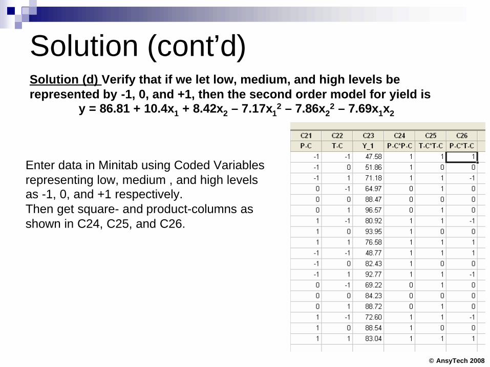
Solution (cont’d)Solution (d) Verify that if we let low, medium, and high levels be represented by -1, 0, and +1, then the second order model for yield is
y = 86.81 + 10.4x1 + 8.42x2 – 7.17x12 – 7.86x2
2 – 7.69x1x2
Enter data in Minitab using Coded Variablesrepresenting low, medium , and high levels as -1, 0, and +1 respectively.Then get square- and product-columns as shown in C24, C25, and C26.

© AnsyTech 2008
Solution (cont’d)Stat à Regression à RegressionSelect Response and Predictors.

© AnsyTech 2008
3-D view Of Response y=f(T,P)
h t tp : / /www. l i vephys ics .com/p too ls /on l i ne - 3 d-f u n c t i o n - grapher.php?ymin=- 1 & x m i n = - 1 & z m i n = A u t o & y m a x = 1 & x m a x = 1 & z m a x =Auto&f =86.81%2B%2810.4*x%29%2B%288.42*y%29 -% 2 8 7 . 1 * x % 5 E 2 % 2 9 -%287.86*y%5E2%29 -% 2 8 7 . 6 9 * x * y % 2 9

© AnsyTech 2008
Same Problem Using Factorial Design
Stat à DOE à Define Custom Factorial Design

© AnsyTech 2008
Same Problem Using Factorial DesignStat à DOE à Analyze Factorial DesignSelect Response

© AnsyTech 2008
33 Design

© AnsyTech 2008
33 DesignThree factors are being studied viz bottle type, shelf type, and workers to find theireffects on the time it takes to stock 10 cases on shelves. Time data is as shown here.(a) Which of the factors are significant?(b) Specify appropriate levels of factors..

© AnsyTech 2008
Entering Data in Minitab

© AnsyTech 2008
SolutionSolution (a) – Significant FactorsStat à DOE à Define Custom Factorial DesignSelect Factors.Check ‘General Factorial Design’

© AnsyTech 2008
Solution (cont’d)Stat à DOE à Analyze Factorial DesignSelect Response.Click Graphs. Select Four In One under Residuals Plot.

© AnsyTech 2008
Solution (cont’d)
0.500.250.00-0.25-0.50
99
90
50
10
1
Residual
Pe
rce
nt
6543
0.4
0.2
0.0
-0.2
-0.4
Fitted Value
Re
sid
ua
l
0.320.160.00-0.16-0.32
8
6
4
2
0
Residual
Fre
qu
ency
50454035302520151051
0.4
0.2
0.0
-0.2
-0.4
Observation Order
Re
sid
ua
l
Normal Probability Plot Versus Fits
Histogram Versus Order
Residual Plots for Time

© AnsyTech 2008
Solution (cont’d)
321
5.6
5.2
4.8
4.4
4.0321
321
5.6
5.2
4.8
4.4
4.0
Worker
Me
an
Bottle Type
Shelf Type
Main Effects Plot for TimeData Means
Solution (b)Stat à DOE à Factorial Plots

© AnsyTech 2008
Solution (cont’d)
321 321
6
5
4
6
5
4
Wor ker
Bottle T ype
Shelf T ype
123
Worker
123
TypeBottle
Interaction Plot for TimeData Means
Shortest Time:Worker: 1 (or 3)Shelf Type:1

© AnsyTech 2008
Confounding
© AnsyTech 2008
Confounding
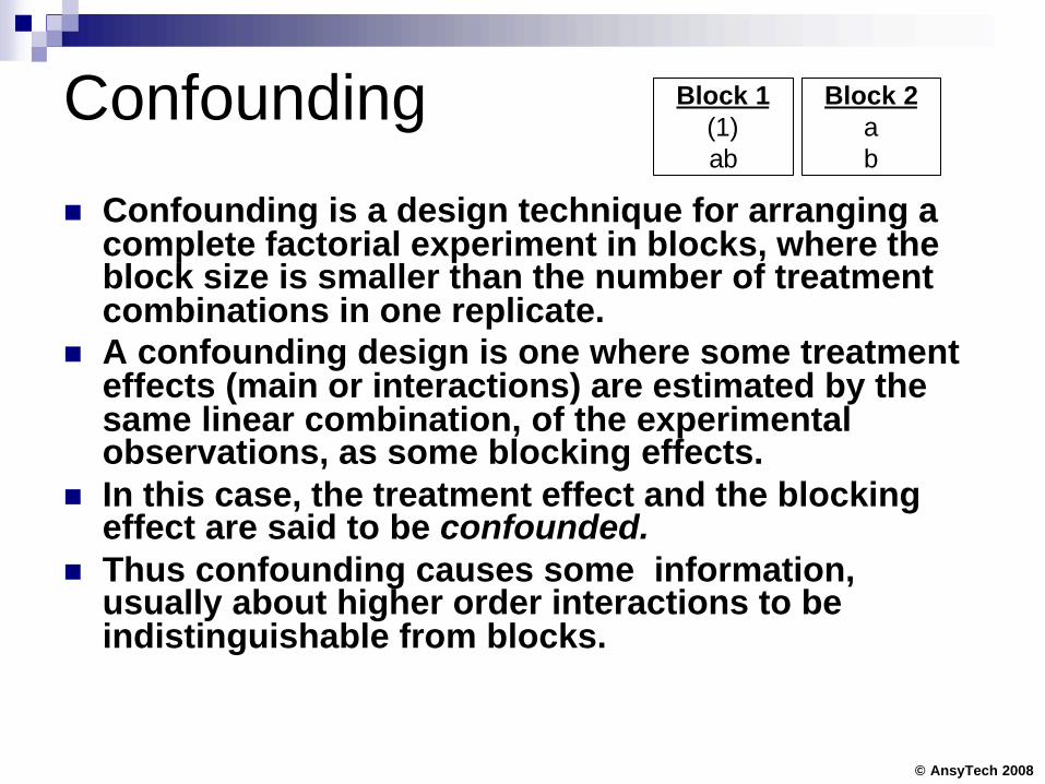
n Confounding is a design technique for arranging a complete factorial experiment in blocks, where the block size is smaller than the number of treatment combinations in one replicate.
n A confounding design is one where some treatment effects (main or interactions) are estimated by the same linear combination, of the experimental observations, as some blocking effects.
n In this case, the treatment effect and the blocking effect are said to be confounded.
n Thus confounding causes some information, usually about higher order interactions to be indistinguishable from blocks.
Block 1(1)ab
Block 2ab

© AnsyTech 2008
Confounding
ab++4
b+-3
a-+2
(1)--1
CombinationBARuns
Block 1(1)ab
Block 2ab
Assignment of four runs of a 22 Design in Two BLOCKS
])1([
])1([
])1([
21
21
21
baabABEffectnInteractio
abbaBBofeffectMain
abbaAAofeffectMain
n
n
n
−−+==
++−−==
+−+−==
Which effects are confounded?See the SIGNS in Main and Interaction Effects. Here AB effect is confounded.

© AnsyTech 2008
ProblemFour factors are studied to find their effects on Filtration Rate. They are:Temperature(A), Pressure(B), Concentration of formaldehyde(C), and Stirring Rate(D).All combinations cannot be run using one batch of raw materials.So there will be two blocks.
Block 1(1)=25ab=45ac=40bc=60ad=80bd=25cd=55
abcd=76
Block 2a=71b=48c=68d=43
abc=65bcd=70acd=86
abd=104
1
1
1
1
1
1
1
1
-1
-1
-1
-1
-1
-1
-1
-1
D
abcd
bcd
acd
cd
abd
bd
ad
d
abc
bc
ac
c
ab
b
a
(1)
Comb
111
11-1
1-11
1-1-1
-111
-11-1
-1-11
-1-1-1
111
11-1
1-11
1-1-1
-111
-11-1
-1-11
-1-1-1
CBA
ABCD = + ABCD = -

© AnsyTech 2008
Entering Data in Minitab
© AnsyTech 2008
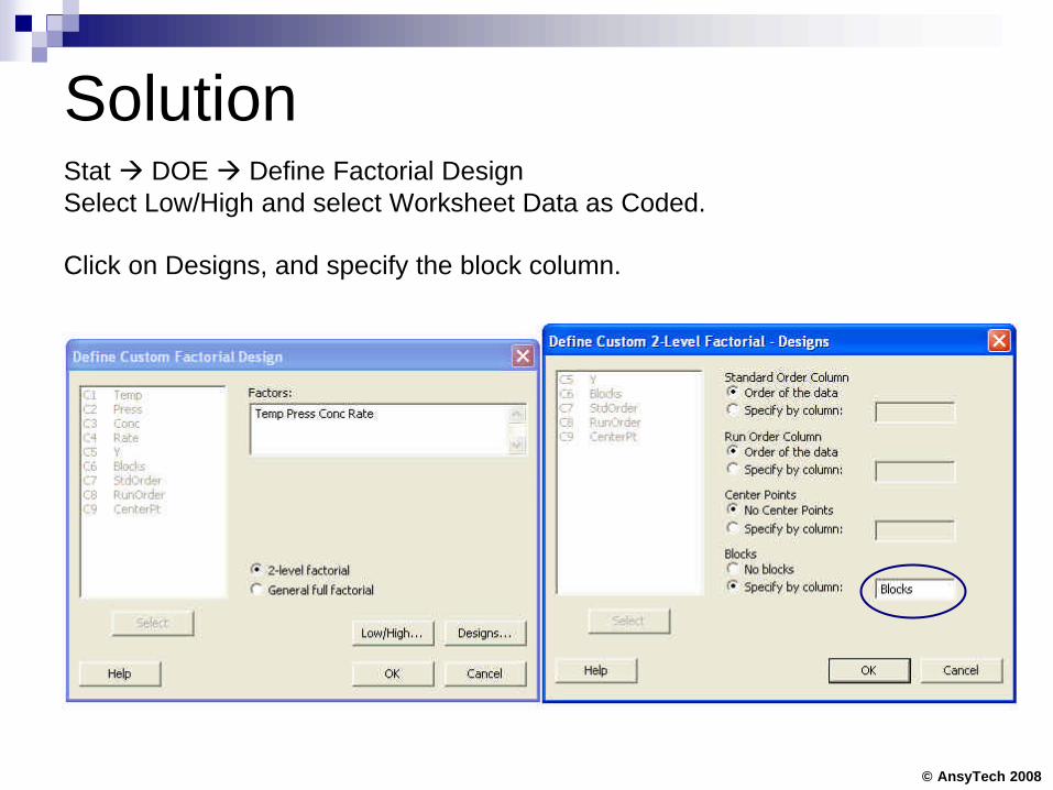
SolutionStat à DOE à Define Factorial DesignSelect Low/High and select Worksheet Data as Coded.
Click on Designs, and specify the block column.

© AnsyTech 2008
Solution (cont’d)

© AnsyTech 2008
Solution (cont’d)
20100-10-20
99
95
90
80
7060504030
20
10
5
1
Effect
Per
cen
t
A TempB PressC ConcD Rate
Factor Name
Not SignificantSignificant
Effect Type
AD
AC
DC
A
Normal Plot of the Effects(response is Y, Alpha = .05)
Lenth's PSE = 3.1875

© AnsyTech 2008
End of Day 7