Design of Beam Lines and KEK Beam Lines

Akihiro Maki

KEK

141 ­

Design of Beam Lines and KEK Beam Lines

1. Introduction

The gross characteristics of the experimental beams are limitted by the maximum energy and intensity of

the accelerator where the beams are installed.' The parameters of our synchrotron (KEK -PS). that is,

maximum energy of 8 to 12 GeV. beam intensity of 1012 to 1013 ppp and so on, Eletermine the production

rates of secondary particles. So the beam design is how to gather these particles effectively. how to separate

specific particles, how to focus and so on.

The experimental beams which I would present today are not the finally authoriz~ plans, but plans which

are now on the process of more detailed consideration. Since the budget is very severe, all the required

beams are not installed at the early stage. It depends very much on the physics what kind of beams must

be installed here at first I would like to recomend here that they will be reconsidered according to future

discussions on physics.

Today I will give you, at first. a short review of beam optics and will introduce you some kinds of beam line

elements which are now under construction at our laboratory. Next, I will give you some examples of beam

design, and I will enclose some important problems which we encounter in the work of beam design.

-143 ­

II Beam Design

II -1 Beam Optics

Now, let us confine ourselves to handle only charged particles for a time. Usually we handle them with

electric and magnetic field of special configuration. So the motion of each particle is completely described by

the familiar Lorentz equation:

d(IT(m V) =e (E + V XE) (2.1)

According to this equation, it is clear that a magnetic field of 10 KG gives the same force as a electric field of

3 X 10 6 V fcm to a particle traveling with the light velocity. The practical limit of today's industrial technique

for magnetic field produced by ordinary iron magnet and for electric field are, respectively, about 20 KG

and 10 5 V fcm. This is the reason why we use magnetic devices in most cases of beam handling. Of course,

electric ones are also used in special cases as will be described in the following.

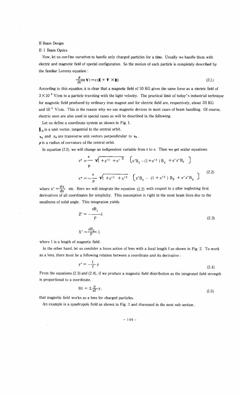
Let us define a coordinate system as shown in Fig. 1.

$0 is a unit vector, tangential to the central orbit.

Xo and Yo are transverse unit vectors perpendicular to So •

p is a radius of curvature of the central orbit.

In equation (2.1). we will change an indipendent variable from t to s. Then we get scalar equations

Z~ =-=-- vi + Z'2 +x' 2 (x'B - (1 +z' 2 ) Bx + x' z' Bz Js p

(2.2)

x~ =-=.:~ vi +Z'2 + X' 2 (z'Bs (1 +X'2) Bz +x'z'B x J p

where x' = ~:, . etc. Here we will integrate the equation (2.2) with respect to s after neglecting first

derivatives of all coordinates for simplicity. This assumption is right in the most beam lines due to the

smallness of solid angle. This integration yields

eB x

Z' = ---1 p (2.3)

X' = eBz 1 p

where 1 is a length of magnetic field.

In the other hand. let us condider a focus action of lens with a focal length f as shown in Fig. 2. To work

as a lens, there must be a following relation between a coordinate and its derivative:

, 1 y = --f- y

(2.4)

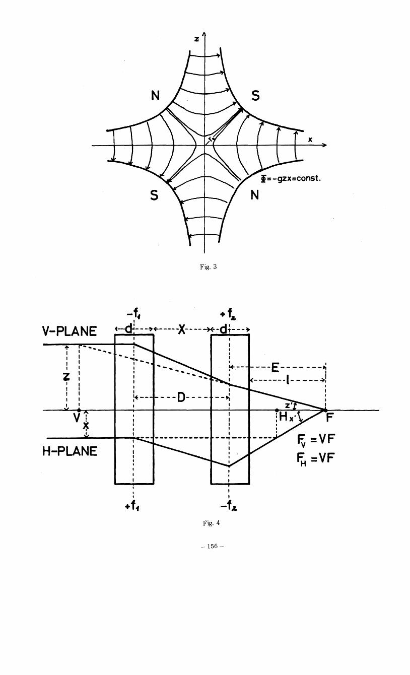
From the equations (2.3) and (2.4), if we produce a magnetic field distribution as the integrated field strength

is proportional to a coordinate.

Bl = + p y~er ' (1.5)

that magnetic field works as a lens for charged particles.

An example is a quadrupole field as shown in Fig. 3 and discussed in the next sub-section.

-144 ­

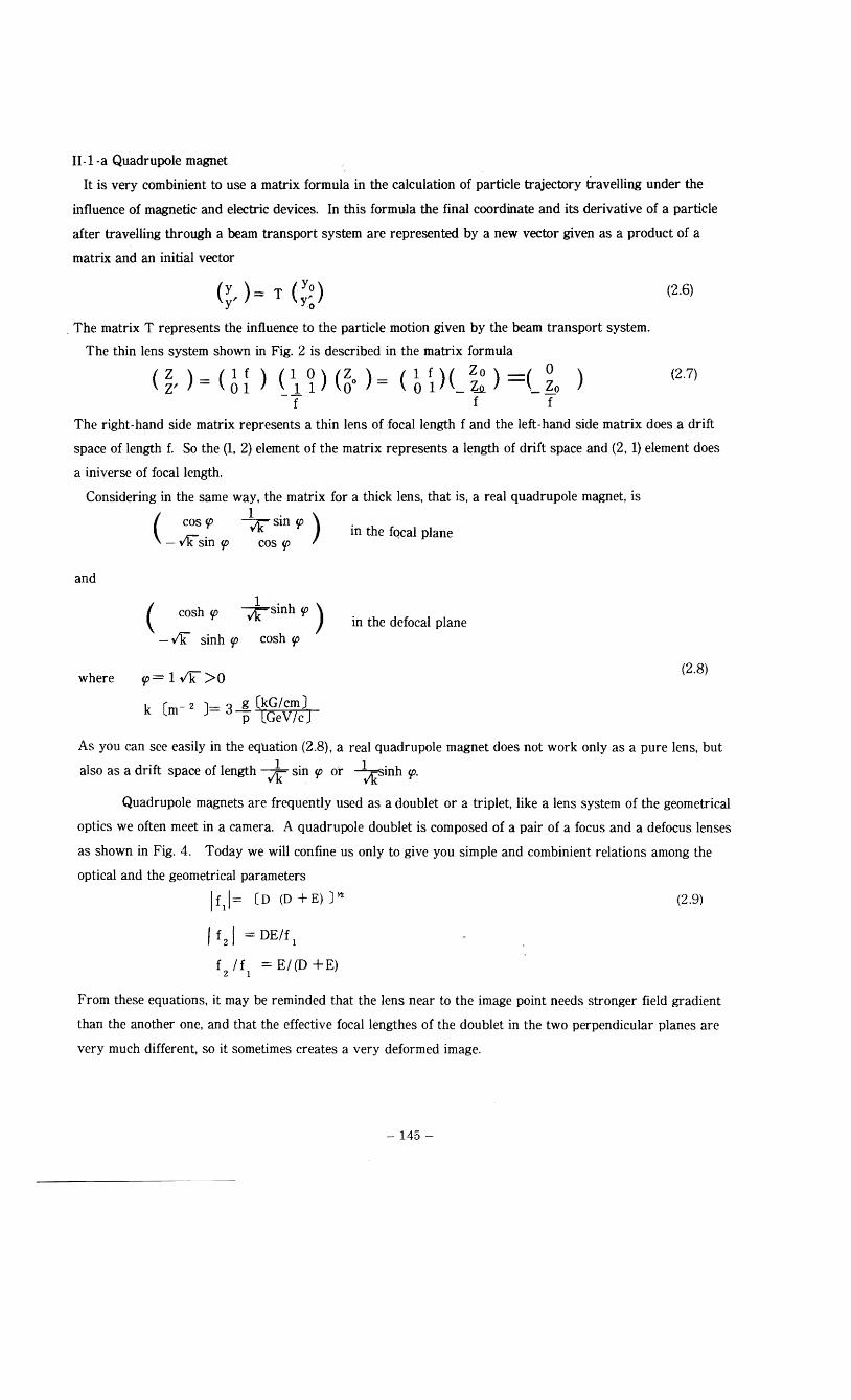
1I-1-a Quadrupole magnet

It is very combinient to use a matrix formula in the calculation of particle trajectory travelling under the

influence of magnetic and electric devices. ,In this formula the final coordinate and its derivative of a particle

after travelling through a beam transport system are represented by a new vector given as a product of a

matrix and an initial vector

(Y,)= T (yY2) (2.6) Yo

. The matrix T represents the influence to the particle motion given by the beam transport system.

The thin lens system shown in Fig. 2 is described in the matrix formula

(2.7)( ~, ) = ( 6r ) (\~) (~o ) = (t i) (_ ~ )=(_ ~o ) -T f f

The right-hand side matrix represents a thin lens of focal length f and the left-hand side matrix does a drift

space of length f. So the (1, 2) element of the matrix represents a length of drift space and (2, 1) element does

a iniverse of focal length.

Considering in the same way, the matrix for a thick lens, that is, a real quadrupole magnet, is

1.)cos tp ~sm tp( in the fQcal plane¥ksin tp cos <p

and

( cosh'P *Sinh'P) in the defocal plane - v'k sinh tp cosh tp

(2.8)where tp= llk>O

3 g (kG/cm) p (GeV/c)

As you can see easily in the equation (2.8), a real quadrupole magnet does not work only as a pure lens, but

also as a drift space of length Jz sin tp o'r ~inh tp.

Quadrupole magnets are frequently used as a doublet or a triplet, like a lens system of the geometrical

optics we often meet in a camera. A quadrupole doublet is composed of a pair of a focus and a defocus lenses

as shown in Fig. 4. Today we will confine us only to give you simple and combinient relations among the

optical and the geometrical parameters

If 11 = [0 (0 + E) JYl (2.9)

I f2/ = DElf 1

f If = E/(D +E)2 1

From these equations, it may be reminded that the lens near to the image point needs stronger field gradient

than the another one, and that the effective focal lengthes of the doublet in the two perpendicular planes are

very much different, so it sometimes creates a very deformed image.

- 145

To overcome this defect of the doublet, a triplet is sometimes used. But triplet has other defect comparing

with the doublet. Triplet requires a larger g. 1 value and a larger cost for the same effective focal length and

the same beam momentum.

II-1-b Bending Magnet

The bending magnets used as a beam line elements, in most cases, satisfy the symmetry equations

By (Y)=By (-y) Bx(y)= Bx (-y) Bs(Y)= Bs(-y) (2.10)

Then the equations of motion are obtained in the linear approximation

z~ + kz = 0

(2.11)x~ - (k _-L )x = _-1 4P p2 p Po

where k (s) = _e_ OBz I • o

0 ax z=x,=O

The radius of curvature, p. is given in a convinient form for practical calculation

_l_(m - 1 ) = 0.03 B (kG) p P (GeV/c) (2.12)

The transformation matrix for bending magnet is, in general case, represented as

cos (8 + P )1cos a 0 psin (8+a + p )o

(2.13)T= ( -sin 81 p cos a cosp 0 cos (/I + a ) IC~Sfi )0o

o 0

in the horizontal plane. Variables are defined in Fig. 5. The figure shows a Sf'ctor magnet ( 8 =\= 0). In this

case, as you can see easily, this magnet acts as a lens of focal length f p cosa cosp Isin 8. o 0

In the field of high enery physics, they sometimes use rectangular magnets ( 8 0) for flexibility.

These magnets have of course no focus action and act only as a drift space of length p sin 1> for a monochromatic

beam if they were used in a symmetrical fashion, i. e. a = po 0

Next I will mention a momentum dispersion in a bending magnet. Today I will confine myself to give

you the most simple case, that is, the case of rectangular magnet ( 8 0) used in a symmetric fashion ( a 0 = po) .

Only the first order dispersion will be concerned. Because I think it will give you a sufficient image on the

momentum dispersion.

In this case, the central momentum component is transformed with the matrix

p sin 2 a o (2.14)( ~ 1 )

as I have shown above. The off-central momentum component which has momentum of Po + L1 p is

transformed with the matrix

+ L1p tan a sin 2 a {l+(Jp) +(L1po Itan2a )})Poo 0 o( Po

0 1 + L1 P0 tan a o

BL L1p (2.15) where L1p 0.03

0 cos aPo o0

146

Above are all in the horizontal plane. In the vertical plane, the transformation matrix is given by

( 1 - 9' tan a, p~ ) (2.16) p - 1 (~tan a o tan.8 - tan a tan.8 ) 1 - ~tan.8

o o o o

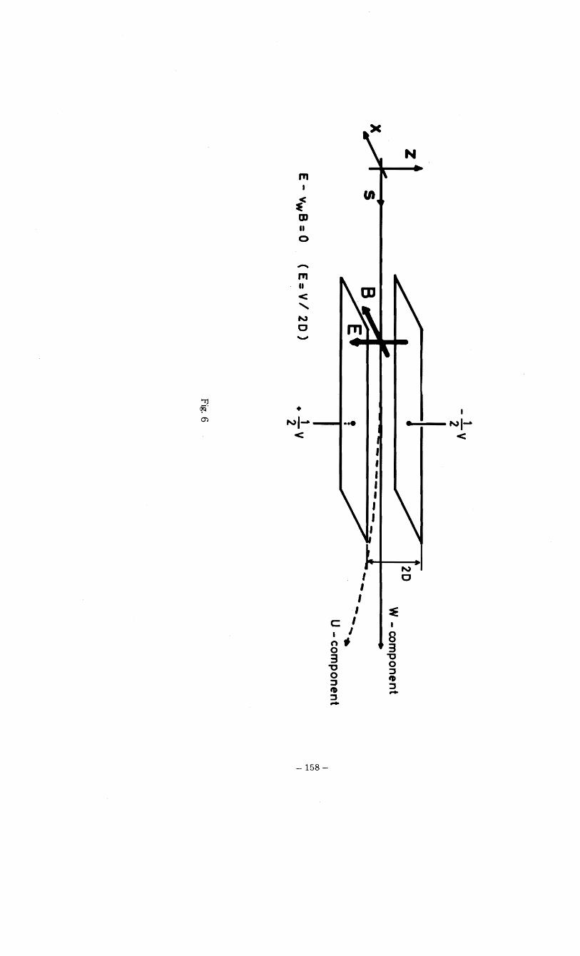
II 1 - c Separator

There are used many kinds of separators in the world. But today I will explain only on the DC

separator which is now under construction at our laboratory. A DC separator is a vacuum chamber in which

an anode and a cathode are located. A very strong electric field, from about 50 to 100 kV / cm, is realized in

the space between the two electrodes, and bends each particle in the beam by some angle which depends on

the velocity of each particle. So we can separate different kinds of particles which has different masses if the

momentum of beam is defined with bending magnet and slit system.

Pr~ctically we use also a magnetic field perpendicular both to the electric field and the beam direction,

and make only wanted particles go straight. Unwanted particles are rejected with the slit located at the

next focus. Schematics of DC separator is shown in Fig 6.

We sometimes use a difinition of the separation vector which shows amount of separation between

wanted particles and unwanted particles in the phase space. The separation vector is

S = (Jz, JZ/)

::: ( -} rE 1 2, - rE 1 )

(2.17)

where r= ;c (.8u

Q =....Y... of unwanted particle. I-'u C

You must watch at the fact that the spacial separation J y is proportional to the electric field strength and to

sq uare of the length of the electric field. But the most important fact is that the spacial separation is

proportional to the r-function which is propotional to inverse cube of the momentum at high energy. These

facts make the particle separation almost impossible at high energy.

II - 2 Beam Design As A System

It is an important purpose for a designer of beam line to get proper intensity, image size or parallelity

of beam and so on. Among them beam intensity is the most essential property for experimenters.

Flux of secondary particles is represented as

d2 N JpF=-- sItJD--pexp(-L/L ) (2.18)dpdQ p 0

where 1:d~ is production rate of secondary particle. at the target; I intensity of primary proton beam;

t target efficiency ; s transmission factor; J D solid angle ;~ momentum bite; p central momentum ; exp p

(-L/L ) decay factor; L beam length; and L =Lc't'decay length of unstable particle. o 0 m Among these parameters, I will explain about some of them.

-147

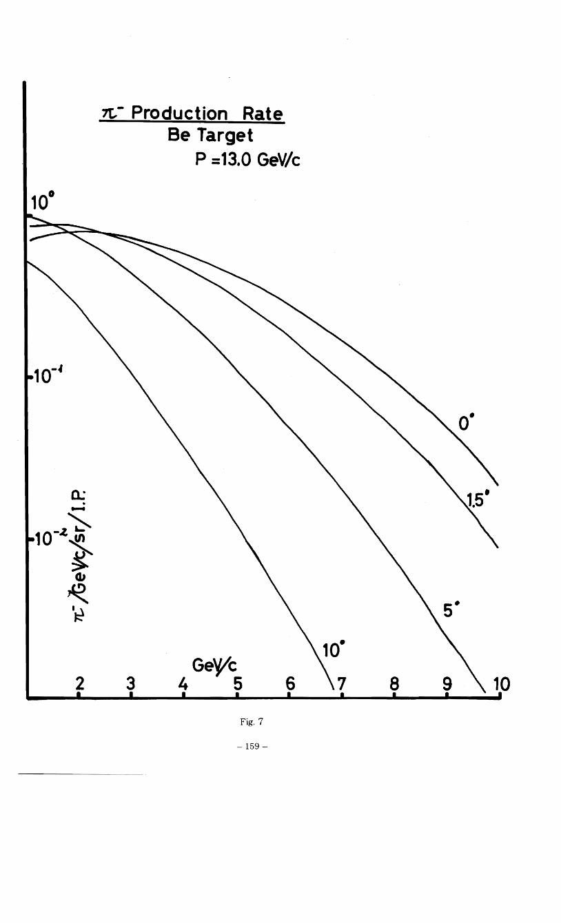
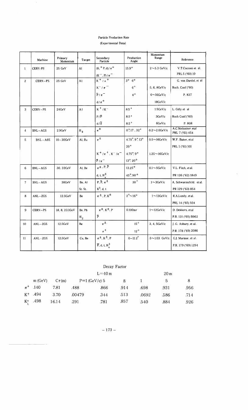
U-2-a Particle Production Rate

When a high energy accelerator was constructed, the first experiment was secondary beam survey,

that is, measurements of production rates of many kinds of secondary particles. Those data are compiled

in table I. This is, of course. not a complete list. In the table, the higher energy data than that of Serpukhov

are excluded.

We can estimate the production rate for our KEK case from these data. But there are some

inconsistencies among them, and these data do not cover all angular and energy region which we need.

On the other hand. some people have tried to describe these data in theoretical and empirical formula.

They are;

1. Cocconi' s formula

d 2 N n lr T l 2

dpd,Q =21r p2 ( T) (2.19) o

where n'lr is mean multiplicity of pion, T mean energy of pion, p laboratory momentum of pions, 2p 0

mean transverse momentum and (J laboratory production angle of pions.

This formula was used as a stant point by other peoples.

2. Trilling's tormula

He assumed that low energy pions were produced by statistical boil-off process and that high energy

pions were decay products of isobars produced at forward angle.

(2.20)

where p is momentum ofsecondary particle, Po momentum of pnmary proton, (}laboratory angle of secondary

particle, and Al to A 3 , BI to B 3 parameters.

4) Ranft's formula

He parametrized all exponents of p, Pi and (} in Cocconi' s formula.

5) Sanford & Wang's formula

They approached not physically but in pure mathematical way, giving attention to the angular dependence

and the energy dependence of the forward production rates of the experimental data from 10 to 30 GeV / c.

C (Jm (p - C p, cos C. (J) J (2.22)6 7

-148 ­

where C to C and m are parameters and m is practically unity;1 8

The last formula represents all data the most nicely. From now I will always use this formula when

I estimate the production rates at our laboratory.

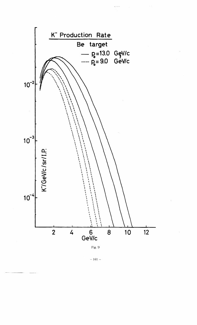
I will give you some examples of the production rates caluculated with Sanford-Wang's formula.

They are given in Figs7, 8 and 9.

II - 2 - b Beam Separation

As I mentioned in II-l-c, it is very difficult to separate high energy particles. In principle it may

be possible to separate them with longer separator. But longer separator requires longer beam length which

increase decay of unstable secondary particles.

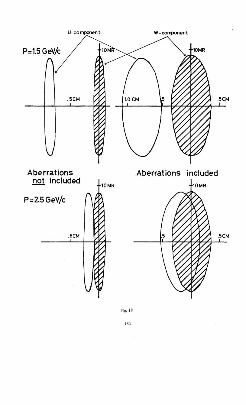
I will give you an example of beam separation in Fig -10. It shows the separation between pions and

kaons in the KEK-K2 beam which will be explained below. In the left-hand side of the figure, aberrations are

are not included and it seems that kaons are nicely separated from pions. But they are hardly separated at

momentum of 2.5 GeV / c in the right- hand side where aberrations are concerned. When physical separation

is not enough, the transmission factor (c) must be decreased to yield an enough ratio of wanted particle to

unwanted particle.

II - 2 -c Decay Loss

Most of secondary particles decay in a short time. For example, charged pions, charged kaons and

long lived neutral kaons have mean lives of 2.60 X 10 - 8 sec, 1.24 X 10- 8 sec and 5.172 X 10- 8 sec,

respectively. So their charactristic decay lengthes are, respectively, 7.81 m, 3.70 m and 16.14 m.

Decay factor is given by

fd = exp (- L/Lo ) (2.23)

where L =....E... CT. L represets relatiristic prolongation. Decay loss is not serious for high momentum o m m

particles and also for lighter particles. Then this problem is the most serious in charged kaon beam lines,

especially in low momentum kaon beam lines.

I will give a result of short calculation for you to have a rough image in table II.

-149 ­

I I I KEK Beam Magnets and DC Separator

We have designed some elements for KEK beam lines. You will use these elements in a few years.

So I will introducelyouJhem here.

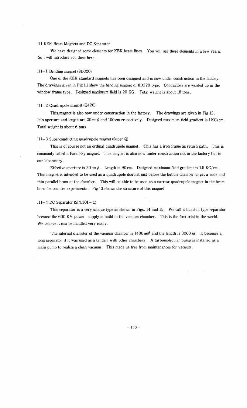
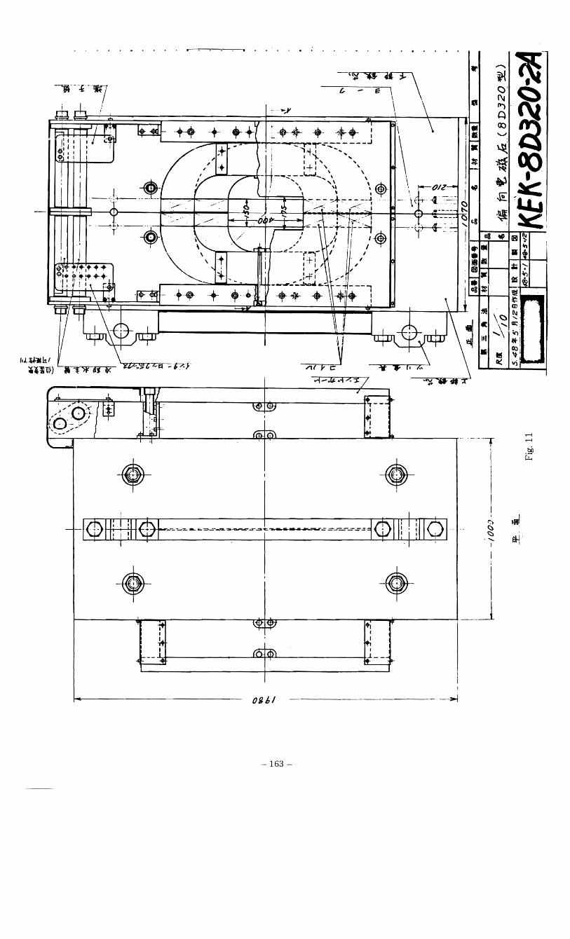
111-1 Bending magnet (8D320)

One of the KEK standard magnets has been designed and is now under construction in the factory.

The drawings given in Fig 11 show the bending magnet of 8D320 type. Conductors are winded up in the

window frame type. Designed maximum field is 20 KG. Total weight is about 18 tons.

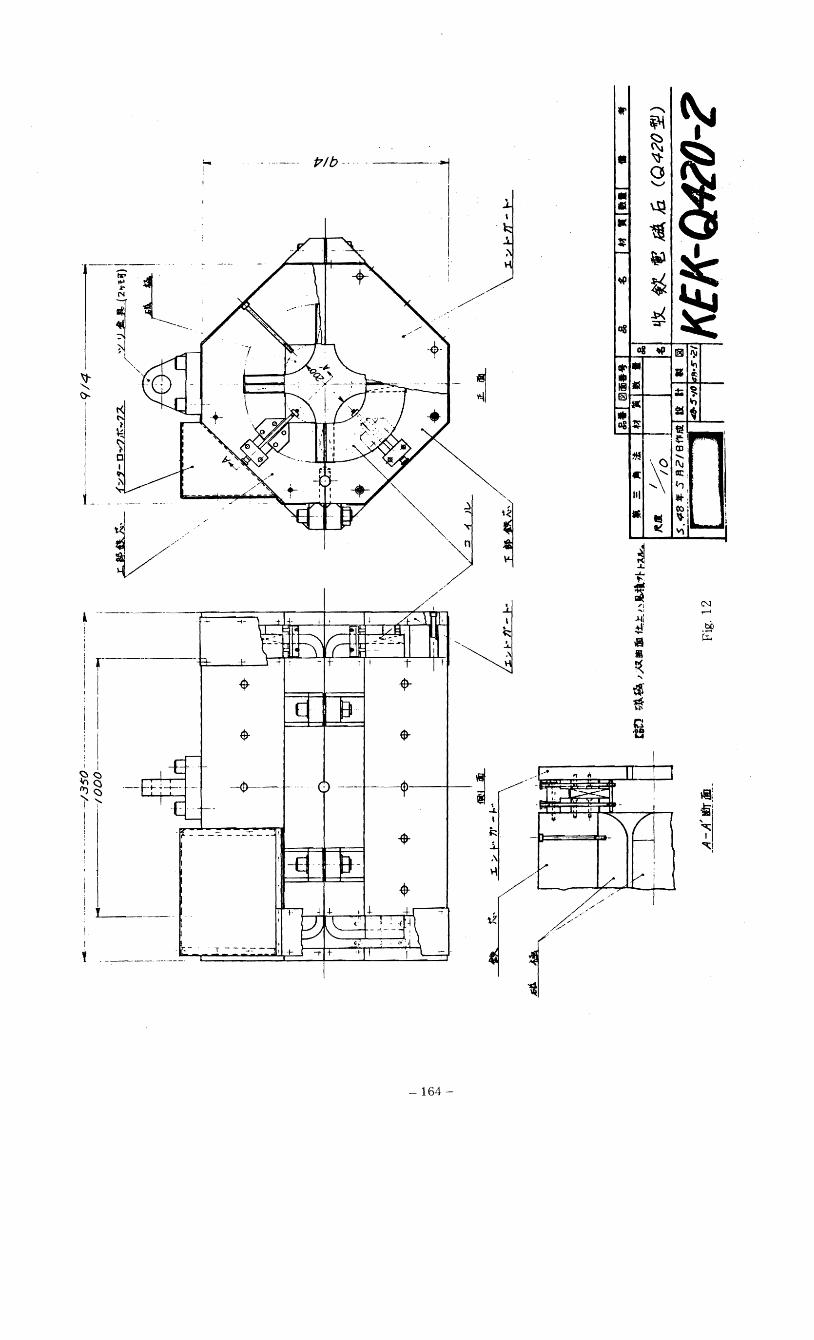
111-2 Quadrupole magnet (Q420)

This,magnet is also now under construction in the factory. The drawings are given in Fig 12.

It's aperture and length are 20 cm if> and 100 cm respectively. Designed maximum field gradient is 1 KG/ cm.

Total weight is about 6 tons.

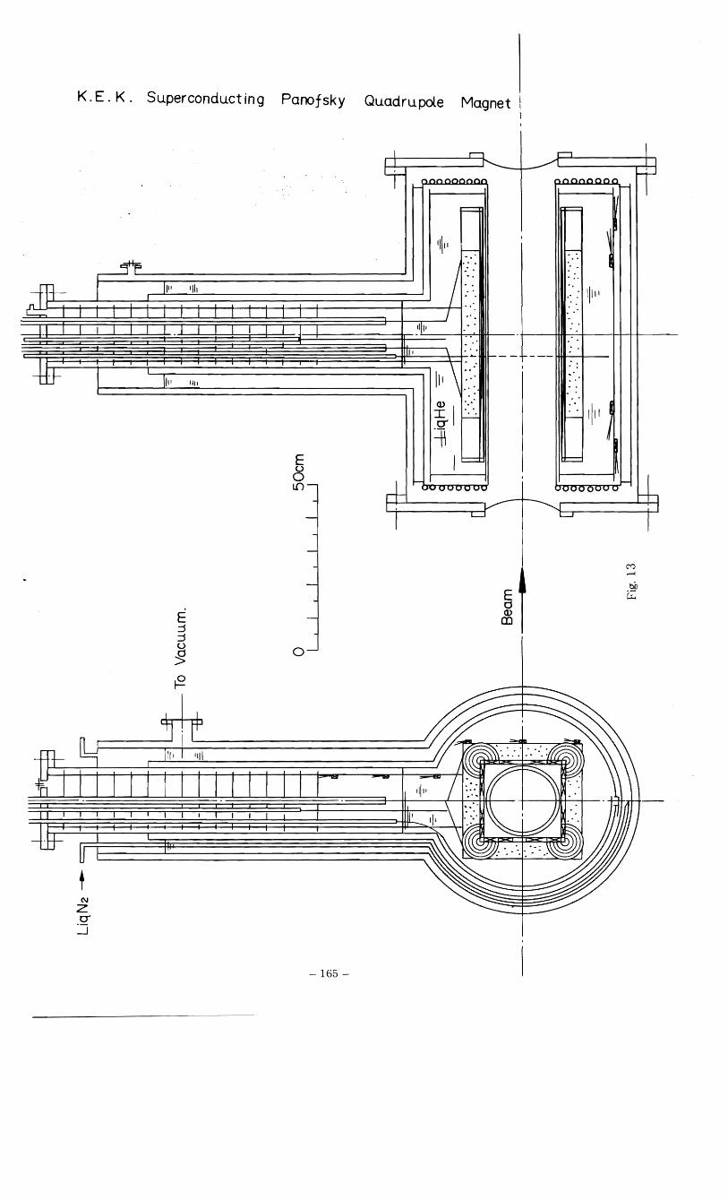
111-3 Superconducting quadrupole magnet (Super Q)

This is of course not an ordinal quadrupole magnet. This has a iron frame as return path. This is

commonly called a Panofsky magnet. This magnet is also now under construction not in the factory but in

our laboratory.

Effective aperture is 20 cm if> . Length is 90 cm. Designed maximum field gradient is 1.5 KG/ cm .

This magnet is intended to be used as a quadrupole doublet just before the bubble chamber to get a wide and

thin parallel beam at the chamber. This will be able to be used as a narrow quadrupole magnet in the beam

lines for counter experiments. Fig 13 shows the structure of this magnet.

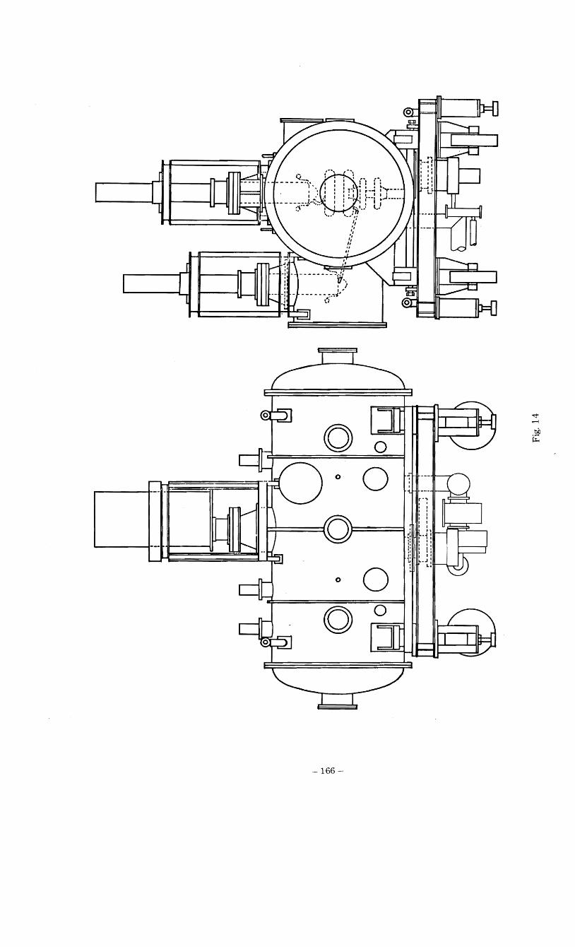
I I 1-4 DC Separator (SPL301- C)

This separator is a very unique type as shown in Figs. 14 and 15. We call it build·in type separator

because the 600 KV power supply is build in the vacuum chamber. This is the first trial in the world.

We believe it can be handled very easily.

The internal diameter of the vacuum chamber is 1400 _if> and the length is 3000 _. It becomes a

long separator if it was used as a tandem with other chambers. A tarbomolecular pump is installed as a

main pump to realize a clean vacuum. This made us free from maintenances for vacuum.

-150 ­

IV KEK Experimental Beams

IV -1 Brief Sketch of the KEK - PS

The maximum energy of the KEK accelerator is 8 GeV at the first stage and will be escalated up to

12 GeV in 1977. The intensity was designed to be 10 13 ppp at repitition rate of 0.5 pps

This machine is of a Quadrant type and so has four straight sections. The first straight section (S 1)

is for the injection from the booster synchrotron. The fourth straight section (S4) is for the RF acceleration.

The remained two straight sections (S2 and S3) are used to extruct proton beams. At the S2 section a short

spill beam is ejected for bubble chamber experiments. and a long spill. beam for counter experiments is

extructed at the S3 section. Details of a short spill beam were described in the KEK Annual Report of 1971.

A long spill beam is yet at the stage of study.

IV - 2 Secondary Beams

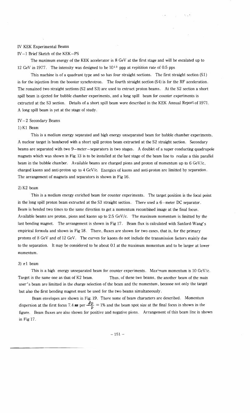
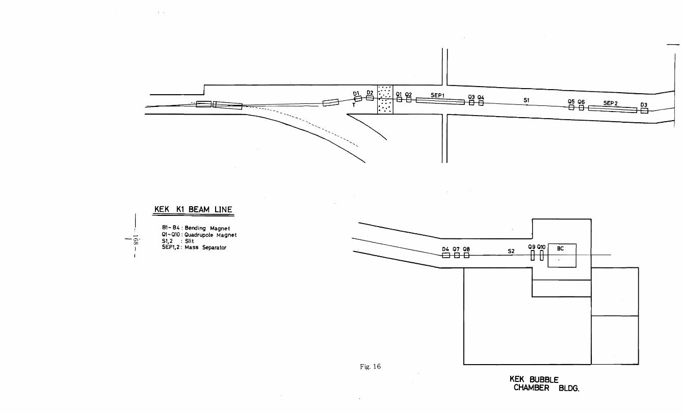
1) K1 Beam

This is a medium energy separated and high energy unseparated beam for bubble chamber experiments.

A nuclear target is bombered with a short spill proton beam extructed at the S2 straight section. Secondary

beams are separated with two 9-meter-separators in two stages. A doublet of a super conducting Quadrupole

magnets which was shown in Fig. 13 is to be installed at the last stage of the beam line to realize a thin parallel

beam in the bubble chamber. Available beams are charged pions and proton of momentum up to 6 GeV/c.

charged kaons and anti-proton up to 4 GeV/c. Energies of kaons and anti-proton are limitted by separation.

The arrangement of magnets and separators is shown in Fig 16.

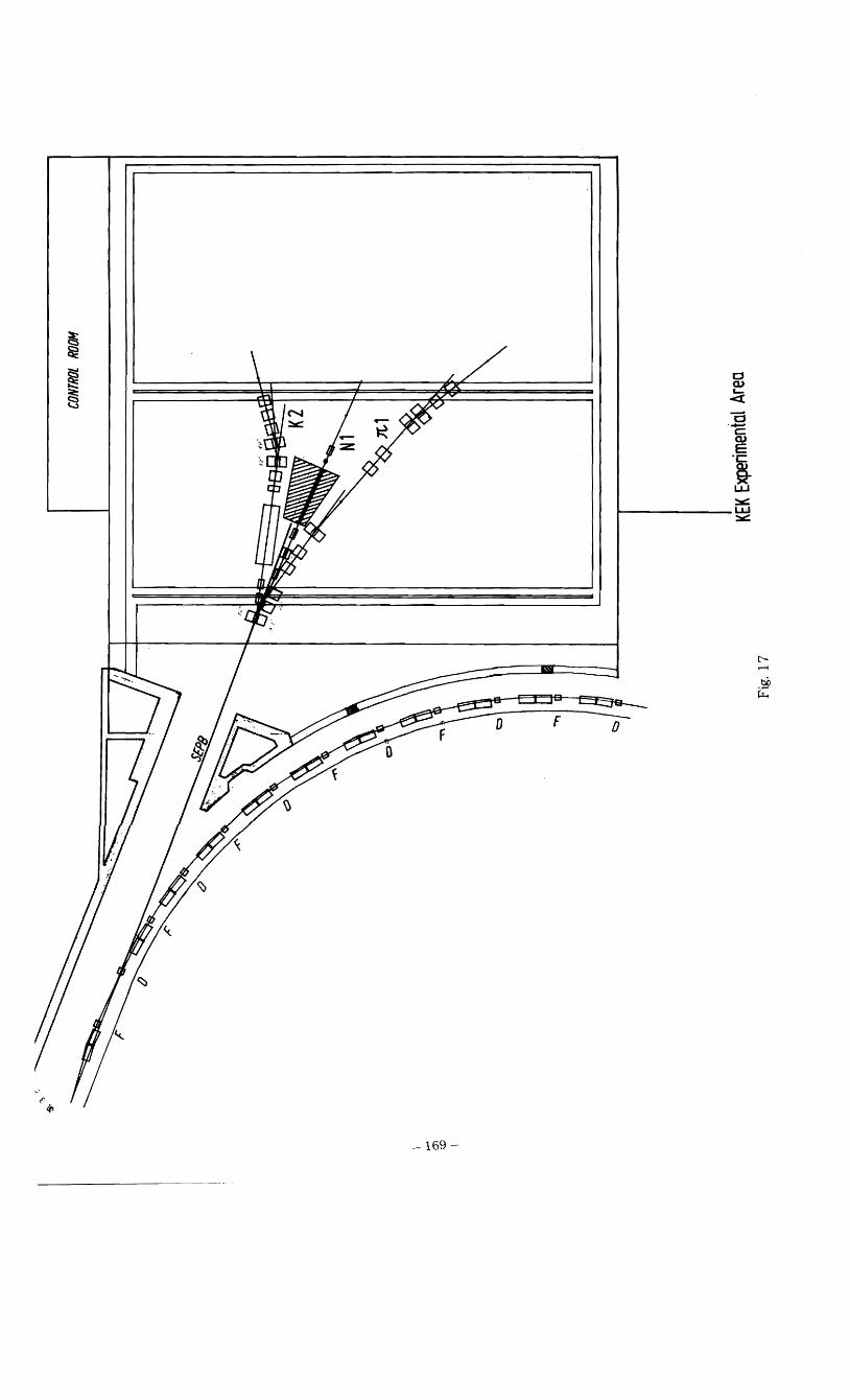
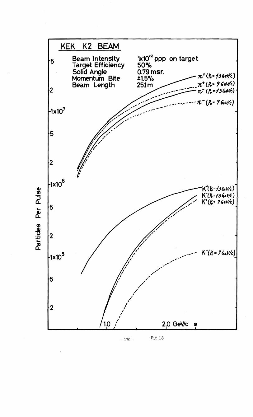
2) K2 beam

This is a medium energy enriched beam for counter experiments. The target position is the focal point

in the long spill proton beam extructed at the S3 straight section. There used a 6-meter DC separator.

Beam is bended two times to the same direction to get a momentum recombined image at the final focus.

Available beams are proton. pions and kaons up to 2.5 GeV Ic. The maximum momentum is limitted by the

last bending magnet. The arrangement is shown in Fig 17. Beam flux is calculated with Sanford -Wang's

empirical formula and shown in Fig 18. There. fluxes are shown for two cases. that is. for the primary

protons of 8 GeV and of 12 GeV. The curves for kaons do not include the transmission factors mainly due

to the separation. It may be considered to be about 0.1 at the maximum momentum and to be larger at lower

momentum.

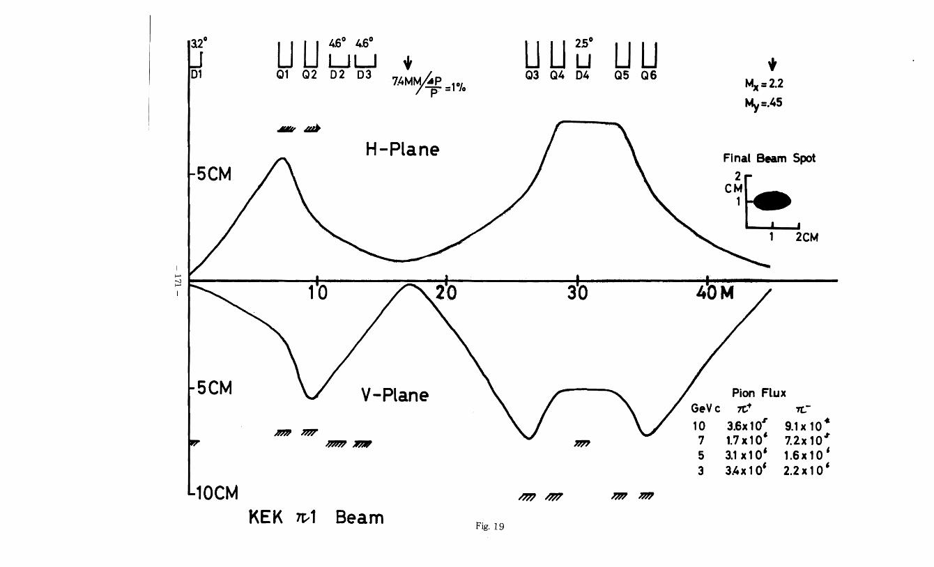
3) reI beam

This is a high energy unseparated beam for counter experiments. Max;mum momentum is 10 GeV / c.

Target is the same one as that of K2 beam. Thus. of these two beams. the another beam of the main

user" s beam are limitted in the charge selection of the beam and the momentum, because not only the target

but also the first bending magnet must be used for the two beams simultaneously.

Beam envelopes are shown in Fig. 19. There some of beam characters are described. Momentum

dispersion at the first focus 7.4 1!I1R per ~ 1% and the beam spot size at the final focus is shown in the p figure. Beam fluxes are also shown for positive and negative pions. Arrangement of this beam line is shown

in Fig 17.

-151 ­

-------------- _.__ ... - ­

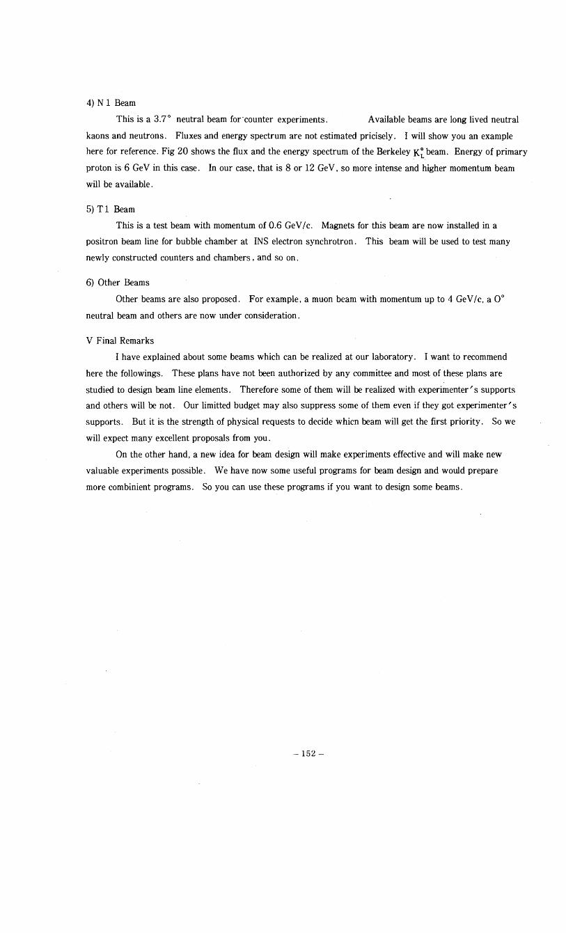
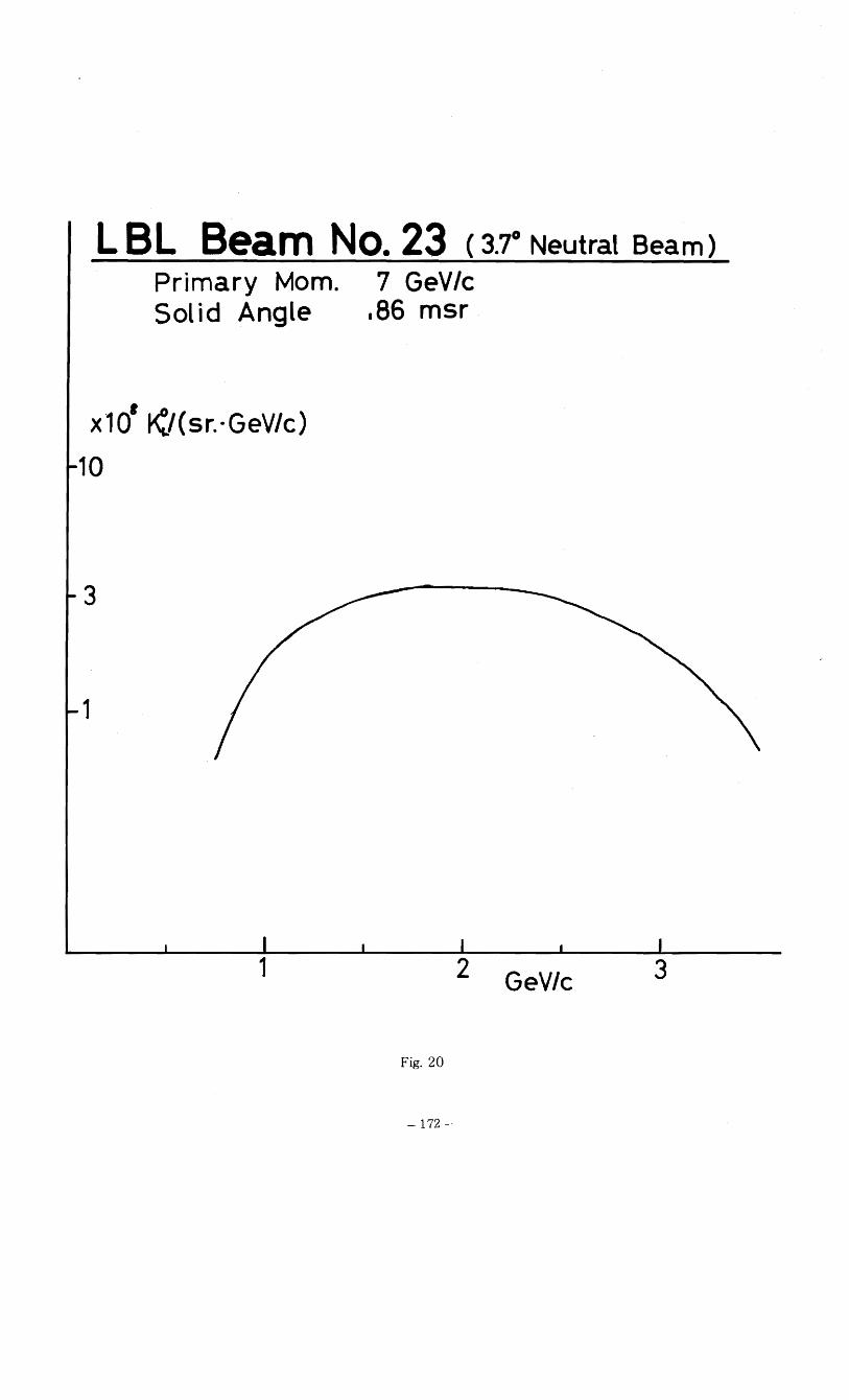
4) N 1 Beam

This is a 3.7 0 neutral beam for'counter experiments. Available beams are long lived neutral

kaons and neutrons. Fluxes and energy spectrum are not estimated pricisely. I will show you an example

here for reference. Fig 20 shows the flux and the energy spectrum of the Berkeley K~ beam. Energy of primary

proton is 6 GeV in this case. In our case, that is 8 or 12 GeV. so more intense and higher momentum beam

will be available.

5) T1 Beam

This is a test beam with momentum of 0.6 GeV/c. Magnets for this beam are now installed in a

positron beam line for bubble chamber at INS electron synchrotron. This beam will be used to test many

newly constructed counters and chambers, and so on.

6) Other Beams

Other beams are also proposed. For example. a muon beam with momentum up to 4 GeV/c, a 0°

neutral beam and others are now under consideration.

V Final Remarks

I have explained about some beams which can be realized at our laboratory. I want to recommend

here the followings. These plans have not been authorized by any committee and most of these plans are

studied to design beam line elements. Therefore some of them will be realized with experimenter's supports

and others will be not. Our limitted budget may also suppress some of them even if they got experimenter's

supports. But it is the strength of physical requests to decide whicn beam will get the first priority. So we

will expect many excellent proposals from you.

On the other hand, a new idea for beam design will make experiments effective and will make new

valuable experiments possible. We have now some useful programs for beam design and would prepare

more combinient programs. So you can use these programs if you want to design some beams.

-152

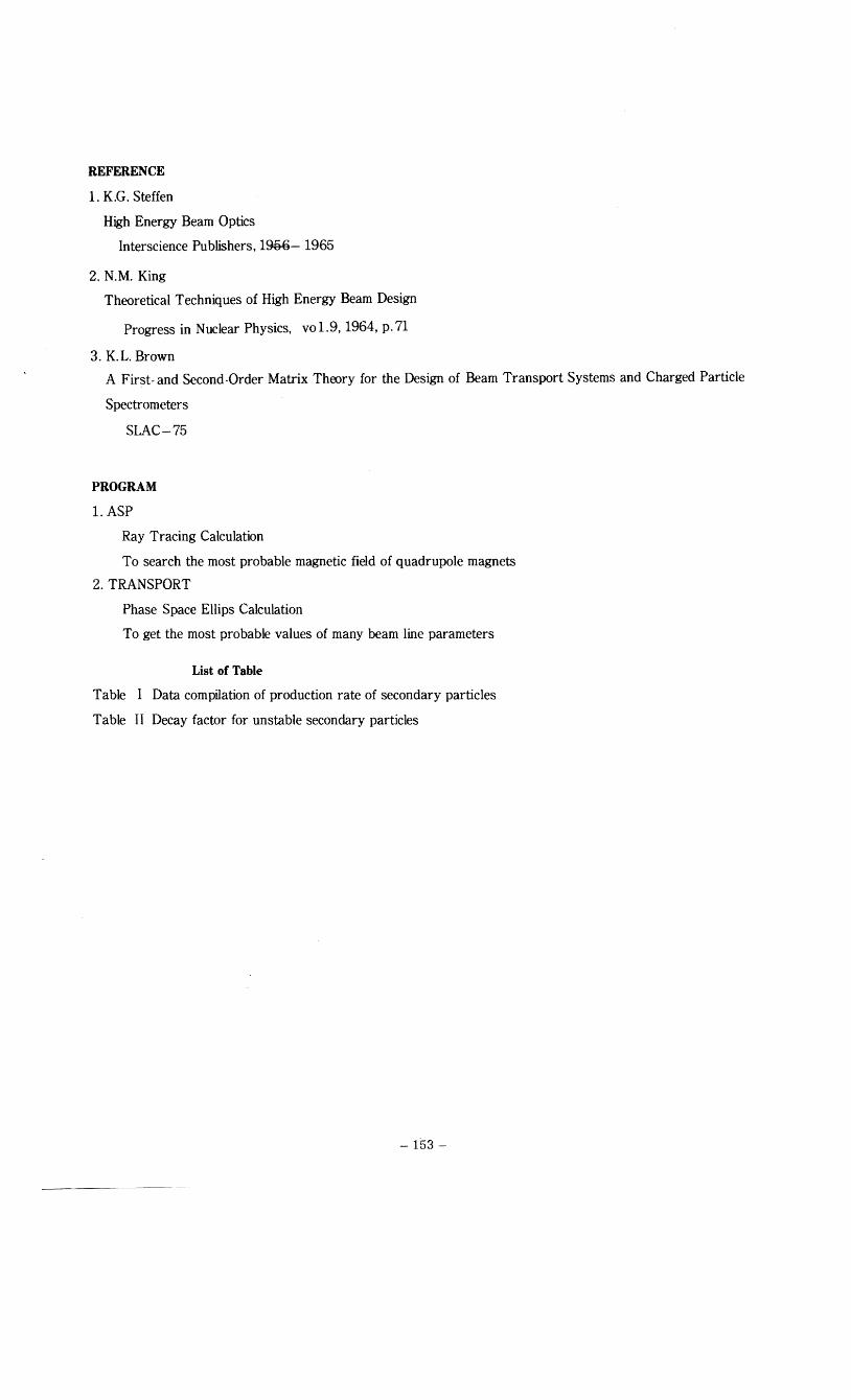
REFERENCE

1. K.G. Steffen

High Energy Beam Optics

Interscience Publishers. I9&{;- 1965

2. N.M. King

Theoretical Techniques of High Energy Beam Design

Progress in Nuclear Physics, vo1.9, 1964, p.71

3. K. L. Brown

A First- and Second -Order Matrix Theory for the Design of Beam Transport Systems and Charged Particle

Spectrometers

SLAC-75

PROGRAM

I.ASP

Ray Tracing Calculation

To search the most probable magnetic field of quadrupole magnets

2. TRANSPORT

Phase Space Ellips Calculation

To get the most probable values of many beam line parameters

List of Table

Table Data compilation of production rate of secondary particles

Table II Decay factor for unstable secondary particles

- 153

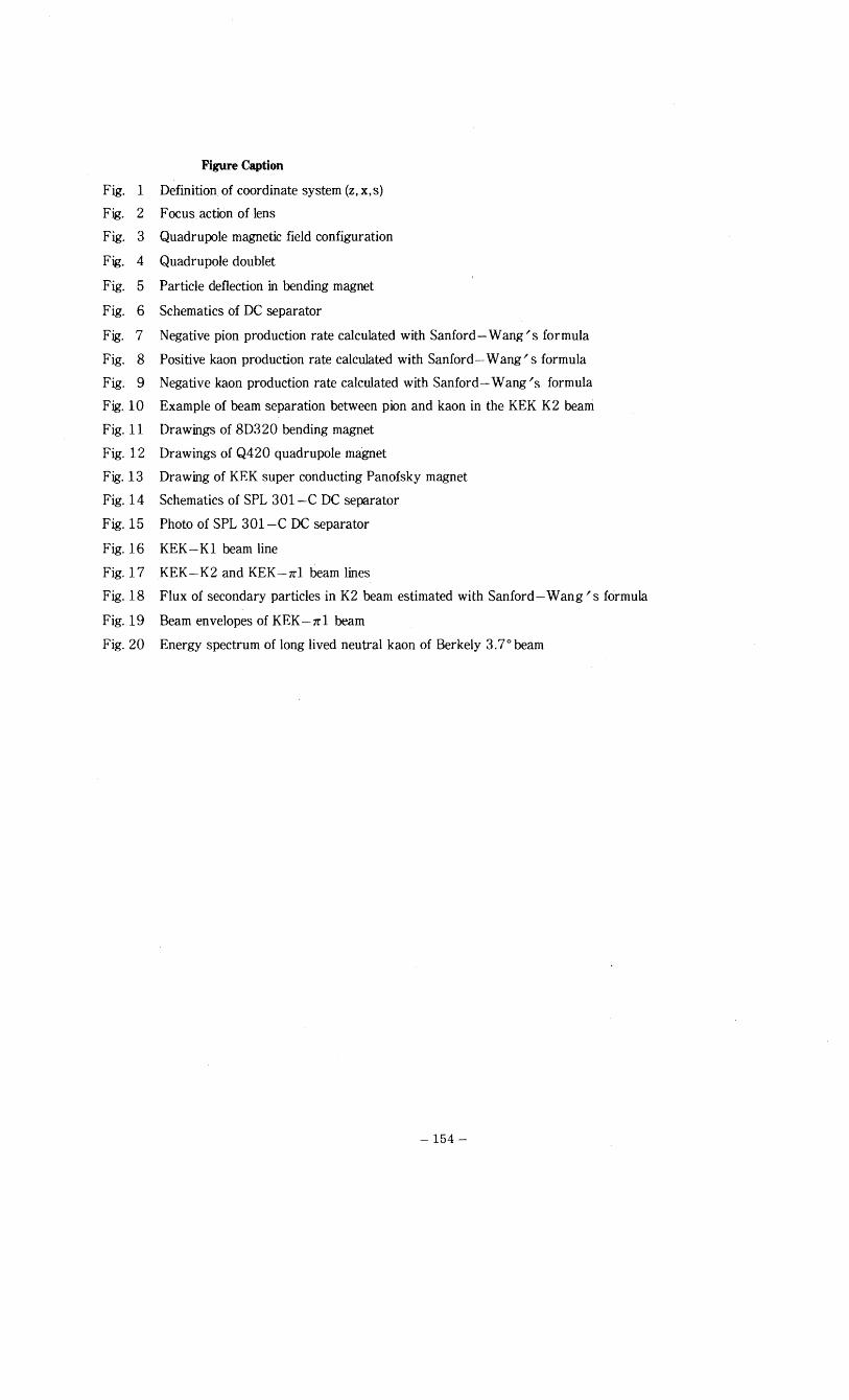
Figure Caption

Fig. 1 Definition of coordinate system (z, x,s)

Fig. 2 Focus action of lens

Fig. 3 Quadrupole magnetic field configuration

Fig. 4 Quadrupole doublet

Fig. 5 Particle deflection in bending magnet

Fig. 6 Schematics of DC separator

Fig. 7 Negative pion production rate calculated with Sanford - Wang's formula

Fig, 8 Positive kaon production rate calculated with Sanford - Wang's formula

Fig. 9 Negative kaon production rate calculated with Sanford - Wang's formula

Fig.l0 Example of beam separation between pion and kaon in the KEK K2 beam

Fig. 11 Drawings of 8D320 bending magnet

Fig. 12 Drawings of Q420 quadrupole magnet

Fig.13 Drawing of KEK super conducting Panofsky magnet

Fig.14 Schematics of SPL 301-C DC separator

Fig. 15 Photo of SPL 301-C DC separator

Fig.16 KEK-Kl beam line

Fig.17 KEK-K2 and KEK-i!1 beam lines

Fig. 18 Flux of secondary particles in K2 beam estimated with Sanford - Wang's formula

Fig. 19 Beam envelopes of KEK -i!1 beam

Fig. 20 Energy spectrum of long lived neutral kaon of Berkely 3.7 0 beam

-154 ­

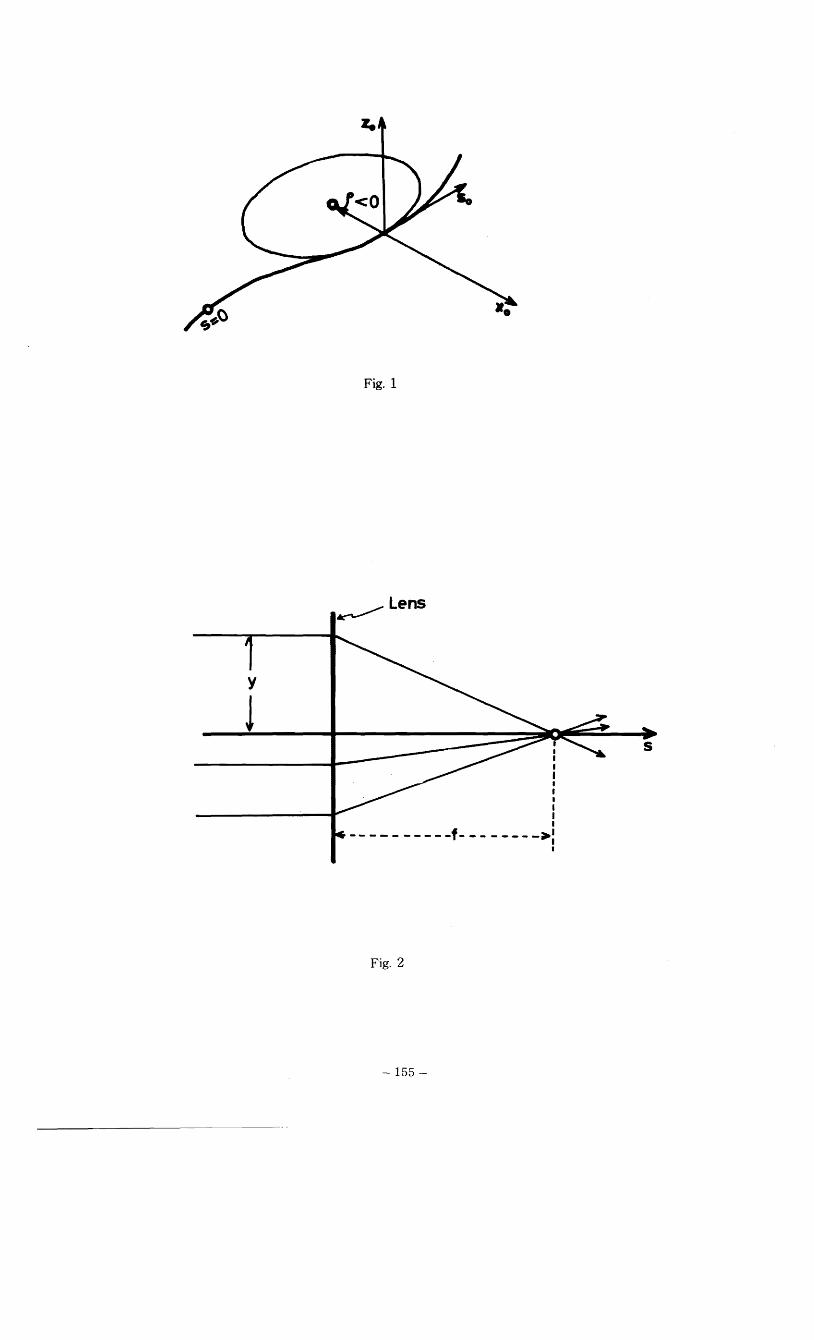
Fig. 1

I

•I I I•I•

__ - I

- - - - - - -f - - - - - - - _;...1:I I

Fig. 2

- 155

:z

Fig. 3

-f. + fa, i ..--d---++---- -X----~-d~---.,V-PLANE

..,. ...... ......, ...... I I I

z; I I I, I

H-PLANE

•t ... I -.......

,I t

---E-------~ I I -------1- - - -- ~!

II

:~-- -- --0- - --I

F

Fy =VF

~ =VF

I I

-f.& Fig. 4

156 ­

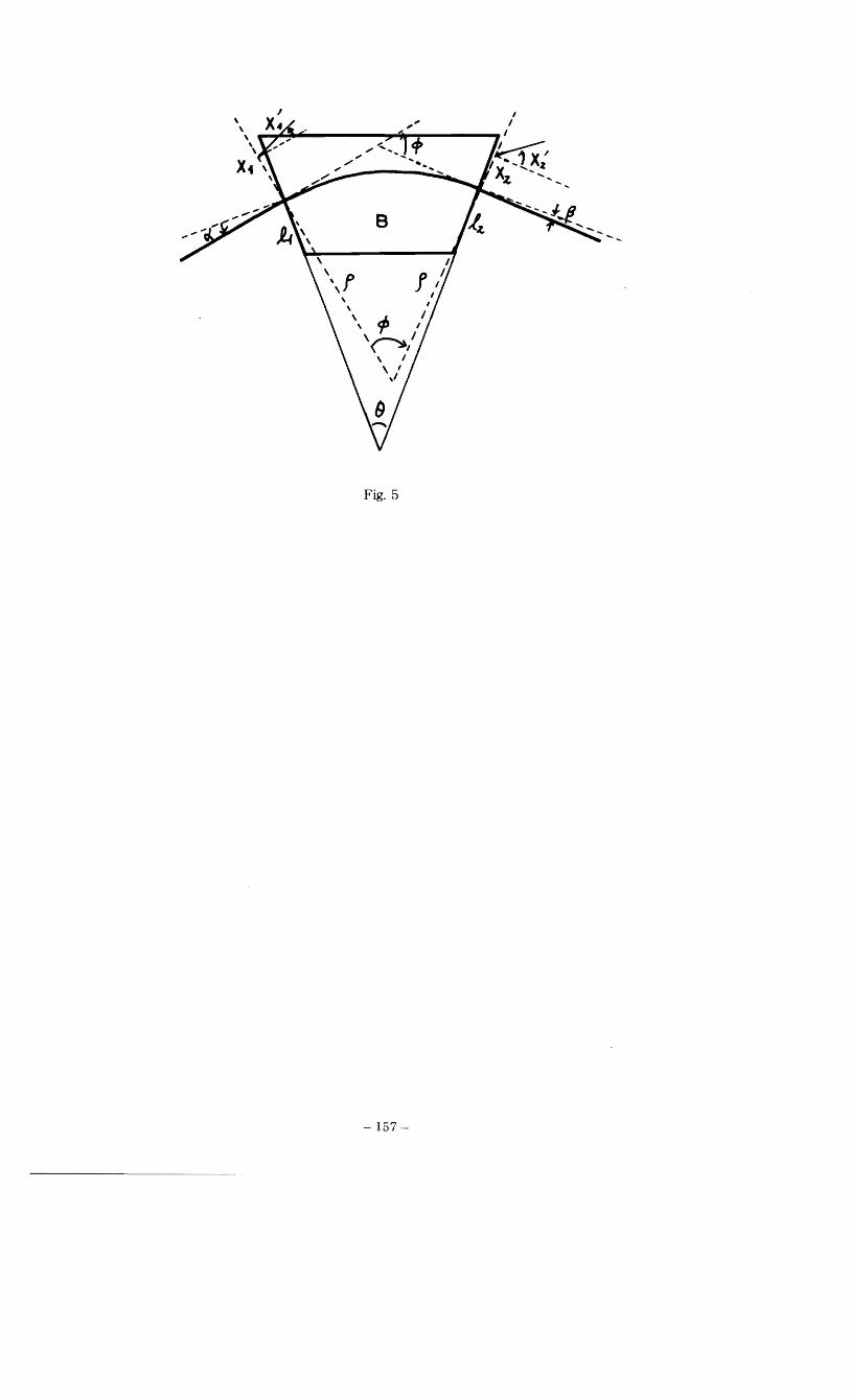
Fig. 5

157

fI1

I OJ II 0

........ fI1.1 <

N" C .......,

• NI-_.....··•

<

,I ,I

c: I I In'o 3

"0 o :::I to :::I...

-158 ­

N

...--NI-I

<

N C

~ I

8 3 "0 o :::I to :::I...

7L- Production Rate Be Target

P =13.0 GeV/c

2 3 Ge'f'c

4 5

Fig. 7

159 ­

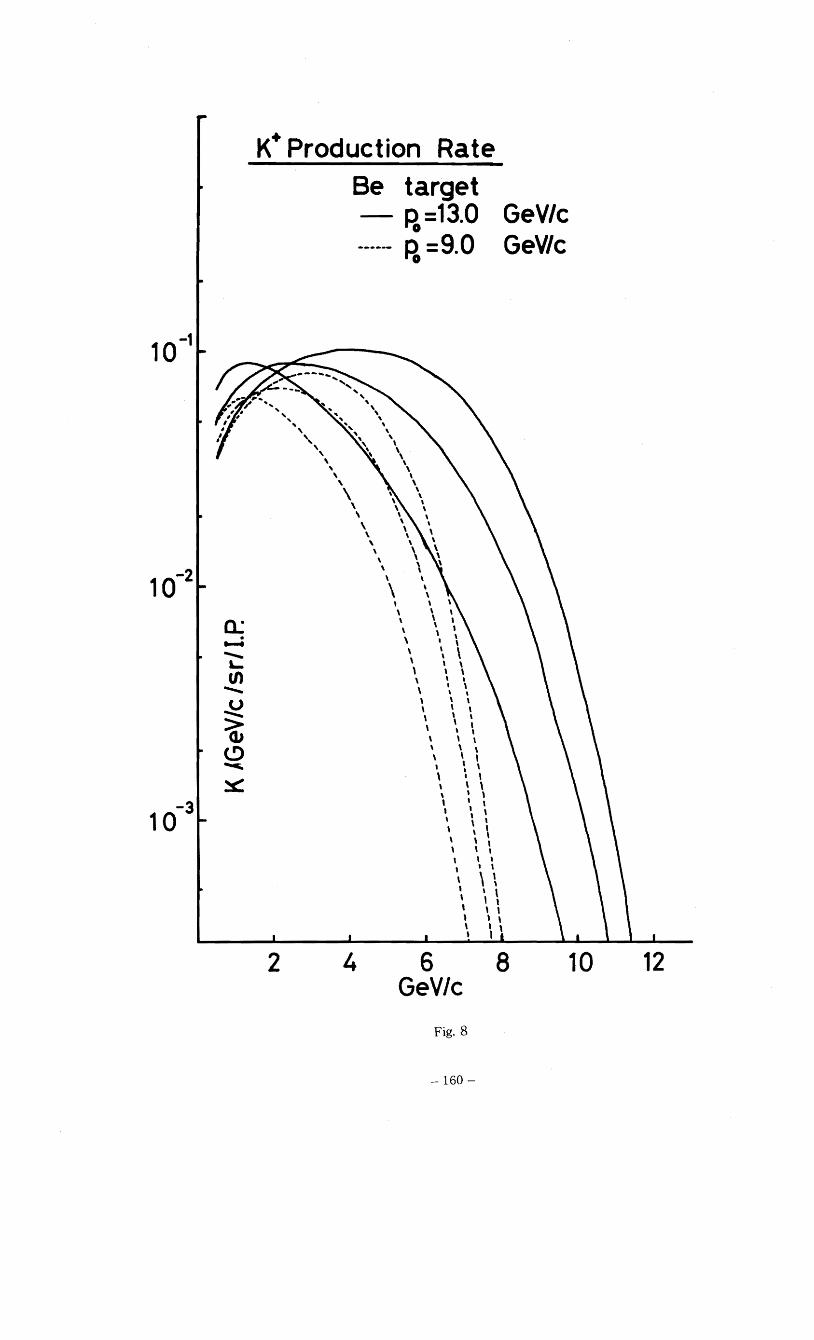
K+ Production Rate

Be target R=13.0 GeVlc o

Po =9.0 GeV/c

10-2

a.:...... .....-.. L.. en .....-.. ~ ~ <.!) ........ ~

10-3

\ \

\

\ , \, \

\ \ \ \

\ \ \ \ , \

,,\ \, \

\ ,

\ ,,

\, \ \, \ \, \ , \

\ ,, , \ \ \ \ \ \ \ \ , t \ \ \ ' ,, , \ \ ' ,t ' \, ' \, t ,

\ \ , \ \

\ , t, , t , t

t ' ,, \ \, , \, , ,, , ,, , ,, , \, 1

2 4 6 8 GeV/c

Fig. 8

160 ­

10 12

Po =9.0 GeV/c '1~.'""'~",~"'''- " ..... "',

c..:. ...... ......... L.. Ul

\ \ \

\ \,

2

, \ \ \ \,\ \ \

\ \ \ \ ,\ \ \ \ \ ,\ \ \ \ \ \ \ \ \ \\ \ \ , \ \

\ ,\ \ \ \

\ " \ ,\, \ \ \ ,\ \ \ \ \ \ \ \ \ \ \ \ \ \ \ \ \ , \ \ \ \\ \,

4

, \ \ \ '\, \, \ '\\ \ \

\ ' \, \ , \ \ \ \ \ \ \ \ \ , ,\ , ,\, \ \

\ \"\ , ,, ,\, , \ , , \

\ '\\ , \ , \ \ \ , , , \ \ \ \ , \ \ \ , ,\ \ \\ , ,, \ \

'. ~ \, \, , , \ ,

\ \ ,, \ \ , \ \ \ \' \ \'

, \"\ ,

6

K- Production Rate

Be target

Po =13.0 G,Vlc

GeV/c Fig. 9

161 ­

8 10 12

P=1.S GeV/c

.5CM 1.0 CM

Aberrations Aberrations included not included

.5CM

10MR

Fig. 10

162

,.--:f---.n

/i i

!

11!~...bJ .lllt) n-w-wv­

-+

_-,;:--\_~___'"U' 4~ (, - T\

\

\

r--tJ/Z

\~ --t

:.J:­ At : ­~-

.­ .­

I I;'"I

- <:) t-..

08

------T

I I

I I I

I

I

r----.r-~-----ntd~----,...,..--.ir----t, _____J

"""" ~-rt <:)'

~ f\i I\')

A «> a'-"

~ ~ 'P~

~ ~~ ~ '-1.1...1

'\1 ~;i

'" B~ ~

~I,

--------;...j0961

163

frlb ­ --I

I

~.l~~, ~,

"

~ <>­I I

t I

,I

-164 ­

K. E. K. Superconduct ing Panojsky Quadrupole Magnet

I II c:J 1I , 1 1 , I

T -­~"\nonnono

l- t--'

F= F= ~

'11" I \

---:­ r:-:­-. .--5~ /

" . , ,- '·. · .. '.

~ \i" 'II! · . 11111

1 I 1 I J 1 t I I J 1 I J J .' .. :'11' · .==rJ I I 1 I J 1 1 .1 I I I J 1 I I

" -I----­. 1111' \ . ' . ..... --­ 1---­..l. . ,

-W . . III \

. · . ,

lip .' · '1111 .' . · . . . . .

~I ' . , .

IIII · .r-:-..:. r-­

i ~

E It::::= 1== ~()

~ 0 I

r-r+ I-­L()­ OQ·Ouoou~ IJUUVOVVV

- 1 I J J - I 1.....-1 L..J

I--

M

-165 ­

co 0

0 0 .. · ·

r-~

I I I I I I, tl ...

I .J I

"', II

" . III,

!: I II I I, 1 II

l! , II

:.. ... .J :

· 0 I L.

0

co

-.:::r r-I

.~ Ii;..

166

Fig. 15

167

-...............

52 Q9 Q10 J Be

SEP1 Q3 Q4 51 Q5 Q6 SEP2

KEK K1 BEAM LINE

81- B4 : Bending Magnet I---' Q1-Q10: Quadrupole Magnet (1)­00 51,2 : Slit

SEP1,2: Mass SeparatorI

Fig. 16

KEK BUBBLE CHAMBER BLDG.

169 ­

KEK K2 'BEAM

5

5

6lx10

CII en-::J 0.. ... .,~

Beam Intensity Target Efficiency Solid Angle Momentum Bite Beam Length

~

~'" K"(r,· '~vk)~

K+(P.:: IJ .vle) K-{A:(J_~v,i)

CII ~"'~ 0.. .I~

/ ~

/en .I

.I~~JIl .~....., 2 ,I'

I'

... ,I',,0.. I "'

/ I

........ .".- K -(I:, • , ~..v/c)I .".""

I ,,'" I

I ",' "

I I,

I I

I I

I

.I' ~'"

"'~ .I

,.1 ,

1'1' I' ,I' ,

I I

I I

2 I I

1x105

I I

I I

I I 2.0 GeV/c Q

Fig. 18-170 ­

12°

UU~~ uur; uu t+01 Q1 Q2 02 D3 Q3 Q4 04 Q5 Q6 7.4Mi'1 =1 010 Mx =2.2

My =.45

..., ~ H-Plane

/\.. Final Beam SpotSCM

2~eM

1 1 2eM

~ r 1'0 ~2'o

SCM V-Plane

,1J?I'} ""

Pion Flux GeV c "ft,+

10 3.6x lOr, 1[,. ­

3'0 4bM ~

9.1 X 10 ...

IJ"J'J'}? .. 7 1.7xl0 7.2x 10'""" 5 11 xl0' 1.6x 10 I 3 3Ax 10' 2.2 X10'

/J'I') I?)? HI? J'JJ'I

KEK 7Vl Beam Fig. 19

LBL Beam No. 23 (3.70 Neutral Beam) Primary Mom. 7 GeV/c Solid Angle .86 msr

x10' 't¢(sr. · GeVlc)

10

3

1

1 32 GeV/c

Fig. 20

172

Particle Production Rate

(Experimental Data)

Momentum

Machine Primary Target

Secondary Production Range Reference

Momentum Particle Angle

1 CERN·PS 25 GeV AI (K.+P,d)/rr+ 15.9° 2........ 5.3 GeV/c V.T.Cocconi et al.

(K-, P)/rr ­ PRL 5 ('60) 19

2 CERN-PS 25 GeV Al K+ / n;+ 3° 6° G. von Dardel, et al

K-/rr - 6° 5,6,8GeV/c Roch. Conf ('60)

P Irr ­ 6° 6 ........ 16GeV/c P. 837

d/x+ 18GeV/c

3 CERN-PS 24GeV AI K+ IK­ 8.5° 1.5GeV/c L. Gilly et al

PIP 8.5 ° 3GeV/c Roch Conf ('60)

did 8.5 ° 6GeV/c P.808

4 2.9GeV H2 ± 0~17,32° 0.2 ........ 2.0GeV/c A.C.Melissino,: etal

x PRL 7 ('61) 454

5 BNL-A6S 10-30GeV AI, Be rr± 4.75°, 9~ 13° 0.5....... 16GeV/c W.F. Baker, etal

20° PRL 1 ('61) 101

K+ Ix + ,K- Ix 4.75°,9° 1.25 ........ 16GeV/c

P/rr - 13°,20° .

6 BNL-AGS 30,33GeV AI, Be x±' P, P 13.25 0 0.1"""5GeV/c V.L. Fitch, eta!.

d, t, H3 45~ 90 0 PR 126 ('62) 1849 e

7 BNL-AGS 30GeV Be, Al - ±P,P, x 30° 1"""3GeV/c A, Schwarzschild, eta!.

St. St. Kl, d, t PR 129 ('63) 854

8 ANL-ZGS 12.5GeV Be rr±,p,K± 2°"""16° 1"""13GeV/c R.A.Lundy, eta!.

PRL 14 ('65) 504

9 CERN-PS 18,8, 23.1GeV Be. Pb x±.K±,P 0.100mr 1....... 12GeV/c D. Dekkers, et al

Hz p P.R. 131 ('65) B962

10 ANL-ZGS 12.5GeV Be x±· 15 ° 3.4,5GeV/c j. G. Asbury, et al.

rr+ 12° P.R. 178 ('69) 2086

11 ANL-ZGS 12.5GeV Cu. Be x±,K±,P .5 ........ 1.03 GeV/c GJ. Marmer, et al.

- 3P, d, t, H e

P.R. 179 ('69) 1294

Decay Factor

L=40m 20m

m (GeV) C,(m) P=l (GeV Ic) 5 8 1 5 8

rr+ .140 7.81 .488 .866 .914 .698 .931 .956

K± .494 3.70 .00479 .344 .513 .0692 .586 .714 Ko

L .498 16.14 .291 .781 .857 .540 .884 .926

-173