design of a high data rate audio band ofdm modem · pdf filedesign of a high data rate audio...
TRANSCRIPT
1
Design of a High Data Rate Audio Band
OFDM Modem
A thesis
Submitted to the faculty of the
Worcester Polytechnic Institute
In partial fulfillment of the requirements for the
Degree of Master of Science
in
Electrical and Computer Engineering
By
Abhijit .C. Navalekar
March, 2006
Approved by:
Dr. William R. Michalson, Thesis Advisor
Dr. Jim Matthews, Committee Member
Dr. Peder Pedersen, Committee Member
Dr. Fred Looft, Head Of Department

2
ABSTRACT
Land mobile radio technology (LMR) has existed since the early 1920’s. The most visible
manifestation of this technology is the handheld VHF/UHF radios also referred to as
‘walkie-talkie’. These handheld devices are one of the most ubiquitous forms of radio
communication systems. Most of them are designed for transmitting analog voice signals.
Due to an increase in the amount of digitized analog signals over the past few years
complemented by a need for transmitting pure digital data, there has been a desire to
transmit digital data. There are methods which allow the analog radios to transmit digital
data without any modifications; however the data rate achievable using these methods is
very low. In contrast, the digital variants of these hand-held radios are capable of
transmitting digital data at comparatively higher data rates. However they are expensive
and require major infrastructure overhauls.
In this thesis, a prototype modem is developed, which interfaces with an analog radio
without a requirement for any modifications. Furthermore, the data rates achievable are
comparable with those achieved using digital radios. The modem uses Orthogonal
Frequency Division Multiplexing (OFDM) technique to generate an audio band signal
which is fed to the radio. Thus the digital data is morphed into an audio band analog
signal eliminating any need for modifications to the radio. The OFDM technique used to
generate the audio band signal from data bits ensures maximum bandwidth efficiency.
The developed modem is capable of communicating over Ethernet connection. It uses a
RJ 45 interface to connect to a data source. It is also capable of supporting a host of radio
interfaces. The modem also implements its own version of medium access layer (MAC)
and physical (PHY) layer protocols. There are four versions of modems designed. They
differ in terms of the data rates they can support. Currently, version 1 which supports data
rate of 12kbps has been implemented.

3
ACKNOWLEDGEMENTS
First and foremost, I would like to thank my advisor, Professor William R. Michalson for
his patience, support and guidance without which this project would not be possible. He
has been a constant source of motivation and knowledge for me. I would like to sincerely
thank Dr. Jim Matthews and Professor Pedersen for being part of my committee.
Furthermore, I would also like to thank Professor Brain King who was my academic
advisor for my masters program.
I would like thank my former lab colleague Gaith Hammouri who worked with me on
one of the components of the modem. I would also like to acknowledge the contributions
of Vitali Gyzer and Jitish Kolanjery in writing the applications to test the working of the
modem. A special thanks to my colleague Hemish Parikh for his company and guidance.
Last but not least, I would like to thank my mother, father and sister for their unwavering
love, support and confidence in me.

4
TABLE OF CONTENTS
1. Introduction............................................................................................................... 11
1.1. Radio Communication ...................................................................................... 12
1.1.1. Analog Radio ............................................................................................ 13
1.1.2. Digital Radio............................................................................................. 14
1.1.3. Hybrid Radio............................................................................................. 15
1.1.4. OFDM Modem.......................................................................................... 15
1.2. Objectives of thesis ........................................................................................... 16
1.3. DREAMS System ............................................................................................. 17
1.3.1. Paramedic Station ..................................................................................... 19
1.3.2. Physician Station....................................................................................... 19
1.4. Layout of thesis................................................................................................. 20
2. Introduction to FM and OFDM................................................................................. 21
2.1. Frequency Modulation ...................................................................................... 21
2.1.1. Bandwidth Calculation.............................................................................. 22
2.1.2. Transmission Bandwidth of FM signals ................................................... 27
2.1.3. FM Broadcast Systems ............................................................................. 27
2.2. Orthogonal Frequency Division Multiplexing (OFDM)................................... 28
2.2.1. Packet Detection ....................................................................................... 32
2.2.2. Symbol Synchronization........................................................................... 35
2.2.3. Equalization .............................................................................................. 37
2.2.4. Frequency domain Adaptive Equalization methods ................................. 38
3. Modem Design.......................................................................................................... 42
3.1. Modulator Block Diagram ................................................................................ 42
3.1.1. Scrambling: ............................................................................................... 43
3.1.2. Channel Coder .......................................................................................... 44
3.1.3. Interleaver ................................................................................................. 46
3.1.4. Data Mapping............................................................................................ 48
3.1.5. OFDM Modulation ................................................................................... 49
3.1.6. Cyclic Prefix ............................................................................................. 50
3.1.7. Upconversion ............................................................................................ 50
3.2. Demodulator Block Diagram............................................................................ 54
3.2.1. Synchronization ........................................................................................ 55
3.2.2. Downconversion ....................................................................................... 55
3.2.3. OFDM Demodulation ............................................................................... 56
3.2.4. Equalization .............................................................................................. 56
3.2.5. Data Demapping ....................................................................................... 57
3.2.6. Deinterleaving........................................................................................... 57
3.2.7. Decoder ..................................................................................................... 57
3.2.8. Descrambler .............................................................................................. 58
4. System Architecture.................................................................................................. 59
4.1. System Overview.............................................................................................. 59
4.2. System Interfaces .............................................................................................. 60
4.2.1. Interface I: NetBurner and DTE ............................................................... 61

5
4.2.2. Interface II: NetBurner and EVM............................................................. 63
4.2.3. Interface III: EVM and Daughter Card..................................................... 64
4.2.4. Interface IV: Daughter Card and Radio .................................................... 64
4.3. Physical Layer and Data link Layer Implementation ....................................... 65
4.3.1. Data Link Layer design............................................................................. 65
4.3.2. CSMA/CD................................................................................................. 67
4.3.3. CSMA/CA................................................................................................. 68
4.3.4. Physical Layer (PHY) design.................................................................... 68
5. System Implementation ............................................................................................ 70
5.1. System Overview: DREAMS and the OFDM Modem..................................... 70
5.2. System Interface: .............................................................................................. 72
5.2.1. Interface I: NetBurner and DREAMS ...................................................... 72
5.2.2. Interface II: NetBurner and EVM............................................................. 75
5.3. Physical (PHY) Layer and Medium Access Control (MAC) Layer
Implementation ............................................................................................................. 77
5.3.1. MAC Layer Implementation..................................................................... 77
5.3.2. Physical Layer Implementation ................................................................ 80
6. Software Architecture ............................................................................................... 83
6.1. Working of the system...................................................................................... 83
6.2. Transmit Slot..................................................................................................... 85
6.2.1. TX_KEY Interval...................................................................................... 86
6.2.2. PPDU Interval ........................................................................................... 87
6.2.3. Inter-PPDU Interval .................................................................................. 87
6.2.4. End of Transmit Interval ........................................................................... 87
6.2.5. TX_UNKEY Interval................................................................................ 88
6.3. Receive Slot ...................................................................................................... 89
6.3.1. RX_KEY Interval ..................................................................................... 89
6.3.2. RX_WAIT Interval ................................................................................... 90
6.3.3. PPDU Interval ........................................................................................... 90
6.3.4. RX_UNKEY Interval................................................................................ 90
6.4. Duration of Transmit and Receive Slot ............................................................ 90
6.5. Handshaking ..................................................................................................... 93
7. Software Implementation.......................................................................................... 96
7.1. Modem States.................................................................................................... 96
7.2. Software Routines............................................................................................. 97
7.2.1. Main Routine ............................................................................................ 97
7.2.2. Demodulator Routine................................................................................ 99
7.2.3. Modulator Routine .................................................................................. 102
8. Experimental Setup and Performance Evaluation .................................................. 105
8.1. Factors affecting the Data Rate....................................................................... 105
8.1.1. Frequency Response ............................................................................... 105
8.1.2. Data Mapping Scheme............................................................................ 107
8.1.3. Size of FFT/IFFT .................................................................................... 107
8.1.4. Sampling Rate......................................................................................... 108
8.2. Calculation of Data Rate................................................................................. 109
8.2.1. Version 1.1.............................................................................................. 109

6
8.2.2. Version 1.2.............................................................................................. 110
8.2.3. Version 2................................................................................................. 112
8.2.4. Version 3................................................................................................. 113
8.3. Performance Evaluation using Simulation...................................................... 114
8.3.1. Performance in presence of Noise (AWGN) .......................................... 115
8.3.2. Performance in presence of Noise and Carrier Phase Incoherency ........ 122
8.3.3. Performance in presence of Noise and Synchronization errors .............. 125
8.4. Performance evaluation using prototype modem ........................................... 128
9. Future Work ............................................................................................................ 132
9.1. MAC Layer Improvements ............................................................................. 132
9.1.1. Efficiency of the Transmit Slot............................................................... 132
9.1.2. PPDU Size .............................................................................................. 135
9.1.3. CSMA/CA Protocol ................................................................................ 135
9.2. PHY Layer Improvements .............................................................................. 135
9.2.1. Modulation Scheme ................................................................................ 135
9.2.2. Coding Techniques ................................................................................. 136
9.2.3. Filter Implementation.............................................................................. 136
9.2.4. Peak to Average ratio (PAR ) for audio band OFDM signal .................. 136
10. APPENDIX A..................................................................................................... 137
11. APPENDIX B ..................................................................................................... 140
12. APPENDIX C ..................................................................................................... 142
13. APPENDIX D..................................................................................................... 145
14. APPENDIX E ..................................................................................................... 147
15. APPENDIX F...................................................................................................... 149
16. APPENDIX G..................................................................................................... 151
17. APPENDIX H..................................................................................................... 153
18. APPENDIX I ...................................................................................................... 155
19. ACRONYMS...................................................................................................... 156
20. BIBLIOGRAPHY............................................................................................... 158

7
LIST OF FIGURES
Figure 1-1: Analog (Half Duplex) FM radio. ................................................................... 14
Figure 1-2: Digital FM (Half Duplex) radio. .................................................................... 15
Figure 1-3: OFDM Modem with Analog FM Radio. ....................................................... 16
Figure 1-4:DREAMS: Paramedic station. ........................................................................ 18
Figure 1-5: DREAMS: Physician Station. ........................................................................ 19
Figure 2-1: Frequency spectrum of FM signal, a) for modulating signal with lower
amplitude b) for modulating signal with higher amplitude. ............................................. 23
Figure 2-2: Frequency spectrum of FM signal for, a) modulation signal frequency of 2
KHz b) modulation signal frequency of 4 KHz. ............................................................... 25
Figure 2-3: Frequency spectrum of FM signal. ................................................................ 26
Figure 2-4: OFDM modulation using IFFT. ..................................................................... 29
Figure 2-5: Packet Detection algorithm: Magnitude of decision variable. ....................... 34
Figure 2-6: Decision variable mn for SNR of 20 dB. As seen mpeak is located at sample
index 38............................................................................................................................. 35
Figure 2-7: Correlation between a known header and the received signal for SNR of 20
dB...................................................................................................................................... 36
Figure 2-8: Ideal Synchronization for packet header........................................................ 37
Figure 3-1: Block diagram of the modulator. ................................................................... 43
Figure 3-2 : Block diagram for scrambler......................................................................... 44
Figure 3-3: Block diagram for the convolutional encoder................................................ 45
Figure 3-4: Convolutional Interleaver. ............................................................................. 47
Figure 3-5: Block Interleaver............................................................................................ 48
Figure 3-6: Constellation diagram for 64 QAM ............................................................... 49
Figure 3-7: Frequency spectrum for baseband OFDM symbol. ....................................... 50
Figure 3-8: Frequency spectrum of upconverted OFDM symbol..................................... 51
Figure 3-9: Baseband OFDM frequency spectrum generated using sampling rate of 8
Khz.................................................................................................................................... 52
Figure 3-10: Upconverted OFDM frequency spectrum using audioband carrier of 2 Khz
and sampling rate of 8 Khz. .............................................................................................. 53
Figure 3-11: Translation of individual data bits to OFDM symbols. ............................... 54
Figure 3-12: Demodulator block diagram......................................................................... 55
Figure 3-13: Translation of OFDM symbol into individual data bits............................... 58
Figure 4-1: Typical Modem setup..................................................................................... 60
Figure 4-2: Modem Interfaces .......................................................................................... 61
Figure 4-3: Modem buffer size. ........................................................................................ 63
Figure 4-4: OSI reference model. ..................................................................................... 65
Figure 4-5: Formation of MPDU in NetBurner ................................................................ 66
Figure 4-6: Formation of a PPDU from MPDUs.............................................................. 69
Figure 5-1: DREAMS system setup ................................................................................. 71
Figure 5-2: User Datagram (UDP) header format. ........................................................... 73
Figure 5-3: A desktop which runs DREAMS application is connected to the modem using
RJ 45 connection (Interface I.).......................................................................................... 74
Figure 5-4: State diagram for the modem. ........................................................................ 76
8
Figure 5-5: Half duplex communication (a) without bias on random back off (b) with
bias on random backoff .................................................................................................... 79
Figure 5-6: Physical layer protocol data unit (PPDU). ..................................................... 81
Figure 5-7: Physical Layer Protocol Data unit formation................................................. 81
Figure 6-1: Working of System. ....................................................................................... 83
Figure 6-2: Protocol Packets exchanged between different layers. .................................. 85
Figure 6-3: Transmit Slot as seen at the input of Modem which is connected to a
Motorola XTS 5000 radio................................................................................................. 86
Figure 6-4: Transient pulse observed at the modem during PPT assert. .......................... 87
Figure 6-5: Transient noise seen at the modem input during deasert. .............................. 88
Figure 6-6: Receive Slot. .................................................................................................. 89
Figure 6-7: Transmit time versus number of PPDUs........................................................ 91
Figure 6-8:Transmission Efficiency as a function of data time and transmission slot
duration. ............................................................................................................................ 92
Figure 6-9: Transmit Mode control signals. ..................................................................... 94
Figure 6-10: Receive Mode control signals. ..................................................................... 95
Figure 7-1: The three routines for the modem. ................................................................. 97
Figure 7-2: Main routine implemented on DSP................................................................ 99
Figure 7-3:Demodulator routine implemented on DSP. ................................................. 101
Figure 7-4: Modulator routine implemented on DSP. .................................................... 104
Figure 8-1: Frequency response showing the 3dB bandwidth for the ICOM 2TH radio.
......................................................................................................................................... 106
Figure 8-2: Frequency response showing the 10dB bandwidth for ICOM 2TH radio. .. 106
Figure 8-3: OFDM symbol using a FFT size of 64. ....................................................... 108
Figure 8-4: OFDM symbol using a FFT size of 128. ..................................................... 108
Figure 8-5: Frequency and phase response for the Bandpass filter. ............................... 115
Figure 8-6: Relationship between the transmitted power and received signal SNR as a
function of distance of separation between the two........................................................ 118
Figure 8-7: Theoretical limits on BER performances of 64 QAM, 128 QAM, 256 QAM.
......................................................................................................................................... 120
Figure 8-8: Performance of the demodulator in presence of AWGN for (a) 64 QAM
Modulation and (b) 128 QAM Modulation. ................................................................... 120
Figure 8-9: Performance of the demodulator in AWGN for 256 QAM ......................... 121
Figure 8-10: Comparison between Version 1.1 and Version 1.2.................................... 122
Figure 8-11: Intermediate frequency carriers for all versions. ....................................... 123
Figure 8-12: Performance evaluation in presence of AWGN and carrier phase
incoherency for (a) Version 1.1 and (b) Version 1.2. ..................................................... 124
Figure 8-13: Performance evaluation in presence of AWGN and carrier phase
incoherency for (a) Version 2 and (b) Version 3. ........................................................... 125
Figure 8-14: Performance evaluation in the presence of AWGN and synchronization
offsets for (a) Version 1.1 and (b) Version 1.2. .............................................................. 127
Figure 8-15: Performance evaluation in the presence of AWGN and synchronization
offsets for (a) Version 2 and (b) Version 3. .................................................................... 127
Figure 8-16: OBITS modem test bed.............................................................................. 128
Figure 8-17: Performance measure software, (a) client (b) server. ................................ 129
Figure 8-18: Packet loss.................................................................................................. 130
9
Figure 8-19: Comparison of simulated BER and BER observed using prototype. ........ 131
Figure 9-1: Transmit Slot................................................................................................ 132
Figure 9-2: Transmit slot efficiency. .............................................................................. 134
Figure 9-3: PPDU formation........................................................................................... 135
Figure 10-1: Peripherals.................................................................................................. 137
Figure 12-1: Demodulator routine. ................................................................................. 142
Figure 13-1: Demodulator banking structure.................................................................. 145
Figure 14-1: Modulator routine. ..................................................................................... 147
Figure 15-1: Modulator routine. ..................................................................................... 149
10
LIST OF TABLES
Table 1-1: Frequency Bands. ............................................................................................ 13
Table 1-2: Services and port numbers. ............................................................................. 18
Table 3-1: Output of a (1/2, 3) convolutional encoder ..................................................... 46
Table 8-1: Configuration parameters for Version 1.1..................................................... 110
Table 8-2: Configuration parameters for Version 1.2..................................................... 111
Table 8-3: Configuration parameters for Version 2........................................................ 113
Table 8-4: Configuration parameters for Version 3........................................................ 114
Table 8-5: Carrier phase representation for all versions................................................. 122
Table 8-6: Sampling parameters for all the versions. ..................................................... 126
Table 8-7: Synchronization offsets simulated................................................................. 126
Table 8-8: Packet loss Vs SNR....................................................................................... 130
Table 9-1: Transmit slot durations. ................................................................................. 133
11
1. INTRODUCTION
Land mobile radios (LMR) have been traditionally used to transmit analog voice signals.
Most of the early systems developed, used amplitude modulation (AM) or frequency
modulation (FM) to transmit the voice signals [1]. One of the first applications of analog
radio was for law enforcement. Use of Frequency Modulation (FM) for analog radios
started in early 1940’s. These FM/AM systems were only capable of transmitting analog
voice data. They were later succeeded by systems like facsimile, radio teletype which
were capable of transmitting data. Data transmission over analog radios was
accomplished using select audio tones to transmit textual data. Thus, these systems were
capable of transmitting only by means of encoding them into analog signals.
One of the earliest versions of digital radio was packet radio. Packet radio is a particular
digital mode of amateur radio communications and has been around since the mid-1960.
It is similar to a telephone modem except that the modem was replaced by a ‘magic’ box
called a terminal node controller (TNC) [2]; the telephone is replaced by an amateur radio
transceiver and the phone system is replaced by the radio waves. Packet radio takes any
data stream sent from a computer and sends that via radio to another amateur radio
station similarly equipped. The data rates supported vary according to the channel used
and type of radio. For data rates of 1200/2400 bps UHF/VHF packet, commonly
available narrowband FM voice radios are used. For HF packet, 300 bps data is used over
single side band (SSB) modulation. These packet radios implemented a protocol called
AX.25 to accomplish communication. Current versions of packet radio support a variety
of standard protocols like Transmission Control Protocol/Internet protocol (TCP/IP) [26]
at the same data rate. For higher data rates (> 9600 bps), special radio sets or modified
FM radios are required. The modified FM radios have a greater bandwidth available for
the input modulating signal. This can be achieved by removing the audio band pass filter
at the input which would restrict the modulating signal frequencies between 300 Hz to
3.3 KHz. One of standard developed for transmitting digital data is P25 [3]. P25 radios
are modified FM radios and also require P25 standard compatible infrastructure for
communications. This means that analog radio and P25 radios are not compatible with
12
each other. In addition to the cost factor involved, changing to a P25 compatible radio
infrastructure renders the current analog radios useless.
In this thesis, a prototype modem is developed which interfaces with an analog radio and
is capable of supporting higher data rates without any modifications to the radio or the
supporting infrastructure. Achieving higher data rates is possible due to the use of
Orthogonal Frequency Division Modulation (OFDM). OFDM technology is described in
Chapter 2. The DREAMS application [7] described in Section 1.3 is used as a test bench
for testing the modems. Sections 1.1.1, 1.1.2 and 1.1.3 describe the available FM radios.
The motivation for design of modem is given in Section 1.2.
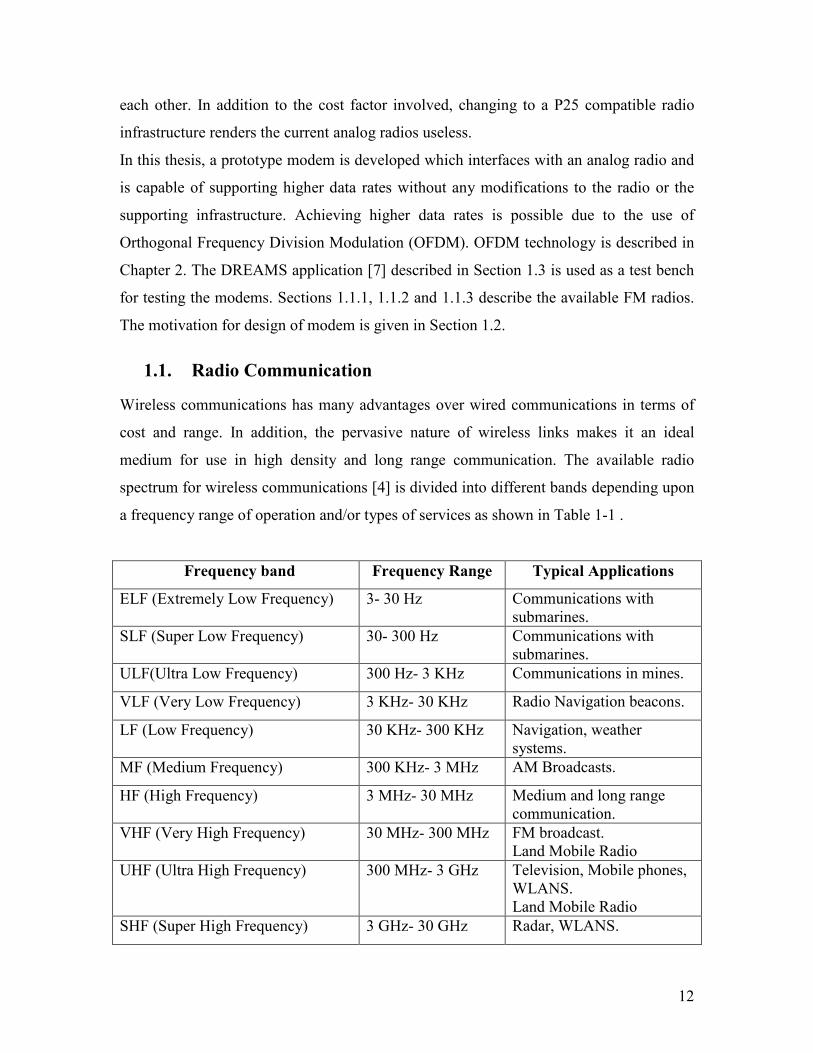
1.1. Radio Communication
Wireless communications has many advantages over wired communications in terms of
cost and range. In addition, the pervasive nature of wireless links makes it an ideal
medium for use in high density and long range communication. The available radio
spectrum for wireless communications [4] is divided into different bands depending upon
a frequency range of operation and/or types of services as shown in Table 1-1 .
Frequency band Frequency Range Typical Applications
ELF (Extremely Low Frequency) 3- 30 Hz Communications with
submarines.
SLF (Super Low Frequency) 30- 300 Hz Communications with
submarines.
ULF(Ultra Low Frequency) 300 Hz- 3 KHz Communications in mines.
VLF (Very Low Frequency) 3 KHz- 30 KHz Radio Navigation beacons.
LF (Low Frequency) 30 KHz- 300 KHz Navigation, weather
systems.
MF (Medium Frequency) 300 KHz- 3 MHz AM Broadcasts.
HF (High Frequency) 3 MHz- 30 MHz Medium and long range
communication.
VHF (Very High Frequency) 30 MHz- 300 MHz FM broadcast.
Land Mobile Radio
UHF (Ultra High Frequency) 300 MHz- 3 GHz Television, Mobile phones,
WLANS.
Land Mobile Radio
SHF (Super High Frequency) 3 GHz- 30 GHz Radar, WLANS.

13
EHF (Extremely High Frequency) 30 GHz- 300 GHz Radio astronomy.
Table 1-1: Frequency Bands.
The UHF and VHF bands are commonly used frequency bands for television. Modern
cell phones technologies like GSM, CDMA also transmit and receive in the UHF band. In
addition to these applications UHF and VHF bands have been traditionally used in land
mobile radio (LMR) applications like public safety organizations, first responders and
amateur radio. These radio applications typically use Amplitude Modulation (AM) and
Frequency modulation (FM) modulation for transmission. AM broadcasts are more
susceptible to noise in the channel as compared to FM which is a constant envelope
modulation. Most of the public radio services currently in service use FM based systems.
1.1.1. Analog Radio
The half duplex radios used in FM communications can be categorized into analog and
digital radios. Analog radio represents the conventional radio systems in which
continuous voice signals are used to frequency modulate the carrier frequency. In the case
of digital radios, a voice signal is mapped into bits depending upon the data modulation
used. The block diagram for an analog radio is given in Figure 1-1. As seen in Figure 1-1,
an analog FM radio contains an audio band pass filter which restricts the frequencies of
the modulating signal, typically between 300 Hz to 3300 Hz. This signal is then fed to a
FM modulator. Chapter 2 introduces the basics of FM modulation while the building
blocks of an FM modulator are given in [1]. Thus, in an analog FM radio a band pass
voice signal frequency modulates the carrier frequency.

14
Figure 1-1: Analog (Half Duplex) FM radio.
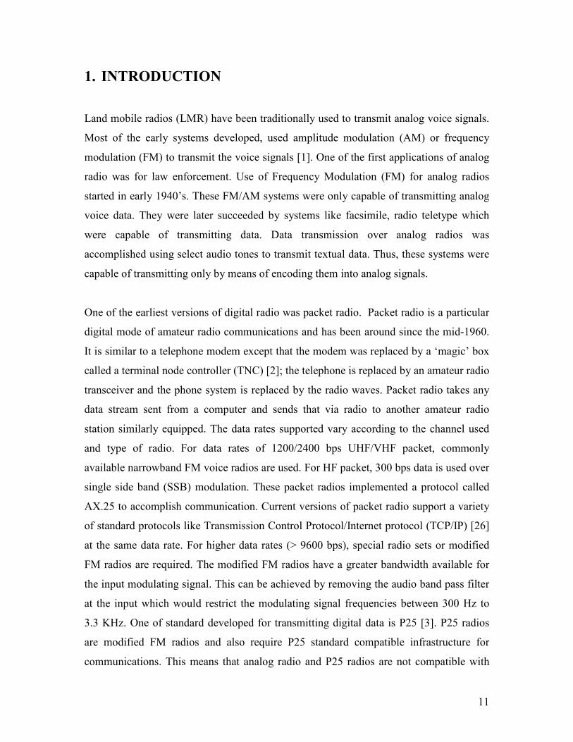
1.1.2. Digital Radio
As opposed to analog radio, a digital FM radio transmits digitized voice as seen in Figure
1-2. The voice is first digitized using an A/D (Analog-to-Digital) converter. This
digitized voice is then passed through a vocoder. The vocoder is a type of speech
coder/decoder which only transmits certain characteristics that represent speech. These
features can be used to reproduce a synthetic equivalent of the input audio. Examples of
popular vocoders are Improved Multi-band Excitation (IMBE), Code Excited Linear
Prediction (CELP) and Advanced Multi-band Excitation (AMBE) [5]. Channel
coding/decoding ensures that the voice data is received correctly by using error detection
and correction codes. In data modulation, the data bits are mapped into channel symbols.
A detailed description of these modules is given in Chapter 3. Such radios are also used
to transmit digital data. An example of a digital radio is the P25 radio. P25 radios support
data rates of 9600 bps. A major drawback of this technology is the requirement for
upgrading the existing infrastructure.
15
Figure 1-2: Digital FM (Half Duplex) radio.
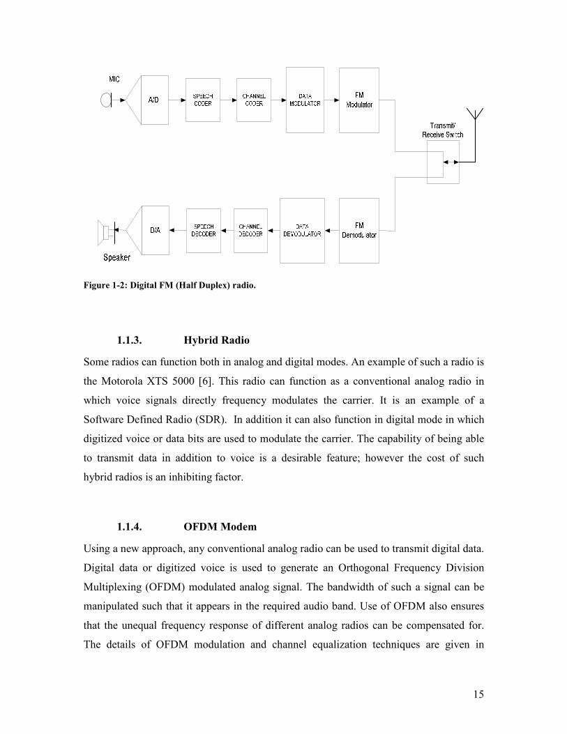
1.1.3. Hybrid Radio
Some radios can function both in analog and digital modes. An example of such a radio is
the Motorola XTS 5000 [6]. This radio can function as a conventional analog radio in
which voice signals directly frequency modulates the carrier. It is an example of a
Software Defined Radio (SDR). In addition it can also function in digital mode in which
digitized voice or data bits are used to modulate the carrier. The capability of being able
to transmit data in addition to voice is a desirable feature; however the cost of such
hybrid radios is an inhibiting factor.
1.1.4. OFDM Modem
Using a new approach, any conventional analog radio can be used to transmit digital data.
Digital data or digitized voice is used to generate an Orthogonal Frequency Division
Multiplexing (OFDM) modulated analog signal. The bandwidth of such a signal can be
manipulated such that it appears in the required audio band. Use of OFDM also ensures
that the unequal frequency response of different analog radios can be compensated for.
The details of OFDM modulation and channel equalization techniques are given in
16
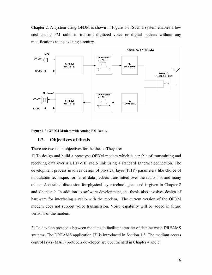
Chapter 2. A system using OFDM is shown in Figure 1-3. Such a system enables a low
cost analog FM radio to transmit digitized voice or digital packets without any
modifications to the existing circuitry.
Figure 1-3: OFDM Modem with Analog FM Radio.
1.2. Objectives of thesis
There are two main objectives for the thesis. They are:
1] To design and build a prototype OFDM modem which is capable of transmitting and
receiving data over a UHF/VHF radio link using a standard Ethernet connection. The
development process involves design of physical layer (PHY) parameters like choice of
modulation technique, format of data packets transmitted over the radio link and many
others. A detailed discussion for physical layer technologies used is given in Chapter 2
and Chapter 9. In addition to software development, the thesis also involves design of
hardware for interfacing a radio with the modem. The current version of the OFDM
modem does not support voice transmission. Voice capability will be added in future
versions of the modem.
2] To develop protocols between modems to facilitate transfer of data between DREAMS
systems. The DREAMS application [7] is introduced in Section 1.3. The medium access
control layer (MAC) protocols developed are documented in Chapter 4 and 5.

17
1.3. DREAMS System
The acronym DREAMS stands for Disaster Remedy and Emergency Medical Services
and is a telemedicine application developed by Texas A&M University and University of
Texas at Huston [7]. It is an advanced telemedicine project designed to speed diagnosis
and treatment of critically injured patients. The project includes designing remote
diagnosis capabilities between a paramedic and physician. The software developed for
the system (which will be referred to as the DREAMS software in this thesis) is capable
of both monitoring and communicating critical and non-critical patient information.
Figure 1-4 and Figure 1-5 show the GUI for the paramedic and physician stations running
the DREAMS software. Both the paramedic station and the physician station are portable
terminals. The paramedic station is equipped with patient health monitoring hardware
like ECG machines, webcam and a defilbulator. In addition to equipment for health
monitoring, a number of communication devices are also connected. The DREAMS
system is capable of establishing a communication link between the paramedic and
physician station using a variety of wireless and wired technologies like cell phones,
satellite radio and Ethernet. The OFDM modem extends these communication
capabilities over VHF/UHF radio links. The paramedic and physician systems work in a
‘client-server’ based architecture. The paramedic station houses the servers for all the
services it provides. The clients are located at the physician terminal. The communication
between the paramedic and physician stations is implemented using the User Datagram
Protocol/ Internet Protocol (UDP/IP) protocol [8]. Each service is identified by the pair of
source and destination port numbers used in UDP protocol. Table 1-2 lists some of the
important services and their respective port numbers. The paramedic station is discussed
in Section 1.3.1 and the physician station is discussed in Section 1.3.2.

18
Port Identifier Type of
information
Port Number
Dreams.port.VitalsPortRange ECG waveform 4100
Dreams.port.NavServerPort GPS co-ordinates 4200
Dreams.port.AudioAllPort Voice signals 4503
Dreams.port.DatabaseServerPort /
dreams.port.DatabaseClient Port
Database contents 4800 / 4801
Dreams.port.VideoServerVideoPort /
dreams.port.VideoClientVideoPort
Video camera
module
4713 / 4715
Dreams.port.TextMessagingServerPort/
dreams.port.TextMessagingClientPort
Text messaging 5200 / 5201
Dreams.port.FileTransferPort/
dreams.port.FileTransferClientPort
File transfer 5300 / 5301
Table 1-2: Services and port numbers.
Figure 1-4:DREAMS: Paramedic station.

19
1.3.1. Paramedic Station
This station is generally housed on the mobile end, for example in an ambulance. The
software on the paramedic station interfaces with a number of medical instruments like
an ECG machine. One of the functions of the software on the paramedic station is to
collect the information from the instruments and relay it to the physician station using
one or more of the available communication media. In addition to critical medical
information, the paramedic station is also capable of transmitting non-critical information
like medical records, patient information, live video and audio streams, video stills and
GPS navigation data. As mentioned in Section 1.3, the paramedic station implements the
servers for the services provided. The GUI for paramedic station is shown in Figure 1-4.
1.3.2. Physician Station
This station can be located in a hospital or a base camp. The GUI for the physician station
is shown in Figure 1-5. The main task of the physician station is to display the
information transmitted by the paramedic station.
Figure 1-5: DREAMS: Physician Station.
20
The physician station also provides a mechanism for a physician to interact with
paramedics using the voice and text messaging capabilities of the DREAMS system.
1.4. Layout of thesis
The first four chapters describe development and design process for a prototype modem.
The second chapter introduces basics of FM transmission and OFDM technology. There
exist a number of ways in which a modem can be built. In the third chapter we describe
the modulator and demodulator structures implemented which use structures well known
in the field digital communications. Thus Chapters 2 and 3 deal with the physical layer
transmission technologies used in the modem. In Chapter 4, the Ethernet interface is
discussed from the perspective of the standard networking Open Systems Interconnection
(OSI) model. The model described in this chapter serves as a platform for the software
implementation of the modem. Chapters 5, 6 and 7 deal exclusively with the design of the
Medium Access Layer (MAC). The design process follows well established norms and
has been modified as per the requirements of the application targeted for demonstrating
the modem.. In Chapter 8, theoretical limits on the performance of the modem under
different conditions have been documented. Improvements and future work is discussed
in Chapter 9.

21
2. INTRODUCTION TO FM AND OFDM
In this chapter we introduce the concepts of frequency modulation (FM), Narrow Band
Frequency Modulation (NBFM) and Orthogonal Frequency Division Multiplexing
(OFDM). Section 1.3 explores the relationship between the bandwidth of the transmitted
signals and the maximum frequency of the modulation signal for a FM signal. The basic
concept of OFDM transmission is explained in Section 2.2. Sections 2.2.1, 2.2.2, 2.2.3,
and 2.2.4 deal with the synchronization and equalization issues associated with OFDM.
2.1. Frequency Modulation
In frequency modulation, the frequency of the carrier is modulated according to the
strength of the modulating signal [1]. Furthermore, the amplitude of the signals remains
constant while the frequency shifts back and forth centered about the center of carrier
frequency. The variation in carrier frequency is a function of the amplitude of the
modulating signal alone. The frequency of the modulating signal determines the rate at
which the frequency changes take place but exerts no influence on the extent of the
changes. The mathematical representation of an FM signal is given by Equation 2-1.
∫+= tccc dmktfAts 0 )(22cos()( ττπ
Equation 2-1
where
M(t) = modulating signal
Ac = carrier amplitude
fc = carrier frequency
if the modulating signal is a sinusoid, given by
)2cos()( tfAtm mm π=
Equation 2-2
where
22
fm = modulating signal frequency
Am = modulating signal amplitude
Then Equation 2-1 reduces to
))2sin(2cos(
))2sin(2cos()(
tftfA
tff
ktfts
mcc
mm
mfA
ccA
πβπ
ππ
+=
+=
Equation 2-3
where
kfAm ( f∆ ) = modulating signal frequency
β ( f∆ /fm) = modulating signal amplitude
Some of the advantages of using frequency modulation are:
1] Constant signal strength.
2] Higher immunity to noise since the modulating signal is recovered from the deviation
of frequency and not the absolute frequency
Some of the disadvantages of frequency modulation will be its sensitivity to phase
distortion and its lower coverage area as compared to amplitude modulation.
2.1.1. Bandwidth Calculation
The frequency bandwidth occupied by the FM signal [9] depends upon two factors:
1) The intensity of the applied modulating signal.
2) The frequency of this modulating signal.
Consider an FM system where the modulating signal is a sinusoid of frequency fm . Upon
the application of the modulating wave the carrier frequency is shifted back and forth
from a maximum position above the carrier frequency to a minimum position below. The
process generates sidebands at frequencies which are multiples of differences and
summations between the modulating signal and the carrier frequency. Theoretically there
is an infinite number of sidebands stretching on both sides of the center frequency.
However, practically, only a finite number of sidebands have sufficient power to be of

23
value towards the reception of the signal. Beyond this, additional sidebands exist but they
carry little or no power and are considered to be unwanted emissions. The intensity of the
modulating signal also affects the distribution of power in the sidebands. The power is
actually drained from the carrier into the sidebands. The stronger the modulating signal,
the greater is the attenuation at the carrier frequency. It is also possible that the strength
of the sidebands is actually greater than that of the carrier frequency. However the total
power of the signal remains constant which is a characteristic of frequency modulation.
As the strength of modulating signal increases the number of significant sidebands
increases as the sidebands that were considered negligible are now accentuated. The
energy spreads out, creating more sidebands of significant power and thereby increasing
the bandwidth of the generated FM signal. It is important to note that the intensity of the
modulating signal only affects the power in the sidebands, not the location of sidebands.
This phenomenon is illustrated in the Figure 2-1.
(a)
(b)
Figure 2-1: Frequency spectrum of FM signal, a) for modulating signal with lower amplitude b) for
modulating signal with higher amplitude.

24
From Figure 2-1 it can be observed that when the modulating signal is weaker, the
resulting FM signal has two significant sideband pairs. If the modulating signal is of
greater strength, then the resulting FM signal has three significant sideband pairs. Thus it
can be concluded that increasing the strength of the modulating signal results in an
increase in the bandwidth of the FM signal transmitted.
The frequency of the modulating signal dictates the locations for the sidebands.
Whenever sidebands are formed they are placed at a distance equal to the frequency of
the modulating signal. For example if the modulating signal is of frequency fm Hz then
the sidebands are created at frequencies given by Equation 2-4.
nfff mci ⋅±= , where n=1, 2….k
Equation 2-4
where,
fi = Frequency of sideband
fm = Maximum modulating frequency
fc = carrier frequency
The spacing of the sidebands also influences the bandwidth calculation for the FM signal
as illustrated in Figure 2-2.
25
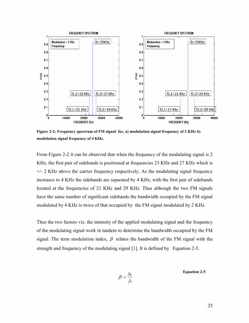
Figure 2-2: Frequency spectrum of FM signal for, a) modulation signal frequency of 2 KHz b)
modulation signal frequency of 4 KHz.
From Figure 2-2 it can be observed that when the frequency of the modulating signal is 2
KHz, the first pair of sidebands is positioned at frequencies 23 KHz and 27 KHz which is
+/- 2 KHz above the carrier frequency respectively. As the modulating signal frequency
increases to 4 KHz the sidebands are separated by 4 KHz, with the first pair of sidebands
located at the frequencies of 21 KHz and 29 KHz. Thus although the two FM signals
have the same number of significant sidebands the bandwidth occupied by the FM signal
modulated by 4 KHz is twice of that occupied by the FM signal modulated by 2 KHz.
Thus the two factors viz. the intensity of the applied modulating signal and the frequency
of the modulating signal work in tandem to determine the bandwidth occupied by the FM
signal. The term modulation index, β relates the bandwidth of the FM signal with the
strength and frequency of the modulating signal [1]. It is defined by Equation 2-5.
m
f
f
∆=β
Equation 2-5

26
where,
f∆ = Deviation (Hz)
fm = Maximum modulating frequency
The higher the value of modulation index,β , the greater is the number of sidebands. The
approximate bandwidth of the FM signal with respect to the modulation index can be
derived using Bessel’s functions and is given in [1]. From the above definition of
modulation index, it is observed that if the frequency of the modulating signal is kept
constant then the bandwidth will depend directly upon the strength of the signal. Also, if
the strength is kept constant then the lower frequencies generate more sidebands. The
Figure 2-3 shows the effects of varying the modulation index on the bandwidth of FM
signal.
Figure 2-3: Frequency spectrum of FM signal.
From Figure 2-3 it is observed that when the modulation index is 0.4 the number of
significant sidebands is 2 and the total bandwidth occupied by the FM signal will be
approximately 4*fm . In case of modulation index 2, the number of significant sidebands
is 8 and the total bandwidth occupied is approximately 8*fm.

27
2.1.2. Transmission Bandwidth of FM signals
As discussed in Section 2.1.1 a FM signal contains infinite number of sidebands resulting
in infinite bandwidth requirement. The strength of the sidebands decreases as we move
away from the carrier frequency. Generally if the amplitude of a sideband is equal or less
than 1 % of the highest spectral component then no noticeable distortion is caused by
band limiting the FM transmission to that sideband frequency. The transmission
bandwidth of a FM signal is the separation between the two frequencies beyond which
none of the sideband frequencies is greater than 1 % of the carrier signal obtained when
the modulation is removed.
In practice, Carson’s rule is used to approximate the bandwidth of the generated FM
signal [10]. Carson’s rule predicts the bandwidth occupied by the significant sidebands of
a FM signal based on the maximum modulation frequency and the corresponding
modulation index. The equation is given by:
)1(2 β+= mfBW
Equation 2-6
where
BW = Bandwidth of FM signal
fm = Maximum modulating frequency
β = Modulation index
2.1.3. FM Broadcast Systems
There are two types of FM broadcast systems viz, Narrow Band Frequency Modulation
(NBFM) and Wide Band Frequency Modulation (WBFM) [9]. They differ in terms of the
maximum permissible deviation of the carrier frequency which in turn dictates the
bandwidth of the transmitted signal. The maximum permissible deviation for NBFM
broadcasts is +/- 2.5 KHz with an adjacent channel spacing of 15, 20 or 25 KHz. The
maximum permissible deviation for WBFM broadcasts is +/- 75 KHz and spacing

28
between adjacent channels is about 200 KHz. NBFM transmissions generally limit the
maximum modulating frequency to about 4 KHz which translates into a modulation index
of 0.625. As compared to NBFM, WBFM has maximum modulating frequency set to 15
KHz. WBFM is used in high fidelity FM broadcasts while NBFM channels are generally
used in public safety systems and by law enforcement agencies.
2.2. Orthogonal Frequency Division Multiplexing (OFDM)
The OFDM technique is used for achieving high data rates and combating multipath
fading in wireless channels [11]. OFDM can be interpreted as a hybrid of multi-carrier
modulation (MCM) and frequency shift keying (FSK) [12]. In MCM the data is sent over
multiple carriers simultaneously. FSK uses a single carrier tone, selected from a set of
orthogonal carriers to transmit the data. During each symbol interval the FSK modulator
sends a pulse of one tone or the other depending upon the information bit to be
transmitted. Equation 2-7 describes the generation of a FSK signal.
otherwise
Tt
TfortfAts ii
,0
22),2exp()(
=
≤≤−
= π
Equation 2-7
where,
si(t) = FSK signal
A = carrier amplitude
fi = Frequency of the sinusoid
T = Symbol Duration
In the case of OFDM modulation, the orthogonal carriers are transmitted simultaneously.
Orthogonality amongst the subcarriers is achieved by ensuring that each subcarrier is
separated by an integer multiple of the inverse of the duration of the OFDM symbol. The
effective bandwidth occupied by the OFDM signal is thus the aggregate of the bandwidth
of the individual subcarriers. The structure of OFDM mitigates the effects of Inter-
symbol Interference (ISI) caused by in a Rayleigh fading environment by spreading the
symbol in time domain.

29
In order to ensure that the subcarrier frequencies do not interfere with each other during
detection, the subcarriers are selected from a set of orthogonal signals. This means that
the spectral peak of each subcarrier overlaps with the spectral nulls of the remaining
carriers. This can be achieved by ensuring that the individual subcarriers are spaced by an
integer multiple of the inverse of the symbol duration. Highest spectral efficiency will be
achieved when the individual carriers/subcarriers are placed precisely one symbol
duration apart. One of the ways to implement OFDM uses the Discrete Fourier Transform
pair (IDFT/DFT) [12]. The implementation of an Inverse Discrete Fourier Transform
(IDFT) which corresponds to OFDM modulation is shown in Figure 2-4;
x n( )1
N0
N 1−
N
X k( ) exp j 2⋅ π⋅ n⋅k
N⋅
⋅∑=
⋅ for 0 n≤ N≤ 0 k≤ N≤,
Figure 2-4: OFDM modulation using IFFT.
A Discrete Fourier Transform (DFT) emulates OFDM demodulation and is given by;
NkNnforN
knjnx
NkX
N
n
≤∑ ≤≤≤−=−
=
1
0
0;0),2exp()(1
)( π
Equation 2-8

30
where
N = Size of DFT
K = Frequency Index
N = Time index
X(k) = Data corresponding to kth subcarrier
X(n) = Time domain signal
The output sequence x(n) is transmitted one symbol at a time across the channels. From
Figure 2-4 it is evident that x(n) represents summation of N individual subcarriers each
modulated by respective data symbols. Prior to the transmission, a cyclic prefix is
appended at the front of the sequence x(n), to obtain an OFDM symbol. This cyclic
prefix, which is also referred to as a guard band [12], is generated from the last m
samples of x(n) and can be expressed as;
pmnformnNxmnx ≤−−+=− )(),()(
Equation 2-9
where
x(n) = Time domain signal
p = Length of cyclic prefix
The length of the cyclic prefix (CP) p is generally selected to be one-fourth of the length
of IDFT output. There are two advantages of using a cyclic prefix. First, appending the
tail portion of IDFT output in front makes the OFDM signal appear periodic with period
N. Secondly; if the length of the cyclic prefix is longer than the channel spread of the
channel then the errors due to ISI will be decreased. Further, the periodicity translates
the linear convolution to circular convolution. Thus the received signal at the
demodulator can be expressed in time and frequency domain as shown in Equation 2-10
and Equation 2-11.
)()()()( nwnhnxnr +⊗=
Equation 2-10
where
31
r(n) = Received Signal
h(n) = Channel Impulse Response
w(n) = Additive white Gaussian noise
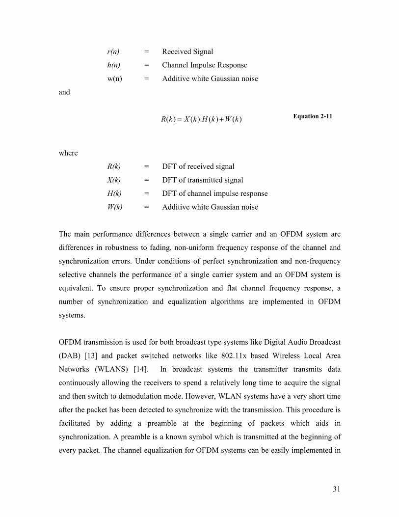
and
)()().()( kWkHkXkR +=
Equation 2-11
where
R(k) = DFT of received signal
X(k) = DFT of transmitted signal
H(k) = DFT of channel impulse response
W(k) = Additive white Gaussian noise
The main performance differences between a single carrier and an OFDM system are
differences in robustness to fading, non-uniform frequency response of the channel and
synchronization errors. Under conditions of perfect synchronization and non-frequency
selective channels the performance of a single carrier system and an OFDM system is
equivalent. To ensure proper synchronization and flat channel frequency response, a
number of synchronization and equalization algorithms are implemented in OFDM
systems.
OFDM transmission is used for both broadcast type systems like Digital Audio Broadcast
(DAB) [13] and packet switched networks like 802.11x based Wireless Local Area
Networks (WLANS) [14]. In broadcast systems the transmitter transmits data
continuously allowing the receivers to spend a relatively long time to acquire the signal
and then switch to demodulation mode. However, WLAN systems have a very short time
after the packet has been detected to synchronize with the transmission. This procedure is
facilitated by adding a preamble at the beginning of packets which aids in
synchronization. A preamble is a known symbol which is transmitted at the beginning of
every packet. The channel equalization for OFDM systems can be easily implemented in

32
frequency domain. Sections 2.2.2 and 2.2.3 describe the synchronization and equalization
structures in detail.
2.2.1. Packet Detection
Timing estimation consists of two parts, viz. packet detection and symbol
synchronization [15]. In the case of broadcast based networks, packet detection is not
required as the transmission is continuous. In packet based networks, which are
essentially random networks, the receiver is constantly monitoring the channel for any
signs of activity. Once a packet is detected the next step is to search for the start of the
data symbols. As mentioned in Section 2.2, a preamble is used in packet oriented
networks which facilitates in the packet detection and symbol synchronization. Packet
detection can be interpreted as coarse estimation and symbol synchronization as a fine
tuning algorithm for detecting the start of signal. In terms of a binary hypothesis test,
packet detection can be interpreted as a choice between two hypotheses;
H0 = Packet not present.
H1 = Packet present.
The simplest method for detecting the start of a packet is to calculate the received signal
energy [16]. The decision variable, mn, used is calculated as shown in Equation 2-12.
∑=−
=−−
1
0
*L
kknknn rrm
Equation 2-12
where,
mn = Decision variable
rn = Received signal
In the absence of actual transmission, the received signal rn consists of noise samples wn
alone. When the actual transmission starts, the received signal is the summation of noise
samples wn and the desired data signal xn. The decision variable, mn, is calculated as a
sum of the squares of the received sample amplitudes over a window of time, L. This

33
represents the energy contained in that window and is referred to as a sliding window.
For iterative computation of the mn the following formula is used;
21
211 +−+− −+= Lnnnn rrmm
Equation 2-13
where,
mn = Decision variable
rn = Received signal
Once the value of decision variable mn exceeds the desired threshold, a valid transmission
is assumed. This method, however, suffers from a significant drawback as the detection
performance depends upon the value of the threshold which is used for the comparison.
The receiver threshold will change dynamically depending upon the received signal
strength. When there is no transmission taking place the received signal consists of noise
alone. The noise level is however unknown and can change if the receiver adjusts the
frontend amplifier settings or in presence of spurious emissions in the frequency band of
interest. Similarly a valid packet transmission also suffers from the irregularity of the
received signal strength. In order to alleviate the degradation in performance due to fixed
thresholding, a double sliding window technique is implemented. In the double sliding
window packet detection algorithm, the received power is calculated over two
consecutive windows. For double window implementation the decision variable mn is
calculated as shown in Equation 2-14.
nnn
L
lnnn
M
mmnmnn
bam
rrb
rra
/
11
*1
1
0
*
=
∑=
∑=
=++
−
=−−
Equation 2-14
where
an = Energy in window A
bn = Energy in window B
rn = Received Signal
34
mn = Decision variable
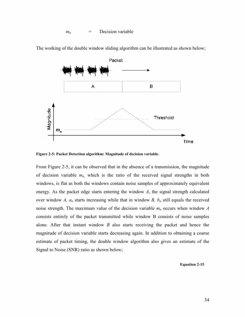
The working of the double window sliding algorithm can be illustrated as shown below;
Figure 2-5: Packet Detection algorithm: Magnitude of decision variable.
From Figure 2-5, it can be observed that in the absence of a transmission, the magnitude
of decision variable mn, which is the ratio of the received signal strengths in both
windows, is flat as both the windows contain noise samples of approximately equivalent
energy. As the packet edge starts entering the window A, the signal strength calculated
over window A, an starts increasing while that in window B, bn still equals the received
noise strength. The maximum value of the decision variable mn occurs when window A
consists entirely of the packet transmitted while window B consists of noise samples
alone. After that instant window B also starts receiving the packet and hence the
magnitude of decision variable starts decreasing again. In addition to obtaining a coarse
estimate of packet timing, the double window algorithm also gives an estimate of the
Signal to Noise (SNR) ratio as shown below;
Equation 2-15
35
1
1min
max
−=
+=+
==
peak
n
npeak
mN
S
N
S
N
NS
ba
m
where,
mpeak = Maximum value of decision variable
an = Maximum energy content from window A
bn = Minimum energy content from window B
S/N = Signal to Noise ratio of the received signal
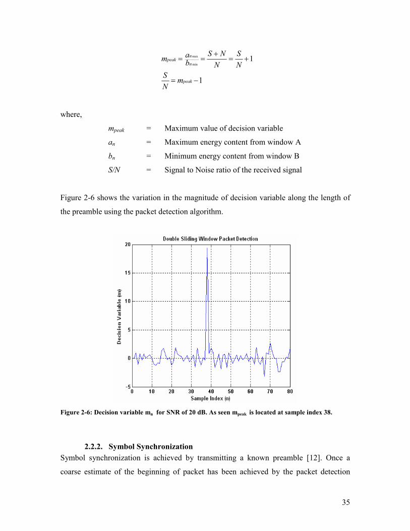
Figure 2-6 shows the variation in the magnitude of decision variable along the length of
the preamble using the packet detection algorithm.
Figure 2-6: Decision variable mn for SNR of 20 dB. As seen mpeak is located at sample index 38.
2.2.2. Symbol Synchronization
Symbol synchronization is achieved by transmitting a known preamble [12]. Once a
coarse estimate of the beginning of packet has been achieved by the packet detection
36
algorithm, a simple correlation based approach can be used to fine tune the start of
transmission. The fine tuning is achieved by calculating the cross correlation between the
received signal, r(t) and the known reference template, s(t).
The sample index which corresponds to the maximum correlation is selected as the likely
start of transmission. The accuracy of the correlation algorithm depends upon the length
over which correlation is performed. However, there is a tradeoff between the length of
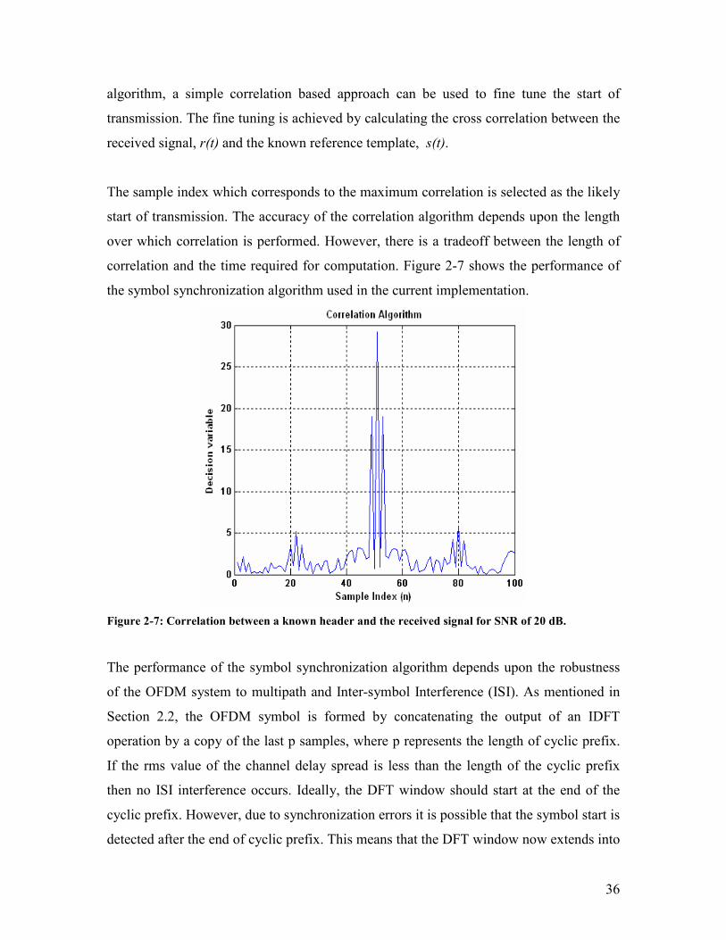
correlation and the time required for computation. Figure 2-7 shows the performance of
the symbol synchronization algorithm used in the current implementation.
Figure 2-7: Correlation between a known header and the received signal for SNR of 20 dB.
The performance of the symbol synchronization algorithm depends upon the robustness
of the OFDM system to multipath and Inter-symbol Interference (ISI). As mentioned in
Section 2.2, the OFDM symbol is formed by concatenating the output of an IDFT
operation by a copy of the last p samples, where p represents the length of cyclic prefix.
If the rms value of the channel delay spread is less than the length of the cyclic prefix
then no ISI interference occurs. Ideally, the DFT window should start at the end of the
cyclic prefix. However, due to synchronization errors it is possible that the symbol start is
detected after the end of cyclic prefix. This means that the DFT window now extends into

37
the ensuing OFDM symbol resulting in ISI. In order to ensure that no ISI takes place, the
start of symbol is biased such that it always points to a sample inside the cyclic prefix of
that OFDM symbol. Since the cyclic prefix is composed of the last p samples, the
frequency content of the OFDM symbol is preserved, only the time domain data changes.
Figure 2-8 below shows the operation of symbol synchronization;
Figure 2-8: Ideal Synchronization for packet header.
In Figure 2-8 we have three contiguous OFDM symbols. As mentioned above, the ideal
DFT window for symbol#2 would be at the end of the cyclic prefix, CP#2. However, if
the DFT window extends into the cyclic prefix of symbol#3, then the demodulated data
will be corrupted. In Figure 2-8 we observe that the start of symbol is biased such that it
lies within the cyclic prefix CP#2. Thus, it is ensured that the DFT window for symbol#2
will lie within the symbol boundary.
2.2.3. Equalization
The structure of OFDM allows high spectral efficiency by transmitting data in parallel
streams. Mobile radio channels, however, are affected by multipath fading, which results

38
in degraded radio performance. In OFDM, the number of subcarriers is chosen such that
the channel frequency response is essentially flat over each subcarrier, thus reducing the
effect of fading and non-uniform channel frequency response. Combining channel coding
and OFDM permits reliable data transmission over dispersive channels. In order to
compensate for multipath fading and channel frequency response, various channel
equalization techniques are used. Equalization techniques can be implemented in the time
domain and/or the frequency domain [17] [18]. Many adaptive equalization algorithms
are used to compensate for multipath in the frequency domain. Commonly used
algorithms include decision feedback equalization (DFE) and Least-Mean-Squares
(LMS) equalization. Channel equalization in the frequency domain can be performed
using two main approaches. The first approach uses training data transmitted on every
subcarrier at the beginning of each transmitted packet. This technique, which is widely
used in WLAN systems, is referred as a block-type pilot structure. The second approach
uses a comb-type pilot arrangement and involves inserting pilot subcarriers into OFDM
symbols at a suitable spacing. The frequency response for the entire channel is then
interpolated from the channel response obtained at pilot sub-carriers. Section 2.2.4
discusses frequency domain adaptable equalization algorithm which uses a block type
pilot structure.
2.2.4. Frequency domain Adaptive Equalization methods
From Equation 2-11, we observe that the received signal is given by
)()()()( kWkHkXkR +=
Equation 2-16
where
R(k) = DFT of received signal
X(k) = DFT of transmitted signal
H(k) = DFT of channel impulse response
W(k) = Additive white gaussian noise

39
Let the estimated channel response be denoted by C(k) such that the equalized data
sample )(kX is given by
)()()()()()()()( kCkWkCkHkXkCkRkX +==
Equation 2-17
where
)(kX = Equalized data sample
X(k) = DFT of transmitted signal
H(k) = DFT of channel impulse response
W(k) = Additive white gaussian noise
C(k) = Estimated channel response
Now if the estimated channel response C(k) is C(k)= H-1(k) then, in absence of noise, the
equalized sample will equate to )()()()()( kXkCkHkXkX == [19].
As discussed in Section 2.2.3, in the block-type pilot arrangement used in many packet
switched networks, the initial estimate of the channel response is obtained from the
training data. This initial estimate can now be used to equalize the received data samples.
Thus the error in estimation of the received symbols will be given by Equation 2-18 [33]:
∏−−
−= )),((),(),( kjXkjXkjε
Equation 2-18
where
),( kjε = Error between the jth carrier of k
th symbol
∏ (.) is the threshold operator which maps the estimated sample to a valid data value.
The error in estimation depends on the noise W(k).
40
The simplest implementation for an equalizer structure uses the Least Squares (LS)
algorithm [20]. The LS estimate which minimizes the error is given by Equation 2-19.
)()()( 1 kRkXkC −=
Equation 2-19
In presence of slow fading, we can use the decision feedback equalizer (DFE) structure to
update the channel coefficients associated with each subcarrier. The decision feedback
equalizer for the kth subcarrier is given by the following equation,
1,,0
)),((
)()( −=
∏
=−
Nfork
kjX
kRkC …
Equation 2-20
The performance of the DFE depends upon the correctness of the mapped symbols and
hence is prone to errors in fast fading environments. Another possible approach for the
equalizer structure is Minimum Mean Square error (MMSE) [19]. From Equation 2-18
we can observe that the error can be reduced by using the mean squared error as the cost
function [33].
),(),(2),( * kjRkj
C
kjε
ε=
∂
∂
Equation 2-21
The channel response coefficients are updated by the addition of a weighted error term
[33].
),1(),1(2),1(),( * kjRkjkjCkjC −−+−= µε
Equation 2-22
where C(j,k) is the channel response corresponding to the kth subcarrier at j
th time instant
and ]1,0[∈µ represents the learning constant. This algorithm however has a higher
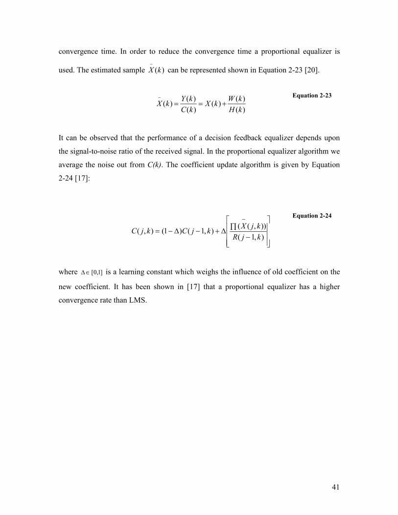
41
convergence time. In order to reduce the convergence time a proportional equalizer is
used. The estimated sample )(kX−
can be represented shown in Equation 2-23 [20].
)(
)()(
)(
)()(
kH
kWkX
kC
kYkX +==
−
Equation 2-23
It can be observed that the performance of a decision feedback equalizer depends upon
the signal-to-noise ratio of the received signal. In the proportional equalizer algorithm we
average the noise out from C(k). The coefficient update algorithm is given by Equation
2-24 [17]:
−∏∆+−∆−=
−
),1(
)),((),1()1(),(
kjR
kjXkjCkjC
Equation 2-24
where ]1,0[∈∆ is a learning constant which weighs the influence of old coefficient on the
new coefficient. It has been shown in [17] that a proportional equalizer has a higher
convergence rate than LMS.
42
3. MODEM DESIGN
The term Modem stands for Modulator/Demodulator and can be defined as a
communications device which converts a signal from one form to another for
transmission over a communication channel [10]. Historically, modems have been
associated with telephony where the primary function of the device was to convert digital
signals into analog signals for transmission over the telephone lines. Nowadays, modems
are used over cable connections, satellite links, land mobile radios, etc. This Chapter
introduces the different aspects of OFDM modem design and includes a detailed
discussion on the various modules used in the modulation and demodulation of a data
signal.
The OFDM modem design can be demarcated into two parts. The first part deals with the
modules which make up the modulator and demodulator. As mentioned in Chapter 1, the
OFDM modem should be capable of communicating using standard Ethernet protocols
and with an analog radio. The current modem hardware consists of a NetBurner® card, a
Motorola 56L307® evaluation module (EVM) DSP evaluation board and a customized
daughter card. The NetBurner® card houses the Ethernet stack while the daughter card is
used to provide an interface between the radio and the modem. The EVM is used to
implement the signal processing associated with modulation and demodulation. Sections
3.1 and 3.2 describe the implementation of the modulator and demodulator in the EVM.
The second part of the modem design deals with the system architecture which will be
discussed in Chapter 4.
3.1. Modulator Block Diagram
The function of the modulator is to process the raw data received over a serial port from
the NetBurner into a signal compatible with the radio used. The modulator block diagram
can be partitioned into three distinct modules. The first part involves scrambling
operation followed by convolutional coding and interleaving. The second part includes
the generation of OFDM symbols at the baseband frequency. In the final phase the
43
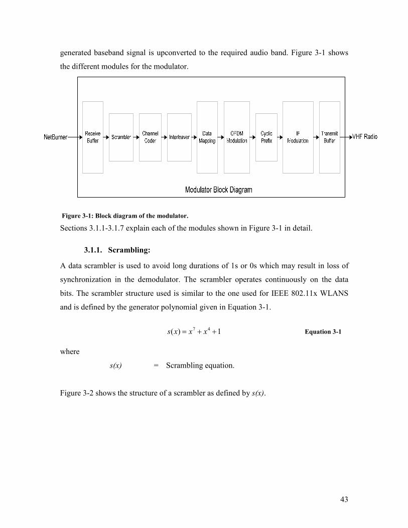
generated baseband signal is upconverted to the required audio band. Figure 3-1 shows
the different modules for the modulator.
Figure 3-1: Block diagram of the modulator.
Sections 3.1.1-3.1.7 explain each of the modules shown in Figure 3-1 in detail.
3.1.1. Scrambling:
A data scrambler is used to avoid long durations of 1s or 0s which may result in loss of
synchronization in the demodulator. The scrambler operates continuously on the data
bits. The scrambler structure used is similar to the one used for IEEE 802.11x WLANS
and is defined by the generator polynomial given in Equation 3-1.
1)( 47 ++= xxxs
Equation 3-1
where
s(x) = Scrambling equation.
Figure 3-2 shows the structure of a scrambler as defined by s(x).

44
Figure 3-2 : Block diagram for scrambler.
The operation of the scrambler can be compared to that of a linear feedback shift register.
The individual bits enter the shift register and get permuted based on the scrambing
equation. The output bit for the scrambler is given by the expression in Equation 3-2.
74 xxDataInDataOut ⊕⊕=
Equation 3-2
3.1.2. Channel Coder
Channel coding is used to improve the performance of the system in the presence of
noisy and fading environments [21]. Reliability is obtained by selective addition of
redundant bits into the transmitted information signal. The added bits can be used for
both detection and correction of errors. However the increased reliability comes at the
expense of a reduction in the data rate. There are two main classes of channel codes viz;
Block codes and Convolutional codes. Block codes are based on finite field arithmetic
and abstract algebra and can be used in both detection and correction of errors, which
occur during transmission. Block codes accept a block of k information bits as input and
produce a block of n coded bits. Some of the commonly used block codes are Hamming
codes, Golay Codes, BCH codes and Reed Solomon codes.
The most widely used channel codes are convolutional codes. The codes are developed
for real-time error detection and correction. The convolutional codes convert the entire
data stream into code words. The encoded data not only depends on the current input but
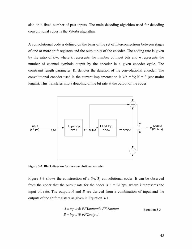
45
also on a fixed number of past inputs. The main decoding algorithm used for decoding
convolutional codes is the Viterbi algorithm.
A convolutional code is defined on the basis of the set of interconnections between stages
of one or more shift registers and the output bits of the encoder. The coding rate is given
by the ratio of k/n, where k represents the number of input bits and n represents the
number of channel symbols output by the encoder in a given encoder cycle. The
constraint length parameter, K, denotes the duration of the convolutional encoder. The
convolutional encoder used in the current implementation is k/n = ½; K = 3 (constraint
length). This translates into a doubling of the bit rate at the output of the coder.
Figure 3-3: Block diagram for the convolutional encoder
Figure 3-3 shows the construction of a (½, 3) convolutional coder. It can be observed
from the coder that the output rate for the coder is n = 2k bps, where k represents the
input bit rate. The outputs A and B are derived from a combination of input and the
outputs of the shift registers as given in Equation 3-3.
outputFFinputB
outputFFoutputFFinputA
2
21
⊕=
⊕⊕=
Equation 3-3

46
where,
A = Output#1
B = Output#2
FF1output = Output for Flip flopFF#1
FF2output = Output for Flip flop FF#2
For example suppose that the input data stream is 10101. Let the initialization state for
the coder be the reset state. The code words corresponding to the input will be as shown
in Table 3-1.
Input FF#1output FF#2output Output A
input FF1output⊕ FF2output⊕
Output B
input FF2output⊕
1 0 0 1 1
0 1 0 1 0
1 0 1 0 0
0 1 0 1 0
1 0 1 0 0
Table 3-1: Output of a (1/2, 3) convolutional encoder
The output of the channel coder will be 1110001000. Thus the output bit rate n is twice
the input bit rate k.
3.1.3. Interleaver
Interleaving is used to distribute the coded bits in time, frequency or both to mitigate the
degradation in performance caused due to burst errors [12]. The type of interleaving
pattern used depends upon the channel characteristics. If the system operates in an
AWGN environment alone, then rearranging adjacent bits does not improve the Bit Error
Rate (BER). However errors caused due to fading and random bursts of noise can be
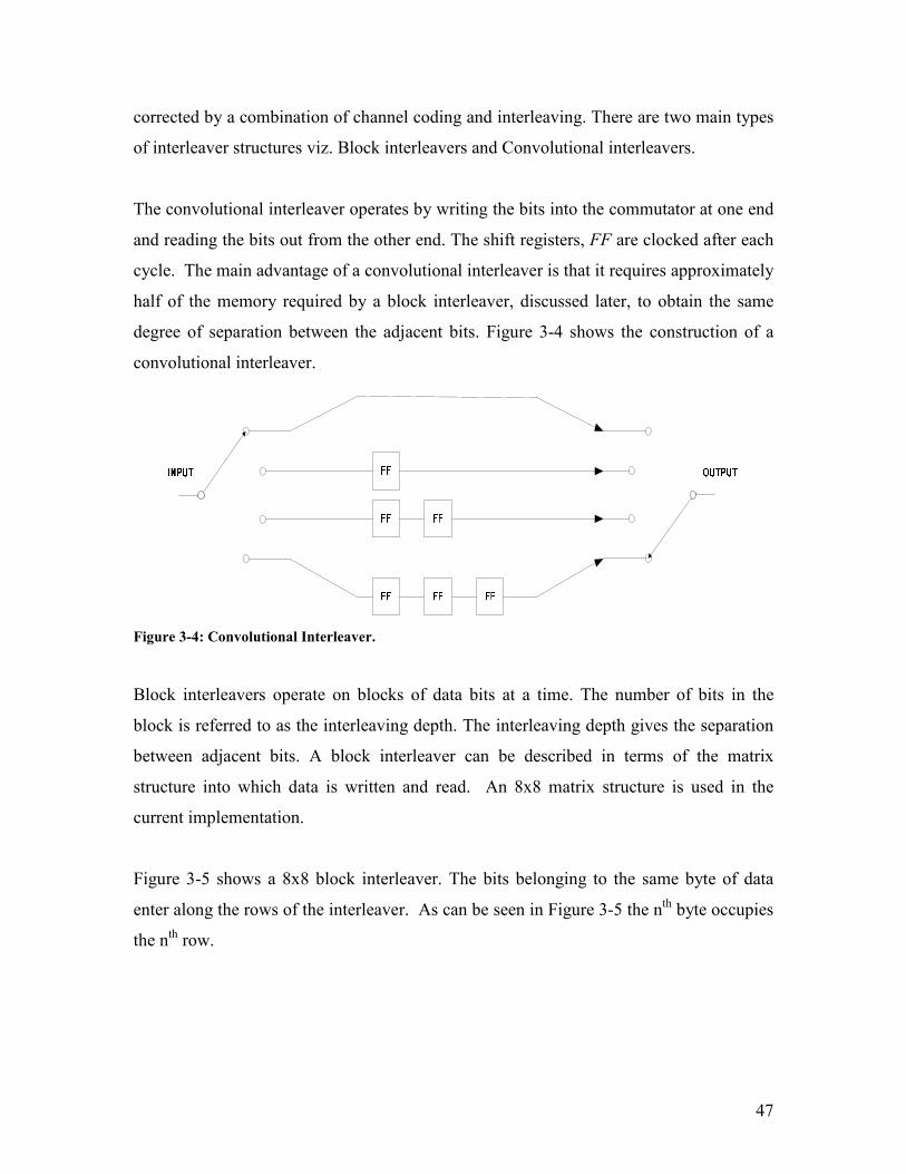
47
corrected by a combination of channel coding and interleaving. There are two main types
of interleaver structures viz. Block interleavers and Convolutional interleavers.
The convolutional interleaver operates by writing the bits into the commutator at one end
and reading the bits out from the other end. The shift registers, FF are clocked after each
cycle. The main advantage of a convolutional interleaver is that it requires approximately
half of the memory required by a block interleaver, discussed later, to obtain the same
degree of separation between the adjacent bits. Figure 3-4 shows the construction of a
convolutional interleaver.
Figure 3-4: Convolutional Interleaver.
Block interleavers operate on blocks of data bits at a time. The number of bits in the
block is referred to as the interleaving depth. The interleaving depth gives the separation
between adjacent bits. A block interleaver can be described in terms of the matrix
structure into which data is written and read. An 8x8 matrix structure is used in the
current implementation.
Figure 3-5 shows a 8x8 block interleaver. The bits belonging to the same byte of data
enter along the rows of the interleaver. As can be seen in Figure 3-5 the nth byte occupies
the nth row.
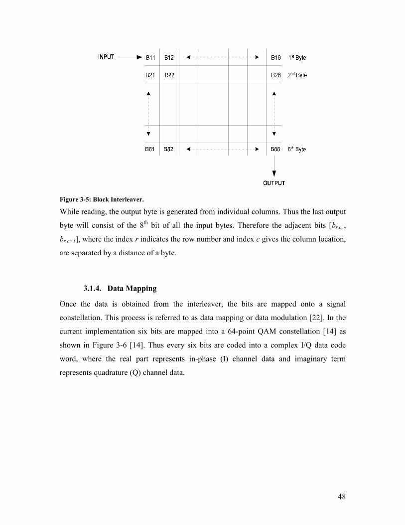
48
Figure 3-5: Block Interleaver.
While reading, the output byte is generated from individual columns. Thus the last output
byte will consist of the 8th bit of all the input bytes. Therefore the adjacent bits [br,c ,
br,c+1], where the index r indicates the row number and index c gives the column location,
are separated by a distance of a byte.
3.1.4. Data Mapping
Once the data is obtained from the interleaver, the bits are mapped onto a signal
constellation. This process is referred to as data mapping or data modulation [22]. In the
current implementation six bits are mapped into a 64-point QAM constellation [14] as
shown in Figure 3-6 [14]. Thus every six bits are coded into a complex I/Q data code
word, where the real part represents in-phase (I) channel data and imaginary term
represents quadrature (Q) channel data.

49
Figure 3-6: Constellation diagram for 64 QAM
3.1.5. OFDM Modulation
As discussed in Chapter 2, OFDM modulation is performed by applying the Inverse Fast
Fourier Transform (IFFT) operation on the constellation mapped complex data set. The
size of the IFFT used gives the maximum number of subcarriers that can be used to
transmit data. The IFFT operation is given by the Equation 3-4.
NkNnforN
knjnx
NkX
N
n
≤∑ ≤≤≤=−
=
1
0
0;0),2exp()(1
)( π
Equation 3-4
where
N = Size of DFT
K = Frequency Index
N = Time index
X(k) = Data corresponding to kth subcarrier
x(n) = Time domain signal
In the current implementation, the size of the IFFT used is 64. The combined bandwidth
of all the subcarriers in the OFDM symbol is 1 KHz. The time domain and frequency
domain signal characteristics will be explored in Chapter 8.

50
3.1.6. Cyclic Prefix
After OFDM modulation, a cyclic prefix is appended at the beginning to form an OFDM
symbol. The advantages of incorporating a cyclic prefix have been discussed in Chapter
2. The length of cyclic prefix selected for the current implementation is 16, which is one
fourth the length of the IFFT.
3.1.7. Upconversion
The baseband OFDM symbol is a complex signal with the real part corresponding to I
channel data and the imaginary part corresponding to the Q channel data. The need for
upconversion arises due the frequency response of the radio which is designed for the
transmission of voice signals. The frequency response of the radio can be equated
roughly to that of a bandpass filter with cut off frequencies at 300 Hz and 3.3 KHz. In
order to ensure that no information is lost, the baseband OFDM symbol has to be
upconverted to a suitable passband. The Figure 3-7 represents the approximate magnitude
of the complex baseband OFDM signal.
Figure 3-7: Frequency spectrum for baseband OFDM symbol.
The choice of audio band carrier frequency used for upconversion depends on the
sampling rate of the codec, the frequency response of the radio used and the bandwidth of
the baseband signal.
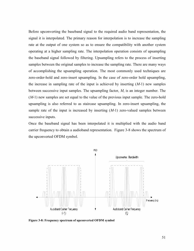
51
Before upconverting the baseband signal to the required audio band representation, the
signal it is interpolated. The primary reason for interpolation is to increase the sampling
rate at the output of one system so as to ensure the compatibility with another system
operating at a higher sampling rate. The interpolation operation consists of upsampling
the baseband signal followed by filtering. Upsampling refers to the process of inserting
samples between the original samples to increase the sampling rate. There are many ways
of accomplishing the upsampling operation. The most commonly used techniques are
zero-order-hold and zero-insert upsampling. In the case of zero-order hold upsampling,
the increase in sampling rate of the input is achieved by inserting (M-1) new samples
between successive input samples. The upsampling factor, M, is an integer number. The
(M-1) new samples are set equal to the value of the previous input sample. The zero-hold
upsampling is also referred to as staircase upsampling. In zero-insert upsampling, the
sample rate of the input is increased by inserting (M-1) zero-valued samples between
successive inputs.
Once the baseband signal has been interpolated it is multiplied with the audio band
carrier frequency to obtain a audioband representation. Figure 3-8 shows the spectrum of
the upconverted OFDM symbol.
Figure 3-8: Frequency spectrum of upconverted OFDM symbol

52
As mentioned in Sections 3.1.5 and 3.1.6, for the current implementation the total number
of samples representing a single baseband OFDM symbol is 80 samples. Also, in the
current implementation, the interpolation operation consists of zero-insert upsampling
followed by FIR filtering [23]. The interpolation factor is 4 and the length of FIR filter is
24. For the codec sampling rate of 8 KHz and audio band carrier frequency of 2 KHz the
spectrum of the baseband OFDM symbol and upconverted OFDM symbol are given in
Figure 3-9 and Figure 3-10 respectively. Further details on the calculation of bandwidths
and data rates are given in Chapter 7.
Figure 3-9: Baseband OFDM frequency spectrum generated using sampling rate of 8 Khz.
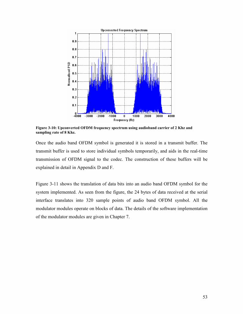
53
Figure 3-10: Upconverted OFDM frequency spectrum using audioband carrier of 2 Khz and
sampling rate of 8 Khz.
Once the audio band OFDM symbol is generated it is stored in a transmit buffer. The
transmit buffer is used to store individual symbols temporarily, and aids in the real-time
transmission of OFDM signal to the codec. The construction of these buffers will be
explained in detail in Appendix D and F.
Figure 3-11 shows the translation of data bits into an audio band OFDM symbol for the
system implemented. As seen from the figure, the 24 bytes of data received at the serial
interface translates into 320 sample points of audio band OFDM symbol. All the
modulator modules operate on blocks of data. The details of the software implementation
of the modulator modules are given in Chapter 7.

54
Figure 3-11: Translation of individual data bits to OFDM symbols.
3.2. Demodulator Block Diagram
The function of the demodulator is to process the received signal at the radio into raw
data bits and transmit these bits over the serial port to the NetBurner. The demodulator
block diagram can also be partitioned into three distinct modules. The first part involves
demodulation of the received audio band OFDM signal into its baseband representation.
The second part includes demodulation of the baseband OFDM symbols and demapping
the complex symbols into their corresponding bit representation. In the final phase, the
bits are deinterleaved, decoded and descrambled to obtain raw data bits to be transmitted
over the serial port to the NetBurner card.
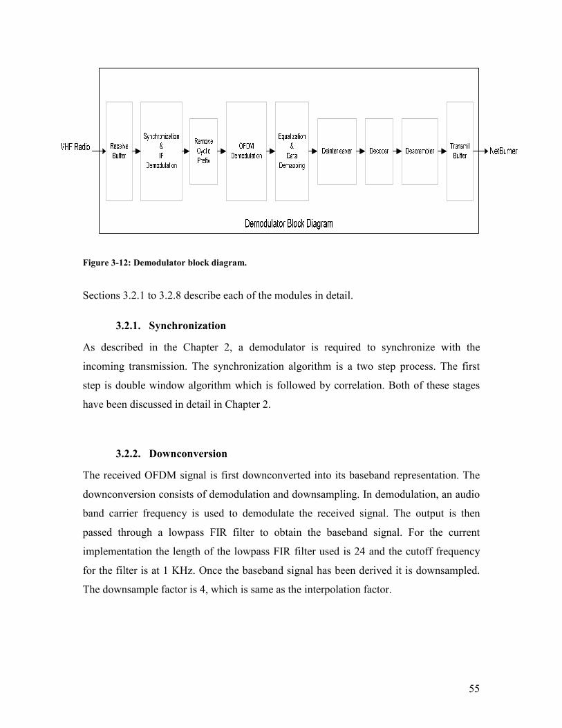
55
Figure 3-12: Demodulator block diagram.
Sections 3.2.1 to 3.2.8 describe each of the modules in detail.
3.2.1. Synchronization
As described in the Chapter 2, a demodulator is required to synchronize with the
incoming transmission. The synchronization algorithm is a two step process. The first
step is double window algorithm which is followed by correlation. Both of these stages
have been discussed in detail in Chapter 2.
3.2.2. Downconversion
The received OFDM signal is first downconverted into its baseband representation. The
downconversion consists of demodulation and downsampling. In demodulation, an audio
band carrier frequency is used to demodulate the received signal. The output is then
passed through a lowpass FIR filter to obtain the baseband signal. For the current
implementation the length of the lowpass FIR filter used is 24 and the cutoff frequency
for the filter is at 1 KHz. Once the baseband signal has been derived it is downsampled.
The downsample factor is 4, which is same as the interpolation factor.
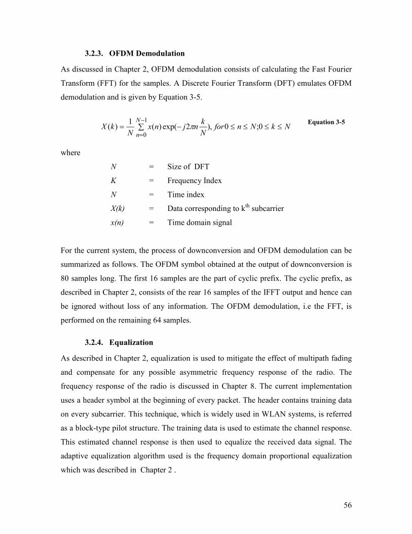
56
3.2.3. OFDM Demodulation
As discussed in Chapter 2, OFDM demodulation consists of calculating the Fast Fourier
Transform (FFT) for the samples. A Discrete Fourier Transform (DFT) emulates OFDM
demodulation and is given by Equation 3-5.
NkNnforN
knjnx
NkX
N
n
≤∑ ≤≤≤−=−
=
1
0
0;0),2exp()(1
)( π
Equation 3-5
where
N = Size of DFT
K = Frequency Index
N = Time index
X(k) = Data corresponding to kth subcarrier
x(n) = Time domain signal
For the current system, the process of downconversion and OFDM demodulation can be
summarized as follows. The OFDM symbol obtained at the output of downconversion is
80 samples long. The first 16 samples are the part of cyclic prefix. The cyclic prefix, as
described in Chapter 2, consists of the rear 16 samples of the IFFT output and hence can
be ignored without loss of any information. The OFDM demodulation, i.e the FFT, is
performed on the remaining 64 samples.
3.2.4. Equalization
As described in Chapter 2, equalization is used to mitigate the effect of multipath fading
and compensate for any possible asymmetric frequency response of the radio. The
frequency response of the radio is discussed in Chapter 8. The current implementation
uses a header symbol at the beginning of every packet. The header contains training data
on every subcarrier. This technique, which is widely used in WLAN systems, is referred
as a block-type pilot structure. The training data is used to estimate the channel response.
This estimated channel response is then used to equalize the received data signal. The
adaptive equalization algorithm used is the frequency domain proportional equalization
which was described in Chapter 2 .

57
3.2.5. Data Demapping
In this module the output of the FFT is mapped into data bits using the signal
constellation which was described in Section 3.1.4. The complex values obtained at the
output of the FFT module represent the in-phase (I) and quadrature (Q) phase
components. The corresponding point in the signal constellation is used to obtain the
demapped bits. The demapping process involves comparing the received symbol with
decision thresholds. The decision thresholds were selected on the basis of maximum
likelihood estimation. Since the current design uses 64-QAM data mapping, the 64
samples obtained at the end of OFDM demodulation transform into 48 bytes at the end of
this module.
3.2.6. Deinterleaving
The structure of the deinterleaver is similar to that of the interleaver. The same 8x8
matrix structure, discussed in Section 3.1.3, used in interleaving is used to realign the
adjacent bits.
3.2.7. Decoder
There are two main decoding algorithms which are used with convolutional encoding.
They are sequential decoding and Viterbi decoding. Sequential decoding is better suited
for convolutional codes with longer constraint length. However this type of decoding has
variable decoding time. In the current implementation the Viterbi algorithm has been
used to decode the bits. The Viterbi decoder is a maximum likelihood (ML) decoding
procedure for convolutional codes. Further there are two ways to implement Viterbi
algorithm viz. hard decision and soft decision. The current implementation uses Viterbi
decoder in hard decision format. For more details about the operation of a Viterbi
decoder, refer to [24]. As mentioned in Section 3.1.2, the channel coder used in the
current implementation is (1/2, 3). Thus, the output of the decoder will have half the
number of bits as the input which is 24 bytes in the current system.
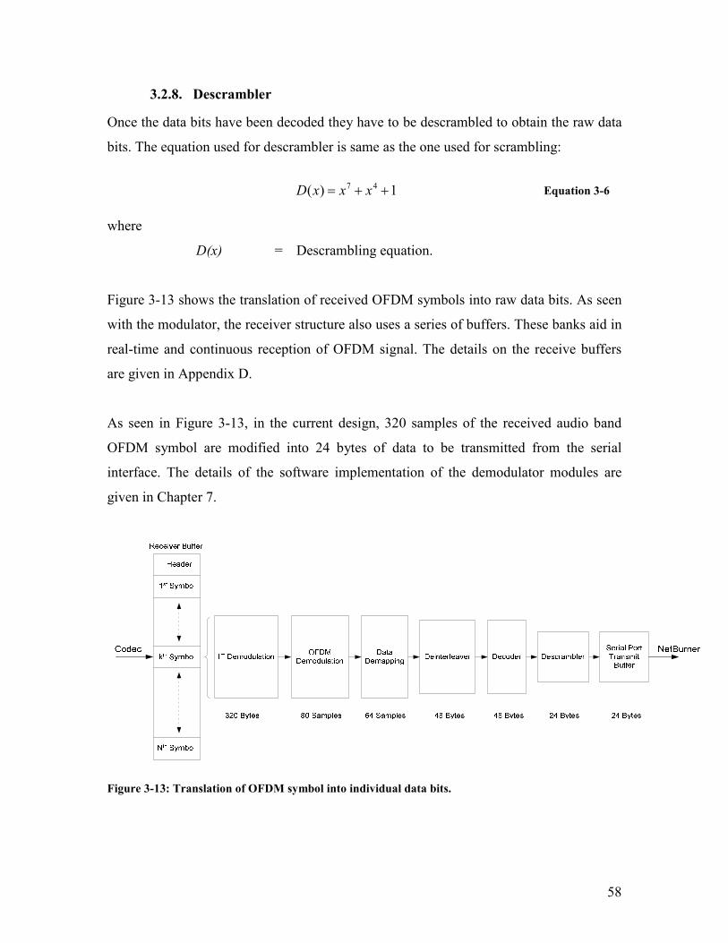
58
3.2.8. Descrambler
Once the data bits have been decoded they have to be descrambled to obtain the raw data
bits. The equation used for descrambler is same as the one used for scrambling:
1)( 47 ++= xxxD
Equation 3-6
where
D(x) = Descrambling equation.
Figure 3-13 shows the translation of received OFDM symbols into raw data bits. As seen
with the modulator, the receiver structure also uses a series of buffers. These banks aid in
real-time and continuous reception of OFDM signal. The details on the receive buffers
are given in Appendix D.
As seen in Figure 3-13, in the current design, 320 samples of the received audio band
OFDM symbol are modified into 24 bytes of data to be transmitted from the serial
interface. The details of the software implementation of the demodulator modules are
given in Chapter 7.
Figure 3-13: Translation of OFDM symbol into individual data bits.
59
4. SYSTEM ARCHITECTURE
As described in Chapter 3, the modem design can be demarcated into two parts. The first
part deals with the modular construction of the modem while the second part deals with
its system design. System design refers to the interfaces of the modem and the signal
processing and packaging of the data bits. Section 4.1 gives an overview of the system
architecture. In Section 4.3 the implementation of the physical layer has been discussed.
In addition to the ability to modulate and demodulate data, the modem has to perform a
number of functions, like access control, which ensure harmonious operation between the
interfaced devices. Such issues have been discussed in Section 4.3.1.
4.1. System Overview
Figure 4-1 depicts a typical configuration of a system in which the modems are used. As
shown in the figure, Data Terminal Equipment (DTE) 1 is interfaced with Modem 1 via
an RJ-45 connection. Modem 1 is, in turn, connected to a radio [25]. Similarly Data
Terminal Equipment (DTE) 2 is interfaced with Modem 2 which is also connected to a
radio. The communication between the terminal and the modem is carried out using
Ethernet packets. The communication is directed between the modem and the terminal
interfaced with it using the IP addresses of the respective entities. That is to say that all
the packets, which are to be transmitted by the terminal, are sent to the IP address of the
modem and similarly, all the packets which are received by the modem are sent to the IP
address of the connected terminal. The purpose of this setup is to ensure that the
applications are not required to keep a track of the IP addresses of other terminals in the
system. There are two ways of assigning IP addresses. One approach is to code the IP
address into the modems. This is referred to as static IP allocation. Another approach,
which is more flexible, is to dynamically assign IP addresses using the Dynamic Host
Routing Protocol (DHCP). For dynamic IP assignment to work, the terminal interfaced
with the modem must exhibit DHCP capabilities. The modems communicate with each
other using radios. Although Figure 4-1 shows a configuration with two modems having
a single bidirectional radio link, the design concept is also applicable to multi-modem
environments.
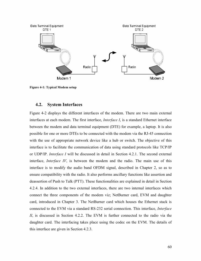
60
Figure 4-1: Typical Modem setup
4.2. System Interfaces
Figure 4-2 displays the different interfaces of the modem. There are two main external
interfaces at each modem. The first interface, Interface I, is a standard Ethernet interface
between the modem and data terminal equipment (DTE) for example, a laptop. It is also
possible for one or more DTEs to be connected with the modem via the RJ-45 connection
with the use of appropriate network device like a hub or switch. The objective of this
interface is to facilitate the communication of data using standard protocols like TCP/IP
or UDP/IP. Interface I will be discussed in detail in Section 4.2.1. The second external
interface, Interface IV, is between the modem and the radio. The main use of this
interface is to modify the audio band OFDM signal, described in Chapter 2, so as to
ensure compatibility with the radio. It also performs ancillary functions like assertion and
deassertion of Push to Talk (PTT). These functionalities are explained in detail in Section
4.2.4. In addition to the two external interfaces, there are two internal interfaces which
connect the three components of the modem viz; NetBurner card, EVM and daughter
card, introduced in Chapter 3. The NetBurner card which houses the Ethernet stack is
connected to the EVM via a standard RS-232 serial connection. This interface, Interface
II, is discussed in Section 4.2.2. The EVM is further connected to the radio via the
daughter card. The interfacing takes place using the codec on the EVM. The details of
this interface are given in Section 4.2.3.
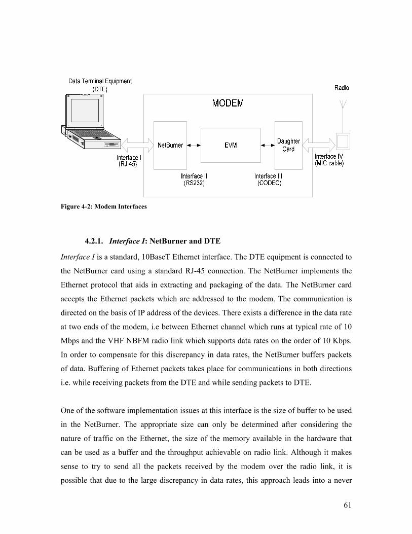
61
Figure 4-2: Modem Interfaces
4.2.1. Interface I: NetBurner and DTE
Interface I is a standard, 10BaseT Ethernet interface. The DTE equipment is connected to
the NetBurner card using a standard RJ-45 connection. The NetBurner implements the
Ethernet protocol that aids in extracting and packaging of the data. The NetBurner card
accepts the Ethernet packets which are addressed to the modem. The communication is
directed on the basis of IP address of the devices. There exists a difference in the data rate
at two ends of the modem, i.e between Ethernet channel which runs at typical rate of 10
Mbps and the VHF NBFM radio link which supports data rates on the order of 10 Kbps.
In order to compensate for this discrepancy in data rates, the NetBurner buffers packets
of data. Buffering of Ethernet packets takes place for communications in both directions
i.e. while receiving packets from the DTE and while sending packets to DTE.
One of the software implementation issues at this interface is the size of buffer to be used
in the NetBurner. The appropriate size can only be determined after considering the
nature of traffic on the Ethernet, the size of the memory available in the hardware that
can be used as a buffer and the throughput achievable on radio link. Although it makes
sense to try to send all the packets received by the modem over the radio link, it is
possible that due to the large discrepancy in data rates, this approach leads into a never
62
ending transmission loop. To elaborate on this issue, assume that the data throughput for
the radio link is 8 Kbps as shown in Figure 4-3. Next, consider that standard UDP/IP
packets are sent by the DTE to the modem and the buffer size is 100 packets. This means
that the NetBurner can buffer a maximum of 100 UDP/IP packets at any given instant.
The maximum size for UDP/IP packets, as defined in RFC standard [8] is 1472 bytes.
Assume that the size of each UDP packet in the buffer is 500 bytes which translates into
400 Kbits of data present in the NetBurner at any given instant. Now for the given
throughput of 8 Kbps over the radio link, it will take a minimum of 50 seconds for the
modem to empty the buffer. This represents the classical queuing theory problem in
which the input rate is more than output rate and hence requires a queue of infinite length
to ensure no loss of information. However an infinite queue will lead to a very large
latency. Thus, a trade off is required to be made between the permissible latency and the
queue size.
The nature of packet traffic is also important. Several packets may have a retransmit
frequency. Packet retransmission is generally associated with reliable internet protocols
like TCP/IP [26] which require all transmissions to be acknowledged. Now suppose that
the retransmit frequency for the current example is 10 seconds. Since it takes 50 seconds
for all of the messages to empty out of the buffer, this means that after 10 seconds the
sender would start retransmitting, adding duplicate messages to the buffer. In this case
transmitting both the packets is waste of bandwidth resources. This problem can be
avoided by ensuring that the application is aware of constraints of the air channel and
either a) doesn’t exceed the channel capacity or b) includes application-level handshaking
to avoid the problem.

63
Figure 4-3: Modem buffer size.
4.2.2. Interface II: NetBurner and EVM
The NetBurner card and the EVM are connected using an RS-232 link. The
communication between the NetBurner and the EVM consists of data signals and flow
control signals. The data signals refer to the information bits which are transmitted
between two modems. The flow control signals are used to regulate the flow of data
between the EVM and the NetBurner. There are two ways of implementing flow control
viz. hardware flow control and software flow control. The hardware flow control
mechanism consists of use of RS-232 interfacing pins. The software flow control
involves exchanging data patterns (special ASCII characters) to regulate data exchange.
The current system implements a simplified version of software flow control. The details
of the control signal implementation are given in Chapter 5. The flow control signals are
interchangeably referred to as handshaking signals or handshaking codes in this thesis.
The NetBurner transmits the Internet protocol packets over the serial port using Interface
II to the EVM. The EVM then modulates these raw data bits using the modules described
in Chapter 3. The EVM also demodulates the audio band OFDM symbol into raw data
bits and transmits it over Interface II to the NetBurner card for repackaging into standard
Ethernet protocol packets. The packaging and repackaging of Internet packets are
explored in more details Section 4.3 and Chapter 5. This notion of packaging and
repackaging of data implies that the data format transmitted between the radios need not
be identical to the data format received via the Ethernet port. Indeed, significant gains in

64
efficiency can be obtained if the received IP packets are reorganized, or packaged, prior
to transmission (which, of course, requires repackaging to negate the effects of the
reorganization upon reception). The details of these two actions are a part of the
transmission and receive modes/states of the modem. These details will be enunciated in
Chapter 6.
4.2.3. Interface III: EVM and Daughter Card
The radios used for FM transmission have certain requirements with respect to the input
and output signals so as to ensure optimal performance of the system. The daughter card
ensures that the signals at the output of the EVM are compatible with the radio. There are
three signals routed between the EVM and radios via the daughter card. The first signal is
the Push-To-Talk (PTT) signal. The radio is capable of communication in half duplex
mode only. The PTT signal is used for switching the radio between the transmit mode
and receive mode. The assertion of PTT signal switches the radio into transmit mode
while the deassertion shifts it back to the default receive mode. The implementation of
the PTT signal is discussed in detail in the Appendix A. The next interfacing signal is
between the audio output on the EVM and the microphone input of the radio via
daughter card. As described in Chapter 2, the strength of the modulating signal influences
the bandwidth of the FM signal. There exists an optimum level for input signal at the
microphone terminal of the radio to maximize the efficiency of the FM transmission and
avoid saturation. The audio output of the EVM is adjusted so as to meet this requirement
by use of appropriate circuitry as described in Appendix I. The final interfacing signal of
Interface III is between the speaker out of the radio and the audio input of the EVM. As
this is a high-level audio output, meant to drive a loudspeaker, and may need to be
modified to compensate for drive, impedance or DC offset..
4.2.4. Interface IV: Daughter Card and Radio
The same sets of signals at Interface III are repeated at Interface IV. The media between
the radio and the daughter card varies depending upon the radio used. It can be a simple
audio jack or a modified RJ-45 connector.
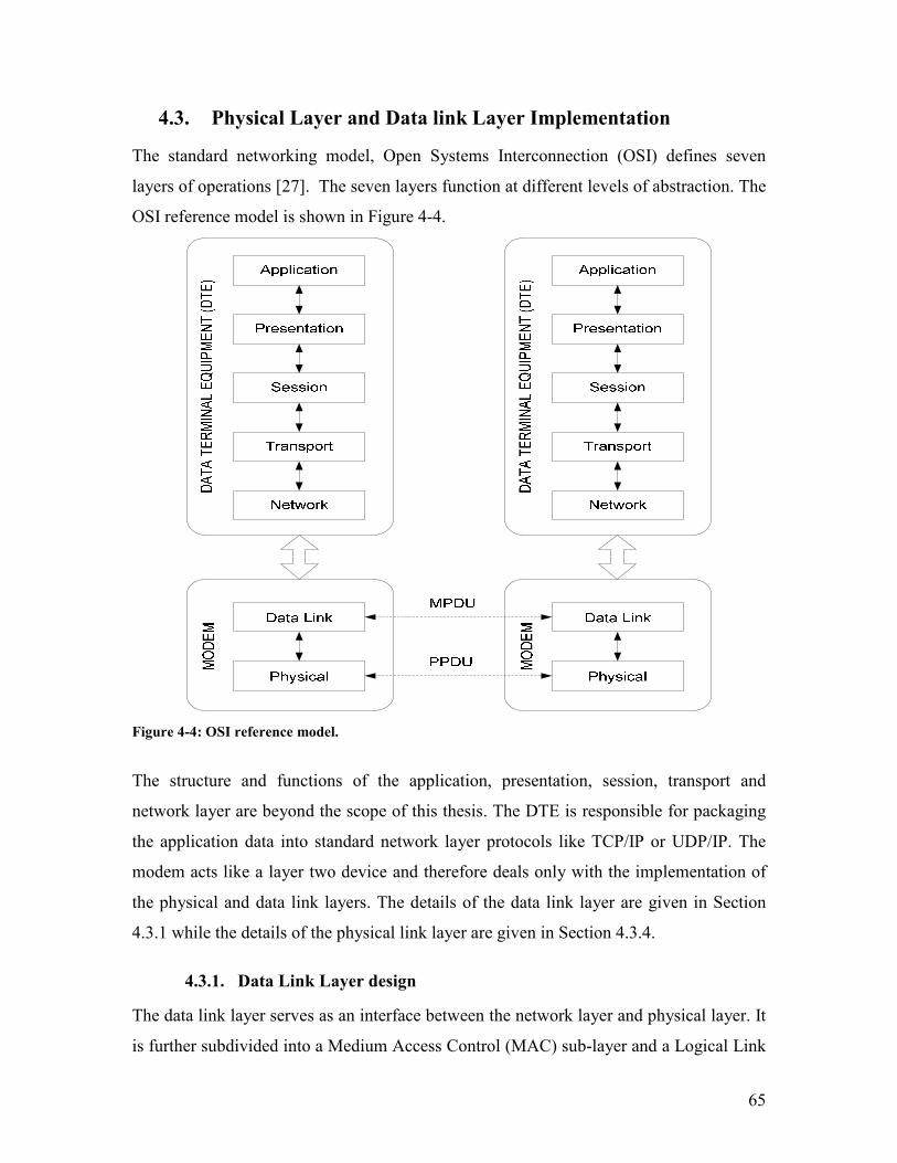
65
4.3. Physical Layer and Data link Layer Implementation
The standard networking model, Open Systems Interconnection (OSI) defines seven
layers of operations [27]. The seven layers function at different levels of abstraction. The
OSI reference model is shown in Figure 4-4.
Figure 4-4: OSI reference model.
The structure and functions of the application, presentation, session, transport and
network layer are beyond the scope of this thesis. The DTE is responsible for packaging
the application data into standard network layer protocols like TCP/IP or UDP/IP. The
modem acts like a layer two device and therefore deals only with the implementation of
the physical and data link layers. The details of the data link layer are given in Section
4.3.1 while the details of the physical link layer are given in Section 4.3.4.
4.3.1. Data Link Layer design
The data link layer serves as an interface between the network layer and physical layer. It
is further subdivided into a Medium Access Control (MAC) sub-layer and a Logical Link
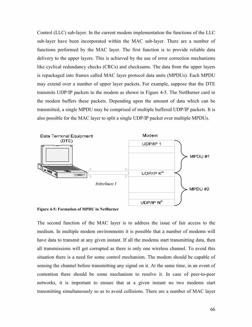
66
Control (LLC) sub-layer. In the current modem implementation the functions of the LLC
sub-layer have been incorporated within the MAC sub-layer. There are a number of
functions performed by the MAC layer. The first function is to provide reliable data
delivery to the upper layers. This is achieved by the use of error correction mechanisms
like cyclical redundancy checks (CRCs) and checksums. The data from the upper layers
is repackaged into frames called MAC layer protocol data units (MPDUs). Each MPDU
may extend over a number of upper layer packets. For example, suppose that the DTE
transmits UDP/IP packets to the modem as shown in Figure 4-5. The NetBurner card in
the modem buffers these packets. Depending upon the amount of data which can be
transmitted, a single MPDU may be comprised of multiple buffered UDP/IP packets. It is
also possible for the MAC layer to split a single UDP/IP packet over multiple MPDUs.
Figure 4-5: Formation of MPDU in NetBurner
The second function of the MAC layer is to address the issue of fair access to the
medium. In multiple modem environments it is possible that a number of modems will
have data to transmit at any given instant. If all the modems start transmitting data, then
all transmissions will get corrupted as there is only one wireless channel. To avoid this
situation there is a need for some control mechanism. The modem should be capable of
sensing the channel before transmitting any signal on it. At the same time, in an event of
contention there should be some mechanism to resolve it. In case of peer-to-peer
networks, it is important to ensure that at a given instant no two modems start
transmitting simultaneously so as to avoid collisions. There are a number of MAC layer
67
protocols which make provisions to prevent and at the same time detect such collisions.
The most frequently used implementations are Carrier Sense Multiple Access with
Collision Detection (CSMA/CD) which is described in Section 4.3.2 and Carrier Sense
Multiple Access with Collision Avoidance (CSMA/CA) which is described in Section
4.3.3 [14].
4.3.2. CSMA/CD
This medium access control technique is widely used in the IEEE 802.3x Ethernet
standard. A single Ethernet network may be used to provide access to a group of attached
terminals. All these terminals are said to form a collision domain. To control which
terminals should be allowed to transmit at a given instant, a protocol is needed. In the
absence of this protocol all the terminals which have data to be sent will start
transmitting, resulting in loss of data. As the name suggests, in carrier sense multiple
access protocols all the terminals have to listen to the channel before they start
transmitting. If they sense a transmission on the desired channel they will not transmit
their data. Instead they will wait for the channel to be inactive. However this technique
alone cannot guarantee an error free transmission. This is because if two terminals start
transmitting near simultaneously, then they could both see an idle channel and
simultaneously conclude that no other terminal is transmitting. This will result in
collision and eventually the corrupted transmission will have to be discarded.
In order to detect that a collision has occurred a second technique known as collision
detection is used in conjunction with CSMA. In this method every terminal monitors the
physical medium during its own transmission. If it senses a collision it immediately stops
transmitting and sends a jamming sequence. The purpose of the jamming sequence is to
ensure that the remaining terminals will discard the frame. In the case of Ethernet, the
collision detection is implemented by observing the current levels on the cable medium.
All the parameters for the cable medium are predefined such that the limits on signal
strength are known. This knowledge can be used for detecting collisions. However if the
medium is wireless then it becomes impossible to detect collisions. In such situation a
different scheme is implemented.

68
4.3.3. CSMA/CA
This medium access control is implemented in IEEE 802.11x wireless LAN standard [14]
[28]. A CSMA/CA protocol has been designed to reduce the collision probability
between multiple terminals accessing the same medium, at the point where collision will
most likely occur. Just after the medium becomes idle, following a busy medium (as
detected by the carrier sensing), is when the highest probability of collisions exists. This
is because multiple terminals might have been waiting to transmit. This means that once
the channel goes idle many transmitters may wish to send the data they’ve been holding
while waiting for the channel to clear. This situation necessitates the use of a random
backoff procedure to resolve the medium contention issues. The random backoff requires
that once the channel clears, each transmitter wait an additional, randomly selected,
backoff time. This improves the possibility that that no contention takes place between
the terminals.
4.3.4. Physical Layer (PHY) design
The physical layer acts as an interface between the data link layer and the channel. The
channel in this context refers to the radio link used by the radios. The PHY layer has to
provide three levels of functionality. First, the PHY layer provides a data exchange
mechanism between the upper layers and PHY layer. The MAC layer transmits MPDUs
to the PHY layer.
Depending upon a number of physical constraints, like requirements for synchronization
and equalization, which were described in Chapter 2, it may not be advisable to transmit
the entire MPDU. For example, in block type pilot equalization described in Chapter 2,
the channel frequency response is calculated over the training symbol. The remaining
symbols are equalized using this channel response measurement. There is an inherent
assumption that the channel remains invariant over the duration of transmission. In such
scenarios it is useful to periodically insert training symbols to take in account the
variations in the channel.

69
For the reasons discussed above, each MPDU is broken down into a number of PHY
layer protocol data units (PPDUs). There are two ways of forming a PPDU; one will be
fixed length while other one will be variable length. The main reason for using variable
length PPDUs is to avoid the wasting transmission bandwidth which is at a premium.
However this requires some mechanism of communicating the size of the PPDU, which
adds data overhead. The second approach of having a fixed length for PPDU is easier to
implement. As shown in the Figure 4-6, each PPDU consists of a header which is the
training sequence used in equalization and data field.
Figure 4-6: Formation of a PPDU from MPDUs.
The second functionality of the PHY layer deals with the modulation and demodulation
of the data. This includes the modules described in Chapter 3. The data payload shown in
Figure 4-6 will be audio band OFDM symbols generated by the modulator.
The third function of the PHY layer is to provide a carrier sense mechanism to the upper
MAC layer. The carrier sensing mechanism was discussed in detail in Sections 4.3.2 and
4.3.3 .
70
5. SYSTEM IMPLEMENTATION
Chapters 3 and 4 described the construction and system design of a modem which creates
an interface between data terminal equipment (DTE) and a land-mobile radio (LMR). In
this chapter, the design and implementation is further narrowed down with respect to the
specific DREAMS application. The DREAMS application and software was introduced
in Chapter 1. The nature of this software influences various parameters like the size of
buffer on the NetBurner and back off time in the CSMA/CA algorithm, all of which were
articulated in Chapter 4. In addition to dealing with specific software applications on the
DTE, the implemented system assumes the use of an NBFM analog radio working in half
duplex mode for the rest of the discussions. Similar principles are applicable to other
analog radio channels.
5.1. System Overview: DREAMS and the OFDM Modem
The DREAMS software was primarily designed to facilitate interaction between a
paramedic working in a mobile ambulance and a physician stationed at a hospital or a
base camp. The paramedic station is capable of monitoring a number of important
physiological signs which can be of assistance to the physician for correct diagnosis. In
order to transfer this information, a radio link can be chosen amongst the available
communication technologies like cell phones, satellites and, with the modem, land mobile
radio. A detailed description was given in Chapter 1.
Figure 5-1 shows a typical configuration of such a system. As seen in the figure,
Terminal 1 is interfaced with Modem 1 via an RJ-45 connection. Modem 1 is, in turn,
connected to the land mobile radio. Similarly Terminal 2 is interfaced with Modem 2
which is also connected to a radio. The communications between the terminal and the
modem and vice-versa is carried out using UDP/IP packets.

71
Figure 5-1: DREAMS system setup
The choice of the UDP/IP protocol was a project requirement which was established to
ensure interoperability with the DREAMS software. The DREAMS software used the
UDP/IP protocol for all data transfers. Furthermore, in the current implementation,
communications is restricted between the modem and the terminal interfaced with it. That
is to say that all the packets which are to be transmitted by the terminal are sent to the IP
address of the modem and similarly all the packets which are received by the modem are
sent to the IP address of the connected terminal. This was also a project requirement since
the DREAMS application did not to keep a track of the IP addresses of other terminals in
the system.
Each modem has a static IP address as the terminals used in DREAMS system do not
support the DHCP protocol [29]. The IP addresses of the interfaced terminals are also
hard coded in the modems for the current configuration. The modem software is
independent of the type of terminal being interfaced, that is to say that any modem can be
interfaced with the Paramedic or Physician station. The modem identifies each station
only on the basis of the IP address; the nature of data transmitted from either terminal
does not require any change in the design of the software.
All that is required to remove the above restrictions is to implement a more complete
protocol stack in the NetBurner.

72
The DREAMS software, as mentioned previously, is capable of transmitting a range of
physiological and communications (audio, video and text) data. Each type of data source
can be considered as a separate application. All the applications are uniquely identified
by the UDP port numbers they use and by the statistics of the data they generate in terms
of size and frequency. Identification of the data source is required by the DREAMS so as
to prioritize the data generated. For example, transmitting ECG information will be of a
greater importance than the transmission of any telemetry information. The prioritization
of data is accomplished in the DREAMS software itself, and is beyond the scope of this
thesis as it is completely transparent to the modems. The modems communicate with
each other using the land mobile radio link which in the current implementation, was a
pair of Motorola XTS 5000 VHF radios operating in their analog mode.
5.2. System Interface:
This section gives the detailed design and implementation for the different interfaces in
the modem. These interfaces were introduced in Chapter 4. Each of these interfaces have
been tailored in accordance with the requirements and constraints of the DREAMS
application and the land mobile radio.
5.2.1. Interface I: NetBurner and DREAMS
This is the standard Ethernet interface. An overview of this interface was given in
Chapter 4. The DREAMS terminal and the modem exchange information in the form of
UDP/IP packets. Figure 5-2 shows the contents of a standard UDP header [8].

73
Figure 5-2: User Datagram (UDP) header format.
As seen in the figure, the UDP header contains source port and destination port address
fields. These addresses are different from the IP addresses which are used to direct
packets between the modem and the DREAMS terminals. The length field in the UDP
header indicates the size of the data payload while the checksum is used to ensure that no
errors have occurred during the transmission.
It was mentioned in Section 5.1 that there are number of physiological and telemetry
signals which are exchanged between the physician and paramedic terminals, and there is
need to uniquely identify the data types. The source and destination ports numbers serve
this purpose. For example any traffic on source port number 4200 indicates data from the
navigation server and any traffic on source port number 4100 indicates ECG server data.
Table 1-2 provides a more comprehensive list of the services and the associated port
numbers.
The modem, although oblivious to the nature of the data, is required to accept UDP
packets only in a certain range of port addresses. The reason for this is that the DREAMS
system requires addresses in certain range (port numbers above 6000) for communicating
with different modules which are not a part of the modem. For reasons of backward
compatibility, no changes were made in DREAMS software. Instead, the modem receives
and transmits traffic on port numbers between 3000 and 6000 and ignores traffic on all
other ports, even if the traffic is sent to the modem’s IP address.

74
It is important to mention that the modem appears completely transparent to the
DREAMS system. This is to say that the integrity of the UDP packets is guaranteed,
meaning that a UDP packet is either delivered correctly, or it is dropped completely. Any
acknowledgements required are done by the DREAMS software.
The next important interface parameter is the buffer size. The NetBurner uses a buffer
size of 200 UDP/IP packets. Each packet can vary in length up to the maximum
permissible size of 1472 bytes as defined in the standard. Choosing the number of
packets to be buffered is a tradeoff between the throughput achievable over the radio link
and the duration of the transmission or receive time slots for the modem. The LMR works
in half duplex mode, which means that the modem can be either in the transmit mode or
receive mode at any given instant. A single transmission or receive slot lasts for duration
of not more than 6 seconds (a value deemed to be a reasonable tradeoff between average
data rate and channel utilization). The details on the make up and duration of the slots
will be given Chapter 6. The on-air throughput for the current modem stands at about
3000 bits per second. Figure 5-3 shows the details for Interface I. The throughput
calculation is based on the factors like the makeup of the transmission slot, data rate
achievable over the radio link all of which are described in Chapters 6, 7 and 8.
Figure 5-3: A desktop which runs DREAMS application is connected to the modem using RJ 45
connection (Interface I.).
75
From the above analysis it can be derived that the maximum number of bytes that can be
transmitted in a single slot which has a maximum duration of 6 seconds and throughput
of 3 kbps, is about 1800 bytes. Thus the buffer is selected such that at any given instant it
should be able to house a minimum of 1800 bytes. Given the overhead associated with
each UDP message if each UDP/IP had just 1 byte as the payload, then it would take
about 80 UDP/IP packets to fill up a single slot. Thus, the selected number 200 satisfies
this constraint. For a more detailed analysis on implementation of buffers, please refer to
reference [30].
5.2.2. Interface II: NetBurner and EVM
This is a standard RS-232 interface. The signals exchanged between the NetBurner and
the EVM can be classified into two types viz. data signals and control signals as
discussed previously in Chapter 4. The control signals are required to ensure proper
exchange of data between the EVM and NetBurner. This section elaborates the
implementation of such a control signaling scheme.
As mentioned in Section 5.1, the modems have three distinct operating modes as shown
in the state diagram of Figure 5-4, the “listen” mode (State 0), the “receive” mode (State
1) and the “transmission” mode (State 2). Due to the half duplex nature of radio link, the
modem never receives and transmits at same instant. The listen state is a default state for
the modem. This is to say that the modem is always listening for a transmission on the
radio link/channel. If a signal is received, it is demodulated using the modules described
in Chapter 3. The demodulated data bits are then sent to the NetBurner. This process is
augmented with the exchange of suitable handshaking signals/codes. The modem will
enter into transmission mode only upon the assertion of the two conditions, first there
must be no activity on the channel and second there must be data available for
transmission. The channel idleness is confirmed by the implementation of the MAC layer
protocol to be discussed in Section 5.3.1. In order to confirm availability of data,
handshaking/flow control signals are needed.
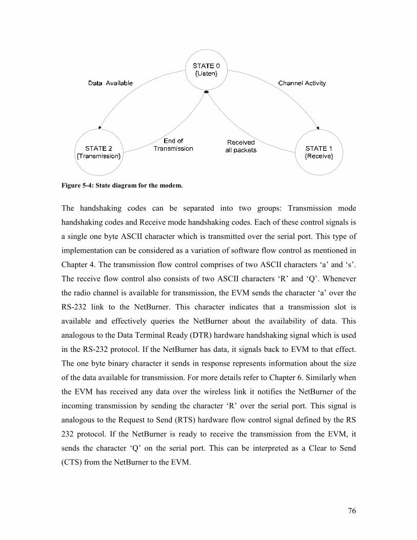
76
Figure 5-4: State diagram for the modem.
The handshaking codes can be separated into two groups: Transmission mode
handshaking codes and Receive mode handshaking codes. Each of these control signals is
a single one byte ASCII character which is transmitted over the serial port. This type of
implementation can be considered as a variation of software flow control as mentioned in
Chapter 4. The transmission flow control comprises of two ASCII characters ‘a’ and ‘s’.
The receive flow control also consists of two ASCII characters ‘R’ and ‘Q’. Whenever
the radio channel is available for transmission, the EVM sends the character ‘a’ over the
RS-232 link to the NetBurner. This character indicates that a transmission slot is
available and effectively queries the NetBurner about the availability of data. This
analogous to the Data Terminal Ready (DTR) hardware handshaking signal which is used
in the RS-232 protocol. If the NetBurner has data, it signals back to EVM to that effect.
The one byte binary character it sends in response represents information about the size
of the data available for transmission. For more details refer to Chapter 6. Similarly when
the EVM has received any data over the wireless link it notifies the NetBurner of the
incoming transmission by sending the character ‘R’ over the serial port. This signal is
analogous to the Request to Send (RTS) hardware flow control signal defined by the RS
232 protocol. If the NetBurner is ready to receive the transmission from the EVM, it
sends the character ‘Q’ on the serial port. This can be interpreted as a Clear to Send
(CTS) from the NetBurner to the EVM.
77
5.3. Physical (PHY) Layer and Medium Access Control (MAC)
Layer Implementation
The functions of the physical layer and medium access layer were discussed in Chapter 4.
In this section the implementation of the physical and MAC layer is described with
context of the DREAMS application. The performance of the modem can be improved if
certain characteristics of the DREAMS software are exploited. The modifications made
will be discussed in Sections 5.3.1 and 5.3.2.
5.3.1. MAC Layer Implementation
As described in Chapter 4, there are two important functions for the MAC layer. The first
is to ensure reliable data transfer; the second is to guarantee fair access to the channel
resources. The interfaced terminals communicate using UDP/IP packets which are
buffered by the NetBurner as described in Section 5.2.1. The buffered packets are used to
form an MPDU packet. The packets are processed according to last in first out (LIFO)
basis. The NetBurner further maintains a record of the number and size of UDP/IP
packets it receives. The design and implementation of the buffer is beyond the scope of
this thesis and more details on the process are available in reference [30]. There exists a
maximum limit on the size of the MPDU. This limit is governed by the maximum
permissible transmission slot time and data throughput achievable. Accordingly it is
possible for the MPDU to contain more than one UDP/IP packet. Further it is possible
that a single UDP/IP is split over two consecutive MPDUs. Reliability is achieved by
appending parity bits at regular intervals. For more details on the fragmentation and
defragmentation of UDP/IP packets to form an MPDU and to provide error detection
capabilities refer to reference [30].
In order to preserve the bidirectional nature of the half-duplex link, it is important to
ensure that every terminal gets an opportunity to transmit data. The modem currently
implements a version of CSMA/CA, described in Chapter 4, to ensure fair access and
avoid collisions. From Section 5.2.2, it was observed that in the default state the modem
always monitors the channel for any activity. At the same time the EVM is periodically
querying the NetBurner for any data that needs to be transmitted. The NetBurner

78
indicates the presence of data through exchange of appropriate handshaking codes. Each
modem listens to the channel before beginning any transmission. Once the data
availability is ascertained, the EVM implements a random backoff algorithm. This is to
say that it will continue to monitor the channel for a random amount of time before
occupying the channel. This random backoff is similar to the one used in CSMA/CD.
However in CSMA/CD the random backoff is implemented after any collision has been
detected. In case of a wireless, half duplex, medium it is not possible to detect collisions
and hence the random backoff implemented serves as a collision avoidance technique.
At the end of the random backoff, the modem starts transmitting. If the modem senses
any activity on the channel during the backoff period it will abandon the transmission of
the scheduled data. This implementation will be explained in the context of the
transmission and receive slots which will be described in Chapter 6. Collision avoidance
is achieved as the probability of collision for the system is highest at the end of the
previous transmission. In addition the random backoff is biased so that the station which
was transmitting most recently is given a lower priority for transmission in the next
available slot. This design for the MAC layer has been influenced by the working of the
interfaced DREAMS software. In the DREAMS software, the data traffic occurs in bursts
using the UDP protocol. The UDP protocol falls in the family of unreliable networking
protocols. For details on unreliable protocols refer to reference [8]. However, certain data
transfers might demand reliability. An example of such a service is the patient database.
Every field of the database is required to be reliably transmitted. Thus any UDP/IP packet
which encapsulates database data has to be acknowledged by transmission of another
UDP/IP packet by the receiving DREAMS terminal as a mechanism of enforcing
reliability. In absence of the bias on the backoff, it is possible that the received station
does not get a chance to transmit an acknowledgement which results in retransmission of
the same packet over the channel.
Figure 5-5 shows such a scenario. Part (a) displays the events when no bias exists while
part (b) displays the events with bias on random backoff. For this discussion, assume that
the applications on Paramedic station (Modem 1) generated UDP/IP packets which are to

79
be transmitted to the Physician terminal. To achieve this, the packets will first be
transmitted to Modem 1 which has a unique IP address. The NetBurner in Modem 1
receives these packets and buffers them in the UDP buffer. Without loss of generality,
assume that the total number of bytes in the all packets is less than the maximum that can
be transmitted in a single transmission slot. It is important to note that both the modems
run asynchronously with each other and that the default state for both these devices is the
listening state as seen in Figure 5-4. The EVMs on both the modems are also periodically
querying the respective NetBurners for data. In consistence with the assumption about
paramedic station made earlier, the NetBurner in Modem 1 signals to the EVM about the
availability of data for transmission. Next, the EVM in Modem 1 will transmit the MPDU
which has been translated into equivalent PPDUs represented by P1, over the wireless
link. The EVM in Modem 2, which is functioning in its default listen mode, starts
receiving the signal. After handshaking with the EVM, the NetBurner in Modem 2 starts
reassembling the UDP packets. It then transmits the UDP/IP packets to the Physician
terminal. The applications on the Physician station generate acknowledgements, ACK 1,
for the received UDP packets.
Figure 5-5: Half duplex communication (a) without bias on random back off (b) with bias on
random backoff .
Now consider the possibility that Modem 2 gets an opportunity to transmit the
acknowledgement. Once this acknowledgement is received before the expiration of

80
retransmit window, the paramedic station starts sending the next set of UDP/IP packets
which are a part of PPDU represented by P2. Upon receiving the data, the physician
station generates another acknowledgement packet ACK 2. However, due to the
randomness involved, the paramedic station retransmits P2 at the end of backoff period.
Thus packet P2 transmission is duplicated which wastes bandwidth resources. Another
option to resolve this issue would be to modify the retransmit frequency at the paramedic
terminal. However even this option does not guarantee the transmission of
acknowledgement, it merely delays the retransmission of the duplicate packet.
The bias on the random backoff equates roughly to the Physician station getting a higher
priority for next transmission slot. So although both modems may enter into the random
backoff algorithm at the same time, one of them will start transmitting a sufficient time
ahead of the other one. To generalize the implementation, the modem which transmitted
the most recently will be given a lower priority for transmission on the next slot as
compared to the modem which was in receive mode. The main motivation for this
modification is the nature of interaction between the DREAMS software on paramedic
and physician terminals discussed in Chapter 1. Other applications may require a
different tradeoff.
5.3.2. Physical Layer Implementation
The functionalities of the physical layer were elucidated in Chapter 4. The transfer of
modulated data bits is accomplished using PPDUs. The PPDUs are derived from MPDUs
and a single MPDU can be split over single or a multiple PPDUs depending upon its size.
The size of each PPDU is fixed to seven symbols. The first symbol is comprised of
header data while the subsequent symbols are generated from data bits using the modules
described in Chapter 3. The header functions as a training symbol used for equalizing the
channel. Figure 5-6 shows the contents of a single PPDU.

81
Figure 5-6: Physical layer protocol data unit (PPDU).
Every OFDM data symbol is generated from 24 unprocessed data bytes. For details on
the data conditioning and modulation schemes and the process of conversion of 24 data
bytes into single baseband OFDM symbol please refer to Chapter 3. This means that
every PPDU contains 144 data bytes. These data bits are actually the bits that make up
the MPDU. Thus a single MPDU is sliced up into blocks of 144 bytes to form a string of
PPDUs. In an event that there are less than 144 bytes available to form a PPDU, zero
padding is used. Figure 5-7 shows the process of forming PPDUs.
Figure 5-7: Physical Layer Protocol Data unit formation.

82
Consider that there is a MPDU packet which is made up of 648 bytes. As discussed in
Section 5.2.1, the MPDU may consist of one or more UDP/IP packets. During PPDU
formation, 144 bytes of the MPDU are converted into six data symbols. As seen in Figure
5-7, for the fifth PPDU only 72 bytes of MPDU are available. Because of the need for a
fixed length implementation of a PPDU, 576 zero bits (72 zero bytes) are appended to the
MPDU. This makes the length of the last PPDU equal to the required number of symbols.
The maximum number of PPDUs and hence the maximum permissible size of MPDU is
dictated by the data rate of the channel. As such, a tradeoff must be made between the
maximum number of PPDUs permitted in a single transmission slot and the efficiency of
the system. A detailed discussion is presented in Chapter 6.

83
6. SOFTWARE ARCHITECTURE
Chapter 5 introduced the design and implementation of the modems interfaced with the
DREAMS software. This chapter articulates the design of features like the transmit and
receive slots and PPDUs. As described before, due to the half duplex nature of a land
mobile radio, the modem can be in the transmit mode or the receive mode, but may never
simultaneously transmit and receive. In Section 6.2, the transmit slot has been described
in detail. Section 6.4 discusses the tradeoffs involved in increasing the duration of
transmit slot and minimizing channel occupancy. The makeup of the receive slot has been
explained in Section 6.3. As mentioned in Chapter 5, the transmitting and receiving
modem are synchronized with each other for the duration of transmit/receive slot. Section
6.5 gives a broad overview of the handshaking codes exchanged during transfer of
PPDUs between the modems over the radio channel.
6.1. Working of the system
As described in Chapter 5, the modems will be in the “listen” state by default. Consider a
general setup as shown in Figure 6-1. Although the discussion includes a single
transmitter and receiver pair, the same concepts can be extended to multi-terminal
scenarios. The changes involved will be discussed in Chapter 9.
Figure 6-1: Working of System.

84
Assume that the application on the paramedic terminal sends UDP/IP packets to
Modem 1. The NetBurner in Modem 1 buffers these packets. The NetBurner now has
data and will respond upon receiving the handshaking codes, which is an appropriate
ASCII character as discussed in Chapter 5, from the EVM of Modem 1. Next, the
NetBurner calculates the size of a single MPDU in units of PPDUs it contains and
communicates that number to the EVM as a part of the handshaking protocol. The
purpose of this transfer is explained later in Section 6.4 . Referring to the example of
Figure 5-7, a single PPDU consists of six data symbols and one header symbol. The six
24 byte data symbols were formed from 144 bytes which were part of a larger MPDU.
There exists a limit, based on the desired maximum amount of time the channel is
occupied, to the maximum number of PPDUs which can be transmitted in a single slot.
For the current implementation, this limit is 12 PPDUs. A more detailed discussion on
this number is available in Section 6.4. Thus, the maximum size of an MPDU is limited
to 1724 bytes. A single MPDU can encompass multiple UDP packets. Furthermore, it can
also contain a single partial UDP packet. Details on the procedure for the formation of an
MPDU are given in reference [30]. The EVM modulates the data bits received from the
NetBurner via Interface II as described in Chapter 4 to form PPDUs. The PPDUs are then
transmitted by the radio. Before starting the transmission, the EVM has to signal the
radio, half duplex by design, to shift to transmit mode. This is switching is accomplished
by assertion and deassertion of the Push-To-Talk (PTT) line available on the radio. The
EVM is interfaced with this feature via Interface III and Interface IV, as discussed in
Chapter 4. These operations constitute the Transmit slot.
Upon the reception of a signal, the EVM on Modem 2, starts demodulating the received
PPDUs into data bits using the demodulation modules described in Chapter 3. At the
same time, the NetBurner in the receiving modem, is notified of the incoming
transmission by use of the handshaking codes described in Chapter 4. The NetBurner
starts receiving the data bits over the transmit slot to obtain an entire MPDU. Next it
retrieves one or more UDP packets which may be complete or partial. If a partial UDP
packet is received, the NetBurner stores the partial UDP in a temporary buffer. For details
on this process, please refer to reference [30]. The NetBurner encapsulates each UDP

85
packet into an Ethernet frame and relays the data to the connected Physician terminal
over the RJ-45 connection. These operations constitute the Receive slot.
The summary of protocol packets exchanged is shown in Figure 6-2. A direct one-to-one
correspondence can be drawn between most of the constituents of Transmit and Receive
slots. The only difference is the operations being performed in the respective time
intervals.
Figure 6-2: Protocol Packets exchanged between different layers.
Also the modem transmitting the PPDU packets and the modem receiving the packets are
synchronized for the duration of the transaction. This means that the transmit slot and the
receive slot start at near simultaneous instants and exist for almost the same duration.
6.2. Transmit Slot
From the discussions in Section 6.1, it is seen that the EVM of the transmitting modem
asserts the PTT signal at the beginning of the transmit slot. The term, transmit slot
encompasses the time duration from the instant of assertion of PTT to the deassertion of

86
PTT. It can be further subdivided into a TX_KEY interval, a PPDU interval, an inter-
PPDU Interval, an End of Transmission Interval and a TX_UNKEY interval. Figure 6-3
shows these subdivisions in the context of a transmitted waveform. The duration of each
of these sub intervals is given in Table 9-1.
Figure 6-3: Transmit Slot as seen at the input of Modem which is connected to a Motorola XTS 5000
radio.
6.2.1. TX_KEY Interval
Whenever any signal is transmitted, the Push to Talk (PTT) switch on the transmitting
radio must be asserted (also known as “keying” the radio). On assertion of this switch,
the microphone input on the radio serves as an input for transmitting data. On the
receiving end, the radio is unsquelched upon detection of a valid carrier. This transition
from being squelched to being unsquelched generates a transient pulse at the receiving
radio. Figure 6-4 shows an example of a transient observed on a Motorola XTS5000
radio when used in conjunction with the modems. The duration of the pulse is a function
of the interfacing logic and characteristics of the radio used. It is necessary to wait until
this transient pulse has died down before the PPDUs are actually transmitted. In the event
that the PPDU transmission overlaps with the pulse, the demodulated data will be
corrupted and this will result in errors in the received PPDU and eventually errors in the
MPDU packet.

87
Figure 6-4: Transient pulse observed at the modem during PPT assert.
6.2.2. PPDU Interval
Once the initial transient has died down at the end of TX_KEY interval, we start
transmitting an audio bandwidth OFDM signal from the EVM. In a single transmit slot it
is possible to transmit multiple PPDUs. The time interval corresponding to a single
PPDU is referred to as the PPDU Interval. The duration of this interval will depend upon
the data rate achievable over the channel and size of the PPDU. The number of PPDU
intervals in a single transmit slot varies depending upon the size of the data to be
transmitted over the channel.
6.2.3. Inter-PPDU Interval
In addition to the PPDU intervals, the transmit slot may contain inter-PPDU intervals.
No data signal is transmitted in this interval. During this interval the receiver algorithm
and the transmitter algorithms, which will be explored in detail in Chapter 7, reinitialize.
6.2.4. End of Transmit Interval
This interval is similar to the Inter-PPDU Interval and follows the final PPDU
transmission. No data is transmitted in this interval either. However the purpose of this
interval apart from software initialization is to indicate the last PPDU transmission.
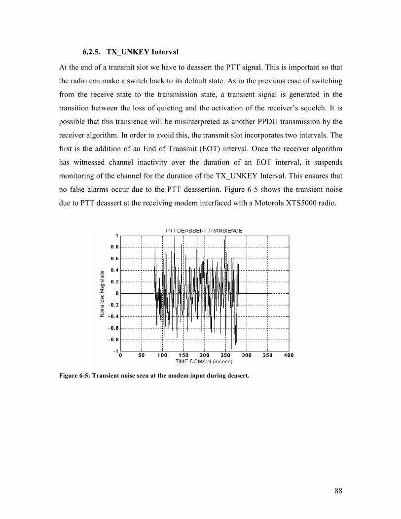
88
6.2.5. TX_UNKEY Interval
At the end of a transmit slot we have to deassert the PTT signal. This is important so that
the radio can make a switch back to its default state. As in the previous case of switching
from the receive state to the transmission state, a transient signal is generated in the
transition between the loss of quieting and the activation of the receiver’s squelch. It is
possible that this transience will be misinterpreted as another PPDU transmission by the
receiver algorithm. In order to avoid this, the transmit slot incorporates two intervals. The
first is the addition of an End of Transmit (EOT) interval. Once the receiver algorithm
has witnessed channel inactivity over the duration of an EOT interval, it suspends
monitoring of the channel for the duration of the TX_UNKEY Interval. This ensures that
no false alarms occur due to the PTT deassertion. Figure 6-5 shows the transient noise
due to PTT deassert at the receiving modem interfaced with a Motorola XTS5000 radio.
Figure 6-5: Transient noise seen at the modem input during deasert.
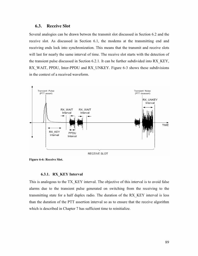
89
6.3. Receive Slot
Several analogies can be drawn betwen the transmit slot discussed in Section 6.2 and the
receive slot. As discussed in Section 6.1, the modems at the transmitting end and
receiving ends lock into synchronization. This means that the transmit and receive slots
will last for nearly the same interval of time. The receive slot starts with the detection of
the transient pulse discussed in Section 6.2.1. It can be further subdivided into RX_KEY,
RX_WAIT, PPDU, Inter-PPDU and RX_UNKEY. Figure 6-3 shows these subdivisions
in the context of a received waveform.
Figure 6-6: Receive Slot.
6.3.1. RX_KEY Interval
This is analogous to the TX_KEY interval. The objective of this interval is to avoid false
alarms due to the transient pulse generated on switching from the receiving to the
transmitting state for a half duplex radio. The duration of the RX_KEY interval is less
than the duration of the PTT assertion interval so as to ensure that the receive algorithm
which is described in Chapter 7 has sufficient time to reinitialize.
90
6.3.2. RX_WAIT Interval
The RX_WAIT interval is the time during which the receiving modem is awaiting a valid
transmission. If the receiving modem starts receiving signal before the end of this
interval, it is interpreted as a valid transmission. Once the channel has been detected
silent for the entire duration of RX_WAIT interval, it is considered the end of
transmission. Thus, in the case of multiple PPDU transmission, a part of the RX_WAIT
interval overlaps the inter-PPDU interval as opposed to the End of Transmit (EOT)
interval at the end of transmission. A detailed algorithm on the detection mechanism
follows in Chapter 7.
6.3.3. PPDU Interval
This is same as the PPDU Interval of the transmit slot. In this interval the receiving
modem demodulates the PPDU symbols into the data bits that constitute an MPDU.
6.3.4. RX_UNKEY Interval
This interval overlaps with the TX_UNKEY interval. Thus, the main function of this
interval is to avoid a false alarm that may be generated by the transient noise caused by
the receiver’s squelch. During this interval, the receiver algorithm stops monitoring the
channel for activity. Any signal on the channel will go undetected during this interval.
Another alternative to this interval would be to demodulate the received transience noise
and transfer the data bits to the NetBurner as a part of an MPDU. Since the MAC layer
implementation as discussed in Chapter 5, has error detecting capabilities, the corrupted
data will be discarded. These issues will be discussed in Chapter 9.
6.4. Duration of Transmit and Receive Slot
The implementation of the physical layer was discussed in Chapter 5. The transfer of
data bits which are part of an MPDU is carried over Interface I using the handshaking
protocol described in Chapter 5. For the DREAMS system implementation, each PPDU is
comprised of one header symbol and six data symbols which translates into 144 bytes of
data. In a single transmit slot a single, or multiple, PPDUs can be transmitted. A tradeoff
must be made between the amount of data that can be transmitted and the amount of time
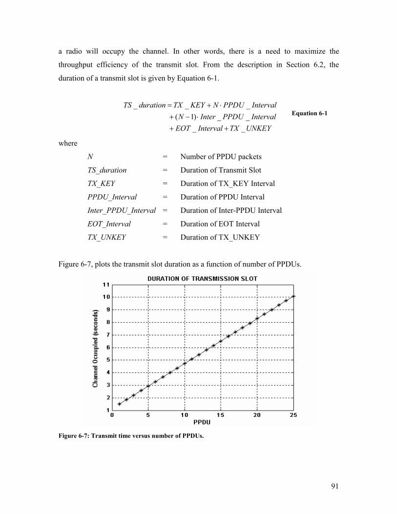
91
a radio will occupy the channel. In other words, there is a need to maximize the
throughput efficiency of the transmit slot. From the description in Section 6.2, the
duration of a transmit slot is given by Equation 6-1.
UNKEYTXIntervalEOT
IntervalPPDUInterN
IntervalPPDUNKEYTXdurationTS
__
__)1(
___
++
⋅−+
⋅+=
Equation 6-1
where
N = Number of PPDU packets
TS_duration = Duration of Transmit Slot
TX_KEY = Duration of TX_KEY Interval
PPDU_Interval = Duration of PPDU Interval
Inter_PPDU_Interval = Duration of Inter-PPDU Interval
EOT_Interval = Duration of EOT Interval
TX_UNKEY = Duration of TX_UNKEY
Figure 6-7, plots the transmit slot duration as a function of number of PPDUs.
Figure 6-7: Transmit time versus number of PPDUs.
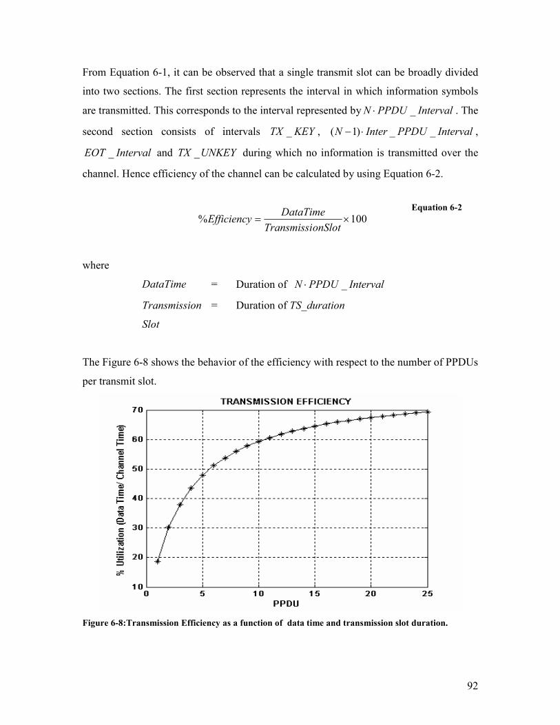
92
From Equation 6-1, it can be observed that a single transmit slot can be broadly divided
into two sections. The first section represents the interval in which information symbols
are transmitted. This corresponds to the interval represented by IntervalPPDUN _⋅ . The
second section consists of intervals KEYTX _ , IntervalPPDUInterN __)1( ⋅− ,
IntervalEOT _ and UNKEYTX _ during which no information is transmitted over the
channel. Hence efficiency of the channel can be calculated by using Equation 6-2.
100% ×=onSlotTransmissi
DataTimeEfficiency
Equation 6-2
where
DataTime = Duration of IntervalPPDUN _⋅
Transmission
Slot
= Duration of TS_duration
The Figure 6-8 shows the behavior of the efficiency with respect to the number of PPDUs
per transmit slot.
Figure 6-8:Transmission Efficiency as a function of data time and transmission slot duration.
93
From Figure 6-8 it can be observed that as the number of PPDUs in a single slot
increases, the efficiency improves. However, any increase in the number of PPDUs also
results in an increase in the duration of channel occupation as observed from Figure 6-7.
Thus, a tradeoff has to be made between the possible transmission efficiency and the
amount of time the channel is occupied. For the current design, the number of PPDUs
which can be transmitted in a single transmit slot is limited to twelve. This gives a
maximum achievable transmission efficiency of about 62% and a maximum channel
occupation time of 5.436 seconds. Therefore, although the number of PPDUs to be
transmitted is variable, it is bounded by a maximum value. The duration of the receive
slot will be the same due to the synchronization between the transmitter and the receiver.
6.5. Handshaking
The physical layer implementation involves the design of the handshaking between the
EVM and the NetBurner used over Interface II. As mentioned in Chapter 5, there are two
types of handshaking codes used to control the flow of information. There is a direct
analogy that can be drawn between the handshaking codes used and the software flow
control mechanism described in the RS-232 protocol. In the RS-232 protocol, two bytes
have been predefined in the ASCII character set to be used with software flow control.
These bytes are named XOFF and XON, because they can stop and restart transmitting.
The byte value of XOFF is 19, it can be simulated by pressing Ctrl-S on the keyboard.
XON has the value 17 assigned which is equivalent to Ctrl-Q. Using software flow
control is easy. If sending of characters must be postponed, the character XOFF is sent on
the line, to restart the communication again XON is used. Sending the XOFF character
only stops the communication in the direction of the device which issued the XOFF. The
handshaking codes implemented on the modem can be viewed as a modified version of
the software flow control defined by RS-232.
There are the two types of handshaking codes used viz. transmission mode handshaking
codes and receive mode handshaking codes. The transmit flow control utilizes ASCII
characters ‘a’ and ‘s’ while the receive flow control utilizes ASCII characters ‘R’ and
‘Q’. The ASCII character ‘a’, is transmitted from the EVM to the NetBurner at the

94
beginning of every transmit slot. This can be compared to the XON command used in
software flow control. Before initializing transfer of data the NetBurner responds to the
EVM by transmitting the number of PPDUs that will be generated by the MPDU. From
Section 6.4 and discussions in Chapter 5, it can be concluded that this number will be an
integer value between 0x00 and 0x0c.
Similarly, when the radio starts receiving a valid signal, the EVM on the receiving
modem sends a request to initiate the data transfer over the serial port to the interfaced
NetBurner, by sending an ASCII character ‘R’. If the NetBurner is ready to receive the
data, it sends a clear to send signal to the EVM in form of ASCII character ‘Q’. Once
these handshaking codes are exchanged, the EVM starts transferring the data bits over
Interface II. Before sending any data, the EVM always exchanges the ASCII characters
‘R’ and ‘Q’. This exchange of codes continues for the duration of the received PPDUs.
An overview of the handshaking codes in context with the transmit and receive slots is
given in Figure 6-9 and Figure 6-10, respectively.
Figure 6-9: Transmit Mode control signals.
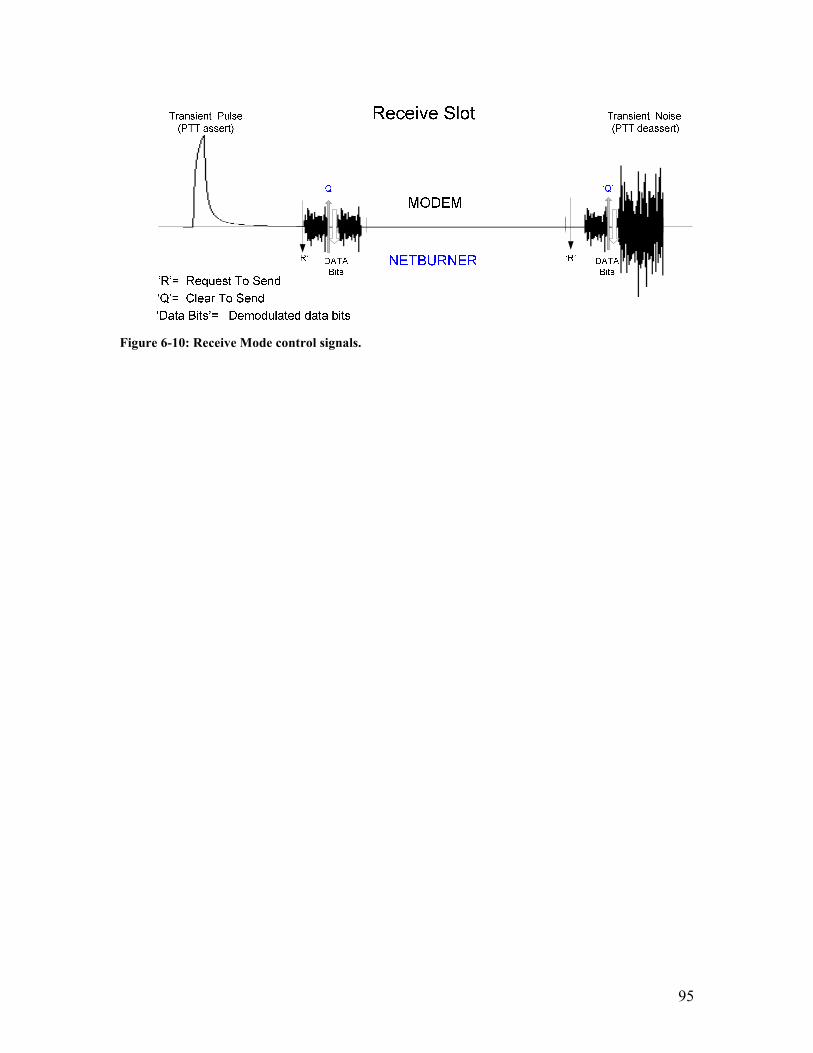
95
Figure 6-10: Receive Mode control signals.
96
7. SOFTWARE IMPLEMENTATION
Chapter 5 introduced the design and implementation of the modems and their use with
the DREAMS software. Chapter 6 described the components of the transmit and receive
slots and discussed the efficiency of transmission. This chapter discusses the
implementation of the software algorithms. The software implementation is described
only for the operations performed on the EVM. The software for implementing the
Ethernet stack on the NetBurner is beyond the scope of this thesis. This basic stack was
provided with the NetBurner, and the NetBurner application code was modified as
described in reference [30]. Section 7.2.1 introduces the main routine. The demodulator
and modulator algorithms are described in Sections 7.2.2 and 7.2.3 respectively.
7.1. Modem States
The modems have three distinct operational states as defined in Chapter 5: listen, receive
and transmit. In each state a different software routine is executed as shown in Figure
7-1. Due to the half duplex nature of the radio link, the modem never receives and
transmits at the same instant. The listen state is the default state for the modem. This is to
say that the modem is always listening for transmissions on the radio channel. During the
listen state the modem executes the main routine which is described in Section 7.2.1. The
next state is referred to as the receive state. The modem enters this state when it detects
any activity on the channel. The demodulated data bits are then transmitted to the
NetBurner. This process is augmented with the exchange of suitable handshaking codes
which ensure that the EVM and the NetBurner interact properly. During this state the
modem implements the demodulator routine described in Section 7.2.2.
The modem will enter into the transmit state only upon the assertion of two conditions:
first there should be no activity on the channel and second there should be data available
to transmit. Channel idleness is confirmed by the implementation of the MAC layer
protocol discussed in Chapter 5. In order to confirm availability of data, the handshaking
protocol detailed in Chapters 5 and 6. During the transmit state the modem executes the
modulator routine.
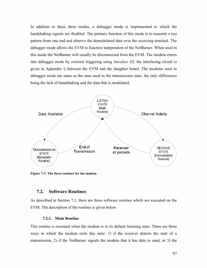
97
In addition to these three modes, a debugger mode is implemented in which the
handshaking signals are disabled. The primary function of this mode is to transmit a test
pattern from one end and observe the demodulated data over the receiving terminal. The
debugger mode allows the EVM to function independent of the NetBurner. When used in
this mode the NetBurner will usually be disconnected from the EVM. The modem enters
into debugger mode by external triggering using Interface III, the interfacing circuit is
given in Appendix I, between the EVM and the daughter board. The modules used in
debugger mode are same as the ones used in the transmission state, the only differences
being the lack of handshaking and the data that is modulated.
Figure 7-1: The three routines for the modem.
7.2. Software Routines
As described in Section 7.1, there are three software routines which are executed on the
EVM. The description of the routines is given below.
7.2.1. Main Routine
This routine is executed when the modem is in its default listening state. There are three
ways in which the modem exits this state: 1) if the receiver detects the start of a
transmission, 2) if the NetBurner signals the modem that it has data to send, or 3) the
98
debugger mode is triggered externally. In order to detect channel activity the modem
monitors the channel periodically. The periodicity is a function of the sampling rate
implemented by the codec in the EVM. For example at a sampling rate of 8 KHz the
modem monitors the channel every 125 µ secs. This is discussed in detail in Chapter 8. If
it detects any activity on the channel it will exit to the demodulator routine.
If the channel is inactive, then the modem can enter the transmit state provided there
exists data to be transmitted. To check for the availability of data, the EVM transmits the
handshaking code ‘a’ as described in Chapter 6. If the NetBurner has data, then it
proceeds by exchanging the appropriate handshaking codes. The main routine exits to the
modulator routine once these signals are exchanged. In order to enter and exit the
debugger mode external interrupts are used.
The flowchart for the Main routine is shown in Figure 7-2. The first step in the algorithm
is to check the status of the Transmit Ready (TXR) flag. Please note that the list of the
software flags used is given in Appendix H. This flag is set at the end of the backoff
algorithm. The modem will enter the backoff routine only if there is data to be
transmitted. At the same time, it also checks the status of the Interrupt Request (IRQ)
flag. If the IRQ flag is set, the main routine branches into debugger mode. Next, it checks
for activity on the channel. If any signal is detected, the main routine exits to the Receiver
routine. In the following step it checks for response to the data send request which was
made to the NetBurner by using the handshaking code ‘R’. This was described in Chapter
6. If the NetBurner has data, it sends the number of packets to be transmitted and the
main routine starts a random backoff timer and loops back to first step. When the backoff
timer expires, the TXR flag is set. The backoff algorithm is implemented by generating a
random number.
The steps are summarized below:
STEP1: Start.
STEP2: Check the status of TXR flag and IRQ flag. If set goto A (Figure 7-3 ).
STEP3: Check channel activity. If signal present goto A.
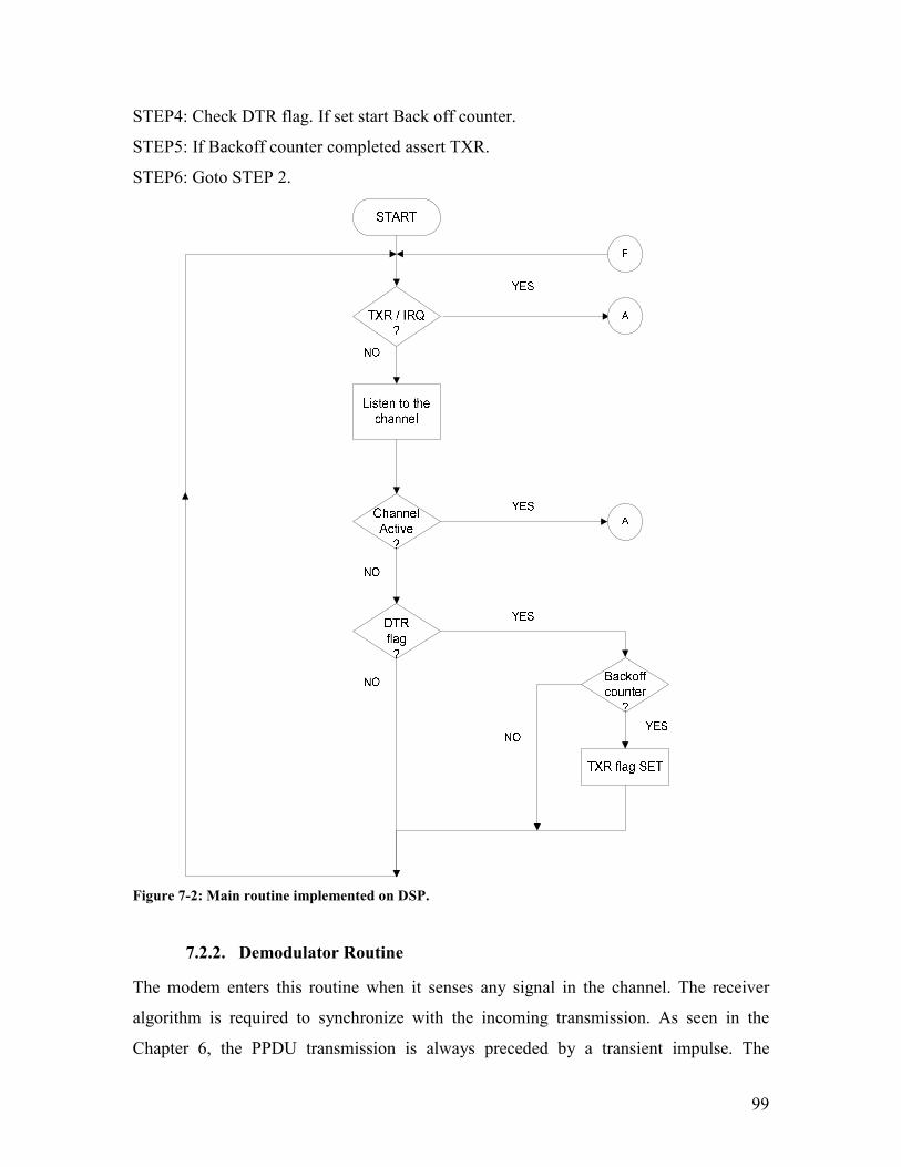
99
STEP4: Check DTR flag. If set start Back off counter.
STEP5: If Backoff counter completed assert TXR.
STEP6: Goto STEP 2.
Figure 7-2: Main routine implemented on DSP.
7.2.2. Demodulator Routine
The modem enters this routine when it senses any signal in the channel. The receiver
algorithm is required to synchronize with the incoming transmission. As seen in the
Chapter 6, the PPDU transmission is always preceded by a transient impulse. The
100
synchronization takes place in two stages. In the first stage of synchronization, the
receiver detects the impulse on the channel using the double window implementation
used in packet detection, which was described in Chapter 3. It then enters into an
RX_KEY interval in order to avoid a false alarm over the duration of transient impulse.
At the second stage of synchronization, the algorithm uses a correlator in conjunction
with the double window implementation. The correlator structure is used in symbol
symchronization which was described in Chapter 3. The double window method, which
detects the signal on the basis of signal-to-noise ratio, is used for coarse tuning.
Correlating the received signal with the local copy of the known header enables fine
tuning. Once the start of packet slot has been located, the receiver starts demodulating the
data using the modules described in Chapter 3. The demodulated data is transmitted from
the EVM over the serial port to the NetBurner. This transfer is preceded by the exchange
of receiver mode handshaking codes ‘R’ and ‘Q” which where described in Chapter 6.
This procedure is repeated for every PPDU transmission. Thus, the receive algorithm
repeats the second stage of synchronization to resynchronize each PPDU transmission.
The algorithm can be summarized as:
STEP1: Check Status of FD flag (False Detection Flag). If it is set go to B ( Figure 7-4 ).
STEP2: Wait for duration for RX_KEY interval.
STEP3: Check for status of Timeout flags. If SET goto F ( Figure 7-2).
STEP4: If signal is present, send RTS else goto STEP 3.
STEP5: Demodulated Data.
STEP6: Check for status of CTS flag. If SET, send data over serial flag else goto STEP 3.
The demodulator routine is shown in Figure 7-3. The software flags used are described in
Appendix H. Further, the demodulator routine overlaps with the duration of the receive
slot which was discussed in Chapter 6.

101
Figure 7-3:Demodulator routine implemented on DSP.

102
7.2.3. Modulator Routine
In absence of any channel activity, when the modem is in its default main routine, the
EVM periodically queries the NetBurner for data. If the NetBurner has data to send, it
responds by sending an 8-bit binary number between 0x01 to 0x0C which represents the
number of PPDUs that will be transmitted in the transmit slot, as discussed in Chapter 6.
After the initial handshaking, the main routine branches to the modulator routine at the
end of the randomly selected backoff interval. Once in the modulator routine, the modem
first asserts the PTT line to occupy the channel so that other modems will notice the
channel activity and will therefore inhibit any scheduled transmission. On receiving the
data bits from the NetBurner, the EVM modulates them to form a single PPDU. The
SymbolSentFlag (SSF), described in Appendix H, is used to communicate the
transmission of a single PPDU. At the end of a single PPDU, the EVM enters into a no-
op (no operation) stage for the duration of the Inter-PPDU Interval. This process is
repeated until the PacketSentFlag (PSF) is SET which indicates that all data bits to be
transmitted have been converted into corresponding PPDUs. Once all the PPDUs have
been transmitted, the EVM waits for the duration of the End of Transmit (EOT) interval
before PTT deassertion. In order to ensure that no false alarms are generated before the
end of PTT deassertion transient, the modem will remain in the transmit routine for the
duration of TX_UNKEY interval. The modulator routine overlaps with the transmit slot.
The make up of the transmission slot was discussed in Chapter 6. The Figure 7-4 shows
the flow chart for the modulator routine.
The algorithm can be summarized as:
STEP1: Assert the Push To Talk (PTT) signal.
STEP2: Send DTR over the serial port to obtain data from the NetBurner.
STEP3: Wait for the duration of TX_KEY interval.
STEP4: Check the status of the PSF flag. If SET goto STEP 9 else goto STEP 5.
STEP5: Check the status of the SST flag. If SET goto STEP 8 else goto STEP 6.
STEP6: Modulate the data to form the audio signal and send it to radio.
STEP7: Send DTR signal (ASCII ‘a’) to obtain data from NetBurner and goto STEP 5.

103
STEP8: Wait for the Inter-packet Interval and then transmit DTR signal (ASCII ‘a’).
Goto STEP 4.
STEP9: Wait for EOT interval.
STEP10: Send PTT deassert signal and wait for TX_UNKEY interval. Goto F.

104
Figure 7-4: Modulator routine implemented on DSP.

105
8. EXPERIMENTAL SETUP AND PERFORMANCE
EVALUATION
This Chapter discusses the frequency and time domain characteristics of the audio band
OFDM signal and the performance of the system under the conditions of Additive White
Gaussian Noise (AWGN), carrier phase incoherency and synchronization errors. In
Section 8.1, a detailed analysis of the factors which affect the available bandwidth and
achievable data rates is given. Section 8.2, lists the simulated configuration and the
associated parameters. The comparison between the performances of different
configurations is given in Section 8.3.
8.1. Factors affecting the Data Rate
The data rate for the system depends on the frequency response of the audio system in the
radio, the size of FFT/IFFT used in the implementation, the data mapping scheme
implemented and the sampling rate selected for the codec in the EVM.
8.1.1. Frequency Response
As mentioned in Chapter 1, the radio is designed to transmit voice signals. The voice
signals generally are contained in a bandwidth ranging from 300 Hz to 3.3 KHz. The
frequency response of the radio is tailored for this passband. Figure 8-1 and Figure 8-2
show the measured 3dB and 10dB bandwidths for a typical NBFM VHF radio. The radio
used to obtain the plots was an ICOM 2TH VHF radio.

106
Figure 8-1: Frequency response showing the 3dB bandwidth for the ICOM 2TH radio.
Figure 8-2: Frequency response showing the 10dB bandwidth for ICOM 2TH radio.
As seen from Figure 8-1 and Figure 8-2 the 3 dB bandwidth for the radio extends from
about 400 Hz to 3 KHz and the 10dB bandwidth for the radio approximately ranges from
300 Hz to 4.3 KHz. This roughly translates to a 3dB bandwidth of 2.7 KHz and a 10 dB
bandwidth of 4 KHz. These frequency characteristics of the radio restrict the possible
bandwidth of the baseband signal since the higher frequency subcarriers will be heavily
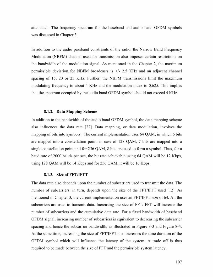
107
attenuated. The frequency spectrum for the baseband and audio band OFDM symbols
was discussed in Chapter 3.
In addition to the audio passband constraints of the radio, the Narrow Band Frequency
Modulation (NBFM) channel used for transmission also imposes certain restrictions on
the bandwidth of the modulation signal. As mentioned in the Chapter 2, the maximum
permissible deviation for NBFM broadcasts is +/- 2.5 KHz and an adjacent channel
spacing of 15, 20 or 25 KHz. Further, the NBFM transmissions limit the maximum
modulating frequency to about 4 KHz and the modulation index to 0.625. This implies
that the spectrum occupied by the audio band OFDM symbol should not exceed 4 KHz.
8.1.2. Data Mapping Scheme
In addition to the bandwidth of the audio band OFDM symbol, the data mapping scheme
also influences the data rate [22]. Data mapping, or data modulation, involves the
mapping of bits into symbols. The current implementation uses 64 QAM, in which 6 bits
are mapped into a constellation point, in case of 128 QAM, 7 bits are mapped into a
single constellation point and for 256 QAM, 8 bits are used to form a symbol. Thus, for a
baud rate of 2000 bauds per sec, the bit rate achievable using 64 QAM will be 12 Kbps,
using 128 QAM will be 14 Kbps and for 256 QAM, it will be 16 Kbps.
8.1.3. Size of FFT/IFFT
The data rate also depends upon the number of subcarriers used to transmit the data. The
number of subcarriers, in turn, depends upon the size of the FFT/IFFT used [12]. As
mentioned in Chapter 3, the current implementation uses an FFT/IFFT size of 64. All the
subcarriers are used to transmit data. Increasing the size of FFT/IFFT will increase the
number of subcarriers and the cumulative data rate. For a fixed bandwidth of baseband
OFDM signal, increasing number of subcarriers is equivalent to decreasing the subcarrier
spacing and hence the subcarrier bandwidth, as illustrated in Figure 8-3 and Figure 8-4.
At the same time, increasing the size of FFT/IFFT also increases the time duration of the
OFDM symbol which will influence the latency of the system. A trade off is thus
required to be made between the size of FFT and the permissible system latency.
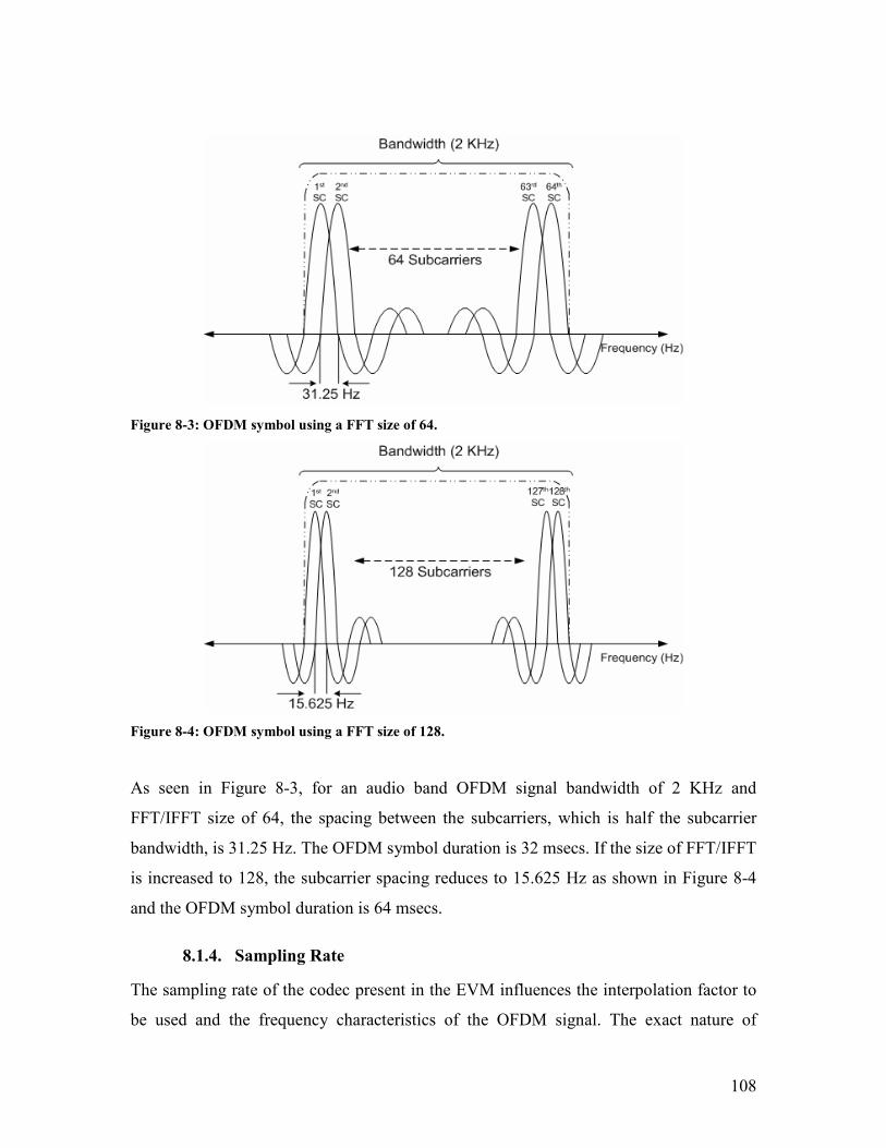
108
Figure 8-3: OFDM symbol using a FFT size of 64.
Figure 8-4: OFDM symbol using a FFT size of 128.
As seen in Figure 8-3, for an audio band OFDM signal bandwidth of 2 KHz and
FFT/IFFT size of 64, the spacing between the subcarriers, which is half the subcarrier
bandwidth, is 31.25 Hz. The OFDM symbol duration is 32 msecs. If the size of FFT/IFFT
is increased to 128, the subcarrier spacing reduces to 15.625 Hz as shown in Figure 8-4
and the OFDM symbol duration is 64 msecs.
8.1.4. Sampling Rate
The sampling rate of the codec present in the EVM influences the interpolation factor to
be used and the frequency characteristics of the OFDM signal. The exact nature of

109
influence will be discussed in Section 8.2. The codec on the EVM supports sampling
rates of 8 KHz, 12 KHz, 16 KHz, 24 KHz and 44.1 KHz. In the current implementation
the sampling rate has been fixed to 8 KHz which is equivalent to a sampling interval of
125 secµ .
8.2. Calculation of Data Rate
From the frequency response plots in Figure 8-1 and Figure 8-2 for the Icom T2H radio,
it can be observed that the 3dB bandwidth available at the radio is about 3 KHz. There
are a number of possible configurations that satisfy all the requirements described in
Section 8.1. For ease in software implementation, the size of FFT/IFFT i.e. the number of
subcarriers and length of the cyclic prefix remains same in all the configurations [32].
Thus, the number of samples representing baseband OFDM symbols is fixed to 80 as
described in Section 3.1.7. The bandwidth of the baseband OFDM symbol and the
resulting data rate is now a function of the sampling rate and the interpolation factor.
Sections 8.2.1, 8.2.2, 8.2.3 and 8.2.4 describe the various possible configurations in
detail.
8.2.1. Version 1.1
This version uses an interpolation factor of 4 and a codec sampling rate of 8 KHz. Thus,
the total number of samples representing an audio band OFDM symbol is 320 (80*4)
samples. Further, the audio band carrier frequency is represented by 4 samples per cycle.
For the codec sampling rate of 8 KHz, this translates to an audio band carrier frequency
of 2 KHz and audio band OFDM symbol duration of 40 msec. The bandwidth per
subcarrier is 31.25 Hz and the cumulative bandwidth of the subcarriers which represents
the audio band OFDM symbol bandwidth, is 2 KHz. The data rate for this version varies
depending upon the data mapping scheme used. Table 8-1 summarizes the parameters for
Version 1.1.

110
Parameters Version1.1a Version1.1b Version1.1c
Audio band Carrier
Frequency (KHz)
2 2 2
IFFT Size( number
of subcarriers)
64 64 64
Interpolation Factor 4 4 4
Subcarrier spacing
(Hz)
31.25 31.25 31.25
BW of audio band
OFDM Symbol
(KHz)
2 2 2
Lowest Carrier
Frequency (KHz)
1 1 1
Highest Carrier
Frequency (KHz)
3 3 3
Duration of audio
band OFDM Symbol
msec
32 32 32
Data Modulation 64 QAM 128 QAM 256 QAM
Data Rate Kbps 12 14 16
Sampling Frequency
(KHz)
8 8 8
Table 8-1: Configuration parameters for Version 1.1.
8.2.2. Version 1.2
This version uses an interpolation factor of 6 and the codec sampling rate of 12 KHz.
Thus the total number of samples representing the audio band OFDM symbol is 480
(80*6) samples. The audio band carrier frequency is represented by 6 samples per cycle.
For the selected codec sampling rate of 12 KHz, this translates to audio band carrier
frequency of 2 KHz and audio band OFDM symbol duration of 40 msec. The bandwidth
per subcarrier is 31.25 Hz and the cumulative bandwidth of the subcarriers which
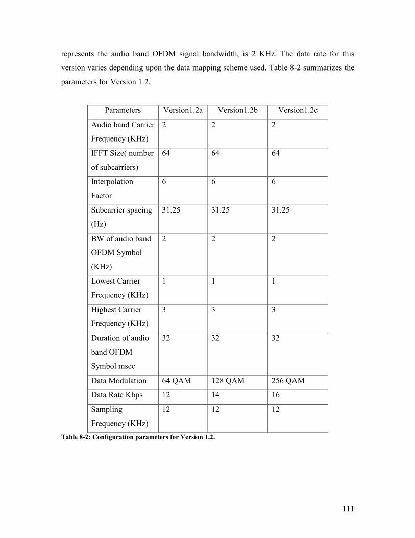
111
represents the audio band OFDM signal bandwidth, is 2 KHz. The data rate for this
version varies depending upon the data mapping scheme used. Table 8-2 summarizes the
parameters for Version 1.2.
Parameters Version1.2a Version1.2b Version1.2c
Audio band Carrier
Frequency (KHz)
2 2 2
IFFT Size( number
of subcarriers)
64 64 64
Interpolation
Factor
6 6 6
Subcarrier spacing
(Hz)
31.25 31.25 31.25
BW of audio band
OFDM Symbol
(KHz)
2 2 2
Lowest Carrier
Frequency (KHz)
1 1 1
Highest Carrier
Frequency (KHz)
3 3 3
Duration of audio
band OFDM
Symbol msec
32 32 32
Data Modulation 64 QAM 128 QAM 256 QAM
Data Rate Kbps 12 14 16
Sampling
Frequency (KHz)
12 12 12
Table 8-2: Configuration parameters for Version 1.2.

112
8.2.3. Version 2
The bandwidth of the audio band OFDM symbol for this version is 3 KHz. The
interpolation factor used is 5 and the codec sampling rate selected is 12 KHz. Thus the
total number of samples representing the audio band OFDM symbol is 400 (80*5)
samples. The audio band carrier frequency is represented by 5 samples per cycle which
equates to an audio band carrier frequency of 2.4 KHz. The duration of an audio band
OFDM symbol is 26.67 msec. The bandwidth per subcarrier is 46.87 Hz and the
cumulative bandwidth of the subcarriers is 3 KHz. The data rate for this version varies
depending upon the data mapping scheme used. Table 8-3 gives further details on
Version 2.
Parameters Version2a Version2b Version2c
Audio band Carrier
Frequency (KHz)
2.4 2.4 2.4
IFFT Size( number
of subcarriers)
64 64 64
Interpolation
Factor
5 5 5
Subcarrier spacing
(Hz)
46.87 46.87 46.87
BW of audio band
OFDM Symbol
(KHz)
3 3 3
Lowest Carrier
Frequency (KHz)
0.9 0.9 0.9
Highest Carrier
Frequency (KHz)
3.9 3.9 3.9
Duration of audio
band OFDM
Symbol msec
21.33 21.33 21.33
Data Modulation 64 QAM 128 QAM 256 QAM

113
Data Rate Kbps 18 21 24
Sampling
Frequency (KHz)
12 12 12
Table 8-3: Configuration parameters for Version 2.
8.2.4. Version 3
The bandwidth of the audio band OFDM symbol is 4 KHz which represents the
approximate 10dB bandwidth of the audio passband. The interpolation factor used is 6
and the codec sampling rate is 16 KHz. Thus, the total number of samples representing
the audio band OFDM signal is 480 (80*6) samples. The audio band carrier frequency is
represented by 6 samples per cycle. This translates to an audio band carrier frequency of
2.67 KHz and audio band OFDM symbol duration of 20 msec. The bandwidth per
subcarrier is 62 Hz and thus the cumulative bandwidth of the subcarriers is 4 KHz. The
data rate for this version varies depending upon the data mapping scheme used as seen in
Table 8-4.
Parameters Version3a Version3b Version3c
Audio band Carrier
Frequency (KHz)
2.67 2.67 2.67
IFFT Size( number
of subcarriers)
64 64 64
Interpolation
Factor
6 6 6
Subcarrier spacing
(Hz)
62.5 62.5 62.5
BW of audio band
OFDM Symbol
(KHz)
4 4 4
Lowest Carrier
Frequency (KHz)
0.667 0.667 0.667

114
Highest Carrier
Frequency (KHz)
4.667 4.667 4.667
Duration of audio
band OFDM
Symbol msec
16 16 16
Data Modulation 64 QAM 128 QAM 256 QAM
Data Rate Kbps 24 28 32
Sampling
Frequency (KHz)
16 16 16
Table 8-4: Configuration parameters for Version 3.
8.3. Performance Evaluation using Simulation
This section investigates the performances of all the versions in terms of their respective
Bit Error Rates (BER). Section 8.3.1 explores the performance in presence of Additive
White Gaussian Noise (AWGN). In addition to AWGN, the performance of the
demodulator is also contingent upon the phase coherency of the audio band carrier; this
issue is elaborated in Section 8.3.2. The degradation in performance due to
synchronization errors is discussed in Section 8.3.3. All the evaluations have been
performed using MATLAB®. The audio passband of the radio is emulated by a filter
having the frequency response and phase response shown in Figure 8-5. The filter has a 3
dB passband between 300 Hz to 3500 Hz which translates to a 3dB bandwidth of 3.3
KHz and a 10 dB passband between 200 Hz to 4200 Hz which translates to a 10 dB
bandwidth of 4 KHz. The filter also has a linear phase response in the frequency range of
interest.
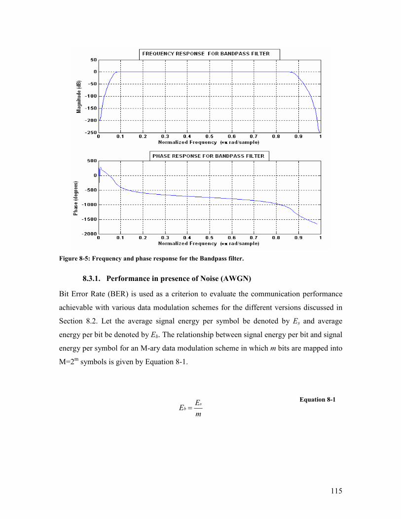
115
Figure 8-5: Frequency and phase response for the Bandpass filter.
8.3.1. Performance in presence of Noise (AWGN)
Bit Error Rate (BER) is used as a criterion to evaluate the communication performance
achievable with various data modulation schemes for the different versions discussed in
Section 8.2. Let the average signal energy per symbol be denoted by Es and average
energy per bit be denoted by Eb. The relationship between signal energy per bit and signal
energy per symbol for an M-ary data modulation scheme in which m bits are mapped into
M=2m symbols is given by Equation 8-1.
m
EE
sb =
Equation 8-1
116
where
Eb = Energy per bit
Es = Energy per symbol
M = Number of symbols
A similar relationship exists for the signal to noise (SNR) ratio per bit and signal to noise
(SNR) per symbol [22].
m
sbγ
γ =
Equation 8-2
where
bγ = SNR per bit
sγ = SNR per symbol
M = Number of symbols
The acceptable value for Bit Error Rate (BER) depends upon the application. Some
voice-band modem applications, such as the ones which are responsible for the transfer of
financial data permit error rates no greater than 10-5. In the case of applications like
digitized voice in a cellular or mobile radio system, the tolerable error rates can be as
high as 10-2 to 10
-3. For high fidelity audio systems like CD players, the acceptable BER
performance is on the order of 10-8. The BER performance is affected by the SNR of the
received signal. The SNR level at the demodulator depends upon a number of factors like
received power, distance from transmitter, transmitted power and the surrounding terrain.
The relationship between transmitted and received powers in a single path free-space
channel is given by Equation 8-2 [31].
2r)
4(
P
dGG
Prt
t πλ
=
Equation 8-3

117
where
Pr = Received power.
Pt = Transmitted power.
Gt = Gain at the transmitter antenna
Gr = Gain at the receiver antenna
λ = wavelength of the transmitted signal
D = distance between the transmitter and
receiver
Using Equation 8-3, a path loss model can be developed which gives the difference in the
transmitted power and received power as a function of the distance and the frequency of
transmission. This is referred to as the free-space path loss equation and is given by
Equation 8-4.
)log(20)log(204.32)( fddBLp ++=
Equation 8-4
where
Lp = Path loss in dB
D = Distance in kilometers
F = Frequency of transmission in MHz
Figure 8-6 shows the relationship between the signal to noise ratio and the distance from
the transmitter. The transmitter power, Pt, varies from 1W, 2W, 4W, 6W. The transmit
frequency is assumed to be 150 MHz. The received power, Pr, is calculated as shown in
Equation 8-5.
pt LPdB −=)(Pr
Equation 8-5
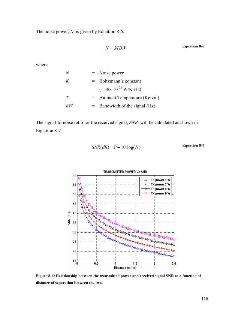
118
The noise power, N, is given by Equation 8-6.
kTBWN =
Equation 8-6
where
N = Noise power
K = Boltzmann’s constant
(1.38x 10⁻²³ W/K-Hz)
T = Ambient Temperature (Kelvin)
BW = Bandwidth of the signal (Hz)
The signal-to-noise ratio for the received signal, SNR, will be calculated as shown in
Equation 8-7.
)log(.10P)( r NdBSNR −=
Equation 8-7
Figure 8-6: Relationship between the transmitted power and received signal SNR as a function of
distance of separation between the two.

119
In the case of analog communications, SNR is often used as a performance criterion as
opposed to BER. Analog mobile radio systems typically require an SNR of at least 18
dB. High fidelity FM broadcasting systems require an SNR of at least 30 dB [21].
The BER requirement for a system is driven by the nature of data traffic it is required to
communicate. As discussed in Chapter 4, the current system uses UDP/IP packets to
transfer data. The maximum size for the UDP/IP packet is 1472 bytes. Thus in order to
have a system which can transfer the maximum UDP/IP packet sizes, the permissible
BER should be in the vicinity of 10-5. This way an UDP/IP packet of any legitimate
length can be guaranteed to be delivered. The theoretical limit on the symbol error
probability for different values of SNR can be approximated by Equation 8-8 [22].
])1(
3[)
11(4
NM
EQ
MP
ss
−−=
Equation 8-8
where
Ps = Noise power
M = Boltzmann’s constant
(1.38x 10⁻²³ W/K-Hz)
E = Ambient Temperature (Kelvin)
BW = Bandwidth of the signal (Hz)
Using Equation 8-8, the approximate SNR required for obtaining BER of 10-5 using 64
QAM is 26 dB, for 128 QAM it is 29dB and for 256 QAM it is 33 dB. Figure 8-7 shows
the theoretical limits on performance of 64 QAM, 128 QAM and 256 QAM.

120
Figure 8-7: Theoretical limits on BER performances of 64 QAM, 128 QAM, 256 QAM.
The performances of the different configurations in presence of AWGN are shown in
Figure 8-8 and Figure 8-9.
(a)
(b)
Figure 8-8: Performance of the demodulator in presence of AWGN for (a) 64 QAM Modulation and
(b) 128 QAM Modulation.
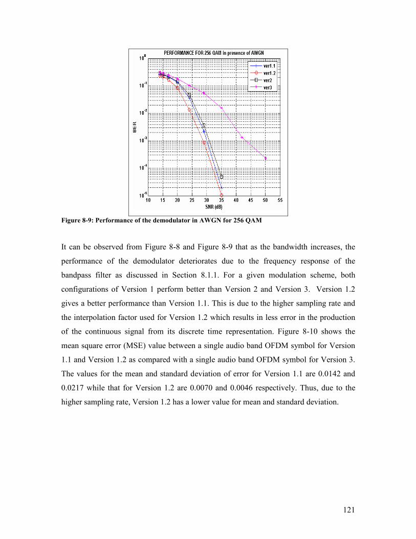
121
Figure 8-9: Performance of the demodulator in AWGN for 256 QAM
It can be observed from Figure 8-8 and Figure 8-9 that as the bandwidth increases, the
performance of the demodulator deteriorates due to the frequency response of the
bandpass filter as discussed in Section 8.1.1. For a given modulation scheme, both
configurations of Version 1 perform better than Version 2 and Version 3. Version 1.2
gives a better performance than Version 1.1. This is due to the higher sampling rate and
the interpolation factor used for Version 1.2 which results in less error in the production
of the continuous signal from its discrete time representation. Figure 8-10 shows the
mean square error (MSE) value between a single audio band OFDM symbol for Version
1.1 and Version 1.2 as compared with a single audio band OFDM symbol for Version 3.
The values for the mean and standard deviation of error for Version 1.1 are 0.0142 and
0.0217 while that for Version 1.2 are 0.0070 and 0.0046 respectively. Thus, due to the
higher sampling rate, Version 1.2 has a lower value for mean and standard deviation.
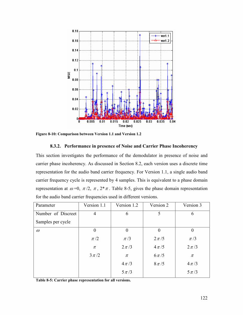
122
Figure 8-10: Comparison between Version 1.1 and Version 1.2
8.3.2. Performance in presence of Noise and Carrier Phase Incoherency
This section investigates the performance of the demodulator in presence of noise and
carrier phase incoherency. As discussed in Section 8.2, each version uses a discrete time
representation for the audio band carrier frequency. For Version 1.1, a single audio band
carrier frequency cycle is represented by 4 samples. This is equivalent to a phase domain
representation at ω =0, π /2, π , 2*π . Table 8-5, gives the phase domain representation
for the audio band carrier frequencies used in different versions.
Parameter Version 1.1 Version 1.2 Version 2 Version 3
Number of Discreet
Samples per cycle
4 6 5 6
ω 0
π /2
π
3π /2
0
π /3
2π /3
π
4π /3
5π /3
0
2π /5
4π /5
6π /5
8π /5
0
π /3
2π /3
π
4π /3
5π /3
Table 8-5: Carrier phase representation for all versions.
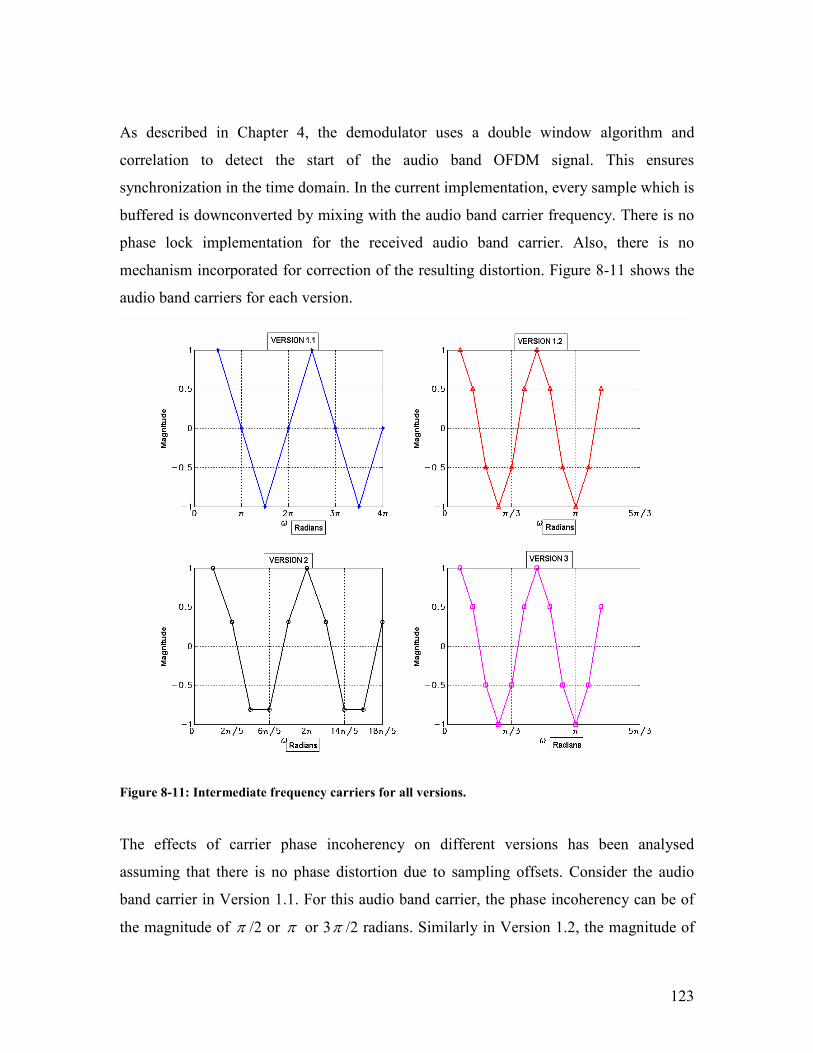
123
As described in Chapter 4, the demodulator uses a double window algorithm and
correlation to detect the start of the audio band OFDM signal. This ensures
synchronization in the time domain. In the current implementation, every sample which is
buffered is downconverted by mixing with the audio band carrier frequency. There is no
phase lock implementation for the received audio band carrier. Also, there is no
mechanism incorporated for correction of the resulting distortion. Figure 8-11 shows the
audio band carriers for each version.
Figure 8-11: Intermediate frequency carriers for all versions.
The effects of carrier phase incoherency on different versions has been analysed
assuming that there is no phase distortion due to sampling offsets. Consider the audio
band carrier in Version 1.1. For this audio band carrier, the phase incoherency can be of
the magnitude of π /2 or π or 3π /2 radians. Similarly in Version 1.2, the magnitude of
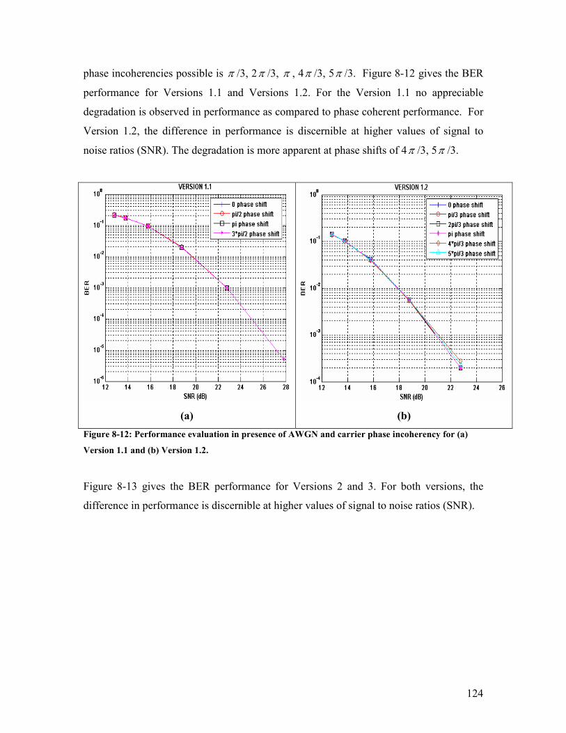
124
phase incoherencies possible is π /3, 2π /3, π , 4π /3, 5π /3. Figure 8-12 gives the BER
performance for Versions 1.1 and Versions 1.2. For the Version 1.1 no appreciable
degradation is observed in performance as compared to phase coherent performance. For
Version 1.2, the difference in performance is discernible at higher values of signal to
noise ratios (SNR). The degradation is more apparent at phase shifts of 4π /3, 5π /3.
(a)
(b)
Figure 8-12: Performance evaluation in presence of AWGN and carrier phase incoherency for (a)
Version 1.1 and (b) Version 1.2.
Figure 8-13 gives the BER performance for Versions 2 and 3. For both versions, the
difference in performance is discernible at higher values of signal to noise ratios (SNR).
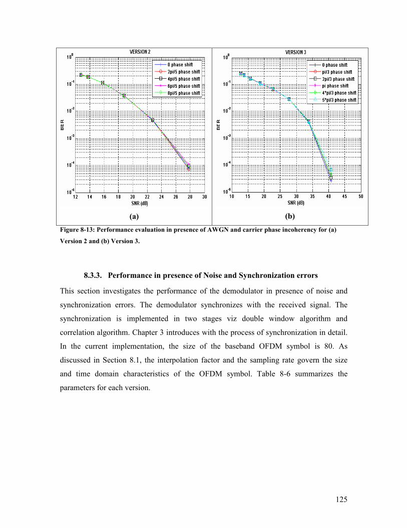
125
(a)
(b)
Figure 8-13: Performance evaluation in presence of AWGN and carrier phase incoherency for (a)
Version 2 and (b) Version 3.
8.3.3. Performance in presence of Noise and Synchronization errors
This section investigates the performance of the demodulator in presence of noise and
synchronization errors. The demodulator synchronizes with the received signal. The
synchronization is implemented in two stages viz double window algorithm and
correlation algorithm. Chapter 3 introduces with the process of synchronization in detail.
In the current implementation, the size of the baseband OFDM symbol is 80. As
discussed in Section 8.1, the interpolation factor and the sampling rate govern the size
and time domain characteristics of the OFDM symbol. Table 8-6 summarizes the
parameters for each version.
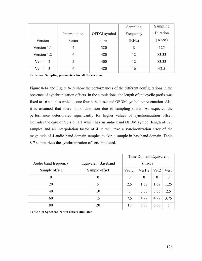
126
Version
Interpolation
Factor
OFDM symbol
size
Sampling
Frequency
(KHz)
Sampling
Duration
( secµ )
Version 1.1 4 320 8 125
Version 1.2 6 480 12 83.33
Version 2 5 400 12 83.33
Version 3 6 480 16 62.5
Table 8-6: Sampling parameters for all the versions.
Figure 8-14 and Figure 8-15 show the performances of the different configurations in the
presence of synchronization offsets. In the simulations, the length of the cyclic prefix was
fixed to 16 samples which is one fourth the baseband OFDM symbol representation. Also
it is assumed that there is no distortion due to sampling offset. As expected the
performance deteriorates significantly for higher values of synchronization offset.
Consider the case of Version 1.1 which has an audio band OFDM symbol length of 320
samples and an interpolation factor of 4. It will take a synchronization error of the
magnitude of 4 audio band domain samples to skip a sample in baseband domain. Table
8-7 summarizes the synchronization offsets simulated.
Time Domain Equivalent
(msecs) Audio band frequency
Sample offset
Equivalent Baseband
Sample offset Ver1.1 Ver1.2 Ver2 Ver3
0 0 0 0 0 0
20 5 2.5 1.67 1.67 1.25
40 10 5 3.33 3.33 2.5
60 15 7.5 4.99 4.99 3.75
80 20 10 6.66 6.66 5
Table 8-7: Synchronization offsets simulated.

127
(a)
(b)
Figure 8-14: Performance evaluation in the presence of AWGN and synchronization offsets for (a)
Version 1.1 and (b) Version 1.2.
(a)
(b)
Figure 8-15: Performance evaluation in the presence of AWGN and synchronization offsets for (a)
Version 2 and (b) Version 3.

128
8.4. Performance evaluation using prototype modem
Figure 8-16 shows the final prototype of OFDM Modem and the test setup for outdoor
testing. The objectives of these tests were to obtain a rough estimate of the modem
performance. As described in Chapter 1, the modems use Ethernet connection to transfer
the data to the final source and destination (DTE). One of the ways to evaluate
performance of modems will be to measure the packet loss rate of the system. Measuring
the packet loss, however does not give a true measure of BER performance. This is
because a single bit error or multiple bit errors may be responsible for the packet being
corrupted. This discrepancy between packet loss and BER can be minimized by keeping
the size of each UDP/IP packet as small as possible. Figure 8-17 (b) shows the java
server application used to send packets to the modem. Figure 8-17 (a) shows the java
client application which is used at receiving modem. It counts the number of packets
received. Calculating the ratio between numbers of packets sent and received gives the
percentage packet loss.
Figure 8-16: OBITS modem test bed.

129
(a)
(b)
Figure 8-17: Performance measure software, (a) client (b) server.
Figure 8-18, shows the relationship between percentage packet loss and SNR. Different
SNR values were obtained using the output attenuator of the codec on EVM, as opposed
to the use of the volume control on the radio. Using the codec on EVM gives a better
control over the SNR. It can be seen from Figure 8-1 that the percentage of packet loss
decreases as signal to noise ratio increases. The packets transmitted, used UDP/IP format
and data payload for each packet was restricted to 10 bytes. Table 8-8 tabulates the
results obtained.

130
Figure 8-18: Packet loss.
SNR (dB)
% Packets Lost Maximum BER Minimum BER
24 13.5 1.3e-1 1.6e-3
26 6.55 6.5e-2 8.18e-4
28 0.55 5.5e-3 6.875e-5
30 0.05 5e-4 6.25e-6
Table 8-8: Packet loss Vs SNR.
The maximum BER seen in Table 8-8 is calculated assuming all the bits in the lost packet
were corrupted and the minimum BER is calculated assuming only one error bit per
packet lost.
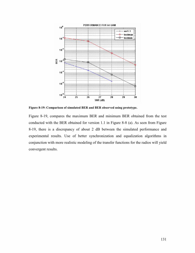
131
Figure 8-19: Comparison of simulated BER and BER observed using prototype.
Figure 8-19, compares the maximum BER and minimum BER obtained from the test
conducted with the BER obtained for version 1.1 in Figure 8-8 (a). As seen from Figure
8-19, there is a discrepancy of about 2 dB between the simulated performance and
experimental results. Use of better synchronization and equalization algorithms in
conjunction with more realistic modeling of the transfer functions for the radios will yield
convergent results.
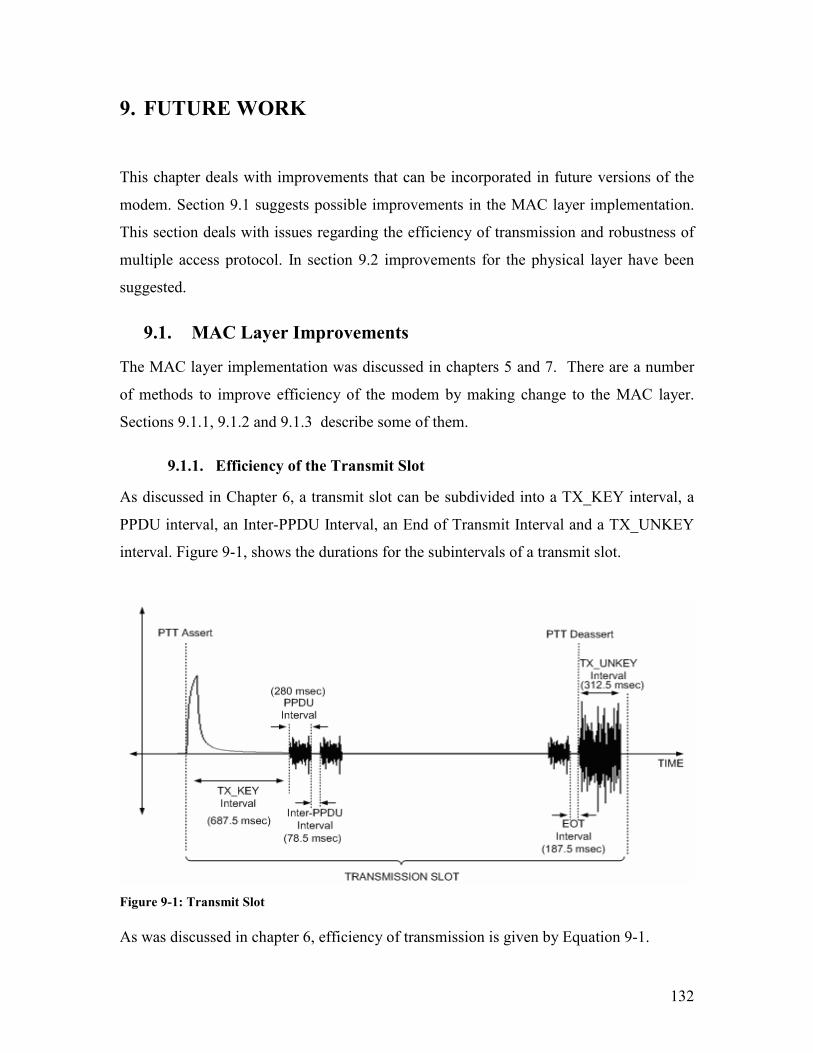
132
9. FUTURE WORK
This chapter deals with improvements that can be incorporated in future versions of the
modem. Section 9.1 suggests possible improvements in the MAC layer implementation.
This section deals with issues regarding the efficiency of transmission and robustness of
multiple access protocol. In section 9.2 improvements for the physical layer have been
suggested.
9.1. MAC Layer Improvements
The MAC layer implementation was discussed in chapters 5 and 7. There are a number
of methods to improve efficiency of the modem by making change to the MAC layer.
Sections 9.1.1, 9.1.2 and 9.1.3 describe some of them.
9.1.1. Efficiency of the Transmit Slot
As discussed in Chapter 6, a transmit slot can be subdivided into a TX_KEY interval, a
PPDU interval, an Inter-PPDU Interval, an End of Transmit Interval and a TX_UNKEY
interval. Figure 9-1, shows the durations for the subintervals of a transmit slot.
Figure 9-1: Transmit Slot
As was discussed in chapter 6, efficiency of transmission is given by Equation 9-1.
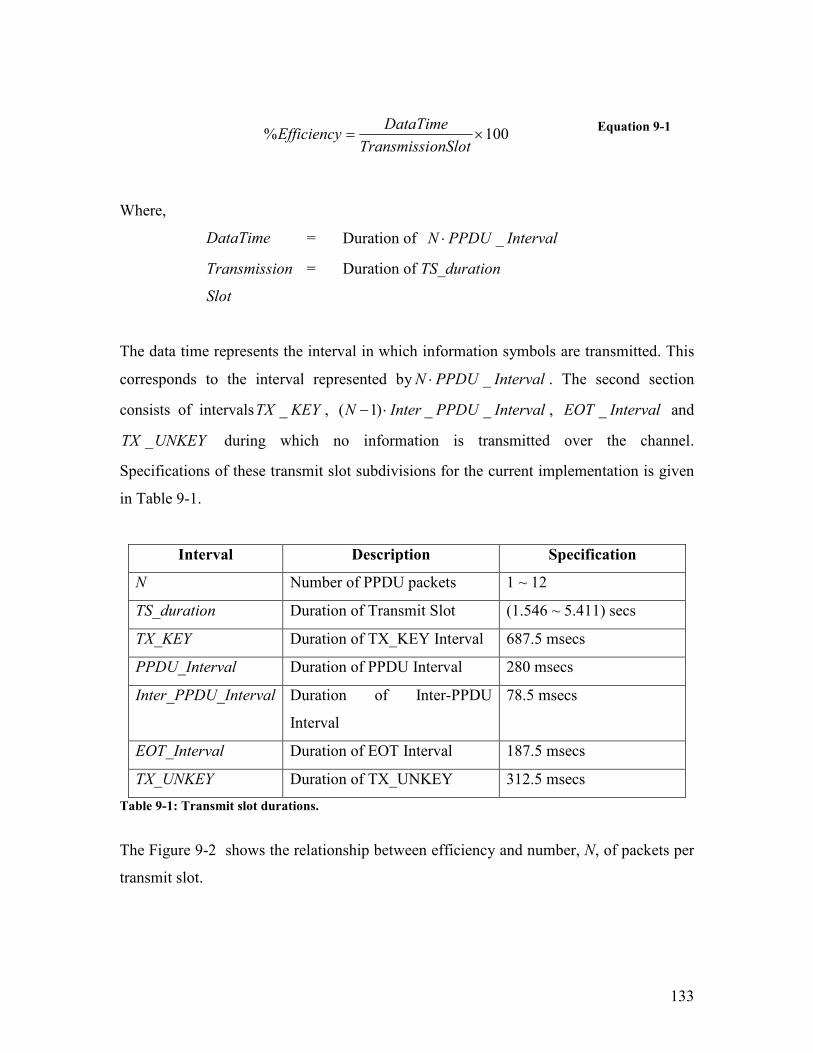
133
100% ×=onSlotTransmissi
DataTimeEfficiency
Equation 9-1
Where,
DataTime = Duration of IntervalPPDUN _⋅
Transmission
Slot
= Duration of TS_duration
The data time represents the interval in which information symbols are transmitted. This
corresponds to the interval represented by IntervalPPDUN _⋅ . The second section
consists of intervals KEYTX _ , IntervalPPDUInterN __)1( ⋅− , IntervalEOT _ and
UNKEYTX _ during which no information is transmitted over the channel.
Specifications of these transmit slot subdivisions for the current implementation is given
in Table 9-1.
Interval Description Specification
N Number of PPDU packets 1 ~ 12
TS_duration Duration of Transmit Slot (1.546 ~ 5.411) secs
TX_KEY Duration of TX_KEY Interval 687.5 msecs
PPDU_Interval Duration of PPDU Interval 280 msecs
Inter_PPDU_Interval Duration of Inter-PPDU
Interval
78.5 msecs
EOT_Interval Duration of EOT Interval 187.5 msecs
TX_UNKEY Duration of TX_UNKEY 312.5 msecs
Table 9-1: Transmit slot durations.
The Figure 9-2 shows the relationship between efficiency and number, N, of packets per
transmit slot.
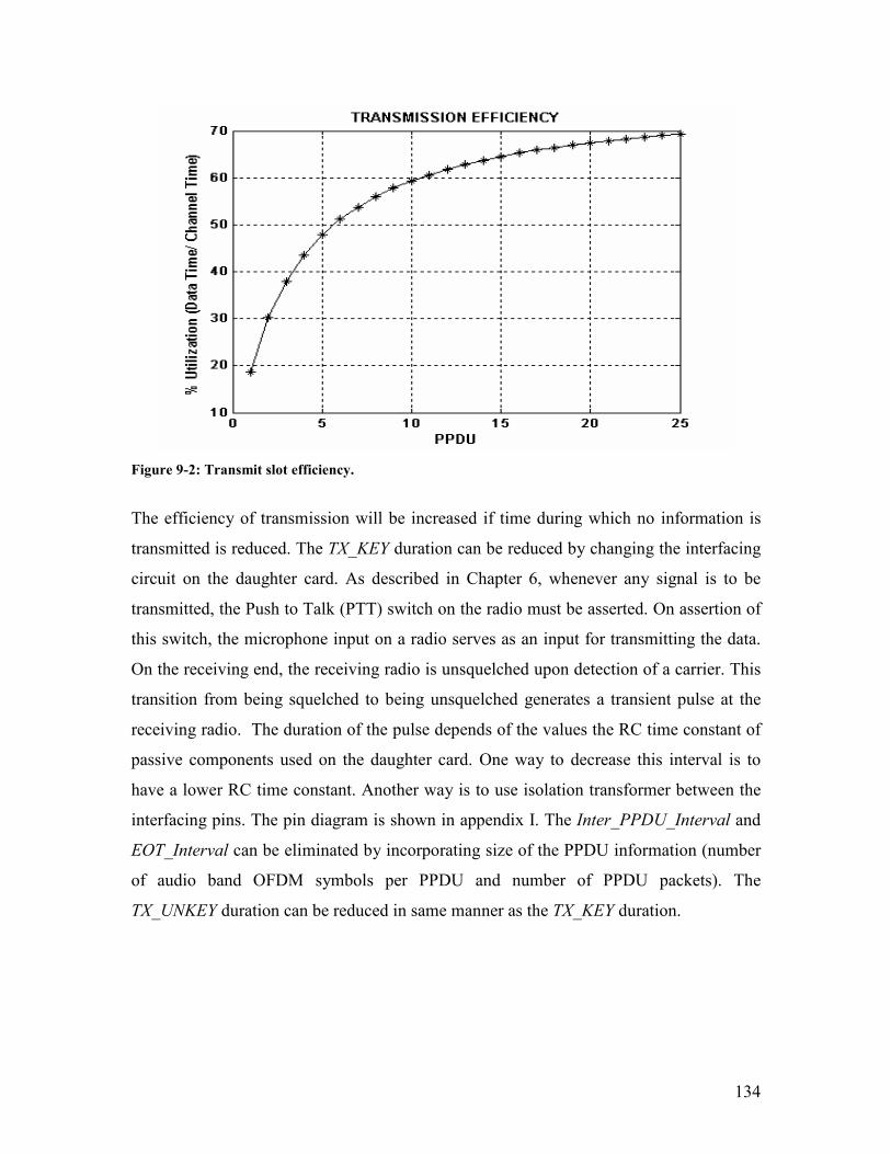
134
Figure 9-2: Transmit slot efficiency.
The efficiency of transmission will be increased if time during which no information is
transmitted is reduced. The TX_KEY duration can be reduced by changing the interfacing
circuit on the daughter card. As described in Chapter 6, whenever any signal is to be
transmitted, the Push to Talk (PTT) switch on the radio must be asserted. On assertion of
this switch, the microphone input on a radio serves as an input for transmitting the data.
On the receiving end, the receiving radio is unsquelched upon detection of a carrier. This
transition from being squelched to being unsquelched generates a transient pulse at the
receiving radio. The duration of the pulse depends of the values the RC time constant of
passive components used on the daughter card. One way to decrease this interval is to
have a lower RC time constant. Another way is to use isolation transformer between the
interfacing pins. The pin diagram is shown in appendix I. The Inter_PPDU_Interval and
EOT_Interval can be eliminated by incorporating size of the PPDU information (number
of audio band OFDM symbols per PPDU and number of PPDU packets). The
TX_UNKEY duration can be reduced in same manner as the TX_KEY duration.
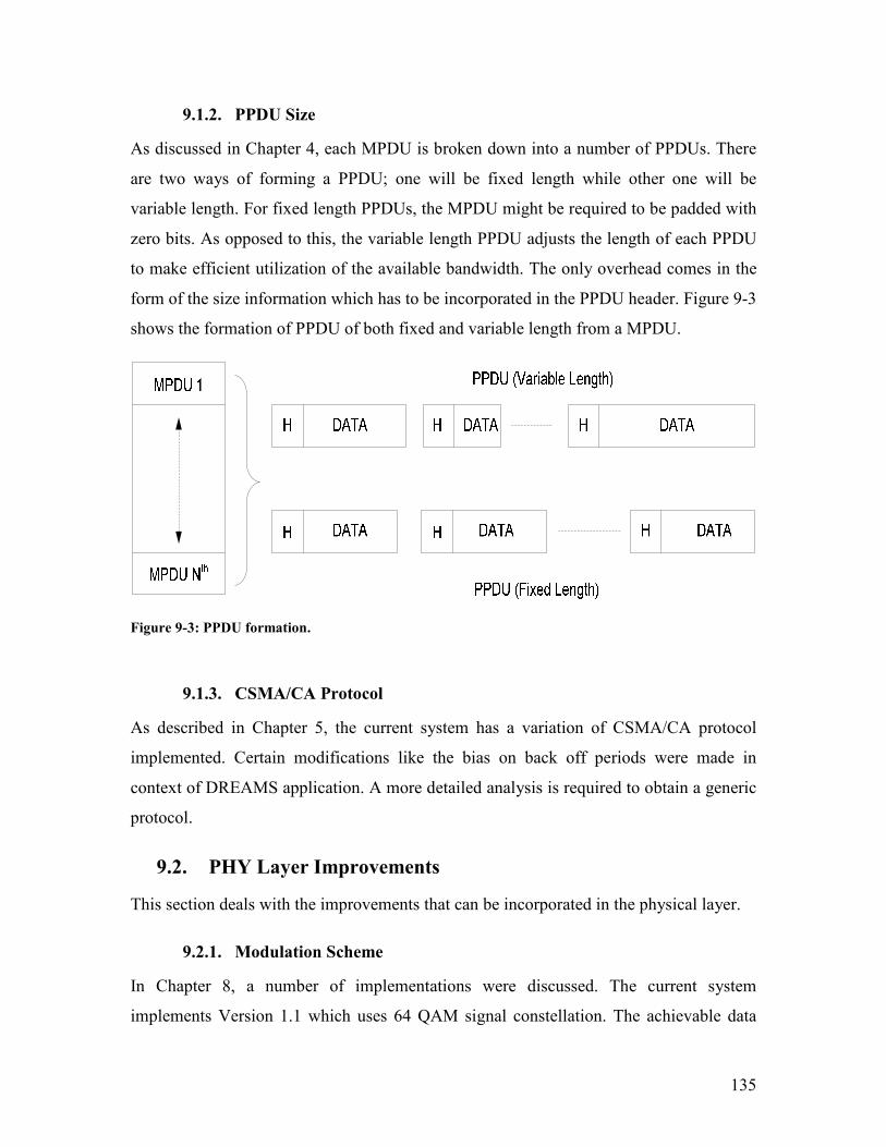
135
9.1.2. PPDU Size
As discussed in Chapter 4, each MPDU is broken down into a number of PPDUs. There
are two ways of forming a PPDU; one will be fixed length while other one will be
variable length. For fixed length PPDUs, the MPDU might be required to be padded with
zero bits. As opposed to this, the variable length PPDU adjusts the length of each PPDU
to make efficient utilization of the available bandwidth. The only overhead comes in the
form of the size information which has to be incorporated in the PPDU header. Figure 9-3
shows the formation of PPDU of both fixed and variable length from a MPDU.
Figure 9-3: PPDU formation.
9.1.3. CSMA/CA Protocol
As described in Chapter 5, the current system has a variation of CSMA/CA protocol
implemented. Certain modifications like the bias on back off periods were made in
context of DREAMS application. A more detailed analysis is required to obtain a generic
protocol.
9.2. PHY Layer Improvements
This section deals with the improvements that can be incorporated in the physical layer.
9.2.1. Modulation Scheme
In Chapter 8, a number of implementations were discussed. The current system
implements Version 1.1 which uses 64 QAM signal constellation. The achievable data

136
rate for this version stands at 12 kbps and the throughput achievable of the radio link is
about 3 kbps. The throughput calculation includes the transmit slot efficiency,
modulation scheme implemented and the encoding. Using higher modulation schemes
like 128 or 256 will increase the achievable data rate and hence the throughput.
9.2.2. Coding Techniques
All the versions discussed in Chapter 8 use convolutional encoding with an encoding rate
of ½. Different encoding formats like rate punctured convolutional encoding and block
coding need to be tested to optimize the modem performance.
9.2.3. Filter Implementation
As described in Chapter 3, the current system requires interpolation of baseband signal.
The two methods commonly implemented are zero-hold and zero-insert interpolation
which were described in Chapter 4. A low pass FIR filter is used to perform interpolation.
The delay associated with a FIR filter causes phase distortion of the filtered signal. One
of the ways to resolve this issue is to implement zero- phase distortion FIR filtered. The
required modification and the tradeoff involved need to be explored in future.
9.2.4. Peak to Average ratio (PAR ) for audio band OFDM signal
The bandwidth of FM signal depends on the modulation index. As described in Chapter
2, modulation index, β is given by Equation 9-2.
m
f
f
∆=β
Equation 9-2
where
f∆ = Deviation (Hz)
fm = Maximum modulating frequency
The deviation, f∆ , depends upon amplitude of the modulating signal. Thus the amplitude
of the generated OFDM signal will influence the bandwidth of the FM signal and hence
the performance of the modem. This issue needs to be researched further.

137
10. APPENDIX A
This appendix introduces the different peripherals and modules of the EVM which are
used in executing the software algorithms described in the Chapter 7. The Enhanced
Synchronous Serial Interface (ESSI) is used to interface the radio and codec and forms a
part of Interface III, as described in Chapter 4. In order to facilitate communication over
the serial port, the Serial Communication Interface (SCI) is used. Port D, a General
purpose Input/Output (GPIO) port is used to perform ancillary functions like PTT
assertion. The next sections will explain in detail the working of peripherals and modules
used. The peripherals used are shown in Figure 10-1.
Figure 10-1: Peripherals
1] Serial Communication Interface (SCI):
The DSP 56L307 EVM provides a full duplex port for serial communication with other
DSPs, microprocessors, or peripherals such as modems. It supports both synchronous and
asynchronous modes of operation. It can be configured for a range of baud rates and can
be used in conjunction with an external clock source or an internal clock. For the current
system, the SCI interface works at 38.4Kbps, in 10 bit asynchronous mode and has its
138
baud rate derived from an internal clock. The functioning of the SCI interface is dictated
by the contents of SCI Control Register (SCR) and SCI Clock Control Registers (SCCR).
The serial interface is interrupt driven.
2] Enhanced Synchronous Serial Interface (ESSI):
The ESSI interface provides a full-duplex serial port for serial communication with a
variety of devices including the codecs. There are two ESSI interfaces available on the
DSP. For the selected EVM, the interfaces ESSI0 and ESSI1, are both interfaced with a
stereo codec. The codec is connected to the VHF radio through an interfacing circuit
described in Appendix I. The codec functions in full duplex mode and has two stereo
channels, one representing codec_input and the other codec_output. The mode
of operation for the ESSI interfaces is selected by programming the ESSI Control
Register A (CRA) and ESSI Control Register B (CRB). This interface is interrupt driven.
The frequency of interrupts depends on the sampling frequency which, for the current
implementation, is 8 KHz. The interrupt service routine is executed twice at each
sampling time, once for the Right channel and once for the Left.
3] General Purpose Input/Output (GPIO) Ports:
There are four GPIO ports available on the EVM. Each port has a set of bidirectional
signals which can be configured as GPIO signals or as peripheral dedicated signals. For
the current system, Port E is used for the serial interface, Port C is used for the ESSI
interface and Port D provides the ancillary signaling required for interfacing the VHF
radio. Two pins of Port D are used to drive two LEDs which indicate the amplitude of
received signals. The third pin is used for assertion of PTT switch. In order to use the
Ports in GPIO mode, Port Control Register (PxRD), Port Direction Register (PxRD), and
Port GPIO Data Register (PxRD) have to be programmed with appropriate values.
4] Timer Modules:
The EVM has three internal timer modules. Each timer has a single signal which can be
configured as a bidirectional GPIO signal or as a timer signal. The timers can function as

139
watchdog timers, pulse-width modulators or can be used as event counters. In the timer
mode, the timer generates an internal interrupt when a counter value is reached. The
functioning of the timer modules depends on the contents of the Timer Control/Status
Register (TCSR), Timer Load Register (TLR), Timer Compare register (TCPR). The
current implementation uses timer modules 1 and 2 in the default timer mode. Both the
timer modules generate interrupt. Timer module 1 is programmed to generate an interrupt
every 131.25 msecs and Timer module 2 every 656.25 msecs.
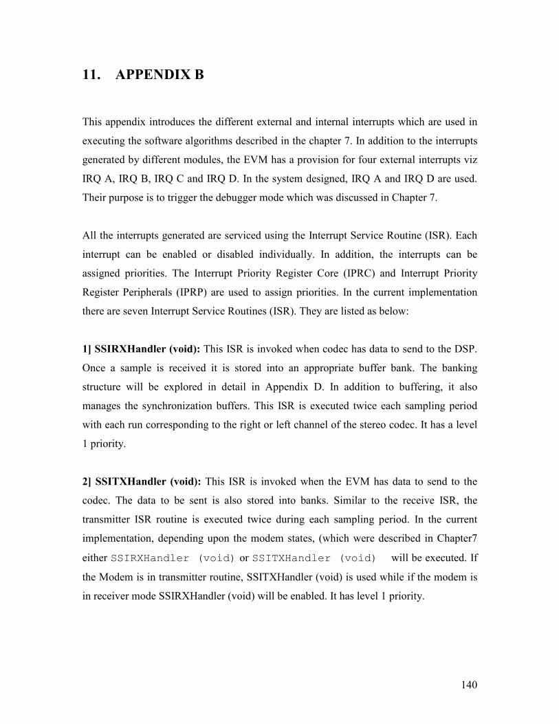
140
11. APPENDIX B
This appendix introduces the different external and internal interrupts which are used in
executing the software algorithms described in the chapter 7. In addition to the interrupts
generated by different modules, the EVM has a provision for four external interrupts viz
IRQ A, IRQ B, IRQ C and IRQ D. In the system designed, IRQ A and IRQ D are used.
Their purpose is to trigger the debugger mode which was discussed in Chapter 7.
All the interrupts generated are serviced using the Interrupt Service Routine (ISR). Each
interrupt can be enabled or disabled individually. In addition, the interrupts can be
assigned priorities. The Interrupt Priority Register Core (IPRC) and Interrupt Priority
Register Peripherals (IPRP) are used to assign priorities. In the current implementation
there are seven Interrupt Service Routines (ISR). They are listed as below:
1] SSIRXHandler (void): This ISR is invoked when codec has data to send to the DSP.
Once a sample is received it is stored into an appropriate buffer bank. The banking
structure will be explored in detail in Appendix D. In addition to buffering, it also
manages the synchronization buffers. This ISR is executed twice each sampling period
with each run corresponding to the right or left channel of the stereo codec. It has a level
1 priority.
2] SSITXHandler (void): This ISR is invoked when the EVM has data to send to the
codec. The data to be sent is also stored into banks. Similar to the receive ISR, the
transmitter ISR routine is executed twice during each sampling period. In the current
implementation, depending upon the modem states, (which were described in Chapter7
either SSIRXHandler (void) or SSITXHandler (void) will be executed. If
the Modem is in transmitter routine, SSITXHandler (void) is used while if the modem is
in receiver mode SSIRXHandler (void) will be enabled. It has level 1 priority.
141
3] IRQAHandler (void): This routine services the IRQ A interrupt. The interrupt is
generated by an external switch. It is used to trigger the modem into the debugger mode.
It has a priority level of 2 which corresponds to the highest priority.
4] IRQDHandler (void): This routine services the IRQ D interrupt. This interrupt is also
generated by an external switch. It is used to exit the debugger mode. It has a priority
level of 2 which corresponds to highest priority.
5] TM1OVF (void): This routine is used for servicing the interrupts generated by the
Timer module 1. The ISR routine sets overflowflag1. It has a level 0 priority.
6] TM2OVF (void): This routine is used for servicing the interrupts generated by the
Timer module 2. The ISR routine sets overflowflag2. It has a level 0 priority.
7] RXHandler (void): This routine is invoked when the EVM receives data byte on the
SCI interface. The routine stores the received byte in a cyclic buffer. The interrupt has a
priority level of 1.

142
12. APPENDIX C
This appendix introduces the different functions used in executing the demodulator
algorithms described in the Chapter 7. The Figure 12-1 shows the functions used.
Figure 12-1: Demodulator routine.
1] doublewindow (void): This function implements the double window algorithm which
was discussed in Chapter 2. It is also responsible for re-initialization the synchronization
banks. The banking structure is described in Appendix D.

143
2] finetuning (void): This function is called after the signal is detected by the
doublewindow() algorithm. In this function, the received signal is correlated with a
header template. The sample index, corresponding to the highest correlation is designated
as the start of the received signal. Thus doublewindow (void) and finetuning
(void) can be interpreted as coarse and fine tuning mechanisms respectively. In
addition to detecting the start, this function also downsamples the signal to obtain the
header symbols. Both the doublewindow (void) and finetuning (void) are
used only for synchronization, and hence will be called once for every Physical layer
Protocol Data Unit (PPDU).
3] Recfilter (int end, float *bptr): After the start of the received signal is detected, the
Recfilter () function is executed to perform downconversion as described in
Chapter 3. The results of the downconversion are then passed through a low pass (LP)
filter to obtain the baseband signal. These filtered samples are stored in two buffer banks,
one corresponding to the in-phase component and other to the quadrature phase
component. The banking structure is described in Appendix D. The local arguments
needed to be passed to the function are the length of the buffers over which the
demodulation operation has to be performed and a pointer to the buffer containing the
received samples.
4] downsample (int offset): This function is used to downsample the downconverted
signal. The downsampling rate is predefined in the code. The local argument to the
function indicates the number of samples in the buffer which form the part of the OFDM
symbol.
5] Fft (int isgn): This function is used to calculate the Fast Fourier Transform (FFT) of
the downsampled signal. It also calculates the Inverse Fast Fourier Transform (IFFT)
depending upon the value of the local argument isgn.
6] coefficients (void): The received signal undergoes amplitude and phase distortion due
to the channel effects. In order to estimate the channel distortion we use the

144
coefficients (void) function. This function uses the known header data to obtain
the initial estimates of the coefficients for the equalizing filter.
7] equalization (void): This function is used to update the channel estimates. It is used in
conjunction with the coefficients (void) function. This function implements the
proportional equalizer structure which was discussed in Chapter 2.
8] demap (void): This function is used to perform data demodulation. The equalized
symbols are mapped back into the signal constellation to obtain the binary data. For the
current implementation the symbols are mapped back to a point in the 64-QAM
constellation.
9] deinterleaver (void): Once the binary data is obtained it is de-interleaved so that the
adjacent bits are realigned.
10] decoder (void): As described in Chapter 2, a Viterbi decoder is used to decode the
binary data. The inputs to the function are the de-interleaved bits obtained at the end of
de-interleaver. The trace back length of the state table used for decoding is 15. The
algorithm is described in detail in reference. The state (void) function is used to
calculate the states of the decoder.
11] descrambler (void): This function is used to descramble the decoded bits. The
descrambler equation used is given in Chapter 2.
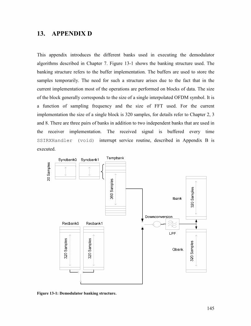
145
13. APPENDIX D
This appendix introduces the different banks used in executing the demodulator
algorithms described in Chapter 7. Figure 13-1 shows the banking structure used. The
banking structure refers to the buffer implementation. The buffers are used to store the
samples temporarily. The need for such a structure arises due to the fact that in the
current implementation most of the operations are performed on blocks of data. The size
of the block generally corresponds to the size of a single interpolated OFDM symbol. It is
a function of sampling frequency and the size of FFT used. For the current
implementation the size of a single block is 320 samples, for details refer to Chapter 2, 3
and 8. There are three pairs of banks in addition to two independent banks that are used in
the receiver implementation. The received signal is buffered every time
SSIRXHandler (void) interrupt service routine, described in Appendix B is
executed.
Figure 13-1: Demodulator banking structure.

146
The samples received at the end of the ISR are buffered in two banks; Syncbank0 and
Syncbank1. Each of these banks is 20 samples wide and is filled alternately. The
doublewindow (void) function calculates the energy of the samples in each of
these banks to obtain the SNR. Once the SNR calculated exceeds the threshold, the
contents of the Syncbank0 and Syncbank1 are transferred to the Tempbank buffer.
This buffer is 360 samples wide and is used to facilitate fine tuning using correlation. The
correlation is calculated over a window of the first 40 samples. After the start of signal is
detected, the 320 samples corresponding to the header are extracted and demodulated.
The outputs of the demodulator are then filtered. The filtered outputs are stored in
Ibank and Qbank, corresponding to the in-phase and quadrature phase components.
The size of Ibank and Qbank is equal to the size of a single OFDM symbol block.
Syncbanks and Tempbank are used exclusively for synchronization and hence are
only used in the initial phase. Once the start of the signal is detected, the received
samples which correspond to the data symbols are stored in Recbank0 and Recbank1
sequentially. The samples are then demodulated, filtered and stored in the Ibank and
Qbank buffer structures. Thus Ibank and Qbank are used over the entire length of
PPDU transmission.
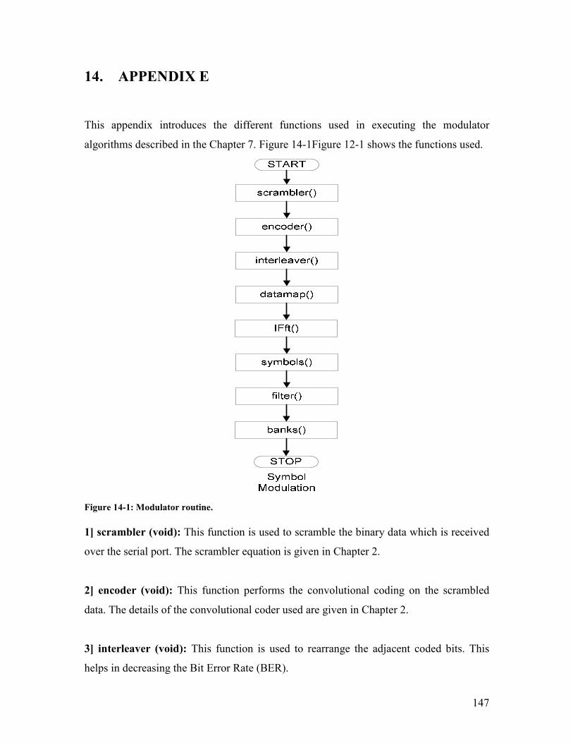
147
14. APPENDIX E
This appendix introduces the different functions used in executing the modulator
algorithms described in the Chapter 7. Figure 14-1Figure 12-1 shows the functions used.
Figure 14-1: Modulator routine.
1] scrambler (void): This function is used to scramble the binary data which is received
over the serial port. The scrambler equation is given in Chapter 2.
2] encoder (void): This function performs the convolutional coding on the scrambled
data. The details of the convolutional coder used are given in Chapter 2.
3] interleaver (void): This function is used to rearrange the adjacent coded bits. This
helps in decreasing the Bit Error Rate (BER).

148
4] datamap (void): This function maps the binary data into the selected QAM
constellation. The mapped symbols are complex with the real part representing the in-
phase component and imaginary part representing the quadrature phase component.
5] Fft (int isgn): This function is used to calculate the Inverse Fast Fourier Transform
(IFFT) to obtain an OFDM symbol. The same function is used in calculating the FFT,
since the both the IFFT and the FFT use the same algorithm. The local argument passed
identifies the operation performed. For the FFT operation the value of local argument
should be 1 while for an IFFT the value of local argument should be -1.
6] symbols (void): This function is used to append the cyclic prefix at the start of the
OFDM data to form an OFDM symbol. For the current implementation the last 16 sample
values of the IFFT output are used to form a cyclic prefix. The purpose of appending a
cyclic prefix is given in Chapter 2.
7] filter (void): This function is used to perform the interpolation operation. The filter
used has 24 coefficients and is implemented in the form of a linear finite impulse
response (FIR) filter. The filter (void) interpolates the in-phase and quadrature
phase components and stores the samples into two buffers: realoutput and
imagoutput which will be described in Appendix F. The filter uses zero-inserting to
upsample the baseband signals. Details of this technique have been given in Chapter 2.
8] banks (void): As described in Chapter 4 the codec is used to communicate the data to
the radio through the ESSI0 interface. This interface is interrupt driven and the Interrupt
Service Routine (ISR) is executed twice every sampling instant. At every sampling
instant, data which is stored in buffer banks is transmitted to the radio. The banks
(void) function is used to perform upconversion and to stack the generated audio band
OFDM signal into the appropriate buffers. The implementation of buffer banks is given
in Appendix F.

149
15. APPENDIX F
This appendix introduces the different banks used in executing the modulator algorithms
described in the Chapter 7. Figure 15-1 shows the banking structure used.
Figure 15-1: Modulator routine.
Analogous to the receiver banking structure, the modulator routine also has a set of
buffers which are used for specific purposes. The modulator routine uses two pairs of
buffers to store the generated OFDM signal. As described in Chapter 4, the OFDM
symbols are interpolated to obtain a baseband representation of the in-phase and
quadrature phase components. The in-phase component is stored in the realoutput
buffer while the quadrature phase component is stored in the imagoutput buffer. Each
of the buffers is 320 samples wide which corresponds to the size of an interpolated
OFDM symbol. These baseband signals are then upconverted by the audio band carrier
150
frequency and added to generate the audio band OFDM signal representation. This signal
is loaded into one of the two banks viz; aa0 and aa1.
As discussed in Appendix A, at every sampling instant, the codec transmits data to the
radio over the left channel and the right channel. In the current implementation only the
right channel is used. In order to keep the implementation of the interrupt service routine
(ISR) simple, the aa banks have audio band OFDM samples stored at alternate
locations. Thus the size of the aa0 and aa1 banks is twice the number of samples per
interpolated OFDM symbol i.e. 640 samples wide. The remaining values are initialized to
zero. This type of arrangement ensures that the codec will always carry data on one of the
two channels.

151
16. APPENDIX G
This appendix introduces the miscellaneous functions which are used in executing the
software algorithms described in Chapter 7. These functions are used in both the routines
or are executed during the modem initialization. The functions are given below.
1] states (void): This function is a part of the initialization routine. In order to expedite
the data modulation, array structures are used which directly map the binary data into
QAM symbols and demap QAM symbols back to binary data. The states (void)
function is used to initialize these array structures.
2] header (void): This function is used to initialize the header coefficients, filter taps and
transmitter banking structure. The header coefficients are used for channel equalization as
described in Chapter 2. In addition, these coefficients are also used to generate the
baseband representation of the PPDU header. The filter coefficients are used to perform
low pass filtering and generate the baseband signals which are stored into respective
buffer banks. The transmitter banking structure was described in detail in Appendix E.
3] ADAInit (void): The codec is used to transfer the OFDM signal to the VHF radio. In
order to initialize the codec the ADAInit (void) function is used. The codec is
programmed to function in network mode and work synchronously based on the internal
clock.
4] DisableReceiveInt (void): This function is used to disable the codec receive interrupt.
The purpose of this function is to ensure that the SSIRXHandler (void) is not
executed at the sampling instances when the modem is functioning in TX mode (transmit
routine). It is called at the beginning of the modulator routine.
5] EnableTransmitInt (void): This function is used in conjunction with the
DisableReceiveInt (void). It enables the codec transmit interrupt.
152
6] EnableReceiveInt (void): It enables the codec receive interrupt. It will be used in the
beginning of receiver routine so that SSIRXHandler (void) will be executed at the
sampling instant.
7] DisableTransmitInt (void): This function is used to disable the codec transmit
interrupt. The purpose of this function is to ensure that the SSITXHandler (void) is
not executed at the sampling instances if the modem is functioning in RX mode. It is
called at the beginning of the receiver routine and is used in conjunction with
EnableReceiveInt (void).
8] WaitForFrameSyncT (void): This function is used to synchronize the interrupts and
the buffer banks in transmitter routine. The codec is programmed to operate in
synchronous mode and both the codec interrupts, receive and transmit, occur at the
sampling instances. At every sampling instant the ISRs are executed twice corresponding
to the right channel and left channel. For the current implementation, the OFDM signal is
transmitted on the right channel. The choice of channel influences the aa banking
structures as discussed in Appendix F. The WaitForFrameSyncT (void)routine
polls the status the Transmit Frame Sync (TFS) bit in the ESSI0 status register. It is
called at the beginning of transmission.
9] WaitForFrameSyncR (void): This function is similar to the WaitForFrameSyncT
(void) and is used in the receiver routine. It polls for the status of the Receive Frame
Sync (RFS) bit in the ESSI0 status register.
153
17. APPENDIX H
This appendix introduces the software flags which are used in executing the software
algorithms described in Chapter 7. These flags functions are used in both the routines and
during the modem initialization.
1] IrqFlag: Asserted when SWITCH A, shown in the circuit diagram in Appendix I is
closed. It is used to exit out of the Main Routine. It gets deasserted when SWITCH B is
closed.
2] overflowflag1: It is used by receiver to realize channel inactivity. The flag is set after
exactly 131.25 msec.
3] overflowflag2: It is used by the receiver to overcome a false alarm. The flag is set
after exactly 656.25 msec.
4] Falsealaramflag: Asserted when overflowflag2 is SET.
5] TXready: This flag is asserted when we receive a response (the number of
packets to be transmitted) for a previously transmitted DTR signal (ASCII character ‘a’).
6] CTSflag: This flag is set when we receive a 'Q' from the NetBurner in response to 'R'.
The handshaking codes associated with these ASCII characters were discussed in
Chapter 5.
7] PreviousMode: This flag is used to signify the previous state/mode for the modem.
8] TXR : This flag is SET when the backoff counter value is reached. This flag is used in
the MAIN routine.
9] FDflag: False detection flag. This is SET when we receive the PTT transience.

154
10] rbflag: Receive buffer flag. This flag is SET when the Receive buffer is full.
11] txflag: Serial Transmit Flag. This flag is SET when the EVM has transmitted 24
bytes of demodulated data to the NetBurner.
12] receivepacket: This counts the number of packets we receive in a single
transmission.
13] symbolcounter: This counts the number of symbols we receive per packet.
14] DebugFlag: Indicates assertion of the IrqFlag.
15] headerflag: This flag is used in the Transmit routine to enforce realignment of stereo
channel used, at the beginning of every packet transmission.
16] packetnumber: This counter counts the number of packets transmitted per
Transmission Slot.
17] serialflag: Serial Receive flag. This flag is SET when the modem receive 24 bytes of
serial data from NetBurner to EVM.
18] isr_count_flag: This flag is used to signify emptying of the aa0/1 banks used in the
modulator. The banking structure was explained in Appendix F.

155
18. APPENDIX I
This appendix discusses the design of the design of daughter card and Interface IV. As
introduced in Chapter 4, Interface IV is used to interface the EVM and radio. There are
three main interfacing lines which need to be connected. They are the microphone input,
PTT line and speaker output.
1] Microphone Input:
This is an input signal for the radio. The codec output on the EVM is connected to the
microphone input. The output from codec is connected to a potentiometer and dc
blocking capacitor. A 10K potentiometer is used to vary the voltage at the input of the
microphone pin. If no voltage divider circuit is used there is a possibility that the codec
output signal will over-modulate the FM carrier.
2] Speaker Output:
This is an output signal for the radio. It is connected to the codec input on the EVM.
Depending upon make of the radio used this signal can be either differential or single
ended. For Motorola XTS 5000, it is differential.
3] PTT Line:
This pin is used to assert and de-assert the push to talk switch. The GPIO pin of Port D is
connected to the PTT line using a relay.
Schematics and the board layout for the daughter card are shown on subsequent pages.

156
19. ACRONYMS
LMR Land Mobile Radio
FM Frequency Modulation
AM Amplitude Modulation
HF High Frequency
VHF Very High Frequency
UHF Ultra High Frequency
TCP Transmission Control Protocol
UDP User Datagram Protocol
IP Internet Protocol
OFDM Orthogonal Frequency Division Multiplexing
DREAMS Disaster Relief and emergency medical services
PHY Physical Layer
MAC Medium Access Layer
OSI Open Systems Interconnection
NBFM Narrowband Frequency Modulation
QAM Quadrature Amplitude modulation
MCM Multi-carrier modulation
DFT Discrete Fourier transform
IDFT Inverse Discrete Fourier transform
FFT Fast Fourier transform
IFFT Inverse Fast Fourier transform
WLAN Wireless Local Area Network
SNR Signal to Noise Ratio
ISI Inter-Symbol Interference
DFE Decision Feedback Equalization
LMS Least Mean Square
EVM Evaluation Module
DSP Digital Signal Processor
BER Bit Error Rate

157
DTE Data Terminal Equipment
DHCP Dynamic Host Configuration Protocol
PTT Push To Talk
CSMA Carrier Sense Multiple Access
CD Collision Detection
CA Collision Avoidance
MPDU MAC Layer Protocol Data Unit
PPDU PHY Layer Protocol Data Unit
DTR Data Terminal Ready
RTS Request To Send
CTS Clear To Send
AWGN Additive White Gaussian Noise
158
20. BIBLIOGRAPHY
1. Milton S. Kiver, “FM Simplified”, 3rd Edition, D. Van Nostrand Company, Inc,
1960.
2. http://www.tapr.org/
3. Pete Lunness, “P25 Radio Systems Training Guide”, TG-001 1-0-1, August 2005.
4. Reinhold Ludwig, Pavel Bretchko, “RF Circuit Design”, Pearson Education,
2000.
5. http://www.dvsinc.com/papers/iambe.htm
6. http://www.motorola.com/content/1,1012,5392,00.html
7. http://www.dreams-project.org/DREAMS/news2.html
8. http://www.faqs.org/rfcs/rfc768.html
9. Herbert Taub, D. Schilling, “Principles of Communication Systems”, 2nd Edition,
Tata McGraw-Hill Publications Ltd., 1971.
10. George Kennedy, Bernard Davis, “Electronic Communication Systems”, 4th
Edition, Tata McGraw-Hill Publications Ltd., 1992.
11. S.B. Weinstein, P.M. Ebert, “Data Transmission by Frequency-Division
Multiplexing using the Discrete Fourier transform”, IEEE Transaction on
Communication Technology, Vol. Com-19,No. 5, OCT 1971.
12. Juha Heiskala, John Terry, OFDM Wireless LANS: A Theoretical and Practical
Guide, SAMS Publication, 2002.
13. http://portal.etsi.org/radio/DigitalAudioBroadcasting/DAB.asp
14. IEEE, “Part 11: Wireless LAN Medium Access Control (MAC) and Physical
Layer (PHY) Specifications”, IEEE Press, 1999,
15. Haiyun Tang, Lau, R. Brodersen, “ Synchronization Schemes for packet OFDM
System” , IEEE International Conference on Communication, Vol 5, May 2003.
16. Timothy Schmidl, D. Cox, “Low-Overhead, Low-Complexity (Burst)
Synchronization for OFDM”, IEEE International Conference on Communications
,Vol 3, June 1996.
17. Jukka Rinne, M. Renfors, "Equalization of Orthogonal Frequency Division
Multiplexing Signals," Global Telecommunications Conference, 1994.
159
GLOBECOM '94. 'Communications: The Global Bridge', IEEE, Pages:415 - 419
vol.1, 28 Nov.-2 Dec. 1994.
18. Ming-Xian Chang, Yu Su, “Performance Analysis of Equalized OFDM Systems
in Rayleigh Fading”, IEEE Transactions on Wireless Communications, Vol 1, No
4, Oct 2002.
19. H. Sari, G. Karam, Jeanclaude, “ Frequency- Domain Equalization of mobile
Radio and Terrestrial Broadcast Channels”, Global Telecommunications
Conference, 1994. GLOBECOM '94. 'Communications: The Global Bridge',
IEEE, vol.1, 28 Nov.-2 Dec. 1994.
20. S. Coleri, M. Ergen, A. Puri, A. Bahai, “A study of channel estimation in OFDM
Systems”, Vehicular Technology Conference, 2002. Proceedings, Volume: 2,
Sept. 2002.
21. K. Pahlavan, A. Levesque, “Wireless Information Network”, 1st Edition, Wiley
Publications, 1995.
22. John Proakis, “Digital Communications”, 4th Edition, McGraw-Hill Publication,
2001.
23. R. Chassaing, “DSP Applications using C and the TMS320C6x DSK”, Wiley
Publications, 2002.
24. G. Clark, “Error correcting coding for digital communications”, Plenum Press,
1981.
25. Tanenbaum, “Computer Networks”, 4th Edition, Prentice-Hall,2002.
26. http://www.faqs.org/rfcs/rfc793.html.
27. W. Stallings, “Data and computer communications”, 7th Edition, Prentice Hall,
2003.
28. Bob O’Harr, Al Petrick, “802.11 Handbook: A designer’s Companion”, IEEE
Press, 1999.
29. http://www.faqs.org/rfcs/rfc2131.html.
30. Gaith Hammouri , “Obits Modem: Netburner Daughter Card Interface”, WPI,
2005.
31. T. Rappaport, “ Wireless Communications”, Prentice Hall, 1996.

160
32. John Proakis, D. Manolakis, “Digital Signal Processing”, 3rd Edition, Prentice
Hall, 2002.
33. Simon Haykin, “Adaptive Filter Theory”, 3rd Edition, Prentice Hall, 1996.