design of a 'figure-8' spherical motion flapping wing for
TRANSCRIPT
UNLV Theses, Dissertations, Professional Papers, and Capstones
5-2009
Design of a "Figure-8" Spherical Motion Flapping Wing for Design of a "Figure-8" Spherical Motion Flapping Wing for
Miniature UAV's Miniature UAV's
Zohaib Parvaiz Rehmat University of Nevada, Las Vegas
Follow this and additional works at: https://digitalscholarship.unlv.edu/thesesdissertations
Part of the Aeronautical Vehicles Commons, Mechanical Engineering Commons, Navigation,
Guidance, Control and Dynamics Commons, and the Structures and Materials Commons
Repository Citation Repository Citation Rehmat, Zohaib Parvaiz, "Design of a "Figure-8" Spherical Motion Flapping Wing for Miniature UAV's" (2009). UNLV Theses, Dissertations, Professional Papers, and Capstones. 1204. http://dx.doi.org/10.34917/2754424
This Thesis is protected by copyright and/or related rights. It has been brought to you by Digital Scholarship@UNLV with permission from the rights-holder(s). You are free to use this Thesis in any way that is permitted by the copyright and related rights legislation that applies to your use. For other uses you need to obtain permission from the rights-holder(s) directly, unless additional rights are indicated by a Creative Commons license in the record and/or on the work itself. This Thesis has been accepted for inclusion in UNLV Theses, Dissertations, Professional Papers, and Capstones by an authorized administrator of Digital Scholarship@UNLV. For more information, please contact [email protected].

DESIGN OF A "FIGURE - 8" SPHERICAL MOTION FLAPPING
WING FOR MINIATURE UAV'S
by
Zohaib Parvaiz Rehmat
Bachelor of Science Vaughn College of Aeronautics and Technology, New York, USA
2005
A thesis submitted in partial fulfillment of the requirements for the
Master of Science Degree in Mechanical Engineering Department of Mechanical Engineering
Howard R. Hughes College of Engineering
Graduate College University of Nevada, Las Vegas
May 2009

UMI Number: 1472437
INFORMATION TO USERS
The quality of this reproduction is dependent upon the quality of the copy
submitted. Broken or indistinct print, colored or poor quality illustrations
and photographs, print bleed-through, substandard margins, and improper
alignment can adversely affect reproduction.
In the unlikely event that the author did not send a complete manuscript
and there are missing pages, these will be noted. Also, if unauthorized
copyright material had to be removed, a note will indicate the deletion.
®
UMI UMI Microform 1472437
Copyright 2009 by ProQuest LLC All rights reserved. This microform edition is protected against
unauthorized copying under Title 17, United States Code.
ProQuest LLC 789 East Eisenhower Parkway
P.O. Box 1346 Ann Arbor, Ml 48106-1346

Copyright by Zohaib Parvaiz Rehmat 2009 All Rights Reserved

Thesis Approval The Graduate College University of Nevada, Las Vegas
Apri 1 78 ,20Q3_
The Thesis prepared by
Zohaib Parva iz Rehmat
Entitled
Design of a "Figure-8" Spherical Motion Flapping Wing for Miniature
imv's
is approved in partial fulfillment of the requirements for the degree of
Master of Science i n Mechanical Engineer ing
Examination Committee Kjo-Qwir
Examination Committee Member
E/aminatnoJn Committee Member
Graduate College Faculty Representative
Examination Committee Chair
Dean of the Graduate College
1017-53 11

ABSTRACT
Design of a "Figure - 8" Spherical Motion Flapping Wing for Miniature UAV's
by
Zohaib Parvaiz Rehmat
Dr. Mohamed B. Trabia, Examination Committee Co-Chair/Professor Dr. Woosoon Yim, Examination Committee Co-Chair/Professor
Department of Mechanical Engineering University of Nevada, Las Vegas
Hummingbirds and some insects exhibit a Figure-8 motion, which allows them to
undergo variety of maneuvers including hovering. It is therefore desirable to have
flapping wing miniature air vehicles (FWMAV) that can replicate this unique wing
motion. In this research, a design of a flapping wing for FWMAV that can mimic Figure -
8 motion using a spherical four bar mechanism is presented. To produce Figure-8 motion,
the wing is attached to the coupler point of the spherical four bar mechanism and driven
by a DC servo motor. For verification of the design, a prototype of the wing and
mechanism is fabricated to determine whether the design objectives are met.
Additionally, experimental testing is conducted to determine the feasibility of this design
with the wing driven at speeds ranging from 2.5 to 12.25 Hz. To determine the
aerodynamic coefficients the wing experiences during the Figure-8 cycle, wind tunnel
experimentation is conducted. The results show good correlation between the model and
experimental testing.
iii
TABLE OF CONTENTS
ABSTRACT iii
TABLE OF CONTENTS iv
LIST OF FIGURES vii
LIST OF TABLES xi
ACKNOWLEDGEMENTS xii
CHAPTER 1 INTRODUCTION 1
CHAPTER 2 LITERATURE REVIEW 4 2.1 Overview 4 2.2 Biological Flight Classification 4 2.3 Bio-Inspired Flapping Wing Mechanical Concepts 9 2.4 Flapping Wing Design Validation 13
2.4.1 Experimental Investigation Approach 14 2.5 Spherical Motion Approach 18
2.5.1 Spherical Four-Bar Mechanism for Flapping Wing Design 18 2.5.2 Spherical Four-Bar Mechanism Synthesis Review 18
CHAPTER 3 SPHERICAL FOUR-BAR MECHANISM 20 3.1 Create Bio-Inspired Mechanism 20 3.2 Mechanism Concept 21
3.3.1 Figure-8 Symmetry Conditions 23 3.3.2 Motion Synthesis of Figure-8 Phases 25
3.4 Resulting Figure-8 Spherical Motion 29
CHAPTER 4 MECHANICAL DESIGN PROCESS 32 4.1 Objective..... 32 4.2 Design Requirements 32
4.2.1 Size Requirement 33 4.2.2 Weight Requirement 33 4.2.3 Flapping Frequency Requirement 34
4.3 Spherical Four-Bar Mechanism Design 34 4.3.1 Design 34 4.3.1 Fabrication 37
4.4. Wing 39 4.4.1 Design 39
iv

4.4.2 Fabrication 40 4.5 Prototype 41
CHAPTER 5 PROTOTYPE TESTING 44 5.1 Objective 44 5.2 Prototype Test Stand/Platform 44 5.3 Apparatus/Hardware 45
5.3.1 Six-Axis F/T Load Cell 46 5.3.2 Motor Selection 48
5.4 Testing 49 5.4.1 Motor Control Optimization 49 5.4.2 Pre-Testing Conditions 55
5.5 Data Analysis 56 5.5.1 Filtering 56
5.6 Force Signal Interpretation 57 5.6.1 Chord-wise Force, Fx, Interpretation 57 5.6.2 Normal Force, Fy, Interpretation 59
5.6 Motion Verification 60
CHAPTER 6 WIND TUNNEL TESTING 63 6.1 Objective 63 6.2 Free Stream Velocity and Angle of Attack 64 6.3 Setup and Apparatus 66
6.3.1 Setup Conditions 69 6.3.2 Motor Control in Stepper Mode 69
6.4 Quasi-Static Analysis 70 6.4.1 Coefficients of Axial and Normal Force 70 6.4.2 Coefficients of Lift and Drag 73
6.4.3 Center of Pressure 76 6.5 Dynamic Analysis 78
6.5.1 Coefficients of Axial and Normal Force 79 6.5.2 Coefficients of Lift and Drag 82 6.5.3 Center of Pressure 83
CHAPTER 7 PROTOTYPE TESTING RESULTS 87 7.1 Force Signal Analysis 87 7.2 Signal Filtering at 12.25 Hz 87 7.3 Force Plots at 12.25 Hz 89
7.3.1 Chord-wise Force, Fx, at 12.25 Hz 89 7.3.2 Normal Force, Fy, at 12.25 Hz 91 7.3.3 Span-wise Force, Fz, and the other Force Components 92
CHAPTER 8 CONCLUSIONS 98 8.1 Spherical Four-Bar Mechanism Assessment 98 8.2 Design and Motion Verification 99 8.3 Potential Flight Characteristics of Figure-8 Motion 101 8.4 Prototype Testing Evaluation 101
v

8.5 Future Work 102
REFERENCES 104
APPENDIX A EQUATIONS OF MOTION FOR FIGURE-8 SPHERICAL MOTION 107
APPENDIX B HIGH SPEED CAMERA TESTING 108
APPENDIX C AERODYNAMIC MODELING 113 C.l Defining Induced Free-stream Velocity 113 C.2 Projection of the Free-stream Velocity onto the Wing,(Vn & Va) 114 C.3 Derivation of Aerodynamic Forces 117 C.4 Attached Flow 118 C.5 Detached (Stalled) Flow 119 C.6 Dynamic Stall Condition 121
APPENDIX D CFD MODELING 122
APPENDIX E PROTOTYPE TESTING PLOTS 123
VITA 147
VI

LIST OF FIGURES
Figure 2.1 Horizontal Stroke Plane Wing Motion as seen in Hummingbirds, [1] 6 Figure 2.2 Inclined Stroke Plane Motion, i.e. Bats and Dragonflies, [1] 6 Figure 2.3 Vertical Stroke Plane Motion, Butterflies, [1] 7 Figure 2.4 Lift Generation of a hummingbird while in hover is seen in up-stroke and
down-strokes during both the forward and backward strokes of the flapping motion, [2] 8
Figure 2.5 Planar Four-Bar Mechanism Used to Generate Figure-8 Motion, [4] 10 Figure 2.6 Prototype of FWMAV with double Scotch Yoke Spherical Mechanism
Which Produces Figure-8 Motion, [6] 10 Figure 2.7 Prototype of FWMAV with Out-of-Stroke Plane Motion, [7] 11 Figure 2.8 FWMAV Prototype with Mechanism Capable of Biaxial Rotation, [8] 12 Figure 2.9 Parallel Crank-Rocker Flapping Mechanism, [10] and [11] 13 Figure 2.10 (A) Robotic Fly Immersed in 1 m x lm x 2m tank of mineral oil, and (B)
close up view of robotic flapper, [13] 15 Figure 2.11 Robotic Flapper used for experimentation in [17] and [18] 17 Figure 3.1 Spherical Four-Bar Mechanism 22 Figure 3.2 Wing Point Trajectory and Induced Velocity 23 Figure 3.3 Spherical Four-Bar Mechanism, 04 is equal to 0° 25 Figure 3.4 Spherical Four-Bar Mechanism, 84 is equal to 90° 26 Figure 3.5 Spherical Four-Bar Mechanism, 64 is equal to 180° 27 Figure 3.6 Spherical Four-Bar Mechanism, 84 is equal to 270° 28 Figure 3.7 Motion of the Spherical Four-Bar Mechanism 30 Figure 3.8 Wing Trajectory with Center of Gravity 31 Figure 4.1 Location of Each Mechanism Link amongst the Greater Sphere 36 Figure 4.2 Proposed Conceptual Design of Spherical Four-Bar Mechanism 37 Figure 4.3 Machined Links Used to Construct Spherical Four-Bar Mechanism 38 Figure 4.4 (A) Dragonfly forewing used in [16] . (B) Proposed Wing Design for
Prototype and Testing 39 Figure 4.5 Wing Top View 40 Figure 4.6 Conceptual and Actual Prototype of Spherical Four-Bar Mechanism 42 Figure 4.7 Wing Design for the FWMAV Prototype 43 Figure 4.8 Figure-8 Spherical Four Bar Mechanism 43 Figure 4.9 Prototype of the Figure-8 Spherical Four Bar Mechanism 43 Figure 5.1 Wing Prototype Test Stand 45 Figure 5.2 ATI-IA Nano 17 F/T Sensor LabVIEW Virtual Instrumentation 48 Figure 5.3 For 2.5 Hz Flapping, (A) Speed Output at 150 RPM with Tuned Controller
Gains and (B) Motor Power Consumption for This Speed 51 Figure 5.4 For 5 Hz Flapping, (A) Speed Output at 300 RPM with Tuned Controller
Gains and (B) Motor Power Consumption for This Speed 52
vii
Figure 5.5 For 7.5 Hz Flapping, (A) Speed Output at 450 RPM with Tuned Controller Gains (B) Motor Power Consumption for This Speed 53
Figure 5.6 For 10 Hz Flapping, (A) Speed Output at 600 RPM with Tuned Controller Gains and (B) Motor Power Consumption for This Speed 54
Figure 5.7 For 12.25 Hz Flapping, (A) Speed Output at 735 RPM with Tuned Controller Gains and (B) Motor Power Consumption for This Speed 55
Figure 5.8 Wing Prototype at the Initial Position of Figure-8 with Load Cell Attached and Coordinate Frame Assigned 56
Figure 5.9 Chord-wise Force, Fx, Representation for Figure-8 Cycle 58 Figure 5.10 Normal Force, Fy, Representation for Figure-8 Cycle 59 Figure 5.11 Figure-8 Motion Trajectory Generated at 10 Hz 61 Figure 5.12 Figure-8 of High Speed Motion Capture of Point 22 of Figure A.2 62 Figure 6.1 Wing Point Trajectory and Induced Velocity 64 Figure 6.2 Free Stream Velocity, V, and Velocity along the Wing Edge, U 64 Figure 6.3 Variation in Angle of Attack in the Figure-8 Cycle 65 Figure 6.4 Cross-sectional View of Airfoil with Cp and Aerodynamic Forces 66 Figure 6.5 Conceptual Rendering of Wind Tunnel Experimentation 67 Figure 6.6 Wind Tunnel Experimentation Setup 68 Figure 6.7 Wing Rotation in Wind Tunnel With Respect to Angle of Attack 68 Figure 6.8 Force Signal, Fx, for Quasi-Static Wind Tunnel Testing 72 Figure 6.9 Force Signal, Fy, for Quasi-Static Wind Tunnel Testing 72 Figure 6.10 Coefficient of Axial Force, Ca, from 0-90° Angle of Attack for Quasi-Static
Wind Tunnel Simulation 73 Figure 6.11 Coefficient of Normal Force, C„, from 0-90° Angle of Attack for Quasi-
Static Wind Tunnel Simulation 73 Figure 6.12 Coefficient of Lift, Q, and Drag, d, for 0-90° Angle of Attack for Quasi-
Static Wind Tunnel Simulation 74 Figure 6.13 Cp Position Vector, R, Definition 76 Figure 6.14 Change in Center of Pressure, Cp, in Chord-wise and Span-wise Direction
for 0-90° Angle of Attack 78 Figure 6.15 Force Signal, Fx, for Dynamic Wind Tunnel Testing 80 Figure 6.16 Force Signal, Fy, for Dynamic Wind Tunnel Testing 80 Figure 6.17 Coefficient of Axial Force, Ca, from 0-90° Angle of Attack for Dynamic
Wind Tunnel Simulation 81 Figure 6.18 Coefficient of Normal Force, C„, from 0-90° Angle of Attack Dynamic
Wind Tunnel Simulation 81 Figure 6.19 Coefficient of Lift, C,, and Drag, Cd, for 0-90° Angle of Attack 82 Figure 6.20 Change in Center of Pressure, Cp, in Chord-wise and Span-wise Direction
for 0-90° Angle of Attack, Dynamic Testing 84 Figure 6.21 Discontinuity in Cpfor Dynamic Change in Angle of Attack 84 Figure 6.22 Coefficient of Drag, Q , Determined by CFD Modeling, Appendix D, and
Wind Tunnel Testing 85 Figure 6.23 Coefficient of Lift, C;, Determined by CFD Modeling, Appendix D, and
Wind Tunnel Testing 86 Figure 7.1 Unfiltered and Filtered Force Signal for Chord-wise Force, Fx, at 12.25 Hz
88
viii
Figure 7.2 Unfiltered and Filtered Force Signal for Normal Foree, Fy, at 12.25 Hz 89 Figure 7.3 Chord-wise Force, Fx, at 12.25 Hz 90 Figure 7.4 Normal Force, Fy, at 12.25 Hz 91 Figure 7.5 Span-wise Force, Fz, at 12.25 Hz 94 Figure 7.6 Force Magnitude of Chord-wise, Fx, and Normal Force, Fy, at 12.25 Hz.... 94 Figure 7.7 Force Magnitude, F, at 12.25 Hz 95 Figure 7.8 Moment, Mx, at 12.25 Hz 95 Figure 7.9 Moment, My, at 12.25 Hz 96 Figure 7.10 Moment, Mz, at 12.25 Hz 96 Figure 7.11 Moment Magnitude, M, at 12.25 Hz 97 Figure C.l Wing Point Trajectory & induced velocity 114 Figure C.2 Induced wing velocity projection 115 Figure C.3 Approximate Wing-Sub Area Divisions 116 Figure C.4 Wing Section Aerodynamics forces and motion variables 118 Figure E.l Unfiltered Data FFT for Chord-wise Force, Fx, at 12.25 Hz 124 Figure E.2 Unfiltered Data FFT for Normal Force, Fy, at 12.25 Hz 124 Figure E.3 Unfiltered Data FFT for Chord-wise Force, Fx, at 2.5 Hz 125 Figure E.4 Unfiltered Data FFT for Normal Force, Fy, at 2.5 Hz 126 Figure E.5 Chord-wise Force, Fx, at 2.5 Hz 127 Figure E.6 Normal Force, Fy, at 2.5 Hz 127 Figure E.7 Span-wise Force, Fz, at 2.5 Hz 128 Figure E.8 Force Magnitude of Chord-wise, Fx, and Normal Force, Fy, at 2.5 Hz 128 Figure E.9 Force Magnitude, F, at 2.5 Hz 129 Figure E.10 Moment, Mx, at 2.5 Hz 129 Figure E.l 1 Moment, My, at 2.5 Hz... 130 Figure E.12 Moment, Mz, at 2.5 Hz 130 Figure E.13 Moment Magnitude, M, at 2.5 Hz 131 Figure E.14 Chord-wise Force, Fx, at 5 Hz 132 Figure E.15 Normal Force, Fy, at 5 Hz 132 Figure E.16 Span-wise Force, Fz, at 5 Hz 133 Figure E.l7 Force Magnitude of Chord-wise, Fx, and Normal Force, Fy, at 5 Hz 133 Figure E.18 Force Magnitude, F, at 5 Hz 134 Figure E.19 Moment, Mx, at 5 Hz 134 Figure E.20 Moment, My, at 5 Hz 135 Figure E.21 Moment, Mz, at 5 Hz 135 Figure E.22 Moment Magnitude, M, at 5 Hz 136 Figure E.23 Chord-wise Force, Fx, at 7.5 Hz 137 Figure E.24 Normal Force, Fy, at 7.5 Hz 137 Figure E.25 Span-wise Force, Fz, at 7.5 Hz 138 Figure E.26 Force Magnitude of Chord-wise, Fx, and Normal Force, Fy, at 7.5 Hz 138 Figure E.27 Force Magnitude, F, at 7.5 Hz 139 Figure E.28 Moment, Mx, at 7.5 Hz 139 Figure E.29 Moment, My, at 7.5 Hz 140 Figure E.30 Moment, Mz, at 7.5 Hz 140 Figure E.31 Moment Magnitude, M, at 7.5 Hz 141 Figure E.32 Chord-wise Force, Fx, at 10 Hz 142
IX

Figure E.33 Normal Force, Fy, at 10 Hz 142 Figure E.34 Span-wise Force, Fz, at 10 Hz 143 Figure E.35 Force Magnitude of Chord-wise, Fx, and Normal Force, Fy, at 10 Hz 143 Figure E.36 Force Magnitude, F, at 10 Hz 144 Figure E.37 Moment, Mx, at 10 Hz 144 Figure E.38 Moment, My, at 10 Hz 145 Figure E.39 Moment, Mz, at 10 Hz 145 Figure E.40 Moment Magnitude, M, at 10 Hz 146
x

LIST OF TABLES
Table 3.1 Variables of Spherical Four-Bar Mechanism 22 Table 3.2 Spherical Four-Bar Mechanism Link Angular Dimensions 24 Table 4.1 Mechanism Links Concentric Spherical Radii 36 Table 4.2 Mass of Links and Assembly Components for Mechanism 38 Table 5.1 ATI-IA Nano 17 Load Cell Calibrations 47 Table 5.2 PI Controller Gains at Different Wing Flapping Frequency 50 Table 6.1 Motor Testing Parameters for Quasi-Static Testing 70 Table 6.2 Testing Conditions and Parameters for Quasi-Static Testing 71 Table 6.3 Motor Testing Parameters for Dynamic Testing 79 Table 6.4 Testing Conditions and Parameters for Dynamic Testing 79 Table B.l Specifications of High Speed Camera 108 Table B.2 Stereo Camera Intrinsic Parameters 111 Table B.3 Stereo Camera Extrinsic Parameters I l l
XI
ACKNOWLEDGEMENTS
I would like to thank my advisors, Dr. Mohamed Trabia and Dr. Woosoon Yim, for
their encouragement, assistance, and guidance throughout my graduate studies at UNLV.
I would like thank members of advisory committee for their suggestions and
comments.
I would like to thank fellow friend and research partner Jesse A. Roll for his
dedication and commitment to this project. It was a pleasure working with him and I wish
him the best on his future endeavors.
Lastly, I would like to thank my parents for their encouragement and guidance. I
would not be here without them.
xii
CHAPTER 1
INTRODUCTION
Unmanned Aerial Vehicle (UAV) design has shown an evolutionary trend during the
past quarter century stemming from the desire to reproduce what is seen in nature. The
exploration in UAV design began with the concept of recreating fixed wing flight at a
smaller scale since it was well understood. The concept of inducing flight by creating
thrust using a propeller or other mean and generating lift by the pressure difference
created by the free stream velocity provided a simplistic and practical UAV design.
Commonly used fixed wing UAV's provided a usable design for many military,
reconnaissance, and civilian applications. However, fixed wing UAV's provided no
design challenges and little enhancements to be made since maneuverability is limited at
most. The flight mechanics seen in nature, birds and insects, has proposed another
technique that can be utilized to enhance UAV design. Nature's flying animals use their
flapping wings to generate thrust and create lift with superior maneuverability and
mobility throughout flight.
Flapping wings flight can yield many benefits to UAV design. Recent advances in the
study of the biological understanding of bird and insect flapping wings has motivated
many researchers to recreate these many flapping motions in a mechanized form. In
essence, the versatility exhibited during flight by birds and insects has created a design
model for UAV design. The various distinctive flapping patterns provide researchers
1

many design options in accordance with the flight characteristics desired. Nevertheless,
flapping wing unmanned air vehicles (FWMAV) can provide greater usage as they can
travel about confined areas, hover, and easily modulate direction. These ideal
characteristics have made many researchers dedicated in the design and modeling of
FWMAVs.
The potential of FWMAVs seem promising; however, mimicking nature involves
great difficulty and engineering challenges. Nature's unique flight patterns are complex
and at a small scale. To replicate these flapping patterns, a thorough understanding of the
motion pattern is required to design a precise mechanism. The wings must be carefully
designed and fabricated to retain many of the characteristics present in bird and insect
wings, i.e. light and flexible. The modeling of unsteady aerodynamic is another aspect
that needs careful attention. Bird and insect flight is at low Reynolds number regime, thus
overall aerodynamic forces may be very small. With all these considerations, FWMAV
design requires extensive engineering and biological understanding for successful
application.
In this research, we will present a bio-inspired wing mechanism design based on the
flight pattern of hovering birds and insects, primarily the hummingbird. Hummingbirds
and some insects outline a Figure-8 spherical motion trajectory enabling high
maneuverability and hovering capabilities. Considering these characteristics, this wing
motion provides desirable option for integration with FWMAVs. To produce Figure-8
spherical motion, a spherical four-bar mechanism was designed such that a wing attached
to coupler point would outline the desire motion. Following the design and fabrication
process, a setup is devised to conduct experimentation that would elucidate whether the
2

wing trajectory is achieved. A force signal will be measured with the wing in motion at
increasing frequencies. The measured force signal will be used to predict the forces
induced by this motion and serve as validation for the modeling of this motion.
Additionally, an experimental approach using a subsonic wind tunnel is setup to
determine the lift and drag associated with this flapping motion. This purpose of research
was to determine a reasonable design for a Figure-8 spherical motion flapping using a
unique design and conduct experimentation, determine the force model of the associated
forces produces, and create a CFD model. This thesis will discuss the subtask of design
and experimentation of a Figure-8 spherical motion flapping wing.
3

CHAPTER 2
LITERATURE REVIEW
2.1 Overview
Flapping Wing Miniature Air Vehicles (FWMAV) can offer potential abilities that
stand unmatched compared to fixed wing flight. Nature's flying animals' exhibit mobility
and maneuverability to travel about confined spaces, hover, and modulate direction with
minimal effort and without loss of balance. These ideal behavioral aspects are desirable
in the expansion of UAV design with the implementation of flapping wings that can
recreate the motion seen in nature. Considering the exceptional benefits integration of
flapping wings can offer to UAV design, researchers have tried to understand and
quantify the flight aspects as exhibited in nature to begin the exploration of flapping wing
UAVs. Researchers have also dedicated their time in producing a design that can
replicate flapping patterns as seen in nature. In doing so, the biological foundation
allowing bird and insect flapping wing flight must also be well understood.
2.2 Biological Flight Classification
Comprehension of flight seen in nature is needed in order to employ the same
concepts in flapping wing designs. Flapping wings typically exhibit complex motion that
simultaneously combines three angles: heaving (back and forth motion in the stroke
plane), stroke (angle out of the stroke plane), and feathering (twist around the wing axis).
4

Many researchers studied various aspects of flapping wing motion of insects and birds.
The following is a brief survey of the work presented which identifies certain aspects of
flapping motion.
Ellington, [1], researched the flapping motion dynamics seen in nature. His work
signifies that flapping motions can yield high lift and thrust values within low Reynolds
number flight regimes. The minimal effect of inertial force contribution in this case
maximizes the aerodynamics of flapping wing flight that provides the ability for various
maneuvers as compared to fixed wing flight. Kinematic groups that pertain to the
flapping patterns most commonly seen in nature are also outlined in this study. These
patterns can be generally classified according to stroke planes. Stroke planes are
conventionally defined as the plane to which wing stroke is confined. The three types of
stroke planes identified are Horizontal Stroke Planes (hummingbirds and most insects),
Inclined Stroke Planes (bats, passerine birds, and dragonflies), and Vertical Stroke Planes
(butterflies). The flight uniqueness of each stroke plane is detailed in his work. Examples
of the flapping patterns categorized by stroke planes can be seen in Figures 2.1 to 2.3.
5

Figure 2.1 Horizontal Stroke Plane Wing Motion as seen in Hummingbirds, [1]
^
M in
Figure 2.2 Inclined Stroke Plane Motion, i.e. Bats and Dragonflies, [1]
6

Figure 2.3 Vertical Stroke Plane Motion, Butterflies, [1]
The research by Shyy et al. [2] details the factors that affect scaling laws of biological
and micro air vehicles such as wing span, wing loading, vehicle mass, cruising speed,
flapping frequency, and power. Kinematics of flapping wings and an aerodynamic model
for lift and drag forces associated with flapping motions are also presented. The research
also enlightens on the ability of a hummingbirds to produce lift during both the up-stroke
and down-stroke phases of its motion enabling it to hover. Figure 2.4 shows a
hummingbird cycling through its flapping motion as it hovers.
7

Figure 2.4 Lift Generation of a hummingbird while in hover is seen in up-stroke and
down-strokes during both the forward and backward strokes of the flapping motion, [2]
For micro air vehicle design consideration, Ellington [3] presents insight on the
ability of insects to produce high lift ratios by different techniques during the flapping
motion cycle. The effects of wing frequencies and power demands as a function of the
mass of the vehicle are presented. The paper concludes by outlining design challenges
consisting of the mass, power, and maximum speed of insect-based micro air vehicles
that would need to be resolved for successful autonomous designs. These design
challenges will limit applicable FWMAV designs since the probability of achieving a
balance of all three aspects is difficult. In nature, birds and insects have limited mass,
require little power for flapping, and reach beat frequencies of up to 200 Hz, i.e.
hummingbirds. Nonetheless, researchers seem undeterred as many design concepts are
presented in hopes of creating succesful FWMAVs.
8
2.3 Bio-Inspired Flapping Wing Mechanical Concepts
The research available on the flight patterns of birds and insects has paved the way
for research in the development of flapping wing miniature air vehicles with different
mechanical concepts that attempt to reproduce what is seen in nature. The fascination of
researchers with creating FWMAVs has yielded unique designs that accomplish various
flapping wing motions. A summary of the mechanical design concepts introduced by
many researchers are discussed.
To generate insect-like flapping motion, a planar four-bar mechanism is utilized by
Zbikowski et al. [4]. The four-bar mechanism is designed to outline figure-of-eight wing
path similar to many hovering insects. Figure 2.5 displays the configuration of the four
bar mechanism used to generate the desired wing motion. A wing using a composite
frame and Mylar membrane is a feasible option explored in the research. Using the
mechanism concept and wing design, a prototype is fabricated to determine the forces
induced at a wing beat frequency of up to 20 Hz and compared to those produced by
unsteady aerodynamics. Similarly, Zbikowski et al. [5] presents the insect-like flapping
kinematics of hover with a four-bar linkage and a spatial articulation. By re-configuring
the coupler link, planar figure-of-eight motion is transformed into spherical Figure-8
motion at the wing tips. This design enhancement provided a more practical design since
it creates more precise wing motion. Furthermore, Galinski and Zbikowski, [6], expand
on their ongoing research by incorporating a spatial mechanism to improve their design.
A spherical double Scotch yoke is integrating into the design to produce Figure-8 wing
motion as a spherical Lissajous' curve. This design enhancement provides a smoother
9

spherical curve as compared to Figure-8 motion generated by the planar mechanism. The
complete mechanism with the addition of the double Scotch yoke is shown in Figure 2.6.
Figure 2.5 Planar Four-Bar Mechanism Used to Generate Figure-8 Motion, [4]
^2? A*
Figure 2.6 Prototype of FWMAV with double Scotch Yoke Spherical Mechanism
Which Produces Figure-8 Motion, [6]
Banala and Agrawal, [7], designed a single degree of freedom multipart mechanism
consisting of a five bar mechanism and an auxiliary four bar mechanism. The mechanism
10
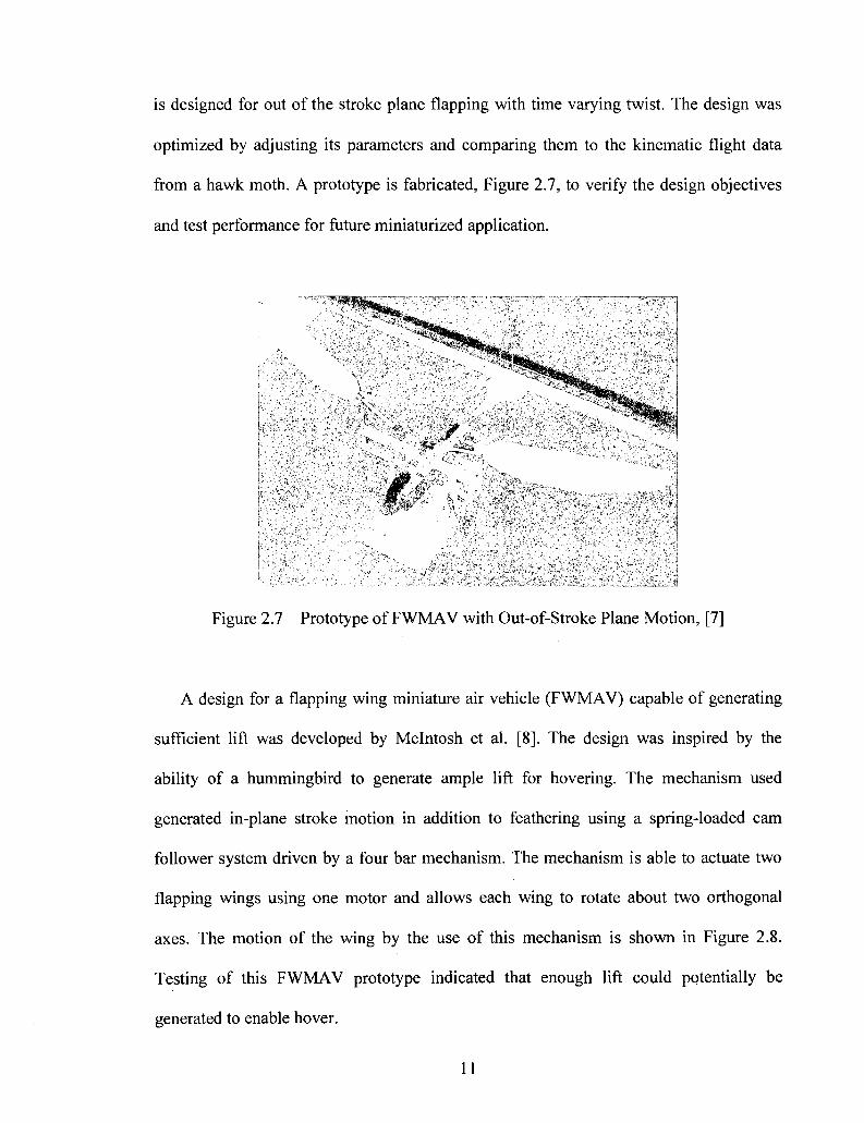
is designed for out of the stroke plane flapping with time varying twist. The design was
optimized by adjusting its parameters and comparing them to the kinematic flight data
from a hawk moth. A prototype is fabricated, Figure 2.7, to verify the design objectives
and test performance for future miniaturized application.
Figure 2.7 Prototype of FWMAV with Out-of-Stroke Plane Motion, [7]
A design for a flapping wing miniature air vehicle (FWMAV) capable of generating
sufficient lift was developed by Mcintosh et al. [8]. The design was inspired by the
ability of a hummingbird to generate ample lift for hovering. The mechanism used
generated in-plane stroke motion in addition to feathering using a spring-loaded cam
follower system driven by a four bar mechanism. The mechanism is able to actuate two
flapping wings using one motor and allows each wing to rotate about two orthogonal
axes. The motion of the wing by the use of this mechanism is shown in Figure 2.8.
Testing of this FWMAV prototype indicated that enough lift could potentially be
generated to enable hover.
11

Figure 2.8 FWMAV Prototype with Mechanism Capable of Biaxial Rotation, [8]
Optimization of the flapping process was explored by Mandangopal et al. [9] by
designing an energy storage mechanism that can be integrated into FWMAV designs.
This design is based on the function of the insect thorax to store elastic potential energy
for release in the subsequent stroke. The concept presented provides a technique to limit
peak torque requirements of the drive motor of FWMAV prototypes.
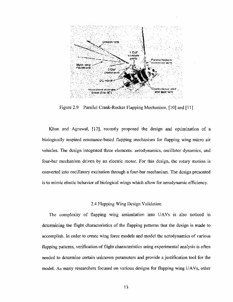
Other ongoing research continues to present design ideas for FWMAV application. A
novel micro air vehicle design with the objective of reproducing the unsteady
aerodynamics of insect flight is presented by Conn et al., [10] and [11], using a parallel
crank rocker mechanism. This mechanism discussed, PCR, allows for unconstrained
motion as compared to other designs because of an integrated flapping and pitching
motion output. The mechanism is designed such that a phase lag between two linkages
can alter the wing angle of attack. By controlling the wing angle of attack, this
mechanism allows for control of pitching facilitating greater maneuverability induced by
adjusting the wing angle of attack and beat frequency as compared to other FWMAV
wing mechanisms. Figure 2.9 shows the parallel crank rocker mechanism presented by
the authors.
1 %
/v.i*«w>=-.ws' fNnw«viMtMj»
12
raveSute r
p w»* if. te Sf s . a « s»w ««*
Figure 2.9 Parallel Crank-Rocker Flapping Mechanism, [10] and [11]
Khan and Agrawal, [12], recently proposed the design and optimization of a
biologically inspired resonance-based flapping mechanism for flapping wing micro air
vehicles. The design integrated three elements: aerodynamics, oscillator dynamics, and
four-bar mechanism driven by an electric motor. For this design, the rotary motion is
converted into oscillatory excitation through a four-bar mechanism. The design presented
is to mimic elastic behavior of biological wings which allow for aerodynamic efficiency.
2.4 Flapping Wing Design Validation
The complexity of flapping wing assimilation into UAVs is also noticed in
determining the flight characteristics of the flapping patterns that the design is made to
accomplish. In order to create wing force models and model the aerodynamics of various
flapping patterns, verification of flight characteristics using experimental analysis is often
needed to determine certain unknown parameters and provide a justification tool for the
model. As many researchers focused on various designs for flapping wing UAVs, other
13

researchers have primarily focused on experimental investigation and modeling of
flapping wing UAVs to substantiate their abilities. An outline of experimental techniques
used by researchers is detailed in this section.
2.4.1 Experimental Investigation Approach
Extensive experimental testing is conducted by researchers as a means of determining
factors that can yield a FWMAV capable of mimicking a bird or insect. To comprehend
how enough force is produced by insects, Dickenson et al., [13], did testing with a
dynamically scaled wing model of a fruit fly, termed robotic fly. To simulate airflow
around the wing, it is immersed in mineral oil with a load cell attached to the base and
driven by a set of stepper motors for flapping in accordance with the actual flight pattern
of a fruit fly, Figure 2.10. With this study, the authors presented the concept that flapping
motion of insects is a function of three distinct and interactive mechanisms that generate
lift at low Reynolds number flight. The translational stroke enables delayed stall by
sweeping the air at large angles of attack and the production of aerodynamic forces occur
during rotational circulation and wake capture as stroke reversing by quickly rotating and
changing direction. The author also elaborates on the high maneuverability and hovering
made possible by the two rotational mechanisms.
14

motor assembly
idS coaxial
drive shaft
force sensor
mineral oil
model wrtg
force vector
wing i chord 1 -
force sensor
i r iN gearbox
A- model wing
Figure 2.10 (A) Robotic Fly Immersed in 1 m x lm x 2m tank of mineral oil, and (B)
close up view of robotic flapper, [13]
The aerodynamics force generated by wing rotation is examined Sane and Dickenson,
[14]. An aerodynamic force signal is obtained by a steady translating wing which is
rotated at constant angular velocities with results then incorporated into traditional,
translational based models of insect flight. This study attempted to determine the
aerodynamics force contribution associated simply with wing rotation. Incorporating the
rotational effects into flapping wing models provides more precise modeling in turn
assisting researchers in predicting the generated forces of flapping wings.
Considering the low Reynolds number flight regime and diminutive aerodynamic
forces created by these flying animals, Singh et al., [15], wanted to determine the
aerodynamic forces experimentally. To measure the thrust force generated by two insect
like wings mounted on flapping wing and pitching mechanism, the inertial loads were
subtracted from a measured force signal to determine the aerodynamic contribution. An
experimental technique to determine the thrust by both wings is employed. Since it was
determined that inertial loads dominate low Reynolds number flight, the researcher's
15

attempted to filter the aerodynamic force contribution by testing their prototype in a
vacuum chamber to determine the inertial loads. From these tests, the temporal variation
of the aerodynamic forces was determined.
An experimental approach to analyze the aerodynamics of four-winged insects was
presented by Maybury and Lehmann, [16]. The study included investigating the effect of
changing the fore and hindwing stroke-phase relationship on the aerodynamic
performance while hovering. This experimental investigation of the wing-wake and the
effect of stroke-phase modulation on wake structure through the interaction of forces on
the forewings and hindwings were conducted using a electromechanical dragonfly insect
prototype. The aerodynamic performance of the prototype under various scenarios is
documented in their work.
A generalized methodology for investigating the steady and unsteady aerodynamics
of flapping wings using experimental techniques is presented Khan and Agrawal, [17].
Force coefficients are obtained from experimentation using a robotic flapper attached to a
six-axis load cell for integration into a model. The robotic flapper is designed to give
three degrees of freedom flapping motion consisting of the flap angle (flapping
translational motion), feathering angle (rotation), and elevation angle (angle of the stroke
plane). Figure 2.11 shows the robotic flapper used for this experimentation. This
experimental technique was also used for modeling and simulation of a FWMAV based
on the geometry hummingbirds or large insects by Khan and Agrawal, [18].
16

Main ilrlvc sliufl •aft"'
:./;
«
j Mult l :«\is tnl'i'i-(o|-||Mi* sniMil (
/ : ;::i -I
\ r i l l* iiiactv vf C*;irlx*ii roil.\
Mcliilti.iBH' iililtla" of CL'1liii|ili;inc j !«• of CLa1lu|ih;ill
Figure 2.11 Robotic Flapper used for experimentation in [17] and [18]
In the research by Lehmann and Pick, [19], comparisons of the aerodynamic benefits
of various stroke strategies are established. Using a dynamically scaled two-wing
electromechanical flapping device, the forces and moments due to dorsal wing-wing
interaction, 'clap and fling', are analyzed. Seventeen different kinematic patterns are
tested to determine the aerodynamic performance of each. The determined aerodynamic
performance with respect to kinematic pattern is documented in their work.
In our study, experimental investigation will serve to validate the design of the
Figure-8 spherical motion and provide a measured force signal produced by this motion
for analysis. A discussion and brief introduction on the flapping mechanism of choice,
spherical four-bar mechanism, and relevant research that area is shared in the following
section.
17
2.5 Spherical Motion Approach
2.5.1 Spherical Four-Bar Mechanism for Flapping Wing Design
The creation of many mechanical concepts has been introduced for FWMAVs in
order generate the flapping patterns exhibited in nature. Investigation techniques to
validate designs and provide aerodynamic insight on the flight characteristics of flapping
motions has also played in vital role in shaping FWMAV design. Applying the same
methodology, an attempt to create a bio-inspired flapping wing using a spherical four-bar
mechanism for miniature UAVs will be made. This mechanism is chosen because it most
accurately replicates the function of a shoulder joint used by birds and insects to perform
a variety flapping motions by their wings. Prior to constructing a spherical four-bar
mechanism, an understanding of on the synthesis of spherical mechanisms is needed. The
following is a brief outline of research on the synthesis of spherical four-bar mechanisms.
2.5.2 Spherical Four-Bar Mechanism Synthesis Review
Spherical four-Bar mechanisms generate coupler-curves about the sphere it is
constrained to. The mechanism is capable of creating various coupler curves depending
on the angular dimension assignment and configuration of each link. Ma and Angeles,
[20], present a method for generating coupler-curves for spherical four-bar mechanisms.
This method eliminates the need for linkage type classification, Grashof and non-
Grashof, by unification of all types of linkages through a generalized methodology by
using an index. It also eliminates the branching problem when solving the problem
computationally. Lu and Hwang, [21], present three types of planar four-bar mechanisms
with symmetrical coupler-curves with the equivalent spherical four-bar mechanism
configuration. The number of design parameters and motion type for these spherical four-
18

bar linkages are indicated in their paper. The development of computer-aided design
software for the design of spherical four-bar mechanisms is introduced by Ruth and
McCarthy, [22]. The software designs spherical four-bar mechanism based on
Burmester's theory. McCarthy and Bodduluri, [23], establish an approach for
synthesizing a spherical four-bar mechanism to ensure that the result of a finite position
synthesis does not have branching defects problem, which limit the usefulness of a
linkage. A method for synthesis of function generating spherical four-bar mechanisms for
five precision points was presented by Alizade and Kilit, [24]. The presented method
includes introducing additional parameters that results in transforming the nonlinear
equations into a set of fifteen linear equations. Triangular nomograms for symmetrical
spherical non-Grashof double rockers generating symmetrical coupler curves are
presented by Hwang and Chen, [25], to identify desired symmetrical coupler-curves. Four
types of symmetrical spherical non-Grashof rocker-rocker mechanisms that trace
symmetrical coupler curves are presented.
Using the concepts of spherical four-bar mechanism synthesis, the use of such a
mechanism will be explored for designing a Figure-8 spherical motion flapping wing.
The motion produced by a synthesized spherical four-bar mechanism will be discussed in
detail in Chapter 3.
19
CHAPTER 3
SPHERICAL FOUR-BAR MECHANISM
3.1 Create Bio-Inspired Mechanism
The complexity of insect and bird flapping schemes poses design challenges that
require proper analysis of the motion that any flapping wing design is to be based upon.
Throughout the years, researchers have primarily focused on creating hinge joints to
create flapping motion. However, this design seldom proves to be pertinent to many of
nature's flying animals and limits the kinematics of that flapping pattern. Many birds and
insects produce flapping motion that is concentrated around the shoulder joint which
produces spherical motion. Spherical motion flapping allows them to produce various
wing trajectories. This ability to create numerous wing paths may indicate the reason for
immense maneuverability and mobility exhibited of these animals. Using this concept of
spherical motion flapping, a superlative mechanism that can recreate these intricate
flapping patterns would depict a more precise image of what is seen in nature. With this
in mind, the idea of using a spherical four-bar mechanism to outline a desired wing
trajectory provided a rational approach in replicating nature's flight capabilities. This
mechanism would accomplish this task at ease and would mimic the function of a
shoulder joint as many different trajectories could be achieved as well.
20

3.2 Mechanism Concept
Spherical four-bar mechanisms are spatial mechanisms that employ the same concept
as planar four-bar mechanisms where the coupler traces the path determined by the
configuration of the other links. Similar to a four-bar mechanism, the spherical four-bar
mechanism consist of three moving links and one fixed link each apart of a great circle of
a sphere with revolute joints connecting links at each end. The mechanism is driven by
the input link which is connected to the fixed link (ground) at one end. The output link is
connected to the other end of the fixed link (ground) and coupled to the input by a
coupler link. The axis of the four joints must insect at the center of the sphere for accurate
configuration and manipulation. As the input link is driven, spherical coupler-curves are
drawn by the coupler link along its radial dimension. Coupler extensions can also be
incorporated into the coupler link along any fixed orientation angle to generate any
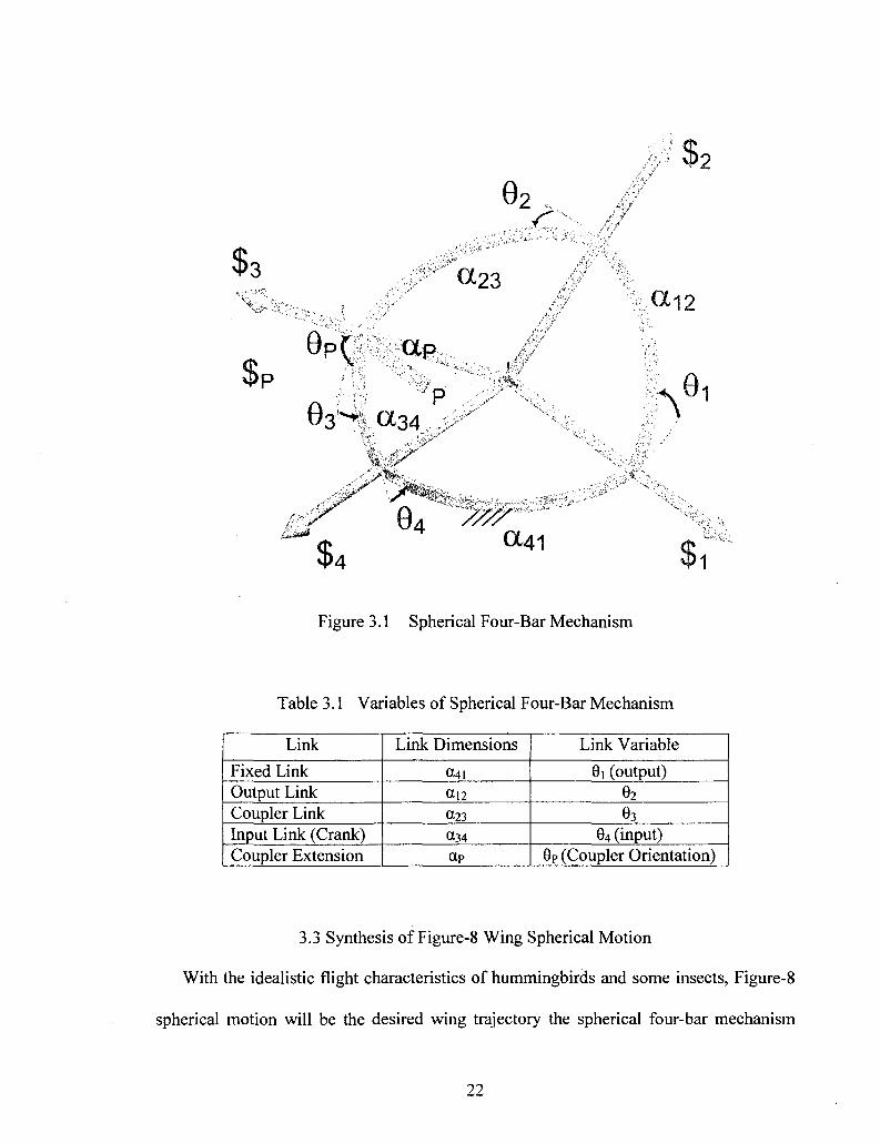
desired motion sought. A schematic of the spherical four-bar mechanism is shown in
Figure 3.1. Table 3.1 lists the variables used to define the variable of spherical four-bar
kinematics based on [26], which contains the fundamental equations based on spherical
four-bar mechanism kinematics.
21
$ :
CD 4>l
0: r:
Ot23
9p^ aP
6: ^ 3 4 , >#
% X >%**
' i*>*
a - ^
$* 0C41
$ ;
a i2
r\°i
Figure 3.1 Spherical Four-Bar Mechanism
Table 3.1 Variables of Spherical Four-Bar Mechanism
Link
Fixed Link Output Link Coupler Link Input Link (Crank) Coupler Extension
Link Dimensions
a4i an a23 a34 ap
Link Variable
0i (output)
e2 63
04 (input) 0P (Coupler Orientation)
3.3 Synthesis of Figure-8 Wing Spherical Motion
With the idealistic flight characteristics of hummingbirds and some insects, Figure-8
spherical motion will be the desired wing trajectory the spherical four-bar mechanism
22

will be designed to accomplish. This motion is similar to what is exhibited by
hummingbirds and some insects capable of high maneuverability and hovering. Figure
3.2 shows the desired wing trajectory the mechanism will be designed to trace. The
motion can be achieved by attaching the wing to the coupler link of the mechanism where
all links are connected by hinge joints. This symmetric Figure-8 requires two planes of
symmetry; therefore, the spherical four-bar mechanism link dimensions and configuration
must be defined accurately to outline the correct coupler path. A crank-rocker spherical
mechanism will provide the suitable configuration to generate this motion.
(cixtcr of spherical motion)
i'8 Cycle
Figure 3.2 Wing Point Trajectory and Induced Velocity
3.3.1 Figure-8 Symmetry Conditions
Certain conditions are required to generate a Figure-8 coupler point curve with two
planes of symmetry. The conditions are outline below.
23

• Condition 1: The mechanism should satisfy Grashof criterion noted in Equation
6.1, [27], to be classified as a crank-rocker four-bar mechanism.
s + Kp + q (3.1)
The angular lengths of the shortest link, s, and longest link, /, must be less than
the other two links. With this condition satisfied and the input as the shortest link,
the input link will fully rotate and a crank-rocker spherical four-bar mechanism
will be established.
• Condition 2: The coupler-curve must intersect only once throughout a complete
cycle of the spherical four bar mechanism.
» Condition 3: The coupler-curve must be symmetric around two planes. The link
angular dimension assignments must be assigned cautiously to verify whether the
spherical mechanism is symmetric about the two planes.
» Condition 4: The assize of the curve is maximized.
The conditions noted above must be satisfied to outline the desire coupler-curve. Table
3.2 lists the angular dimensions that are assigned to each link to satisfy these conditions.
The crank, input link, will be fully rotational as it will be driven by an electric motor. The
orientation of the coupler extension, 9p, will be fixed at -90° (9p = -90°) from the coupler
link. The angular dimension of the input link will be chosen at a later time depending the
angular spacing of the coupler-curve preferred.
Table 3.2 Spherical Four-Bar Mechanism Link Angular Dimensions
Fixed Link a-41
90°
Output Link 0.12
90°
Coupler Link 0-23
90°
Input Link a-34
0 < a34 < 90°
Coupler Extension
90°
24

3.3.2 Motion Synthesis of Figure-8 Phases
The dimensions outlined create a symmetrical Figure-8 coupler-curve with a full
rotation of input link, (X34. Four configurations of the spherical four-bar mechanism are
identified utilizing the dimensions assigned for each link to produce the motion desired.
Figures 3.3 to 3.6 show the configuration of the spherical four-bar mechanism at key
positions that create Figure-8 coupler-curve and are explained in detail.
A ^2
JJ12
J . :
-«5b
//// ;>i
Figure 3.3 Spherical Four-Bar Mechanism, 84 is equal to 0°
As shown in Figure 3.3, the mechanism forms a spherical right triangle with 64 = 0°.
Point P is in the $1 and $4 plane and is aP - 0134 away from $4. The same orientation is
held by (X34 and otp. The angle, 02, is equal to 0,34, 02 = (X34, and 61 = 63 = 0°. This
configuration of the spherical mechanism corresponds to the initial and ending position of
the Figure-8 cycle as shown in Figure 3.2.
25

3 S n?
1 •
. Q.42
r
1"
6C ////'
^ 1 vp
Figure 3.4 Spherical Four-Bar Mechanism, 64 is equal to 90°
When 04 = 90°, point P is along $1 when 83 = 0° as shown in Figure 3.4. The angle, 9i, is
equal to a.34, 61 = 034, and 02 = 90°. A spherical right triangle is formed by 0134, (X41, and ap.
The orientation of P with respect to $i-$4 can be determined using law of cosines for
spherical triangles, [30], as indicated in Equations 3.2 and 3.3.
cos(8) = cos(a34)sin(90°) (3.2)
8 = a34 (3.3)
The angle 8 is determined to be (X34, 5 = 0134. This configuration of the spherical
mechanism corresponds to quarter-cycle position of the Figure-8 trajectory as shown in
Figure 3.2
26
'4
01
"1&®88§?
23 I
c41 ////
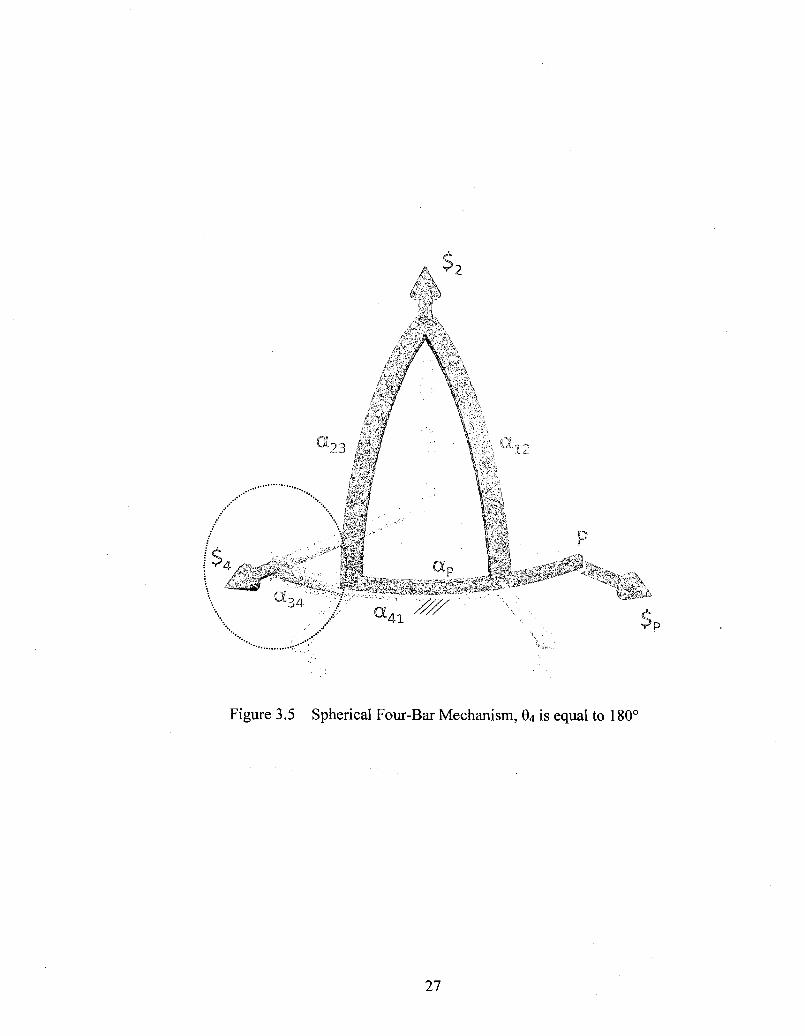
Figure 3.5 Spherical Four-Bar Mechanism, 84 is equal to 180°
27

The mechanism forms another spherical right triangle, Figure 3.5, when 64 = 180°;
therefore, point P is in the $(-$4 plane and ap + (X34 away from $4. The same orientation is
held by a34 and aP. The angles formed are 9i = 90°, G3 = 90°, and 82 = 90° + a34. This
configuration corresponds to half-cycle position of the Figure-8 trajectory as shown in
Figure 3.2.
a 2 3 , / / /
• " . * •
^34
^ 4 ] //// 6"c; * i ,^p
Figure 3.6 Spherical Four-Bar Mechanism, 84 is equal to 270°
When the 04 - 270°, point P is along $1 when 83 = 180° as shown in Figure 3.6. The
angle, 8,, is equal to a34 plus 90°, 8, = a34 + 90°, and 82 = 90° and 84 = 270°. A spherical
right triangle is formed by 034, 041, and aP. The orientation of P with respect to $i-$4 can
be determined using law of cosines for spherical triangles, as indicated in earlier in
28

Equations 3.2 and 3.3, 8 = (X34. This configuration of the spherical mechanism
corresponds to three-quarter cycle position of the Figure-8 trajectory as indicated in
Figure 3.2.
3.4 Resulting Figure-8 Spherical Motion
The resulting coupler-curve is symmetric around the plane of fixed link and the center
of the sphere. The curve is spaced 0134 degrees from either side of $j. At these two
extremities, ap is oriented with the $r$4 plane. Its orientation at the middle of the Figure-
8 is equal to a.34. Figure 3.7 shows the motion of the four-bar mechanism and the path of
the coupler point. By attaching the wing to point P with the same orientation of ap,
Figure-8 motion of the wing can be achieved as can be seen in Figure 3.8. The equations
of motion of spherical mechanism are based on [26] and are listed in Appendix A. A
value of 45° is chosen for 0:34, which results in 90° angular spacing of the wing motion.
29

Crank
N
'N
^ « < * , % , 0
% .
\jf
W M l * -5'°' J " / ' l i l ' * i * _» *P * r & ^ I") % {
/ •
/ : •
Y - Axis 0.5
\ 0.8 0-6 0.4 0-2 .0.2 J)-4 ^-6 JJ-8
X - Axis
Figure 3.7 Motion of the Spherical Four-Bar Mechanism
30

Figure 3.8 Wing Trajectory with Center of Gravity
31

CHAPTER 4
MECHANICAL DESIGN PROCESS
4.1 Objective
With the established idea of creating a wing mechanism using a spherical four-bar
mechanism, the design and fabrication of the mechanism and wing must now be
accomplished. This process begins with first identifying the requirements of the
mechanism and wing for testing purposes. Requirements such as the weight, size, and
flapping frequency must all be taken into account prior to any design. The design process
will then begin with first designing a spherical four-bar mechanism and wing that can
accomplish the required tasks. After determining the design's feasibility, the fabrication
process will then enable us to construct the mechanism, wing and any other essential
components to determine its practicability with testing.
4.2 Design Requirements
In order to design our wing prototype, an ideal approach would integrate weight and
size limitations to determine how the design will be fashioned. The intended design
purpose of the wing prototype is to utilize it for miniature unmanned air vehicles, thereby
restricting it to reasonable compact space, nearly 18 - 24 cm square area with minimal
weight is preferred. This will allow for it to be utilized as is in terms of weight and size,
rather than optimized at a later stage. Flapping frequency must also be considered when
32

determining the size and weight of the wing prototype. Hummingbirds and insects flap
their wings at very high frequency of 100 - 200 Hz and a design consisting of sustainable
components for higher flapping frequency can further relieve enhancements that may
need to be made throughout the testing process.
4.2.1 Size Requirement
As mentioned, the application of the wing prototype is for use in conceptual flapping
wing miniature air vehicles (FWMAV) that are capable of high maneuverability, i.e.
hover. The design is be based on the flapping of hummingbirds and small insects, hence
needed to be compact in size to roughly about 18 - 24 square centimeters as mentioned.
Considering this, the spherical four-bar mechanism would be design to occupy a sphere
of approximately 7 - 8 cm in diameter and the wing would be designed to be about 12 -
14 long and 4 cm wide. In accordance with the size requirement noted, the actual size of
the wing prototype will be determined during the design process.
4.2.2 Weight Requirement
The unknown flight characteristics that will verify the capability of using this design
for practical application provides little information to help determine the weight
requirements for this prototype. It would be best to limit weight as best as possible to
increase the potential of producing enough residual net force, lift, that will allow the
prototype to free itself from the ground and minimize power requirements to drive the
mechanism and wing. Therefore, the spherical four-bar mechanism links should all have
limited mass in terms of design optimization rather than material use. Ideal mass for the
mechanism would be approximately 60 - 70 grams. The wing should also be limited in
mass, about 5 - 7 grams, and not made of metal, but other material that will reduce
33

fabrication time. The minimal mass of the links and wing can further permit us to choose
a lighter motor that is capable of driving the finished prototype and load cell to limit the
overall mass of the prototype.
4.2.3 Flapping Frequency Requirement
The flapping wings of hummingbirds and insects yield unmatched flight ability, thus
provokes the idea presented in this thesis. However, the frequency at which they flap
their wings, approximately 100 - 200 Hz, complicates the design process. This frequency
range seen in nature is very difficult to replicate and requires a perfected design that can
recreate the motion initially. The spherical four-bar mechanism design that is proposed
for our prototype will be conceptual and will attempt to verify the wing motion and flight
characteristics. The design of this prototype, mechanism and wing, will seek to
accomplish testing frequencies starting at 2.5 Hz and reaching the highest frequency
attainable. The inertia driven by the motor will play a vital role in determining the
maximum frequency reached, so limiting the mass of the mechanism and wing will be an
essential guideline during the design process.
4.3 Spherical Four-Bar Mechanism Design
4.3.1 Design
Designing a spherical four-bar mechanism requires careful attention as compared to
planar mechanisms as they reckon to be more challenging. The proper function of a
spherical four-bar mechanism is dependent on many key issues that must be considered
during the design and fabrication process. First, spherical four-bar mechanism links must
be designed to avoid any interference amongst all links. All the links cannot occupy
34

space on the same greater sphere; otherwise they are bound to interfere. Second, in
connecting all links there must be sufficient clearance between each link to allow
unobstructed motion. Lastly, the four axes associated with the joints must intersect at the
center of the sphere or at the same point. If these links do not have a common center
point, the mechanism will lose its mobility by not be able to perform the required task.
To avoid these issues, we begin designing the spherical four-bar mechanism with
each link occupying a space between two concentric spheres within the overall
mechanism sphere. Additionally, spacers are used to between link connections and
occupy space within a sphere similar to the mechanism links. These spacers allow for
unobstructed motion of the mechanism and limit wear associated with continuous motion.
Table 4.1 displays the inner and outer concentric spherical radii of each link and Figure
4.1 shows the space each link occupies within the mechanism sphere.
All of the spherical four-bar mechanism links are designed to maintain weight
balance with minimal mass to provide smooth transmission of the mechanism. Weight
balance is achieved by elongating the crank and output link by 15° and 30° respectively
from the fixed link end. Mass optimization of the coupler and output is accomplished by
reducing the outer ends of both links enough to maintain a balance between mass and
structural stiffness. A base to hold the motor is designed to occupy the space of the fixed
link. The coupler is designed as one piece and occupies the outermost sphere to allow
unobstructed wing motion. Each link is designed to have flat surfaces instead of radial
surfaces, feet, for easier connection, [31]. The proposed design of the spherical four-bar
mechanism is shown in Figure 4.2. The hinge joints of the crank and output link indicate
the connection to the base instead of a fixed link. Also seen in the Figure, the crank and
35

output links are placed on the same sphere as the chosen dimensions ensure that they do
interfere.
Table 4.1 Mechanism Links Concentric Spherical Radii
Link Fixed Link Output Link Crank Coupler Link
Inner Radius -
25 mm 25 mm 31mm
Outer Radius 24 mm 30 mm 30 mm 36 mm
Figure 4.1 Location of Each Mechanism Link amongst the Greater Sphere
36

Fixed Hinges
Figure 4.2 Proposed Conceptual Design of Spherical Four-Bar Mechanism
4.3.1 Fabrication
The conceptual nature of the spherical mechanism prototype did not restrict us to
choose a particular metal in order to limit weight and increase strength. Utilizing metal
instead of creating ABS plastic parts with a rapid prototyping machine would provide
better insight on mechanism's feasibility in exploring potential flapping wing UAV
application. Therefore, the links of mechanism were machined using high strength
Aluminum, 7075, to provide a combination of limited mass and structural stiffness.
Aluminum is an easier metal to machine and is readily available. For easier connection
between all links, they are machined to have flat surfaces on both ends of the hinge
locations. The coupler link is machined as one piece with filleted edges where the
coupler-extension extends from the coupler link. Three counter bore holes are machined
in the base to so that it may be attached to a testing platform. Figure 4.3 shows the actual
machined links used for the prototype of the spherical mechanism and Table 4.2 lists the
37

mass of each link and base. The design and fabrication of these links is accomplished
with careful inspection to limit any complications with prototype testing that would
necessitate a re-design of any link.
G©ypler Li
J
1 • 1 "*
\
* \ _ ^
-
s a
^ " -
JT
•%>.
Figure 4.3 Machined Links Used to Construct Spherical Four-Bar Mechanism
Table 4.2 Mass of Links and Assembly Components for Mechanism
Part Crank Output Coupler Base Brass Sleeve Aluminum Washer Steel Rivet Teflon Ring
Mass (g) 4.60 5.81 15.15 31.00 0.11 0.13 0.62 0.15
38
4.4. Wing
4.4.1 Design
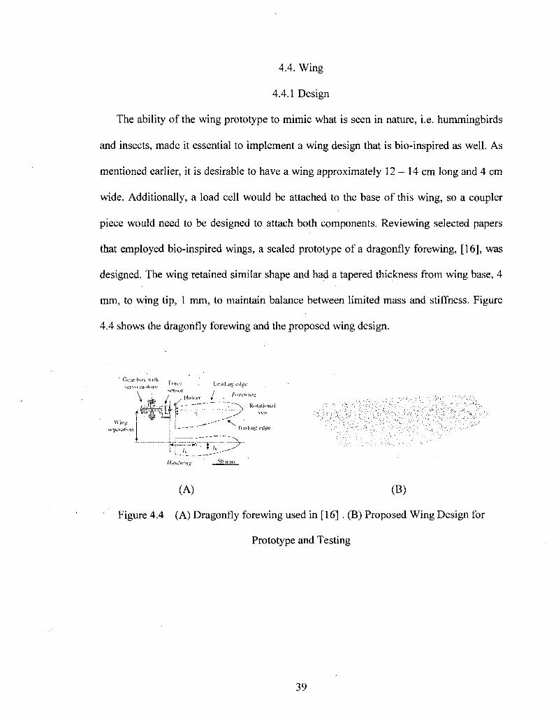
The ability of the wing prototype to mimic what is seen in nature, i.e. hummingbirds
and insects, made it essential to implement a wing design that is bio-inspired as well. As
mentioned earlier, it is desirable to have a wing approximately 12 - 14 cm long and 4 cm
wide. Additionally, a load cell would be attached to the base of this wing, so a coupler
piece would need to be designed to attach both components. Reviewing selected papers
that employed bio-inspired wings, a scaled prototype of a dragonfly forewing, [16], was
designed. The wing retained similar shape and had a tapered thickness from wing base, 4
mm, to wing tip, 1 mm, to maintain balance between limited mass and stiffness. Figure
4.4 shows the dragonfly forewing and the proposed wing design.
Himhnns; 5»-inni
(A) (B)
Figure 4.4 (A) Dragonfly forewing used in [16] . (B) Proposed Wing Design for
Prototype and Testing
39

4.4.2 Fabrication
Mass of our wing was an essential factor that played into the fabrication process.
Initially it was decided to have the wing created using the rapid prototype machine with
ABS plastic. The wing was designed to have cut outs to reduce mass and look similar to a
wing membrane as seen in nature and covered with two Mylar sheets on both ends.
However, the significant mass of this configuration of 9 grams would increase power
required to drive the wing prototype and increase inertial forces acting on the load cell.
The idea of using model grade balsa wood was then investigated to minimize mass. A
wing was cut from a 3/16 inch thick sheet of model grade balsa and sanded on both ends
for a tapered thickness similar to the conceptual design with a mass of 2 grams. It was
reinforced at the shoulder where it would be attached to the wing coupler with three
alternating layers of unidirectional carbon fiber. An ABS plastic coupler was printed
using a rapid prototyping machine for wing and load cell attachment. Figure 4.5 is a top
view drawing of the wing outlining the dimensions and center of gravity, which is located
60.4 mm from the edge of the adapter and 20.3 mm from bottom lower edge of wing. The
total mass of the wings with all components is 3.2 grams.
^ 138 mm - » •
Figure 4.5 Wing Top View
40

4.5 Prototype
The final stage of the design and fabrication process provided the most complexity as
putting together a working wing prototype required careful and proper attachment of all
components. The spherical four-bar mechanism demanded significant attention in making
sure all links would stay in place, provided adequate testing times, and prototype
longevity. This iterative process leads through various ways of making sure a working
prototype was attained. The use of pins, combination of shoulder screws and plastic nuts
with nylon inserts, and aluminum rivets, were options that were tried in an attempt to
make the mechanism yield the results needed. For the final prototype, steel rivets are used
as pins to connect all the links of the mechanisms. To avoid wear and reduce friction,
each link joint is fitted with brass sleeves and then Teflon rings are placed between the
rivet head and link surface. Washers are used as spacers to separate links at hinge
locations and reduce friction as well. Figure 4.6 shows the assembled spherical four-bar
mechanism. As shown, a set crew is used to ensure that the motor shaft remains attached
to the crank and three screws hold it to the base.
41

Actual Pratotjfps ©If Spherical [yfeehanssns
Figure 4.6 Conceptual and Actual Prototype of Spherical Four-Bar Mechanism
For the wing, the plastic wing coupler is attached to the wing shoulder using high
strength epoxy. Three screws applied from both mechanism coupler and wing coupler
ends to the tooling and mounting ends respectively to hold the ATI Nano 17 load cell,
[32]. Figure 4.7 displays and identifies the components of the wing coupler assembly.
Figure 4.8 and 4.9 show a drawing and a photo of the assembled Figure-8 Spherical
Four-Bar mechanism wing prototype respectively.
42

Coupler = 90°
Carbon Fiber Reinforcement
Balsa Wing
Load Cell Load Cell/Wing Coupler
Figure 4.7 Wing Design for the FWMAV Prototype
,w4r̂ ' ^^^^^^-^i^Trjrrm^
Figure 4.8 Figure-8 Spherical Four Bar Mechanism
t S H C -
-LitiH^-i'*
Figure 4.9 Prototype of the Figure-8 Spherical Four Bar Mechanism
43

CHAPTER 5
PROTOTYPE TESTING
5.1 Objective
Wing trajectory is essentially the basis of this design process and must be verified to
determine the mechanism's feasibility. To conduct experimentation for design validation,
prototype testing is conducted to validate to wing motion and generate force signals that
are produced at various flapping frequencies.
5.2 Prototype test Stand/Platform
Proper placement was vital in achieving unobstructed motion of our wing prototype.
In essence, a platform was needed to which we could attach our spherical four bar
mechanism and conduct experimentation. The platform was designed using a quarter inch
aluminum rod threaded into a.three square inch aluminum plate. This aluminum plate was
then attached to a larger aluminum base to hold the rod and smaller plate in position and
placed onto a table. To decouple the table and prototype platform, rubber silicone pads
were glued to the bottom surface corners of the large aluminum base plate to minimize
any vibration associated with ambient disturbances present in the laboratory.
Additionally, an aluminum column was placed over the rod to mitigate vibration
produced by the flapping wing. To attach the base of the wing prototype, a threaded
aluminum coupler piece was attached to the top end of the rod. The base of the UAV
44

prototype was secured using three screws to the coupler piece. Figure 5.1 shows the test
stand platform as described. With this setup, the prototype will sit 42 cm above the main
aluminum base.
Figure 5.1 Wing Prototype Test Stand
5.3 Apparatus/Hardware
Successful experimentation of our wing prototype required proper hardware and
apparatus to establish whether the wing motion could be achieved and identify the forces
it produced. To drive the spherical four bar mechanism, a motor with sufficient power
output was selected. Prior to the selection process, torque, power, and size requirements
45
were identified to understand what type of motor and its power output would be needed.
The mechanism would be driven at lower to higher speeds; therefore, a sensor capable of
detecting very small forces, around 0.5 - 4 N, with a reasonable resolution would provide
the best results. The ATI-IA Nano 17 F/T load cell, [32], provided the best option with its
compact size an ability to resolve down to 0.319 grams. A detailed description of both
components is provided.
5.3.1 Six-Axis F/T Load Cell
Visualization of the forces and moments induced by the Figure-8 motion was possibly
only with a Force/Torque load cell that was capable of generating the experimental force
and moment signal. ATI-IA Nano 17 Force-Torque load cell, [32], is a six axis transducer
with varied range depending on the calibration assignment. The load cell has a high
signal to noise ratio with the use of silicon strain gages rather than conventional foil
gages providing stronger signal. For our application, two calibrations were used which
allowed measurement of up to 17 N and 35 N in the axial direction of the sensor, Fz, with
fine resolution as low as 1/320 N. Table 5.1 list the maximum allowable force per
direction and resolution with regard to the calibration. The sensor will be attached to the
base of the wing to eliminate the need for force transformation.
46

Table 5.1 ATI-IA Nano 17 Load Cell Calibrations
Force Direction
Fx
Fy Fz
Mx
Mv
Mz
Calibration I (FT7863, FT8964)
Maximum Force/Torque
25 N 25 N 35 N
250 N-mm 250 N-mm 250 N-mm
Resolution
1/160 N 17160 N 1/160 N 1/32 N 1/32 N 1/32 N
Calibration II (FT7862,FT8963)
Maximum Force/Torque
12N 12 N 17N
120 N-mm 120 N-mm 120 N-mm
Resolution
1/320 N 1/320 N 1/320 N 1/64 N 1/64 N 1/64 N
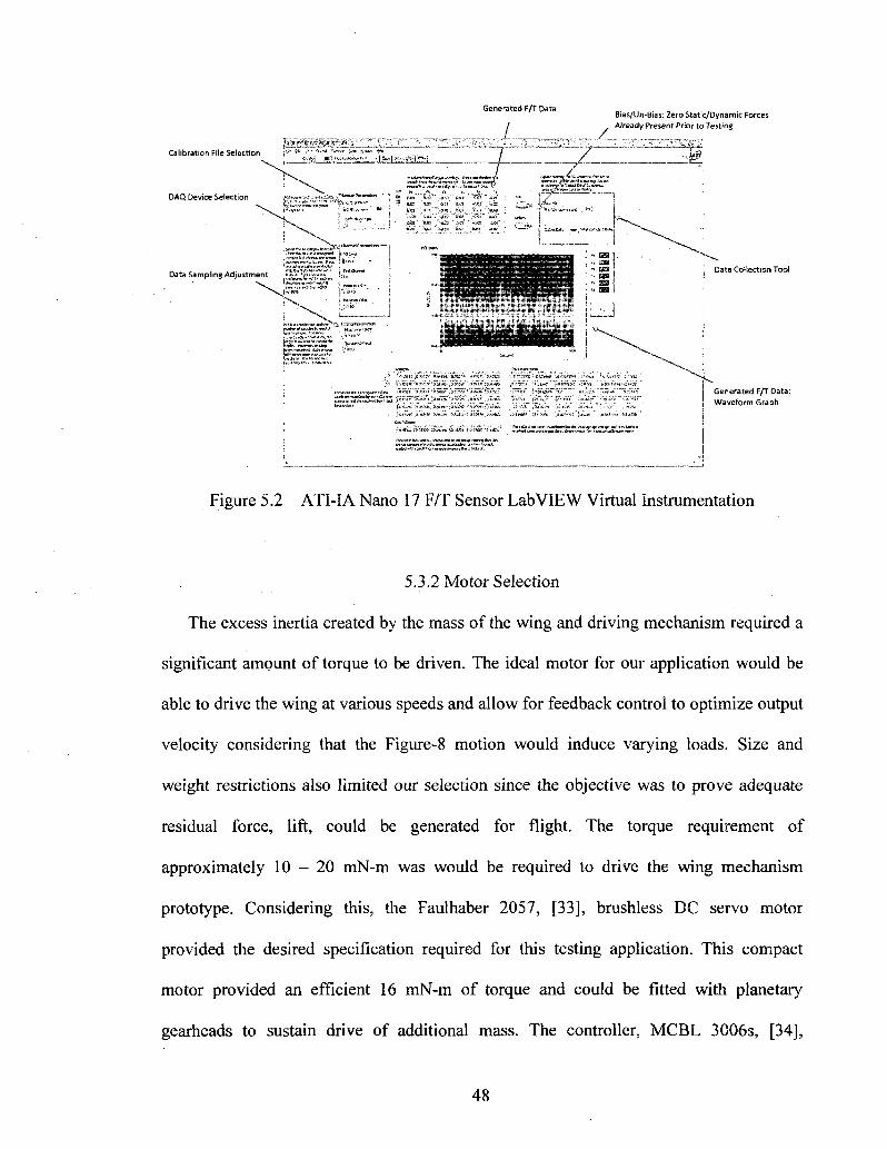
For data acquisition, the ATI Nano 17 requires a NI-DAQ PCI board that is
connected to the signal conditioner. It is connected to the signal conditioner interface and
data is collected using a LabVIEW virtual instrumentation file that has been pre
programmed to accept the sensor outputs. The user is required to select a calibration,
DAQ PCI device number, and determine if static forces applied are to be zeroed prior to
any testing. Data files are generated by LabVIEW as plain text and can be can be
converted to any compatible file for data analysis. Data is sampled at a default 10 kHz,
but can be sampled at lower frequencies if needed. Figure 5.2 shows a screenshot of the
actual LabVIEW virtual instrumentation and outlines the features described.
47
Calibration File Selection i l * !*-' "" 6-*' ^ ' ^ Ia* B ^ »*
DAQ Device Selection
Generated F/T Data
X Bias/Un-Bias: Zero Static/Dynamic Forces Already Present Prior to Testing
Data Sampling Adjustment jSS&i^/??' Data Collection Tool
Generated F/T Data:
Waveform Graph
Figure 5.2 ATI-IA Nano 17 F/T Sensor LabVIEW Virtual Instrumentation
5.3.2 Motor Selection
The excess inertia created by the mass of the wing and driving mechanism required a
significant amount of torque to be driven. The ideal motor for our application would be
able to drive the wing at various speeds and allow for feedback control to optimize output
velocity considering that the Figure-8 motion would induce varying loads. Size and
weight restrictions also limited our selection since the objective was to prove adequate
residual force, lift, could be generated for flight. The torque requirement of
approximately 1 0 - 2 0 mN-m was would be required to drive the wing mechanism
prototype. Considering this, the Faulhaber 2057, [33], brushless DC servo motor
provided the desired specification required for this testing application. This compact
motor provided an efficient 16 mN-m of torque and could be fitted with planetary
gearheads to sustain drive of additional mass. The controller, MCBL 3006s, [34],
48
provided PI feedback control for optimization of velocity control. This 12 volt motor
required a standalone power supply that can supply a constant 12 volts and current of up
to 10 amperes.
5.4 Testing
5.4.1 Motor Control Optimization
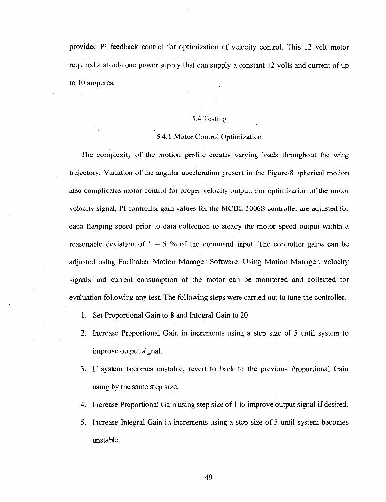
The complexity of the motion profile creates varying loads throughout the wing
trajectory. Variation of the angular acceleration present in the Figure-8 spherical motion
also complicates motor control for proper velocity output. For optimization of the motor
velocity signal, PI controller gain values for the MCBL 3006S controller are adjusted for
each flapping speed prior to data collection to steady the motor speed output within a
reasonable deviation of 1 - 5 % of the command input. The controller gains can be
adjusted using Faulhaber Motion Manager Software. Using Motion Manager, velocity
signals and current consumption of the motor can be monitored and collected for
evaluation following any test. The following steps were carried out to tune the controller.
1. Set Proportional Gain to 8 and Integral Gain to 20
2. Increase Proportional Gain in increments using a step size of 5 until system to
improve output signal.
3. If system becomes unstable, revert to back to the previous Proportional Gain
using by the same step size.
4. Increase Proportional Gain using step size of 1 to improve output signal if desired.
5. Increase Integral Gain in increments using a step size of 5 until system becomes
unstable.
49

6. If system becomes unstable, revert to back to the previous Integral Gain using by
the same step size.
7. Increase Integral Gain using step size of 1 to improve output signal if desired.
Depending on the speed, these steps reduced deviation resulting in limited angular
acceleration which may have corrupted the measured force signal data. Table 5.2 lists
gain values used for the wing prototype at the testing speeds indicated.
Table 5.2 PI Controller Gains at Different Wing Flapping Frequency
Flapping Frequency
(Hz)
2.5 5.0 7.5 10.0
12.25
Motor Command Velocity (RPM)
150 300 450 600 735
PI Controller Proportional
Gain
10 10 11 11 12
Integral Gain
60 50 50 50 50
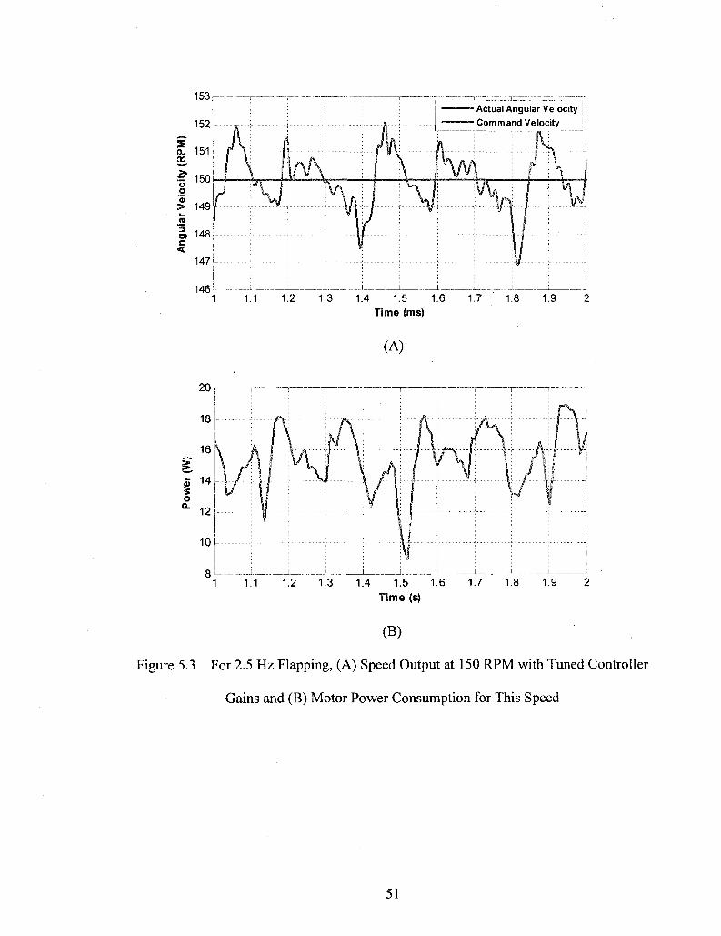
From the current consumption of the motor and the voltage of the power supply, the
relationship between the power required for each testing speed can be made using
Equation 5.1.
p{t) = v(tyn?) (5.1)
The current consumption, i(t), is obtained for each test during testing. The velocity signal
and power required to drive the wing prototype at speeds of 2.5, 5, 7.5, 10 Hz, and 12.25
Hz, are shown in Figures 5.3, 5.4, 5.5, 5.6, and 5.7 respectively.
50
153
152
? OL ac
ity
o o (1)
> « §> c <
1M
150
149
148
147
146
I " r- - - i
1
J " - —
i
Actual Angular Velocity Com mand Velocity
{ j f\ 1 "^j p^
iy 1
i ! 1.1 1.2 1.3 1.4 1.5 1.6 1.7 1.8 1.9
Time (ms)
(A)
20
18
16
fc 14 o °- 12
10
8
1 1 1 i 1 i - • i i — -
__i ! L i i i 1 L I 1 1.1 1.2 1.3 1.4 1.5 1.6 1.7 1.8 1.9 2
Time (s)
(B)
ure 5.3 For 2.5 Hz Flapping, (A) Speed Output at 150 RPM with Tuned Controller
Gains and (B) Motor Power Consumption for This Speed
51
Actual Angular Velocity Command Velocity
1.4 1.5 1.6 Time (ms)
(A)
(B)
Figure 5.4 For 5 Hz Flapping, (A) Speed Output at 300 RPM with Tuned Controller
Gains and (B) Motor Power Consumption for This Speed
52

460 Actual Angular Velocity Command Velocity
1.4 1.5 1.6 Time (ms)
(A)
(B)
ure 5.5 For 7.5 Hz Flapping, (A) Speed Output at 450 RPM with Timed Controller
Gains (B) Motor Power Consumption for This Speed
53

615 Actual Angular Velocity Command Velocity
(A)
1.1 1.2 1.3 1.4 1.5 1.6 1.7 1.8 1.9 Time (ms)
(B)
Figure 5.6 For 10 Hz Flapping, (A) Speed Output at 600 RPM with Tuned Controller
Gains and (B) Motor Power Consumption for This Speed
54

760 • Actual Angular Velocity ' Command Velocity
1.4 1.5 1.6 Time (ms)
(A)
I
2
(B)
Figure 5.7 For 12.25 Hz Flapping, (A) Speed Output at 735 RPM with Tuned
Controller Gains and (B) Motor Power Consumption for This Speed
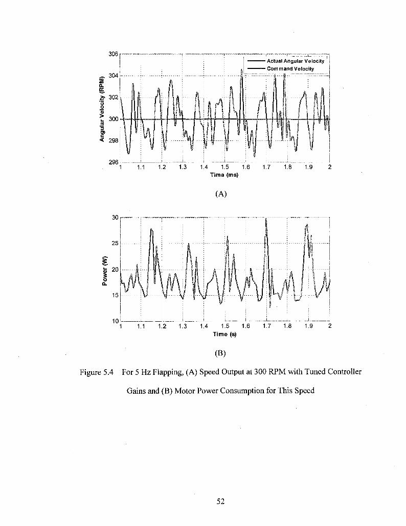
5.4.2 Pre-Testing Conditions
Once the motor has been configured to provide the adequate speed control at the
testing velocity, the wing prototype should be ready for testing. The prototype is aligned
55
to the initial position of the Figure-8 as indicated in Figure 5.8 and the load cell forces are
zeroed to ignore any static effect present at that time. With the load cell attached to the
base of the wing, the coordinate frame as shown in Figure 5.8 is assigned. The position of
the load cell is set to this position to avoid interference with the load cell cord. The
prototype is then set in motion and data is collected for typical testing time of about 6 -
12 seconds. Although the wing prototype is aligned to the initial position of the Figure-8,
no such requirement is made for the position where it must stop. An explanation of the
force signal produced during motion is examined later in this chapter.
Figure 5.8 Wing Prototype at the Initial Position of Figure-8 with Load Cell Attached
and Coordinate Frame Assigned
5.5 Data Analysis
5.5.1 Filtering
Acquired experimental force signals contain significant noise that contaminate the
data and must be removed to interpret the forces produced during testing. Using Fast
56

Fourier Transform technique for digital signal processing, the dominate frequencies of
the acquired data signal are classified. Higher order frequencies are eliminated from the
data using a Butterworth low pass filter. Depending on the testing frequency, the cutoff is
typically 25 - 50 Hz. A Butterworth filter provides the most efficient filter for this
application by generating smooth curves for the given data. All six force components are
filtered and verified for accuracy. The moving average of the collected data is also taken
at times using 250 - 500 samples for additionally information on the values and trend of
each component.. The data corresponding to prototype testing will be filtered and a more
detailed analysis will be provided in Chapter 7. The results of prototype testing and
comparisons with model results will be provided in Chapter 7 as well.
5.6 Force Signal Interpretation
Interpreting the measured force signal involves understanding the phase during the
Figure-8 cycle a directional force is present and when it should peak. Since our data has
shown consistency over all flapping frequencies, reasoning of the of the axial force, Fx,
and normal force, Fy, is explained in the Figures below.
5.6.1 Chord-wise Force, Fx, Interpretation
The chord-wise force, Fx, induced by the Figure-8 wing motion represents dynamic
and drag forces as the wing moves through air. The wing phases are divided into sections
and reasoning for the measured force signal is provided, Figure 5.9. Since the load cell is
attached the base of the wing, forces induced by the movement of the wing through its
motion cycle are the only contributing factors to the signal.
57

I
1 1.01 1.02 1.03 1.04 1.05 1.06 1.07 1.08 1.09 1.1 Time (s)
Figure 5.9 Chord-wise Force, Fx, Representation for Figure-8 Cycle
A. Initial Position: Wing Prototype is aligned horizontally initially prior to testing. At
this location, A, the load cell is zeroed to eliminate any static load present.
Although, the load cell is zeroed, the load cell does not assume the same for
dynamic forces. This position does represent the maximum position along the
positive chord-wise direction according to the Figure-8 trajectory. Therefore, Fx,
is reaches its max value at this position. The angle of attack during this phase is
90°.
B. Quarter Cycle: During this phase, the wing is slicing through the air with angle of
attack of 0° transitioning to the other half of the Figure-8 trajectory. At this
position, B, the wing is half way from its maximum and minimum along the
chord-wise direction. Additionally, maximum acceleration is likely present at
58

section; therefore, it is zero at this location and transitioning to its opposite
amplitude peak.
C. Half Cycle: The wing trajectory has reached it opposite maximum end along the
chord-wise direction. This position represents the same magnitude opposite
direction to the initial position.
D. Three-Quarter Cycle: Similar to position B, this wing is now moving in the
opposite direction, hence Fx is zero.
E. Full Cycle: Reaches back to initial position where Fx is maximum.
5.6.2 Normal Force, Fy, Interpretation
The normal force, Fy, induced by the Figure-8 wing motion also represents dynamic
and lift forces as the wing moves through air. Similarly, the wing phases are divided into
sections and reasoning for the measured force signal is detailed below and shown in
Figure 5.10.
"l 1 i r
I I " T — — » i I I " - — — I ™ " I I I I 1 1.01 1.02 1.03 1.04 1.05 1.06 1.07 1.08 1.09 1.1
Time (s)
Figure 5.10 Normal Force, Fy, Representation for Figure-8 Cycle
59

A. Initial Position: Wing Prototype is aligned horizontally initially prior to testing. At
this location the normal force, Fy, is zero.
B. Eighth Cycle: During this phase, the wing is up-stroking stroking as the angle of
attack is decreasing from 90°. Fy reaches is first peak at this position.
C. Quarter Cycle: The wing is half way from transitioning from its first and second
peak. As it reaches 0° angle of attack and is coincident with the stroke-plane or
axis of symmetry along the Figure-8, Fy is zero.
D. Three-Eighth Cycle: Fy is again maximum as it reaches its opposite amplitude
peak during the first half of the Figure-8 cycle. During this phase it is
transitioning from 0° to 90° angle of attack.
E. Half Cycle: Fy is zero similar to initial position, it is coincident and parallel to the
Figure-8 stroke plane and axis of symmetry.
As shown in the figure and indicated in the Figure-8 trajectory, double peaks are present
in the Fy force. From position E, Fy will again oscillate from maximum to minimum
during the second half of the Figure-8 cycle until it reaches its initial position.
5.6 Motion Verification
The validity of the design and collected force signal is dependent on whether proper
motion trajectory is achieved by the wing prototype. The use of the spherical four-bar
mechanism with the angular dimensions assigned to each link will allow the coupler to
outline a two plane symmetrical Figure-8 coupler curve. However, it is essential to verify
the motion trajectory of the prototype for surety of test results and that the design
objective as outline in Chapter 3 is met. Still and high speed video imagery is used to
60
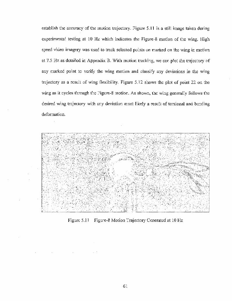
establish the accuracy of the motion trajectory. Figure 5.11 is a still image taken during
experimental testing at 10 Hz which indicates the Figure-8 motion of the wing. High
speed video imagery was used to track selected points on marked on the wing in motion
at 7.5 Hz as detailed in Appendix B. With motion tracking, we can plot the trajectory of
any marked point to verify the wing motion and classify any deviations in the wing
trajectory as a result of wing flexibility. Figure 5.12 shows the plot of point 22 on the
wing as it cycles- through the Figure-8 motion. As shown, the wing generally follows the
desired wing trajectory with any deviation most likely a result of torsional and bending
deformation.
Figure 5.11 Figure-8 Motion Trajectory Generated at 10 Hz
61

Figure 5.12 Figure-8 of High Speed Motion Capture of Point 22 of Figure A.2
62

CHAPTER 6
WIND TUNNEL TESTING
6.1 Objective
To realize the potential flight capabilities of Figure-8 spherical motion, the flight
characteristics must be quantified. To achieve this, the lift and drag effects associated
with this wing motion must be identified. As the wing prototype cycles through Figure-8
spherical motion, high angles of attack are reached making it difficult to predict the
behavior of air flow around the wing. The wing is initially positioned 90° angle of attack,
and cycles between 0° to 90° angle of attack throughout the wing trajectory. To
determine the lift and drag experienced by the wing prototype, wind tunnel
experimentation is conducted. The wing is rotated in the wind tunnel at quasi-static and
dynamic conditions. Data is collected as the wing is rotated for a half and full cycle
depending on the type of test, at a wind speed equivalent to the free stream velocity at
about 10 - 12.25 Hz. Using the data collected; we can calculate the coefficients of lift, Q,
and drag, Q , for the complete cycle. Since our wing motion only reaches 90° angle of
attack, data corresponding to this portion of the cycle, 0 - 90° angle of attack, is
interpreted.
63

6.2 Free Stream Velocity and Angle of Attack
During the cycle of Figure-8 motion, the wing is subjected to changes in angle of
attack that needs to be identified to interpret lift and drag variation. For prototype testing,
the wing is stationary, so airflow is assumed to be zero and any fluid movement is a result
of wing motion. Accordingly, we define the free stream velocity, V, of the Figure-8
motion as the velocity induced over the wing acting tangent to the wing trajectory, Figure
6.1. Moreover, the velocity component in the direction of the wing edge is defined as U.
Figure 6.2 displays the velocity interpretation over the wing profile.
(ccctcr of spherical aiotion) l.« Cycle
0. I C 7 *
lactic
lit Cycle
Si* Cycle
Figure 6.1 Wing Point Trajectory and Induced Velocity
Figure 6.2 Free Stream Velocity, V, and Velocity along the Wing Edge, U
64
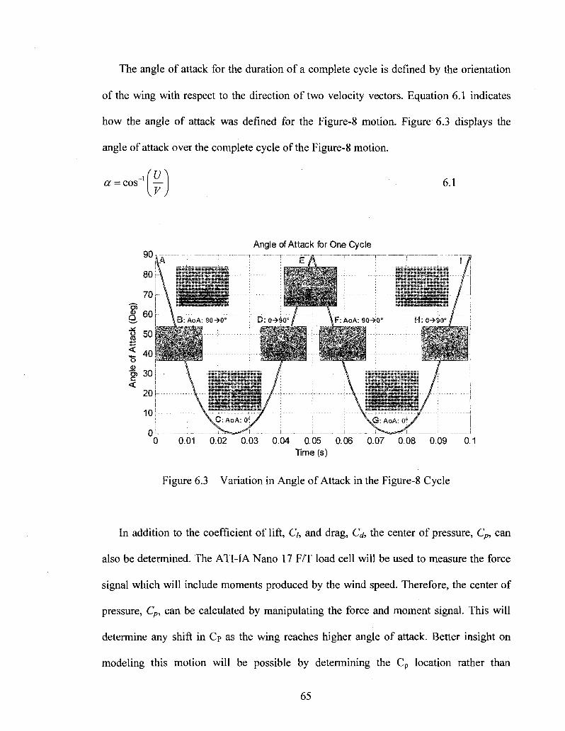
The angle of attack for the duration of a complete cycle is defined by the orientation
of the wing with respect to the direction of two velocity vectors. Equation 6.1 indicates
how the angle of attack was defined for the Figure-8 motion. Figure 6.3 displays the
angle of attack over the complete cycle of the Figure-8 motion.
a = cos - i 6.1
Angle of Attack for One Cycle
0.01 0.02 0.03 0.04 0.05 0.06 0.07 0.08 0.09 0.1 Time (s)
Figure 6.3 Variation in Angle of Attack in the Figure-8 Cycle
In addition to the coefficient of lift, Q, and drag, Cd, the center of pressure, Cp, can
also be determined. The ATI-IA Nano 17 F/T load cell will be used to measure the force
signal which will include moments produced by the wind speed. Therefore, the center of
pressure, Cp, can be calculated by manipulating the force and moment signal. This will
determine any shift in Cp as the wing reaches higher angle of attack. Better insight on
modeling this motion will be possible by determining the Cp location rather than
65

assuming the convention quarter-chord location in accordance with thin air foil theory.
Figure 6.4 shows the assumed location of Cpand the acting aerodynamic forces.
6.3 Setup and Apparatus
To simulate proper wing movement of the wing in the wind tunnel, a setup consisting
of a force/torque load cell, motor, and wing is required. It was desired to have the wing
setup near the center of the wind tunnel mounting area along with the motor and sensor to
rotate the wing and collect data. First a base mount that can be attached to the bottom of
the wind tunnel and support the motor was machined. The DC servo motor, Faulhaber
V2057S0012 with gear reduction of 9.7:1 used for prototype testing and capable of
stepper functions, was attached to the base mount. The load cell was attached to the base
of the wing retaining the coordinate frame as used for prototype testing. The load cell will
rotate with the wing; thereby, eliminating the need force transformation. A coupler piece
is machined to attach the wing and sensor to the motor. Lastly, to limit and disturbances
created by the wind speed which may incorporate erroneous data to the measured force
66
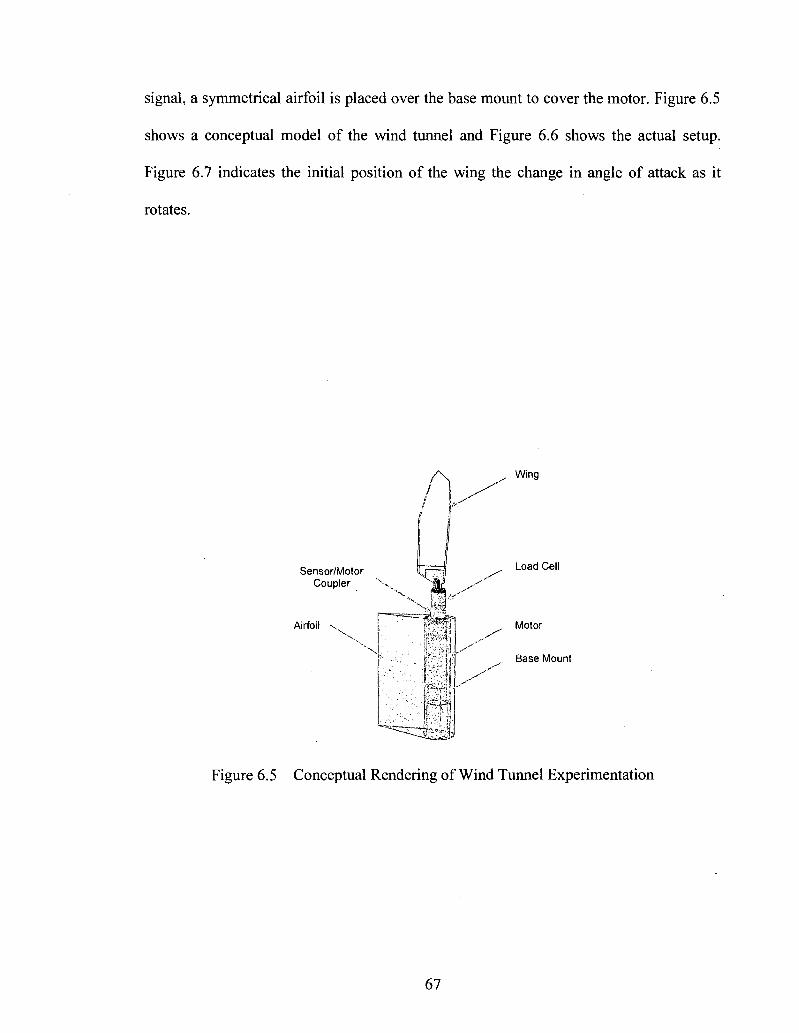
signal, a symmetrical airfoil is placed over the base mount to cover the motor. Figure 6.5
shows a conceptual model of the wind tunnel and Figure 6.6 shows the actual setup.
Figure 6.7 indicates the initial position of the wing the change in angle of attack as it
rotates.
Sensor/Motor Coupler
Airfoil
Load Cell
Figure 6.5 Conceptual Rendering of Wind Tunnel Experimentation
67

r
<
'•#*M- J
Figure 6.6 Wind Tunnel Experimentation Setup
'- 'i
Wind Speed
180°
Change in Arigle of Attack
Figure 6.7 Wing Rotation in Wind Tunnel With Respect to Angle of Attack
68
6.3.1 Setup Conditions
In calculating the coefficients of flight for any given test, certain testing conditions
need to be identified prior to testing. Working with an open circuit wind tunnel, constant
air flow and air properties of the testing environment are essential in obtaining accurate
results. Ambient pressure and temperature readings are needed to calculate the air density
before and during testing. A log of the pressure and temperature was kept for every half
hour starting about two hours before testing to classify any dramatic changes in ambient
conditions. This data was used to calculate the air density using Equation 6.2.
In the equation, R is the gas constant, p is the measured pressure, and T is the measured
temperature. The ambient relative humidity was not considered in pressure calculations
with the assumption of only dry air present.
6.3.2 Motor Control in Stepper Mode
The Faulhaber DC servo motor was to be driven in stepper mode to control the speed
and position of the wing. Using a function generator virtual instrumenOptation program
created in LabVIEW, analog pulse inputs were supplied to the MCBL 30906s controller
from an NI Elvis station to allow rotation as needed. The steps per revolution are freely
programmable by setting two parameters on the motor controller, STW, step width or
number of steps per encoder pulse, and STN, step number or number of steps per
revolution. Both values could be set from 0 to 65,535 depending on the application.
69

6.4 Quasi-Static Analysis
Initial wind tunnel testing was conducted using quasi-static conditions by rotating the
wing slowly at 1.2887 revolutions per minute or about 0.2 Hz. The slow change in angle
of attack provided insight on how airflow affected the wing during static changes in angle
of attack rather than dynamic. The gearhead on the motor made it mechanically difficult
for it to driven at constant angular velocity of 1 RPM; therefore, the motor was
configured to rotate at slightly higher angular velocity of 1.2887 RPM. The step width,
STW, and step number, STN, were set to one and 60,000 respectively enabling the motor
to step 1/60,000 of a revolution or [1.67 10"5]° per pulse input. Table 6.1 lists motor
parameters for this experiment. The wing is rotated from 0 to 180° angle of attack, but
data for only 0 to 90° will be examined since Figure-8 wing motion reaches a maximum
of 90° angle of attack.
Table 6.1 Motor Testing Parameters for Quasi-Static Testing
STN
1
STW
60,000
Frequency (Hz) 250
No. of Revolutions
0.5
No. of Pulses 30,000
Motor Output (RPM) 1.2887
Time Elapsed (s)
23.28
6.4.1 Coefficients of Axial and Normal Force
The measured force signal represents the aerodynamic forces induced by the wind
speed as the wing is rotating in the wind tunnel. Since the load cell is rotating with the
wing, alignment of the x and y axis along the chord-wise and normal direction is
maintained. The coefficients of axial force, Ca, and normal force, C„, can be calculated
70

using Fx and Fy data respectively. First the force signal is filtered at 1 Hz in accordance
with the signal's FFT and then Equations 6.3 and 6.4 are used to calculate Ca and Cn.
C.= . F t (6.3)
C.= . Fy (6.4) \pa,S-s
The density of air, p, is calculated by the ambient pressure and temperature during the
time of testing. The wing surface area, S, is determined using the solid model as designed
in SolidWorks. Table 6.2 list the testing and wing parameters needed for these
calculations. The filtered force signals Fx, Figure 6.8, and Fy, Figure 6.9, are displayed for
this testing. Figures 6.10 and 6.11 display the coefficient of axial force, Ca, and normal
forces, C„, from 0 - 90° for this test respectively. These coefficients are used to determine
the aerodynamic model as outlined in Appendix C.
Table 6.2 Testing Conditions and Parameters for Quasi-Static Testing
Wind Speed (MPH)
10
Wind Speed (m/s)
4.4704
Air Density (p, kg/m3)
1.103867483
Wing Surface Area (S, m2)
0.0040639434
71

0.03 [
0.02
Z 0.01
,'.
-0.01 t-
-0.02
-0.03
Unfiltered -••-- Filtered
0 10 20 30 40 50 60 70 80 90 Angle of Attack (Deg.)
Figure 6.8 Force Signal, Fx, for Quasi-Static Wind Tunnel Testing
0.1 i
0.05
= • 0
1 - 0 . 0 5 ! - - - - • ' • ' - - • ' • , > ' • « *
W;. **#«
"T " t " * * * , *• W ™ w '* ."•'•" ™ *»'""
-0.1 i- Unfiltered Rltered
-0.15!
0 20 40 60 80 100 120 140 160 180 Angle of Attack (Deg.)
Figure 6.9 Force Signal, Fy, for Quasi-Static Wind Tunnel Testing
72
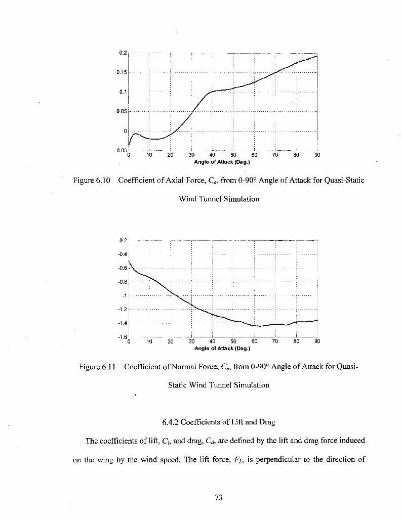
0.2
0.15
0.1
0.05
-0.05 i i i i 1 i : i i _ 10 20 30 40 50 60
Angle of Attack (Deg.) 70 80 90
Figure 6.10 Coefficient of Axial Force, Ca, from 0-90° Angle of Attack for Quasi-Static
Wind Tunnel Simulation
-0.4
-0.6
-0.8
-1
-1.2
-1.4
-1.6 i i i. i i L i i 0 10 20 30 40 50 60
Angle of Attack (Deg.) 70 80 90
Figure 6.11 Coefficient of Normal Force, C„, from 0-90° Angle of Attack for Quasi-
Static Wind Tunnel Simulation
6.4.2 Coefficients of Lift and Drag
The coefficients of lift, C/, and drag, Q , are defined by the lift and drag force induced
on the wing by the wind speed. The lift force, Fi, is perpendicular to the direction of
73

velocity and the drag force, FD, is parallel to the direction of velocity, Figure 6.4.
Therefore, at any angle of attack, a, Q and Cd can be calculated by using transformations
of Ca and C„ with respect to the angle of attack as shown in Equations 6.5 and 6.6.
C, = C„ cos(a) - Ca sin(a) (6.5)
Cd = C„ sin(ar) + Ca cos(a) (6.6)
The change in lift and drag can be seen in Figures 6.12, which displays C/ and Cd over 0
90° angle of attack.
0.8
0.6
0.4
0.2
Coeffiecientof LiftCd
* • - *
j ' : :
1 i i
I J -̂J------
" ^ ^
J i ._ _L_ -. 0 10
Angle of Attack (Deg.)
Figure 6.12 Coefficient of Lift, C/, and Drag, Cd, for 0-90° Angle of Attack for Quasi-
Static Wind Tunnel Simulation
From the change in lift and drag, the following analysis can be made about the
aerodynamic coefficients for the wing at varying angle of attack under quasi-static
conditions.
• Both Ci and Q start from close to zero at 0° angle of attack. There should not be
any lift or drag when the wing is slicing through at the Figure-8 trajectory as
74
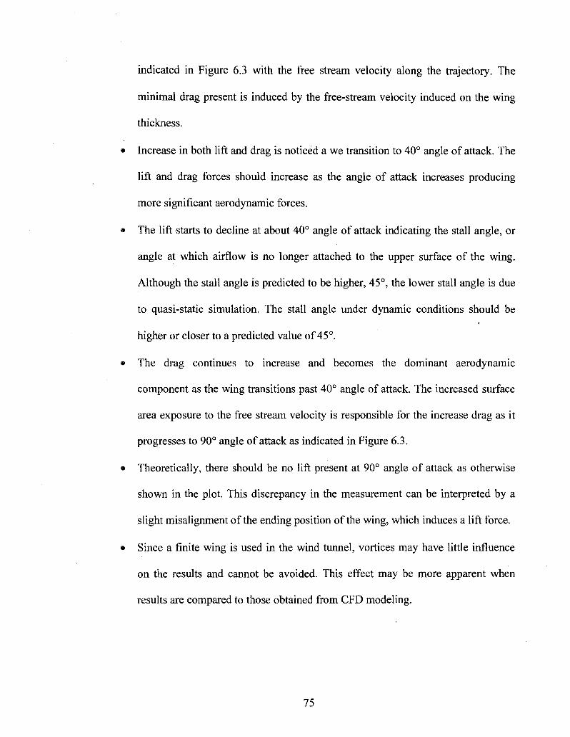
indicated in Figure 6.3 with the free stream velocity along the trajectory. The
minimal drag present is induced by the free-stream velocity induced on the wing
thickness.
Increase in both lift and drag is noticed a we transition to 40° angle of attack. The
lift and drag forces should increase as the angle of attack increases producing
more significant aerodynamic forces.
The lift starts to decline at about 40° angle of attack indicating the stall angle, or
angle at which airflow is no longer attached to the upper surface of the wing.
Although the stall angle is predicted to be higher, 45°, the lower stall angle is due
to quasi-static simulation. The stall angle under dynamic conditions should be
higher or closer to a predicted value of 45°.
The drag continues to increase and becomes the dominant aerodynamic
component as the wing transitions past 40° angle of attack. The increased surface
area exposure to the free stream velocity is responsible for the increase drag as it
progresses to 90° angle of attack as indicated in Figure 6.3.
Theoretically, there should be no lift present at 90° angle of attack as otherwise
shown in the plot. This discrepancy in the measurement can be interpreted by a
slight misalignment of the ending position of the wing, which induces a lift force.
Since a finite wing is used in the wind tunnel, vortices may have little influence
on the results and cannot be avoided. This effect may be more apparent when
results are compared to those obtained from CFD modeling.
75

6.4.3 Center of Pressure
The continuous variation in angle of attack during the course of a cycle in Figure-8
spherical motion is likely to shift the location of the center of pressure, Cp, along the
chord and span length of the wing. With the net aerodynamic forces acting at the Cp, any
aerodynamic moments at this point are zero. Since the load cell is not aligned along the
Cp axis of the wing, a moment signal is incorporated into the data collected. The moment
data can be used to determine the location of Cp with respect to the load cell tooling
surface. Figure 6.13 shows the distance vector, R, defined to calculate the moments
induced by the forces acting on the wing in the wind tunnel. Equations 6.7 and 6.8
indicate the moments acting on the wing.
^^^pSiwise)
•Qfki
R (CP Position Vector) ;
Fy (Normal)
Fx (Axial/Chord - Wise)
Load Cell - Forces and Moments
,y Resolved At Tooling Surface
* T f " , - : - <
, \ * v '; - l i b
Figure 6.13 Cp Position Vector, R, Definition
76

M, = FR - FR
My=FxRz+FRx
K = FyRx-FxRy
(6.7)
0
Fz
F.
Fz _F)
0 Fx
-F . 0
\K K kj
. =
X~ My
Mz
(6.8)
With the tapered wing thickness, 4 mm at the base to 1 mm at the tip, the change in Cp
along the y axis is negligible, thus Ry is zero. Ideally, the span-wise force, Fz, should be
zero given that wind speed will not induce force in that direction; however, this force
may be present in the signal since a finite wing is used for experimentation with effects of
vortices unknown. For Cp calculation purposes, Fz is assumed to be zero. Lastly, My is
also assumed to be zero because of the relatively small wing thickness the forces
producing this moment are applied to. Updating Equation 6.7 with the assumptions
outlined yields Equation 6.9 used to determine the change in Cp along the wing chord-
wise and span-wise direction. Figure 6.14 shows the change in Cp over the angle of attack
for quasi-static testing.
0 -Fy
F, 0 (6.9)
77

120
100
80
E
E. 60
20 h
-20
^ - T - - ! f---- - - -
Rx
— Rz
_ - " _ l " i _ —'
Location Along X (Chord-wise)
Location Along Z (Spanwise)
.'_.'4"_-'-"__"-j._",_"i"_^u_-_--.
i I i i _J i i i
10 20 30 40 50 60 70
Angle of Attack (Deg.)
80 90
Figure 6.14 Change in Center of Pressure, Cp, in Chord-wise and Span-wise Direction
for 0-90° Angle of Attack
The location of center of pressure, Cp can assist in modeling the aerodynamic forces
rather than assuming a conventional quarter-chord location for thin plate airfoil. From the
plot above, the location of Cp shifts along the span-wise direction by initially starting at
100 mm from the load cell tooling surface. The span-wise location steadies after 30°
angle of attack. The chord-wise shift in Cp signifies that quarter chord location is
assumed initially, but deviates to near half chord location at higher angle of attack.
6.5 Dynamic Analysis
Another round of wind tunnel testing was conducted to simulate dynamic change in
angle of attack more accurately representing our prototype testing scenario. Similar to
quasi-static analysis, the wing is rotated in the wing tunnel, full revolution for this test,
and the force signal is examined. The force signal will be used to determine the
coefficients of axial and normal force, Ca and C„, and for coefficients of lift and drag, C/
78

and Cd. For this test, the wing is rotated for a full revolution, 0 - 360° angle of attack, at 1
Hz. The rotation of a complete cycle will eliminate any deceleration force required to
stop the attached wing and load cell assembly which may be incurred if rotated for half a
revolution. This force would distort the data with erroneous information not pertaining to
the actual testing. The DC motor was again configured for use in stepper mode and
provided a step of 0.0005° per pulse input. Table 6.3 lists the motor parameters assigned
for this test and Table 6.4 lists the testing conditions.
Table 6.3 Motor Testing Parameters for Dynamic Testing
STN
1
STW
2,000
Frequency (Hz) 250
No. of Revolutions
1
No. of Pulses 2,000
Motor Output (RPM)
60
Time Elapsed (s) 1
Table 6.4 Testing Conditions and Parameters for Dynamic Testing
Wind Speed (MPH)
10
Wind Speed (m/s)
4.4704
Air Density (p, kg/m3)
1.118301672
Wing Surface Area (S, m2)
0.0040639434
6.5.1 Coefficients of Axial and Normal Force
The coefficient of axial, Ca, and normal force, C„, are calculated for dynamic wind
tunnel simulation similar to quasi-static using Equations 6.3 and 6.4. These coefficients
are incorporated into the model outlined in Appendix C. Figures 6.15 and 6.16 represent
the force signal Fx and Fy for dynamic wind tunnel testing, which is filtered at 10 Hz in
accordance with the FFT. The coefficient of axial force, Ca, and coefficient of normal
force, C„, from 0 - 90° angle of attack are plotted in Figure 6.17 and 6.18 respectively.
79

0.04 r
0.02
„ I ' ' I ' l i ' l ,
Unfiltered
Filtered
-0.02
-0.04
11 ' f i t ' I > ' i i
i' n|ii (i 11
ii,' i i J n ,i
.0.061 1 L 1 i 1 L J 1 0 10 20 30 40 50 60 70 80 90
Angle of Attack (Deg.)
Figure 6.15 Force Signal, Fx, for Dynamic Wind Tunnel Testing
0.1
0.05
-0.05 r
-0.1 '
\ Unfiltered ——— Filtered
;feh-wm^mmu 10 20 30 40 50 60
Angle of Attack (Deg.) 70 80 90
Figure 6.16 Force Signal, Fy, for Dynamic Wind Tunnel Testing
80

0.03
0.02
0.01
-0.01
-0.02
-0.03
-0.04
-0.05 i ! I j ] i i L_ — 0 10 20 30 40 50 60
Angle of Attack (Deg.) 70 80 90
Figure 6.17 Coefficient of Axial Force, Ca, from 0-90° Angle of Attack for Dynamic
Wind Tunnel Simulation
0.5 —
-0.5
-1.5
~~T-\. x
v
- — • *
\
\ - ^ _
i .__ _
':
r—-10 20 30 40 50 60 70 80
Angle of Attack (Deg.) 90
Figure 6.18 Coefficient of Normal Force, C„, from 0-90° Angle of Attack Dynamic
Wind Tunnel Simulation
81
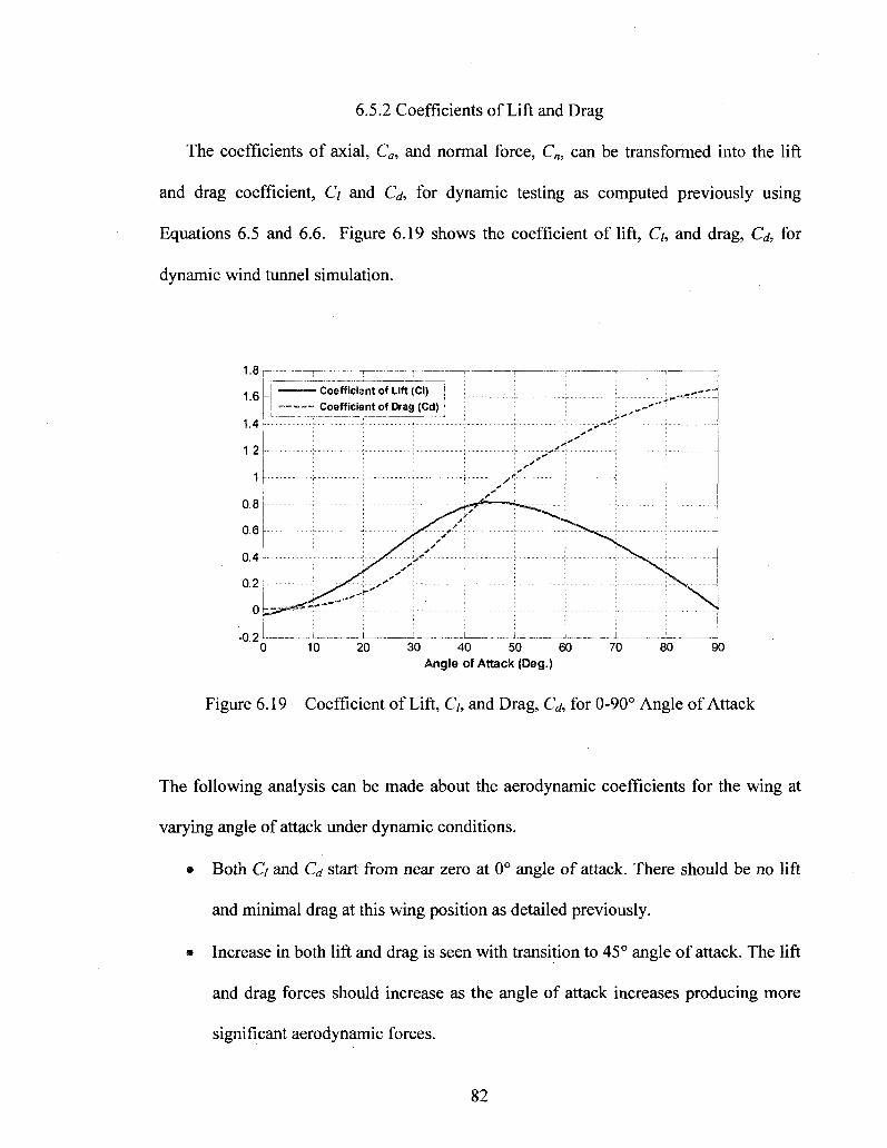
6.5.2 Coefficients of Lift and Drag
The coefficients of axial, Ca, and normal force, C„, can be transformed into the lift
and drag coefficient, Q and Cd, for dynamic testing as computed previously using
Equations 6.5 and 6.6. Figure 6.19 shows the coefficient of lift, Q, and drag, Cd, for
dynamic wind tunnel simulation.
1.8
1.6
1.4
1.2
1
0.8
0.6
0.4
0.2
0
-0.2 0 10 20 30 40 50 60 70 80 90
Angle of Attack (Deg.)
Figure 6.19 Coefficient of Lift, Ch and Drag, Q , for 0-90° Angle of Attack
The following analysis can be made about the aerodynamic coefficients for the wing at
varying angle of attack under dynamic conditions.
• Both Q and Cd start from near zero at 0° angle of attack. There should be no lift
and minimal drag at this wing position as detailed previously.
• Increase in both lift and drag is seen with transition to 45° angle of attack. The lift
and drag forces should increase as the angle of attack increases producing more
significant aerodynamic forces.
82
' Coefficient of Lift (CI)
Coefficient of Drag (Cd)

® The lift starts to plunge into decline at about 45° angle of attack as compared to
40° for quasti-static testing indicating a greater stall angle. The stall angle under
these conditions should is higher as expected because of delayed stall induced by
dynamic change in angle of attack.
• The drag continues to increase and becomes the dominant aerodynamic
component as the wing transitions past 45° angle of attack. The increased surface
area exposure to the free stream velocity is responsible for the increase drag as it
progresses to 90° angle of attack as indicated in Figure 6.3.
• The coefficient range is higher for drag and almost similar for lift for dynamic
testing. Differences in magnitude can be a result of vortices, which are
unavoidable with wind tunnel testing of a finite wing.
6.5.3 Center of Pressure
The calculation of center of pressure, Cp, is made using the same assumptions as
made for quasi-static testing. Using Equation 6.9, the location of CP along the wing span-
wise and chord-wise direction is plotted in Figure 6.20. A discontinuity is noticed in the
location of Cp along both directions at 0 to 15° angle of attack, as explained in Figure
6.21. This discontinuity may be result of moment forces not accounted for in calculating
Cp along both directions. Following the discontinuity, a similar trend is seen as compared
to quasi-static testing, Figure 6.12, with shift from quarter-chord to near half-chord
location of C p.
83

120
100
80
g" 60
c 40 o
I 20 o
0
-20
-40
} ' 1
1 1
1 / /
/ / * ' 1
5
_ • * - *
\ !
s
\
i
- *
.. . . v
.- Rz - Center of Pressure Location Along Z
—..- . j - -^^-^^----™-_-„„_-. .^-„„j_.;^__.; .
i i i ; ! 0 10 20 30 40 50 60 70 80 90
Angle of Attack (Deg.)
Figure 6.20 Change in Center of Pressure, Cp, in Chord-wise and Span-wise Direction
for 0-90° Angle of Attack, Dynamic Testing
Wind Speed
M M ! V • V V • V
Wind Speed
v v » v v v
Wing Cross-Section Top View
(Wind Tunnel Testing)
a Transitioning Rapidly
at 360°/sec
Discontinuity seen in CP
for this Range
u = 0 u=15°
Figure 6.21 Discontinuity in Cp for Dynamic Change in Angle of Attack
6.6 CFD Comparison
A comparison of wind tunnel testing results can be made with those obtained from
CFD testing to determine the validity of both. Similar trends in Q and Co can signify
84
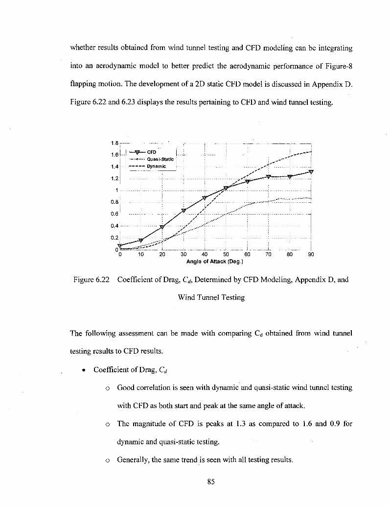
whether results obtained from wind tunnel testing and CFD modeling can be integrating
into an aerodynamic model to better predict the aerodynamic performance of Figure-8
flapping motion. The development of a 2D static CFD model is discussed in Appendix D.
Figure 6.22 and 6.23 displays the results pertaining to CFD and wind tunnel testing.
30 40 50 60 Angle of Attack (Deg.)
90
Figure 6.22 Coefficient of Drag, Cd, Determined by CFD Modeling, Appendix D, and
Wind Tunnel Testing
The following assessment can be made with comparing C<j obtained from wind tunnel
testing results to CFD results.
• Coefficient of Drag, Q
o Good correlation is seen with dynamic and quasi-static wind tunnel testing
with CFD as both start and peak at the same angle of attack.
o The magnitude of CFD is peaks at 1.3 as compared to 1.6 and 0.9 for
dynamic and quasi-static testing.
o Generally, the same trend is seen with all testing results.
85

1.2
1
0.8
0.6
0.4
0.2
-0.2 0 10 20 30 40 50 60 70 80 90
Angle of Attack (Deg.)
Figure 6.23 Coefficient of Lift, C/, Determined by CFD Modeling, Appendix D, and Wind Tunnel Testing
The following assessment can be made with comparing Q obtained from wind tunnel
testing results to CFD results.
• Coefficient of Lift, Q
o From all testing, C/, is initially zero and increases until the stall angle,
o A stall angle of 30° is indicated by CFD, 40° by quasi-static testing, and
45° by dynamic testing. The steady increase in stall angles with testing
type exhibits that air flow detachment at the upper surface steadily
increases by increasing the rate of change in angle of attack.
o The lift is higher in CFD testing as compared to wind tunnel testing. The
use of an infinite wing in CFD provides ideal results which cannot be
reproduced in wind tunnel testing because of airflow around or above the
wing tip of a finite wing.
86
—O—-CFD
--.»•••• Quasi-Static
- - - - - Dynamic
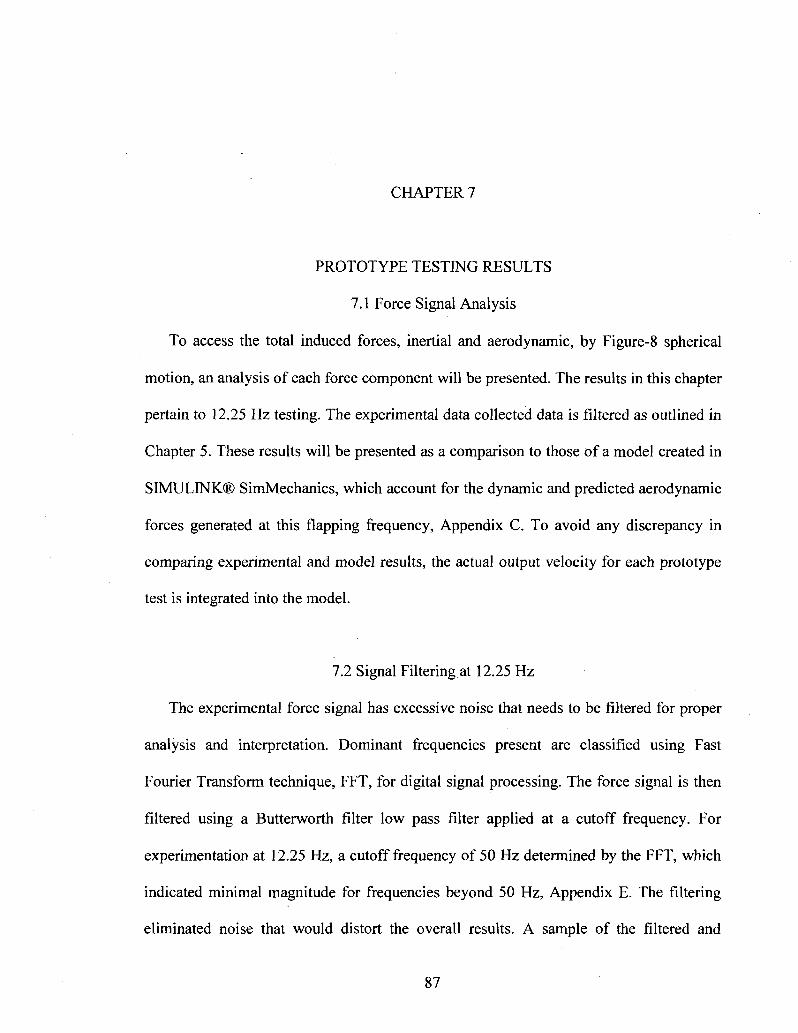
CHAPTER 7
PROTOTYPE TESTING RESULTS
7.1 Force Signal Analysis
To access the total induced forces, inertial and aerodynamic, by Figure-8 spherical
motion, an analysis of each force component will be presented. The results in this chapter
pertain to 12.25 Hz testing. The experimental data collected data is filtered as outlined in
Chapter 5. These results will be presented as a comparison to those of a model created in
SIMULINK® SimMechanics, which account for the dynamic and predicted aerodynamic
forces generated at this flapping frequency, Appendix C. To avoid any discrepancy in
comparing experimental and model results, the actual output velocity for each prototype
test is integrated into the model.
7.2 Signal Filtering at 12.25 Hz
The experimental force signal has excessive noise that needs to be filtered for proper
analysis and interpretation. Dominant frequencies present are classified using Fast
Fourier Transform technique, FFT, for digital signal processing. The force signal is then
filtered using a Butterworth filter low pass filter applied at a cutoff frequency. For
experimentation at 12.25 Hz, a cutoff frequency of 50 Hz determined by the FFT, which
indicated minimal magnitude for frequencies beyond 50 Hz, Appendix E. The filtering
eliminated noise that would distort the overall results. A sample of the filtered and
87

unfiltered force signal for the chord-wise direction, Fx, and the normal direction, Fy, is
shown in Figures 7.1 and 7.2 respectively. Following the signal filtering process, each
force component is compared to that generated by a model for Figure-8 spherical motion
flapping. The main components of interest are the chord-wise force, Fx, and normal force,
Fy, which have both inertial and aerodynamic components present.
1.2 1.25 1.3 Time (s)
Figure 7.1 Unfiltered and Filtered Force Signal for Chord-wise Force, Fx, at 12.25 Hz
88
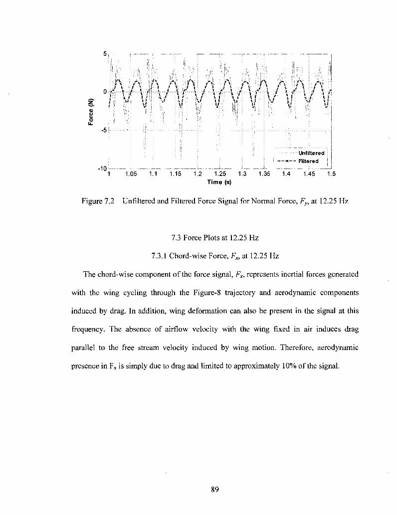
I
m.
-5h
-10
J.* i r • M l V J: . »
Kf M-; • i » •: : Jf :
A : •> v Jlf.'. .
V!
v > --t-y.-» I
A i/ni
y: i r \ i u ! i
\ f
!A V •
--f-T! * J » i ;
1.05 1.1 1.15 1.2 1.25 Time (s)
1.3 „ . . j
1.35
Unfiltered — - a - - Filtered
1.4 1.45 1.5
Figure 7.2 Unfiltered and Filtered Force Signal for Normal Force, Fy, at 12.25 Hz
7.3 Force Plots at 12.25 Hz
7.3.1 Chord-wise Force, F*, at 12.25 Hz
The chord-wise component of the force signal, Fx, represents inertial forces generated
with the wing cycling through the Figure-8 trajectory and aerodynamic components
induced by drag. In addition, wing deformation can also be present in the signal at this
frequency. The absence of airflow velocity with the wing fixed in air induces drag
parallel to the free stream velocity induced by wing motion. Therefore, aerodynamic
presence in Fx is simply due to drag and limited to approximately 10% of the signal.
89

The following analysis can be made from Figure 7.3 which shows a comparison of Fx for
experiment and model.
• Experimental Signal shows higher force magnitude. The higher force magnitude
could be a result of wing deformation. Although the balsa wood wing is fairly
rigid, bending and torsional affects can be present.
• Filtering of the experimental signal may not have completely mitigated the affect
of frequencies that do not correspond to wing testing. However, a lower filtering
frequency cutoff would also create a flattened signal that may eliminate the some
of the aerodynamic and inertial forces.
• As the wing cycles to and from 0° angle of attack where it crosses zero, a
deviation from the model and experiment is noticed. A sharper transition is seen
in the experimental signal as compared the model. This may indicate an incorrect
predication of the aerodynamic force near minimal angle of attack in the model.
90

7.3.2 Normal Force, Fy, at 12.25 Hz
Similar to the chord-wise force, the normal force, Fy, is an essential component of the
for signal that indicates inertial forces and the aerodynamic performance of this motion as
well. The inertial load dominates the signal and limits the aerodynamics to approximately
10%. Deformation is a contributing factor in this force component as a deviation in the
Figure-8 trajectory, widened trajectory along with reference to the symmetry axis along
the stroke plane, can create higher forces unlike the model. The absence of air flow
induces aerodynamic lift present in the normal force signal as the lift force is
perpendicular free stream velocity induced by wing. Figure 7.4 shows the resulting force
signal of both the experimental prototype and model.
: : : • : : : — Theoretical
: : : ; : : : - - - - -— Experimental _3 I L i i i i _ J ii::::^z3zi;zr:::rzzrczzzzzr_
1 1.05 1.1 1.15 1.2 1.25 1.3 1.35 1.4 1.45 1.5
Time (s)
Figure 7.4 Normal Force, Fy, at 12.25 Hz
The following analysis can be made from Figure 7.4 which shows a comparison of Fy for
experiment and model.
91

• Similar to the chord-wise force a deviation between both signals is seen as the
force peaks in the negative y-direction. The higher magnitude during the initial
upstroke can be a result of deformation in the Figure-8 trajectory. Factors
contributing to deformation may include higher testing frequency, wing
flexibility, and any joint looseness particular in the output and coupler hinge joint.
• The higher magnitude along the in the negative y-direction may also indicate the
greater angular acceleration required to drive the mechanism during up-stroking
motion. Little power and angular acceleration is required to transition from 0 -
90° angle of attack; however, the angular acceleration required once the wing has
reached 90° angle of attack may have resulted in the higher force magnitude in
the experimental signal.
e The predicted lift production accounted for in the model may have a limited
contribution as compared to the experimental results.
• Similar to the chord-wise force, the filtering frequency cutoff may have not
completed eliminated noise from the overall signal.
• Overall, aside from the minor difference between the experimental and model
normal force, Fy, indicates matching signals
7.3.3 Span-wise Force, Fz, and the other Force Components
Span-wise force, Fz, induced by Figure-8 spherical motion is generated purely due to
dynamics. The force represents centrifugal effects created with the wing in motion. With
the wing fixed in air, no airflow, aerodynamic forces are not present in the span-wise
force, Fz, as no association with the lift and drag forces can be made. However, the onset
of airflow may present aerodynamic contribution to this force component. Figure 7.5
92

shows the span-wise force, Fz, at 12.25 Hz. As shown, although both results of the model
and experimentation oscillate about an offset value, a much larger force is present during
experimentation. The deviation in Fz is present due to any looseness or movement in the
joints that induces a force in the span-wise during experimentation that cannot be
reproduced in the model. On occasion, collected data for prototype that have been used
extensively, has shown major force contributions in Fz force component further
explaining the reason why it does not match with results of the model. A factor of noise
that is present in all force components may also be indicated by experimental Fz.
Nevertheless, this force component is given little significance as it does not affect the
aerodynamic performance Figure-8 spherical motion flapping. In addition to Figure 7.5,
the remaining force signal components for this testing are shown in the subsequent
Figures. Overall, good correlation is seen in force magnitude, moments, moment
magnitude with any divergence a reciprocal of the difference in the experimental and
model span-wise force, Fz, and slight differences in Fx and Fy.
93

!
1.4 1.5 1.6 Time (s)
Figure 7.5 Span-wise Force, Fz, at 12.25 Hz
Time (s)
Figure 7.6 Force Magnitude of Chord-wise, Fx, and Normal Force, Fy, at 12.25 Hz
94

Figure 7.7 Force Magnitude, F, at 12.25 Hz
Figure 7.8 Moment, Mx, at 12.25 Hz
95

1.4 1.5 1.6 Time (s)
Figure 7.9 Moment, My, at 12.25 Hz
Time (s)
Figure 7.10 Moment, Mz, at 12.25 Hz
96
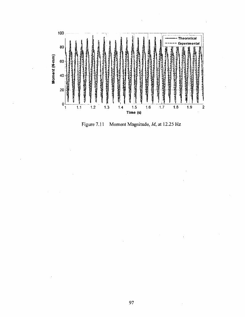
1.1 1.3 1.4 1.5 1.6 Time (s)
Figure 7.11 Moment Magnitude, M, at 12.25 Hz
97
CHAPTER 8
CONCLUSIONS
Figure-8 spherical motion accurately outlines a wing pattern commonly seen in nature
particularly in hovering birds and insects. The integration of such a wing motion offers
promising flight capabilities with potential application to future FWMAV design. The
Figure-8 wing motion was achieved using a spherical four-bar mechanism which outlined
the desired trajectory by attaching the wing to the coupler point. With this mechanism
concept, a prototype was fabricated for testing at varying frequencies of 2.5 - 12.25 Hz to
determine the induced forces by this motion pattern. The acquired force signal was
compared to results of a model to determine the accuracy of both.
8.1 Spherical Four-Bar Mechanism Assessment
Flapping motion as seen in nature is generated by the shoulder joints of many birds
and insects making them capable of creating various wing motions. In this research, a
spherical four-bar mechanism that can mimic the function of a shoulder is successfully
created. A spherical four-bar mechanism was synthesized to create Figure-8 spherical
motion with two planes of symmetry. The synthesized spherical four bar mechanism can
accomplish the desired wing trajectory with precise angular dimension assignment to
each link. The mechanism provided a simple solution to reproducing this complex motion
98

exhibited in nature. The potential benefits of using a spherical four-bar mechanism for
UAV design are outlined.
• The spherical four-bar mechanism can generate various wing trajectories with
manipulation of the link angular dimensions. A distorted or asymmetrical Figure-
8 is attainable to more precisely model in accordance with hummingbird flight.
The various coupler-curves created with assignment of different angular
dimensions gives leeway in manipulation of the mechanism.
• Ability of this mechanism to be used in various class sizes for UAV integration.
The coupler-curve generated is not dependent on the size of the greater sphere the
mechanism occupies; therefore, the size of the overall sphere can be enlarged or
designed for micro application with meticulous manufacturing practices. The only
requirement is that for symmetrical Figure-8 trajectory, for which conditions
specified in Chapter 3 must be satisfied.
8.2 Design and Motion Verification
The conceptual spherical four-bar mechanism was designed and fabricated such that a
wing could be attached to the coupler point. The wing attachment to the mechanism
would ensure feasibility of the design and verify the motion pattern. The fabricated
prototype was tested at various frequencies to determine accurate motion trajectory and
acquire force signals induced by this motion. From the prototype testing conducted, the
motion pattern was verified using still imagery and motion tracking. The motion pattern
resembled the desired wing motion desired and indicated that a spherical four-bar
99

mechanism could be used to generate motion about a shoulder joint as seen in nature.
Advantages of the prototype fabricated included the following.
• Links were designed to have minimal mass. The design of each link ensured the
mass is likely to be limited regardless of the material use. This will minimize
power requirements to drive this mechanism. In this case, the purpose was to
prove concept of the mechanism and its applications; therefore, aluminum was
used.
• Flat surfaces were incorporated into the design of the links for easy connection
and no interference between links. Additionally, space allocation between each
link and permanent hinge joints created with rivets, brass sleeves, and Teflon
rings ensured longevity with limited friction.
• A base was used in place of an input link to enable prototype testing. The base
was attached to an aluminum rod to collect force signals and conduct motion
verification experiments.
• A light weight balsa wood wing was used for prototype testing. The balsa wing
had a limited mass of 3.2 grams further reducing the load on the drive motor. The
minimal mass of the wing also reduced inertial force contribution in the acquired
force signal.
• The minimal mass enabled testing speeds of up to 12.25 Hz. Considering the
conceptual nature of this research, the speeds reached provided valuable insight
on the forces produced by this motion.
100
8.3 Potential Flight Characteristics of Figure-8 Motion
Any practical application is meaningless without a grasp of the potential flight
capability of the designed flapping motion pattern. The aerodynamic performance is
dependent primarily on the lift and drag forces associated with the motion and the
location along the chord length where they are present, Cp. Wind tunnel testing provided
significant information on the lift and drag variation at quasi-static and dynamic change
of angle of attack. The results obtained can be incorporated into a model to better predict
the aerodynamic forces induced by this motion. Furthermore, results were compared to
CFD data that ensured proper analysis of the wind tunnel testing results. The results
indicated a reasonable correlation between wind tunnel testing results with any difference
created by the unknown effect of vortices encountered in the wind tunnel unverifiable by
CFD. Overall, both methods provided a clear indication of how airflow around the wing
behaves when cycling through its Figure-8 spherical motion pattern.
8.4 Prototype Testing Evaluation
Force signal analysis of the extensive experimentation conducted on the fabricated
prototype at various frequencies provided the forces induced by Figure-8 spherical
flapping motion. The results of each test were compared to that of a model and at each
testing frequency showed good correlation. Any deviation in the force signal comparisons
may be a result of factors that are explained in Chapter 7. The good correlation between
both model and experimental prototype also accomplishes a validation of the model
through prototype testing experimentation. Nevertheless, this testing technique can serve
as a verification method to create a more accurate model.
101
8.5 Future Work
Integrating a spherical four-bar mechanism in FWMAV design requires additional
techniques to create a more applicable design and prototype. An appropriate design that
encompasses two wings, more advanced manufacturing process for a more feasible
prototype, and sufficient power production for sustainable flight are primary design
objectives that need to be addressed.
Design of a mechanism that uses two spherical four-bar mechanisms to drive two
wings is essential component that needs to be accomplished prior to FWMAV
application. An ideal design would incorporate both mechanisms using some sort of
shoulder connection and be capable of being driven by a single motor. The use of a single
motor would limit the overall mass of such a prototype and more net lift can be
generated. Limiting mass must also be accomplished by lighter links. The use of material
is vital is minimizing the mass and power requirement. These design enhancements
increase the prospective of more efficient use of aerodynamic forces for more a probable
flight and hover. Mass reduction of the links and wing can be accomplished with the use
of composite materials. The minimal power requirement will establish more practical
designs. Additionally, the minimal mass of the wing can yield enhanced experimentation
by allowing the extraction of aerodynamic forces from acquired load cell data quantifying
the actual aerodynamic forces.
Other work that would institute a perfected design includes developing a 3D dynamic
CFD model, a full dynamic model based on a double wing FWMAV prototype, and
generate control algorithms that would accomplish basic flight tasks. A 3D CFD model
102

would precisely predict the aerodynamic characteristics of Figure-8 spherical flapping
motion. A full dynamic model would help determine the forces generated with the
inclusion of two wings, the results of which could be compared to an actual double wing
prototype. Lastly, a controller design to allow hovering, maneuverability, and feasibility
with respect to nature and application purposes will perfect this design.
103
REFERENCES
[1] Ellington, C , "The Aerodynamics of Hovering Insect Flight. 1. The Quasi-Steady Analysis," Philosophical Transactions of the Royal Society of London. Series B, Biological Sciences, Vol. 305, No. 1122, pp. 1-15, 1984.
[2] Shyy, W., Berg, M., and Ljungqvist, D., "Flapping and flexible wings for biological and micro air vehicles," Progress in Aerospace Sciences, Vol. 35, pp.455-505, 1999.
[3] Ellington, C, "The novel aerodynamics of insect flight: applications to micro-air vehicles," The Journal of Experimental Biology, Vol. 202, pp. 3439-3448, 1999.
[4] Zibikowski, R., Knowles, K., Pedersen, C , and Galinski, C , "Some aeromechanical aspects of insect-like flapping wings in hover," Proc. Institute of Mechanical Engineers Vol. 218 Part G: J. Aerospace Engineering, pp. 389-398, 2004.
[5] Zibikowski, R., Galinski, C , and Pedersen, C , "Four-Bar Linkage Mechanism for Insectlike Flapping Wings in Hover: Concept and an Outline of Its Realization," Journal of Mechanical Design. Vol. 127, pp 817-824, 2005.
[6] Galinski, C. and Zibikowski, R., "Insect-like flapping wing mechanism based on a double spherical Scotch yoke," J. R. Soc. Interface, No. 2, pp. 223-235, 2005.
[7] Banala, S. K. and Agrawal, S. K., "Design and optimization of a mechanism for out-of-plane insect winglike motion with twist," Journal of Mechanical Design. Vol. 127, pp 841-844. 2005.
[8] Mcintosh, S. H., Agrawal S. K., Khan, Z. A., "Design of a mechanism for biaxial rotation of a wing for a hovering vehicle," IEEE/ASME Transactions on Mechatronics. Vol. 11, pp. 145-153. 2006.
[9] Madangopal, R., Khan, Z. A., and Agrawal, S. K., "Energetics-based design of small flapping-wing micro air vehicles," IEEE/ASME Transactions on Mechatronics, Vol. 11, pp. 433-438. 2006.
[10] Conn., A., Burgess, S., Hyde, R., and Ling, C , "From Natural Flyers to the Mechanical Realization of a Flapping Wing Micro Air Vehicle," Proceedings of the 2006 IEEE International Conference on Robotics and Biomimetics, pp. 439-444, 2006.
104

[11] Conn., A., Burgess, S., and Ling, C , "Design of a parallel crank-rocker flapping mechanism for insect-inspired micro air vehicles," Proc. IMechE Vol. 221, Part C: J. Mechanical Engineering Science, pp. 1211-1222, 2007.
[12] Khan, Z. A., and Agrawal, S. K., "Design and Optimization of a Biologically Inspired Flapping for Flapping Wing Micro Air Vehicles," IEEE Conference on Robotics and Automation, pp. 373-378, 2007.
[13] Dickinson, M. H., and Lehmann, F-O., Sane, S.P., "Wing rotation and the aerodynamic basis of insect flight," Science, Vol.284, pp. 1954-1960, 1999.
[14] Sane, S. P., and Dickinson, M. H., "The aerodynamic effects of wing rotation and a revised quasi-steady model of flapping flight," Journal of Experimental Biology, Vol. 205, pp. 1087-1096, 2002.
[15] Singh, B., Ramasamy, M., Chopra I., and Leishman, J.G., "Insect-based flapping wings for micro hovering air vehicles: Experimental investigations," American Helicopters Society International Specialists Meeting on Unmanned Rotorcraft, 2004.
[16] Maybury, W. and Lehmann, F., "The fluid dynamic of flight control by kinematic phase lag variation between two robotic insect wings," The Journal of Experimental Biology, Vol. 207, pp. 4707-4726, 2004.
[17] Khan, Z. A., and Agrawal, S.K., "Force and moment characterization of flapping wings for micro air vehicle applications," American Control Conference, pp. 1515-1520,2005.
[18] Khan, Z. A., and Agrawal, S. K., "Modeling and simulation of flapping wing micro air vehicles," ASME International Design Engineering Technical Conferences and Computers and Information in Engineering, pp. 1-9, 2005.
[19] Lehmann, F. and Pick, S., "The aerodynamic benefit of wing-wing interaction depends on the stroke trajectory in flapping insects," The Journal of Experimental Biology, Vol. 210, pp. 1362-1377,2007.
[20] O., and Angeles, J., "Performance evaluation of path-generating planar, spherical and spatial four-bar linkages," Mechanism and Machine Theory, Vol. 23, pp. 257-268, 1988.
[21] Lu, D., and Hwang, W., "Spherical four-bar linkages with symmetrical coupler curves," Mechanism and Machine Theory, Vol. 31, pp. 1-10, 1996.
[22] Ruth, D., and McCarthy, J., "The design of spherical 4R linkages for four specified orientations," Mechanism and Machine Theory, Vol. 34, pp. 677-692, 1999.
105

McCarthy, J., and Bodduluri, R., "Avoiding singular configurations in finite position synthesis of spherical 4R linkages," Mechanism and Machine Theory, Vol. 35, pp. 451-462,2000.
Alizade, R., and Kilit, O., "Analytical synthesis of function generating spherical four-bar mechanism for the five precision points," Mechanism and Machine Theory, Vol. 40, pp. 863-878, 2005.
Hwang, W., and Chen, K., "Triangular nomograms for symmetrical spherical non-Grashof double-rockers generating symmetrical coupler curves," Mechanism and Machine Theory, Vol. 42, pp. 871-888, 2007.
Duffy, J., "Analysis of mechanisms and robot manipulators," Wiley, New York, 1980.
McCarthy, J., "Geometric Design of Linkages," Springer, Berlin, 2000.
Erdman, A. G., and Sandor, G. N., "Mechanism design analysis and synthesis," Prentice Hall, New Jersey, 1997.
Shigley, J. E., "Kinematic analysis of mechanisms," McGraw Hill, New York, 1969.
"CRC Standard Mathematical Tables, 26th Edition," CRC Press, Boca Raton, 2000.
Ketchel, J., and Larochelle, P., "Computer-aided manufacturing of spherical mechanisms," Mechanism and Machine Theory, Vol. 42, pp. 131-146, 2007.
http://www.ati-ia.com/products/n7ft_models.aspx?id=Nano 17
http://www.faulhaber-group.com/uploadpk/EN_2057B_MIN.pdf
http://www.micromo.com/nll2782/i364354.html
Larijani, R. F., and DeLaurier, J. D., "A nonlinear aeroelastic model for the study of flapping wing flight," AIAA Progress in Aeronautics and Astronautics, Vol.195, chap 18, pp. 399-428, 2001.
106

APPENDIX A
EQUATIONS OF MOTION FOR FIGURE-8 SPHERICAL MOTION
Duffy [26] presented the equations for a general spherical four-bar mechanism by
splitting the quadrilateral into two spherical triangles. As mentioned earlier, Figure-8
motion of a coupler point can be achieved by creating a spherical four bar-mechanism
with the following angular dimensions:
(X41 = a i2 = CI23 = otp = 9 0 °
eP=-90°
In this case, the generalized equations of can be reduced to:
• sin(«34) sin(#4) ± y 1 - sin2(a34 )cos2 (<94) 0.=2 tan"
cos feJ (A.1)
The above equation produces two values of 0i, each for one of the closures of the
mechanism. Each value of 0i can be used to calculate the corresponding values of 02 and
03-
# 2 = 2 tan" sin(or34) sin(#4) cos(#,) -f- cos(a34) sin(#,)
sin(ar34)cos(#4)+l (A.2)
<93 = 2 tan -1 cos(#4) sin(#,)
cos(ar34) sin(6>4) sin(#,) + sin(or34) cos(<9,) +1 (A.3)
107
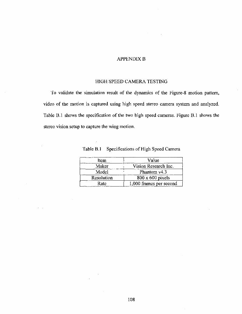
APPENDIX B
HIGH SPEED CAMERA TESTING
To validate the simulation result of the dynamics of the Figure-8 motion pattern,
video of the motion is captured using high speed stereo camera system and analyzed.
Table B.l shows the specification of the two high speed cameras. Figure B.l shows the
stereo vision setup to capture the wing motion.
Table B. 1 Specifications of High Speed Camera
Item Maker Model
Resolution Rate
Value Vision Research Inc.
Phantom v4.3 800 x 600 pixels
1,000 frames per second
108

Figure B.l High Speed Camera Stereo Vision Setup
The stereo camera calibration is performed to measure the intrinsic and extrinsic
parameters of stereo camera. A total of seven left and right images of a planar
checkerboard with 10 mm black and white squares were used. Figure B.2 is a snapshot of
both the left and right calibration images. Table B.2 and Table B.3 shows the intrinsic
and extrinsic parameters of left and right camera that indicate the position of right camera
with respect to left camera. Actual designed distance between centers of lens is 120 mm
and calibrated baseline distance is a reasonable value of 119.423 mm with 0.245 mm
error. Forty-four light reflecting marks are placed on the wing. The marks are placed 10
mm apart as shown in Figure B.3. Figure B.4 shows the left and right image of stereo
camera system which captures the Figure-8 wing motion.
109

t f l « f *
«w
J • , / * * ? ' % ^ *. -** F 4 »
B "i * #% ? * i "• * ' *
: \ , * t t . - , * i
f ' » , * ; \ <•* r *• • ' V X A A /
*>
* * "8
' - '̂ V **«^>
S^^
,
-is w > .*<
' { > I4", -f" • „ l .
' i ! *•** fl
£ X ) l * *, V A v / X / S ^ ^ *.
A J V , , jt ^ a
J"* -% v
< V *
(A)
^ ' * % * 1 * ^ ' ^ ^ * ^ y ^ *
(B)
Figure B.2 Stereo calibration images (A) left camera image (B) right camera image
110

Table B.2 Stereo Camera Intrinsic Parameters
Parameters Left Camera Focal Length
Left Camera Principal point Left Camera Distortion
Right Camera Focal Length Right Camera Principal point
Right Camera Distortion
Value [1173.634, 1172.916]+/-[3.870, 3.6301 pixels
[373.847, 321.243]+/-[6.183, 6.205] pixels [=0.324, 0.1317, =0.000, =0.005, 0.000]
[1165.211, 1170.397]+/=[3.790, 3.206] pixels [377.151, 322.301]+/-[6.218, 7.204] pixels
[-0.332, =0.025, 0.001, -0.001,0.000]
Table B.3 Stereo Camera Extrinsic Parameters
Parameters Rotation Vector
Translation vector
Value [0.011, 0.002, 0.002]+/-[0.007, 0.007, 0.001] rad.
[-119.423,-0.699, 4.119]+/-[0.245, 0.151, 1.562] mm
jv
... " ' I Q*
*
.
!' VO!
6 '
' ,
Q, a"
3" f
- ^ U
* *
i "
;& 'p>- 6 (
&%#%•<!« fs./t<J <V,s
•
-
*° 9. a 3,iO 6
• „ ' ,
*
o
-
,
o ' " w
1
9 0
• .
•f* \
,
•"
,
^
, .
Figure B.3 Wing with Designated Points for Motion Tracking
111

*
'< e eP
>• \ , '" -« « ^
^t .̂' * i V*," "
3
* * . J . *
• - » *» ' * * J >.< " *0 s °"
""»'„< *«', '* 'i> il / ' * * f *'* » * . * * , .
°'l- '
1 ' * • *
(A)
4 ., *
t
• ; ^ ^ -"»,4» **
« * • * .
w, Ji« \
fii • 1
J fj> «̂ *v
(B)
Figure B.4 Stereo wing motion images. (A) Left camera image, (B) right camera image
112

APPENDIX C
AERODYNAMIC MODELING
Defining the aerodynamics associated with Figure-8 flapping spherical motion
required a thorough understanding of how the movement of air over the surface of the
wing would act. As compared to fixed wing flight which has fixed angle of attack and
uses propulsion to generate movement across the air, flapping motion exhibited by
hummingbirds and insects, produce flight with its flapping wings. Therefore, rapid
changes in direction, velocity induced by the wings, angle of attack, and phase of the
motion are all distinct aerodynamic features that accomplish flight. In determining the
aerodynamic model, [35] allows us to comprehend certain characteristics to account for
in flapping wing flight. With modifications made for spherical motion, theory discussed
in [35] is employed into to our model to determine the aerodynamics produced by this
motion.
C.l Defining Induced Free-stream Velocity
The free stream velocity generated by Figure-8 flapping motion is defined as the
velocity induced over on the wing acting tangent to the wing trajectory as shown in
Figure C.l. This definition holds for any flapping motion as long as the system's position
is held constant or fixed at a single location. Therefore, the induced velocity for any point
on the subdivided section on the wing, P„ is defined in Equation C.l.
113
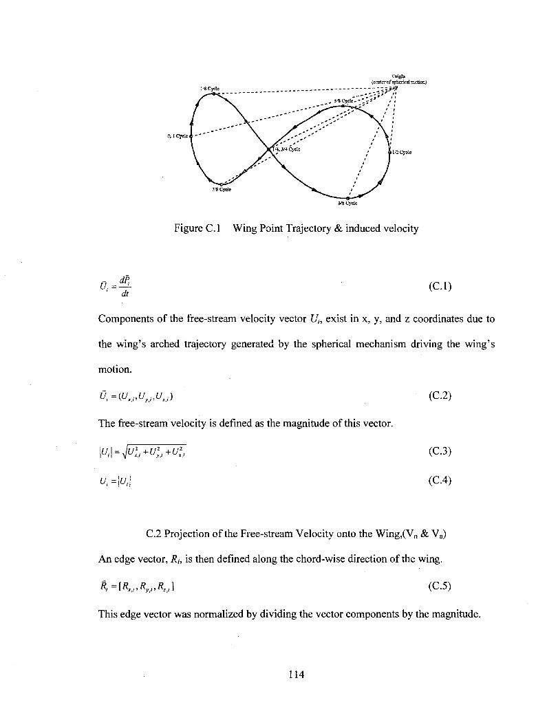
(cancrof3pha5calTn&tioc) 1-* Cycle
CUCyel.
hi Cycle
7,* Cycle
3/8 Cycle
Figure C.l Wing Point Trajectory & induced velocity
' dt (C.l)
Components of the free-stream velocity vector Uh exist in x, y, and z coordinates due to
the wing's arched trajectory generated by the spherical mechanism driving the wing's
motion.
O^iu^u^u,,)
The free-stream velocity is defined as the magnitude of this vector.
M=>K+£/,2,+^,
u,=\u,\
(C.2)
(C.3)
(C.4)
C.2 Projection of the Free-stream Velocity onto the Wing,(Vn & Va)
An edge vector, Rh is then defined along the chord-wise direction of the wing.
Ri -[Rx,i>Ry,i>R:,i] (C.5)
This edge vector was normalized by dividing the vector components by the magnitude.
114

*«=M (C7)
The free-stream velocity, Uh was then projected into the surface of the wing by taking the
dot-product of the normalized edge vector, RNii, along the wing and the free-stream
velocity vector, Uh as shown in Figure C.2.
Kj = V, • K = (Ki •U*,,) + (*,, • Uy,) + ( ^ • V,.,) (C8)
Figure C.2 Induced wing velocity projection
This dot-product projection of the free-stream velocity was used to determine the velocity
acting normal to the wing, V„:i.
Vni =\Ui\sin(a') (C.9)
The work presented here is based on the assumption that the wing acts as a perfectly
rigid body. This assumption was made as a simplification to the experimental model. The
wing used on this study is based on scaling the forewing of a dragonfly as presented in
115

[16], has a slightly tapered thickness. The irregular shape associated with the wing profile
used in the model makes it particularly difficult to integrate the aerodynamic forces that
act upon it. Therefore, it is approximated by / rectangular sections of uniform thicknesses.
To eliminate the wing's shape complexity, the wing span area was subdivided into six
equal span length areas. In order to approximately represent the wing's actual area at the
locally subdivided span length, L„ the chord length, c„ of these rectangular sections were
chosen. As shown in Figure C.3, this approximation holds that the subdivided span area
of each subdivided rectangle equals that of the actual models span area over the locally
subdivided span length.
Outter Edge
Inner Edge
'- | CIMPS
CI,<P* i a C-.P.
Cl«P, I CI/4P2
CP» CPJ
CP. « CP,
L _""^ - J - - 4
I
- 0 . 1 6 7 L -
C„«P. Origin
® CP2
CP,
Figure C.3 Approximate Wing-Sub Area Divisions
The centers of these rectangles, used as the point of measurement for the induced velocity
on the local wing subdivided area, were chosen to be at the mid-chord length and the
mid-span length of each subdivided rectangular section. With the wings coordinate
system being defined at the inner edge of the wing and center to the mounting point.
c/>(x,jO = | y ' f (CIO)
116
In a similar fashion, the quarter chord point of these rectangles, used as the point of
application of the aerodynamic resultant force on the local wing subdivided area, were
chosen to be at the quarter-chord length from the leading edge and the mid-span length of
each subdivided rectangle.
Cu<P,(x,y) = {^) (CM)
It is assumed that the resultant of the aerodynamic forces acts at the quarter-chord length
of each sub-divisional area. This assumption was based on the center of pressure, Cp,
being approximately located at the quarter chord location as understood in thin airfoil
theory.
C.3 Derivation of Aerodynamic Forces
For the model, partial leading-edge suction, vortex wake effects, and post-stall
behavior were accounted for along the wing's sectional profile. The resultant forces
obtained from this model were then applied to the quarter-chord point of each subdivided
area and measured at the same point of reference as the experimental model. To begin the
study of the aerodynamic forces, a division was made to separate the forces occurring
during attached and detached flow. Figure C.4 shows all the aerodynamics forces with
respect to the wing cross-section.
117

"^z*. **l*
- ^ T.
Mid-Chord
Figure C.4 Wing Section Aerodynamics forces and motion variables
C.4 Attached Flow
The aerodynamic resultant force acting at the quarter chord point is given by,
HAJ = ̂ + ^ (C12)
where RnJ is the resultant force normal to the wing profile and Raj is the resultant force
in the chord-wise direction of the wing. The resultant force normal to the wing profile is
given by,
where Ncj is the circulatory normal force and Naj is the apparent-mass normal force. The
resultant force in the chord-wise direction is given by,
KJ=T„-D„ (C.14)
where D/j is the viscous drag force due to skin friction and Tsj is the leading-edge
suction force. The circulatory normal force is given by,
Ncj=\f*J,vaM (C.15)
where, p is the density of air at standard pressure,
Uj is the free-stream velocity,
118

Vaj is the free-stream velocity component in the chord-wise direction of the wing,
Cn is the normal force coefficient,
c, is the chord length, and
/, is the span length of the particular subdivided rectangle.
The apparent-mass effect normal force is given by,
NaJ=±p*c,2U,d'l, (C.16)
where a ' i s the change in the angle of attack with respect to the change in time. The
viscous drag force is given by
Df^Ca^-c,l, (C.17)
where Ca is the force coefficient in the chord-wise direction of the wing profile. The
leading-edge suction force is given by
TlJ=n,2x(a')2?^clIl (CAS)
where i/s is the leading-edge suction efficiency which is assumed to be 0.5.
C.5 Detached (Stalled) Flow
The wing profile transitions into a stall condition when the angle of attack increases
between the free stream velocity and the wing's sectional profile, thus causing the flow to
detach from the upper surface of the wing creating turbulent vortices. This flow
detachment will progress until it has reached the leading edge of the wing at which point
stall occurs. The aerodynamic resultant force is given by,
(^,)SMW= («,,,)-, +(^,)«* (C19)
119

where (Rn,i)staii is the resultant force normal to the wing profile and (Ra,i)stau is the
resultant force in the chord-wise direction of the wing. The resultant force normal to the
wing profile is given by,
(K,Xall=(KA,n+(Ka,Xan ( C 2 0 )
where (Nc,i)staii is the circulatory normal force during stall conditions and (Na,i)staii is the
apparent-mass normal force during stall conditions. The resultant force in the chord-wise
direction is given by,
{K,Xa,l={TS,Xa,l-Wf,Xall (C.21)
where {Dc^stau is the viscous drag force due to skin friction and (TStj)stau is the leading-
edge suction force. The circulatory normal force is given by,
K , L = ( C . ) ^ < , ' , (C.22)
where Vn>j is the free-stream velocity in normal to the wing profile. The apparent-mass
effect normal force is given by,
(".^-^j^W.*')', (C23)
The viscous drag force is given by,
DLi=Ca^f-Cil, (C.24)
The leading-edge suction force is given by,
T^rj^ia'f^c,!, (C.25)
120

C.6 Dynamic Stall Condition
The angle of the attack at which full flow separation occurs over the upper surface of
the wing changes as the angle of attack is changed dynamically. Dynamic stall occurs at
higher angles of attack due to delayed flow separation and the suction force created by
the opposed turbulent vortices at the leading and trailing edge. In [35], this is modeled as
the angular difference between static and effective (dynamic) stall as,
( « - ) ^ - ( « - ) . = A a = ^ (C.26)
where £ is determined experimentally and is dependent on the local Mach number.
(C.27) Acr = 0.51
°W=M
c • \ a 2U
121

APPENDIX D
CFD MODELING
A CFD model to determine the aerodynamic performance of the wing as it reaches
high angle of attack is developed as part of another subtask for this research. A 2D static
model is developed for a thin plate with equivalent dimensions to that of the wing used
for prototype testing. The wing is subjected to wind and pressure conditions similar to
that of wind tunnel testing. To vary the angle of attack, the direction of the velocity
vector towards the horizontally aligned wing cross sectional geometry is incrementally
changed with results analyzed. Initially the velocity vector is parallel to the wing and then
increased at 10° increments until 90° angle of attack is reached. Using CFD modeling,
the coefficient of lift, Q, and drag, Cd, are calculated. The results of CFD modeling are
compared to wind tunnel testing results to ensure validity of the modeling and provide
insight of the flight characteristics with an infinite wing. As mentioned in Chapter 6,
although the results vary in magnitude, a similar trend indicates acceptable correlation
between CFD modeling and wind tunnel testing. These results also provide information
about the aerodynamic performance of the wing at high angle of attack.
122

APPENDIX E
PROTOTYPE TESTING PLOTS
Prototype testing is conducted at various testing speeds to interpret the forces
produced by Figure-8 wing motion. Additionally, a comparison of results is made with
the force model created in SIMULINK® SimMechanics. The experimental testing of the
prototype is conducted at 2.5 Hz, 5 Hz, 7.5 Hz, 10 Hz, and 12.25 Hz. With a discussion
of the results for 12.25 Hz presented in Chapter 7, the remaining testing results will be
discussed in this section.
To determine the filtering frequency, the FFT of chord-wise force, Fx, and normal
force, Fy, is examined. For the data plotted in Chapter 7 for 12.25 Hz flapping frequency,
the cutoff frequency was determined to be 50 Hz. From the FFT of the Fx, Figure E.l,
maximum amplitude of 1.4 is at 12.21 Hz, which indicates the testing frequency of the
prototype. Frequencies beyond 12.21 Hz have lower amplitudes and at 49 Hz, lower
order amplitude of 0.2 is reached. The FFT of Fy, Figure E.2, shows maximum amplitude
of 1.3 at 21.41 Hz. The double cycle in the y direction during the Figure-8 motion
corresponds to the double testing frequency displayed for Fy. Similarly, frequencies
beyond the testing frequency begin to diminish and amplitude of 0.59 is reached at 49
Hz. Therefore, the cutoff frequency for 12.25 Hz prototype testing is determined to be 50
Hz.
123

1.5
U-a> •a | Q. E <
0.5
10 10 Frequency (Hz)
Figure E.l Unfiltered Data FFT for Chord-wise Force, Fx, at 12.25 Hz
a> •a
E <
1.4
1.2
0.8
0.6
0.4
0.2
-•••••]"v|-j j[ |r|| {•••{•i"nij{i "tTijiiitr--:"i rf-nfif
10 10" 10' Frequency (Hz)
10' 10"
Figure E.2 Unfiltered Data FFT for Normal Force, Fy, at 12.25 Hz
124

For filtering at 2.5 Hz testing, an analysis of the FFT for both Fx and Fy is used to
locate the cutoff filtering frequency. From the FFT of Fx, Figure E.3, we notice maximum
amplitude for the testing frequency and lower amplitude thereafter. Twice the testing
frequency is indicated for Fy, Figure E.4, because of the double cycle and frequencies
beyond 20 Hz indicate the noise in the signal. Therefore, for prototype testing results at
2.5 Hz flapping, 20 Hz is determined to be the cutoff frequency. This FFT analysis
methodology is applied to all testing frequencies to determine the most adequate cutoff
frequency.
0.07
0.06
0.05
a> •5 0.04
| 0.03 <
0.02
0.01
10 10 10 Frequency (Hz)
10' 10"
Figure E.3 Unfiltered Data FFT for Chord-wise Force, Fx, at 2.5 Hz
125

0.06
0.05
0.04
I 0.03 a. E <
0.02
0.01
10 10 10 Frequency (Hz)
10 10"
Figure E.4 Unfiltered Data FFT for Normal Force, Fy, at 2.5 Hz
The plots below, Figures E.5-E.13, show the comparison of the experimental and
model results for testing at 2.5 flapping frequency. Good correlation is seen in chord-wise
force, Fx, and the normal force, Fy. To eliminate noise, the experimental force signal was
filtered at 20 Hz as determined by the FFT of Fx and Fy. Difference in experimental
results could account factors discussed in Chapter 7. For the span-wise force, Fz, the
difference in signal could be explained by any looseness in joints creates force along this
direction and cannot be reflected in the model. Overall good correlation is seen with
model and experimental results.
126
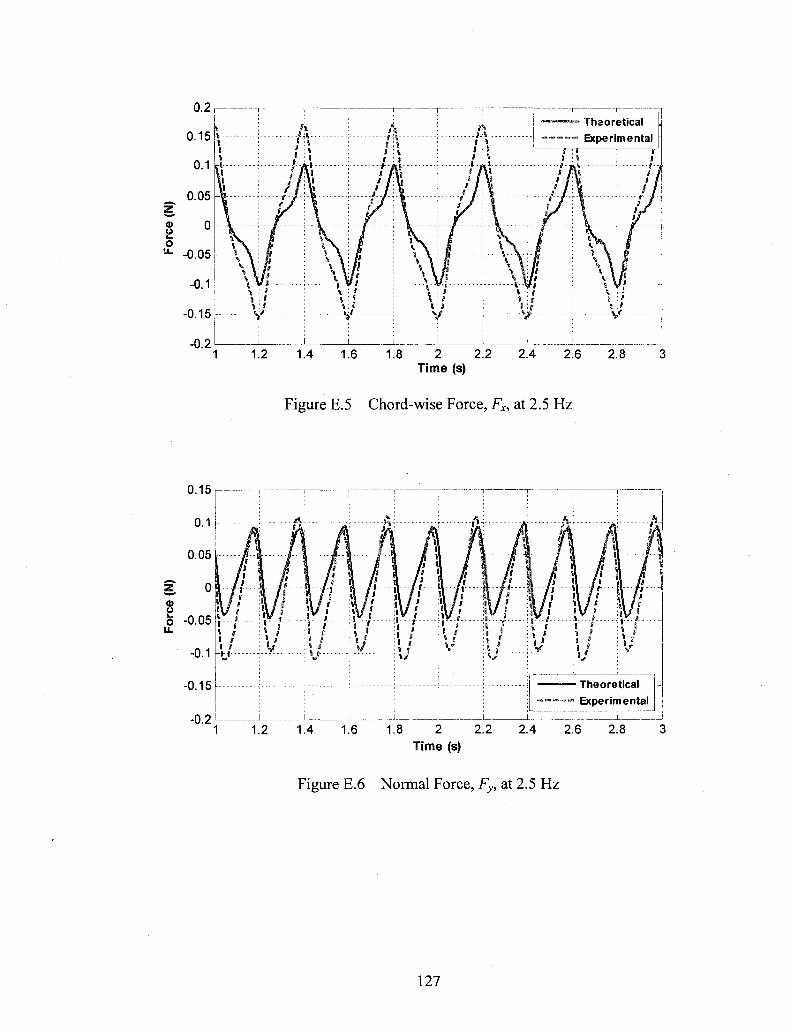
Figure E.5 Chord-wise Force, Fx, at 2.5 Hz
-0.05
-0.15
1.2 1.6 1.8 2 2.2 Time (s)
Figure E.6 Normal Force, Fy, at 2.5 Hz
127

0.1
0.08
0.06
S. 0.04
0.02
) A • • i - - j - - f i f * i f %
A /
M
1.2
: i
!'. : - * •
• * / * f i *
7T
» *
A y
IV-
A J *
j :»
4 /
i : I > r r - - i - * - - r - - - J
: \ I • • • - I
,i -
• Theoretical Experimental
1.4 1.6 1.8 2 Time (s)
2.2 2.4 2.6 2.8
Figure E.7 Span-wise Force, Fz, at 2.5 Hz
0.15
0.05
Figure E.8 Force Magnitude of Chord-wise, Fx, and Normal Force, Fy, at 2.5 Hz
128
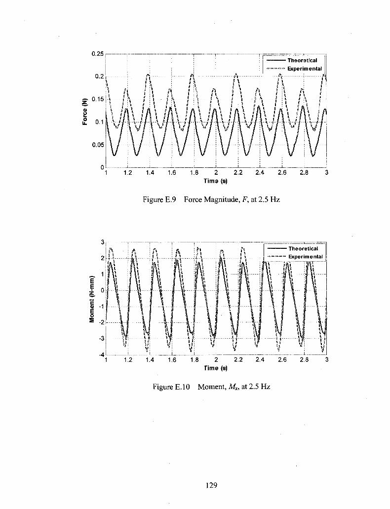
0.25
Figure E.9 Force Magnitude, F, at 2.5 Hz
Figure E. 10 Moment, Mx, at 2.5 Hz
129

Time (s)
Figure E. 11 Moment, My, at 2.5 Hz
Figure E. 12 Moment, Mz, at 2.5 Hz
130
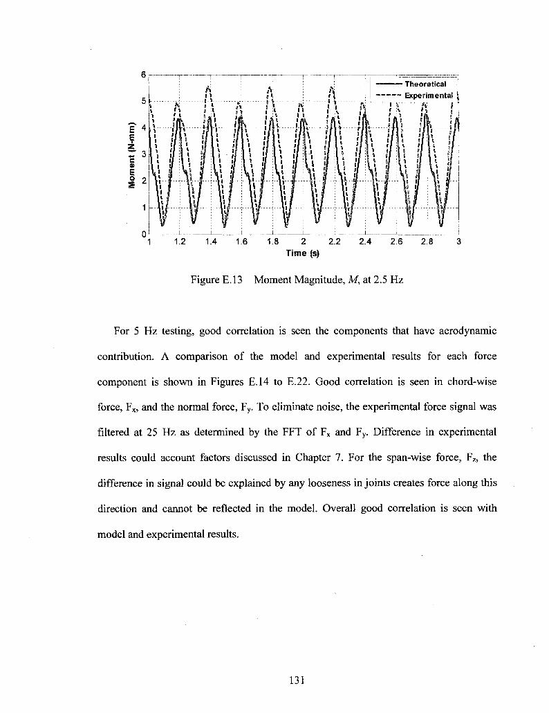
Time (s)
Figure E. 13 Moment Magnitude, M, at 2.5 Hz
For 5 Hz testing, good correlation is seen the components that have aerodynamic
contribution. A comparison of the model and experimental results for each force
component is shown in Figures E.14 to E.22. Good correlation is seen in chord-wise
force, Fx, and the normal force, Fy. To eliminate noise, the experimental force signal was
filtered at 25 Hz as determined by the FFT of Fx and Fy. Difference in experimental
results could account factors discussed in Chapter 7. For the span-wise force, Fz, the
difference in signal could be explained by any looseness in joints creates force along this
direction and cannot be reflected in the model. Overall good correlation is seen with
model and experimental results.
131
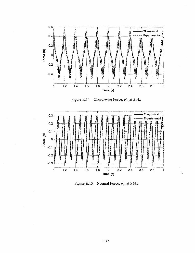
" - "1 "
0.2
A 4 IJ! J:i..
' Theoretical
Experimental
'"ll""
u ----ft--
w V
L
! f - | -l j : [J : %'
i i
-if-u
u *?
1.2 1.4 1.6 1.8 2 2.2 Time (s)
2.4 2.6 2.8
Figure E.14 Chord-wise Force, Fx, at 5 Hz
1.8 2 2.2 2.4 Time (s)
Figure E. 15 Normal Force, Fy, at 5 Hz
132
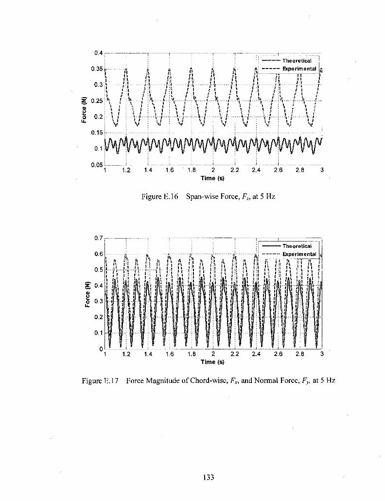
0.4 r
0.15
- -«
Lh f r v ' " " i "
0.05
•ni-I : i I ;« II ' 1
• • - » • -
P
' ' i
fit ' ; ' f i
t
t I - •
— — Theoretical .____ Experimental j |
a. *
% 1 I
;l
r -\ • -
• t I
# f f i i
8 . f V
J! ' : I • - « • ; + -
s i
J - - -J- -
I #
l ; l "Y";t"'
/ :»
I V"J""
Figure E.16 Span-wise Force, Fz, at 5 Hz
' Theoretical
1.8 2 2.2 Time (s)
Figure E.17 Force Magnitude of Chord-wise, Fx, and Normal Force, Fy, at 5
133

1.8 2 2.2 Time (s)
Figure E.l 8 Force Magnitude, F, at 5 Hz
Figure E. 19 Moment, Mx, at 5 Hz
134
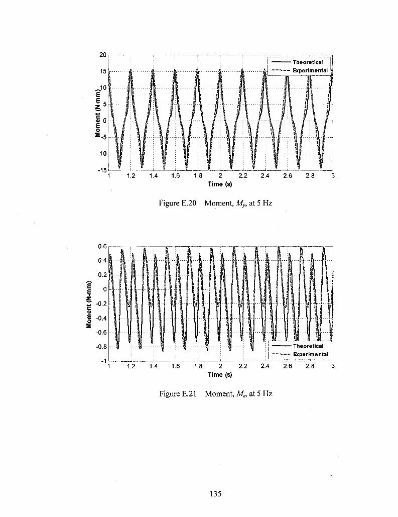
Theoretical _____ Experimental
1.8 2 2.2 Time (s)
Figure E.20 Moment, My, at 5 Hz
1.2 1.8 2 2.2 Time (s)
Figure E.21 Moment, Mz, at 5 Hz
135

Similarly, good correlation in results between model and experimental data is seen at
7.5 Hz flapping frequency. A comparison of the model and experimental results for each
force component is shown in Figures E.23 to E.31. Good correlation is seen in chord-
wise force, Fx, and the normal force, Fy. To eliminate noise, the experimental force signal
was filtered at 35 Hz as determined by the FFT of Fx and Fy. Difference in experimental
results could account factors discussed in Chapter 7. For the span-wise force, Fz, the
difference in signal could be explained by any looseness in joints creates force along this
direction and cannot be reflected in the model. Overall good correlation is seen with
model and experimental results.
136

Figure E.23 Chord-wise Force, Fx, at 7.5 Hz
1.4 1.5 Time (s)
Figure E.24 Normal Force, Fy, at 7.5 Hz
137

£ 0.4
1.4 1.5 1.6 Time (s)
Figure E.25 Span-wise Force, F2, at 7.5 Hz
Figure E.26 Force Magnitude of Chord-wise, Fx, and Normal Force, F>» at 7.5 Hz
138

1.4 1.5 1.6 Time (s)
Figure E.27 Force Magnitude, F, at 7.5 Hz
g" 10
1 1.1 1.2 1.4 1.5 1.6 Time (s)
Figure E.28 Moment, Mx, at 7.5 Hz
139
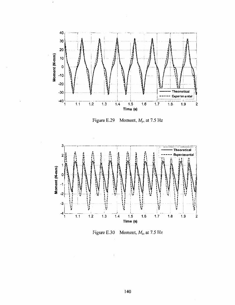
Figure E.29 Moment, My, at 7.5 Hz
' Theoretical Experimental
Time (s)
Figure E.30 Moment, Mz, at 7.5 Hz
140

4 0 f " ™ ™ - - " T ™ " " ! ™ " ™ T ' " " " " " T ™ ™ ' H " " ^
For 10 Hz testing, good correlation is seen the components that have aerodynamic
contribution. A comparison of the model and experimental results for each force
component is shown in Figures E.32 to E.40. Good correlation is seen in chord-wise
force, Fx, and the normal force, Fy. To eliminate noise, the experimental force signal was
filtered at 40 Hz as determined by the FFT of Fx and Fy. Difference in experimental
results could account factors discussed in Chapter 7. For the span-wise force, Fz, the
difference in signal could be explained by any looseness in joints creates force along this
direction and cannot be reflected in the model. Overall good correlation is seen with
model and experimental results.
141

1.4 1.5 1.6 Time (s)
Figure E.32 Chord-wise Force, Fx, at 10 Hz
Figure E.33 Normal Force, Fy, at 10 Hz
142
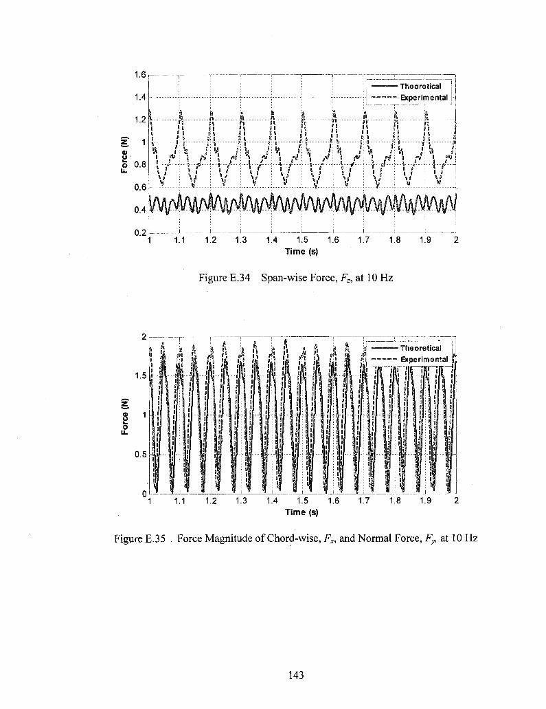
1.6
1.4
1.2
z 1 <D U
o 0.8 u.
0.6
0.4
0.2
J - J l — -." J» f'1
»: *, D . * *
' i I - - : - - - » •
: *
B - f l -SS
it 11 (:~f "
• - J l -
J;* -n-v
HI i: i i; •
- « r i -
• ' / ' . •
4.
J
-I--V-
V V
i T" U
4 1
'A a
- ->i - • u si i: l
' Theoretical Experimental
at • • » » • •
11
i
* ft "l\ ft -Jr -a r.-i
l
«: T." i:
I
V
1.1 1.2 1.3 1.4 1.5 1.6 Time (s)
1.7 1.8 1.9
Figure E.34 Span-wise Force, Fz, at 10 Hz
1.1 1.4 1.5 1.6 Time (s)
Figure E.35 Force Magnitude of Chord-wise, Fx, and Normal Force, Fy, at 10 Hz
143

2.5 L i i, ij Theoretical | j j K h ,1 , $ / . I " " — Experimental ,
i ?i :' 1.1 : : i i i !:• Ji »:i i\ i: • » J : 1 *® ';» i t ": . I i: i «
u. 1
1.1 1.2 1.3 1.4 1.5 1.6 Time (s)
1.7 1.8 1.9
Figure E.36 Force Magnitude, F, at 10 Hz
Figure E.37 Moment, M» at 10 Hz
144

-60
' Theoretical Experimental
WiV ;
w 1 \ 1 w 1
1.1 1.2 1.3 1.4 1.5 1.6 Time (s)
1.7 1.8 1.9
Figure E.38 Moment, My, at 10 Hz
1.4 1.5 1.6 Time (s)
Figure E.39 Moment, Mz, at 10 Hz
145

Figure E.40 Moment Magnitude, M, at 10 Hz
146

VITA
Graduate College University of Nevada, Las Vegas
Zohaib Parvaiz Rehmat
Home Address: 5622 Sage Pines Drive Las Vegas, NV 89118
Degrees: Bachelor of Science, Mechanical Engineering Technology Vaughn College of Aeronautics and Technology
Publications: Design of "Figure-8" Spherical Motion Flapping Wing for Miniature UAV
(submitted) Flight Characteristics of Flapping Wing Miniature Air Vehicles with "Figure-8"
Spherical Motion (submitted)
Thesis Title: Design of a "Figure - 8" Spherical Motion Flapping Wing for Miniature UAV's
Thesis Examination Committee: Co-Chairperson, Mohamed B. Trabia, Ph.D. Co-Chairperson, Woosoon Yim, Ph.D. Committee Member, Georg Mauer, Ph.D. Committee Member, Brendan J. O'Toole, Ph.D. Graduate Faculty Representative, Edward Neumann, Ph.D.
147