design manual for engineering analysis of...
TRANSCRIPT

ARIZONA
DEPARTMENT OF WATER RESOURCES
DESIGN MANUAL FOR
ENGINEERING ANALYSIS
OF
FLUVIAL SYSTEMS
1985

DESIGN MANUAL FOR ENGINEERING ANALYSIS
OF FLUVIAL SYSTEMS
Prepared for
Arizona Department of Water Resources99 East Virginia AvenuePhoenix, Arizona 85004
By
Simons, Li & Associates, Inc.
120 West Broadway, Suite 170P.O. Box 2712
Tucson, Arizona 85702
3555 Stanford RoadP.O. Box 1816
Fort Collins, CO 80522
Project Number AZ-DWR-05RDF162, 166, 232/R522
March 1985

ACKNOWLEDGEMENTS
This manual was prepared for the State of Arizona, Department of Water
Resources, by Simons, Li & Associates, Inc. (SLA). The contract was under thesupervision of Mr. Robert L. Ward, P.E., Chief of the Flood Control Section,
Department of Water Resources. Under his guidance and direction, a truly use-ful, practical design manual was developed. The Project Manager at SLA was
Mr. Michael E. Zeller, P.E., and the primary author was Dr. James D. Schall,
P.E. Input data and calculations for the comprehensive design example pre-sented in Chapter VII were provided by Ms. Pat Deschamps, P.E., Project
Engineer, Department of Water Resources. Technical review was provided by Dr.Ruh-Ming Li, P.E. The Department of Water Resources also wishes to
acknowledge the financial contribution and review comments provided by the
Flood Control District of Maricopa County. The District's participation in
this project was greatly appreciated.

CONDITIONS OF USE
This manual was developed by Simons, Li & Associates, Inc. under contract
to the State of Arizona, Department of Water Resources. The use of thismanual by any individual or group entity is with the express understandingthat Simons, Li & Associates, Inc. and the State of Arizona make no warran-ties, express or implied, concerning the accuracy, completeness, reliability,
usability, or suitability for any particular purpose of the information con-tained herein. Furthermore, neither Simons, Li & Associates, Inc. nor theState of Arizona shall be under any liability whatsoever to any such indivi-dual or group entity by any reason of use made thereof.

TABLE OF CONTENTS
Acknowledgments iiConditions of Use i i iList of Figures v i i iList of Tables xiDefinition of Symbols x i i i
I. INTRODUCTION 1.1
II. GENERAL DESIGN CONSIDERATIONS
2.1 Channel and Watershed Response 2.12.2 Sand-Bed Channels 2.32.3 Cobble-Bed Channels 2.42.4 General Solution Approach 2.5
2.4.1 Three-Level Analysis 2.52.4.2 Level I - Qualitative Geomorphic Analysis 2.52.4.3 Level II - Quantitative Geomorphic and Basic
Engineering Analysis 2.62.4.4 Level III - Quantitative Analysis Using
Mathematical Models 2.6
2.5 Data Requirements 2.7
2.5.1 General 2.72.5.2 Level I Data Requirements 2.72.5.3 Level II Data Requirements 2.82.5.4 Level III Data Requirements 2.122.5.5 Data Generation Concepts 2.12
III. HYDROLOGIC ANALYSIS
3.1 Relation ofHydrology toOther Analyses 3.13.2 Establishing Return Period Discharges and Durations 3.2
3.2.1 General 3.23.2.2 Rational Method 3.43.2.3 SCS TR-55 Methods 3.63.2.4 USGS Flood-Frequency Analysis 3.63.2.5 Other Regionalized Methods 3.73.2.6 Channel Geometry Techniques 3.7
3.3 Development of Flood Hydrographs 3.8
3.3.1 General 3.83.3.2 Characterization of Design Storm 3.8
I V

TABLE OF CONTENTS (continued)
Page
3.3.3 Determination of Runoff Volume 3.113.3.4 Hydrograph Development 3.13
3.4 Selection of Design Event for Fluvial Systems Analysis .... 3.133.5 Discretizing Flood Hydrographs 3.17
IV. HYDRAULIC ANALYSIS OF ALLUVIAL CHANNELS
4.1 General 4.14.2 Resistance to Flow 4.1
4.2.1 Common Resistance Parameters and TheirRelationships 4.1
4.2.2 Resistance to Flow in Fine-Grained AlluvialChannels 4.4
4.2.3 Resistance to Flow in Cobble/Boulder-BedAlluvial Channels 4.8
4.3 Boundary Shear Stress Calculations 4.154.4 Normal Depth Calculations 4.18
4.4.1 Definition 4.184.4.2 Normal Depth Calculation for Trapezoidal Channels . . . 4.214.4.3 Normal Depth Calculation for Natural Channels 4.22
4.5 Water-Surface Profiles 4.224.6 Additional Effects on Flow Depth in Alluvial Channels .... 4.23
4.6.1 Importance 4.234.6.2 Antidune and Dune Height . 4.244.6.3 Superelevation 4.244.6.4 Debris Accumulation 4.294.6.5 Total Freeboard Requirement 4.29
4.7 Examples , 4.31
4.7.1 Analysis of Resistance to Flow in Sand-Bed Channels . . 4.314.7.2 Analysis of Flow in Rough Channels 4.34
V. SEDIMENT TRANSPORT ANALYSIS
5.1 General Concepts 5.1
5.1.1 Basic Sediment Transport Theory 5.15.1.2 Basic Terminology 5.3

TABLE OF CONTENTS (continued)
Page
5.2 Level I Analys is 5.4
5.2.1 Plan Form Characterist ics 5.45.2 .2 Lane Relat ion and Other Geomorphic Relat ionships . . . 5.115.2.3 Aerial Photograph Interpretation 5.165 .2 .4 Bed- and Bank-Material Analysis 5.205.2 .5 Land-Use Changes 5.225.2.6 Flood History and Rainfall-Runoff Relations 5.24
5.3 Level II Analys is 5.25
5.3.1 Watershed Sediment Yield 5.255.3.2 Detailed Analysis of Bed and Bank Material 5.315.3 .3 Profile Analysis 5.385.3 .4 Incipient Motion Analysis 5.425.3.5 Armoring Potential 5.455.3.6 Sediment Transport Capacity 5.505 .3 .7 Equil ibrium Slope 5.735.3.8 Sediment Continuity Analysis 5.825.3.9 Quanti f icat ion of Vertical and Horizontal Channel
Response 5.875.3.10 Local Scour Concepts 5.925.3.11 Contraction Scour 5.1025.3.12 Bend Scour 5.1055.3.13 Evaluat ion of Low-Flow Channel Incisements 5.1105.3.14 Evaluat ion of Gravel Mining Impacts 5.1115.3.15 Cumulative Channel Adjustment 5.116
5.4 Level III Analysis 5.119
5.4.1 General 5.1195.4.2 Application of Level III Analysis 5.119
VI. CHANNEL DESIGN CRITERIA
6.1 General = . 6.16.2 Bank/Levee Height 6.16.3 Bank/Levee Toedown 6.26.4 Lateral Migration" 6.26.5 Grade-Control Structures 6.56.6 Common Bank Protection Methods 6.6
VII. COMPREHENSIVE DESIGN EXAMPLE
7.1 Project Description 7.17.2 Level I 7.17.3 Level II 7.8
VI

TABLE OF CONTENTS (continued)
Page
7.3.1 Levee Embankment Height . 7.87.3.2 Levee Embankment Stabi l izat ion 7.11
7.3.2.1 Eros ion of Embankment Material 7.117.3.2.2 Toe-Down Requirement For Stabi l iza t ion System . . . . 7.12
7.3.2.2.1 Armor Potential 7.127.3.2.2.2 Long-Term Aggradation/Degradation 7.147.3.2.2.3 Low Flow Incisement 7.227.3.2.2.4 Local Scour 7.237.3.2.2.5 General Scour 7.257.3.2.2.6 Sand Wave Troughs 7.32
7.3.3 Lateral Migration 7.33
7.4 Summary and Conclusions 7.37
VIII. REFERENCES 8.1
APPENDIX A - PACIFIC SOUTHWEST INTER-AGENCY COMMITTEE (PSIAC) METHODFOR PREDICTING WATERSHED SOIL LOSS
APPENDIX B - MODIFIED UNIVERSAL SOIL LOSS EQUATION (MUSLE) FORPREDICTING WATERSHED SOIL LOSS

LIST OF FIGURES
Figure 1.1
Figure 1.2
Figure 1.3
Figure 1.4
Figure 2.1
Figure 2.2
Figure 3.1
Figure 3.2
Figure 3.3
Figure 4.1
Figure 4.2
Figure 4.3
Figure 4.4
Figure 4.5
Figure 4.6
Figure 4.7
Figure 4.8a
Figure 4.8b
Figure 5.1
Figure 5.2
Pjig_e
October 1983 flood, Pantano Wash, Tucson, Arizona 1.2
October 1983 flood, Rillito River, Tucson, Arizona .... 1.3
October 1983 flood, Santa Cruz River, Tucson, Arizona . . . 1.4
October 1983 flood, R i l l i t o River, Tucson, Arizona 1.5
Watershed-river system 2.2
Definition sketch illustrating typical measured sedimentdischarges vs. water discharge relation 2.10
Typical sediment yield frequency curve 3.15
Definition sketch of the hydrograph discretizationprocess 3.18
Hydrograph discretization 3.19
Forms of bed roughness in sand-bed channels 4.9
Relation of bed form to stream power and medianfall diameter of bed sediment 4.11
Variation of boundary shear stress in a trapezoidalcross section 4.16
Maximum unit tractive force versus aspect ratio (b/d) . . . 4.17
Effect of bend on boundary shear stress 4.19
Definition sketch of the energy and hydraulic grade linesin open-channel flow 4.20
Definition sketch of antidune height 4.25
Definition sketch of superelevation in a channel bend . . . 4.26
Definition sketch of superelevation and flow separationconditions in a short radius bend 4.26
Definition of sediment load components 5.2
River channel patterns 5.5
vm

LIST OF FIGURES (continued)
Page
Figure 5.3 Classification of river channels 5.8
Figure 5.4 Schematic of the Lane relationship for qualitativeanalysis 5.12
Figure 5.5 Slope-discharge relations 5.14
Figure 5.6 Channel pattern versus slope and sinuosity 5.15
Figure 5.7 Example illustrating qualitative information derived fromtime sequence analysis of aerial photographs 5.21
Figure 5.8 Annual rainfall for Santa Margarita watershed 5.26
Figure 5.9 Maximum annual mean daily discharge for Santa MargaritaRiver 5.27
Figure 5.10 Annual runoff-rainfall ratio for Santa Margaritawatershed 5.28
Figure 5.11a Selected particle size gradations 5.39
Figure 5.lib Representative gradation curve 5.40
Figure 5.12 Shields' relation for beginning of motion 5.43
Figure 5.13 Frequency of motion for various particle sizes 5.46
Figure 5.14 Armored bed of Salt River upstream of Gilbert Roadnear Mesa, Arizona, and excavation through armorlayer of the Salt River near Mesa Arizona 5.48
Figure 5.15 Relationship of discharge of sands to mean velocity for sixmedian sizes of bed sands, four depths of flow, and a watertemperature of 60°F 5.59
Figure 5.16 Colby's correction curves for temperature, fine sediment,and median particle size 5.60
Figure 5.17 Bed material gradation curve for example using ColbyMethod 5.64
Figure 5.18 Log - log plot of uncorrected sediment discharge (qs^)vs. hydraulic depth (Yu) 5.65
Figure 5.19 Relationship between equilibrium slope and channelbed controls 5.78
IX

LIST OF FIGURES (continued)
Page
Figure 5.20 Existing and Equilibrium Slope Profiles for Example Problem 5.83
Figure 5.21 Temporal change of scour hole depth during a storm 5.93
Figure 5.22 Common pier shapes 5.95
Figure 5.23 Scour increase factor KaL, for piers not aligned withflow 5.98
Figure 5.24 Definition sketch of embankment length "a" 5.100
Figure 5.25 Illustration of terminology for bend scour calculations . . 5.107
Figure 5.26 Relative time for filling a gravel pit and reachingequilibrium for a low and high flow event 5.113
Figure 5.27. Critical time for erosion of a flood-plain gravel pit . . . 5.115
Figure 5.28. Definition sketch of the temporal changes at theupstream edge of a gravel pit 5.117
Figure 6.1. Calculated risk diagram 6.3
Figure 7.1. Project plan view, Pinto Creek at Sportsman's Haven .... 7.2
Figure 7.2. Time sequence analysis of historical aerial photographs . . 7.4
Figure 7.3. Comparison of historical bed profiles 7.6
Figure 7.4. Block diagram of Level II analysis 7.9
Figure 7.5. Average gradation curve, Pinto Creek at Sportsman's Haven . 7.15
Figure 7.6. Cross-section geometry for upstream sedimentsupply section , 7.18
Figure 7.7. Plan view of levee alignment analyzed in localscour evaluation 7.24
Figure 7.8. Discretized 100-year flood hydrograph 7.27
Figure 7.9 Sediment transport rating curve - Reach 2, Pinto Creekat Sportsman's Haven 7.28

LIST OF TABLES
Page
Table 2.1
Table 2.2
Table 3.1
Table 3.2
Table 3.3
Table 4.1
Table 4.2
Table 4.3
Table 5.1
Table 5.2
Table 5.3
Table 5 4
Table 5.5
Table 5 6a
Table 5 6b
Table 5.7
Table 5 8
Table 5.9
Table 5 10
Table 5.11
Partial Listing of Data Requirements for a Level I
Partial Listing of Data Requirements for a Level II
USGS Offices with WATSTORE Information
USGS Offices with NAWDEX Information
Water and Sediment Discharge Data for HydrographDiscretization Example . .
Values of Manning's Coefficient n for Design of Channelswith Fine to Medium Sand Beds
Superelevation Formula Coefficients
Agencies with Information on Aerial Photographs
Recommended Size Range, Analysis Concentration,and Quantity of Sediment for Commonly Used Methods
Minimum Recommended Sample Weights for Sieve Analysis . . .
Sediment Transport Calculation Procedures
Results of Regression Analysis 0 001 < S0 < 0.01
Results of Regression Analysis 0 01 < S0 < 0 04
Range of Parameters Examined for Power Relationships ....
Rpnmpfn'r Mpsn Pal ml at innc; fnr Tnlhv Fxflfliolp
Uncorrected Sediment Transport Rate for Colby Example . . .
Total Spriimpnt Transport Ratp for folbv Examole .
Bed Material Discharge Calculations for Colby Method ExampleUsina Sediment Size Fractions
? q
2.11
3.3
3.5
3.20
4.5
4.10
4.28
5.19
5.34
5.35
5.47
5.52
5.55
5.56
5.57
5.68
5.68
5.71
5.72

LIST OF TABLES (continued)
Page
Table 5.12 Short-Term General Scour/Deposition Response 5.88
Table 5.13 Sediment Continuity Results (100-Year Flood) 5.91
Table 5.14 Reduction Factors When Applying Formulas for Square NosePiers to Other Shapes 5.97
Table 7.1 Equilibrium Slope Calculations for Reach 2 7.21
Table 7.2 General Scour Analysis Using Sediment Continuity 100-yearEvent 7.29
Table 7.3 Pinto Creek 100-year Sediment Continuity Analysis 7.31
Table 7.4 Calculation of Antidune Trough Depths 7.34
Table 7.5 Summary of Soil Cement Toe-down Dimensions 7.39
XI 1

DEFINITION OF SYMBOLS
A Area
A Total wetted roughness cross-sectional area
b Bottom width
b Pier width
b Roughness geometry parameter in Bathurst's procedure (19781C Chezy resistance factor
c Sediment concentration (ppm by weight)
d Depth of flow measured normal to direction of flowD Diameter of pipe
D Sediment particle size of the armor layeraD Sediment particle size at incipient motion
D. Percent finer particle size (i.e. 0™, DQO, etc.)f Darcy-Weisbach friction factor
F.B. Freeboard distanceFr Froude number
Fr Pier Froude number
G Gradation coefficient
G Specific gravityg Acceleration of gravity
h Antidune height from crest to troughahf Friction loss
L Lengthn Manning's roughness coefficient
p ProbabilityP Wetted perimeter
P Percent of material coarser than armor sizeL>
q Water discharge per unit width
Q Water discharge
q. Bed-load transport per unit width
q Peak water discharge per unit width
q Bed-material sediment discharge per unit width
R Hydraulic radius
r Radius of curvature
R Pier Reynolds number
xm

S Slope
S Slope of energy gradient
S Slope of channel bed
SgQ Median size of short axis of particle in Bathurst's procedure (1978)
T Top width
t Time of concentration
V Mean velocity
V* Shear velocity
VOL. Water volume from probability weighting111 L«
VOL Water volume from gaging station data
VOL Sediment volume
W Width of f low
X Distance downstream of a channel bend at which secondary f low oecomesnegl igible
Y Depth of f low measured vertically
y Crit ical f low deptn
Y, Hydraulic depth
y Normal deptn
Y,-^ Median size cross-stream axis of particle in Bathurst 's procedure(1978)
z Side slope angle (horizontal:!)
Ay Additional f low depth due to long-term aggradation
Ay, Additional f low depth from debris accumulation
Ay Additional f low deptn from separation in short-radius bends
Ay Superelevation
AZ Depth to formation of armor layeraAZ, Bend scour depth
AZ, Change in bed elevation from long-term degradation
AZ General scour depth
A Z . Low-f low channel incisement depth
AZ Local scour depth/v J
AZ Total vertical adjustment in bed e levat ionL \J U
Y Specific weight of water
Y Specific weight of sedimentp Density
T Critical tractive force
xiv

T Boundary shear stress (tractive force)
a Standard deviation
u Kinematic v iscosity
TT Pi (3.14)
xv

1 • INTRODUCTION
The rigid boundary conditions upon which most flood control studies are
currently based do not acknowledge the potential for river systems to move
both laterally and vertically. Failure to address this problem in the design
and construction of flood control projects, bridges or other structures
located within a flood plain can lead to their premature destruction or obso-
lescence. Recognizing this deficiency in typical design procedures, the
Arizona Department of Water Resources initiated development of this design
manual.
The purpose of this design manual is to present techniques and procedures
that may be used to make a thorough engineering analysis of major fluvial
systems in order that the natural processes associated with such systems can
be accounted for in the design of flood control projects. The importance of
this is vividly illustrated by the photographs in Figures 1.1 to 1.4.
Figures 1.1 (Pantano Wash - Tucson, Arizona) and 1.2 (Rillito River -Tucson, Arizona) illustrate the lateral migration that can occur during a
flood. In particular, the power line poles of Figure 1.1 illustrate the
extent of lateral migration possible during a single flood. Figures 1.3
(Santa Cruz River - Tucson, Arizona) and 1.4 (Rillito River - Tucson, Arizona)
illustrate the potential for both loss of life and property during a single
event. In Figure 1.3, the Cortaro Farms Road bridge was completely destroyed,
and in Figure 1.4 a townhome is on the verge of falling into the river. The
situations illustrated all developed during the October 1983 flooding in
southeastern Arizona. The need for an engineering analysis in order to pre-
dict fluvial system response, and to design adequate mitigating measures that
will prevent or limit the dangers illustrated in Figures 1.1 to 1.4, is self-
evident.Information in this manual addresses the dynamics of watershed and chan-
nel systems considering hydrologic, hydraulic, geomorphic, erosion and sedi-
mentation aspects. The emphasis is placed upon practical implementation of
state-of-the-art technology in identifying, evaluating and designing for thenatural processes associated with major fluvial systems. Depending upon engi-
neering judgment and project economics, the principles discussed herein can
also be applied to the design of small conveyance drainage systems. Only that
information considered absolutely essential to understanding the basic theory
of the application procedures has been presented, while other relevant, but
1.1

Figure 1.1. View from the Speedway Blvd. bridgelooking upstream along the east bankof the Pantano Wash, Tucson, Arizona(Photo date: October,1983).
1.2

<cncO
5-
O ••-
CO
ccCTl
O)
"OJC
S
-+->
03
rs 3
O
Ot/1 4->
E
4J
O
tnS~
(1)~
S
+->O)
s_•r-
O>
c
cus_3en
01 m
-
-C
C
S-
-M
O
Ol
N _n
S- -r- O
O)
S-
4->>
<C
OO
O
O)
Ccr. O
••
TD
I/) O
l•r-
U -M
i-
3
ro-Q
I—
-O
OJ
•> O
3
S-
-!->C
C
U O
<U
>
JCZ
> -i-
D
_•=c D
;—-

C -5 rt>
OJ
•*—""
^£2
> Q
J OJ
-a -
s r+
n
rr -
j.
-st-t
- o
O
Nl
rt
OO
3
(D
CDQ
-O
> co O n t-t-
o cr fD -5
-sG
O
<-t-
OOJ rr
3r+
ro
DJ n
a)
o to
o
-s
t-t-
-S
rt-
c
oj
crN
~S
Q
Jo
rs
33
7T
<
O
—"
rt>
DJ
o-5
C
L
O
1.0
cr -j.
oo
—i
-s
rsoo
c:
-j. xj
-—-
o o.
« t/>
;o ^
O
CD
CD3
to

Figure 1.4. View from the west bank lookingnortheast across the Rillito River,Tucson, Arizona(Photo date: October, 1983).
1.5

non-essential, information has been cited by reference only. This approach
allows the user who might be interested in details to locate the desired
information, while allowing those who are not so interested in details to
efficiently proceed through the design process.
Design manual organization provides a logical sequence of steps to guidethe user from start to finish, both through individual elements of a single
design and the overall integration of many elements of a comprehensive fluvial
system analysis and design effort. Hydro!ogic Analysis (Chapter III) is the
first major analysis after General Design Considerations (Chapter II). After
completing the hydrologic analysis, information required as input for
Hydraulic Analysis of Fluvial Channels (Chapter IV) is available. Similarly,
results of this analysis are required prior to Sediment Transport Analysis
(Chapter V). Chapter V completes the analysis component, providing the base-
line data and knowledge necessary for application of various channel design
techniques discussed in Chapter VI. To illustrate the integration of infor-
mation resulting from each chapter, a comprehensive design example is given in
Chapter VII.
The design manual is targeted for use by practicing engineers in the
water resources field, or other individuals with equivalent knowledge ortraining. Consequently, an understanding of the basic concepts of hydrology
and hydraulics has been assumed. Only that information necessary or essential
to analysis of sediment transport is reviewed and/or provided in Chapters III
and IV, resulting in a brief, highly-specialized treatment of the subject.
Should additional information be required on general concepts, the user is
referred to any hydrology and/or hydraulics textbook.
In contrast, subject material in Chapter V on Sediment Transport Analysis
is presented in more detail. Beginning with Subsection 5.2, each subsection
consists of three elements: DISCUSSION, APPLICATION, and EXAMPLE. The dis-
cussion material briefly describes the usefulness of the methodology and pre-
sents relevant theory and equations. The applications material presents
information necessary to apply the methodology including rules of thumb and
reasonable parameter values. Finally, an example is presented. Typically, it
represents a simplistic case only intended to illustrate key points; however,when practical, these examples are based on case histories.
1.6

11 • GENERAL DESIGN CONSIDERATIONS2.1 Channel and Watershed Response
A generalized definition of the idealized fluvial system is the three-
zone description provided by Schumm (1977). In this description, Zone 1 is
the drainage basin, watershed, or sediment source area; Zone 2 is the transfer
zone; and Zone 3 is the sediment sink, or region of deposition. The three
subdivisions are based on the predominant processes occurring in each, since
sediments are stored, eroded, and transported in all zones. Zone 1 involves
primarily the upper watershed and various tributary watersheds that contribute
to the channel network of Zone 2. Zone 3 concerns primarily the coastal
region, since this is considered the ultimate deposition zone. Consequently,
in the analysis of inland watersheds, such as those of Arizona, Zone 3 is not
of immediate importance and the fluvial system is often redefined as the
interaction of the watershed and the alluvial channel network. Figure 2.1
provides a conceptual drawing of the fluvial system as defined.
Limiting our scope to this definition of the fluvial system still defines
a highly complex system involving the interaction of many natural processes.
These natural processes, often referred to as physical processes, govern the
response of the fluvial system to various inputs and/or disturbances. The two
primary inputs are climatic factors and man's activities. The most importantclimatic factor for erosion/sedimentation analyses is precipitation, in the
form of either rain or snow. Man's activities include water resources devel-
opment, watershed conversion, resource acquisition (energy, sand/gravel,
etc.), development and operation of transportation systems, etc.
The response of the fluvial system to these inputs and/or disturbances is
governed by the relevant physical processes. For example, the physical pro-
cess describing soil detachment from raindrop impact is important in evaluat-
ing system response to precipitation. The physical process of overland flow,
described by the interaction of such factors as slope, roughness, and precipi-
tation excess, defines watershed response by establishing sediment transport
supply available during a given precipitation event. Similarly, within the
channels of the fluvial system, the physical processes describing sedimenttransport capacity establish whether or not the channel will aggrade or
degrade in response to the precipitation-generated water and sediment runoff.
2.1

Upstream Watershed Tributary Watershed
Figure 2.1. Watershed-r iver system.
2.2

Throughout all these events man's activities will modify fluvial systemresponse by influencing the governing physical processes. Perhaps the most
important concept to realize about fluvial systems is that they are dynamic
systems attempting to achieve a state of balance or equilibrium. Conse-
quently, the fluvial system is either adjusting to altered conditions or is ina state of dynamic equilibrium with present conditions. In either case,
natural and man-induced changes can initiate responses that may be propagated
through long periods of time or large areas. This dynamic nature requires
that the analysis of problems (even on a small, localized scale) and develop-
ment of solutions be considered in terms of the entire system. A classicexample illustrating the dynamic nature of the fluvial system is the implemen-
tation of flood control reservoirs or debris basins. These structures can
induce downstream degradation by limiting the delivery of upstream sediments.
The dynamic action-response mechanisms of fluvial systems must be acknowledgedand incorporated into any analysis or design effort, small or large.
2.2 Sand-Bed Channels
The analysis and design of fluvial systems in sandy-soil regions presents
unique problems not encountered with more well-developed soils. In this
context, "sandy" is used in the engineering sense to describe loose, cohesion-less soils. Sandy soils are most predominant in the semi-arid and arid
regions of the country. In comparison, the higher precipitation of a more
humid environment produces vegetation and soils that are well developed and
stabilized. Under these natural conditions, streams carry low suspended sedi-
ment loads reflecting the stability in upland watersheds. Additionally, highprecipitation produces a dilution effect on the sediments that are eroded.
Vegetation and land forms in arid and semi-arid regions reflect the lack
of water. Compared with more humid regions, topography is more abrupt, hill-
slopes are usually steeper and shorter, and soils are thinner with little
organic content. Dryland conveyances are usually incised, intermittent or
ephermeral channels. When the channels do flow, it is usually in response to
small storm cells of limited areal extent producing high-intensity, short-
duration storms. This type of storm creates "flashy" runoff, producing both
excessive erosion in upland watersheds and a pronounced capacity for sediment
transport in the channel system. Due to high drainage density (number of
channels per unit area), water and sediment runoff occurs very efficiently.Peak discharge is high, and time to peak and flow duration are short.
2.3

The combination of large sediment yield, large transport capacity and
"flashy" runoff can cause rapid changes in the configuration of sandy-soil
channels. These changes include lateral migration, scour, degradation and
aggradation, and can cause changes in stream form, bedform, flow resistance
and other geometric and hydraulic characteristics. Designing either a stable
alluvial channel (one without a channel lining) or a stable, lined channelunder such dynamic conditions requires a detailed understanding of sedimenttransport and stream channel response. For example, unlined channels must be
designed to minimize excessive scour, while lined channels must be designed to
prevent deposition of sediments. Channel linings in dryland areas are typi-
cally composed of some type of artificial stabilization due to the difficul-
ties in growing the required type of vegetation. Unlined channels are most
successful when designed under the concept of dynamic equilibrium, whichsimply allows for sediment transport conditions without scour. These topics
and others are presented in detail in the following chapters.
2.3 Cobble-Bed Channels
The erodibility or stability of any channel largely depends on the size
and gradation of particles in the bed. As water flows through a channel
located in a well-graded alluvium (i.e. consisting of clay, silt, sand, gravel
or boulders) smaller particles that are more easily transported are carried
away while the larger particles remain. This process, referred to as
armoring, results in what will be defined as a cobble-bed channel, although
the particles remaining on the bed can be as small as gravels. Compared tothe more uniformly graded sand-bed channel, cobble-bed channels are relativelystable; however, they are still moveable boundary channels that can experience
significant change during floods. Therefore, one of the important factors in
cobble-bed analysis or design is evaluation of the stability of the armor
layer and the maximum discharge it can sustain without being disrupted.
Another category of cobble-bed channels, in addition to those developed
through the armoring process, are the boulder-lined channels of steep moun-
tainous regions. Except in very large floods, these channels are very stable,
with water cascading through sections of rapids connected by pools. This
characteristic of flow and the large size of the roughness elements inhibits
analysis by the more common and familiar techniques applicable to relatively
2.4

flat channels. When appropriate, brief discussions of analysis and design
techniques for these very specialized conditions are presented.
2•4 General Solution Approach
2•^•1 Three-Level Analysis
The recommended solution procedure for sediment transport analysis gener-ally involves three levels of analysis. The levels are defined as (I) quali-
tative, involving geomorphic concepts; (II) quantitative, involving geomorphic
concepts and basic engineering relationships; and (III) quantitative, involv-
ing sophisticated mathematical modeling concepts. A qualitative Level I anal-ysis provides insight into complicated fluvial system response mechanisms.
The general knowledge obtained at this level provides understanding and direc-
tion to the Level II or III quantitative analysis. Additionally, the govern-
ing physical processes are usually identified in the general solutions of
Levels I and II, allowing proper selection (or development) of a model for
Level III that is efficient to use and applicable to the problems being ana-
lyzed. For long-term analysis where data are continually collected and/or
updated, an iterative procedure of refinement becomes an important aspect of
Levels II and III. As the data base becomes more complete and accurate, the
type and level of analysis can become more sophisticated.
The three-level approach has been used extensively in the Southwest, and
has been found to provide the most efficient analysis approach with the great-
est accuracy for a given problem. The risk is minimized, since all results
and conclusions are cross-checked to the other levels of analysis. The
following paragraphs discuss some of the important concepts in each level of
analysis.
2-4-2 L e v e l I - Qualitative GeomorphicAnalysis
The qualitative geomorphic analysis employed in Level I relies strongly
on expertise and practical experience. Geomorphology is the study ofsurficial features of the earth and the physical and chemical processes ofchanging land forms, while fluvial geomorphology is the geomorphology (and
mechanics) of watershed and river systems. Qualitative geomorphic techniques
are primarily based on a well-founded understanding of the physical processes
governing watershed and river response. Therefore, an important first step is
to assemble and review previous work and data applicable to the study area,
2.5

and for key project participants to become familiar with the study area. A
site visit by key personnel ensures identification of important characteris-
tics of the study area. Additionally, being in the study area and contacting
the local interest groups concerned provides excellent insight and perspective
for the study. Site visits are an essential element of a successful study.
After completing the necessary site visits there are a number of
simplified concepts and procedures that contribute to a qualitative analysis.
These include aerial photograph analysis, historical land-use patterns, andrelatively simple relationships describing basic geomorphic concepts. The
Level I analysis is discussed in detail in Section 5.2-
2.4.3 Level II - Quantitative Geomorphic and Basic__E_ngi_n_eering Analysis
In Level I, geomorphic principles are applied to predict watershed andstream response and do not require detailed data, only a general understanding
of the direction of change of the stream conditions. Geomorphic principles
can also be applied to available data to more accurately evaluate watershed or
channel responses. This analysis, when coupled with traditional analysesinvolving basic engineering relationships, allows an initial quantitative eva-
luation of response. Analysis techniques used in Level II involve evaluation
of trends in the historical thalweg elevation, quantitative evaluation of bed
and bank sediments, application of the Shields relation and other geomorphic/
engineering relations, application of sediment transport equations and the
sediment continuity principle, frequency analysis of water and sediment
transport data, etc. Level II analyses can be completed by hand calculator;
however, use of a computer can expedite some calculations. For example, the
analysis of sediment continuity using appropriate sediment transport relations
is also often completed with the aid of computer programs. A detailed
discussion of the Level II analysis is presented in Section 5.3.
2-4.4 Level JII - Quantitative Analysis Using Mathematical Model_s
The Level III analysis is the most accurate method of analysis andinvolves computer application of various physical-process mathematical models.
A mathematical model is simply a quantitative expression of the relevant phys-
ical processes. Various types of mathematical models for sediment routing are
available, depending on the application (watershed or channel analysis) and
the level of analysis necessary. For example, channel models range from
2.6

application of quasi-dynamic models (such as HEC-6 or HEC-2SR) to complicated
dynamic sediment routing methods. In general, available models can be
directly applied, or applied with minor modifications, to meet any project
requirements. Criteria for electing to proceed with a Level III analysis are
presented in Section 5.4.
2.5 Data Requirements
2.5.1 General
The quality and accuracy of any analysis are dependent on the data base
available to the study. The type and number of data necessary depend greatly
upon the sophistication of the analysis techniques (i.e., whether Level I, II,
or III); however, for any analysis the level of effort required to establish
the data base can represent a significant portion of the entire level of
effort. The data base is developed from available data and any data collected
during the project. Below is a brief discussion of the data requirements foreach of the three levels of analysis.
2.5.2 Level I Data Requirements
The data required for a Level I geomorphic type analysis involves infor-
mation on general trends and conditions describing the fluvial system charac-
teristics, rather than specific, quantitative values. Some of the geomorphic
relations used to qualitatively describe system action-response (the Lane
relation or the slope-discharge relation) rely on estimates of dominant slope
and/or discharge; however, due to the nature of the formulas and their
intended applications, these numbers do not need to be accurate, refined
values.Other data required in a geomorphic analysis involve information
describing historical trends or patterns. This information is generally
interpreted on a qualitative basis, relying largely on personal experience and
expertise. A typical example is the analysis of aerial photographs covering
a span of several years. The amount of information extracted depends in parton the years covered. Similarly, insight derived from analysis of the flood
history of a given drainage depends on the length of record available.
2.7

Table 2.1 summarizes some of the major data requirements of a Level I
analysis.
2-5.3 Level II Data Requirements
Level II data requirements involve specific estimates of various parame-ters necessary to apply a range of quantitative geomorphic and basic engi-
neering formulas. The data required might include specific, detailed numeri-
cal information on the watershed geometry (area, slope, length, drainage den-
sity, channel characteristics), sediment produced and delivered by the
watershed (water discharge, sediment discharge, soil types, geology, repre-sentative particle sizes transported, gradation), man's influence (dams, sand
and gravel extraction), and so forth. For many larger watersheds, data on
these processes have been collected by various governmental agencies. The
quality of the data and the length of record often vary so that careful eva-
luation is required to insure the data are useful for the purposes of the
study. For example, most sediment discharge data have been collected onlyduring low-flow periods; however, it is commonly accepted that the majority of
sediment transport occurs during relatively short periods of high flow.Plotting low-flow sediment discharge data against water discharge for a given
watershed generally produces poor results with no apparent trend.
Consequently, data extrapolation or establishment of a descriptive equation
for the watershed would appear impossible. However, if several additional
high-flow data points were available, a distinguishable trend might be
established (see Figure 2.2).
This situation can develop even when data have been collected over many
years if no major storms occurred during the period of record. Therefore, the
available data must be carefully interpreted and used to avoid erroneous
conclusions. Additionally, the available data base is typically much smaller
that that required to conduct the study. Consequently, the necessary addi-
tional data must be established by field measurement or by data generation
techniques. A brief overview of several basic concepts in data generation is
given in Section 2.5.5.Some of the specific data requirements necessary to conduct a Level II
analysis are presented in Table 2.2.
2 0.o

Table 2.1. Partial Listing of Data Requirementsfor a Level I Analysis.
General Channel Slope & Cross Section Characteristics
Representative (Dominant) Discharge
Bed and Bank Material Characteristics
Land-Use Changes
Major Structures and History
Aerial Photographs
Flood History
Fire History
Tectonic Activity
2.9

TREND-
x xx
Figure 2.2. Definition sketch illustrating typical measuredsediment discharges vs. water discharge relation,
2.10

Table 2.2. Partial Listing of Data Requirementsfor a Level II Analysis.
Watershed Geometry (Area, Slope, Length, Drainage Density)
Channel Geometry (Profile, Cross Sections, Sinuosity)
Hydraulic Data (Flow Depth, Velocity)
Water Discharge Records
Sediment Discharge Data
Discharge-Frequency Relations
Flood Hydrographs
Particle Size Gradations
Sand and Gravel Extraction Data
Reservoir Operating Procedure
HEC-2 Data/Runs
Reservoir Deposition Data
2.11

2.5.4 Level III Data Requirements
For any study involving physical-process mathematical modeling (Level
III), it is necessary to define a spatial and temporal description that provi-
des a realistic representation of the system for simulation purposes. This is
particularly true for large-scale modeling where it is not practical to
account for every possible inflow and outflow. Consequently, knowledge of the
critical areas or areas of importance is necessary to develop the spatial
representation. The actual data required to do this are not significantly
different from those necessary for a Level II analysis, although more detail
is often required for the mathematical modeling of Level III.
2.5.5 Data Generation Concepts
Data generation techniques can involve direct extrapolation and trans-
position of the available information, or indirect extrapolation through
application of engineering relations based on the governing physical pro-
cesses. The method of establishing the necessary additional information is
determined by the priority or importance of the given area and the potential
accuracy of the data generation methods available.Data generation by direct extrapolation within a given watershed, or the
transposition of data between watersheds, must be done properly to achieve
accurate results. For example, transposition of sediment discharge data be-
tween watersheds cannot be accomplished accurately by assuming that a simple
relation exists between water and sediment discharge rates (i.e., Q « Q ),
although this is generally an adequate relation for describing sedimenttransport rates within a given watershed without anticipated land-use changes.
By considering the governing physical processes, one realizes that sediment
transport is more directly related to individual hydraulic parameters, for
example velocity and depth, which for a given discharge can vary significantly
between various channels. Therefore, a better relation for describing sedi-b cment discharge for purposes of transposition of data is Q •= V d . Conse-
quently, watersheds that are similar in various erosion-related charac-
teristics may allow adequate transposition of data by this type of relation.Indirect extrapolation of data involves the application of a physically
based engineering equation or relation. For example, one method to generate
additional sediment transport data for a given watershed would be to use the
available data to calibrate an applicable sediment transport equation or
model, and then use the calibrated equation or model to generate new data.
2.12

The importance of understanding the governing physical processes in data
generation is necessary for any variable, not just sediment discharge.Properly conducted data generation can provide accurate results that maximizethe utility of available information.
2.13

III. HYDROLOGIC ANALYSIS
Jem of Hydrology to _0th_e_r_
Hydrologic analysis is a necessary first step to most water resource-
related design projects. For example, the design of a spillway or flood-
control channel is based on a design flood, where the characteristics of theflood depend on watershed and climatic variables. Similarly, hydrologic anal-
ysis is an important first step in fluvial systems analysis, since water is
the driving mechanism for erosion and sediment transport. Knowledge of the
runoff hydrograph provides the necessary information for determining runoff
hydraulics at points of interest in the watershed or channel network.
Determination of runoff hydrology relies on evaluation of measured
streamflow data or, in the absence of measured data, estimation of the runoff
hydrograph through evaluation of the important physical processes. The latter
is quite often the situation that the water resource engineer must deal with
and the procedure involves a logical sequence of steps, beginning with the
estimation of rainfall magnitudes corresponding to a specified return period
and duration. After determining the relevant rainfall magnitudes, runoffvolume is calculated by estimating losses, largely those due to infiltration.
The volume of runoff is then used in conjunction with watershed charac-
teristics to estimate a runoff hydrograph. The runoff hydrograph provides
information on important variables such as peak discharge, flow duration, and
time to peak. Methodologies also exist for direct estimation of these para-
meters, particularly peak discharge, without requiring the development of the
runoff hydrograph.
It is not the objective of this chapter to provide a detailed discussion
of the various methodologies or procedures available for a hydrologic analy-
sis. Numerous textbooks and government publications are available with this
information and it is not necessary to duplicate it here. Therefore, only a
brief review of available and/or applicable techniques is provided. Adequate
references are cited to allow the user to locate detailed discussions, as
needed, of the various techniques.
The primary objective of this chapter is to illustrate some of the
specialized applications of this hydrologic information when conducting
fluvial systems analysis or design. These applications center on temporalconsiderations, both during a single flood (short term) and over many floods
and/or years (long term). The more familiar application of hydrologic infor-
3.1

mation in hydraulic structures design relies primarily on a single large flood
event, the logic being that if the structure will withstand this flood, it
will certainly withstand the smaller flows occurring between large events.
However, with fluvial systems analysis and design, the cumulative effect of
erosion/sedimentation occurring throughout all flows is important. While this
cumulative effect is seldom as significant as a single large flood (it isoften said that 90 percent of all river channel changes occur during ten per-
cent of the flows), it can be an important component in some applications.
3.2 Establishing Return Period Discharges and Durations
3.2.1 General
The peak rate of runoff or peak discharge is a natural by-product of the
determination of the runoff hydrograph. However, many hydraulic designs are
based on direct estimates of peak discharge without requiring other hydrograph
information. In general, computation of the hydrograph is the more satisfac-
tory procedure; however, since many analyses use a peak-discharge approach, a
few of the common approaches are included here and could be utilized whenbudget or other constraints necessitate a low level of effort.
Estimation of peak discharge is simpler than the procedures for
development of the entire hydrograph. Determining the method to use dependson the available data and the applicability of a given relationship to the
design conditions. For a gaged watershed the estimate is made by a hydro!ogic
analysis of the drainage and stream, characteristics of the climate and the
accumulated streamflow data. An efficient method to access data and conduct
analysis on gaged watersheds is the U.S. Geological Survey (USGS) WATSTORE
system. The WATSTORE system is a computerized data processing, storage,
retrieval and analysis package for thousands of USGS-maintained stream gagingstations, water quality stations, sediment stations, water level observation
wells and lake and reservoir monitoring stations. Typical analyses available
through WATSTORE include frequency analysis and flow duration curves. Infor-
mation on the availability of specific types of data, acquisition of data or
products, and user charges can be obtained locally from USGS Water ResourceDivision district offices. Table 3.1 lists the district offices in the south-
west geographical area, and also provides an address for general inquiriesabout WATSTORE.
To obtain information on gaged watersheds not maintained by the USGS, theNAWDEX program may be of value. The NAWDEX program, administered by the USGS,
3.2

Table 3.1. USGS Offices with WATSTORE Information.
Water Resource Division District Officesin Southwest Geographic Area
Tucson, Arizona
Menlo Park, California
Albuquerque, New Mexico
General Inquiries
Chief HydrologistU.S. Geological Survey437 National CenterReston, Virginia 27092
3.3

is a national confederation of water-oriented organizations working together
to improve access to water data. Organizations involved with NAWDEX range
from governmental (Federal, state and local) to academic and private. NAWDEX
does not maintain the available data bases, but rather provides a variety of
services to assist users in identifying, locating and obtaining the requireddata. The locations of local assistance centers in the Southwest for NAWDEX
and for general inquiries about the system are provided in Table 3.2.
Development of hydrologic information from gaged watersheds is relatively
straightforward; however, most smaller drainages are ungaged and an estimate
of the design flow must be made on limited topographic and climatic data.
Bibliographies by Chow (1962) and Reich (1960) identify and review many of the
possible methods of estimating peak flows from ungaged watersheds. Some of
the more common methods applicable to the Southwest are reviewed in the
following paragraphs.
3.2.2 Rational MethodThe Rational Method is a common method for peak flow estimation; however,
it has many limitations that must be considered. These limitations are
discussed by McPherson (1969) and others. Basically the equation Q = CiA
tends to oversimplify a complicated runoff process. However, because of thesimplicity of the Rational Method, it remains widely used.
The assumptions used in developing the Rational Method are:
1. The rainfall occurs at a uniform intensity over the entire watershed.
2. The rainfall occurs at a uniform intensity for a duration equal to orgreater than the time of concentration.
3. The frequency of the runoff equals that of the rainfall used in theequation.
The time of concentration t is defined as the time required for water to\f
flow from the most remote (in time of flow) point of the watershed to the
outlet, once the soil has become saturated and minor depressions are filled
(Schwab, et al., 1966). Accurately evaluating the time of concentration isone of the major problems in using the Rational formula.
Reich (1971) cites references that indicate the potential of the Rational
formula and that its prediction on the average was close to observed peaks,
3.4

Table 3.2. USGS Offices with NAWDEX Information,
Local Assistance Centers in theSouthwest Geographical Area
Tucson, Arizona
Menlo Park, California
Albuquerque, New Mexico
General Inquiries
National Water Data Exchange (NAWDEX)U.S. Geological Survey421 National CenterReston, Virginia 22092
3.5

although there is usually considerable scatter. The formula has generallybeen limited to watersheds of less than three square miles (2,000 acres).
3.2.3 SCS TR-55 Methods
The SCS has developed several methods that are commonly used for predict-ing runoff, ranging from peak flow estimation to complete hydrograph develop-ment. The method presented in SCS TR-55 (1975) is a graphical procedure forestimating peak discharges using the time of concentration and the travel
time. This method is an approximation of the detailed hydrograph analysis
produced by the computer program presented in SCS TR-20.
The graphical approach is applicable to a watershed where runoff charac-
teristics are uniform and valley routing is not required. The relationship
was developed by computing hydrographs for a one-square-mile drainage area,
along with a range of times of concentration, and routing them through stream
reaches with a range of travel times. A constant runoff curve number of 75
and a Type II (late peaking) rainfall sufficient to yield three inches of
runoff were assumed.
The result of these computations is a curve relating the time of concen-
tration t to the peak discharge in cubic feet per second per square mileL.
per inch of runoff, q . The curve is applicable for watersheds where the
runoff can be represented by one curve number, CN, which implies the land
use, soils and cover are similar and uniformly distributed throughout the
watershed. As in the Rational method, accurate evaluation of the time of con-
centration is a major problem in application. The method is applicable for
watersheds up to approximately 20 square miles in size. The runoff volume is
obtained from a table and peak discharge is calculated from an equation.
A second graphical approach is presented in the SCS TR-55 publication foragricultural drainage areas up to 2,000 acres (three square miles). The
method is reported to provide a quick and reliable estimate of peak discharge
for most agricultural areas of the United States.
3 .2 .4 USGS Flood-Frequency Ana lys is
The U.S. Geological Survey (USGS) has developed graphical methods for
determining the probable magnitude and frequency of floods of varying recur-
rence intervals for most of the United States. The graphs were developed on
the basis of a comprehensive study of all flood data available in each regionby flood-frequency analysis. The relations are generally developed for rural
3.6

watersheds and are based on gaging station records having ten or more years of
record not materially affected by storage or diversion. Therefore, results
obtained from this empirical, graphical procedure will represent the magnitudeand frequency of natural floods within the range and recurrence intervalsdefined by the base data. The publication for the State of Arizona (Roeske,1978) was developed as a joint effort between the Arizona Department of Trans-portation and the USGS.
3.2.5 Other Regionalized MethodsThe literature contains many articles on experimental models for flood
flow frequency estimation at ungaged locations. However, a literature eval-uation by McCuen, et al. (1977) indicates that the literature does notadequately reflect what is currently being used. Instead,, the literaturecontains many articles on experimental models that have been designed for aspecific region or a specific problem. Thus, the volume of the literature on
the techniques that are currently being extensively used (e.g., the Rationalformula and the SCS technique) is not in proportion to the frequency of use of
these techniques.The use of a regionalized technique can often produce more reliable
results than the more commonly used generalized techniques. However, caremust be exercised in applying a regionalized method to ensure its validity tothe given problem.
2-2-6 Channel Geometry TechniquesSeveral studies of alluvial stream channels of the western U.S. (Leopold,
et al., 1964; Osterkamp and Hedman, 1981) have shown relationships betweenchannel size and discharge characteristics. In perennial streams the active-channel level is nearly coincident with the stage corresponding to mean annualdischarge. For ephemeral streams the active-channel capacity is usually moreindicative of higher return flows, such as the 10-year flood. In general,fewer channel geometry relationships have been proposed for ephemeral streams,since there are few streamflow records of adequate length for analysis.
Greater accuracy can be achieved by considering sediment properties.Osterkamp and Hedman (1981) have presented groups of channel geometry
equations according to channel type as characterized by the channel-sedimentvariables. They also demonstrate that consideration of channel gradient anddischarge variability can improve discharge estimates.
3.7

This method can be a highly useful tool because (1) estimates are easilymade, and (2) the channel size is a direct result of the water passing a givensite, and thus a reliable index. However, care must be taken in selecting the
site and the datum for the field channel measurements. As in all regressiontechniques, the accuracy of the mathematical relationships is dependent on theaccuracy of the data base.
3• 3 Development of F1_ood Hydrographs3.3.1 Gene_raJ_Development of accurate flood hydrographs follows the logical sequence of
steps reviewed in Section 3.2 (establishment of rainfall volume for designstorm, determination of corresponding runoff volume and development of hydro-graph considering watershed characteristics). This procedure accounts for thegoverning physical processes and is generally more accurate for peak dischargeestimation than the methods reviewed in Section 3.2. Furthermore, any analy-sis involving routing of floods requires that the discharge hydrograph beknown.
It is possible to approximate a hydrograph using a re-scaled or trans-formed record, i.e., re-scaling the recorded streamflow of an upstream gage bya ratio of drainage areas or by regression equations. This technique can pro-vide acceptable results, particularly when a low level of effort is required,but when possible, hydrographs should be based on the governing physical pro-
cesses. One of the most commonly used methods of hydrograph development isthe Soil Conservation Service (SCS) unit hydrograph approach. This approachderives hydrographs from runoff calculations involving evaluation of precipi-tation amounts, interception, infiltration, surface detention, time of travel,etc. A brief review of the basic analyses for development of hydrographs isprovided in the following sections, along with applicable methodologies.
3.3.2 Characteri zation_o_fj)esi gn StormThe first step in developing runoff hydrographs for an ungaged drainage
is characterization of the design storm. The existence and length of recordof rain gages and the size and location of the watershed determine the methodsand considerations necessary in determining the character and magnitude of thestorm. Since many designs are formulated in terms of return period, thevolume of rainfall corresponding to a specified return period and duration
3.8

must be determined by frequency analysis . In preparing a design the engineer
is l i k e l y to choose one of two courses in ca lcula t ing the volume of r a i n f a l l :
(1) use data from an on-si te gage, data sui tably transferred from nearby gages
wi th long records, or a c o m b i n a t i o n of on-site and t ransferred data used to
per form a f requency ana lys i s , or (2) use one of the N a t i o n a l Weather Service
( N W S ) p u b l i c a t i o n s that present the results of frequency ana lys i s performed onthe i r r a i n gage network in the form of i s o p l u v i a l maps . Most statistical
hydrology textbooks ( e . g . H a a n , 1977; K i t e , 1977, Y e v j e v i c h , 1972) d i scussmethodolog ies for f requency ana lys is . Since most sites w i l l not have on-site
records of s u f f i c i e n t l eng th , and due to the amount of work i n v o l v e d insynthesizing a record of suff ic ient length by t ransferr ing data, the second
course ( N W S P u b l i c a t i o n s ) is most l i ke ly to be used.Currently there are three pub l i ca t ions by NWS that are in regula r use.
In chronologica l order, they are: (1) Technical Paper No. 40 (TP40) byHer sch f i e ld (1961); (2) Precipi tat ion-Frequency Atlas of the Western Uni tedStates (11 volumes, 1973); and (3) "Five to 60-Minute Precipi ta t ion Frequencyfor the Eastern and Central U n i t e d States (1977 ) . TP40 presents the resul tsof dep th -dura t ion f requency ana lys i s i n v e s t i g a t i o n s for the c o n t i g u o u s Uni t ed
States performed by NWS and its precursor agency, the U n i t e d States WeatherB u r e a u . In a d d i t i o n , new studies for the h i g h p l a i n s states appeared in th ispaper for the f i r s t t ime. The maps presented in TP-40 are considered most
r e l i a b l e for re la t ive ly f l a t regions . However , in the western U n i t e d States,
the m o u n t a i n o u s terrain often causes large va r i a t i ons in p r ec ip i t a t i on . To
correct this prob lem, the Prec ip i ta t ion-Frequency At las of the western Un i t edStates was introduced in several vo lumes . Th i s p u b l i c a t i o n contains much
larger-scale r a in fa l l -du ra t ion - f r equency maps than TP-40, and it corrects forsuch factors as slope, e levat ion , distance to moisture , locat ion, normal
annua l p rec ip i ta t ion , barriers to a i r f l o w and surface roughness , not i nc ludedin TP-40. For A l a s k a , the p u b l i c a t i o n used is TP-47, P robab le M a x i m u m Pre-
c i p i t a t i o n and R a i n f a l l - F r e q u e n c y Data for A l a s k a . Storms in the easternU n i t e d States are s t i l l charac ter ized by TP-40; however , a more recent p u b l i -cation for storms of 5 to 60 minutes durat ion has recently been pub l i shed byNWS ( 1 9 7 7 ) , under the t i t le "F ive to 60 -Minu te P r e c i p i t a t i o n Frequency for the
Eastern and Central Un i t ed States ( H Y D R O - 5 5 ) . " Howeve r , for 24-hour dura t ionevents , the r a i n f a l l a t las for the western U n i t e d States and TP-40 and 47 arethe most commonly used documents .
3.9

The procedure for using the NWS atlases to obtain point rainfall volumes
is quite straightforward. Studies can utilize 24-hour or 6-hour duration
storms for varying return periods (e.g. 2, 10, 25 or 100 years). In western
states, isopluvial maps are printed for each of these storms. Determining the
appropriate storm volume is a natter of reading the map at the watershed
location.The determination of rainfall volume is only the first step in
characterizing the design storm. Obviously, if there is no water left after
infiltration there will be no runoff and therefore no further need for concern
regarding surface water hydrology. In small watersheds the character of therunoff hydrograph is largely determined by the character of the hyetograph and
the infiltration properties of the drainage. Therefore, estimates of the peak
runoff are quite sensitive to the temporal distribution of rainfall. The
methods for distributing intensities over time are in common use and arestandardized to some degree. However, they are somewhat subjective, requiring
judgment on the part of the user.
To further compound matters, there are three distinct types of rainfall/
runoff events which can occur in Arizona. They are:
1. Convective Thunderstorms. Normally occurring in July and August, thesestorms are "created~"by~"rrioisture that moves into the state from the Gulf ofMexico and combines with air movement from the heated mountainous terrainto produce intense, short-lived rainstorms. Often these storms areaccompanied by thunder, lightning and strong, gusty winds. Generallytheir durations do not exceed one hour. However, upon occasion they havebeen known to continue for as long as six hours. Maximum areal coverageof individual storm cells is on the order of 90 to 100 square miles, butmaximum rainfall amounts and intensities (sometimes exceeding 10 inchesper hour) are usually confined to less than a two mile-square centralcore of rainfall. Historically, these types of storms generally have hadtheir major impacts upon drainage catchments which are less than 25square miles in areal extent.
2- General Summer Storms. Normally occurring in August and September, thesestorms originate off the west coast of Mexico as tropical storms or hur-ricanes and bring damaging winds and flood-producing rainfall into thestate. Generally their durations range from one to four days, althoughthey have been known to last as little as six hours and as long as tendays. Maximum areal coverage of general summer storms can easily exceedmany thousands of square miles; however, maximum rainfall amounts andintensities are often concentrated within multiple isolated cells of lessthan 100 square miles in area. Historically, major impacts from thesestorms have generally occurred upon drainage catchments which range insize from 100 to 5,000 square miles.
3.10

3. General Winter Storms. Normally originating over the Pacific Ocean,these storms move rapidly eastward through the state. Precipitation fromwinter storms is usually of lignt or moderate intensity. At times,however, these winter storms have been the source of precipitation forthe wettest years of record and have produced some of the most damagingfloods. This has been especially true when warm rainfall has occurredover we!1-developed snowpacKs in the higher elevations of the state, pro-ducing rapid runoff over large areas. Durations for winter rains rangefrom a few hours to several days. Maximum area! coverage can exceed tensof thousands of square miles. The major drainage catchments in the stateusually exhibit the most significant impacts from these winter storms,primarily because major catchments are fed by numerous tributaries, whicncumulatively may constitute many thousands of square miles in watershedarea.
There are basically two kinds of metnods for constructing hyetographs
from designated storm volumes. The first type is the construction of asynthetic storm through the use of deptn-duration-frequency (DuF) curves or
standard SCS or other regionalized rainfall distributions. When using the DDF
curves, time intervals are selected and the rainfall intensity for eachselected interval is computed oy dividing the total amount of rainfall for
that interval by the time of the interval. The result is the creation of
several different rainfall intensities representative of finite time intervals
during the storm. These intensities are then appropriately arranged by the
user based on knowledge of local conditions. The ordering is the main sourceof subjectivity in these methods. Such synthetic methods have the advantageof at least providing a consistent set of rainfall intensities.
The second method is to use a storm record of many years froi.i a nearby
recording rain gage as the pattern for distributing rainfall. The difficulty
in this approach is that the resulting intensities may be of differing return
periods. Therefore, despite the intuitive advantage of having been recorded
on site, the historical event does not provide a consistent approach to the
formulation of a design storm.
3.3.3 Determination of Runoff Volume
Once the design storm has been specified, the next step in obtaining a
runoff hydrograph is the determination of runoff volume. This calculationrequires estimation of the effects of interception, infiltration and surface
detention. With respect to rainfall on watersheds, especially in the westernU.S., the most important of these processes is usually infiltration. The most
commonly used method for determination of runoff volume is the SCS curve
3.11

number approach. This method was developed for use with nonrecording rain
gages; that is, the method is used to predict total volume of runoff from
total volume of rainfall. In its publication, Desig_n of_ Small Dams [U.S.Bureau of Reclamation (USER), 1977], the USBR summarized and modified the SCS
method for use with temporally arranged rainfall. This modification of the
SCS method is suggested for the determination of runoff volume.While the SCS method has gained wide acceptance and is in common use,
serious errors can result in its application. In many cases methods that are
based on field measurements are preferred. One of the most common of these
methods is the Morton infiltration equation. Both the Norton and the SCS
methods model the soil response independently of storm characteristics. This
attribute, and the fact that the effects of watershed modification are diffi-
cult to reflect in either method, is leading many hydrologists to utilize more
physically sound approaches, i.e., Green and Ampt (1911). Many of these
approaches have been ignored in the past due to the necessity of laborious
calculations. However, with the advent of extremely powerful small calcu-
lating devices, this objection is becoming obsolete (for example, see numeri-
cal solutions of Green-Ampt infiltration equation discussed by Li, et al.,
1976). In the future it is likely that more physically based methods will beadopted.
Alternative infiltration approaches include methods based to a greater
degree on infiltration methods at the site and that incorporate a mathematical
description of the infiltration process. At this point it should be remem-bered that the SCS method is not entirely equivalent to calculation of infil-
tration. The SCS method strives to determine the retention characteristics ofthe drainage. Retention includes interception as well as infiltration. If
one abandons the SCS method, some attempt must be made to determine losses tointerception; however, infiltration is usually the most significant of these
processes. In many western watersheds vegetation is so sparse that essen-
tially all rainfall reaches the ground. Even where vegetative cover is rela-
tively dense, infiltration is usually more significant as a hydrologic process
than interception.
3.12

3.3.4 Hydrograph DevelopmentA discussion of design flood analysis for small dams is presented in the
USSR's (1977) "Design of Small Dams." This discussion includes development of
unit hydrographs resulting from the runoff calculations discussed above. The
USBR approach is based on runoff calculated by the SCS method; however, anymethod that produces temporally distributed excess rainfall provides thenecessary information for calculation of a hydrograph. The user is referred
to the USBR publication, or almost any hydrology textbook, for detailed proce-
dures for unit hydrograph and triangular hydrograph analysis.
3.4 Selection of Design Event for FluvialSystems Analysis
Selection of an appropriate design event for fluvial systems analysis is
generally not as straightforward as it is for other water resource projects.
For example, hydraulic structures design is usually based on a single large
flood that the structure must withstand. The selection of the appropriate
design event is generally based on an acceptable level of risk. By com-
parison, the selection of the design event for fluvial systems analysis
depends largely on project objectives. For example, information on long-term
cumulative erosion rates resulting from numerous floods over many years may
be of interest. Conversely, the short-term erosion or scour occurring during
a single event, for example at a bridge crossing, may be required. Therefore,temporal considerations established by project objectives will govern the
selection of the design event.
For short-term analysis the single event is often a frequency-based
flood, for example the 2-, 10- or 100-year event. Another possibility is theProbable Maximum Flood, defined as the most severe combination of critical
meteorologic and hydrologic conditions that is reasonably possible in the
region, or the Standard Project Flood, which results from the most severe com-
bination of meteorologic and hydrologic conditions that is considered reaso-
nably characteristic of the region, but excluding extremely rare combinations.Generally, the standard project storm rainfall amounts to approximately 50
percent of the rainfall for the probable maximum flood (Viessmann, et al.,1972).
3.13

For long-term analysis the objective is to evaluate the cumulative
effects of a broad range of flow conditions. One approach that can be used is
based on the concept of dominant discharge. The dominant discharge is that
value which is predominantly responsible for the geometric characteristics of
the channel. Although it is difficult to precisely establish the dominantdischarge, the value is typically between the 2- and 5-year events forperennial streams and between the 5- and 10-year events for intermittent andephemeral channels. The aggradation/degradation occurring for this dominantdischarge is then assumed to represent the average annual value which can beextrapolated in time to evaluate long-term conditions ( i .e., if the meanannual sediment delivery is 1,000 cubic yards, the total delivery over 10
years is 10 x 1,000, or 10,000 cubic yards).A better approach than dominant discharge for long-term analysis of
erosion/sedimentation is one which accounts for the probability of occurrence
of various flood events during any one year. For example, if VOL is thesediment delivery at a specific location for a given flood and P is the pro-
bability of occurrence of that flood in one year, the product VOL x P
represents the contribution of that one flood to the long-term mean annualdelivery. To account for the contribution of all possible f lows the integra-tion
1VOL = / VOL. dP (3.1)
s Q s
is required. This integration is best accomplished through use of frequency
curve concepts. The frequency curve for sediment delivery can be estimated
graphically by computing the sediment delivery expected for each of several
floods of known return periods. Figure 3.1 illustrates the estimation of a
sediment delivery frequency curve. The area under this curve (between the
limits of 0 and 1) then represents the mean annual sediment delivery. This
area can be computed graphically or numerically. The numerical procedure
involves summing the incremental trapezoidal areas established by calculation
of VOL for various return periods, with approximations for VOL at proba-o o
bilities of 0 and 1 in order to satisfy the limits of integration defined by
Equation 3.1. Assuming this calculation is completed for the 2-, 5-, 10-,25-, 50- and 100-year events, the mean annual sediment delivery would beapproximately
3.14

60
€0D£t
oCODo
<n«JO>o-JUJ_ 20
ZUJsDUJ
10
O.3 0.4—VLOLsl
0.5 0.6
PROBABILITY OF OCCURANCE (YEAR"1)
Figure 3.1. Typical sediment yield frequencycurve .
3.15

(VOL(VOLs)m = 0.01 (VOLS)10Q + 0.01 ( 5_i u-2 i_-iii) (3.2)
(VOL ).n + (VOL )„, (VOL )?[- + (VOL ).+ 0.02 ( =- -_ L£i) +0.06 ( -- _0 —
(VOL Kn + (VOLJ,+ o.l ( - L-1. -- LA) +Q.3 ( - - _ )
(VOLJ9 + 0+ 0.5 ( - ?_| -- )
As a check on this calculation, it is useful to apply the weightingrelationship (Equation 3.2) with the corresponding water discharge hydrographs
and compare the calculated value to the mean annual water delivery as deter-
mined from stream gaging data. In an arid or semi -arid area, differences in
these two estimates of long-term mean annual water yield may reflect numerical
errors resulting from the trapezoidal rule approximation. Alternatively, it
may reflect an inadequate record length of measured data or inadequate hydro-
logical analysis in developing return period hydrographs. In a more humid
environment, these same factors may be responsible for differences between
measured and calculated water yield. Additionally, differences could result
from base flows that are not adequately accounted for in the flood-based
incremental probability calculation. For arid and semi -arid application,assuming adequate record length and hydrology, a correction factor for appli-
cation to the probability weighted sediment delivery can be defined as
where VOL. is mean annual water volume calculated from Equation 3.2, and
VOL is the mean annual water volume determined from gaging station data.measThe square of the ratio is taken since the relationship between water and
sediment discharge is proportional to water discharge to the power of 1.5 to
2.0. Under the assumption of adequate record length and hydrology, the
correction for numerical errors in evaluation of water yield should be rela-
tively small, say no more than 10 to 20 percent. The maximum value for K
would then be about 1.5. As a rule of thumb, this value should be assumed if
3.16

the measured record length is extremely short (i.e., 10 to 20 years) or the
calculated value of K is unusually large or small.
3• 5 Di scretizing F1 ood _Hydr o gr aphs_To evaluate the cumulative erosion/sedimentation occurring during a
flood, as will be discussed in Section 5.3.8, it is usually necessary to
discretize the hydrograph. The only alternative to the discretization processis when the water discharge hydrograph can be approximated by a triangular
hydrograph. Under these conditions calculation of the cumulative erosion/
sedimentation can be simplified. When a triangular hydrograph approximationis not possible, it is necessary to discretize the water discharge hydrograph,
which provides a series of constant discharges acting over short time inter-vals as illustrated in Figure 3.2. The hydraulic, erosion and sedimentation
analyses are completed for each discharge level and weighted according to the
time interval over which they occur. The cumulative erosion/sedimentation
occurring during the flood is then the sum of the weighted values. For calcu-
lation purposes it is often efficient to maintain a uniform time interval.The discharge levels are then selected so that the total volume of the discre-
tized hydrograph is not appreciably different from the original hydrograph
(in other words, so that the incremental volume of the discretized hydrograph
above the original hydrograph cancels the volumes not represented below the
original hydrograph). This procedure is easily accomplished graphically
(visually), which also allows slight adjustments to provide for convenient
discharge levels.
Figure 3.3 illustrates the discretization of a flood hydrograph. The
volume of the original hydrograph, determined by planimetering, is 4,456 acre-
feet (AF), while the volume of the discretized hydrograph, determined by
summing the incremental rectangular areas, is 4,473 AF. Table 3.3 summarizesthe calculated sediment transport rates for the given discharge rates of the
discretized hydrograph, as determined by techniques discussed in Chapter V.
The total sediment delivery during the storm is then computed from the discre-tized hydrograph as:
3.17

sre
DIS
CH
AR
GE
to c -s rn CO
rt
O 3 o rr o -h <-*•
rr fD CL
O CQ ~S ai zr Q.
CO O 03 NJ OJ rt-
O -a -s o n ro CO
CO

DIS
CH
AR
GE
(1
03C
FS
)
CO
I—>
UD
-s ID CO
CO
O CQ -s Q)
T3 n -5 (D O =J
H m O c 33 (ft

Table 3.3. Water and Sediment Discharge Datafor Hydrograph DiscretizationExample.
Water Discharge Sediment Discharge(cfs) (cfs)
2,000 1.4
4,000 4.1
5,800 7.4
3.20

where
5VOL = Z Q At
S At=l
= [1 .4(1 .4) + 4 .1 (1 .6} + 7 . 4 ( 5 . 4 ) + 4 . 1 ( 2 . 0 } + 1 .4 (2 .8 ) ]
- 11 AF
rS~7T rePreservts the conversion factor from cfs-hours to acre-feet.
3.21

IV. HYDRAULIC ANALYSIS OF ALLUVIAL CHANNELS
4.1 General
In open-channel flow the water surface is not confined, therefore surface
configuration, flow pattern and pressure distribution within the flow will
depend on gravity. In rigid-boundary open channels no deformation or movement
of the bed and banks is considered. In alluvial channels, where the channel
is located in a natural alluvium of silt, clay, sand and gravel, the bed and
banks are free to move, and consequently channel characteristics will depend
on flow conditions. Under these circumstances the concepts of moveable-
boundary hydraulics must be utilized. In using procedures presented in this
manual, it is assumed the reader has a working knowledge of methods to deter-
mine the credibility of the channel bed and banks, and has applied that
knowledge to the project under evaluation. Procedures for analyzing the ero-
dibility of earth channels are presented in Technical Release No. 25 (SCS,
1977) as well as the Corps of Engineers, "Hydraulic Design of Flood Control
Channels" (COE, 1970). It is assumed the engineer has applied these or simi-
lar procedures to his project and has determined the applicability of moveable
boundary hydraulic/sediment transport procedures, such as those presented in
this manual.
Understanding and utilization of the concepts of rigid-boundary
hydraulics are essential for analysis of alluvial channels, and it is assumed
that users of this manual have this knowledge. This chapter presents some of
the more specialized knowledge surrounding moveable-boundary hydraulics as
required for fluvial systems analysis.
4.2 Resistance to Flow
4.2.1 Common Resistance Parameters and TheirRelationships
The three most common parameters for describing resistance to steady
uniform flow are:
1. The Darcy-Weisbach friction factor f.
2. The Chezy resistance factor C.
3. The Manning roughness coefficient n.
The Darcy-Weisbach formula, developed primarily for flows in pipes,
states that
4.1

L V2V
where hr is the friction loss associated with the flow in pipes, f is the
friction factor, L is the length of the pipe, D is the diameter of the
pipe, V is the mean velocity of flow therein, and g is the acceleration of
gravity.
Since D = 4R and the energy gradient S£ = (hJ/L, Equation 4.1 maybe written in terms of the friction factor as
8gRSFf = — 5- (4.2)
V^2
where R is the hydraulic radius. Noting that V* = gRSp, Equation 4.2
yields
in o \u — • \H-.O ;V* /f
Equation 4.3 can be applied to flow in open channels and sometimes ispresented as
^ (4.4)
or
8SFf = — f- (4.5)
F/
where Fr is the Froude number ( -- ) .
The Chezy coefficient is related to Manning's n by
C^I^i-R1/6 ( 4 . 6 )
and by definition (i.e., V = C ~7RS) to the Darcy friction factor f, since
T = yRS (4 .7a)
4.2

V2
= f P 3- (4.7b)
giving
C = /jF (4.8)
where p is the density of water.
For the interested reader, it should also be noted that f and n arerelated as follows:
, .4.8a)
Several empirical formulas have been suggested that relate the bed-material particle size to Manning's n. For sand-bed channels, Meyer-Peterand Muller recommend
Dl/6QO
n = — - (Dgo in meters) (4.9)
Lane and Carlson (1953), as a result of their San Luis Valley study, suggestedthe formula
Dl/6
n = —| - (D75in inches) (4.10)
where the beds of the canals studied were covered with cobbles. In a HighwayResearch Board publication, Anderson et al . (1970) recommend
n = 0.0395 D (D5Q in feet) (4.11)
Engineers have varying preferences for resistance parameters. The
parameter f is used for both open-channel and pressure flow. Additionally,
f is dimensionally consistent, while the Manning n and Chezy C are
empirically based. Consequently, the ASCE Task Force Committee (1963) recom-
mended the use of the Darcy f for both open-channel and pressure flow.
4.3

However, the Manning n remains the most commonly used open-channel flow
resistance factor. Use of Manning's n gives good results for fully rough
and smooth conditions in rigid-boundary channels, but is less satisfactory foralluvial boundary flow, as its value is highly dependent on the form of bed
roughness (see Section 4.2.2). Values of n for various kinds of rigid boun-
dary surfaces have been tabulated and methods for determining the Manning's
coefficient to account for a number of influencing factors such as cross sec-tion shape and channel irregularity are presented in numerous handbooks.
V. T. Chow's Open Channel Hydraulics (1959) gives a detailed list of n
values and methods of determining an n value in a complex channel section.
A short summary of n values commonly used in alluvial conditions is given in
Table 4.1.
4.2.2 Resistance to Flow in Fine-Grained Alluvial Channels
The equations developed in Section 4.2.1 assume flat-bed, rigid-boundary
channels with no sediment transport and are strictly valid for these con-
ditions only. A complicating factor in evaluating channel roughness in anerosion/sedimentation investigation is that the bed configuration of an allu-
vial channel seldom forms a smooth, regular boundary. Rather, it is charac-terized by shifting forms generated by the flow that vary in size, shape, and
location as influenced by changes in flow, temperature, sediment load, and
other variables. These bed forms constitute a major part of the resistance to
flow exhibited by an alluvial channel and exert a significant influence on
flow parameters such as depth, velocity and sediment transport.
Bed configurations that may form in an alluvial channel are plane bed
without sediment movement, ripples, dunes, plane bed with sediment movement,
antidunes, and chutes and pools. A detailed discussion of bed forms and their
characteristics is provided by Simons and Senturk (1977) or Simons, Li &
Associates, Inc. (1982).The different bed forms are associated with two flow regimes, with a
transition zone in between, used to classify flow in alluvial channels. The
two regimes and their associated bed configurations are:
A. Lower flow regime
1. Ripples2. Dunes
4.4

Table 4.1. Manning Roughness Coefficients, n.
Manning n Range
LINED OPEN CHANNELS:
Gravel bottom, sides as indi_c_a_te_d:
Formed concrete 0.017-0.020Random stone in mortar 0.020-0.023Dry rubble (riprap) 0.023-0.033
UNLINED OPEN CHANNELS:
Earth, uniform section:
Clean, recently completed 0.016-0.018Clean, after weathering 0.018-0.020With short grass, few weeds 0.022-0.027In gravely, soil, uniform section, clean . 0.022-0.025
Earth, fairly uniform section:
No vegetation 0.022-0.025Grass, some weeds 0.025-0.030Dense weeds or aquatic plants in deepchannels 0.030-0.035Sides, clean, gravel bottom 0.025-0.030Sides, clean, cobble bottom 0.030-0.040
Dragline excavated or dredged:
No vegetation 0.028-0.033Light brush on banks 0.035-0.050
Rock:
Based on design section 0.033Based on actual mean section:a. Smooth and uniform 0.035-0.040b. Jagged and irregular 0.040-0.045
Channels not maintained, weeds and brush uncut:
Dense weeds, high as flow depth 0.08-0.12Clean bottom, brush on sides 0.05-0.08Clean bottom brush on sides, highest stage offlow 0.07-0.11Dense brush, high stage 0.10-0.14
4.5

Table 4.1. (continued)
Manning n Range
CHANNELS AND SWALES WITH MAINTAINED VEGETATION(values shown are for velocities of 2 to 6 fps):
Depth of flow up to_0_17_jFoat:
Bermuda grass, Kentucky bluegrass, buffalograss:a. Mowed to 2 inches 0.045-0.07b. Length 4 to 6 inches 0.05-0.09Good stand, any grass:a. Length about 12 inches 0.09-0.18b. Length about 24 inches 0.15-0.30Fair stand, any grass:a. Length about 12 inches 0.08-0.14b. Length about 24 inches 0.13-0.25
Depth of flow 0.7-1.5 feet:
Bermuda grass, Kentucky bluegrass, buffalograss:a. Mowed to 2 inches 0.035-0.05b. Length 4 to 6 inches 0.04-0.06
Good stand, any grass:a. Length about 12 inches 0.07-0.12b. Length about 24 inches 0.10-0.20Fair stand, any grass:a. Length about 12 inches 0.06-0.10b. Length about 24 inches 0.09-0.17
NATURAL STREAM CHANNELS:
Minor streams (surface width at flood stage lessThan" 100 ft):
Fairly regular section:a. Some grass and weeds, little or no
brush 0.030-0.035b. Dense growth of weeds, depth of flow mater-
ially greater than weed height . . . . 0.035-0.05c. Some weeds, light brush on banks . . . 0.04-0.05d. Some weeds, heavy brush on banks . . . 0.05-0.07e. Some weeds, dense willows on banks . . .0.06-0.08f. For trees within channel, with branches
submerged at high stage, increase allabove values by 0.01-0.10
4.6

Table 4.1. (continued)
Manning n Range
Irregular sections, with pools, slight channelmeander; increase values in 1 a-e about . .0.01-0.02Mountain streams, no vegetation in channel,banks usually steep, trees and brush along bankssubmerged at high stage:a. Bottom of gravel, cobbles, and few
boulders 0.04-0.05b. Bottom of cobbles, with large boulders .0.05-0.07
Flood plains (adjacent to natural streams):
Pasture, no brush:a. Short grass 0.030-0.035b. High grass 0.035-0.05Cultivated areas:a. No crop 0.03-0.04b. Mature row crops 0.035-0.045c. Mature field crops 0.04-0.05Heavy weeds, scattered brush 0.05-0.07Light brush and trees:a. Winter 0.05-0.06b. Summer 0.06-0.08Medium to dense brush:a. Winter 0.07-0.11b. Summer 0.10-0.16Dense willows, summer, not bent over bycurrent 0.15-0.20Cleared land with tree stumps, 100-150 per acre:a. No sprouts 0.04-0.05b. With heavy growth of sprouts 0.06-0.08Heavy stand of timber, a few down trees, littleundergrowth:a. Flood depth below branches 0.10-0.12b. Flood depth reaches branches 0.12-0.16
4.7

B. Transition zone: bed configurations range from dunes to plane bedsor to antidunes.
C. Upper flow regime
1. Plane bed with sediment movement2. Antidunes
a. Standing wavesb. Breaking antidunes
3. Chutes and pools
In lower flow regime, resistance to flow is large and sediment transport issmall. Conversely, in upper flow regime resistance to flow is small and sedi-
ment transport is large. Figure 4.1 illustrates the variation of resistance
to flow with bed form condition. Table 4.2 provides the range of resistance
coefficients typical for each bed form and the recommended value for sediment
transport analysis. The different values utilized for flood control versus
sediment transport studies relate to the objectives of each study. Values in
the upper range are used for flood control since a conservative estimate of
flow depth is desirable. Values in the lower range are used for sedimenttransport, bank stability and riprap/revetment analysis since a conservative
estimate of velocity is required.
Therefore, in order to properly select the Manning n of an alluvial
channel, the bed form during the flood must be known. Figure 4.2 identifiesbed form as a function of median fall diameter and stream power. Fall
diameter may be approximated by the median diameter (Drn), which is known from
particle size gradation analysis of a bed material sample; however, streampower, defined as the product of velocity and boundary shear stress (T V) is
a function of hydraulic conditions as determined by the water-surface profile
calculations. Therefore, the analysis procedure requires first assuming a bed
form condition in order to define Manning's n and then, after calculation,
verifying that the assumed bed form was correct.
4 • 2 • 3 Resi stance to F1 o_w in Cobbl e/Boul der-Bed Al 1 uvial Channel s
When the relative roughness is large, such as in steep mountain rivers
with cobble/boulder beds, the resistance problem has additional complications.
Large-scale roughness exists when flow depth is the same order of magnitude as
bed-material height. The velocity profile under these conditions is com-
4.8

c: -s fD
O fD
<£>
CT ro CL
O C UD ro en en DJ 3 Q
- i cr ro o_
RESI
STAN
CE
TO
FLO
W,
(MAN
NIN
GS
RO
UG
HN
ESS
CO
EFFI
CIE
NT)

Table 4.2. Values of Manning's Coefficient n forDesign of Channels with Fine to MediumSand Beds.
BedRoughness
TypicalRange
RecommendedValue for
Flood Studies
RecommendedValue for
Sediment TransportStudies
Ripples
Dunes
Transition
Plane Bed
StandingWaves
Antidunes
0.018-0.030
0.020-0.035
0.014-0.025
0.012-0.022
0.014-0.025
0.015-0.031
0.030
0.035
0.030
0.030
0.030
0.030
0.022
0.030
0.025
0.020
0.020
0.025
4.10

OOO10 01 02 03 04 05 06 07 08 09
MEDIAN FALL DIAMETER IN MILLIMETERS
10
Fiaure 4.2. Relation of bed form to streampower and median fall diameterof bed sediment (after Simonsand Richardson, 1966).
4.11

pletely disrupted and the roughness elements act individually, producing a
total resistance based mainly on the sum of their form drags. Wall effects
dominate the flow, so roughness geometry and distortions of the free surface
around elements have the most effect on flow resistance. Channel geometry is
indirectly important to the extent that it affects the flow around elements.
Under these conditions the Manning equation cannot adequately describe flow
conditions and a different resistance equation must be utilized. The follow-
ing paragraphs describe a resistance equation for large roughness channels
developed by Bathurst (1978), that should be used in place of Manning's
equation for analysis of flow conditions in large roughness channels.As discharge varies, relative roughness can change by an order of magni-
tude. Roughness'height is represented by the length of the short axis of thebed material particles which is greater than or equal to fifty percent of the
short axis of the bed material particles by count. The short axis is chosen
since it more closely approximates the roughness height. A relative sub-
mergence (flow depth vs. roughness height) larger than about 15 corresponds tosmall-scale roughness. In this case roughness elements of the boundary act
collectively as one surface, exerting a frictional shear on the flow. The
shear is translated into a velocity profile, the shape of which is determined
by roughness geometry, channel geometry, and any free surface distortions.
Large scale roughness is considered to exist when relative submergence is less
than about 4. The region between large- and small-scale roughness (relative
submergence 4 to 15) is a transition region with intermediate-scale roughness.
In this region flow resistance will be determined by some interaction of the
two extremes.
As a result of these relative roughness relationships, different flow
resistance equations may be required at the same section for different
discharges. At low discharges, relative submergence will be low and cumula-tive form drag will be an important component to total resistance. At high
discharges, relative submergence will increase and a small-scale roughness
formula may become suitable. If large-scale roughness elements are removed
during high flow, a sand-bed channel may be exposed. If this occurs, or if
significant sediment transport occurs, the presence of bed forms should be
anticipated. Such a sequence of events occurs when a cobble-bed armor layer
is ruptured by high flow.
In order to provide data with which to develop a flow resistance
4.12

equation for cobble/boulder channels, measurements from flume studies werecompiled by Bathurst (1978). Measurements were made of flows over differentroughness beds at a variety of slopes and discharges. Most of the measure-ments were made with fixed beds, but a few were made using loose beds in orderto study the effect of bed-material movement on flow resistance.
Theoretical analysis, supported by results of the flume study, suggeststhat, for the range of Reynolds numbers given by 4x10 < V Drn/v < 2x10 ,resistance is likely to fall significantly as Reynolds number increases.However, if there are roughness elements protruding through the free surface,the effect is small by comparison to Froude number effects related to theappearance of hydraulic jumps and generation of free surface drag. For thebed as a whole, free surface drag decreases as Froude number and relative sub-mergence increase. Once the elements are submerged, Froude number effectsrelated to free surface drag are small, but Froude number effects related tostanding waves may be important.
The effect of roughness geometry can largely be described by a single
parameter b , the function of effective roughness concentration. Thisaccounts for the variation of the roughness geometry both with depth and withbed material, although it does not make allowance for differing elementshapes. Mathematically, b is defined as follows:
Y,-n 0.557 . 0.648 0"°'134
brn = [1.175 (-£•) (-—-}] (4.12)r9 w 550
where Y5Q = size of cross-stream axis of a roughness element w h i c h , by count,
is greater than or equal to 50 percent of the cross-stream axes
of a sample of elements
W = surface width of a section
d = mean depth normal to f low (use hydraulic depth, A/W)
S,-n = size of short axis of a roughness element which, by count, is
greater than or equal to 50 percent of the short axes of a sample
of elements (note that the short axis is the shortest axis of the
particle regardless of orientation, whereas the cross-stream axis
is a func t ion of how the part icle is resting on the b e d ) .
a = standard devia t ion of the size d i s t r ibu t ion .
4.13

When only J,-Q data are available, Bathurst suggests that the median size of
the short axis may be set equal to 0.57 U5Q and the cross-stream and long
axes are equivalent, and equal to Dgg/0.57. These values are considered most
representative of bed material that is block-like in shape.
Similarly the effect of channel geometry is accounted for by the relative
roughness area A /Wd1 where A is the total wetted roughness cross-sectional area and d1 = depth of flow from free surface to bed datum level.
This parameter indicates the proportion of a channel cross section occupied by
roughness, and therefore the degree of funnel ing of flow. For river channels
of homogeneous boundary material, relative roughness area can be expressed as
^ - A P§ (4 13)Wd' V ' 14.UJ
Based on analysis of flume data, tne resistance equation for large-scale
roughness (br < 0 .755) is (Bathurst, 1978):
0.5 log (0 .755/b )rg
°rg
0.492 , r ,. ,0.118 Ax [13.434 () D; 5U ] x (-, ) (4.14)
T50 9 Wa
This equation does not apply where Reynolds number effects (where viscous
forces tend to damp out turbulence) are significant, wnere there is bed-material movement, or where there is a system of standing waves. However,
within its range of application, the equation seems to work well as long as
the various parameters, particularly the roughness sizes and the channelwetted perimeter, are derived or measured. In spite of its complex form,
Equation 4.14 contains relatively few parameters and can be applied using a
simple iteration procedure to evaluate flow conditions in large roughnesschannels, similar to the solution of the fanning equation for small roughness
channels. The example at the end of the chapter illustrates application of
the equation.
4.14

4.3 BoujTdary Shear Stress _Calablations
Calculation of the boundary shear stress, or tractive force, is required
in many alluvial channel computations. Consequently, it is important to knowand understand the various methodologies that may be utilized to evaluateboundary shear stress. Equation 4.7a represents the basic theoretical
equation for the mean boundary shear stress in a cross section as derived from
application of the momentum principle to a control volume in uniform flow.Equation 4.7b is derived from both Equation 4.7a and the Darcy equation
as applied to open-channel flow (D = 4R). Consequently, the appropriate velo-
city to use is the mean channel velocity. Equation 4.7b is often preferred toEquation 4.7a for evaluating boundary shear stress, because it eliminates dif-
ficulties or uncertainty in defining the energy slope. Additionally, Equation
4.7b is more readily applied to evaluation of the mean boundary shear stress
in overbank areas by using the mean overbank velocity.
The above equations (Equations 4.7a and b) define the mean boundary shear
stress in the cross section. The variation of the boundary shear stressacross the channel was first described by Lane (1955), as illustrated in
Figure 4.3. This figure indicates that theoretically the boundary shear
stress goes to zero at the corners of a channel; however, in reality it is
more reasonable to assume that it is not zero, but rather some value less than
the maximum value occurring on the channel sides or bottom. For design pur-
poses, it is appropriate to base decisions on the maximum boundary shear
stress occurring in the cross section, regardless of the specific location ofinterest, for example, at the toe of a riprapped channel side wall. For chan-
nels of different geometric properties, Figure 4.4 may be used to evaluate the
maximum boundary shear stress on the channel sides or bottom, relative to
ydS. It is important to realize that these figures are based on the boundary
shear stress defined by yds, not the mean boundary shear stress in the cross2
section as defined by yRS (or 1/8 p f V ). For channels of small width/
depth ratio (i.e., less than 10), ydS will be larger than yRS. As the
width/depth ratio becomes larger, ydS approaches yRS such that, for
width/depth ratios greater than 10, they may be considered equal. Under thiscondition, as indicated by Figure 4.4, the maximum boundary shear stress and
the mean boundary shear stress are equal on the channel bottom, while the
maximum value on the side will be about 0.78 times the mean boundary shear
stress. For application of Figures 4.3 and 4.4 to irregular channels, it isbest to use the depth (d) defined by the hydraulic depth (A/T).
4.15

0.750/ds 0.750yds
0.970/ds
Figure 4.3. Variation of boundary shear stress in atrapezoidal cross section.
4.16

MA
XIM
UM
TR
AC
TIV
E F
OR
CE
DIV
IDE
D b
yyd
S
~n to -5 ft)
DJ
CUrt
- X
cr ~~^ c
Q-
=5 o r-t- -h O -s o o Q -s (/I
QJ
l/l
•a fD o ri-

Equations 4.7a and b also define the mean boundary shear stress only forstraight channels. Flow around a bend in a channel generates secondary
currents that modify the velocity profile and boundary shear stress distribu-
tion; in particular, the boundary shear stress becomes greater on the outside
of the bend. Figure 4.5 gives the ratio of the boundary shear stress on the
outside of the bend to the mean boundary shear stress, relative to the radius
of curvature of the bend.
4• Normal Depth Calculations4.4.1 Definition
The hydraulic grade line, or the hydraulic gradient, in open-channel
flow is the water surface, and in pipe flow it connects the elevations to
which water would rise in piezometer tubes along the pipe. The energy
gradient is at a distance equal to the velocity head above the hydraulic
gradient. In both open-channel and pipe flow the fall of the energy gradient
for a given length of channel or pipe represents the loss of energy by
friction, excluding local miscellaneous losses. Figure 4.6 summarizes thesedefinitions. When considered together, the hydraulic gradient and the energy
gradient reflect not only the loss of energy by friction, but also the conver-
sions between potential and kinetic energy.
In the majority of cases the objective of hydraulic computations relatingto flow in open channels is to determine the elevation of the water surface,
from which other hydraulic parameters at any desired location may be easily
computed. These problems involve three general relationships between the
hydraulic gradient and the energy gradient. For uniform flow the hydraulic
gradient and the energy gradient are parallel and the hydraulic gradientbecomes an adequate basis for the determination of friction loss, since no
conversion between kinetic and potential energy is involved. In accelerated
flow, the hydraulic gradient is steeper than the energy gradient; and in
retarded flow the energy gradient is steeper than the hydraulic gradient. An
analysis of flow under these conditions cannot be made without consideration
of both the energy gradient and hydraulic gradient.The depth of flow existing under conditions of uniform flow is defined as
the normal depth. Uniform flow develops when the flow resistance is just
balanced by gravitational force. Under these conditions the slope of the
energy grade line S.. is equal to the bed slope, S . The normal depth is
4.18

Ratio of the Shear Stress on the Outside of a.
Bend to the Mean Shear Stress
UD
Figure 4.5. Effect of bend on boundary shear stress (after Soil Conservation Servicedesign manual).

f requent ly of interest, par t icu lar ly when ca lcula t ions of the water-surface
p r o f i l e are required (water-surface prof i les are discussed in the next
section of th is chapter ) . The type of water- surf ace p ro f i l e ex is t ing in a
g i v e n s i tua t ion depends on the r e l a t i onsh ip ex i s t ing between the normal depth,
the critical depth, and the exist ing depth of f low for a given discharge. In
th is section normal depth c a l c u l a t i o n s in t rapezoidal and natural channe l s
w i l l be discussed. U n i f o r m f l o w very seldom exists in natura l c h a n n e l s ;
however, in pract ice, this assumpt ion is f requent ly made.
4 .4 .2 Normal Depth C a l c u l a t i o n for Trapezoidal C h a n n e l s
M a n n i n g ' s equat ion can be written for d ischarge as
Q - AR2/3 sl/2 . (4>15)
Area and wetted perimeter for a trapezoidal channel may be expressed as afunction of depth as follows: "
A = z y2 + by (4.16)
where z describes the side slope as the ratio of hor izon ta l to vertical
dis tance , b is the bottom width and y is the depth. Wetted perimeter is
g iven by
P = b + 2y (1 + z)1/2 . ( 4 . 1 7 )
Therefore, the discharge for a given normal depth, y , is
., [b + 2yo(l+z)1/2J27T '
For a known discharge this equation may be solved for normal depth y interms of the other known parameters by use of an i t e ra t ive technique such as
N e w t o n ' s i terative method. The equa t ion ac tua l ly so lved, in this case for
y w o u l d be
1.486 S1/2 [b
4.21

4.4.3 Normal Pepth C a l c u l a t i o n for Natura l C h a n n e l sU s i n g data taken at a g iven cross section, wetted perimeter P is often
related to cross-sectional f low area A by regression. The resu l t ingexpression is usua l ly a power func t ion of the form
P = '1 ( 4 . 2 0 )
Similarly, flow area may be related to flow depth as
bA = a2y . [4.21)
Here, a,, a^, b.. , and b~ are statistically fitted coefficients and expo-
nents. By using these expressions, hydraulic radius R in Equation 4.15 may
be expressed as a function of y as follows:
(b2-b2brb2 bl bl y
al ^32y ^ ala2
(4.22;
Therefore, Equation 4.15 may be rewritten in terms of depth of flow in a
natural channel as
Q =1.486
n(b0-b0b,)2 " 2 l
ala2b^ Jo
2/3.1/2 [4.23)
This equation may be solved directly for y , resulting in
(4.241
61 • Water-Surface Prof i lesWater-surface p r o f i l e computa t ions assume that changes in depth and
veloci ty take place s lowly over large distances, resistance to f l o w dominatesand acceleration forces may be neglected. Th i s type of f l o w is ca l led
gradually varied f low. Calcu la t ions under these condit ions invo lve (1) the
determinat ion of the general characteris t ics of the water-surface p ro f i l e , and(2) the elevation of the water surface or depth of f low.
4.22

In gradually varied flow, the actual flow depth y is either larger than
or smaller than the normal depth y and either larger than or smaller than
the critical depth y . The water-surface profiles, which are often called
backwater curves, depend on the magnitude of the actual depth of flow y inrelation to the normal depth y and the critical depth y . Normal depth
\J \f
y is the depth of flow that would exist for steady uniform flow as deter-
mined using the Manning or Chezy velocity equations, and the critical depth is
the depth of flow when the Froude number equals 1.0. Reasons for the depth
being different than the normal depth are changes in slope of the bed, changes
in cross section, obstruction to flow, and imbalances between gravitational
forces accelerating the flow and shear forces retarding the flow.
In working with gradually varied flow the first step is to determine what
type of backwater curve would exist. The second step is to perform the
numerical computation of water-surface elevations. Open-channel flow
textbooks, such as Chow 's (1959) or Henderson's (1966), detail the analysis of
gradually varied flow. Various computer programs have also been developed for
application to gradually varied flow analysis, the most widely known of which
is the U.S. Army Corps of Engineers HEC-2 program.
4.6 Additional Effects on _F1 p_wDep thJn Al luvial Channel s
4.6.1 ImportanceCalculation of flow depth based on the assumption of gradually varied
flow using a suitable roughness coefficient is not always sufficient in allu-
vial channels. Since the bed of the channel is not uniform and the alignment
of the channel is sinuous, the flow depth will vary accordingly. Hydraulicstructures whose performance depends on adequate clearance above the water
surface must take into consideration additional effects. Bridges, levees, and
man-made conveyance channels may suffer significant damage if they are
designed on gradually varied flow depths alone. The depth of flow can be
significantly affected by the formation of antidunes in upper regime flow,
superelevation of the flow through a bend, and the accumulation of debris.
4.23

4.6.2 Antidune and Dune Height
For natural or man-made channel segments with sand beds, it is necessary
to estimate the height of bed forms moving through the channel, particularly
where freeboard or scour requirements are critical. This can be done by esti-
mating antidune or dune height.
Anti dunes can form in either the transition zone (between lower and upper
regime) or upper flow regime (Simons and Senturk, 1977). Kennedy (1963) madea detailed study of antidune flow. He suggested that the wave length is
2generally given by 2irV /g (g is the gravitational acceleration) and two-
dimensional waves break when the ratio of wave height to wave length reaches avalue of approximately 0.14. This theory assumes that the depth of flow is
roughly equal to the maximum height of the antidune. Thus, the antidune
height h from crest to trough (see Figure 4.7) can be estimated utilizingthe relation
2h = 0.14 - = 0.027 V2 (4.25)a g
for h < y; assume h = y^ when the calculated value of h > y , sincea a o a oh can never be greater than y .a o
Lower regime flow also produces bed forms which should be considered in
designing levee, channel, or bridge projects. Based on data collected from
flume experiments (Simons and Richardson, 1960), dune formations have been
observed at Froude numbers ranging from 0.38 to 0.60. The ratio of depth of
flow to dune height (d/h) ranged from 1 to 5. When this ratio is 1.0, the
dune troughs could be depressed below the natural channel bed a distance equal
to one-half the depth of flow. As a conservative guideline, this value
(one-half the depth of flow) may be used to account for dune troughs formingadjacent to a structure.
4.6.3 Superelevation
There are many equations for determining superelevation, but the dif-ferences in computational results that are obtained by using the different
equations are small. One equation that has proven to be applicable to a wide
range of conditions was first presented by Ippen and Drinker (1962). When
superelevation is defined as the water surface increase above the normal water
surface (see Figure 4.8a), this equation takes the form:
4.24

CREST OF ANTIDUNE WAVE
roin
ORIGINAL WATERSURFACE
Figure 4.7 Definition sketch for antidune height.

NORMAL WATERSURFACE—j
•w-
SUPERELEVATEDWATER SURFACE-
Figure 4.8a Definition sketch of superelevationin a channel bend.
EFFECTrVE WATER SURFACEW/ SEPARATION-,
^ SUPERELEVATED WATER ^SURFACE W/0 SEPARATION
SEPARATION 2ONE
NORMAL WATERSURFACE
Figure 4.8b Definition sketch of superelevationand flow separation conditions in ashort radius bend.
4.26

i -
where Ay is the superelevation, r is the radius of the channel cen-terline, and W is the channel width at the elevation of the centerline watersurface. When W/r is small (gradual curvature), Equation 4.26a simpli f iesto
4.26b)
A modified version of this equation was presented by the CQE (1970) which
incorporated a coefficient to account for channel and flow cnaracteri sties.
The COE equation is
Ay = C (4.260
where the values of C are given in Table 4.3. It is recommended thatEquation 4.26a be used for lined channels with sharp radii of curvature, and
Equation 4.26c for natural, lined or unlined channels with gradual radii ofcurvature. It is also recommended that the values of C given in Table 4.3be applied to Equation 4.26a as wel l . For purposes of this calculation, a
sharp radius of curvature exists when U/r exceeds 0.33.\f
For sharp-radius bends subjected to high-velocity (near or greater thansupercritical) flows, it may also be necessary to allow for an increase in thedepth of flow as a result of flow separation in the bend. Flow separation
from the inside boundary of the bend will reduce the effective cross-sectionalarea, induce deposition on the point bar, and locally increase the depth of
f low (Ay ). Conservat ively, this can be taken as 25 percent of the velocity
head, or
A y s = 0 . 2 5 - ^ . ( 4 . 2 7 )
The amount Ay is an additional depth component above the superelevated
water surface, as illustrated in Figure 4.8b.
4.27

Flow Type
Table 4.3. Superelevation Formula Coefficients(from COE, 1970).
ChannelCross Section Type of Curve V a l u e of C
Tranquil
Tranquil
Rapid
Rapid
Rapid
Rapid
Rapid
Rectangular
Trapezoidal
Rectangular
Trapezoidal
Rectangul ar
Trapezoidal
Rectangular
Simple circular
Simple circular
Simple circular
Simple circular
Spiral transitions
Spiral transitions
Spiral banked
0.5
0.5*
1.0
1.0*
0.5
1.0*
0.5
* NOTE: Equation 4.26c is based on the physics of f low in a rectangular chan-nel. Due to the non-uniform flow distribution in a trapezoidal chan-nel, it is recommended that these coefficients be multiplied by 1.15if subcritical (tranquil) flow exists and 1.30 if supercritical(rapid) flow exists. This recommendation is based on information con-tained in the Hydraulic Design Manual published by the Los AngelesCounty Flood Control District.
4.28

4.6.4 Debris Accumulation
Natural rivers provide a good environment for the growth of trees and
other phreatophytes. Channel banks, even in arid regions with intermittent
stream flow, will support a significant number of large trees. The adjacent
flood plain area will accumulate dead trees or debris from prior large floods.
Both of these areas are capable of supplying floating debris to the main
channel during large floods. Trees from the channel banks will be eroded in
areas of active bank failure and dead trees in the overbank will be trans-
ported when the depth of flow becomes sufficient to float the debris. In
urban areas, flood plain managers are faced with controlling a variety offloating debris.
Debris accumulation at bridge crossings can significantly influence
bridge stability. The reduced conveyance resulting from partial blockage of
flow area can increase flow depths and potential for overtopping. Addition-
ally, since debris generally floats, it is the upper portion of flow that isrestricted, which results in more flow of higher velocities near the bed.
Therefore, debris accumulation can increase local scour and the potential for
failure from undermining of piers and abutments.
There are no good rules to account for debris accumulation at bridge
crossings. Quantification of the effect is largely subjective and relies onexperience. In the absence of adequate data (watershed conditions, historical
records, etc.), a generally accepted rule of thumb is to assume a debris accu-
mulation equal to three times the pier width.
4.6.5 Total Freeboard RequirementFreeboard is the vertical distance measured from the design water surface
to the top of the channel wall or levee. In this definition, the design water
surface is that resulting from uniform or gradually varied flow calculations
(e.g. Manning's Equation or HEC-2 results, respectively). Freeboard is thenany additional depth required to ensure overtopping does not occur in the as-
built channel from factors not adequately accounted for in the design water
surface calculations. These factors can include identifiable components such
as long-term aggradation, superelevation, bed forms, and debris accumulation,
as well as less identifiable components such as separation, excessive tur-
bulence, variation in resistance or other coefficients used in design, and
wave action. In degradational reaches it is not considered appropriate to
4.29

reduce freeboard requirements due to the uncertainties in such things as bank
stability. Under tnese circumstances the calculated freeboard will provide an
extra factor of safety to account for potential channel instability.
Freeboard is often defined as a percentage of the depth of flow, plus any
other increase due to indentifiable factors (superelevation, bed forms, or
debris accumulation). For example, both the Soil Conservation Service (SCS)
and the Bureau of Reclamation (BR) freeboard calculations are a function offlow depth. However, as discussed by the COE (1970), "The amount of freeboard
cannot be fixed by a single, widely applicable formula. It depends in large
part on the size and shape of channel, type of lining, consequences of damagefrom overtopping and velocity and depth of flow." In this regard, it is
worthwhile to mention that both the SCS and BR procedures are primarily
intended for application to smaller conveyances (i.e., irrigation channels,
drainage ditches). For larger channels (i.e., rivers and floodways), the COE
minimum guidelines are probably more applicaole. These guidelines are (COE,
1970): 2.0 feet in rectangular cross sections and 2.5 feet in trapezoidal
sections for concrete-lined channels; 2.5 feet for riprapped channels; and 3.0
feet for earthen levees. However, for riprap channels or earthen channels
below natural ground levels, the minimum amounts may be somewhat reduced toreflect the lower hazard under these conditions.
When calculations for superelevation, bed forms, debris accumulation,
and other identifiable variances to flow are avail aole, an initial estimate of
freeboard can be calculated. For channel walls below natural ground level,
which incorporate an erosion-resistant bank lining such as soil-cement or
riprap, it is recommended that the freeboard for the bank lining alone be com-
puted as:
F 'BBL= Iha+ A^se+ A^s (4 '28a)
The freeboard dimension for the total channel wall height (whether aboveground or below ground) should include the following components:
EMEf k ha + *yse
+ A^s + Ayd + A* (4'28b)
h = antidune heignt defined by Equation 4.25aAy = superelevation defined by Equation 4.26a or 4.26c, as
se appropriate
4.30

Ay = increase in flow depth from separation in short-radius bends(Equation 4.27)
Ay, = increase in depth from debris accumulation
Ay = increase in depth due to long-term aggradation (see Chapter V)
It is also recommended that the freeboard for bank lining (riprap, soil-
cement, etc.) on above ground levee embankments be computed with Equation
4.28b. If excessive freeboard dimensions are computed with Equation 4.28b,
the engineer should consider a redesign to eliminate causes of high freeboard.
If the river reach under study has a Federal Emergency Management Agency
(FEMA) flood plain delineation, the minimum FEMA freeboard requirements mustbe complied with before channel or levee improvements will be recognized by
FEMA as altering the original flood plain delineation. Under these cir-
cumstances, if the freeboard dimension calculated by Equations 4.28a or 4.28b
is less than the minimum FEMA requirements, the FEMA criteria should be used.
In the absence of FEMA regulation, the final decision will rely on engineering
judgment and experience, particularly when the freeboard requirements vary
significantly from one reach to the next.
4.7 Examples4.7.1 Analysis of Resistance to Flow inSand-Bed Channels
For the 2--year flood (425 c fs ) , a channel is observed functioning essen-
tially as a plane bed without sediment movement. A bed-material sample is
laboratory-analyzed and provides the following information:
Dgo = 0.80 mm
Dcn = 0.35 mmbu
D , Q = 0.15 mm
Channel geometry and flow characteristics available from gaging station
measurements near the peak discharge of the 2-year event yield the following:
(flow area) A = 210 ft2
(top width) T = 178 ft
(hydraulic radius) R = 1.2 ft
4.31

(bed slope) S = 0.0005
(channel velocity, Q/A) V = 2.0 fps
Similarly, during a 100-year event (13,000 c fs ) :
A = 1,275 ft2
T = 350 ft
R = 3.6
V = 10.2 fps
What is the resistance to flow during each flood?
a. For the 2-year event the channel can be analyzed by rigid-boundaryequations assuming insignificant sediment transport and hence bed-form movement.
The Darcy f is computed from Equation 4.5. First, evaluate theFroude number:
Fr = V
!h
Awhere Y, is the hydraulic depth (y-)
Therefore,
/32T2 (210/1781Fr = — = 0.32
Second, assuming SF = S , then
(0.32)2
The Chezy C is then computed from Equation 4.8.
r = /ii_lr±-i±_L - «iu / 0.039 Qi
Manning's n is computed from Equation 4.6.
81
For comparison, use Equation 4.9 for Manning's n
4.32

n = 0.012
The difference of these two values reflects the difference between an analyt-
ically calculated n (0.019) using various theoretical and empirical formulas
that do not directly account for bed-material characteristics, and that value
based on a purely empirical calculation (0.012) that incorporates primarily
bed-material characteristics. If the assumption of uniform flow with insigni-
ficant sediment transport is valid, the analytically determined n is a
better estimate, since it represents a calibration of n based on measured
flow data. Furthermore, as a calibrated value, this estimate implicitly
accounts for both bed-material and rigid boundary characteristics.
b. For the 100-year event the evaluation must be made under the assump-tion of moveable bed conditions. First, the bed form condition mustbe established. From Equation 4.7a, assuming S = S only forpurposes of bedform classif icat ion, the stream power is
T = yRS = 6 2 . 4 ( 3 . 6 ) ( 0 . 0 0 0 5 ) = 0.11 -\0 fr
TQV = 0.11(10.2) = 1.1 j~•
From Figure 4.2 with T V = 1.1 and DSQ = 0 . 3 5 the flow conditionis upper regime with antidune bed forms. From Table 4.2 the rangeof Manning's n is 0.015 to 0.031, with a value of 0.025 recom-mended for sediment transport.
For comparison, apply the rigid-boundary formulas.
From Equation 4.5 with
Fr = 10J. = 0.94/3~2.2 (1,2T573~50T
f - 8 (0 .0005) _ 0 Q05t -— ""•- ••'"---"- ~~ "~?y~~~"~~~ \j • \j \j *j
(0.94T
From Equation 4.8
r = /8 (32.2) _u / 0.005 "
From Equation 4.6
4.33

n = ~~ ( 3 - 6 ) = °-008
Unlike the above example, the analytically determined result (0.008) from
rigid-boundary equations does not represent an accurate calibration because it
does not properly account for the form roughness effects from the antidune
bedforms. Specifically, energy dissipation in the separation zones downstream
of the bedforms further complicates the nonuniform flow conditions (i.e.,
S * S ). Additionally, the measured depth and area used in the rigid-
boundary formulas may not adequately represent the actual contributing depth
and area due to the ineffective flow area in the separation zones. Therefore,
with movable boundary conditions the estimate of 0.025 is considered the more
rel iable.
4.7.2 Analysis of Fl o_w in Rough Channels
The following example illustrates the iterative application of Equation
4.14 for evaluation of flow in large-roughness channels. The calculation is
for conditions of field measured data by Virmani (1973) to allow evaluation of
the accuracy of the computed result. The first step in application of
Equation 4.14 is development of a relationship between channel width, W, and
mean depth, d, for the given channel. Taking Yirmani's site 10-0115 as an
example, the data show that:
1 1 en nc J^ ' 1858W = 64.05 d
Since Wd = A, W = A/d, and equating these two expressions for W yields:
A f.. n(- ,0.1858-T = 64.05 d
or
A - 64.05d 1>1858
— 0The mean velocity, V, is equal to --, and substituting the previousA
expression for A,
v = ___ Q ___64.05 d1'1858
4.34

Substituting for W and V in Equation 4.14 and using Equation 4.13 to
describe relative roughness area, depth is related to just discharge and theparameters of roughness geometry:
log(0.755/b )0.001396 g, rg
onn , .1.6858 C0.5 L i.6853J
200.6 d S b d3
0.1858 0.492 Q 1858
x [104 (jL ) bl-675(d ' /Y50) ' }
-bx [64.05 d-O-S^j rg
where
n CC7 ,0.8965 n CAQ -0.134b = \Q 1158 v°-557 d ]0.648 abrg [U.llb8 Y5Q s^ j
Virmani's data show that:
050 = 0.144m
a = 0.313
S = 0.0117
Assuming that S5Q = 0.57 x 0™ and tnat the cross-stream axis Yr(, and the
long axis I™ are equivalent and equal to Drn/0.57, then
S5Q = 0.0821 m
Ycn = 0.253 inbl)
U s i n g E q u a t i o n 4.12, the c a l c u l a t e d v a l u e of the f u n c t i o n of e f fec t iveme
y i e l d sroughness concen t ra t ion , b , is therefore 0 .7268 d " . S u b s t i t u t i n g
4.35

d1.6858 d2.3645
1 969 clU'02192
x [204.5 d°-0914(0.7268 d°'6787 )
,0.6787-0.72o7 dL
d0.8142J
The only two unknowns in this equation are discharge and depth, sospecifying one al lows the other to be calculated. Vinnani 's data show that at
3 -1a discharge of 0.906 m s the depth is 0.146 in. If, however, the depth wereunknown it could have been calculated by the following iterative technique.
The known value of discharge and a guessed value of depth are substitutedinto the right-hand side. With depth set at, say, 1 m, the value of the rightside is 4 .775. Equating this with the left side of the equation, andincluding the known value of discharge, a calculated value of deptn equal to0.0601 m is obtained.
Using this derived value as the new guessed value of depth for the rightside of the equation, the next iteration gives a depth equal to 0.11234 m.Subsequent iterations give depths of 0.1546 m, 0.1623 m and 0.1625 m. As thedifference between the last two values is insignificant, the final value can
be assumed to be the required value. Five iterations, therefore, seem to besufficient for the calculation of depth, and tne result is about 10 percent inerror relative to the measured value.
4.36

Y• SEDIMENT TRANSPORT ANALYSIS
5.1 General Con_cep_ts
5.1.1 Basic Sediment Transport Theory
Sediment particles are transported by flowing water in one or more of the
following ways: (1) surface creep, (2) saltation, and (3) suspension. Sur-
face creep is the rolling or sliding of particles along the bed. Saltation
(jumping) is the cycle of motion above the bed with resting periods on the
bed. Suspension involves the sediment particle being supported by the water
during its entire motion. Sediments transported by surface creep, sliding,
rolling and saltation are referred to as bed load, and those transported by
suspension are called suspended load. The suspended load consists of sands,
silts, and clays. Total sediment load is defined as the sum of the bed load
and suspended load. Generally, the amount of bed load transported by a large
river is on the order of 5 to 25 percent of the suspended load. Although the
amount of bed load may be small compared with total sediment load, it is
important because it shapes the bed and influences channel stability, the form
of bed roughness, and other factors.
The total sediment load in a channel may also be defined as the sum of
bed-material load and wash load. The bed-material load is the sum of bed load
and suspended bed-material load and represents that part of the total sediment
discharge which is composed of grain sizes found in the bed. The wash load is
that part composed of particle sizes finer than those found in appreciable
quantities in the bed (Simons and Senturk, 1977). The presence of wash load
can increase bank stability, reduce seepage and increase bed-material trans-
port. Wash load can be easily transported in large quantities by the stream,
but is usually limited by availability from the watershed. The bed-material
load is more difficult for the stream to move and is limited in quantity by
the transport capacity of the channel. Figure 5.1 summarizes the various
definitions of the components of sediment load and their contribution to total
sediment load.
There is no clear size distinction between wash load and bed-material
load. As a rule of thumb, engineers assume that the size of bed-material par-
ticles is equal to or larger than 0.0625 mm, which is the division point bet-
ween sand and silt. The sediment load consisting of grains smaller than this
is considered wash load. A more reasonable criterion, although not neces-
sarily theoretically correct, is to choose a sediment size finer than ten per-
5.1

roo
• ' • • • ' • • •'••'••.'•'Be'ds/o T7-
//////////////////////////7/////////////////////////////////7/77////// Datum
Figure 4.6. Definition sketch of the energy and hydraulicgrade lines in open-channel flow.

Veloc i tyProf11e
en0
ro
Wash Load
Composed of particle sizes finerthan those found in appreciablequantities in the bed. Washloadmoves in suspension and is pro-vided by a v a i l a b l e bank andwatershed supply.
Note The term "suspended load" is usedwhen referrinq to the sum of the"wash load" and "suspended bedmaterial load" components. There-fore, an alternate definition oftotal sediment load is the sumof the suspended load and bedload.
Bed Load
Composed of particle sizestypically found in the bed thatmove by surface creep, sliding,saltation or rolling within thebed layer.
Suspended BedMaterial Load
Composed of particlestypically found in the.bed that remain insuspension during trans-port.
Bed Material
Load
Total SedimentLoad
Figure 5.1. Definition of sediment load components,

cent of the bed sample as the dividing size between wash load and bed-material
load. It is assumed that most of the wash load is transported through thesystem by stream flow and little wash load is deposited on or in the stream
bed. Wash load thus deposited with the coarse material is usually only a verysmall fraction of the total bed material.
The amount of material transported, eroded, or deposited in an alluvialchannel is a function of sediment supply and channel transport capacity.
Sediment supply includes the quality and quantity of sediment brought to a
given reach. Transport capacity is a function of the size of bed material,
flow rate, and geometric and hydraulic properties of the channel. Generally,
the single most important factor determining sediment transport capacity is
flow velocity. Additionally, since transport capacity is generally propor-
tional to the third to fifth power of velocity, small changes in velocity can
cause large changes in sediment transport capacity. Either supply rate or
transport capacity may limit the actual sediment transport rate in a given
reach.
5 • 1 • 2 B a si c Te rm i n o 1 ogyA variety of terminology has been used to describe channel response to
changing sediment transport conditions. In a very general sense, erosion and
sedimentation are used in a generic fashion to describe any loss or gain ofsediment. Other terminology is then used to more precisely define the erosion
and sedimentation occurring under specific circumstances. For example, ver-
tical channel response is often described by words such as aggradation, degra-
dation, general scour and local scour, while horizontal response is typically
referred to as lateral migration. The terminology describing vertical channelresponse has become somewhat confusing as different authors and/or publica-
tions have used the words in slightly different ways. To facilitate future
discussions and to avoid confusion, the following definitions are adopted in
thi s manual.Aggradation and degradation are the raising or lowering of the channel
bed, respectively, occurring over relatively long reaches and long time
periods from changes in such things as sediment supply, controls, river geo-
morphology, and man-induced effects. General scour refers to a more localized
vertical lowering of the channel bed over relatively short time periods, for
example, the general scour in a given reach after passage of a single flood.
5.3

Special cases of general scour include contraction scour occurring in the
vicinity of bridges that encroach on the flood plain and the scour that occurs
downstream of a gravel pit. Unlike degradation, which has the antonym
"aggradation," an accepted antonym for general scour is more difficult to
define. In this manual "deposition" will be used as the counterpart togeneral scour. Local scour is caused by vortices resulting from local distur-
bances in the flow such as bridge piers and embankments. In general, the ver-
tical changes in a channel are additive so that, for example, local scour
could be occurring in a reach experiencing general scour and/or aggradation.
Lateral migration is defined as bankline shifting due to processes of
bank erosion. Since aggradation/degradation, general scour/deposition, and/or
any local scour along an embankment can promote bank instability, the vertical
and horizontal shifting on a channel are interrelated. Degradation, generalscour, local scour and lateral migration can endanger adjacent property,
bridges and other hydraulic structures, while aggradation and deposition can
reduce channel capacity, increase lateral erosion and increase floodingpotential.
5.2 Level I Analysis
5-2-1 Plan Form Characteristics
Discussion - Rivers can be classified broadly in terms of channel pat-
tern, that is, the configuration of the river as viewed on a map or from the
air. The patterns are straight, meandering, braided, or some combination of
these (Figure 5.2).
A straight channel can be defined as one that does not follow a sinuous
course. Leopold and Wo1 man (1957) have pointed out that truly straight chan-
nels are rare in nature. Although a stream may have relatively straight
banks, the thalweg, or path of greatest depth along the channel, is usually
sinuous (Figure 5.2b). As a result, there is no simple distinction between
straight and meandering channels.
The sinuosity of a channel, defined as the ratio between the thalweg
length and the down-valley distance, is most often used to distinguish between
straight and meandering channels. Sinuosity varies from a value of unity to a
value of three or more. Leopold, Wolman and Miller (1964) took a sinuosity of
1.5 as the division between meandering and straight channels. It should be
5.4

b) Straight c) Meandering
V
c d d e
Figure 5.2. River channel patterns,
5.5

noted that in a straight reach with a sinuous thalweg developed between alter-
nate bars (Figure 5.2b), a sequence of shallow crossings and deep pools is
established along the channel.
A braided stream or river is generally wide with poorly defined and
unstable banks, and is characterized by a steep, shallow course with multiple
channel divisions around alluvial islands (Figure 5.2a). Braiding was studied
by Leopold and Wolman (1957) in a laboratory flume. They concluded that
braiding is one of many patterns which can maintain quasi-equilibrium among
the variables of discharge, sediment load, and transporting ability. Lane(1957) concluded that, generally, the two primary causes that may be respon-sible for the braided condition are (1) overloading, that is, the stream may
be supplied with more sediment than it can carry, resulting in deposition of
part of the load; and (2) steep slopes, which produce a wide, shallow channel
where bars and islands form readily.A meandering channel is one that consists of alternating bends, giving an
S-shape appearance to the plan view of the river (Figure 5.2c). More
precisely, Lane (1957) concluded that a meandering stream is one whose channel
alignment consists principally of pronounced bends, the shapes of which have
not been determined predominantly by the varying nature of the terrain through
which the channel passes. The meandering river consists of a series of deep
pools in the bends and shallow crossings in the short straight reach connect-ing the bends. The thalweg flows from a pool through a crossing to the next
pool forming the typical S curve of a single meander loop.
Application - Knowledge of the various channel types and their charac-teristics provides the engineer or designer with a basic understanding of
channel behavior. Alluvial channels of all types deviate from a straight
alignment. The thalweg oscillates transversely and initiates ^he formation of
bends. In general, the engineer concerned with channel stabilization should
not attempt to develop straight channels. In a straight channel the alternate
bars and the thalweg (the line of greatest depth along the channel) are con-
tinually changing, thus the current is not uniformly distributed through thecross section but is deflected toward one bank and then the other. When the
current is directed toward a bank, the bank is eroded in the area of impinge-
ment and the current is deflected and impinges upon the opposite bank further
downstream. The angle of deflection of the thalweg is affected by the cur-
vature formed in the eroding bank and the lateral extent of erosion.5.6

In general, bends are formed by the process of erosion and deposition.
Erosion without deposition to assist in bend formation would result only in
escalloped banks. Under these conditions the channel would simply widen until
it was so large that the erosion would terminate. The material eroded from
the bank is normally deposited over a period of time on the point bars that
are formed downstream. The point bars constrict the bend and enable erosion
in the bend to continue, accounting for the lateral and longitudinal migration
of the meandering stream. Erosion is greatest across the channel from thepoint bar. As the point bars build out from the downstream sides of the
points, the bends gradually migrate down the valley. The point bars formed inthe bendways clearly define the direction of flow. The bar generally is
streamlined and its largest portion is oriented downstream. If there is veryrapid caving in the bendways upstream, the sediment load may be sufficiently
large to cause middle bars to form in the crossing.
Because of the physical characteristics of straight, braided, and
meandering streams, all natural channel patterns intergrade. Although braid-ing and meandering patterns are strikingly different, they actually represent
extremes in a continuum of channel patterns. On the assumption that the pat-
tern of a stream is determined by the interaction of numerous variables whose
range in nature is continuous, one should not be surprised at the existence ofa complete range of channel patterns. A given channel, then, may exhibit both
braiding and meandering, and alteration of the controlling parameters in a
reach can change the character of a given stream from meandering to braided or
vice versa.Figure 5.3 summarizes the subclassifications of river channels within
the major types of meandering, straight and braided channels that are of use
to the geomorphologist and engineer. Information in this figure provides
guidelines for qualification of channel characteristics for practical applica-
tions.
Example - From field observations and review of recent aerial pho-tographs, the following characteristics have been determined:
- sinuosity =1.2
- wide, braided channel
5.7

Tl Uniform Width, S-nuous, T2 Wider cM Se^os, Smuous, T3 Wider at 8«"ds, Sinuous T4 Vorwb** Wtdth,Pom) Bar*, t f Press"* Point Bars Conspicuous Pomi 8or», isionas, or Semi- Orotnoge Court* ofore Narrow Oetochad Bor« of Bends Smuout
Sinuous (or Straight) Sifvovs Point Bar t Bar Bar Brof8rat<tf&
(a) Variability of unvegetated channel width: channel pattern atnormal discharge
(b) Braiding patterns
Si Lo*< i-i 3) S2 Moderated 3-20) S3 Migh(>20)
(c) Types of sinuosities
Figure 5.3. Classification of river channels(after Culbertson et al.3 1967)
5.8

"
X2 Mony XO Row Or Ab»en
(d) Oxbow lakes on floodplain
M3 Scrom Concentric, MZ ScrolU Foint.Mojlly Ml Scroll! Poorly Dw»looed, MO Scrolls Attfnl,FloodReoulor, Clo»«llf Spocx) Oblcurxt by v»oeiolion Irrs^uior, Sor-Lik« Ploin has SiordM Pattern
(e) Types of meander scroll formations
Flood Plom El«votion
81 Lov.(5(l tar CrMkt,1011 lor RivtfS)
82 Mod«roH(5-IO(t forCrwM.lOZOfl for Ri.erj)
83 HiqhllOfl 'orCreiki,20(1 for Rinrt)
(f) Types of bank heights
Figure 5.3. (continued)
5.9

L.O No Levees LI Levees Motniy oftConcave Ban*
(g) Types of natural levee formations
F2 Brood in Retahon fo Channel Wrdth F! Narrow, Confined by Terraces or Volley S'des
(h) Types of modern floodplains
VO Very Lrmi)«d or N
Vegetation AlongBonis*
V! V*ge»o' Growfh on
inside of Bertdt offhe CMnnef
V2 Morrow Bell of V3 Dense VegetationDense VegetotfOfi G r o w f h f n theAlong Both Bends River 3asm
(i) Types of vegetal patterns
Figure 5.3. (continued)
5.10

- low-flow bank height, about 2 to 3 feet
- evidence of meander scars in flood plain
From these observations, it can be concluded that the channel is presently,
and has been historically, unstable. The low sinuosity, braided character and
low banks suggest a steep, wide water course with poorly defined, unstable
banks.
5.2.2 Lane Relation and Other Geomorphic Relationships
Discussion - A number of geomorphic relationships are available that canprovide insight on the general characteristics of a channel and its response
to various impacts or changes. The usefulness of these procedures is to pro-vide the engineer or designer with a qualitative understanding that will guide
quantitative calculations and assist in formulating conclusions.
Application - A basic physical process that occurs in a channel is itstendency, in the long run, to achieve a balance (equilibrium) between the pro-
duct of water flow and channel slope and the product of sediment discharge andsediment size. The most widely known geomorphic relation embodying thisequilibrium concept is known as Lane's principle. The basic relation is
(Lane, 1955):
QS - QSD5Q (5.1)
where Q is the water discharge, S is the channel slope, QS is the
sediment discharge and D™ is the median diameter of the bed material.
Figure 5.4 illustrates the equilibrium concept as proposed by Lane.A similiar set of relationships was given by Schumm (1977):
b.d.xQ - —-~- (5.2a)
and
b, X,S5-2b)
5.11

Q3 D50) IS PROPORTIONAL TO ( Q S )
WHERE Qs = SEDIMENT DISCHARGED50= MEDIAN SEDIMENT SIZEQ = WATER DISCHARGES = SLOPE
Figure 5.4. Schematic of the Lane relationshipfor qualitative analysis.
5.12

where b, is channel width, d. is depth, A is meander wave length, S ischannel slope and P is sinuosity. Width/depth ratio, indicated to be
directly related to sediment discharge, is implicitly included in Equation
5.2b because both depth and width appear separately.
Investigations have also focused on the relationship between channel
characteristics, such as slope and sinuosity, and channel patterns (straight,
meandering, braided). Results of Friedkin (1945), Leopold and Wolman (1957),
and Lane (1957) suggest that for a given discharge there is a threshold slope
separating braided and meandering channels. Figure 5.5 summarizes the various
results, which in general can be fitted by equations of the form
S Qa = K (5.3)
where S is the channel slope, Q is the discharge, a is a coefficient and
K is a constant. The data used to develop these relationships included both
laboratory results and field measurements for predominantly sand-bed channels.
Furthermore, the results were derived from perennial channels using either the
mean annual discharge (dominant discharge) or the bankfull discharge for anal-
ysis. Consequently, a strict application of these relationships to the ephe-
meral streams typical of the Southwest is impossible; however, they can be
used in a qualitative sense to develop an understanding of possible channel
response.
Figure 5.6 illustrates a relationship between sinusoity, slope, and chan-
nel pattern (after Kahn, 1971). This figure also illustrates that any natural
or artificial process which alters channel slope can result in modifications
to the existing river pattern. Similar to the slope-discharge relations,
strict application of Figure 5.6 is not feasible to ephemeral channels, since
it was developed from limited laboratory results; however, application in a
qualitative sense can be beneficial.
_ExanyDl_e - A series of grade-control structures has been proposed that
will reduce channel slope from 0.1 percent to 0.065 percent for an arroyo with
a bankfull discharge of 2,500 cfs.
5.13

DISCHARGE (CFS)
Figure 5.5. Slope-discharge relations.

wo=>Z
w
I T® Thalweg Sinuosity
<ii Channel Sinuosity
eandering ThalwegChannel
TT-U5
Meandering Thalweg Channel—*jof Meand.and
Braided
BraidedChannel
SLOPE, S
Figure 5 .6 . Channel pattern versus slopeand simuosity (Kahn, 1971)
5.15

Assuming water discharge and D™ sediment size remain constant, the
Lane relation (Equation 5.1) indicates that the sediment discharge mustdecrease. That is,
(Note that if we had more than one dependent variable, for example, if the
DCQ size was not assumed constant, it might not be possible to predict the
direction of change in Q .) Application of the Schumm equilibrium equations
(Equations 5.2a and 5.2b) provides a similar result.According to the slope-discharge relation (Figure 5.5), a decrease in
' slope will produce a change in the direction towards a meandering channel.
Using the bankfull discharge of 2,500 cfs suggests that the grade-control
structures will not significantly change the channel pattern from an inter-
mediate or mildly meandering characteristic; however, since we are applying
ephemeral channel data to a relationship derived for perennial channels, it is
impossible to be conclusive.
The Kahn relationship (Figure 5.6) suggests that even a small decrease in
slope from an intermediate or mildly meandering channel will promote signifi-cant thalweg sinuosity. As with the slope-discharge relation, it is not
possible to be conclusive; however, the application of these relationships
together promotes the idea of a transition to a more stable, meandering chan-nel after installation of grade-control structures.
5-2.3 Aeri al Photograph Interpretati on
Discussion - Maps and aerial photographs supplement each other and pro-
vide more information when used together than either does alone. For example,
a topographic map provides quantitative information on land surface charac-
teristics; however, due to the time since it was compiled, parts of the map
may be obsolete. A recent aerial photograph will show changes that have
occurred since the map was compiled and allows accurate assessment of present
conditions.There are two major types of aerial photography: vertical and oblique.
A vertical photograph is taken with the optical axis of the camera held essen-
tially vertically. Vertical photographs are used in most planimetric and
topographic mapping, construction of mosaics, and orthophoto production.
5.16

Oblique photography is accomplished by purposely tilting the optical axis a
sizeable angle from the vertical. A high oblique is a photograph taken with
the camera inclined so that the apparent horizon appears. A low oblique is
taken with the camera axis tilted but not to the degree that the horizon
appears. Due to the greater ground coverage of obliques, high obliques areoften used in the preparation of small-scale planimetric maps and charts.
When taken as convergent photography, low obliques can be utilized in the com-pilation of accurate topographic maps.
Application - Aerial photographs provide information valuable to the
qualitative and quantitative analysis of river hydraulics and channel geometry
problems. Utilization of aerial photographs over a span of many years will
provide a time-sequenced documentation of historical trends and changes in the
river. Assessments made from aerial photographs are dependent largely on the
quality and scale of the photos. Properly applied, photographic interpreta-
tion can provide an abundance of accurate and useful information.
Evidence of land-use changes, bank cutting, shifting of the thalweg,
meander tendencies, lateral migration, vegetation changes, and sediment depo-
sition can be documented by studying photographs for different years. Iftime-sequenced aerial photography is available for an area, it is a relatively
simple procedure to trace or freehand a composite sketch showing morphologicevolution, or to document changes in channel width, sinuosity, etc. through
direct measurements.
It should be noted that an aerial photograph is a perspective projectionof the ground surface onto the focal plane of the camera. Thus, points in aplane closer to the camera at the time of exposure will have larger images
than points located farther from the camera. For this reason, the scale can
vary in different portions of a vertical photograph depending on topographic
relief. Generally, the scale given for a set of aerial photographs is the
average scale based on the difference between the average ground-surface ele-
vation and flying height for all photographs taken during the flight. An
average scale can be applied to a scaled distance to give a reasonable esti-
mate of corresponding ground length so long as relief is not extremely
variable. In areas of highly variable relief, scaling errors will result from
use of an average scale and limit the accuracy and reliability of any quan-
titative measurements.
5.17

Time can be a limiting factor in acquisition of aerial photographs.
Orders often require four to six weeks to be processed. Time delays are often
increased by the fact that many agencies hesitate to select photos for youbecause of their uncertainty as to what is wanted. Therefore, unless you have
access to indexes retained at the agencies, allow another four to six weeks toobtain copies of indexes from which you will designate preferred photos.
Photos are indexed by geographic coordinates, but are further referenced
by codes representing the various flights making up the index mosaics. As
flight paths tend to be straight, while rivers tend to meander, the necessity
for careful identification of desired photos becomes more understandable.Aerial photos come in a standard 9" x 9" size, usually costing $5.00 to
$6.00 each. Often, however, these may be enlarged two, three, or even four
times (two-times enlargements--18" x 18"—run $25.00 to $30.00). Note:
flight elevations do vary, and thus scales will also vary. At a scale of
1:24,000, one inch on the photograph depicts 2,000 feet. This 1:24,000 scale
photo then covers approximately 12 square miles. A 1:63,360 scale photo
covers about 81 square miles. Be prepared to compensate accordingly.
The U.S. Geological Survey National Cartographic Information Center (NCIC)
provides assistance in locating and acquiring maps, aerial photographs, satel-lite images, and other cartographic products. NCIC offers direct access to
most of the nation's domestic aerial photographs (including some historical
material) and satellite images available to the public. Important other
sources also exist and NCIC will assist you in contacting them when appropri-
ate. These sources include federal agencies and some private firms that
retain the originals of photographs or that produce highly specialized
products.NCIC works in conjunction with the Earth Resources Observation Systems
(EROS) Data Center in Sioux Falls, South Dakota. Both NCIC and the EROS Data
Center research requests for information about photos and take orders for
aerial and space photographs and space images. For photographs prior to 1941,
the National Archives must be contacted. Addresses for these agencies are
provided in Table 5.1.
Example - For an erosion-sedimentation analysis of Arroyo de las
Calabacillas in New Mexico, three sets of aerial photographs covering a time
period of 45 years were obtained. A 1935 soil conservation photograph was
5.18

Table 5.1. Agencies with Information on Aerial Photographs.
EROS Data CenterU.S. Geological SurveyEROS Data CenterUser Services SectionSioux Falls, South DakotaTelephone: 605/594-6151
57198
NCIC HeadquartersNational Cartographic InformationCenter
U.S. Geological Survey507 National CenterReston, Virginia 22092Telephone: 703/860-6045
NCIC OfficesEastern Mapping Center--NCICU.S. Geological Survey536 National CenterReston, Virginia 22092Telephone: 703/860-6336
Mid-Continent Mapping Center--NCICU.S. Geological Survey1400 Independence RoadRolla, Missouri 65401Telephone: 314/341-0851
National Cartographic InformationCenter
U.S. Geological SurveyNational Space Technology LaboratoriesNSTL Station, Mississippi 39529Telephone: 601/688-3544
Rocky Mountain Mapping Center--NCICU.S. Geological SurveyBox 25046, Stop 504 Federal CenterDenver, Colorado 80225Telephone: 303/234-2326
Western Mapping Center--NCICU.S. Geological Survey345 Middlefield RoadMenlo Park, California 94025Telephone: 415/323-8111, ext. 2427
National Archives Cartographic DivisionAttn: Richard Spurr841 South Pickett StreetAlexandria, Virginia 22304Telephone: 703/756-6704
5.19

obtained from the National Archives with a four-times enlargement of its
original 1:35,000 scale. A 3 ' x 3' mosaic was obtained based on 1967 pho-
tography available from NASA. The original photographs had a scale of
1:26,000 and those selected for the mosaic were enlarged four times. A 1980
set of 9" x 9" low-altitude photographs (scale 1:10,800) were obtained from a
local aerial surveying firm. Part of the analysis of these photographs con-sisted of preparation of composite sketches illustrating plan form changes
over the 45-year period {Figure 5.7). As can be seen from this figure, aerial
photography indicates a history of meander development and cutoff in the areaof the S bend and increased sinuosity at the horseshoe bend. From 1935 to
1967 several channel shifts occurred; however, from 1967 to 1980 the channel
was unchanged. When combined with available information on historical flood
occurrences or land-use changes, such qualitative aerial photograph interpre-tation can provide much valuable information on system response and evolution.
5.2.4 Bed- andBank-Material Analysis
Discussion - Knowledge of the characteristics of bed and bank material is
important to any fluvial systems analysis. Bed and bank material analysis in
a qualitative Level I evaluation primarily involves visual observations made
during site reconnaissance as well as evaluation of existing data pertaining
to soils and geology of the study area. Soils and geologic information are
interrelated to the extent that surficial geology influences soil type and
development. Additionally, rock outcrops may comprise the channel bed and/or
banks in certain reaches, limiting the extent to which degradation or lateral
migration can progress. Thus, accurate delineation of geologic control is an
integral part of a qualitative assessment of bed and bank materials in a flu-
vial system.
Appl i cation - Visual inspection of bed and bank materials can serve to
identify physical conditions or features of significance in a system. For
example, the relative cohesiveness of bank materials and their ability to
resist erosion by water can readily be assessed by observing the height and
steepness of the channel banks. During site reconnaissance observable bank
failure areas should be noted. For example, block failure from development of
tension cracks can be a significant point source of sediment in a given reach.
Although block failures are most common to stratified banks, similar localized
5.20

enro
1935
1967
— 1980 N
Figure 5.7. Example illustrating qualitative information derived fromtime sequence analysis of aerial photographs.

mass wast ing phenomena occur in noncohes ive and cohesive banks from the pro-cesses of s l o u g h i n g and s l i d i n g , respectively. In addi t ion to visual obser-
vation of bank material and cond i t ions , observation of bed mater ial and bardeposits can tell the observer much about the type of sediments b e i n gtransported in the system.
V i s u a l t echniques can a lso be employed to assess the textural compos i t ionand p redominan t mater ia l sizes ( i . e . , sand , clay, s i l t ) in the bed and b a n k s .Inc ised banks shou ld be investigated to determine the level of s t r a t i f i ca t ion ,presence of clay lenses, and layer thicknesses.
In addi t ion to f i e l d observat ions, i n fo rma t ion in the l i te ra ture may beu s e f u l in a q u a l i t a t i v e assessment of bed and bank m a t e r i a l . Poss ib l e sourcesi n c l u d e Soil Conserva t ion Service (SCS) soil survey reports and l and -use sur-veys, and e n v i r o n m e n t a l statements.
Example - D u r i n g a p r e l i m i n a r y site v i s i t for an eros ion/sedimenta t ionanalysis of a sand-bed channe l , a 20- to 30-foot h i g h b l u f f was observedpro t rud ing into the c h a n n e l . Closer in spec t ion found i t to be round-s toneconglomera te , a r e l a t ive ly stable sedimentary rock outcrop. R e s u l t s of HEC-2water-surface p r o f i l e computa t ion d u r i n g the q u a n t i t a t i v e a n a l y s i s i n d i c a t e dthis outcrop was a s i g n i f i c a n t control p o i n t i n f l u e n c i n g c h a n n e l h y d r a u l i c s .As a result of f ie ld observations, it was known to be a stable formation thatw o u l d cont inue to be a s i g n i f i c a n t control , not one expected to erode away
q u i c k l y .
5 • 2 • 5 Land'H56 ChangesPi scussion - Water and sediment yield from a watershed is a function of
land-use practices. Thus, knowledge of the land use and historical changes in
land use is essential to understanding the water and sediment sources in a
watershed. Relative percentages of forest, agricultural and urban land can
provide insight to the quantity and type of water and sediment load produced
in a watershed.
The presence or absence of vegetative growth can have a significant
influence on the runoff and erosional response of a fluvial system. The root
structure of plants, bushes and trees helps to develop and maintain a stable
soil structure and serves as an erosion-retarding force. Large-scale changes
in vegetation resulting from fire, logging practices, land conversion and
5.22

urbanization can either increase or decrease the total water and sediment
yield from a watershed. For example, fire and logging practices tend to
increase water sediment yield, while urbanization promotes increased water
yield and decreased sediment yield. In addition to greater runoff volumes,
urbanization causes peak flows to occur sooner. Potential damages from floods
also increase as the property value subject to damage increases.
. ! l " Information on land-use history and trends can be found inFederal, state and local government documents and reports (i.e., census infor-
mation, zoning maps, future development plans, etc.). Additionally, analysisof historical aerial photographs can provide significant insight on land-use
changes. For example, the changes in vegetative cover over a given time canbe classified into groups, such as "no change," "vegetation increasing,"
"vegetation damaged," and "vegetation destroyed." Estimates can also be madeof bank stability and riparian conditions from aerial photographs.
Example - An analysis of land-use changes along the Salt River was con-
ducted during a hydraulic analysis of the Seventh Street bridge in Phoenix.
The main changes that have occurred since 1960 have been induced by man.
Photographs of the river in 1960 show a wide braided channel with scattered
vegetation. The braided portion of the channel extends laterally nearly 3,000
feet at some points. Since this time, gravel mining activities, construction
of roads and bridges, and development along the river have eliminated the
vegetation and in many places channelized and contained the river so that it
is no longer braided. This development has caused an increase in flow veloci-
ties accompanied by an increase in sediment transport rate and potentialdegradation in the channel bed. The effects of the increased sediment
transport rate and degradation have been curtailed by the river's ability to
form an armor layer of large cobbles and boulders. This layer exists through
most of the study reach. When the armor layer is ruptured, the sediment
transport will increase, degrading the channel until enough large material
accumulates on the surface of the channel bed to re-form an effective armor
layer. In recent years the increase in construction and gravel mining has
disturbed the armor layer, and the bed profile of the channel has changed due
to degradation, mining, and the reworking of the channel bed.
5.23

5.2.6 Flood History and Rainfall-Runoff RelationsDiscussicm - Consideration of flood history is an integral step in
attempting to characterize watershed system response and morphologic evolu-
tion. Analysis of flood history is of particular importance to an understand-
ing of dryland stream characteristics. Many dryland streams flow only during
the spring and immediately after major storms. For example, Leopold, et al.
(1966) found that arroyos near Santa Fe, New Mexico, flow only about three
times a year. As a consequence, dryland stream response can be considered to
be more hydrologically dependent than streams located in a humid environment.
Whereas the simple passage of time may be sufficient to cause change in a
stream located in a humid environment, time alone, at least in the short term,
may not necessarily cause change in a dryland system due to the infrequency of
hydrologically significant events. Thus, the absence of significant morpholo-
gical changes in a dryland stream or river, even over a period of years,
should not necessarily be construed as indicative of system stability.
Although the occurrence of single large storms can often be directlyrelated to system change, this is not always the case. In particular, thesuccession of morphologic change in arid to semiarid regions may be linked to
the concept of geomorphic thresholds as proposed by Schumm (1977). Under this
concept, although a single major storm may trigger an erosional event in a
system, the occurrence of such an event may be the result of a cumulative pro-cess leading to an incipiently unstable geomorphic condition.
Application - Where available, the study of flood records and correspond-
ing system responses, as indicated by time-sequenced aerial photography or
other physical information, may help the investigator determine the rela-
tionship between morphological change and flood magnitude and frequency.
Evaluation of wet-dry cycles can also be beneficial to an understanding of
historical system response. Observable historical change may be found to be
better correlated with the occurrence of a sequence of events during a period
of above-average rainfall and runoff than with the single large event. The
study of historical wet-dry trends may explain certain aspects of system
response. For example, a large storm preceded by a period of above-average
precipitation may result in less erosion (due to better vegetative stabiliza-
tion of the channel banks and watershed) than a comparable storm occurring
under dry antecedent conditions; however, runoff volumes might be greater due
5.24

to saturated soil conditions. A good method to evaluate wet-dry cycles is toplot annual rainfall amounts, runoff volumes and maximum annual mean daily
discharge for the period of record. A comparison of these graphs will provide
insight to wet-dry cycles and flood occurrences. Additionally, a plot of the
ratio of rainfall to runoff is a good indicator of watershed characteristics
and historical changes in watershed condition.
Example - Analysis of the rainfall and runoff records for the SantaMargarita watershed in southern California has been completed. Figure 5.8
provides the precipitation record since 1877, and Figure 5.9 the maximum
annual mean daily discharge. From Figure 5.9 it is apparent that 1938, 1943,
1969, 1978 and 1980 were years of significant flooding. Additionally, analy-
sis of historical documents indicates that 1884 was also a significant flood
year. From Figure 5.8, total precipitation in the 1884 flood year was secondonly to that of 1978. Both of these years were preceded by very dry years.
In comparison, the flooding of 1916 resulted from significantly less rainfall,
but was preceded by a wet year in 1915. Other years with rainfall totals
similar to 1916 but preceded by dry years did not produce floods of record.The 1938 flooding occurred after a significantly wetter year in 1937. It can
be concluded that antecedent soil moisture is a significant factor in the
extent of flooding resulting from a given precipitation event in the Santa
Margarita watershed.
The runoff-rainfall ratio for the period 1924 to 1982 is plotted inFigure 5.10. Rough estimation of average values for 10-year periods have been
superimposed on the data. These estimates indicate periods of high runoff
production from 1935 to 1945 and from 1975 to 1982, and extremely low produc-
tion for the period in between (i.e., 1945 to 1975).
5.3 Level II Analysis
5.3.1 Watershed Sediment YieldPiscussion - The determination of erosion from natural and disturbed
lands has great significance to water-resources planning and development.
Erosion of the land surface affects not only the nature of the land itself,
but also the erosion and sedimentation process in the receiving river system.
Sediment eroded from the land surface can cause silting problems in reservoirs
and channels, resulting in increased flood stages and damage. Conversely,
5.25

ANNUAL RAINFALL AT LAKE O'NEILL
Iuz
zO o
1880 !8U6 5890 1&9& 5900 1906 1810 !916 I92O U I960 I !.[,>> 1900 1966 1970 l>76 1980 18B6
W A T E R YEAR
Figure 5.8. Annual rainfall for Santa Margarita Watershed.

MAXIMUM MEAN DAILY DISCHARGE IN EACH YEAR
ooo—. ID
V) "LLU
UUacc<I oa o
1B20 1925—j-r-r T -, J
1930 1935 1940 1945 1950 1855 1960
WATER YEAR1965 1970 1975 1980 1985
Figure 5.9. Maximum annual mean daily discharge for Santa Margarita River.

ANNUAL RUNOFF-RAINFALL RELATIONSHIP
1920 1926 1930 1946 1960 1966WATER YEAR
I960 1966 1870 1976 I960 1986
Figure 5.10. Annual runoff-rainfall ratio for Santa Margarita watershed.

reduction in erosion can also cause adverse impacts to river systems by
reducing the supply of incoming sediment, thus promoting channel degradationand headcutting.
The wash load of the total sediment load in an alluvial channel is deter-
mined by the supply available in the watershed. Limited quantities of fine
material moving as wash load usually will not pose direct problems for devel-opment in the riverine environment. It is usually assumed, unless there are
detention structures that could effectively trap wash load, that such material
does not come out of suspension and will pass through the system. A reductionin wash load can prevent the natural sealing of river banks induced by deposi-
tion of fine sediment, causing increased water loss and bank instability.
Large concentrations of wash load, however, can influence the capacity of a
stream to transport bed material through its influence on fluid viscosity and
density, bank stability, growth of aquatic plants, and the biomass of the
channel.
Formation of wash load is largely a function of raindrop detachment and
transport by overland flow, which in turn, is inversely related to the levelof surface cover and stabilization by vegetation. Precipitation generating
erosion in dryland landscapes of the western states usually results from small
storm cells that may be limited in area! extent, but can produce high-
intensity and rainfall energy. This type of storm produces "flashy" runoffwith a pronounced capacity for sediment removal and transportation. Thus,
streams in the western states often carry large suspended sediment loads
reflecting the sparsity (paucity) of vegetal cover and high transport capacity
of rainfall runoff. This condition contrasts the low suspended sediment loads
normally carried by streams in a humid environment due to well-developed soilsand vegetative stabilization.
^pplication - Assessment of watershed sediment yield first requires a
qualitative evaluation of sediment sources in the watershed and the types of
erosion that are most prevalent. The physical processes causing erosion can
be classified as sheet wash, rilling, gullying, and fluvial processes causing
erosion of the stream bed and banks. Other types of erosional processes are
classified under the category of mass movement, e.g., soil creep, earthflows,
and landslides. Data from Soil Conservation Service (SCS) publications and
maps, water-well log reports, reservoir records, climate records, and other
5.29

site-specific information can be utilized along with field observations to
evaluate the area of interest.
One approach providing an approximate rating of sediment yield from a
watershed was developed by the Pacific Southwest Interagency Committee (PSIAC,
1968). This method designed as an aid for broad planning purposes only, con-sists of a numerical rating of nine factors affecting sediment production in a
watershed. This rating, in turn, is correlated with ranges of annual sedimentyield in acre-feet per square mile. The nine factors are surficial geology,
soil, climate, runoff, topography, ground cover, land use, upland erosion, andchannel erosion and transport.
A strong correlation between PSIAC estimated annual sediment yield and
actual annual sediment yield has been demonstrated by Shown (1970) and Renard
(1980). Both workers tested the PSIAC method against actual annual sediment
yield measured in ponds and dams in the Southwest. The comparisons were done
on watersheds less than about 20 square miles in area, and PSIAC results
agreed with or were slightly lower than actual measurements. Appendix A
briefly describes application of the PSIAC methodology.
Another approach to determine sediment yield from natural or disturbed
land surfaces is based on regression equations as typified by the UniversalSoil Loss Equation (USLE). The LISLE, an empirical formula for predicting soil
loss due to sheet and rill erosion, is probably the most widely used method
for predicting soil erosion. The equation was developed from over 10,000
plot-years of runoff and soil-loss data, collected on experimental plots of
agricultural land in 23 states by the U.S. Department of Agriculture. The
USLE approach relates annual soil loss due to sheet and rill erosion to the
product of six major factors describing rainfall energy, soil credibility,
cropping and management, supplemental erosion-control practices such as con-touring or terracing, and slope steepness and length, which are usually com-
bined to form a topographic factor. Wischmeier and Smith (1978) provide
detailed descriptions of this equation and its terms.
Although widely used, the USLE approach has some important limitations,
particularly in the arid regions of the West. The data base used in
developing the USLE was collected east of the Rocky Mountains. Extrapolation
to western areas can introduce significant error. Many arid regions of the
West get a large percentage of rainfall in the form of high-intensity, short-
duration thunderstorms. As this is not the case in the central and eastern
5.30

United States, the effect of this type of rainfall cannot be totally incor-porated. In addition, the weathering process caused by the wind and sun on
the soil between rainstorms is much more severe in arid areas. Weathering
creates an additional supply of easily eroded material that can increase the
credibility factor significantly.
Williams and Berndt (1972) recognized that application of the USLE is
limited to soil loss, and developed another procedure, the Modified Universal
Soil Loss Equation (MUSLE), for computing sediment yields from watersheds.
This method determines sediment yield based on single storms. They introduced
a runoff factor instead of rainfall energy into the USLE to estimate soil
loss. This make the MUSLE more applicable to the arid regions of the West,
since the effect of short-duration, high-intensity events can be more ade-quately represented. Appendix B briefly reviews application of the MUSLEmethodology.
If the sediment yield from the land surface on an annual basis rather
than from a single storm is desired, the MUSLE can also be used. This appli-
cation is accomplished by determining the soil loss for events of varying
return periods. Recommended return period are 2, 10, 25, 50, and 100 years.
The sediment yields are then weighted according to their incremental proba-
bility, resulting in a weighted storm average.
The USLE, MUSLE, and PSIAC methods are generally applicable as predictorsof wash load. Total sediment load in a fluvial system is estimated as the sum
of wash load (computed from the USLE, MUSLE, or another comparable method) and
bed-material load (computed according to Section 5.3.6). The substitution of
the MUSLE for the USLE provides a methodology that is more applicable to
western conditions, especially in arid regions.
Example - Examples illustrating application of the PSIAC and MUSLE
methodologies are given in Appendices A and B.
5•3•2 Detailed Analysis of Bed and B_an_kjja_teri_a_l_Discussion - Bed material is the sediment mixture of which the streambed
is composed. Bed material ranges in size from huge boulders many feet in
diameter to fine clay particles. The credibility or stability of a channel
largely depends on the size of the particles in the bed. It is often insuf-
ficient to know only the median bed-material size (D5Q) in determining the
5.31

potential for degradation; knowledge of the bed-material size distribution is
also important. Furthermore, the potential for or existence of an armor layer
also needs to be addressed (see Section 5.3.7). Armoring potential differen-
tiates a gravel- or cobble-bed stream or river from a sand-bed river.
"Whereas the bed surface of a sand-bed stream typically appears to represent a
random cut through the sandy bed material, gravel beds commonly consist of twoseparate populations, the surface layer and the underlying deposit"
(Kellerhalls and Bray, 1971). As water flows over the bed of a gravel-bedstream, smaller particles that are more easily transported are carried away,
while larger particles remain, armoring the surface layer of the bed. This
armor layer can serve as a control unless a flow of sufficiently large magni-
tude occurs.
Bank material usually consists of particles of the same size as, orsmaller than, bed particles. Thus, banks are often more easily eroded than
the bed unless protected by vegetation, cohesion, or some type of man-made
protection. River banks can be classified according to stability by vegeta-
tion, soil cohesion, amount of protection, lateral migration tendencies of the
stream, etc.
Sediments are broadly classified as cohesive and noncohesive. With
cohesive sediment the resistance to erosion depends on the strength of the
cohesive bond binding the particles. Cohesion may far outweigh the influences
of the physical characteristics of the individual particles. However, once
erosion has taken place, cohesive material may become noncohesive with respect
to transport.Of the various sediment properties, size has the greatest significance to
the hydraulic engineer, not only because size is important and the mostreadily measured property, but also because other properties, such as shape
and specific gravity, tend to vary with particle size. In fact, size has beenfound to sufficiently describe the sediment particle for many practical
purposes.Size may be measured by calipers, optical methods, photographic methods,
sieving, or sedimentation methods. The size of an individual particle is not
of primary importance in stream mechanics or sedimentation studies, but the
size distribution of the sediment that forms the bed and banks of a stream or
reservoir is of great importance.
5.32

Application - The most commonly used method to determine size frequency
is a volumetric sample that is laboratory-analyzed by mechanical or sieve
analysis, supplemented by analysis with a hydrometer, pipette or bottom with-
drawal (BW) tube when significant fine sediments are present. The VA tube
technique is also utilized, particularly for samples that consist primarily of
sands. Table 5.2 provides guidelines for application of the different tech-
niques for particle size analysis. Detailed discussion of specific laboratory
procedures is provided in several governmental publications (i.e., COE, 1970;
USGS, 1969; ARS, 1979). In general, the results are presented as cumulative
size-frequency curves. The fraction or percentage by weight of a sedimentthat is smaller or larger than a given size is plotted against particle size.A useful parameter describing the shape of a gradation curve is the gradation
coefficient:
.a r, n .L 50 U15.9
where Dn4 ,, D™ and D,r g are based on a percent finer (by dry weight)analysis. This equation is only applicable to S-shaped, particle size-distribution curves.
The size of the bed or bank material sample required for sieve analysis
will depend on the maximum particle size in the sample and the requirement
that the sample be representative of the material to be tested. Within the
constraints of obtaining a representative sample, bed and bank materialsamples should be limited in weight to facilitate handling. Corps of
Engineers guidelines for obtaining a minimum weight sample for sieve analysis
are presented in Table 5.3. As Table 5.3 indicates, for bed and bank
materials that have maximum particle sizes in the coarse gravel to cobble
range, the sample size required to ensure accurate representation becomes
fairly weighty (i.e., 13 pounds for 3-inch maximum particle sizes). For a
sample collection program that entails gathering numerous bed and bank
material samples, the collective sample weights can become burdensome.Another consideration pertaining to bed material sample collection on
gravel-or cobble-bed streams is the potential existence of a two-layer systemconsisting of (1) a thin surface layer of coarser materials created by
hydraulic sorting, and (2) undisturbed subsurface material. Samples con-
taining materials from both layers would contain materials from two popula-
5.33

Table 5.2. Recommended Size Range, Analysis Concentration,and Quantity of Sediment for Commonly UsedMethods of Particle Size Analysis (after ARS, 1979).
Method ofParticle Size
Analysis
Analysis Recommendedfor Particles inThis Size Range
Quantity ofSediment Required
for Analysis
Desirable Rangein Analysis
Concentration
WA fnhp
Pipette
BW tube1
Hydrometer2
mm
n nfi?
n nfi?
0.002 -
0.002 -
0.002 -
00•Jl-
? nL . U
0.062
0.062
0.062
i>cc 1
n n^U. U 3
1.0
0.5
20
g
ahl o £, 1.dU Ic u . o
1 c n- 1 J . U
5.0
- 1.8
- 200
Me
2,000
1,000
25,000
3/1
- 5,000
- 3,500
- 50,000
Mf necessary, may be expanded to include sands up to 0.35 mm, the accuracydecreasing with increasing size—the concentration and size increasedaccordingly
^Quantity depends on size of settling container — a 1,000 ml cylinder hasabout the minimum diameter for most hydrometers
5.34

Table 5.3. Minimum Recommended Sample Weightsfor Sieve Analysis (COE, 1970).
Maximum Particle Size Minimum Weight of Sample
Finer
Finer
3-in.
2-in.
1-in.
1/2-in.
than No. 4 sieve
than No. 10 sieve
9
6,000
4,000
2,000
1,000
200
100
Ib
13
9
4
2
0.5
0.25
5.35

tions in unknown proportions. Alternatively, the thin surface layer could beremoved and subsurface materials sampled by normal volumetric methods. The
importance of sampling surface and/or subsurface materials in a gravel-cobble
bed system is dependent largely on the objectives of the study. If study
objectives focus on hydraulic friction or initiation of bed movement, then the
surface layer is of interest. Conversely, for analysis of bed-material trans-port, sampling efforts should focus on the underlying bed materials. Quiteoften it may be appropriate to consider both bed layers in a sample collectionprogram, since the disruption of an armor layer during a flood and subsequent
transport of underlying bed material may be of interest.Kellerhalls and Bray (1971) note that standard volumetric sampling
methods are not appropriate for evaluating material composition of thinsurface layers in river beds composed of coarse fluvial sediments. Weightlimitations presented in Table 5.3 also discourage use of volumetric methods
to sample coarse bed and bank material. Kel lerhal ls and Bray discuss theadvantages and disadvantages of various methodologies for sampling coarse flu-
vial sediments. In addition to volulmetric sampling, other methodologies are(1) grid sampling, (2) area! sampling, and (3) transect sampling. A principalconcern with use of alternative methods is the equivalence of results to stan-
dard sieve-by-weight results so that all material compositions will be
referenced to a common datum. Kel lerhal ls and Bray present a d iscussion ofthe various bed-material sampling methodologies and the weighting factors for
conversion of sampling procedures to standard sieve-by-weight methods.
A sampling and analysis procedure not considered by Kellerhalls and Bray
is the area-by-area approach. Fol lowing the methodology presented byKellerhalls and Bray, it can be shown that this approach is equivalent to
standard sieve-by-weight procedures. A common way of utilizing this approach
entails superposing a 2' x 2' grid subdivided into 0.1' x 0.1' squares over arandomly selected area. In this application the grid is not used to identifydiscrete sampling points, as in standard grid sampling procedures, but rather
to provide a convenient method of determining particle surface area. A slidephotograph of the grid is taken with a 35 mm camera from above (vert ical tothe grid). A sample identification number or location can be included in thephotograph by placing a placard at one edge of the grid.
Particle size analysis of the sample defined by the grid is accomplished
by projecting developed slides onto a screen and determining the area (as a
5.36

percentage of total area) occupied by particles in specific size ranges.
Since the grid is broken into 0.1-foot-square blocks, it is not possible to
accurately differentiate particle sizes less than about 0.05 foot in diameterusing this method.
Constructing a grid is relatively simple and consists of no more than
some type of framework (aluminum angle, plastic pipe, etc.) with a grid pat-
tern made of nylon twine. Grids can also be fabricated from flexible, clean
plastic sheets with the grid pattern inked on, however, some grid squares may
be distorted in photographs due to flexibility of the plastic. Another
option, especially helpful when a grid is not immediately available, or per-haps not practical, involves taking a picture of the area of interest with a
ruler placed in the center. Using this method, the photographic image can be
projected onto a grid and the image size adjusted by moving the projector.
Important factors to consider in determining where and how many bed and
bank material samples to collect include (1) size and complexity of the studyarea, (2) number, lengths and drainage areas of tributaries, (3) evidence ofor potential for armoring, (4) structural features that can impact or be
significantly impacted by sediment transport, (5) bank failure areas, (6) high
bank areas, and (7) areas exhibiting significant sediment movement or deposi-
tion (i.e., bars in channels). For a large-scale study (i.e., five or moreriver miles) it is recommended as a minimum that sampling be conducted once
every mile. At each sampling location a bed, bank and flood-plain sample
would typically be taken. Occasional sampling at more frequent intervals may
be required to characterize unique situations. It is especially important to
adequately address tributary sediment characteristics, since a single major
tributary and tributary source area could be the prominent supplier of sedi-
ment to a system. Samples might typically be taken 500 feet above and below
the tributary on the main channel and at some location near the mouth of the
tributary to completely characterize conditions.
The depth of bed material sampling depends on the homogeneity of surface
and subsurface materials. When possible, it is desirable to dig down somedistance to establish bed-material characteristics. If stratification of bed
material is found, it is important to sample the material and note the depth
at which it occurred. In homogeneous bed material, samples are typically
taken near the surface, i.e., in the upper 12 inches of sand. Bank samples
may be taken anywhere, if bank composition is homogeneous. For stratified
banks, several samples may be required.
5.37

For purposes of Level II erosion and sedimentation analysis, it isusually desirable to define a single representative bed-material size distri-bution that can be utilized in evaluating sediment transport. For a more
complex system, such as a system where an appreciable change in bed-material
characteristics occurs, it may be necessary to use different representativegradation curves for different channel reaches. The criteria for selection ofa bed-material gradation is that it adequately represents the range and
distribution of bed material in the majority of the study area and should pro-vide somewhat conservative estimates of sediment transport capacity.
Example - During a site reconnaissance 50 sediment samples were collected
consist ing of 16 bed samples (taken at depths of 0 to 12 inches) , 12 banksamples, 6 tributary samples, 13 watershed samples and 3 flood-plain samples.
Laboratory evaluation of these samples consisted of dry sieve analysis supple-mented with hydrometer analysis where appreciable silt-clay percentages were
encountered. Particle gradation curves were developed for the samples basedon this analysis and plotted by reach.
Considering bed particle size gradation curves representative of sedimentcharacteristics in the surface layer, a noticeable shift towards finermaterial occurred downstream of a small drainage entering from the right bank.
A sample of alluvial fan material deposited by the small drainage documented
this channel as the source of the fine material. Figure S.lla illustratesparticle size gradation curves of four samples collected upstream of the
tributary, while Figure 5.lib depicts the representative gradation curve for
this reach, as determined by overlaying and eye fitting (the representativecurve could also be determined mathematical ly).
5 - 3 . 3 Pro file An a 1 y s i s
Discussioji - Comparison of thalweg profiles over time can provide
valuable insight to and understanding of aggradation/degradation patterns in a
channel. This information is useful both by itself and as verification of
mathematical modeling results. The amount and quality of information derived
from this analysis is largely dependent on the number of years of data and the
total record length. Changes in profile generally occur over many years;
furthermore, in arid and semi arid regions these changes are hydro!ogically
5.38

100
90
80
70
00
f s o14.
zutoc *0Ula.
30
20
10
0K
U S. STANDARD SIEVE OPENING IN INCHES U S STANDARD SIEVE NUMBERS HYDROMETER6 4 3 2 ll 1 f •$• i 3 4 6 8 10 14 16 20 30 40 50 70 100 140 200
|
1 1
-
-
-
-
-
—
—
^t
v r-
i i
4,X.
-
1 — ,,
\
\
-
_
1"•>-~
N
^S
-
-
1
\
i\
\
—
-
1
\
\
h
N
( ^
N
\
1
^
\
^
V\
1
-.-
\V
\
\
N
\\
\
\
\\
^
\
-
\
\
\
\
\
\
\
\
\
\
1
\\
f
I
V
\\J~
X) 100 50 10 5 1 05GRAIN SIZE IN MILLIMETERS
COBBLES
Sample No
GRAVELCOARSE | fiNE
£lev or D**pth
COARSE
SANDMEDIUM
Classification
GRADATION CURVES
Nat *%
FINE
LL PL
- ij
1
^3f
X. = Outside Study AreaO = CS PCA = CS AD. = CS AC
0
10
20
30
I40 g
GO
cc50 jg
60 yte
70
80
90
0001 ~ 005 001 0005 0001
1
1
PI
SILT OR CLAY
Ca labacl 1 lasProiect
Bed Samples (3 of 4)
Area
Boring No
Dale
Figure 5.11a. Selected particle size gradations.

103
90
80
70
| M
ul»~ZUl
g «0I*J
o.
30
20
10
0SC
U S STANDARD SIEVE OPENING IN INCHES U S STANDARD SIEVE NUMBERS HYDROMETER
6 4 3 2 1 j i f i" i 3 * 6 * 10 14 16 20 30 40 50 70 100 140 200
I
1 1
-
~
1 1 I xl 1\\
_.
\
—
1
\
—
1
\N,
1 I
V\\
1
\
"S
\
\
\
1
\
\\
1
\
\
I 1
\
\
X) 100 50 10 5 1 05 01GRAIN SIZE IN MILLIMETERS
COBBLESGRAVEL
COARSE fINESAND
COARSE MEDIUM FINE
_
-
0
10
20
30
40 |
>-m(KUJ
50 ^
60 £QCUlft.
70
80
90
100005 001 0005 0001
SILT OR CLAY
Sampfc No E!ev or Depth Classirication
GRADATION CURVES
Nal w % LL PL PIProject
Boring No
Date
Figure 5.lib. Representative gradation curve.

dependent. If there have been no significant floods in the period of record,then little change would be expected in the channel profile.
Application - Channel profile data can be developed from a variety of
sources. Topographic mapping, for example, USGS 7.5-minute quadrangle sheets,
is a readily available source, particularly for analyses involving a rela-tively long study reach (for short study reaches, the scale and contour inter-
val of a 7.5-minute map may not provide sufficiently accurate information).Other sources of topographic mapping include county and city agencies and pri-
vate parties who prepare mapping for development purposes, as well as forflood-plain mapping. Similarly, HEC-2 input data prepared for flood insurancestudies can be a valuable source of data.
Less detailed data, both temporally and spatially, are often available
from elevation data of pipeline crossings, railroad and highway bridges,diversion structures, and grade-control structures. With knowledge of theelevations of these structures, it is relatively simple to make field measure-ments of present bed elevations. Additionally, when avai lable, the construc-tion plans for these structures can provide valuable historical insight. Theinvert elevations at the time of construction are usually provided on theplans or can be deduced from the given information.
Finally, a field survey of the thalweg is valuable when time and/or
budget constraints permit this level of effort. Surveying just the thalweg
profile is relatively quick, compared to cross-section surveying, and is a
good way to see the study reach in detail.
Example - During a relatively small flood (2-year flood) a bridge failureoccurred, causing loss of life. Litigation resulted, and in support of thedefense, a comprehensive engineering investigation of the failure was con-ducted. A profile analysis was part of the investigation and provided a
substantial amount of information. Extensive data of the channel profile werefirst published in a Soil Conservation Service ( S C S ) flood-plain informationreport, based on a 1967 survey. Cross-section data collected by the Corps ofEngineers (COE) were used to establish a 1972 profile. A previous analysis byan engineering firm provided a 1976 profile, based primarily on soundings frombridges. A COE General Design Memorandum (GDM) provided a 1978 profile. An
additional data point for 1958 was derived from county bridge constructionplans. The recorded top of pile elevation, pile length of 40 feet, and
5.41

reported pile penetration of 23 feet into the existing creek bed placed the
elevation of the bed at approximately 246 feet NGVD. While similar "as-built"data on other bridges in the study reach would have extended the profile for
1958, such data could not be obtained.
When the data for all these years were plotted, they provided a time-
sequenced picture of profile changes. The comparison of these profilesestablished a strong system-wide degradation trend in the study reach.
Combined with results from qualitative analysis, it was determined that the
degradational trend had resulted from land-use changes (urbanization) thatproduced higher runoff volumes, and from extensive channelization beginning inthe 1930's to straighten the system. From these and other results, it was
concluded that the bridge failure at this location was imminent and could have
occurred during any reasonable flow condition. Inspection of other bridges in
the study reach by county maintenance crews led to extensive revetment and
grade stabilization structures at all bridge crossings.
5.3.4 Incipient Notion Analysis
Djscussion - An evaluation of relative channel stability can be made byevaluating incipient motion parameters. The definition of incipient motion is
based on the critical or threshold condition where hydrodynamic forces acting
on a grain of sediment have reached a value that, if increased even slightly,
will move the grain. Under critical conditions, or at the point of incipientmotion, the hydrodynamic forces acting on the grain are just balanced by the
resisting forces of the particle. For given hydrodynamic forces, or equiva-
lently for a given discharge, incipient motion conditions will exist for a
single particle size. Particles smaller than this will be transporteddownstream and particles equal to or larger than this will remain in place.
Appl ication - The Shields diagram (Figure 5.12) may be used to evaluate
the particle size at incipient motion for a given discharge. The Shields
diagram was developed through measurements of bed-load transport for various
values of t/(y -y)D at least twice as large as the critical value, and then
extrapolated to the point of vanishing bed load. In the turbulent range,
where most flows of practical engineering interest occur, Figure 5.12 suggests
the parameter T/(Y -y)D is independent of flow conditions and the following
relationship is established:
5.42

.10
.014 6 8 10 20 40 60 80 100 400 1000
Figure 5.12. Shields' relation for beginning of motion(adapted from Gessler, 1971).
5.43

-~YT (5'5)
where D is the diameter of the sediment particle for conditions of
incipient motion, T is boundary shear stress, y and y are the specific
weights of sediment and water, respectively, and 0.047 is a dimension!ess
coefficient referred to as the Shields parameter. [As originally proposed by
Shields (1936), 0.060 was the parameter value in the turbulent range. Thevalue of 0.047 was suggested by Meyer-Peter and Muller (1948), and further
supported by Gessler (1971).] Any consistent set of units may be used withthis equation.
The concept of incipient motion is of fundamental importance to sediment
transport. Additionally, direct application of incipient motion concepts
through Equation 5.5 are used in armor analysis and can provide useful insight
for other Level II analyses. For example, given a discharge, hydraulic calcu-
lations can be used to determine information necessary to evaluate the boun-
dary shear stress (Equation 4.7a or b) at various locations in a study reach.
Using either computed or assumed standard values for water and sediment speci-
fic weights, the incipient motion particle size can then be evaluated for thisdischarge. This calculation may be repeated for other discharges charac-
teristic of a given flood to determine what particle sizes would be in motion
at various times during the flood. Results from this evaluation of incipient
motion also indicate the total time during which various particle sizes would
be in motion, as well as the percentage of time, relative to the total storm
duration, that incipient motion conditions would be equaled or exceeded foreach particle size.
Long-term incipient motion characteristics can be assessed in a similar
fashion based on the annual hydrograph (i.e., annual record of mean daily or
mean monthly discharge), instead of a single flood hydrograph. Suchassessments are semi-quantitative since it must be assumed that the hydraulic
properties at a point of interest have not changed appreciably over the long
term. Additionally, results of any incipient motion analysis are generally
more useful for analysis of gravel- or cobble-bed systems than for sand-bed
systems. When applied to a sand-bed system, incipient motion results usually
indicate that all particles in the bed material are capable of being moved
(exceeding incipient motion conditions) for even very small discharges.
5.44

DC ample - Using results of a multiple-profile HEC-2 analysis, the
hydraulic properties of an arroyo were known for a series of discharges
characteristic of a 1980 flood. For each discharge the boundary shear stress
was computed from Equation 4.7b and the incipient motion particle size from
Equation 5.5. Results of this calculation are summarized on Figure 5.13.
Table 5.4 indicates the total time during which the various particlesizes of Figure 5.13 would be in motion. Also indicated in Table 5.4 is thepercentage of time, relative to the total storm duration, that incipient
motion conditions would be equaled or exceeded for each of these sizes. This
type of information is useful in developing a Level II understanding of sedi-ment transport characteristics, particularly in establishing the duration ofsignificant transport during a flood.
5.3.5 Armoring Potential
Discussion - The armoring process begins as the non-moving coarser par-ticles segregate from the finer material in transport. The coarser particles
are gradually worked down into the bed, where they accumulate in a sublayer.
Fine bed material is leached up through this coarse sublayer to augment the
material in transport. As movement continues and degradation progresses, an
increasing number of non-moving particles accumulate in the sublayer. This
accumulation interferes with the leaching of fine material so that the rate oftransport over the sublayer is not maintained at its former intensity.
Eventually, enough coarse particles accumulate to shield, or "armor," the
entire bed surface (Figure 5.14). When fines can no longer be leached from
the underlying bed, degradation is arrested.
Examination of typical armor layers reveals several important
characteristics:
Less than a single complete covering layer of larger gravelparticles seems to suffice for a total armoring effect for aparticular discharge.
A natural "filter" apparently develops between the larger surfaceparticles and the subsurface material to prevent leaching of theunderlying fines.
The shingled arrangement of surface particles is not restricted tothe larger material, but seems evident throughout the gravelgradation.
5.45

9:"
S
DIS
CH
AR
GE
Q
(cfs
)
-5 tt> n> -Q c ro 3 O O t-t-
-h O -s O c l/l
T3 DJ O ro en N CD
rn
MA
XIM
UM
P
AR
TIC
LE
SIZ
E I
N M
OT
ION
(m
m)

Table 5.4. Incipient Motion Characteristics.
Particle Time in Percentage of TotalSize Motion Storm Duration(mm) (hrs) in Motion
5 56 78
10 34 47
20 22 30
30 15 20
40 9 13
5.47

Armored bed of Salt River upstream of Gilbert Road near Mesa, Arizona
, --v, _ -j, - .Baeifc*--*,— ^ —
- / Tt m!5-> y V* * V.fi v:, \1 **4^ tV V. v-J-\ fi, n
Excavation through armor layer of the Salt River near Mesa, ArizonaTape length shown in photograph is 24 inches.
Figure 5.14
5.48

An armor layer sufficient to protect the bed against moderate discharges can
be disrupted during high flow, but may be restored as flows diminish. How-
ever, in a cobble-bed system the armoring condition is usually stable enough
that the channel bed can be considered rigid, i.e., bed form conditions will
not develop (see Figure 4.2). It is evident that an armor layer will tend to
accumulate in areas of natural scour in the river, such as on the upstream
ends of islands and bars. However, caution should be used in eliminating
scour protection along the toe of levee or channel embankments under the
assumption that an armor layer will be created uniformly along the toe. If auniform armor layer is not present, or if one fails to develop at a predicted
depth during a design flow, the levee toe could be undermined by scouring
action, thus leading to failure.
Application - Potential for development of an armor layer can be assessedusing Shields' criteria for incipient motion (see Section 5.3.4) and a repre-
sentative bed-material composition. In this case a representative bed-
material composition is that which is typical of the depth of anticipated
degradation. Using Equation 5.5 the incipient-motion particle size can be
computed for a given set of hydraulic conditions. If no sediment of the com-
puted size or larger is present in significant quantities in the bed, armoring
will not occur. The DQQ to DQ,- size of the representative bed material is
frequently found to be the size "paving the channels" when scouring is
arrested. Within practical limits of planning and design, the Dg5 size is
considered to be about the maximum size for pavement formation (SCS, 1977).
Therefore, armoring is probable when the particle size computed from Equation5.5 is equal to or smaller than the Dg5 size.
By observing the percentage of the bed material equal to or larger than
the armor particle size (D ) the depth of scour necessary to establish anct
armor layer (AZ ) can be calculated from (USBR, 1984):a
A Z a = y a ( i - - l ) ( 5 . 6 )
where y is the thickness of the armoring layer and P is the decimala (•fraction of material coarser than the armoring size. The thickness of the
armoring layer (y ) ranges from one to three times the armor particle sizea(D ), depending on the value of D. Field observations suggest that a rela-a a
5.49

tively stable armoring condition requires a minimum of two layers of armoringparticles.
Example - As an example, consider the case where Equation 5.5 indicatesthat the critical particle size equals 1.5 inches and a representative bed-material gradation curve shows that this is the DgQ size. Thus, the depthto formation of an armor layer would equal
AZa = ya (p- - 1) = 2 (1.5) (—j - 1} = 27 inchesc
It should be recognized that development of an armor layer does not occuruniformly across a channel bed, but rather tends to begin along the thalwegand at other points of natural scour in the channel.
5.3.6 Sediment Transport Capaci tyDiscussion - Sediment transport equations are used to determine the sedi-
ment transport capacity for a specific set of flow conditions. Knowledge ofsediment transport capacity is required for many fluvial systems analyses,including evaluation of aggradation/degradation, general scour/deposition, andlateral migration. The first step in evaluating sediment transport capacityis to select one or more of the available equations for use in solving thegiven problem. Selection of an appropriate sediment transport relation ispredicated on an understanding of the system being studied. For example, some
formulas were developed from data collected in sand-bed streams where most ofthe sediment was transported as suspended load. Conversely, other equationspertain to conditions where bed-load transport is dominant. Study objectivesalso determine what portion of the sediment transport needs to be estimatedand the level of accuracy required in such an estimate. If it is desirable toknow the relative contributions of bed load and suspended load to the bed-material discharge, then formulas for each are available. Other formulas pro-vide direct determination of bed-material discharge. A common feature of bed-material discharge sediment transport equations is that wash load is notincluded; however, there are methodologies that incorporate sediment samplingdata, such as the modified Einstein procedure, that can be used to estimatetotal sediment transport rate (including wash load).
Available sediment transport equations range from theoretical orempirical methods to methods that require measured suspended sediment loads
5.50

and/or other normal stream flow measurements. Table 5.5 summarizes some of
the most commonly used sediment transport relations and their applications.As a result of the complexity of the Einstein bed load and suspended load
methodologies, they will not be presented; however, it is important to note
that the power relationships presented in this section were developed from a
joint application of the MPM bed load and the Einstein suspended load
equations. Similarly, the modified Einstein procedure, presented by Colby and
Hembree (1955), will not be presented; however, the application of this proce-
dure should be considered for evaluation of total sediment load when measuredwater and suspended sediment discharge data are available.
In using any sediment transport methodology, consideration should be
given to solution by size fraction. Different transport capacities can be
expected for different sediment sizes and some loss in accuracy may result
from a calculation based on a single representative grain size (i.e., Drnsize). Solution of the total bed-material discharge by size fraction analy-
sis is based on a weighted average of the sediment transport for the geometricmean particle size representing various intervals of the sediment gradation
curve. The number of intervals required depends on the accuracy desired andthe characteristics of the gradation curve; however, adequate results are
usually obtained using four to six intervals. As a final note, with any
methodology it is desirable to verify results against measured data whenever
possible and adjust equation parameters accordingly to obtain suitable
results.
Application - Meyer-Peter, Muller Equation. Based on experiments with
sand particles of uniform sizes, sand particles of mixed sizes, natural
gravel, lignite, and baryta, Meyer-Peter and Muller (1948) developed a formula
for estimating total bed-load transport. Most of the data used in developing
the Meyer-Peter, Muller (MPM) equation were obtained in flows with little or
no suspended sediment load. A common form of the MPM equation derived for a
wide channel with plane-bed conditions is:
12.85 , .1.5 ,r 7aiq = _ (T _ T ) (5.7a)/P Y
5.51

Table 5.5. Sediment Transport Calculation Procedures.
Procedure Bed Load
Calculat ion
Suspended Bed-Material Load
Bed-MaterialLoad
Totali'Sediment
Load
Application
Sand Bed Cobble Bed
en
en
Meyer-Peter, MullerEquation (MPM)
Einstein Bed LoadEquation
Einstein SuspendedLoad Methodology
Power Relationships
Colby Methodology
Modified Einstein
X
X
X
X
X
X
X
X
X
— I n c l u d e s wash load
2/—Must be supplemented with Einstein suspended load methodology to get suspended bed-material loadcomponent

where q. is the bed-load transport rate in cubic feet per second (cfs) per
unit width for a specific size of sediment, T is the tractive force
(boundary shear stress), T is the critical tractive force, p is the den-
sity of water and y is the specific weight of dry sediment. The criticaltractive force is defined by the Shields parameter (see Section 5.3.4). The
tractive force or boundary shear stress acting under the given flow conditions
is most often defined by Equation 4.7b. The use of Equation 5.7a is not
recommended if dunes or antidunes are expected due to the plane bed assumption
in its derivation. Other more complex forms of the equation are available for
use under these circumstances (see USER, 1960). Any application of the MPM
relationships provides an estimate of bed-load transport only and should be
supplemented by other methods if appreciable suspended bed-material transportis suspected.
A general form of the MPM equation was presented by Shen (1971) as
qb = a4 (TO - TC) 4 (5.7b)
in which a. and b. are constants. When the constants in this equation are
calibrated with field data, good results are usually obtained.
A complete discussion of Meyer-Peter's formulas for beginning of motion
and sediment transport is provided by Meyer-Peter and Muller (1948).
Empirical Power Relationships. Using a computer-generated solution of
the Meyer-Peter, Muller bed-load transport equation combined with Einstein 's
integration of the suspended bed-material discharge, a procedure has been
developed for estimating total bed-material discharge in sand-bed channels
from power relationships of the form (Simons, Li and Fullerton, 1981)
qs = a Y£ Vc (5 .8a)
where q is the bed-material discharge in cfs per unit width, Y, iss nhydraulic depth, V is the average velocity and a, b, and c are
regression coefficients. Using a computer-generated data base, representativevalues for coefficients a, b, and c were determined for various sediment
sizes, gradations and bed slopes. Results of this analysis are presented in
Tables 5.6a and 5.6b. For evaluation of transport capacity at a sediment size
or gradient coefficient not tabulated, interpolation between q values for
5.53

sediment sizes and gradation coefficients bracketing the given size isrequired. The curves resulting from a plot of D5Q or G versus a, b, or
c are not linear relationships. Therefore, prior to attempting a linear
mathematical interpolation between these coefficients and exponents, the user
may want to plot Drn or G versus the tabulated values for a, b, and cand use the resulting curves for a visual interpolation of these values.
As Table 5.6 indicates, sediment transport rates are highly dependent on
velocity, and to a lesser degree on depth. Sediment transport for some sedi-
ment sizes is directly proportional to depth, whereas transport of other sizes
is inversely proportional to depth. Transport of smaller sediment sizes isgenerally proportionally dependent on depth since the smaller material is more
easily suspended and the resulting sediment concentrations are more uniform.
Thus, the larger the depth, the greater the amount of sediment that will be
suspended for a given velocity. Larger sediment particles, on the other hand,
are more difficult to suspend and keep in suspension. For a given velocity,
as depth increases the intensity of turbulent transfer properties for these
larger sizes decreases. The increase in area available for suspended sediment
associated with the increased depth does not totally counterbalance the
reduced turbulent transfer characteristics, resulting in an inverse rela-
tionship between transport and depth for larger particles. Sediment sizes
exhibiting little dependence on depth fall between these extremes.
As an alternative to Equation 5.8a and Tables 5.6a and 5.6b, a single
relationship was later developed (Zeller and Fullerton, 1983):
1.77 U4.32 r0.45q = 0.0064 -H ' ° (5.8b)S yU.JU nU.fal
Yh U50
where n is Manning's roughness coefficient (based on bed forms and grainsize roughness), V is the mean velocity, G is the gradation coefficient,
Y. is the hydraulic depth, and D™ is the median diameter. In thisequation all units are in the ft-lb-sec system, except D^ which is in
millimeters.
Table 5.7 lists the range of parameters considered in the development of
the sediment transport relations given in Tables 5.6a and 5.6b and in devel-
opment of Equation 5.8b. The applicability of either methodology to any spe-
cific set of conditions should be checked in Table 5.7. It should be noted
5.54

enen
Table 5.6a. Results of Regression Analysis.
(0.001 < Srt < 0.01; qr = a Yb V C )
Dcn = 0.1 mmbu
a 2.90xlO"4
b 0.505c 3.43
abc
abc
abC
0.25 mm 0.5 mm
l.SlxlO"5 3.19xlO"6
0.0446 -0.3634.43 5.01
6.80xlO"5 1.48xlO"5
0.315 0.05013.83 4.31
5.25xlO"5
0.3173.76
1.0 mm
G =
2.06X10"6
-0.6285.03
G =
3.54xlO~6
-0.3244.78
G =
1.61xlO"5
0.1124.11
G -
4.31X10"5
0.3243.70
2.0mm 3.0mm 4.0 mm 5.0rnm.
1.0
3.45xlO~6 5.05xlO"6 6.15xlO"6 6.35xlO"6
-0.693 -0.672 -0.652 -0.6394.60 4.30 4.13 4.06
2.0
2.46xlO"6 2.81xlO"6 3.14xlO"6
-0.587 -0.649 -0.6444.79 4.62 4.49
3.0
3.71xlO~6
-0.2604.61
4.0
S = bed slope V = average velocity in fps
q = sediment transport rate in cfs (unbulked) G = gradation coefficient
Yh = hydraulic depth in feet (area/top width)

Table 5.6b. Results of Regression Analysis.
(0.01 < SQ <_ 0.04; qs = a Y|[ V c )
enCT>
D50 =
abc
abc
abc
abc
0.1 mm 0.25 mm 0.5 mm
4.74xlO"4 7.45xlO"5 1.66xlO"5
0.557 0.305 0.05303.22 3.76 4.17
1.27xlO~4 3.81xlO~5
0.383 0.1993.56 3.88
7.40xlO~5
0.3103.65
1 .0 mm
G =
5.80xlO"6
-0.1984.42
G =
1.16xlO"5
-0.03184.18
G =
3.02xlO"5
0.1613.86
G =
5.30xlO~5
0.2643.67
2.0 mm 3.0 mm 4.0 mm 5.0 mm
1.0
3.58xlO"6 3.62xlO"6 4.03xlO"6 4.50xlO"6
-0.427 -0.532 -0.587 -0.6154.45 4.37 4.27 4.18
2.0
5.25xlO~6 4.20xlO"6 3.89xlO"6
-0.264 -0.385 -0.4594.33 4.34 4.31
3.0
l.OSxlO"5
-0.05024.10
4.0
S = bed slopeoq = sediment transport rate in cfs (unbulked]
V = average velocity in fps
G = gradation coefficient
= hydraulic depth in feet (area/top width)

Table 5.7. Range of Parameters Examined for Power Relationships.
Value Range
Parameter
Equation 5.8awhen used withTables 5.6aand 5.6b Equation 5.8b
Froude No.
Velocity
Manning's n
Bed Slope
Unit Discharge
Particle Size
Depth
Gradation Coefficient
<4
5-26 (ft/sec)
0.025
0.001-0.040 (ft/ft)
5-200 (cfs/ft)
DR > 0.062 mmD
Dgo £ 15 mm
Unlimited
1-4
unlimited
3-30 (ft/sec)
0.018-0.035
0.001-0.040 (ft/ft)
10-200 (cfs/ft)
0.5 mm < Dnn < 10 mm— bU —
1-20 ft
2-5
5.57

that these equat ions are based on the assumption that a l l sediment sizes pre-
sent in the bed are transportable by the f low. If armoring is a poss ib i l i ty(see Section 5 .3 .5) , the regression relations are not v a l i d . Since the
equa t ions were developed for sand-bed c h a n n e l s , they do not app ly to con-d i t ions where the bank mater ia l has cohesive propert ies. Transport rates
w o u l d be overpredicted for a cohes ive channel c o n d i t i o n . For cond i t i onsmeet ing the cr i ter ia of Table 5 .7 , as wel l as other cri teria men t ioned , e i ther
equat ion s h o u l d p rov ide results w i t h i n ten percent of the theoretical v a l u e scomputed wi th the Meyer-Peter, M u l l e r bed load and E ins t e in suspended bed-
material load methodologies that were used to deve lop the regressionequa t ions .
C o l b y ' s Approach . Colby (1964) developed the g raph ica l procedure shownin F igures 5.15 and 5.16 for d e t e r m i n i n g bed-mater ia l d i scharge ( tons /day of
dry sed imen t ) in sand-bed c h a n n e l s . In d e v e l o p i n g h is computa t iona l curvesColby was gu ided by E i n s t e i n ' s bed-load func t ion ( E i n s t e i n , 1950) and an
immense amount of data from streams and f lumes ( S i m o n s and R i c h a r d s o n , 1966).However , i t s h o u l d be understood that a l l curves for the 100-foot depth , mostcurves of the ten-foot depth, and some of the curves of 1.0-foot and 0.1-footdepths ( F i g u r e 5.15) are not based en t i re ly on data but are deve loped froml i m i t e d data and theory.
In u t i l i z i n g F igures 5.15 and 5.16 to compute the bed-mater ial d ischarge ,the f o l l o w i n g procedure is required: (1) the required data are mean velocity
V, depth ( t y p i c a l l y hydrau l i c d e p t h ) , Y, , median size of bed mater ia l D ™ ,
water temperature , and f i ne - sed imen t concent ra t ion; (2) then the uncorrectedsediment d i scharge q s . for the g iven V, Y, and Dr n can be f o u n d from
Figu re 5.15 for the two depths that bracket the desired depth. A logar i th -
mic scale of depth versus q s . is used to in te rpo la te in order to determinet h e bed-material d i scharge p e r u n i t w id th f o r t h e actual Y , , V a n d D -
(3) two correction factors, k. and k p , shown in Figures 5.16a and 5.16b,respectively, account for the ef fec t of water temperature and f i n e suspendedsed iment on the bed-mater ia l d i s c h a r g e . If the bed-mater ia l size f a l l s out-
side the 0.2- to 0.3-mm range , factor k., f rom F i g u r e 5.16c is a p p l i e d tocorrect for sediment size effect. True sediment discharge q corrected for
water temperature e f fec t , presence of f i n e suspended sediment , and sediment
size is given by
5.58

10,000
1000
X
o3:
oou.crUlEL
><O
£SUJQ.
C/>
O
oz<
UJOcr<oin
100
Based on available data
Extrapolated
MEAN VELOCITY. IN FEET PER SECOND
Note: The curves on this chart represent particle size in mm.
Figure 5.15. Relationship of discharge of sands to mean velocity forsix median sizes of bed sands, four depths of flow, anda water temperature of 60°F (Colby, 1964).
5.59

09'S
WATER TEMPERATURE
CORRECTION FACTOR, K
1F
INE
S
ED
IME
NT
C
OR
RE
CT
ION
F
AC
TO
R,
-s n>
01
(->
rs o
Q-
—'
=3
</>ro
oen
O
03
-5Q
. -S
-i.
03
3 O
O)
c-t-
3
-I-
<-+•
o 13
O O
o c
—i
-5cr
<>
<
03,
<-O
O
C^ -5
O m
01
m
o21
m
O
"°
m
•_en
2
-*
"Tl
rncr
m H
03 3 T3 03 -5 PJ rt-
03
ME
DIA
N
PA
RT
ICL
E
SIZ
E
CO
RR
EC
TIO
N
FA
CT
OR
, K
g
>rn
0
SO
m™
nH m
enurn
pm

qs = Cl + (klk2 " 1} °'01 k3] qs. (5'9)
As Figure 5.16 shows, k, = 1 when the temperature is 60" F, k? = 1 whenthe concentration of fine sediment is negligible, and k_ = 100 when Dcn3 oulies between 0.2 mm and 0.3 mm.
In spite of many inaccuracies in the available data and uncertainties inthe graphs, Colby found
"...about 75 percent of the sand discharges that were used to definethe relationships were less than twice or more than half of thedischarges that were computed from the graphs of average rela-tionship. The agreement of computed and observed discharges ofsands for sediment stations whose records were not used to definethe graphs seemed to be about as good as that for stations whoserecords were used."
Example - Calculation of Sediment-Transport_ Rates U s i n g_:
A. Meyer-Peter, Muller (MPM_) Bed-load Function
B. Colby Method
Before beginning the examples, the reader should remember that all sedi-
ment transport equations do not compute the same component of total sediment
load. Table 5.5 was developed as an easy reference to make this distinction.
In the fol lowing examples the Meyer-Peter, Muller equation is used to compute
the bed-load transport rate. Since this equation was derived from flume
experiments using f lows with little or no suspended sediment load, it is not
recommended for applications where suspended bed-material load is estimated to
be a major component of the total sediment load. In contrast, the power rela-
tionships and the Colby Method were developed on the basis of predicting total
bed-material transport rate.
Because of this difference between transport equations, the fol lowing
examples will employ the MPM equation to evaluate the bed-load discharge for a
gravel-cobble bed stream which would be expected to have very little suspended
bed-material load, while the Colby Method will be applied to a sand-bed chan-
nel having both suspended bed-material load and bed load components.
Due to the simplicity of the power relationships (Equations 5.8a and
5 .8b ) , no numerical examples will be presented.
Part A,L Meyer-Peter, _MujJ_er Equation: The gradation curve for the bed
material from a gravel-cobble bed stream was divided into three size frac-
5.61

tions. The geometric mean particle size and weight of each fraction is listed
below:
Fraction #1 (33 1/3% of total sample weight): DQ = D25 = 0.05 ft
Fraction ?2 (33 1/3% of total sample weight): D- = D5Q = 0.10 ft
Fraction #3 (33 1/3% of total sample weight): DQ = D-,5 = 0.15 ft
This reach of the stream is further defined by the fol lowing parameters:
For Q = 5,000 cfs, mean channel velocity, Y = 8 fps.
Darcy-Weisbach friction factor, f = 0.06
Specific weight of sediment, y = 165.4 Ib/ft
Density of water, p = 1.9 Ib-sec2/ft4
Using the MPM Equation (Equation 5 . 7 a ) , the fol lowing steps are required to
compute bed-load discharge:
1. The boundary shear stress, T , is computed as fol lows:
1 f w2TQ = g. p f V
TQ = I ( 1 . 9 ) ( 0 . 0 6 ) ( 8 ) 2
TQ - 0.91
2. The critical shear stress, T , is found using Shields' relation:
= 0.047
for D. = D,
50 :
occ 25
for D = D
for DC = D? 5 !
(Y S - Y)
T. = (0.047)(0.05)(165.4 - 62.4) = 0.24 lb/frL>
T = ( 0 . 0 4 7 ) ( 0 . 1 0 ) ( 1 6 5 . 4 - 62 .4 ) = 0.48 Ib / f t 'Li
TC = (0 .047)(0 .15) (165.4 - 62.4) = 0.73 Ib/ft"
3. The MPM equation can now be used to compute the bed-load transport ratefor each of the three sediment size fractions.
for D25' J25
12.85 , .1.5( T . T , 12.85
!165.4)(0 .91 - 0 .24 ) 1.5
250.031 c f s / f t
5.62

for D,n, q. = 1-2--8-5 (0.91 - 0.48)1>5bU D50 (165.4) "
q, = 0.016 cfs/ftD50
for D7c, qh = 1?A5—- (Q.91 - 0.73)1'5/5 D75 (165.4) /179
q, = 0.004 cfs/ftD75
4. The total unit bed-load transport rate can now be computed as theweighted average of the transport rates for each of the selected sedimentsize fractions. This procedure is accomplished as follows:
z (q, x % total weight)
total q. = _-4b iT% total weight)
= (0-031H33 1/3%) + (0.016)(33 1/3%) + (0.004) (33 1/3%)
qb = 0.017 cfs/ft
Part B, Colby Method: Colby c a l c u l a t i o n s w i l l be made u s i n g the s i n g l e
m e d i a n bed par t ic le size as well as the sediment size f rac t ion approach .
Water temperature and f i n e sediment concentrat ion are assumed equal to 70°F
and 10,000 ppm, respect ively , for the example c a l c u l a t i o n s .
a . C a l c u l a t i o n s U s i n g S i n g l e Bed Par t ic le Size. The c a l c u l a t i o n w i l l
be made for a d icharge of 410 cfs , for wh ich Yh = 1.36 ft, V = 2.93 fp s ,
and b = 103 ft. From Figure 5.17, the median bed par t ic le size D_ is
0.225 mm. The s o l u t i o n i n v o l v e s the f o l l o w i n g steps:
1. Enter F i g u r e 5.15 w i t h a veloci ty of 2.93 fps for a depth of 1.0 ft and10.0 ft and read the f o l l o w i n g v a l u e s of qSl- for D5Q = 0.225 mm:
Depth = 1.0 ft; qSi = 15.5 tons/day/ft of width
Depth = 10.0 ft; qSi = 21.5 tons/day/ft of width
2. The depth and qs. values determined in Step 1 are plotted on log-logpaper in order to interpolate a value of qs. for the given depth of1.36 ft. This plot, which is shown in Figure 5.18, yields the followingresult:
5.63

C
CD
cn
cofD0.
3Qirt-
tn (t>-s
cn -'•-pa Q.'
CXEU
O3
nc-s<ft)
*" 0.09
00
«o
to
obj
>- toKQ
(DJO
KUJ
u.
8in
to
10
0c
°'s o.i3 |Ds°FINES
0.17
SIEVE OPENING, (mm)
US
3
STANDARD SIEVE SIZE
_
8 ** < C8 8 8
O O O O
SPECIFICGRAVITY (Gs)
<-!*«
REMARKS :
.*»•«
sa
GRAIN SIZE DISTRIBUTION
DW 0.225T
LDM 0.25 I"" 0.35SANDS |
I i ? *£ § S i 5 8§ eQ Q a o o a Q a - jj d s
I
^
§ K> '8 i
*V—S
y
! s
////rliN
/
> ci> s
— .-"--.
-ta.
I _;rw -
! 5
/J/!f
_1— j^-TI -/TV
/f—
//
jJX_//J_////
. if . . " -• rMl
-/!__,
d-
^_^
\ 5
(//
i//t
—
—
? sz
xj")T*/
! S
f"i
)?
—
) V4
-J
I4
9 C
1
*\—
s 8> s
°"M 2.0GRAVELS
1 1 iip •
5 8 5 3 3 3 8 2 2 3 $ 33 O
GRAIN SIZE IN MILLIMETERS
ATTERBERG LIMITS S
NATURAL
LL
MOISTURE
PI
AIR DRY
LL"' NP
OVEN DRY
LL
OLUBLESALTS
PI
SH
«•-
—
—
»« v»
—
i« <-
c»2.8 °e 1.3
| COBBLES
I 1 I
V!
-
—
8 * §
RINKALIMIT
GE
%
__
—
-
t V>
H I
•„
11 §
—
—
—
—
-
2 ^
oo
90
SO
TO
60
30
to
90
20
10
0
UNDISTURBED CONDITION
MOISTURE
19.3 %
DRY UNIT WEIGHT
9/ce
pel
-
SY
MB
C£p_S
MDESCRIPTIO
N
Po
orly
Graded S
ilty
Fin
e
Sand
'

ft = Q, 2EI
I I I I I I50 60 70 80 9O
IOO
Depth Yh ( f t ;
Fiqure 5.18. Log - log plot for uncorrected sedimentdischarge (q s. versus hydraulic depth (Y, )
5.65

Depth = 1.36 ft; qs = 16.2 tons/day/ft of width
3. Water temperature correction: Since the information in Figure 5.15 isbased on a water temperature of 60"F and the given water temperature is70°F, an adjustment must be made to compensate for the difference. Thiscorrection is made by entering Figure 5.16a with a depth of 1.36 ft andproceeding to the line for 70°F. A correction value, K 1 , is then readas 0.92.
4. Figure 5.16b is now used to determine the correction factor for the finesediment concentration of 10,000 ppm. Enter this curve with a depth of1.36 ft and proceed to the curve for 10,000. A correction value, K? ,is then read as 1.2.
5. Sediment size adjustment. Since the DSQ bed particle size (0 .225 mm)fal ls within the 0.2 to 0.3 mm range, a correction for sediment size isnot necessary. For this condition, the !<3 correction factor = 100.This can be verified by entering Figure 5.16c with a median sediment sizeof 0.225 mm.
6. The true sediment transport, qs, corrected for water temperatureeffect, presence of fine suspended sediment, and sediment size, is nowcomputed as:
qs = [1 + (K1K2 - 1) 0.01 K3 ] qs
qs = [1 + (0.92 x 1.2 - 1)(0.01)(100)] 16.2
q = 14.52 tons/day/ft of width
7. For the given channel width of 103 ft, the total bed-material transportrate, Q s , for the cross section is Qs = qs x b = (14 .52) (103) =1,495.6 tons/day.
8. The sediment concentration by weight, c, is computed as fo l lows:
Q s YS Qs (6 S )u QY + Qs YS Q + Qs (G s )
where G = specific gravity of sediment (YS/Y)-
Since the Colby Method gives sediment transport in tons/day, a conversionto cfs must be made before the above formula can be used. This conver-sion is made as follows:
5.66

- - - - . _L day ___ LJ* _ _ 2.000 1bys " day 86,400 sec 165 lb of sediment I ton
Qs = 0.21 cfs
Therefore, c = °" - = 0.0013555, or 1,355 ppm by weight
b. Calculations Us i n g Se d i men t Si ze Fr ac t i o n s . The bed material thatwas used in the previous example had a mean particle size 059 of 0.225 mm.
To make the sediment transport calculations more representative of changes inthe bed-material gradation curve, solution by size fraction is employed.
Using this method, the gradation curve is divided into increments of similarsize characteristics. The curve could be broken into soil fractions, e.g.,
coarse gravel, fine gravel, coarse sand, medium sand, etc., or it could be
divided into even increments such as 20 percent by weight intervals. Other
methods or criteria could be used as long as the individual size fractions areassociated with particle sizes of similar characteristics. The gradation
curve for this example (Figure 5.17) was divided into four size fractions,
primarily on the basis of noticeable changes in the slope of the curve.
Once the gradation curve has been subdivided, the geometric mean particle
size is determined for each grain size interval. The following steps
illustrate the Colby Method calculations by size fraction for the same
discharge and hydraulic conditions used previously.
1. The bed-material gradation curve (Figure 5.17) is subdivided into fourincrements and the geometric mean particle size for each increment calcu-lated as given in Table 5.8. The adjustment to the fractional sampleweight percentages in Table 5.8 is required to account for the seven per-cent of the total sample weight that was finer than the #200 sieve.Rather than resort to a hydrometer or similar analysis to grade the sevenpercent of fine material, this percentage was prorated among the foursize fractions. If fine material constituted a significant portion ofthe total sample weight, a hydrometer analysis might be warranted.
2. Using the hydraulic parameters listed in part (a) of this example, enterFigure 5.15 with a velocity of 2.93 fps for depths of 1.0 ft and 10.0 ftand read values of qs. for each of the four size fractions (see Table5.9). It should be noted that an estimate had to be made for the qs.value for the 0.84 mm size fraction since this value lies slightly out-side the range of particle sizes shown in Figure 5.15. This procedureshould be used with caution. If the mean size fractions are signifi-cantly outside the range of values shown in Figure 5.15, the Colby Methodshould not be used. In this case, the single non-conforming size frac-
5.67

Table 5.8. Geometric Mean Calculations for Colby Example.
Grain SizeInterval (mm)
Di to Dj
1.2 - 0.59
0.59 - 0.30
0.30 - 0.145
0.145 - 0.075
Geometric Mean
G i j
/ (1 .2M0.59) = 0.84
/ (0 .59 ) (0 .30 ) = 0.42
/(0.30H0.145) = 0.21
/ (0 .145 ) (0 .075 ) = 0.10
Total:
Percent ofFotal Sample
1.0
24.0
58.0
10.0
93.0
Adjusted I ofTotal Sample
Weight
1.1
25.8
62.4
10.7
100.0
Table 5.9. Uncorrected Sediment Transport Rate,qs. {tons/day/ft) for Colby Example.
Dp (mm)u
Depth (feet) "DTP 0 ~ 4 2 ( 1 7 2 1 OJ[0~
1.0 9.0 11.5 16.5 23.0
10.0 5.8 9.8 23.0 45.0
5.68

tion constitutes only 1.1 percent of the total sample weight.Accordingly, any error induced by this procedure should be minimal.
3. The depth and qs. values determined in Step 2 are plotted on log-logpaper in order to interpolate a value of qs. for the given depth of1.36 ft. This plot, which is shown in Figure b.18, yields the followingresults:
DG ( m m ) 0 .84 0 .42 0 .21 0 .10
qs, (tons/day/ft 8.5 11.3 17.2 25.1of width)
4. The water temperature correction, KI, and fine sediment concentrationcorrection, Kg, are the same as computed in part (a) of this example,since these factors are not a function of the bed particle gradationcurve.
K! = 0.92
K2 = 1-20
5. A sediment size adjus tment factor , 1(3, w i l l be requi red for three ofthe four size fractions since they lie outside the 0.2 to 0.3 mm range.The correction factors from F igure 5.16c are summarized b e l o w .
Dr ( m m ) 0.84 0.42 0.21 0.10b
K3 12 80 100 60
6. The true sediment transport rate, qs, corrected for water temperatureeffect, presence of fine suspended sediment, and sediment size, is nowcomputed for each size fraction using:
qs = [1 + (KXK2 - 1) 0.01 K3] qs
The results are summarized in the following table.
5.69

DQ (mm) 0.84 0.42 0.21 0.10
q (tons/day/ft 8.61 12.19 19.04 26.73of width)
7. Once the unit transport rate is computed for each size fraction in Step6, the actual transport amount of each size fraction within the total bedsample is determined by multiplying the computed transport rates timesthe percentage of each size fraction in the bed sample (see Table 5.10).
8. Knowing the total unit bed-material discharge from Step 7, the total bed-material discharge from the entire channel cross section can now becalculated by multiplying the sediment discharge rate from Step 7 by theeffective channel width.
Qs = b x qs
= (103M17.98) = 1,851.9 tons/day
Converting to cubic feet per second yields:
Qs = (1,851.9)(1.403 x 10"4)
Qs = 0.26 cfs
9. The sediment concentration is now computed.
Qs (6 )C = S S
Q + QsTTGgT
r (p.26)j_2.65j__L " 410 +~7Q~.26TT2.657
C = 0.0016776 or 1,678 ppm by we igh t
10. The results of the size fraction technique can be compared to the s ing lebed part icle size analys is presented in part (a) of this example for adischarge of 410 cfs. The s ing le size techn ique produced a bed-materiald i s cha rge of 0.21 cfs and a concentra t ion of 1,355 ppm, w h i l e the sizef rac t ion a n a l y s i s gave a d ischarge of 0.26 cfs and a concentrat ion of1,678 ppm. The c a l c u l a t i o n by size f rac t ion is summar ized in Table 5.11.Addi t iona l ly , calculat ions for two other discharges are given and i l lus-trate the r e l a t ionsh ips between Qs and C as discharge increases, par-t i c u l a r l y the l e v e l i n g off of concent ra t ion .
5.70

Table 5.10. Total Sediment Transport Rate for Colby Example.
Size Fraction
0.84 mm
0.42
0.21
0.10
Percent of Unit Transport Actual Bed MaterialTotal Sample Rate Discharge
11.1 x 100 x 8.61 = 0.09 tons/day/ft.
125.8 x TOO x 11.48 = 3.15
162.4 x TOO x 19.04 = 11.88
110.7 x TOO x 26.73 = 2.86
1st Total U n i tD i s c h a r g e ForQ = 410 cfs
17.98 tons/day/f t .
5.71

Table 5-11. Bed-Material Discharge Calculations for Colby Method Example Using Sediment Size Fractions.
D0 g
( c f s ) ( mm )
410 0.84
0.42
0.21
0.10en^ 2,820 0.84ro
0.42
0.21
0. 10
9,620 0.84
0.42
0.21
0. 10
1b
1% ofTotal YSamp le h VWeight (ft) (fps)
1.1 1.36 2.93
25.8
62.4
10.7
1.1 2.50 6.63
25.8
62.4
10.7
1.1 4.14 9.92
25.8
62.4
10.7
qs
ib tons/day
103 8.5
11.3
17.2
25.1
170 99-6
115.4
152.0
201.4
234 238-9
263.5
401.4
577.1
K K K1 2 3
0.92 1.20 12
80
100
60
0.91 1.22 12
80
100
60
0.90 1.25 12
80
100
60
qs
8.61
12.19
19.04
26.73
100.88
125-61
168.77
214.69
242.49
289.89
451.52
620.34
i qb s100
tons/day/ft
0.09
3.15
11.88
2.86
1 . 1 1
32.41
105.3
23-0
2.67
74.79
281.75
66.38
q 0 0s s s Ct tons/day (cfs) (ppm)
17.98 1,851.9 0.26 1,678
161.82 27,509.4 3.86 3,614
425.59 99,588.1 13.97 3,834

5-3.7 Equil ibrium Slope
Discussion - The equilibrium slope is defined as the slope at which the
channel sediment transporting capacity is equal to the incoming sediment
supply. Mathematically, this concept is expressed as
CL = Q, (5.10)in out
where Qs. is the supply rate of sediment into the channel and Qs isthe sediment transport rate out of the channel. When this relationship is
satisfied, the channel neither aggrades or degrades, i.e., it is inequilibrium. If the sediment transport rate in a given reach is less thansediment supply, the slope of that reach will have to increase to achieve
equilibrium conditions. Conversely, if the transport rate is greater than
supply, the slope will need to decrease.
Application - The equilibrium slope methodology is utilized to evaluate
long-term channel response (aggradation/degradation), specifically, the slope
the channel ultimately wants to achieve. Short-term response during a single
flood (general scour/deposition) must be evaluated by other methods (see
Section 5.3.8). An equilibrium slope analysis should begin with a study of
historic bed profiles through the project area. If trends towards aggradation
or degradation can be detected, they should be traced to a cause. Cases mayarise in a relatively undisturbed watershed that show no significant change in
bed profiles over long periods of time. The length of time necessary toestablish stability in bed profiles is hydrologically dependent (i.e., a func-
tion of historical climatology and hydrology). However, in any case, thelonger the record of available data, generally the more confident one can be
in determining the stability of the bed. Watersheds that are considered inequilibrium may not require equilibrium slope analysis unless the proposed
flood plain improvements alter the sediment supply or transport capacity.If historic bed profiles or field inspections indicate the system is
attempting to adjust to an equilibrium condition, an analysis should be
completed to determine what equilibrium condition is being sought and how any
proposed flood plain improvements might cause an alteration in the equilibrium
adjustment. The results of this analysis can then be incorporated into the
project design.
5.73

Since the analysis is utilized to evaluate long-term conditions, theappropriate discharge for calculation purposes is the dominant discharge,
which is that discharge predominantly responsible for channel characteristics.
The dominant discharge is typically between a two- and a five-year event for
perennial channels, and a five- and a ten-year event for ephemeral channels.Often the dominant discharge is equal to the bankfull discharge. Since
equilibrium slope calculations do not have much physical significance or
importance in the overbank area, bankfull discharge can be considered an upper
limit for equilibrium slope calculations.The first and perhaps most critical step in an equilibrium slope analysis
is to determine the sediment supply from the upstream reach for the dominant
discharge. In the absence of actual sediment supply data (i.e. measured data
or analytically calculated watershed sediment yield), the sediment supply ismost often evaluated from computation of the transport capacity (see Section
5.3.6) of the upstream reach, under the assumption that it is in equilibrium.
For natural, undisturbed channels and/or watersheds, this is a reasonableassumption that can often be verified through examination of historical data
(such as profile analysis or aerial photographs). However, for disturbed
channels, e.g. in an urbanizing area, calculation of sediment supply is more
complicated. After urbanization, the transport capacity of the selected
supply reach does not necessarily reflect sediment supply. Since urbanization
generally reduces sediment supply, the calculated transport capacity will
typically be larger than the actual sediment supply. Additionally, if chan-
nelization has occurred, the transport capacity of the existing channel may
not be similar to that for the channel that existed in the natural, undis-turbed watershed. Therefore, to properly establish the sediment supply to
which the channel is adjusting, it may be necessary to look at historical con-
ditions to estimate the natural channel characteristics. The calculated
transport capacity of this channel is then reduced to reflect the effects of
urbanization. The calculation is obviously subjective and relies on extensive
engineering judgment and experience.
After establishing the upstream sediment supply rate, the transport capa-
city of the study reach is evaluated. The sediment transport capacity of the
study reach (or each subreach therein) is computed on the basis of the same
water discharge (i.e., dominant discharge) that was used for the assumed
equilibrium sediment supply reach. If the calculated transport capacity does
5.74

not equal the supply, the slope of the study reach is adjusted and the trans-
port capacity re-evaluated. This procedure is continued until the resulting
sediment transport capacity equals the incoming supply, at which point the
equilibrium slope will have been found. The equilibrium slope can be calcu-
lated for any number of reaches below the supply reach, not just the reach
immediately below. When conducting this calculation, it is important to
realize that the appropriate sediment supply, or inflow, to any subsequent
reach is always the value computed from the supply reach.
An expedient way of determining hydraulic conditions necessary for eval-
uation of sediment transport capacity is to assume that uniform flow prevails.
Manning's equation can then be used to calculate velocity, depth and top width
for a given channel slope. This can be done for any channel shape by trial
and error and can be adapted easily to hand-held programmable calculators.
However, if significant backwater effects exist from a bridge or reservoir,
the hydraulic conditions should be computed assuming gradually varied flow.
The selection of the proper channel geometry is important in equilibrium
slope analysis. The sediment transport is proportional to some power of velo-
city (usually between 3.5 and 4.5 for sand bed channels) and is directly pro-
portional to the flow width. This makes the equilibrium slope very sensitive
to these parameters. The accurate determination of area, wetted perimeter,
and top width as a function of depth are easy to develop and are usually suf-
ficiently accurate below the bankfull level. Using power relationships, nor-
mal depth can be determined directly. Developed channel sections are usually
trapezoidal and hydraulic conditions can be determined using hand-held
programmable calculators.
When assumption of a wide channel is reasonable (i.e., width-to-depth
ratio greater than 10), calculation of the equilibrium slope is simplified to
a simple function of unit discharge. The equation is
10 2(2c+3b)_ ___— l749
. 5.75

where a, b and c are the coefficients of the power relationship describ-b cing sediment transport (i.e., q = a Y, V , see Tables 5.6a and 5.6b), n is
the Manning n, S is the slope in ft/ft, q is the unit water discharge for
the reach under consideration, and qs is the unit sediment discharge for the
supply reach. The derivation of this equation is provided by Simons, Li &Associates, Inc. (1982); however, the form of this equation is slightly dif-
ferent due to the definition of the exponents in tne power relationship
describing sediment transport. Furthermore, Equation 5.11 should only be used
if the restrictions listed in Table 5.7 for Equation 5.3a (as used with Tables
5.6a and 5.60) are met. Otherwise, a set of regression coefficients specificto the site under investigation should be developed.
For calculation of equilibrium slope in several reaches Delow the supply
reach, the calculation simplifies even further if Manning's n, channel
geometry and total discharge (Q) are the same in each reach. For this case,
the only variable is bed slope, S . This condition typically exists forGX
channelized conditions where channel geometry is constant and there is no tri-
butary inflow. The equation is
Q supply (-?-)S = Sex (Q' capaciV
(5'12>
where x = (3/5) (2/3 c + b) and S is the existing channel slope (ft/ft)C A
in a given reach. From this equation it can be qualitatively established that
the equilibrium slope will be less than the existing slope when sedimentsupply is less than transport capacity, i.e., an equilibrium slope less than
the existing slope indicates a degradational condition.Results of equilibrium slope calculations are used to predict long-term
changes to the bed profile of a river system. These changes normally wil l not
occur as the result of a single flood. Usually, equilibrium slope conditions
will evolve in response to the occurrence of many floods over a period oftime. There is no accurate way to predict how long it will take such slope
adjustments to occur. Large-scale, man-made changes to a river system may
induce a complete equilibrium response within 10 to 100 years or even less,
while natural changes on an undisturbed river may require a much longer timeframe, perhaps on the order of 100 to 1,000 years.
A further complicating factor in the application of equilibrium slope
calculations focuses on the location of a point from which the computed
5.76

equilibrium slope can pivot. If natural geologic controls such as rock
outcroppings or man-made grade control structures are present, these features
can serve as pivot points. For a given river reach with such controls, the
slope adjustment will always pivot about the downstream control point, such
that if the equilibrium slope is less than the existing slope, degradation
will occur, while if the inverse is true, aggradation will occur. Figure 5.19
illustrates how this will occur for the two cases of equilibrium slope beingboth greater than and less than the existing bed slope.
Identification of pivot points is critical to equilibrium slope analysis
and relies heavily on engineering judgment and interpretation. For example,
at large horizontal distances from a pivot point, the vertical distance be-
tween the existing bed slope and the equilibrium slope may become unrealistic.In these cases the engineer must re-evaluate the selection of pivot points to
insure that no potential control points have been missed. If no control
points can be located, the amount of long-term degradation may be controlled
by the channel bank height. Unless a channel is formed through rock orstrongly cemented materials, there is usually a maximum vertical height at
which a channel bank will no longer be stable. When this limit is reached,
bank sloughing will begin to occur which causes the channel to adjust horizon-
tally rather than through continued vertical cutting. As the channel widens,
the velocity of flow will decrease, resulting in a decrease in sediment trans-
port capacity. This type of channel widening will continue until the trans-
port capacity is brought into equilibrium with the sediment supply to the
reach.In addition to stable bank heights being a potential control for the
equilibrium slope, a check should also be made to determine if channel armor-ing will be a factor in limiting the amount of degradation to a value less
than that predicted by the equilibrium slope analysis. This may reveal thatarmoring will arrest the vertical channel movement before the predicted
equilibrium slope can be attained.
Due to the complex interaction of variables that determine long-termaggradation/degradation and the simplifying assumptions that must be made in
analyzing such long-term changes, the numerical results from an equilibrium
slope analysis must be carefully evaluated to ensure they are reasonable.
Overall, the results of this type of analysis can be very subjective and in
many cases may only be useful in a qualitative sense rather than quantitative.
5.77
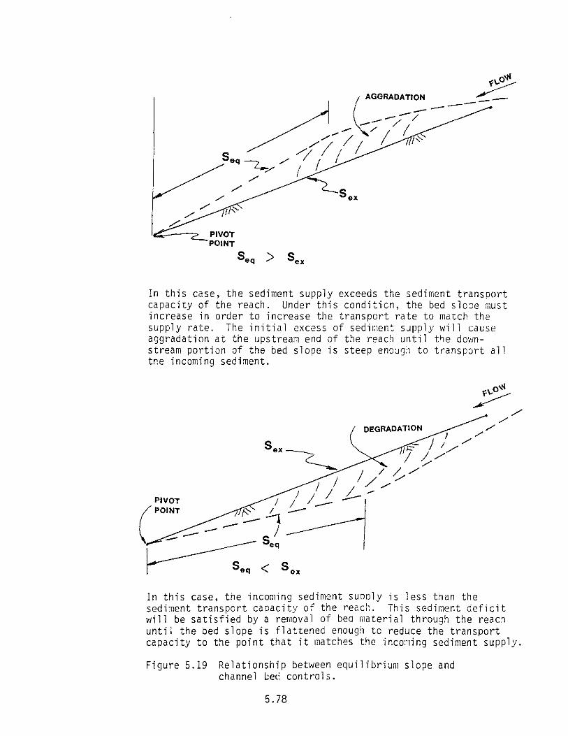
PIVOT'POINT
'eq > ex
In this case, the sediment supply exceeds the sediment transportcapacity of the reach. Under this condition, the bed slope mustincrease in order to increase the transport rate to match thesupply rate. The initial excess of sediment supply will causeaggradation at the upstream end of the reach until the down-stream portion of the bed slope is steep enough to transport allthe incoming sediment.
'ex
ox
In this case, the incoming sediment sunoly is less than thesediment transport capacity of the reach. This sediment deficitwill be satisfied by a removal of bed material through the reachuntil the bed slope is flattened enough to reduce the transportcapacity to the point that it matches the incoming sediment supply.
Figure 5.19 Relationship between equilibrium slope andchannel beci controls.
5.78

A summary of the equilibrium slope procedure is presented as follows:
1. Select upstream equilibrium supply reach and obtain the following data:
a. channel geometryb. channel slopec. sediment size distributiond. channel resistance (Manning's n)
2. Determine dominant discharge.
3. Divide the segment of the river system under analysis into separatereaches of similar hydraulic characteristics and identify control points.
4. Obtain the same information as in Step 1 for each downstream reach thatis to be analyzed.
5. Select an appropriate sediment transport equation (i.e., from Table 5.5if appl icable).
6. Establish the sediment supply provided by the upstream supply reach.This rate will be the sediment supply for all downstream reaches unlesssignificant tributary flow is encountered downstream of the supply reach.If equilibrium conditions can be assumed in the supply reach, the sedi-ment supply will equal the transport capacity of the supply reach.
7. Compute the sediment transport rate for each of the downstream reaches byvarying the slope through each reach until a transport rate is foundwhich matches the sediment supply. This establishes an equilibrium slopefor each reach.
8. Pivot equilibrium slopes about control points (if any were identified) todetermine long-term bed adjustment.
9. Check any degradation dimensions determined from Step 8 to see if themaximum stable bank height or armoring will control the amount of bedadjustment possible.
Example: Prior to the establishment of a strict flood plain management
program, residential development was allowed to encroach into the flood plainof a desert wash located in a rural area of Arizona.
In order to resolve the flooding problem for this community, a levee/channelization project has been proposed. The channel improvements will con-
sist of clearing vegetation from the exiting channel in order to lower the n
value to 0.025 as well as widening the channel to 200 ft.An equilibrium slope analysis is to be performed to determine the long-
term aggradation/degradation that may be induced by these channel improve-
ments. The results of this analysis will be incorporated into the design of
the bank stabilization system for the proposed levee.
5.79

1. A field inspection of the site indicated the wash had very uniform char-acteristics both up and downstream of the reach for proposed channelimprovements. Accordingly, the following channel parameters were con-sidered representative of both the upstream sediment supply reach and theexisting downstream reach which is to undergo channelization.
a. Existing channel bottom width is approximately 150 ft.b. Exist ing bed slope = 0.007 ft/ft.c. DSQ (bed material) = 0.5 mm.c. G (gradation coefficient) = 2.0.e. Average channel depth is about 4 ft.f. Existing channel n value was estimated at 0.04.
2. A hydrologic analysis of the upstream drainage area indicated the 10-yearevent has a peak discharge of 3,000 cfs. When Manning's Equation wasapplied to the supply section channel geometry with a discharge of 3,000c fs , the depth of f low was found to be about 3 ft. Since this is withina foot of being bankful l , 3,000 cfs was chosen as the dominant discharge.
3. The proposed channelization only extends along a 1,500-foot reach of thewash so the equilibrium slope analysis will be confined to this length.Since the existing channel conditions and proposed channel improvementsare uniform throughout this length, only one downstream reach will beused for the analysis.
An "at-grade" soil cement road crossing was discovered near the down-stream end of the study reach. It was assumed this crossing would with-stand the 100-year design flood, therefore it was to be a stable controlpoint for the equilibrium slope analysis.
4. The existing channel conditions through the study reach are listed inStep 1.
5. Referring to Tables 5.5 and 5.6a, it was determined that a power rela-tionship of the form qs = a Y^ Vc would be the most efficient way toanalyze the sediment supply and transport capacit ies through the reach.
From Table 5.6a, the fol lowing coeff icients and exponents were obtainedusing the data from Step 1:
a = 1.48 x 10"5
b = 0.0501
c = 4.31
Accordingly, the sediment transport equation is:
qs = 1.48 x ID'5 Y°'0501 V4 '3 1
5.80

Manning's Equation was used to compute the velocity and hydraulic depthfor the upstream sediment supply section. The following parameters fromStep 1 were used:
n = 0.04
b = 150 ft
side slopes = 1:1
bed slope = 0.007
Q = 3,000 cfs
The calculation yields V = 6.40 fpsyh = 3.00 ft
The sediment supply is now calculated as the transport capacity of theupstream supply section:
qs = 1.48 x 10"5 (3.00)0-0501 (6.40)4 '31
qs = 0.047 cfs/f t
Total sediment supply = q x average f low width
Q = (0.047H153)in
Q = 7.19 cfsi n
The transport capacity of the improved channel reach will now be computedwith different bed slopes until one is found which will yield a transportcapacity equal to the incoming supply rate. The proposed channel param-eters are as fol lows:
n = 0.025
b = 200 ft
side slopes = 1:1
Using the dominant discharge of 3,000 c fs, Manning's Equation is firstused to calculate the velocity and hydraulic depth for substitution intothe sediment transport equation. The calculat ions, which employ atrial-and-error sequence, are summarized in the fol lowing table:
5.81

Slope( f t / f t )
0.007
0.0025
0.003
0.00315
Yh
( f t )
1.92
2.61
2.47
2.44
V( f p s )
7.65
5.60
5.91
6.00
^S
( c f s / f t )
0.098
0.026
0.033
0.035
FlowW i d t h( f t )
204
205
205
205
QS( c f s )
19.99
5.33
6.77
7.18
A slope of 0.00315 yields a transport rate of 7.18 cfs which is approxi-mately equal to the incoming supply rate of 7.19 cfs. Accordingly, thiscan be taken as the equilibrium slope.
8. By pivoting the equilibrium slope around the downstream control point(soil cement road crossing), it is determined that up to 5.8 feet ofdegradation is possible at the upstream end of the channelized reach (seeFigure 5.20).
This long-term degradation should be added to any other anticipated ero-sion or scour to get a total toedown depth necessary to protect the leveefrom undermining. Additionally, this long-term degradation may initiatea headcut upstream of the channelized reach. For this reason, con-sideration should be given to placing a grade-control/drop structure atthe upstream end of the channel.
9. Backhoe pits were excavated to a depth of 8 feet at two locations in theexisting channel. No bed material was encountered of a size large enoughto form an armor layer. Accordingly, armoring will not limit the pre-dicted amount of long-term degradation.
5.3.8 Sediment Continuity Analysis
Discussion - The sediment continuity principle applied to a given channel
reach states that the sediment inflow minus the sediment outflow equals the
time rate of change in sediment storage. Mathematically, this can be pre-
sented as
n nQs. " qs .in out
5.82

1500'
0.007EXISTING SLOPE
-0.00315EQUILIBRIUM SLOPE
PIVOT POINT
NOT TO SCALE
Figure 5 .20 . Exist ing and Equil ibrium Slope Prof i lesfor Example Problem.
5.83

For a given discharge acting for a given time, the volume of sediment depos-
ited or eroded in a channel reach is simply the difference between the
upstream sediment supply rate (Qsjn) and the channel sediment transport rate(Qs ,). If the supply rate is greater than the transport rate, the reach isdepositional, while if transport is greater than supply, general scour will
occur. (The basic principle of the equilibrium slope analysis is no change in
volume, i.e., dVol/dt = 0 in Equation 5.10.)
The sediment continuity principle can be applied to analyze conditionsduring a single discharge (e.g. peak discharge of a 100-year flood) or during
the hydrograph of a single flood. Either of these applications provides
information on the short-term erosion/sedimentation occurring on a reach-by-
reach basis.
Appl ication - The first step in sediment continuity analysis is deline-
ation of the study reach into a number of subreaches. Delineation of sub-
reaches is based on (1) physical characteristics of the channel, such as top
width and slope, (2) hydraulic parameters, such as depth and, particularly,
velocity, (3) bed-material sediment characteristics, (4) areas of particular
interest to study objectives, such as bridges or locations of proposed channelimprovements, and (5) the desire to maintain reach lengths as uniform aspossible throughout the system. Items 1, 2 and 3 are generally selected to
provide consistency within the subreach, so that representative average con-
ditions may be determined. For example, consistency in top width and channel
length influence the utilization of sediment continuity results in evaluationof vertical channel response. As discussed in Section 5.3.9, erosion/sedi-
mentation volumes from sediment continuity are often linearly distributed
through the reach to determine vertical channel adjustments. Therefore, if an
upstream reach length is 2,500 feet and the downstream reach is only 1,500
feet, the vertical adjustment of the channel bed responding to the imbalance
in sediment supply and transport capacity between reaches will be much dif-
ferent from that had the downstream reach been dimensioned as 2,500 feet.
Furthermore, uniform channel lengths are important in maintaining the
integrity of sediment continuity analysis. Sediment continuity analysis does
not address the time or channel length that it takes for the difference be-
tween sediment supply and transport rate to achieve a balance. It is assumed
that a balance will be achieved within the reach regardless of its length.
5.84

This is not necessarily correct. For example, in a very short depositionalreach, particle settling times may not permit the calculated sedimentation to
occur. For this reason it is recommended that reach lengths be kept as uni-
form as possible to avoid the introduction of an additional variable to theanalysis that could bias or otherwise create unrealistic results.
After subreach delineation, characteristic geometric and hydraulicinformation must be developed for each subreach for the discharge(s) under
consideration. This information may be computed manually through uniform flow
or gradually varied flow calculations, or through computer programs such as
HEC-2. For example, if HEC-2 output data are available, the required velo-
city, depth and top width data at various cross sections within the study
reach will be provided. Within a given subreach these data can be averaged to
define values representative of conditions in that reach for the given
discharge.After establishing representative hydraulic characteristics in each
subreach for the given discharge(s), the sediment transport capacity of each
subreach is calculated using an appropriate method (see Section 5.3.6). The
sediment continuity principle is then applied by comparing transport capacity
on a reach-by-reach basis, under the assumption that the sediment supply to
any given subreach is equal to the transport capacity of the adjacent upstreamreach. The comparison begins at the upstream end of the study reach by
designating the first subreach as a supply reach, which initiates the calcula-
tion in Subreach 2.
Application of sediment continuity analysis to a flood hydrographrequires discretizing the hydrograph into a series of discrete discharges, as
described in Section 3.5. The reach-by-reach comparison is then completed for
each discharge and the total volume of erosion or deposition occurring in any
given reach during the flood is computed as VOL. = z (Q AT) where VOL. is
the net volume change during the flood for subreach i, Q is the excess
transport capacity or supply in subreach i for the given discharge (i.e.
supply minus transport capacity), and AT is the time interval corresponding
to that discharge from the discretized hydrograph. It is important to note
that this procedure yields a net volume of erosion or deposition that occurs
in response to passage of the complete flood hydrograph, i.e., we are looking
at the net change in volume at the end of the hydrograph. There may be time
intervals within the hydrograph where the volume change for that specific
5.85

interval would exceed the net volume change for the entire hydrograph. Thisis important to remember when using the sediment continuity procedure to com-
pute general scour, since an analysis of net changes at the end of a
hydrograph may under-estimate a transitory scour condition that might occur
during a critical time interval within the hydrograph.To expedite the calculation procedure when evaluating several hydro-
graphs, the following analysis procedure is suggested. First, identify fiveto ten discharges adequate to span the discharge range of all hydrographs.
After computing the average hydraulic characteristics in each subreach for
each discharge, compute the corresponding sediment transport capacities.
Then, for each subreach, develop a relationship of the form Q = a Q where
Q is the sediment transport capacity in cfs, Q is the water discharge in
cfs, and a and b are regression coefficients. The analysis of the discre-
tized hydrographs then proceeds as outlined aoove, with the sediment transport
capacity for any given discharge in any given reach obtained by using theappropriate regression relationship.
It is important to note that the sediment continuity analysis described
herein is based on the assumption of rigid-boundary conditions. For example,
during evaluation of a flood hydrograph, the channel geometry is assumed toremain unchanged throughout the flood. A more accurate analysis technique is
to update the channel cross sections for each discharge level of the flood to
account for the computed erosion/sedimentation changes. This concept is
referred to as quasi-dynamic routing, and is the basis of Level III analysiswhere computer models such as HEC-2SR are applied. However, for many prac-
tical engineering analysis and design problems the application of the sedimentcontinuity procedure is adequate and more cost efficient.
Example - As part of a channel stability study of tne Agua Fria River
near Phoenix, Arizona, a sediment continuity analysis was conducted for the
peak discharge of the 10- and lUO-year floods. This application of the sedi-
ment continuity procedure provided insight to the short-term response of the
channel. The approximate 30-mile study reach was divided into 10 reaches.
Average hydraulic and geometric characteristics for the 10 reaches were estab-
lished from i-IEC-2 analysis. For the 10-year flood peak the main channel velo-
cities ranged from 5 to 7 feet per second (fps) and for the 100-year, 7 to 10
fps. Sediment transport capacity was estimated by the Meyer-Peter, Muller
5.86

bed-load equation in combination with the Einstein suspended load procedure.
Reach 1 was utilized as the supply reach from which the sediment continuity
calculation began. Table 5.12 gives the results from the analysis and
indicates the general scour/deposition condition of each reach.
5.3.9 Quantification of Vertical and Horizontal Channel ResponsePi scus si on - Sediment continuity results provide the rate and/or volume
of erosion/sedimentation expected in each subreach. More meaningful results
are obtained when these values are converted to represent vertical and/orhorizontal changes in each subreach. Using the definitions established in
Section 5.1.2, sediment continuity results from a single flood would be usefulin quantifying general scour/deposition or short-term lateral migration.
Application - In the absence of significant controls the erosion/sedi-
mentation amounts can be assumed uniformly distributed in the streamwise
direction for any given subreach. If the cross-streamwise distribution is
also assumed uniform, then with knowledge of the reach length and by assuming
a representative channel width, typically top width, the uniform depth of ver-
tical adjustment can be evaluated. As an alternative, the cross-streamwise
distribution can be done according to flow conveyance; however, this can
become a tedious calculation by hand calculator.
In making the distribution, the computed sediment volumes must be
corrected for porosity. The sediment transport equations used in the sedimentcontinuity analysis give answers in unbulked volumes per unit time. A poro-
sity factor must be applied to these values to accurately represent the volume
changes that will occur in the channel bed. For sand-bed channels, a typicalporosity of n = 0.4 can be assumed. The unbulked sediment volumes computedby the transport equations are then corrected as follows:
Vt - Jlf (5.14)
where V is the bulked sediment volume, V is the sediment volume computedU ^
by transport equations, and n is the porosity.
Evaluation of lateral migration amounts is more difficult and not as sub-
jective to a rigorous analysis procedure as are vertical adjustments. The two
basic mechanisms of lateral migration can be related to erosion/sedimentation
5.87

Table 5.12. Short-Term General Scour/Deposition Response.
Reach
1
2
3
4
5
6
7
8
9
10
Qs (cfs)
105
112
187
122
158
131
168
81
80
106
10-Year&QS (cfs)
-7
-75
+65
-36
+27
-37
+87
+1
-26
Response
NearEquil ibrium
Scour
Deposition
Scour
Deposition
Scour
Deposition
Equil ibrium
Scour
100-YearQs (cfs) AQS (cfs)
379
254
446
541
581
538
676
465
446
492
+125
-192
-95
-40
+43
-138
+211
+19
-46
Response
Deposition
Scour
Scour
Scour
Deposition
Scour
Deposition
NearEquil ibrium
Scour
Qs is sediment transport rate, AQS is general scour ( - ) /deposi t ion (+)rates of the flood peak.
5.88

trends in the channel. The first mechanism, associated with channel reachesof large w/d (width/depth) ratio where significant sedimentation is
occurring, is that which promotes bank instability and lateral migration as a
result of increased velocities and shear stresses along the banks as the local
energy gradient increases. The second mechanism, associated with channel
reaches of small w/d ratio, typically in an erosional mode, is that which
causes increased bank instability from bank failures as a result of develop-
ment of a narrow, deep channel with steep banks.
There are several variations of the first mechanism involving channelswhere significant sedimentation is occurring. If sedimentation occurs as iso-
lated sand and gravel bars, the local energy gradient increases due to higher
flow velocities that result from a reduction in effective channel area.
Additionally, relatively stable sand and gravel bar deposits deflect the flowtowards the more erodible banklines. Consequently, severe localized bank
failures may occur. However, if deposition occurs more uniformly across the
channel, the local energy gradient downstream of the deposition increases due
to higher velocities resulting from an increase in channel slope. The absenceof current deflection and the more gradual increase in velocities results in
less severe bank erosion, but erosion takes place over longer distances.
Under either situation, quantifying lateral migration amounts from sediment
continuity calculations is difficult. Generally, in these types of reaches
the assessment of lateral migration potential must be made from qualitative
analysis such as historical evidence, meander scars, meander width, geomorphic
relationships, etc.There are also variations of the second mechanism involving a typically
erosional reach of the channel. The mode of bank failure as the channel deep-
ens depends on bank material composition. In a channel with predominately
clay banks, failure may be by sloughing due to undercutting by low-flow dis-
charges. In a stratified bank with lenses of erodible material, enough ofthis material may be removed that the block of bank material above tilts down-
ward, opening a vertical tension crack. Ultimately the bank fails in largeblocks. Piping can also promote bank failure in a stratified bank. Quantify-
ing lateral migration amounts for erosional reaches is easier than for reaches
where sedimentation is occurring. The volume of erosion computed from sedi-
ment continuity analysis can be assumed to come entirely from the channel
banks or can be distributed between bed and banks. However, since it is dif-
5.89

ficult to establish the distribution, and since the direction of lateral
migration is not known with certainty, it is sometimes appropriate to assume
the required volume first comes entirely from one bank and then the other.
The exception to this procedure is when controls inhibit movement in a given
direction. Additionally, it may be possible that the entire volume could come
from a single location on one bank, for example, a short-radius bend in rela-
tively erodible material.
In both mechanisms of lateral migration, development of saturated banks
above the water line can increase bank erosion through local mass wasting.
Saturated banks may develop during the rising stage of a flood, during which
flow moves into the bank from the river, promoting increased bank stability,
particularly in the saturated condition. Flow may also occur from the bank to
the river due to a groundwater table that is higher than the river stage.
This condition could develop during a wet period as water draining from the
watershed saturates the flood plain to a level higher than normal.
Example - A preliminary design for a sewer line in the City of Globe,
Arizona, proposed an alignment that followed the Final Creek channel for
approximately 3 miles. To evaluate the adequacy of the proposed 6-foot
burial, an erosion/sedimentation study was conducted. The study included
application of the sediment continuity concept to estimate erosion/sedimenta-
tion volumes, and then the conversion of these volumes to general scour/depo-
sition estimates.
The analysis was conducted for the 100-year flood (peak discharge 19,500
cfs). For simplicity, the hydrograph was discretized into three discharge
levels: one peak and two medium flows. The study reach was divided into
eight subreaches and, from a HEC-2 analysis, the average hydraulic conditionsfor each reach were determined. Sediment transport rates for each of the
reaches for all three discharges were then calculated, and the sediment con-
tinuity equation (Equation 5.13) applied between reaches to estimate the
erosion/sedimentation for each reach. The depth of general scour/depositionwas then determined by uniformly distributing the calculated volumes in each
reach. Table 5.13 presents the results and indicates as much as 9 feet of
general scour is possible; therefore, the 6-foot burial depth was not con-
5.90

Table 5.13. Sediment Continuity Results.(100-Year Flood)
AveragePotential
Bed Level ChangeReach (feet)
1
2
3
4
5
6
7
8
+ 4.8
+ 8.3
- 9.4
+ 1.2
- 5.9
- 0.5
- 4.3
Supply Reach
5.91

sidered adequate unless some type of channelization or grade control was to beimplemented in Reach 3.
5.3.10 Lo_cal Scour Concepts
2i_sc_us_s_i_0]i - Local scour is observed whenever an abrupt change in the
direction of flow occurs, such as at bridge piers or embankments. For
example, local scour at bridge piers is a result of vortex systems developed
at the pier. Local scour occurs when the capacity of the flow to remove or
transport the bed materials is greater than the rate at which replacement
material is supplied.
During a flood, an equilibrium condition between sediment supply and
transport capacity at a scour hole may never become established. During the
rising limb of the hydrograph scour occurs and endangers the hydraulic struc-ture. After the peak has passed (during the falling limb), the scour hole
refills as sediments drop out with the lower flows. Therefore, the critical
time for structural stability during the storm is near the peak flow (see
Figure 5.21). Soundings made of scour holes after the storm do not indicatethe potentially dangerous situation that might have existed during the storm.
The depth of scour also varies with time depending upon the presence or
absence of bed forms. The time required for dune or antidune motion is much
larger than the time required for local scour. Thus, even with steady-state
conditions, the depth of scour is likely to fluctuate with time when there are
dunes or antidunes traveling on the channel bed. The depth of the scour hole
is more variable with larger bed forms. When the crest of the dune or anti-
dune reaches the local scour area, the transport rate into the hole increases,
the scour hole fills and the scour depth temporarily decreases. When a trough
approaches, there is a smaller sediment supply and the scour depth increases
to try to re-establish equilibrium in sediment transport rates. A mean scourdepth between these oscillations is referred to as equilibrium scour depth.
Application - A number of formulas are available for predicting local
scour around bridge piers. Review of these formulas indicates that each is
based on those factors that seem most important in evaluating local scour at
bridge piers; however, most of these formulas are based primarily on model
study data in sand-bed laboratory flumes with little or no field verification.
Therefore, it is generally advisable to utilize several formulas to insure a
5.92

Q.O>Q
StormHydrograph
Time
Scour depthat bridge
Time
critical time
Figure 5.21. Temporal change of scour holedepth during a storm (typicaV
5.93

reasonably accurate estimate. Several of these formulas have been found to be
particularly successful based on previous experience. A relationship for
square-nosed piers presented by Richardson, et al . (1975) is
A7 h °'65
9 o I ^ c ' ,c ic ^-y — = 2.2 (— ) Fr (5.15a)
and for a group of circular cylinders
AZ b °'65
<?s p n 4^-y^ = 2.0 (--} Fr 4J (5.155)
where AZ is the e q u i l i b r i u m depth of the scour ho le , bp is the pierX» *3 r
width (normal to the flow direction), Y is the upstream depth of flow, and
Fr is the upstream Froude number (Fr = V//gY~ with V the upstream velocity
and g the acceleration of gravity).
The equations by Shen et al . (1966, 1969) for circular piers are
AZ£S = 0.00073 Rp' (5.16a)
and
AZ£S 2-^=11.0 Fr£ for Frp < 0.2 (5.16b)Dp
-£$. = 3.4 Frp°<67 for F^ 0.2 (5.16c)
respectively, where Rp is the pier Reynolds number (V bp/v), V is the
mean velocity of the undisturbed flow, bp is the width of pier projected on
a plane normal to the undisturbed flow, v is the kinematic viscosity, and
Frp (pier Froude number) is V//gbp .
The shape of the pier is a very significant parameter with respect to
scour depth because it reflects the strength of the horseshoe vortex at the
base of the pier. A blunt-nose pier causes the deepest scour. Streamlining
the front end of the pier reduces the strength of the horseshoe vortex, thus
reducing the scour. Streamlining the downstream end of piers reduces the
strength of wake vortices. Common shapes of piers are shown in Figure 5.22.
The scour depth generally decreases as a consequence of streamlining, while
5.94

Vbp c % (•>»— *
(a ) Squore- nose (b ) Round-nose ( c ) C y l i n d e r
• < > bp o a(d ) Shorp - nose (e) Group of Cyl inders
Figure 5.22. Common pier shapes.
5.95

skewed pier alignment (pier not parallel with flow direction) will create
deeper scour holes. The reduction due to streamlining can be estimated fromTable 5.14, while the increase due to skew can be determined from Figure 5.23
(Factor K . ). As previously indicated, the maximum scour depth can be con-3L
siderably greater than the equilibrium scour depth due to dune bed forms.
Richardson, et al . (1975) suggest that scour depths can be up to 30 percentgreater as a consequence of bed forms. Therefore, when dune or antidune bed
forms are possible, a safety factor of 1.3 is recommended, unless the magni-
tude of the dune or antidune bed forms is calculated as a separate component.
Another important local scour zone at a bridge crossing occurs at the
abutments. Detailed studies of scour around embankments have been made only
in laboratories. For example, Liu, et al . (1961) investigated scour around
vertical wall embankments for subcritical flow in a rectangular laboratory
flume with sand-bed conditions and found
AZ£s . 1C /a,0'4 r 0.33 lc ... .~Y — = 2.15 (y) Fr (5.17a)
where Y is the upstream normal flow depth, a is the embankment length(measured normal to the wall of the flume in the model studies), and Fr isthe upstream Froude number (using the upstream normal flow depth as length
dimension). Liu, et al . also presented limited data for spill-through embank-ments, where a spill-through embankment has sloping sides (i.e. the more com-
monly constructed earthen embankment). Analysis of the data presentedsuggests the equation
AZ£S 1 1 ,a>°'4 _ 0.33 ,_ ,_..~Y — = 1.1 (y) Fr (5.17b)
Richardson et al . (1975) suggest that Equation 5.17b be applied only for
embankments where a/y is less than 25. For embankments where a/y is
greater than 25, the equation
> = 4Fr°'33 (5.18)
is recommended. This equation was developed from field measurement of embank-
ment scour at rock dikes on the Mississippi River. It is worthwhile to note
that embankment scour equations are also useful for estimating local scour at
bank protection, spur dikes and jetties.
5.96

Table 5.14. Reduction Factors When Applying Formulasfor Square Nose Piers to Other Shapes(assuming equal projected widths of piers)
Type of Pier Reduction Factor
Square nose 1.0
Cylinder 0.9
Round nose 0.9
Sharp nose 0.8
Group of cylinders 0.9
5.97

' 7
Multiplying Factorsfor
30 45 60Angle of Attack in Degrees
Figure 5.23. Scour increase factor, KaL, with flow
(from Lauren and Toch, 1956).
5.98

Une of the difficulties in applying Equations 5.17b and 5.18 is defini-
tion of "embankment length." Model study investigations considered only short
embankment lengths in smooth, rectangular flumes. In prototype situations,
the embankments may span large distances across the overbank of a wide flood
plain while stopping short of, or just slightly protruding into, the main
channel. Due to the normally large difference in hydraulic characteristicsbetween main channel and overbank flow, caution must be exercised in defining
the embankment length for such cases. Figure 5.24 illustrates a recommended
embankment length definition for different cases that may be encountered out-
side the realm of a rectangular laboratory flume. For Case 2 of Figure 5.24,
the engineer should compute embankment scour using main channel hydraulics
with the value of a. , and compare this result to that obtained using over-
bank hydraulics with the value for a,, . The larger of these two scour depths
would be the recommended design value. Due to the sensitivity of Equations
5.17a, 5.17b, and 5.18 to embankment length, engineering judgment should
always be applied.
Another difficulty common to any scour calculation is the definition of
the base level, and its relation to both flow depths and scour depths. In a
nonprismatic natural channel, the upstream normal depth (Y) is generally
defined by the hydraulic depth (Y. ) for purposes of scour calculations, while
the computed scour amounts are referenced to the thalweg elevation. If dunesexist, the upstream normal depth would generally be referenced near the top of
the dunes (in consideration of effective flow area), while the scour amounts
should oe referenced to the bottom of the dunes. In the presence of degrada-
tion and/or general scour, the ultimate bed invert elevation should first be
established for these scour components, from which local scour depths are then
referenced.Once the scour depth is accurately established, the lateral extent of the
scour hole is nearly always determinate from the depth of scour and the
natural angle of repose of the bed material. A safety factor of 2 should beapplied to the lateral scour hole dimension to account for nonuniform flow
conditions. This can be accomplished by dividing the angle of repose by 2 and
using the resulting angle to define the sides of tiie scour hole.
Example - The design of two bridge crossings on the Canada del Oro Wash
near Tucson, Arizona, required the evaluation of local scour around the bridge
5.99

CASE 1Overbank Levee
Upstream depth of flow,Y, and Froude numbershould be based on hyd-raulic conditions for rightoverbank flow.
CASE 2Bridge Embankment
Upstream depth of flow,Y, and Froude numbershould be based on hyd-raulic conditions for mainchannel f low when usinga-j and overbank flowwhen using &2- Acomparison of scourcalculations using thesetwo definitions ofembankment length isrecommended.
Fiqure 5.24. Definition sketch of embankment length "a".
5.100

piers. Each bent consists of four piers , a l igned paral le l to the f l o w ( i . e . ,
no skew) , and each pier was a concrete cyl inder three feet in diameter. The
design condi t ions are stated as f o l l o w s :
Q10Q = 33,000 cfs
Y (average depth of f l o w ) = 6.0 feet
V (average veloci ty) = 18.2 fps
A review of h i s tor ica l photos taken d u r i n g f lood stage at other br idge
locat ions on the Canada del Oro indicates that two add i t iona l feet of debris
b u i l d u p beyond the normal pier width could be expected d u r i n g a 100-year
event. A c c o r d i n g l y , the e f fec t ive pier w id th was set as f o l l o w s :
b = pier diameter + 2 = 3 + 2 = 5
Local scour was computed wi th Equa t ions 5.15b, 5.16a and 5.16b. The com-
pu ta t ions are shown as f o l l o w s :
b 0.65 n ...E u a t i o n 5.15b: AZ. = 2 . 0 Y ( ) Fru '^ J
Y and b are given above.
Fr = _±_ = __ L8_i2_ = 1 31> * J» * +J X
/gT /3T.2 x 6.0"
Subs t i t u t i ng in Equa t ion 5.15b:
AZ^ s = 2.0 ( 6 . 0 ) (g\)°'65 (1.31)0 '43 = 12.0 feet
Equa t ion 5.16a: AZ£$ = 0.00073 R°'619
Vbwhere R = — —
P v
-5 2with an assumed water temperature of 70"F, v = 1.059 x 10 ft /sec,
therefore, R = -(l8-2-l(AL = 8.5 x 10⁶
p 1.059 x 10"D
Subs t i tu t ing in Equa t ion 5.16a,
5.101

AZn = 0.00073 (8.5 x io6)0'619 = 14.2 feet
Equation 5.16b: The pier Froude number, Fr , must first be calculated_ pto determine which form of Equation 5.16b should be used:
Fr =p /gb~~ /32.2 x 5
Since Fr > 0.2, the fol lowing equation is used:
= (3 .4H5H1.43) 0 - 6 7 = 21.6 feet
summary of the ca l cu l a t i on is presented as fo l lows :
Eq. 5.15b Eq. 5.16a Eq. 5.16b
Local equilibrium 12.0 ft 14.2 ft 21.6 ftscour depth
Average = 15.9 ft
Considering the average of the three calculations, 16 feet of local scourcould be expected during the design flow. However, because of the similarity
of two of the three estimates, it is reasonable to assume that the equilibriumscour depth will probably be less than 16 feet.
5.3.11 Contraction ScourPi cussion - Contraction scour was defined in Section 5.1.2 as a special
case of general scour. Scour at a contraction occurs because the flow areabecomes smaller than the normal channel and the average velocity and bed shearstress increase, hence there is an increase in stream power (iV) at the con-
traction and more bed material is transported through the contracted sectionthan is transported into the section. As the bed level is lowered, velocity
decreases, shear stress decreases and equilibrium is restored when the trans-
port rate of sediment through the contracted section is equal to the incoming
rate.
5.102

Application - Evaluation of contraction scour is by application of the
sediment continuity principle for conditions after equilibrium has been
achieved. That is,
Q- = Q- (5.19)sl S2
where Qs, is the sediment transport capacity at the upstream section and
Qs2 is the value at the contraction. When the sediment transport capacity isexpressed in the form of power functions (e.g. as given in Tables 5.6a, 5.6b
and 5.7), the relationship is
a vj vj W1 = a Y2 V2 W2 (5.20)
Through manipulation and simplification of this equation, a relationship for
the flow depth Y2 (after equilibrium is established) can be derived as
q -L-- -b"C (5.21)
a q2
where
Wqc = rp qc (where q = a Y^ V^) (5.22)S2 W2 sl sl
and
W,q2 = yi qj_ (5.23)
The amount of general scour is then the difference between the pre-scour flowdepth and that value from Equation 5.21 after equilibrium had been achieved,
i .e.,
AZ = Y2 - Y2 (5.24)
where AZ is the general scour depth and Y'? is the original flow depth
at the contraction.If the site under investigation has hydraulic and sediment properties
that fall outside of the limits listed in Tables 5.6a, 5.6b and 5.7, a set of
regression coefficients (a, b and c) should be developed for the specific
5.103

condi t ions at that site. For example, this regression ana lys i s can be per-formed by u s i n g the Meyer-Peter, M u e l l e r bed-load equat ion in combina t ion wi th
the E i n s t e i n suspended-load methodology to compute the u n i t wid th bed-materialload transport rate for a range of discharges at the site under i n v e s t i g a t i o n .
Each u n i t t ransport rate is then regressed aga ins t the cor responding veloci tyand depth parameters for the g i v e n water d ischarges ( e . g . as e s t ab l i shed f rom
HEC-2 resul ts) . The results of this regression analysis yield values for a,b and c ( d e s c r i b i n g the equa t ion q = a Y, V ) w h i c h can then be used in
the above cont rac tua l scour a n a l y s i s . As a less time c o n s u m i n g and less site-spec i f i c a l t e rna t ive to the regression ana lys i s approach, the eng inee r may optto u t i l i z e the scour equat ions presented on pages 58 through 62 of Sedimenta-tion E n g i n e e r i n g , ASCE Hanua l s and Reports on E n g i n e e r i n g Practice Wo. 54
(1975) .
Examp1e - Construct ion of a bridge w i l l result in a reduction in channel
wid th from 320 to 240 feet. Water-surface p r o f i l e ana lys i s wi th the b r idge inp lace e s t a b l i s h e d veloci ty and depth in the reach upstream of the proposedb r i d g e as 8.6 fps and 10 feet, respect ive ly , for a peak d i s cha rge of 27,500
cfs . S i m i l a r i l y , at the br idge site the ve loc i ty and depth were computed as
10.2 fps and 11.2 feet , respect ively .C o n s i d e r i n g the bed-mater ia l charac te r i s t i c s , the a p p r o p r i a t e e m p i r i c a l
power r e l a t i o n s h i p for sed iment t ransport ( T a b l e 5 .6a ) i s
qs = 3.45 x ID'6 Y-°'693 V 4 ' 6 0
Therefore, the u n i t sediment discharge upstream of the br idge is
q = 3.45 x ID'6 dor0'693 (8.6)4 '6 0
Sl
= 0.014 c f s / f t
and at the br idge site
320 M m , cfs\ = 2WU ' 0 1 4 TT
= 0.019
5.104

The un i t water discharge at the bridge site is
Q = 320 (27 ,500 . =q2 240 ( 320 ' i iH '°
The f l ow depth at the br idge site after e q u i l i b r i u m is
1_ , 0.019 v -0.693-4. 60_ _
2 3 .45xlO~ 6 (114. 6) 4 ' 6 0
= 12.1 ft
The amount of scour is then
AZ = 12.1 - 11.2 = 0.9 ft
5.3.12 Bend ScourDiscussion
The bends associated with meandering channels will induce transverse or
"secondary" currents which will scour sediment from the ouside of a bend andcause it to be deposited along the inside of the bend. It is important tonote that this scouring mecnanisin is caused by the spiral pattern of secondary
flow, and is not due to a shift of the maximum longitudinal velocity filament
against the outer bank. Channel bends will cause a shift in this velocityfilament, but through the bend the maximum longitudinal velocity is normallymoved nearer to the inside bank, whereas the shift to the outer bank occursdownstream of the bend. It is at these downstream locations that the shift in
longitudinal velocity patterns will most likely cause lateral erosion of achannel bank.
The discussion presented in this manual will address the vertical scourpotential in a channel bend. A review of technical literature will reveal the
existance of several theoretical relationships that have been developed topredict the amount of scour through a river bend. To date, there is no knownprocedure which consistently yields an accurate prediction of bend scour
through a wide range of hydraulic and geometric conditions. Based on the
assumption of constant stream power through the channel bend, Zeller (1981)developed the following relationship for estimating the maximum scour com-
ponent resulting from channel curvature in sand-bed channels:
5.105

A7 0.0685 YV°'8AZbs= TTT--Yh ^e
where AZtjS = bend scour component of total scour depth (feet)
V = mean velocity of upstream flow (fps)Y = maximum depth of upstream flow (feet)
Yn = hydraulic depth of upstream flow (feet)
Se = upstream energy slope (bed slope for uniform flow conditions,
feet/feet)a = angle formed by the projection of the channel center!ine from
the point of curvature to a point which meets a line tangent to
the outer bank of the channel (degrees, see Figure 5.25)
Mathematically, it can be shown that, for a simple circular curve, the
following relationship exists between a and the ratio of radius of curvature
to channel topwidth.
_ - _U 9 n 'W 4 siV(f)
where rc = radius of curvature to centerline of channel (feet)
W = channel topwidth (feet)
If the bend under evaluation deviates significantly from a simple cir-
cular curve, the engineer should consider dividing the bend into a series of
circular curves and analyzing the bend as a compound curve. Under this proce-
dure, there would be a different value of a determined for each segmentof the compund curve. A scour depth would then be computed for each segment
of the curve using the a determined for that segment.
ApplicationEquation 5.25 can be applied to natural river bends to get an approxi-
mation of the scour depth that can be expected in the bend during a specific
water discharge. The impact that other simultaneously occurring phenomena
such as sand waves, local scour, long-term degradation, etc., might have on
bend scour is not known for certain. In order that the maximum scour in a
5.106

TANGENT TO CURVE
CHANNEL
CENTERLINE
CENTER OF CURVATURE
Figure 5.25 Illustration of terminology for bend scour calculat ions.
5.107

bend not be underestimated, it is recommended that bend scour be considered asan independent channel adjustment that should be added to those adjustments
computed for long-term degradation, general scour, and sand wave troughs.
Whether or not bend scour should be added on top of local scour would depend
on the type of obstruction creating the local scour. For isolated structures,such as transmission towers, that would not appreciably disrupt the secondary
flow pattern responsible for bend scour, it would be recommended that bend
scour and local scour be computed separately and added together. For the case
of a series of armored spur dikes placed along the outside bank of a bend, thespiral flow pattern may be disrupted to the point that significant bend scour
would not occur. Engineering judgement would have to be exercised in such
cases when computing the total vertical scour that might occur in the channel
bed.
The longitudinal extent of the bend scour component is as difficult to
quantify as the vertical extent. Rozovskii (1961) developed an expression for
predicting the distance from the end of a bend at which the secondary currents
will have decayed to a negligible magnitude. This relationship is:
X = 2.3 (-£— ) Y (5.27)
where X = distance from the end of channel curvature (point of tangency, P.T.)to the downstream point at which secondary currents have dissipated
(feet)
C = chezy coefficientg = gravitational acceleration (32.2 feet/second2)
Y = depth of flow (to be conservative, use maximum depth of flow, exclu-sive of scour, within the bend) (feet)
Equation 5.27 should only be used as a guide in determining the distance
downstream of a curve that secondary currents will continue to be effective in
producing bend scour. As a conservative estimate of the longitudinal extent
of bend scour, both through and downstream of the curve, the engineer would be
advised to consider bend scour commencing at the upstream point of curvature
(P.C.) and extending a distance X (computed with Equation 5.27) downstream of
the point of tangency (P.T.) Engineering judgement should be used in electing
to deviate from this generalized recommendation.
5.108

Example
Proposed channel improvements on a river system include the installation
of soil-cement on the channel banks to prevent bank erosion. The river reach
where these improvements are to be installed includes a channel bend which has
the following hydraulic data:
Y = 9.39' Se = 0.0013 ft/ft
V = 12.62 fps a = 24°
Yn = 9.18' n = 0.025
In order to prevent undermining of the soil cement bank protection, it is
desired to extend the soil -cement a certain distance below the natural channel
bed. This toe-down depth will include allowances for long-term degradation,
general scour, sand wave troughs and bend scour. The maximum bend scour com-
ponent of the toe-down depth is computed as follows:
0.2
A7 0.0685 YV°'8 ,, . ,sin2 7, .AZbs= 0 . 4 0 . 3 L2-1 ( ) - 1
A7 - 0.0635 (9 .39) (12.62)0 '8 r? . ^s in 2 ^ 0 ^ , ,
"fc-W ~* --------- . .. - _ - --------------- .-.. ,.:..... -,-, --------- - .- . , . ", — | £. • X \ ™™ -,,- .y- I — j_ j
DS (9.18)U-4(0.0013)U";i cos 24
AZbs= 2.09 feet (use 2.1 feet)
This dimension (2.1 ft) will be added to any other computed vertical bed
adjustments (general scour, sand wave troughs, etc.) for the curved portion of
the channel. The distance downstream of the curve to which the bend scour
component will be applied, is computed using Equation 5.27.
x = 2.3 (— ) Y
wnere
For the design flow, the hydraulic radius, R, was determined to be 9.03
feet. Accordingly, C is computed as follows:
5.109

C =iil8! (0.025
C = 85.77
Subs t i tu t ing into E q u a t i o n 5.27
X = 2.3 (-M
^X = 319 feet
Therefore, the bend scour component (2.1 feet) w i l l be app l i ed to thesoil-cement toe-down depth th rough the entire curve and for 319 feetdownstream of the point of tangency of the curve.
5.3.13 E v a l u a t i o n of Low-Flow C h a n n e l Inc i sements
Discuss ion - When large width-depth ratios exist , cons idera t ion shou ld be
given to the development of low-f low channe ls . For example, a channel formed
predominan t ly by a 5-year to 10-year f lood w i l l develop width and depthcharacterist ics to carry this re la t ive ly large discharge in a h y d r a u l i c a l l ye f f i c i e n t manner ; however , for sma l l e r f loods these channe l d i m e n s i o n s may
resul t in a f l o w pattern a p p r o a c h i n g sheet f l o w c o n d i t i o n s . Rather thancar ry ing the f l o w in th is m a n n e r , the channe l w i l l deve lop a l o w - f l o w channe lthat provides more e f f i c i en t conveyance of the low- f low discharges. The
development of a low-f low channel w i l l create entirely d i f f e r en t hydrau l iccondi t ions than those occurr ing in the o r i g i n a l channe l geometry, and maycreate bank i n s t ab i l i t y from inc i semen t . Therefore, i t is impor tant for theengineer /des igner to ant ic ipa te the potent ia l for l o w - f l o w c h a n n e l i nc i semen t .
A p p l i c a t i o n - There are no r igorous methodolog ies for the p r ed i c t i on oflow-f low channel inc isement . A f i e l d inspect ion of the study area is probably
the best method to determine the potential for low f low channe l inc isement .
If the existing channel has developed a low-f low channe l , then it is appropri-
ate to use the observed i n c i s e m e n t depth for des ign purposes . If the ex i s t i ng
channe l does not have l o w - f l o w i n c i s e m e n t , but proposed c h a n n e l i z a t i o n or
other changes resul t in cond i t i ons f a v o r a b l e for l o w - f l o w c h a n n e l deve lopmen t ,
then as a ru le of thumb a reasonable inc i semen t depth ( A Z . ) is one to two
feet. The incisement depth should be added to any other vertical channel
5.110

adjustment that is used to determine the burial depth of piers, pipelines,bank stabilization, etc.
5.3.14 Evaluation of Gravel Mining Impacts
Pi scussion - Common gravel mining practices in arid areas includeinstream mining, flood-plain mining and terrace mining. Instream and flood-
plain mining activities have potential impacts on the river response andrequire adequate hydraulic, erosion and sedimentation analyses to develop an
acceptable mining plan. For example, sand and gravel mining may affect the
sediment movement and supply in a channel system. Such operations can bebeneficial or detrimental, depending on watershed and river characteristicsand on the mining and management practices followed.
Excessive sand and gravel removal from a river channel (removal greater
than supply in any given reach) can endanger the stability of the river system
and bridges by inducing general scour and headcutting. For example, bridges
over the Salt, Gila and Agua Fria Rivers have been endangered during floods
due to significant bed erosion and/or lateral migration of channels. Sand and
gravel mining in the river channel has been identified as a contributor to
documented bridge instability and/or failure. Analysis of the effects of sand
and gravel mining on the stability of a river system and bridges is important,
and protection of the bridges may be required where the sand and gravel mining
is of significant magnitude.On the flood plain adjacent to the river channel many of the same pro-
cesses are at work; however, impacts are generally restricted to overbank
flooding conditions. Water and sediment transport rates over the flood plainare generally reduced by the influence on resistance to flow of such
flood plain features as vegetation and structures. Just as headcutting aboveinstream gravel pits can endanger upstream bridges, erosion of flood plain
gravel pits could encroach on adjacent properties or threaten nearby struc-
tures. Of equal concern when flood flows spill over into a gravel pit is thepotential erosion of a dike or buffer zone designed to separate the pit from
the active river channel. A headcut and erosion through such a buffer zone
could alter local river channel characteristics and transport rates, and
impact both upstream and downstream reaches. If the channel reach adjacent to
a flood plain gravel pit is geomorphically active, e.g., migrating laterally,
5.111

the same result might occur if protective measures or an adequate buffer zone
are not provided during site development.
Application - The extent of damage to the system that can result from a
headcut induced by sand and gravel mining is a function of volume and depth of
the gravel pit, location of the pit, bed-material size, flood discharge, and
sediment inflow rates and volume. The presence of an instream gravel pit can
add energy to the system by increasing the water-surface slope, or energy
slope, just upstream of the pit. The steeper slope has greater erosive powerand can initiate bank erosion and headcutting. These processes can tip thebalance of sediment transport and induce degradation just upstream of the pit
and aggradation in the pit. When storm runoff impinges on the gravel pit the
energy slope, flow velocity and sediment transport capacity increase at theupstream boundary of the gravel pit and then attenuate in the gravel pit. In
response to the changes of sediment transport capacities at the pit boundary,
the channel initiates bank sloughing and/or downcutting upstream of the pit.
Furthermore, since the velocity of flow through the pit is negligible compared
with both the flood-plain and main channel velocities, tne pit will act as a
sediment trap. Due to this lowered velocity, water leaving the pit does not
have the capacity to carry sand- and gravel-sized material. This relatively
sediment-free water will flow back into the main channel downstream, and thus
the possibility of general scour due to the introduction of clearer water into
the main channel must be considered.
The length of time during which conditions are favorable for bank erosion
and headcutting depends on the volume of the pit and on the inflow hydrograph.
For a low-flow event an instream pit will not fill or reach equilibrium as
soon as it will during a high-flow event. During a high-flow event the rising
limb of the hydrograph rapidly fills the pit with water and drowns out theeffect of a steeper energy slope. This concept is illustrated in Figure 5.26
for representative low- and high-flow hydrographs. The crosshatching indi-
cates the relative times required to fill a gravel pit to the level where
channel hydraulics control the flow conditions.
For a gravel pit in the overbank, low flows are generally not of concern.
Flood flows will not be of concern until overbank flows occur. While overbank
flows are filling a flood plain gravel pit, the same potential exists for
headcutting and erosion as with an instream pit; however, once the flood plain
pit is filled, it will constitute only a pool or slack-water area on the flood
5.112

Low Flow Event
In-stream Pit
Time
High Flow Event
In-stream Pit
Time
Figure 5.26. Relative time for filling a gravel pit and reachingequilibrium for a low and high flow event.
5.113

plain. The central segment of the hydrograph, then, is critical to the stabi-lity of a flood plain pit. This concept is illustrated in Figure 5.27, in
which the crosshatched area represents the time between overbank spill intothe pit and final filling of the pit.
The scour and deposition problems associated with sand and gravel mining
are very complicated. Simplifying assumptions are needed to obtain a prac-
tical and economical solution. The dominant physical processes include water
runoff, sediment transport, sediment routing by size fraction, degradation,
aggradation, and breaking and forming of the armor layer. These processes are
unsteady and complicated in nature. Furthermore, each situation is unique and
requires independent analysis. No standard procedure can be adopted which is
universally applicable to all gravel mining evaluations. However, some typi-
cal steps that might be required to analyze a headcut profile upstream of a
gravel pit would include:
1. Selection of a design hydrograph. Several hydrographs may be evaluatedto determine the sensitivity of the gravel pit to different size andshapes of hydrographs.
2. Determine gradation of bed material.
3. Compute hydraulic parameters (velocity and depth) for a range of slopevalues and the anticipated headcut geometry.
4. Determine unit discharge sediment transport relationship representativeof the conditions identified in Steps 2 and 3.
5. Dimension pit geometry for beginning of flood conditions.
6. Select upstream sediment supply cross section and develop transportequation.
7. Route discretized hydrograph through sediment supply section and gravelpit. Adjust bed profile upstream and downstream of the pit entrance atthe end of each time step to balance the volume of material eroded fromthe upstream edge of the pit with the volume of material deposited withinthe pit.
Example - An instream sand and gravel mining operation just downstream of
the Oracle Highway Bridge over Rillito Creek in Tucson, Arizona, was analyzed.
The reach length studied was approximately two miles (river rnile 4.00 to 6.1),
with the bridge located at river mile 5.05. The gravel pit extended from mile
4.65 to 5.03. Assumed dimensions of the pit for analysis purposes were
10 feet deep by 400 feet wide by approximately 2,000 feet long. Upstream of
5.114

High Flow EventFloodplajn Pit
CT
O
Time
Figure 5.27. Critical time for erosion of a floodplain gravel pit.
5.115

the bridge the channel is 350 feet wide. Five cross sections were used within
the pit to define the geometric conditions.The hydrograph used for testing was the two-year flood event with a peak
discharge of 7,000 cfs. The 18-hour duration was divided into six time steps
of three hours each. The changes occurring in the geometry of the upstream
edge of the pit were defined at each of these time increments.
The inital condition was a dry river bed and an empty gravel pit (i.e.,
no water). Prior to filling the pit with water and sediment, a normal depth
approximation was used, rather than the HEC-2 analysis, to determine the
hydraulic conditions and sediment transport rate needed for the headcut pro-file calculations. After the pit filled with water, HEC-2 analysis was used
to define the hydraulic conditions. The inflow occurring during the first
time step (three hours) initiates the headcut by eroding the corner off the
upstream edge of the pit and depositing sediment in the bottom of the pit at
the upstream end (Figure 5.28). The slope of the headcut and deposited
material is 0.050; however, a discontinuity of 2.40 feet exists. At time 5.20
hours the discontinuity between the headcut and deposition slope disappears
and a continuous slope of 0.050 exists. The changes occurring throughout thehydrograph are illustrated in Figure 5.28. The pivot point actually shifted
upstream 18 feet, although the resolution on the figure does not illustrate
this. The calculated scour occurring at the bridge as a result of the headcut
was 4.7 feet at the end of the storm, which is consistent with actual soun-
dings that indicated approximately five feet of general scour for this event.
5.3.15 Cumulative Channel AdjustmentDj_scussion - The potential vertical adjustment of the channel bed in any
given reach is determined from consideration of all the possible incremental
adjustments. For example, it is possible that a given reach will be simulta-
neously degradational while local scour and contractual scour are occurring at
the bridge crossings. In this situation the three erosion components would
have to be accounted for to establish the ultimate bed elevation.
Application - The cumulative channel adjustment at any given location is
the summation of six possible components:
5.116

Eiapseo Time (hours)
5 6 9 2
Note' Not 10 scale
Figure 5.28. Definition sketch of the temporal changesat the upstream edge of a gravel pit.
5.117

AZtot = AZdeg + AZls + AZgs + AZbs + AZi + 7 ha (5'28)
where AZ, " . is the total vertical adjustment in bed elevation, AZ, is
the change from long-term degradation (Section 5.3.9), AZ, is the local
scour depth (Section 5.3.10), AZ is any relevant general scour depth
(e.g. Section 5.3.11 or 5.3.14), AZ, is the bend scour depth (Section
5.3.12), AZ. is the low-flow incisement depth (Section 5.3.13), and h isi athe antidune wave height (Section 4.6.2). As a conservative practice, any
long-tern aggradation amount that might mitigate some elevation decrease isnormally not considered.
Due to the complex interaction that will occur among these six phenomena,it is perhaps impossible to accurately predict the total cumulative bed
adjustment that might occur at a given location. The hydraulic parameters(velocity, depth, top width, etc.) that are used to compute the dimension of
each phenomenon will constantly change as this interaction proceeds; however,
the parameters that are used in the calculations are normally based on rigid-
bed conditions which give no consideration to channel geometry changes thatmay be initiated as a result of the simultaneous occurrence of all or part of
the six phenomena. Accordingly, the application of a factor of safety to the
total computed vertical adjustment (AZ .) is very judgmental, i.e., no firm
value can be recommended. In deciding to apply a factor of safety to the com-puted result, the engineer should consider the magnitude of damage that might
accompany a design failure, the probability or risk that such an event might
occur, the construction cost associated with applying a safety factor, and the
reliability of the data that were used in the channel adjustment calculations.Depending upon the answer to such questions, typical safety factors will pro-
bably range from 1.0 to 1.5.
Example - In the example of Section 5.3.9, a potential degradation of 9
feet was calculated for Reach 3 of the Final Creek channel. For purposes of
illustration, assume a bridge crossing in this reach produces local scour at
the bridge piers of 12 feet and 0.5 feet of general scour through the contrac-
tion. The channel is straight through this reach of Pinal Creek, therefore
bend scour is not applicable. Inadequate data exist to compute low-flow chan-
nel incisement, and therefore a value of one foot is assumed. The potential
antidune height is calculated as 3.9 feet. Therefore, the total possible
scour at the bridge piers, considering a safety factor of 1.0, is
5.118

AZtot = 9 + !2 + 0.5 + 0 + 1.0 + -- ( 3 . 9 )
= 24.5 ft
5.4 Level III Analysis
5.4.1 General
As discussed in Section 2.4.4, Level III analysis involves application of
various physical-process mathematical models and provides the most accurate
method of analysis. Physical-process models represent the system being
modeled by dividing it into the relevant components, or physical processes.
In comparison with regression-based models, where several controlling physical
processes may be lumped into one parameter or equation, physical-process
models uniquely consider the governing equations of each relevant physical
process. For example, a physical-process model for water routing from a
watershed would include equations describing interception losses , infiltration
rates, overland flow routing, and channel flow routing. The sophistication of
most physical-process models, particularly in terms of the number of physical
processes considered and the iterations performed in solution of various
equations, requires computer application for solution.
5 .4 .2 Appl icat ion of Level III Analysis
The decision to conduct a Level III analysis is generally based on pro-
ject objectives under the constraints of time and budget. For engineering
analysis of fluvial systems, the most common Level III analysis applied is the
evaluation of erosion/sedimentation using a moveable-bed model. Models devel-
oped for this purpose include HEC-6 (U .S . Army C O E ) , HEC-2SR (Simons, Li &
Associates, Inc.) and others. With a moveable-bed model the channel geometry
is updated during a given flood simulation to reflect the erosion/
sedimentation that has occurred. In contrast, the sediment continuity proce-
dure (d iscussed in Section 5.3 .6) is a simplif ication of this analysis where
the channel boundary is not updated. Generally, results of sediment con-
tinuity tend to overpredict, providing conservat ive erosion/sedimentation
volumes. Therefore, the decision to conduct a Level III analysis might be
motivated by the desire or need for more accurate, refined results.
This need for more accurate results must be balanced by the time and
money available. As the analysis becomes more complicated, accounting for
5.119

more factors, the level of effort necessary becomes proportionally larger. In
the analysis of fluvial systems no computer model can be treated as a black
box. Proper application of the model relies upon an understanding of how the
model operates and upon careful evaluation and interpretation of results. As
with any model, the computer is simply a tool to expedite tedious or multiplecalculations, and conclusions will still rely on engineering judgment andinterpretation.
This concern illustrates the value of the three-level analysis approach,
where the results of Levels I and II provide insight and guidance to the Level
III analysis. The Level III analysis is never a substitute for Levels I and
II; rather, the results of all three levels complement each other and minimize
the risk of erroneous conclusions. To initiate analysis of a complicated
problem with a Level III approach prior to Levels I and II could not only pro-
vide incorrect solutions, but result in wasted time and effort.
As discussed in Section 5.3.6, for many practical engineering problems
the sediment continuity analysis of Level II is adequate, without incurring
the time or expense of a Level III analysis. In deciding if the Level II anal-
ysis is adequate, each case will need to be evaluated independently, weighing
the objectives of the project against the available time and budget.
5.120

VI. CHANNEL DESIGN CRITERIA
6.1 General
Information presented in Chapters I to V provides the basic tools to con-
duct a comprehensive engineering analysis of fluvial systems. Uot all the
techniques and methodologies presented will be applicable or necessary in
every situation encountered. Project objectives and scope will determine the
type of analysis and level of sophistication necessary. Through proper selec-
tion and application of the methodologies presented, the engineer or designer
can complete a logical sequence of analyses that will provide a comprehensive
understanding of the fluvial system and its response mechanisms.
Such knowledge of the fluvial system is useful in and of itself in order
to explain various historical events and/or to predict possible future con-
ditions. Furthermore, and of equal importance, such knowledge will establish
the design criteria for channelization, bridge design, bank revetment and
other structures located in the channel or flood plain. Information useful to
both major and minor engineering design has been presented in Chapters I to V.
Major design is one where if failure occurred, loss of life is possible and/or
loss of property could be significant. For a minor design, lives are not in
jeopardy and the potential loss of property is relatively insignificant.
Major drainage design involves application of the more rigorous analysis pro-
cedures that provide reasonable quantitative results. Conversely, minor
drainage design can often oe completed using simplified concepts, rules of
thumb, minimum criteria, etc. The following sections briefly discuss some of
the specific applications of information in Chapters I to V to both major and
minor engineering design work.
6.2 Bank/Levee Height
The total bank/levee height required will be the bank/levee height neces-
sary to contain the design flood plus any freeboard. The minimum guidelines
discussed in Section 4.6.5 (Z.O ft in rectangular, 2.5 ft in concrete trape-
zoidal, riprap or soil cement channels, and 3.0 for earthen levees) provide a
means of checking the results of Equations 4.28a and 4.28b. These guidelines
are often adequate for direct application to minor structure design. For
major or minor designs with Froude numbers near one, an additional factor of
safety may be appropriate due to the potential for standing waves and other
flow instabilities, if such phenomena cannot be directly quantified.
6.1

6.3 Bank/Levee Toedown
Toedown is the distance bank revetment must be buried to prevent under-
mining as the bed elevation fluctuates. Equation 5.28 of Section 5.3.15 pro-
vides the total cumulative channel adjustment possible from six components(degradation, local scour, general scour, bend scour, low flow incisement and
bed forms). Local conditions will establish which of these components must beaccounted for.
Selection of a safety factor is dependent upon acceptable risk, construc-
tion costs, available data and sophistication of analysis, i.e. Level I, II or
III. As stated in Section 5.3.15, safety factors will probably range from 1.0to 1.5. Due to the nature of sediment transport calculations and the impor-
tance and expense of bank revetment, engineering judgment should always beapplied.
6 •4 Uteral JtigratiqnOne important application of lateral migration analysis (Section 5.3.9)
in design work is for establishing a buffer zone for erosion and flooding in
which development would not be considered prudent. In this context, theoperational definition of the term "prudent" is related to the concepts of
hydro!ogic uncertainty, that is, the acceptable degree of risk established by
the return period (recurrence interval) of a hydrologic event. The National
Flood Insurance Program establishes as a precedent that when consideringhydrologic events in urban areas it is generally not considered an exercise of
sound judgment to accept a degree of risk any greater than that associated
with the 100-year event. With reference to the calculated risk diagram
(Figure 6.1), using the 100-year event as a basis for the definition of
"prudent" implies that there is a 90 percent certainty that the event will not
occur in a 10-year period and about 78 percent certainty that it will not
occur in 25 years. Conversely, this means acceptance of a calculated risk of
10 percent in a 10-year period and 22 percent in a 25-year period if boun-
daries of the buffer zone are based on the erosion and flooding potential of a
100-year flood. Asking a property owner to accept a greater risk than this
would not appear to be prudent.
While damages due to flooding are generally associated with a single,
short-term event, the impacts of erosion (lateral migration) can also be cumu-
lative over the long term. Consequently, one must assess the erosion poten-
6.2

IOOO
800
600SOO
4OO
3OO
200
IOO
er
50
I 25
10
izrIZ
90
80
40
THEORETICAL PROBABILITYOF NOT FAIL INS IN T_,
a
2 5 10 25D E S I R E D urCTIME, T^ YE**S
50 100
Figure 6.1. Calculated risk diagram.
6.3

tial not only of a single event, such as a 100-year flood, but also thecumulative impact of a series of smaller f lows. One approach to evaluatinglong-term erosion impacts is to develop a "representative" annual storm and
then to extrapolate in time the effect of this storm. This concept is similarto the practice in hydrology of adopting the two-year flood as being represen-
tative of the annual event; however, for purposes of long-term erosion analy-sis the representative annual event can be more accurately defined by a proba-
bility weighting of the erosion resulting from several single storms (seeSection 3 .4 ) . With this approach the long-term analysis of erosion potential
accounts for the probability of occurrence of various flood events during anyone year.
After establishing the representative annual storm for evaluating long-
term erosion (lateral migration) potential, the duration in years defining the
"long term" must be determined. For example, based on both the limitations ofthe probability weighting approach and the single-event probability ofoccurrence of a 100-year flood in a 25-year period (22 percent), a reasonabledefinition of the "long term" for an urban area might be 25 years. Thus theboundaries of an erosion and flooding buffer zone could represent the envelopeestabl ished by the reach-by-reach calculation of the erosion and floodingpotential of either the 100-year flood (short term) or the cumulat ive erosionimpact of a series of smaller events over a 25-year period ( long term),whichever is greater.
The buffer zone is then plotted by consideration of the controll ing fac-
tor (100-year flooding, 100-year erosion, or long-term erosion) for each cross
section used in the analysis. The boundary of the buffer zone between cross
sections can be drawn as a smooth curve or as a series of tangent lines thatcan be easily referenced to existing survey data and readily compared with
existing survey plats. The buffer zone so defined goes one step further thanthe conventional 100-year f lood plain boundary by considering potential
changes in channel configuration from lateral migration. The selection ofthis definition of the buffer zone is supported by the legal and policy prece-
dents of the National Flood Insurance Program, the short- and long-term degreeof risk associated with the 100-year return period event, and the accuracy of
the methodology used for estimating long-term erosion impacts [i.e. by
limiting the extrapolation to reasonable length in time (e.g. , 25 years)] .
For detailed discussion of the methodology and its application the reader isreferred to Lagasse, et al. (1984).
6.4

6.5 Grade-Control Structures
Grade-control structures are effective channel stabilization measures
that may be used singly or as an integral part of a stabilization plan
involving bed and bank revetment, etc. The primary function of a grade-
control structure is to decrease the gradient of a channel to either create a
condition of equilibrium (sediment inflow equal to sediment outflow), or toreduce the protection required from other stabilization measures. For
example, a grade-control structure can be used to decrease the channel slope
so that smaller riprap can be used for stabilization. If sufficient coarse
material exists in the natural alluvium, it may be possible to use grade-
control structures to assist in developing an armor layer and avoid the need
for all or part of the bed or bank revetment.
Grade-control structures can range in complexity from simple rock riprap
or soil-cement drop structures to large concrete structures with baffled
aprons and stilling basins. For many applications in the Southwest a series
of smaller soil-cement drop structures may be more effective and economical
than a single concrete structure of larger dimensions.
The design of grade-control structures to create equilibrium conditionsis based on the equilibrium slope (Section 5.3.7). The design of grade-
control structures to be used in combination with riprap is based on the inci-pient motion slope, as defined by the Shields relation (Section 5.3.4). After
establishing the required design slope, the number and spacing of the struc-
tures must be determined. The vertical height that must be controlled for agiven reach to achieve the required slope can be evaluated from
AH = (S - S) AX (6.1)
where AH is the total height requiring structural control within the reach,S is the original channel slope, S is the estimated design slope, and AX
is the length of channel to be controlled. The number of drop structures
required depends on the maximum allowable height of each structure (H ),maxwhich is a function of the type of structure utilized. Rules of thumb for
conservative design are three feet for riprap drop structures and five feetfor soil cement. The number of structures required (N) to control the total
vertical height within a reach is
6.5

xi - an / a o \N ~ u (6.2)max
and the spacing L of the drop structures is
L-£ (6.3)
6.6 Common Bank Protection Methods
Numerous types of bank protection are available, including vegetation,rock riprap (dumped, hand-placed, wire-enclosed and grouted), soil cement andconcrete, mattresses (concrete, brick, willow and asphalt), jacks and jetties,
dikes (rock-filled, earth-filled and timber), automobile bodies, and many
others. Many publications on channel stabilization have been prepared byvarious government agencies and others detailing the design and application of
different techniques. It is not intended that an exhaustive coverage of the
various channel stabilization measures be made in this section, but rather to
briefly review those methods that are most appropriate to, and have proven
successful in, the Southwest. In particular the use of dumped rock riprap,wire-enclosed riprap and soil cement will be considered.
Rock riprap is usually the most economical material for bank protection
when available in sufficient size and quantify within a reasonable haul
distance. Rock riprap protection is flexible and local damage is easily
repaired. Construction must be accomplished in a prescribed manner, but is
not complicated. Although riprap must be placed to the proper level in the
bed, there are no foundation problems. Appearance of rock riprap is naturaland after a period of time vegetation will grow between the rocks. Wave runup
on rock slopes is usually less than on other types of slopes. Finally, whenthe usefulness of the protection is finished, the rock is salvageable.
Important factors to be considered in designing rock riprap protection
are:
1. Durability of the rock.
2. Density of the rock.
3. Velocity (both magnitude and direction) of the flow in the vicinity ofthe rock.
4. Slope of the bed or bank line being protected.
6.6

5. Angle of repose for the rock.
6. Size of the rock.
7. Shape and angularity of the rock.
A good discussion of many of these factors is provided by the Corps ofEngineers (1970). In this COE publication the size of rock required is based
on the tractive force approach, generally considered to be a more physically
based and more accurate method than those based on the permissible velocity
approach.A tractive force approach that provides the entire channel design
(geometry and riprap size), given the design discharge and slope, is detailed
by Anderson, et al. (1970). A more involved tractive force approach that
generally provides a more precise riprap size through detailed consideration
of lift and drag forces is the safety factor approach, presented in Simons and
Senturk (1977). Another tractive force approach that considers in detail the
lift and drag forces is the probability methodology presented by Li and Simons(1979). This methodology defines the failure probability of riprap and provi-
des a less subjective estimate of riprap stability than that provided by the
safety factor approach. For example, Li and Simons demonstrate that for an
assumed set of flow and geometry conditions (conditions that are in the range
of many practical design situations) a riprap safety factor of 1.0 has a pro-
bability of failure of 0.5. Similarly, a safety factor of 1.5 has a probabi-
lity of failure of about 0.1 and not until a safety factor of about 1.9 is the
failure probability equal to zero.In contrast to the relative complexity of factor of safety and failure
probability designs, is a permissible velocity approach that has found accep-
tance due to its ease of application. The method is detailed by the Denver
Urban Drainage and Flood Control District (1982) and is useful as a check onriprap designs developed from more complex procedures or as the primary designmethod, particularly for minor structure design. The method is limited to
Froude numbers less than 0.8 and due to its simplicity is anticipated to pro-
vide conservative design, a consideration that may be of importance if larger
rock sizes are not readily available or if budget constraints exist.
After evaluating the required median riprap size, the riprap gradation
and filter requirements must be established. Riprap gradation should follow a
smooth particle size distribution with a ratio of the maximum size and the
6.7

median size of about two and the ratio of the median size and the 20 percent
size also about two. With a distributed size range, the interstices formed by
larger stones are filled with smaller sizes in an interlocking fashion, pre-
venting formation of open pockets. Riprap consisting of angular stones is
more suitable than that consisting of rounded stones. Control of the grada-
tion of the riprap is almost always made by visual inspection.Filters underneath the riprap are recommended to protect the fine embank-
ment or riverbank material from washing out through the riprap. Two types offilters are commonly used: gravel filters and plastic filter cloths.
Detailed filter design is provided by the COE (1970), Anderson, et al. (1970),Simons, Li & Associates, Inc. (1981), and others.
When adequately sized riprap is not available, rocks of cobble sizes maybe placed in wire mesh baskets and used for a variety of channel stabilization
problems. The baskets are constructed into various geometric shapes dependingon the application. For channel lining applications mattresses are commonly
used, which as the name implies are relatively broad and flat (typically less
than 12 inches thick). Rectangular baskets (gabions) of more symmetrical pro-
portion are often used as building blocks for check dams, drop structures,
bank protection, etc. Modern gabions and mattresses are made of a thick steel
wire mesh, woven with a triple twist at the intersections. Heavy wire is
sometimes added or woven into the mesh before or after filling to increase
stability and durability. The wire mesh can be galvanized or coated with PVCif used under highly corrosive conditions.
The strength and flexibility of the steel wire mesh allows gabions and
mattresses to change shape without failure if undermined. They are also per-
meable, which minimizes hydraulic lift forces, allows vegetation to grow andprovides some trapping efficiency. It should be noted than when gabions ur
mattresses are used in streams transporting cobbles or rocks, the wire basketscan be damaged or broken, reducing or destroying the protection near the bed.
Gabions and mattresses are supplied to the job site as folded mesh andtied in pairs. They are unfolded, placed in position like brick, tied
together and filled with durable rock. The mesh containers can also be filled
first and placed by hand or by crane to areas difficult to access (e.g. under
water).
After an extensive literature review, Simons, et al. (1983) concluded
that there was little information on the design of mattresses for channel
6.8

lining; consequently, from model and prototype studies, design guidelines were
formulated. The major findings of the model and prototype studies where
(1) that hydraulic conditions in a mattress channel are the same as those in a
gravel-cobble channel, (2) the roughness of the mattresses is mainly caused by
the filling rocks, with an insignificant effect from the wire mesh, and
(3) flow velocity and shear stress causing incipient motion of the filling
rock within the mattress compartment are approximately twice as large as the
same size of unbound rock. For steep slope channels of high velocity, rocks
within mattress compartments were found to propagate downstream, causing a
ripple deformation of the mattress surface. Additionally, because of relati-
vely large velocities at the mattress-to-bed interface, filter requirements
and design are critical to successful steep slope application. Following the
design procedure suggested by Simons, et al. provides a mattress thickness
that is 1.5 to 3.0 times less than the required thickness of dumped riprap.Consequently, significant economies of cost are often possible with mattress
linings since less rock is required, the required size is smaller and excava-
tion requirements are less.
In areas where any type of riprap is scarce, use of in-place soil com-bined with cement provides a practical alternative. The resulting mixture,
soil cement, has been successfully used as bank protection in many areas of
the Southwest. A stairstep construction is typically used, with each liftabout 12 inches thick before compaction and about 6 to 8 inches after compac-
tion. The lifts are usually about 8 feet wide to easily accommodate construc-
tion equipment. Unlike other types of bank revetment, where milder sideslopes are desirable, soil cement in a stairstep construction can be used on
steeper slopes (i.e. typically one to one), which reduces channel excavation
costs. For many applications, soil cement is also more aesthetically pleasing
than other types of revetment.For use in soil cement, soils should be easily pulverized and contain at
least 5 percent, but no more than 35 percent, silt and clay (material passingthe No. 200 sieve). Finer textured soils usually are difficult to pulverize
and require more cement, as do 100 percent granular soils, which have nomaterial passing the No. 200 sieve. In construction, special care should beexercised to prevent raw soil seams between successive layers of soil cement.
If uncompleted embankments are left at the end of the day, a sheepsfoot roller
should be used on the last layer to provide an interlock for the next layer.
6.9

The completed soil cement installation must be protected from drying out for aseven-day hydration period. Procedures for constructing soil cement slopeprotection by the stairstep method can be found in "Suggested Specificationsfor Soil-Cement Slope Protection for Embankments (Central-Plant MixingMethod," Portland Cement Association Publication IS052W).
When velocities exceed six to eight feet per second and the flow carriessufficient bed load to be abrasive, special precautions are advisable for soilcement design. The aggregates in this case should contain at least 30 percentgravel particles retained on a No. 4 (4.75 mm) sieve.
6.10

VII. COMPREHENSIVE DESIGN EXAMPLE
7•* Project Description
Sportsman's Haven is a small, resort-oriented community located along
Pinto Creek in Gil a County, Arizona. Due to its location within the 100-year
flood plain, the community is subjected to flood damage when flows on Pinto
Creek exceed the 10-year event of about 16,500 cfs. Attempts have been made
locally to provide some degree of flood protection by constructing a levee
embankment around the community. Due to the cohesion!ess nature of the
embankment material, which was obtained from the bed of Pinto Creek, the levee
is vulnerable to the erosive forces of the floodwaters. Additionally, the
levee was not constructed to a sufficient height to prevent overtopping by the
100-year flood (46,785 cfs).
Under the authority of the Flood Control Planning Program, the Arizona
Department of Water Resources undertook a reconnaissance level evaluation of
this problem and prepared a preliminary levee system design which would pro-
vide the community with protection from the 100-year flood. This levee design
project was selected to illustrate the application of several of the analyti-
cal tools presented in this manual. The following pages present a Level I and
Level II analysis of the Pinto Creek levee system. Figure 7.1 presents a plan
view of the study area and the proposed levee alignment.
7.2 Level I
General (qualitative) characteristics of Pinto Creek can be determined
from a review of historical watershed data and an application of some empiri-
cal relationships involving slope, discharge, sinuosity ratio, etc. The
amount of information to be derived from this type of analysis will vary from
project to project since the amount of available data will vary from site to
site.
The Level I analysis for the Pinto Creek Project will address the
following items:
1. Sinuosity
2. Geomorphic relationships
a. Lane
b. Leopold and Wolman
3. Historical aerial photographs
7.1

L E G E N D
LEVEE ALIGNMENT
CO YEAR FLOOD BOUNDARY
EROSION BUFFER ZONE
ICULVERT
EXISTING100 YEAR FLOOD BOUNDARY PINTO CREEK
SPORTSMAN S HAVENGilo County, Arizona
PROJECT PLAN VIEW

4. Historical bed profile comparison
5. Visual geological investigation
A detailed discussion on each item follows.
_ _ y - Leopold, Wo!man and Miller adopted the sinuosity ratio,which is defined as the thalweg length divided by the valley length,as a criterion which could be used to classify river patterns.Through the observation of several natural river systems, theyconcluded that systems with a sinuosity ratio equal to or greaterthan 1.5 would be classified as meandering while those less than 1.5would be braided or straight.The sinuosity of the study reach is computed as follows:
sinousity ratio = thaTwegJerwthdown valley distance
QOOCsinuousity ratio = £f£i =1.1
ol/b
This low value indicates that this reach of Pinto Creek is straightor braided. Additional analyses will next be conducted to confirmthis fact. General conclusions will then be drawn regarding channelpattern classification.
Geomorphic Relationships - Figure 5.5 will be used to examine therelationship between slope, discharge and channel pattern. This ana-lysis will be based on the premise that the dominant discharge willbe most influential in determining the channel pattern. For thePinto Creek Project, the average bed slope through the entire studyreach is 0.0089 and the dominant discharge is 16,514 cfs. Applyingthese values to Figure 5.5 shows that the channel plots well into thebraided region, using both Leopold and Wolman's criteria as well asLane's. When using Figure 5.5 the engineer should remember thatthese relationships were derived from data on perennial channels,rather than ephemeral washes which are more common in Arizona.Accordingly, their strict application in the southwest United Statesshould be with caution and knowledge of their derivation.
Historical Aerial Photographs - Three sets of historical photos werelocated for this reach of Pinto Creek. These photos were taken in1947, 1967, and 1981. Examination of these pictures indicates abraided channel pattern has existed during the last 38 years (seeFigure 7.2). Overall, the braided channel segments appear narrowerin the 1947 and 1967 photos than in the 1981 photo. This may be inresponse to construction of the Pinto Creek bridge on Highway 88 in1972. The approach embankments to this bridge partially obstruct thefloodplain and cause the flow to be concentrated in a smaller widththan existed prior to bridge construction. The widening of the mainchannel for about two miles downstream of the bridge may be the resultof this local concentration of high velocity of flow which hascleared out a wider, cleaner channel section. This localized
7.3

ROOSEVEU LAKEESTATES
Figure 7.2 Time sequence analysis of historical aerial photographs.

response diminishes beyond the two-mile downstream limit where thechannel assumes a more consistent pattern in all three photo sets.
Historical Bed _Profi 1 e Comparison - USGS quadrangle maps were pre-pared for this area in botH 1949 and 1964. Unfortunately, the 1949map is a 15-minute quad while the 1964 edition is a 7.5-minute quad.This non-uniformity of scale presented a problem since this reach ofPinto Creek is on the edge of the maps and meanders back and forthbetween them, making it impossible to measure the entire study reachon either map. The third bed profile was taken from a 1981topographic map (1" = 200, 2' C.I.) prepared especially for thisproject.
Taking topographic measurements from these maps, superimposed bedprofiles were plotted at a scale of 1" = 1,000' horizontal, 1" = 20'vertical (see Figure 7.3). Through the study reach, this plot showsa fairly consistent drop (about 3.0') in bed elevation from 1949 to1964 and a varying amount of aggradation (about 0' to 1') from 1964to 1981.
There is no evidence of any significant manmade disturbance to thewatershed that would readily explain the drop in bed elevation bet-ween 1949 and 1964, nor the aggradation that has occurred since 1964.Since Pinto Creek discharges into Roosevelt Lake, fluctuating lakelevels could influence the bed profile to a certain degree but isdoubtful that such influences would propagate this far (three miles)upstream from the lake. Further investigation into this possibilitycould be pursured by reviewing historical reservoir level data fromthe Salt River Project and correlating this information with histori-cal hydro!ogic/hydraulic data for the watershed to see if significantflooding may have occurred during periods of low lake levels.
Due to the scale discrepancies on the two quad maps and possible sur-vey datum inconsistencies between the USGS maps and the 1981 basemap, this bed profile comparison may not be totally accurate and,therefore, should be interpreted with caution. For these reasons,the historic bed profile evaluation for Pinto Creek will not be con-sidered a reliable tool for the Level I analysis.
V isua 1 Geological Investigatiojn - A field visit was made to the pro-ject "site in order to fdentify any geologic formations that mightcontrol either horizontal or vertical channel movement. This visitalso provided an opportunity for a ground level inspection of thechannel geometry, channel pattern, and bed material composition.No natural or artifical bed controls were located within the studyreach which could be used for pivot points in an equilibrium slopeanalysi s.
The west bank through Reach 2 was found to consist of rock which willrestrict lateral channel migration at this location. This isverified through a cross check with the historic photos which showsno westward bank movement through Reach 2 since 1947.
7.5

_Jto
-4
§
2300-
228O--
226O
2240--
2220--
2200--
2I8O--
2I6O
2I40--
2120
2100
STATE ROUTE 88BRIDGE-
I E G E N D
1949 PROFILE-USGS 15' QUADROCKINSTRAW M7N
1964 PROFILE-USGS 71/2'QUflDWINDY HILL-TWO BAR MTN
1981 PROFILE- A OWR TOPO
1949
1981
200 30O 400 500 600 TOO 800 9OO 1000 1100 1200 I3OO 1400 1500 1600
STREAM DISTANCE ABOVE CONFLUENCE WITH ROOSEVELT LAKE ( F T x I O 1 )Figure 7.3 Comparison of historical bed profiles.

Visual inspection of the channel through all four reaches revealed awide, braided pattern with poorly defined banks that were 2' to 3' inheight. The channel bed was composed primarily of sand and sandygravel with the intermittent presence of small cobbles. Island andbar formations were evident throughout the study reach. Except forthe rock formation noted in Reach 2, all other portions of the chan-nel banks consisted of erodible alluvium.
All aspects of this Level I analysis confirm the existence of a braided
channel pattern. Braided channels are generally wide, have unstable, poorly
defined banks and consist of two or more main channels that cross one another
giving the riverbed a braided appearance at low flow. These channels havesinuosity ratios less than 1.5 and exhibit steeper slopes than meandering
channels.
Braiding is believed to result primarily from random deposition ofmaterials (sediment) transported during high flows in quantities or sizes too
great for continued transport during low flows. Accordingly, as the stream
discharge is reduced, larger sediment particles begin to drop to the bed as
the stream "sorts" or leaves behind those sizes of the load which it is unable
to transport. The accumulation of these particles on the channel bed ini-
tiates the formation of a bar which serves to trap even more sediment par-
ticles. Although the depth of flow over the growing bar is gradually
decreased, velocity over the bar tends to remain undi mini shed or even to
increase so that some particles moving along the bar are deposited beyond the
downstream end where a significant decrease in velocity is associated with the
marked increase in depth of flow. Thus, the bar grows by successive additionof sediment particles at its downstream end and some additional growth along
its sides.
The growth of the bar will eventually reach a size that will signifi-
cantly alter the channel capacity, at which time the channel will seek a new
equilibrium condition by eroding and widening its banks. Additional bars will
then be propagated through the same process described above until the channel
obtains its characteristic braided pattern.
Because deposition is essential to the formation of the braided pattern,
it is obvious that sediment transport is essential to braiding. Also, thechannel banks must be sufficiently erodible so that they, rather than the
newly formed bar, give way as the channel cross section is increased to pro-
vide the required flow capacity. Therefore, sediment transport and erodible
7.7

banks provide the essential conditions of braiding. However, rapidly fluc-
tuating changes in stage contribute to the instability of the sediment
transport regime as well as to erosion of the banks, so this factor should
also be considered as a contributory cause of braiding. Studies by Leopold,
Wo!man and Miller also indicate that heterogeneity of the bed material may
create irregularities in the movement of sediment, and thus, may also contri-
bute to braiding.
7.3 Level II
The Level II analysis will provide the technical refinements necessary toestablish dimensions and specifications for the actual levee design. The end
product of this analysis will be:
1. levee crest profile
2. determine requirements for bank stabilization
3. maximum estimated depth of bed movement adjacent to all portions ofthe levee
4. estimated distance of lateral channel migration opposite the leveedreach of the stream
Figure 7.4 presents a block diagram showing the major components of theLevel II analysis. A technical discussion and analysis of each of these com-
ponents follows.
7.3.1 Lev e e Em b a nkmen t He i g ht
The Corps of Engineers HEC-2 program was used to establ ish the water sur-face profile for the 100-year design f lood of 46,785 c fs . This program was
initially run in the subcritical mode using channel "n" values shown in Table
4.2, "For Depth and Flood Control". Since it was anticipated that the large
flow associated with the 100-year event would produce flow velocit ies suf-ficiently high to create antidunes, a channel "n" value of 0.030 was selectedfrom Table 4.2. This "n" value, coupled with the subcritical assumption for
HEC-2, should produce a design water-surface profile that reflects "worstcase" type conditions. The reader should remember, however, that the "n"
values selected for overbank areas should be based on the best estimate of
actual roughness in these areas rather than Table 4.2. Overbank areas typi-
7.8

Determine LeveeEmbankment Height
LEVEL 11 ANALYSIS
PINTO CREEK LEVEESPORTSMAN'S HAVEN
Components of Hydraulic/FluvialSystem Analysis for Levee Design
Locate LeveeMaterial Source
Lateral MigrationAnalys is
Determine if EmbankmentStabilization is Required
If Stabilization System isRequired, Determine Toe-DownDimension
Check for Armor Potential
Long TerraAggradation/Degradation
Figure 7.4 Block diagram of level II analysis.

cally exhibit dense vegetation or other obstructions to flow and thus have
different hydraulic characteristics than the main channel. Overbank "n"
values for the Pinto Creek analysis ranged from 0.045 to 0.085.
A review of the subcritical HEC-2 run using the "n" values listed above,
indicated that critical depth was assumed at several cross sections. This
leads one to suspect that the stream will probably be flowing at critical, or
even supercritical at the peak of the design flood, which in turn lends credi-
bility to the assumption of antidune formations in selecting a channel "n"
value for the levee height analysis.
Once the design water surface profile is established under the criteria
outlined above, the levee crest elevation is simply equal to the water sur-
face elevation plus a freeboard dimension.
The freeboard dimension for this project is computed through application
of only Equation 4.28b, since a soil-cement lining will be placed to the top
of the levee embankment.
Freeboard for Earth Levee and Soil -Cement Linin_g
F ' B - T O T EMB/B.L. = 1/2 ha + A*se + Ays + Ayd + Ayagg
Due to the absence of channel bends along the levee, Ayse and Aysare both zero. Referring to Section 7 .3 .2 .2 .6 , the reader will notethat ha varies from reach to reach.
Of the two remaining terms, Ayj is zero due to the absence of a bridgepier along the levee, while Ayagg will have to be assumed since thelack of pivot points prevented a quantitative assessment of long-termaggradation (see Section 7 .3 .2 .2 .2 ) . A value of two feet will beassigned to AYagg- The freeboard is now calculated as follows:
1. Reach 2: F.B.TQT Efv]B/B L = 1/2 (3 .5 ) + 2.0 = 3.75 feet
2. Reach 3: F.B.TQT EMB/B L = 1/2 (4.3) + 2.0 = 4.15 feet
3. Reach 4: F.B.TnT CVID/B , = 1/2 (2.1) + 2.0 = 3.05 feetI U I LIlD/D . L .
The freeboard dimension for both the levee and soil -cement lining is
measured from the water-surface profi le generated by the subcritical HEC-2
analysis, since that condition will give the maximum expected flood elevation
for the design event.
7.10

The freeboard dimension for the upstream segment of levee that extends
through the right overbank to high ground will be based on both velocity head
and FEMA requirements. The freeboard for this segment of levee will initially
be estimated as twice the velocity head for the overbank at cross section
1409. Accordingly, the freeboard is calculated to be:
2 2F R = 9 IV } = 7 ( 3 -97 \ = i) dQ ftr ' B TOT EMB/B.L. * ( 2 g > L 164.4 ' U<4y T t>
Due to the low value for velocity head and the potential for wave run-up
in this area, the overbank levee (including bank lining) will be assigned a
freeboard dimension equal to minimum FEMA standards of 3.0 feet.
7.3.2 Levee Embankment Stabilization7.3.2.1 Erosion of Embankment Material
The results of the subcritical HEC-2 analysis used to establish the leveeheight revealed channel velocities of 10 to 14 fps could be expected adjacent
to the levee. If supercritical conditions were to occur as anticipated, the
velocities would be even higher. Since the levee embankment should be
designed to withstand the worst conditions expected during the design event, asupercritical HEC-2 run was made to establish an upper limit for a velocity
profile througn the project reach. Again, referring to Table 4.2, a channel
"n" value of 0.025 was selected for the supercritical analysis used in the
bank stability investigation. The end result of the lower "n" value and
supercritical HEC-2 run was an average increase of about 1 fps in velocity at
each cross section.
In this particular project, the supercritical analysis was somewhat aca-
demic in that the 10 to 14 fps velocities associated with the subcritical runalready indicate that some form of bank protection will be needed to prevent
erosion. This velocity range is well above that recommended for earth embank-
ments in such publications as Hydraulic Designof Flood Control Channels,
Corps of Engineers, 1970 and Open Channel Hydraulics, Chow, 1959. Cases maybe encountered, however, where a subcritical water-surface profile may yield
mean velocities that are low enough to be considered non-erosive. In thesecases, the possibility of supercritical flow should be considered as a worst
case condition for embankment erosion if there is a reasonable chance of itoccurring. The ability of the levee or channel bank to withstand erosion
7.11

should then be based on the supercritical velocities. The erodibility of an
earth embankment can be determined by using methods such as the "allowablevelocity" approach presented in Design of Open Channels, Technical Release
No. 25, October, 1977, U.S.D.A., SCS. The reader is referred to TR-25 for
detailed examples of this procedure.
7.3.2.2 Toe-Down Requirements ForStabilization System
Since the water-surface profile analysis indicated erosive velocities
would exist during the design event, provisions must be made to protect the
levee embankment. Soil cement was selected as one of the most economical and
durable alternatives.
One of the most important aspects in designing the soil cement system was
to determine the depth below the channel invert that the soil cement must be
extended in order to prevent undercutting by vertical adjustments to the chan-
nel bed. Phenomena that must be considered in this analysis include:
1. armor potential2. long-term degradation3. low f low incisement4. local scour5. general scour6. bend scour7. sand wave troughs
The analysis of each of these phenomena (excluding bend scour) isdiscussed in detail in the following sub-sections. Bend scour was omitted due
to the absence of bends along the levee.
7.3.2.2.1 Armor Potential
The first step in analyzing the vertical adjustment of a channel bed
should focus on the potential for armoring to occur during the design event.
If armoring were to occur, it may act as a control for the majority of the
channel bed and prevent further downward movement except at areas of localized
disturbance such as bridge piers or along the nose of a spur dike. If it can
be guaranteed that armoring will uniformally occur across the channel during
the design flow, the toe-down depth for a bank stabilization system may bereduced from that which may be required for a non-armored channel. If this
condition (armoring) were to occur, the embankment stabilization system should
be keyed into the armor layer by extending the toe-down 2' to 3' below the top
of the predicted armor layer elevation.
7.12

For purposes of this example, the armor calculations will be based on the
hydraulic characteristics of Reach 2. Similiar procedures would be applied to
Reaches 3 and 4 to see if channel armoring is probable at those locations.
1. The hydraulic parameters used in the armor analysis of Reach 2 arelisted as fol lows:
QlOO = 46,785 cfs (supercritical HEC-2 run)
Channel topwidth = 559 feet
Channel area = 2,859 feet2
Energy slope = 0.0087 feet/feet
2. Using Shield 's relationship (Sec. 5 .3 .4 ) , compute the incipientmotion particle size for the design event (1UO year flood).
DC =0.047 (YS - y)
DC = sediment particle size (ft) at incipient motion
T = shear stress on channel bottom (
YS = specific weight of sediment (assume 165
Y = specific weight of water (62.4 Ib/ft^)
Shear stress will be computed using procedures in Section 4.3. Checkwidth/depth ratio to see if Yds approaches
hydraulic depth = =• = ~ =5.11 feet1 00 j
width/depth ratio = = y = 109 (D=T)
Since -r > 10, Yds can oe assumed equivalent to YRS and Figure 4.4
can be used to compute the maximum shear stress or tractive force on the channel bottom.
T
maxFrom Figure 4.4b: - = 1.0
Yds
7.13

Tmax = yds = (62 .4) (5.11) (0.0087)
Tmax = 2 .77 lb / f t 2
Subs t i t u t i ng in Eq. 5.5: Uc = 0.047 (['^„ 62.4)
DC = 0.57 ft or 175mm
3. Referring to Figure 7.5, which is an average gradation curve for thebed material in Pinto Creek, it can be seen there are no particle sizes in thebed as large as 175 mm. Therefore, it can be concluded that all bed particleswill be moving during the peak of the 100-year event and that armoring willnot occur.
7.3.2.2.2 Long-Term Aggradation/Degradation
A review of the Level I historical aerial photographs of Pinto Creek
indicates the channel alignment through the study reach has not been stable.
The observed lateral movement of the river has probably been accompanied by
slope changes in the bed profile. An equilibrium slope analysis will be per-
formed to estimate the long term response of the channel bed adjacent to the
proposed levee.For purposes of this example, an assumed stable sediment supply section
was located approximately one mile upstream of the proposed levee. In
locating a supply section, the engineer should look for a stable alignment on
historical photos, a stable elevation on historical bed profiles, and field
evidence of the river's impact on vegetation in the channel (exposed root
systems, buried tree trunks, etc.).
It should be noted that the Highway 88 bridge lies between the selected
equilibrium sediment supply section and the proposed levee alignment. If
possible, it is preferable to not have any man-made obstructions within that
reach of the channel between the equilibrium supply section and the reach of
channel for which the equilibrium slope analysis is being performed. Such
obstructions might create hydraulic conditions that could restrict the amountof sediment being supplied to the study reach from the upstream supply sec-
tion. For this design example, the bridge was assumed to have no impact in
controlling the sediment supply to the leveed reach of Pinto Creek. This
7.14

COMPOSITE CURVE OF REPRESENTATIVE BED MATERIAL THRU STUDY REACH
PROJECT ens STATE .Pinto Creek @ Sportsman s Haven, Arizona
FIELD SAMPLE MO
TYPE OF SAMPLE
Bulk
SYMBOL SW_SP
zo
)IS
TR
IBU
TI
UJM
CO
ITo
ON
O
u
inOJ
00
3U
in
o
oo
ne
a
OO
o
. — i
8o
ON
O
aa
O
ft
a"
mCN
O
o8
DEPTH
0.5-2.0'
S^PuE LOCATE variQUS
GEOLOGIC ORIGINRiver run- Channel bed material -,
TESTED AT APPROVED BY
DESCRIPTION Poorly graded sands, gravelly sands
o g o o o o o o o o o
u
I
ino
I
tALJzu.
(SK)
[Ottl
U2I1
IK7)OOZ!
Kill
G6CO
CZV01
U6ZOccza
KOI a
"e
o"
zUJa.oUJ
UJtft
_Zi
.zfl
J
j!.7f.t
"t
M,0»,
001,
OOZ,
LU
v>
UJ
LJ
vtaK
OZ
VI
V)3
1
i
i
\IN
j^
i
I
i
||V
>
|
^x
I!
1
i
s
>v
1
fill
1
i
•
1
I
t
" s,*N
i
•* s.x.
I1
NV
1
j
NX •x*s,s
1!
S,
1
| i
^I1
1
i
1
\>
1
L
oooz
ooa
oo»
ooc
_ ooz
oa
01
o»
oc
01 Idt-luZ
01 j
UJ- »o N
tfl2
zo o;
*oocoo
wo
tooo
cooo
J.HOI3M AbO AB U3NIJ IN3Dd3d
DATE
9/10/84
UN
DIS
TU
RB
ED
C
ON
DIT
ION
SH
RIN
KA
GE
1
*X.D
cr0
ST
UR
E
O3
_
£j
SO
LUB
LES
AL
TS
V)
TE
RB
ER
G
LIM
I
i>«3
VtrQ
ZUJ
O
V
gIT
NA
TL
RA
L M
CX
ST
Uflt
SP
EC
IFIC
GR
AV
ITY
(G
$)
M0-
U
a.
a?
^
CL
..
a
_,
a
j
.*
i RE
MA
RK
S
\
7.15 Figure 7.5

assumption was based on the fact that the bridge opening was greater than the
effective channel width at the upstream supply section and the fact that the
channel bed slopes and n values at both locations were about equal. Under
these conditions, the bridge opening should be able to pass the incoming sedi-ment supply from the 10-year event without causing any reduction in transport
capacity.
Pinto Creek was divided into three reaches along the proposed levee
alignment. The reach boundaries were selected to provide segments of similiar
hydraulic characteristics. An equilibrium slope will be computed for each
reach. A set of detailed calculations will only De shown for Reach 2, the
same procedures would be applied to the other two reaches.
1. Dominant discharge = 16,514 cfs. This value was selected on theresults of a riEC-2 analysis for Reach 2 which showed the bankfulldischarge was about 16,620 cfs. bince the 10-year event had adischarge of 16,514 cfs, it was selected as the dominant discharge foruse in the equilibrium slope analysis.
2. Compute sediment supply.
a. Equation 5.8b will be used to compute the transport capacity forthe upstream supply section. A gradation coefficient and 059 par-ticle size must be determined for use in this equation.
b. A sieve analysis of bed material at the upstream supply sectionprovided the following information:
050 = 1.19mm
D]_5.9 = 0.37mm
D84.1 = 4.67mm
1Gradation coefficient = G = j-
IG ~ 2"
G = 3.57
c. A cross section plot of the upstream supply section is shown inFigure 7.6. Altnough tnis section was judged to have a constant"n" value of 0.025, it is recommended the section be analyzed as
7.16

having a main channel and an overbank. Even though the "n" valueis constant, the hydraulic calculations for velocity and depth willdiffer if the entire section is considered to oe "channel" versusanalyzing the section as a channel with "overbank". The subdivi-sion of the section into a channel and overbank should yield moreaccurate results since the velocity and hydraulic depth computa-tions for each subdivision will be based on the calculated con-veyance within each subdivision. This procedure eliminates the"weighted" velocity and hydraulic depth that would result frombasing such calculations on the total conveyance for the entirecross section. In a 'benched1 cross section, such as shown inFigure 7.6, this procedure allows computation of seperate sedimenttransport rates for the channel and overbank. When using a powerrelation such as Equation 5.8b, which is dependent upon velocityand hydraulic depth, it is prudent to consider this approach toinsure that the velocity and depth parameters are truly represen-tative of that portion of the cross section to which they are beingapplied.
Through a series of converging iterations with Manning's Equation,the following hydraulic parameters were determined for the supplysection:
Q = 16,514 cfss = o.ooy?n = 0.025 (channel and overbank)
Depth = 6.58 feet
QCH = 14,497 cfsYCH = 19-50 fpsACH = 743.3 ft.^
g0B = 2,017 cfsVOB = 9.71 fpsAUB = 207.6 ft.
2
d. Substitute data from b. and c. into Eq. 5.8b:
qs = 0.0064n1.77 V4.32 G0.45
v 0.30 n 0.61Yh U50
For the "channel" section:
average flow width = 117 feet
thprofore- Y = — =Uilcr r I ur e, i y 117
= 6.35 ft
= 0.0064>^i iCH
: O . Q 2 5 ) 1 - 7 7 ( 1 9 . 5 0 ) 4 - 3 2 ( 3 . 5 7 ) ° - 4 5
(6 .35 ^°
7.17

Figure 7.6. CROSS SECTION GEOMETRY FOR UPSTREAMSEDIMENT SUPPLY SECTION USED IN
EQUILIBRIUM SLOPE ANALYSIS
n — o 025S = 0 0097
SCALE : I" = 30' HORIZONTAL
!" =3' VERTICAL
—iK-»CXI
9 5
Q = 16,510 cfs
6.58
4.4
107-
-4 .4 '

SCH = 3.20 cfs / f t
For a width of 117 ft; Q = q x WCH CH CH
Q. = (3.20) (117)CH
Q = 374.5 cfsCH
For the overbank section:
average f l o w width = 97 feet
therefore; Y ~~
Y h = 2.14 ft
q = 0.0064SOB
(0 .025) 1 ' 7 7 (9 .71) 4 ' 3 2 ( 3 . 5 7 ) °'45
;2 .14) °-30
= 0.218 cfs / f tOB
For a wid th of 97 feet, Q = (0.218) (97)SOB
Q = 21.2 cfs
Total sediment transport = Q'TOT
= QCH 'OB
= 374.5 + 21.2'TOT
= 395.7 cfs'TOT
This value (395.7 cfs) will be used as the sediment supply for alldownstream reaches for which the equilibrium slope analysis is per-formed.
3. Compute e q u i l i b r i u m slope. An i t e ra t ion procedure is now employed tocompute the sediment transport capacity for a cross section typical ofReach 2. M a n n i n g ' s E q u a t i o n is used to compute V and Y n , w h i l eE q u a t i o n 5.8b is used to compute t ransport capaci ty . The bed s lopev a l u e is adjusted between i tera t ions u n t i l the transport rate equa lsthe supply rate (395.7 c f s ) . A l l ca l cu la t ions are based on the
7.19

following data:
Q = 16,514 cfsn = 0.025
050 = 1.91mmG = 3.74W = 552 feetqs computed using Eq. 5.8b
A series of iterations resulting in an equilibrium slope of 0.0187 ispresented in Table 7.1.
The same procedures outlined in Steps 1 through 3 are also applied to the
equilibrium slope analysis for Reaches 3 and 4. A summary of the predicted
equilibrium slopes for all three reaches adjacent to the proposed levee isshown below:
Existing EquilibriumReach Slope Slope
2 0.0103 0.01873 0.0082 0.01954 0.0083 0.0310
The existing slope of Reach 2 is 0.0103 ft/ft. A review of the calcula-tions in Table 7.1 indicates the existing sediment-transport rate for Reach 2is considerably less than the incoming supply (395.7 cfs). The existing
transport rates for Reaches 3 and 4, 112.9 cfs and 60.8 cfs, respectively, are
also considerably less than the estimated sediment supply of 395.7 cfs. Due
to this relatively large difference between the transport capacities of
Reaches 2, 3, and 4 compared to the upstream supply reach, the engineer mightsuspect that the chosen equilibrium supply section is not really in
equilibrium. Unless there have been significant man-made changes in the river
system during recent years (refer to Level I historical data), it is unlikely
that such large differences would exist between sediment transport rates for
river cross sections that are within a mile of each other.
In consideration of the results obtained from the previous equilibrium
slope calculations, the engineer should re-evaluate his selection of an
equilibrium slope cross section to insure that it has truly been a long term,
stable cross section. Additional field inspections might reveal the existance
of a better supply section for the equilibrium slope analysis.
7.20

Table 7.1. Equilibrium Slope Calculations For Reach 2.
Slopeft/ft
0.0103
0.0170
0.0190
0.0187
V(fps)
11.38
13.26
13.69
13.63
Yh(ft)
2.63
2.24
2.18
2.19
qs(cfs/ft)
0.3115
0.63
0.732
0.717
W(ft)
552
552
552
552
Qs(cfs)
171.9
352.3
404.2
396.0
Since 396.0 cfs is approximately equal to the supply rate of395.7 cfs, the calculations are terminated at this point and0.0187 is accepted as the equilibrium slope.
7.21

For purposes of completing this example, it will be assumed that the ori-
ginal equilibrium slope calculations are valid. Accordingly, one could expectsediment deposits will begin to occur in the upstream portion of Reach 2 in an
effort to steepen the bed slope to 0.0187 ft/ft for the remaining downstream
portion of this reach.
Unfortunately, inspections of this area failed to reveal any natural ormanmade controls which could be used as a pivot point for the computed
equilibrium slopes. Under these circumstances, the equilibrium slope analysis
can only be applied in a qualitative sense, i.e., Reaches 2, 3 and 4 should
aggrade over the long term. Response to such aggradation might be lateral
migration, channel braiding, channel widening, or a combination of these phe-
nomena.
7.3.2.2.3 Low Flow Incisement
Field inspections of the study reach provided an opportunity to check the
stream for low flow incisement. A low flow channel on the order of 2' to 2.5'
was observed during this visit.
The proposed levee improvements do not include any modifications to thechannel bed which would eliminate the existing low flow channel. In the
absence of channel improvements, the invert of the existing low flow channel
will be used as a base elevation from which all scour, degradation, etc.dimensions will be measured. This decision is justified on the probabilitythat the existing low flow channel will migrate across the stream bed and
ultimately be in contact with any point along the levee toe.
Had channelization been part of the proposed plan, it would have been
prudent to add 2' to the toe-down depth for the soil cement since a new low
flow channel would probably re-form through the channelized reach of the
stream. This low flow depth can usually be based on the dimensions of low
flow channels observed prior to construction of channel improvements. Any
break in grade with the natural channel invert at the upstream and downstream
end of the channelized reach should also be considered.
7.22

7.3.2.2.4 Local Scour
Potential for local scour occurs at the upstream end of the proposed
levee where the alignment turns easterly to tie into high ground and becomesnearly perpendicular to the direction of flow. This will obstruct the rightoverbank flow and divert it westerly where it will merge into the main channel
at the upstream corner of the levee. As the overbank flow passes the leveecorner and re-enters the main channel, the velocity will increase and generate
a scour pocket around the levee toe. The approximate dimensions of this scour
hole must be considered in determining the soil cement toe down depth at this
1ocation.
Since the soil cement embankment will have sloping sides, either Equation
5.17b or 5.18 will be used, the final selection being determined by the ratio
— . The analysis proceeds as follows:
1. Cross section 1409 (see Figure 7.7) will be used to determine thehydraulic data needed for this analysis. This cross section is cho-sen because it represents average right overbank flow conditionsprior to being intercepted by the levee.
2. From the supercritical HEC-2 run for the 100-year event, thefollowing data is obtained:
XSECVROB(fps)
AROB(ft2)
WidthRQB(ft)
Yh(ft)
1409 3.97 1232 560 2.20
Compute — . The embankment length, a, will be measured by taking
the projected length of the right overbank levee perpendicular toflow (see Figure 7.7). In this particular case, "a" is equal tothe width of the right overbank at cross section 1409. "Y" will becomputed as the hydraulic depth of the right overbank at cross sec-tion 1409. Using the above definitions:
a = 560 feet
Y, = 2.20 feetn
7.23

LEVEE
CROSSSECTION1409
LOCAL SCOURPOCKET
Figure 7.7 Plan view of levee alignmentanalyzed in local scour evaluation.
7.24

therefore; = tf = 254
Since — is greater than 25, Equation 5.18 will De used.
4. Compute embankment scour.
A Z-, 0 3 3I S= 4 Fru""
Y
V 3.97where hr =
g Y, /(32.2) (2.20;'h
Fr = 0.47
therefore; A Z ] g = 4 Fr°'33Y
A I = (4) ( 0 . 4 7 ) ° ' 3 3 ( 2 . 2 0 )
A Z l s = 6.86 ft
This vertical scour depth will be assumed to extend 50 feet on eitherside of the levee corner. Assuming the oed material at this locationhas an angle of repose of 30° (typical for sands and gravels), tnesides of tne scour hole will be assumed to slope along the levee toeat an angle of 15°. This procedure provides a safety factor of 2.0as discussed in Section 5.3.10.
The remainder of the right overbank levee segment should also incorporate some
toe down for the soil cement to prevent possible erosion that may occur as the
overbank flow impinges on the levee and is diverted westerly. On the basis of
engineering judgement, tne remainder of this segment of the overbank levee
will oe toed down a distance slightly greater than the hydraulic depth (2.20
feet) at cross section 1409. A toe-down depth of 3.0 feet was chosen.
7.3.2.2.5 General Scour
Since the river cross section geometry is not constant through the three
reaches along the proposed levee alignment, the sediment transport charac-
teristics will vary from reacn to reach. These variable transport charac-
teristics will influence the amount of sediment being delivered from reach to
reach for a given flood event. Any differences between sediment supply to a
7.25

reach and sediment transport capacity within that reach will cause either
scour or deposition during the flow event being modeled. These short-term bed
changes can be evaluated using the principle of sediment continuity. Any
lowering of the bed that occurs as a result of this phenomenum is considered a
type of general scour and needs to be considered in the design of the levee
toe-down dimension.
General scour of this type is most accurately analyzed at Level III using
a moveable bed computer model such as HEC-25K. However, a Level II approxima-
tion can be achieved using rigid-bed hydraulic and sediment-transport calcula-
tions to estimate the imbalance between sediment-transport capacity andsediment supply between adjacent reaches. The net imbalance within a reachcan be converted to a volume which in turn is converted to a channel bed depth
adjustment.
Since the 100-year flood is the design standard for this levee project,
this event was used in the following analysis. The data requirements andcalculation sequence follows.
1. Discretize the 100-year flood hydrograph at 1 hour intervals (seeFigure 7.8).
2. Develop sediment transport rating curves for each of the four reaches.The hydraulic data required for these calculations can be taken fromthe HEC-2 runs for the 2-, 5-, 10-, 25-, 50-, and 100-year peakdischarge values. Since only one rating curve is developed for eachreach, average hydraulic parameters which are characteristic of eachreach must be used. For purposes of this example, tne velocity, area,and topwidths from the HEC-2 analyses were averaged for all the crosssections in each reach. These average values were segregated by chan-nel and overbank partitions in order that sediment transport calcula-tions could be performed within each of these partitions. The totaltransport rate for each reach (for a given discharge) is the sum of thetransport rate for the channel plus the transport rate for theoverbank(s).
The end product of this step is a curve representing a plot of gs vs. Qfor the range of water discharge values being evaluated. Figure 7.9illustrates the rating curve developed for Reach 2.
3. Route design hydrograph through the study reach. The purpose of thisstep is to determine the amount of sediment transported through eachreach during the passage of a given hydrograph. This is accomplishedin a tabular format as illustrated in Table 7.2. The sedimenttransport for each step of the hydrograph is read from the sedimenttransport rating curve for each reach. The transport rates for eachtime interval are then summed to get a total transport rate for each
7.26

LZ'L
DIS
CH
AR
GE
(
CF
S)
Ol
"ro O oo o
en 0) o o
ro p CD o o
CD b o I.O
J
O oo o
CD O o
o o
-n to c -5 05 00 I/) o -s CD N fl> CL O O I << fD QJ
-5 O O Q.
Q.
-5 O to -5 cu
m
00 b o ro P.
ro O ro TO ro ro (D o"
O
O O Z! o o a I vc a. o tO Q T3 IT
CO TJ O J> I/) m

BZ'
L
SE
DIM
EN
T
DIS
CH
AR
GE
, Q
s (
CF
S
x IQ
2)
~n LQ -s ro ro O) o
o
00
~o
ro_
j. C
L
5-3
o ro 3
0
ft-
""*
_*.
ro <-*
•ro
-5
7T
CU 3
QJ
<^
rt-T
3 O00
-5
-a rt
o -s
-5,
Ql
c+ ^
c/i
c~t~
3 -1
-Cu
3
3
on
O crc
-s
OJ
<<
ro
ro
I H m 33 O CO o IE >>^
J> 3]
CD m v X—
v
l\> 0 OJ o
o o (XJi> o U
i o

Table 7.2. General Scour A n a l y s i s U s i n g Sediment C o n t i n u i t y , 100-year E v e n t ,
Time(Hours)
10.9611.9612.9613.9614.9615.9616.9617.9618.9619.9620.9621.9622.9623.9624.9625.96
- 11.96- 12.96- 13.96- 14.96- 15.96- 16.96- 17.96- 18.96- 19.96- 20.96- 21.96- 22.96- 23.96- 24.96- 25.96- 26.96
Q(cfs)
2,08022,93235,41243,57623,50412,6888,5806,9685,2005,3564,7844,3164,0563,6402,6001,300
TOTAL:
DIFFERENCE:
Qs (cfs)
Reach 1
12215372484222996148333429262321157
1,702
-402
Reach 2
152714565852801267861414337312925189
2,104
-686
Reach 3 Reach 4
123386949543551147154363731262421157
2,790
142251724622321218062424337312825189
1,804
986
7.29

reach for the duration of the hydrograph. The difference in transportrates between adjacent reaches represents the sediment imbalance thatmust be satisfied through scour or deposition.
4. The transport rate imbalance between reaches must be converted to sedi-ment volumes before channel bed adjustments can be computed. Thevolume conversion and sediment distribution through each reach is mosteasily accomplished in a tabular format. The following information isneeded for this step:
a. Difference in sediment transport rates (A Qs) between adjacentreaches.
b. Time interval for the discretized hydrograph (At).
c. Channel and overbank reach lengths.
d. Channel and overbank widths.
e. Channel and overbank conveyance values.
f. Sediment porosity.
The procedure consists of converting the A Qs values to volumes bymultiplying A Qs (cfs) by the discretization interval, At (hr) and aseconds to hours conversion factor (3,600). This calculation yields anunbulked sediment volume in cubic feet. This volume is then distri-buted through the channel and overbanks in proportion to the conveyanceratios for each of these partitions. The proportioned volume for eachpartition is then uniformally distributed by dividing the volume by theproduct of the partition length and width. The resultant answer willrepresent vertical bed movement in terms of unbulked sediment. Tocorrect for sediment bulking, this answer must be divided by (1-n),where n is sediment porosity.
The general scour calculations, using the sediment continuity principleand rigidSbed hydraulics, are summarized in Table 7.3. This analysis predicts
approximately 3 to 5 feet of general scour for Reaches 2 and 3 but nearly 6
feet of aggradation for Reach 4. This illustrates the dynamic changes that
can occur in a riverbed during a major flood. The engineer must remember
that these are net changes that would be expected at the end of the
hydrograph. Transport imbalances may occur _du_ri_ng_ the hydrograph that produce
temporary scour that is more severe than the net cnange observed at the end of
the flood. At Level II, this additional scour potential is accounted for by
applying a factor of safety to the sum of all scour components.
7.30

Table 7.3. Pinto Creek 100-year Sediment Continuity Analysis.
CO
(1) (2) (3) (4) (5) (6) (7) (8) (9) (10)Vertical Movement
AQSReach ( c f s )
2 -402
3 -686
4 986
Vert ica l Movement
At( h r ) Pa r t i t i on
LOB1.0 CH
ROB
LOB1.0 CH
ROB
LOB1.0 CH
ROB
A Qs_ ft3 At hr.sec. x 1
Length( fee t )
1,1901,190
N/A
1,1701,190
N/A
1,3201,190
N/A
3600 sehour
W i d t h( f ee t )
545470
427484
0
672487
0
" * n
^ P A R T I T I O N KTOTAL
12,759505,858 518,613
0
105,289306,275 411,569
0
206,149266,009 472,158
0
1 Kn
eng th ) x (width) m Ky
KpKT
0.0250.975
0
0.2560.744
0
0.4370.563
0
( f e e t )
IJhlDulTifedr
-0.56-2.17
0
-1.27-3.19
0
1.753.450
BuTked
-0.93-3.62
0
-2.12-5.32
0
2.925.750
or/ col.10 = col. 2 x col. 3 x 3600
At = time interval for discretized hydrograph
K = conveyance
[(col. 5) x (col. 6)] x col. 9

7.3.2.2.6 Sand Have Troughs
The results of the HEC-2 hydraulic analysis for this project indicate
that supercritical flow will probably occur in Pinto Creek during the 100-year
flood. This condition will lead to the formation of antidunes in a sand bed
channel. Although the supercritical flow needed for the formation of antidu-
nes dunes would normally be expected to occur near the center of the channel
cross section, the formation of sand or gravel bars may create a meandering
filament of high velocity flow. If this filament were to be diverted across
the channel and begin flowing next to the levee, antidunes could form along
the levee too. Under these conditions, the troughs created by these bed forms
could undercut the soil-cement embankment and cause a levee failure. To pro-
tect against this type of failure, the soil cement should be extended a suf-
ficient distance below the channel bed to prevent undercutting by antidunes.The estimated depth of antidune troughs is computed by using Equation
4.25:
ti - 0.027 V2
a
The computed value of h represents the distance from the crest to theatrough of an antidune (see Figure 4.7). Accordingly, h must be divided by
two to get the trough depth below the original bed elevation. When using this
equation, the engineer must remember that, in reality, h can never exceed
the actual depth of flow (Y0). Therefore, the trough depth calculations must
be compared to the actual depths of flow expected in a channel. If the
computed value of h exceeds Y , h should be assumed equal to Y .a o a oThe proper value to use for V in Equation 4.25 is the maximum velocity
expected within the channel cross section, rather than a weighted channel
average of the velocity. This may entail subdividing a channel section into
vertical strips and computing conveyance values for each, which can then be
combined with known energy slopes from a HEC-2 analysis to derive a velocityfor each strip.
If there is a wide variation in maximum velocity from one cross sectionto the next, the engineer should consider seperate antidune calculations for
different reaches of the river. The squared velocity term in Equation 4.25
makes this calculation very sensitive to changes in this parameter.
7.32

For this project, average maximum velocities (based on the maximum velo-city at each cross section within a reach) were determined for Reaches 2, 3,and 4 and trough depth calculations were performed for each reach. Thesecalculations, which employed Equation 4.25, are summarized in Table 7.4.
7-3-3 Lateral MigrationChanges to the boundaries of river systems occur in the horizontal direc-
tion as well as the vertical. Quite often, horizontal movement is induced oraggravated by the construction of man-made improvements within a floodplain.
In the case of the Pinto Creek project, the installation of an armored leveealong the east bank of the river may accelerate erosion along the west bank.The soil cement embankment will eliminate a potential sediment source alongthe east bank that may have historically been required to help satisfy defi-cits between upstream supply and transport capacity within a given reach.
Analysis of lateral migration potential is perhaps most accurately deter-mined through a Level I review of historical aerial photographs of the riversystem. The proposed installation of an armored levee, however, introduces avariable that is not reflected in the channel movement observed in historicalphotos.
As discussed in Section 5.3.9, quantification of lateral migration in adisturbed river system can be pursued through the application of the sedimentcontinuity concept. If a sediment deficit is found to exist within a givenreach as the result of routing the design hydrograph through the reach, aworst case condition can be established by assuming the sediment deficit issatsified by using one bank of the reach as the sole, local sediment supply.
The sediment deficit could either be uniformly distributed along the entirebank line or be concentratpd in a location where a bend might form or isalready in existence. The following analysis for Pinto Creek will illustrateboth cases.
1. Use sediment continuity and assume all sediment deficits will besatisfied by erosion of material from the west bank. The analysiswill use data from the general scour analysis (Section 7.3.2.2.5) forthe 100-year flood.
7.33
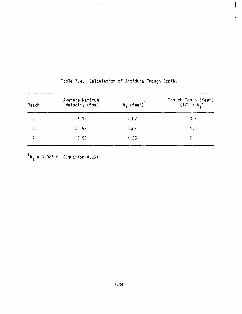
Table 7.4. Calculation of Antidune Trough Depths.
Reach
2
3
4
Average MaximumVelocity (fps)
16.18
17.92
12.56
ha (feet)1
7.07
8.67
4.26
Trough Depth(1/2 x h
3.5
4.3
2.1
(feet)
a)
1ha = 0.027 V2 (Equation 4.25)
7.34

2. Reach 2 - This reach will be armored along the east bank, as a resultof the proposed soil-cement levee, and presently consists of naturalrock along the west bank. As a result, no lateral channel movementis expected to occur in this reach.
3. Reach 3 - From the sediment continuity analysis, this reach has atotal sediment supply deficit of 686 cfs (see Table 7.2). This valueis converted to a volume as follows:
Vol. = AQS x At x 3,600 sec./hr.
Vol. = (686) (1 hour) (3,600)
Vol. = 2,469,600 feet3
Correct for bulking (assuming a porosity of n = 0.4),
Vol. = 2.469,600 = 4,116,000 feet3
The average west bank height (H) through Reach 3 is six feet, whilethe Dank length is 1,170 feet. Assuming uniform erosion, the lateralbank movement is computed as follows:
Volume Sed. Def
AW =
HWB x UB
4,116,000[6) (1,170)
AW = 586 feet
An alternative to the uniform erosion approach is to assume the ero-sion will occur as a semi -circular bend. The volume of erosion iscomputed as:
Vo1umeBank = " r H
Assuming the volume of bank erosion equals the volume of sedimentdeficit (i.e., bed and bank materials are similar); or
VolumeBank = Volume5ed_ Qef
we can solve for the radius of the semi-circle as follows:
'Vol ^ 1/2vo Sed. Ded.r -
7.35

[4,116,000 1LTSTUHH) J
r = 661 feet
The semi -circular erosion pattern gives a worst-case conch' tio_n forthis reach. Selection of the dimensions for an erosion buffer "zonealong the west bank is a matter of experience and engineering judge-ment, and should not be based solely on the results of a quantitativeanalysis such as that presented above. Cases may arise where itwould be more economical to construct some type of structural measureto prevent erosion, rather than purchasing the right-of-way for anerosion buffer zone.
For this project, an erosion buffer zone was selected as the pre-ferred alternative for the west bank. The west bank is undevelopedproperty and can be purchased at a low cost. Based on the results ofthe quantitative lateral migration analysis, a review of historicalphotos dating back to 1947, and the topography along the west bank, avariable width buffer zone was recommended for the west bank throughReach 3.
Due to the reconnaissance level nature of the Department of WaterResource study, subsurface geological data was not available for thestream bank opposite the proposed levee. However, a rock formationis visible along the west bank through the majority of Reach 2. Thetopography along the west bank suggests that this rock formation con-tinues under the surface and probably constitutes the steep ridgelinealong the west bank of Reach 3. On this assumption, the buffer zonefor Reach 3 will be taken as that area from the west edge of the100-year floodplain to the base of the steep ridge (see Figure 7.1).This width will vary from 200' to 300', and is within the limitsderived from the quantitative analysis. Obviously, the geologicalassumptions used in this analysis would have to be verified prior toa final delineation and acquisition of the buffer zone.
Reach 4 - The sediment continuity analysis indicates this reach willreceive more sediment than it is capable of transporting. As aresult, bank erosion due to insufficient sediment supply should notoccur. However, as the bed aggrades, the channel geometry couldchange and cause the main channel to shift westerly and possiblyattack the western bank with high velocity flow. This is a verydynamic process which is difficult to quantify. Estimating theamount of lateral erosion in aggrading reaches is a matter of engi-neering judgement. Again, as for Reach 3, topographic features andhistorical photos were used in establishing a realistic buffer zonethrough Reach 4. This zone is an extension of the one through Reach3 and essentially follows the base of another steep ridgeline whichis suspected to be overlying rock along the northern half of thereach (see Figure 7.1 for buffer zone limits).
7.36

r* Although Figure 7.1 does not extend far enough downstream to showthis feature, Pinto Creek makes about a 45° bend to the east afterleaving Reach 4. In the absence of any visible topographic or geolo-
!~ gic erosion resistant features in this downstream area, there is agood chance that some accelerated erosion could occur on the outsideof this bend. This erosion process may be further accelerated as aresult of the straightened alignment of the river from the Highway 88bridge through Reach 4. The proposed levee tends to concentrate theflood water in a straight line that is directed into this bend.Prior to construction of the proposed levee, the water spread outthrough Sportsman's Haven and did not launch such a concentratedattack at the entrance to the bend.
As part of the final design phase of this project, it would be recom-mended that a detailed analysis be made of this problem in order thatmitigation measures might be taken if the damage potential was foundto be severe and directly related to construction of the upstreamlevee system.
The quantitative assessment of lateral migration presented in this sec-tion is based on a single flood event. Realizing that lateral migration is a
continual process over a long period of time, some safety factor, say 2.0,
£ouj_d be applied to the quantitative calculations to establish a long-termlimit. It must be emphasized, however, that quantitative calculations should
only be used with considerable engineering judgement and an appreciation of
historical events and physical constraints such as topography and geology.
7• Summary and Conel_u_s_i_onsBased on the preceding analyses, we are now prepared to establish the
critical design dimensions for the proposed levee system.
1. Levee Crest Profi1eThe crest of theTTevee will parallel the subcritical water-surfaceprofile for the 100-year flood. As shown below, the top of thelevee embankment and the soil-cement bank protection will De elevatedan equal distance above this water-surface profile. These freeboarddimensions are minimum values and may be increased slightly duringdesign to eliminate numerous grade breaks during actual leveeconstruction.
7.37

Freeboard Distance Above Design WaterSurface Profile (feet)
Reach Levee Crest Soil-Cement Lining
UpstreamRight Overbank 3.0 3.0
2 3.8 3.83 4.2 4.24 3.1 3.1
2. Requirements For Bank StabilizationThe~~need for~barTk stabil izTtioTi to'prevent erosion of the earth leveewas discussed in Section 7.3.2.1. For this project, a soil-cementblanket is proposed along the stream-side face of the levee to pre-vent erosion.
3• Toe-Down Requirements For Soil-Cement EmbankmentThe soil cement must be extended far enough below existing groundelevation so as to prevent undermining by the multiple scouring pro-cesses that occur on both a short and long-term basis. This toe-downdimension is determined as the sum of all the vertical channeladjustments that were analyzed in Section 7.3.2.2. A summary of therecommended toe-down depths for specific reaches of the levee is pre-sented in Table 7.5.
4. Lateral Channel MigrationArmoring of the proposed east bank levee through an application ofsoil cement may accelerate erosion along the opposite bank of thestream. As a precautionary measure, an erosion buffer zone is recom-mended along the west bank of Pinto Creek. The buffer zone dimen-sions are summarized as follows:
Reach Buffer Zone (feet)
234
0 (natural200 - 300130 - 350
rock
For this project, the buffer zone will be measured from the west edgeof the 100-year flood plain. Unique circumstances on other projectsmight dictate that such buffer zones be measured from differentreference points.
7.38

Table 7.5. Summary of Soil-Cement Toe-Down Dimensions.
Total4
Long-Term Low Flow Local General Antidune CalculatedDegradation Incisement Scour Scour Troughs Safety Toe-Down
Reach (feet) (feet) (feet) (feet) (feet) Factor (feet)
UpstreamRightOverbank (H
UpstreamLeveeCorner (A
2 Ol
3 O1
4 Ql
N/A2
N/A2
N/A2
N/A2
N/A2
0
6.9
0
0
0
2.23 0
3.6 3.5
3.6 3.5
5.3 4.3
O1 2.1
1.3
1.3
1.3
1.3
1.3
2.9
18.2
9.2
12.5
2.7
•'-The equilibrium slope or general scour analysis predict aggradation or depo-sition, respectively, at these locations. As a conservative approach,aggradation or desposition is not algebraicly added into the toe-down depth,a zero bed adjustment is assumed for these cases.
2The invert of the existing low flow channel will be used as a base elevationfrom which all other bed profile adjustments will be measured.
3(3n the basis of engineering judgement, the hydraulic depth in the right over-bank was selected as being representative of this type of scour.
^These are minimum values and may be increased slightly during design to eli-minate numerous grade breaks during construction.
7.39

This concludes the design example. The intent of this section was to
illustrate the application of analytical concepts presented in this manual to
an actual project study. As can be seen from the above analysis, "real world"
problems do not always conform to the ideal conditions often used to describe
the theory of a technical procedure. For instance, in this problem we found
no controls in the channel bed that could be used as pivot points for an
equilibrium slope analysis. A problem was also suspected in the selection of
a sediment supply section for the equilibrium slope analysis. The lateralmigration analysis demonstrated the need for considerable engineering judge-
ment in selecting an erosion buffer zone.
Very seldom will projects involving fluvial systems be encountered that
lend themselves to an ideal or textbook solution. All the quantitative proce-
dures outlined in this manual should only be used as guidelines. As empha-
sized throughout this design manual, the final solution to a specific problemmust be based on engineering judgement and experience.
7.40

VIII. REFERENCES
Agricultural Research Service, 1979, Field Manual for Research in AgriculturalHydrology, Agricultural Handbook 224, February.
Anderson, A. G., A. S. Paintal, and J. T. Davenport, 1970, Tentative DesignProcedure for Riprap-Lined Channels; Project Report No. 96, St. Anthony FallsHydraulics Laboratory, Minneapolis, Minnesota, NCHRP Report 108, HighwayResearch Board, Washington, D.C.
ASCE Task Force Committee, 1963, Friction Factors in Open Channels, Journal ofthe Hydraulics Division, Proc. ASCE, Vol. 89, No. HY2, March.
Bathurst, J. C., 1978, Flow Resistance of Large-Scale Roughness, Journal ofthe Hydraulics Division, ASCE, Vol. 104, No. HY12, Proc. Paper 14239, pp.1587-1603.
Chow, V. T., 1959, Open-Channel Hydraulics, McGraw-Hill, New York, 680 pp.
Chow, V. T., 1962, Hydrologic Determination of Waterway Areas for the Designof Drainage Structures in Small Drainage Basins, University of IllinoisEngineering Experiment Station Bulletin No. 462, 104 pp, Urbana, Illinois.
Colby, B. R., 1964, Practical Computations of Bed-Material Discharge, Journalof the Hydraulics Division, ASCE, Vol. 90, No. HY2.
Colby, B. R., and C. H. Hembree, 1955, Computation of Total SedimentDischarge, Niobrara River Near Cody, Nebraska, U.S. Geological Survey WaterSupply Paper 1357.
Culvertson, D. M., L. E. Young, and J. C. Brice, 1967, Scour and F i l l inAl l u v i a l Channels: U.S. Geol. Surv. Open-File Report, 58 pp.
Denver Urban Drainage and Flood Control District, 1982, Urban Storm DrainageCriteria Manual, Volume 2, Section 5, Riprap (revised from 1969 version).
Einstein, H. A., 1950, The Bed Load Function for Sediment Transportation inOpen Channel Flows, U.S. Department of Agriculture, Soil Conservation Service,Technical Bulletin No. 1026.
Friedkin, J. F., 1945, A Laboratory Study of the Meandering of AlluvialChannels, U.S. Army Corps of Engineers, Waterways Experiment Station.
Gessler, J., 1971, Beginning and Ceasing of Sediment Motion, River Mechanics,Chapter 7, edited by H. W. Shen, Fort Collins, Colorado, 22 pp.
Green, W. H., and C. A. Ampt, 1911, Studies on Soil Physics, I, Flow of Airand Water Through Soils, Journal of Agricultural Science, Vol. 4, pp. 1-24.
Haan, C. T., 1977, Statistical Methods vn Hydrology, Iowa State UniversityPress, Ames, Iowa.
Henderson, F. M., 1966, Open Channel Flow, The McMillan Company, New York.
8.1

Hershfield, D. M., 1961, Rainfall Frequency Atlas of the United States, forDurations from 30 Minutes to 24 Hours and Return Periods from 1 to 100 Years,Technical Paper No. 40, United States Weather Bureau.
Ippen, A. T., and P. A. Drinker, 1962, Boundary Shear Stress in CurvedTrapezoidal Channels, Journal p_f_ the Hydraulics Division, ASCE, Vol. 88, No.HY5, September.
Kaan, H. R., 1971, Laboratory Study of River Morphology: unpublished Ph.D.Dissertation, Colorado State University, 189 pp.
Kellerhals, R., and D. I. Bray, 1971, Sampling Procedures for Coarse FluvialSediments, Journal of the Hydraulics Division, ASCE, Vol. 97, No. HY8, August.
Kennedy, J. F., 1963, The Mechanics of Dunes and Antidunes in Erodible-BedChannels, Journal of Fluid Mechanics, Vol. 16, pt. 4, pp. 521-544.
Kite, G. W., 1977, Frequency and Risk Analyses in Hydrology, Water ResourcesPublications, Fort Collins, Colorado.
Lagasse, P. F., J. D. Schall, and M. R. Peterson, 1984, Erosion Risk Analysisfor a Southwestern Arroyo, paper accepted for publication in the Journal ofUrban Planning and Development, ASCE.
Lane, E. W., 1955, The Importance of Fluvial Morphology in HydraulicEngineering: Am. Soc. Civil Eng. Proc., Vol. 81, No. 745, 17 pp.
Lane, E. W., 1957, A Study of the Shape of Channels Formed by Natural StreamsFlowing in Erodible Material," Missouri River Division Sediment Series No. 9,U.S. Army Engineer Division, Missouri River, Corps of Engineers, Omaha,Nebraska.
Lane, E. W. and E. J. Carlson, 1953, Some Factors Affecting the Stability ofCanals Constructed in Coarse Granular Materials, Proc. Minnesota InternationalHydraulics Convention, September.
Laursen, E. M., and A. Toch, 1956, Scour Around Bridge Piers and Abutments,Iowa Highway Research Board, Bulletin No. 4, May.
Leopold, L. B., W. W. Emmett, and R. M. Myrick, 1966, Channel and HillslopeProcesses in a Semiarid Area, New Mexico, U.S. Geological Survey ProfessionalPaper 352-G, U.S. Geological Survey, Washington, D.C.
Leopold, L. B., and M. G. Wolman, 1967, River Channel Patterns: Braided,Meandering, and Straight, USGS Prof. Paper 282-B, 85 pp.
Leopold, L. B., M. G. Wolman and J. P. Miller, 1964, Fluvial Processes ir\_Geomorphology, San Francisco: W. Freeman.
Li, R. M., and D. B. Simons, 1979, Failure Probability of Riprap Structures,paper presented to the ASCE Conference and Exposition, Atlanta, Georgia, Oct.23-25.
8.2

Li, R. M., M. A. Stevens and D. B. Simons, 1976, Solutions to the Green-AmptInfiltration Equation, Journal of the Irrigation and Drainage Division, ASCE,Vol. 102, No. IR2, Proc. Paper 12196, June.
McCuen, R. J., W. J. Rawls, G. T. Fisher and R. L. Powell, 1977, FloodFrequency Estimation at Ungaged Locations: State of the Art, Water Supply andManagement, Vol. 3, Pergamon Press, Ltd., Great Britain.
McPherson, M. B., 1969, Some Notes in the National Method of Storm DrainageDesign, Technical Memorandum No. 6, ASCE Urban Water Resources Program, ASCE.
Meyer-Peter, E., and R. Muller, 1948, Formulas for Bed Load Transport, Proc.,3rd Meeting of IAHR, Stockholm, pp. 39-64.
National Weather Service, 1977, Five to 60 Minute Precipitation Frequency forthe Eastern and Central United States (HYDRO-55).
Osterkamp, W. R., and E. R. Hedman, 1981, Perennial-Streamflow CharacteristicsRelated to Channel Geometry and Sediment in the Missouri River Basin, inpress, USGS Professional Paper.
Reich, B. M., 1960, Annotated Bibliography and Comments on the Estimation ofFlood Peaks from Small Watersheds, Technical Report CER60M452, 66 pp., CivilEngineering Department, Colorado State University, Fort Collins.
Reich, B. M., 1971, Ruonff Estimates for Small Rural Watersheds, 136 pp.,Civil Engineering Department, The Pennsylvania State University, UniversityPark.
Renard, K. G., 1980, Estimating Erosion and Sediment Yield from Rangelands,Proceedings ASCE Symposium on Watershed Management, pp. 164-175.
Richardson, E. V., D. B. Simons, S. Karaki, K. Mahmood, and M. A. Stevens,1975, Highways in the River Environment, Hydraulic and Environmental DesignConsiderations, Training and Design Manual prepared for U.S. Department ofTransportation, Federal Highway Administration, May.
Roeske, R. H., 1978, Methods for Estimating the Magnitude and Frequency ofFloods in Arizona, Arizona Department of Transportation, RS-15(121).
Rozovskii, I. L., 1961, Flow of Water in Bends of Open Channels, IsraelProgram for Scientific Translations, Jerusaleum, Israel.
Schumm, S. A., 1977, Jhe Fluvial System, John Wiley and Sons, Inc., New York.
Schwab, G. 0., R. K. Frevert, T. W. Edminster, and K. K. Barnes, 1966, Soiland Water Consen/ation Engineering, John Wiley and Sons, Inc., New York.
Shen, H. W., 1971, Wash Load and Bed Load, _Rjj/er Mechanics, H. W. Shen, ed.,Water Resources Publications, Fort Collins, Colorado, 30 pp.
8.3

Shields, A., 1936, Anwendung der Ahnlichkeltschechanik und Turbulenz Forschungauf die Geschiebebewegung, Metteil. Preuss. Versuchsanst. Wasser, Erd.Schiffsbau, Berlin, No. 26.
Shov/n, L. M., 1970, Evaluation of a Method for Estimating Sediment Yield, U.S.Geological Survey Professional Paper 700-B, U.S. Geological Survey,Washington, D.C., pp. 245-249.
Simons, D. B., Y. H. Chen, and L. J. Swenson, 1983, Hydraulic Test to DevelopDesign Criteria for the Use of Reno Mattresses, report prepared for MaccaferriSteel Wire Products, Ltd., Ontario, Canada.
Simons, D. B., R. M. Li and W. T. Fullerton, 1981, Theoretically DerivedSediment Transport Equations for Pima County, Arizona, Simons, Li &Associates, Inc., Fort Collins, Colorado, prepared for Pima Coiunty DOT andFlood Control District, Tucson, Arizona.
Simons, D. B., and E. V. Richardson, 1960, Resistance to Flow in AlluvialChannels. Journal of the Hydraulics Division, ASCE, Vol. 86, No. HY5, May.
Simons, D. B., and E. V. Richardson, 1966, Resistance to Flow in AlluvialChannels, U.S. Geological Survey Professional Paper 422-J.
Simons, D. B., and F. Senturk, 1977, jd_i_mejrt Transport Technology, WaterResources Publications, Fort Collins, CoToTado"
Simons, Li & Associates, Inc., 1982, Engineering Analysis of Fluvial Systems,published by Simons, Li & Associates, ~prT"nted and "bound by BookCrafterT,~IrFcT,Chelsea, Michigan.
Soil Conservation Service, 1976 (TR55)
Soil Conservation Service, 1977, Design of Open Channels, Technical ReleaseNo. 25, October.
U.S. Army Corps of Engineers, 1970, Hydraulic Design of Flood ControlChannels, Engineer Manual EM 1110-2-1601, July.
U.S. Army Corps of Engineers, 1970, J jrato_ry_ _Soj_l_s Testing, EM 1110-2-1906,November.
U.S. Bureau of Reclamation, 1960, Investigation of Meyer-Peter, Muller BedloadFormulas: Sedimentation Section, Hydrology Branch, Division of ProjectInvestigations, Denver, Colorado.
U.S. Bureau of Reclamation, 1977, Design of jmal1 Dams.
U.S. Bureau of Reclamation, 1984, Computing Degradation and Local Scour,Technical Guideline for Bureau of Reclamation, prepared by E. L. Pemberton andJ. M. Lara, January.
8.4

U.S. Geological Survey, 1969, Laboratory Theory and Methods for SedimentAnalysis, TWRI, Book 5, Ch. Cl.
Viessmann, W., T. E. Harbaugh and J. W. Knapp, 1972, Introduction _to_Hydro1qgy, Intext Educational Publishers, New York. ~~
Williams, J. R., and H. D. Berndt, 1972, Sediment Yield Computed withUniversal Equation, Journal erf the jjyjd _]_lcs Division, ASCE, Vol. 98, No.HY12, Proc. Paper 942lT7~December, pp. 2087-2097.
Wischmeier, W. H., and D. D. Smith, 1978, Predicting Rainfall Erosion Losses,Agricultural Handbook 537, Science and Education Administration, USDA.
Yevjevich, V., 1972, Probability and Statistics in Hydrology, Water ResourcesPublications, Fort Collins, Colorado.
Zeller, M. E., and W. T. Fullerton, 1983, A Theoretically Derived SedimentTransport Equation for Sand-Bed Channels in Arid Regions, Proc. of the D. B.Simons Symposium on Erosion and Sedimentation, R. M. Li and P. F. Lagasse,eds.
Zeller, M. E., 1981, Scour Depth Formula for Estimation of Toe ProtectionAgainst General Scour, Pi ma County Department of Transportation and FloodControl District, Tucson, Arizona.
8.5

APPENDIX A
PACIFIC SOUTHWEST INTER-AGENCY COMMITTEE (PSIAC)
METHOD FOR PREDICTING WATERSHED SOIL LOSS
Note: The information presented in APPENDIX A is from the following source:
"Pacific Southwest Inter-Agency Committee, Report of the WaterManagement Subcommittee on Factors Affecting Sediment Yield in the
Pacific Southwest Area and Selection and Evaluation of Measures for
Reduction of Erosion and Sediment Yield," October, 1968.
Introduction
The material that follows is suggested for use in the evaluation of sedi-
ment yield in the Pacific Southwest. It is intended as an aid to the estima-
tion of sediment yield for the variety of conditions encountered in this area.The classifications and companion guide material are intended for broad
planning purposes only, rather than for specific projects where more intensive
investigations of sediment yield would be required. For these purposes it is
recommended that map delineations be for areas no smaller than 10 square
miles.
It is suggested that actual measurements of sediment yield be used to thefullest extent possible. This descriptive material and the related numerical
evaluation system would best serve its purpose as a means of delineating boun-
daries between sediment yield areas and in extrapolation of existing data to
areas where none is available.This may involve a plotting of known sediment yield data on work maps.
Prepared materials such as geologic and soil maps, topographic, climatic,vegetative type and other references would be used as aids in delineation of
boundaries separating yield classifications. A study of the general rela-tionships between known sediment yield rates and the watershed conditions that
produce them would be of substantial benefit in projecting data to areaswithout information.
A.I

Sediment Y je ldC las sification
It is recommended that sediment yields in the Pacific Southwest area be
divided into f ive classes of average annual yield in acre-feet per square
mile. These are as fol lows:
Classif icat ion 1 > 3.0 acre-feet/square mile
2 1.0 - 3.0
3 0.5 - 1.0
4 0.2 - 0.5
5 < 0.2
Nine factors are recommended for consideration in determining the sedi-
ment yield classif ication. These are geology, soils, climate, runoff,
topography, ground cover, land use, upland erosion, and channel erosion and
sediment transport.
Characteristics of each of the nine factors which give that factor high,
moderate, or low sediment yield level are shown on Table A-l. The sediment
yield characteristic of each factor is assigned a numerical value representing
its relative significance in the yield rating. The yield rating is the sum of
values for the appropriate characteristics for each of the nine factors.
Conversion to yield c lasses should be as fol lows:
Rating C lass
> 100 1
75 - 100 2
5 0 - 7 5 3
2 5 - 5 0 4
0 - 2 5 5
Guidelines which accompany the table are an integral part of the proce-
dure. They describe the characterist ics of factors which influence sediment
yield and these are summarized in the space provided on the table.
The factors are generally described, for purposes of avoiding complexity,
as independently influencing the amount of sediment yield. The variable impact
of any one factor is the result of influence by the others. To account for
this variable influence in any one area would require much more intensive
investigational procedures than are avai lable for broad planning purposes.
A.2

To briefly indicate the interdependence of the factors discussed separa-tely, ground cover is used as an example. If there is no vegetation, litter
or rock fragments protecting the surface, the rock, soil, and topography
express their uniqueness on erosion and sediment yield. If the surface is
very well protected by cover, the characteristics of the other factors are
obscured by this circumstance. In similar vein, an arid region has a high
potential for erosion and sediment yield because of little or no ground cover,
sensitive soils and rugged topography. Given very low intensity rainfall and
rare intervals of runoff, the sediment yield could be quite low.
Each of the 9 factors shown on Table A-l are paired influences with theexception of topography. That is, geology and soils are directly related as
are climate and runoff, ground cover and land use, and upland and channel ero-
sion. Ground cover and land use have a negative influence under average or
better conditions. Their impact on sediment yield is therefore indicated as a
negative influence when affording better protection than this average.
It is recommended that the observer follow a feedback process whereby he
checks the sum of the values on the table from A through G with the sum ofand I. In most instances high values in the former should correspond to hie
values in the latter. If they do not, either special erosion conditions existor the A through G factors should be re-evaluated.
Although only the high, moderate and low sediment yield levels are shownon the attached table, interpolation between these levels may be made.
Surface Geology
Over much of the southwest area, the effect of surface geology on erosionis readily apparent. The weaker and softer rocks are more easily eroded and
generally yield more sediment than do the harder more resistant types.
Sandstones and similar coarse-textured rocks that disintegrate to form per-
meable soils erode less than shales and related mudstones and siltstones underthe same conditions of precipitation. On the other hand, because of the
absence of cementing agents in some soils derived from sandstone, large stormsmay produce some of the highest sediment yields known.
The widely distributed marine shales, such as the Mancos and shale mem-bers of the Moenkopi Formation, constitute a group of highly erodible for-
mations. The very large area! extent of the shales and their outwash deposits
A.3

gives them a rank of special importance in relation to erosion. Few of the
shale areas are free from erosion. Occasionally, because of slope or cover
conditions, metamorphic rocks and highly fractured and deeply weathered grani-
tes and granodiorites produce high sediment yield. Limestone and volcanic
outcrop areas are among the most stable found within the western lands. The
principal reason for this appears to be the excellent infiltration charac-
teristics, which allow most precipitation to percolate into the underlying
rocks.In some areas, all geologic formations are covered with alluvial or
colluvial material which may have no relation to the underlying geology. In
such areas the geologic factor would have no influence and should be assigned
a value of 0 in the rating.
Soil s
Soil formation in the Pacific Southwest generally has not had climatic
conditions conducive to rapid development. Therefore, the soils are in an
immature stage of development and consist essentially of physically weatheredrock materials. The presence of sodium carbonate (black alkali) in a soil
tends to cause the soil particles to disperse and renders such a soil suscep-tible to erosion.
There are essentially three inorganic properties—sand, silt, and clay—
which may in any combination give soil its physical characteristics. Organic
substances plus clay provide the binding material which tends to hold the soil
separates together and form aggregates. Aggregate formation and stability of
these aggregates are the resistant properties of soil against erosion.
Unstable aggregates or single grain soil materials can be very erodible.
Climate and l i v i n g organisms acting on parent material, as conditioned by
relief or topography over a period of time, are the essential factors for soil
development. Any one of these factors may overshadow or depress another in a
given area and cause a difference in soil formation. For instance, climate
determines what type of vegetation and animal population will be present in an
area, and this will have a definite influence or determine the type of soil
that evolves. As an example, soils developing under a forest canopy are muchdifferent from soils developing in a grassland community.
The raw, shaley type areas (marine shales) of the Pacific Southwest have
very little, if any, solid development. Colluvial-alluvial fan type areas are
A.4

usually present at the lower extremities of the steeper sloping shale areas.Infiltration and percolation are usually minimal on these areas due to thefine textured nature of the soil material. This material is easily dispersedand probably has a high shrink-swell capacity. Vegetation is generally
sparse, and consists of a salt desert shrub type.There are areas that contain soils with definite profile development, and
also, stony soils that contain few fines, which constitutes an improved physi-cal condition for infiltration and plant growth over the fine textured shaleyareas. These areas usually occur at higher and more moist elevations wherebare, hard crystalline rocks provide the soil parent material. Vegetation andother ground cover, under these circumstances, provide adequate protectionagainst the erosive forces and thus low sediment yield results.
In arid and semi-arid areas, an accumulation of rock fragments (desertpavement) or calcareous material (caliche) is not uncommon. These layers canoffer substantial resistance to erosion processes.
The two extreme conditions of sediment yield areas have been described.Intermediate situations would contain some features of the two extremes. Onesuch situation might be an area of predominately good soil development thatcontains small areas of badlands. This combination would possibly result inan intermediate classification.
Climate and Runoff
Climatic factors are paramount in soil and vegetal development and deter-mine the quantity and discharge rate of runoff. The same factors constitutethe forces that cause erosion and the resultant sediment yield. Likewise,temperature, precipitation, and particularly the distribution of precipitationduring the growing season, affect the quantity and quality of the groundcover as well as soil development. The quantity and intensity of precipita-
tion determine the amount and discharge rates of runoff and resultant detach-ment of soil and the transport media for sediment yield. The intensity ofprevailing and seasonal winds affects precipitation pattern, snow accumulationand evaporation rate.
Snow appears to have a minor effect on upland slope erosion sinceraindrop impact is absent and runoff associated with snow melt is generally inresistant mountain systems.
A.5

Frontal storms in which periods of moderate to high intensity precipita-
tion occur can produce the highest sediment yields within the Southwest. In
humid and subhumid areas the impact of frontal storms on sediment may be
greatest on upland slopes and unstable geologic areas where slides and other
downhill soil movement can readily occur.
Convective thunderstorm activity in the Southwest has its greatest
influence on eroison and sedimentation in Arizona and New Mexico and portions
of the adjoining states. High rainfall intensities on low density cover or
easily dispersed soils produces high sediment yields. The average annual
sediment yield is usually kept within moderate bounds by infrequent occurrence
of thunderstorms in any one locality.
High runoff of rare frequency may cause an impact on average annual sedi-
ment yield for a long period of time in a watershed that is sensitive to ero-
sion, or it may have little effect in an insensitive watershed. For example,
sediment that has been collecting in the bottom of a canyon and on side slopes
for many years of low and moderate flows may be swept out during the rare
event, creating a large change in the indicated sediment yield rate for the
period of record.
In some areas the action of freezing and thawing becomes important in theerosion process. Impermeable ice usually forms in areas of fine textured
soils where a supply of moisture is a v a i l a b l e before the advent of coldweather. Under these conditions the ice often persists throughout the winterand is still present when the spring thaw occurs. In some instances water
tends to run over the surface of the ice ana not aetacn soil particles, but it
is possible for the ice in a surface layer to thaw during a warm period and
create a very erodible situation. Spring rains with ice at shallow depth maywash away the loose material on the surface.
In some areas of the Pacific Southwest, particularly those underlain by
marine shale, freezing and thawing alters the texture of soil near the sur-
face, and thus changes the infiltration characteristics. These areas
generally do not receive enough snow or have cold enough temperatures to build
a snow pack for spring melt. Later in the year soil in a loosened condition isable to absorb a large part of the early rainfall. As rains occur during the
summer, the soil becomes compacted on the surface, thus allowing more water to
run off and affording a greater chance for erosion.
A.6

Topography
Watershed slopes, relief, floodplain development, drainage patterns,
orientation and size are basic items to consider in connection with
topography. However, their influence is closely associated with geology,
soils, and cover.Generally, steep slopes result in rapid runoff. The rimrock and
badlands, common in portions of the Pacific Southwest, consist of steep slopes
of soft shales usually maintained by the presence of overlying cap rock. As
the soft material is eroded, the cap rock is undercut and falls, exposing moresoft shales to be carried away in a continuing process. However, high sedi-
ment yields from these areas are often modified by the temporary deposition of
sediment on the intermediate floodplains.
The high mountain ranges, although having steep slopes, produce varying
quantities of sediment depending upon the type of parent materials, soil deve-
lopment, and cover which directly affect the erosion processes.
Southerly exposed slopes generally erode more rapidly than do the
northerly exposed slopes due to greater fluctuation of air and soil tem-
peratures, more frequent freezing and thawing cycles, and usually less ground
cover.
The size of the watershed may or may not materially affect the sediment
yield per unit area. Generally, the sediment yield is inversely related to
the watershed size because the larger areas usually have less overall slope,smaller proportions of upland sediment sources, and more opportunity for thedeposition of upstream derived sediments on floodplains and fans. In addi-
tion, large watersheds are less affected by small convective type storms.However, under other conditions, the sediment yield may not decrease as the
watershed size increases. There is little change in mountainous areas of
relatively uniform terrain. There may be an increase of sediment yield as the
watershed size increases if downstream watersheds or channels are more suscep-
tible to erosion than upstream areas.
Ground Cover
Ground cover is described as anything on or above the surface of the
ground which alters the effect of precipitation on the soil surface and pro-
file. Included in this factor are vegetation, litter, and rock fragments. A
A.7

good ground cover dissipates the energy of rainfall before it strikes the
soil surface, delivers water to the soil at a relatively uniform rate, impedes
the flow of water, and promotes infiltration by the action of roots within the
soil. Conversely, the absence of ground cover, whether through natural growth
habits or the effect of overgrazing or fire, leave the land surface open to the
worst effects of storms.In certain areas, small rocks or rock fragments may be so numerous on the
surface of the ground that they afford excellent protection for any underlying
fine material. These rocks absorb the energy of falling rain and areresistant enough to prevent cutting by flowing water.
The Pacific Southwest is made up of land with all classes of ground
cover. The high mountain areas generally have the most vegetation, while many
areas in the desert regions have practically none. The abundance of vegeta-
tion is related in a large degree to precipitation. If vegetative ground
cover is destroyed in areas where precipitation is high, abnormally high ero-
sion rates may be experienced.
Differences in vegetative type have a variable effect on erosion and
sediment yield, even though percentages of total ground cover may be the same.
For instance, in areas of pinyon-juniper forest having the same percentage of
ground cover as an area of grass, the absence of understory in some of the
pinyon-juniper stands would allow a higher erosion rate than in the area ofgrass.
Land Use
The use of land has a widely variable impact on sediment yield, depending
largely on the susceptibility of the soil and rock to erosion, the amount ofstress exerted by climatic factors and the type and intensity of use. Factors
other than the latter have been discussed in appropriate places in this guide.
In almost all instances, use either removes or reduces the amount of
natural vegetative cover which reflects the varied relationships within the
environment. Activities which remove all vegetation for parts of each year
for several years, or permanently, are cultivation, urban development, and
road construction. Grazing, logging, mining, and fires artifically inducepermanent or temporary reduction in cover density.
High erosion hazard sites, because of the geology, soils, climate, etc.,
are also of high hazard from the standpoint of type and intensity of use. For
A.8

example, any use which reduces cover density on a steep slope with erodible
soils and severe climatic conditions will strongly affect sediment yield. The
extent of this effect will depend on the area and intensity of use relative to
the availability of sediment from other causes. Construction of road or urban
development with numerous cut and fill slopes through a large area of
widespread sheet or gully erosion will probably not cause a change in sediment
yield classification. Similar contruction and continued disturbance in an
area of good vegetative response to a favorable climate can raise yield by one
or more classifications.
Use of the land has its greatest potential impact on sediment yield wherea delicate balance exists under natural conditions. Alluvial valleys of fine,
easily dispersed soils from shales and sandstones are highly vulnerable to
erosion where intensive grazing and trailing by livestock have occurred.
Valley trenching has developed in many of these valleys and provides a large
part of the sediment in high yield classes from these areas.A decline in vegetative density is not the only effect of livestock on
erosion and sediment yield. Studies at Badger Wash, Colorado, which is
underlain by fiances shale, have indicated that sediment yield from ungrazed
watersheds is appreciably less than from those that are grazed. This dif-
ference is attributed to the absence of soil trampling in the ungrazed areas,
since the density of vegetation has not noticeably changed since exclusionbegan.
Areas in the arid and semi-arid portions of the Southwest that are sur-faced by desert pavement are much less sensitive to grazing and other use,
since the pavement affords a substitute for vegetative cover.
In certain instances the loss or deterioration of vegetative cover may
have little noticeable on-site impact but may increase off-site erosion by
acceleration of runoff. This could be particularly evident below urbanized
areas where accelerated runoff from pavement and rooftops has increased the
stress on downstream channels. Widespread destruction of cover by poor
logging practices or by brush and timber fires frequently increases channelerosion as well as that on the directly affected watershed slopes. On the
other hand, cover disturbances under favorable conditions, such as a cool,
moist climate, frequently result in a healing of erosion sources within a few
years.
A.9

Upland SI ope Erosion
This erosion form occurs on sloping watershed lands beyond the confines
of valleys. Sheet erosion, which involves the removal of a thin layer of soil
over an extensive area, is usually not visible to the eye. This erosion form
is evidenced by the formation of rills. Experience indicates that soil loss
from rill erosion can be seen if it amounts to about 5 tons or more per acre.
This is equivalent in volume per square mile to aproximately 2 acre-feet.
Wind erosion from upland slopes and the deposition of the eroded materialin stream channels may be a significant factor. The material so deposited inchannels is readily moved by subsequent runoff.
Downs!ope soil movement due to creep can be an important factor in sedi-
ment yield on steep slopes underlain by unstable geologic formations.Significant gully erosion as a sediment contributor is evidenced by the
presence of numerous raw cuts along the hill slopes. Deep soils on moderately
steep to steep slopes usually provide an environment for gully development.
Processes of slope erosion must be considered in the light of factors
which contribute to its development. These have been discussed in previoussections.
Channel Erosion and _Sediment Transpo_rt
If a stream is ephemeral, runoff that traverses the dry alluvial bed may
be drastically reduced by transmission losses (absorption by channel
alluvium). This decrease in the volume of flow results in a decreased poten-
tial to move sediment. Sediment may be deposited in the streambed from one ora series of relatively small flows only to be picked up and moved on in a sub-
sequent larger flow. Sediment concentrations, determined from field measure-
ments at consecutive stations, have generally been shown to increase many fold
for instances of no tributary inflow. Thus, although water yield per unit
area will decrease with increasing drainage area, the sediment yield per unit
area may remain nearly constant or may even increase with increasing drainagearea.
In instances of convective precipitation in a watershed with perennial
flow, the role of transmission losses is not as significant as in watersheds
with ephemeral flow, but other channel factors, such as the shape of the chan-nel, may be important.
A.10

For frontal storm runoff, the flow durations are generally much longer
than for convective storms, and runoff is often generated from the entire
basin. In such instances, sediment removed from the land surfaces is
generally carried out of the area by the runoff. Stream channel degradation
and/or aggradation must be considered in such cases, as well as bank scour.
Because many of the stream beds in the Pacific Southwest are composed of fine-
grained alluvium in well defined channels, the potential for sediment
transport is limited only by the amount and duration of runoff. Large volumes
of sediment may thus be moved by these frontal storms because of the longer
flow durations.The combination of frontal storms of long duration with high intensity
and limited areal-extent convective activity will generally be in the highest
class for sediment movement in the channels. Storms of this type generally
produce both the high peak flows and the long durations necessary for maximum
sediment transport.
Sediment yield may be substantially affected by the degree of channeldevelopment in a watershed. This development can be described by the channel
cross sections, as well as by geomorphic parameters such as drainage density,
channel gradients and width-depth ratio. The effect of these geomorphic para-meters is difficult to evaluate, primarily because of the scarcity of sediment
transport data in the Pacific Southwest.
If the cross section of a stream is such as to keep the flow within
defined banks, then the sediment from an upstream point is generally
transported to a downstream point without significant losses. Confinement of
the flow within alluvial banks can result in a high erosional capability of a
flood flow, especially the flows with long return periods. In most channels
with wide floodplains, deposition on the floodplain during floods is often
significant, and the transport is thus less than that for a within bank flow.
The effect of this transport capability can be explained in terms of tractive
force which signifies the hydraulic stress exerted by the flow on the bed of
the stream. This average bed-shear stress is obtained as the product of the
specific weight of the fluid, hydraulic radius, and energy gradient slope.Thus, greater depth results in a greater bed shear and a greater potential for
moving sediment. By the same reasoning, steep slopes (the energy slope and
bed slope are assumed to be equivalent) also result in high bed-shear stress.
The boundary between sediment yield classifications in much of the
Pacific Southwest may be at the mountain front, with the highest yieldA • i i

designation on the alluvial plain if there is extensive channel erosion. In
contrast, many mountain streams emerge from canyon reaches and then spreadover fans or valley flats. Here water depths can decrease from many feet to
only a few inches in short distances with a resultant loss of the capacity to
transport sediment. Sediment yield of the highest classification can thus
drop to the lowest in such a transition from a confined channel to one thathas no definition.
Channel bank and bed composition may greatly influence the sediment yield
of a watershed. In many areas within the Pacific Southwest, the channels in
valleys dissect unconsolidated material which may contribute significantly tothe stream sediment load. Bank sloughing during periods of flow, as well as
during dry periods, piping, and bank scour generally add greatly to the sedi-
ment load of the stream and often change upward the sediment yield classifica-
tion of the watershed. Field examination for areas of head cutting,
aggradation or degradation, and bank cutting are generally necessary prior to
classification of the transport expectancy of a stream. Geology plays a
significant role in such an evaluation. Geologic controls in channels can
greatly affect the stream regimen by limiting degradation and headcuts. Thus,
the transport capacity may be present, but the supply of sediment from thissource is limited.
Man-made structures can also greatly affect the transport characteristics
of the stream. For example, channel straightening can temporarily upset the
channel equilibrium and cause an increase in channel gradient and an increase
in the stream velocity and the shear stress. Thus, the sediment transport
capacity of the stream may be temporarily increased. Structures such as
debris dams, lined channels, drop spillways, and detention dams may drasti-cally reduce the sediment transport.
A.12

AN EXPLANATION OF THE USE OF THE RATING CHART (TABLE A-l) FOR
EVALUATING FACTORS AFFECTING SEDIMENT YIELD IN THE PACIFIC SOUTHWEST FOLLOWS
A.13

Table A.I. Factors Affecting Sediment Yield in the Pacific Southwest.
Sediment Y i e l dLeve l s
High
<» *
Moderate
**
to.
ASURFACE GEOLOGT
MO)'
Stones •
< } )a. Rocks o medi urn
hard . sb. MoJ, at Iy
•eat er ac. Mode at Iy
f rac ur d
(0)
format ions
BSOILS
(10)
high s f r |nk-s*ti l 1
b. S i ng l e g» al n sf Itsand l ine sonds
15)a. Medium textured
b- Occa*.. lo^ai rockfragments
C. Col fche layers
C O )
b. Aggregated cf a y sc - Hi gfi In organ !c
matter
CCUMA7E
1 10)
days' durot Ion
of Intense rain-
fa. Frequ«nt Intenseconvect 1 *e storms
r. Fffx^e-tha*
(51o. S torrns of modor-
eto durat Ion andIntensi ty
vect Ive Storms
0)
in ens yb. Pr clp af lon In
(o « o S"O"c • Ar d c mate, low
d • Ar d c mote, rare
DRUNOFF
(10 )
per un 1 t area
f lo» per unit
(5 )a. Moderate peak
f lo-sb. Mod-rate voturw*
of t lo« per unl tarea
(0)
per unit areab. Lo* volufoo of
runof f per unf tares
c. Rare runoff
ETOPOGRAPHY
( 203
(In excess o' ?OI )
or no f loo'lp la in
(10)B. Moderate upland
Slopes ( le .s than20J)
b. Moderate fan orl loodplafn develop-ment
(0)
slopos f less than5JJ
b. Extens f vg el !uv!sipialns
FGROUND COVtR
(10 )
nut uxcood 2UJ
l i t t l e or no 111 tcr
sol I
•
(10)
Ing 401a- Not Iceab le M tterb. 1 f trees present
unde rs tory notwe! ! doveiopod
(-10)
protttcted by veg-et at Ion, rockfragment s, M tter.LHtie opportunity
material
GLAND USE
no)cu t t 1 vatod
area ! ntens I vol y
C. A l t o f areare-
(0)
cult 1 vattrf0. 50X or less re-
cent I y loggedc. less Ihon 50X fn-
tens i vel y graced
ott>er cons tructof
-10)
b. Ho re ent logglncC- Lov 1 terts 1 ty
groz 1 g
HUPLAND £ SOS ION
(?»
and gu 1 Iy cf
(10)a. About 25! of the
1 led by rill andgu My or Und-sMde erosion
b. Vin<3 erosion «lth
str «am channol s
(0)
of erosion
CHJNMfL FKQSI tXJ &S L L t t M E N T TNA.'-'.POftl
(A )
t f n u o u s l y or at
w i t h large depths and
b. A c t i v e headcuti. «nd
(10)
iw-dfgm f io« duration»l th occoslonfll Iyeroding tanks or bed
(Oi
w i t h f! t gradients,short ( o* durst Ion
b. Chenn«f In massiverock, i rge boui<ter$or B«I | veg-jloted
Channel
TOE NUHltRS IN SPECIFIC BOXES INDICATE VALUES TO BE ASSIGNED APPROPRIATE CHARACTERISTICS.THE SMALL LIITERS, o, b, c. RtFER TO INDEPENDENT CHARACTER S T I C S TO WHICH FULL VALUE WT EC ASSIGNED.
IF EXPERIENCE SO IND ICATES. INTERPOLATION BETWEEN THE 3 SEOI>CNT Tl tLO LEVELS HAT EC WOE.

Use of the Rating Chart of Factors AffectingSediment Yield in the Pacific Southwest
The following is a summary of the sediment yield classification presentedfor this methodology.
Sediment YieldClassification Rating _AF/sq. mi.
1 > 100 3.02 75 - 100 . 1.0 - 3.03 50-75 0.5 - 1.04 25-50 0.2 - 0.55 0-25 < 0.2
In most instances, high values for the A through G factors shouldcorrespond to high values for the H and/or I factors.
An example of the use of the rating chart is as follows:
A watershed of 15 square miles in western Colorado has the followingcharacteristics and sediment yield levels:
Factors Sediment Yield Levels Rating
A Surface geology Marine Shales 10B Soils Easily dispersed, high
shrink-swell characteristics 10C Climate Infrequent convective
storms, freeze-thaw occurrence 7D Runoff High peak flows; low volumes 5E Topography Moderate slopes 10F Ground cover Sparse, little or no litter 10G Land use Intensively grazed 10H Upland erosion More than 50% rill and gully
erosion 25I Channel erosion Occasionally eroding banks and
bed but short flow duration _5_
TOTAL 92
T h i s total ra t ing of 92 w o u l d i nd i ca t e that the sediment y i e ld is inC l a s s i f i c a t i o n 2. This compares wi th a sediment y i e ld of 1.96 acre-feet persquare m i l e as the average of a number of measurements in this area.
A.15

APPENDIX B
MODIFIED UNIVERSAL SOIL LOSS EQUATION
FOR PREDICTING WATERSHED SOIL LOSS
The Modified Universal Soil Loss Equation (MUSLE) described by Wil l iams
(1975) is an empirically derived methodology for predicting watershed sediment
yield on a per-storm basis. The MUSLE is
Y = R K L S C P (B.I)s w
where Y is sediment yield in tons for the storm event, R is a stormS W
runoff energy factor, K is the soil credibility factor, LS is the topo-
graphic factor representing the combination of slope length and slope gra-dient, C is th ecover and management factor and P is the erosion control
practice factor. Factors K, LS, C and P are as defined for the Uni-
versal Soil Loss Equation (USLE), as reviewed in later paragraphs (Smith and
Wischmeier, 1975, Wischmeier, 1960, and Wischmeier and Smith, 1978, provide
detailed descriptions of the USLE factors and their values).
The storm runoff energy factor R in Equation B.I represents the modi-
fication of the USLE where R is given byW
Rw = a (Vqp)a (B.2)
In Equation B.2, V is the storm event runoff volume in acre-feet, qp isthe storm event peak flow rate in cfs, and a and 3 are coefficients.
Utilization of a storm runoff factor makes the MUSLE applicable to semiarid
regions of the West where short-duration, high-intensity storms are cominant.
For watersheds having measured sediment data, values for the coefficients aand 3 can be derived through call oration. Williams and Berndt (1972) deter-
mined values for a and 3 of 95 and 0.56, respectively, for experimental
watersheds in Texas and Nebraska.
Soil credibility factor K was found by Wischmeier et al. (1971) to be a
function of percent of silt, percent of coarse sand, soil structure, per-
meability of soil, and percent of organic matter. The soil credibilitynomograph is shown in Figure B.I.
Wischmeier (1972) presented a method including graphical aids for deter-
mining the cover and management factor (cropping-management factor C). The
B.I

100 V
Figure B.I. Soil erodibility nomograph used to deter-mine factor K for specific topsoils orsubsoil horizons. Solutions are in tons/acre (from Wischmeier et al., 1971).
B.2

cropping-management factor can be divided into three distinct types of effects
as fol lows: Type I -effects of canopy cover (CJ, Type II - effects of mulch
or close-growing vegetation in direct contact with the soil surface (C,,) , and
Type III - tillage and residual effects of the land use ( C T T T ) - The cover and
management factor is defined as the product of these factors:
C = C I C n C I I I ( B . 3 )
Type I - Canopy Cover. Leaves and branches that do not directly contactthe soil are effective only as canopy cover. A canopy can intercept fallingraindrops, but waterdrops falling from the canopy may regain an appreciablevelocity, although not the terminal velocities of free-fall ing raindrops.
Therefore, canopy cover reduces rainfall erosivity by reducing impact energy
at the soil surface. The amount of reduction depends on height and density ofthe canopy. Figure B.2 shows the canopy factor as a function of height and
density of the canopy. Canopy factors for various percentages of cover at
heights of 0.5, 1.0, 2.0 and 4.0 meters may be obtained directly from thisgraph.
Type II - Mulch and Close-Growing Vegetation. A mulch at the soil-
atmosphere interface is much more effective than an equivalent percentage of
canopy cover. Because intercepted raindrops have no remaining fall-height tothe ground, their impact on the soil surface is eliminated. A mulch that
makes a good contact with the ground also reduces runoff velocity, which
greatly reduces the potential of runoff to detach and transport soil material.
Substantial rainfall simulator data are now available on erosion-reducing
effectiveness of various amounts and types of mulches used on cropland andconstruction sites. Extrapolation of these data to other mulches and close
covers such as those associated with range or woodland is facilitated by
expressing them on the basis of percent surface cover rather than tons peracre. This conversion and a preliminary summarization of data are reflected
in the relationship curve shown in Figure B.3.
Type III - Residua1_ Effects of _Lan_d__Use. This category includes residualeffects of land use on soil structure, organic matter content and soil den-
sity, effects of tillage or lack of tillage on surface roughness and porosity,
roots and subsurface stems, biological effects, and other factors. This fac-
tor can be evaluated from Figure B.4 by knowing the percent of root network in
the topsoil relative to a good rotation meadow. This percent of root network
B.3

1.00
0.80
u
?0.60
u8
0.40
0.20Foil Hei
. of Drop* From Conooy -
0.5m
20 «O 6O 6O IOO
Percent Ground Cov«r bv Conoov
Figure B.2. Influence of vegetal canopy on effective-El (after Wischmeier, 1972).
B.4

r
I 00
0 80
'0 60
0 00
0.20
20 «0 6O 80 100
ot So<l StXtoct Co»«r«d by MulCfi
Figure B.3. Effect of plant residues or close-growingstems at the soil surface (after Wisch-meier, 1972).
B.5

0 20 «0 60 80 100%Rool Neioork in Tooutil, Rnodva la Good Rotation Miadcm
Figure B.4. Type III effects on undisturbed landareas (after Wischmeier, 1972).
B.6

is often a difficult value to estimate. The overall C factor can be eval-uated by the product of three subfactors, i.e., Type I, II and III subfactors.
The topographic factor LS is defined as the ratio of soil loss from anyslope and length to soil loss from a 72.6-foot plot length at a nine percentslope, with all other conditions the same. Slope length is defined as thedistance from the point of overland flow origin to the point where eitherslope decreases to the extent that deposition begins or runoff water enters awell-defined channel (Smith and Wischmeier, 1957). Effect of slope length onsoil loss is primarily a result of increased potential due to greater accumu-lation of runoff on tne longer slopes. Based on data for slopes between threeand 20 percent and with lengths up to 400 feet, Wischmeier and Smitn (1965)proposed the topographic factor be computed as
(0.065 + 0.0454 S + 0.0065 S2 (B.4)
where X is slope length, S is percent slope, and n is an exponentdepending upon slope. The exponent n is given by
n = 0.3 for slope < 3 percentn = 0.4 for slope = 4 percentn = 0.5 for slope > 5 percentErosion-control practice factor P accounts for the effect of conser-
vation practices such as contouring, strip cropping, and terracing on erosion.It is defined as the ratio of soil loss using one of these practices to theloss using straight row farming up and down the slope. Terracing is generallythe most effective conservation practice for decreasing soil erosion. Thisfactor has no significance for wildland areas and can be set at 1.0.
When estimating sediment yield using tne t4UjLE, a useful computation isto express sediment yield in terms of an average concentration (ppm) based onthe total water and sediment yields. This value can be compared with measuredstream data in the area, if available. Annual sediment yield from the landsurface can be estimated using the MUSLt in combination with the probability-weighting procedure described in Section 3.4. Application of the MUSLE toestimate watershed soil loss is illustrated in the following example.
Example:Watershed area = 25.3 mi
Annual rainfall = 10.0 in.
B.7

Average runoff = 1.5 percent of rainfall = 0.15 in.
Watershed soil: 43 percent silt and very fine sand
40 percent sand
1 percent organic matter
Fine granular structure
Moderate permeabilityAverage watershed slope = 14 percent
Average slope length = 280 ft
Canopy cover density = 10 percent
Average fall height = 1.5 ftClose-growing vegetation density = 15 percent
Root network in topsoil (weeds) = 20 percent
For purposes of illustration, assume a = 95 and 3 = 0.56.
Step 1: Determine Factor Values
R FactorwSeTTable B.I.
K Factor
K factor nomograph (Figure B.I) K = 0.26C Factor
From Figure B.2 for 10 percent canopy cover C, = 0.90
From Figure B.3 for 15 percent ground cover C J T = 0.67From Figure 8.4 for 20 percent root network C T T T = 0.42
C = Cj Cn CIH = 0.25
LS Factor
Applying Equation B.4,
LS = (||0_)0-5 [0.065 + 0.0454 (14) + 0.0065 (142)] = 3.9
P Factor
No supporting practices, therefore P = 1.0
Step 2: Apply Equation B.I
Y = R (0.26) (3.9) (0.25) (1.0)s w
= 0.25 RW
Results are given in Table B.2.
B.8

Table B.I. Factor R Calculation.w
Return Period(years)
2
5
10
25
50
100
Runoff Volume(ac-ft)
123
320
595
915
1,200
1,510
Peak Runoff(cfs)
340
900
1,650
2,540
3,330
4,190
Rw
37,800
108,400
215,400
349,000
472,800
611,500
B.9

Table B.2. MUSLE Sediment Yield Estimate.
Return Period(years)
2
5
10
25
50
100
Rw
37,800
108,400
215,400
349,000
472,800
611,500
Washload(tons)
9,000
27,000
54,000
87,000
118,000
153,000
B.10