design improvement of mixed flow pump through cfd.pdf
TRANSCRIPT

7/28/2019 design improvement of mixed flow pump through CFD.pdf
http://slidepdf.com/reader/full/design-improvement-of-mixed-flow-pump-through-cfdpdf 1/123
DESIGN IMPROVEMENTS ON MIXED FLOW PUMPS
BY MEANS OF COMPUTATIONAL FLUID DYNAMICS
A THESIS SUBMITTED TO
THE GRADUATE SCHOOL OF NATURAL AND APPLIED SCIENCES
OF
MIDDLE EAST TECHNICAL UNIVERSITY
BY
ONUR ÖZGEN
IN PARTIAL FULFILLMENT OF THE REQUIREMENTS
FORTHE DEGREE OF MASTER OF SCIENCE
IN
MECHANICAL ENGINEERING
DECEMBER 2006

7/28/2019 design improvement of mixed flow pump through CFD.pdf
http://slidepdf.com/reader/full/design-improvement-of-mixed-flow-pump-through-cfdpdf 2/123

7/28/2019 design improvement of mixed flow pump through CFD.pdf
http://slidepdf.com/reader/full/design-improvement-of-mixed-flow-pump-through-cfdpdf 3/123
iii
I hereby declare that all information in this document has been obtained and
presented in accordance with academic rules and ethical conduct. I also declare
that, as required by these rules and conduct, I have fully cited and referenced
all material and results that are not original to this work.
Name, Last name : Onur Özgen
Signature :
7/28/2019 design improvement of mixed flow pump through CFD.pdf
http://slidepdf.com/reader/full/design-improvement-of-mixed-flow-pump-through-cfdpdf 4/123
iv
ABSTRACT
DESIGN IMPROVEMENTS ON MIXED FLOW PUMPS
BY MEANS OF COMPUTATIONAL FLUID DYNAMICS
Özgen, Onur
M. S., Department of Mechanical Engineering
Supervisor : Prof. Dr. Kahraman Albayrak
December 2006, 105 pages
The demand on high efficiency pumps leads the manufacturers to develop new
design and manufacturing techniques for rotodynamic pumps. Computational Fluid
Dynamics (CFD) software are started to be used during the design periods for thisreason in order to validate the designs before the pumps are produced. However the
integration process of CFD software into the design procedure should be made
carefully in order to improve the designs.
In this thesis, the CFD software is aimed to be integrated into the pump design
procedure. In this frame, a vertical turbine type mixed flow pump is aimed to be
designed and design improvements are intended to be made by applying numericalexperimentations on the pump. The pump that is designed in this study can deliver
115 l/s flow rate against the head of 16 mWC in 2900 rpm. The effects of various
parameters in the design are investigated by the help of CFD software during the
design and best performance characteristics of the pump are aimed to be reached.

7/28/2019 design improvement of mixed flow pump through CFD.pdf
http://slidepdf.com/reader/full/design-improvement-of-mixed-flow-pump-through-cfdpdf 5/123
v
The pump that is designed in this study is manufactured and tested in Layne Bowler
Pumps Company Inc. The design point of the pump is reached within the tolerance
limits given in the related standard.
In addition, the results of actual test and numerical experimentation are compared
and found to be in agreement with each other. The integration of CFD code to the
design procedure is found quite useful by means of shortening design periods,
lowering manufacturing and testing costs. In deed the effects of the design
parameters are understood better by applying numerical experimentations to the
designed pump.
Keywords: Rotodynamic pump, Vertical turbine mixed flow pump, CFD analysis,
Impeller layout profile, Pump performance test

7/28/2019 design improvement of mixed flow pump through CFD.pdf
http://slidepdf.com/reader/full/design-improvement-of-mixed-flow-pump-through-cfdpdf 6/123
vi
ÖZ
KARIŞIK AKIŞLI POMPALARDA HESAPLAMALI
AKIŞKANLAR DİNAMİĞİ İLE TASARIM İYİLEŞTİRMELERİ
Özgen, Onur
Yüksek Lisans, Makina Mühendisliği Bölümü
Tez Yöneticisi : Prof. Dr. Kahraman Albayrak
Aralık 2006, 105 sayfa
Yüksek verimli pompalara duyulan talep, üreticileri yeni tasarım ve imalat teknikleri
geliştirmeye yönlendirmektedir. Bu nedenden dolayı, pompaların imalatlarından
önce tasarımların doğrulanması için tasarım süreçlerinde Hesaplamalı AkışkanlarDinamiği (HAD) yazılımları kullanılmaya başlanmaktadır. Fakat tasarımların
geliştirilmesi için HAD yazılımlarının tasarım süreçlerine entegrasyonu dikkatli bir
biçimde yapılmalıdır.
Bu tezde, HAD yazılımının pompa tasarım sürecine entegrasyonu hedeflenmiştir. Bu
kapsamda karışık akışlı dik türbin pompa tasarımı hedeflenmiş ve tasarım
geliştirmeleri, tasarlanan pompa üstünde sayısal deneyler uygulanarak sağlanmayaçalışılmıştır. Tasarımı yapılan pompa 115 l/s debiyi 16 mSS basma yüksekliğine
2900 d/d’da sağlamaktadır. Tasarımdaki farklı parametrelerin etkileri HAD yazılımı
ile incelenmiş olup pompanın en iyi performans değerlerine ulaşılması
hedeflenmiştir.

7/28/2019 design improvement of mixed flow pump through CFD.pdf
http://slidepdf.com/reader/full/design-improvement-of-mixed-flow-pump-through-cfdpdf 7/123
vii
Bu çalışmada tasarlanan pompa, Layne Bowler Pompa Sanayi A.Ş.’ de üretilmiş ve
test edilmiştir. Tasarım noktasına standartlarda verilen tolerans limitleri içinde
ulaşılmıştır.
Ayrıca, gerçek test sonuçları ve HAD sonuçları karşılaştırılmış, bulunan pompa
karakteristiklerinin birbirleri ile tutarlı olduğu görülmüştür. HAD yazılımının pompa
tasarım sürecine entegrasyonu tasarım sürecinin kısaltılması, pompa üretim ve test
maliyetlerinin düşürülmesi açısından faydalı bulunmuştur. Bununla beraber, tasarım
parametrelerinin etkileri tasarlanan pompa üstünde sayısal deneyler yapılarak daha
iyi anlaşılmıştır.
Anahtar Kelimeler: Rotodinamik pompa, Dik türbin karışık akışlı pompa, HAD
analizi, Çark profili, Pompa performans testleri

7/28/2019 design improvement of mixed flow pump through CFD.pdf
http://slidepdf.com/reader/full/design-improvement-of-mixed-flow-pump-through-cfdpdf 8/123
viii
To My Parents

7/28/2019 design improvement of mixed flow pump through CFD.pdf
http://slidepdf.com/reader/full/design-improvement-of-mixed-flow-pump-through-cfdpdf 9/123
ix
ACKNOWLEDGEMENTS
The author would like to express his sincere thanks to his supervisor Prof. Dr.
Kahraman Albayrak for his guidance, support and encouragement throughout this
study.
This work is based on the project supported by TÜBİTAK – TEYDEP which is
proposed by Layne Bowler Pumps Company Inc. The author wishes to thank Mr.
Onur Konuralp, manager of Layne Bowler Project and Quality Control Department,
for his invaluable support and encouragement throughout the thesis. The author
would like to thank Dr. Ertuğrul Başeşme for his cooperation, support and guidance
during the work. The patient help of Mr. Kayhan Cengiz, Mr. Ramazan Özcan, and
Mr. Ali Cirit is gratefully acknowledged. The author also would like to thank his
colleague Mr. Vacit Hamamcıoğlu for his support during the manufacturing steps of
the work.
The sincere and restless efforts of Mr. Ertan Engin throughout the thesis are also
acknowledged. This work would not be completed without his encouragement and
supports.
Finally, the author would like to express his deepest thanks to his parents İclal Gülçin
Özgen and Ömer Özgen, and also his sister Gülnur Özgen for their never ending
supports, encouragements and love.

7/28/2019 design improvement of mixed flow pump through CFD.pdf
http://slidepdf.com/reader/full/design-improvement-of-mixed-flow-pump-through-cfdpdf 10/123
x
TABLE OF CONTENTS
PLAGIARISM...........................................................................................................iii
ABSTRACT...............................................................................................................iv
ÖZ..............................................................................................................................vi
DEDICATION.........................................................................................................viii
ACKNOWLEDGEMENTS.......................................................................................ix
TABLE OF CONTENTS............................................................................................x
LIST OF TABLES.....................................................................................................xii
LIST OF FIGURES..................................................................................................xiii
LIST OF SYMBOLS...............................................................................................xvi
CHAPTER
1. INTRODUCTION...................................................................................... .1
1.1 General Layout of the Thesis............................................................ .1
1.2 General Information on Vertical Turbine and
Mixed flow Pumps..............................................................................11.3 Parts of the Vertical Turbine Pump and Working Principle...............5
1.4 General Information on CFD Analyses of the Pumps....................... .7
2. HYDRAULIC DESIGN AND PRODUCTION
OF THE PUMP.......................................................................................... 10
2.1 General Information on the Design of the Pump.............................. 10
2.2 Hydraulic Design of Impeller............................................................ 10
2.2.1
Design of Impeller Layout Profile.........................................112.2.2 Preliminary Design............................................................... 21
2.2.2.1 Pump Performance Data.......................................... 21
2.2.2.2 Efficiencies.............................................................. 21
2.2.2.3 Impeller Inlet........................................................... 22
2.2.2.4 Impeller Exit............................................................ 26
2.2.3 Shaping the Blades of Impeller............................................... 33

7/28/2019 design improvement of mixed flow pump through CFD.pdf
http://slidepdf.com/reader/full/design-improvement-of-mixed-flow-pump-through-cfdpdf 11/123
xi
2.3 Design of the Bowl.............................................................................34
2.4 Design of the Suction Intake.............................................................. 40
2.5 Production of the Pump...................................................................... 42
3. CFD ANALYSES OF THE PUMP............................................................45
3.1 General Information on CFD Analysis and Software....................... 45
3.2 Steps of the CFD Analysis................................................................ 49
3.2.1 Solid Modelling.................................................................... 49
3.2.2 Definition of Boundary Conditions....................................... 53
3.2.3 Mesh Generation .................................................................... 53
3.2.4 Material Assignment................................................................. 55
3.2.5 Analysis Setup........................................................................... 56
3.3 CFD Analyses of the Designed Pump................................................ 56
3.3.1 CFD Analyses of Case 1......................................................... 56
3.3.2 CFD Analyses of Case 2......................................................... 66
4. TEST SETUP AND PROCEDURE............................................................ 70
4.1 Test Stand.......................................................................................... 70
4.2 Test Setup.......................................................................................... 73
4.3 Test Procedure and Data Processing.................................................. 744.3.1 Test Procedure......................................................................... 75
4.3.2 Processing Test Data……………..…………............................. 76
4.4 Test Results........................................................................................78
5. RESULTS AND CONCLUSION............................................................... 80
5.1 Discussion and Results..................................................................... 80
5.2 Conclusion......................................................................................... 90
5.3 Future Work...................................................................................... 91REFERENCES.......................................................................................................... 93
APPENDICES
A. Sample Core Box, Core, Machined and Cast Part Photographs
of Pump...................................................................................................... 95
B. Sample Uncertainty Calculation................................................................ 99

7/28/2019 design improvement of mixed flow pump through CFD.pdf
http://slidepdf.com/reader/full/design-improvement-of-mixed-flow-pump-through-cfdpdf 12/123
xii
LIST OF TABLES
TABLES
Table B.1 – Test data for the sample operating point............................................... 99
Table B.2 – Values for standard deviation and random uncertainty for
each measured quantity………………………………………….......100
Table B.3 – Values of systematic uncertainty for each measured quantity............101
Table B.4 – Values of total uncertainty for each measured quantity......................101
Table B.5 – Comparison of total uncertainty percentages and their limits in the
regarding standard................................................................................105

7/28/2019 design improvement of mixed flow pump through CFD.pdf
http://slidepdf.com/reader/full/design-improvement-of-mixed-flow-pump-through-cfdpdf 13/123
xiii
LIST OF FIGURES
FIGURES
Figure 1.1 – Pump efficiency versus specific speed and impeller type, [5].............. 3
Figure 1.2 – Pump efficiency versus specific speed and impeller type, [6].............. 4
Figure 1.3 – The parts of the Pump Assembly…………………………………...... .6
Figure 2.1 – Selected impeller layout profile from Layne Bowler Library...............12
Figure 2.2 – Cordier Diagram for selecting ∆ value, [3]…...…………………….. 13
Figure 2.3 – Impeller layout profile of a mixed flow pump impeller showing
the main geometrical parameters.....……………….…………..............14
Figure 2.4 – Design chart showing d2m /d2o ratio, [3].........…………….….……..... 14
Figure 2.5 –Impeller layout showing found d2o and d2m-average values…………….. 15
Figure 2.6 – Design chart showing b2 /d2m ratio………………………………........ 16
Figure 2.7 – Impeller layout showing found d2o and d2i values………………….... 16
Figure 2.8 – Flow Chart showing impeller layout design…………………………. 19 Figure 2.9 – Designed impeller layout profile…………………………………..... 20
Figure 2.10 – Schematic representation of designed and selected
impeller layout profiles …………………………………....................20
Figure 2.11 –Designed impeller layout profile ……………….................................22
Figure 2.12 – Designed impeller layout showing found
midstreamline A1A2............................................................................... 24
Figure 2.13 – Velocity triangles for inlet of the blade…………………………..... 25Figure 2.14 – Velocity triangle for exit of the impellerblade…………………….. 28
Figure 2.15 – Schematic representation of static
moment calculation for midstreamline A1A2……………………….… 30
Figure 2.16 – The distributions of relative velocity, meridional velocity
and blade angle for mid-streamline A1A2……………………….......... 33

7/28/2019 design improvement of mixed flow pump through CFD.pdf
http://slidepdf.com/reader/full/design-improvement-of-mixed-flow-pump-through-cfdpdf 14/123
xiv
Figure 2.17 – Designed impeller blade showing found midstreamline
A1A2 from top view……………………...……………………………. 34
Figure 2.18 – The bowl layout used in the bowl design……………..…….…….... 35
Figure 2.19 – Schematic representation of two stage pump assembly…................. 36
Figure 2.20 – Midstreamline A3A4 and potential lines
for the design of the bowl vane……………………….......................... 37
Figure 2.21 – Velocity vectors for the vane inlet of the bowl.................................. 37
Figure 2.22 – Suction bell……………………………………………..………….. 41
Figure 2.23 – Area distribution of the Suction Bell……………….………………. 41
Figure 2.24 – Single core and core assembly of the impeller................................... 42
Figure 2.25 – Single core and core assembly of the bowl……………...………..... 43
Figure 2.26 – Core box of the impeller……………………………………..…….. 44
Figure 2.27 – Core box of the bowl......................................................................... 44
Figure 3.1 – Conventional and CFD integrated design procedures……………….. 46
Figure 3.2 – Figure showing the extensions and rotating region for
CFD analysis in the section view representation of the pump………..... 50
Figure 3.3 – Solid models prepared for the pump and pump assembly………...…. 51
Figure 3.4 – Definition of boundary conditions………………………………….... 52Figure 3.5 – Generated mesh for the designed pump…………....………………… 54
Figure 3.6 – Material assignment for the designed pump………….…………..…. 55
Figure 3.7 – Sample Convergence Monitor for the CFD Analysis…….………...... 57
Figure 3.8 – Cut-planes used to calculated the head of the pump…………………. 58
Figure 3.9 – Velocity vectors inside the impeller blade to blade section…………. 60
Figure 3.10 – Pathlines inside the impeller blade to blade section……………..…. 61
Figure 3.11 – Velocity vectors inside the bowl vane to vane sections………….…. 62Figure 3.12 – Velocity vectors inside the bowl vane to vane section……..………. 63
Figure 3.13 – Pathlines inside the bowl vane to vane section…………………....... 64
Figure 3.14 – Pathlines inside the pump………………………….……………… 65
Figure 3.15 – Mesh generated for underfiled impeller……………..……………... 66
Figure 3.16 – Mesh generated for underfiled impeller and normal impeller…….... 67
7/28/2019 design improvement of mixed flow pump through CFD.pdf
http://slidepdf.com/reader/full/design-improvement-of-mixed-flow-pump-through-cfdpdf 15/123

7/28/2019 design improvement of mixed flow pump through CFD.pdf
http://slidepdf.com/reader/full/design-improvement-of-mixed-flow-pump-through-cfdpdf 16/123
xvi
LIST OF SYMBOLS
SYMBOLS
b breadth
d diameter
e length of midstreamline
g gravitational acceleration
m mass
n rotational speed
r radius
s blade thickness, standard deviation, vane thickness
t arc length
w rotational speed
x value of measured quantity
x average of measured quantityz number of blades, number of vanes
A area
C correction factor (see equation 2.33)
H pump head
K empirical coefficient (see equation 2.7)
M static moment
N specific speedP power
Q flow rate
T torque
U uncertainty, tangential component of velocity
V volume

7/28/2019 design improvement of mixed flow pump through CFD.pdf
http://slidepdf.com/reader/full/design-improvement-of-mixed-flow-pump-through-cfdpdf 17/123

7/28/2019 design improvement of mixed flow pump through CFD.pdf
http://slidepdf.com/reader/full/design-improvement-of-mixed-flow-pump-through-cfdpdf 18/123

7/28/2019 design improvement of mixed flow pump through CFD.pdf
http://slidepdf.com/reader/full/design-improvement-of-mixed-flow-pump-through-cfdpdf 19/123

7/28/2019 design improvement of mixed flow pump through CFD.pdf
http://slidepdf.com/reader/full/design-improvement-of-mixed-flow-pump-through-cfdpdf 20/123
2
[2]. The moving element in rotodynamic pumps is the impeller which is the rotor
mounted on the rotating shaft and increases the moment of momentum of the flowing
liquid in the impeller, [1].
“According to David Gordon Wilson, the first known vaned diffuser pump was
patented by Osborne Reynolds in 1875 and was called a turbine pump”, [3]. The
pump that is patented by Osborne Reynolds is named as “turbine pump” because of
the similarity on the appearance of the pump to the steam turbine, [3]. The turbine
pumps are first used as lifting water from the small diameter water supplies and
irrigation wells, [3]. However they are used in wide range of applications other then
lifting water from irrigation wells such as used in circulation systems in the steel
industry for cooling, water extraction from boreholes and rivers, sea water services,
deep sea mining, extraction water from geothermal wells, city water district systems
and etc, [3] and [4]. Moreover, the main advantage of using the vertical turbine
pumps is the ability to assemble the stages in series connection thus increasing the
pressure rise across the pump easily.
The pumps are classified by their specific speed. Non-dimensional specific speed ortype number, N, of the pump is defined as, [2].
1/ 2
3/ 4
.QN
(g.H)
ω = (1.1)
Where, ω is in rad/s, Q is in m3 /s, g is in m/s2 and H is in m. The mixed flow pumps
by means of specific speed range are located between the centrifugal pumps andaxial flow pumps, [1]. The overlapping region between the centrifugal and mixed
flow pumps are named as Francis type, [5]. The specific speed range of the mixed
flow pumps are given differently in the literature because of the overlapping regions
of the mixed flow range with axial flow pumps and centrifugal pumps. The range for
the mixed flow pumps by means of specific speed is given between 1.5 and 3 in
References [1] and [3]. The mixed flow pumps discharges relatively low heads

7/28/2019 design improvement of mixed flow pump through CFD.pdf
http://slidepdf.com/reader/full/design-improvement-of-mixed-flow-pump-through-cfdpdf 21/123
3
however the usage of mixed flow pumps as vertical turbine type assembly allows
series connection, [1]. Thus the head of the pump assembly may be increased by
series connection of the stages for the desired flow rate. The pump efficiency
concerns are playing a major role in the usage of mixed flow type vertical turbine
pumps. The Francis type and mixed flow type pumps have better efficiency
characteristics among the other types. This is also illustrated in Figure 1.1 and Figure
1.2, [5] and [6] respectively. In Figure 1.1 the specific speed is in English units, [5]
where ω is in rpm, Q is in gallons per minute (gpm), and H is in feet.
Figure 1.1 – Pump efficiency versus specific speed and impeller types
(Worthington), [5]

7/28/2019 design improvement of mixed flow pump through CFD.pdf
http://slidepdf.com/reader/full/design-improvement-of-mixed-flow-pump-through-cfdpdf 22/123
4
However in Figure 1.2 the specific speed is given in non-dimensional form as
defined in Equation (1.1). The range of the mixed flow pump impellers in English
units is given as between 4,500 and 10,000 in Reference [3] and [5]. On the other
hand the mixed flow pump impellers are given in the range between 0.7 and 3 in
non-dimensional form, [6]. The overlapping region between mixed flow definition
and radial flow definition is shown in Figure 1.2.
Figure 1.2 – Pump efficiency versus specific speed and impeller types, [6]

7/28/2019 design improvement of mixed flow pump through CFD.pdf
http://slidepdf.com/reader/full/design-improvement-of-mixed-flow-pump-through-cfdpdf 23/123
5
The development of the mixed flow type turbine type pumps are highly related to the
demands of the market. The different application types developed during the years.
However the concerns about energy consumption are the most important factor in the
development of all type of pumps. The improvements in manufacturing techniques
such as casting, surface finish on the impellers, rapid prototyping and precise
measuring devices lead the industry to produce pumps with better efficiencies.
1.3 Parts of the Vertical Turbine Pump and Working Principle
The vertical turbine type mixed flow pumps are mainly composed of four
subassemblies, [5]. These subassemblies are the driver, discharge head, column
assembly and the pump assembly. The pump assembly is also composed of several
parts which are shown in Figure 1.3.
The power is transmitted from the electric motor or any other type of driver such as
diesel engine to the pump. There are different types of electric motors used in
different applications. If the pump is driven from the top, the discharge head is usedand Vertical Hollow Shaft (VHS) or Vertical Solid Shaft electric motors may be
applicable for this kind of applications, [3]. Moreover, if the pump is driven from the
bottom, submersible motors are used where the motor is also submerged with the
pump inside to the working environment. The line shaft type installation of vertical
turbine pumps is illustrated in Figure 1.3. The length of the column pipe and the
intermediate shaft is adjusted for the different installations. If the length of the
installation is increased the number of the bearings which are used to hold theintermediate shaft is also increased.

7/28/2019 design improvement of mixed flow pump through CFD.pdf
http://slidepdf.com/reader/full/design-improvement-of-mixed-flow-pump-through-cfdpdf 24/123
6
Figure 1.3 – The parts of the Pump Assembly
In the applications where the driver is located on the top of the discharge head, the
power is transmitted to the pump by means of several shaft connections. The reason
of using several shafts to transmit the power is due to flexibility of the installation.
The head shaft which goes through the discharge head is placed between the
intermediate shaft and motor. The stuffing box is placed into the discharge head
which is preventing the water coming from the column assembly leak into the motor
side. The column assembly is composed of pipes which are connected to each other
and the bottom end of the column assembly in the vertical direction is connected to
the discharge part of the pump. The intermediate shaft is located in the column
assembly and connected to the head shaft and pump shaft by means of coupling
connections. However the intermediate shaft is centred in the column assembly by

7/28/2019 design improvement of mixed flow pump through CFD.pdf
http://slidepdf.com/reader/full/design-improvement-of-mixed-flow-pump-through-cfdpdf 25/123
7
means of journal bearings. The distance between the bearings are adjusted by
concerning the rotational speed of the pump. The pump shaft which is holding the
impeller is connected to the intermediate shaft. The impellers are locked on the shafts
by means of impeller lock collets or key connections, [3]. The bowls are connected
to each other by means of bolt and nut. The impeller is located inside the bowl in
vertical turbine pumps and is shown in Figure 1.2. The bearing inside the bowl is
used to align the shafts inside the pump assembly. The manufacturing tolerances are
important while producing the bearing inside the bowls due to mechanical efficiency
point of view. Nevertheless the balance occurring due to manufacturing of the
impeller is also checked before the impeller is connected to the pump shaft. At the
lower end the suction intake is located where the journal bearing inside it, allows the
shaft to be aligned from the bottom end of the pump assembly.
1.4 General Information on CFD Analyses of the Pumps
“The first major example CFD was the work of Kopal, who in 1947 compiled
massive tables of the supersonic flow over sharp cones by numerically solving thegoverning differential equations”, [7]. In deed the work of Kopal is named as the first
generation of CFD and the second generation of CFD is formed by the usage of full
Navier-Stokes equations for exact solutions and introduction of the time-dependent
techniques in mid 1960s, [7]. The turbomachinery design is affected by the
development of CFD techniques during these years. However, depending upon on
the complexity of the flow structure and dynamics inside the turbomachines, the first
applications of CFD to the turbomachines are introduced in late 1980s and at thebeginning of 1990s, [8]. The Reynolds averaged Navier-Stokes Equations solver is
used by Dawes N-S solver in 1990, [9]. “The 3-D flow fields within the
impellers/diffusers are analyzed and evaluated by Dawes N-S solver”, [8]. Moreover
Akira Goto is used the stage version of Dawes code in a diffuser pump stage to
analyze the 3-D flow fields, [10]. The usage of commercially available CFD software
7/28/2019 design improvement of mixed flow pump through CFD.pdf
http://slidepdf.com/reader/full/design-improvement-of-mixed-flow-pump-through-cfdpdf 26/123
8
such as Fluent, CFX, Star-CD, CFdesign and Numeca in the market fasten the
development of different type of applications on the pumps.
The main application of CFD to the pumps is in the computation of the pump
characteristics. There are two main methodology found applicable to the pump
applications while simulating the motion of the rotor, [11]. The first one is the frozen
rotor model which is the steady state solution. “In frozen rotor model, the frame of
reference is changed but the relative orientation of the components across the
interface is fixed. The two frames of reference connect in such a way that they each
have a fixed relative position throughout the calculation, but with the appropriate
frame transformation occurring across the interface”, [11]. There are two main
disadvantages of frozen rotor model, [11] and [12]. The first disadvantage is caused
by not modeling the transient effects at the frame change interface and the second
one is the losses occurred in transient case as the flow is mixed between the rotating
and stationary components. The second methodology used for simulating the motion
of the rotor is the transient rotor-stator model, [11] and [13]. In this model, the
transient motion of the rotor is simulated within the rotating reference frame and
interface position between the rotor and stator is updated in each time step, [11]. Thetime step is related to the rotational speed of the rotor, [11], [13], [14] and [15]. The
rotor-stator model is the unsteady solution type of turbomachinery CFD solutions.
The main advantage of this model is modeling the transient effects and calculation
the losses occurring between the rotating and stationary parts, [11]. However the
solution periods are longer and more computational power is needed for the solution
by means of CPU clock speed and memory of the computer when it is compared to
the frozen rotor model. There are studies in the literature, [15] and [16] where thesetwo models are used simultaneously. The steady analysis is performed by frozen
rotor model first in order to understand the flow inside the pump and then the outputs
of the frozen rotor analyses are used as the initial guess for the transient analyses
which are carried by rotor-stator model. Nevertheless, the rotor stator interaction
regions are also studied in order to predict the pressure fluctuations in these regions
by using CFD, [17].

7/28/2019 design improvement of mixed flow pump through CFD.pdf
http://slidepdf.com/reader/full/design-improvement-of-mixed-flow-pump-through-cfdpdf 27/123
9
The second important aim of application of CFD analyses to the pumps is improving
the pump characteristics by means of hydraulic efficiency. Nevertheless in order to
perform full CFD analyses for improving the hydraulic characteristics of the pumps
require, selection of proper boundary conditions, generating high quality sets of
elements and choosing proper turbulence model. There are several boundary
condition definitions applied to the inlet and outlet of the pump, [16]. For numerical
stability reasons, two additional volumes are added to the inlet and outlet of the
pump stage and the boundary conditions are defined at the faces of these volumes,
[18]. In most of the applications, velocity is specified at the entire inlet face of the
inlet domain and pressure rise is specified at the outlet face of the outlet domain,
[16]. While modeling the inlet and outlet volumes that are added to the pump in this
study, it is tried to simulate the actual test conditions which are given in Chapter 3.
The total number of elements that are generated for the solution domain affects the
solution in the pump analyses, [14], [15], [16], [17] and [18]. The number of
elements that is generated by the commercial CFD software is related to the memory
capacity of the computer used for analyses, [13], [14] and [17]. It is possible to find
out mesh independency limit of total number of elements in steady state solutions
that are applied to the pumps by using frozen rotor model. However in transientanalyses that are performed on the pumps do not demonstrate mesh independence
solutions due to turbulence models, [14]. It is known that in order to find out the
suitable number elements that are required to minimize the errors in the calculations
that are performed in CFD analyses, the output of the code should be verified with
the real life experiment results, [14]. The different numbers of elements are used in
CFD applications on pumps and the results of these analyses are compared with the
test results during the recent studies in Layne Bowler. These studies are performed indifferent specific speed pumps. The output of these studies showed that by using
around 1,500,000 fluid elements and k-ε turbulence model in the analyses give
reliable results when they are compared with the actual test results.

7/28/2019 design improvement of mixed flow pump through CFD.pdf
http://slidepdf.com/reader/full/design-improvement-of-mixed-flow-pump-through-cfdpdf 28/123
10
CHAPTER 2
HYDRAULIC DESIGN AND PRODUCTION OF THE PUMP
2.1 General Information on the Design of the Pump
The pump that is aimed to be designed in this study is a vertical turbine type mixed
flow pump. Hydraulic design of the pump is mainly composed of impeller, bowl and
suction bell design. The design procedures in the literature together with the
experience and know-how coming from the company are used during the design of these parts. Since there is not enough information on the impeller layout design, a
trial and error procedure is applied in order to design the impeller layout. Moreover,
the preliminary design and impeller layout design are performed together in order to
get the best impeller layout profile for the designed pump. The shaping of the blade
is performed by using point by point method described in the related section of the
impeller design. The bowl design is performed mainly by considering the absolute
velocity distribution inside the vane to vane passage of the bowl. The suction intakeis also designed in this chapter.
2.2 Hydraulic Design of Impeller
In this study, hydraulic design of the impeller consists of three parts. First part is the
design of impeller layout profile. Starting with an existing impeller layout profile,
new impeller layout is designed in order to meet the hydraulic characteristics of the
pump to be designed. The iterations are performed to adjust the best shape of the
impeller layout as discussed in design of impeller layout profile section. The
preliminary design, which is the second part, is performed coupled with impeller
layout profile design for finding out the necessary parameters for the design. The
experience and recent design studies are used while eliminating these parameters.
7/28/2019 design improvement of mixed flow pump through CFD.pdf
http://slidepdf.com/reader/full/design-improvement-of-mixed-flow-pump-through-cfdpdf 29/123
11
The last part which is the shaping of the blades is followed by the preliminary design
in this section. Point by point method is selected to be used for shaping the impeller
blades.
2.2.1 Design of Impeller Layout Profile
The shape of the impeller layout profile is related to the specific speed of the pump.
In order start the design of the impeller layout profile, non-dimensional specific
speed, N, of the pump to be designed is calculated.
1/ 2
3/ 4
.QN
(g.H)
ω= (2.1)
where, ω is in rad/s, Q is in m3 /s, g is in m/s2 and H is in m. The non-dimensional
specific speed of the pump to be designed is found to be 2.32. “Impellers with blades
of single curvature are among the simplest. They are used in pumps with low specific
speeds (N<0.57) and discharges of up to 140 l/s” [1]. Since the specific speed of thepump to be designed is above this limit, impeller with blades of double curvature is
decided to be used.
“If an impeller already exists, it is always a good idea to analyze the existing
design.” [19]. In order to design the impeller layout, first the impeller layout of the
pump which has the closest specific speed at best efficiency point is chosen from the
impeller layout library of Layne Bowler. The selected profile from Layne Bowlerimpeller layout library is shown in Figure 2.1. The certain parametric changes in the
layout are made in order to attain the hydraulic characteristics of the pump to be
designed in this study.

7/28/2019 design improvement of mixed flow pump through CFD.pdf
http://slidepdf.com/reader/full/design-improvement-of-mixed-flow-pump-through-cfdpdf 30/123
12
Figure 2.1 –Selected impeller layout profile from Layne Bowler Library
The design point of the pump is stated again in order to define the specific speed and
flow properties in other units. “Specific speed in fundamental units is a
dimensionless number. However, the more commonly used value is in U.S.
Customary (English) units.” [3]. Specific speed in U.S Customary units is given by:
1/ 2
(U.S) 3/ 4
n.QN
(H)= (2.2)
where n is in rpm, Q is in gal/min and H is in feet. The specific speed of the pump in
U.S. Customary units is 6348. The non-dimensional specific diameter, ∆, is selectedfrom Figure 2.2, which is given in Reference 3. Specific speed in English units,
N (U.S), is used in Cordier Diagram given in Reference 3.
7/28/2019 design improvement of mixed flow pump through CFD.pdf
http://slidepdf.com/reader/full/design-improvement-of-mixed-flow-pump-through-cfdpdf 31/123
13
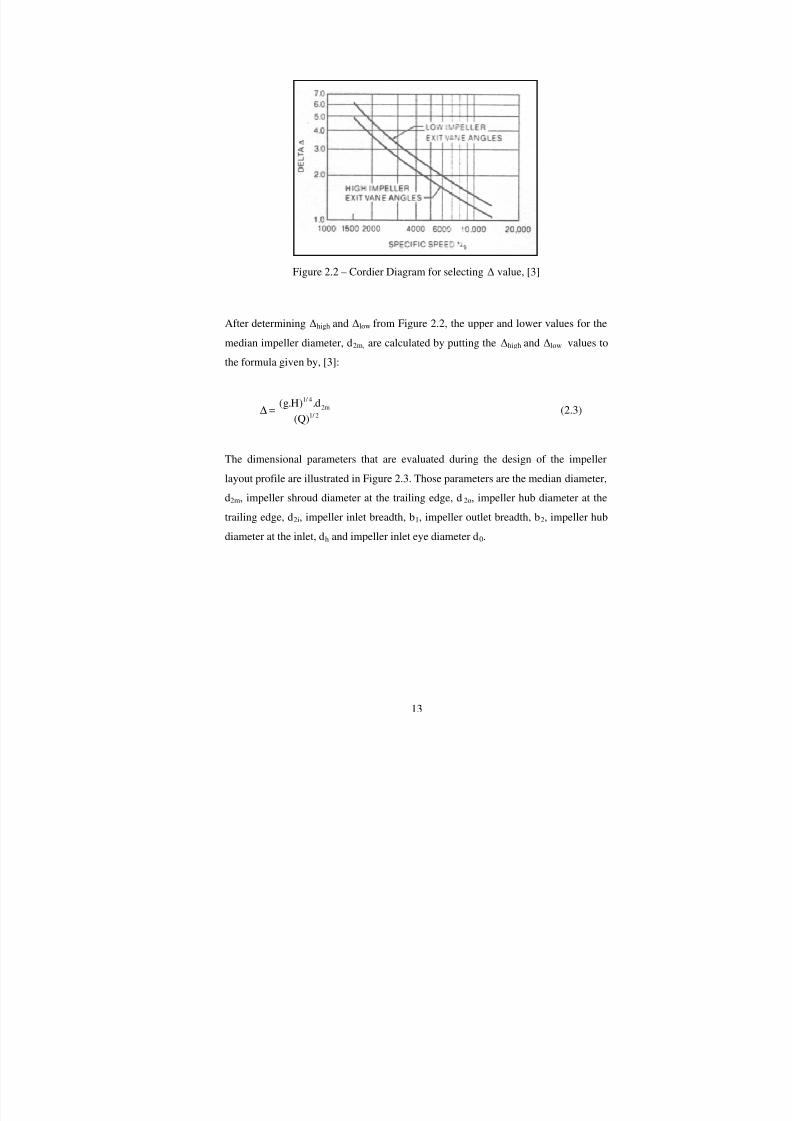
Figure 2.2 – Cordier Diagram for selecting ∆ value, [3]
After determining ∆high and ∆low from Figure 2.2, the upper and lower values for the
median impeller diameter, d2m, are calculated by putting the ∆high and ∆low values to
the formula given by, [3]:
1/ 42m
1/ 2
(g.H) .d
(Q)∆ = (2.3)
The dimensional parameters that are evaluated during the design of the impeller
layout profile are illustrated in Figure 2.3. Those parameters are the median diameter,
d2m, impeller shroud diameter at the trailing edge, d2o, impeller hub diameter at the
trailing edge, d2i, impeller inlet breadth, b1, impeller outlet breadth, b2, impeller hub
diameter at the inlet, dh and impeller inlet eye diameter d0.
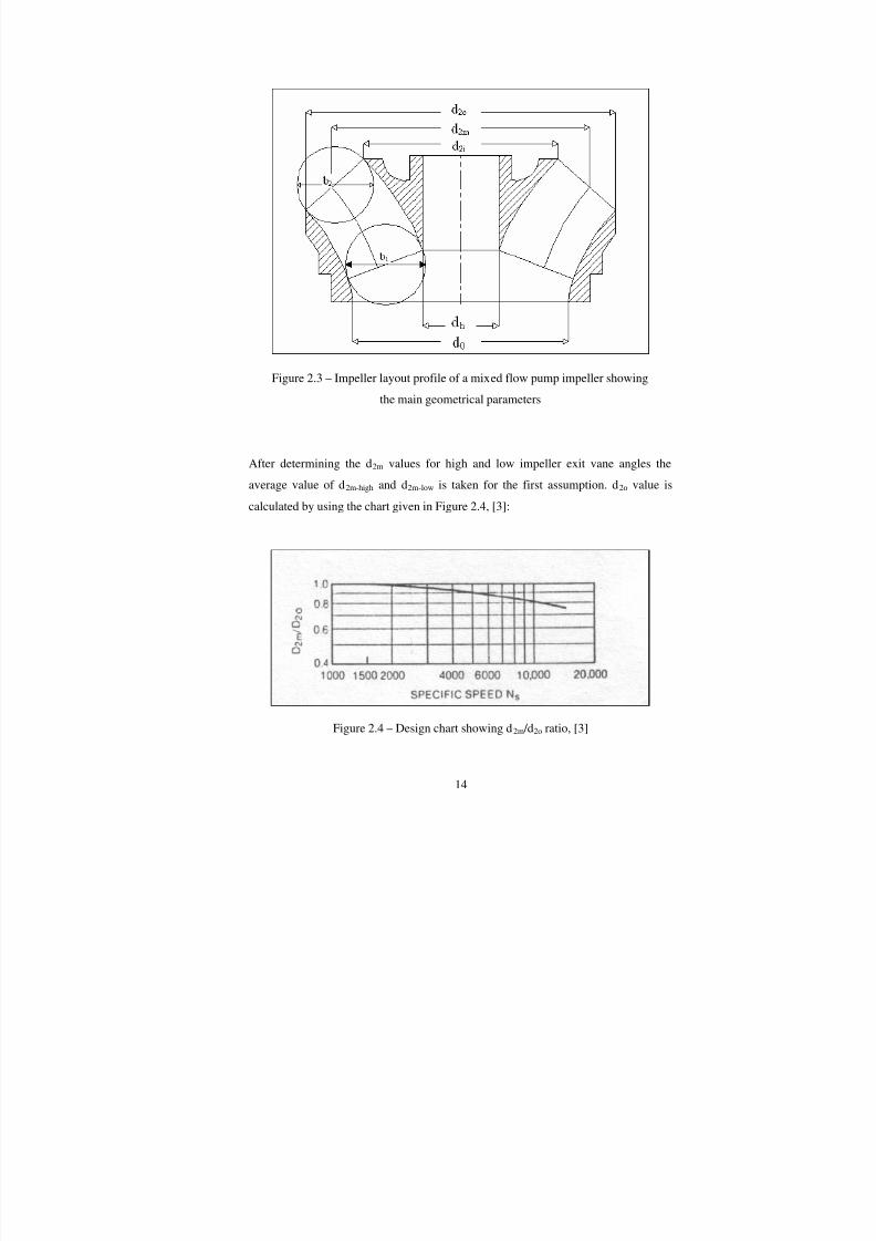
7/28/2019 design improvement of mixed flow pump through CFD.pdf
http://slidepdf.com/reader/full/design-improvement-of-mixed-flow-pump-through-cfdpdf 32/123
14
Figure 2.3 – Impeller layout profile of a mixed flow pump impeller showing
the main geometrical parameters
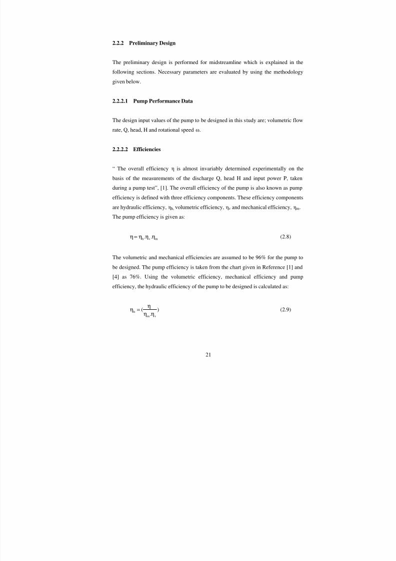
After determining the d2m values for high and low impeller exit vane angles the
average value of d2m-high and d2m-low is taken for the first assumption. d2o value is
calculated by using the chart given in Figure 2.4, [3]:
Figure 2.4 – Design chart showing d2m /d2o ratio, [3]

7/28/2019 design improvement of mixed flow pump through CFD.pdf
http://slidepdf.com/reader/full/design-improvement-of-mixed-flow-pump-through-cfdpdf 33/123
15
Found d2o and d2m values are drawn on the impeller layout in order to check the
dimensions as shown in Figure 2.5.
Figure 2.5 –Impeller layout showing found d2o and d2m-average values
d2i value, which is shown in Figure 2.3, is calculated by using the formula, [3]:
2 22o 2i
2m
(d ) + (d )d = ( )
2(2.4)
The outlet breadth, b2 is determined by using the chart shown in Figure 2.6, [3]. The
average value of the b2 is taken for the first guess. However the value is corrected
within the range shown in Figure 2.6 during the iteration procedure as explained in
the later steps of the impeller layout design. It is kept in mind that meridional
velocity at the exit depends on the value of b2. The relation of b2 and exit area is
given in the impeller exit calculation part of the preliminary design.

7/28/2019 design improvement of mixed flow pump through CFD.pdf
http://slidepdf.com/reader/full/design-improvement-of-mixed-flow-pump-through-cfdpdf 34/123
16
Figure 2.6 – Design chart showing b2 /d2m ratio
After determining the b2 value, the circle which has the radius of b2 is drawn. The
center of this circle lies at the intersection points of the d2o and existing outlet breadth
of selected profile from the library. The circle which is drawn in order to construct
the outlet breadth of the pump to be designed is shown in Figure 2.7.
Figure 2.7 – Impeller layout showing found d2o and d2i values

7/28/2019 design improvement of mixed flow pump through CFD.pdf
http://slidepdf.com/reader/full/design-improvement-of-mixed-flow-pump-through-cfdpdf 35/123
17
However in order to construct the starting point of the arc for the hub side; the shaft
size and the hub diameter should be determined. The shaft size of the impeller is
calculated for multiple stages. The selection of the stage number is made by
considering the demand for the pump to be designed from the previous sales statistics
and adding several stages to this value as safety factor. In deed, the shaft material is
also important as seen in Equation (2.5). Available shaft materials in the company
and future demands are analyzed and suitable material is selected. The selected
material is AISI 316. The diameter of the shaft is calculated, [1];
m3
s torsion
360000.Pd
.n=
τ(2.5)
where ds is the shaft diameter in cm, τs is the permissible torsion stress in kPa/cm2,
Pm is the transmitted power in Metric H.P and n is speed in rpm, [1].
The transmitted power for multiple stages, Pm, is defined as the multistage pump
power which is calculated as:
m
.g.Q.HP .m
ρ=
η(2.6)
where, m is the number of stages.
“In the U.S.S.R. the inlet diameter is calculated from the empirical formula”, [1].
The impeller inlet eye diameter is found by using this formula, [1]:
1/ 3o o
Qd K .( )
n= (2.7)
K0 term in Equation (2.7) varies between 4 and 4.5. “ K0 is selected close to the 4
where better pump efficiency is desired and K0 is selected close to the 4.5 where

7/28/2019 design improvement of mixed flow pump through CFD.pdf
http://slidepdf.com/reader/full/design-improvement-of-mixed-flow-pump-through-cfdpdf 36/123
18
better cavitation performance is desired during the design”, [20]. The K0 term is
selected close to 4 for the pump to be designed in terms of concerning better
efficiency in the design. Impeller inlet eye diameter is also shown in Figure 2.3.
The hub and shroud profiles are constructed by fitting the smooth arcs between the
impeller inlet breadth, b1, and impeller exit breadth, b2. The blade meridional profile
is extended through the impeller inlet eye in order to lower the blade number of the
impeller. The blade number of the impeller is selected to be 6 from the recent design
experience, know how coming from the company and the literature [1] and [21]. If
the blade number is higher then these values, it is hard to produce and assemble the
cores in order to obtain the impeller. The design of impeller layout then completed
with a trial and error procedure which is shown as a flow chart in Figure 2.8. The
main aim of this process is to construct the best impeller layout in order to satisfy the
flow characteristics of the pump to be designed. The unknown parameters are
eliminated by the iterative procedure coupled with the preliminary design which is
explained in the following sections. In deed the impeller layout design is highly
dependent on the previous studies and experience. Heuristic and intuitive approaches
become mainly the most important bases of the impeller layout design. Howeverthese approaches have to be supported by theoretical approaches in fluid dynamics,
numerical experimentation and experimental results. Once the desired pump
characteristics are achieved by numerical experimentation and validated by the
experimental results, the designed impeller layout is added to the impeller layout
library. The aim of creating the library is shortening the design periods of the pumps
by means of impeller layout profile design. The designer may design the impeller
layout which lies between close specific speed layouts easily if a library exists.Nevertheless the blade passage of the impeller layout may be enlarged and used if
higher flow rates are expected from an existing pump layout. This process is named
as simply building up a pump family which uses the same bowl for different
impellers with different flow rates or heads. The extension procedure is mainly done
by adjusting the exit breadth and inlet breadth of the impeller layout.

7/28/2019 design improvement of mixed flow pump through CFD.pdf
http://slidepdf.com/reader/full/design-improvement-of-mixed-flow-pump-through-cfdpdf 37/123

7/28/2019 design improvement of mixed flow pump through CFD.pdf
http://slidepdf.com/reader/full/design-improvement-of-mixed-flow-pump-through-cfdpdf 38/123
20
The designed impeller layout which is used to design the impeller is shown in Figure
2.9. The schematic representation of designed and selected impeller layout profile is
also shown in Figure 2.10.
Figure 2.9 – Designed impeller layout profile
Figure 2.10 – Schematic representation of designed and selected impeller layout
profiles
7/28/2019 design improvement of mixed flow pump through CFD.pdf
http://slidepdf.com/reader/full/design-improvement-of-mixed-flow-pump-through-cfdpdf 39/123
21
2.2.2 Preliminary Design
The preliminary design is performed for midstreamline which is explained in the
following sections. Necessary parameters are evaluated by using the methodology
given below.
2.2.2.1 Pump Performance Data
The design input values of the pump to be designed in this study are; volumetric flow
rate, Q, head, H and rotational speed ω.
2.2.2.2 Efficiencies
“ The overall efficiency η is almost invariably determined experimentally on the
basis of the measurements of the discharge Q, head H and input power P, taken
during a pump test”, [1]. The overall efficiency of the pump is also known as pump
efficiency is defined with three efficiency components. These efficiency components
are hydraulic efficiency, ηh, volumetric efficiency, ηv and mechanical efficiency, ηm.The pump efficiency is given as:
h v m. .η = η η η (2.8)
The volumetric and mechanical efficiencies are assumed to be 96% for the pump to
be designed. The pump efficiency is taken from the chart given in Reference [1] and
[4] as 76%. Using the volumetric efficiency, mechanical efficiency and pumpefficiency, the hydraulic efficiency of the pump to be designed is calculated as:
h
m v
( ).
ηη =
η η(2.9)

7/28/2019 design improvement of mixed flow pump through CFD.pdf
http://slidepdf.com/reader/full/design-improvement-of-mixed-flow-pump-through-cfdpdf 40/123
22
The general view of the impeller which is designed in the impeller layout design part
is shown in Figure 2.11. The necessary parameters are taken from the layout in order
to determine the values on the following steps of the design of the pump.
Figure 2.11 – Designed impeller layout profile
2.2.2.3 Impeller Inlet
The flow rate, Qi which is mainly defined as the volumetric flow rate passing
through the impeller blade passage is calculated using the volumetric efficiency, ηv
and the design point flow rate Q. The formula is given as, [1]:
i
v
QQ =
η(2.10)
7/28/2019 design improvement of mixed flow pump through CFD.pdf
http://slidepdf.com/reader/full/design-improvement-of-mixed-flow-pump-through-cfdpdf 41/123
23
The net area in the impeller inlet eye, A0, is calculated with considering the shaft in
the impeller inlet eye as:
2 2o s
o
.(d d )A
4
π −= (2.11)
The net impeller inlet eye diameter, do, is taken from the designed impeller layout.
The axial velocity in the impeller inlet eye which is also named as meridional
velocity is given by, [1]:
im0
0
QVA
= (2.12)
The hub diameter is taken from the impeller layout and the blade inlet area without
blade thicknesses, A1’ is calculated by revolving the blade inlet breadth, b1, around
the rotating axis. The blade thickness is the important parameter in the design. The
thickness of the blade is highly dependent on the production techniques used in the
company. If the thickness is taken too small and not adjusted with the other wallthicknesses in the impeller, casting of the impeller may not be achieved in the desired
manner. The thickness of the blade ,s , is taken as, 3 mm at leading edge, 4 mm in the
middle and 3 mm at the trailing edge of the blade.
The inlet constriction coefficient, φ1, is assumed as the first guess. The net area at the
leading edge of the blade is calculated by using, [1]:
1'1
1
AA =
ϕ(2.13)

7/28/2019 design improvement of mixed flow pump through CFD.pdf
http://slidepdf.com/reader/full/design-improvement-of-mixed-flow-pump-through-cfdpdf 42/123
24
The meridional velocity at leading edge, Vm1, of the blade is calculated as follows,
[1]:
im1
1
QV
A= (2.14)
“In order to calculate angles β1 and β2 and hence to determine the shape of the blade,
the impeller is divided into two or four (depending on the size of the impeller)
elementary streams of equal rate of flow”, [1]. The streamline which is drawn by
following the method described in Reference [1] is named as A1A2 and shown in
Figure 2.12. The design of the impeller is made for five streamlines which constitutes
to 3 streams of equal flow rate. Although the other streamlines which are between
A1A2 and hub profile and also A1A2 and shroud profile are drawn with the same
methodology.
Figure 2.12 – Designed impeller layout showing found midstreamline A1A2
7/28/2019 design improvement of mixed flow pump through CFD.pdf
http://slidepdf.com/reader/full/design-improvement-of-mixed-flow-pump-through-cfdpdf 43/123
25
The peripheral velocity at the impeller inlet is calculated as:
1
1
.dU
2
ω= (2.15)
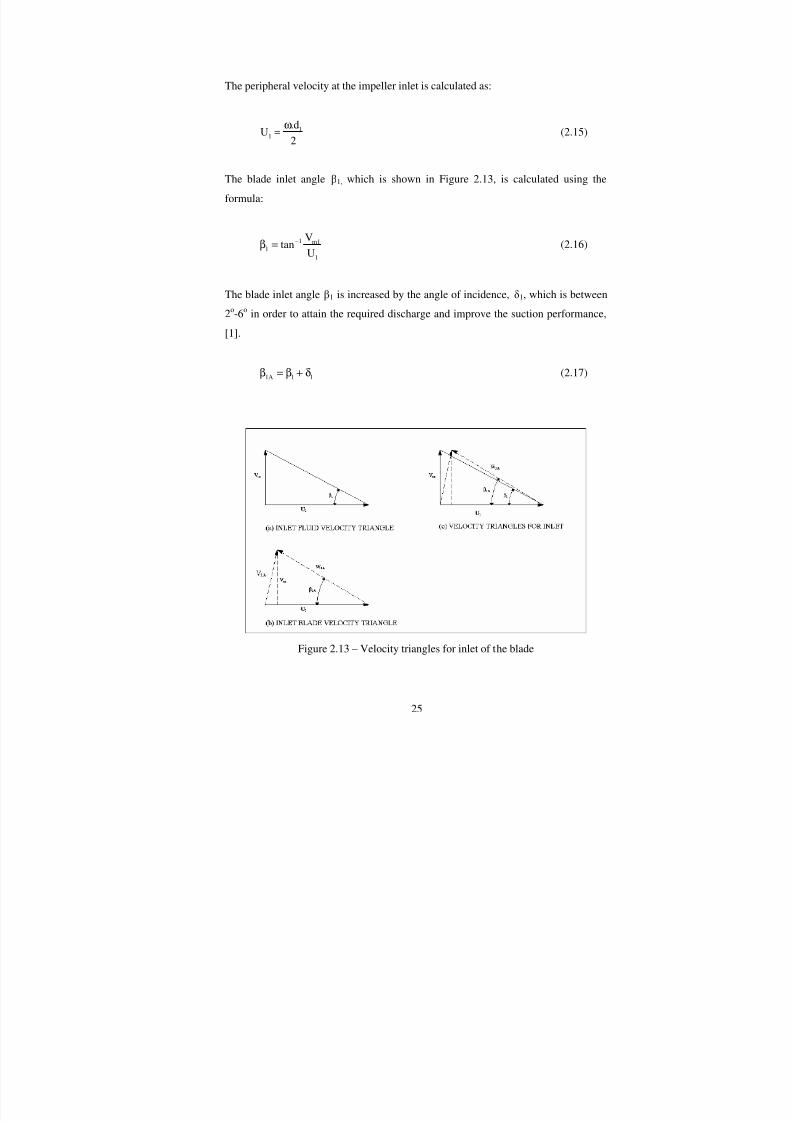
The blade inlet angle β1, which is shown in Figure 2.13, is calculated using the
formula:
1 m11
1
Vtan
U−β = (2.16)
The blade inlet angle β1 is increased by the angle of incidence, δ1, which is between
2o-6o in order to attain the required discharge and improve the suction performance,
[1].
1A 1 1β = β + δ (2.17)
Figure 2.13 – Velocity triangles for inlet of the blade
7/28/2019 design improvement of mixed flow pump through CFD.pdf
http://slidepdf.com/reader/full/design-improvement-of-mixed-flow-pump-through-cfdpdf 44/123
26
The blade number of the pump to be designed, z, is assumed in order to correct the
φ1 value with an iterative procedure. The blade number assumption is based on the
experience coming from the previous similar pump designs and the References [1]
and [21]. The arc length between the adjacent blades, t1, is calculated by the equation
given in Reference 1 by:
11
.dt
z
π= (2.18)
The correction of the φ1 is an iterative procedure. λ is the angle between the tangent
line to the hub profile and tangent line to the mid-streamline A1A2 and shown inFigure 2.11. The formula used to iterate and correct φ1 is, [1]:
1
12 2
1 1A
1
s 11 . 1
t tan ( ).sin ( )
ϕ =
− +β λ
(2.19)
Using the β1A found in Equation (2.17), φ1 is calculated and checked with the
assumed value of the φ1 in Equation (2.19). If the φ1 value found in Equation (2.19)
is different then the value used in Equation (2.13) for finding out the β1A value and
this procedure continues until the φ1 converges with the correct value of β1A.
2.2.2.4 Impeller Exit
The theoretical head, Hth, of the pump to be designed is calculated as:
th
h
HH =
η(2.20)

7/28/2019 design improvement of mixed flow pump through CFD.pdf
http://slidepdf.com/reader/full/design-improvement-of-mixed-flow-pump-through-cfdpdf 45/123
27
The blade outlet breadth, b2, is taken from the designed impeller layout. The area at
the exit of the impeller without blade thickness, A2’, is calculated by constructing the
surface with revolving b2 around the rotation axis of the impeller. The net area at the
impeller exit with blade thickness, A2, is calculated assuming the outlet constriction
coefficient, φ2, with the formula, [1]:
2'2
2
AA =
ϕ(2.21)
Meridional velocity, Vm2, is calculated as, [1]:
im2
2
QV
A= (2.22)
The peripheral velocity, U2, is calculated by using the D2 value which is the diameter
of the mid-streamline at the blade exit of the impeller by the equation:
22 .dU
2ω= (2.23)
“In order to determine the velocity U2, we use the fundamental equation for the
impeller pumps”, [1]. The fundamental equation defined in Reference 1 is basically
the form of Euler equation. The Euler equation was first introduced by L.Euler in
1754 for water turbines, [1]. Thus the angular momentum increase of the flowing
liquid is achieved by the driving motor. The torque is defined by the formula, [1]:
2 2 2 1 1 1.Q.(r .V cos r .V cos )T
g
γ α − α= (2.24)
7/28/2019 design improvement of mixed flow pump through CFD.pdf
http://slidepdf.com/reader/full/design-improvement-of-mixed-flow-pump-through-cfdpdf 46/123
7/28/2019 design improvement of mixed flow pump through CFD.pdf
http://slidepdf.com/reader/full/design-improvement-of-mixed-flow-pump-through-cfdpdf 47/123
29
m22 2
2
(V )V U
tanθ = −β
(2.27)
When 2Vθ is put into Equation (2.26) the following formula is achieved:
m2th 2 2 1 1
2
Vg.H U (U ) V U
tan∞ θ= − −β
(2.28)
Assuming no-inlet whirl condition for the inlet of the blade of the impeller, then
1 1V .Uθ term becomes zero. The Equation (2.28) reduces to:
m2th 2 2
2
Vg.H U (U )
tan∞ = −
β(2.29)
The positive root of this equation is taken in order to determine the U2 value as:
2m2 m2
2 th2 2
V V
U ( ) gH2 tan 2 tan ∞= + +β β (2.30)
Since the theoretical head for infinite number of blades is, [1]:
( )th th pH H . 1 C∞ = + (2.31)
where, Cp is the Pfleiderer’s correction factor. Cp is used as a value which lies
between 0.25 and 0.35 in preliminary calculations, [1]. Then Equation (2.30)
becomes:
( )2m2 m22 th p
2 2
V VU ( ) gH . 1 C
2 tan 2 tan= + + +
β β(2.32)

7/28/2019 design improvement of mixed flow pump through CFD.pdf
http://slidepdf.com/reader/full/design-improvement-of-mixed-flow-pump-through-cfdpdf 48/123
7/28/2019 design improvement of mixed flow pump through CFD.pdf
http://slidepdf.com/reader/full/design-improvement-of-mixed-flow-pump-through-cfdpdf 49/123
31
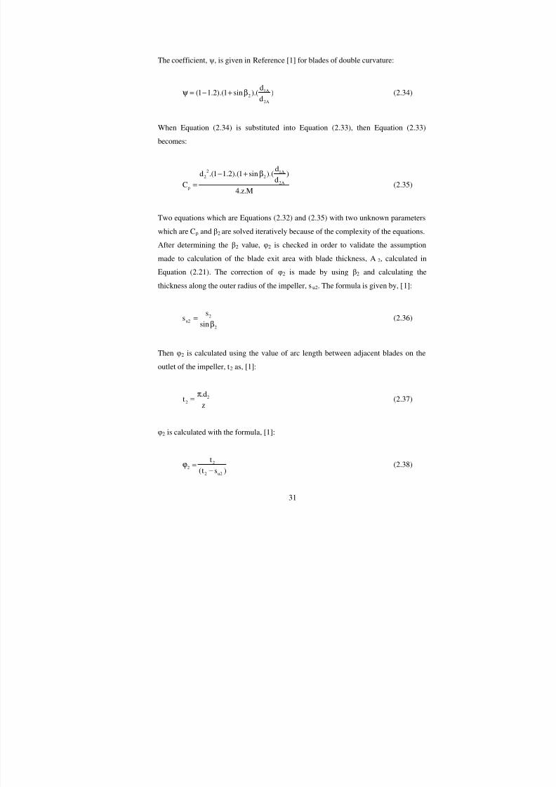
The coefficient, ψ, is given in Reference [1] for blades of double curvature:
1A
2 2A
d(1 1.2).(1 sin ).( )
dψ = − + β (2.34)
When Equation (2.34) is substituted into Equation (2.33), then Equation (2.33)
becomes:
2 1A2 2
2Ap
dd .(1 1.2).(1 sin ).( )
dC
4.z.M
− + β
= (2.35)
Two equations which are Equations (2.32) and (2.35) with two unknown parameters
which are Cp and β2 are solved iteratively because of the complexity of the equations.
After determining the β2 value, φ2 is checked in order to validate the assumption
made to calculation of the blade exit area with blade thickness, A2, calculated in
Equation (2.21). The correction of φ2 is made by using β2 and calculating the
thickness along the outer radius of the impeller, su2. The formula is given by, [1]:
2u2
2
ss
sin=
β(2.36)
Then φ2 is calculated using the value of arc length between adjacent blades on the
outlet of the impeller, t2 as, [1]:
22
.dt
z
π= (2.37)
φ2 is calculated with the formula, [1]:
22
2 u2
t
(t s )ϕ =
−(2.38)

7/28/2019 design improvement of mixed flow pump through CFD.pdf
http://slidepdf.com/reader/full/design-improvement-of-mixed-flow-pump-through-cfdpdf 50/123

7/28/2019 design improvement of mixed flow pump through CFD.pdf
http://slidepdf.com/reader/full/design-improvement-of-mixed-flow-pump-through-cfdpdf 51/123
33
2.2.3 Shaping the Blades of Impeller
There are several methods in the literature for shaping the blades of the impeller. In
this study, point by point method which is introduced by C. Pfleiderer is used. The
blade of the impeller is shaped by adjusting the distributions of the velocity
components from leading edge to the trailing edge of the blade. Nevertheless, the
blade angle distribution should be checked from leading edge to trailing edge of the
blade. The distributions are adjusted in order to find out better blade angle
distribution or stacking condition on the blade exit. The stacking condition is the
position of the blade at trailing edge from hub to shroud. The impellers that are
produced in the company have different configuration of stacking conditions.
However, in this study the stacking is adjusted by means of following the linear
distribution of relative velocity from leading edge to trailing edge for each streamline
that are used in the design. The distributions by means of relative velocity,
meridional velocity and blade angle for mid-streamline A1A2 is shown in the
following Figure 2.16.
Figure 2.16 – The distributions of relative velocity, meridional velocity and blade
angle for mid-streamline A1A2

7/28/2019 design improvement of mixed flow pump through CFD.pdf
http://slidepdf.com/reader/full/design-improvement-of-mixed-flow-pump-through-cfdpdf 52/123
34
The designed impeller blade represented with midstreamline A1A2 from top view is
shown in Figure 2.17. The swirl angle which is between the starting point and end
point of the midstreamline is seen also in Figure 2.16.
Figure 2.17 – Designed impeller blade showing found midstreamline A1A2 from top
view
2.3 Design of the Bowl
The main function of the bowl used in vertical turbine pump that is designed in this
study is, changing the direction of flow of the liquid leaving the impeller and
directing the flow along the axis of rotation. However while changing the direction
of flow; the design should minimize the losses inside the bowl. In order to satisfy this
need, the bowl should be designed not too long that may increase the friction losses
and not too short that may cause the flow not to be directed properly to the second
stage.

7/28/2019 design improvement of mixed flow pump through CFD.pdf
http://slidepdf.com/reader/full/design-improvement-of-mixed-flow-pump-through-cfdpdf 53/123
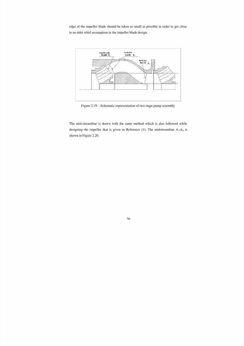
7/28/2019 design improvement of mixed flow pump through CFD.pdf
http://slidepdf.com/reader/full/design-improvement-of-mixed-flow-pump-through-cfdpdf 54/123
7/28/2019 design improvement of mixed flow pump through CFD.pdf
http://slidepdf.com/reader/full/design-improvement-of-mixed-flow-pump-through-cfdpdf 55/123
37
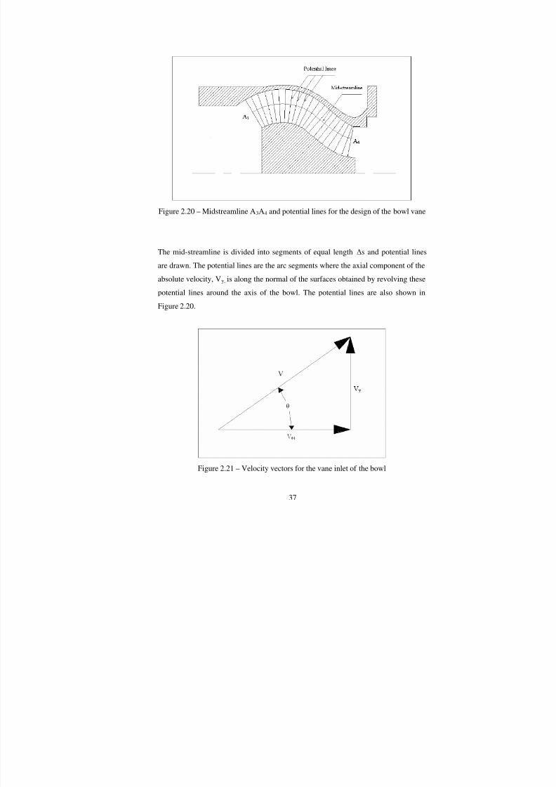
Figure 2.20 – Midstreamline A3A4 and potential lines for the design of the bowl vane
The mid-streamline is divided into segments of equal length ∆s and potential lines
are drawn. The potential lines are the arc segments where the axial component of the
absolute velocity, Vy, is along the normal of the surfaces obtained by revolving these
potential lines around the axis of the bowl. The potential lines are also shown inFigure 2.20.
Figure 2.21 – Velocity vectors for the vane inlet of the bowl
7/28/2019 design improvement of mixed flow pump through CFD.pdf
http://slidepdf.com/reader/full/design-improvement-of-mixed-flow-pump-through-cfdpdf 56/123
38
The tangential component of the velocity at the blade exit for the flowing fluid, V θ3,
as shown in Figure 2.21 is calculated as:
23
p
VV
(1 C )θ
θ =+
(2.41)
The fluid angle leaving the impeller, θ3, is calculated by:
m23
3
Vtan
Vθ
θ = (2.42)
The arc length between adjacent vanes of the bowl for inlet, t4 is calculated as, [1]:
s4
b
.Dt
z
π= (2.43)
where Ds is the diameter of the streamline and zb is the vane number of the bowl.
The vane inlet angle, θ4, is calculated using the formula, [1]:
44 3
v4
3
ttan tan .
s(t )
sin
θ = θ
−θ
(2.44)
where, sv is the vane thickness of the bowl. Constant vane thickness of 4 mm is taken
for the bowl vane in the bowl design. The thickness along the direction of the flow
for the inlet of the bowl, su3, is calculated as:
4u4
4
ss
sin=
θ(2.45)

7/28/2019 design improvement of mixed flow pump through CFD.pdf
http://slidepdf.com/reader/full/design-improvement-of-mixed-flow-pump-through-cfdpdf 57/123
39
The inlet constriction coefficient of the bowl, φ4, is calculated with the formula, [1]:
4
4 4 u4
t
(t s )ϕ =
−(2.46)
The axial component of the absolute velocity, Vy, is calculated using the formula:
y 4
4
QV .
A= ϕ (2.47)
A4 is the net area obtained by revolving the bowl inlet vane breadth around bowlcenter axis. The tangential component of the absolute velocity, Vθ5 is calculated by
the formula given as:
y4
4
VV
tanθ =θ
(2.48)
The point by point method is followed for shaping the vane of the bowl. Since theflowing liquid enters the impeller in the second stage with no inlet whirl condition,
the flow is in the direction of axis of rotation which means the tangential component
of the absolute velocity, Vθ5, should be zero at the exit of the bowl vane. The vane of
the bowl is shaped by considering the distribution of Vθ through out the equal
distanced segments from inlet to outlet. The distribution of Vθ is adjusted by the
designer by looking at the previous designs by considering the specific speed and the
flow rate of the design point of view. On the other hand, the distribution of Vθ between the inlet and exit of the bowl vane is adjusted by considering the swept
angle. Swept angle is the angle between the inlet and outlet of each streamline
between the inlet and outlet from the top view. The main reason of considering the
swept angle is due to manufacturing. If the swept angle is relatively high, the
placement of the patterns may not be possible while preparing the core of the bowl.

7/28/2019 design improvement of mixed flow pump through CFD.pdf
http://slidepdf.com/reader/full/design-improvement-of-mixed-flow-pump-through-cfdpdf 58/123

7/28/2019 design improvement of mixed flow pump through CFD.pdf
http://slidepdf.com/reader/full/design-improvement-of-mixed-flow-pump-through-cfdpdf 59/123

7/28/2019 design improvement of mixed flow pump through CFD.pdf
http://slidepdf.com/reader/full/design-improvement-of-mixed-flow-pump-through-cfdpdf 60/123
7/28/2019 design improvement of mixed flow pump through CFD.pdf
http://slidepdf.com/reader/full/design-improvement-of-mixed-flow-pump-through-cfdpdf 61/123
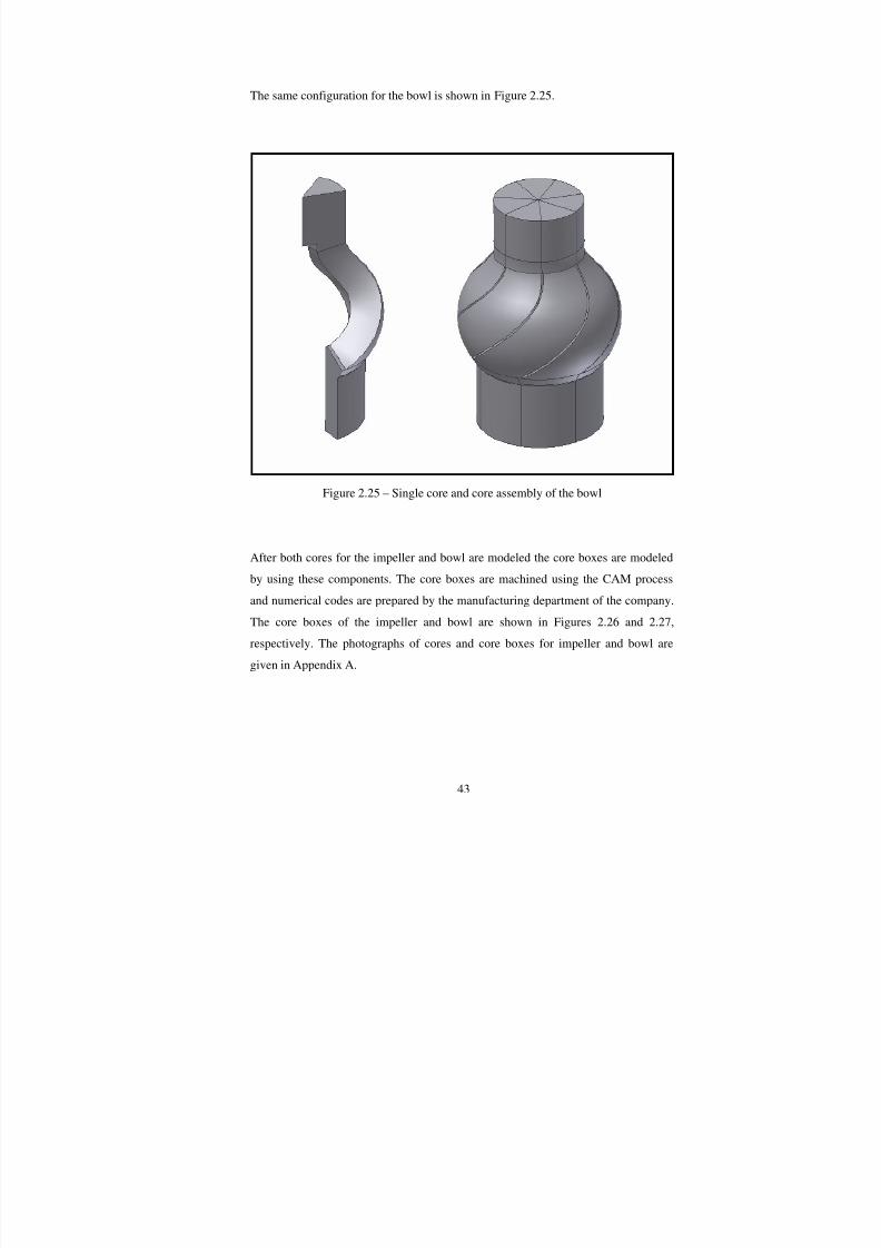
43
The same configuration for the bowl is shown in Figure 2.25.
Figure 2.25 – Single core and core assembly of the bowl
After both cores for the impeller and bowl are modeled the core boxes are modeled
by using these components. The core boxes are machined using the CAM process
and numerical codes are prepared by the manufacturing department of the company.
The core boxes of the impeller and bowl are shown in Figures 2.26 and 2.27,
respectively. The photographs of cores and core boxes for impeller and bowl are
given in Appendix A.

7/28/2019 design improvement of mixed flow pump through CFD.pdf
http://slidepdf.com/reader/full/design-improvement-of-mixed-flow-pump-through-cfdpdf 62/123
44
Figure 2.26 – Core box of the impeller
Figure 2.27 – Core box of the bowl
The cores are produced by using the core machine where the core boxes are used.
The produced cores are assembled together and the casting is made.

7/28/2019 design improvement of mixed flow pump through CFD.pdf
http://slidepdf.com/reader/full/design-improvement-of-mixed-flow-pump-through-cfdpdf 63/123
45
CHAPTER 3
CFD ANALYSES OF THE PUMP
3.1 General Information on CFD Analyses and Software
In order to shorten the design periods and lowering the manufacturing, prototyping
and test costs of the pump, a commercial Computational Fluid Dynamics (CFD)
software is used in the design procedure. The main aim of this study by means of
applying numerical experimentation to the designed pump is CFD code integrationinto the design procedure and verification of the design before the pump is produced.
The CFD code is used to obtain pump characteristics curves such as head vs. flow
rate and efficiency vs. flow rate. In deed, investigations of the internal flow structure
are also performed in order to correct the design and obtain better performance
characteristics from the designed pump. The flow inside the impeller and bowl is
studied by using the capabilities of CFD code used in the company such as pathline
traces, velocity vector representations, and physical quantities such as pressure andvelocity distributions inside the pump which are explained in the following parts of
Chapter 3. However, before the CFD software is integrated into the design
procedure, the verification of the code is done by applying CFD analyses to the
previously designed pumps. The comparison of the CFD results is made with the
calibrated and certified test stand of the company.
The conventional design and CFD integrated design procedures are shown in Figure
3.1. The CFD code is used as a tool in the design and verification of the physical
quantities are cross checked with the design parameters.

7/28/2019 design improvement of mixed flow pump through CFD.pdf
http://slidepdf.com/reader/full/design-improvement-of-mixed-flow-pump-through-cfdpdf 64/123

7/28/2019 design improvement of mixed flow pump through CFD.pdf
http://slidepdf.com/reader/full/design-improvement-of-mixed-flow-pump-through-cfdpdf 65/123
47
to get the desired efficiency. However those operations may increase the design
periods and overall costs of the pump.
When the CFD software is integrated into the design procedure, the designer may use
the code as a tool in the design. After designing the pump, CFD analyses are
performed and the best performance characteristics may be achieved without
producing the prototype if the code is validated by the experimental results. Since
CFD code is a tool in the design step, the verification should be done in each case
study and the behavior of the code should be investigated for different types of the
pumps by means of specific speed, flow rate and geometry.
The pump that is designed in this study is analyzed by using two different CAD
models of the impeller. The first one is the impeller with designed blade and the
second one is the impeller with underfiled blades. “For best results with pump design
it is very important that the vane trailing edge be made as thin as possible”, [19]. The
underfiling operation frequently increases the efficiency and head at the best
efficiency point of the pumps that are previously designed and tested in the company.
Commercial CFD software solves 6 equations which are mainly conservation of
mass, conservation of momentum in three principle directions, energy equations
apply to the laminar as well as turbulent flow and turbulence equations. The solution
of these equations involves an iterative procedure and requires great deal of elements
in order to properly model the flow. Nevertheless, the computing power is an
important fact in CFD analyses both for modeling the flow geometry and solving the
equations. A desktop PC which has a Pentium 4 3.2 GHz processor with 2 GB RAMin 32 bit environment is used for the analyses. The memory of the computer involves
in modeling of the flow geometry which is related to grid size and solution speed is
proportional to the clock speed of the processor. Computers with faster processors
and high capacity of memories may shorten the analyses solution periods. However
the analysis strategy is playing a major role in shorten the solution periods. The
instabilities occurring during the analyses are directly affected by the improper grid

7/28/2019 design improvement of mixed flow pump through CFD.pdf
http://slidepdf.com/reader/full/design-improvement-of-mixed-flow-pump-through-cfdpdf 66/123
48
size and flow geometry. The turbomachinery CFD solutions are one of the difficult
solutions in CFD because of the nature of the flow and complexity of the geometries.
CFdesign V7 and V8 are used in CFD analyses. CFdesign solves time averaged
governing equations which are stated above. “In CFdesign, the finite element method
is used to reduce the governing partial differential equations to set of algebraic
equations”, [13]. “CFdesign uses the finite element method primarily because of its
flexibility in modeling any geometrical shape”, [13]. Since the geometry of the
pump is very complex, the code is chosen for the analysis tool in the company.
The solution algorithm of CFdesign is based on Semi Implicit Method for Pressure
Linked Equations Revised (SIMPLE-R).
The automatic mesh generator and diagnostics in mesh generation is used in
CFdesign. Diagnostics module shows the solid model parts where problems may
occur during the mesh generation. The quadrilateral, triangular, tetrahedral,
hexahedral, wedge and pyramid elements are available in CFdesign mesh generator
module for the analyses of fluid flow, [13]. The boundary layer is controlled by theboundary layer thickness factor located in the mesh enhancement module of
CFdesign. The thickness of the layer near the wall and the number of layers within
this layer may be adjusted. “Mesh Enhancement is a great feature that considerably
simplifies the mesh definition process. Mesh Enhancement automatically constructs
layers of prismatic elements (extruded triangles) along all walls and all fluid-solid
interfaces in the model, based on the tetrahedral mesh that is defined. These
additional elements serve two primary purposes; elements are concentrated in theboundary layer region, where high velocity, pressure, and turbulence gradients most
often occur and enough nodes are automatically placed in all gaps (area between
walls) in the model.”, [13].
The RNG model, low Reynolds k-epsilon model, k-epsilon model and Eddy
Viscosity models are available in CFdesign. The k-epsilon model is used in this

7/28/2019 design improvement of mixed flow pump through CFD.pdf
http://slidepdf.com/reader/full/design-improvement-of-mixed-flow-pump-through-cfdpdf 67/123

7/28/2019 design improvement of mixed flow pump through CFD.pdf
http://slidepdf.com/reader/full/design-improvement-of-mixed-flow-pump-through-cfdpdf 68/123
50
Figure 3.2 – Figure showing the extensions and rotating region for CFD analysis in
the section view representation of the pump
The solid models are kept as simple as possible in order to simplify the analyses.
Nevertheless the parts which are suction bell, impeller and bowl are modeled in their
original forms in order not to disturb the hydraulic performance of the pump to be
simulated in CFD. The solid models are shown in Figure 3.3.

7/28/2019 design improvement of mixed flow pump through CFD.pdf
http://slidepdf.com/reader/full/design-improvement-of-mixed-flow-pump-through-cfdpdf 69/123
5 1
Figure 3.3 – Solid models prepared for the pump and pump assembly
7/28/2019 design improvement of mixed flow pump through CFD.pdf
http://slidepdf.com/reader/full/design-improvement-of-mixed-flow-pump-through-cfdpdf 70/123
52
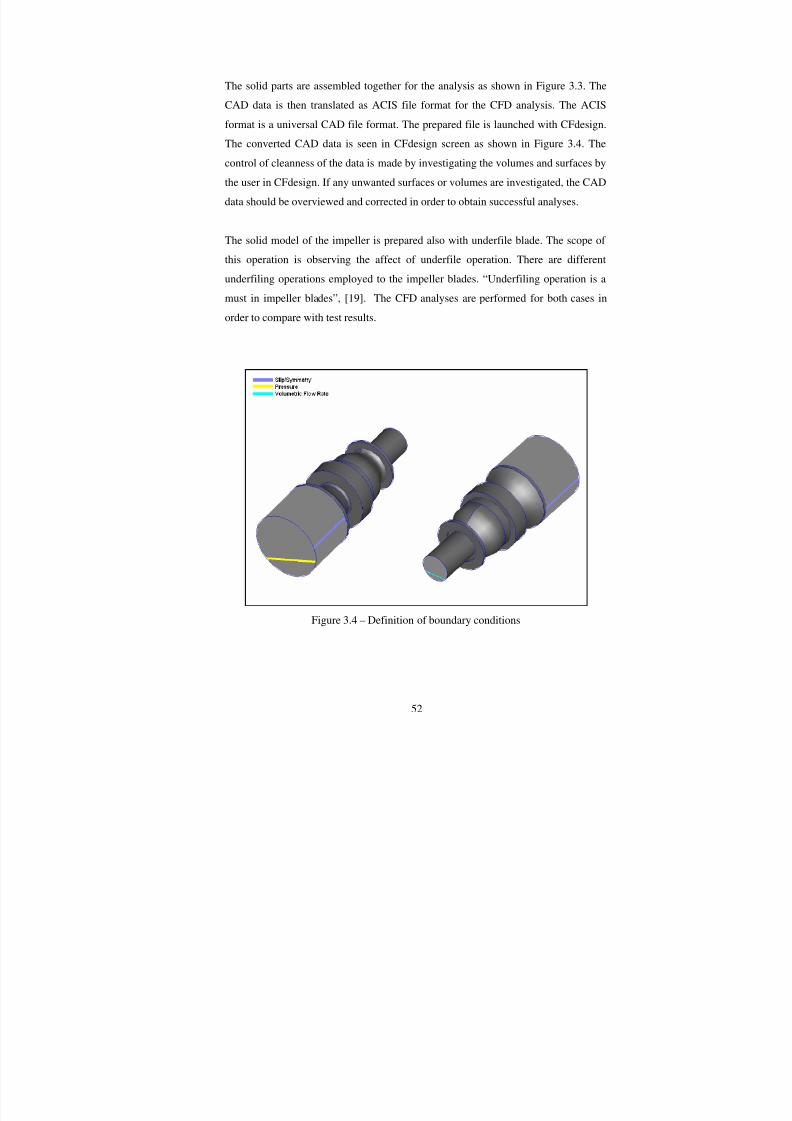
The solid parts are assembled together for the analysis as shown in Figure 3.3. The
CAD data is then translated as ACIS file format for the CFD analysis. The ACIS
format is a universal CAD file format. The prepared file is launched with CFdesign.
The converted CAD data is seen in CFdesign screen as shown in Figure 3.4. The
control of cleanness of the data is made by investigating the volumes and surfaces by
the user in CFdesign. If any unwanted surfaces or volumes are investigated, the CAD
data should be overviewed and corrected in order to obtain successful analyses.
The solid model of the impeller is prepared also with underfile blade. The scope of
this operation is observing the affect of underfile operation. There are different
underfiling operations employed to the impeller blades. “Underfiling operation is a
must in impeller blades”, [19]. The CFD analyses are performed for both cases in
order to compare with test results.
Figure 3.4 – Definition of boundary conditions

7/28/2019 design improvement of mixed flow pump through CFD.pdf
http://slidepdf.com/reader/full/design-improvement-of-mixed-flow-pump-through-cfdpdf 71/123
53
3.2.2 Definition of Boundary Conditions
The pressure rise across the inlet and outlet of the pump is aimed to be found through
out the analyses. In order to find the pressure rise, the volumetric flow rate is defined
at the outlet of the pump and 0 gage pressure is defined at the inlet of the pump. In
real life experiments the pump is submerged into the large reservoir. Defining the
slip/symmetry boundary condition to the lateral surface of the lower extension
simulates this condition in CFD analyses. The pipe is connected to the outlet flange
of the bowl at the upper part of the pump assembly in experiments. Thus no
boundary condition definitions are applied to the lateral surface of the upper
extension. The boundary condition definitions are shown in Figure 3.4.
3.2.3 Mesh Generation
The fluid structure which is formed by placing the extensions to the inlet and outlet
of the pump is divided into finite elements. “Prior to running a CFdesign analysis,
the geometry has to be broken up into small, manageable pieces called elements. Thecorner of each element is called a node, and it is at each node that a calculation is
performed. All together these elements and nodes comprise the mesh (also known as
the finite element mesh )”, [13]. In order to achieve reliable solutions in CFD
analyses the number of elements should be increased as much as possible. However
when the total number of elements increased, the solution periods become longer. On
the other hand, 32 bit environment does not allow using more then 2 GB of memory
in the computer hardware. The mesh independency can not be investigated in theturbomachinery CFD analyses, [14]. The grid size used in this study is the result of
the recent studies and completed projects with CFdesign.
The meshing strategy is simply, using smaller elements for the impeller and
surrounding rotating region and increasing the element size for the other parts. The
starting point of the impeller meshing is defining the element size which is closer to
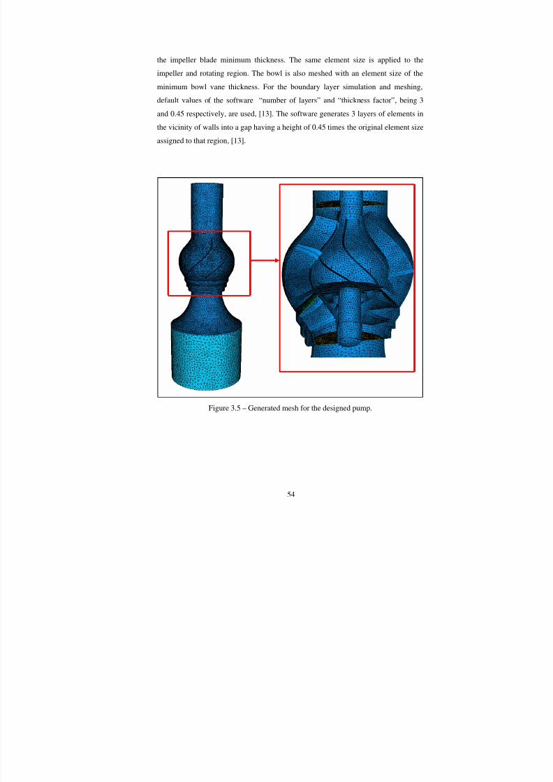
7/28/2019 design improvement of mixed flow pump through CFD.pdf
http://slidepdf.com/reader/full/design-improvement-of-mixed-flow-pump-through-cfdpdf 72/123

7/28/2019 design improvement of mixed flow pump through CFD.pdf
http://slidepdf.com/reader/full/design-improvement-of-mixed-flow-pump-through-cfdpdf 73/123

7/28/2019 design improvement of mixed flow pump through CFD.pdf
http://slidepdf.com/reader/full/design-improvement-of-mixed-flow-pump-through-cfdpdf 74/123

7/28/2019 design improvement of mixed flow pump through CFD.pdf
http://slidepdf.com/reader/full/design-improvement-of-mixed-flow-pump-through-cfdpdf 75/123
57
volumetric flow rate values are 60 l/s, 70 l/s, 90 l/s, 100 l/s, 120 l/s and 135 l/s. The
pump in Case 1 is also solved for 1450 rpm rotational speed of the impeller. The
volumetric flow rate of 30 l/s, 35 l/s, 45 l/s, 50 l/s, 55 l/s and 60 l/s are defined in
order to simulate different operating points at 1450 rpm. Each analysis is run for 680
iterations and each analysis takes 39 hours for single operating point.
The convergence of the analysis is followed from the convergence monitor of the
CFdesign as shown in Figure 3.7. The convergence monitor shows the summary and
the average value of each degree of freedom in the analysis, [13]. The pressure and
velocity component in the direction of the flow at the outlet flange plane of the bowl
are expected to become straight lines in order to have convergence in the analysis.
The software records the results for defined intervals. The convergence is also
investigated manually by taking the pressure, velocity and hydraulic torque values
from cut-planes close to the outlet and inlet of the pump for these intervals. These
values are taken for the saved intervals from the beginning to the end of the analysis
and convergence is checked by tabulating these values. When the taken values
converge the convergence assessment is done.
Figure 3.7 – Sample Convergence Monitor for the CFD Analysis
In order to find out the total head of the pump the Bernoulli equation is written
between the cut-plane 1 and cut-plane 2 as seen in the figure.

7/28/2019 design improvement of mixed flow pump through CFD.pdf
http://slidepdf.com/reader/full/design-improvement-of-mixed-flow-pump-through-cfdpdf 76/123
58
2 21 1 2 2
e
p V p VH h
.g 2.g .g 2.g+ + = + +
ρ ρ(3.1)
where p1 is the pressure value and V1 is the mean velocity in the cut-plane 1, p2 is the
pressure value and V2 is the mean velocity in the cut-plane, h is the head of the pump
and he is the elevation difference between cut-plane 1 and cut-plane 2 as shown in
Figure 3.8.
Figure 3.8 – Cut-planes used to calculated the head of the pump
The torque value is read from the CFdesign torque output file. The hydraulic
efficiency of the pump is found in the analysis. The gap between the impeller and
casing is closed in order not to increase the number of elements used in the analysis.
Since the gap between the impeller and casing is between 0.4 to 1 mm in these kinds
of pumps, it is not necessary to mesh this volume for the sake of number of elements
to be used. If the gap is meshed the number of elements is exceeded to the level
7/28/2019 design improvement of mixed flow pump through CFD.pdf
http://slidepdf.com/reader/full/design-improvement-of-mixed-flow-pump-through-cfdpdf 77/123
59
where 32 bit environment can handle. However the volumetric efficiency and the
mechanical efficiency are used as the same values assumed in the early steps of
design of the impeller in order to calculate the pump efficiency. The hydraulic
efficiency is calculated by the formula given by:
waterh
.g.Q.H
T.
ρη =
ω(3.2)
The flow in the impeller is investigated by using the velocity vector representation of
CFdesign for 120 l/s at 2900 rpm. The single blade to blade passage of the impeller is
investigated visually for flow separation. Since CFdesign does not have themeridional view representation, if the pump performance is lower then what is
expected in the design, the flow inside the impeller and bowl is investigated by the
help of post processor functions of CFdesign. If any backflows or separations occur
in the impeller blade passage or bowl vane passage, the unexpected flow motion is
captured by using these functions of CFdesign after the analysis is converged. The
pressure side of the impeller blade is projected to the suction side of the blade. The
relative velocity vectors are shown in different positions of the projected surface inFigure 3.9. In this figure the relative velocity vectors which are colored with absolute
velocity values are represented.

7/28/2019 design improvement of mixed flow pump through CFD.pdf
http://slidepdf.com/reader/full/design-improvement-of-mixed-flow-pump-through-cfdpdf 78/123
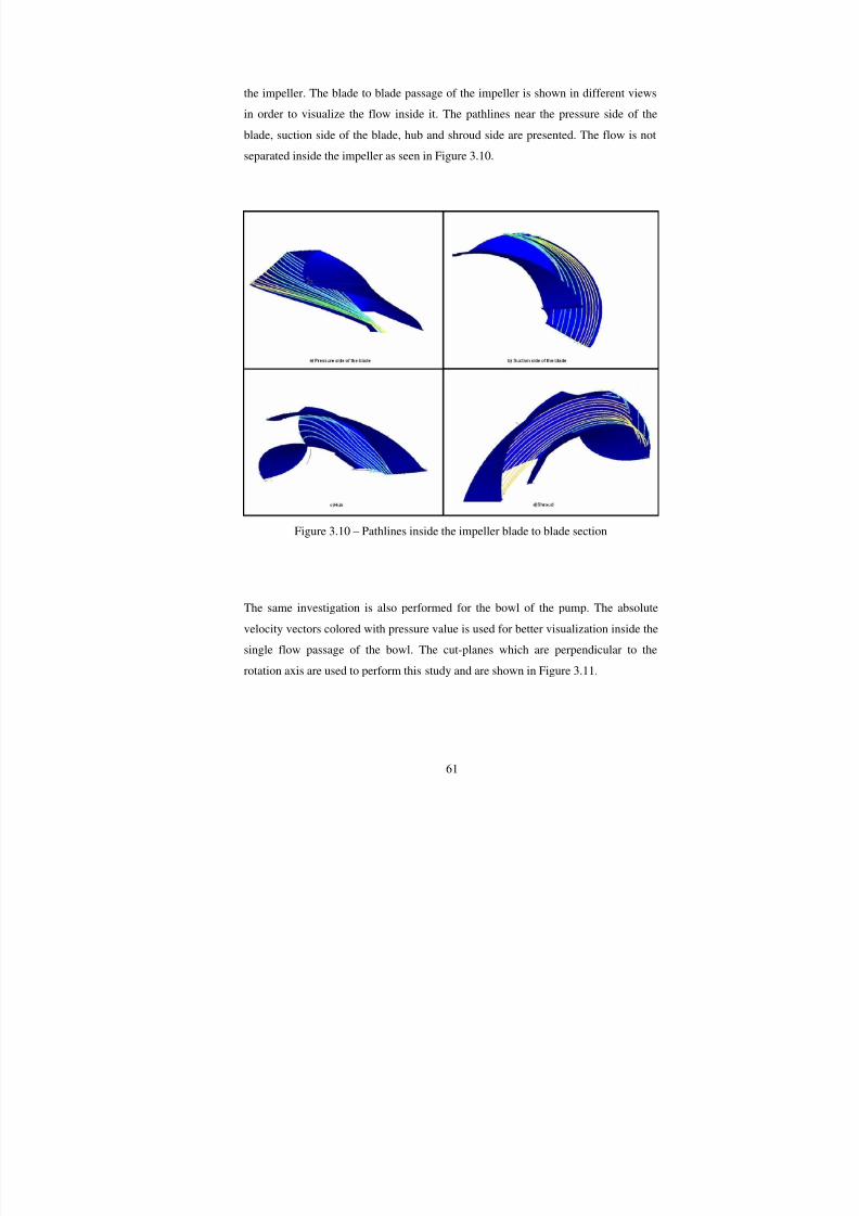
7/28/2019 design improvement of mixed flow pump through CFD.pdf
http://slidepdf.com/reader/full/design-improvement-of-mixed-flow-pump-through-cfdpdf 79/123
61
the impeller. The blade to blade passage of the impeller is shown in different views
in order to visualize the flow inside it. The pathlines near the pressure side of the
blade, suction side of the blade, hub and shroud side are presented. The flow is not
separated inside the impeller as seen in Figure 3.10.
Figure 3.10 – Pathlines inside the impeller blade to blade section
The same investigation is also performed for the bowl of the pump. The absolute
velocity vectors colored with pressure value is used for better visualization inside the
single flow passage of the bowl. The cut-planes which are perpendicular to the
rotation axis are used to perform this study and are shown in Figure 3.11.
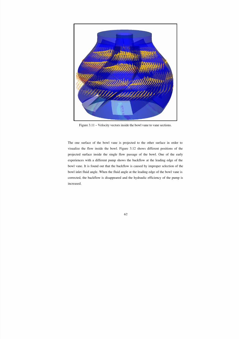
7/28/2019 design improvement of mixed flow pump through CFD.pdf
http://slidepdf.com/reader/full/design-improvement-of-mixed-flow-pump-through-cfdpdf 80/123
62
Figure 3.11 – Velocity vectors inside the bowl vane to vane sections.
The one surface of the bowl vane is projected to the other surface in order to
visualize the flow inside the bowl. Figure 3.12 shows different positions of the
projected surface inside the single flow passage of the bowl. One of the early
experiences with a different pump shows the backflow at the leading edge of the
bowl vane. It is found out that the backflow is caused by improper selection of thebowl inlet fluid angle. When the fluid angle at the leading edge of the bowl vane is
corrected, the backflow is disappeared and the hydraulic efficiency of the pump is
increased.
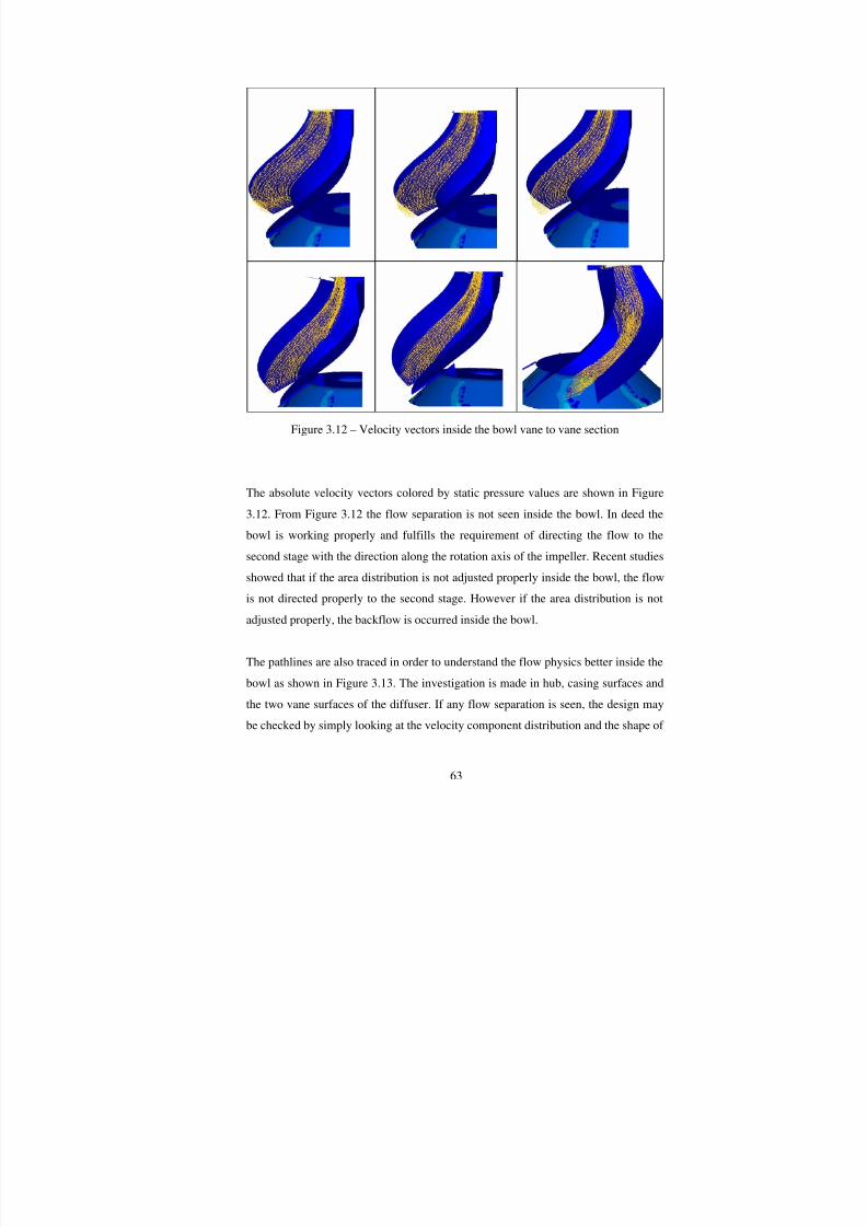
7/28/2019 design improvement of mixed flow pump through CFD.pdf
http://slidepdf.com/reader/full/design-improvement-of-mixed-flow-pump-through-cfdpdf 81/123
63
Figure 3.12 – Velocity vectors inside the bowl vane to vane section
The absolute velocity vectors colored by static pressure values are shown in Figure
3.12. From Figure 3.12 the flow separation is not seen inside the bowl. In deed the
bowl is working properly and fulfills the requirement of directing the flow to the
second stage with the direction along the rotation axis of the impeller. Recent studies
showed that if the area distribution is not adjusted properly inside the bowl, the flow
is not directed properly to the second stage. However if the area distribution is not
adjusted properly, the backflow is occurred inside the bowl.
The pathlines are also traced in order to understand the flow physics better inside the
bowl as shown in Figure 3.13. The investigation is made in hub, casing surfaces and
the two vane surfaces of the diffuser. If any flow separation is seen, the design may
be checked by simply looking at the velocity component distribution and the shape of

7/28/2019 design improvement of mixed flow pump through CFD.pdf
http://slidepdf.com/reader/full/design-improvement-of-mixed-flow-pump-through-cfdpdf 82/123
64
the bowl vane layout. The continuity of the profile by means of bowl and impeller
should be checked by the designer.
Figure 3.13 – Pathlines inside the bowl vane to vane section
From the previous studies, there are several regions where the flow can be disturbed
and showed recirculation in the bowl. The first region is the vane inlet. If the flow
angle is not adjusted properly at the leading edge of the vane, separation on may
occur. The other region is close to the bowl outlet. If the length of the bowl and theswept angle are not adjusted properly, the flow may show recirculation. On the other
hand due to formation of secondary flows in the bowl close to the bowl exit, the flow
can not be directed properly to the second stage and this affects the hydraulic
characteristics of the pump.

7/28/2019 design improvement of mixed flow pump through CFD.pdf
http://slidepdf.com/reader/full/design-improvement-of-mixed-flow-pump-through-cfdpdf 83/123
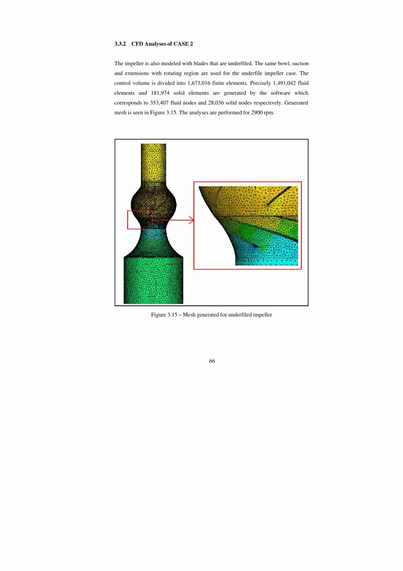
7/28/2019 design improvement of mixed flow pump through CFD.pdf
http://slidepdf.com/reader/full/design-improvement-of-mixed-flow-pump-through-cfdpdf 84/123
66
3.3.2 CFD Analyses of CASE 2
The impeller is also modeled with blades that are underfiled. The same bowl, suction
and extensions with rotating region are used for the underfile impeller case. The
control volume is divided into 1,673,016 finite elements. Precisely 1,491,042 fluid
elements and 181,974 solid elements are generated by the software which
corresponds to 353,407 fluid nodes and 28,036 solid nodes respectively. Generated
mesh is seen in Figure 3.15. The analyses are performed for 2900 rpm.
Figure 3.15 – Mesh generated for underfiled impeller

7/28/2019 design improvement of mixed flow pump through CFD.pdf
http://slidepdf.com/reader/full/design-improvement-of-mixed-flow-pump-through-cfdpdf 85/123
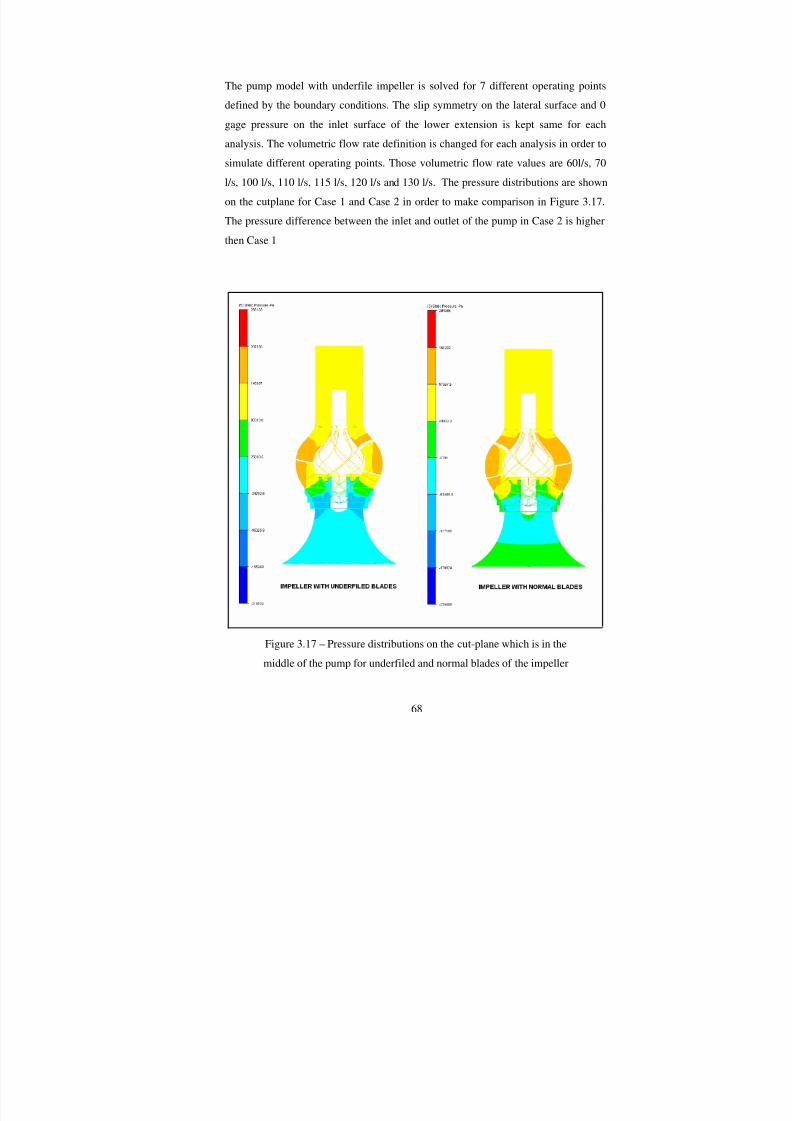
7/28/2019 design improvement of mixed flow pump through CFD.pdf
http://slidepdf.com/reader/full/design-improvement-of-mixed-flow-pump-through-cfdpdf 86/123
68
The pump model with underfile impeller is solved for 7 different operating points
defined by the boundary conditions. The slip symmetry on the lateral surface and 0
gage pressure on the inlet surface of the lower extension is kept same for each
analysis. The volumetric flow rate definition is changed for each analysis in order to
simulate different operating points. Those volumetric flow rate values are 60l/s, 70
l/s, 100 l/s, 110 l/s, 115 l/s, 120 l/s and 130 l/s. The pressure distributions are shown
on the cutplane for Case 1 and Case 2 in order to make comparison in Figure 3.17.
The pressure difference between the inlet and outlet of the pump in Case 2 is higher
then Case 1
Figure 3.17 – Pressure distributions on the cut-plane which is in the
middle of the pump for underfiled and normal blades of the impeller

7/28/2019 design improvement of mixed flow pump through CFD.pdf
http://slidepdf.com/reader/full/design-improvement-of-mixed-flow-pump-through-cfdpdf 87/123
69
The pump in Case 2 is also solved for 1450 rpm rotational speed of the impeller. The
volumetric flow rate of 30 l/s, 35 l/s, 50 l/s, 55 l/s and 60 l/s are defined in order to
simulate different operating points at 1450 rpm. Each analysis is run for 680
iterations and each analysis takes 42 hours for single operating point. The pressure
distributions on the impeller for both cases are shown in Figure 3.18. The pressure on
the underfiled blades is more uniformly distributed then the normal blade case.
Figure 3.18 – Pressure distributions on the impellers for normal and
underfiled cases.

7/28/2019 design improvement of mixed flow pump through CFD.pdf
http://slidepdf.com/reader/full/design-improvement-of-mixed-flow-pump-through-cfdpdf 88/123
7/28/2019 design improvement of mixed flow pump through CFD.pdf
http://slidepdf.com/reader/full/design-improvement-of-mixed-flow-pump-through-cfdpdf 89/123
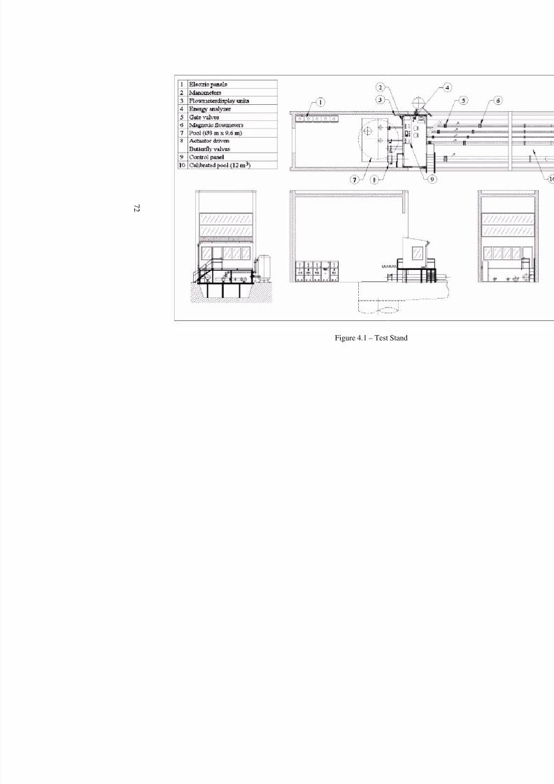
7/28/2019 design improvement of mixed flow pump through CFD.pdf
http://slidepdf.com/reader/full/design-improvement-of-mixed-flow-pump-through-cfdpdf 90/123
7 2
Figure 4.1 – Test Stand
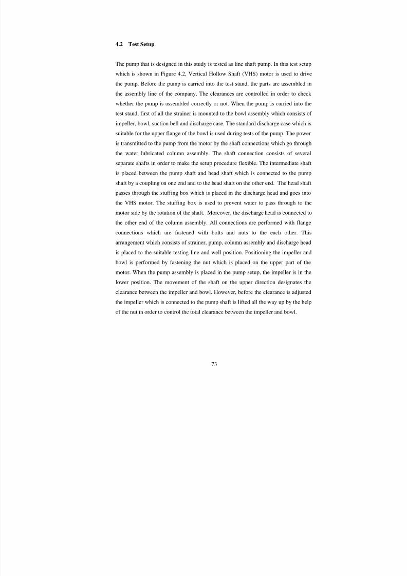
7/28/2019 design improvement of mixed flow pump through CFD.pdf
http://slidepdf.com/reader/full/design-improvement-of-mixed-flow-pump-through-cfdpdf 91/123

7/28/2019 design improvement of mixed flow pump through CFD.pdf
http://slidepdf.com/reader/full/design-improvement-of-mixed-flow-pump-through-cfdpdf 92/123
74
Figure 4.2 – In-line shaft Test Setup
4.3 Test Procedure and Data Processing
The test procedure given below is followed carefully in the pump performance tests.
Moreover the processing the data which is collected during the tests are also
explained after the test procedure is given.

7/28/2019 design improvement of mixed flow pump through CFD.pdf
http://slidepdf.com/reader/full/design-improvement-of-mixed-flow-pump-through-cfdpdf 93/123
75
4.3.1 Test Procedure
The procedure which is given below is followed during the pump tests performed in
this study.
1. The pump is assembled and prepared for the test.
2. Test setup is prepared and column assembly is filled with water.
3. The motor is connected to the suitable electrical panel by looking at the motor
electrical properties and the protection relay in the panel is set to the required
value by technician.
4. The protection relay is adjusted to the required value.
5. The rotation direction of the pump is checked and corrected by simply
starting the pump for a short period of time.
6. The connections to the butterfly valve from the intermediate pipe is
controlled and fastened in order to prevent the water leakage from the
connections.
7. The manometer and flowmeter are selected by looking at the maximum
expected head and flowrate of the pump to be tested respectively. The chosen
manometer is connected to the discharge pipe in the column assembly.Required valve configuration is set to direct the flow from collector pipe to
the chosen flowmeter.
8. Pump is started. If the frequency converter is used in order to operate the
pump at different speeds than the motor speed, the frequency is adjusted to
the desired working speed.

7/28/2019 design improvement of mixed flow pump through CFD.pdf
http://slidepdf.com/reader/full/design-improvement-of-mixed-flow-pump-through-cfdpdf 94/123
76
9. After the pump is started the exit pressure of the pump is adjusted by using
butterfly valve. When the pressure is in the desired level, no readings are
taken for a while before the pump reaches steady state operation at this point.
The decision of reaching the equilibrium is made by looking at the
oscillations on both flowmeter and manometer. When the oscillations damp
out, the recording is performed by means of flowrate and pressure readings
from the displays of flowmeter and manometer, respectively. The procedure
described above is repeated for a number of data points that are sufficient to
inspect the hydraulic and power consumption characteristics of the pump.
10. The pump is then stopped. The electrical connections are unplugged and the
safety regulations are followed to reassemble the pump from the test stand.
4.3.2 Processing the Test Data
The collected data from the pump test is processed by the following the procedure
given below to obtain the characteristics of the pump.
The instruments used during tests are periodically calibrated and calibration formulas
coming from the calibrations are used while processing the data. The calibration
results which are stated in the calibration reports are used to obtain these formulas
which have the data read as an input and the corresponding real value as an output.
Each recorded data are processed with the regarding formula of the instrument. Then
the calculations are performed as stated in the regarding standard, [22].
In order to find the total head of the pump, the velocity head is found as stated in the
regarding Reference 22. The velocity head is found simply dividing the flow rate to
the cross sectional area of the discharge pipe where the pressure is recorded at. The
nominal diameter is taken while calculating the cross sectional area of the discharge
pipe. The distance between the water level and the manometer location is added to

7/28/2019 design improvement of mixed flow pump through CFD.pdf
http://slidepdf.com/reader/full/design-improvement-of-mixed-flow-pump-through-cfdpdf 95/123
77
this value. The sum of these two is added to the pressure reading on the manometer
in order to get the pump head. These calculations are coming from the Bernoulli
equation written between points 1, 2 and 3 shown in the Figure 4.3.
Figure 4.3 – The points where the Bernoulli equation is written in order to find
the total head of the pump
7/28/2019 design improvement of mixed flow pump through CFD.pdf
http://slidepdf.com/reader/full/design-improvement-of-mixed-flow-pump-through-cfdpdf 96/123

7/28/2019 design improvement of mixed flow pump through CFD.pdf
http://slidepdf.com/reader/full/design-improvement-of-mixed-flow-pump-through-cfdpdf 97/123
79
The tests are performed with VHS type motor which has a nominal power of 22 kW.
The test results of impellers with normal and underfiled blades are given in Figure
4.4.
Figure 4.4 – Test Results with 22 kW motor for impellers with
normal and underfiled blades
The designed pump satisfies the tolerances given in the regarding standard [22], from
the design point of view for impeller with normal blades. The tolerances given in the
regarding standard, [22] are; ±8 % for the flow rate and ±5 % for the head of the
pump. In deed when the blades are underfiled, the best efficiency point moves
towards to the design point.

7/28/2019 design improvement of mixed flow pump through CFD.pdf
http://slidepdf.com/reader/full/design-improvement-of-mixed-flow-pump-through-cfdpdf 98/123
80
CHAPTER 5
RESULTS AND CONCLUSION
5.1 Discussion and Results
The discussions on the design, numerical experiments and tests are performed in this
chapter. The first part in this chapter is the discussion of the effects of the design
parameters on the hydraulic performance of the pump. The discussions on the CFD
analyses methodology are taken place after the discussions on the design. The lastpart is presenting comparisons of actual test results with CFD analyses results of the
designed pump.
In this thesis, a vertical turbine type mixed flow pump is designed, manufactured and
tested in Layne Bowler Pumps Company Inc. The CFD analyses are performed on
the designed pump and CFD results are compared with actual test results. The tests
of the pump are performed with an electric motor having the nominal speed of 1450rpm since suitable motor having 2900 rpm of rotational speed and required power
capacity is not found in the company during the testing period.
Since the design of the impeller is started with existing impeller layout, necessary
changes are made on this profile in order to meet the design point of the pump. The
methodology that is given in Chapter 2 regarding to the design of the impeller layout
is a trial and error procedure. In deed once the profile is constructed, the preliminary
design is performed and several points are checked in order to continue with shaping
the blades of the impeller. First check point is the blade number of the impeller. The
number of the blades with respect to the specific speed and the experience coming
from the company is followed while controlling the blade number. If the number of
blades that is found in the preliminary design are different then what is expected, the
geometrical change on the impeller layout is made. While making the geometrical
7/28/2019 design improvement of mixed flow pump through CFD.pdf
http://slidepdf.com/reader/full/design-improvement-of-mixed-flow-pump-through-cfdpdf 99/123
81
change, the static moment of the midstreamline is changed as the first case. Changing
the static moment of the midstreamline is made by increasing or reducing the length
of the midstreamline where the preliminary design is performed. If the number of
blades that are found in the preliminary design is higher then what is expected the
static moment of the midstreamline is decreased and if the number of the blades are
lower, the static moment is increased in order to satisfy the expectation. The main
reason of changing the characteristics of the midstreamline is coming from Equation
(2.39) and (2.40). If Equation (2.40) is put into Equation (2.39), the following
Equation is obtained.
)2
sin(..13 212
β β +=e
M z (5.1)
However while changing the static moment of midstreamline, the length of the
midstreamline is affected from this change. In order to minimize this change, the
midstreamline is moved diagonally in the 2D design plane to satisfy the desired
change on the blade number. If the blade number that is found in the preliminary
design is higher, the point of the midstreamline on the leading edge is extendedtowards the impeller inlet eye and the point of midstreamline on the trailing edge is
moved close to the rotating axis of the impeller. Moving the blade passage of the
impeller layout profile is simply positioning the blade passage close to the axis of
rotation of the impeller. Nevertheless if the blade number found in the preliminary
design is lower then what is expected, the reverse of this process is performed in
order to higher the blade number. The value of the blade number is tried to converge
to an integer value by applying these changes. It is found that the hydraulic
efficiency is highly affected by finding out the correct value of the blade number for
the desired characteristics of the pump.
Another important point for checking the conformity of impeller layout to the
expected design is the area distribution from leading edge to trailing edge of the
blade. The area distribution should be checked with two methods. The first one is

7/28/2019 design improvement of mixed flow pump through CFD.pdf
http://slidepdf.com/reader/full/design-improvement-of-mixed-flow-pump-through-cfdpdf 100/123
82
fitting the circles from inlet to outlet of the blade passage of the impeller layout.
Those circles are tangent to the hub and shroud profiles and the radius of the circles
should be changed well arranged from inlet breadth to the exit breadth. The second
method of controlling the area distribution is constructing the potential lines and
revolving these potential lines around the axis of rotation of the impeller. The ratio of
meridional velocities should be checked in order to attain better pump performance.
From the design experience, the ratio of Vm0 /Vm1 is between 0.85 - 1 and the ratio of
Vm2 /Vm1 is between 0.6 - 0.75. However while calculating these ratios, the blade
thickness should be considered.
The blade thickness of the impeller is directly affecting the hydraulic performance of
the pump. However from the production point of view the blade thickness is selected
according to the casting capabilities. Although the meat thicknesses of the impeller
should be selected close to the thickness of the blade in order to cast the impeller
properly.
The degree of reaction is defined as the ratio between the pressure head of the pump,
Hp and the theoretical head of the pump, Hth. The degree of reaction of the pump thatis designed in this study is 0.74 if the midstreamline is taken into account for
calculations. On the other hand when the degrees of reaction for the other streamlines
are calculated, the values lie between 0.6 and 0.8, from hub to shroud respectively.
The degree of reaction represents the characteristics of the pump. It is stated in
Reference [1] that, higher the degree of reaction, the greater the specific speed of the
pump. Hence the rotodynamic pump that is designed in this study is a reaction
machine.
Pfleiderer’s correction factor, Cp is stated to be between 0.25 and 0.35 in preliminary
design part of Chapter 2. It is found that Cp is 0.29 for midstreamline. The Cp value
is between 0.2 and 0.4 for the other streamlines and Cp value is gradually increasing
from hub to shroud. The Pfleiderer’s correction factor approach is applicable for the
pump that is designed in this study.

7/28/2019 design improvement of mixed flow pump through CFD.pdf
http://slidepdf.com/reader/full/design-improvement-of-mixed-flow-pump-through-cfdpdf 101/123
83
While applying numerical experimentation on the designed pump several points
should be carefully followed. The first point is selecting the boundary conditions.
Defining volumetric flow rate boundary condition to the exit and pressure boundary
condition to the inlet of the pump is used in the CFD analyses. These boundary
condition definitions are found to be useful while using CFdesign in order to have
faster convergence than defining pressure-pressure and volumetric flow rate-
volumetric flow rate boundary conditions to the inlet and exit respectively.
The CFD solutions are affected by the quality of generated elements that are forming
the solution domain inside the pump. While defining the size of the meshes that are
generated for the solution, rotating region and impeller should be meshed with
smaller elements then the other parts. However the element size is increased
gradually for the other parts in order to keep the aspect ratio as low as possible.
When convergence is followed by checking the physical quantities such as pressure
and velocity components from different cut-planes at the inlet and outlet of the
pump, the oscillations may be investigated. If the oscillations are investigated, the
aspect ratio should be checked. The regions having higher aspect ratio should be re-
meshed and the aspect ratio is tried to be minimized. It is also found that if theextensions at the inlet and outlet of the pump are not long enough the solutions may
diverge. Total number of fluid elements that are generated in pump applications
around 1.5 million give reliable results when they are compared with actual test
results.
The time step size is the parameter which defines the rotation of the machine in
degrees per time step, [13]. When the time step size is adjusted for three degrees of rotation of the machine, in this case the impeller, the results converges slower but the
reliable results are investigated.
CFdesign calculates the hydraulic torque on the impeller which is surrounded by the
rotating region. This torque value is used to calculate the hydraulic efficiency of the
pump that is designed in this study. In order to calculate the pump efficiency, the

7/28/2019 design improvement of mixed flow pump through CFD.pdf
http://slidepdf.com/reader/full/design-improvement-of-mixed-flow-pump-through-cfdpdf 102/123
84
hydraulic efficiency should be multiplied by the volumetric efficiency and the
mechanical efficiency. Since the leakage region between the impeller and bowl is
very small compare to the other water passages inside the pump, it is difficult to
generate meshes in this region. The difficulty of putting meshes is mainly caused by
hardware capabilities. CFD software has an automatic mesh generator and when the
user tries to put small size meshes in leakage paths, the total amount of mesh
generated in the analysis increases more than the 32 bit environment can handle.
Nevertheless the analyses are tried to be performed with a workstation which has 2
XEON 64 bit 3.4 GHz processor, 4 GB of RAM and installed 64 bit Windows
operating system. However the both the 64 bit Cfdesign V.8 which is a beta version
and 32 bit Cfdesign did not work properly in 64 bit environment. On the other hand it
is investigated that more elements are generated with meshing the gaps between
stator and rotor in 64 bit environment. The volumetric efficiency is taken as the
assumption that is made in Chapter 2 as 96% while calculating the pump efficiency.
The mechanical efficiency is also taken as the design value which is 96% percent
during pump efficiency calculation. However in order to make comparison between
the CFD results and test results the motor efficiency should also be estimated. The
motor efficiencies are taken from the motor manufacturers catalogues in order tocalculate pump efficiency. The values of the efficiencies of the motors are based on
the catalogue values of the motor manufacturer, [23]. Since the pump is solved for
single stage in CFD, the head rise that is calculated in the analysis is multiplied by 4
in order to compare the results with actual test results.
The comparison of CFD results which are solved for 1450 rpm of rotational speed of
the impeller with actual test results performed with 22 kW motor is given in Figure5.1 and Figure 5.2. The CFD results by means of head and efficiency characteristics
are within the tolerance limits given in the regarding standard, [22].

7/28/2019 design improvement of mixed flow pump through CFD.pdf
http://slidepdf.com/reader/full/design-improvement-of-mixed-flow-pump-through-cfdpdf 103/123
85
Figure 5.1 – Test results with 22 kW motor and CFD results by means of head
versus flow rate and system efficiency versus flow rate
The underfiling is performed in the machine shop with a similar method that is
modelled in CAD environment. However it is hard to process the same metal
removal that is done in CAD due to manufacturing capabilities.
The assumptions for the volumetric and mechanical efficiencies are also the cause of
the errors during the calculations. Improving the hardware of the computers used
during the analyses may give the ability to calculate the volumetric efficiency.
However from the industrial point of view the CFD results satisfy the needs of the
company. In order to control the mechanical efficiency, the pump should be carefully
assembled. The manufacturing tolerances should strictly be followed in order not to
have wear between the rotating and stationary elements especially in the bearings in
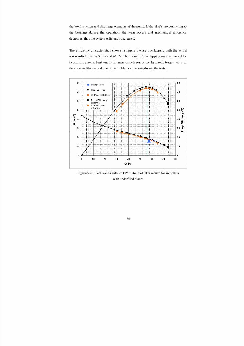
7/28/2019 design improvement of mixed flow pump through CFD.pdf
http://slidepdf.com/reader/full/design-improvement-of-mixed-flow-pump-through-cfdpdf 104/123
86
the bowl, suction and discharge elements of the pump. If the shafts are contacting to
the bearings during the operation, the wear occurs and mechanical efficiency
decreases, thus the system efficiency decreases.
The efficiency characteristics shown in Figure 5.6 are overlapping with the actual
test results between 50 l/s and 60 l/s. The reason of overlapping may be caused by
two main reasons. First one is the miss calculation of the hydraulic torque value of
the code and the second one is the problems occurring during the tests.
Figure 5.2 – Test results with 22 kW motor and CFD results for impellers
with underfiled blades

7/28/2019 design improvement of mixed flow pump through CFD.pdf
http://slidepdf.com/reader/full/design-improvement-of-mixed-flow-pump-through-cfdpdf 105/123

7/28/2019 design improvement of mixed flow pump through CFD.pdf
http://slidepdf.com/reader/full/design-improvement-of-mixed-flow-pump-through-cfdpdf 106/123
88
Figure 5.3 – Test results with 22 kW motor converted to 2900 rpm and CFD results
The conversion calculations using Equation (5.4) showed that the design point is
satisfied within the given tolerance limits in the regarding reference, [22]. However
performing the actual tests with a 2900 rpm electric motor gives more reliable results
then converting the 1450 rpm test results to 2900 rpm by using the formula.
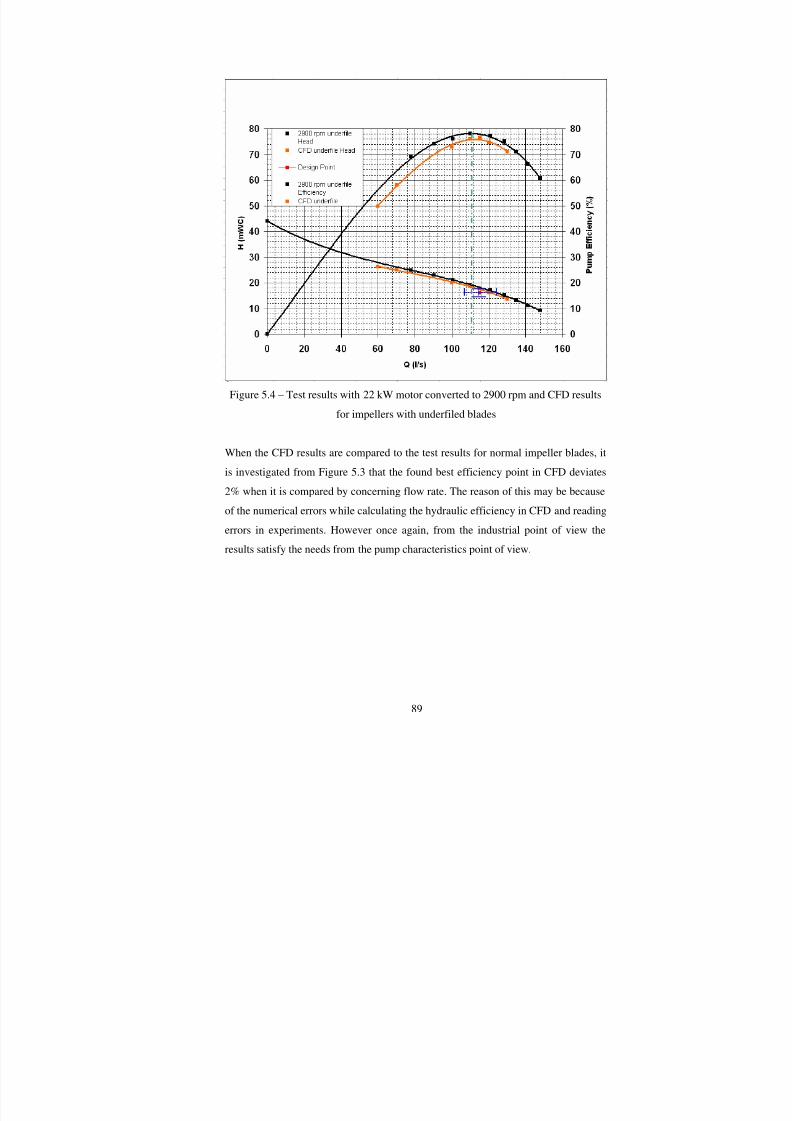
7/28/2019 design improvement of mixed flow pump through CFD.pdf
http://slidepdf.com/reader/full/design-improvement-of-mixed-flow-pump-through-cfdpdf 107/123
89
Figure 5.4 – Test results with 22 kW motor converted to 2900 rpm and CFD results
for impellers with underfiled blades
When the CFD results are compared to the test results for normal impeller blades, it
is investigated from Figure 5.3 that the found best efficiency point in CFD deviates
2% when it is compared by concerning flow rate. The reason of this may be because
of the numerical errors while calculating the hydraulic efficiency in CFD and reading
errors in experiments. However once again, from the industrial point of view the
results satisfy the needs from the pump characteristics point of view.
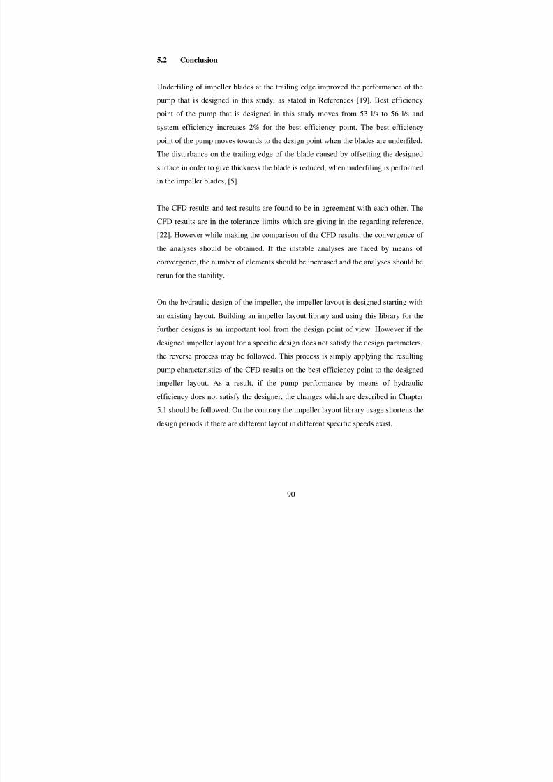
7/28/2019 design improvement of mixed flow pump through CFD.pdf
http://slidepdf.com/reader/full/design-improvement-of-mixed-flow-pump-through-cfdpdf 108/123
7/28/2019 design improvement of mixed flow pump through CFD.pdf
http://slidepdf.com/reader/full/design-improvement-of-mixed-flow-pump-through-cfdpdf 109/123
91
The design of the pumps still depends on the experience of the designer. However
using CFD software which is integrated into the design procedure allows the
designers to better understand the flow physics inside the pumps. The integration of
the CFD software to the design process is a continuous procedure. The code should
be verified in each case study by comparing the CFD results with actual test results.
The manufacturing of the pump is important as the hydraulic design studies and
numerical experimentations. While producing the pump, the cores and core boxes
should be manufactured by following the original design. However, the designs
should be robust in order to manufacture the pumps easily and getting the closest
pump characteristics when the test results are compared with the CFD results and
hydraulic design of the pump. Selecting the suitable blade and vane thicknesses,
blade swirl and vane swept angles are important from the manufacturing point of
view.
5.3 Future Work
In order to improve the design procedure that is followed in this thesis, there areseveral point may be checked. The pressure distribution may be determined on the
designed streamlines by using CFD. The plots of the pressure distribution versus
meridional distance on the pressure and suction sides of the impeller blade give an
idea about the theoretical head of the pump that is aimed to be designed. Moreover,
the distribution of the velocity components on the designed streamlines may be
drawn by the help of CFD and these distributions can be compared with the velocity
distributions on the shaping of the blades part of the design.
The computerized design codes such as CFTurbo, Concepts-NREC’s Pumpal, PDC
by Hans Spring and TurboDesign-1 may be integrated into the design process of the
pumps in order to shorten the design periods. However it is kept in mind those codes
should be verified with the theoretical calculations on the design procedure and
should be used as a tool in the design

7/28/2019 design improvement of mixed flow pump through CFD.pdf
http://slidepdf.com/reader/full/design-improvement-of-mixed-flow-pump-through-cfdpdf 110/123
92
The CFD analyses are performed for whole pump in this study. However blade top
blade analysis may be performed for the impeller after the design of the impeller is
completed. However in order to perform CFD analysis to the single flow passage
which is between two adjacent blades, the stacking of the blade at the trailing edge
should be uniform. The reason of this uniformity is because of the volumes that are
added to the inlet and exit of the impeller. If the impeller leading edge is not
uniformly shaped between the hub and shroud, it is hard to assemble the exit volume
to the impeller exit for the blade to blade analysis. If the blade to blade analysis is
performed the periodic boundary conditions are used and the analyses are run in
steady state form. This procedure shortens the analysis run time and allows the
designer to investigate the flow structure inside the single flow passage of the
impeller. Nevertheless the pressure distribution is investigated and the design may be
improved in order to achieve the desired head of the pump.
If the software that is used in this thesis can handle 64 bit environment solutions
properly by means of convergence, the pump analysis may be performed by
generating elements to the gaps between the stator and rotor where the volumetric
leakage occurs.
From the production point of view, the casting technique that is used to cast the
products in this study is simple gravity die casting. In this method, the thicknesses
that could be cast are limited. However using another casting techniques such as
investments casting may allow the designs to be cast with smaller thicknesses.
Decreasing the thickness of the blade increases the pump performance. However,
decreasing the thicknesses of the blades allows the impellers face with wear whenthey are operating in environments where the impurities exist in the working fluid
such as sand. The thicknesses should be adjusted by considering the overall operating
life of the pumps.

7/28/2019 design improvement of mixed flow pump through CFD.pdf
http://slidepdf.com/reader/full/design-improvement-of-mixed-flow-pump-through-cfdpdf 111/123
93
REFERENCES
1. Lazarkiewicz, S. and Troskolanski, A. T. (1965) Impeller Pumps, PergamonPress Ltd., Oxford.
2. Aksel, M. H. (1999) Fluid Mechanics, Middle East Technical University,Ankara.
3. Dicmas, J. L. (1987) Vertical Turbine, Mixed Flow, and Propeller Pumps,McGraw – Hill Inc., U.S.A.
4. Anderson, H. H. (1986) Submersible Pumps and Their Applications, 1st Ed , The
Trade and Technical Press Limited, England.
5. Stepanoff, A. J. (1957) Flow Pumps Design, and Application, John Wiley &Sons Inc., U.S.A.
6. Sayers, A. T. (1990) Hydraulic and compressible flow turbomachines,McGraw-Hill Book Company, England.
7. Wendt J. F. (1992) Computational Fluid Dynamics: an Introduction, 1st Ed ,Springer-Verlag., New York U.S.A.
8. Goto, A., Nohmi, M., Sakurai, T. and Sogawa, Y., (2002) “ Hydrodynamic Design System for Pumps Based on 3-D CAD, CFD, and Inverse Design Method ”, ASME Journal of Fluids Engineering Vol.124 pp. 329-335.
9. Walker, P. J. and Dawes, W. N., (1990) “The Extension and Application of Three-Dimensional Time-Marching Analysis to IncompressibleTurbomachinery Flows,” ASME Journal of Turbomachinery., Vol. 112, pp.385-390.
10. Goto, A. (1995) “ Numerical and Experimental Study of 3-D Flow Fields withina Diffuser Pump Stage at Off-Design Condition,” ASME Fluids 95, FED-Vol.227, pp. 1-9.
11. CFX User Manual Version 5.6 (2003) CFX Ltd., United Kingdom.
12. Muggli, F. A., Holbein, P. and Dupont, P., (2002) “CFD Calculation of a Mixed Flow Pump Characteristics from Shutoff to Maximum Flow” ASMEJournal of Fluids Engineering., Vol. 124, pp. 798-802.

7/28/2019 design improvement of mixed flow pump through CFD.pdf
http://slidepdf.com/reader/full/design-improvement-of-mixed-flow-pump-through-cfdpdf 112/123

7/28/2019 design improvement of mixed flow pump through CFD.pdf
http://slidepdf.com/reader/full/design-improvement-of-mixed-flow-pump-through-cfdpdf 113/123
95
APPENDIX A
Figure A.1 – Photograph of impeller core and core box
Figure A.2 – Photograph of bowl core and core box

7/28/2019 design improvement of mixed flow pump through CFD.pdf
http://slidepdf.com/reader/full/design-improvement-of-mixed-flow-pump-through-cfdpdf 114/123
96
Figure A.3 – Photograph of impeller before machining
Figure A.4 – Photograph of impeller after machining

7/28/2019 design improvement of mixed flow pump through CFD.pdf
http://slidepdf.com/reader/full/design-improvement-of-mixed-flow-pump-through-cfdpdf 115/123
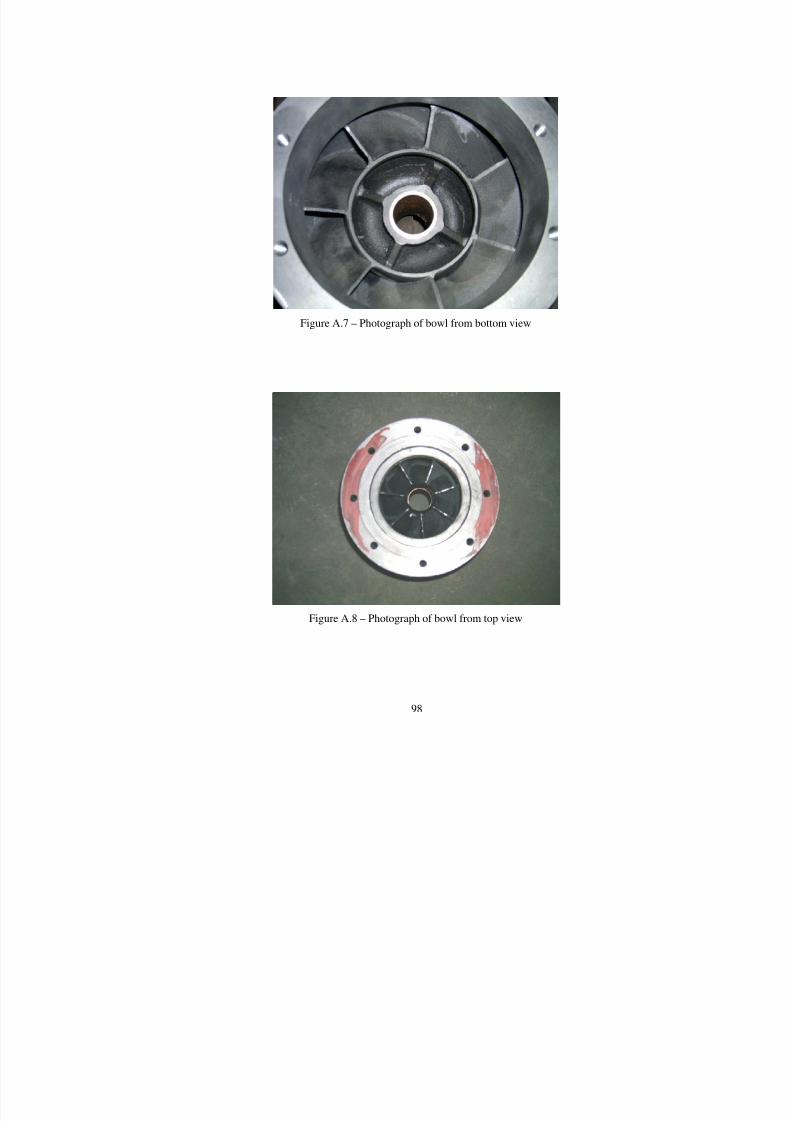
7/28/2019 design improvement of mixed flow pump through CFD.pdf
http://slidepdf.com/reader/full/design-improvement-of-mixed-flow-pump-through-cfdpdf 116/123
98
Figure A.7 – Photograph of bowl from bottom view
Figure A.8 – Photograph of bowl from top view
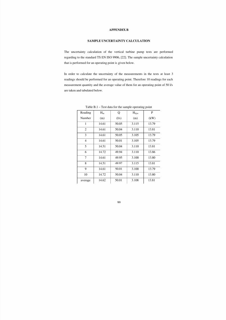
7/28/2019 design improvement of mixed flow pump through CFD.pdf
http://slidepdf.com/reader/full/design-improvement-of-mixed-flow-pump-through-cfdpdf 117/123
99
APPENDIX B
SAMPLE UNCERTAINTY CALCULATION
The uncertainty calculation of the vertical turbine pump tests are performed
regarding to the standard TS EN ISO 9906, [22]. The sample uncertainty calculation
that is performed for an operating point is given below.
In order to calculate the uncertainty of the measurements in the tests at least 3
readings should be performed for an operating point. Therefore 10 readings for eachmeasurement quantity and the average value of them for an operating point of 50 l/s
are taken and tabulated below.
Table B.1 – Test data for the sample operating point
Reading
Number
Hm
(m)
Q
(l/s)
Hdyn
(m)
P
(kW)1 14.61 50.05 3.115 13.79
2 14.61 50.04 3.110 13.81
3 14.61 50.05 3.105 13.79
4 14.61 50.01 3.105 13.79
5 14.51 50.04 3.110 13.81
6 14.72 49.94 3.110 13.86
7 14.61 49.95 3.100 13.808 14.51 49.97 3.115 13.81
9 14.61 50.01 3.100 13.79
10 14.72 50.04 3.110 13.80
average 14.62 50.01 3.108 13.81

7/28/2019 design improvement of mixed flow pump through CFD.pdf
http://slidepdf.com/reader/full/design-improvement-of-mixed-flow-pump-through-cfdpdf 118/123
100
The total uncertainty of a measurement, UT, is composed of systematic and random
uncertainties that are represented by US and UR respectively and the formula is given
for UT is given by:
22
RS T U U U += (B.1)
The random uncertainty of a measurement is defined as two times the standard
deviation of it in the regarding standard, [22]. The standard deviation is calculated in
order to find out the random uncertainties of each measurement by the formula given
as:
n
x x x x x xs n
222
21 )(...)()( −++−+−
= (B.2)
Where x is the average value of the measurement, x1, x2, x3, …, xn are the
measurement values and n is the total number of measurements. The standard
deviation, the absolute value and the normalized value of the uncertainties are
tabulated below for each measurement quantity.
Table B.2 – Values for standard deviation and random uncertainty for
each measured quantity.
Hm
(m)
Q
(l/s)
Hdyn
(m)
P
(kW)
Standard
deviation0.065 0.040 0.005 0.020
Absolute random
Uncertainty0.130 0.080 0.010 0.040
Random Uncertainty (%) 0.884 0.160 0.328 0.292

7/28/2019 design improvement of mixed flow pump through CFD.pdf
http://slidepdf.com/reader/full/design-improvement-of-mixed-flow-pump-through-cfdpdf 119/123
101
The systematic uncertainty is defined as the sensitivity of the instrument or method
used for measuring and constant during the measurements, [22]. The calibration
certificates of each instrument that are used during the tests are used to define the
systematic uncertainties for each measured quantity.
Table B.3 – Values of systematic uncertainty for each measured quantity
Hm
(%)
Q
(%)
Hdyn
(%)
P
(%)
2.85 0.70 0.01 1.33
The total uncertainty of each measured quantity is calculated by using the values in
Table B.3, B.2 and formula given in Equation (B.1). The results are tabulated below
in Table (B.4).
Table B.4 – Values of total uncertainty for each measured quantityHm
(%)
Q
(%)
Hdyn
(%)
P
(%)
2.98 0.72 0.33 1.36
The total head of the pump, Ht, is calculated by the formula given below.
g
V H H H f
dynmt .2
2
++= (B.3)
Where Hm is the manometric head, Hdyn is the dynamic water level as described in
Chapter 4 and Vf is the velocity of the pumping fluid where the pressure reading is
performed. In this case Vf is found by dividing the measured flow rate to the cross-

7/28/2019 design improvement of mixed flow pump through CFD.pdf
http://slidepdf.com/reader/full/design-improvement-of-mixed-flow-pump-through-cfdpdf 120/123
102
section area, Ap, of the pipe where the pressure reading is performed from. The
regarding formula is given below.
p
f A
QV = (B.4)
The total uncertainty of Vf , UT_f is calculated using the nominal diameter of the pipe
which is 0.018 m2 and the formula given below:
QT
p
f T U
A
U __ .1
= (B.5)
Where, UT_Q is the total absolute uncertainty for the flow rate. If the values are
substitutes into Equation (B.5):
00036.00018.0
1_ xU f T =
020.0_ ±= f T U m/s
The total uncertainty of the total head, UT_Ht is calculated the formula given below:
2_
2
_
2
__ ).( Vf T
f
HdynT HmT Ht T U g
V U U U ++±= (B.6)
Substituting the absolute values for each total uncertainty into Equation (B.6), UT_Ht
is calculated as:
222_ )02.0
81.9
83.2(01.0436.0 xU Ht T ++±=

7/28/2019 design improvement of mixed flow pump through CFD.pdf
http://slidepdf.com/reader/full/design-improvement-of-mixed-flow-pump-through-cfdpdf 121/123

7/28/2019 design improvement of mixed flow pump through CFD.pdf
http://slidepdf.com/reader/full/design-improvement-of-mixed-flow-pump-through-cfdpdf 122/123
104
23
3
25_ )102
10
1()101( −
−
− +±= x x xU T ρ
2_ ±= ρ T U kg/m3
The total uncertainty of the system efficiency, UT_ηs which is also defined as wire to
water efficiency is derived from Equation (B.7) as given below:
+
+
+
=PT
t
Ht T QT t
T t
sT
U P
H Qg
U P
QgU
P
H gU
P
H Qg
U _2
___
_
....
...
...
...
ρ
ρ ρ ρ
η (B.10)
If the regarding values are substituted into Equation (B.10):
+
+
+
=2
2
2
22
_
188.013810
13.1881.9100044.013810
050.081.91000
00036.013810
13.1881.910002
13810
13.18050.081.9
x x x x x x
x x x
x x x
U sT η
64.1_ ±=sT U η %
The total uncertainty for the wire to water efficiency is normalized by dividing 1.64
% to the wire to water efficiency at the operating point and the value is found to be
2.55 %.
The results are tabulated below for the uncertainty analysis and compared with the
given standard limits for TS EN ISO 9906, [22]. While making the calculations for
the density of the fluid, the density is taken to be constant through out the
experiments.
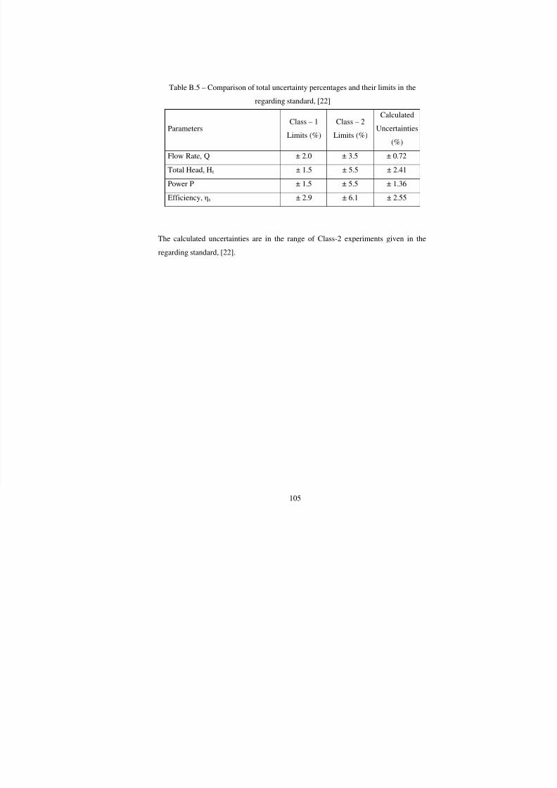
7/28/2019 design improvement of mixed flow pump through CFD.pdf
http://slidepdf.com/reader/full/design-improvement-of-mixed-flow-pump-through-cfdpdf 123/123
Table B.5 – Comparison of total uncertainty percentages and their limits in the
regarding standard, [22]
ParametersClass – 1
Limits (%)
Class – 2
Limits (%)
Calculated
Uncertainties
(%)
Flow Rate, Q ± 2.0 ± 3.5 ± 0.72
Total Head, Ht ± 1.5 ± 5.5 ± 2.41
Power P ± 1.5 ± 5.5 ± 1.36
Efficiency, ηs ± 2.9 ± 6.1 ± 2.55
The calculated uncertainties are in the range of Class-2 experiments given in the
regarding standard, [22].