design exploration with ansys v12: the response surface method · design exploration with ansys...

© 2009 ANSYS, Inc. All rights reserved. 1 ANSYS, Inc. Proprietary

Design Exploration with ANSYS V12: The response surface methodStep by step Structural Mechanics example

Design Exploration with ANSYS V12: The response surface methodStep by step Structural Mechanics example

An ANSYS TutorialAn ANSYS Tutorial


Analysis modelAnalysis model


Finding a good design

• In this introduction to DesignXplorer, we will use the parametric features of ANSYS Workbench to find a satisfying design for a hook.

• The hook (see following slide for geometry) should :– withstand a load of 6000N – the maximum stress should not exceed the

yield stress;– be robust enough so as to resist scattering of the load and unavoidable

variations of its dimensions (manufacturing variations…);– And of course, its weight must be as low as possible.

• To reach our goal, we will use a DOE analysis: parameters are varied continuously over given ranges and the performance of the hook is examined over these ranges. Some possible candidates for best design will be determined.


Hook geometry

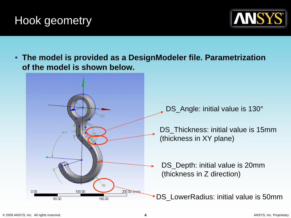
• The model is provided as a DesignModeler file. Parametrizationof the model is shown below.

DS_Angle: initial value is 130°

DS_Thickness: initial value is 15mm (thickness in XY plane)

DS_LowerRadius: initial value is 50mm

DS_Depth: initial value is 20mm(thickness in Z direction)


Simulation environment

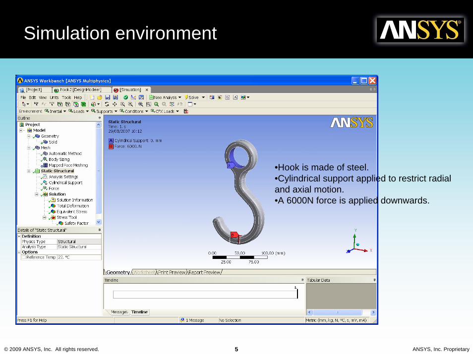
•Hook is made of steel.•Cylindrical support applied to restrict radial and axial motion.•A 6000N force is applied downwards.


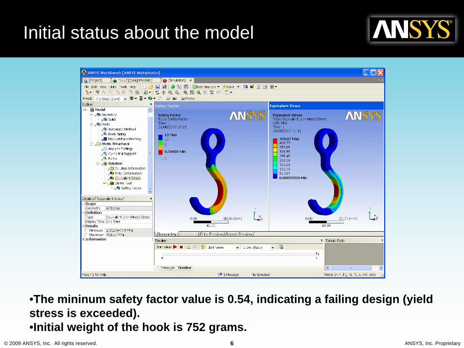
Initial status about the model

•The mininum safety factor value is 0.54, indicating a failing design (yieldstress is exceeded).•Initial weight of the hook is 752 grams.


Defining the parametric simulation model with ANSYS WorkbenchDefining the parametric simulation model with ANSYS Workbench


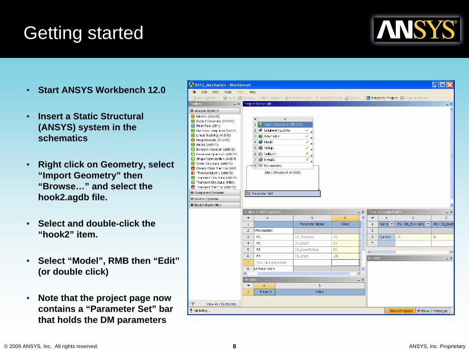
Getting started

• Start ANSYS Workbench 12.0

• Insert a Static Structural (ANSYS) system in the schematics

• Right click on Geometry, select “Import Geometry” then “Browse…” and select the hook2.agdb file.

• Select and double-click the “hook2” item.

• Select “Model”, RMB then “Edit”(or double click)

• Note that the project page now contains a “Parameter Set” bar that holds the DM parameters


A note on geometric parameter

• In this examples, the geometric parameters are defined from ANSYS DesignModeler and are automatically collected in the parameter set – regardless of their names. If some of them are not required for a parametric analysis, simply deactivate them.

• Geometric parameters can also be defined directly from your CAD system – using a prefix to flag the ones that are relevant for the simulation.

• You can also mix parameter sources: some could be imported from the CAD model and additional ones defined in ANSYS DesignModeler.


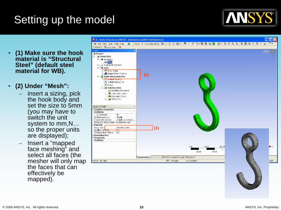
Setting up the model

• (1) Make sure the hook material is “Structural Steel” (default steel material for WB).

• (2) Under “Mesh”:– insert a sizing, pick

the hook body and set the size to 5mm (you may have to switch the unit system to mm,N…so the proper units are displayed);

– Insert a “mapped face meshing” and select all faces (the mesher will only map the faces that can effectively be mapped).

(1)

(2)


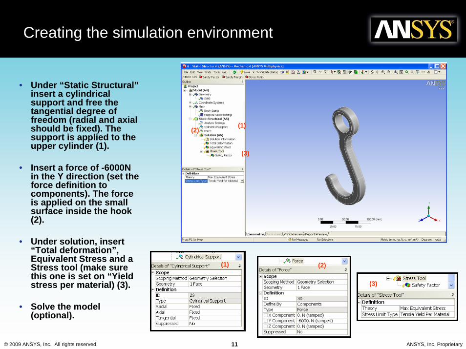
Creating the simulation environment

• Under “Static Structural”insert a cylindrical support and free the tangential degree of freedom (radial and axial should be fixed). The support is applied to the upper cylinder (1).

• Insert a force of -6000N in the Y direction (set the force definition to components). The force is applied on the small surface inside the hook (2).

• Under solution, insert “Total deformation”, Equivalent Stress and a Stress tool (make sure this one is set on “Yield stress per material) (3).

• Solve the model (optional).

(1)(2)

(3)

(2)(1)

(3)


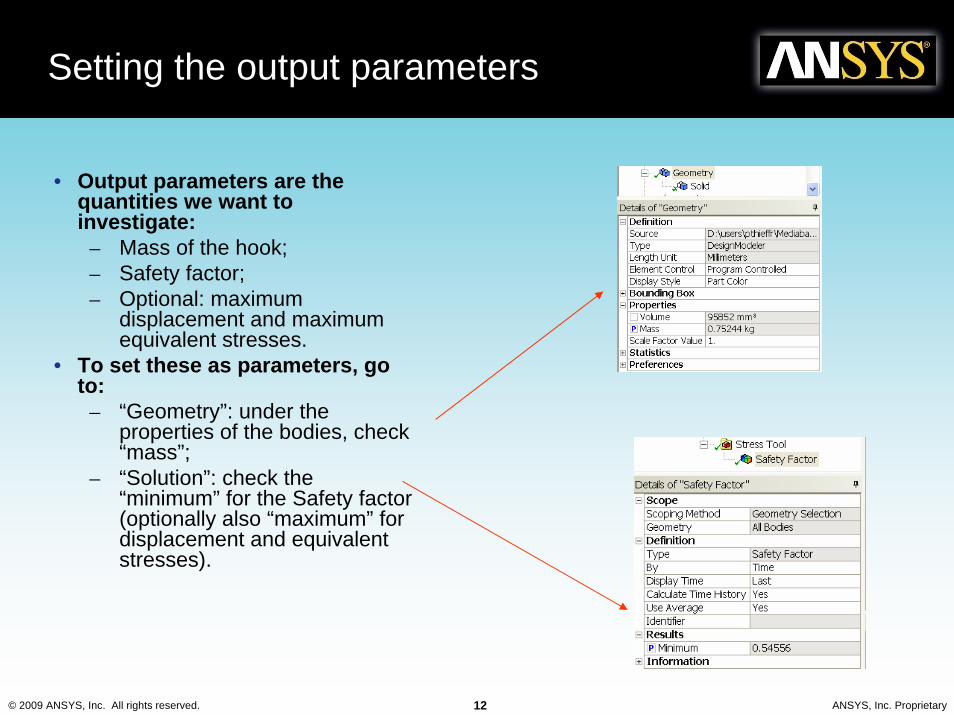
Setting the output parameters

• Output parameters are the quantities we want to investigate:

– Mass of the hook;– Safety factor;– Optional: maximum

displacement and maximum equivalent stresses.

• To set these as parameters, go to:

– “Geometry”: under the properties of the bodies, check “mass”;

– “Solution”: check the “minimum” for the Safety factor (optionally also “maximum” for displacement and equivalent stresses).


A note on parameters

• ANSYS Workbench allows to create parameters from most of the items in the simulation tree:– Material properties– Contacts – Loads– Boundary conditions– Results

• If you are using APDL code in the Mechanical Simulation Environment:– the input arguments (arg0 to arg9) can be parameterized– The output (for post-processing operations) can be exposed as

output parameters


Save your project

• In the file menu, select “Save Project”.


Response surface modeling and optimizationResponse surface modeling and optimization


Principles

• What is the Response Surface method:– Based on the number of input parameters (ANSYS Workbench -

Simulation, CAD, etc.), a given number of solutions (design points) are required to build a response surface;

– A Design of Experiments, or DOE, method determines how many and which design points should be solved;

– Once the required solutions are complete a response surface is fitted through the results allowing designs to be queried where no “hard” solution exists.

• Rather than providing values for discrete sets of parameters, the Response Surface provides a continuous variation of the output quantities with respect to the input parameters.


Parametric variations for the hook

• We are going to perform the deterministic analysis of the hook for the following parameter ranges:– DS_Thickness: 15mm to 25mm– DS_Depth: 15mm to 25mm– DS_LowerRadius: 45mm to 55mm– DS_Angle: 120° to 150°

• We do not need to specify how many points are to be taken for each parameter: the DOE method will give us the necessary points.

• Also, after performing the analysis, we will be able to give an estimate of the output parameters for ANY value of the 4 parameters (between their min and max values).


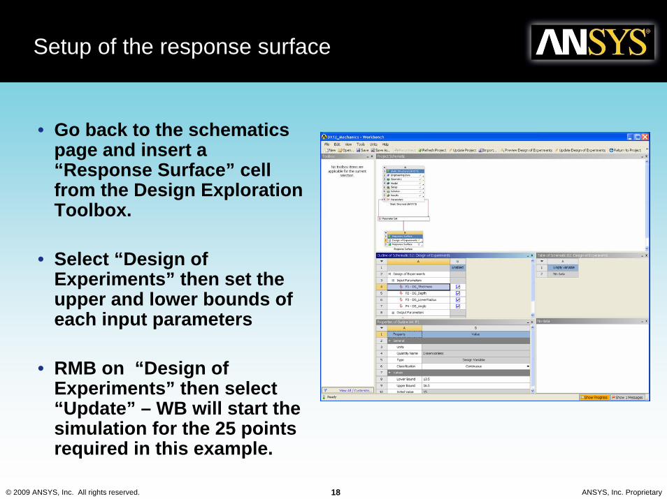
Setup of the response surface

• Go back to the schematics page and insert a “Response Surface” cell from the Design Exploration Toolbox.

• Select “Design of Experiments” then set the upper and lower bounds of each input parameters

• RMB on “Design of Experiments” then select “Update” – WB will start the simulation for the 25 points required in this example.


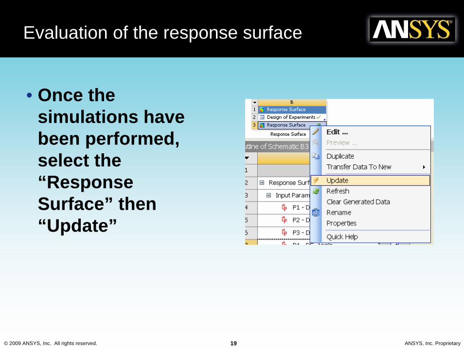
Evaluation of the response surface

• Once the simulations have been performed, select the “Response Surface” then “Update”


Understanding the results

• Once the response surfaces have been built, several tools are available to investigate the model:– Min/max search;– Surface plots;– XY plots;– Sensitivities;– Optimization and trade-off plots.


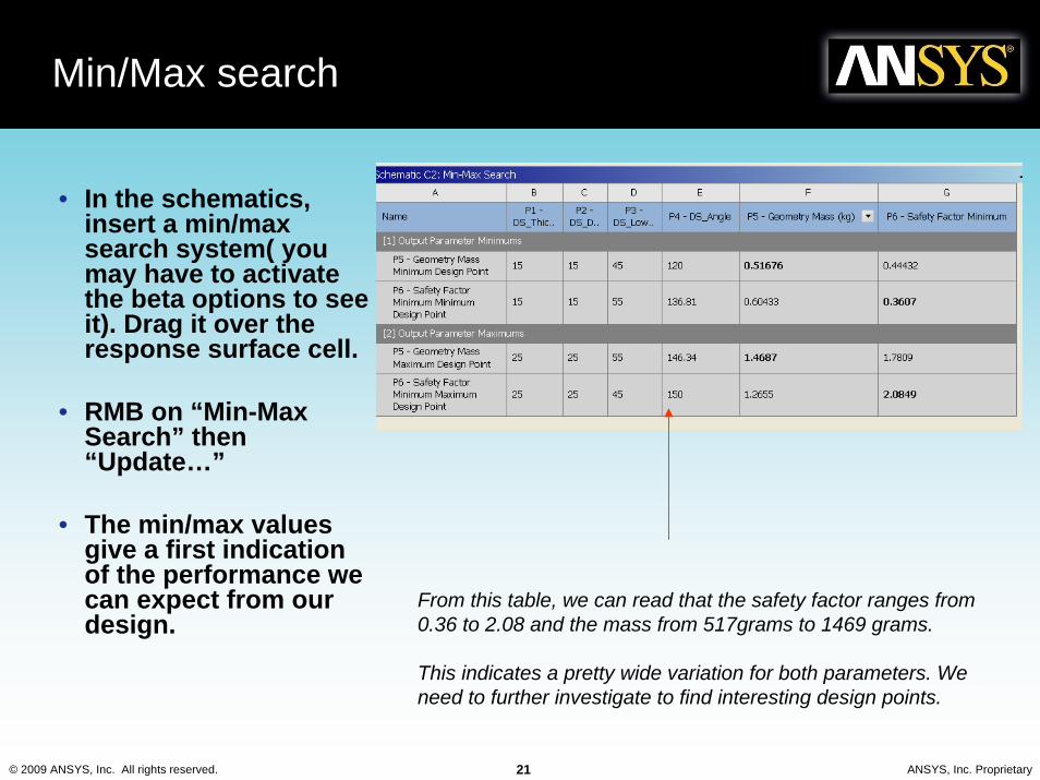
Min/Max search

• In the schematics, insert a min/max search system( you may have to activate the beta options to see it). Drag it over the response surface cell.

• RMB on “Min-Max Search” then “Update…”

• The min/max values give a first indication of the performance we can expect from our design.

From this table, we can read that the safety factor ranges from 0.36 to 2.08 and the mass from 517grams to 1469 grams.

This indicates a pretty wide variation for both parameters. We need to further investigate to find interesting design points.


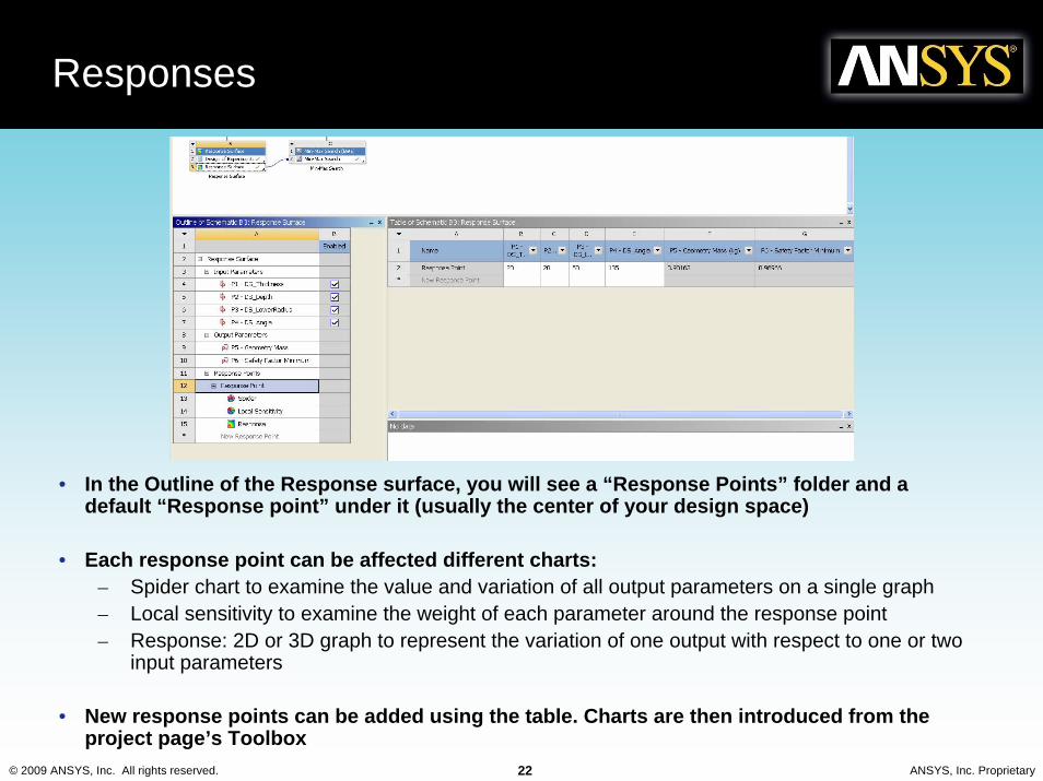
Responses

• In the Outline of the Response surface, you will see a “Response Points” folder and a default “Response point” under it (usually the center of your design space)

• Each response point can be affected different charts:– Spider chart to examine the value and variation of all output parameters on a single graph– Local sensitivity to examine the weight of each parameter around the response point– Response: 2D or 3D graph to represent the variation of one output with respect to one or two

input parameters

• New response points can be added using the table. Charts are then introduced from the project page’s Toolbox


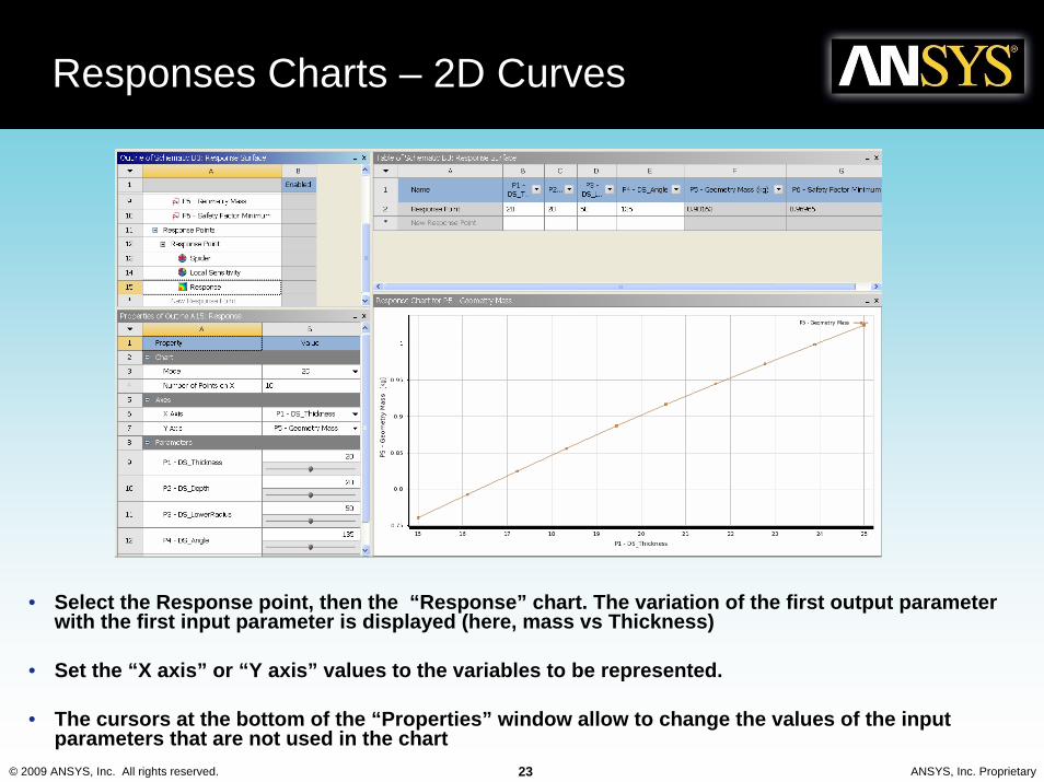
Responses Charts – 2D Curves

• Select the Response point, then the “Response” chart. The variation of the first output parameter with the first input parameter is displayed (here, mass vs Thickness)

• Set the “X axis” or “Y axis” values to the variables to be represented.

• The cursors at the bottom of the “Properties” window allow to change the values of the input parameters that are not used in the chart


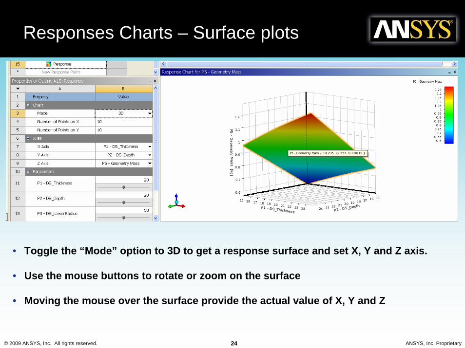
Responses Charts – Surface plots

• Toggle the “Mode” option to 3D to get a response surface and set X, Y and Z axis.

• Use the mouse buttons to rotate or zoom on the surface

• Moving the mouse over the surface provide the actual value of X, Y and Z


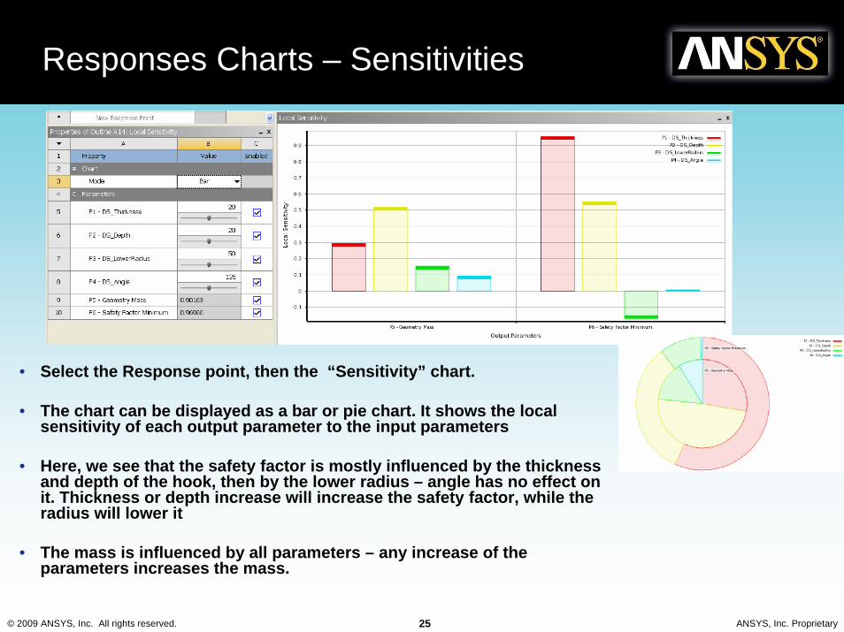
Responses Charts – Sensitivities

• Select the Response point, then the “Sensitivity” chart.

• The chart can be displayed as a bar or pie chart. It shows the local sensitivity of each output parameter to the input parameters

• Here, we see that the safety factor is mostly influenced by the thickness and depth of the hook, then by the lower radius – angle has no effect on it. Thickness or depth increase will increase the safety factor, while the radius will lower it

• The mass is influenced by all parameters – any increase of the parameters increases the mass.


Some conclusions so far

• From what we have seen, and especially from the sensitivity plots, we can say that:– To reduce the mass, we will need to lower the angle (it

has no effect on the safety factor);– A decrease of the radius value both lowers the mass

and increases the safety factor, so the radius should be kept low;

– The thickness and depth do increase both mass and safety factor and will require a closer examination to find the right trade-off between minimal mass and reasonable safety factor.


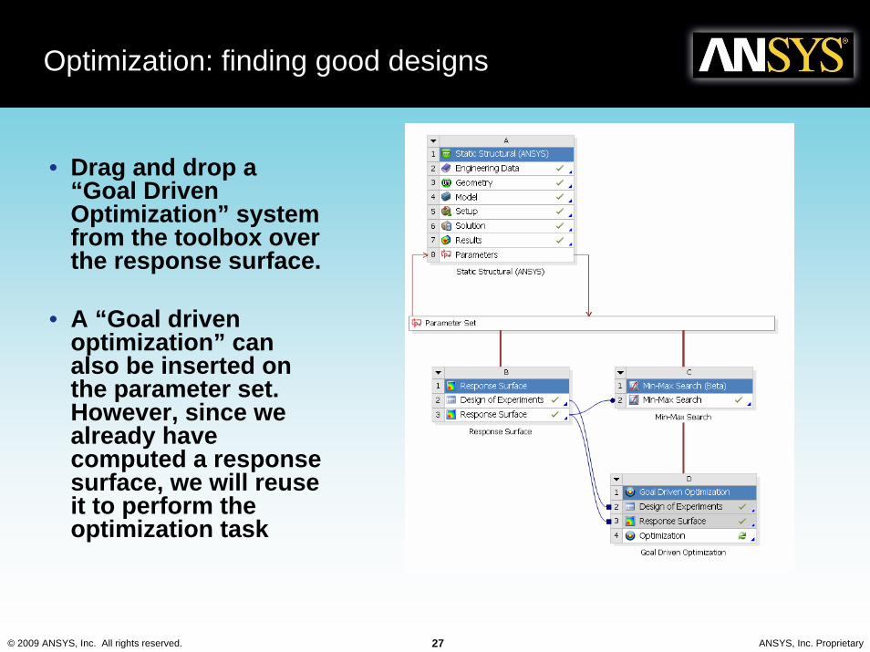
Optimization: finding good designs

• Drag and drop a “Goal Driven Optimization” system from the toolbox over the response surface.

• A “Goal driven optimization” can also be inserted on the parameter set. However, since we already have computed a response surface, we will reuse it to perform the optimization task


Setting up the goals

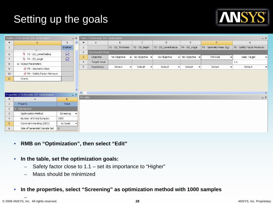
• RMB on “Optimization”, then select “Edit”

• In the table, set the optimization goals:– Safety factor close to 1.1 – set its importance to “Higher”– Mass should be minimized

• In the properties, select “Screening” as optimization method with 1000 samples–


Candidate designs

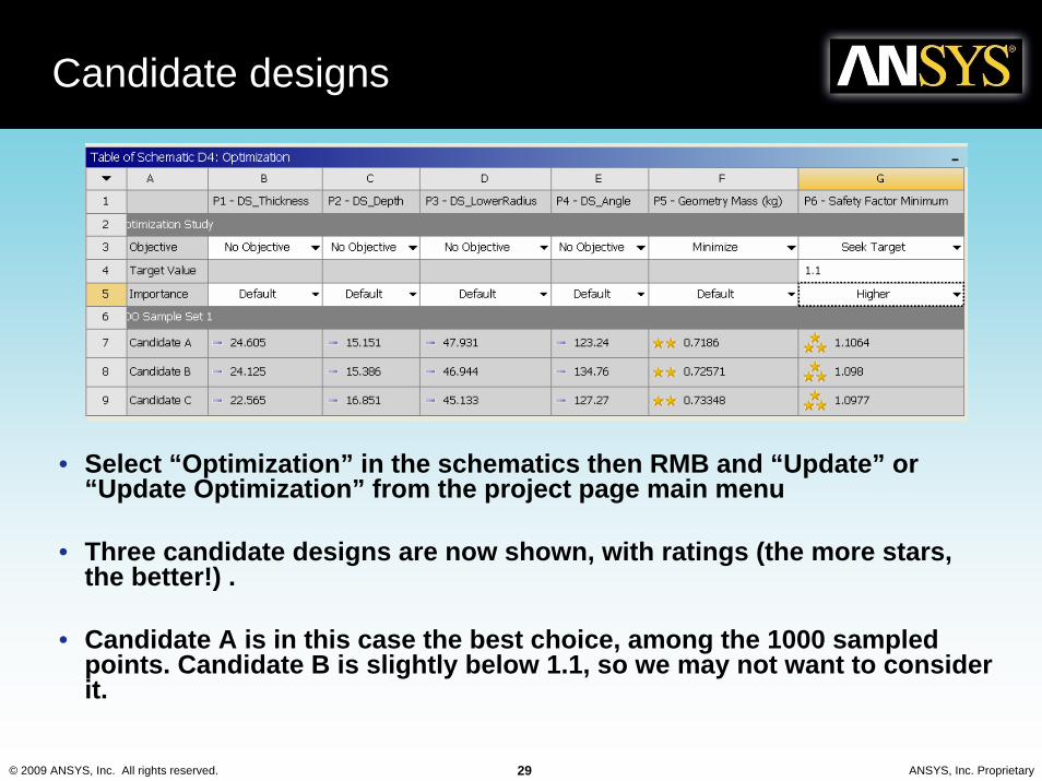
• Select “Optimization” in the schematics then RMB and “Update” or “Update Optimization” from the project page main menu

• Three candidate designs are now shown, with ratings (the more stars, the better!) .

• Candidate A is in this case the best choice, among the 1000 sampled points. Candidate B is slightly below 1.1, so we may not want to consider it.


TradeOff plots

• A tradeOff plot is a representation of the sample set we used for the goal driven optimization.

• It can be a 3D or 2D view of input or output parameters versus other parameters.

• Usually, a 2D plot is more readable than a 3D plot. In our particular case, since we are looking at 2 output parameters at the same time, the 2D plot is better suited.


TradeOff plots

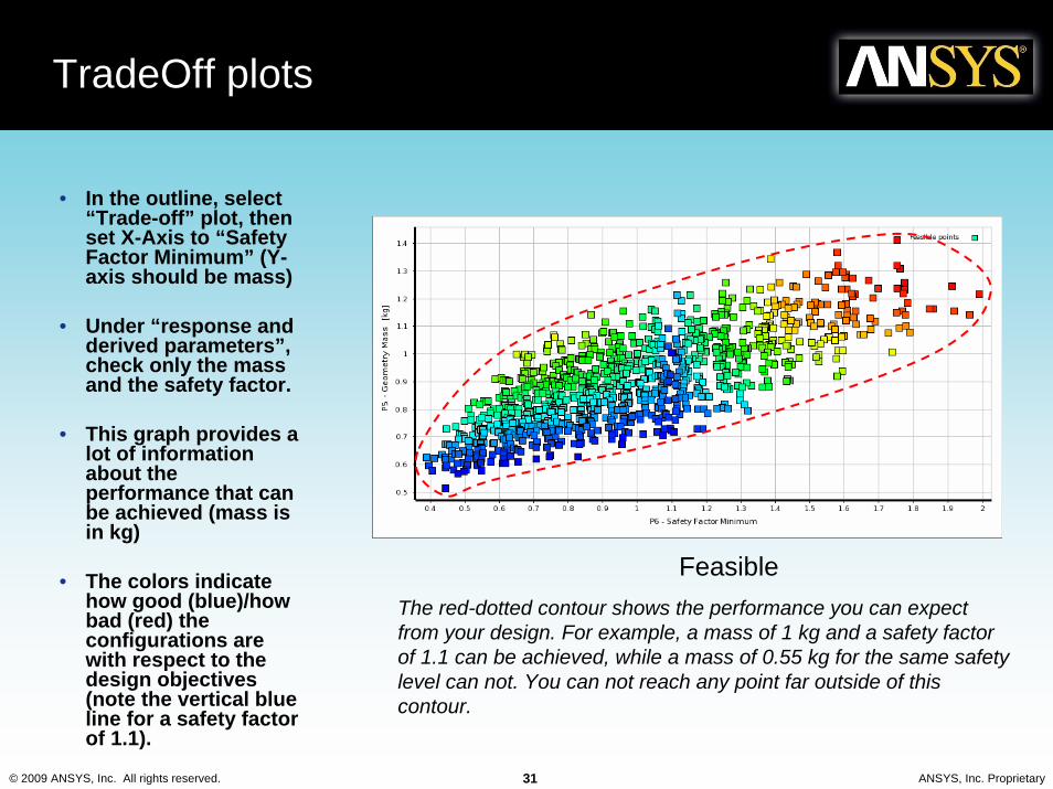
• In the outline, select “Trade-off” plot, then set X-Axis to “Safety Factor Minimum” (Y-axis should be mass)

• Under “response and derived parameters”, check only the mass and the safety factor.

• This graph provides a lot of information about the performance that can be achieved (mass is in kg)

• The colors indicate how good (blue)/how bad (red) the configurations are with respect to the design objectives (note the vertical blue line for a safety factor of 1.1).

The red-dotted contour shows the performance you can expect from your design. For example, a mass of 1 kg and a safety factor of 1.1 can be achieved, while a mass of 0.55 kg for the same safety level can not. You can not reach any point far outside of this contour.

Feasible


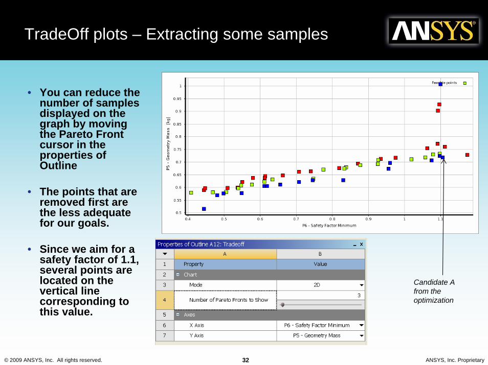
TradeOff plots – Extracting some samples

• You can reduce the number of samples displayed on the graph by moving the Pareto Front cursor in the properties of Outline

• The points that are removed first are the less adequate for our goals.

• Since we aim for a safety factor of 1.1, several points are located on the vertical line corresponding to this value.

Candidate A from the optimization


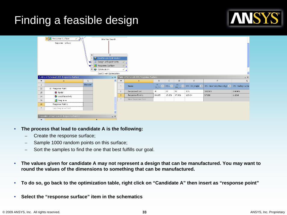
Finding a feasible design

• The process that lead to candidate A is the following:– Create the response surface;– Sample 1000 random points on this surface;– Sort the samples to find the one that best fulfills our goal.

• The values given for candidate A may not represent a design that can be manufactured. You may want to round the values of the dimensions to something that can be manufactured.

• To do so, go back to the optimization table, right click on “Candidate A” then insert as “response point”

• Select the “response surface” item in the schematics


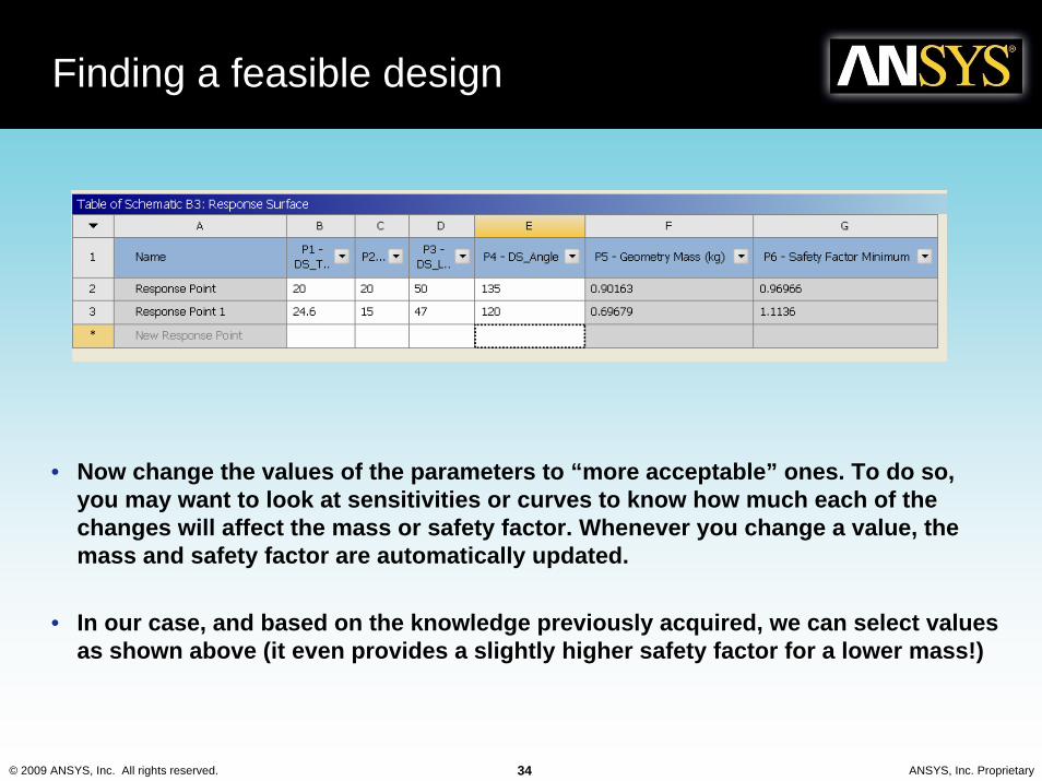
Finding a feasible design

• Now change the values of the parameters to “more acceptable” ones. To do so, you may want to look at sensitivities or curves to know how much each of the changes will affect the mass or safety factor. Whenever you change a value, the mass and safety factor are automatically updated.

• In our case, and based on the knowledge previously acquired, we can select values as shown above (it even provides a slightly higher safety factor for a lower mass!)


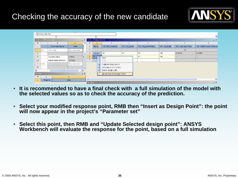
Checking the accuracy of the new candidate

• It is recommended to have a final check with a full simulation of the model with the selected values so as to check the accuracy of the prediction.

• Select your modified response point, RMB then “Insert as Design Point”: the point will now appear in the project’s “Parameter set”

• Select this point, then RMB and “Update Selected design point”: ANSYS Workbench will evaluate the response for the point, based on a full simulation


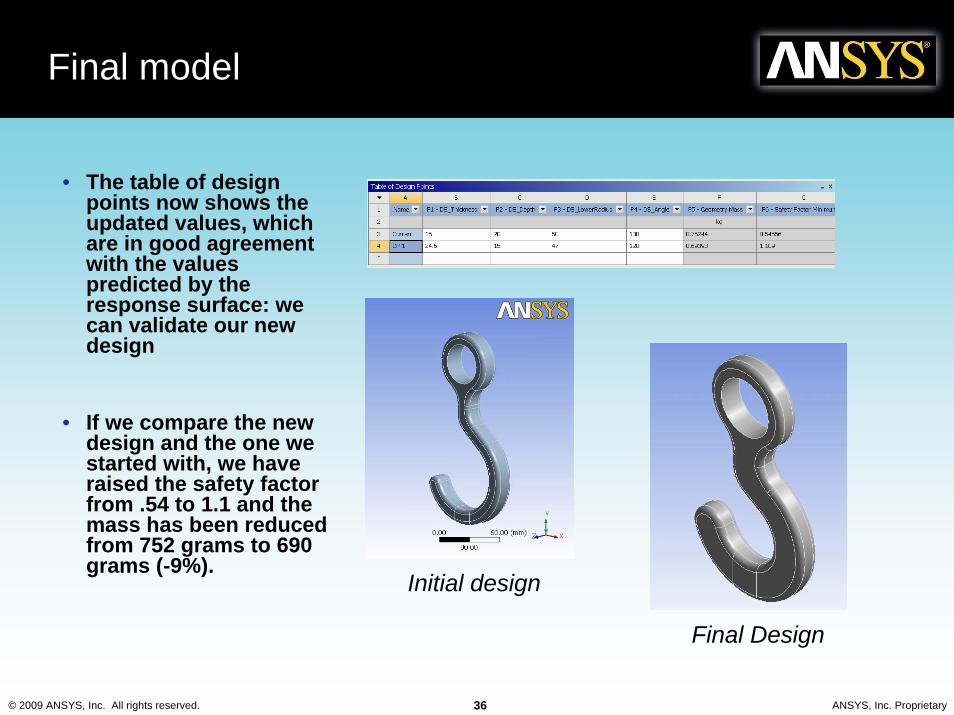
Final model

• The table of design points now shows the updated values, which are in good agreement with the values predicted by the response surface: we can validate our new design

• If we compare the new design and the one we started with, we have raised the safety factor from .54 to 1.1 and the mass has been reduced from 752 grams to 690 grams (-9%).

Initial design

Final Design


Good practice for the response surface analysis

• The response surface techniques used in DesignXplorer allow to work on a set of 5-10 input parameters at a time.

• Using more parameter will require much more simulations to provide a reasonable accuracy of the response surfaces.

• Always check your design candidates with a full simulation so as to remove the approximations due to the response surfaces.


Benefits of the deterministic analysis

• Benefits:– Using the deterministic analysis, we have been able to

investigate the performance of the design over continuous ranges of the input parameters, using a limited number of simulations.

– From the response surface, we are able to identify the key parameters really influencing the design.

– Also, we have been able to identify several candidates for the final design. Using engineering practice helps then to choose the final one.

– The deterministic approach helps identify the performance that can be reached with the actual design (TradeOff plots)

design exploration with ansys v12: the response surface method · design exploration with ansys...

Documents