July 2011

ECN-M--11-067

Design and Optimization of Tidal turbine AirfoilF. Grasso

29th AIAA Applied Aerodynamics Conference, 27-30 June 2011, Honolulu, HI, USA. AIAA 2011-3816

29th AIAA Applied Aerodynamics Conference Airfoil/wing/configuration aerodynamics

Design and Optimization of Tidal Turbine Airfoil

F. Grasso1

Energy Research Centre of the Netherlands (ECN), 1755 LE, Petten, The Netherlands

In order to increase the ratio of energy capture to the loading and thereby to reduce cost of energy, the use of specially tailored airfoils is needed. This work is focused on the design of an airfoil for marine application. Firstly, the requirements for this class of airfoils are illustrated and discussed with reference to the requirements for wind turbine airfoils. Then, the design approach is presented. This is a numerical optimization scheme in which a gradient based algorithm is used, coupled with RFOIL solver and a composite Bezier geometrical parameterization. A particularly sensitive point is the choice and implementation of constraints; in order to formalize in the most complete and effective way the design requirements, the effects of activating specific constraints are discussed. Particularly importance is given to the cavitation phenomenon. Finally, a numerical example regarding the design of a high efficiency, tidal turbine airfoil is illustrated and the results are compared with existing turbine airfoils.

Nomenclature α = angle of attack [deg] c = airfoil chord [m] Cd = airfoil drag coefficient [-] Cdmin = minimum airfoil drag coefficient [-] Cf = skin friction coefficient [-] Cl = airfoil lift coefficient [-] Clα = slope of the lift curve [deg-1] Clmax = maximum airfoil lift coefficient [-] Cmc/4 = airfoil moment coefficient referred to the quarter of chord [-] cp = pressure coefficient [-] F = objective function g = inequality constraints h = equality constraints H = boundary layer shape factor [-] L/D = aerodynamic efficiency [-] P0 = local pressure [Pa] Pv = vapour pressure [Pa] q = dynamic pressure [Pa] σc = cavitation parameter [-] X = design variables XL = lower bounds for the design variables XU = upper bounds for the design variables

1 Postdoctoral Aerodynamicist, Wind Energy Unit, Rotor and Wind Farm Aerodynamics Group, Westerduinweg 3; grasso@ecn.nl, Associate Fellow AIAA

I. Introduction UE to the intrinsic requirements in terms of design point, off-design capabilities and structural properties,

more and more, new airfoils families for wind turbines are developed [1-4]. However, apart from some development

done by Eppler [5], there are not specific studies in literature focused on airfoils for tidal turbines.

This work is focused on the design of a tidal turbine dedicated airfoil, by using numerical optimization. In the

next section, the requirements for this class of airfoils are presented, then the used design approach is explained.

Finally, the development of the new airfoil is described and the results are discussed.

II. Airfoils for Tidal Turbines

In the present section, the requirements for tidal turbine airfoils are illustrated, by using wind turbine airfoil

requirements as reference. A complete discussion for wind turbine airfoils can be found in [6].

A. Structural Requirements Airfoil characteristics include both aerodynamic and structural requirements. For the outer part of the blade, the

most important parameters, from the structural point of view, are the maximum airfoil thickness and the chord-wise

location of the maximum thickness. The thickness of the profile must be able to accommodate the structure

necessary for blade strength and stiffness. Depending of the class of the wind turbine, certain values for the

thickness along the blade can be expected and this fact introduces a first indication for the design problem. The

location of the maximum thickness along the chord is also important; when an airfoil is designed, also the other

airfoils along the blade should be considered to guarantee constructive compatibility. This means that, in order to

allow the spar passing through the blade, the chord-wise position of the thickness should be similar for the complete

blade.

B. Aerodynamic Requirements From the aerodynamic point of view the most important parameter for the tip region is the aerodynamic

efficiency (L/D). In order to obtain good turbine performance, the aerodynamic efficiency should be as high as

possible, but, at the same time, other considerations should be taken into account.

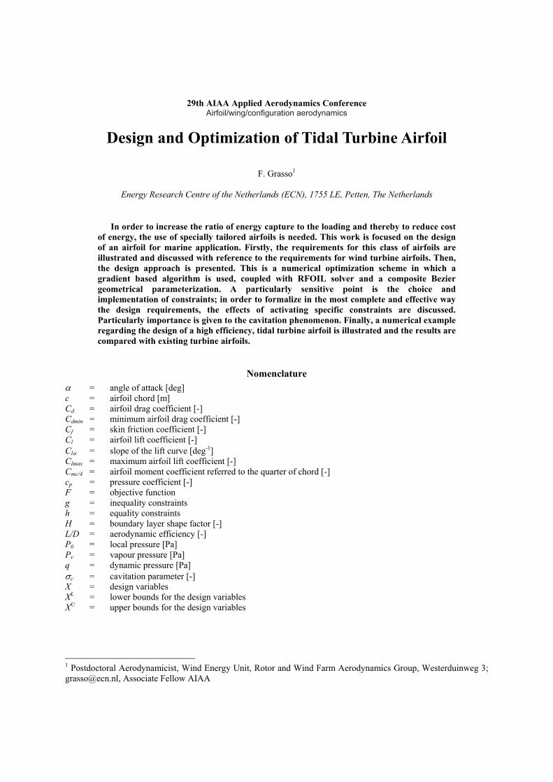
1. Cavitation The biggest difference between tidal and wind turbine airfoils is connected with the cavitation phenomenon.

Cavitation is the formation of vapor bubbles of a flowing liquid in a region where the pressure of the liquid falls

below its vapor pressure. Cavitation is usually divided into two classes of behavior: inertial (or transient) cavitation,

D

and non-inertial cavitation. Inertial cavitation is the process where a void or bubble in a liquid rapidly collapses,

producing a shock wave. Such cavitation often occurs in control valves, pumps, propellers, impellers, and in the

vascular tissues of plants. Non-inertial cavitation is the process in which a bubble in a fluid is forced to oscillate in

size or shape due to some form of energy input, such as an acoustic field. From the aerodynamic point of view, the

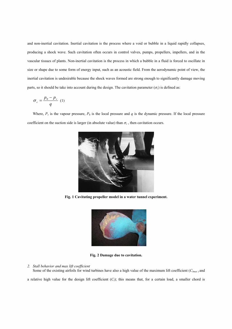
inertial cavitation is undesirable because the shock waves formed are strong enough to significantly damage moving

parts, so it should be take into account during the design. The cavitation parameter (σc) is defined as:

qpp v

c−

= 0σ (1)

Where, Pv is the vapour pressure, P0 is the local pressure and q is the dynamic pressure. If the local pressure

coefficient on the suction side is larger (in absolute value) than σc , then cavitation occurs.

Fig. 1 Cavitating propeller model in a water tunnel experiment.

Fig. 2 Damage due to cavitation.

2. Stall behavior and max lift coefficient

Some of the existing airfoils for wind turbines have also a high value of the maximum lift coefficient (Clmax ) and

a relative high value for the design lift coefficient (Cl); this means that, for a certain load, a smaller chord is

necessary. A lower chord in the outboard sections also reduces weight. For marine applications, the stall behavior is

important, more than the Clmax . So, the transition and the separation should move gradually when the angle of attack

increases. A high Cl value (and lower associated chord c) reduces the amplitude of load fluctuations resulting from

wind gusts and so fatigue loads. In water, the turbulence is lower; this means that problems connected with fatigue

have lower priority. In wind turbines, because of gusts, the local angle of attack for the single airfoil can suddenly

change and be in pre-stall or stall zone. So, it is important to have an angle of attack range between the design angle

of attack and the one for which, noticeable separation occurs on the airfoil. For tidal turbines, especially if the

turbine is a stall regulated turbine, it is convenient to reduce this margin to few degrees in order to use stall

mechanism to stop the turbine as soon the turbine overcomes the design condition.

3. Robustness to roughness Another important consideration is related with the sensitivity of the airfoil to the roughness. An airfoil with a

large laminar flow extension will be very efficient in “clean” conditions, but very bad in case of “dirty” conditions.

A large value for the leading edge can improve this aspect and, at the same time, it can help to avoid cavitation by

preventing from rapid expansions.

4. Blade torsion The moment coefficient (Cmc/4 ) should be taken into account because large values of moment coefficient will

give higher torsion moment on the blade. For tidal turbines however, the aspect ratio is lower than for wind turbines;

this means that the blade is more rigid regarding torsion deformation, so the blade torsion does not play a crucial

role in the design process.

III. Numerical Optimization Approach

In order to design airfoils, several methodologies can be used. A very popular approach is the inverse design

technique, proposed by Lighthill and widely developed by Eppler [5-7] and Drela [8, 9]. The basic principle of this

design method is that, the pressure coefficient on the airfoil surface is prescribed and the airfoil geometry is created;

by iteratively modifying the pressure distribution on the airfoil surface, the designer can generate the geometry of an

airfoil that satisfies the requirements. Despite its large use, there are several disadvantages associated with this

technique; the most evident is that it is very difficult to take into account at the same time multiple requirements,

especially when they concern different disciplines.

A valid alternative to solve this problem is the usage of multidisciplinary design optimization (MDO) approach.

In the most general sense, numerical optimization [10, 11] solves the nonlinear, constrained problem to find the set

of design variables, Xi, i=1, N, contained in vector X, that will:

Minimize )(XF (2) subject to:

0)( ≤Xg j Mj ,1= (3) 0)( =Xhk Lk ,1= (4) U

iiLi XXX ≤≤ Ni ,1= (5)

Equation 2 defines the objective function which depends on the values of the design variables, X. Equations 3

and 4 are inequality and equality constraints respectively (equality constraints can be written as inequality

constraints and included in equation 3), and equation 5 defines the region of search for the minimum. The bounds

defined for each degree of freedom by equation 5 are referred to side constraints.

C. Geometry Description One of the most important ingredients in numerical optimization is the choice of design variables and the

parameterization of our system in using these variables. In order to reduce the number of necessary parameters to

take into account to describe the airfoil’s shape, but without loss of information about the geometrical characteristics

of the airfoil, several mathematical formulations were proposed in literature [12]. In the present work, a composite

third order Bezier is used. Basically, the airfoil is divided in four parts and for each part, a third order Bezier curve is

used to describe the geometry. The advantage of this choice is the possibility to conjugate the properties of Bezier

functions in terms of regularity of the curve and easy usage, with a piecewise structure that allows also local

modifications to the geometry. The complete description can be found in [13]. a representative sketch is illustrated

in Fig. 3; the points between 1 and 4 define the first Bezier curve, the ones between 4 and 7 the second curve and so

on. In total, 13 control points are used to describe the airfoil geometry, that means 26 degrees of freedom. In

practice, however, the leading edge is fixed (control point 7), as well as the abscissa of the trailing edge (control

points 1 and 13); the abscissas of control points 6 and 8 are also fixed in order to maintain the curvature continuity at

the leading edge and the control points 4 and 10 are directly controlled by the algorithm to keep the curvature

continuity between two different Bezier curves.

12

345

6

7

8

9

10

11

12

13

Fig. 3 Geometry parameterization example.

D. Optimization Algorithm The choice of optimization algorithm is very important because the final results are usually dependent on the

specific algorithm in terms of accuracy and local minima sensitivity. Evolutionary algorithms are less sensitive to

local minima; however, they are time consuming and constraints have to be included as a penalty term to the

objective function. On the other hand, gradient based algorithms can lack in global optimality but allow multiple

constraints and are more robust, especially for problems in which a large number of constraints are prescribed. In

this investigation, an advanced sequential quadratic programming (SQP) gradient based algorithm [14] is

implemented and the gradients are approximated by finite differences.

E. Objective Function Evaluation Since the optimization process requires many evaluations of the objective function and the constraints before an

optimum design is obtained, the computational costs cannot be neglected, as well as the accuracy of the results.

Here, the RFOIL [15] numerical code is used. RFOIL is a modified version of XFOIL [16] featuring an improved

prediction around the maximum lift coefficient and capabilities of predicting the effect of rotation on airfoil

characteristics. Regarding the maximum lift in particular, numerical stability improvements were obtained by using

the Schlichting velocity profiles for the turbulent boundary layer, instead of Swafford’s. Furthermore, the shear lag

coefficient in Green’s lag entrainment equation of the turbulent boundary layer model was adjusted and deviation

from the equilibrium flow has been coupled to the shape factor of the boundary layer. The following figures

illustrate a comparison with experimental data [17] for the NACA-633418 airfoil. The Reynolds number is 6 million

and the transition is free.

00.20.40.60.8

11.21.41.61.8

0 2 4 6 8 10 12 14 16 18 20

alpha [deg]

Cl

experiments RFOIL XFOIL

Fig. 4 Lift curve for the NACA-633418 airfoil; comparison between XFOIL and RFOIL with experiments [17]. Reynolds number 6 million, free transition.

0

0.2

0.4

0.6

0.8

1

1.2

1.4

1.6

0.002 0.004 0.006 0.008 0.01 0.012 0.014 0.016

Cd

Cl

RFOIL experiments RFOIL+10% XFOIL

Fig. 5 Drag curve for the NACA-633418 airfoil; comparison between XFOIL and RFOIL with experiments [17]. Reynolds number 6 million, free transition.

It should be noted that the RFOIL prediction for the stall region is well described and very close to the

experimental data; in XFOIL results, only the deviation from the linear zone is described but not the stall. For the

drag curve, XFOIL and RFOIL are very close to each other for small values of Cl, but for high Cl, XFOIL is under

predicting. In [15], a additional drag of 10% is suggested to correct the RFOIL data; by adding this factor, a very

good agreement is found also for the drag coefficient. In order to have more realistic predictions, this 10% drag

penalty is added during the optimization process and for all the numerical analyses.

IV. Design of a New Airfoil for Tidal Turbines The design of a new airfoil is presented in this section. A stall regulated tidal turbine is chosen as reference; the

Reynolds number is 3 million and the airfoil is designed to maximize the aerodynamic efficiency at 7 degrees of

angle of attack. The same airfoil is used for all the blade.

The NACA0012 airfoil was used as baseline for the optimization. The purpose of this choice is to have a starting

point for the design process, as far as possible from potential local solutions and, in this way, have more confidence

on the optimality of the solution.

A. Geometrical Constraints A minimum value of 18% for the airfoil thickness is prescribed. As consequence, it should be noted that, because

of the 12% thickness, the baseline is even out of the feasible domain. The trailing edge thickness can change during

the design, allowing the algorithm to find the best value; however, a minimum value of 0.25% of the chord is

required in order to ensure airfoil’s feasibility from manufacturing point of view.

One of the problems outlined in the previous sections is the insensitivity for the roughness and the need to have a

smooth stall, with gradual transition and separation. By using the results of ESDU [18], a minimum value for the

ordinate at x/c equal to 0.0125c can be selected to ensure a trailing edge separation. From this parameter, a

minimum LE radius of 0.0155c can be assigned.

B. Aerodynamic Constraints To avoid possibility of abrupt stall and converge to a solution in which a Stratford style recompression is not

present (it can lead to a not gradual evolution in transition location), the design is performed by fixing transition at

0.01c on the suction side and 0.1c on the pressure side. However, to check the effect of the imposed transition on the

final geometry, the optimization is performed also in free transition condition.

As mentioned before, preventing from cavitation is the main issue for marine applications. In the present work,

the pressure coefficient (cp) distribution is calculated for each geometry and the expansion peak is compared to the

cavitation parameter. It is assumed a water temperature of 10° C, water depth equal to 1m and velocity of 10.5 m/s;

from these values, a value equal to 2 for the cavitation parameter is calculated.

C. Results Two airfoils have been designed: the G-hydra-A, obtained in free transition conditions and the G-hydra-B

obtained in fixed transition conditions. Fig. 6 shows the comparison between these new airfoils, the NACA 4418

airfoil and the DU96-w-180 airfoil.

NACA 4418 G-hydra-A G-hydra-B DU96-W-180

Fig. 6 G-hydra-A and G-hydra-B airfoils compared with NACA 4418 and DU96-W-180 geometries.

In Fig. 7 and Fig. 8, the aerodynamic characteristics are compared. Both airfoils improve the aerodynamic

efficiency and respect the set of constraints. The main difference between G-hydra-A and G-hydra-B geometries is

in the aft part of the airfoil. G-hydra-A airfoil is less cambered; because of this, the Cmc/4 (in absolute value) is

lower, as well as the lift curve. Looking at the stall, the characteristics of the G-hydra-B airfoil are quite good in

terms of quality of the stall and Clmax. Due to the concave shape on the suction side of the G-hydra-A airfoil, the lift

suddenly decreases as well as the efficiency, after the maximum is reached. Considering the G-hydra-B airfoil, there

is some margin between design asset and stall, but not so long as for the NACA 4418. For stall regulated turbines,

this can be an advantage because a little margin ensures that, from the design condition, the break mechanism (the

stall) starts to work before the turbine stay too long in off-design condition. Another good characteristic of the G-

hydra-B airfoil is that the linear part of the lift curve is quite extended compared to the reference geometries.

0

0.2

0.4

0.6

0.8

1

1.2

1.4

1.6

1.8

0 2 4 6 8 10 12 14 16 18 20

alpha [deg]

Cl

G-hydra-A NACA 4418 G-hydra-B DU96-W-180

Fig. 7 Lift coefficient curve; G-hydra-A and G-hydra-B airfoils compared to NACA 4418 and DU96-W-180 geometries. Reynolds number 3 million, free transition, RFOIL predictions.

0

20

40

60

80

100

120

140

160

180

0 2 4 6 8 10 12 14

alpha [deg]

L/D

G-hydra-A NACA 4418 G-hydra-B DU96-W-180

Fig. 8 Efficiency curve; G-hydra-A and G-hydra-B airfoils compared to NACA 4418 and DU96-W-180 geometries. Reynolds number 3 million, free transition, RFOIL predictions.

-2.50E+00

-2.00E+00

-1.50E+00

-1.00E+00

-5.00E-01

0.00E+00

5.00E-01

1.00E+00

1.50E+00

0 0.1 0.2 0.3 0.4 0.5 0.6 0.7 0.8 0.9 1

x/c

Cp5deg 6deg 7deg 8deg

Fig. 9 Pressure coefficient distribution.

-2.00E-03

3.00E-03

8.00E-03

1.30E-02

1.80E-02

0 0.1 0.2 0.3 0.4 0.5 0.6 0.7 0.8 0.9 1

x/c

Cf

8 deg 8.5 deg 9 deg 9.5 deg 10 deg 10.5 deg 11 deg 11.5 deg12 deg 12.5 deg 13 deg 13.5 deg 14 deg 14.5 deg 15 deg

Fig. 10 Cf

The same comparison have been performed by imposing the location of the transition at 5% of the chord, both

on the suction and the pressure sides.

0

0.2

0.4

0.6

0.8

1

1.2

1.4

1.6

1.8

0 2 4 6 8 10 12 14 16 18 20

alpha [deg]

Cl

G-hydra-A NACA 4418 G-hydra-B DU96-W-180

Fig. 11 Lift curve; G-hydra-A and G-hydra-B airfoils compared to NACA 4418 and DU96-W-180 geometries. Reynolds number 3 million, fixed transition, RFOIL predictions.

0

10

20

30

40

50

60

70

80

90

100

0 2 4 6 8 10 12 14

alpha [deg]

L/D

G-hydra-A NACA 4418 G-hydra-B DU96-W-180

Fig. 12 Efficiency curve; G-hydra-A and G-hydra-B airfoils compared to NACA 4418 and DU96-W-180 geometries. Reynolds number 3 million, fixed transition, RFOIL predictions.

Fig. 11 shows the comparison in terms of lift curve. Looking at the extent of the linear part, the value of

maximum lift coefficient and the quality of the stall, the lift curve of the G-hydra-B airfoil is almost unchanged in

fixed transition conditions. Because of the imposed transition, the aerodynamic efficiency decreases for all the

airfoils (Fig. 12), however the loss of the G-hydra-B airfoil are limited, especially if compared to the G-hydra-A

airfoil.

V. Conclusions

Two new airfoils for tidal turbines were designed. According to the RFOIL predictions, the results for one of

them (G-hydra-B) are promising when compared to the NACA 4418 and the DU96-W-180 airfoils. A good value

for the efficiency was achieved with separation limited only in the stall zone and without cavitation. Due to the

relatively large leading edge radius, the performances in off-design and rough conditions are also good, as well as

the stall that is quite smooth.

Despite these good results, wind tunnel tests are recommended to validate predictions. Especially for the stall

behaviour, the numerical predictions, and consequently the MDO process used in this work, need to be verified. In

absence of experimental data, the stall characteristics have been compared with the above mentioned work from

ESDU; according to these data, the stall for the G-hydra-B airfoil is expected to be due to trailing edge separation.

Acknowledgments The author would like to thank Dr. H. Snel for the precious help and suggestions during this work.

References

[1]. Tangler, J.L., Somers, D.M., “NREL Airfoil Families for HAWT’s”. Proc. WINDPOWER’95, Washington D.C., 1995; pp.

117–123.

[2]. Björk, A., “Coordinates and Calculations for the FFA-W1-xxx, FFA-W2-xxx and FFA-W3-.xxx Series of Airfoils for

Horizontal Axis Wind Turbines”. FFA TN 1990-15, Stockholm, Sweden 1990.

[3]. Timmer, W.,A., van Rooij, R.P.J.O.M., “Summary of the Delft University Wind Turbine Dedicated Airfoils”. AIAA-2003-

0352.

[4]. Fuglsang, P., Bak, C., “Design and Verification of the new Risø-A1 Airfoil Family for Wind Turbines”. AIAA-2001-0028.

[5]. Eppler, R., “Airfoil Design and Data”, Springer Verlag, 1990.

[6]. Grasso, F., “Usage of Numerical Optimization in Wind Turbine Airfoil Design”, 28th Applied Aerodynamics Conference,

AIAA, Chicago, IL, USA, 28June-1July, 2010, AIAA 2010-4404. Also accepted for Journal of Aircraft,

[7]. Eppler, R., Somers, D.M., “A Computer Program for the Design and Analysis of Low-Speed Airfoils”, NASA-TM-80210,

1980.

[8]. Drela, M., “XFOIL: An Analysis and Design System for Low Reynolds Number Airfoils, Conference on Low Reynolds

Number Airfoil Aerodynamics”, University of Notre Dame, June 1989.

[9]. Drela, M., Giles, M.B., “Viscous-Inviscid Analysis of Transonic and Low Reynolds Number Airfoils”, AIAA Journal, Vol.

25, October 1987, pp. 1347-1355.

[10]. Fletcher, R., “Practical Methods of Optimization”, Wiley, 1987.

[11]. Pedregal, P., “Introduction to Optimization”, Springer, 2004, ISBN 0-387-40398-1.

[12]. Samareh, J., A., “Survey of Shape Parameterization Techniques for High-Fidelity Multidisciplinary Shape Optimization”,

AIAA Journal, Vol. 39, No. 5, May 2001, pp. 877-884.

[13]. Grasso, F., “Multi-Objective Numerical Optimization Applied to Aircraft Design”, Ph.D. Thesis, Dip. Ingegneria

Aerospaziale, Università di Napoli Federico II, Napoli, Italy, December 2008.

[14]. Schittkowski, K., “NLPQLP: A new Fortran implementation of a sequential quadratic programming algorithm - user’s

guide, version 1.6”, Report, Department of Mathematics, University of Bayreuth, 2001.

[15]. van Rooij, R.P.J.O.M., “Modification of the boundary layer calculation in RFOIL for improved airfoil stall prediction”,

Report IW-96087R TU-Delft, the Netherlands, September 1996.

[16]. Drela, M., “XFOIL 6.94 User Guide”, MIT Aero & Astro, Dec 2001.

[17]. Abbott, I., Von Doenhoff, A., “Theory of Wing Sections”, Dover Publications, Inc., Dover edition, 1958.

[18]. ESDU, “The low-speed stalling characteristics of aerodynamically smooth airfoils”, ESDU 66034, UK, October 1966.