design and optimization of energy systems prof. c. balaji...
TRANSCRIPT
Design and Optimization of Energy Systems
Prof. C. Balaji
Department of Mechanical Engineering
Indian Institute of Technology, Madras
Lecture - 06
Successive Substitution Method
(Refer Slide Time: 00:22)
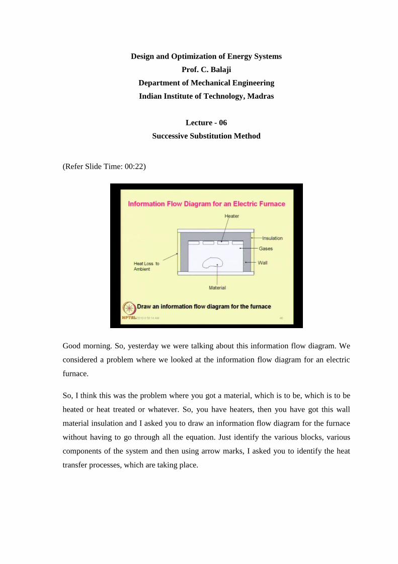
Good morning. So, yesterday we were talking about this information flow diagram. We
considered a problem where we looked at the information flow diagram for an electric
furnace.
So, I think this was the problem where you got a material, which is to be, which is to be
heated or heat treated or whatever. So, you have heaters, then you have got this wall
material insulation and I asked you to draw an information flow diagram for the furnace
without having to go through all the equation. Just identify the various blocks, various
components of the system and then using arrow marks, I asked you to identify the heat
transfer processes, which are taking place.
(Refer Slide Time: 00:52)
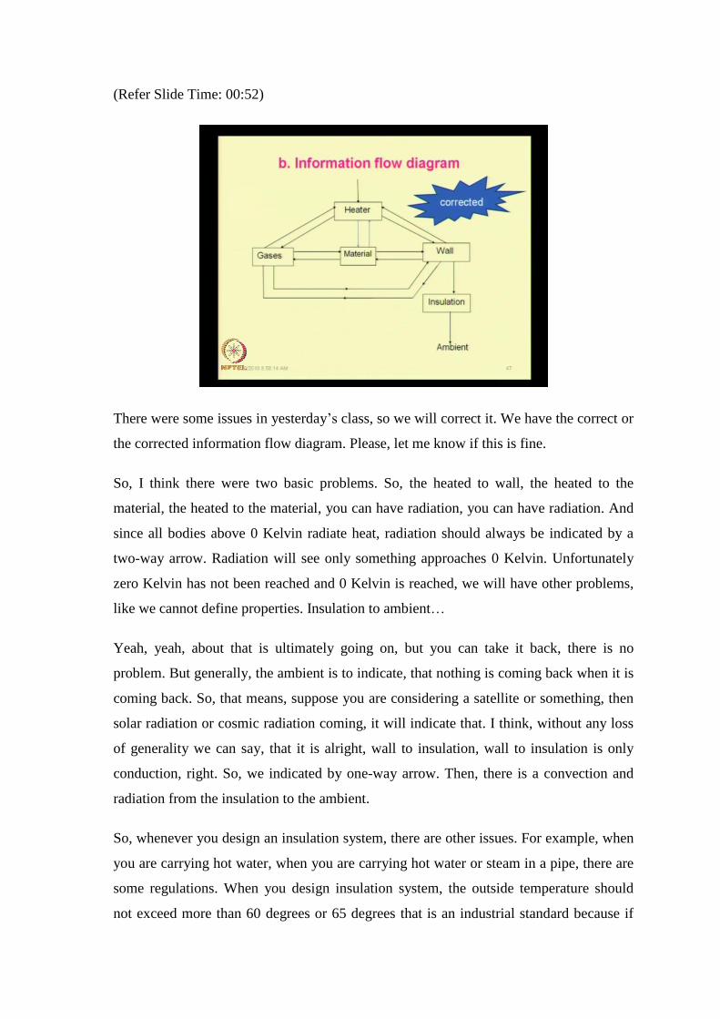
There were some issues in yesterday’s class, so we will correct it. We have the correct or
the corrected information flow diagram. Please, let me know if this is fine.
So, I think there were two basic problems. So, the heated to wall, the heated to the
material, the heated to the material, you can have radiation, you can have radiation. And
since all bodies above 0 Kelvin radiate heat, radiation should always be indicated by a
two-way arrow. Radiation will see only something approaches 0 Kelvin. Unfortunately
zero Kelvin has not been reached and 0 Kelvin is reached, we will have other problems,
like we cannot define properties. Insulation to ambient…
Yeah, yeah, about that is ultimately going on, but you can take it back, there is no
problem. But generally, the ambient is to indicate, that nothing is coming back when it is
coming back. So, that means, suppose you are considering a satellite or something, then
solar radiation or cosmic radiation coming, it will indicate that. I think, without any loss
of generality we can say, that it is alright, wall to insulation, wall to insulation is only
conduction, right. So, we indicated by one-way arrow. Then, there is a convection and
radiation from the insulation to the ambient.
So, whenever you design an insulation system, there are other issues. For example, when
you are carrying hot water, when you are carrying hot water or steam in a pipe, there are
some regulations. When you design insulation system, the outside temperature should
not exceed more than 60 degrees or 65 degrees that is an industrial standard because if
somebody goes and touches, then we will get scalded or burnt and so on. So, the, so you
fix the outside temperature 65, then you turn around and calculate what will be the, what
will be the insulation thickness and if you decide on a particular type of material and
then there is an optimization, which is possible for various values of thickness of the
material, for various types of material, you can work out the insulation. Some materials
are banned, for example, asbestos is carcinogenic and so on. So, there are lots of issues,
which will be outside engineering when you have finally decided on what is the
appropriate system you want to use. Are you getting the point?
Now, we will proceed with our successive substitution, but I will first dictate the
problem, you take it down and then, I will show the same problem on the PowerPoint.
You start working and I will also work it out on the board, so that we are able to
convergent on a particular solution.
Problem number 6, system simulation. Consider an electrically heated wire of emissivity
0.6, consider, consider an electrically heated wire of emissivity 0.6, full stop. Under
steady state conditions, consider an electrically heated wire of emissivity 0.6, under
steady state conditions the energy input to the wire, under steady state conditions the
energy input to the wire is 1000 watts per meter square, under steady state conditions the
energy input to the wire is 1000 watts per meter square of surface area of the wire. The
energy input to the wire is 1000 watts per meter square of surface area of the wire and
the heat transfer coefficient, and the heat transfer coefficient to the ambient is, the heat
transfer to the ambient is 10 watts per meter square per Kelvin, 10 watts per meter square
per Kelvin. The ambient temperature is 300 Kelvin; the ambient temperature is 300
Kelvin.
1, what is the energy equation governing the steady state temperature of the wire? 1,
what is the energy equation governing the steady state temperature of the wire? What is
the energy equation governing the steady state temperature of the wire? B, B or 2, using
the method of successive substitution, using the method of successive substitution,
determine, using the method of successive substitution, determine the steady state
temperature of the wire, using the method of successive substitution determine the steady
state temperature of the wire.
(Refer Slide Time: 06:02)
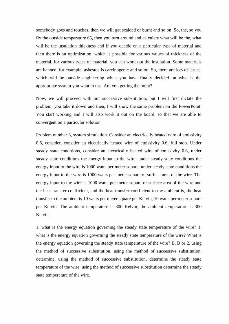
So, people who have not been able to be follow this or people who came late, whatever I
dictated now has been put up on PowerPoint. For the sake of completeness, I added one
more part to decide on an appropriate stopping criterion. To the critical data, it is losing
heat by both, convection and radiation. Surface emissivity is given, h is given, surface
area is not required because I have given power density as watts per meter square.
So, first draw a sketch, there is no need to draw an information flow diagram. If you
want you can, it is only a single component, it is not very difficult. You can go ahead and
draw the information flow diagram or a sketch of the system. Indicate all the heat
transfer processes, which are taking place. Write down the governing equation, and then
start solving.
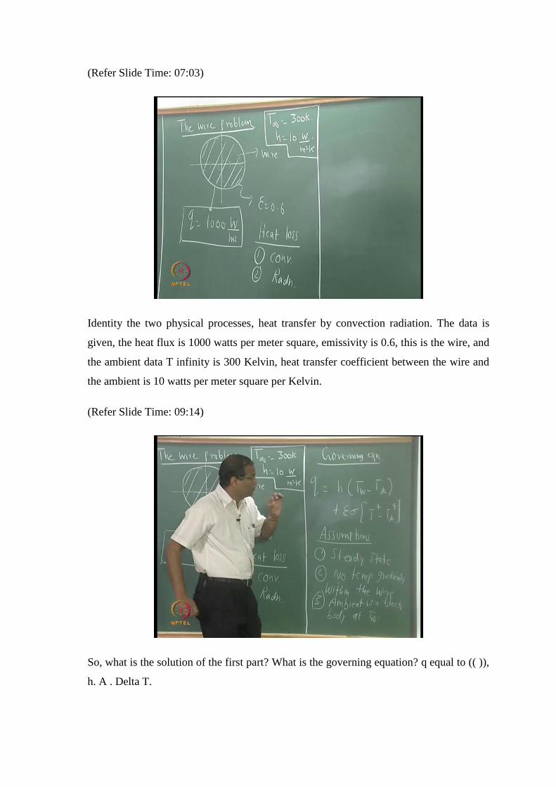
(Refer Slide Time: 07:03)
Identity the two physical processes, heat transfer by convection radiation. The data is
given, the heat flux is 1000 watts per meter square, emissivity is 0.6, this is the wire, and
the ambient data T infinity is 300 Kelvin, heat transfer coefficient between the wire and
the ambient is 10 watts per meter square per Kelvin.
(Refer Slide Time: 09:14)
So, what is the solution of the first part? What is the governing equation? q equal to (( )),
h. A . Delta T.
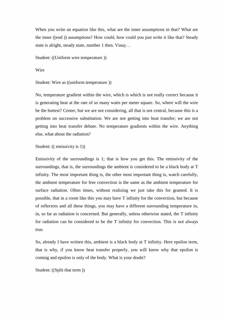
When you write an equation like this, what are the inner assumptions in that? What are
the inner ((end )) assumptions? How could, how could you just write it like that? Steady
state is alright, steady state, number 1 then. Vinay…
Student: ((Uniform wire temperature ))
Wire
Student: Wire as ((uniform temperature ))
No, temperature gradient within the wire, which is which is not really correct because it
is generating heat at the rate of so many watts per meter square. So, where will the wire
be the hottest? Center, but we are not considering, all that is not central, because this is a
problem on successive substitution. We are not getting into heat transfer; we are not
getting into heat transfer debate. No temperature gradients within the wire. Anything
else, what about the radiation?
Student: (( emissivity is 1))
Emissivity of the surroundings is 1; that is how you get this. The emissivity of the
surroundings, that is, the surroundings the ambient is considered to be a black body at T
infinity. The most important thing is, the other most important thing is, watch carefully,
the ambient temperature for free convection is the same as the ambient temperature for
surface radiation. Often times, without realizing we just take this for granted. It is
possible, that in a room like this you may have T infinity for the convection, but because
of reflectors and all these things, you may have a different surrounding temperature in,
in, so far as radiation is concerned. But generally, unless otherwise stated, the T infinity
for radiation can be considered to be the T infinity for convection. This is not always
true.
So, already I have written this, ambient is a black body at T infinity. Here epsilon term,
that is why, if you know heat transfer properly, you will know why that epsilon is
coming and epsilon is only of the body. What is your doubt?
Student: ((Split that term ))
There is no epsilon, that epsilon is only for the, epsilon is only for the, for the body.
People who take in conduction and radiation, those I spend an hour, half an hour as so, I,
explaining how this formula, why this formula is the most abused formula in heat
transfer. Simply, people say radiation epsilon sigma T to the power 4 minus, I derived
this from first principle using two body enclosure and I proved in my class, in my
conduction radiation class, that this, so many assumptions are there. So, I do not have the
time now, we are also live on this thing, but if you want I can show it to you at end of the
class. So, you have to use a two body enclosure, you can just show by simple physics, so
that epsilon is equal to 1.
His doubt is, since epsilon is outside the bracket, he is, he is having a problem whether
there is an epsilon of the surroundings also. There is no epsilon in so far as, surroundings
is concerned. See, this problem can be solved either using the network theory or using
what is a radiastic radiation method. I teach only the radiastic radiation method using the
radiastic radiation method in 15 minutes. You can show this is the formula you get for,
for a small, small body in a large enclosure, alright. Now, go ahead and knowing fully
well or knowing fully well, what the assumptions are, go ahead and start doing the
iteration.
Serial number T i instead of T w, you can just take it as T. T i, T i plus 1, T i plus 1
minus T i whole square, that is error criterion decided, decided on an appropriate
stopping criterion. And I can tell you, that two types of information flow diagram are
possible and in one of the information flow diagram the solution will diverge. Some of
you will, will tell me, Sir, this will, it is not converging. Then, we will have to turn
around and use the other information flow diagram. Please start.
So, if you recall we are still trying to study system simulation. I told you, that I will teach
you system simulation by looking at two or three techniques to solve the system of non-
linear algebraic equations. We started with a method of successive substitution.
Yesterday’s class, we started with a simple mathematical problem x equal to 2 sine x.
Now, we proceeded to a problem in thermal systems or most, more specifically a
problem in heat transfer, which has got one component. After you finish, as soon as you
finish this we will go to a thermal system, I mean, a fluid thermal system with two
components, so, so that will reinforce the, once that will reinforce your understanding of
this method of successive substitution.
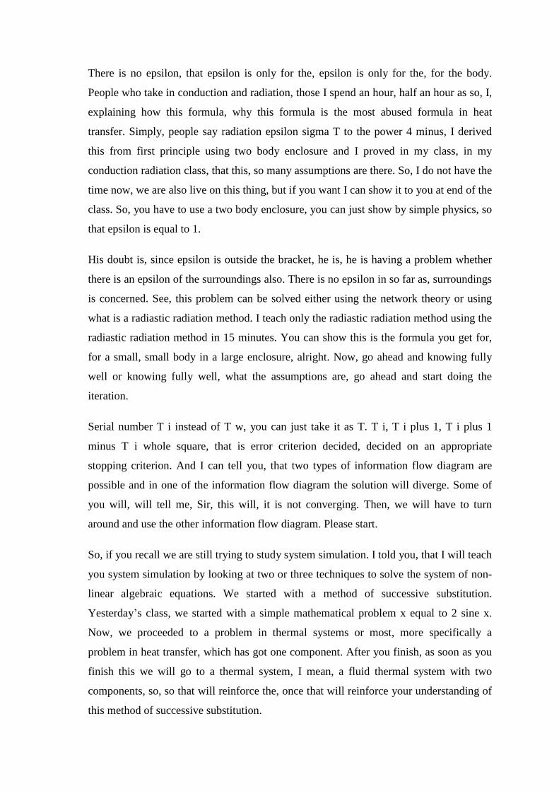
Now, what do you want to?
(Refer Slide Time: 15:58)
So, what you want the algorithm to be? I just…
Is it ok? Or…
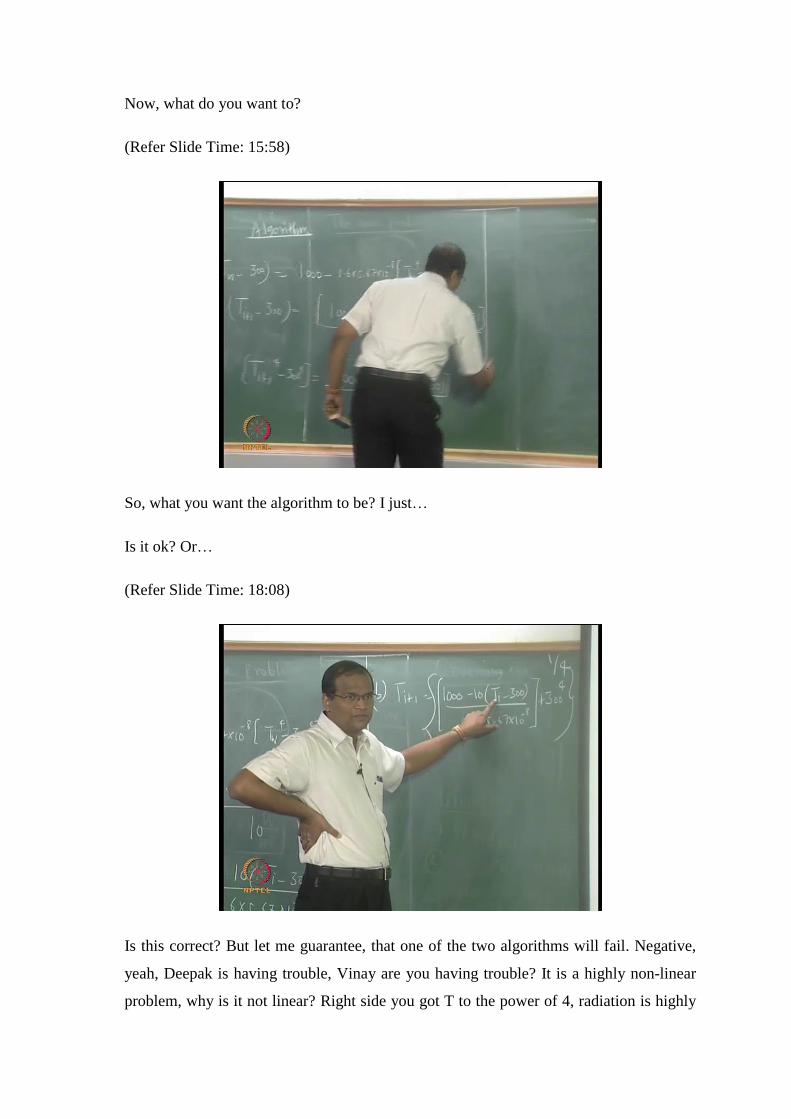
(Refer Slide Time: 18:08)
Is this correct? But let me guarantee, that one of the two algorithms will fail. Negative,
yeah, Deepak is having trouble, Vinay are you having trouble? It is a highly non-linear
problem, why is it not linear? Right side you got T to the power of 4, radiation is highly
non-linear. I do not think, you have solved problems like this in heat transfer course are,
it is very unstable. So, one of the two algorithms will cup, we will not investigate why it
is so, why one of the two algorithms is not working and so on. But suffice it would to
say, that because of T to the power of 4, one of the two algorithms will not work. So,
because the errors will propagate, but you know, that it is a physical problem.
A wire is cooling, it has got emissivity, there is natural convection, there convection and
radiation, so it has to attain a physical temperature. If at all you get negative temperature,
it is not because of Physics, 1000 watts per meter square is a reasonable flux, emissivity
is reasonable, ambient temperature is reasonable, h is reasonable. Therefore, you should
get the reasonable temperature as the answer. If you get an unphysical solution, that
means, a problem is not with the Physics, but the problem is with your algorithm. So, we
can say, that this is a, this b. Deepak which one fails?
First one fail, second one fails, second one fail. So, let me, so people who already started,
actually I want it to try both, you will realize that. Now, why you are smiling? It is not a
painful problem. So, you, you can very well realize, that even one component is not so
simple as you thought. Suppose, I have two component system, if it is non-linear, it will
give lot of trouble. Two component system if you give you in the exam quiz, whatever, it
will take half an hour, 40 minutes.
Suppose, I give many terms in the equation, and it is going to take a lot more time. Of
course, it is eminently, it is, it is eminently doable by using a script file Matlab or writing
your own code and all that, but, but for the purpose of exam you have to use calculator
and we have to use calculator and pen and proceed, alright. Yeah…
Student: (( 366))
Is it?
Student: 366
366
366.4 or something. Let us solve this. Vikram got it? Which one, which algorithm you
use? First one, how many of you use a second one? What it, what happen? What is the
problem there?
Student: (( T is increasing and thousand minus thing is changing like this))
That is the problem. So, because of this, this, if the T increases, what is a maximum
possible for this? The moment it exceeds 400 it is gone. The moment it exceeds 400,
then (( this)) algorithm is in struggle because it is over shooting. I mean, if you, if you
actually take the slope, another things, you can investigate mathematically, but that is not
central to our our discussion here.
So, if you solve this problem using the method of successive substitution, if you
encounter a difficulty, if you get an answer, which is negative or is diverging, you are not
able to proceed further. You should not say, that this problem has no solution because
from what, from the data given to you, given to you, it is so clear, that there is a solution,
which is the problem. Immediately, you should think of the other information flow
diagram.
What, what, what is the information flow diagram I am talking about here? Basically,
whether q convection is equal to total q minus q radiation or q radiation is equal to total q
minus q convection, these are the two information flow diagram. So, here I am saying, q
convection is q total minus q radiation. Here, I am saying, that q radiation is q total
minus q convection. It so happens, that one of the two is not working. So, when one of
the information flow diagrams is not working, go to the other information flow diagram.
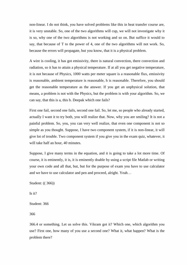
(Refer Slide Time: 23:10)
What is 376.5? How many of you started with 350 and why did you take 350? The
reasonable, 350 appear to be reasonable. Why are you… It cannot be at 1000 degree,
1000 Kelvin or something. 350 appear to be reasonable. So, so we should put Kelvin.
What about this unit? 350, you get 376.5. What you get? How many of you are troubled?
Why are the, why is the class so silent? Venugopal, you got it?
Student: ((ok ))
Vaibhav got it? Vikarm has got it, you? So, 376.5, what is it now, is too much, what is
this? 700. I worked it out last night, so I have the numbers. 359.1, I am allowed not to
write this now because I am the teacher, but you have to. So, you just, because I know it
is not converging, 359, 4. So, do not feel lazy, you have to fill up all this. Number 6 was
368.5, 364.8, 14. Did somebody proceed beyond the 14th iteration? 366.4, it is like 90,
93 degree Celsius, alright. ((Ok )), for those people whose information flow diagram
corresponding to algorithm 2 or algorithm b cup, you please go back and substitute this
366.4, and see whether now it works. Exactly at that point it will work, just check, it
should work, right. Any other point?
It is very unstable algorithm that is the problem; it is very unstable. That is basically,
because if you take f of x, sorry, f of t equal to q minus total q minus q convection minus
q radiation, if you take dou of f of x or d of f of x by d 2, that is, if you plot, that fellow is
a very strong function of temperature because it is 3 t cube and all that. So, he is not
behaving properly, he is misbehaving, that is why you are not able to. So, if you want to
investigate easily, you can go to Matlab and investigate why it happens.
You just take the first derivative, it is highly oscillatory. So, you have to, you have to
always guess in the right region and it will not allow because of t to the power of 4. Once
you start with, unless you are, unless you start a 366.4 or 366 itself, it will swing to the
right side or the left side. And if you are so, if you are so sure, that you have to start with
366.4, then Swamiji (( you can say)), this is the answer I mean. So, you do not require
method of successive substitution because you know everything.
So, that is why, yeah, now 366.4, did you substitute in to the other one? Please, please
check that. So, why x equal to 2 sine x? It was the very simple problem and I wrote, we
wrote the algorithm yesterday and solved, there are no issues; note, there are issues of
divergence already.

So, all the information flow diagrams are not the same, some are more equal than the
others. It is possible for you to get a solution with one information flow diagram while it
is perfectly possible for you not to get a solution, the other information flow (( diagram)).
In the exam if you give a highly non-linear problem, you start with an information flow
diagram and you do not get the answer, you are unlucky. Then, you have to switch over
to the a priori, I do not know whether to, otherwise you have to take the derivative and
all that. The time taken for that, you might as well start with this information flow
diagram, get (( up)) and proceed to the point at which the solution diverges and turn
around and say, that this this information flow diagram does not work, so I will have to
go back to the other information flow diagram. Is it ok?
(Refer Slide Time: 29:20)
So the solution is, 90…
Does it work? Well said, so if you are started, probably 366 point, 367 or 366, may be it
work, may be it would have work. If you start with 350 or if you start with 400, it may,
anyway, you cannot start beyond 400 because it becomes negative. So, these are the
issues associated with this, fine.
Now, we will go to a problem where we take a real fluid thermal system, namely the fan,
and namely a fan and duct system. So, this is going to take about 40 minutes, you are not
going to able to solve this in today’s class completely, but nevertheless we will start.

(Refer Slide Time: 30:47)
So, let us go to system simulation. Let us talk about some practical situation. You are
designing a ducting system for a, you are designing a ducting system for an air
conditioner on auditorium for the ICSR building. You are deciding about the fan
capacity. I am not talking about the chiller capacity, and how many tons of refrigeration
you want and all, you want to send chilled air. You have to decide on the ducting, fan
and ducting system, correct.
Now, it is possible for you to calculate the total length, total length of the duct, how may
bends are there. Then, flv square by 2gd, and then k flv square by 2gd and all, you can
add all these and put everything as a functional velocity or discharge and get a formula
for calculating a total pressure drop. If you have the total pressure drop multiplied by the
discharge it is, and if you know the fan efficiency, if you know the approximate
efficiency, you will, you will have an idea of how much of power is required. But for
overcoming a particular head, for overcoming a particular head, you also, you also will
know what is the discharge corresponding to that head from the manufacturers operating
characteristics or these are called fan curves, you must have studied in turbo-machines.
Now, if you eventually have to decide have to design the fan and ducting system, the fan
characteristics of the manufacture have to match the load characteristics of a particular
design. When these two intersected at particular point, this is called the operating point
that means, you have done the system simulation to determine the operating point.
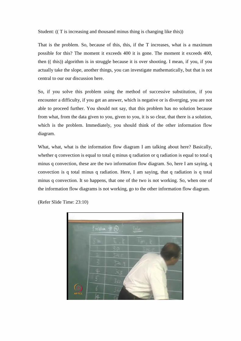
(Refer Slide Time: 32:55)
So, graphically, so if you consider, you, is it like this correct. So, this is what is, what is
this? Fan curve, what about that curve? This could be meters or it could be, whatever,
this will be meter cubes per second. So, this is the operating point. Using system
simulation, we want to calculate this operating point. This can be easily calculated
because this is based on a formula, right. If you know the friction factor, if you know the
friction factor and all this, you can calculate. How do we get this?
So, this you have to get from the manufactures catalogue or whatever. How, how will he
have got this? So, basically you have to do experiments. You will, you will first do
experiment with no discharge, 0 discharge, then will slowly increase the discharge and
you will find out the head and you will find, do an experiment connecting this. And so,
therefore, you may get some points like this.
But if you want to do simulation, you just have point; it is no good for you because you
want a curve, right. So, you will convert all this points into an approximate, into a, into a
best fitting curve using principles of regression. That is why I said, regression is very
important for system simulation, but if start teaching regression upfront before teaching
system simulation, you will see, you will think what this course is all about mathematics
and we thought we will learn design and optimization is only regression.
So, last year I first start regression and then went system simulation. This time I am
swap. I will teach you system simulation, so that you get a feel, that regression is very,
very important to get this. You are getting the point? Once you have these two curves,
then you determine the operating point, then you have to determine, you have to
determine the sensitivity of your operating point. For example, it is possible, that with
time or something there could be multiple fan curve can go up and down. This can also
go on up and down depending upon the age and other things and friction factor may
increase or the efficiency of the pump may decrease and so on. So, you will have to
study the sensitivity of the performance of the equipment of the system with respect to
the change the design operating conditions, alright.
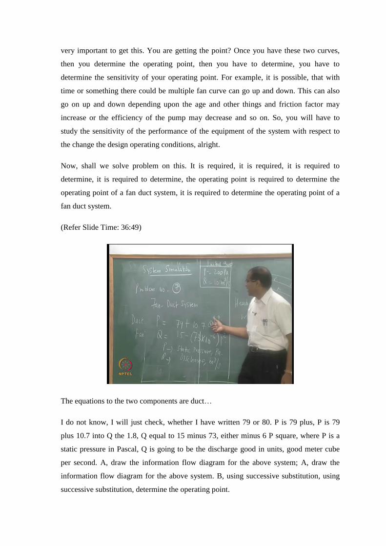
Now, shall we solve problem on this. It is required, it is required, it is required to
determine, it is required to determine, the operating point is required to determine the
operating point of a fan duct system, it is required to determine the operating point of a
fan duct system.
(Refer Slide Time: 36:49)
The equations to the two components are duct…
I do not know, I will just check, whether I have written 79 or 80. P is 79 plus, P is 79
plus 10.7 into Q the 1.8, Q equal to 15 minus 73, either minus 6 P square, where P is a
static pressure in Pascal, Q is going to be the discharge good in units, good meter cube
per second. A, draw the information flow diagram for the above system; A, draw the
information flow diagram for the above system. B, using successive substitution, using
successive substitution, determine the operating point.
An important thing here is the initial guess. Of course, using common sense you can
arrive at an initial guess, but since it is a class room environment, I will give you the
initial guess. You can either take P is 200 Pascal or Q is 10 meter cube per second.
First draw the information flow diagram, draw two components – fan and duct. Draw
two rectangular boxes, something will go in, something will go out, then complete it, this
is a, this is a sequential arrangement because output of the fan becomes input to the duct,
output of the duct becomes input to the fan.
Two types of information flow diagram are possible, watch out two types of information
flow diagrams are possible, please look at the board. You can you can use this equation
to determine P, if you know Q. There is, but there is no hard and fast rule about this. I
can say, that Q to the power of 1.8 is P minus 79 divided by 10 point7 or rather, Q is
equal to P minus 79 divided by 10.7 whole to the power of 1 by 1.8. So, I could try
convert this. Do not think that this is on the left hand side, this is on the right hand side, I
cannot do anything about it. This equation can be used, to cut a long story short, this
equation can be used to calculate P given Q or vice versa. By the same token, this
equation need not be necessarily useful to calculate Q, you can also calculate P from Q
depending on this.
If you want to calculate P from this equation and Q from this equation, that is shown
information flow diagram. If you want to swap, that is another information flow diagram.
And since you have got non-linear powers, one is P square, one is Q to the power of 8,
one of the two information flow diagrams will, will not, one of the information flow
diagram will not, will not work. So, let us see who is unfortunate and, and in tomorrow’s
class in the, I mean in next Thursday, Monday is holiday, Thursday’s class. We will
solve this problem and investigate now, why one of the information flow diagram, why
is it not working. So, please draw the information flow diagram first, and now any
guesses on how you got this Q to the power of 1.8.
Student: (( Regression))
Correct, regression physics, what is the physics with this 1.8? 4 flv square diameter is
fix, you know, I usually in this, I am fixing that dimensions, it could be a diameter of
pipe, it got be the, it could be the hydraulic mean diameter. If it is a rectangular duct or
non-circular duct, what is it actually? Actually, that P is the head, right. Shall we erase
this?
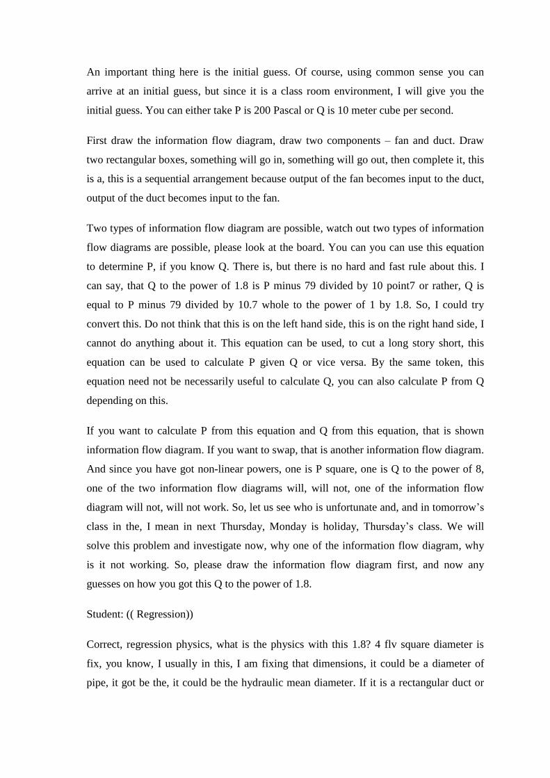
(Refer Slide Time: 42:25)
So, head… So, this dynamic, what about its f itself?
V square multiplied by v square multiplied by v to the power of, so what is it given, 1.8.
What is this fellow doing? Static. So, using regression you can get that. So, I want it
appreciate the physics behind this equation. This equation we cannot get it from physics,
somebody, the manufacturer has to do the experiments, you will give it as a manufacture,
in the manufacturer’s catalogue. It is called the fan characteristics in turbo-machinery.
You must have studied, that pump characteristics, blower, axial fan characteristics,
blower characteristics, turbine characteristics, they have to give, this is the fundamental
experiment they have to do and give, give to the user.
Now, go ahead and first, Vikram do not start solving, information flow diagram started,
then proceed. If you finish the information flow diagram, you can start with the solution.
I will draw the information flow diagram and stop with that today’s class. This problem
will take half an hour for you to solve because even if you get the right answer I want
you to take other answer, information flow diagram and proceed to a point at which it
will cup. So now, I will draw the information flow diagram.
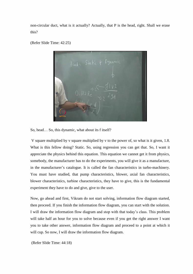
(Refer Slide Time: 44:18)
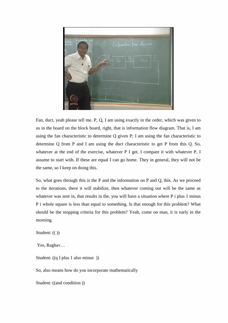
Fan, duct, yeah please tell me. P, Q, I am using exactly in the order, which was given to
us in the board on the block board, right, that is information flow diagram. That is, I am
using the fan characteristic to determine Q given P; I am using the fan characteristic to
determine Q from P and I am using the duct characteristic to get P from this Q. So,
whatever at the end of the exercise, whatever P I get, I compare it with whatever P, I
assume to start with. If these are equal I can go home. They in general, they will not be
the same, so I keep on doing this.
So, what goes through this is the P and the information on P and Q, this. As we proceed
to the iterations, there it will stabilize, then whatever coming out will be the same as
whatever was sent in, that results in the, you will have a situation where P i plus 1 minus
P i whole square is less than equal to something. Is that enough for this problem? What
should be the stopping criteria for this problem? Yeah, come on man, it is early in the
morning.
Student: (( ))
Yes, Raghav…
Student: ((q I plus 1 also minus ))
So, also means how do you incorporate mathematically
Student: ((and condition ))
So, and, or we can do this. So, sigma, that is good, sigma Q i plus 1, we will put some 10
to the power of minus 6, so that you keep on doing or 10 to the power of minus 4, 4 we
will easily get. So, this look like, you think that is very, this is not the most important
part of problem. You think, that getting the, using the algorithm and getting the solution,
the most important part of the problem, but this is also equally important, because in real
life nobody will tell you what is the stopping criterion is, it is for you to figure out, it is
for you to get convince that you have reached the level at which the solution will not
change.
This level of accuracy is ok. I am comfortable with this level of accuracy, because if you
know what the true value is, you can compare your result with respect to the true value.
And then, if I get 1 percent close to the true value, then I am fine, but when you are
doing CFD competition, when you are doing simulation, the true value is elusive. You do
not know what is the true value? So, you are always, you are always looking at the
difference between successive iterations, but this can mislead, this can mislead you
because it is possible for you to finally, beautifully, converge to a totally stupid answer.
So, convergence is necessity. Once you have reached convergence, it does not
necessarily mean, that you got an accurate solution. Convergence means, with the
present numerical scheme, if you proceed for 100 more iterations, you cannot expect a
significant change in the answer, but whether that the answer itself is correct or not,
convergence will not tell you. So, you have to do additional measure, you will have to
validate your solution.
So, you, you apply your numerical technique to some other solution, some other problem
for which either somebody else has done experiments of a, which analytical solutions are
possible. Then, for that case, after you run through so many iterations, after you
incorporate your stopping criterion, you get a solution, which is exactly the same as what
other people have reported or an analytical solution. Then, you say, for this particular
problem when I apply this stopping criterion my solution work. Therefore, when I apply
to a natural problem for which I do not know what the true solution is, there is no reason
why it should misbehave.
So, we will stop here. So, in the next class in the next class, we will solve this problem,
and then we will use both, information flow diagram. There is only one information flow

diagram, I can draw the other one and then, will go through some iteration, and solve
this. I, as is our practice, I will put it on Excel, and I will also demonstrate it with Ms
Excel.