design and implementation of a wind turbine emulator with
TRANSCRIPT
Design and Implementation of a Wind Turbine Emulator with Extended Dynamic
Characteristics
Saeed Khedri
A Thesis
in
The Department
of
Electrical and Computer Engineering
Presented in Partial Fulfillment of the Requirements
for the Degree of Master of Applied Science at
Concordia University
Montreal, Quebec, Canada
October 2008
© Saeed Khedri, 2008

1*1 Library and Archives Canada
Published Heritage Branch
395 Wellington Street Ottawa ON K1A0N4 Canada
Bibliotheque et Archives Canada
Direction du Patrimoine de I'edition
395, rue Wellington Ottawa ON K1A0N4 Canada
Your file Votre reference ISBN: 978-0-494-45518-0 Our file Notre reference ISBN: 978-0-494-45518-0
NOTICE: The author has granted a nonexclusive license allowing Library and Archives Canada to reproduce, publish, archive, preserve, conserve, communicate to the public by telecommunication or on the Internet, loan, distribute and sell theses worldwide, for commercial or noncommercial purposes, in microform, paper, electronic and/or any other formats.
AVIS: L'auteur a accorde une licence non exclusive permettant a la Bibliotheque et Archives Canada de reproduire, publier, archiver, sauvegarder, conserver, transmettre au public par telecommunication ou par Plntemet, prefer, distribuer et vendre des theses partout dans le monde, a des fins commerciales ou autres, sur support microforme, papier, electronique et/ou autres formats.
The author retains copyright ownership and moral rights in this thesis. Neither the thesis nor substantial extracts from it may be printed or otherwise reproduced without the author's permission.
L'auteur conserve la propriete du droit d'auteur et des droits moraux qui protege cette these. Ni la these ni des extraits substantiels de celle-ci ne doivent etre imprimes ou autrement reproduits sans son autorisation.
In compliance with the Canadian Privacy Act some supporting forms may have been removed from this thesis.
Conformement a la loi canadienne sur la protection de la vie privee, quelques formulaires secondaires ont ete enleves de cette these.
While these forms may be included in the document page count, their removal does not represent any loss of content from the thesis.
Canada
Bien que ces formulaires aient inclus dans la pagination, il n'y aura aucun contenu manquant.

ABSTRACT
Design and Implementation of a Wind Turbine Emulator with Extended Dynamic
Characteristics
Saeed Khedri
The wind turbine emulator (WTE) is of concern due to the fact that the wind
energy conversion system (WECS) is a growing industry and needs further improvement.
It is a key component of a test bench which provides the opportunity to investigate the
effect of wind turbine parameters and characteristics on the system responses by
modeling the wind turbine and the drive train. Several WTEs have been proposed by the
researchers with different capabilities and degrees of complexity. The most important
factors which have significant impact on the dynamic behavior of the WECS, as
considered in the literature, are the wind turbine mass moment of inertia, system's natural
frequency, pulsating (oscillatory) torque, and damping constant. In general, at least the
effect of one of these facts was not included or not discussed in the reported WTEs.
This Thesis addresses this problem while considering on a simplified model of a
wind turbine which consists of a mass moment inertia (rotor and hub), a low speed side
flexible shaft, an ideal gearbox, a high speed side rigid shaft, and an electric generator.
The effect of the oscillatory torque is also considered in the model. The simulation results
indicate that the simplified model of the wind turbine and the drive train allow the
investigation of the above mentioned factors on the system responses. It also shows the
iii

different ways of exciting the system's mechanical mode. A 2-hp experimental set-up is
implemented and tested with a dynamometer as a mechanical load and also with a self-
excited induction generator operating in the regulated and unregulated stand-alone mode.
The experimental results agree with the simulation results.
IV

ACKNOWLEDGMENTS
The author has received much advice in completion of this study, but some have
to be singled out for their special contributions which will be memorable for the years to
come.
The author would like to express his sincere gratefulness to his supervisor, Dr.
Luiz A. C. Lopes for his extremely useful guidance, advice, willingness to teach,
friendship, and financial support throughout this study period.
The author would like to thank Dr. Pragasen Pillay and Dr. Sheldon Williamson
for their excellent suggestions. Special thanks to Mr. Joseph Woods for his excellent
technical and practical suggestions, friendship and great help.
The author would also like to thank his colleagues in the P. D. Ziogas Power
Electronics Laboratory, Messrs Niel S. D'Souza, Yongzheng Zhang, Reinaldo Tonkoski,
Maged Barsom, Ghulam Dastagir, and Nayeem Ahmed Ninad for their great suggestions
and invaluable friendships.
Last but not least, the author is very grateful towards his family for their
encouragement and support which made it possible to complete this study.
v

To my family
VI

TABLE OF CONTENTS
List of Figures xi
List of Tables xv
List of Acronyms xvi
List of Principal Symbols xvii
CHAPTER 1 1
Introduction 1
1.1 Background 1
1.2WECSs 5
1.2.1 Terminologies 5
1.2.2 Main Components 7
1.2.3 General Classification 7
1.3 Thesis Scope and Contributions 11
1.4 Thesis Outline 13
CHAPTER 2 15
Modeling and simulation of a wind turbine emulator 15
2.1 Introduction 15
2.2 Rotor (Wind Wheel) [3] 16
2.2.1 Power Coefficient (Cp) 16
vii
2.2.2 Torque-Speed and Power- Speed Characteristics 18
2.2.3 Oscillatory Torque 22
2.3 Drive Train 24
2.3.1 Natural Frequencies 26
2.3.2 Shaft Torsional Spring and Damping Constants 29
2.4 WECS Differential Equations and Block Diagram 30
2.5 Simulation of WECS 32
2.5.1 MATLAB/Simulink Model 32
2.5.2 Parameters Selection 33
2.5.3 Simulation Results 35
2.6 Conclusions 45
CHAPTER 3 47
Design and Implementation of a WTE 47
3.1 Introduction 47
3.2 PMDC Machines 48
3.2.1 Model and Characteristics [24, 25] 49
3.2.2 PMDC Machine Parameters 51
3.3 Power Electronics and Controllers 53
3.3.1 Line-Frequency Controlled Converters [24] 53
3.3.2 Switch-Mode DC-DC Converters [24] 55
3.4 Control Logic of the WTE [6] 58
viii
3.5 Experimental Set-up 60
3.6 Experimental Results 77
3.7 Conclusions 90
CHAPTER 4 91
An Application of the WTE 91
4.1 Introduction 91
4.2 Induction Generator Model, Parameters, and Characteristics [30, 31] 93
4.3 Experimental Set-Up 96
4.3.1 WTE Parameters Selection 96
4.3.2 MATLAB/Simulink Model 98
4.3.3 Power Measurement Block 100
4.4 Experimental Results 101
4.4.1 Unregulated WECS 102
4.4.2 Regulated WECS 121
4.5 Conclusions 128
CHAPTER 5 130
Conclusions 130
5.1 Summary 130
5.2 Suggestions for Future Work 132
References 134
ix

Appendices 138
Appendix A: Relation Between the Wind Speed and Operating Point on the Wind
Turbine Characteristic 138
Appendix B: Electronics circuit for Switches Gating Signals 139
X
LIST OF FIGURES
Fig. 1-1 ATypical horizontal axis wind turbine 6
Fig. 1-2 General classification of WECSs 8
Fig. 1-3 Typical grid-connected WECSs configurations [5] 9
Fig. 2-1 Simplified schematic diagram of a stand-alone WECS 16
Fig. 2-2 Air flow conditions as a result of mechanical energy extraction from a free-Stream air flow based on the elementary momentum theory [3] 17
Fig. 2-3 Torque coefficient (Ct) versus tip speed ratio (2.) Curve [6] 19
Fig. 2-4 Torque-speed characteristic of the rotor 21
Fig. 2-5 Power-speed characteristic of the rotor 21
Fig. 2-6 Tower shadow and wind shear effects; (a) Produced torque by each blade; (b) Total produced torque when all blades have the same performance [17] 24
Fig. 2-7 A 2-mass system; (a) actual configuration; (b) equivalent configuration for calculating natural frequency when generator rotates at a constant speed 27
Fig. 2-8 Mesh analogy of Fig. 2-7(a) 28
Fig. 2-9 Shaft with length lsh and radius rsh [19] 29
Fig. 2-10 WECS model [6] 31
Fig. 2-11 Block diagram of WECS model [6, 23] 32
Fig. 2-12 MATLAB/Simulink model of WECS 33
Fig. 2-13 Simulation results for case 1 36
xi

Fig. 2-14 Simulation results for case 2 37
Fig. 2-15 Simulation results for case 3 38
Fig. 2-16 Simulation results for case 4 40
Fig. 2-17 Simulation results for case 5 42
Fig. 2-18 Simulation results for case 6 44
Fig. 3-1 PMDC machine equivalent circuit in motoring operation 49
Fig. 3-2 PMDC motor model [25] 50
Fig. 3-3 PMDC machine characteristics; (a) Continuous torque-speed capability; (b) torque-speed characteristics for different terminal voltages where vt4 > v« > VQ > vtj [24] 51
Fig. 3-4 Line-frequency controlled converters configuration; (a) 1-quadrant converter; (b) 2-quadrant converter; (c) 4-quadrant converter [24] 54
Fig. 3-5 Control concept of line-frequency controlled converter [24] 55
Fig. 3-6 Switch-mode DC-DC converter configurations; (a) 1-quadrant converter; (b) 2-quadrant converter; (c) 4-quadrant converter [24] 56
Fig. 3-7 Fixed-frequency current control block diagram [24] 56
Fig. 3-8 Tolerance band current control; (a) waveforms and switching concept; (b) control block diagram [24] 57
Fig. 3-9 WTE control logic schematic diagram 59
Fig. 3-10 WTE experimental set-up 61
Fig. 3-11 Equivalent circuit of the prime mover in two operating conditions; (a) Upper switch is on; (b) Lower switch is on 63
Fig. 3-12 Dynamometer speed signal and its frequency spectrum 66
xii
Fig. 3-13 Block diagram for creating actually modified speed signal 68
Fig. 3-14 Input/output signals to and from dSPACE ds-1103 control board 72
Fig. 3-15 MATLAB/Simulink model for implementation of the experimental set-up 74
Fig. 3-16 Prime mover hysteresis current controller model 76
Fig. 3-17 Experimental results for case 1; (a) WTE responses; (b) Zoom of the
dynamometer speed signals 79
Fig. 3-18 Experimental results for case 2; (a) WTE responses; (b) Zoom of the dynamometer speed signals 81
Fig. 3-19 Experimental results for case 3; (a) WTE responses; (b) Zoom of the dynamometer speed signals 83
Fig. 3-20 Experimental results for case 4; (a) WTE responses; (b) Zoom of the
dynamometer speed signals 85
Fig. 3-21 Experimental results for case 5 87
Fig. 3-22 Experimental results for case 6 89
Fig. 4-1 Unregulated electric power generation using WTE 91
Fig. 4-2 Regulated electric power generation (Stand-Alone) using WTE 92
Fig. 4-3 Simplified model of an induction machine [31] 94
Fig. 4-4 Induction machine characteristics; (a) Frequency versus speed characteristic; (b) Air-gap line voltage versus speed characteristic [30] 95
Fig. 4-5 MATLAB/Simulink model for implementation of the experimental set-up 99
Fig. 4-6 Modified MATLAB/Simulink (version 5.3) power measurement block 101
Fig. 4-7 Unregulated WECS experimental results for case 1 by method-A 104
xiii

Fig. 4-8 Unregulated WECS experimental results for case 1 by method-B 105
Fig. 4-9 Unregulated WECS experimental results for case 2 by method-A 109
Fig. 4-10 Unregulated WECS experimental results for case 2 by method-B 110
Fig. 4-11 Unregulated WECS experimental results for case 3; (a) By method-A, Bsh = 0.7307 Nms/rad; (b) By method-A, Bsh = 2 Nms/rad; (c) By method-B 112
Fig. 4-12 Unregulated WECS experimental results for case 4; (a) By method-A; (b) By method-B 114
Fig. 4-13 Unregulated WECS experimental results for case 5 (Jwt = 3 kgm ); (a) By method-A; (b) By method-B 116
Fig. 4-14 Unregulated WECS experimental results for case 5 (Jwt = 7 kgm2); (a) By method-A; (b) By method-B 117
Fig. 4-15 Unregulated WECS experimental results for case 6 (Jwt = 3 kgm2); (a) By method-A; (b) By method-B 119
Fig. 4-16 Unregulated WECS experimental results for case 6 (Jwt = 7 kgm2); (a) By
method-A; (b) By method-B 120
Fig. 4-17 Regulated WECS experimental results for case 1 (Jwt = 3 kgm2); (a) By method-A; (b) By method-B 123
Fig. 4-18 Regulated WECS experimental results for case 1 (Jwt = 7 kgm2); (a) By method-A; (b) By method-B 124
Fig. 4-19 Regulated WECS experimental results for case 2 (Jwt = 3 kgm2); (a) By method-A; (b) By method-B 126
Fig. 4-20 Regulated WECS experimental results for case 2 (Jwt = 7 kgm2); (a) By method-A; (b) By method-B 127
Fig. B-l Electronic circuit for creating gating signals for the switches 139
XIV

LIST OF TABLES
Table 1-1 Summary of comparison between proposed WTEs 11
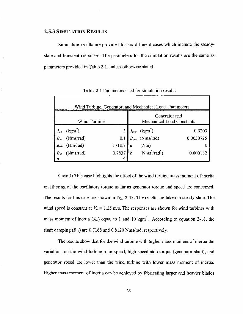
Table 2-1 Parameters used for simulation results 35
Table 3-1 PMDC machine rating and parameters 52
Table 4-1 Parameters of the induction machine [30] 94
Table 4-2 Parameters used for experimental results 102
XV

LIST OF ACRONYMS
AC
ADC
BJT
DAC
DC
DSP
emf
FFT
hp
IGBT
KVL
kW
MOSFET
PI
PMDC
PMSG
SCIG
VSI
WECS
WRIG
WTE
Alternating Current
Analogue to Digital Converter
Bipolar Junction Transistor
Digital to Analogue Converter
Direct Current
Digital Signal Processor
Electro-Motive Force
Fast Fourier Transform
Horse Power
Insulated-Gate Bipolar Transistor
Kirchhoff s Voltage Law
Kilo Watt
Metal-Oxide-Semiconductor Field-Effect-Transistor
Proportional Integral
Permanent Magnet Direct Current
Permanent Magnet Synchronous Generator
Squirrel-Cage Induction Generator
Voltage Source Inverter
Wind Energy Conversion System
Wound Rotor Induction Generator
Wind Turbine Emulator

LIST OF PRINCIPAL SYMBOLS
A
"gen
Bsh
Bwt
C
Q
Cp
eb
fn
G
Jgen
Jsh
Jwt
Kb
Ksh
K,
L
La
X
n
•* dyn
Wind Turbine Rotor Swept Area (m2)
Generator Damping Constant (Nms/rad)
Shaft Damping Constant (Nms/rad)
Wind Turbine Damping Constant (Nms/rad)
Capacitance (F)
Wind Turbine Rotor Torque Coefficient (-)
Wind Turbine Rotor Power Coefficient (-)
PMDC Machine Back emf (V)
Natural Frequency (Hz)
Shear Modulus (Pa)
Generator Mass Moment of Inertia (kgm2)
Shaft Polar Moment of Inertia (m4)
Wind Turbine Mass Moment of Inertia (kgm2)
PMDC Machine Speed Constant (Vs/rad)
Shaft Torsional Spring Constant (Nm/rad)
PMDC Machine Torque Constant (m/A)
Inductance (H)
PMDC Machine Armature Inductance (H)
Tip Speed Ratio (-)
Gear Box Ratio (-)
Dynamometer Power (W)
•» g e n
•• w t
R
Ra
Rr
Rs
P
*hs
Tload
?ls
Tref
T\vt_av
9sh
vw
Oidyn
COgen
COwt
(On
c Csh
Generator Power (W)
Wind Turbine Power (W)
Wind Turbine Rotor Radius (m)
PMDC Machine Armature Resistance (£2)
Induction Machine Rotor Resistance (Q.)
Induction Machine Stator Resistance (Q)
Air Density (kg/m )
High Speed Side Shaft Torque (Nm)
Load Torque (Nm)
Low Speed Side Shaft Torque (Nm)
Refernce (High Speed Side Shaft) Torque (Nm)
Wind Turbine Rotor Average Torque (Nm)
Shaft Twist Angle (rad)
Wind Speed (m/s)
Dynamometer Rotational Speed (rad/s)
Generator Rotational Speed (rad/s)
Wind Turbine Rotor Rotational Speed (rad/s)
Natural Frequency (rad/s)
Second Order Low Pass Filter Damping Factor (-)
Shaft Damping Ratio (-)
XVlll

CHAPTER 1
INTRODUCTION
1.1 BACKGROUND
The interest for renewable sources of energy or in other words, green power, is
drastically increasing worldwide. The main reasons are the green house effect and
tendency towards less dependency on natural resources such as oil and coal. Researchers
are working on renewable energy conversion systems to make them more cost effective,
more environmentally friendly, and more reliable. The major renewable sources of
energy can be listed as Biomass, Geothermal, Solar, and Wind [1].
Biomass is basically plant matter or any kind of biological material. It can be used
for generating electricity with reduced greenhouse gas emissions in comparison with
generating electricity using fossil fuel. Generating electricity by using biomass is called
biomass power. Based on the method of using of biomass in generating electricity the
technology can be categorized as: direct-firing, co-firing, gasification (high temperature
environment with limited oxygen), pyrolysis (pyrolyzing biomass in the absence of
oxygen), and anaerobic digestion (decomposing organic matter in a closed reactor
without oxygen) [1].
Geothermal relates to the heat from the earth due to the hot water or stream in the
earth. They can be accessed by drilling and be used for generating electricity instead of
using fossil fuel. There are mainly three ways of using geothermal for producing
electricity. They are dry steam, flash steam, and binary cycle. In dry steam, the steam is
piped from the wells, which are dug to reach the hot water, to a power plant with steam
1

turbines. In flash steam, the very hot water rises through the well. Near the surface, as the
pressure decreases, some of them turn to steam. The steam is separated from the water
and used for turning the steam turbine. In the binary cycle, the heat of hot water is used to
boil an organic compound (low boiling point) which will be used for turning a turbine
Solar technologies concentrate on capturing energy from the sun. It is used for
producing electricity in two general forms, concentrating solar power and solar cells
(photovoltaic). The main types of concentrating solar power systems are: parabolic-
trough (use of mirrors for concentrating solar energy on to the pipes with flowing oil
which is used for boiling water), dish/engine (use of mirrors which concentrate the sun's
energy on the fluid within the engine; expansion of the fluid produces mechanical
power), and power tower (use of mirrors which concentrate the sun's energy on top of the
tower, which heats the molten salt and its heat is used for boiling water). The solar cells
(photovoltaic or PV) convert the sun's light directly into electricity. They can be used in
arrays to form higher power electric generation [1].
A wind energy system is based on the capture of energy from moving air particles
and its conversion into rotating (mechanical) power. There are different ways of
capturing wind energy which are called wind turbines. The most popular one is horizontal
axis wind turbine with 2 or 3 blades [1].
Each of above mentioned systems are a vast area and currently many researchers
with the collaboration of industries and governments are working on them. Wind energy
system is one of the fastest-growing renewable energy and the installed wind energy
systems are increasing [1,2].
2

In general, mechanical rotation which is created by capturing wind energy can be
used in different ways. Wind-mills and wind-wheels are two types of WECS which have
been used by mankind since long time ago for milling grains and pumping water,
respectively [3].
The other way of using wind energy is to convert the captured energy into
electricity. Environmental concerns and technological developments in the areas of
power electronics, electric machines, and control have made possible the conversion of
wind energy into electricity, in a cost-effective way. Nowadays, wind energy conversion
systems (WECSs) — this terminology will be used for the systems which convert wind
energy to electricity— are available in the capacity range of fraction of kW for residential
application and hundreds of MW in the form of wind farms [3]. Thus, this Thesis focuses
on WECSs and is organized in a way to highlight the important facts in this technology
which will affect the quality of the generated electricity.
WECS as a new technology needs a great deal of research works. These can be
split in mechanical and electrical research works to improve the performance of the
systems such as efficiency, cost, and reliability. For these reasons it is necessary to
investigate the effect of system parameters on its overall performance, to select suitable
configuration for generating electricity, and to choose the most effective control strategy
for a given system. Thus, the question is about the possible ways to perform the tests.
One option is to build the designed WECS and test different configurations and
control techniques in generating electricity. This would be a good idea in a sense, that is,
the researchers will be working on the real system. But there are few drawbacks which
make it impossible for most researches. First, building the real system would be very
3

costly and time consuming. Second, once the system is built, varying each system
parameter is impractical. Third, the system has to be tested in a field which in this case,
there would be no control on wind speed and wind gusts since the wind speed variations
is random. Therefore, it is not possible to study the impact of each system parameter
individually.
The second option is to use the built system in a wind tunnel. This will solve the
problem of non-controllable environment in the terms of having randomly variations on
the wind speed, but it brings up other issues in addition to the first two issues that exist
for the first option. The first issue is that, wind tunnel itself is costly. The second is due to
the dimensions of the wind tunnel. This limits the size and capacity of the WECS which
needs to be tested.
The third option [4] is to select and use a prime mover plus a flywheel, which
represents the wind turbine mass moment of inertia, and the remaining parts such as
shafts, gearbox, and the generator remain the same as the wind turbine which will be
emulated. The main drawbacks of this type of wind turbine emulator (WTE) are briefly
discussed below. First, the prime mover must be able to operate with high torque and low
speed (this is true as the size of the wind turbine rotor increases). Second, since the major
parts of the wind turbine are not modeled, it will not be easy to change the parameters to
investigate their impacts on the system responses. The advantage of this WTE is that it
provides a control over wind speed change, since it is modeled.
The last option, which is the aim of this Thesis, is to develop a simple model of
the wind turbine rotor and the drive train and use it with the wind speed as the input
reference for the torque developed by a wind turbine emulator. The idea is to simulate the
4
model of the wind turbine and control an electric motor as prime mover to follow the
reference signals, for instance, torque created by the model. This can be done by using a
real-time software as interface to communicate between the model and the system set-up.
Since the wind turbine is modeled, the parameters can be set to different values to find
out their impacts on the system outputs in transient and steady-state responses. Besides,
since the wind speed is defined as an input within the model, it can be varied at will.
Furthermore, as the prime mover runs a generator, the load at the output of the generator
can be varied to study the impact of the load variations in the transient and steady-state
responses.
1.2 WECSS
1.2.1 T E R M I N O L O G I E S
In this section some basic terminologies of WECs are described which are useful
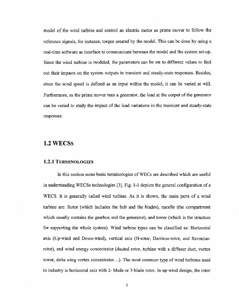
in understanding WECSs technologies [3]. Fig. 1-1 depicts the general configuration of a
WECS. It is generally called wind turbine. As it is shown, the main parts of a wind
turbine are: Rotor (which includes the hub and the blades), nacelle (the compartment
which usually contains the gearbox and the generator), and tower (which is the structure
for supporting the whole system). Wind turbine types can be classified as: Horizontal
axis (Up-wind and Down-wind), vertical axis (H-rotor, Darrieus-rotor, and Savonius-
rotor), and wind energy concentrator (ducted rotor, turbine with a diffuser duct, vortex
tower, delta wing vortex concentrator...). The most common type of wind turbines used
in industry is horizontal axis with 2- blade or 3-blade rotor. In up-wind design, the rotor
5

is on the windward and in down-wind design; it is on the leeward of the tower. In up
wind
NACELLE
TOWER
/////////
Fig. 1-1A Typical horizontal axis wind turbine
design the nacelle has to have yaw mechanism to keep the rotor facing the wind direction
This mechanism may not be needed for downwind wind turbines by proper design of the
rotor and nacelle in such a way that the nacelle follows the wind passively. This is one of
the advantages of downwind design, but in practice it can be used for wind turbines up to
a certain capacity. Its other advantage is that it allows the use of more flexible blades,
which in turn will be lighter and help the structural dynamics of the wind turbine. The
disadvantage of down-wind designs is the pulsations in generated power, which happens
every time each rotor blade passes in front of the tower. This causes more fatigue load on
mechanical parts with respect to the up-wind design.
Since in WECSs, the rotor speed is usually lower than the required rotor speed at
the generator, a gearbox is used. Low speed side expression is used for the components
from the rotor to the gearbox. Similarly, high speed side expression is used for the
6

components from the gearbox to the generator. The other terminology is the blade pitch
angle. It is related to the aerodynamics of blades and wind direction. The concept is that
by changing the pitch angle the amount of power which is captured from wind can be
controlled.
1.2.2 MAIN COMPONENTS
The main components of WECS which have significant impacts in the generated
electricity are listed below.
Rotor: This mainly includes the hub and the blades. The main portion of total
mass moment of inertia of wind turbines is due to the rotor as mentioned in the literature.
Drive train: It generally includes the low speed side shaft, gearbox, and the high
speed side shaft.
Electric generator: The most popular electric generators in WECS industry are
asynchronous and synchronous generators. The most common types of the generators are
introduced in section 1.2.3.
Power electronics devices: This in general includes soft starters and different
types of converters. Some of the configurations of the power electronics devices are
introduced in section 1.2.3.
1.2.3 GENERAL CLASSIFICATION
With the ever-increasing advancement of power electronics different
classifications of WECSs have been offered and tested by researchers and manufacturers
7

and there would be more to offer. WECSs can be classified based on the different
concepts. Fig. 1-2 shows a general classification of WECSs. Each category is briefly
described below.
Rotor speed concept [5]: It generally includes two types: Constant speed and
variable speed. In the constant speed concept, the wind turbine the rotor rotates at
constant speed independently of the load conditions. The wind speed determines how
much power the wind turbine can produce. In the variable speed concept, as the wind
speed changes the wind turbine rotor turns at different speed to produce its maximum or
close to maximum power.
Constant-Speed
Variable-Speed
Stall Control
Pitch Control
Active Stall Control
Grid-Connected
Sliind-'Mnnc
Fig. 1-2 General classification of WECSs
Power control concept [5]: It can be categorized in three general cases: Stall
control, pitch control, and active stall control. In the stall (passive) control, the blades are
aerodynamically designed in a manner that for the wind speeds higher than a certain
8
value the power captured by the blades reduces and for higher than another certain value
the blades captures no power (stall). In the pitch control concept, by pitching the blades
(turning them into or out of the wind) the amount of the power captured by the blades
will be controlled. In the active stall control, both concepts, which are stall and pitch
control, are used in the design of the wind turbine rotor.
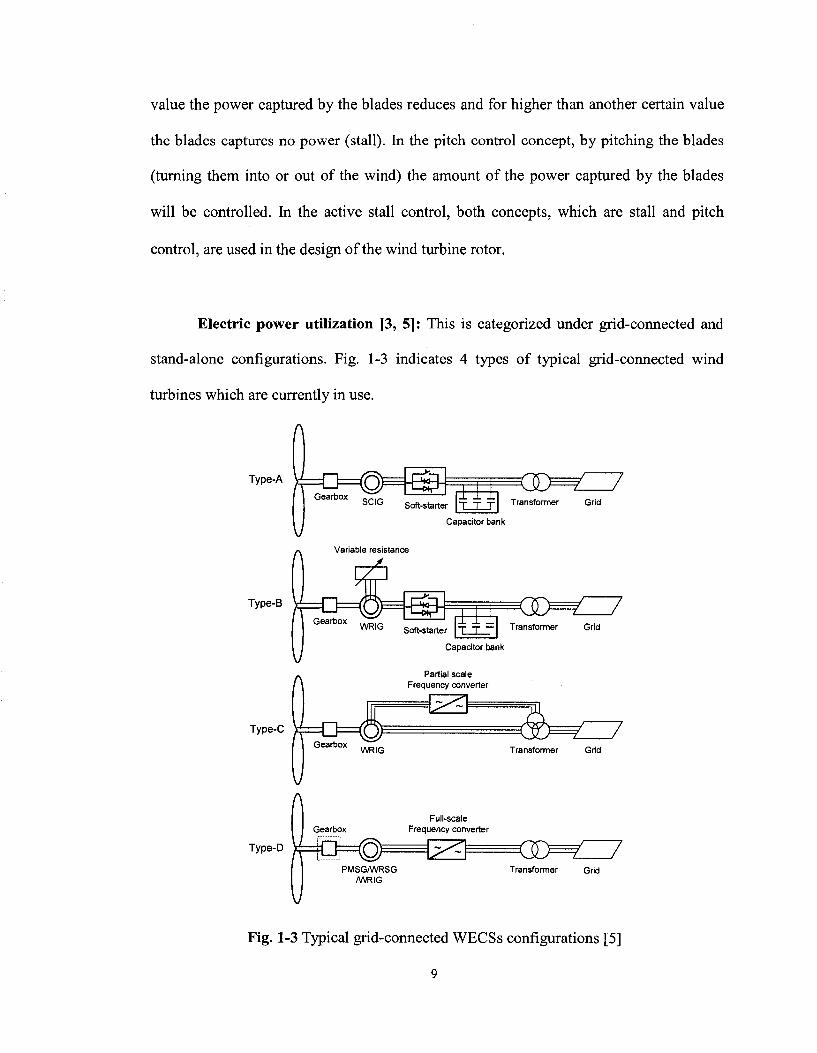
Electric power utilization [3, 5]: This is categorized under grid-connected and
stand-alone configurations. Fig. 1-3 indicates 4 types of typical grid-connected wind
turbines which are currently in use.
A
Type-A ^ C H O ^ S -' ! Gearbox ' ' SCIG Soft-starter Transformer Grid
Capacitor bank
Variable resistance y
Type-B
WRIG soft-starter T T T Transformer Grid
Capacitor bank
Partial scale Frequency converter
Type-C V ^ O Gearbox
1=0 7 WRIG Transformer Grid
Type-D
Full-scale Frequency converter
<3>^Z7 Transformer Grid
Fig. 1-3 Typical grid-connected WECSs configurations [5]
9
Type-A is a constant speed configuration. It is the most common and rugged
configuration. A squirrel cage induction generator (SCIG) is used as the generator. Type-
B is a limited variable speed configuration. The generator is a wound rotor induction
generator (WRIG). The slip of induction generator is controlled by varying the variable
resistor which is in series with rotor winding. Type-C is also a limited variable speed
configuration. It includes a WRIG and a partial frequency converter. This is also called
doubly fed induction generator (DFIG). The converter controls the speed (for a limited
range) by controlling the rotor reactive power and also used for the smooth connection to
the grid. Type-D is a variable speed configuration for a wide range by using a full-scale
frequency converter. The generator types could be wound rotor synchronous generator
(WRSG), WRIG, or permanent magnet synchronous generator (PMSG). In some cases
the gearbox is eliminated by using a multi-pole generator [5].
In a stand-alone WECS, since wind is not available at all times, for continuous
power generation, it has to be equipped with energy storage system and it may also be
backed up, for instance, with diesel-engine electric power generation. There are different
applications for stand-alone WECSs such as residential heating, pumping water, and
desalination of sea water [3]. There are also different schemes and control strategies
based on the type of the applications for stand-alone operation of WECSs in which power
electronics converters play an important role. An available stand-alone scheme is
introduced in Chapter 4.
10
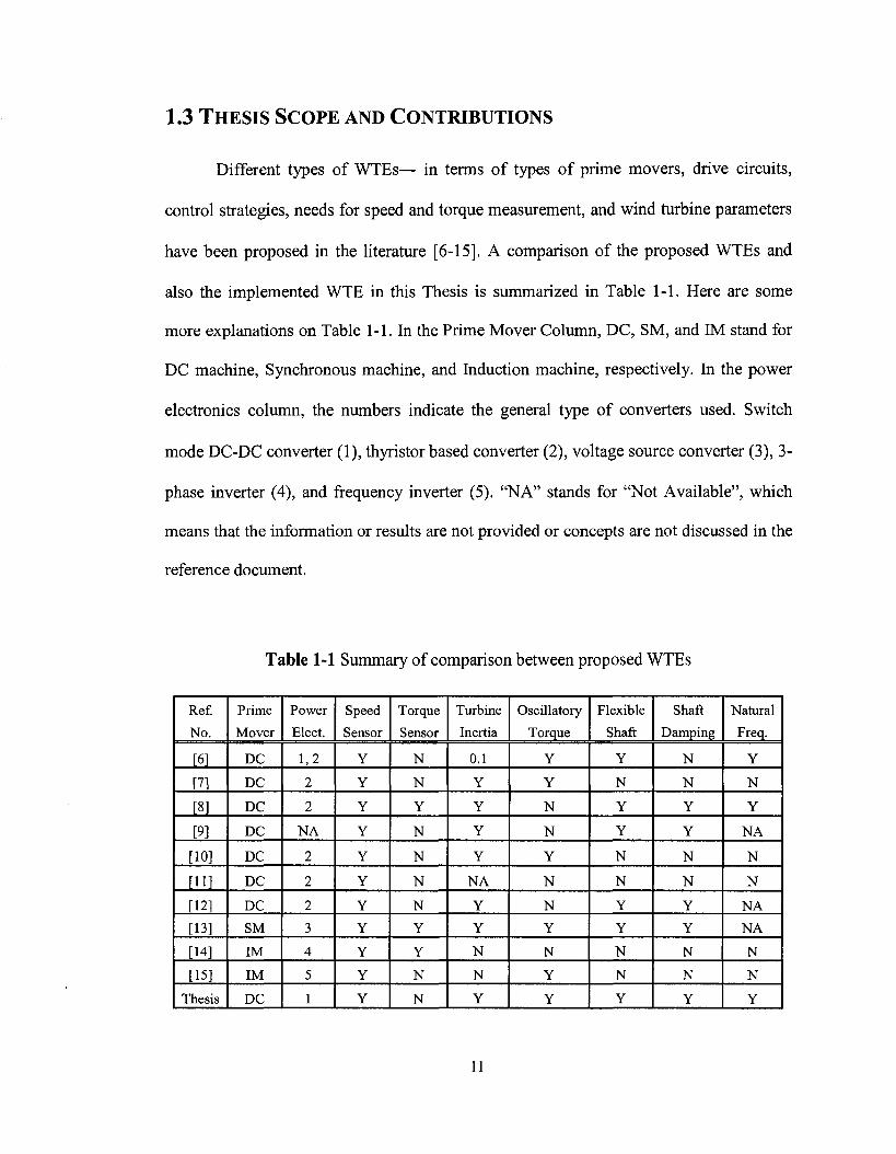
1.3 THESIS SCOPE AND CONTRIBUTIONS
Different types of WTEs— in terms of types of prime movers, drive circuits,
control strategies, needs for speed and torque measurement, and wind turbine parameters
have been proposed in the literature [6-15]. A comparison of the proposed WTEs and
also the implemented WTE in this Thesis is summarized in Table 1-1. Here are some
more explanations on Table 1-1. In the Prime Mover Column, DC, SM, and IM stand for
DC machine, Synchronous machine, and Induction machine, respectively. In the power
electronics column, the numbers indicate the general type of converters used. Switch
mode DC-DC converter (1), thyristor based converter (2), voltage source converter (3), 3-
phase inverter (4), and frequency inverter (5). "NA" stands for "Not Available", which
means that the information or results are not provided or concepts are not discussed in the
reference document.
Table 1-1 Summary of comparison between proposed WTEs
Ref.
No.
[6]
[7]
[8]
[9]
[10]
[11]
[12]
[13]
[14]
[15]
Thesis
Prime
Mover
DC
DC
DC
DC
DC
DC
DC
SM
IM
IM
DC
Power
Elect.
1,2
2
2
NA
2
2
2
3
4
5
1
Speed
Sensor
Y
Y
Y
Y
Y
Y
Y
Y
Y
Y
Y
Torque
Sensor
N
N
Y
N
N
N
N
Y
Y
N
N
Turbine
Inertia
0.1
Y
Y
Y
Y
NA
Y
Y
N
N
Y
Oscillatory
Torque
Y
Y
N
N
Y
N
N
Y
N
Y
Y
Flexible
Shaft
Y
N
Y
Y
N
N
Y
Y
N
N
Y
Shaft
Damping
N
N
Y
Y
N
N
Y
Y
N
N
Y
Natural
Freq.
Y
N
Y
NA
N
N
NA
NA
N
N
Y
In [6], the WTE has been tested with 2 types of converters for comparison, but in
both cases the maximum wind turbine inertia was equal to 0.1 kgm . In [8], the values for
system parameters such as wind turbine mass moment of inertia, shaft torsional spring
and damping constants were not provided. In [13], a speed sensor is used but it is not
mentioned if it is used for just monitoring purpose or used as part of control strategy.
In this Thesis, the proposed WTE consists of a model of the wind turbine, for
generating the reference torque at the high speed side, a permanent magnet DC (PMDC)
machine as prime mover and a switch-mode DC-DC converter with hysteresis current
controller. The main concern in this research work is to show the effect of system
parameters on the system responses. The proposed WTE is able to show the effect of the
wind turbine mass moment of inertia on filtering of the wind speed variations and also
torque pulsations. Effect of load variations on the system responses are verified by using
a dynamometer in one case and an electric generator in another case. It also includes a
flexible shaft in drive train which makes it possible to investigate the possibilities of
mechanical resonance occurrence. In addition to these, two harmonics (1st and 3rd with
respect to rotor speed) are added as torque pulsations to the average torque rotor, due to
tower shadow effect and wind shear effect, and their effects are investigated.
The following are the main contributions of this Thesis:
1) Modeling of WECSs and selection of parameters that would be used as an
unregulated wind turbine as prime mover for stand-alone or grid-connected applications.
2) Implementation of a 2-hp WTE. A PMDC machine is used as dynamometer.
This allows imposing mechanical load on the prime mover without having an electric
generator and variable electric load, to make the emulated wind turbine operates with
12
different loads. It also allows studying the impact of the wind speed variations, load
variations and the wind turbine parameters on the system responses.
3) Applying the WTE prototype in a test bench for an available stand-alone
electric generating set, consisting of voltage source inverter (VSI), SCIG, and PI
controllers which were designed to regulate the generated voltage and frequency of a
generator, connected to an unregulated prime mover. It provides a good opportunity to
study the effect of wind turbine parameters, for instance, impact of the wind turbine mass
moment of inertia on selection of PI controller gain coefficients.
1.4 THESIS OUTLINE
This Thesis is presented in 5 Chapters.
The first Chapter describes the WECS, its growth, and consequently the need for a
WTE. It also briefly introduces the works that have been done and finally covers the
scope and contribution of this Thesis.
The second Chapter presents the differential equations governing a WECS and a
model to be simulated in MATLAB/Simulink. Simulation results are presented to indicate
the effect of system parameters, individually and as a whole, wind speed variations and
load variations on the system responses.
The third Chapter introduces the method of implementing a WTE. In this method,
a permanent magnet DC machine (PMDC) is used as prime mover and another is used as
dynamometer which behaves as a controllable mechanical load. The characteristics of the
PMDC are presented. The controller and selection of the system parameters for
experimental set-up are discussed. The real-time software dSPACE/ControlDesk and its
13

digital controller board (ds-1103) used for implementation of the WTE are briefly
introduced. The experimental results are provided to show the system behavior and
responses for different system parameters due to wind speed and load variations.
The fourth Chapter shows the application of the implemented WTE in Chapter
three, where the dynamometer is replaced by a SCIG connected to variable electrical
load. In this Chapter the characteristics of SCIG are described. The WTE set-up and the
necessary rearrangements for applying it in an unregulated WECS are presented. Then,
the available regulated electric generation set-up (as a stand-alone application of WECSs)
for testing the implemented WTE is discussed. The experimental results are presented to
show the effectiveness of the WTE in electric power generation applications.
The Fifth Chapter concludes the work and highlights the contribution of this
Thesis. In the end, suggestions for future work are presented.
14
CHAPTER 2
MODELING AND SIMULATION OF A WIND TURBINE EMULATOR
2.1 INTRODUCTION
The first step in designing a wind turbine emulator (WTE) is the selection of its
features which depend on the studies to be carried out with the WTE. For the analysis of
the impact of load and wind speed variations in the steady state value of the shaft speed
and consequently frequency of a stand-alone wind energy conversion system (WECS),
the WTE could be simply a motor with a torque control loop. The reference torque varies
with the shaft speed, wind speed and torque speed characteristics of the wind rotor. The
WTE to be developed in this thesis is intended to be used in the study of the transient
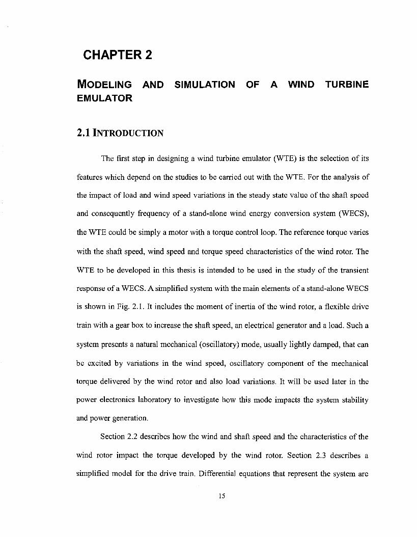
response of a WECS. A simplified system with the main elements of a stand-alone WECS
is shown in Fig. 2.1. It includes the moment of inertia of the wind rotor, a flexible drive
train with a gear box to increase the shaft speed, an electrical generator and a load. Such a
system presents a natural mechanical (oscillatory) mode, usually lightly damped, that can
be excited by variations in the wind speed, oscillatory component of the mechanical
torque delivered by the wind rotor and also load variations. It will be used later in the
power electronics laboratory to investigate how this mode impacts the system stability
and power generation.
Section 2.2 describes how the wind and shaft speed and the characteristics of the
wind rotor impact the torque developed by the wind rotor. Section 2.3 describes a
simplified model for the drive train. Differential equations that represent the system are
15
derived in Section 2.4 and a number of simulations are carried out in section 2.5 with
MATLAB/Simulink to verify if the selected simplified model allows the study of the
mechanical modes of a WECS.
V
\:N
I
LOAD
<#wt
p U u b = ^ -r,-\
Generator
ZL
Z L
z L
Fig. 2-1 Simplified schematic diagram of a stand-alone WECS
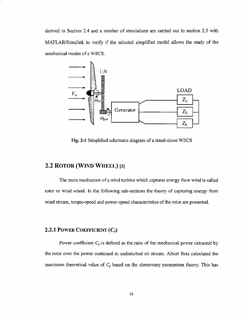
2.2 R O T O R ( W I N D W H E E L ) [3]
The main mechanism of a wind turbine which captures energy from wind is called
rotor or wind wheel. In the following sub-sections the theory of capturing energy from
wind stream, torque-speed and power-speed characteristics of the rotor are presented.
2.2.1 POWER COEFFICIENT (CP)
Power coefficient Cp is defined as the ratio of the mechanical power extracted by
the rotor over the power contained in undisturbed air stream. Albert Betz calculated the
maximum theoretical value of Cp based on the elementary momentum theory. This has
16

been expressed in [3]. A very brief explanation and conclusion of the discussion in [3], is
presented below.
Fig. 2-2 shows the air flow at different stages of an ideal energy conversion
system which is located at plane A'. The energy can be extracted from a free-stream air
flow in the form of kinetic energy. Since the mass must remain unchanged, the velocity
of air flow must be reduced after the energy converter. Therefore, by considering the fact
that mass flow must remain unchanged, according to equation 2-1 the air flow must be
widened in the presence of the energy converter as shown in Fig. 2-2.
m=pVwA (2-1)
Where m is mass flow in kg/s, p is the air density in kg/m , Vw is wind speed in m/s, and
A is the area, which air passes through in m2.
VvA
A\
1 yS
1
- 1
r L — - ~ ^ L Pmech Ai Vw2
Fig. 2-2 Air flow conditions as a result of mechanical energy extraction from a free-
stream air flow based on the elementary momentum theory [3].
The power coefficient is expressed as:
p~ Po " 2 1+ VW2
'wl (2-2)
17
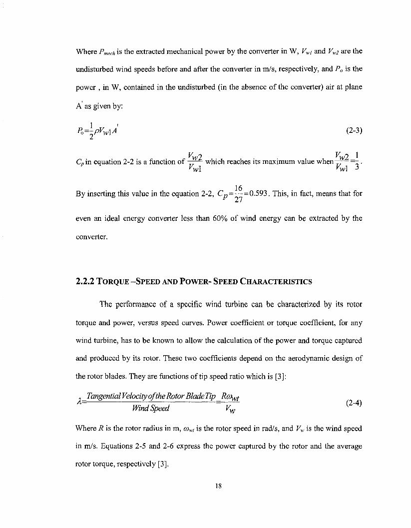
Where Pmech is the extracted mechanical power by the converter in W, Vwj and VW2 are the
undisturbed wind speeds before and after the converter in m/s, respectively, and P0 is the
power , in W, contained in the undisturbed (in the absence of the converter) air at plane
A as given by:
Po=l-pVwXA (2-3)
C„in equation 2-2 is a function of —— which reaches its maximum value when———- . Vw\ Vw\ 3
1 f\ By inserting this value in the equation 2-2, C„=—=0.593. This, in fact, means that for
even an ideal energy converter less than 60% of wind energy can be extracted by the
converter.
2.2.2 T O R Q U E - S P E E D AND P O W E R - S P E E D CHARACTERISTICS
The performance of a specific wind turbine can be characterized by its rotor
torque and power, versus speed curves. Power coefficient or torque coefficient, for any
wind turbine, has to be known to allow the calculation of the power and torque captured
and produced by its rotor. These two coefficients depend on the aerodynamic design of
the rotor blades. They are functions of tip speed ratio which is [3]:
. _Tangential Velocity of the Rotor Blade Tip_RcoWf
Wind Speed Vw
Where R is the rotor radius in m, cowt is the rotor speed in rad/s, and Vw is the wind speed
in m/s. Equations 2-5 and 2-6 express the power captured by the rotor and the average
rotor torque, respectively [3].
18

Pwt=\pCp{X)vlA (2-5)
Where Pwt is the power captured by the rotor in W, CP(X) is rotor power coefficient, p is
the air density in kg/m , and A is the rotor swept area in m .
1 2 T = ^ pC {X)V AR
wt av l t w
(2-6)
Where rwt_av is in Nm Ct(X) is the rotor torque coefficient, and R is the rotor radius in m.
Considering that, Pwt = rwl cowt it results in the following relationship:
Cp(X)=XCt{l) (2-7)
From the above discussions, it is obvious that one needs to have either Ct(X) or
Cp(k) curve, to be able to model a wind turbine. On the other hand, Ct(X) and CP(X) curves
for each wind turbine rotor design are different. The Ct(X) curve as presented in [6] for a
3-bladed, fixed pitch, small wind turbine is shown in Fig. 2-3. This curve will be used
throughout this thesis for simulation and also experimental set-up.
0.07
0.06
0.05
0.04
C, 0.03
0.02
0.01
- 8th Order Regression
Data Points
N
6 8 10
Tip Speed Ratio (/) 12 14 16
Fig. 2-3 Torque coefficient (Ct) versus tip speed ratio (X) Curve [6]
19
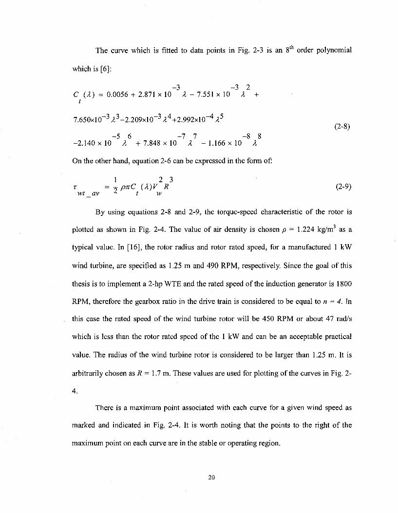
The curve which is fitted to data points in Fig. 2-3 is an 8 order polynomial
which is [6]:
-3 -3 2 C (X) = 0.0056 + 2.871 x 10 X - 7.551 x 10 X +
t
7.650xl0~3 ;i3-2.209x10~3 A4+2.992x10~4 X5
(2-8) c £ n n o o
-2.140x10 X +7.848x10 X -1 .166x10 X
On the other hand, equation 2-6 can be expressed in the form of:
1 2 3 T = T pnC (X)V R (2-9)
wt _av l t w
By using equations 2-8 and 2-9, the torque-speed characteristic of the rotor is
plotted as shown in Fig. 2-4. The value of air density is chosen p = 1.224 kg/m as a
typical value. In [16], the rotor radius and rotor rated speed, for a manufactured 1 kW
wind turbine, are specified as 1.25 m and 490 RPM, respectively. Since the goal of this
thesis is to implement a 2-hp WTE and the rated speed of the induction generator is 1800
RPM, therefore the gearbox ratio in the drive train is considered to be equal to n = 4. In
this case the rated speed of the wind turbine rotor will be 450 RPM or about 47 rad/s
which is less than the rotor rated speed of the 1 kW and can be an acceptable practical
value. The radius of the wind turbine rotor is considered to be larger than 1.25 m. It is
arbitrarily chosen as R = 1.7 m. These values are used for plotting of the curves in Fig. 2-
4.
There is a maximum point associated with each curve for a given wind speed as
marked and indicated in Fig. 2-4. It is worth noting that the points to the right of the
maximum point on each curve are in the stable or operating region.
20
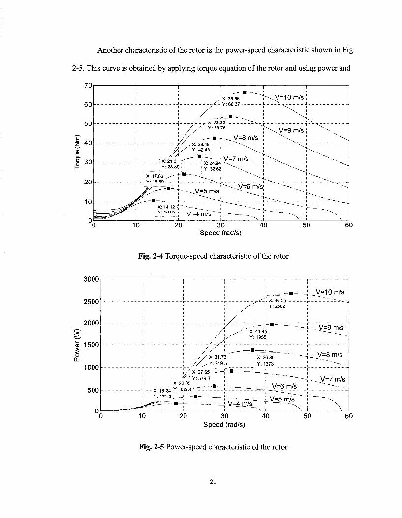
Another characteristic of the rotor is the power-speed characteristic shown in Fig.
2-5. This curve is obtained by applying torque equation of the rotor and using power and
30 Speed (rad/s)
Fig. 2-4 Torque-speed characteristic of the rotor
CD
o Q_
3000
2500
2000
1500
1000
500
30 Speed (rad/s)
Fig. 2-5 Power-speed characteristic of the rotor
21

torque relationship which isPwt=TwtO)wt. The power-speed characteristic of the rotor
shows that the converted power varies with the wind and shaft speeds. There is a
maximum output power for each wind speed, which occurs at different shaft speeds.
Besides, the maximum power increases as the wind speed increases. This reveals the fact
that for maximum power tracking with varying wind speeds, the wind turbine must
operate at variable speed. In other words, a control strategy must be applied in such a way
that by varying the load at the generator output, it enforces the wind turbine to operate at
the desired speed. By comparing Fig. 2-4 and Fig. 2-5 one can conclude that maximum
power does not correspond to the maximum torque. In other words, for a certain wind
speed, maximum power and maximum torque do not occur at the same rotor speed.
2.2.3 OSCILLATORY TORQUE
In reality the torque produced by the rotor is not constant, even though the wind
speed is considered to be constant. The most important facts which create some
pulsations on the produced torque are tower shadow and wind shear or gradient effects
[3].
For down-wind wind turbines, the tower shadow effect is significant since the
tower blocks the air flow. Thus, the wind speed behind the tower reduces significantly.
The tower shadow effect for the down-wind wind turbines is also called tower dam effect
in the literature. For up-wind wind turbines, the wind speed reduces in front of the tower.
This happens because of the fact that air flow will be disturbed by the tower and its speed
reduces comparing with the case when the air flow is undisturbed [3]. The effect of tower
22
shadow is highly reduced for the modern up-wind turbines by manufacturing slender
towers [3].
However, for both types of wind turbines, every time a blade passes in front of the
tower it faces lower wind speed comparing with the situations where the blade is in any
other position. Therefore, whenever a blade is in front of the tower, it produces lower
torque. The tower shadow effect on producing torque is shown in Fig. 2-6 as described
and investigated in [17] for a 3-bladed wind turbine. As it is shown, there are 3 pulse-like
torque reductions in one rotation of the rotor which can be considered as 3rd harmonic of
the rotor speed. It should be noted that the plots in Fig. 2-6 are just indicative (also not to
scale) and presented for better understanding of this discussion.
Wind shear or wind gradient effect is based on the fact that wind speed is higher
at higher altitude. Because of the friction of the moving air particles with ground the air
flow closer to ground will be slower than the air flow at higher altitude [3]. This means
that each blade faces different wind speeds as it rotates even when there is no wind speed
variations are considered. It is reported in [17] that the produced torque by each blade has
a sinusoidal form as shown in Fig. 2-6(a). It should be noted that Fig. 2-6(a) shows the
tower shadow effect and wind shear effect for each blade for one complete rotation of
each blade.
Fig. 2-6(b) shows the total torque produced by all 3 blades, considering that the
performances of the blades in producing torque are identical. In this case, as it is clear
from the Fig. 2-6(b), the wind shear has no effect because of the symmetry of the 3-blade
rotor [17]. But as it is discussed in [17], in practice, the performance of, for instance, one
blade might be lower than the others due to manufacturing inaccuracy or by deformation
23
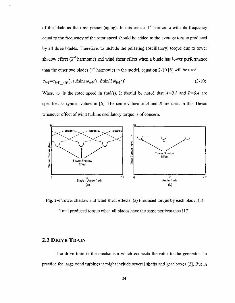
of the blade as the time passes (aging). In this case a 1st harmonic with its frequency
equal to the frequency of the rotor speed should be added to the average torque produced
by all three blades. Therefore, to include the pulsating (oscillatory) torque due to tower
shadow effect (3rd harmonic) and wind shear effect when a blade has lower performance
than the other two blades (1st harmonic) in the model, equation 2-10 [6] will be used.
Twt=*wt _av[l+Asia(a>wtt)+Bsm(3a)wtt)] (2-10)
Where cor is the rotor speed in (rad/s). It should be noted that A=0.2 and B=0,4 are
specified as typical values in [6]. The same values of A and B are used in this Thesis
whenever effect of wind turbine oscillatory torque is of concern.
Blade 1 Angle (rad)
(a)
n Angle (rad)
(b)
Fig. 2-6 Tower shadow and wind shear effects; (a) Produced torque by each blade; (b)
Total produced torque when all blades have the same performance [17]
2.3 DRIVE TRAIN
The drive train is the mechanism which connects the rotor to the generator. In
practice for large wind turbines it might include several shafts and gear boxes [3]. But in
24
this Thesis the drive train consists of two shafts and a gearbox, for two reasons. First, a
small WTE is proposed. Second, the concept can be developed for more complicated
drive trains. The shaft which connects the rotor to the gearbox (low speed side shaft) is
considered to be flexible and the shaft which connects the gearbox to the generator (high
speed side shaft) is considered to be rigid. These are acceptable assumptions since the
low speed side shaft is longer than high speed side shaft and the amount of torque on the
low speed side shaft is greater than the torque on the high speed side shaft by the factor of
gear ratio [18]. The gearbox is considered to be ideal.
The effect of the drive train on the system differential equations is taken into
consideration in section 2.4. The drive train can be simplified as a flexible shaft which is
connected to a mass on each side. These are all energy storage elements where masses
store energy in the form of kinetic energy due to their rotational speeds. The flexible shaft
stores the energy in the form potential energy due to its twist. Transferring energy from
the flexible shaft to each mass or vice versa will occur, whenever any of the inputs or
outputs of the system varies. The combination of masses moment of inertias and the
flexible shaft presents very low resistance to system inputs or outputs at certain
frequencies. These frequencies are called natural frequencies which depend on the values
of mass moment of inertias and the shaft torsional spring constant [19].
Thus, if any of the system's inputs or outputs presents a variation at or close to
any of the natural frequencies, one should expect a large amount of energy transfer from
one element to another. As it will be observed in the simulation results in this Chapter,
excitation of the natural frequencies results in variation on the torque on the high speed
side shaft. This might exceed the shaft and the generator capacities and result in
25

damaging the shaft or generator or both if it is not damped out. The flexible shaft
damping plays an important role in suppressing those variations.
Therefore, in this section the drive train natural frequencies are investigated.
Equations for calculating the shaft torsional spring constant and shaft damping constant
are also presented.
2.3.1 NATURAL FREQUENCIES
Fig. 2-7(a) depicts the rotor and hub which represent about 90% of the wind
turbine mass moment of inertia Jwt, on one side of the flexible shaft and the generator
with the mass moment of inertia Jgen, on the other side of the shaft [20]. It is assumed that
the masses moment of inertias of the shafts and the gear box in the drive train are lumped
into the rotor's and the generator's masses moment of inertias. The gearbox is omitted
from the drive train model in Fig. 2-7 by referring the generator mass moment of inertia
to the low speed side. To do that, the generator moment of inertia is multiplied by n2
where the gear ratio is assumed to be n:l [18]. The shaft torsional spring constant is Kst,-
In terms of system natural frequencies, the configuration in Fig. 2-7(a) has two degrees of
freedom [19].
One mode corresponds to the case where the rotor and the generator start to
oscillate around the flexible shaft if its modal natural frequency is excited. The other
mode corresponds to the case where the generator rotates at the fixed speed. This might
happen when the generator is connected to a strong grid, in this case, only the rotor starts
to oscillate around the shaft if its modal natural frequency is excited. Fig. 2-7(b) indicates
the equivalent model for the latter case just for the purpose of calculating the system
26
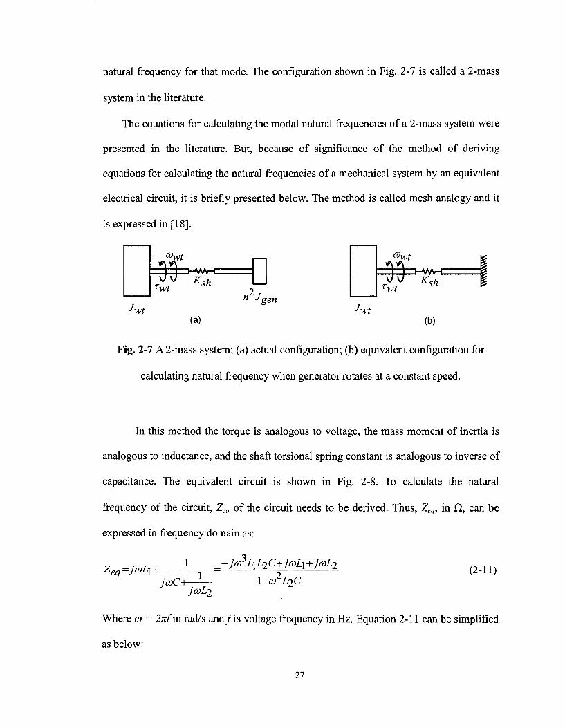
natural frequency for that mode. The configuration shown in Fig. 2-7 is called a 2-mass
system in the literature.
The equations for calculating the modal natural frequencies of a 2-mass system were
presented in the literature. But, because of significance of the method of deriving
equations for calculating the natural frequencies of a mechanical system by an equivalent
electrical circuit, it is briefly presented below. The method is called mesh analogy and it
is expressed in [18].
<°wt
J-wt
IHWlr-C Ksh
(a)
n2J gen
°>wt
Twt
J wt
ZHVW-C Ksh
(b)
Fig. 2-7 A 2-mass system; (a) actual configuration; (b) equivalent configuration for
calculating natural frequency when generator rotates at a constant speed.
In this method the torque is analogous to voltage, the mass moment of inertia is
analogous to inductance, and the shaft torsional spring constant is analogous to inverse of
capacitance. The equivalent circuit is shown in Fig. 2-8. To calculate the natural
frequency of the circuit, Zeq of the circuit needs to be derived. Thus, Zeq, in Q, can be
expressed in frequency domain as:
1 Zeq=J<»L\-
jcoC+- 1 J<oLi
3 -jco L\L2C+jcoL\+jo)L2
\-co2LjC (2-11)
Where a> = 2xf in rad/s and/is voltage frequency in Hz. Equation 2-11 can be simplified
as below:
27

6 =^C
-eq
Fig. 2-8 Mesh analogy of Fig. 2-7(a)
_ja)(Li+L2-cozLiL2C)
l-o)ZL2C (2-12)
By equating the numerator of equation 2-12 to zero, the natural frequency of the circuit,
in Hz, is:
f -_L ILL _L̂ Jn~2^C^Ll
+L2)
(2-13)
Now, by referring to definition of mesh analogy and replace Lj, L2, and C by Jwt, n2Jge„,
and 1/Ksh, respectively, one of the natural frequencies of the 2-mass system, in Hz, will
be:
/ , 1 \r < l l ^ (2-14)
'wt n J, gen
The other natural frequency of the 2-mass system, in Hz, can be obtained by removing L2
from the circuit in Fig. 2-7 and setting the term l/n2Jgen in equation 2-14 equal to zero.
Thus, it will be:
/ , 1 \Ksh
"2 2n\J, (2-15)
wt
28

Therefore, these frequencies should not be excited to avoid resonance effect
during operation of wind turbines. It is also suggested, in the literature, to introduce
additional damping (by special design) to suppress the amplitude of torque whenever the
system's natural frequencies are excited.
2.3.2 SHAFT TORSIONAL SPRING AND DAMPING CONSTANTS
The following equations [19] are used for calculating torsional spring constant
(Ksh) of a shaft with the dimensions which are shown in Fig. 2-9. Angle 6sh is the shaft
twist in rad.
Fig. 2-9 Shaft with length /,/, and radius rs% [19]
4 nr 7 Sri
Jsh=-^- (2-16)
Where Jsh is the shaft polar moment of inertia in m4 and rSh is the shaft radius in m. Thus,
Ksh in Nm/rad can be expressed as:
Ksh=^ (2-17)
lsh
Where G is the shear modulus of the material in N/m2rad and / is the shaft length in m.
The flexible shaft damping constant can be generally calculated based on equation
2-18 which is related to a 2-mass system of Fig. 2-7(a) [21]:
29

Bsh=^sh t K s \ (2-18)
ywt n2Jgen
Where BSh is the shaft damping constant in Nms/rad, ^represents the damping ratio. It
is experimentally determined to be in the range of 0.005 to 0.075 [21]. The damping ratio
(<^sh) is 0.0175 for steel material [22]. This value will be used for calculating of shaft
damping throughout this Thesis. Equation 2-18 reveals that the shaft damping constant
not only depends on the material of the shaft but also on the shaft torsional spring
constant and the masses moment of inertias on both sides.
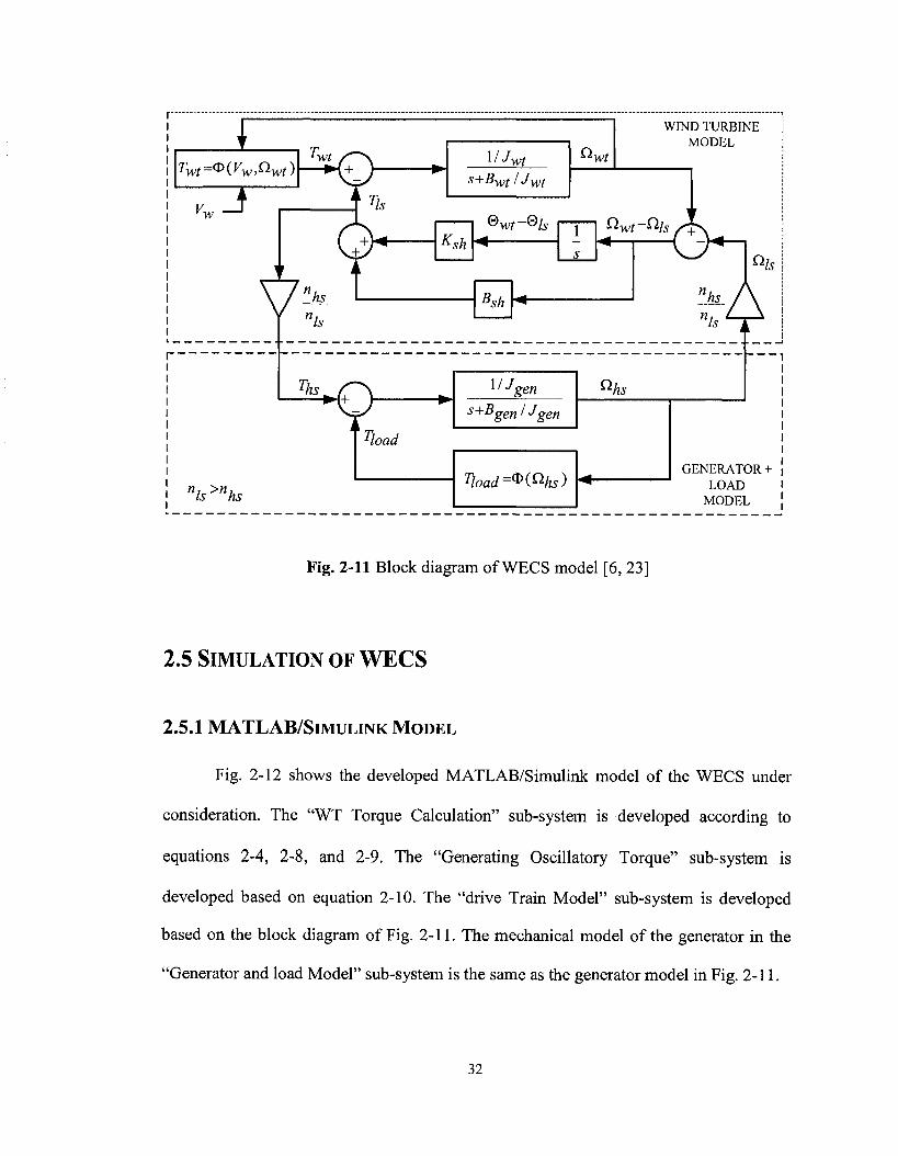
2.4 WECS DIFFERENTIAL EQUATIONS AND BLOCK DIAGRAM
The WECS model is shown in Fig. 2-10. The model includes a wind turbine with
the mass moment of inertia (Jwt) and friction damping (Bwt), low speed side shaft with the
torsional spring constant (KSh) and damping (Bsf,), gear ratio (n&/«fo), a rigid high speed
side shaft, and electrical generator with the mass moment of inertia (Jgen) and friction
damping (Bgen). The differential equations which describe the presented model are
expressed in the following equations [6, 23].
d26wt d6wt dOwt dOis J = T - jj B ( y
ai (2-19)
- K (& - 9 ) sh wt Is
30

J\vt
TWtO
30
5 B wt
K
sh
GEARBOX
\n Is
J gen
wm Ths@hs
3 Tload
B, gen
Fig. 2-10 WECS model [6]
Equation 2-19 is the differential equation which can be applied to the low speed side
shaft. It includes the rotor, hub and the flexible shaft. The differential equation which
represents the high speed side shaft is as follows:
Jgen 2 dt7 — Ths "gen , Tload (2-20)
The relationship between torques and positions on both sides of the gearbox are:
% _ % -n
Ths nhs
6ls=nhsJ
Qhs nls n (2-21)
Considering the above mentioned equations, the block diagram of the model of
Fig. 2-10 is built as indicated in Fig. 2-11, which shows that xwt is a function of Vw and
coWf It also shows that the load is a function of wind turbine rotor speed. The load
function is defined in section 2.5.1.
31
T V,
nls>nhs
\Hoad
\IJ-wt S+Bwt/J\vt
Ksh ®wt~®ls
Bsh
\IJ gen
Q. wt
s+Bgen/Jgen
Tload=®(&hs)
WIND TURBINE MODEL
n, i , \
&hs
GENERATOR + LOAD
MODEL
Fig. 2-11 Block diagram of WECS model [6, 23]
2.5 SIMULATION OF WECS
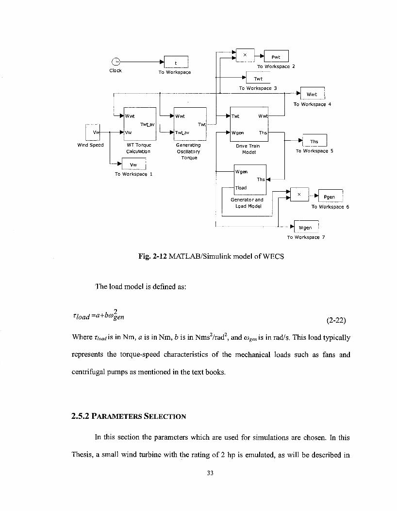
2.5.1 MATLAB/SIMULINK MODEL
Fig. 2-12 shows the developed MATLAB/Simulink model of the WECS under
consideration. The "WT Torque Calculation" sub-system is developed according to
equations 2-4, 2-8, and 2-9. The "Generating Oscillatory Torque" sub-system is
developed based on equation 2-10. The "drive Train Model" sub-system is developed
based on the block diagram of Fig. 2-11. The mechanical model of the generator in the
"Generator and load Model" sub-system is the same as the generator model in Fig. 2-11.
32
Wind Speed
To Workspace 6
To Workspace 7
Fig. 2-12 MATLAB/Simulink model of WECS
The load model is defined as:
rload =a+b(ogen (2-22)
Where z w i s in Nm, a is in Nm, b is in Nms2/rad2, and cogen is in rad/s. This load typically
represents the torque-speed characteristics of the mechanical loads such as fans and
centrifugal pumps as mentioned in the text books.
2.5.2 PARAMETERS SELECTION
In this section the parameters which are used for simulations are chosen. In this
Thesis, a small wind turbine with the rating of 2 hp is emulated, as will be described in
33
Chapters 3 and 4. Because of lack of enough information for small wind turbines some
parameters are selected arbitrarily. The wind turbine rotor radius, R = 1.7 m, and gear
box ratio, n - 4, are selected as discussed in section 2.2.2. The wind turbine mass
moment of inertia and friction coefficient are considered to be Jwt = 3 kgm , and Bwt =
0.1 Nms/rad, respectively. A procedure of calculating the wind speed at which the wind
turbine produces 2 hp on the generator shaft, for the selected wind turbine parameters, is
provided in Appendix A.
The generator mass moment of inertia and friction coefficient are considered as
Jgen = 0.0203 kgm2 and Bgen = 0.003075 Nms/rad, respectively. These values are
estimated values of total masses moment of inertias of two PMDC machines (one as
prime mover and the other one as dynamometer) used as wind turbine emulator discussed
in Chapter 3. In this case, it will be easier to compare the simulation results in this
chapter and experimental results which will be presented in Chapter 3.
Based on equation 2-22, the load coefficient is defined as a = 0 Nm and b -
182xl0"6 Nms2/rad2. It should be noted that the load coefficient will be changed for
different case studies.
Referring to equations 2-16 and 2-17, with rsh = 0.009 m and lsh = 0.5 m, and
assuming that the shaft is made of steel with shear modulus G = 83*l(f Pa, shaft
torsional constant can be calculated as Ksh =1710.80 Nm/rad.
According to equation 2-18, the shaft damping constant can be calculated as BSh =
0.7837 Nms/rad.
34
2.5.3 SIMULATION RESULTS
Simulation results are provided for six different cases which include the steady-
state and transient responses. The parameters for the simulation results are the same as
parameters provided in Table 2-1, unless otherwise stated.
Table 2-1 Parameters used for simulation results
Wind Turbine, Generator, and Mechanical Load Parameters
Wind Turbine
Jwt (kgm2) 3
Bwt (Nms/rad) 0.1
Ksh (Nm/rad) 1710.8
Bsh (Nms/rad) 0.7837 n 4
Generator and Mechanical Load Constants
Jgen (kgm2) 0.0203
Bgen (Nms/rad) 0.0030725
a (Nm) 0
b (Nms2/rad2) 0.000182
Case 1) This case highlights the effect of the wind turbine mass moment of inertia
on filtering of the oscillatory torque as far as generator torque and speed are concerned.
The results for this case are shown in Fig. 2-13. The results are taken in steady-state. The
wind speed is constant at Vw = 8.25 m/s. The responses are shown for wind turbines with
mass moment of inertia (Jwt) equal to 1 and 10 kgm2. According to equation 2-18, the
shaft damping (Bsh) are 0.7168 and 0.8120 Nms/rad, respectively.
The results show that for the wind turbine with higher mass moment of inertia the
variations on the wind turbine rotor speed, high speed side torque (generator shaft), and
generator speed are lower than the wind turbine with lower mass moment of inertia.
Higher mass moment of inertia can be achieved by fabricating larger and heavier blades
35
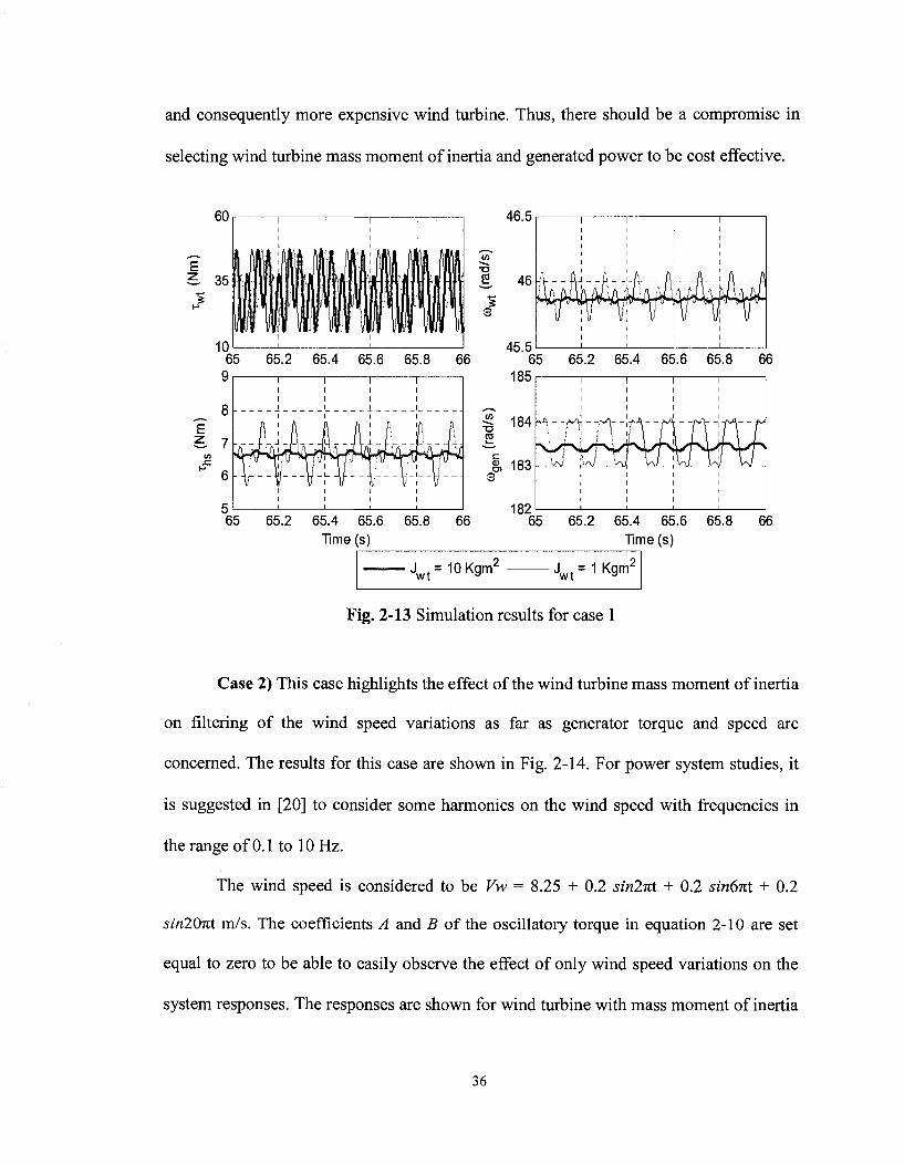
and consequently more expensive wind turbine. Thus, there should be a compromise in
selecting wind turbine mass moment of inertia and generated power to be cost effective.
9
_ 8 i" 5. 7
1 1 1 1
1 i 1 1
J l ' f t 11 f l ' IS ' 1 i l
i [ W i | j i j J
1 1 1 1
^ 184
g, 183
65 65.2 65.4 65.6 65.8 66 182
— ~ v -_>, .--w ^ ~ _ .* ̂ ^ --tf . *, - _
Time s) 65 65.2 65.4 65.6 65.8
Time (s)
J =10Kgm^ wt uwt
1 Kgm"
Fig. 2-13 Simulation results for case 1
66
Case 2) This case highlights the effect of the wind turbine mass moment of inertia
on filtering of the wind speed variations as far as generator torque and speed are
concerned. The results for this case are shown in Fig. 2-14. For power system studies, it
is suggested in [20] to consider some harmonics on the wind speed with frequencies in
the range of 0.1 to 10 Hz.
The wind speed is considered to be Vw = 8.25 + 0.2 sin2iti + 0.2 sin6izt + 0.2
sm207rt m/s. The coefficients A and B of the oscillatory torque in equation 2-10 are set
equal to zero to be able to easily observe the effect of only wind speed variations on the
system responses. The responses are shown for wind turbine with mass moment of inertia
36
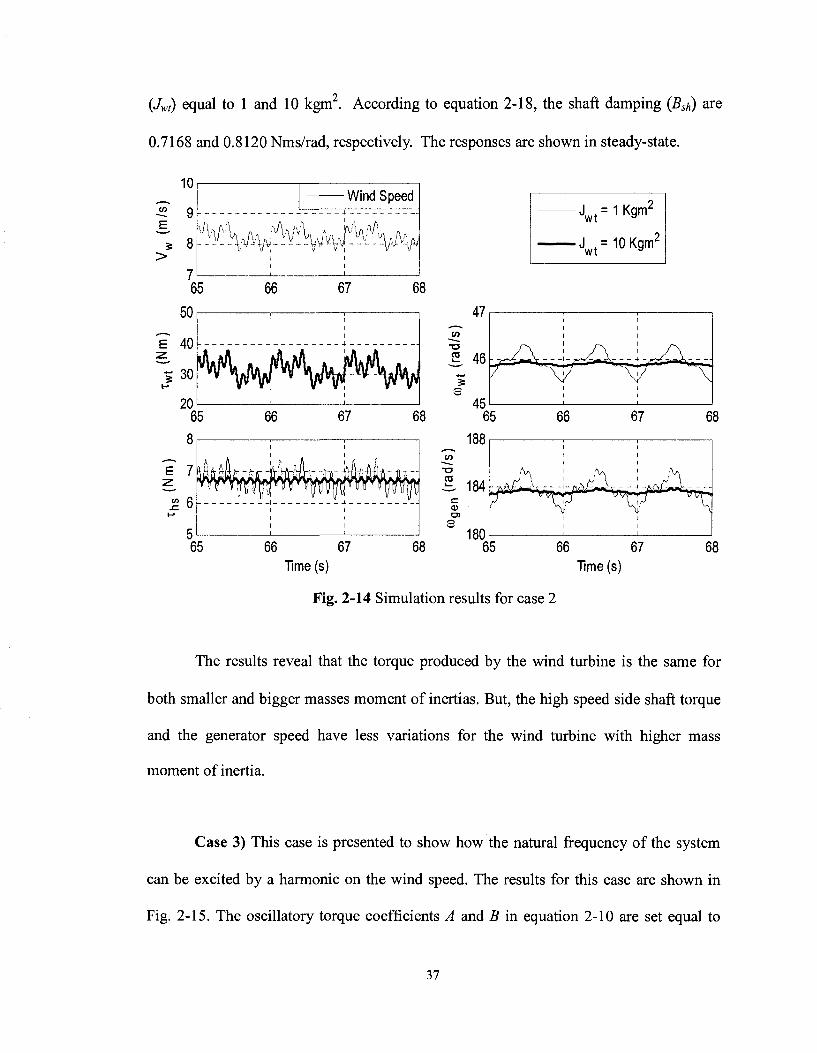
(Jwt) equal to 1 and 10 kgm2. According to equation 2-18, the shaft damping (BSh) are
0.7168 and 0.8120 Nms/rad, respectively. The responses are shown in steady-state.
10
i» 9 E UV\ iV%
Wind Speed
A J V ^ V ^ 65 66 67 68
66 67 Time (s)
66 67 Time (s)
Fig. 2-14 Simulation results for case 2
The results reveal that the torque produced by the wind turbine is the same for
both smaller and bigger masses moment of inertias. But, the high speed side shaft torque
and the generator speed have less variations for the wind turbine with higher mass
moment of inertia.
Case 3) This case is presented to show how the natural frequency of the system
can be excited by a harmonic on the wind speed. The results for this case are shown in
Fig. 2-15. The oscillatory torque coefficients A and B in equation 2-10 are set equal to
37

zero. Therefore, the variations on the system responses are due to only wind speed
harmonics. Two wind speed profiles are considered for the system with the same
parameters. They are Vw = 8.25 + 0.4 sin6nt m/s and Vw = 8.25 + 0.4 sinlAiti. m/s. The
responses are presented in steady-state.
10
9
8 '^jv^Ah/crKf. 25
40 r
35 I I
30
25
10
8
6
25.2 25.4 25.6 25.8
25 25.2 25.4 25.6 25.8
25 25.2 25.4 25.6
Time (s)
£
E 1
•S 0.5
26
- r m n rrr T r n -r«- T rrr T r - n r r
46.5
46
26 45.5
25
i M f'l J \ / I' f 1 / \ V I f l M / I I t "1 If 1 |[4"4-"> lMlT"".' \ j bl.„L,.U.jl «T""J fl IllnlnJ L
25.8 26
1 L
X:3 Y: 0.09683
•
. 1 ; X: 12 i Y: 1.128
1 1
5 10
Frequency (Hz) 15
F^^Z^Si^.y^y^^Sir^~^^
25.2 25.4 25.6 25.8 26
25.2 25.4 25.6 25.8
Time (s) 26
. Results related to V with 3 Hz Variations Results related to V,, with 12 Hz Variations W
Fig. 2-15 Simulation results for case 3
As it can be seen from the results, the variations on the high speed side shaft
torque for the wind speed with 12 Hz variations is significantly larger than when wind
has a 3 Hz component. The reason is that, 12 Hz is very close to the system's natural
frequency which is, according to equation 2-14, 12.16 Hz. Thus, larger variations should
be expected on the output responses when the wind speed presents variations at
frequencies closer to the system's natural frequency. It should be noted that the FFT of
the high speed side shaft torque shows the 3 and 12 Hz components which correspond to
38
3 and 12 Hz variations on the wind speed. It can be also seen that the wind turbine speed
variation for the wind speed with 3 Hz component is larger than the case where it has 12
Hz component. It is because of the fact that the torque with the lower frequency results in
a larger variation on a mass with inertia.
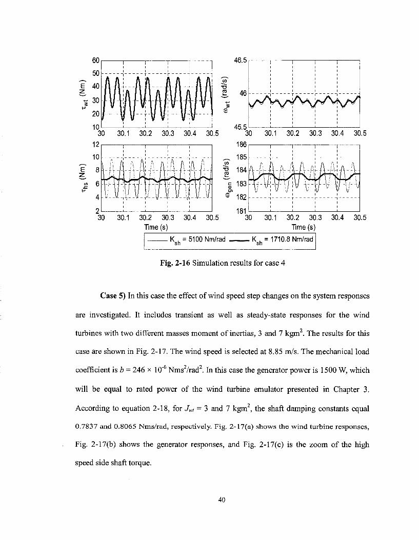
Case 4) This case shows how oscillatory torque can excite the natural frequency
of the system. The results for this case are shown in Fig. 2-16, in steady-state. The
oscillatory torque is in effect. The wind speed is constant at 8.25 m/s. Therefore, the
variations on the system responses are due to the oscillatory torque only. Systems with
two different shaft torsional spring constants (KSh), 5100 and 1710.8 Nm/rad are
considered. It should be noted that according to equation 2-18, the shaft damping
constants (Bsh) are 1.35 and 0.7837 Nms/rad, respectively.
Referring to Fig. 2-16, it can be clearly seen that the variations on the high speed
side shaft torque is much larger in the case where Ksu is 5100 Nm/rad. The reason is that
the natural frequencies of the system, based on equation 2-14, with KSh = 5100 Nm/s and
KSh = 1710.8 Nm/s are 20.99 and 12.16 Hz, respectively. On the other hand, the 3rd
harmonic of the wind turbine rotor speed is equal to 21.875 Hz. Since, this frequency (3rd
harmonic) is much closer to the natural frequency of the system with Ksh = 5100 Nm/s,
larger variations should be expected for the case where KSh = 5100 Nm/s comparing to the
case where Ksh = 1710.8 Nm/s.
39
60
50
40
? 30
20
10
1 I I I
1 T
I I I L i i i J l i . I ii I J 1 i u^ i i 'i 11 J 1 1 1 1 '
—
H-l
i
i '
- — i -
"""l W
5>
j - f l
46.5
12
10
E* 8
m 6
4
T3 "3
5 s
30 30.1 30.2 30.3 30.4 30.5
! r ( . I A A1 A N ' A A ' i \ A ' l\ A 1 ) I l l / I [ V J 1 l l ' l l J \ ' I 1 I I / T F T ~\\~ 7 T " H + 1 r f l t-J—[— 4 j - H H - i 4 - I
i Li r' f \ Li' I I I' O I i '] 1 LA I
_ U _ -\L -,-lJ- - U - Tv- - y _ _\L - -U- - l / i - -V- - U _
45.5
186
30.5
_̂_̂ 0)
T 3 TO
c (U O)
3
185
184
183
ia?
30 30.1 30.2 30.3 Time (s)
30.4 30.5 181
( T ( ! ft f\ A A ' A A ' A
A J 1 r ! A i\ r i A ' / \ f \ ' A r l
_ T ] „ V L' _i_/_ r 11 U_ 1 j _ r L A J _ 1' i _irj_ 4 j
""17 v 1 I / "l f 1 v "17 f / v 1' f 1 / v
1 T 1 1
30 30.1 30.2 30.3 Time (s)
30.4 30.5
K = 5100Nm/rad sh
K . = 1710.8 Nm/rad sh
Fig. 2-16 Simulation results for case 4
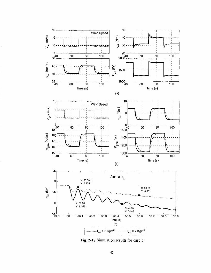
Case 5) In this case the effect of wind speed step changes on the system responses
are investigated. It includes transient as well as steady-state responses for the wind
turbines with two different masses moment of inertias, 3 and 7 kgm2. The results for this
case are shown in Fig. 2-17. The wind speed is selected at 8.85 m/s. The mechanical load
coefficient is b = 246 x 10"6 Nms2/rad2. In this case the generator power is 1500 W, which
will be equal to rated power of the wind turbine emulator presented in Chapter 3.
According to equation 2-18, for Jwt = 3 and 7 kgm2, the shaft damping constants equal
0.7837 and 0.8065 Nms/rad, respectively. Fig. 2-17(a) shows the wind turbine responses,
Fig. 2-17(b) shows the generator responses, and Fig. 2-17(c) is the zoom of the high
speed side shaft torque.
40

The results show that the transient response for wind turbine with higher mass
moment of inertia is slower. Another point is that the wind speed change causes
overshoot or undershoot on the wind turbine torque and power responses but the other
responses such as wind turbine rotor speed and the high speed side responses are under-
damped.
The other fact is that every time the wind speed changes, the system's mechanical
mode will be excited. This fact is shown in Fig. 2-17(c). The natural frequencies of the
system for Jwt equal to 3 and 7 kgm2, according to equation 2-23, are 12.16 and 11.81 Hz,
respectively. According to Fig. 2-17(c), the calculated values of natural frequencies for
the wind turbine with the masses moment of inertias of 3 and 7 kgm are 12.19 and 11.76
Hz, respectively. The small differences are because of the accuracy of simulation results,
since they have been executed with fixed step sampling time. It should be noted that the
condition for exciting the natural frequency, introduced by equation 2-15 as discussed in
section 2.3.1, is to somehow keep the generator speed constant. Since this condition
cannot be provided unless the generator is connected to a strong grid (regulated system),
the excitation of this mode does not occur.
41
10
9
8
50
45
40
,40
35 40
10
9.5
1*1 . J c ,
J L
60 80 100
r 60 80
Time (s) 100
I
J
- Wind Speed
, I 1
60 80 Time (s)
50
E" 40
5 30
20
Y^
k
2000
1500
,40 60 80
1000 40 60 80
Time (s)
(a)
(b)
60 80 Time (s)
100
i i i
i i . i
i t i
i i t
100
8.5
7.5 I— 49.9
Zoom of-X: 50.08 Y: 8.724
to
X: 50.59 Y: 8.351
Y: 8.158 X: 50.45 Y: 7.945
50 50.1 50.2 50.3 50.4 50.5 50.6 50.7 Time (s)
(c)
50.8
' J w t = 3 K g m 2 J w ( = 7 Kgm2
50.9
Fig. 2-17 Simulation results for case 5
42
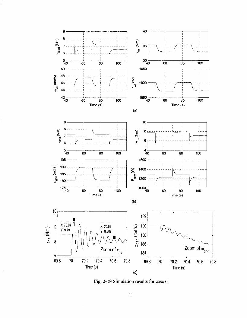
Case 6) This case is intended to investigate the effect of load step changes on the
system responses. It includes transient as well as steady-state responses. The results are
shown in Fig. 2-18. The wind speed is selected at 8.5 m/s. The mechanical load
coefficient is b = 220 x 10"6 Nms2/rad2. In this case the generator power is about 1300 W.
These values are chosen since the wind turbine emulator in Chapter 3 will be tested with
the same values for ease of comparison. Selecting these values allow the following load
step changes with slightly exceeding the rated speed and torque of the prime mover in
ft 9 9
experimental set-up of Chapter 3. The load step changes are ± 40 x 10" Nms /rad . Fig.
2-18(a) shows the wind turbine responses and Fig. 2-18(b) shows the generator
responses. Fig. 2-18(c) is the zoom of the high speed side shaft torque and the generator
speed.
The importance of the load change, as it can be seen from the results, is the
excitation of the system's mechanical mode. Referring to equation 2-14, the natural
frequency of the system is 12.16 Hz. According to the points highlighted in Fig. 2-18(c)
the calculated natural frequency is 12.12 Hz. The slight difference is for the same reason
as discussed in the end of previous case. The other point is that the responses on the wind
turbine side are all over-damped. On the other hand, the load changes result in overshoot
and undershoot on the generator torque and power responses.
43
E z I ft, I 1 Pv L H \ t-
_i i.
40
<n
2
50
48
46
44
42 40
60 80
60 80 Time (s)
100
100
40
Z 35
30
H f- 1
40 1650
60 80
1600 k—-^ H
1550 60 80
Time (s)
100
9
? 8 £ 7
CO
^ 6
I I I I I i
— _,—
Y-\—
K \ ; — j . —
Y—\— i
40
195
S 190
g. 185
180
175 40
60 80
60 80 Time (s)
100
100
10
8
6
40
1600
1400
1200
1000 40
(b)
60 80
60 80 Time (s)
r 100
— I I l^-r-1 J
100
(c)
70.2 70.4 Time (s)
Fig. 2-18 Simulation results for case 6
44

2.6 CONCLUSIONS
This chapter has focused on the modeling of WECSs. In doing this, the power
coefficient, and torque coefficient were introduced. Consequently, the power and torque
equations were expressed and the torque-speed and power-speed characteristics of a
typical wind turbine based on the given C(X) curve were presented. The drive train with a
flexible shaft and gearbox were discussed and the equations for calculating natural
frequencies of a 2-mass system with 2 degrees of freedom were given. The system under
consideration was presented in Fig. 2-9 which mainly includes the mechanical model of
the wind turbine, the electric generator, and the load. The wind turbine rotor was simply
modeled as a mass moment of inertia and friction damping mainly due to the blades and
the hub.
The wind turbine drive train was considered as a shaft, which was modeled with its
torsional spring constant and damping constant, and an ideal (lossless and backlash free)
gearbox. The electric generator was modeled with its mass moment of inertia and friction
damping. An expression between load torque and speed of generator was assigned as a
load model. After expressing the differential equations governing the system, the
developed block diagram was presented in Fig. 2-10. Based on the block diagram and
other equations the system was modeled in MATLAB/Simulink. The simulation results
were presented and some important facts as summarized below were observed.
> Effect of the wind turbines with higher mass moment of inertia in filtering
the wind speed variations and pulsations due to oscillatory torque on the
generator torque.
45

> System resonance occurrence due to wind speed variations, load variations,
and also due to oscillatory torque.
> Slower transient response for the system with higher wind turbine mass
moment of inertia.

CHAPTER 3
DESIGN AND IMPLEMENTATION OF A WTE
3.1 INTRODUCTION
The mechanical parts of a wind turbine, including the rotor and the drive train,
were modeled and discussed in Chapter 2, as the first step. The second step is to design
and implement a system to follow the reference torque at the high speed side shaft, as if
driven by the wind turbine. The system includes a prime mover, power electronics
converter, and a controller in addition to the wind turbine model. The wind turbine model
generates the reference torque and communicates with the system through a real-time
software.
As it was discussed in Chapter 1, after reviewing the literature a PMDC machine
is chosen as prime mover. In this case, by knowing the relationship between torque and
current of the DC machine, it is possible to enforce the machine to produce the desired
torque by controlling its current. A switch-mode DC-DC converter and a hysteresis
current controller are chosen to enforce the prime mover to follow the reference torque on
its shaft. It should be noted that the prime mover will run a PMDC machine as
dynamometer, which behaves as a mechanical load. In this case without having a
generator and variable electrical load, it is possible to make the system operate at
different operating points (torque vs. speed characteristic of the wind turbine) by
controlling the torque of the dynamometer.
Section 3.2 describes the PMDC machines and their characteristics. In section 3.3
the power electronics and type of controllers are discussed. Section 3.4 is devoted to
47
describing the logic of the WTE. The experimental set-up and the methods of
implementation of the WTE are discussed in section 3.5. The experimental results are
provided in section 3.6 and section 3.7 summarizes this Chapter and provides the
conclusions.
3.2 PMDC MACHINES
DC machines have been used in motor drives since long time. They have very
good drive performance which makes them relatively easy to control to follow the
reference speed and/or torque. The main disadvantage of DC machines was very high
maintenance requirement for brushes and commutators. Development in brushes and
commutator technologies made it possible to design them with longer life time and lower
maintenance requirement. With the advancement in rare-earth magnet, the PMDC
machines are designed with very high torque-to-volume and reasonable prices. Recently,
with the advancement in power electronics, the squirrel cage induction machines which
have low cost and rugged construction are used in motor drives [24,25].
There are different schemes to control the induction motor. Vector-controlled
schemes are among them which were proposed by researchers. They require more
complicated control strategies in comparison with DC machines due to their torque-speed
characteristics and AC quantities. Besides, their performances in motor drive applications
highly depend on the machine modeling and parameters. In this Thesis, because of the
availability of DC machines and power electronics switches suitable for DC machines in
the P. D. Ziogas Laboratory, and also the fact that, it is easier to control DC motors
compared to induction motors, a PMDC machine is used as prime mover.
48

3.2.1 M O D E L AND CHARACTERISTICS [24,25]
Based on the fact that PMDC machines produce constant flux as field, the
relationship between machine variables and parameters are as follows:
rem(t)=Ktia(t) (3-1)
Where xem is the electromechanical torque of the machine in Nm, Kt is the toque constant
of the machine in Nm/A, and ia is the machine's armature current in A.
eh{t)=Kb0im{t) (3-2)
Where e\> is back emf of the machine in V, Kb is the speed constant of the machine in
Vs/rad, and com is the machine speed in rad/s. It should be noted that in the SI unit system
the values of Kt and Kb are equal. By applying KVL to Fig. 3-1, which is the equivalent
circuit of the DC machine in motoring operation, the following equation can be written:
®m Tload
Fig. 3-1 PMDC machine equivalent circuit in motoring operation
^ ^ = ±v(t) - 3flLia(0 - JLe ( 0 (3.3) dt La La
aK) La bK)
Where vt is the terminal voltage in V, La is the armature inductance in H, and Ra is
armature resistance in CI. Furthermore, the torque and speed of the machine can be
related by the following equation:
d ^ L - ~^em (0 " -y-rioad (0 - ^ m (t) (3-4) at Jm Jm Jm
49

Where Jm is the mass moment of inertia of the machine in kgm2 and Bm is the machine
friction coefficient in Nms/rad. Considering equations 3-1 to 3-4 the following equation
expresses the DC motor in the form of state variables:
'dig(t) dt
dcom{t) . dt
Based on the above equations the DC motor model (block diagram in s domain) is shown
in Fig. 3-2.
Tfoad
1 I sJm +Bm
Fig. 3-2 PMDC motor model [25]
Fig. 3-3 shows the characteristics of PMDC machine. Fig. 3-3(a) shows the
relation between terminal voltage and machine speed where the torque or equivalently
armature current is kept constant at its rated value. In this case, the machine speed varies
linearly with varying terminal voltage. Therefore, at rated terminal voltage the machine
reaches the rated speed. The difference between vt and eb corresponds to iaRa voltage
drop. In Fig. 3-3(b) the relation between the torque and speed of the machines is
presented for individual terminal voltages. The characteristic implies that for a given
terminal voltage the machine can operate from zero to rated torque. One can see that for a
given terminal voltage the speed variation is limited to a very small range. As a result of
50
R,
Kt
Kb_
J m m m
ia(0
l(°m (Oj +
1 La
0 Vf(0 +
0 1
_ Jjn _
Tload (3-5)
0̂ sLa+Ra Kt
sm o-

these characteristics, it can be concluded that the machine can operate at any point in the
safe region (operating region) as marked ABCD, by controlling the terminal voltage and
machine torque. This characteristic provides the opportunity to use a DC machine as
prime mover for implementing WTE.
per unit T
quantities em
1.0
1 0 (per unit) Rated Speed
(a) (b)
Fig. 3-3 PMDC machine characteristics; (a) Continuous torque-speed capability; (b)
torque-speed characteristics for different terminal voltages where vt4 > v# > Vt2 > va [24].
3.2.2 PMDC MACHINE PARAMETERS
The PMDC machine parameters, including nameplate data, information from data
sheet, and estimated parameters, are provided in Table 3-1. The most important
parameter of the PMDC machine in implementing WTE is the torque constant Kt. This
parameter is estimated based on the method presented in [26] which is briefly described
below. The PMDC under test has been driven by another motor, operating as generator at
no-load. The generator voltages and speeds were measured and recorded. Therefore,
according to equation 2-2 the speed constant (Kb) was calculated. As stated earlier in this
chapter in the SI unit system, Kt = Kb.
51
Rated Torque
I 1 1
t: i
if ^COi ' K M
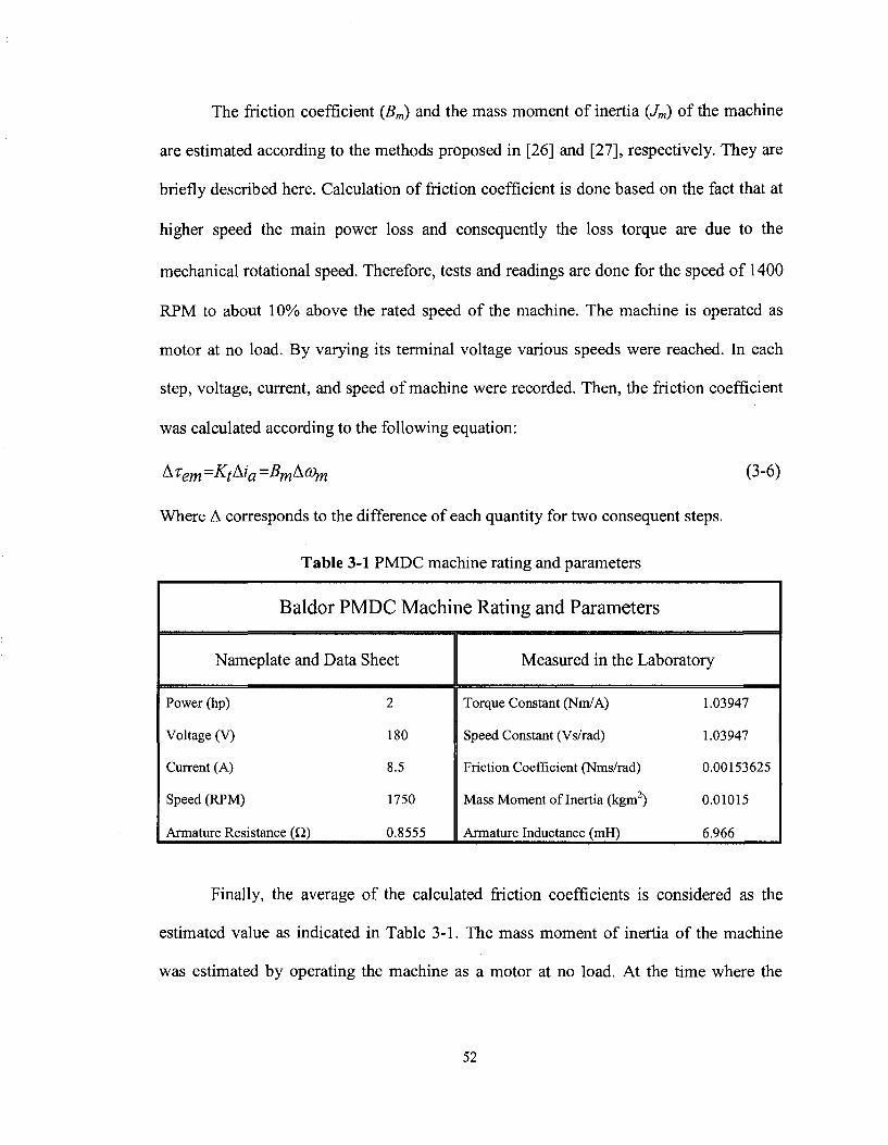
The friction coefficient (Bm) and the mass moment of inertia (Jm) of the machine
are estimated according to the methods proposed in [26] and [27], respectively. They are
briefly described here. Calculation of friction coefficient is done based on the fact that at
higher speed the main power loss and consequently the loss torque are due to the
mechanical rotational speed. Therefore, tests and readings are done for the speed of 1400
RPM to about 10% above the rated speed of the machine. The machine is operated as
motor at no load. By varying its terminal voltage various speeds were reached. In each
step, voltage, current, and speed of machine were recorded. Then, the friction coefficient
was calculated according to the following equation:
ATem=KtMa=Bm^(Om (3-6)
Where A corresponds to the difference of each quantity for two consequent steps.
Table 3-1 PMDC machine rating and parameters
Baldor PMDC Machine Rating and Parameters
Nameplate and Data Sheet
Power (hp) 2
Voltage (V) 180
Current (A) 8.5
Speed (RPM) 1750
Armature Resistance (£2) 0.8555
Measured in the Laboratory
Torque Constant (Nm/A) 1.03947
Speed Constant (Vs/rad) 1.03 947
Friction Coefficient (Nms/rad) 0.00153625
Mass Moment of Inertia (kgm2) 0.01015
Armature Inductance (mH) 6.966
Finally, the average of the calculated friction coefficients is considered as the
estimated value as indicated in Table 3-1. The mass moment of inertia of the machine
was estimated by operating the machine as a motor at no load. At the time where the
52

speed was about 1900 RPM, its breaker was opened. In this case, by referring to equation
3-4 and setting xem and T\oad to zero the solution of the differential equation is:
-Bm(t\-t0)
a>(t\)=co(t0)e Jm (3-7)
Since the speed versus time was plotted during the test, speeds at the time ti and t0
are known and the only unknown in equation 3-7 is Jm which was calculated as 0.009747
kgm2. This was the estimation of the mass moment of inertia of the PMDC machines by
the method explained above. But, the WTE itself also provided the opportunity to
estimate the mass moment of inertia of the PMDC machines which is briefly discussed in
section 3.5.4. The estimated value of mass moment of inertia of the PMDC machine by
using WTE was 0.01015 kgm2; this value is used as the estimation of each PMDC
machine mass moment of inertia.
3.3 POWER ELECTRONICS AND CONTROLLERS
To control the torque and speed of a DC machine, the average quantities such as
average armature current and terminal voltage are of concern. This can be done by line-
frequency controlled converters or switch-mode DC-DC converters. These concepts and
types of controllers involved are briefly described below.
3.3.1 L I N E - F R E Q U E N C Y CONTROLLED CONVERTERS [24]
These types of converters consist of thyristors which can be configured to work in
single-phase or three-phase systems. In Fig. 3-4 only single-phase configurations are
shown. In both configurations by creating proper firing angles for each thyristor the
53
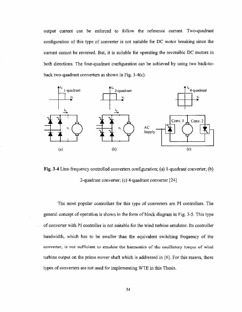
output current can be enforced to follow the reference current. Two-quadrant
configuration of this type of converter is not suitable for DC motor breaking since the
current cannot be reversed. But, it is suitable for operating the reversible DC motors in
both directions. The four-quadrant configuration can be achieved by using two back-to-
back two-quadrant converters as shown in Fig. 3-4(c).
* h 1-quadrant
• * '
(a)
2-quadrant
-£
(b)
AC . Supply
+ la 4-quadrant
3!
Conv. 1 1 Conv. 2
* o T
t (c)
Fig. 3-4 Line-frequency controlled converters configuration; (a) 1-quadrant converter; (b)
2-quadrant converter; (c) 4-quadrant converter [24]
The most popular controllers for this type of converters are PI controllers. The
general concept of operation is shown in the form of block diagram in Fig. 3-5. This type
of converter with PI controller is not suitable for the wind turbine emulator. Its controller
bandwidth, which has to be smaller than the equivalent switching frequency of the
converter, is not sufficient to emulate the harmonics of the oscillatory torque of wind
turbine output on the prime mover shaft which is addressed in [6]. For this reason, these
types of converters are not used for implementing WTE in this Thesis.
54
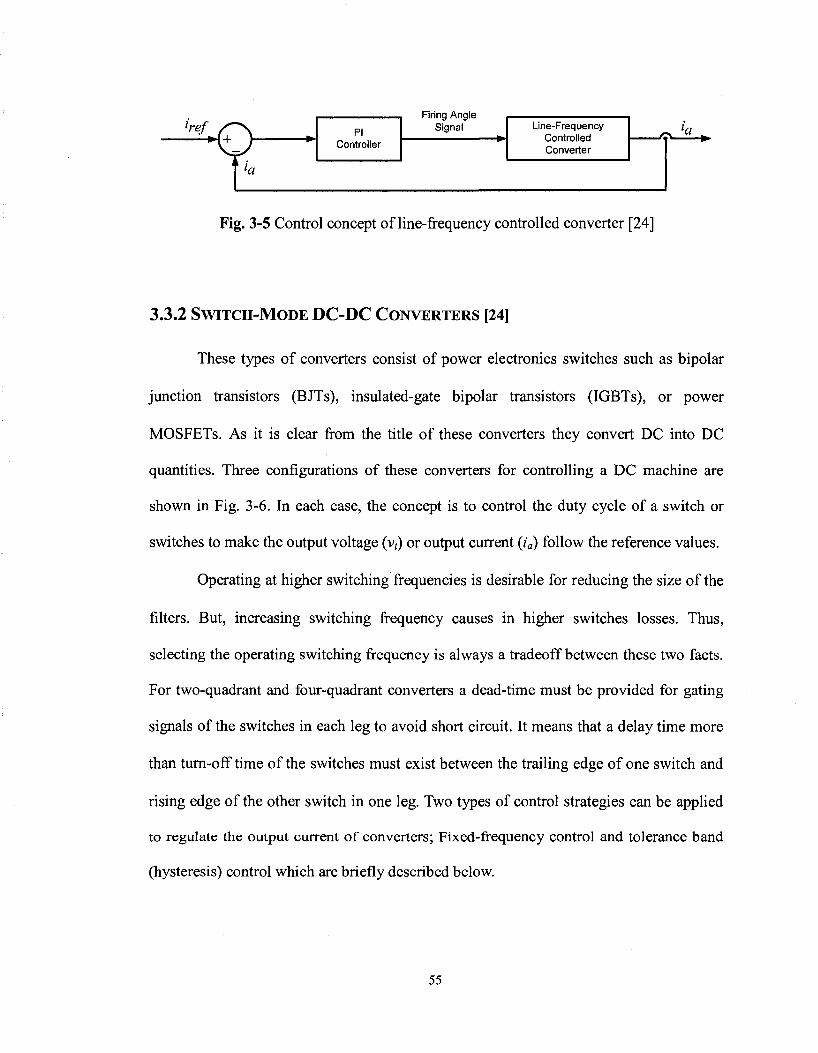
lref S~\ % ) -
"la
Fig. 3-5 Control concept of line-frequency controlled converter [24]
3.3.2 S W I T C H - M O D E DC-DC CONVERTERS [24]
These types of converters consist of power electronics switches such as bipolar
junction transistors (BJTs), insulated-gate bipolar transistors (IGBTs), or power
MOSFETs. As it is clear from the title of these converters they convert DC into DC
quantities. Three configurations of these converters for controlling a DC machine are
shown in Fig. 3-6. In each case, the concept is to control the duty cycle of a switch or
switches to make the output voltage (v,) or output current (ia) follow the reference values.
Operating at higher switching frequencies is desirable for reducing the size of the
filters. But, increasing switching frequency causes in higher switches losses. Thus,
selecting the operating switching frequency is always a tradeoff between these two facts.
For two-quadrant and four-quadrant converters a dead-time must be provided for gating
signals of the switches in each leg to avoid short circuit. It means that a delay time more
than turn-off time of the switches must exist between the trailing edge of one switch and
rising edge of the other switch in one leg. Two types of control strategies can be applied
to regulate the output current of converters; Fixed-frequency control and tolerance band
(hysteresis) control which are briefly described below.
PI Controller
Signal Line-Frequency Controlled Converter
55
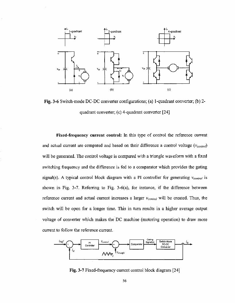
1-quadrant
-2
2-quadrant
4'
4-quadrant
-$
V«fc
i +
Vdc
?1 i V,
(a) (b) (c)
Fig. 3-6 Switch-mode DC-DC converter configurations; (a) 1-quadrant converter; (b) 2-
quadrant converter; (c) 4-quadrant converter [24]
Fixed-frequency current control: In this type of control the reference current
and actual current are compared and based on their difference a control voltage (vcontroi)
will be generated. The control voltage is compared with a triangle waveform with a fixed
switching frequency and the difference is fed to a comparator which provides the gating
signal(s). A typical control block diagram with a PI controller for generating vcontroi is
shown in Fig. 3-7. Referring to Fig. 3-6(a), for instance, if the difference between
reference current and actual current increases a larger v control will be created. Thus, the
switch will be open for a longer time. This in turn results in a higher average output
voltage of converter which makes the DC machine (motoring operation) to draw more
current to follow the reference current.
kef 0 PI Controller
^control Comparator
Gating Signal(s) Switch-Mode
DC-DC Converter
• ^ U
AAA* ' V triangle
Fig. 3-7 Fixed-frequency current control block diagram [24]
56
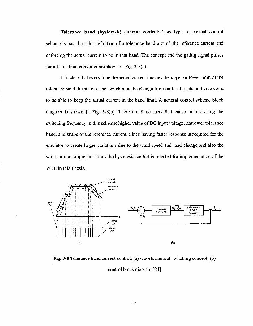
Tolerance band (hysteresis) current control: This type of current control
scheme is based on the definition of a tolerance band around the reference current and
enforcing the actual current to be in that band. The concept and the gating signal pulses
for a 1-quadrant converter are shown in Fig. 3-8(a).
It is clear that every time the actual current touches the upper or lower limit of the
tolerance band the state of the switch must be change from on to off state and vice versa
to be able to keep the actual current in the band limit. A general control scheme block
diagram is shown in Fig. 3-8(b). There are three facts that cause in increasing the
switching frequency in this scheme; higher value of DC input voltage, narrower tolerance
band, and shape of the reference current. Since having faster response is required for the
emulator to create larger variations due to the wind speed and load change and also the
wind turbine torque pulsations the hysteresis control is selected for implementation of the
WTE in this Thesis.
Switch /
(a)
Switch OFF
Hysteresis Controller
Gating Signal(s) Switch-Mode
DC-DC Converter
(b)
Fig. 3-8 Tolerance band current control; (a) waveforms and switching concept; (b)
control block diagram [24]
57

3.4 CONTROL LOGIC OF THE WTE [6]
Fig. 3-9 shows the schematic control logic of the WTE. This WTE represents a 2-
hp wind turbine since a 2-hp PMDC machine is used as the prime mover. It should be
noted that, the WTE can be used for wind turbines with higher power by employing
prime movers with higher ratings. The main concept is based on the fact that (referring to
Fig. 2-4) for a certain wind speed and certain wind turbine rotor speed (or equivalently
the prime mover speed by considering the gear ratio) there would be one and only one
torque on the stable region of the torque-speed characteristic.
The operating point, for a certain wind speed, on the torque-speed characteristic
depends on the load which wind turbine sees. Therefore, by imposing a load torque on
the shaft of the prime mover, the operating point of wind turbine will be established. To
impose a mechanical load torque on the shaft of the prime mover, a 2-hp PMDC machine
is used as dynamometer.
Thus, by measuring the dynamometer speed and feeding it back to wind turbine
model the reference torque for the prime mover will be created. The torque will be
converted to current which is called the prime mover reference current. On the other
hand, the actual current of the prime mover is measured. It will be compared with the
prime mover reference current through the prime mover hysteresis current controller and
the switching gating signals will be created.
58
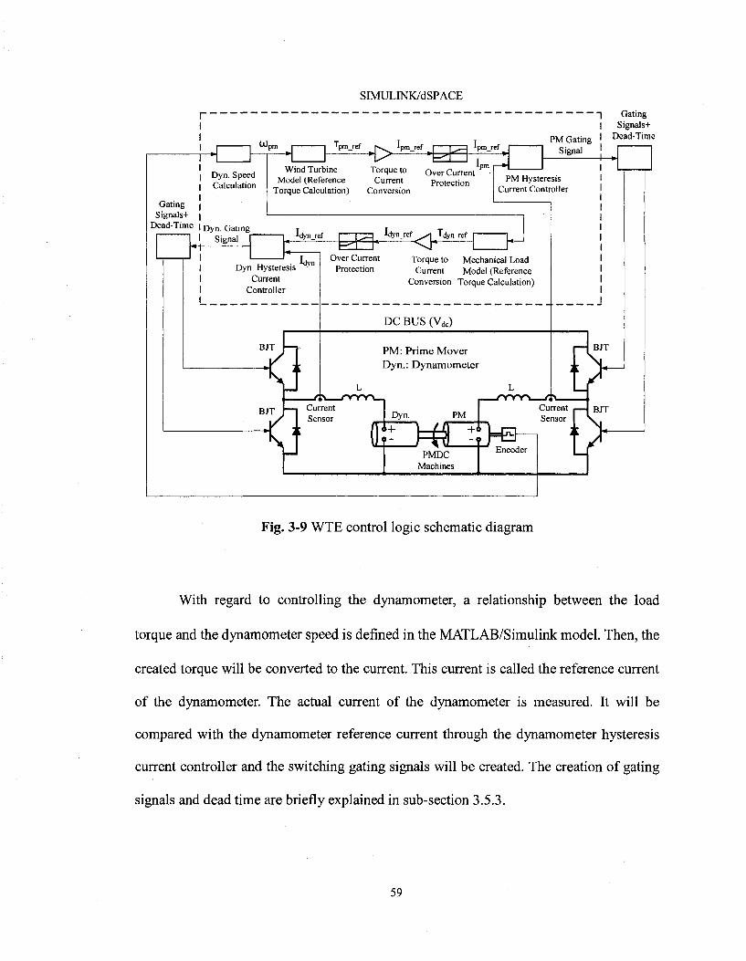
SIMULINK/dSPACE
Gating Signals+
Dead-Time
U), pm
Dyn. Speed Calculation
Dyn. Gating Signal
Tpm ref
•> pm_ref pm_ref
Wind Turbine Torque to Over Current Model (Reference Current Protection
Torque Calculation) Conversion
PM Gating Signal
"I Gating Signals+
Dead-Time
PM Hysteresis Current Controller
dyn_ref ldyn_ref ^ \ Tdynref
' <
Dyn. Hysteresis Current
Controller
Over Current Protection
Torque to Mechanical Load Current Model (Reference
Conversion Torque Calculation)
DC BUS (Vdc)
PM: Prime Mover Dyn.: Dynamometer
PM
C^hin PMDC
Machines
Encoder
Fig. 3-9 WTE control logic schematic diagram
With regard to controlling the dynamometer, a relationship between the load
torque and the dynamometer speed is defined in the MATLAB/Simulink model. Then, the
created torque will be converted to the current. This current is called the reference current
of the dynamometer. The actual current of the dynamometer is measured. It will be
compared with the dynamometer reference current through the dynamometer hysteresis
current controller and the switching gating signals will be created. The creation of gating
signals and dead time are briefly explained in sub-section 3.5.3.
59

3.5 EXPERIMENTAL SET-UP
Fig. 3-10 shows the experimental set-up which is used for implementing the
WTE. Two 2-hp PMDC machines are used as prime mover and dynamometer. Two 2-
quadrant switch-mode DC-DC converters are used for controlling the currents of the
machines. A 3-phase full bridge rectifier is used to provide the DC voltage for supplying
the power circuit of the prime mover and the dynamometer. A dSPACE ds-1103, a digital
controller for rapid prototyping that can be directly programmed with the simulink file
used for the simulation, is used. It is accompanied with a user interface, ControlDesk, for
operating, managing, and monitoring the experiments.
It should be noted that for the implemented WTE, a one-quadrant DC-DC
converter for the prime mover and a one-quadrant converter for the dynamometer circuit
will be suitable since the current direction in each circuit will remain the same. But,
actually a two-quadrant DC-DC converter has been used for each circuit. This provides
the opportunity for developing the proposed WTE for the future works as explained
below.
As it is noted in the literature, sometimes the generator will be used for the start
up of the wind turbine. Having two-quadrant switch-mode DC-DC converter provides the
opportunity to perform this task. In this case, the dynamometer will be used for starting
up the wind turbine by enforcing it to draw current in reverse direction. The prime mover,
in this case, will be enforced to draw current in the reverse direction to oppose the
dynamometer acting like wind turbine as a load for the generator.
The resistor, R, is used for discharging the capacitor for the time when the system
is not in use. Its value is 3.3 KX The capacitor, C, is used to reduce the ripple on the
60

rectifier output voltage. The inductors, L, are used to reduce the current rate of change of
the prime mover and the dynamometer in each simulation time step. The methods of
calculating values of the capacitor and inductors are described in the following sub
section.
DC BUS (Vdc)
Gating Signals Encoder To Switches Idyn Ipm Signal
1
Fig. 3-10 WTE experimental set-up
3.5.1 PARAMETERS SELECTION
Capacitor C: The value of the capacitor C is not a critical point in the design of
the WTE. Since the duty cycle of the switches will be automatically adjusted to provide
the required voltage for the DC machine as long as the DC bus voltage (Fdc) is greater
than the voltage required for the full load operation. But it is desirable to keep the voltage
ripple low around the average value of the DC bus voltage; because one of the factors of
emulating higher torques variations is to have a higher instantaneous voltage. Thus if the
61

voltage ripple will be high, it might be possible that at the time of step change in load the
instantaneous voltage will be much lower than its average value.
The detail of the calculation is not provided. But the calculations are done based
on , first, the theory and waveforms of the 3-phase full bridge diode rectifiers defined and
discussed in [24] and second, on the well known equations of the energy stored in a
capacitor which is E = 1/2CV and power and energy relationship E = Pt. Where E is the
stored energy in the capacitor in J, C is the capacitance of the capacitor in F, V is the
capacitor voltage in V, P is the load power in W, and t is the time which the capacitor
voltage drops from its maximum to minimum value in s. Therefore, considering that the
voltage variation will be between 230.5 and 229.5 V, the minimum capacitor's capacity
required to maintain this condition is 19,830 uF. The capacity of the capacitor which was
used in the experimental set-up was 21,600 uP.
Inductors L: The inductors are connected in series with the prime mover and
dynamometer to limit the rate of change of the current passing through the circuit. The
calculations will be provided for the prime mover circuit only since, the same logic can
be applied to the dynamometer circuit. Fig. 3-11 shows the prime mover circuit in two
operating conditions. Fig. 3-11(a) represents the condition when the upper switch is on,
this condition causes the current to rise. Fig. 3-11(b) represents the condition when the
lower switch is on, this condition causes the current to fall.
The value of Lt is the total reactance of the circuit (DC machine armature
reactance plus the reactance of inductor L). The value of Rt is the total resistance of the
circuit (DC machine armature resistance (0.855 Q) plus the resistance of the inductor L
(0.14 Q,). The voltage et is the back emf voltage plus 2 volts voltage drop due to the
62
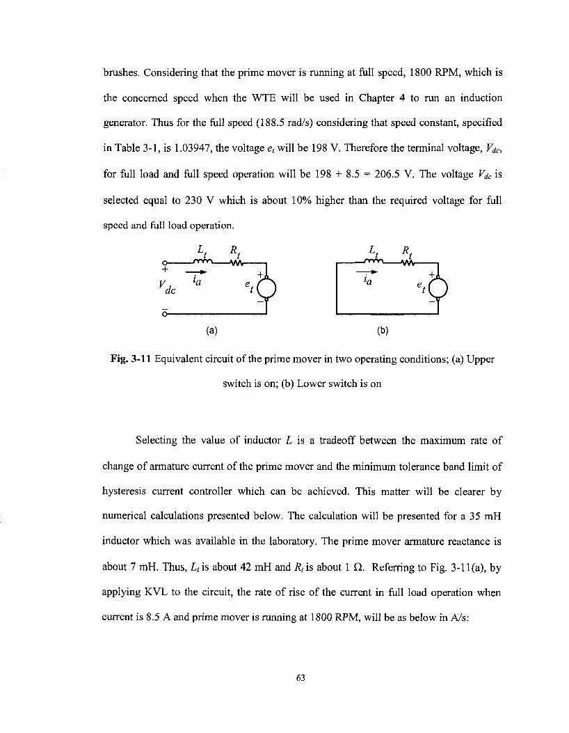
brushes. Considering that the prime mover is running at full speed, 1800 RPM, which is
the concerned speed when the WTE will be used in Chapter 4 to run an induction
generator. Thus for the full speed (188.5 rad/s) considering that speed constant, specified
in Table 3-1, is 1.03947, the voltage et will be 198 V. Therefore the terminal voltage, VdC,
for full load and full speed operation will be 198 + 8.5 = 206.5 V. The voltage Vdc is
selected equal to 230 V which is about 10% higher than the required voltage for full
speed and full load operation.
+ V la
etc
_rwr\ ^ mr*r» yy/v
la
(a) (b)
Fig. 3-11 Equivalent circuit of the prime mover in two operating conditions; (a) Upper
switch is on; (b) Lower switch is on
Selecting the value of inductor L is a tradeoff between the maximum rate of
change of armature current of the prime mover and the minimum tolerance band limit of
hysteresis current controller which can be achieved. This matter will be clearer by
numerical calculations presented below. The calculation will be presented for a 35 mH
inductor which was available in the laboratory. The prime mover armature reactance is
about 7 mH. Thus, Lt is about 42 mH and Rt is about 1 Q. Referring to Fig. 3-11(a), by
applying KVL to the circuit, the rate of rise of the current in full load operation when
current is 8.5 A and prime mover is running at 1800 RPM, will be as below in A/s:
63
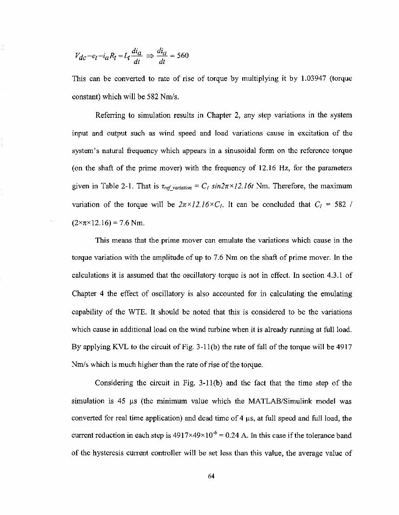
Vdc-et-iaRt=Lt^L ^ ^ = 560
This can be converted to rate of rise of torque by multiplying it by 1.03947 (torque
constant) which will be 582 Nra/s.
Referring to simulation results in Chapter 2, any step variations in the system
input and output such as wind speed and load variations cause in excitation of the
system's natural frequency which appears in a sinusoidal form on the reference torque
(on the shaft of the prime mover) with the frequency of 12.16 Hz, for the parameters
given in Table 2-1. That is xrefjariation = C; sin2K*12.16t Nm. Therefore, the maximum
variation of the torque will be 2KX12.16*CI. It can be concluded that C; = 582 /
(2x7ixl2.16) = 7.6 Nm.
This means that the prime mover can emulate the variations which cause in the
torque variation with the amplitude of up to 7.6 Nm on the shaft of prime mover. In the
calculations it is assumed that the oscillatory torque is not in effect. In section 4.3.1 of
Chapter 4 the effect of oscillatory is also accounted for in calculating the emulating
capability of the WTE. It should be noted that this is considered to be the variations
which cause in additional load on the wind turbine when it is already running at full load.
By applying KVL to the circuit of Fig. 3-11(b) the rate of fall of the torque will be 4917
Nra/s which is much higher than the rate of rise of the torque.
Considering the circuit in Fig. 3-11(b) and the fact that the time step of the
simulation is 45 jus (the minimum value which the MATLAB/Simulink model was
converted for real time application) and dead time of 4 ^s, at full speed and full load, the
current reduction in each step is 4917x49xl0"6 = 0.24 A. In this case if the tolerance band
of the hysteresis current controller will be set less than this value, the average value of
64

actual current will be less than the average value of the reference current. But the
tolerance band was actually set to 0.35 which is higher than calculated value. This
difference might be resulted from the discrepancies between measured or estimated
parameters with the real values such as DC machine armature resistance and inductance,
brushes voltage drop, and DC machine speed constant. If smaller inductor will be used, it
causes in higher rate of fall in current which means the tolerance band should be made
wider. One of the disadvantages of using wider tolerance band is that it results in higher
variations on the prime mover current which is not desirable when the machine is running
at full load.
3.5.2 METHODS OF USING MEASURED SPEED SIGNAL
Method-A (directly using measured speed signal): It is desirable to directly
(without filtering) use the speed signal for implementation of the WTE as shown in Fig.
3-9. This has been tried with 3 types of rotational speed measuring devices. Tachometer,
Optoschmitt sensor, and incremental encoder were used. The signal quality (high
variations or ripples around average value) of the first two devices did not let to emulate
wind turbines with the masses moment of inertias higher than 0.1 kgm2. For the values
above 0.1 kgm2, the created reference torque was boundlessly growing.
Therefore an incremental encoder with 3000 pulses/revolution was used to
overcome the problem. The incremental encoder typical speed signal (output) and its
frequency spectrum are shown in Fig. 3-12. The frequency spectrum of the speed signal
shows the nonzero magnitude for all frequencies. But ideally the only nonzero
component should be at 0 Hz, DC value. The largest magnitude (for nonzero frequencies)
65
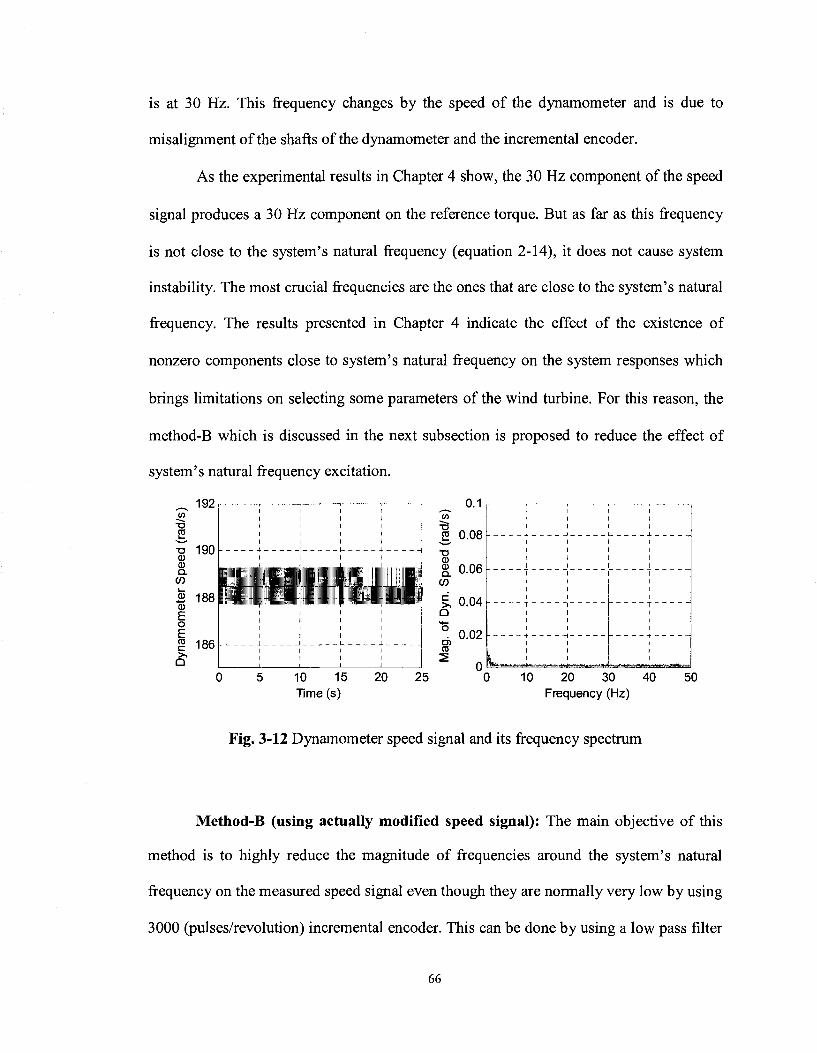
is at 30 Hz. This frequency changes by the speed of the dynamometer and is due to
misalignment of the shafts of the dynamometer and the incremental encoder.
As the experimental results in Chapter 4 show, the 30 Hz component of the speed
signal produces a 30 Hz component on the reference torque. But as far as this frequency
is not close to the system's natural frequency (equation 2-14), it does not cause system
instability. The most crucial frequencies are the ones that are close to the system's natural
frequency. The results presented in Chapter 4 indicate the effect of the existence of
nonzero components close to system's natural frequency on the system responses which
brings limitations on selecting some parameters of the wind turbine. For this reason, the
method-B which is discussed in the next subsection is proposed to reduce the effect of
system's natural frequency excitation.
192
190 E,
T J CD CD Q .
CD -I—»
CD E o E ? 186 Q
I
3 188 »
ll i l l I HjliPI 1
ll|! I J l , |
0.1
HI 41 Nl
E 0.08
CD
g. 0.06 CO
t 0.04 Q
CO 0.02
I I I I
I ' l l
T I T
l i
10 15 Time (s)
20 25 10 20 30 40 Frequency (Hz)
50
Fig. 3-12 Dynamometer speed signal and its frequency spectrum
Method-B (using actually modified speed signal): The main objective of this
method is to highly reduce the magnitude of frequencies around the system's natural
frequency on the measured speed signal even though they are normally very low by using
3000 (pulses/revolution) incremental encoder. This can be done by using a low pass filter
66
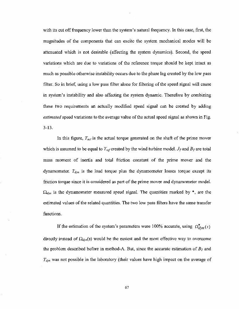
with its cut off frequency lower than the system's natural frequency. In this case, first, the
magnitudes of the components that can excite the system mechanical modes will be
attenuated which is not desirable (affecting the system dynamics). Second, the speed
variations which are due to variations of the reference torque should be kept intact as
much as possible otherwise instability occurs due to the phase lag created by the low pass
filter. So in brief, using a low pass filter alone for filtering of the speed signal will cause
in system's instability and also affecting the system dynamic. Therefore by combining
these two requirements an actually modified speed signal can be created by adding
estimated speed variations to the average value of the actual speed signal as shown in Fig.
3-13.
In this figure, Tact is the actual torque generated on the shaft of the prime mover
which is assumed to be equal to Tref created by the wind turbine model. Jr and Brave total
mass moment of inertia and total friction constant of the prime mover and the
dynamometer. Tdyn is the load torque plus the dynamometer losses torque except its
friction torque since it is considered as part of the prime mover and dynamometer model.
Qdyn is the dynamometer measured speed signal. The quantities marked by *, are the
estimated values of the related quantities. The two low pass filters have the same transfer
functions.
If the estimation of the system's parameters were 100% accurate, using Q*jyn(s)
directly instead of Qrfyn(s) would be the easiest and the most effective way to overcome
the problem described before in method-A. But, since the accurate estimation of Br and
Tdyn was not possible in the laboratory (their values have high impact on the average of
67
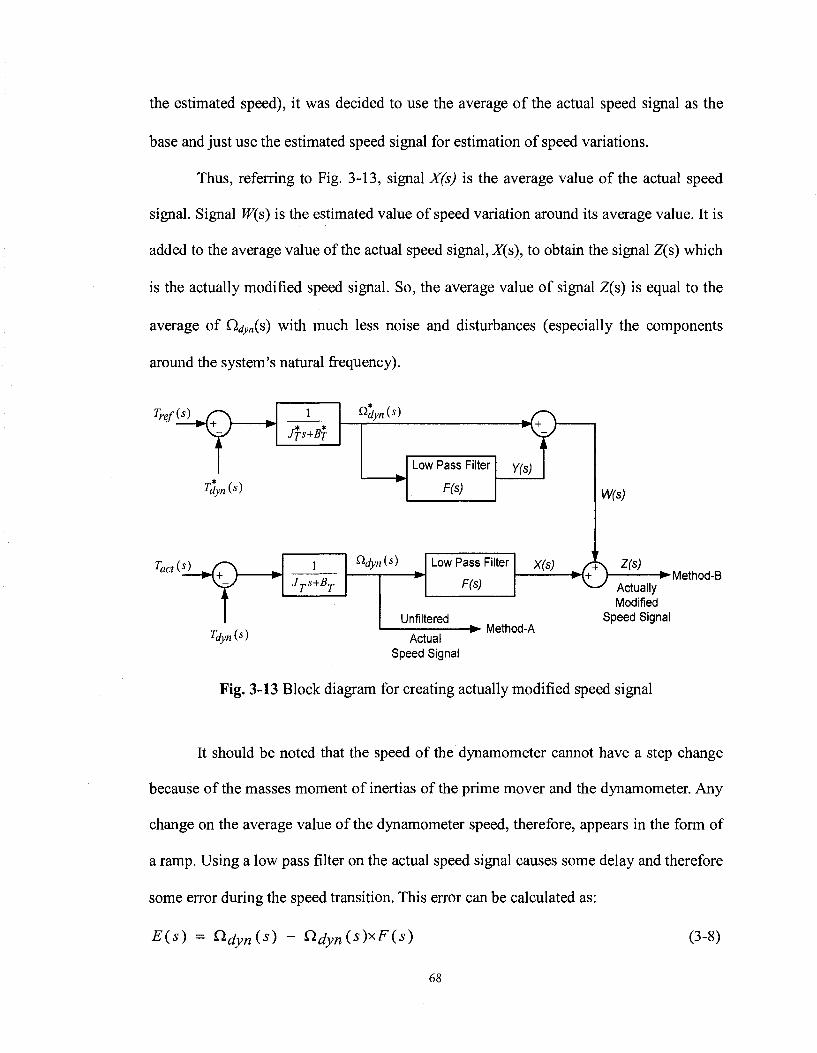
the estimated speed), it was decided to use the average of the actual speed signal as the
base and just use the estimated speed signal for estimation of speed variations.
Thus, referring to Fig. 3-13, signal X(s) is the average value of the actual speed
signal. Signal W(s) is the estimated value of speed variation around its average value. It is
added to the average value of the actual speed signal, X(s), to obtain the signal Z(s) which
is the actually modified speed signal. So, the average value of signal Z(s) is equal to the
average of O ^ s ) with much less noise and disturbances (especially the components
around the system's natural frequency).
Tref(s)
• 0 H+_ ) • r* n*
JfS+Bf
&dyn(s)
Q-
Tdyn 0s)
Low Pass Filter
F(s)
Y(s)
T^A_^Q. J rpS~Ti$rp
ndyn(s)
Tdyn^)
Low Pass Filter
F(s)
X(s)
W(s)
•6 Z(s)
-•Method-B
Unfiltered
Actual Speed Signal
- • Method-A
Actually Modified
Speed Signal
Fig. 3-13 Block diagram for creating actually modified speed signal
It should be noted that the speed of the dynamometer cannot have a step change
because of the masses moment of inertias of the prime mover and the dynamometer. Any
change on the average value of the dynamometer speed, therefore, appears in the form of
a ramp. Using a low pass filter on the actual speed signal causes some delay and therefore
some error during the speed transition. This error can be calculated as:
E(s) = Cldynis) - ndyn(s)xF(s) (3-8)
68
This error will be compensated by the signal W(s) as shown below:
W(s) = Cldyn(s) - n*dyn(s)xF(s) (3-9)
This is the estimated speed signal minus its filtered (average) value. Since the estimated
speed signal itself has some errors with respect to the actual speed signal, it brings some
limitations on reducing the cut off frequency of the low pass filter at will. In other words,
by inspecting equation 3-10 (based on Fig. 3-13), it is obvious that if
Q-dyn (s)=Cldyn (s), the signal Z(s) will be equal to Qdyn(s) independently of the transfer
function F(s).
Z(s) = Q*dyn(s) ~ tidyn(s) x F(*) + ^dyn(^) x ^(s) (3-10)
Experimental results show that as the cut off frequency of the low pass filters
were set to lower values the error between the estimated and actual speed signals
increased. It can be stated that the closer the estimated speed signal is to actual speed
signal, the lower is the cut off frequency of the low pass filters that can be used. The
other way of observing the problem of the error is that the time constant of the prime
mover and the dynamometer model is JJ/BT - 0.0203/0.0030725 = 6.6 s. Therefore, the
closer the time constant of the low pass filters is to the prime movers and the
dynamometer time constant the higher error is expected during the ramp transition of the
speed signal.
For the first order low pass filters, the time constant is inversely proportional to
the cut off frequency. Thus, to have less error (between estimated and actual speed signal)
the cut off frequency of the filter must be increased but by increasing the cut off
frequency the amount of the attenuation on the signals especially around system's natural
69
frequency will be reduced. Thus, the other option which is a second order filter is used
for two main reasons. First, attenuation of the frequencies higher than the cut off
frequency of the filter for the second order is higher. The attenuation is -40 dB/dec for a
second order filter and is -20 dB/dec for a first order filter. Second, for a specified cut off
frequency by changing the damping factor, the speed of the filter which is its rise time,
can be adjusted.
The second order low pass filters are discussed in detail in [28] and will be briefly
explained below. The general form of the transfer function of the second order low pass
filter is:
„2
S +2^Q)nS+COn
Where con = 2itfn in rad/s, fn is the natural frequency in Hz, and £ is the damping factor.
The rise time (time to go from 10% to 90% of the final value in s) of the filter is given as:
^ = 2.16^+0.6 o.3<£<0.8 (3-12)
Considering the above equations, it is possible to select the natural frequency for
enough attenuation of the frequencies above the cut off frequency and to reduce the value
of df for faster filter response for reducing the error during the transition. After extensive
tests the system responses were examined and the responses were acceptable for wide
ranges of the second order low pass filters in terms of their cut off frequencies and
damping factors. Thus, the experimental results in this Chapter and Chapter 4 are
provided for low pass filters with the following transfer function:
70

F(s)= ? {9K) - (3-13)
sz+5A7rs+(9xr
In equation 3-13, the natural frequency (fn) is 4.5 Hz and £is 0.3. Therefore, the rise time
is 0.044 s. The results will show that this filter provides enough attenuation around the
system's natural frequency for each case and also provides fast response so that the error
between the estimated and actual speed signals is not noticeable.
3.5.3 THE DSP SYSTEM [29]
Fig. 3-14 shows the input/output signals to and from ds-1103 control board. The
DSP development system which is used for implementation of the WTE is called
dSPACE. It has many features but the main features which are used for this experimental
set-up are briefly discussed here. By installing dSPACE it provides additional block-set
libraries in MATLAB/Simulink. One of them is the master PPC library which includes
ADC, DAC, and incremental encoder blocks.
ADC blocks are used in the MATLAB/Simulink model of the system to convert
analogue input signals to digital signals. The DAC blocks are used in the
MATLAB/Simulink model of the system to convert the signals created in the model to
analogue signals. The voltage levels that the ds-1103 can take as input signals and can
send as output signals are in the ±10 V range. The inputs/outputs on the ds-1103 board
are BNC connectors which provide easy and quick connections to other interface boards
via coaxial cables.
For this experimental set-up the outputs from dSPACE are only the gating signal
for each leg (prime mover switches and dynamometers switches). Since the maximum
71
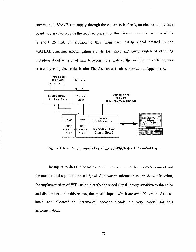
current that dSPACE can supply through these outputs is 5 mA, an electronic interface
board was used to provide the required current for the drive circuit of the switches which
is about 25 mA. In addition to this, from each gating signal created in the
MATLAB/Simulink model, gating signals for upper and lower switch of each leg
including about 4 |as dead time between the signals of the switches in each leg was
created by using electronic circuits. The electronic circuit is provided in Appendix B.
Gating Signals To Switches
A A A A tdyn t pm
Electronic Board+ Dead Time Circuit
Electronic Board
DAC
BNC Connectors
±10V
Encoder Signal 0-5 Volts
Differential Mode (RS-422)
ADC
BNC Connectors
±10 V
Encoders D-sub Connectors
dSPACEds-1103 Control Board
S1MULINK/ / dSPACE
CONTROL DbSK
Fig. 3-14 Input/output signals to and from dSPACE ds-1103 control board
The inputs to ds-1103 board are prime mover current, dynamometer current and
the most critical signal, the speed signal. As it was mentioned in the previous subsection,
the implementation of WTE using directly the speed signal is very sensitive to the noise
and disturbances. For this reason, the special inputs which are available on the ds-1103
board and allocated to incremental encoder signals are very crucial for this
implementation.
72

They are seven D-sub connector type inputs. Six of them accept encoder signals
in the form of digital signal and one of them accepts the signal of the encoder in the form
of analogue. Each input can be set to accept the signals in the form of single ended or
differential mode (RS-422). This can be done by placing the Encoder Master Setup block,
in the Master PPC library as mentioned before, in the Simulink model of the system. An
incremental encoder with 3000 pulses/revolution, with differential mode (RS-422) signals
and digital output, 0 - 5 V, was used. Special cable with twisted pairs with overall shield
and separate shield for each pair was used to minimize the noise on the signal.
After converting the Simulink model for real time application (by clicking the
build button), all the blocks in the model will be accessible by dSPACE/ Control Desk
software. This software provides many features such as measuring instrumentation,
sliders, control buttons, and data acquisition tools. All these, make it possible to change
the value of each block in the model while system is running (online), to observe the
waveforms at any point in the model, and to capture the data as m file, which can be used
in MATLAB for analysis or plotting.
3.5.4 MATLAB/SIMULINK MODEL
The MATLAB/Simulink model which was used for implementation of the
experimental set-up is shown in Fig. 3-15. It mainly consists of wind turbine model,
prime mover hysteresis current controller, prime mover measured current, dynamometer
hysteresis current controller, dynamometer measured current, dynamometer speed signal,
dynamometer measured current, and dynamometer torque estimation sub-system.
73
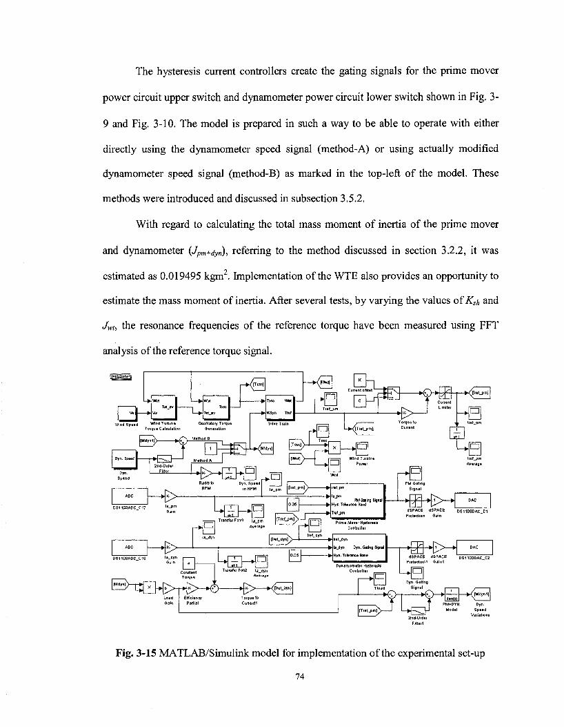
The hysteresis current controllers create the gating signals for the prime mover
power circuit upper switch and dynamometer power circuit lower switch shown in Fig. 3-
9 and Fig. 3-10. The model is prepared in such a way to be able to operate with either
directly using the dynamometer speed signal (method-A) or using actually modified
dynamometer speed signal (method-B) as marked in the top-left of the model. These
methods were introduced and discussed in subsection 3.5.2.
With regard to calculating the total mass moment of inertia of the prime mover
and dynamometer (Jpm+dyn), referring to the method discussed in section 3.2.2, it was
estimated as 0.019495 kgm2. Implementation of the WTE also provides an opportunity to
estimate the mass moment of inertia. After several tests, by varying the values of Ksh and
Jwt, the resonance frequencies of the reference torque have been measured using FFT
analysis of the reference torque signal.
Load Gain
Efficiency Partial
Torque to Current!
•1 (><Wn1]|
PM+DYN. Dyrv Model Speed
Variations
Fig. 3-15 MATLAB/Simulink model for implementation of the experimental set-up
74
Then, according to equation 2-14 corresponding Jpm+dyn were calculated in each
case. The average value of the measured Jpm+dyn was calculated as 0.0203 kgm . The error
between the average value and the values obtained in each case is less than 1.5 %. The
error between the estimated value of Jpm+dyn by the method introduced in Section 3.2.2,
0.019495 kgm2, and using WTE, 0.0203 kgm2, is about 4%. In Fig. 3-15, the "PM+Dyn.
Model" block is set equal to l/(0.0203s+0.0030725), where 0.0203 kgm2 and 0.0030725
Nms/rad are the estimated values for the total mass moment of inertia and the total
friction coefficient of the prime mover and the dynamometer, respectively.
In this model the created load torque is in the form of 7/00</ = bco . The value of b
in the experimental results is multiplied by the factor 0.94. The reason is the losses of
dynamometer, therefore, by reducing the load torque by that factor (0.94) the operating
points of the results in this Chapter (experimental results) are close to the operating points
of the results (simulation results) in Chapter 2. By doing this, comparison between the
experimental results and simulation results will be more straightforward.
In Fig. 3-15, there are two subsystems which are the prime mover and the
dynamometer hysteresis current controller. They are used to control the current of the
prime mover and of the dynamometer to follow their reference currents created in the
MATLAB/Simulink model. The models for both cases are nearly the same. Thus, the
prime mover hysteresis current controller is discussed here. This model was available in
the files of Mr. Avishek Mukherjee (former student in the electrical department) in the P.
D. Ziogas Power Electronics Laboratory, and with a slight change is used in this Thesis.
The model is shown in Fig. 3-16.
75
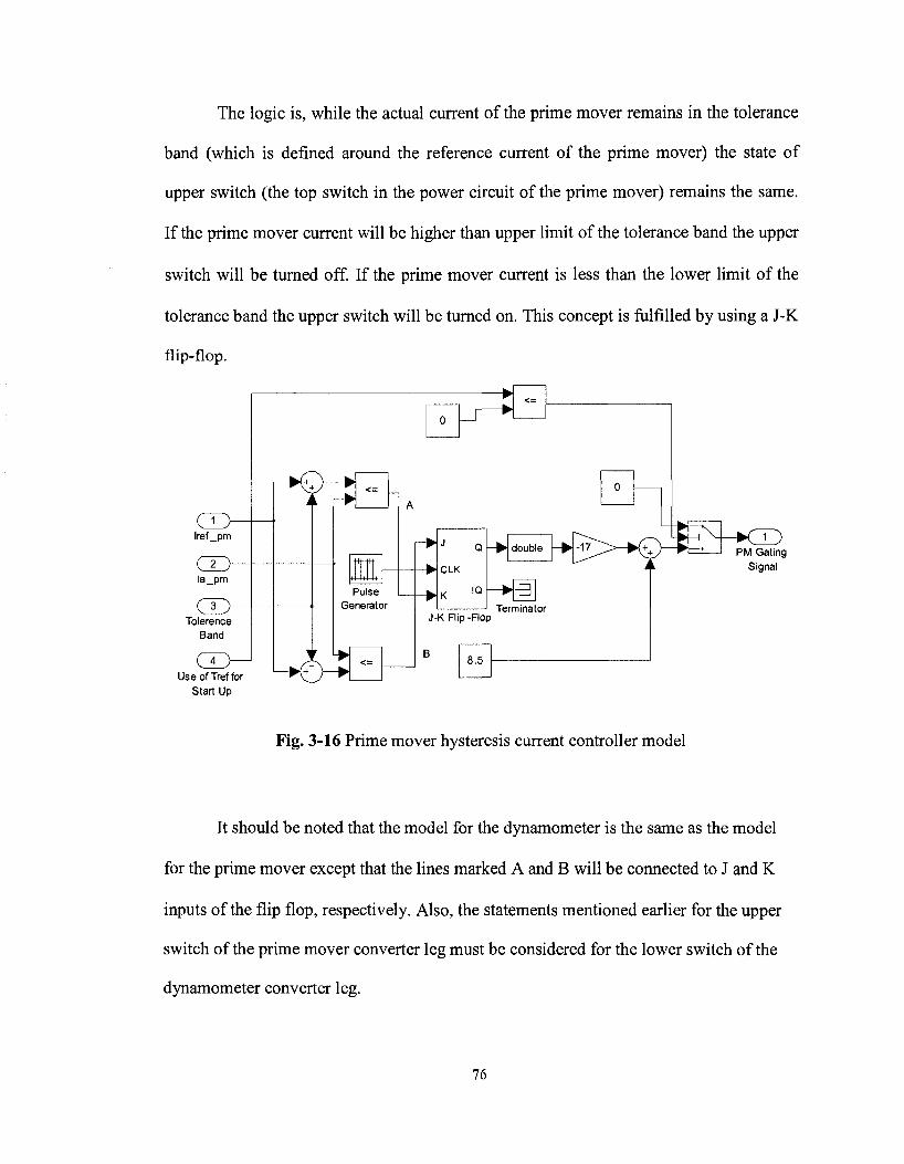
The logic is, while the actual current of the prime mover remains in the tolerance
band (which is defined around the reference current of the prime mover) the state of
upper switch (the top switch in the power circuit of the prime mover) remains the same.
If the prime mover current will be higher than upper limit of the tolerance band the upper
switch will be turned off. If the prime mover current is less than the lower limit of the
tolerance band the upper switch will be turned on. This concept is fulfilled by using a J-K
flip-flop.
lref_pm
la_pm
Tolerence Band
Use of Treffor Start Up
Pulse Generator
L -̂fl
CLK
K
double
-3
J-K Flip -Flop Terminator
8.5
PM Gating Signal
Fig. 3-16 Prime mover hysteresis current controller model
It should be noted that the model for the dynamometer is the same as the model
for the prime mover except that the lines marked A and B will be connected to J and K
inputs of the flip flop, respectively. Also, the statements mentioned earlier for the upper
switch of the prime mover converter leg must be considered for the lower switch of the
dynamometer converter leg.
76
3.6 EXPERIMENTAL RESULTS
Experimental results are provided in six different cases which include the steady-
state and transient responses. The conditions and parameters in all six cases are the same
as conditions and parameters in the cases shown in Chapter 2 (simulation results Section)
for ease of comparison between the experimental and simulation results. The parameters
for the experimental results are the same as the parameters in Table 2-1, unless otherwise
stated.
As it was discussed in Section 3.5.2, the WTE can be implemented by two
methods of using the dynamometer speed signal. Method-A (the speed signal is directly
used) and method-B (the actually modified speed signal is used). Since the results by two
methods are presented for all cases in Chapter 4 for comparison, to avoid lengthening the
Thesis, the results in this Chapter are provided for the case where method-B is used. The
reference torque (zrej) relates to the high speed torque (T^) and the dynamometer speed
(codyn) relates to the generator speed (cogen) in Chapter 2.
77

Case 1) This case highlights the effect of the wind turbine mass moment of inertia
on filtering of the oscillatory torque as far as generator torque and speed are concerned.
The results for this case are shown in Fig. 3-17 and are taken in steady-state. The wind
speed is constant at Vw = 8.25 m/s. The responses are shown for wind turbine with mass
moment of inertia (Jwt) equal to 1 and 10 kgm2. According to equation 2-18, the shaft
damping (Bsf,) are 0.7168 and 0.8120 Nms/rad, respectively.
The results show that the wind turbine and the dynamometer torque and speed
responses correspond to the results provided in the case 1 of simulation results in Chapter
2. In Fig. 3-17(b) the zoom of the dynamometer speed signals are presented to indicate
how close the actually modified speed signal and the actual speed signal are. In other
words, the reference torque creates the expected variations on the dynamometer speed.
Based on the results, it can be concluded that for the wind turbine with higher
mass moment of inertia the variations on the wind turbine rotor speed, reference torque
(dynamometer shaft), and the dynamometer speed are lower than the case where wind
turbine has lower mass moment of inertia. Higher mass moment of inertia can be
achieved at the expense of larger and heavier blades and consequently more expensive
wind turbine. Therefore, there should be a compromise in selecting wind turbine mass
moment of inertia and generated power.
78

46.5
8>
5.2 5.4 5.6 Time (s)
5.8
in 7 -.1 n « r . a
Ij!XiX±jTLi
185
uwt 1 Kgm^
5.2 5.4 5.6 5.8
5.4 5.6 Time (s)
"wt 10 Kgrrf
185
• D S
Actual
(a)
Modified
•o 50
•a S
185
184
183
5.75 Time(s)
182 5.5
(b)
Jw t=10Kgm 2
5.75 Time (s)
Fig. 3-17 Experimental results for case 1; (a) WTE responses; (b) Zoom of the
dynamometer speed signals
79

Case 2) This case highlights the effect of the wind turbine mass moment of inertia
on filtering of the wind speed variations as far as the generator torque and speed are
concerned. For power system studies, it is suggested in [19] to consider some harmonics
on the wind speed and the frequencies of the harmonics are in the range of 0.1 -10 Hz.
The results for this case are shown in Fig. 3-18.
The wind speed is considered to be Vw = 8.25 + 0.2 sinlnt + 0.2 sin6nt + 0.2
sin2QTxt m/s. The coefficients A and B of the oscillatory torque in equation 2-10 are set
equal to zero to be able to easily observe the effect of only wind speed variations on the
system responses. The responses are shown for wind turbine with mass moment of inertia
(Jwt) equal to 1 and 10 kgm2. According to equation 2-18, the shaft damping (Bsh) are
0.7168 and 0.8120 Nms/rad, respectively. The phase difference between the wind speed
profiles is due to the fact that the results for two cases are captured at different times. The
responses are shown in steady-state.
The results show that the wind turbine and the dynamometer torque and speed
responses correspond to the results provided in the case 2 of simulation results in Chapter
2. In Fig. 3-18(b) the zoom of the dynamometer speed signals are presented to indicate
that how close the actually modified speed signal and the actual speed signal are. In other
words, the reference torque creates the expected variations on the dynamometer speed.
The results reveal that the wind turbine produced torque is the same for both lower and
higher masses moment of inertias. But, the reference torque and the dynamometer speed
have lower variations for the wind turbine with higher mass moment of inertia.
80
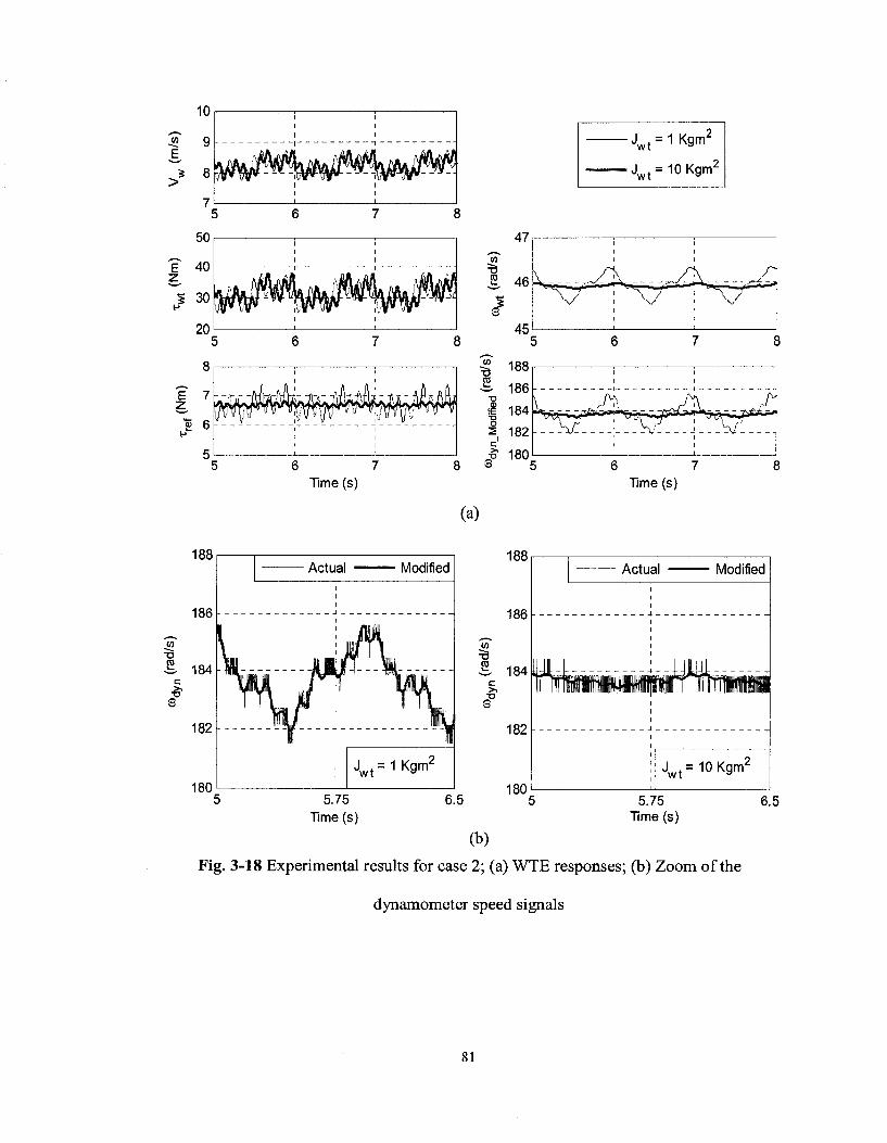
1 1 ! 1
1
5 6 7 8
1 1
1W% 5 6
1
1
7 8
1 1
A ll i A A
V '1/If " l/v * i l i l t 1
6 7 Time (s)
(a)
Actual
Jw t=1Kgm2
188
186
I 184 •D
s
5.75 Time (s)
6.5
182
180
(b)
J w t = 1 l W
•Jwt=10Kgm2
Til!
A - X . . - I 1 1 _ _ • ! £ _ - !
^ • > ^ W r -1JJJIL
nrTnffh«Mi
Jw t=10Kgm2
5.75 Time (s)
6.5
Fig. 3-18 Experimental results for case 2; (a) WTE responses; (b) Zoom of the
dynamometer speed signals
81
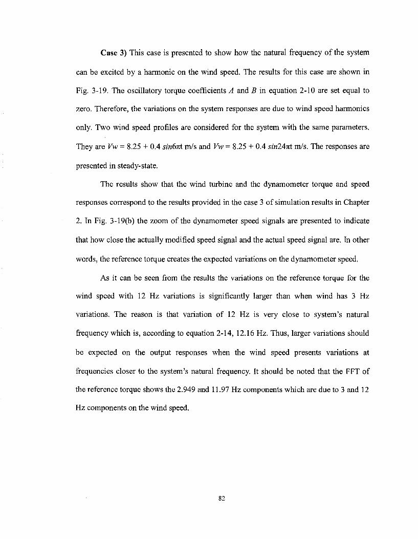
Case 3) This case is presented to show how the natural frequency of the system
can be excited by a harmonic on the wind speed. The results for this case are shown in
Fig. 3-19. The oscillatory torque coefficients A and B in equation 2-10 are set equal to
zero. Therefore, the variations on the system responses are due to wind speed harmonics
only. Two wind speed profiles are considered for the system with the same parameters.
They are Vw = 8.25 + 0.4 sin&itt m/s and Vw = 8.25 + 0.4 sin24iti m/s. The responses are
presented in steady-state.
The results show that the wind turbine and the dynamometer torque and speed
responses correspond to the results provided in the case 3 of simulation results in Chapter
2. In Fig. 3-19(b) the zoom of the dynamometer speed signals are presented to indicate
that how close the actually modified speed signal and the actual speed signal are. In other
words, the reference torque creates the expected variations on the dynamometer speed.
As it can be seen from the results the variations on the reference torque for the
wind speed with 12 Hz variations is significantly larger than when wind has 3 Hz
variations. The reason is that variation of 12 Hz is very close to system's natural
frequency which is, according to equation 2-14, 12.16 Hz. Thus, larger variations should
be expected on the output responses when the wind speed presents variations at
frequencies closer to the system's natural frequency. It should be noted that the FFT of
the reference torque shows the 2.949 and 11.97 Hz components which are due to 3 and 12
Hz components on the wind speed.
82
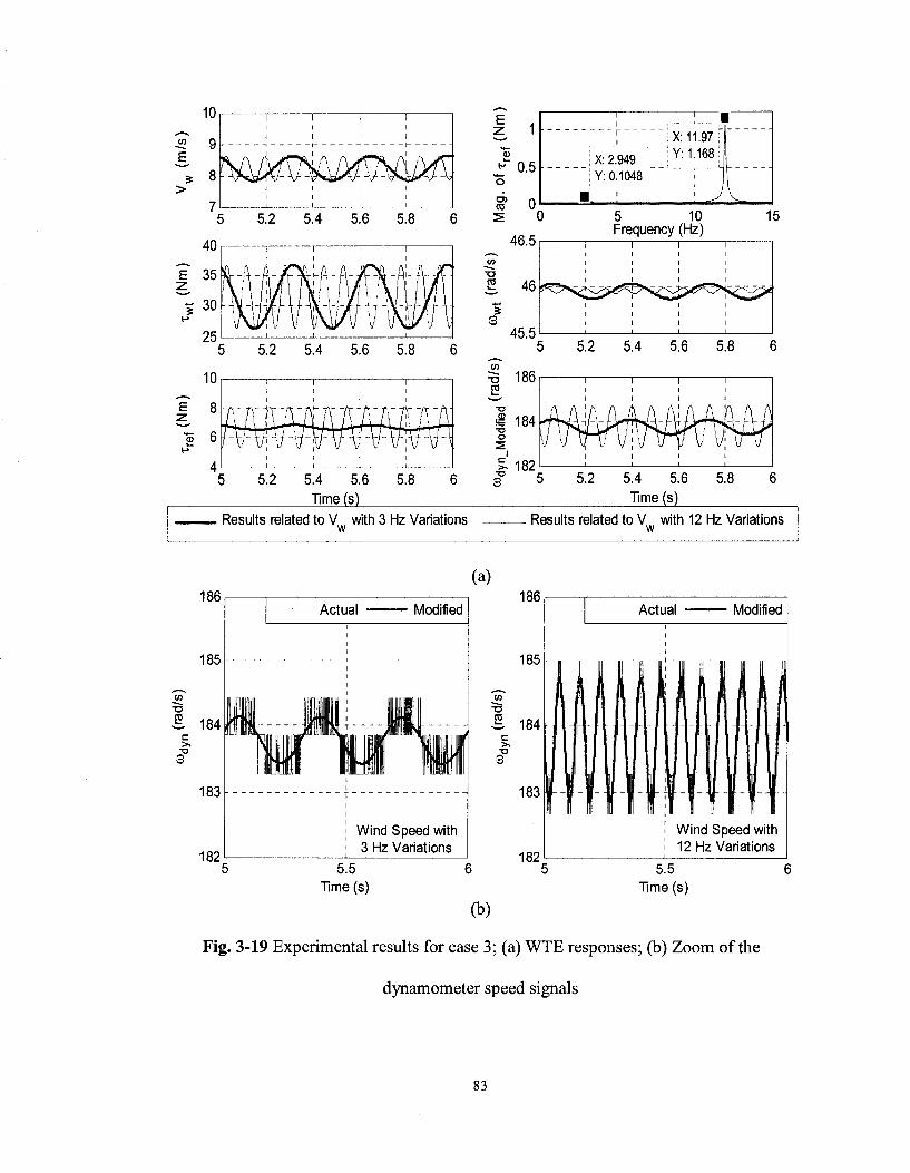
05
"E
s
5.4 5.6 Time (s)
^ 0.5 o
S* 0
46.5
X: 2.949 Y: 0.1048:
X: 11.97 Y: 1.168
5 10 Frequency (Hz)
5.4 5.6
Time (s)
15
Results related to V with 3 Hz Variations W
Results related to V with 12 Hz Variations w
182
Wind Speed with 3 Hz Variations
5.5 Time (s)
182
(b)
Actual Modified
Wind Speed with 12 Hz Variations
5.5 Time (s)
Fig. 3-19 Experimental results for case 3; (a) WTE responses; (b) Zoom of the
dynamometer speed signals
83
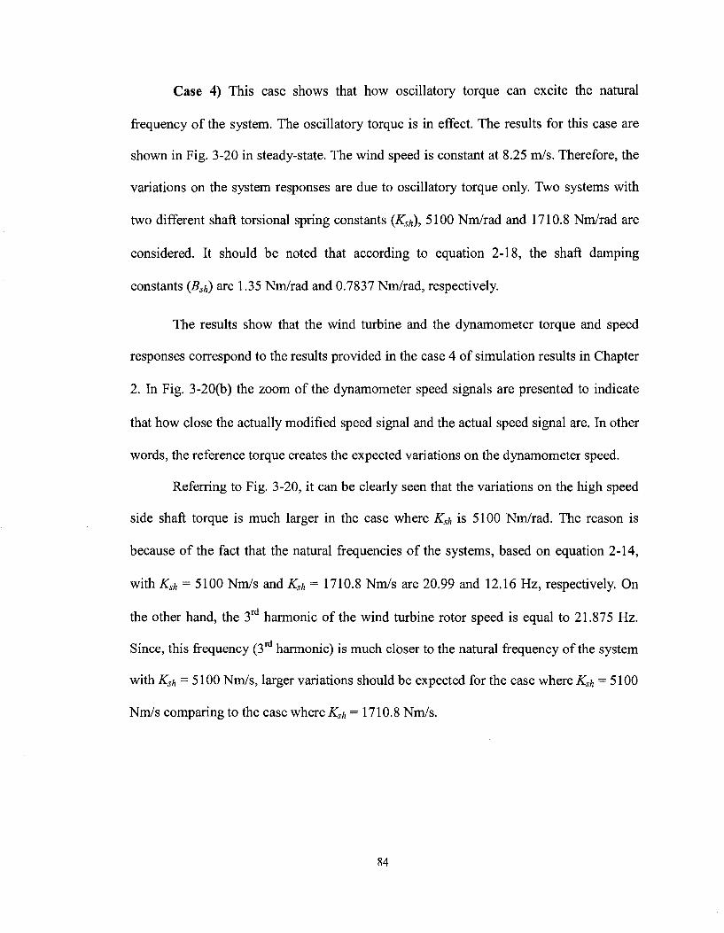
Case 4) This case shows that how oscillatory torque can excite the natural
frequency of the system. The oscillatory torque is in effect. The results for this case are
shown in Fig. 3-20 in steady-state. The wind speed is constant at 8.25 m/s. Therefore, the
variations on the system responses are due to oscillatory torque only. Two systems with
two different shaft torsional spring constants (KSh), 5100 Nm/rad and 1710.8 Nm/rad are
considered. It should be noted that according to equation 2-18, the shaft damping
constants (Bsh) are 1.35 Nm/rad and 0.7837 Nm/rad, respectively.
The results show that the wind turbine and the dynamometer torque and speed
responses correspond to the results provided in the case 4 of simulation results in Chapter
2. In Fig. 3-20(b) the zoom of the dynamometer speed signals are presented to indicate
that how close the actually modified speed signal and the actual speed signal are. In other
words, the reference torque creates the expected variations on the dynamometer speed.
Referring to Fig. 3-20, it can be clearly seen that the variations on the high speed
side shaft torque is much larger in the case where Ksh is 5100 Nm/rad. The reason is
because of the fact that the natural frequencies of the systems, based on equation 2-14,
with Ksh = 5100 Nm/s and Ksh = 1710.8 Nm/s are 20.99 and 12.16 Hz, respectively. On
the other hand, the 3rd harmonic of the wind turbine rotor speed is equal to 21.875 Hz.
Since, this frequency (3rd harmonic) is much closer to the natural frequency of the system
with KSh = 5100 Nm/s, larger variations should be expected for the case where Ksh = 5100
Nm/s comparing to the case where Ksh = 1710.8 Nm/s.
84
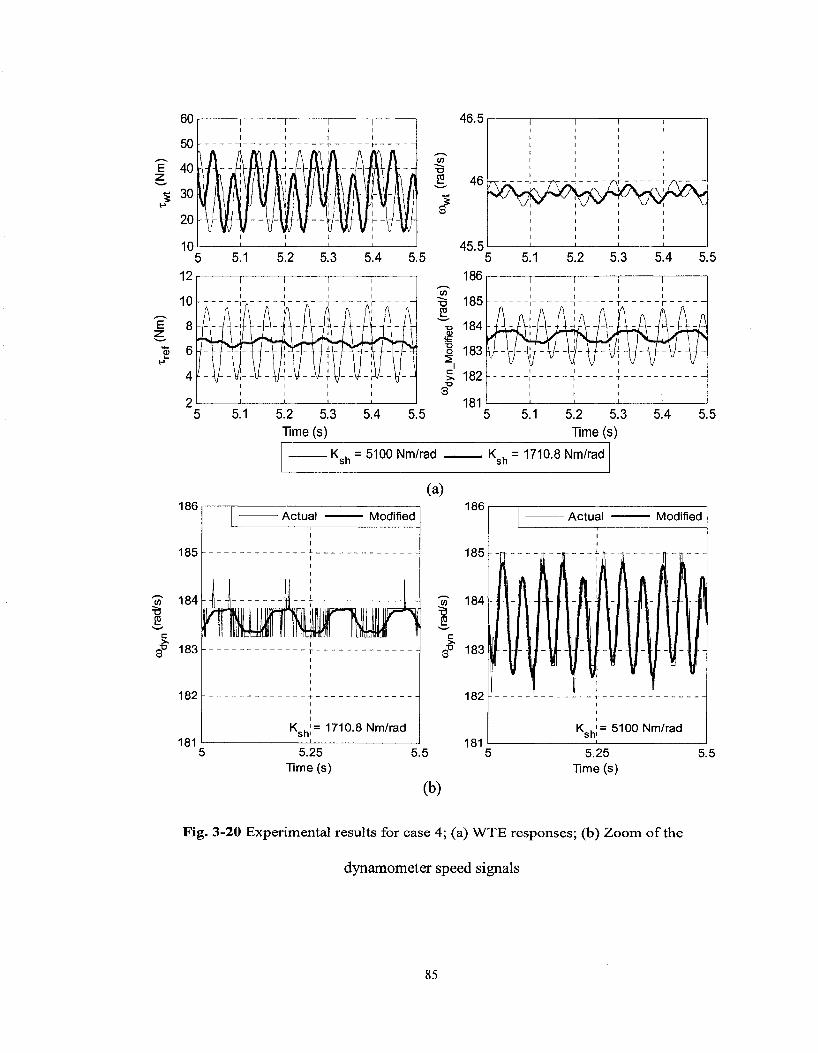
60
50
40
30
20 h
10
12
10
8
6
4
2
46.5
186
5.1
-u 50
IT 71"
L-\j--\!
I I I
f I T
--U--
J7N**"T /' / /1 W
]}-\ - v -
i
T 7 11 r
/ ' \ / H i
1
1 / n /
- f (-
u--^
fO
45.5
186
185
0) fB u o ^ c
X)
a
184
183
182
5.2 5.3 Time (s)
5.4 5.5 181
5.1 5.2 5.3 Time (s)
Ksh = 5100 Nm/rad Ksh= 1710.8 Nm/rad
(a) 186 r
5.4 5.5
_ ! j
A ' A A ' A 'A f\ A
5.4 5.5
5.25 Time (s)
5.25 Time (s)
(b)
Fig. 3-20 Experimental results for case 4; (a) W T E responses; (b) Zoom of the
dynamometer speed signals
85

Case 5) In this case the effect of wind speed step changes on the system responses
are investigated. It includes transient as well as steady-state responses. The results for this
case are shown in Fig. 3-21. The wind speed is selected at 8.85 m/s. The mechanical load
coefficient is b = 246 x 10"6 Nms2/rad2. The system responses are provided for the wind
turbines with two different masses moment of inertias, 3 and 7 kgm . According to
equation 2-18, the shaft damping constants equal to 0.7837 and 0.8065 Nms/rad are
considered, respectively. Fig. 3-21(a) shows the wind turbine responses, Fig. 3-21(b)
shows the dynamometer responses, and Fig. 3-21 (c) is the zoom of the reference torque.
The results show that the wind turbine and the dynamometer torque and speed responses
correspond to the results provided in the case 5 of the simulation results in Chapter 2.
The results show that the transient response for wind turbine with higher mass
moment of inertia is slower. Another point is that the wind speed change causes
overshoot or undershoot on the wind turbine torque and power responses but the other
responses such as wind turbine rotor speed and the generator side responses are under-
damped.
The other fact is that every time the wind speed changes, the system's mechanical mode
will be excited. This fact is shown in Fig. 3-21(c). The natural frequencies of the system
for Jwt equal to 3 and 7 kgm2, according to equation 2-14 are 12.16 and 11.81 Hz,
respectively. According to Fig. 3-21 (c), the calculated values of natural frequencies for
the wind turbines with the masses moment of inertias of 3 and 7 kgm2 are 12.19 and
11.79 Hz, respectively, which correspond to the theoretical values.
86
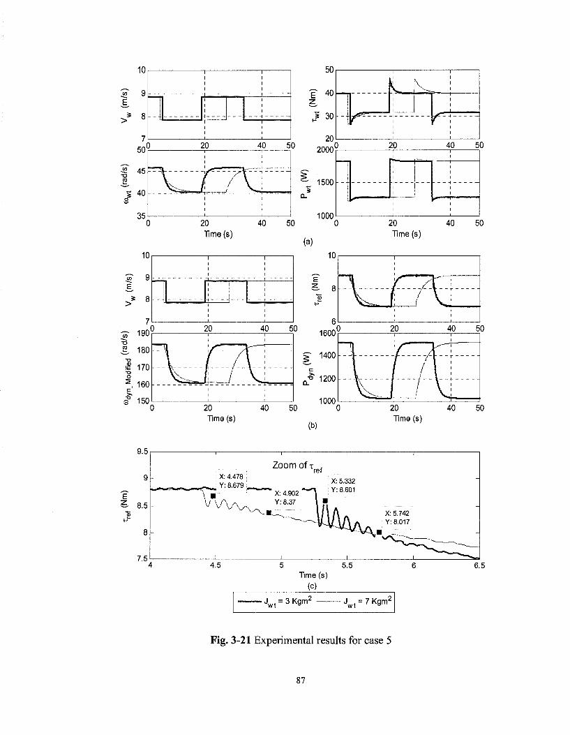
10
E
(rad
/s)
i
50
45
40
35
E
10
9
20
20 Time (s)
40 50
40 50
50
E" 40 \ z ? 30
20
2000
' 1500 3
1000
0
(a)
lr--
1
[s-J
k 1
20 Time (s)
20 40
20 Time (s)
40
50
> . 1,-F-n. • 1
I I
I )
I t
-| ( I I
*" '~i -** ''
50
E z .
<D H
8
R
1 1
i i
' l* r ">r" -\ / _ / ! _ _ ; \\ f / \ i v . Pi / \ i
! 1
Zoom of x
Time (s) (c)
J w t =3Kgm 2 - J , wt
= 7 Kgm2
Fig. 3-21 Experimental results for case 5
87

Case 6) This case is intended to investigate the effect of load step changes on the
system responses. It includes transient as well as steady-state responses. The results for
this case are shown in Fig. 3-22. The wind speed is selected at 8.5 m/s. The mechanical
load coefficient is b = 220 x 10"6 Nms2/rad2. The step changes in load are ± 40 * 10"6
Nms2/rad2. Fig. 3-22(a) shows the wind turbine responses, Fig. 3-22(b) shows the
dynamometer responses, and Fig. 3-22(c) is the zoom of the reference torque and
dynamometer speed signals.
The results show that the wind turbine and the dynamometer torque and speed
responses correspond to the results provided in the case 6 of simulation results in Chapter
2. In Fig. 3-22(b) the zoom of the dynamometer speed signals are presented to indicate
that how close the actually modified speed signal and the actual speed signal are. In other
words, the reference torque creates the expected variations on the dynamometer speed.
The importance of the load change, as it can be seen from the results, is the
excitation of the system's mechanical mode. Referring to equation 2-14 the natural
frequency of the system is 12.16 Hz. According to the points highlighted in Fig. 3-22(c)
the calculated natural frequency is 12.07 Hz which is very close to calculated theoretical
value. The other point is that the responses on the wind turbine side are all under-damped.
But, the load change causes overshoot or undershoot on the dynamometer torque and
power responses.
88
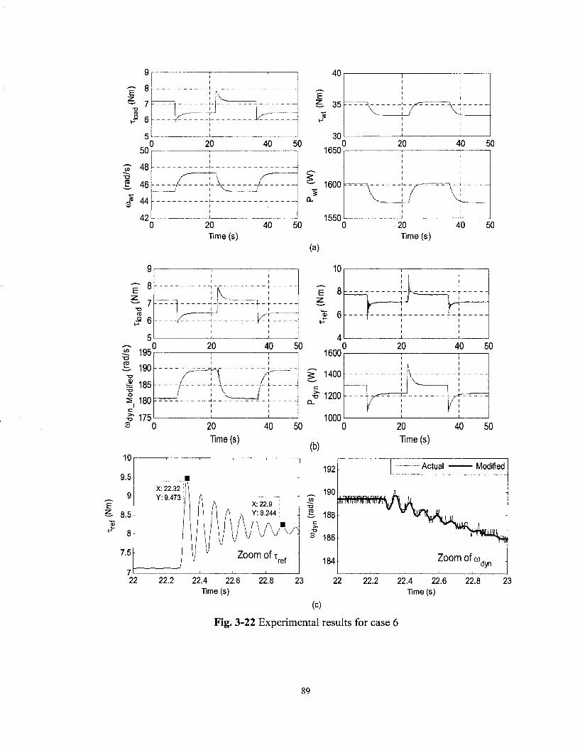
E 8
S 7 • o CO
f 6 5
50
£ 48
E. 46
S? 44
42
—--j-^^2 Ur_____:_
k ;
1 1
0 20 40 50 1 1
.....zzx \ / ! V
^ / i
: i
20 Time (s)
40 50
10r
9.5
9
8.5
8
7.5
! 1,
i ! 1
^
1
• X: 22.32 ill
: Y: 9.473
J ; j
A A X:22.9
A A Y:8-244 -
1 l/Wwv V Zoomoft re f -
192
190
I 188
3 186
22 22.2 22.4 22.6 22.8 Time (s)
20
20
Time (s)
40 50
-V""" 1 ._ — U I
40 50
lllilllmllKilM
« L 1 . > J - * J
Actual Modified
rffl
Zoom of co, dyn
184
23 22 22.2 22.4 22.6 22.8 Time (s)
23
(c)
Fig. 3-22 Experimental results for case 6
89

3.7 CONCLUSIONS
The focus of this chapter was on the implementation of a 2-hp WTE. The logic of
the WTE was introduced in Fig. 3-9. A 2-hp PMDC machine was used as prime mover. It
produces the torque equal to the reference torque on its shaft by using a switch-mode DC-
DC power converter and a hysteresis current controller. Another 2-hp PMDC machine
was used to operate as a dynamometer which acts as a mechanical load. It is supplied by
a switch-mode DC-DC power converter and a hysteresis current controller. This provided
the opportunity to make the WTE to run at different operating points to perform different
tests without requiring an electric generator and electrical load.
The experimental set-up was presented. The system parameters were calculated
and their effects on system limitations were discussed. Two methods (method-A and
method-B) of using the measured dynamometer speed signals were discussed, but the
results were shown for implementation with method-B only.
The main features of the designed and implemented WTE are:
> Capable of emulating the wind turbines with different mass moment of
inertias, drive train with flexible shaft with different torsional spring
constants, and damping constants, and ideal gear box with different gear
ratios.
> Capable of emulating the oscillatory torque.
> Provides the capability of experimentally verifying the facts highlighted in
the conclusion of Chapter 2 as simulation results.
90
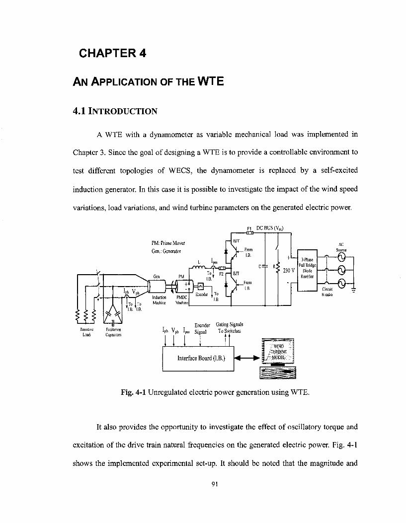
CHAPTER 4
AN APPLICATION OF THE WTE
4.1 INTRODUCTION
A WTE with a dynamometer as variable mechanical load was implemented in
Chapter 3. Since the goal of designing a WTE is to provide a controllable environment to
test different topologies of WECS, the dynamometer is replaced by a self-excited
induction generator. In this case it is possible to investigate the impact of the wind speed
variations, load variations, and wind turbine parameters on the generated electric power.
F1 DCBUS(V,ic) -CED-
PM: Prime Mover
Gen.: Generator
+ Gen. PM
U Vph
&
Induction PMDC T | B Induction PMDC
iTo iTo Machine Machine
M.B. IB.
Resistive Excitation Load Capacitors
Encoder Gating Signals Iph Vph Ipm signal To Switches
Fig. 4-1 Unregulated electric power generation using WTE.
It also provides the opportunity to investigate the effect of oscillatory torque and
excitation of the drive train natural frequencies on the generated electric power. Fig. 4-1
shows the implemented experimental set-up. It should be noted that the magnitude and
91
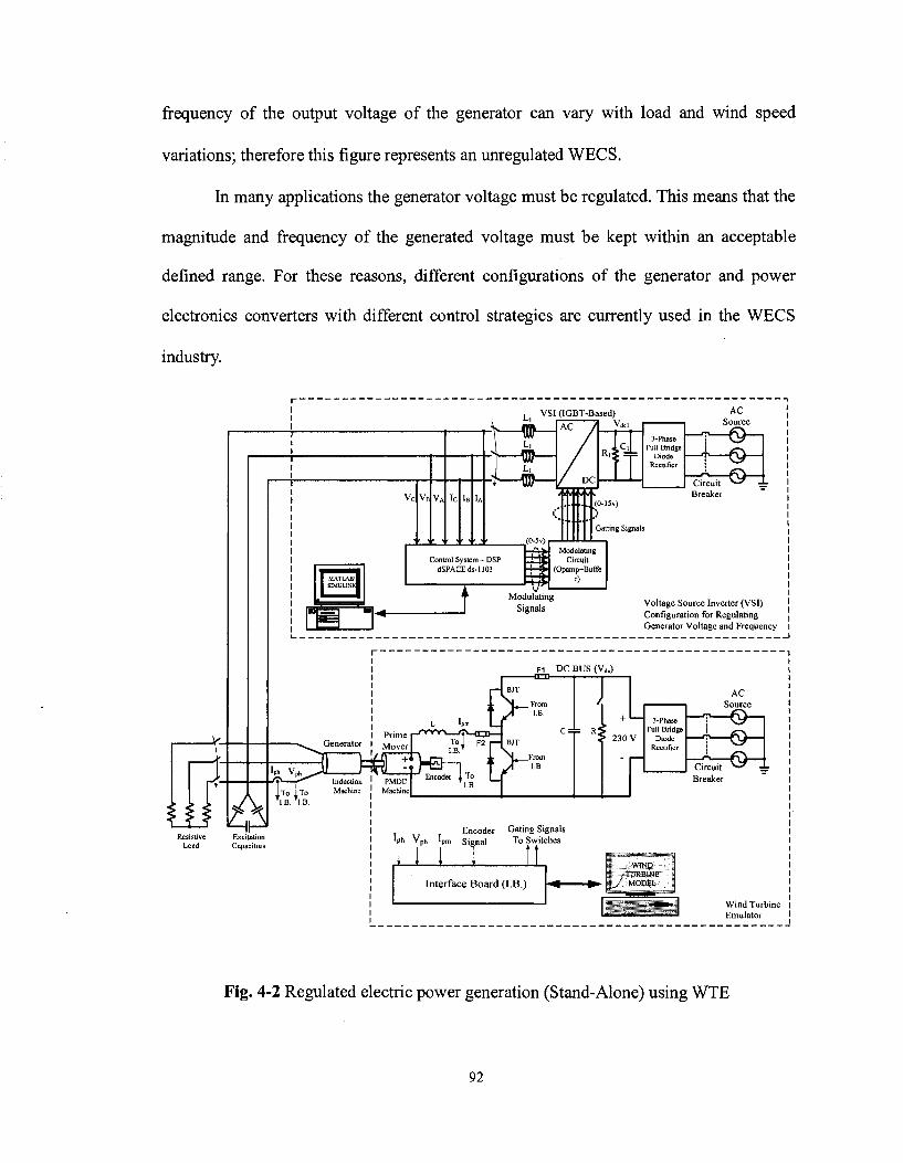
frequency of the output voltage of the generator can vary with load and wind speed
variations; therefore this figure represents an unregulated WECS.
In many applications the generator voltage must be regulated. This means that the
magnitude and frequency of the generated voltage must be kept within an acceptable
defined range. For these reasons, different configurations of the generator and power
electronics converters with different control strategies are currently used in the WECS
industry.
Resistive Load
Excitation Capacitors
Encoder Gating Signals Iph Vph Ipm Signal To Switches
1 1 1 1 Interface Board (I.B.)
Wind Turbine Emulator
Fig. 4-2 Regulated electric power generation (Stand-Alone) using WTE
92

The implemented WTE is also used as prime mover to run a 2-hp self-excited
induction generator in which its output power is controlled by a Voltage Source Inverter
(VSI). It represents a stand-alone regulated WECS. This topology is shown in Fig. 4-2.
The top part (VSI) was designed and implemented in [30]. The VSI is controlled in such
a way that it produces different amounts of power in order to maintain the generator
speed at its nominal value while wind speed and electrical load vary.
Section 4.2 provides some basic information about the induction generator and its
model. Section 4.3 describes the experimental set-up of the implemented WTE which
runs the induction generator in two cases; an unregulated WECS and a stand-alone
regulated WECS. The experimental results are presented in Section 4.4 and Section 4.5
summarizes this Chapter and presents the conclusions.
4.2 INDUCTION GENERATOR MODEL, PARAMETERS, AND
C H A R A C T E R I S T I C S [30,31]
To operate an induction machine as generator with rated voltage and frequency, it
must be run slightly over the synchronous speed. It needs reactive power which provides
the generator magnetization current [31]. In the case where it is connected to the grid, it
draws reactive power from the grid. In stand-alone applications, the reactive power must
be provided by a capacitor bank and/or by an inverter. A simplified, steady state, and per-
phase model of the induction generator as presented in [31] is shown in Fig. 4-3. In the
model, subscripts s and r correspond to stator and rotor parameters, respectively.
Subscript m corresponds to magnetization current and magnetization reactance. Vt and Vg
93
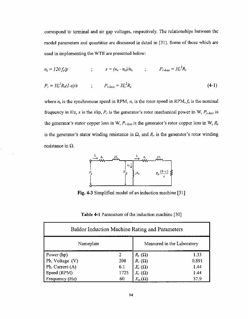
correspond to terminal and air gap voltages, respectively. The relationships between the
model parameters and quantities are discussed in detail in [31]. Some of those which are
used in implementing the WTE are presented below:
ns = 120 fs/p s = (ns- nr)/ns r-loss = 31/Rr
Pr = 3I/Rr(l-S)/S "s-loss 31s As (4-1)
where ns is the synchronous speed in RPM, nr is the rotor speed in RPM,^ is the nominal
frequency in Hz, s is the slip, Pr is the generator's rotor mechanical power in W, Ps.i0Ss is
the generator's stator copper loss in W, Pr-ioss is the generator's rotor copper loss in W, Rs
is the generator's stator winding resistance in Q, and Rr is the generator's rotor winding
resistance in Q..
R, )X* o WV rrvv"*-
4 Rr J*'
jX„ (\-s)
Fig. 4-3 Simplified model of an induction machine [31]
Table 4-1 Parameters of the induction machine [30]
Baldor Induction Machine Rating and Parameters
Nameplate
Power (hp) Ph. Voltage (V) Ph. Current (A) Speed (RPM) Frequency (Hz)
2 208 6.1 1725 60
Measured in the Laboratory
RsiO) Rr(Q) XS(Q) Xr(Q)
Xm(G)
1.33 0.891 1.44 1.44 37.9
94
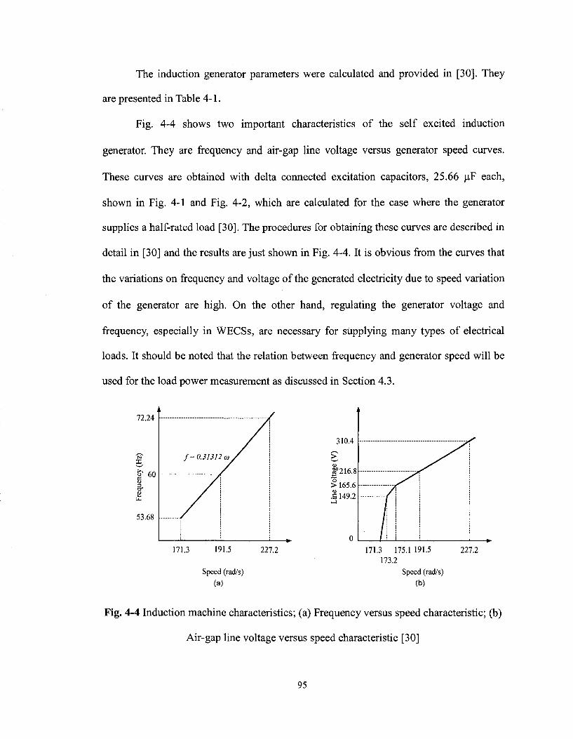
The induction generator parameters were calculated and provided in [30]. They
are presented in Table 4-1.
Fig. 4-4 shows two important characteristics of the self excited induction
generator. They are frequency and air-gap line voltage versus generator speed curves.
These curves are obtained with delta connected excitation capacitors, 25.66 uF each,
shown in Fig. 4-1 and Fig. 4-2, which are calculated for the case where the generator
supplies a half-rated load [30]. The procedures for obtaining these curves are described in
detail in [30] and the results are just shown in Fig. 4-4. It is obvious from the curves that
the variations on frequency and voltage of the generated electricity due to speed variation
of the generator are high. On the other hand, regulating the generator voltage and
frequency, especially in WECSs, are necessary for supplying many types of electrical
loads. It should be noted that the relation between frequency and generator speed will be
used for the load power measurement as discussed in Section 4.3.
72.24
s I 60 g-a
53.68
171.3 191.5 227.2 171.3 175.1 191.5 227.2
173.2
Speed (rad/s) Speed (rad/s)
(a) (b)
Fig. 4-4 Induction machine characteristics; (a) Frequency versus speed characteristic; (b)
Air-gap line voltage versus speed characteristic [30]
95
4.3 EXPERIMENTAL S E T - U P
All the discussions in the following subsections apply to both experimental set
ups, unregulated and regulated WECSs, shown in Fig. 4-1 and Fig. 4-2, respectively. The
system parameters, design methods, and implementation of the VSI configuration are
discussed in [30]. For this reason, in this section only the parts related to WTE are
described.
4.3.1 WTE PARAMETERS SELECTION
The values of R and C are equal to 3.3 kQ and 21,600 uF, respectively. These are
the same as those mentioned in Chapter 3. However, the value of L (the inductor in series
with the prime mover) differs from the value which has been selected in Chapter 3. The
reason is related to the sampling time of MATLAB/Simulink Model. Because of the
power measurement block which is added to the model, which contains time delay
blocks, the processing time of the DSP system increases. The minimum sampling time
that let the model to be converted for real time application was 70 jas.
By using the same method described in Chapter 3 and based on this new sampling
time, the value of L is selected to be equal to 48 mH. The total inductance is Lt = L + La
where L is the inductor in series with the DC machine and La is the armature inductance
of the DC machine. Therefore, the total inductance is Lt = 55 mH. The method discussed
in Chapter 3 for calculating the rate of rise and fall the torque which the DC machine will
be able to emulate can be applied to this Section. The DC bus voltage is selected as 230
V as mentioned in Chapter 3. Thus, for full load operation and rated generator speed the
96

prime mover will be able to follow the rate of rise of up to about 444 Nm/s and rate of
fall of up to about 3900 Nm/s.
Any time the wind speed or load suddenly changes, it causes a change on the
reference torque. Recall that this is the torque applied to the generator. The changes
appear in the form of damped sinusoidal (due to the excitation of the mechanical mode)
response until it reaches the steady-state condition. Therefore, a sudden or step change in
wind speed or load does not cause an instantaneous change on the reference torque. This
was verified by simulation results (Chapter 2) and experimental results (Chapter 3).
Having this in mind, the reference torque variations will be due to this fact plus the
variations due to 1st and 3rd harmonics of oscillatory torque. The worst case for having the
highest rate of rise on the reference torque is that the maximum rate of rise for the 1st and
3rd harmonics and the reference torque excitation occur simultaneously. The following
reference torque variation is considered:
Tref variation= Qsin(2x7.6;rt)+C2sin(2x22.8;rt)+C,3sin(2xl4.1;tf) (4-2)
Where 7.6, 22.8, and 14.1 are the frequencies of the 1st harmonic, 3rd harmonic, and the
system's natural frequency for Jwt = 1 kgm2, respectively. Assuming that C/ = 0.37 Nm
and C2 = 0.35 Nm which are the values shown in case 1 of the experimental results for Jwt
= 1 kgm2.
By differentiating equation 4-2, the maximum value will be reached when the
cosines are set equal to one. By doing this and equating equation 4-2 to 444 Nm/s
calculated before, C3 can be obtained equal to 4.25 Nm. This means that the WTE with
the selected parameters can emulate the variations on the wind speed and load which
cause excitation of the reference torque with the amplitude of up to 4.25 Nm. In the
97

calculations, it was considered that the generator operates at full load. If the generator
supplies lower load, the rate of rise of torque will be increased (due to less voltage drop
across DC motor armature resistance). It is worth saying that the prime mover full load
average torque is about 8.8 Nm.
The other fact which limits the reduction of the tolerance band limit is the amount
of current reduction in one simulation time step (70 us) and dead time of 4 us as
discussed in Chapter 3. This happens when the lower switch in Fig. 4-1 is on.
Considering that the prime mover is running at 1800 RPM and at full load condition (8.5
A), referring to Fig. 3-11(b) and the equation: A V = LtAia/Atsampimg, the current reduction
can be calculated: Aia = 206.5x74x10"6/(55xl0"3) = 0.28 A. For the same reason
discussed in Chapter 3 the tolerance band limit has to be greater than 0.28 A which is
thus selected equal to 0.35 A.
4.3.2 MATLAB/SIMULINK MODEL
The MATLAB/Simulink model used in the implementation of the experimental
set-up is shown in Fig. 4-5. It mainly consists of the wind turbine model, the prime mover
hysteresis current controller, the prime mover measured current, the generator speed
signal, the generator measured phase voltage and current, and the power measurement
block. The hysteresis current controller creates the gating signals for the prime mover
power circuit upper switch. By using external electronic circuits, gating signals with
appropriate power levels are created for both switches as discussed in Chapter 3. The
model is prepared to be able to operate with directly using of generator speed signal
98
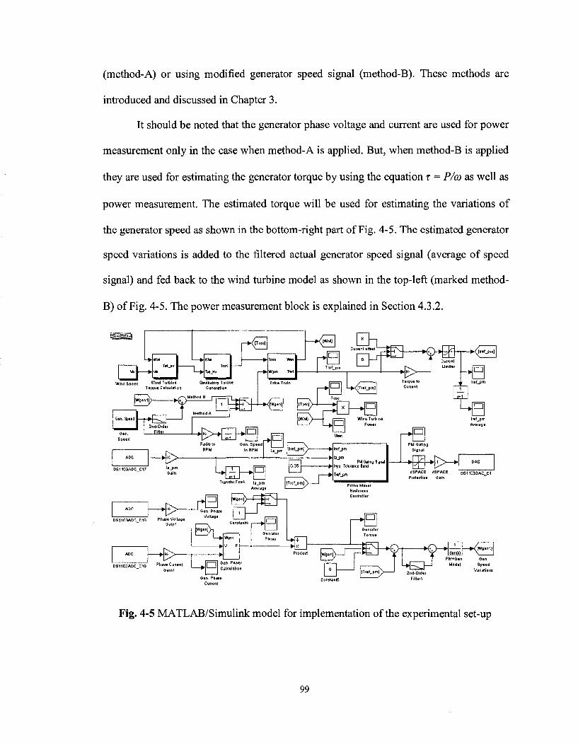
(method-A) or using modified generator speed signal (method-B). These methods are
introduced and discussed in Chapter 3.
It should be noted that the generator phase voltage and current are used for power
measurement only in the case when method-A is applied. But, when method-B is applied
they are used for estimating the generator torque by using the equation T = P/co as well as
power measurement. The estimated torque will be used for estimating the variations of
the generator speed as shown in the bottom-right part of Fig. 4-5. The estimated generator
speed variations is added to the filtered actual generator speed signal (average of speed
signal) and fed back to the wind turbine model as shown in the top-left (marked method-
B) of Fig. 4-5. The power measurement block is explained in Section 4.3.2.
Model Speed
Variations
Fig. 4-5 MATLAB/Simulink model for implementation of the experimental set-up
99
With regard to calculating the total mass moment of inertia of the DC motor and
induction generator (Jpm+gen) and total friction coefficient of the DC motor and induction
generator, referring to the method discussed in Chapter 3, they were estimated 0.0185
kgm2 and 0.00245 Nms/rad, respectively. The implementation of the WTE also provides
an opportunity to estimate the total mass moment of inertia of the prime mover (DC
motor) and the generator. After several tests, by varying the values of Ksh and Jwt,
resonance frequencies of the reference torque have been measured using FFT analysis of
the reference torque. Then, according to equation 2-14, corresponding Jpm+gen were
calculated in each case. The average value of the measured Jpm+gen was calculated as
0.0174 kgm2. The error of the average value is less than 1% for all cases. The estimated
values which are 0.0185 and 0.0174 kgm2 have an error of about 6% with respect to each
other. Therefore, in Fig. 4-5 the "PM+Gen. Model" block is set equal to
1/(0.0174s+0.00245), where 0.0174 kgm2 and 0.00245 Nms/rad are the estimated values
for the total mass moment of inertia and the total friction coefficient of the DC machine
and the induction machine, respectively.
4.3.3 POWER MEASUREMENT BLOCK
The power measurement block which is available in the MATLAB/Simulink
power systems library (version 5.3 of MATLAB) measures the power associated with the
input current and voltage to the block for the specific frequency. That frequency, for
instance 60 Hz, must be set in the block. Because the generator speed might vary
(unregulated operation) the frequency of the generator voltage changes in different
conditions. For this reason the power measurement block is slightly modified by using
100
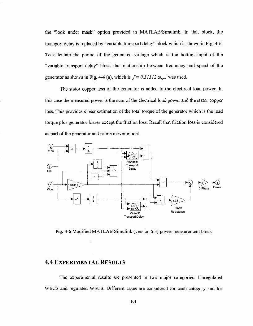
the "look under mask" option provided in MATLAB/Simulink. In that block, the
transport delay is replaced by "variable transport delay" block which is shown in Fig. 4-6.
To calculate the period of the generated voltage which is the bottom input of the
"variable transport delay" block the relationship between frequency and speed of the
generator as shown in Fig. 4-4 (a), which is / = 0.31312 cogen was used.
The stator copper loss of the generator is added to the electrical load power. In
this case the measured power is the sum of the electrical load power and the stator copper
loss. This provides closer estimation of the total torque of the generator which is the load
torque plus generator losses except the friction loss. Recall that friction loss is considered
as part of the generator and prime mover model.
© Vph
Iph
Wgen
ru Variable
Transport Delay
^ _ _ . Otwma
Variable Transport Delay 1
1.33
Stator Resistance
3 Phase Power
Fig. 4-6 Modified MATLAB/Simulink (version 5.3) power measurement block
4.4 EXPERIMENTAL RESULTS
The experimental results are presented in two major categories: Unregulated
WECS and regulated WECS. Different cases are considered for each category and for
101
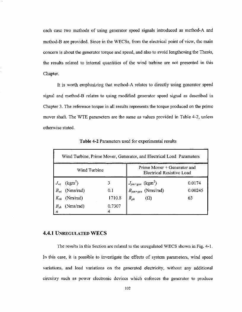
each case two methods of using generator speed signals introduced as method-A and
method-B are provided. Since in the WECSs, from the electrical point of view, the main
concern is about the generator torque and speed, and also to avoid lengthening the Thesis,
the results related to internal quantities of the wind turbine are not presented in this
Chapter.
It is worth emphasizing that method-A relates to directly using generator speed
signal and method-B relates to using modified generator speed signal as described in
Chapter 3. The reference torque in all results represents the torque produced on the prime
mover shaft. The WTE parameters are the same as values provided in Table 4-2, unless
otherwise stated.
Table 4-2 Parameters used for experimental results
Wind Turbine, Prime Mover, Generator, and Electrical Load Parameters
Wind Turbine
Jwt (kgm2) 3
Bwt (Nms/rad) 0.1
Ksh (Nm/rad) 1710.8
Bsh (Nms/rad) 0.7307 n 4
Prime Mover + Generator and Electrical Resistive Load
Jpm+gen (kgm2) 0.0174
Bpm+gen (Nms/rad) 0.00245
RPh (A) 63
4.4.1 UNREGULATED WECS
The results in this Section are related to the unregulated WECS shown in Fig. 4-1.
In this case, it is possible to investigate the effects of system parameters, wind speed
variations, and load variations on the generated electricity, without any additional
circuitry such as power electronic devices which enforces the generator to produce
102
electricity with constant voltage and frequency. Six different cases (steady-state and
transient responses) are discussed in this section.
Case 1) In this case the effect of the wind turbine mass moment of inertia on
suppressing the variations due to the oscillatory torque is investigated. The results for this
case are shown in Fig. 4-7 and Fig. 4-8 for method-A and method-B, respectively. The
system is tested for two values of Jwt equal to 1 and 10 kgm . According to equation 2-18,
the values of Bsh related to each Jwt are calculated and set to 0.6756 and 0.7534 Nms/rad,
respectively. The results are shown in the steady-state condition. The wind speed is kept
constant at 7.87 m/s at which the generator generates 120 V, rated phase voltage, at half-
rated load. Therefore, the variations on the reference torque should be due to the
oscillatory torque (1st and 3rd harmonics) only.
With regard to the results related to method-B, the generator speed (cogen_ACtuad,
represents the speed signal which is measured directly without any filtering. The
generator speed {cogen_Modifled), represents the speed signal with its variations estimated by
the model of the prime mover and generator and its average is the average of the
measured speed signal as discussed in Chapter 3.
The generator speed is about 190 rad/s. By dividing the generator speed by the
gear ratio the wind turbine rotor speed is 47.5 rad/s and the rotating frequency is equal to
7.56 Hz. Therefore, the frequency of 1st harmonic of the oscillatory torque is 7.56 Hz and
the frequency of its 3rd harmonic is 22.68 Hz. The frequency spectra of the reference
torque and generator speed are shown in Fig. 4-7(b) and (c) and Fig. 4-8(b), (c), and (d).
Referring to Fig. 4-7(b) and (c), the components of the oscillatory torque are at 7.628 and
103
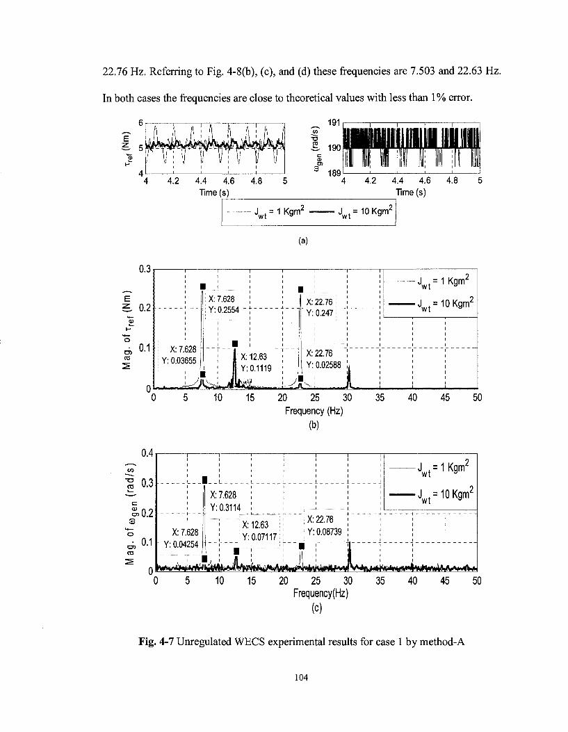
22.76 Hz. Referring to Fig. 4-8(b), (c), and (d) these frequencies are 7.503 and 22.63 Hz.
In both cases the frequencies are close to theoretical values with less than 1% error.
191
I 1901
4.2 4.4 4.6 4.8 Time (s)
Jwt=1Kgm2
(a)
189
Jwt=10Kgm^
4.2 4.4 4.6 4.8 Time (s)
20 25 30 35
Frequency (Hz)
(b)
40 45 50
CO
0.4
0.3
£0.2 s o
CO
0.1
___•__!_
1
X: 7.628
Y:0.04 i
X: 7.628 Y: 0.3114
j : X: 12.63 ! Y: 0.07117
ddkdkw kMM* 5 -<
><
I I
;
22.76 } ] 0.08739;
JLi
- J =1 wt
Kgm2
J w t = 10Kgm2
4M*t*w^
10 15 20 25 30 Frequency(Hz)
(c)
35 40 45 50
Fig. 4-7 Unregulated WECS experimental results for case 1 by method-A
104
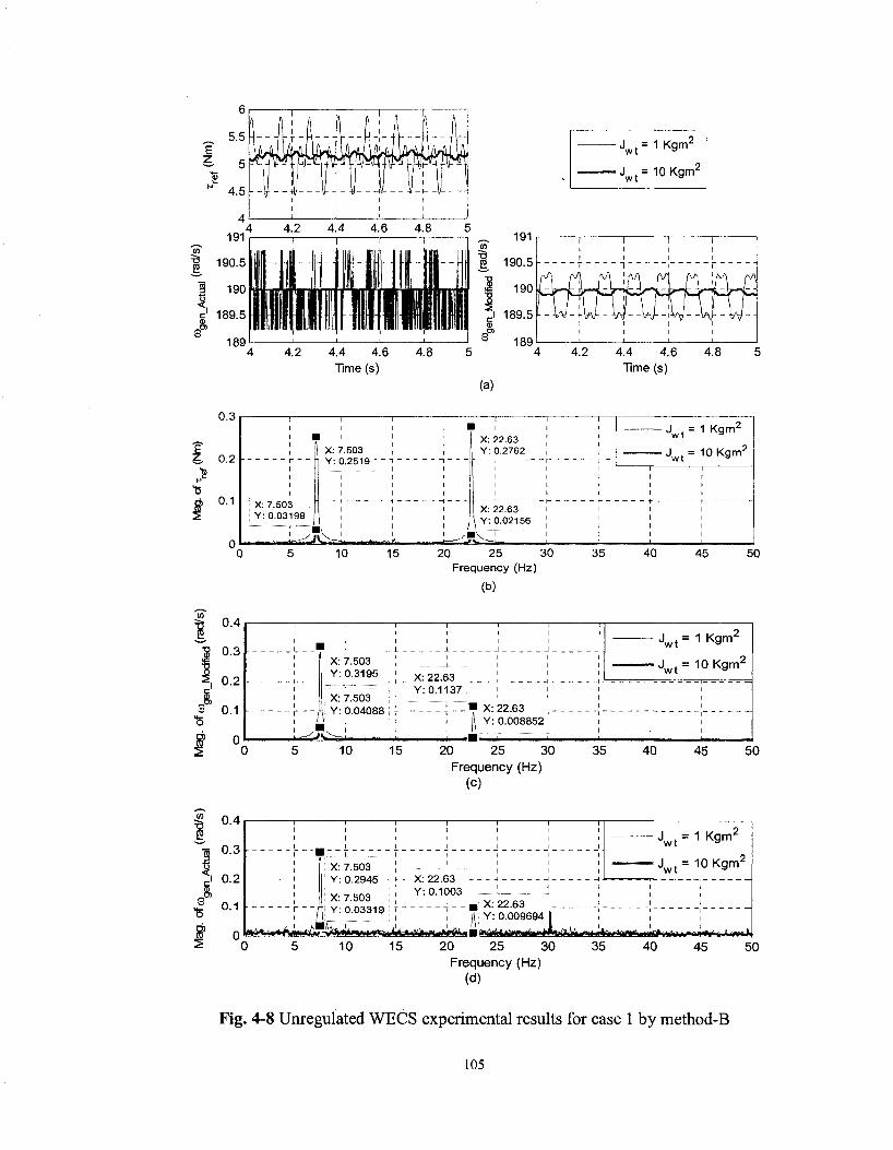
189 4.2
J w t = 1 K g m 2
• J w , = 10Kgm2
mwomr 4.4 4.6
Time (s) 4.8
0.3
0.2
0.1
I 1
r
"" X: 7.503 Y: 0.03199
I I I I I I I
| l I I
X: 7.503 \ | Y : 0.2519 " ^ "i
i i i
iO . [ Li
I 1 1 • 1 1 !
X: 22.63 \ ] Y : 0.2762 , ,
i i r
- i t — X: 22.63 i i
\ Y : 0.02156 ] |
i v ' ' '
J w t = 1 K g m 2
J w t = 1 0 K g m 2
X I I
10 15 20 25 30 Frequency (Hz)
(b)
35 40 45 50
0.4
0.3
0.2
0.1
0 0
X: 7.503 Y: 0.3195
X: 7.503 Y: 0.04088
l_ X: 22.63 Y: 0.1137
X: 22.63 Y: 0.008852
10 15 20 25 30 Frequency (Hz)
(c)
35
"wt 1 Kgrrr
• J w t = 1 0 K g m '
40 45 50
0.4
0.3
0.2
0.1
X: 7.503 Y: 0.2945 - •<- - X: 22.63
-t\ X: 7.503 Y: 0.03319
Y: 0.1003 X: 22.63 Y: 0.009694
0 mib*u**4vi»*L* -i?SWi»w«n»<aM.4fc» ̂ MttoUmttU • *^LkLMt^**j:l&Jm*n* 1
- J w t = 1 K g m 2
. J w t = 1 0 K g m 2
lh-l |W»ii<J»,-i^M*|i ' a.tw<ii 10 15 20 25 30
Frequency (Hz) (d)
35 40 45 50
Fig. 4-8 Unregulated WECS experimental results for case 1 by method-B
105
There are some discrepancies between the magnitudes of the oscillatory torque
components of method-A and method-B which are mainly due to generator speed signals
which normally present non-zero values for all frequencies, for instance, about 0.02 rad/s
as it can be seen on the generator speed frequency spectrum. This causes an error of 10%
in some cases, since the values of variations on the generator speed are relatively very
small and the values of noise or disturbance are to them. Thus, they contribute in creating
the components of the reference torque which causes an error between the two methods.
According to equation 2-14, the system natural frequencies for Jwt equal to 1 and
10 kgm2 are 14.1 and 12.65 Hz, respectively. Now, by referring to Fig. 4-7, additional
components on the reference torque can be observed for both wind turbines with Jwt equal
to 1 and 10 kgm2. The frequencies of these components are close to the systems' natural
frequencies. This usually happens because the generator speed signal presents non-zero
values for the frequencies around the system's natural frequency which creates additional
component on the reference torque.
These frequencies are highly attenuated by applying method-B as it can be seen in
the frequency spectra of reference torque and the generator modified speed in Fig. 4-8.
The reason is that the actually modified generator speed signal has been fed back to the
model of the wind turbine which presents a more ideal speed signal than the actual
measured generator speed signal.
Case 2) In this case the effect of the wind turbine with masses moment of inertias
equal to 1 and 10 kgm2 on suppressing the system responses variations due to the wind
speed variations are investigated. The results for this case are shown in Fig. 4-9 (by
106
applying method-A) and Fig. 4-10 (by applying method-B). The wind speed profile for
this case is Vw = 7.87 + 0.2 sinlitt + 0.2 sin6iti + 0.2 sinXhct m/s. It should be noted that
the wind speed profile for wind turbines with Jwt equal to 1 and 10 kgm2 are not in phase
since the results for two cases are captured at different time. The results are taken in
steady-state. The oscillatory torque components are set to zero, thus the variations on the
system responses are due to wind speed harmonics only. The results show that the effect
of variations on the reference torque and the generator speed are less for the case where
the wind turbine has higher mass moment of inertia.
The relation between the generator speed, input (reference) torque, and generator
torque (load torque plus the torque due to the generator losses) for the prime mover and
the generator as one mass can be calculated (in frequency domain) by the well-known
equation 4-3.
£l{j2nf) = - ^ — g — (4-3) jln/Jj+BT
Where Q is the generator speed in rad/s, Tref is the applied torque to the generator in Nm,
Tgen is the load torque plus the torque due to the generator losses in Nm,/ is the complex
number equal toV-1 , / i s the frequency of the applied torque in Hz, JT and Br are the sum
of masses moment of inertias in kgm2 and sum of friction constants in Nms/rad of the
prime mover and the generator which are equal to 0.0174 and 0.00245, respectively.
Thus, the magnitudes of the generator torques and speed ignoring the effect of Br, which
has high effect for the frequency range very close to zero, can be related as:
P(j27Tf)\ « TrefU2nf)-TgenU2nf)
InfJj (4-4)
107
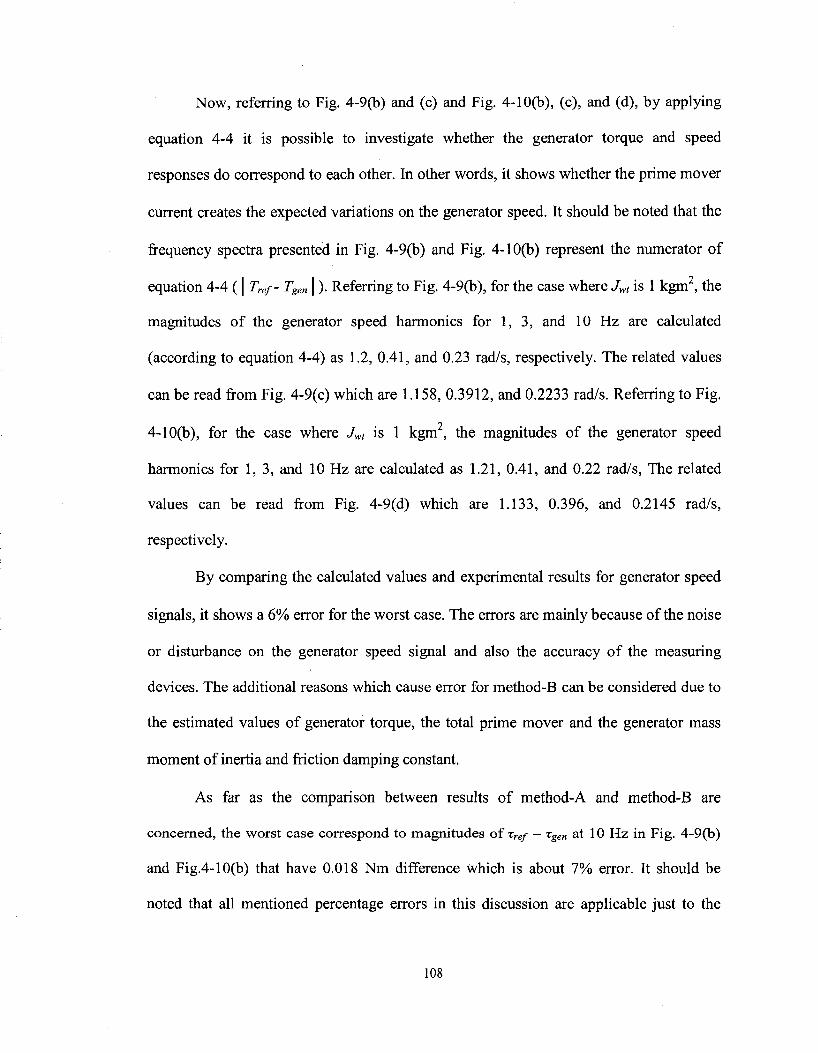
Now, referring to Fig. 4-9(b) and (c) and Fig. 4-10(b), (c), and (d), by applying
equation 4-4 it is possible to investigate whether the generator torque and speed
responses do correspond to each other. In other words, it shows whether the prime mover
current creates the expected variations on the generator speed. It should be noted that the
frequency spectra presented in Fig. 4-9(b) and Fig. 4-10(b) represent the numerator of
I I 9
Tref- Tgen \ ). Referring to Fig. 4-9(b), for the case where Jwt is 1 kgm , the
magnitudes of the generator speed harmonics for 1, 3, and 10 Hz are calculated
(according to equation 4-4) as 1.2, 0.41, and 0.23 rad/s, respectively. The related values
can be read from Fig. 4-9(c) which are 1.158, 0.3912, and 0.2233 rad/s. Referring to Fig.
4-10(b), for the case where Jwt is 1 kgm , the magnitudes of the generator speed
harmonics for 1, 3, and 10 Hz are calculated as 1.21, 0.41, and 0.22 rad/s, The related
values can be read from Fig. 4-9(d) which are 1.133, 0.396, and 0.2145 rad/s,
respectively.
By comparing the calculated values and experimental results for generator speed
signals, it shows a 6% error for the worst case. The errors are mainly because of the noise
or disturbance on the generator speed signal and also the accuracy of the measuring
devices. The additional reasons which cause error for method-B can be considered due to
the estimated values of generator torque, the total prime mover and the generator mass
moment of inertia and friction damping constant.
As far as the comparison between results of method-A and method-B are
concerned, the worst case correspond to magnitudes of zref — rgen at 10 Hz in Fig. 4-9(b)
and Fig.4-10(b) that have 0.018 Nm difference which is about 7% error. It should be
noted that all mentioned percentage errors in this discussion are applicable just to the
108
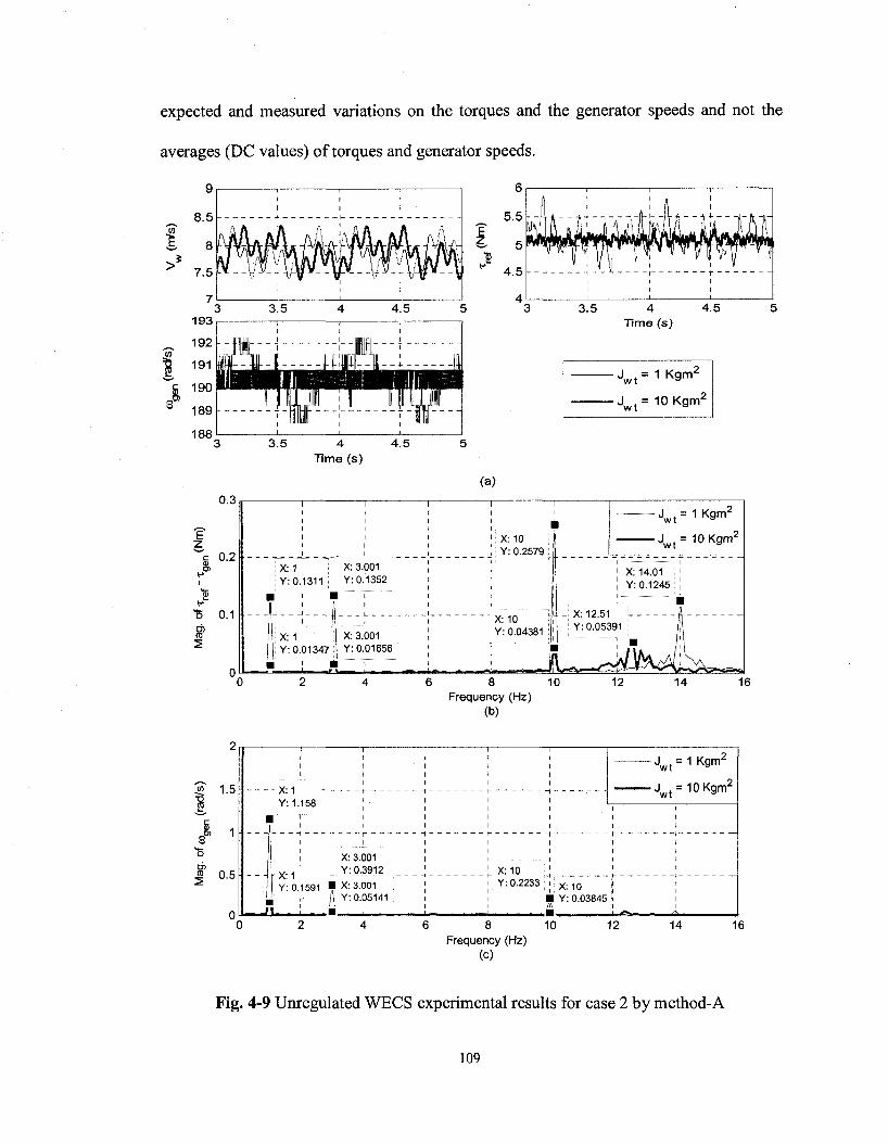
expected and measured variations on the torques and the generator speeds and not the
averages (DC values) of torques and generator speeds.
!
>s
f 1 8
9
8.5
8
7.5
7
193
192
191
190
189
188
I ! I I I I
A f t 'ft A ' A ft 'ft A
1 TiAv \ ITA lA I A\A\ r I lAvYfnVAA 7 A\M"
i i i i i i
0.3
0.2
"5 0.1 TO 2
3 .5 4 . 5
J w t = 1 K 9 m
• J w t = 1 0 K g m 2
(a)
X: 1 X: 3.001 Y: 0.1311 : Y: 0.1352
X: 3.001 Y: 0.01656
- J w t = 1 K g m '
• J w ( = 1 0 K g m 2
X: 14.01 Y: 0.1245
H-; X: 12.51 Y: 0.05391
i i ilun < niiwni-i f | \ -"S**~>£^-~y*-6 8 10
Frequency (Hz) (b)
12 14 16
« 1.5
S "S di « 0.5
X:1 Y: 1.158
X:1 Y: 0.1591
X: 3.001 . Y: 0.3912 X: 3.001 Y: 0.05141
X:10 Y: 0.2233 : X:10
Y: 0.03845
10 12 Frequency (Hz)
(c)
J w t = 1 K g m '
• J w t = 1 0 K g m 2
14 16
Fig. 4-9 Unregulated WECS experimental results for case 2 by method-A
109
9
8.5
8
7.5
7 193
192
191
190
189
188
I I I
I I I
I I I
3 3 .5 4 4 . 5 5 1 f I
3.5 4 Time (s)
4.5
J w t = 1 Kgm' J w t = 10 Kgm
0.3 E z
I 0-2
£ 0.1
2
5 1-2 6 1
I °-8
2, 0.6
S "S en (0
5
.a o.4 0.2
0
«• 1.2
JS 1
I 0.8
c1 0.6 \
S01 0.4 'o
en
2
0.2
X:1 Y: 0.1327
X: 3.001 Y: 0.1361
X: 1 | X: 3.001 Y: 0.01706 : Y: 0.01555
. X:10 Y: 0.2399
X:10 ! Y: 0.03885
.JflL. 6 8 10
Frequency (Hz) (b)
_ . '
u
X' 1 i -l ' Y: 1.156 ! !
' X: 3.001 i !" " Y: 0.3987 " "J
X: 1 • ' Y: 0.1434 II X: 3.001 j
\ i • ;
i
i
X: 10 : ' • Y' 0 2212 " I "
I X:10 " • Y: 0.0355
•
J w t = 1 K g m 2
J w t = 1 0 K g m 2
I I
I
6 8 10 Frequency (Hz)
(c)
12 14 16
1
" •
. . .
u
i ! i ! X: 1 | | Y: 1.133 ' i
! [ X: 3.001 1 Y: 0.396 i
: X: 1 • Y: 0.1529 II X: 3.001
1 1 i
1
• X: 10 ' 1 Y: 0.2145 : [~
! X: 10 ' f Y: 0.0208:
J w t = 1 K g m 2
J w t = 1 0 K g m 2
t I
' '
r -i
8 Frequency (Hz)
(d)
10 12 14 16
Fig. 4-10 Unregulated WECS experimental results for case 2 by method-B
110
Case 3) In this case the excitation of the system's natural frequency is
investigated. The results for this case are shown in Fig. 4-11(a) and (b) (by applying
method-A) and Fig. 4-11(c) (by applying method-B). The wind speed profile for these
tests is Vw = 7.87 + 0.4 sin267rt m/s. The natural frequency of the system is 13.04 Hz.
The results in both figures are captured in steady-state condition except for Fig. 4-11(a)
which is explained below. First, comparison between the two methods is discussed.
In Fig. 4-11(a) the implementation with method-A is shown. The shaft damping
constant (Bsh), as given in Table 4-2, is set equal to 0.7307 Nms/rad. At the time when the
13 Hz harmonic is added to the wind speed, the reference torque started to grow
unbounded, for this reason the 13 Hz component from the wind speed has been set to
zero which caused a reduction in the reference torque to its steady-state value as shown in
the figure. The same test by method-B was done as shown in Fig. 4-11(c) where Bsf, is
equal to 0.7307 Nms/rad. The variation on the reference torque is quite large but it is
bounded and was not growing. It can be concluded that the effect of values of Bsh on
implementation by method-A are not as effective as they should be (this matter is
discussed in the tests presented in the following cases as well).
The results of Fig. 4-11(b) show the system responses by method-A where BSh is
set equal to 2 Nms/rad. As a result, the reference torque was bounded and the results are
very close to the results by method-B with Bsh = 0.7037 Nms/rad. By these tests it can be
concluded that since the frequency of the wind speed harmonic, 13 Hz, is very close to
the system's natural frequency the variations on the reference torque is high. The actual
and modified generator speed signals in the results by method-B are provided for
comparison purpose which shows how close these two signals are.
i l l
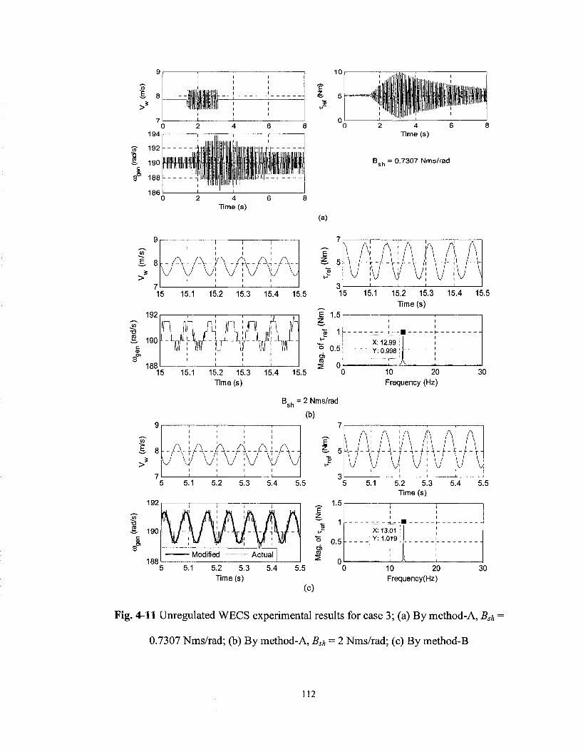
I 8 ^ 5
192
•3
& 190
188 15
192
Bo. = 0.7307 Nms/rad sn
(a)
15.2 15.3 15.4 15.5 15.1 15.2 15.3 15.4 15.5 Time (s)
15.1 15.2 15.3 15.4 15.5 Time (s)
10 20 Frequency (Hz)
30
B„u. = 2 Nms/rad "sh
(b)
£ 5
5.1 5.2 5.3 5.4 5.5 5.1 5.2 5.3 5.4 5.5 Time (s)
E z
2
1.5
0.5
- - - . . H - - I X: 13.01 I
i Y: 1.019:
; I 1 '
5.2 5.3 Time (s)
(c)
10 20 Frequency(Hz)
30
Fig. 4-11 Unregulated WECS experimental results for case 3; (a) By method-A, BSf,
0.7307 Nms/rad; (b) By method-A, Bsh = 2 Nms/rad; (c) By method-B
112

Case 4) In this case it is investigated how the 3 harmonic of the oscillatory can
excite the system's natural frequency. The results for this case are shown in Fig. 4-12(a)
(using method-A) and Fig. 4-12(b) (using method-B). In this case the shaft torsional
spring constant (Ksh) is set equal to 4500 Nm/rad. Therefore, according to equations 2-14
and 2-18, the system's natural frequency and shaft damping constant (Bsh) are calculated
as 21.15 Hz and 1.185 Nms/rad, respectively. As it was mentioned in the case 1, for rated
generator speed the frequency of 3rd harmonic of the oscillatory torque is 22.68 Hz. Since
this frequency is close to the system's natural frequency; as it can be seen from the Fig.
4-12 high variations on the reference torque should be expected due to the 3rd harmonic
of the oscillatory torque. The frequency spectrum of the reference torque in Fig. 4-12(a)
shows a component at 20.95 Hz which is very close to 21.15 Hz (system's natural
frequency) but, this component is eliminated by applying method-B. It should be noted
that the 20.95 Hz component should not be appeared on the reference torque response.
The reason is that the reference torque variations are due to wind turbine oscillatory
torque only. Thus the components with the frequencies about 7.5 Hz (1st harmonic) and
22.7 Hz (3r harmonic) must exist.
It should be noted that the value of BSh for the implementation by method-A was
3.2 Nms/rad; the minimum value which allowed the system to operate otherwise the
reference torque would grow boundlessly. There was no such limitation for
implementation by method-B. So, the results by method-B are provided for Bsh = 1.185
Nms/rad.
113
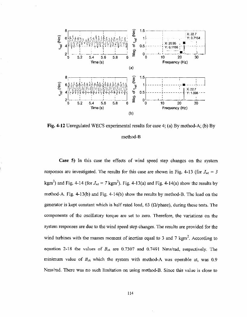
z
o> 4
"8 4
5.4 5.6 Time (s)
8>
1.5
1
0.5
0
(a)
X: 22.7 Y: 0.7154;
X: 20.95 Y: 0.1155
10 20 Frequency (Hz)
30
1 I I
••- „„m.™X,n>k-««-
X: 22.7 Y: 1.008 - - -
f S r-U r
10 20 Frequency (Hz)
30
Fig. 4-12 Unregulated WECS experimental results for case 4; (a) By method-A; (b) By
method-B
Case 5) In this case the effects of wind speed step changes on the system
responses are investigated. The results for this case are shown in Fig. 4-13 (for Jwt = 3
kgm2) and Fig. 4-14 (for Jm = 7 kgm2). Fig. 4-13(a) and Fig. 4-14(a) show the results by
method-A. Fig. 4-13(b) and Fig. 4-14(b) show the results by method-B. The load on the
generator is kept constant which is half rated load, 63 (£J/phase), during these tests. The
components of the oscillatory torque are set to zero. Therefore, the variations on the
system responses are due to the wind speed step changes. The results are provided for the
wind turbines with the masses moment of inertias equal to 3 and 7 kgm2. According to
equation 2-18 the values of Bsh are 0.7307 and 0.7491 Nms/rad, respectively. The
minimum value of Bsh which the system with method-A was operable at, was 0.9
Nms/rad. There was no such limitation on using method-B. Since this value is close to
114

the values calculated above, all the tests for method-A and method-B are done for Bsh -
0.9 Nms/rad.
The wind speed is kept constant at 7.87 m/s. Then, step changes of ±1 m/s are
applied to the wind speed as shown in the figures. By comparing the results of Fig. 4-13
and Fig. 4-14, it can be clearly seen that the transient response of the system with the
wind turbine with higher mass moment of inertia is slower. The other point is that with
each step change in the wind speed the system's natural frequency will appear on the
reference torque before it reaches its steady-state. These are shown in Fig. 4-13 (a) and
(b). The system's natural frequency when Jwt = 3 kgm2 is 13.04 Hz. The calculated
frequencies (based on the points marked on the zoom of the reference torques, bottom-
right figures of Fig. 4-13(a) and (b)) for method-A is 12.97 Hz and for method-B is 13.07
Hz which are very close to the theoretical value with an error of less than 0.5%.
The generator phase voltage waveform is shown in Fig. 4-14(a). It can be seen
that with each wind speed change, the generator voltage varies significantly (about 25%
in this case) which shows the necessity of regulating the WECS.
The reference current and prime mover current waveforms are provided in each
figure to show their transients. In Fig. 4-14(b) the modified and actual generator speed
signals are indicated showing that the modified speed signal has the same transient
response as the actual speed with much less noise or disturbance. It can be also seen that
the implementation by method-B presents the same transient as the implementation by
method-A does.
115

r 8
5 7 IZ 10 20
10 20 Time (s)
5 7
10 20
^ 4
=§ 195
| 185 3, & 175
10 20
30
30
30
10 20 Time (s)
30
10 20 30
1 5 1 ' ZbOm1 Of T ,' V. /I Q7C
i . / i \J\ A i Y: 4.464
_J 1 I L_ w 4 4.2 4.4 4.6 4.8 5
Time (s) (a)
crx::::! I 4
10 20 30
IT \ ?!
e 4
2
5.5
I 5
%/*v •
10 20 30
Zoom of x ref
X: 4.216 1 4.5 M Y : 5.031
X: 4.675 . Y:4.49
4 4.2 4.4 4.6 4.8 5 Time (s)
(b)
Fig. 4-13 Unregulated WECS experimental results for case 5 (Jwt = 3 kgm2); (a) By
method-A; (b) By method-B
116
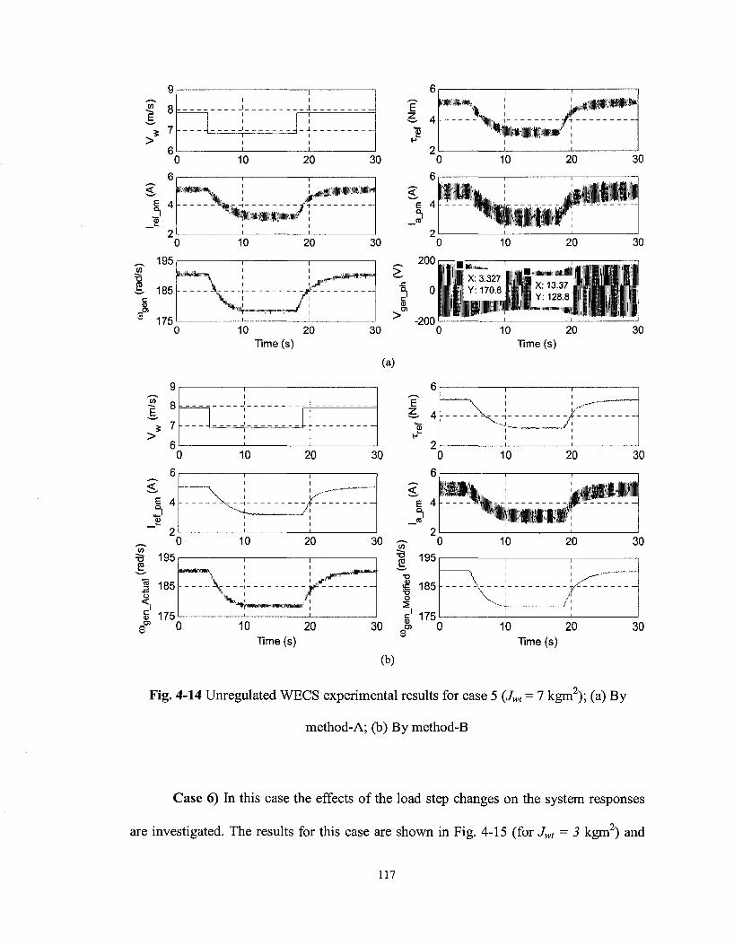
9
? 8
% 7
i4
_ 195
1 185
175
^ 4
1 2
_ 0
x> 195 -£
§ 185
S 175
I I
0 10 20 30
0 10 20 30
. . . . .V_. j *?^____J \ j /j
10 20 Time (s)
30 10 20 Time (s)
(a)
J.
E S. 4 ZX.i ;.::"__.
^J_ / 10 20 30 10 20
I I
10 20 Time (s)
30
1 185 o
g 175 ra 0 10 20
Time (s)
(b)
30
30
Fig. 4-14 Unregulated WECS experimental results for case 5 (Jwt = 7 kgm2); (a) By
method-A; (b) By method-B
Case 6) In this case the effects of the load step changes on the system responses
are investigated. The results for this case are shown in Fig. 4-15 (for Jwt = 3 kgm2) and
117
Fig. 4-16(for Jwt = 7 kgm2). Fig. 4-15(a) and Fig. 4-16(a) indicate the results by method-
A. Fig. 4-15(b) and Fig. 4-16(b) indicate the results by method-B. The wind speed is kept
constant at 7.87 m/s. The components of the oscillatory torque are set to zero. Therefore,
the variations on the system responses are due to the load step changes. The results are
provided for the wind turbines with the masses moment of inertias equal to 3 and 7 kgm .
The shaft damping constant Bsh = 0.9 Nms/rad was used for all the tests in this case for
the same reason explained in case-5.
The resistive load values before and after the load disturbances are shown on the
reference torques related to each test. The systems' natural frequencies for the wind
turbines with the masses moment of inertias 3 and 7 kgm2 are 13.04 and 12.72 Hz,
respectively. By referring to figures which are zooms of the reference torques, the natural
frequencies for the systems with Jwt equal to 3 and 7 kgm2 are 13 and 12.8 Hz,
respectively, for the results by method-A. Those frequencies are calculated as 13.11 and
12.8 Hz, respectively, for the results by method-B. These values are very close to the
theoretical values presenting an error of 0.6% in the worst case.
The results show that the transient response of the system with higher mass
moment of inertia is slower. In the implementation by method-A, the shaft damping BSf, is
not as effective as it should be, as it can be clearly seen from the results. In normal
conditions before and after load disturbances (in its steady-state) there are still signs of
excitation of the natural frequency. Also it takes much longer time for the reference
torque to damp out in method-A than in method-B. The reason is because of the modified
generator speed signals in method-B which have less noise or disturbance comparing to
the generator speed signal in method-A. Referring to the results by method-B, it can be
118
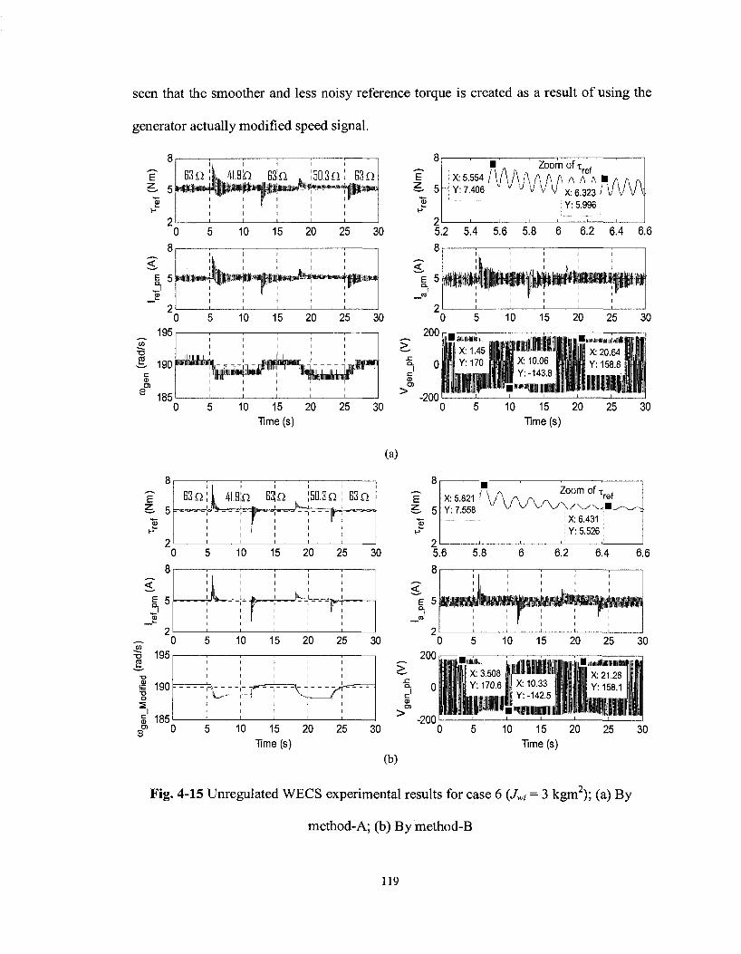
seen that the smoother and less noisy reference torque is created as a result of using the
generator actually modified speed signal.
8 r , , , , • , 8
6- 5 5D.3Q! 63 fi
185 10 15 20 25
Time (s)
rV*^+%w^-' 30
E 5- 5
p
X: 5.554 / Y: 7.406
Zoom of xref
X: 1.45 I I Y: 170 | | j
-200t
illY: 170111X: 1 0 ' 0 6 1 1 1 1 Y' 158 8
10 15 20 25 Time (s)
30
(a)
e . 5
E 5 . I
50.3 fi
10 15 20 Time (s)
63 n
10 15 20 25 30
i : i i i — s - * * — ! — » — | — ^ ^ ^ j — r j —
25 30
S 5
/1 ^ Zoom of x ,
X: 6.431 Y: 5.526
~~.
5.6
81—
5.8
E 5
6.2 6.4 6.6
15 20 25 30
lilllll X: 10.33 Y: -142.5 " l i l l l l l l
10 15 20 Time (s)
(b)
Fig. 4-15 Unregulated WECS experimental results for case 6 (Jwt = 3 kgm2); (a) By
method-A; (b) By method-B
119
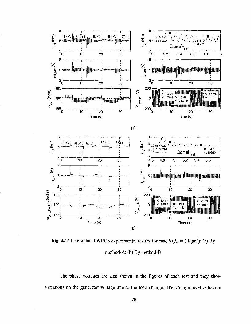
10 20 Time (s)
30
8
* 5 G3QL 4I.Bb B3n. I.3 n B3. Q
10 20 30
S5
195
190
10 20 30
I 185 3a 0 10 20
Time (s) 30
X:5.272l\[\f\f\ A A A • Y: 7.335 v V \J V X: 5.819
7 r Y: 6.261 Zoom afx f
W 5.2 5.4 5.6 5.8
X: 3.521 Y: 170.6
-200 OTB •!- • ! • • : ! ( • . i
10 20 Time (s)
30
(a)
8
1 6 $ 4
AA • . U X: 4.929 ' l / V W V V . ! Y: 6.634 ,
Zoom DTT i X: 5.476 Y: 5.659
200,
£• 1 X: 1.517 p i l m l Y i P . X 21.89 "5, o i l Y: 169.4 I X: 9.861 \.-'i Y 159.4 111 | ["FBI l | l l Y: "143-1 ijii1 *i j " n n f l
> ra i 'r' M'I '•••'lilllllll ' ' il||H ill -200' 10 20
Time (s) 30
(b)
Fig. 4-16 Unregulated WECS experimental results for case 6 (Jwt = 7 kgm2); (a) By
method-A; (b) By method-B
The phase voltages are also shown in the figures of each test and they show
variations on the generator voltage due to the load change. The voltage level reduction
120
for larger load change is about 16% and for lower load change is about 8%. The
reference current and prime mover current are provided indicating their transient and
steady-state responses.
4.4.2 R E G U L A T E D WECS
The results in this section are related to the experimental set-up shown in Fig. 4-2.
This can be considered as a stand-alone application of a regulated WECS. The top part of
Fig. 4-2, as mentioned before, was designed and implemented in [30]. The whole system
has been tested under two major cases which show the transient and steady-state
responses of the regulated WECS due to wind speed and load variations. The results are
shown for the WTE implemented with method-A and method-B. In all results the
oscillatory wind turbine torque is in effect.
There was a limitation on using method-A. The system response was unstable
(reference torque was growing) for the shaft damping constant (Bsh) less than 2 Nms/rad.
Therefore, all results for method-A are taken with BSh equal to 2 Nms/rad. Since, there
was no limitation for the implementation with method-B, the results for this method, are
taken for the shaft damping constant (Bsh) equal to 0.7307 Nms/rad when Jwt = 3 kgm
and 0.7419 Nms/rad when Jwt = 7 kgm2. These values are calculated according to
equation 2-18.
Case 1) The effects of wind speed step changes are investigated in this case for
the wind turbine with the mass moment of inertia 3 and 7 kgm2. The results for this case
are shown in Fig. 4-17 and Fig. 4-18. Fig. 4-17 indicates the results for the wind turbine
121
with the mass moment of inertia 3 kgm2 and Fig. 2-18 indicates the results for the wind
turbine with the mass moment of inertia 7 kgm2. In each figure the results are provided
for the implementation with method-A and method-B. Step changes of 1 m/s are applied
on the wind speed of 7.9 and 6.9 m/s to observe the system responses due to these
changes. As it can be seen from the results of both figures, as wind speed decreases the
VSI supplies some portions of active power required for the fixed load, 63 £J/phase, in
order to maintain the generator speed close to its rated speed.
In other words, the generator sees smaller load even though the load connected to
its output is kept unchanged. It should be noted that the generator speed when wind speed
is equal to 6.9 m/s is slightly lower than the time when wind speed is equal to 7.9 m/s.
This is acceptable, because the aim is to regulate the frequency of the generated voltage
and not the shaft speed. Recall that there is the slip factor for induction
machines/generators. So as the generated power decreases, the shaft speed required for
producing power/voltage with a given frequency decreases.
By comparing the results of the Fig. 4-17 and Fig. 4-18, it can be concluded that
the responses for the wind turbine with mass moment of inertia Jwt — 3 kgm2 has more
oscillations to reach to its steady-state than the case where the wind turbine has the mass
moment of inertia Jwt = 7 kgm2. It can be also concluded that the implementations by
method-A and method-B result in very close responses with the fact that there is no
limitation on setting the value of the shaft damping (Bsh) for the implementation with
method-B.
122
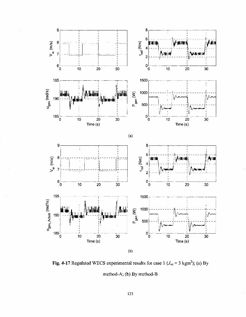
1
•3 2
"» 8
10 20
10 20 Time (s)
30
8
_ 6
E
X 4
H 2
0
1500
1000
a? 500
(a)
I 1 I
I ! I
8
_ 6 If £. 4
10 20
10 20 Time (s)
30
iT^ET F 30
I ! I i I i
my j km^ \K^U i
! I 1 1
Mpi
r T^j|P'"W^'"'»'H"*IHl'('*^ I
V - - - , - - -
10 20 30 10 20 30
195 in
•o S
| 190
TO
185 10 20
Time(s) 30
(b)
10 20 Time (s)
Fig. 4-17 Regulated WECS experimental results for case l(JM = 3kgm2);(a)By
method-A; (b) By method-B
123
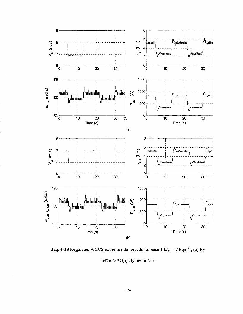
"Tn 8
1-> 5 7 — 1 - - 1 1 ,
10 20 30
•6
185
JO O
r* 7
10 20 Time (s)
1500
1000
c
a.& 500
30 35
(a)
I I t
5TF5IE
10 20 30
8
_ 6
£ 4 to
P 2
0
10 20 Time (s)
30
T K 1
10 20 30
(3
3 190 £
10 20 Time (s)
1500
g- 1000
c
n & 500
(b)
10 20 Time (s)
Fig. 4-18 Regulated WECS experimental results for case 1 (Jwl = 7 kgm2); (a) By
method-A; (b) By method-B.
124

It is worth mentioning that the value of Bsh is mainly very effective on the
system's natural frequency and frequencies close to it. By comparing the reference torque
responses obtained by method-A and method-B, it can be seen that the response by
method-A is noisier than the response by method-B even though the shaft damping was
set to a higher value in method-A. The value of BSf, does not affect the transient time and
general shape of the responses in transition from one state to another. But, in method-A
the oscillations with the system's natural frequency around the average values in steady-
state and transient are less damped even for larger value of Bsh-
Case 2) The effect of the load variations are investigated in this case for the wind
turbines with the masses moment of inertias 3 and 7 kgm2. The results for this case are
shown in Fig. 4-19 and Fig. 4-20. The wind speed is kept constant at 7.9 m/s for these
tests. Fig. 4-21 shows the results for the wind turbine with the mass moment of inertia 3
kgm2 and Fig. 2-20 shows the results for the wind turbine with the mass moment of
inertia 7 kgm2. In each figure the results are provided for the implementation with
method-A and method-B. The resistive loads have been changed as their values are
shown on the reference torques responses of each figure before and after the load change.
It should be noted that the values of the resistances are phase values.
The results show that since the wind speed is constant the VSI operates in such a
way that the generator sees constant load which is 63 (Q/phase). In other words, the
reference torque, the generator speed, and the generator power remain the same in steady-
State after each load change. The generator phase voltage is also provided and shows that
it remains constant before and after each disturbance. The number of oscillations on the
125
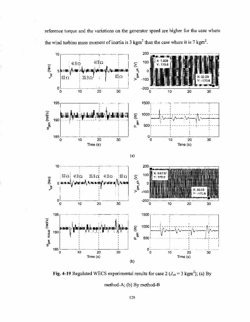
reference torque and the variations on the generator speed are higher for the case where
the wind turbine mass moment of inertia is 3 kgm2 than the case where it is 7 kgm .
10 | , , , , 200 r
100 h i * 1 928 h j f , | l|| Y 170 6 |l|,l |'
> -100
-200 L M'Y
P mm *\ °tl||l
I ill,' \ \ I ' l l I'll"' '\ I" X 32 29 ' l '
I lift1 Vl I'l'f.l'fV "" H 10 20 30
195
in
& 190 c <D
J3>
185
10
E £ 5 H1"
63 Q
1 1 1 1 1 1 1
1 ' 1 If
! 1
10 20 Time (s)
30
1500
g- 1000
c
Q.ra 500
0
i " i | i a. i J i.
(a)
1 n f , .I X 3 73 4l.9h 35.Bfi! 4I.BQ |B3« g 1 0 ° ' Y 17( b I
r J ° Hi i
200-
10 20 Time (s)
30
i' it'll •it iji
Oi
10 20 30 -200L
|yiHPi,iy 70 111
10 20 30
195 in
&
| 190
185 10 20
Time (s)
*--• - T - - T "-x - ' - I - •"- j r - —
30
1500
1000
D.01 500 i i • i
(b)
10 20 Time (s)
30
Fig. 4-19 Regulated WECS experimental results for case 2 {Jm = 3 kgm2); (a) By
method-A; (b) By method-B
126
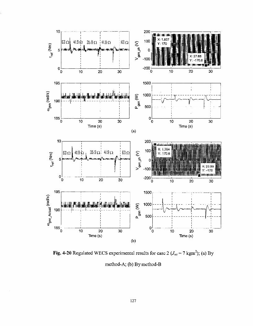
200
— 100 1, 1 8 3 7 ,1|
°l
> -100
II Y 1 7 ° |Mf j y'Hi i
X 27 68 Y 170 6
-200 l
10 20
iV. 30
I I I I
_ i _ _ _ : _ . J
—\P—^v~-—^J^^^-JX^
\ i
10 20 Time (s)
(a)
10 20 Time (s)
30
200 r
100 X 1 764 Y 170 6
I. JJll
i.W »f --\wmw^h -200 L
10 20 30
195
10 20 Time (s)
30 10 20 Time (s)
30
(b)
Fig. 4-20 Regulated WECS experimental results for case 2 (Jwt = 7 kgm2); (a) By
method-A; (b) By method-B
127
4.5 CONCLUSIONS
The 2-hp WTE designed and implemented in Chapter 3 was used for emulating a
stand-alone WECS by replacing the dynamometer with a self-excited induction
generator. The new configuration provided the opportunity as a test bench to first, test the
unregulated WECS and investigate the effect of wind speed variations, load variation,
and system parameters on the generator behavior and produced electricity. Then, the
designed WTE was used in a stand-alone regulated WECS which can be counted as one
of real application of the designed WTE. The part of the system which was controlling
and regulating the generator voltage and frequency was designed and implemented by
Mr. Ghulam Dastagir who was M.A.Sc. Student in the Electrical Engineering
Department.
The WTE has been implemented with two methods called method-A and method-
B. They are both effective but have disadvantages. The main disadvantage of method-A
is that in some cases it does not work (instability occurs) if the value of Bsh is set below a
certain value. This minimum value changes from case to case. In other words, the value
of Bsh cannot be varied as widely as it should for practical applications.
The main disadvantages of implementation by method-B is that the filter's corner
frequencies might need to be changed for wind turbines with different natural
frequencies; in order to attenuate those frequencies from generator speed signal. It also
requires the estimation of the total mass moment of inertia friction constant of the prime
mover and the generator and also the generator torque. To estimate the generator torque,
the generator power needs to be measured which requires additional current and voltage
sensors in comparison with method-A.
128

The main features of the designed and implemented WTE are:
> Capable of emulating the wind turbines with different mass moment of
inertias, drive train with flexible shaft with different torsional spring
constants, and damping constants, and ideal gear box with different gear
ratios.
> Capable of emulating the oscillatory torque.
> Provides the capability of experimentally verifying the facts highlighted in
conclusion of Chapter 2 as simulation results.
129
CHAPTER 5
CONCLUSIONS
5.1 SUMMARY
The increased level of penetration of wind power in the power generation systems
has motivated a further analysis of the dynamic behavior of the wind energy conversion
systems (WECS). A key element in a WECS test bench is a wind turbine emulator
(WTE) which can be described as a controllable source of mechanical torque with the
features of a wind turbine (rotor) and drive train. Different ways of implementing WTEs
have been proposed in the literature. They can be categorized in terms of complexity of
the wind turbine model, type of the electric machine as prime mover, number of feedback
signals such as torque and speed signals, types of power electronics converters, and
control strategies.
In this Thesis, a simplified model of a wind turbine consisting of the wind turbine
mass moment of inertia and damping constant, a flexible low speed side shaft with
damping constant, an ideal gear box, a rigid high speed side shaft, and the generator with
the mass moment of inertia and damping constant. This simple configuration provides the
opportunity for investigating the effects of four important factors on the system responses
which are the mass moment of inertia, the system's natural frequency, the shaft damping
constant, and the oscillatory torque.
A 2-hp WTE was designed and implemented to investigate whether the expected
results can be achieved experimentally. In the first step, the WTE has been preliminary
tested by using a dynamometer as mechanical load. Using the dynamometer eliminates
130
the requirement for having electrical generator and load, since it works as a variable
mechanical load. The desired torque for the wind turbine emulator and dynamometer can
be defined as a function in the MATLAB/Simulink model, for simulation studies and
later for practical implementation using the dSPACE ds-1103 DSP development kit. The
experimental set-up performed well and the experimental results presented good
correlation with the simulation results.
The same 2-hp WTE with slight modifications (to be suitable for applying it to
WECSs) was used for running a self-excited induction generator in the unregulated and
also in the regulated stand-alone mode. The WTE was implemented by two methods of
measured speed signals which are called method-A (using actual speed signal) and
method-B (using a modified speed signal). Several tests were carried out by both
methods. Implementation by method-A was limited by a minimum value of the shaft
damping constant. There was no such limitation for implementation by method-B, but in
this method, the transfer functions of the filters might need to be changed for different
wind turbines. It was shown that the transient and steady-state responses for both
methods agree with each other except for the cases where the system's natural frequency
is excited; in these cases, for implementation by method-A, the shaft damping constants
had to be set to higher values than the theoretical values to prevent system's instability.
In the end, it can be stated that the implemented WTE is effective (with some
limitations) in providing the expected results on the high speed shaft responses due to
four important characteristics of the wind turbine which are the mass moment of inertia,
the system's natural frequency, the shaft damping constant, and the oscillatory torque.
The implemented WTE, in its actual form, is suitable to be used in a test bench for
131

investigating the performances of different control strategies as part of WECS which
might be proposed in the future.
5.2 SUGGESTIONS FOR FUTURE WORK
(1) Improving the capability of the WTE by:
> Using an incremental encoder with higher number of pulses/revolution, in this
case implementation by method-A should have less limitation on the value of
the shaft damping constant.
> Using higher version of MATLAB/Simulink and dSPACE which will make
the data transmission to be done at lower sampling time. In this case, the
reactance of the inductor in series with the prime mover can be reduced which
results in capability of emulating higher rate of change of prime mover torque.
> Using additional current and voltage sensors for each phase of the generator.
In this case, it is possible to measure the power of the generator for
unbalanced loads, which is necessary for implementation of the system by
method-B.
(2) Development of the hysteresis current controlleds) in such a way to be able to use
the generator or the dynamometer for the start up of the wind turbine and enforcement of
the prime mover to act as load (wind turbine rotor resistance against rotation) in this
situation. Since it is mentioned in the literature that in some WECSs the generator is also
used for start-up of the wind turbine.
132

(3) Testing the WTE in a grid connected configuration. This provides the opportunity
to investigate the excitation of the system's natural frequency (equation 2-15), since
excitation of this mode occurs on a condition that the generator speed is constant.
133
REFERENCES
[1] National Renewable Energy Laboratory (NREL), "http://www.nrel.gov/".
[2] Wind Service Holland, Member of "World Wind Energy Association",
"http://home.wxs.nl/~windsh/wsh.html".
[3] E. Hau, "Wind Turbines: Fundamentals, Technologies, Application, Economics",
Springer, 2nd (English) edition, 2006.
[4] A. D. Napoli, F. Crescimbini, and G. Noia, "A Microprocessor Controlled D. C.
Drive of Wind Turbines", European Wind Energy Conference and Exhibition (EWEC
89), pp. 687-691.
[5] T. Ackermann, "Wind Power in Power Systems", John Wiley and Sons Ltd., 2005
[6] L. A. C. Lopes, J. Lhuilier, A. Mukherjee, and M. F. Khokhar, "A Wind Turbine
Emulator that Represents the Dynamics of the Wind Turbine Rotor and Drive Train",
Proceedings of 36th Annual IEEE Power Electronics Specialists Conference (PESC'05),
June 2005, pp. 2092-97.
[7] M. Monfared, H. M. Kojabadi, and H. Rastegar, "Static and dynamic wind turbine
simulator using a converter controlled dc motor", Elsevier Ltd., Renewable Energy 33
(2008) 906-913, June 2007.
[8] B. Rabelo, W. Hofmann, M. Gluck, "Emulation of the Static and Dynamic Behaviour
of a Wind-turbine with a DC-Machine Drive", Proceedings of 35th Annual IEEE Power
Electronics Specialists Conference (PESC'04), June 2004, pp. 2107-12.
[10] S. H. Song, B. C. Jeong, J. H. Oh, G. Venkataramanan, H. I. Lee, and J. J. Kim,
"Emulation of Output Characteristics of Rotor Blades Using a Hardware-In-Loop Wind
134

Turbine Simulator", Proceedings of 20 Annual IEEE Applied Power Electronics
Conference and Exposition (APEC'05), March 2005, Vol. 3, pp. 1791-96.
[11] P. E. Battaiotto, R. J. Mantz, and P. F. Puleston , "A Wind Turbine Emulator Based
on A Dual DSP Processor System", Control Eng. Practice, 1996, Vol. 4, No. 9, pp. 1261-
66.
[12] R. Cardenas, R. Pena, G. M. Asher, and J. C. Clare, "Experimental emulation of
wind turbines and flywheels for wind energy applications", European Power Electronics
and Applications Conference, EPE2001, Graz, Austria, August 2001, pp. 1-10.
[13] D. Dolan, "Real-Time Wind Turbine Emulator Suitable for Power Quality and
Dynamic Control Study", A M.A.Sc. Thesis, University of Toronto, 2005.
[14] H. M. Kojabadi, L. Chang, and T. Boutot, "Development of a Novel Wind Turbine
Simulator for Wind Energy Conversion Systems Using an Inverter-Controlled Induction
Motor", IEEE Transactions on Energy Conversion, September 2004, Vol. 19, No. 3, pp.
547-552.
[15] R. Teodorescu, F. Iov, and F. Blaabjerg, "Flexible development and test system for 11
kW wind turbine", Proceedings of 34th IEEE Power Electronics Specialist Conference
(PESC03), June 2003, Vol. 1, pp. 67-72.
[16] Bergey Windpower Co., "http://bergey.com/".
[17] N. Baines and T. Way, "Development of Prognostic/Health Management (PHM)
Technologies for Wind Turbine: Final Report", Avenca Limited, November 2006.
[18] R. T. Stefani, B. Shahian, C. J. Savant, and G. Hostetter, "Design of Feedback
Control Systems", Oxford University Press, 4th edition, 2002.
[19] G. L. Johnson, "Wind Energy Systems", Prentice-Hall Inc., 1985
135
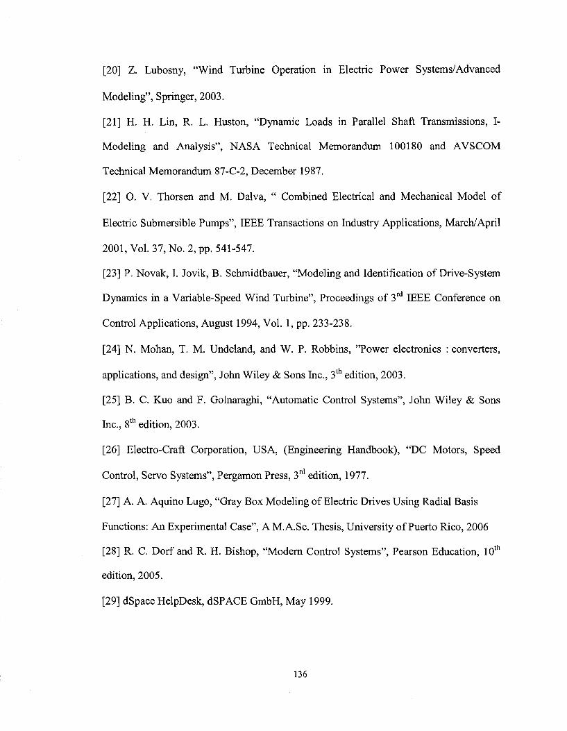
[20] Z. Lubosny, "Wind Turbine Operation in Electric Power Systems/Advanced
Modeling", Springer, 2003.
[21] H. H. Lin, R. L. Huston, "Dynamic Loads in Parallel Shaft Transmissions, I-
Modeling and Analysis", NASA Technical Memorandum 100180 and AVSCOM
Technical Memorandum 87-C-2, December 1987.
[22] O. V. Thorsen and M. Dalva, " Combined Electrical and Mechanical Model of
Electric Submersible Pumps", IEEE Transactions on Industry Applications, March/April
2001, Vol. 37, No. 2, pp. 541-547.
[23] P. Novak, I. Jovik, B. Schmidtbauer, "Modeling and Identification of Drive-System
Dynamics in a Variable-Speed Wind Turbine", Proceedings of 3rd IEEE Conference on
Control Applications, August 1994, Vol. 1, pp. 233-238.
[24] N. Mohan, T. M. Undeland, and W. P. Robbins, "Power electronics : converters,
applications, and design", John Wiley & Sons Inc., 3 edition, 2003.
[25] B. C. Kuo and F. Golnaraghi, "Automatic Control Systems", John Wiley & Sons
Inc., 8th edition, 2003.
[26] Electro-Craft Corporation, USA, (Engineering Handbook), "DC Motors, Speed
Control, Servo Systems", Pergamon Press, 3rd edition, 1977.
[27] A. A. Aquino Lugo, "Gray Box Modeling of Electric Drives Using Radial Basis
Functions: An Experimental Case", A M.A.Sc. Thesis, University of Puerto Rico, 2006
[28] R. C. Dorf and R. H. Bishop, "Modern Control Systems", Pearson Education, 10th
edition, 2005.
[29] dSpace HelpDesk, dSPACE GmbH, May 1999.
136

[30] G. Dastagir, "Voltage and Frequency Regulation of A Stand-Alone Self-Excited
Induction Generator with An Unregulated Prime Mover", A M.A.Sc Thesis, Concordia
University, Montreal, 2008
[31] M. G. Simoes and F. A. Farret, "Renewable Energy Systems: Design and Analysis
with Induction Generators", CRC Press LLC, 2004.
137

APPENDICES
APPENDIX A: RELATION BETWEEN THE WIND SPEED AND OPERATING
POINT ON THE WIND TURBINE CHARACTERISTIC
In this part it will be shown that, how the operating point can be related to the
wind speed, based on the equations introduced in Chapter 2. It can be understood easier
in the form of a question that is, for a given system parameters and specifications at what
wind speed the prime mover can generate 1500 W at the rotational speed of 188.5 rad/s
(1800 RPM). Assuming that the rotor radius is 1.7 m, the air density is 1.224 kg/m3, the
gear ratio is 4, the rotor friction constant is 0.1 Nms/rad, and Ct(X) is expressed by
equation 2-8.
In this case, the prime mover torque is equal to rpm = P/copm = 1500/188.5 = 7.96
Nm. On the other hand, the rotor speed is equal to cowt = copm/4 = 188.5/4 = 47.12 rad/s.
Now, the wind turbine must overcome the torque due to rotor losses and the high speed
side torque (the prime mover torque) considering the gear ratio. Thus, it can be written:
Twt = Bwta>wl + 4Tpm = 4.71 +31.84 = 36.55 Nm (A-l)
By equating equations 2-9 and A-l:
l/2p7rR3Ct(A)V%=36.55 => Ct{A)V^=3.S (A-2)
By combining equations 2-4, 2-8, and A-2, they can be reduced to one equation and one
unknown. The resulting equation is solved for Vw (the only unknown), by using Maple
software, and it is calculated Vw = 8.84 m/s. By using equation 2-4 and calculated wind
speed, the related tip speed ratio will be equal to 9.12. It should be noted that the tip
speed ratio at which the maximum power occurs, is 8.
138

APPENDIX B : ELECTRONICS CIRCUIT FOR SWITCHES GATING SIGNALS
Fig. B-l shows the circuit which provides the proper gating signals for the
switches in the prime mover converter leg. It provides sufficient current, required for
operating the drive circuit of the switches. It also creates the required dead time between
the gating signals for the switches, preventing short circuit. It should be noted that this
circuit was designed and built based on the suggestions provided by Mr. Yongzheng
Zhang, who was M.A.Sc. Student in the Electrical Engineering Department. The same
circuit was used for creating the dynamometer converter leg gating signals.
6.8 K« i VW 13.7 KQ
X: Prime Mover Gating Signal, from dSPACE ds-1103 Board
Y: Prime Mover Upper Switch Gating Signal, to Drive Circuit
Z: Prime Mover Lower Switch Gating Signal, to Drive Circuit
A: TL 084C/1 B: TL 084C/2 C: MC 14584B D:LM318N/1 E:LM318N/2
Fig. B-l Electronic circuit for creating gating signals for the switches
139