design and implementation of a gps receiver channel and ... · channel and multipath delay...
TRANSCRIPT

Design and Implementation of a GPS receiverchannel And Multipath Delay Estimation using
Teager-Kaiser operator.
A project report
Submitted in Partial Fulfillment of the
Requirements for the Degree of
Master of Technology
in
Computational Science
Submitted by
SABBI BABU RAO
SR NO: 5510-511-071-05309
Department of Super Computer Education and Research Centre
Indian Institute of Science
Bangalore, INDIA
June 2009

Acknowledgments
I take this opportunity to express my deep sense of gratitude to my thesis guide Prof.
S K Nandy for his constant encouragement and guidance.
I thank all the faculty members & staff of SERC for their support.
I am grateful to my parents and sister, whose faith, patience and love had always in-
spired me to walk upright in my life.
I would like to extend my heartfull thanks to my friends Adarsha,Kesavan,Mythri,
Reyaz,Bharath, Chowhan, Sainath, Sankar, Sravanthi, Prasenjit, Saptarshi, Gaurav for
making my stay at IISc a memorable one.
Special thanks to Reyaz who helped me all the way of my project for his valuable sup-
port.
S.Babu Rao
i

Contents
Acknowledgments i
List of Figures v
Abstract 1
Thesis Organization 2
1 Introduction 3
2 Position determination by Satellite Navigation 6
2.1 Position determination using PRN code . . . . . . . . . . . . . . . . . . . 6
2.2 Calculation of the User Position . . . . . . . . . . . . . . . . . . . . . . . . 10
3 GPS signal structure and characteristics 12
3.1 Modulations of GPS signal . . . . . . . . . . . . . . . . . . . . . . . . . . . 12
3.2 GPS Signal Structure . . . . . . . . . . . . . . . . . . . . . . . . . . . . . . 15
3.2.1 Frequencies,Modulation Format and PRN codes . . . . . . . . . . 15
3.3 Autocorrelation and PSD functions of random sequence of pulses . . . . 19
3.3.1 Effect of finite length PRN code on the autocorrelation function
and PSD . . . . . . . . . . . . . . . . . . . . . . . . . . . . . . . . . 21
4 GPS Receiver Channel 22
4.1 Analog front end of GPS receiver . . . . . . . . . . . . . . . . . . . . . . . 22
4.2 Digital receiver channel . . . . . . . . . . . . . . . . . . . . . . . . . . . . 24
4.3 Frequency Synthesizer . . . . . . . . . . . . . . . . . . . . . . . . . . . . . 29
ii

CONTENTS iii
5 Design of PRN code generators 31
5.1 C/A code generation . . . . . . . . . . . . . . . . . . . . . . . . . . . . . . 32
5.2 P code generation . . . . . . . . . . . . . . . . . . . . . . . . . . . . . . . . 34
5.3 Correlation results of the implemented GPS receiver channel . . . . . . . 38
6 Subchip Multipath Delay Estimation using TeagerKaiser Operator 40
6.1 Signal and Channel Model . . . . . . . . . . . . . . . . . . . . . . . . . . . 40
6.2 Teager-Kaiser Operator and its application for the Delay Estimation . . . 42
6.3 Simulation Results . . . . . . . . . . . . . . . . . . . . . . . . . . . . . . . 44
6.4 Conclusion . . . . . . . . . . . . . . . . . . . . . . . . . . . . . . . . . . . . 44
6.5 Future Work . . . . . . . . . . . . . . . . . . . . . . . . . . . . . . . . . . . 45
Bibliography 45
List of Figures
2.1 Example PRN code . . . . . . . . . . . . . . . . . . . . . . . . . . . . . . . 7
2.2 Use of replica code to determine satellite code transmission time. . . . . 8
2.3 Range measurement timing relationships. . . . . . . . . . . . . . . . . . . 9
3.1 BPSK modulation . . . . . . . . . . . . . . . . . . . . . . . . . . . . . . . . 13
3.2 DSSS modulation . . . . . . . . . . . . . . . . . . . . . . . . . . . . . . . . 14
3.3 GPS signal structure . . . . . . . . . . . . . . . . . . . . . . . . . . . . . . 16
3.4 Vector diagram of L1 GPS signal . . . . . . . . . . . . . . . . . . . . . . . 18
3.5 GPS code mixing with data . . . . . . . . . . . . . . . . . . . . . . . . . . . . 18
3.6 (a)An example Random Sequence (b)Its autocorrelation function (c)PSD . . . . 20
3.7 (a)Autocorrelation function of a PRN sequence (b)Its PSD . . . . . . . . . . . . 21
4.1 Generic digital GPS receiver block diagram. . . . . . . . . . . . . . . . . . . . 23
4.2 Digital GPS receiver channel block diagram. . . . . . . . . . . . . . . . . . . . 25
4.3 (a)Autocorrelation functions of Early and Late signals generated by GPS re-
ceiver channel.(b)Code-phase discriminator formed by difference between the
correlation functions in (a). . . . . . . . . . . . . . . . . . . . . . . . . . . . . 27
4.4 frequency synthesizer block diagram. . . . . . . . . . . . . . . . . . . . . . . 29
4.5 (a)NCO phase state. (b)cos map output. (c)sin map output. (d)phase plane.
(e)phase map table. . . . . . . . . . . . . . . . . . . . . . . . . . . . . . . . . 30
5.1 General PRN code generator block diagram. . . . . . . . . . . . . . . . . . . . 31
5.2 C/A code generator. . . . . . . . . . . . . . . . . . . . . . . . . . . . . . . . 32
5.3 P code generator. . . . . . . . . . . . . . . . . . . . . . . . . . . . . . . . . . 35
5.4 clock control circut shown in figure 5.3. . . . . . . . . . . . . . . . . . . . . . 36
iv

LIST OF FIGURES v
5.5 Correlation results with Early,Prompt,and Late signals . . . . . . . . . . . . . 39
6.1 peaks shown by TK operator at multipath delays. . . . . . . . . . . . . . . . . 44

Abstract
Global Positioning System (GPS) is a satellite-based navigation system. It is based on
the computation of range from the receiver to multiple satellites by multiplying the
time delay that a GPS signal needs to travel from the satellites to the receiver by veloc-
ity of light.This will be done by correlating the received signal with the locally gener-
ated carrier and individual satellite’s Pseudo Random Noise(PRN) code.The correla-
tion is maximum when frequency and phases of the carrier and code perfectly matches
those of the received signal.Based on these correlation values error(correcting) signals
will be generated by the baseband signal processes to correct the phase and frequency
of the locally generated carrier and code to synchronize with the received signal. These
correcting(synchronizing) signals will be influenced by the multipath propagation.So
an efficient technique which is computationally least complex must be used to mitigate
the effect of multipath propagation for accurate positioning by GPS receiver.Design
and implementation of a GPS receiver channel and using its simulation results to eval-
uate the performance of the Teager-Kaiser operator technique for multipath delay esti-
mation is the objective of this project.
1

Thesis Organization
There are six chapters in this thesis presentation.The first chapter gives a brief intro-
duction to the satellite navigation and high speed signal processing done by a GPS
receiver. The second chapter describes the position determination by satellite naviga-
tion using PRN codes. The third chapter describes the GPS modulation and gives an
overview of the spread spectrum principles.The detailed GPS signal structure is de-
scribed in this chapter. The fourth chapter describes the components of GPS receiver
channel with a brief overview of the overall GPS receiver. The details of the PRN code
generation given by GPS specifications is described in the fifth chapter.The character-
istics of different PRN codes are given in this chapter.
Finally the sixth chapter describes the Teager-Kaiser operator and its application for
multipath delay estimation.The performance of this technique is shown using the sim-
ulation results from the implemented GPS receiver channel.
2

Chapter 1
Introduction
Navigation is defined as the science of getting a craft or person from one place to an-
other.In some cases a more accurate knowledge of our position,intended course, or
transit time to a desired destination is required.Navigation aids other than landmarks
are used for such applications. These may be in the form of a simple clock to deter-
mine the velocity over a known distance or the odometer in our car to keep track of the
distance traveled. Some other navigation aids transmit electronic signals and therefore
are more complex. These are referred to as radionavigation aids.
Various types of radionavigation aids exist.Highly accurate systems generally transmit
at relatively short wavelengths,and the user must remain within line of sight (LOS),
whereas systems broadcasting at lower frequencies (longer wavelengths) are not lim-
ited to LOS but are less accurate.
Signals from one or more radionavigation aids enable a person (herein referred to as
the user) to compute their position. (Some radionavigation aids provide the capability
for velocity determination and time dissemination as well.) It is important to note that
it is the users radionavigation receiver that processes these signals and computes the
position fix. The receiver performs the necessary computations (e.g., range, bearing,
and estimated time of arrival) for the user to navigate to a desired location.
Global Positioning System (GPS) is a satellite-based navigation system. It is based
3

Chapter 1. Introduction 4
on the computation of range from the receiver to multiple satellites by multiplying
the time delay that a GPS signal needs to travel from the satellites to the receiver by
velocity of light.Based on the distances from atleast four satellites it can compute the
position of the user.This whole functioning of the GPS receiver involves analog and
digital processing of the received GPS signal.
The analog processing which involves filtering, amplification, downconversion and
analog to digital conversion will be done by the front end portion of the GPS receiver
whereas the digital processing can be implemented either on ASIC or FPGA and a DSP
or microprocessor.
The digital processing involves two important stages.The first one is the generation
of local carrier and PRN code and correlating with the digitized IF(Intermediate Fre-
quency) incoming signal.The second one is the processing the outputs from the correla-
tors to compute various measurements and feedback error signals for the local carrier
and code generators for correcting their respective frequency and phase offsets.
The correlation processes must be performed at the digital IF sample rate, which is
of the order of 50 MHz for a military P(Y) code receiver (that also operates with C/A
code), 5 MHz for civil C/A code receivers that use 1-chip E-L correlator spacing, and
up to 50 MHz for civil C/A code receivers that use narrow correlator spacing for im-
proved multipath error performance. The correlators provide filtering and resampling
at the processor baseband input rate, which can be at 1,000 Hz during search modes
or as low as 50 Hz during track modes, depending on the desired dwell time during
search or the desired predetection integration time during track.These correlator out-
puts will be processed by the baseband proceeses to generate the error correcting sig-
nals.Using these signals the receiver corrects phase and frequencies of its local carrier
and code to synchronize with the incoming carrier signal.
But these signals will be influenced by the multipath prpagation and thermal noise.An
efficient technique must be used to deal with multipath and noise interference to get

Chapter 1. Introduction 5
the accurate measurements.There are several techniques proposed for this purpose.There
is a tradeoff between the performance and complexity of these algorithms.Delay esti-
mation using Teager-Kaiser operator is one of the highly efficient technique with sub-
chip multipath delay estimation capability.Also it has the additional advantage of least
computational complexity.The detailed description of this operator with its capabilities
and limitations are given in the chapter6.

Chapter 2
Position determination by Satellite
Navigation
GPS utilizes the concept of TOA ranging to determine user position. This concept en-
tails measuring the time it takes for a signal transmitted by an emitter (e.g., foghorn,
radiobeacon, or satellite) at a known location to reach a user receiver. This time inter-
val, referred to as the signal propagation time, is then multiplied by the speed of the
signal (e.g., speed of sound or speed of light) to obtain the emitter to receiver distance.
By measuring the propagation time of the signal broadcast from multiple emitters (i.e.,
navigation aids) at known locations, the receiver can determine its position.
2.1 Position determination using PRN code
GPS satellite transmissions utilize direct sequence spread spectrum (DSSS) modula-
tion. The DSSS modulation is explained in chapter 4. DSSS provides the structure
for the transmission of ranging signals and essential navigation data, such as satellite
ephemerides and satellite health. The ranging signals are PRN codes that binary phase
shift key (BPSK) modulate the satellite carrier frequencies. These codes look like and
have spectral properties similar to random binary sequences but are actually determin-
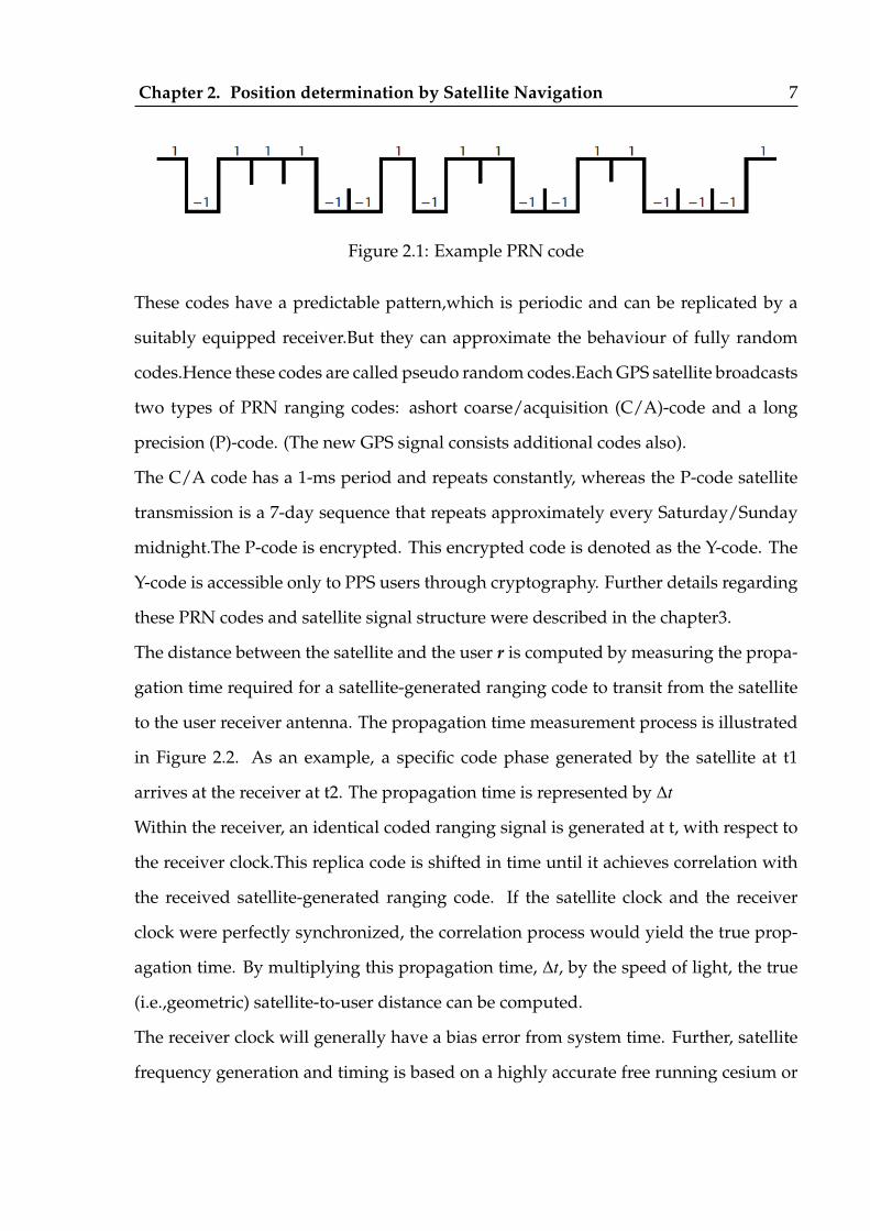
istic. A simple example of a short PRN code sequence is shown in Figure 2.1.
6
Chapter 2. Position determination by Satellite Navigation 7
Figure 2.1: Example PRN code
These codes have a predictable pattern,which is periodic and can be replicated by a
suitably equipped receiver.But they can approximate the behaviour of fully random
codes.Hence these codes are called pseudo random codes.Each GPS satellite broadcasts
two types of PRN ranging codes: ashort coarse/acquisition (C/A)-code and a long
precision (P)-code. (The new GPS signal consists additional codes also).
The C/A code has a 1-ms period and repeats constantly, whereas the P-code satellite
transmission is a 7-day sequence that repeats approximately every Saturday/Sunday
midnight.The P-code is encrypted. This encrypted code is denoted as the Y-code. The
Y-code is accessible only to PPS users through cryptography. Further details regarding
these PRN codes and satellite signal structure were described in the chapter3.
The distance between the satellite and the user r is computed by measuring the propa-
gation time required for a satellite-generated ranging code to transit from the satellite
to the user receiver antenna. The propagation time measurement process is illustrated
in Figure 2.2. As an example, a specific code phase generated by the satellite at t1
arrives at the receiver at t2. The propagation time is represented by ∆t
Within the receiver, an identical coded ranging signal is generated at t, with respect to
the receiver clock.This replica code is shifted in time until it achieves correlation with
the received satellite-generated ranging code. If the satellite clock and the receiver
clock were perfectly synchronized, the correlation process would yield the true prop-
agation time. By multiplying this propagation time, ∆t, by the speed of light, the true
(i.e.,geometric) satellite-to-user distance can be computed.
The receiver clock will generally have a bias error from system time. Further, satellite
frequency generation and timing is based on a highly accurate free running cesium or

Chapter 2. Position determination by Satellite Navigation 8
Figure 2.2: Use of replica code to determine satellite code transmission time.
rubidium atomic clock, which is typically offset from system time. Thus, the range de-
termined by the correlation process is denoted as the pseudorange ρ. The measurement
is called pseudorange because it is the range determined by multiplying the signal
propagation velocity, c, by the time difference between two nonsynchronized clocks
(the satellite clock and the receiver clock).The timing relationships are shown in Figure
2.3, where:
Ts = System time at which the signal left the satellite
Tu = System time at which the signal reached the user receiver

Chapter 2. Position determination by Satellite Navigation 9
δt = Offset of the satellite clock from system time [advance is positive; retardation (de-
lay) is negative]
tu = Offset of the receiver clock from system time
Ts + δt = Satellite clock reading at the time that the signal left the satellite
Tu + tu = User receiver clock reading at the time the signal reached the user receiver
c = speed of light
Figure 2.3: Range measurement timing relationships.
Geometric range, r = c(Tu - Ts) = c∆t
Pseudo range, ρ = c [(Tu + tu) − (Ts + δt)]
= c(Tu − Ts) + c(tu − δt)= r + c(Tu − δt)
The formulae for computing the geometric and pseudo ranges are shown above. Assum-
ing the satellite error was compensated,the pseudo range equation becomes

Chapter 2. Position determination by Satellite Navigation 10
ρ = ||s - u||+ ctu
where vector s represents the position of the satellite relative to the coordinate ori-
gin and it is located at coordinates xs,ys,zs within the ECEF(Earth-Centered Earth-
Fixed Coordinate System) Cartesian coordinate system.. Vector s is computed using
ephemeris data broadcast by the satellite.
And vector u,represents a user receivers position with respect to the ECEF coordinate
system origin. The users position coordinates xu, yu, zu are considered unknown.
2.2 Calculation of the User Position
In order to determine user position in three dimension(xu, yu, zu) and the offset tu.pseudorange
measurements are made to four satellites resulting in the system of equations.
ρ j = ||s - u||+ ctu
where j ranges from 1 to 4 and references the satellites. Above equation can be ex-
panded into the following set of equations in the unknowns xu, yu, zu and tu:
ρ1 =√
(x1 − xu)2 + (y1 − yu)2 + (z1 − zu)2
ρ2 =√
(x2 − xu)2 + (y2 − yu)2 + (z2 − zu)2
ρ3 =√
(x3 − xu)2 + (y3 − yu)2 + (z3 − zu)2
ρ4 =√
(x4 − xu)2 + (y4 − yu)2 + (z4 − zu)2
where x j, y j, andz j denote the jth satellites position in three dimensions.
These equations can be solved for user position u by linearisation of above equations
using taylor series expansion about an approximate user position.
After expanding the above equations about the approximate user position and consid-
ering the first order derivatives only the following matrix equation can be obtained.
∆ρ = H∆x

Chapter 2. Position determination by Satellite Navigation 11
where
∆ρ =
∆ρ1
∆ρ2
∆ρ3
∆ρ4
H =
ax1 ay1 az1 1
ax2 ay2 az2 1
ax3 ay3 az3 1
ax4 ay4 az4 1
∆x =
∆xu
∆yu
∆zu
−c∆tu
∆ρ and ∆x are the deviations of the actual user position from the approximate position
and (ax j, ay j, az j) are the direction cosines of the unit vector pointing from the approxi-
mate user position to the jth satellite.
So the user position can be found as follows.
∆x = H−1∆ρ
u = u + ∆x

Chapter 3
GPS signal structure and characteristics
The GPS signal format is known as direct sequence spread spectrum.The term direct se-
quence is used when the spreading of the spectrum is accomplished by phase modula-
tion of the carrier.This chapter will describe the modulations of GPS signal,Components
of GPS signal,and autocorrelation function of the Rectangular PRN codes and its ex-
ploitation for acquisition and tracking of GPS signal.
3.1 Modulations of GPS signal
BPSK
Binary phase shift keying (BPSK) is a simple digital signaling scheme in which an RF
carrier is either transmitted as it is or with a 180o phase shift over successive intervals
in time depending on whether a digital 0 or 1 is being conveyed an example is shown
in the figure 3.1.
BPSK signal, as illustrated in Figure 3.1, can be thought of as the product of two time
waveforms: the unmodulated RF carrier and a data waveform that takes on a value
of either +1 or -1 for each successive interval of Tb = 1/Rb seconds, where Rb is the
data rate in bits per second. The data waveform amplitude for the kth interval of
Tb seconds can be generated from the kth data bit to be transmitted using either the
12

Chapter 3. GPS signal structure and characteristics 13
Figure 3.1: BPSK modulation
mapping [0, 1]→ [−1,+1] or [0, 1]→ [+1,−1].
Direct Sequence Spread Spectrum
Direct sequence spread spectrum(DSSS) is an extension of BPSK or other phase shift keyed
modulation used by GPS and some other satellite navigation systems.The DSSS mod-
ulation waveforms are shown in the figure 3.2.
As shown in Figure 3.2, DSSS signaling adds a third component, referred to as a spread-
ing or PRN waveform, which is similar to the data waveform but at a much higher
symbol rate. This PRN waveform is completely known, at least to the intended re-
ceivers. The PRN waveform is often periodic, and the finite sequence of bits used to
generate the PRN waveform over one period is referred to as a PRN sequence or PRN
code. An overview of PRN codes, including their generation,characteristics, and code
families with good properties is provided in [1]. The minimum interval of time be-
tween transitions in the PRN waveform is commonly referred to as the chip period, Tc;
the portion of the PRN waveform over one chip period is known as a chip or spreading

Chapter 3. GPS signal structure and characteristics 14
Figure 3.2: DSSS modulation
symbol; and the reciprocal of the chip period is known as the chipping rate, Rc. The
independent time parameter for the PRN waveform is often expressed in units of chips
and referred to as codephase. The signal just described is called spread spectrum, be-
cause of the wider bandwidth occupied by the signal after modulation by the high-rate
PRN waveform. In general, the bandwidth is proportional to the chipping rate. There
are three primary reasons why DSSS waveforms are employed for satellite navigation.
First and most importantly, the frequent phase inversions in the signal introduced by
the PRN waveform enable precise ranging by the receiver.Second, the use of different
PRN sequences from a well-designed set enables multiple satellites to transmit signals
simultaneously and at the same frequency. A receiver can distinguish among these
signals, based on their different codes. For this reason, the transmission of multiple
DSSS signals having different spreading sequences on a common carrier frequency is
referred to as code division multiple access (CDMA). Finally DSSS provides signifi-
cant rejection of narrowband interference. The chip waveform in a DSSS signal does

Chapter 3. GPS signal structure and characteristics 15
not need to be rectangular (i.e., a constant amplitude over the chip period).In princi-
ple, any shape could be used and different shapes can be used for different chips.DSSS
signals generated using BPSK signaling with rectangular chips as BPSK-R signals. Sev-
eral variations of the basic DSSS signal that employ nonrectangular symbols have been
investigated for satellite navigation applications in recent years. Binary offset carrier
(BOC) signals are generated using DSSS techniques but employ portions of a square
wave for the spreading symbols [2].
3.2 GPS Signal Structure
The GPS Satellites(refer to as SV’s) transmit navigation signals on two carrier frequen-
cies called L1, the primary frequency, and L2, the seconda ry frequency. The carrier
frequencies are DSSS modulated by spread spectrum codes with unique PRN(Pseudo
Random Noise) sequences associated with each SV and by a common navigation data
message. All SVs transmit at the same carrier frequencies in a CDMA fashion. In or-
der to track one SV in common view with several other SVs by the CDMA technique, a
GPS receiver must replicate the PRN sequence for the desired SV along with the replica
carrier signal,including Doppler effects. Two carrier frequencies are required to mea-
sure the ionospheric delay, since this delay is related by a scale factor to the difference
in signal TOA(time of arrival) for the two carrier frequencies. Single frequency users
must estimate the ionospheric delay using modeling parameters that are broadcast to
the user in the navigation message.
3.2.1 Frequencies,Modulation Format and PRN codes
A block diagram that is representative of the SV signal structure for L1 (154 f0) and L2
(120 f0) is shown in Figure 3.3 (where f0 is the fundamental frequency: 10.23MHz).
As shown in Figure 3.3, the L1 frequency (154 f0) is modulated by two PRN codes
(plus the navigation message data), the C/A code, and the P code. The L2 frequency

Chapter 3. GPS signal structure and characteristics 16
(120 f0) is modulated by only one PRN code at a time. One of the P code modes has
no data modulation. The nominal reference frequency, f0, as it appears to an observer
on the ground, is 10.23 MHz. To compensate for relativistic effects, the output of the
SV’s frequency standard (as it appears from the SV) is 10.23 MHz offset by a ∆ f /f of
4.467×10⁻¹⁰. This results in a ∆ f of 4.57 ×10⁻³Hz and f0 = 10.22999999543 MHz. To the
GPS receiver on the ground, the C/A code has a chipping rate of 1.023 ×10⁶ chips/s
( f0/10 = 1.023 MHz) and the P code has a chipping rate of 10.23 ×10⁶ chips/s ( f0 = 10.23
MHz).The C/A code signal uses a BPSK-R(1) (means BPSK modulation using 1MHz
chipping rate) modulation and the P code uses a BPSK-R(10) modulation.Where The P
code is available only to specific users such as military.
Figure 3.3: GPS signal structure
As figure 3.3 shows the same 50-bps navigation message data is combined with both

Chapter 3. GPS signal structure and characteristics 17
the C/A code and the P(Y) code prior to modulation with the L1 carrier. An exclusive-
or logic gate is used for this modulation process, denoted by �. Since the C/A code
� data and P(Y) code � data are both synchronous operations, the bit transition rate
cannot exceed the chipping rate of the PRN codes. Also note that BPSK modulation is
used with the carrier signals. The P(Y) code � data is modulated in phase quadrature
with the C/A code � data on L1. As shown in Figure 3.3, the L1 carrier is phase shifted
90o before being BPSK modulated by the C/A code� data.Then this result is combined
with the attenuated output of the BPSK modulation of L1 by the P(Y) code � data. The
3-dB amplitude difference and phase relationship between P code and C/A code on L1
are illustrated by the vector phase diagram in Figure 3.4. Figure 3.5 illustrates the result
of P code � data and C/A � data. As observed in Figure 3.4, the exclusive-or process
is equivalent to binary multiplication of two 1-bit values yielding a 1-bit product using
the convention that logical 0 is plus and logical 1 is minus.
There are 204,600 P(Y) code epochs between data epochs and 20,460 C/A code epochs
between data epochs, so the number of times that the phase could change in the PRN
code sequences due to data modulation is relatively infrequent, but the spectrum changes
due to this modulation are very significant.
There are 154 carrier cycles per P(Y) code chip and 1,540 carrier cycles per C/A code
chip on L1, so the phase shifts on the L1 carrier are relatively infrequent.The L2 fre-
quency (1,227.60 MHz) can be modulated by either the P(Y) code � data or the C/A
code � data or by the P(Y) code alone as selected by the CS(Ground based Control
sigment which monitors and controls the satellite navigation). The P(Y) code and C/A
codes are never present simultaneously on L2 prior to GPS modernization unlike the
case with L1. In general, the P(Y) code � data is the one selected by the CS. There are
120 carrier cycles per P(Y) code chip on L2, so the phase transitions on the L2 carrier
are relatively infrequent. Table 3.1 summarizes the GPS signal structure on L1 and L2.

Chapter 3. GPS signal structure and characteristics 18
Figure 3.4: Vector diagram of L1 GPS signal
Figure 3.5: GPS code mixing with data

Chapter 3. GPS signal structure and characteristics 19
Parameter C/A-code P-codeChipping rate 1.023×106 bits per sec-
ond10.23 ×106 bits persecond
Chip length ≈ 300m ≈ 30mRepetition rate 1 Millisecond one weekCode type 37 unique codes 37 one-week seg-
mentsProperties Easy to acquire More accurate
Table 3.1: PRN codes characteristics
3.3 Autocorrelation and PSD functions of random sequence
of pulses
The autocorrelation function of a signal is defined as
R(τ) = limT→∞
12T
∫ T
−Ts(t)s(t − τ) dt (3.1)
From the above definition the autocorrelation function of a random sequence of rect-
angular chips(pulses), each of amplitude A and width Tc is given by the following
formula.
R(τ) =
A2(1 − |τ|Tc
)for|τ| ≤ Tc
0 elsewhere(3.2)
The power spectral density is defined to be the Fourier transform of the autocorrelation
function:
S ( f ) =
∫ ∞
−∞R(τ)e− j2π f τ dτ (3.3)
Hence the power spectral density(PSD) of a random sequence of pulses is given by
S ( f ) = A2Tcsinc2(π f Tc) (3.4)
where sinc(x) =sin(x)
x .
An example of a random sequence of rectangular pulses,its autocorrelation function,
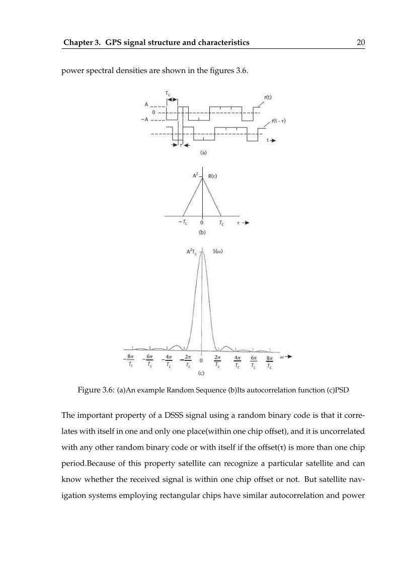
Chapter 3. GPS signal structure and characteristics 20
power spectral densities are shown in the figures 3.6.
Figure 3.6: (a)An example Random Sequence (b)Its autocorrelation function (c)PSD
The important property of a DSSS signal using a random binary code is that it corre-
lates with itself in one and only one place(within one chip offset), and it is uncorrelated
with any other random binary code or with itself if the offset(τ) is more than one chip
period.Because of this property satellite can recognize a particular satellite and can
know whether the received signal is within one chip offset or not. But satellite nav-
igation systems employing rectangular chips have similar autocorrelation and power

Chapter 3. GPS signal structure and characteristics 21
spectrum properties to those described for the random binary code case, but they em-
ploy PRN codes that are perfectly predictable and reproducible. This is why they are
called pseudo random codes.
3.3.1 Effect of finite length PRN code on the autocorrelation function
and PSD
Because of the finite length of the PRN codes used by satellites the code repeats after
every finite interval N (but approximate random nature within this interval).Hence the
the autocorrelation function described above will become periodic with period N and
function out side the chip period won’t completely vanish.
So the actual autocorrelation function for PRN sequence is given by
RPN(τ) =
A2(1 − |τ|Tc
(1 + 1
N
))for|τ − nTc| ≤ Tc
− 1N elsewhere
(3.5)
where n = 0,±1,±2,±3,.......
This function and its PSD are shown in the figure 3.7.
Figure 3.7: (a)Autocorrelation function of a PRN sequence (b)Its PSD

Chapter 4
GPS Receiver Channel
The ultimate goal of GPS is to provide position,velocity,and time.To achieve these the
primary tasks it has to perform are measurement of range and range-rate and demod-
ulation of the navigation data. The navigation data are the 50-bits/s data stream mod-
ulated onto the GPS signal. The navigation data contain the satellite clock and orbital
parameters which are used in the computation of user position.
4.1 Analog front end of GPS receiver
Most modern GPS receiver designs are digital receivers. Block diagram of a digital
GPS receiver is shown in figure 4.1. The GPS RF signals of all SVs in view are received
by a RHCP(right hand circularly polarized) antenna with nearly hemispherical (i.e.,
above the local horizon) gain coverage. These RF signals are amplified by a low noise
preamplifier (preamp), which effectively sets the noise figure of the receiver. There
may be a passive bandpass prefilter between the antenna and preamp to minimize
out-of-band RF interference. These amplified and signal conditioned RF signals are
then down-converted to an IF using signal mixing frequencies from local oscillators
(LOs).
The LOs are derived from the reference oscillator by the frequency synthesizer, based
22

Chapter 4. GPS Receiver Channel 23
Figure 4.1: Generic digital GPS receiver block diagram.
on the frequency plan of the receiver design. One LO per downconverter stage is re-
quired. The LO signal mixing process generates both upper and lower sidebands of
the SV signals, so the lower sidebands are selected and the upper sidebands and leak-
through signals are rejected by a postmixer bandpass filter. The signal Dopplers and
the PRN codes are preserved after the mixing process. Only the carrier frequency is
lowered, but the Doppler remains referenced to the original L-band signal. The A/D
conversion process and automatic gain control (AGC) functions take place at IF. Not
shown in the block diagram are the baseband timing signals that are provided to the
digital receiver channels by the frequency synthesizer phase locked to the reference
oscillators stable frequency. The IF must be high enough to provide a single-sided
bandwidth that will support the PRN code chipping frequency. An antialiasing IF fil-
ter must suppress the stopband noise (unwanted out-of-band signals) to levels that are
acceptably low when this noise is aliased into the GPS signal passband by the A/D
conversion process. The signals from all GPS satellites in view are buried in thermal

Chapter 4. GPS Receiver Channel 24
noise at IF. At this point the digitized IF signals are ready to be processed by each of
the N digital receiver channels. No demodulation has taken place, only signal gain and
conditioning plus A/D conversion into the digital IF.
This digitized IF signal will be processed by a set of channels which will normally
implemented on ASIC or FPGA.A channel may be assigned to a single satellite or
multiple channels using multiplexing depending upon the availability of hardware
resources.The next section describes the detailed GPS receiver channel architecture.
4.2 Digital receiver channel
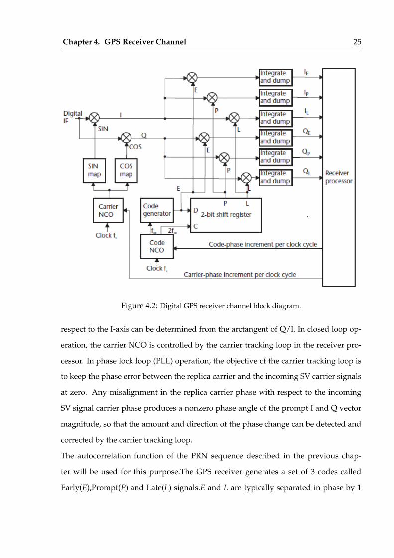
Figure 4.2 illustrates a high-level block diagram typical of one of the digital receiver
channels where the digitized received IF signal is applied to the input. For simplifi-
cation, only the functions associated with the code and carrier tracking loops are il-
lustrated, and the receiver channel is assumed to be tracking the SV signal in steady
state. Referring to Figure 4.2, first the digital IF is stripped of the carrier (plus carrier
Doppler) by the replica carrier (plus carrier Doppler) signals to produce in-phase (I)
and quadraphase (Q) sampled data. Note that the replica carrier signal is being mixed
with all of the in-view GPS SV signals (plus noise) at the digital IF.The I and Q signals
at the outputs of the mixers have the desired phase relationships with respect to the
detected carrier of the desired SV.
The NCO shown in the figure is described in the next section.This produces a stair-
case function whose period is the desired replica carrier plus Doppler period. The sine
and cosine map functions convert each discrete amplitude of the staircase function to
the corresponding discrete amplitude of the respective sine and cosine functions. By
producing I and Q component phases 90 apart, the resultant signal amplitude can be
computed from the vector sum of the I and Q components, and the phase angle with
Chapter 4. GPS Receiver Channel 25
Figure 4.2: Digital GPS receiver channel block diagram.
respect to the I-axis can be determined from the arctangent of Q/I. In closed loop op-
eration, the carrier NCO is controlled by the carrier tracking loop in the receiver pro-
cessor. In phase lock loop (PLL) operation, the objective of the carrier tracking loop is
to keep the phase error between the replica carrier and the incoming SV carrier signals
at zero. Any misalignment in the replica carrier phase with respect to the incoming
SV signal carrier phase produces a nonzero phase angle of the prompt I and Q vector
magnitude, so that the amount and direction of the phase change can be detected and
corrected by the carrier tracking loop.
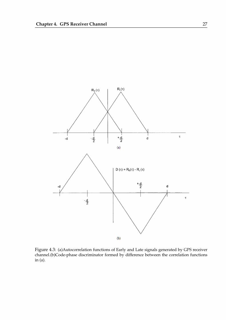
The autocorrelation function of the PRN sequence described in the previous chap-
ter will be used for this purpose.The GPS receiver generates a set of 3 codes called
Early(E),Prompt(P) and Late(L) signals.E and L are typically separated in phase by 1

Chapter 4. GPS Receiver Channel 26
chip and P is in the middle. Correspondingly the autocorrelation functions for the E
and L signals will be shifted left and right respectively by half chip period as shown
the figure 4.3.
In Figure 4.2, the I and Q signals are correlated with early, prompt, and late replica
codes (plus code Doppler) synthesized by the code generator, a 2-bit shift register, and
the code NCO. In closed loop operation, the code NCO is controlled by the code track-
ing loop in the receiver processor.The code NCO produces twice the code generator
clocking rate, 2 fco, and this is fed to the clock input of the 2-bit shift register. The
code generator clocking rate, fco, that contains the nominal spreading code chip rate
(plus code Doppler) is fed to the code generator. The NCO clock, fc, should be a much
higher frequency than the shift register clock, 2 fco.With this combination, the shift reg-
ister produces two phase-delayed versions of the code generator output. As a result,
there are three replica code phases designated as early (E), prompt (P), and late (L).
Not shown are the controls to the code generator that permit the receiver processor to
preset the initial code tracking phase states that are required during the code search
and acquisition (or reacquisition) process.The prompt replica code phase is aligned
with the incoming SV code phase producing maximum correlation if it is tracking the
incoming SV code phase. Under this circumstance, the early phase is aligned a frac-
tion of a chip period early, and the late phase is aligned the same fraction of the chip
period late with respect to the incoming SV code phase, and these correlators produce
about half the maximum correlation. Any misalignment in the replica code phase with
respect to the incoming SV code phase produces a difference in the vector magnitudes
of the early and late correlated outputs so that the amount and direction of the phase
change can be detected and corrected by the code tracking loop as shown figure 4.3.
When the PLL is phase locked, the I signals are maximum (signal plus noise) and the
Q signals are minimum (containing only noise).
Chapter 4. GPS Receiver Channel 27
Figure 4.3: (a)Autocorrelation functions of Early and Late signals generated by GPS receiverchannel.(b)Code-phase discriminator formed by difference between the correlation functionsin (a).

Chapter 4. GPS Receiver Channel 28
Predetection Integration
Predetection is the signal processing after the IF signal has been converted to base-
band by the carrier and code stripping processes, but prior to being passed through
a signal discriminator. Extensive digital predetection integration and dump processes
occur after the carrier and code stripping processes. This causes very large numbers
to accumulate, even when 1 to 3 bits of quantization resolutions are used for IF A/D
conversion.The code wipeoff process that follows usually involving only 1-bit mul-
tiplication.Figure 4.2 shows three complex correlators required to produce three in-
phase components, which are integrated and dumped to produce IE, IP, IL and three
quadraphase components integrated and dumped to produce QE,QP,QL. The carrier
wipeoff and code wipeoff processes must be performed at the digital IF sample rate,
which is of the order of 50 MHz for a military P(Y) code receiver (that also operates
with C/A code), 5 MHz for civil C/A code receivers that use 1-chip E-L correlator
spacing, and up to 50 MHz for civil C/A code receivers that use narrow correlator
spacing for improved multipath error performance. The integrate and dump accumu-
lators provide filtering and resampling at the processor baseband input rate, which can
be at 1,000 Hz during search modes or as low as 50 Hz during track modes, depend-
ing on the desired dwell time during search or the desired predetection integration
time during track.The hardware integrate and dump process in combination with the
baseband signal processing integrate and dump process defines the predetection inte-
gration time.Predetection integration time is a compromise design. It must be as long
as possible to operate under weak or RF interference signal conditions, and it must be
as short as possible to operate under high dynamic stress signal conditions.

Chapter 4. GPS Receiver Channel 29
4.3 Frequency Synthesizer
The local carrier and code frequencies are synthesized from a high frequency source
in the receiver using a numerically controlled oscillator(NCO).Figure 4.4. shows the
block diagram of a frequency synthesizer.
Figure 4.4: frequency synthesizer block diagram.
The NCO consists a hold register of fixed number of bits.In each clock cycle the value
hold by this register will be incremented by fixed value M which will be determined
by the frequency selection as follows.If the desired output frequency is fop and hold
register is of size N bits.After every 2N/M clock cycles the hold register overflows and
reset to 0.Hence the frequency will be divided by 2N/M.Hence M value can be obtained
using the following formula M = fop2N
fs.Where fs is the receivers clock frequency.One
replica carrier cycle and one replica code cycle are completed each time the NCO over-
flows.The NCO phase diagram,cos and sin map diagrams are shown in figure 4.5.
The number of bits, j, is determined for the sin and cos outputs. The phase plane of
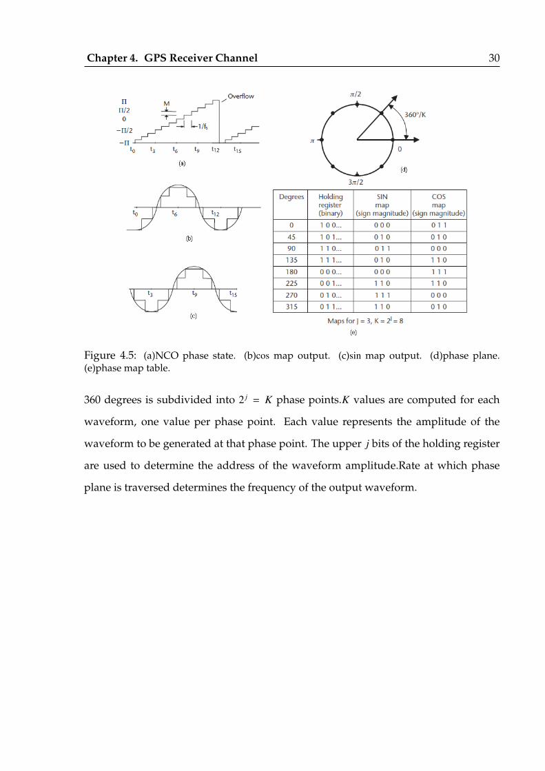
Chapter 4. GPS Receiver Channel 30
Figure 4.5: (a)NCO phase state. (b)cos map output. (c)sin map output. (d)phase plane.(e)phase map table.
360 degrees is subdivided into 2 j = K phase points.K values are computed for each
waveform, one value per phase point. Each value represents the amplitude of the
waveform to be generated at that phase point. The upper j bits of the holding register
are used to determine the address of the waveform amplitude.Rate at which phase
plane is traversed determines the frequency of the output waveform.

Chapter 5
Design of PRN code generators
Figure 5.1 depicts a high-level block diagram of the direct sequence PRN code genera-
tion used for GPS C/A code and P code generation to implement the CDMA technique.
Each synthesized PRN code is derived from two other code generators. In each case,
Figure 5.1: General PRN code generator block diagram.
31
Chapter 5. Design of PRN code generators 32
the second code generator output is delayed with respect to the first before their out-
puts are combined by an exclusive-or circuit. The amount of delay is different for each
SV. In the case of P code, the integer delay in P-chips is identical to the PRN number.
For C/A code, the delay is unique to each SV, so there is only a table lookup relation-
ship to the PRN number. These delays are summarized in Table 5.1. The C/A code
delay can be implemented by a simple but equivalent technique that eliminates the
need for a delay register. This technique is explained in the following paragraphs.
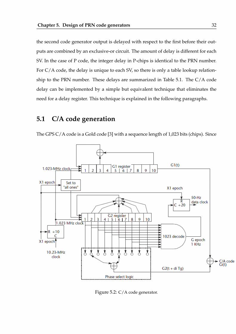
5.1 C/A code generation
The GPS C/A code is a Gold code [3] with a sequence length of 1,023 bits (chips). Since
Figure 5.2: C/A code generator.
Chapter 5. Design of PRN code generators 33
the chipping rate of the C/A code is 1.023 MHz, the repetition period of the pseu-
dorandom sequence is 1,023/(1.023×106Hz) or 1 ms. Figure 5.2 illustrates the design
architecture of the GPS C/A code generator.
Not included in this diagram are the controls necessary to set or read the phase states
of the registers or the counters. There are two 10-bit shift registers, G1 and G2, which
generate maximum length PRN codes with a length of 210 − 1 = 1,023 bits. (The only
state not used is the all-zero state). It is common to describe the design of linear code
generators by means of polynomials of the form 1 +∑
Xi, where Xi means that the
output of the ith cell of the shift register is used as the input to the modulo-2 adder
(exclusive-or), and the 1 means that the output of the adder is fed to the first cell. The
design specification for C/A code calls for the feedback taps of the G1 shift register to
be connected to stages 3 and 10. These register states are combined with each other by
an exclusive-or circuit and fed back to stage 1. The polynomial that describes this shift
register architecture is: G1 = 1 + X3 + X10. The polynomials and initial states for both
the C/A-code and P-code generator shift registers are summarized in Table 5.2.
The unique C/A code for each SV is the result of the exclusive-or of the G1 direct out-
put sequence and a delayed version of the G2 direct output sequence. The equivalent
delay effect in the G2 PRN code is obtained by the exclusive-or of the selected positions
of the two taps whose output is called G21. This is because a maximum-length PRN
code sequence has the property that adding a phase-shifted version of itself produces
the same sequence but at a different phase. The function of the two taps on the G2 shift
register in Figure 5.2 is to shift the code phase in G2 with respect to the code phase in
G1 without the need for an additional shift register to perform this delay. Each C/A
code PRN number is associated with the two tap positions on G2. Table 5.1 describes
these tap combinations for all defined GPS PRN numbers and specifies the equivalent
direct sequence delay in C/A code chips. The first 32 of these PRN numbers are re-
served for the space segment. Five additional PRN numbers, PRN 33 to PRN 37, are

Chapter 5. Design of PRN code generators 34
reserved for other uses, such as ground transmitters (also referred to as pseudosatel-
lites or pseudolites). C/A codes 34 and 37 are identical.
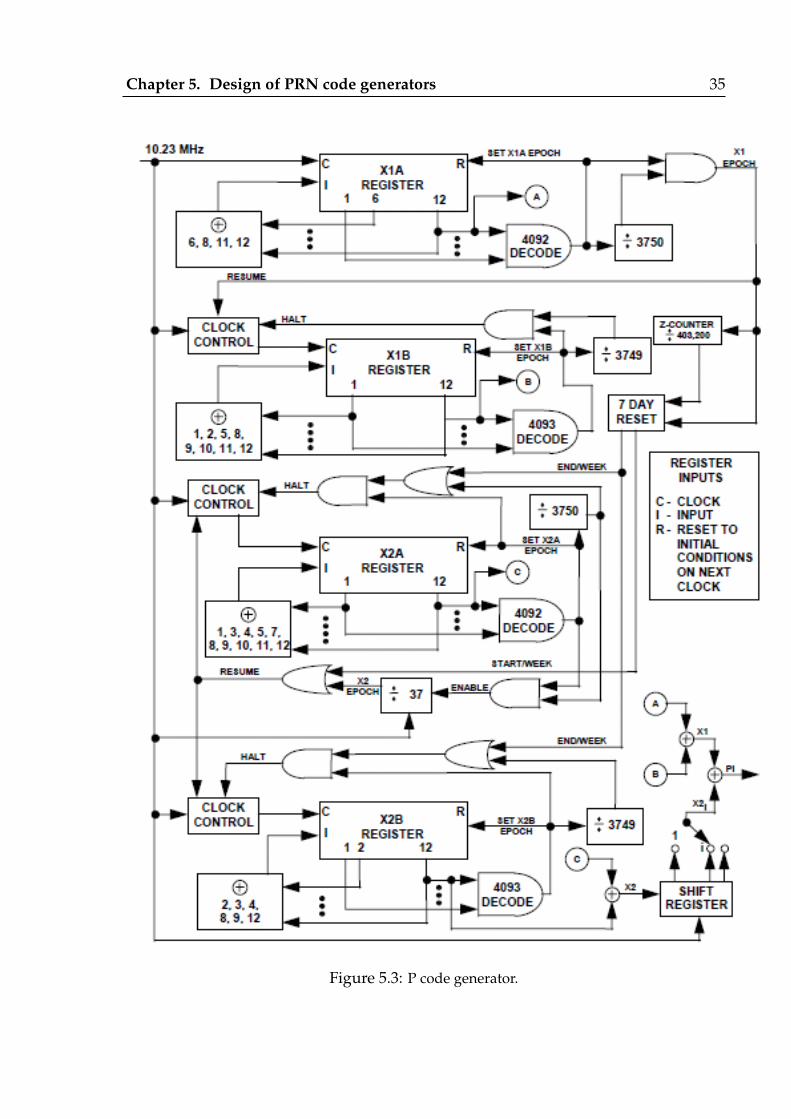
5.2 P code generation
The GPS P code is a PRN sequence generated using four 12-bit shift registers desig-
nated X1A, X1B, X2A, and X2B. A detailed block diagram of this shift register architec-
ture is shown in figure 5.3 [4]. Not included in this diagram are the controls necessary
to set or read the phase states of the registers and counters. This reset and clock control
logic were shown in figure 5.4. The X1A register output is combined by an exclusive-
or circuit with the X1B register output to form the X1 code generator and that the X2A
register output is combined by an exclusive-or circuit with the X2B register output to
form the X2 code generator.The composite X2 result is fed to a shift register delay of
the SV PRN number in chips and then combined by an exclusive-or circuit with the X1
composite result to generate the P code. The design specification for the P code calls for
each of the four shift registers to have a set of feedback taps that are combined by an
exclusive-or circuit with each other and fed back to their respective input stages. The
polynomials that describe the architecture of these feedback shift registers are shown
in Table 5.2, and the logic diagram is shown in detail in Figure 5.3. As shown in Figure
5.3,the natural cycles of all four feedback shift registers are truncated. For example,
X1A and X2A are both reset after 4,092 chips,eliminating the last three chips of their
natural 4,095 chip sequences. The registers X1B and X2B are both reset after 4,093 chips,
eliminating the last two chips of their natural 4,095 chip sequences. This results in the
phase of the X1B sequence lagging by one chip with respect to the X1A sequence for
each X1A register cycle. As a result, there is a relative phase precession between the
X1A and X1B registers. A similar phase precession takes place between X2A and X2B.
At the beginning of the GPS week, all of the shift registers are set to their initial states
simultaneously, as shown in Table 5.2.
Chapter 5. Design of PRN code generators 35
Figure 5.3: P code generator.

Chapter 5. Design of PRN code generators 36
Halt
Resume
Q
Clk_cntrl
Reset
Clk
D
Rst
En
Figure 5.4: clock control circut shown in figure 5.3.
Also, at the end of each X1A epoch, the X1A shift register is reset to its initial state. At
the end of each X1B epoch, the X1B shift register is reset to its initial state. At the end of
each X2A epoch, the X2A shift register is reset to its initial state. At the end of each X2B
epoch, the X2B shift register is reset to its initial state. The outputs (stage 12) of the A
and B registers are combined by an exclusive-or circuit to form an X1 sequence derived
from X1A � X1B, and an X2 sequence derived from X2A � X2B. The X2 sequence is
delayed by i chips (corresponding to SVi) to form X2i. The P code for SVi is Pi = X1 �X2i.
There is also a phase precession between the X2A/X2B shift registers with respect to
the X1A/X1B shift registers. This is manifested as a phase precession of 37 chips per
X1 period between the X2 epochs (shown in Figure 5.3 as the output of the divide by
37 counter) and the X1 epochs. This is caused by adjusting the X2 period to be 37
chips longer than the X1 period. The details of this phase precession are as follows.
The X1 epoch is defined as 3,750 X1A cycles. When X1A has cycled through 3,750 of
these cycles, or 3,750×4,092 = 15,345,000 chips, a 1.5-second X1 epoch occurs. When
X1B has cycled through 3,749 cycles of 4,093 chips per cycle, or 15,344,657 chips, it is
kept stationary for an additional 343 chips to align it to X1A by halting its clock control
until the 1.5-second X1 epoch resumes it. Therefore, the X1 registers have a combined
period of 15,345,000 chips. X2A and X2B are controlled in the same way as X1A and

Chapter 5. Design of PRN code generators 37
Table 5.1: Code Phase AssignmentsSV PRN C/A-code Tap C/A-code P codeNumber Selection delay(chips) delay(chips)1 2�6 5 12 3�7 6 23 4�8 7 34 5�9 8 45 1�9 17 56 2�6 18 67 1�8 139 78 2�9 140 89 3�10 141 910 2�3 251 1011 3�4 252 1112 5�6 254 1213 6�7 255 1314 7�8 256 14. . . .. . . .. . . .. . . .33 5�10 863 3334 4�10 9503 3435 1�7 947 3536 2�8 948 3637 4�10 9503 37
X1B, respectively, but with one difference: when 15,345,000 chips have completed in
exactly 1.5 seconds, bothX2A andX2B are kept stationary for an additional 37 chips
by halting their clock controls until the X2 epoch or the start of the week resumes
it. Therefore, theX2 registers have a combined period of 15,345,037 chips, which is 37
chips longer than the X1 registers.Note that if the P code were generated by X1 .X2, and
if it were not reset at the end of the week, it would have the potential sequence length
of 15,345,000× 15,345,037 = 2.3547×10¹⁴ chips. With a chipping rate of 10.23×10⁶, this
sequence has a period of 266.41 days or 38.058 weeks. However, since the sequence is
truncated at the end of the week, each SV uses only one week of the sequence, and 38
unique one-week PRN sequences are available. The sequence length of each P code,

Chapter 5. Design of PRN code generators 38
Table 5.2: GPS Code Generator Polynomials and Initial StatesRegister Polynomial Initial StateC/A code G1 1 + X3 + X10 1111111111C/A code G2 1 + X2 + X3 + X6 + X8 + X9 + X10 1111111111P code X1A 1 + X6 + X8 + X11 + X12 001001001000P code X1B 1 + X1 + X2 + X5 + X8 + X9 + X10 + X11 + X12 010101010100P code X2A 1 + X1 + X3 + X4 + X5 + X7 + X8 + X9 + X10 + X11 + X12 100100100101P code X2B 1 + X2 + X3 + X4 + X8 + X9 + X12 010101010100
with the truncation to a 7-day period, is 6.1871×10¹² chips. As in the case of C/A code,
the first 32 PRN sequences are reserved for the space segment and PRN 33 through 37
are reserved for other uses (e.g., pseudolites). The PRN 38 P code is sometimes used
as a test code in P(Y) code GPS receivers, as well as to generate a reference noise level
(since, by definition, it cannot correlate with any used SV PRN signals). The unique P
code for each SV is the result of the different delay in the X2 output sequence. Table
5.1 shows this delay in P code chips for each SV PRN number.The P code delays (in
P code chips) are identical to their respective PRN numbers for the SVs, but the C/A
code delays (in C/A code chips) are different from their PRN numbers. The C/A code
delays are typically much longer than their PRN numbers. The replica C/A codes for
a conventional GPS receiver can be synthesized by programming the tap selections on
the G2 shift register.
5.3 Correlation results of the implemented GPS receiver
channel
According to the specifications of PRN code generation described in this chapter and
receiver channel architecture described in chapter 4 a receiver channel is implemented
using xilinx system generator.Using this channel the correlation values of incoming
signal for various phase delays are obtained.The incoming signal is modeled by giving
variable delay before being fed to the receiver channel input.The results are shown in

Chapter 5. Design of PRN code generators 39
the figure 5.5.
0 10 20 30 40 50 60 70−2.5
−2
−1.5
−1
−0.5
0
0.5x 10
4
Code phase offset
Correlation of the received signal with Early,Prompt,and Late C/A code Vs Code phase offset
IeIpIlQeQpQl
Figure 5.5: Correlation results with Early,Prompt,and Late signals
Chapter 6
Subchip Multipath Delay Estimation
using TeagerKaiser Operator
Traditional approaches used for channel estimation generally fail in estimating closely-
spaced multipath components in code-division multiple access (CDMA) systems. Ap-
plication of Teager-Kaiser operator[8] for downlink WCDMA multipath delay estima-
tion is a highly efficient technique with subchip resolution capability.[5].This technique
has the advantage of simplicity and efficiency compared to the other available tech-
niques.But the performance of this technique is influenced by the shape of the pulse
waveform used.It performs well for rectangular pulse than other pulse shapes.This
will be described in the following sections.
6.1 Signal and Channel Model
In a downlink DS-CDMA scenario with K users in the system, the received signal can
be written as [9].
r(t) =
K∑
k=1
√Pk
∞∑
n=−∞bn,k
L∑
l=1
αn,lsnk(t − τn,l) + η(t) (6.1)
where
40

Chapter 6. Subchip Multipath Delay Estimation using TeagerKaiser Operator 41
Pk is the power of user k.bn,k is the transmitted data symbol n of user k. αn,l and τn,l are
the complex attenuation coefficient and delay,repectively, of the l th path during the
symbol n. L is the number of channel paths.snk(.) is the signature of user k during the
symbol n. η(.) is the complex additive white Gaussian noise.
The user signatures are expressed as follows.
snk(t) =
S Fk−1∑
m=0
cnm,k p(t − mTc − nS FkTc) (6.2)
where cnm,k is the code value of m th chip of user k during the symbol n, Tc is the chip
interval, p(.) is the chip pulse shape, S Fk is the spreading factor of user k.
Delay estimation is based on the cross-correlation between the received signal r(t) and
the replica of the desired user signature. The output of the correlator is given by [11].
yn(τ) =√
Pkbn,k
L∑
l=1
αn,lR(τ − τn,l) + η(τ) (6.3)
where η(.) is an additive Gaussian noise process incorporating the effects of noise, mul-
tiuser interference, interpath and intersymbol interference, and R(τ) is the pulse shape
autocorrelation function, which is given for a rectangular pulse shape by equation 3.2.
Equation 6.3 implies that for rectangular pulse shape, the output of the correlator is
a superposition of shifted triangular pulses weighted by the complex channel tap co-
efficients and the data modulation within some additive noise. To avoid the effect of
multipaths the contribution of interfering paths must be subtracted from the output
of the finger tracking the path of interest.For that we need to know these multipath
delays.

Chapter 6. Subchip Multipath Delay Estimation using TeagerKaiser Operator 42
There are several delay estimation algorithms available for estimating these delays[5].
The performance of the delay estimators is defined by the error statistics such as the
acquisition probability(probability of estimating all multipath delays within a certain
fixed error limit), the mean or the variance of the error,root mean square error (RMSE)
of the multipath delays etc.
TK based algorithm is one of the highly efficient techniques[6] with additional advan-
tage of lowest complexity.It will give best performance for rectangular pulse shape.The
description of this Operator and the results obtained using this operator are shown in
the following section.
6.2 Teager-Kaiser Operator and its application for the De-
lay Estimation
The nonlinear quadratic TK operator was first introduced for measuring the real phys-
ical energy of a system[7].Since its introduction, several other applications have been
found for TK operator.
The Structure of the correlation function 6.3 can be exploited with the aid of the non-
linear TK operator[8] ψ[.] defined below for continuous time function.
ψC[x(t)] = x(t)x∗(t) − 12
[x(t)x∗(t) + x(t)x∗(t)]. (6.4)
Similarly, the discrete-time Teager operator of a complex valued signal is given by[10]
ψD[x(n)] = x(n − 1)x∗(n − 1) − 12
[x(n − 2)x∗(n) + x(n)x∗(n − 2)]. (6.5)
For a real signal equation 6.5 comes into very simple form as
ψD[x(n)] = x2(n − 1) − x(n)x(n − 2). (6.6)

Chapter 6. Subchip Multipath Delay Estimation using TeagerKaiser Operator 43
By applying the continuous TK operator to 6.3, the following equation can be obtained.
ψC[yn(τ)] =1Tc
L∑
l=1
L∑
j=1
Re[αn,lα∗n, j]R(τ − τn,l) × δ(τ − τn,l)
+1
T 2C
L∑
l=1
L∑
j=1
αn,lα∗n, j × sign((τ − τn,l)(τ − τn,j)) × Π(τ − τn,l,Tc) × Π(τ − τn,j,Tc)
+ ηT K(τ).
Π(t,Tc) =
1 |t| ≤ Tc
0 otherwise(6.7)
where Π(t,Tc) stands for a rectangular function with unit amplitude and duration 2Tc
centered at τ = 0. δ(τ) stands for the Dirac function,and ηT K(τ)is the additive white
Gaussian noise at the output of the TK operator.
This δ(.) function is the result of the sharp edges of the rectangular pulse shape. i.e The
performance of this tecqnique is influenced by the pulse shape.
From equation 6.7 it is very clear that the TK operator applied to the output of the
correlator provides clear time-aligned peak locations of the closely spaced paths in the
presence of a certain ”noise” floor [second and third terms of 6.7].
Chapter 6. Subchip Multipath Delay Estimation using TeagerKaiser Operator 44
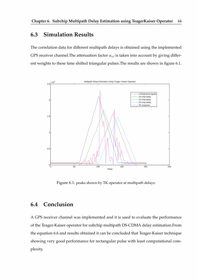
6.3 Simulation Results
The correlation data for different multipath delays is obtained using the implemented
GPS receiver channel.The attenuation factor αn,l is taken into account by giving differ-
ent weights to these time shifted triangular pulses.The results are shown in figure 6.1.
0 50 100 150 200 2500
0.5
1
1.5
2
2.5x 10
4
Delay
Multipath Delay Estimation Using Teager−Kaiser Operator.
LOS(desired signal)1/4 chip delay1/2 chip delay0.9 chip delayTK response
Figure 6.1: peaks shown by TK operator at multipath delays.
6.4 Conclusion
A GPS receiver channel was implemented and it is used to evaluate the performance
of the Teager-Kaiser operator for subchip multipath DS-CDMA delay estimation.From
the equation 6.6 and results obtained it can be concluded that Teager-Kaiser technique
showing very good performance for rectangular pulse with least computational com-
plexity.

Chapter 6. Subchip Multipath Delay Estimation using TeagerKaiser Operator 45
6.5 Future Work
Teager-Kaiser method is showing excellent performance for rectangular pulse with
least computational complexity.Efficient algorithms must be designed to make it in-
dependent of the pulse shape for showing high performance.This can be done by com-
bining this technique with other efficient but complex techniques and optimizing the
performance.
Bibliography
[1] Simon, M., et al., Spread Spectrum Communications Handbook, New York:
McGraw-Hill,1994.
[2] Betz, J., ”Binary Offset Carrier Modulations for Radionavigation,” NAVIGATION:
Journal of The Institute of Navigation, Vol. 48, No. 4, Winter 20012002.
[3] Gold, R., ”Optimal Binary Sequences for Spread Spectrum Multiplexing,” IEEE
Trans. on Information Theory, Vol. 33, No. 3, 1967.
[4] ARINC, NAVSTAR GPS Space Segment/Navigation User Interfaces, IS-GPS-
200D, ARINC Research Corporation, Fountain Valley, CA, December 7, 2004.
[5] E. S. Lohan, R.Hamila, A. Lakhzouri, and M. Renfors, ”Highly efficient techniques
for mitigating the effects of multipath propagation in DS-CDMA delay estima-
tion,” IEEE Transactions on Wireless Communications, vol. 4, no. 1, pp. 149162,
2005.
[6] R. Hamila, E. S. Lohan, and M. Renfors, ”Subchip multipath delay estimation
for downlink WCDMA system based on Teager-Kaiser operator” IEEE Commun.
Lett., vol. 7, pp. 13, Jan. 2003.
[7] J. F. Kaiser, ”On a simple algorithm to calculate the ’energy’ of a signal,” in Proc.
IEEE Int. Conf. Acoustics, Speech, and Signal Processing (ICASSP), 1990, pp.
381384.
46

BIBLIOGRAPHY 47
[8] R. Hamila, J. Astola, F. A. Cheikh, M. Gabbouj, and M. Renfors, ”Teager energy
and the ambiguity function,” IEEE Trans. Signal Processing, vol. 47, pp. 260262,
Jan. 1999.
[9] ”Physical layer-general description,” 3GPP, 3GPP Tech. Rep. TS 25.201 V3.0.0,
1999.
[10] E. S. Lohan, R. Hamila, and M. Renfors, ”Performance analysis of an efficient
multipath delay estimation approach in CDMA multiuser environment,” Proc.
12th IEEE Int. Symp. on Personal, Indoor and Mobile Radio Communications, pp.
610, 2001.
[11] R. Van Nee, Multipath and Multi-Transmitter Interference in Spread-Spectrum
Communication and Navigation System. Delft, The Netherlands:Delft Univ.
Press, 1995.