design and evaluation of a data-distributed massively
TRANSCRIPT
Design and Evaluation of a Data-distributed Massively Parallel
Implementation of a Global Optimization Algorithm—DIRECT
by
Jian He
The dissertation submitted to the Faculty of the
Virginia Polytechnic Institute and State University
in partial fulfillment of the requirements for the degree of
DOCTOR OF PHILOSOPHY
in
Computer Science
APPROVED:
Layne T. Watson (Chair) Christopher Beattie
Joel A. Nachlas Calvin J. Ribbens
Adrian Sandu Clifford A. Shaffer
November 15, 2007
Blacksburg, Virginia
Keywords: DIRECT, dynamic data structures, global optimization, load balancing, mas-
sively parallel schemes, performance evaluation

Design and Evaluation of a Data-distributed Massively Parallel
Implementation of a Global Search Algorithm—DIRECT
Jian He
(ABSTRACT)
The present work aims at an efficient, portable, and robust design of a data-distributed
massively parallel DIRECT, the deterministic global optimization algorithm widely used in
multidisciplinary engineering design, biological science, and physical science applications.
The original algorithm is modified to adapt to different problem scales and optimization
(exploration vs. exploitation) goals. Enhanced with a memory reduction technique, dy-
namic data structures are used to organize local data, handle unpredictable memory re-
quirements, reduce the memory usage, and share the data across multiple processors. The
parallel scheme employs a multilevel functional and data parallelism to boost concurrency
and mitigate the data dependency, thus improving the load balancing and scalability. In
addition, checkpointing features are integrated to provide fault tolerance and hot restarts.
Important algorithm modifications and design considerations are discussed regarding data
structures, parallel schemes, error handling, and portability.
Using several benchmark functions and real-world applications, the present work is
evaluated in terms of optimization effectiveness, data structure efficiency, memory usage,
parallel performance, and checkpointing overhead. Modeling and analysis techniques are
used to investigate the design effectiveness and performance sensitivity under various prob-
lem structures, parallel schemes, and system settings. Theoretical and experimental results
are compared for two parallel clusters with different system scale and network connectivity.
An analytical bounding model is constructed to measure the load balancing performance
under different schemes. Additionally, linear regression models are used to characterize two
major overhead sources— interprocessor communication and processor idleness, and also
applied to the isoefficiency functions in scalability analysis. For a variety of high-dimensional
problems and large scale systems, the data-distributed massively parallel design has achieved
reasonable performance. The results of the performance study provide guidance for efficient
problem and scheme configuration. More importantly, the generalized design considerations
and analysis techniques are beneficial for transforming many global search algorithms to
become effective large scale parallel optimization tools.
ACKNOWLEDGMENTS
I am thankful that I was not alone on the long journey to finish this work. Accom-
panying by my side were my dear families, friends, professors, and collaborators who have
given me tremendous support, encouragement, and help in the past five years.
First of all, I would like to thank my advisor, Dr. Layne T. Watson for his continued
support and guidance on the journey that has not always been straight and easy. His
penetrative observation and critical thinking helped keep this work on the right track. I
am also grateful that he introduced me to his formal student, Dr. Masha Sosonkina at the
Scalable Computer Ames Laboratory. As one of the few women in scientific fields, Masha
served as a role model to me. We became not only collaborators who exchange ideas and
co-author papers, but also friends who chat about nature and life.
I also would like to thank Drs. Clifford A. Shaffer, Calvin J. Ribbens, Christopher
Beattie, Joel A. Nachlas, Adrian Sandu, and Eunice Santos for serving on my committee.
Dr. Shaffer always asked good questions that helped me look at problems from different
angles. Dr. Ribbens’ enlightening and inspiring teaching on parallel computing granted me
all the basic knowledge and hands-on skills for this work. I also enjoyed Dr. Beattie’s train-
ing on numerical computation, Dr. Nachlas’ discussion on generalization for optimization
algorithms, and Dr. Sandu’s presentation on interesting research topics. Due to unfortunate
scheduling issues, Dr. Santos had to leave my committee two years ago. However, her advice
on course selections and research directions was invaluable to this work.
Special thanks go to the JigCell research group for providing a precious real world
testbed for this work. Jason W. Zwolak and Tom D. Panning applied this work to cell
cycle modeling problems and gave me timely feedback that greatly improved the program
functionality and usability.
Thanks must also be extended to Peter Haggerty, Rob Hunter, Luke Scharf, and Geoff
Zelenka, who administrated and maintained the computing resources used in this work,
including the System X and Anantham clusters.
Financial support for this work was provided in part by NSF Grant EIA-9974956, NSF
Grant MCB-0083315, National Institutes of Health Grant 1 R01 GM64339-01, Air Force
Research Laboratory Grant F30602-01-2-0572, and Department of Energy Grant DE-FG02-
06ER25720.
Finally, my greatest thanks go to my families. To my parents, who came far away to
help me in the busiest time of my life. To my husband, Alex Verstak, who collaborated
with me on the S4W project and provided insightful suggestions throughout the journey,
which has become an unforgettable part of our lives. Wish the finish line of this journey
would become the beginning of another exciting one for the years to come.
iii

TABLE OF CONTENTS
List of Figures . . . . . . . . . . . . . . . . . . . . . . . . . . . . . . . . . . . . . . . . . . . . . . . . . . . . . . . . . . . . . . . . . . . . . . . .vi
List of Tables . . . . . . . . . . . . . . . . . . . . . . . . . . . . . . . . . . . . . . . . . . . . . . . . . . . . . . . . . . . . . . . . . . . . . . . . vii
1. Introduction . . . . . . . . . . . . . . . . . . . . . . . . . . . . . . . . . . . . . . . . . . . . . . . . . . . . . . . . . . . . . . . . . . . . . . 1
1.1 Motivation . . . . . . . . . . . . . . . . . . . . . . . . . . . . . . . . . . . . . . . . . . . . . . . . . . . . . . . . . . . . . . 1
1.2 Research Work Summary . . . . . . . . . . . . . . . . . . . . . . . . . . . . . . . . . . . . . . . . . . . . . . . . 3
2. The DIRECT Algorithm . . . . . . . . . . . . . . . . . . . . . . . . . . . . . . . . . . . . . . . . . . . . . . . . . . . . . . . . . .5
2.1 Algorithm . . . . . . . . . . . . . . . . . . . . . . . . . . . . . . . . . . . . . . . . . . . . . . . . . . . . . . . . . . . . . . . 5
2.2 Modification . . . . . . . . . . . . . . . . . . . . . . . . . . . . . . . . . . . . . . . . . . . . . . . . . . . . . . . . . . . . . 6
2.3 Related Work in DIRECT’s Modification . . . . . . . . . . . . . . . . . . . . . . . . . . . . . . . . . 8
3. Data Storage and Sharing . . . . . . . . . . . . . . . . . . . . . . . . . . . . . . . . . . . . . . . . . . . . . . . . . . . . . . . . .9
3.1 Data Structures . . . . . . . . . . . . . . . . . . . . . . . . . . . . . . . . . . . . . . . . . . . . . . . . . . . . . . . . . 9
3.2 A Memory Reduction Technique . . . . . . . . . . . . . . . . . . . . . . . . . . . . . . . . . . . . . . . . 14
3.3 Efficiency Study . . . . . . . . . . . . . . . . . . . . . . . . . . . . . . . . . . . . . . . . . . . . . . . . . . . . . . . . 15
3.4 Related Work in Distributed Data Structures . . . . . . . . . . . . . . . . . . . . . . . . . . . 17
4. Parallel Schemes . . . . . . . . . . . . . . . . . . . . . . . . . . . . . . . . . . . . . . . . . . . . . . . . . . . . . . . . . . . . . . . . .19
4.1 Implementation Evolution . . . . . . . . . . . . . . . . . . . . . . . . . . . . . . . . . . . . . . . . . . . . . . 19
4.1.1 pDIRECT I . . . . . . . . . . . . . . . . . . . . . . . . . . . . . . . . . . . . . . . . . . . . . . . . . . . . . . . 21
4.1.2 pDIRECT II . . . . . . . . . . . . . . . . . . . . . . . . . . . . . . . . . . . . . . . . . . . . . . . . . . . . . . 26
4.2 Performance Comparison of pDIRECT I and pDIRECT II . . . . . . . . . . . . . . 33
4.2.1 Selection Efficiency . . . . . . . . . . . . . . . . . . . . . . . . . . . . . . . . . . . . . . . . . . . . . . . . 34
4.2.2 Task Partition . . . . . . . . . . . . . . . . . . . . . . . . . . . . . . . . . . . . . . . . . . . . . . . . . . . . 34
4.2.3 Worker Assignment . . . . . . . . . . . . . . . . . . . . . . . . . . . . . . . . . . . . . . . . . . . . . . . 38
4.3 Related Work in Parallel Design for Global Optimization . . . . . . . . . . . . . . . . 41
4.3.1 Direct Search Methods . . . . . . . . . . . . . . . . . . . . . . . . . . . . . . . . . . . . . . . . . . . . 41
4.3.2 Combinatorial Optimization Methods . . . . . . . . . . . . . . . . . . . . . . . . . . . . . . 42
5. Error Handling . . . . . . . . . . . . . . . . . . . . . . . . . . . . . . . . . . . . . . . . . . . . . . . . . . . . . . . . . . . . . . . . . . 46
5.1 Error Sources . . . . . . . . . . . . . . . . . . . . . . . . . . . . . . . . . . . . . . . . . . . . . . . . . . . . . . . . . . . 46
5.2 Checkpointing Method . . . . . . . . . . . . . . . . . . . . . . . . . . . . . . . . . . . . . . . . . . . . . . . . . . 47
5.3 Overhead Evaluation . . . . . . . . . . . . . . . . . . . . . . . . . . . . . . . . . . . . . . . . . . . . . . . . . . . 48
6. Performance Study, Modeling and Analysis . . . . . . . . . . . . . . . . . . . . . . . . . . . . . . . . . . . . . . .50
6.1 Problem Configuration . . . . . . . . . . . . . . . . . . . . . . . . . . . . . . . . . . . . . . . . . . . . . . . . . . 51
6.1.1 ǫ Tuning Parameter . . . . . . . . . . . . . . . . . . . . . . . . . . . . . . . . . . . . . . . . . . . . . . . 51
6.1.2 Problem Scale Parameter . . . . . . . . . . . . . . . . . . . . . . . . . . . . . . . . . . . . . . . . . . 52
6.1.3 Memory Usage Comparison . . . . . . . . . . . . . . . . . . . . . . . . . . . . . . . . . . . . . . . . 52
iv

6.2 Scheme Configuration . . . . . . . . . . . . . . . . . . . . . . . . . . . . . . . . . . . . . . . . . . . . . . . . . . . 53
6.2.1 Parameter Nb . . . . . . . . . . . . . . . . . . . . . . . . . . . . . . . . . . . . . . . . . . . . . . . . . . . . . 53
6.2.2 Subdomain Parameter m . . . . . . . . . . . . . . . . . . . . . . . . . . . . . . . . . . . . . . . . . . 54
6.2.3 Parameter n . . . . . . . . . . . . . . . . . . . . . . . . . . . . . . . . . . . . . . . . . . . . . . . . . . . . . . 59
6.2.4 Parameter k . . . . . . . . . . . . . . . . . . . . . . . . . . . . . . . . . . . . . . . . . . . . . . . . . . . . . . . 61
6.3 Parallel System Parameters . . . . . . . . . . . . . . . . . . . . . . . . . . . . . . . . . . . . . . . . . . . . . 63
6.3.1 Objective Function Cost . . . . . . . . . . . . . . . . . . . . . . . . . . . . . . . . . . . . . . . . . . . 64
6.3.2 Network Characteristics . . . . . . . . . . . . . . . . . . . . . . . . . . . . . . . . . . . . . . . . . . . 66
6.4 Scalability Analysis and Experiments . . . . . . . . . . . . . . . . . . . . . . . . . . . . . . . . . . . 74
6.4.1 Vertical Scheme Scalability . . . . . . . . . . . . . . . . . . . . . . . . . . . . . . . . . . . . . . . . 74
6.4.2 Horizontal Scheme Scalability . . . . . . . . . . . . . . . . . . . . . . . . . . . . . . . . . . . . . 81
6.4.3 Scalability Experiments . . . . . . . . . . . . . . . . . . . . . . . . . . . . . . . . . . . . . . . . . . . 84
7. Real World Applications . . . . . . . . . . . . . . . . . . . . . . . . . . . . . . . . . . . . . . . . . . . . . . . . . . . . . . . . . 87
7.1 Cell Cycle Modeling in Systems Biology . . . . . . . . . . . . . . . . . . . . . . . . . . . . . . . . . 87
7.2 Simulation Results . . . . . . . . . . . . . . . . . . . . . . . . . . . . . . . . . . . . . . . . . . . . . . . . . . . . . . 89
8. Conclusion . . . . . . . . . . . . . . . . . . . . . . . . . . . . . . . . . . . . . . . . . . . . . . . . . . . . . . . . . . . . . . . . . . . . . . 91
References . . . . . . . . . . . . . . . . . . . . . . . . . . . . . . . . . . . . . . . . . . . . . . . . . . . . . . . . . . . . . . . . . . . . . . .93
Appendix A: Test Functions . . . . . . . . . . . . . . . . . . . . . . . . . . . . . . . . . . . . . . . . . . . . . . . . . . . .98
Appendix B: VTDIRECT95 . . . . . . . . . . . . . . . . . . . . . . . . . . . . . . . . . . . . . . . . . . . . . . . . . . .100
B.1 Package Organization . . . . . . . . . . . . . . . . . . . . . . . . . . . . . . . . . . . . . . . . . . . . . . 100
B.2 Portability Issues . . . . . . . . . . . . . . . . . . . . . . . . . . . . . . . . . . . . . . . . . . . . . . . . . . 101
B.3 Usage Guide . . . . . . . . . . . . . . . . . . . . . . . . . . . . . . . . . . . . . . . . . . . . . . . . . . . . . . 102
Appendix C: Shared Modules . . . . . . . . . . . . . . . . . . . . . . . . . . . . . . . . . . . . . . . . . . . . . . . . . 104
Appendix D: Comments for VTdirect MOD . . . . . . . . . . . . . . . . . . . . . . . . . . . . . . . . . . . 137
Appendix E: Comments for pVTdirect MOD . . . . . . . . . . . . . . . . . . . . . . . . . . . . . . . . . . 141
Vita . . . . . . . . . . . . . . . . . . . . . . . . . . . . . . . . . . . . . . . . . . . . . . . . . . . . . . . . . . . . . . . . . . . . . . . . . . . .147
v
LIST OF FIGURES
Figure 1.1. The growth of number of boxes for a test problem. . . . . . . . . . . . . . . . . . . . . 2
Figure 1.2. Research work summary. . . . . . . . . . . . . . . . . . . . . . . . . . . . . . . . . . . . . . . . . . . . . . . 3
Figure 2.1. The sample points of DIRECT. . . . . . . . . . . . . . . . . . . . . . . . . . . . . . . . . . . . . . . . .6
Figure 3.1. An example of a box scatter plot. . . . . . . . . . . . . . . . . . . . . . . . . . . . . . . . . . . . . . 9
Figure 3.2. Box column lengths at the last iteration Imax. . . . . . . . . . . . . . . . . . . . . . . . . 14
Figure 3.3. Growth of execution time with LBC or NON-LBC. . . . . . . . . . . . . . . . . . . . 16
Figure 4.1. Three functional components. . . . . . . . . . . . . . . . . . . . . . . . . . . . . . . . . . . . . . . . . 19
Figure 4.2. The parallel scheme of pDIRECT I. . . . . . . . . . . . . . . . . . . . . . . . . . . . . . . . . . . 21
Figure 4.3. Data structures in GPSHMEM. . . . . . . . . . . . . . . . . . . . . . . . . . . . . . . . . . . . . . . 24
Figure 4.4. The parallel scheme for pDIRECT II. . . . . . . . . . . . . . . . . . . . . . . . . . . . . . . . . 26
Figure 4.5. Task partition schemes. . . . . . . . . . . . . . . . . . . . . . . . . . . . . . . . . . . . . . . . . . . . . . . 28
Figure 4.6. Comparison of the parallel efficiencies with different partition schemes and
objective function costs. . . . . . . . . . . . . . . . . . . . . . . . . . . . . . . . . . . . . . . . . . . . . . . . . . . . . . . . . . 35
Figure 4.7. The plot of Ni for Test Function 6 with N = 150. . . . . . . . . . . . . . . . . . . . . 37
Figure 4.8. Comparison of the workload (WL) patterns among workers. . . . . . . . . . . 40
Figure 6.1. Parallel efficiency comparison for the RO function. . . . . . . . . . . . . . . . . . . . 52
Figure 6.2. Comparison of box memory usage without LBC or with LBC. . . . . . . . . 53
Figure 6.3. Comparison of the normalized workload on 99 workers. . . . . . . . . . . . . . . . 54
Figure 6.4. Comparison of function minimization on FE and BY for a single domain
and four subdomains. . . . . . . . . . . . . . . . . . . . . . . . . . . . . . . . . . . . . . . . . . . . . . . . . . . . . . . . . . . . .55
Figure 6.5.(a) The 1-D view of the GR function. . . . . . . . . . . . . . . . . . . . . . . . . . . . . . . . . . 55
Figure 6.5.(b) Comparison of function minimization on a 150-dimensional GR function
for a single domain and four subdomains. . . . . . . . . . . . . . . . . . . . . . . . . . . . . . . . . . . . . . . . . 55
Figure 6.6. Comparison of the normalized workload bounds based on the model and
the experiments on the GR function. . . . . . . . . . . . . . . . . . . . . . . . . . . . . . . . . . . . . . . . . . . . . .57
Figure 6.7. Comparison of the workload ranges based on the model and the experiments
on all test problems. . . . . . . . . . . . . . . . . . . . . . . . . . . . . . . . . . . . . . . . . . . . . . . . . . . . . . . . . . . . . .57
Figure 6.8. Comparison of the average selection cost per master. . . . . . . . . . . . . . . . . . 60
Figure 6.9. Comparison of the average box memory size. . . . . . . . . . . . . . . . . . . . . . . . . . 60
Figure 6.10. Coefficient of variation of convex box and function evaluation shares for
the horizontal scheme. . . . . . . . . . . . . . . . . . . . . . . . . . . . . . . . . . . . . . . . . . . . . . . . . . . . . . . . . . . .61
Figure 6.11. Coefficient of variation of the function evaluation shares for the vertical
scheme. . . . . . . . . . . . . . . . . . . . . . . . . . . . . . . . . . . . . . . . . . . . . . . . . . . . . . . . . . . . . . . . . . . . . . . . . . 63
Figure 6.12. Comparison of parallel efficiency as Tf changes using a small number of
processors. . . . . . . . . . . . . . . . . . . . . . . . . . . . . . . . . . . . . . . . . . . . . . . . . . . . . . . . . . . . . . . . . . . . . . . 64
Figure 6.13. Parallel efficiency differences from that on System X to that on Anantham
corresponding to the results in Figure 6.12. . . . . . . . . . . . . . . . . . . . . . . . . . . . . . . . . . . . . . . 64
vi
Figure 6.14. Comparison of parallel efficiency as Tf changes using a large number of
processors. . . . . . . . . . . . . . . . . . . . . . . . . . . . . . . . . . . . . . . . . . . . . . . . . . . . . . . . . . . . . . . . . . . . . . . 65
Figure 6.15. Parallel efficiency differences from that on System X to that on Anantham
corresponding to the results in Figure 6.14. . . . . . . . . . . . . . . . . . . . . . . . . . . . . . . . . . . . . . . 66
Figure 6.16. Comparison of point-to-point latency test results. . . . . . . . . . . . . . . . . . . . 67
Figure 6.17. Comparison of master response delay. . . . . . . . . . . . . . . . . . . . . . . . . . . . . . . . 68
Figure 6.18. Comparison of the ratio R2/e for different breakpoints of the piecewise
Tcp model. . . . . . . . . . . . . . . . . . . . . . . . . . . . . . . . . . . . . . . . . . . . . . . . . . . . . . . . . . . . . . . . . . . . . . . 69
Figure 6.19. Histogram of residual errors of the linear regression models for Tcp. . . 69
Figure 6.20. Comparison of broadcast latency result. . . . . . . . . . . . . . . . . . . . . . . . . . . . . .71
Figure 6.21. Comparison of the ratio R2/e for different breakpoints of the piecewise
Tca model. . . . . . . . . . . . . . . . . . . . . . . . . . . . . . . . . . . . . . . . . . . . . . . . . . . . . . . . . . . . . . . . . . . . . . . 71
Figure 6.22. Comparison of broadcast latency growth pattern. . . . . . . . . . . . . . . . . . . . .73
Figure 6.23. Histogram of residual errors of the linear regression models for Tca. . . 73
Figure 6.24.(a) Worker idle cycles. . . . . . . . . . . . . . . . . . . . . . . . . . . . . . . . . . . . . . . . . . . . . . . . 76
Figure 6.24.(b) The function evaluations for all test problems. . . . . . . . . . . . . . . . . . . . .76
Figure 6.25. The scatter plot of residuals δp(k). . . . . . . . . . . . . . . . . . . . . . . . . . . . . . . . . . . 77
Figure 6.26. The overhead measurement on a master and a worker. . . . . . . . . . . . . . . .79
Figure 6.27. The total master idle cycles. . . . . . . . . . . . . . . . . . . . . . . . . . . . . . . . . . . . . . . . . 81
Figure 6.28. The scatter plot of residuals δ′p(n). . . . . . . . . . . . . . . . . . . . . . . . . . . . . . . . . . . 82
Figure 6.29. The growth of Te as N and p increase. . . . . . . . . . . . . . . . . . . . . . . . . . . . . . . 85
Figure 6.30. Comparison of the fixed and scaled speedups. . . . . . . . . . . . . . . . . . . . . . . . 86
Figure 7.1. Single-start DIRECT result: time lag for MPF activation. . . . . . . . . . . . . 89
Figure 7.2. Multistart DIRECT result: time lag for MPF activation. . . . . . . . . . . . . . 89
Figure 7.3. Single-start DIRECT result: phosphorylation of Wee1. . . . . . . . . . . . . . . . 90
Figure 7.4. Multistart DIRECT result: phosphorylation of Wee1. . . . . . . . . . . . . . . . . .90
Figure A.1. Griewank Function and Quartic Function. . . . . . . . . . . . . . . . . . . . . . . . . . . . 98
Figure A.2. Rosenbrock’s Valley Function and Schwefel’s Function. . . . . . . . . . . . . . . .99
Figure A.3. Michalewicz’s Function and Six-hump Camel Back Function. . . . . . . . . .99
Figure A.4. Branin rcos Function. . . . . . . . . . . . . . . . . . . . . . . . . . . . . . . . . . . . . . . . . . . . . . . . 99
Figure B.1. The module/file dependency map. . . . . . . . . . . . . . . . . . . . . . . . . . . . . . . . . . . 100
LIST OF TABLES
Table 3.1. Execution time of the versions SL, HL, and HNL. . . . . . . . . . . . . . . . . . . . . . 15
Table 3.2. The crossover point Nx and the threshold Lx. . . . . . . . . . . . . . . . . . . . . . . . . . 16
Table 4.1. Test functions. . . . . . . . . . . . . . . . . . . . . . . . . . . . . . . . . . . . . . . . . . . . . . . . . . . . . . . . .33
Table 4.2. Comparison of Ngc, Nlc, and Nd. . . . . . . . . . . . . . . . . . . . . . . . . . . . . . . . . . . . . . .34
vii
Table 4.3. Parallel timing results for different Tf . . . . . . . . . . . . . . . . . . . . . . . . . . . . . . . . . 35
Table 4.4. Comparison of theoretical execution time and timing results. . . . . . . . . . . 37
Table 4.5. Comparison of Ta, Tb, and Tc. . . . . . . . . . . . . . . . . . . . . . . . . . . . . . . . . . . . . . . . . 38
Table 4.6. Comparison of total number of subdomain function evaluations. . . . . . . . 38
Table 4.7. Normalized workload ranges of experiments listed in Table 4.5. . . . . . . . . 39
Table 5.1. Comparison of serial checkpointing overhead. . . . . . . . . . . . . . . . . . . . . . . . . . .49
Table 5.2. Comparison of parallel checkpointing overhead. . . . . . . . . . . . . . . . . . . . . . . . .49
Table 6.1. Parameters and characteristics under study. . . . . . . . . . . . . . . . . . . . . . . . . . . . 50
Table 6.2. NI and Ne required for convergence with ǫ varying in (0.0, 1.0E-02). . . .51
Table 6.3. Comparison of Iout without (NON-LBC) and with LBC. . . . . . . . . . . . . . . .53
Table 6.4. Comparison of Tp and WRp. . . . . . . . . . . . . . . . . . . . . . . . . . . . . . . . . . . . . . . . . . .58
Table 6.5. Comparison of Nbox and Nf . . . . . . . . . . . . . . . . . . . . . . . . . . . . . . . . . . . . . . . . . . .62
Table 6.6. Model formula, coefficients, e, and R2 for Tcp. . . . . . . . . . . . . . . . . . . . . . . . . . 70
Table 6.7. Model formula, coefficients, e, and R2 for Tca. . . . . . . . . . . . . . . . . . . . . . . . . .73
Table 6.8. Comparison of θ, e, and R2 for the estimated linear growth of the worker
idle cycles. . . . . . . . . . . . . . . . . . . . . . . . . . . . . . . . . . . . . . . . . . . . . . . . . . . . . . . . . . . . . . . . . . . . . . . 78
Table 6.9. Comparison of Cm, T xoc/k, T a
oc/k, and Tod/k. . . . . . . . . . . . . . . . . . . . . . . . . . . 78
Table 6.10. The experimental results of Tsk and Te. . . . . . . . . . . . . . . . . . . . . . . . . . . . . . . 80
Table 6.11. Comparison of θ′, e, and R2 for the estimated linear growth of the master
idle cycles. . . . . . . . . . . . . . . . . . . . . . . . . . . . . . . . . . . . . . . . . . . . . . . . . . . . . . . . . . . . . . . . . . . . . . . 82
Table 6.12. Comparison of T xou, T a
ou, T xoh, T a
oh, and T ′od. . . . . . . . . . . . . . . . . . . . . . . . . . . .83
Table 6.13. Verification experimental results of Ccp, Cca, and T ′od. . . . . . . . . . . . . . . . . 83
Table A.1. Test functions selected from GEATbx [77]. . . . . . . . . . . . . . . . . . . . . . . . . . . . .98
‘
viii
CHAPTER 1: Introduction
1.1. Motivation
Global search algorithms have been increasingly applied to large scale optimization prob-
lems in many fields, including multidisciplinary engineering design, biological science, and
physical science. Compared to local methods, these global approaches are more likely to
discover the global optimum instead of being trapped at local minimum points for complex
nonconvex or nonlinear problems with irregular design domain. The DIRECT algorithm [55]
is one such global optimization algorithm that has been applied to large scale engineering
design applications such as aircraft design [7] [8][21] [22], pipeline design [17], aircraft rout-
ing [10], surface optimization [98], transmitter placement [42] [47] [48], molecular genetic
mapping [61], and cell cycle modeling [99] [74]. The complexity of these applications ranges
from low dimensional with 3–20 variables to high dimensional with up to 143 variables.
Many global optimization problems require both supercomputing power and large data
storage. For example, the parameter estimation problem for the budding yeast cell cycle
[74] has 143 parameters with 36 stiff ordinary differential equations. A reasonable solution
entails tens of thousands of function evaluations, requiring days to weeks of computation on
a single processor. This type of application motivated this work, and many other massively
parallel implementations, which also distribute data among processors to share the memory
burden imposed by such high dimensional problems.
Since the birth of the first Beowulf 16-node cluster [12], numerous commodity-based
cluster systems have been developed in academia and industry to provide cost-effective
alternatives to expensive mainframe supercomputers. With the rapid expansion of problem
scale and system size, adaptive and dynamic algorithms are being actively proposed to
optimally harness the abundant computing resources. There are a few such examples in
the field of global optimization algorithms, including parallel versions of direct search [25],
branch-and-bound [19], Tabu search [86], and genetic algorithms [65]. These sophisticated
parallel schemes take into account both algorithm characteristics and system attributes,
thus producing reasonable parallel efficiency and scalability.
The nature of the DIRECT algorithm presents both potential benefits and difficulties
for a sophisticated and efficient parallel implementation. At a high level, DIRECT performs
two tasks— maintaining data structures that drive its selection of regions to explore and
evaluating the objective function at chosen points. The multiple function evaluation tasks
give rise to a natural functional parallelism. However, one of the limitations of DIRECT
lies in the fast growth of its intermediate data. Jones [56] comments that DIRECT suffers
from the “curse of dimensionality” that limits it to low dimensional problems (< 20).
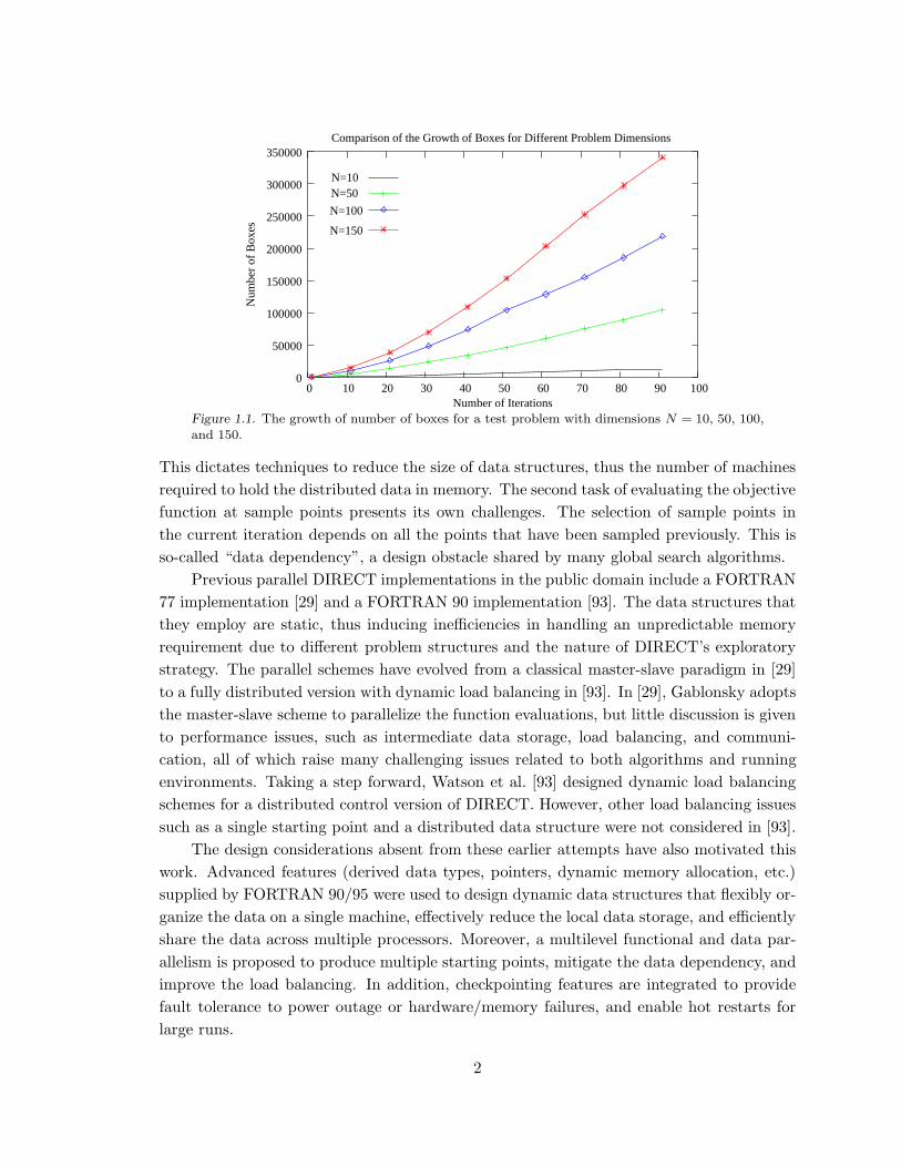
Figure 1.1 shows the growth of the number of search subregions (“boxes”) for a standard
test problem with dimensions N = 10, 50, 100, and 150. The amount of data grows rapidly
as the DIRECT search proceeds in iterations, especially for high dimensional problems.
1
0
50000
100000
150000
200000
250000
300000
350000
0 10 20 30 40 50 60 70 80 90 100
Num
ber
of B
oxes
Number of Iterations
Comparison of the Growth of Boxes for Different Problem Dimensions
N=10N=50
N=100
N=150
Figure 1.1. The growth of number of boxes for a test problem with dimensions N = 10, 50, 100,
and 150.
This dictates techniques to reduce the size of data structures, thus the number of machines
required to hold the distributed data in memory. The second task of evaluating the objective
function at sample points presents its own challenges. The selection of sample points in
the current iteration depends on all the points that have been sampled previously. This is
so-called “data dependency”, a design obstacle shared by many global search algorithms.
Previous parallel DIRECT implementations in the public domain include a FORTRAN
77 implementation [29] and a FORTRAN 90 implementation [93]. The data structures that
they employ are static, thus inducing inefficiencies in handling an unpredictable memory
requirement due to different problem structures and the nature of DIRECT’s exploratory
strategy. The parallel schemes have evolved from a classical master-slave paradigm in [29]
to a fully distributed version with dynamic load balancing in [93]. In [29], Gablonsky adopts
the master-slave scheme to parallelize the function evaluations, but little discussion is given
to performance issues, such as intermediate data storage, load balancing, and communi-
cation, all of which raise many challenging issues related to both algorithms and running
environments. Taking a step forward, Watson et al. [93] designed dynamic load balancing
schemes for a distributed control version of DIRECT. However, other load balancing issues
such as a single starting point and a distributed data structure were not considered in [93].
The design considerations absent from these earlier attempts have also motivated this
work. Advanced features (derived data types, pointers, dynamic memory allocation, etc.)
supplied by FORTRAN 90/95 were used to design dynamic data structures that flexibly or-
ganize the data on a single machine, effectively reduce the local data storage, and efficiently
share the data across multiple processors. Moreover, a multilevel functional and data par-
allelism is proposed to produce multiple starting points, mitigate the data dependency, and
improve the load balancing. In addition, checkpointing features are integrated to provide
fault tolerance to power outage or hardware/memory failures, and enable hot restarts for
large runs.
2

1.2. Research Work Summary
The main goal of this work is to (1) develop an efficient, portable, and robust implementa-
tion of a data-distributed massively parallel DIRECT, (2) evaluate the design effectiveness
on a variety of problems, schemes, and systems, (3) guide the proper choice of optimiza-
tion parameters and application settings, and (4) generalize the design considerations and
analysis techniques that can be applied to parallelizing other global optimization algorithms
challenged by large scale applications on massively parallel systems. A bottom-up approach
was taken to accomplish the goal. The essential building blocks and the corresponding pub-
lications/reports are listed below.
(1) A modified DIRECT algorithm that offers more choices for different types of appli-
cations and preserves its strengths of global convergence and deterministic solution
([49] [50]).
(2) A set of dynamic data structures that adapt to varying memory requirements. ([49])
(3) A memory reduction technique that further mitigates the memory burden. ([46])
(4) Data-distributed massively parallel schemes and portable programming models that
optimize the overall performance on large scale parallel systems. ([41] [40] [46])
(5) Error handling and checkpointing methods to enhance the program robustness. ([50])
(6) Performance studies using modeling and evaluation tools on different types of parallel
systems. ([43] [45] [44])
(7) Real world applications featured with both low and high dimensions. ([42] [48] [47]
[39] [6] [67] [84] [91])
(8) Software documentation on organization and usage that make this work accessible
to others. ([50])
AlgorithmModifications
(1) AlgorithmModifications
(1)
Aug 2000−−Oct 2002M.S. Ph.D.
Oct 2002−−Aug 2007
(7) Applications in Systems Biology
(5) Error handlingand Checkpointing
Dynamic Data Structures
Application in
Wireless Design
(2)
(7)
(3) Memory
Programming ModelsParallel Schemes(4)
Modeling and Analysis(6) Performance
(8)Organization and Usage
Documentation on
Reduction Techniques
Figure 1.2. Research work summary.
3
The M.S. thesis [38] covers most of (1) and (2), and part of (6) and (7), which includes
application examples of DIRECT in wireless communication systems. Several important
improvements were made to the work in [38], so these materials are updated here. Also, a
complete view of the entire body of work is shown in Figure 1.2.
(1) is described in Chapter 2, which also introduces the original DIRECT algorithm
and presents a brief survey of the related work in DIRECT’s modification. (2) and (3)
are discussed in Chapter 3, covering the design issues, efficiency studies, and a survey of
distributed data structures that inspired this work. (4) is presented in Chapter 4, where
two different parallel implementations are compared. Chapter 5 describes (5) and reports
the performance results of the checkpoint method under both serial and parallel computing
environments. Chapter 6 presents (6) for performance study, modeling, and analysis that
were done on System X, a 2200-processor Apple G5 cluster and Anantham, a 400-processor
64-bit Opteron Linux cluster. As examples for (7), real world parameter estimation prob-
lems for cell cycle modeling in systems biology are given in Chapter 7. Appendix A lists all
the artificial test functions used in the study. Finally, (8) is included in Appendix B.
4

CHAPTER 2: The DIRECT Algorithm
Jones et al. [56] invented DIRECT (DIviding-RECTangles) as a Lipschitzian direct
search algorithm for solving global optimization problems (GOPs) subject to bound con-
straints of the form
minx∈D
f(x), (2.1)
where D ={
x ∈ En | ℓ ≤ x ≤ u}
is a bounded box in n-dimensional Euclidean space En,
and f : En → E must satisfy a Lipschitz condition [52]
|f(x1) − f(x2)| ≤ L‖x1 − x2‖, ∀x1, x2 ∈ D. (2.2)
Although DIRECT can be used for local optimization, it was designed as an effective
global method that avoids being trapped at local optima and intelligently explores “poten-
tially optimal” regions to converge globally for Lipschitz continuous optimization problems.
As a direct pattern search method, DIRECT produces deterministic results and is straight-
forward to apply without derivative information or the Lipschitz constant of the objective
function.
2.1. Algorithm
DIRECT’s behavior in multiple dimensions can be viewed as taking steps in potentially
optimal directions within the entire design space. The potentially optimal directions are
determined through evaluating the objective function at center points of the subdivided
boxes. The search is carried out through three essential operations: region selection, point
sampling, and space division. [56] describes the original algorithm in six detailed steps,
which are regrouped and relabeled to highlight the basic operations as below.
Given an objective function f and the feasible set D, the steps are:
1. Initialization. Normalize the feasible set D to be the unit hypercube. Sample
the center point ci of this hypercube and evaluate f(ci). Initialize fmin = f(ci),
evaluation counter m = 1, and iteration counter t = 0.
2. Selection. Identify the set S of “potentially optimal” boxes that are subregions of
D. A box is potentially optimal if, for some Lipschitz constant, the function value
within the box is potentially smaller than that in any other box (a formal definition
with the tuning parameter ǫ is given by [56] and also can be found in [38]; see
Section 3.1 for further explanation of ǫ.)
3. Sampling. For any box j ∈ S, identify the set I of dimensions with the maximum
side length. Let δ equal one-third of this maximum side length. Sample the function
at the points c ± δei for all i ∈ I, where c is the center of the box and ei is the ith
unit vector.
5
−2
−1.5
−1
−0.5
0
0.5
1
1.5
2
−3 −2 −1 0 1 2 3
X2
X1
Six−hump Camel Back Function
(a)
0
2
4
6
8
10
12
14
16
−6 −4 −2 0 2 4 6 8 10
X2
X1
Branin rcos Function
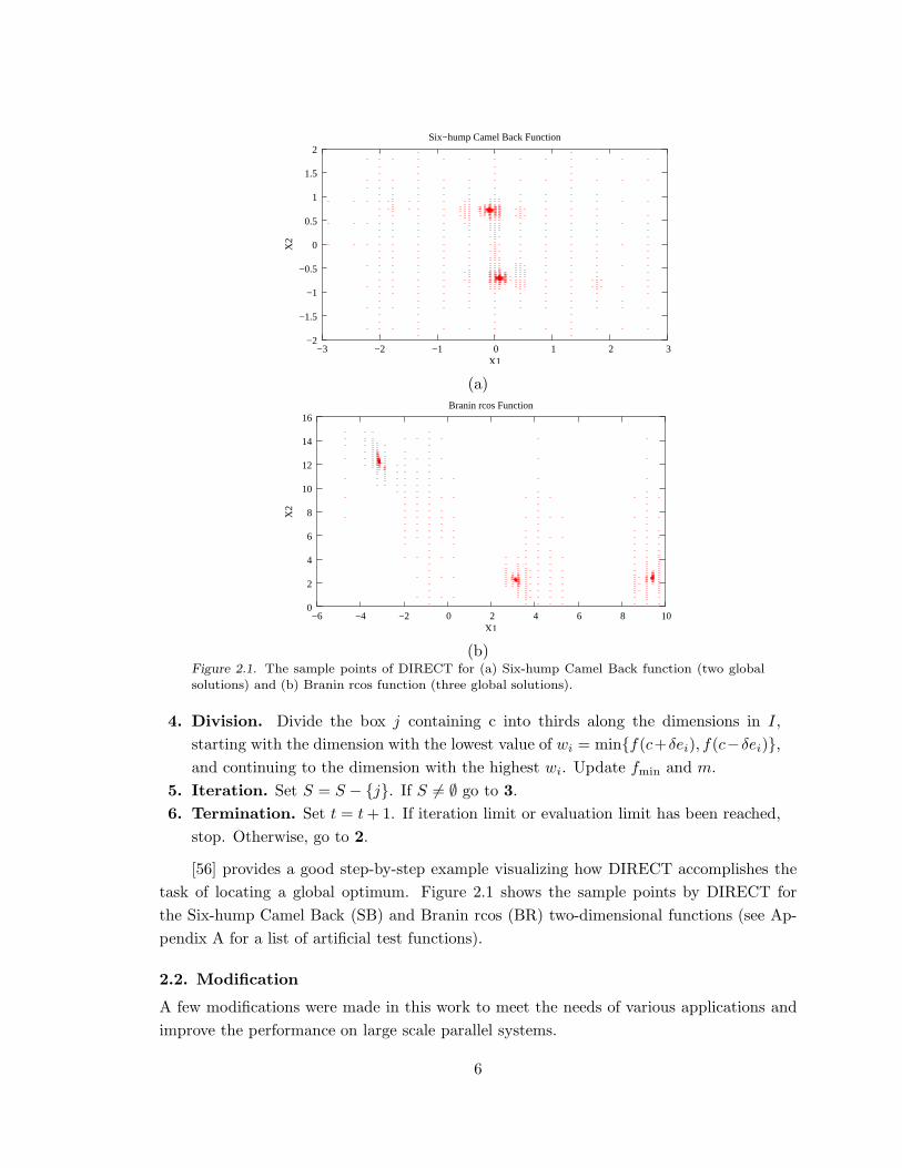
(b)Figure 2.1. The sample points of DIRECT for (a) Six-hump Camel Back function (two global
solutions) and (b) Branin rcos function (three global solutions).
4. Division. Divide the box j containing c into thirds along the dimensions in I,
starting with the dimension with the lowest value of wi = min{f(c+δei), f(c−δei)},and continuing to the dimension with the highest wi. Update fmin and m.
5. Iteration. Set S = S − {j}. If S 6= ∅ go to 3.
6. Termination. Set t = t + 1. If iteration limit or evaluation limit has been reached,
stop. Otherwise, go to 2.
[56] provides a good step-by-step example visualizing how DIRECT accomplishes the
task of locating a global optimum. Figure 2.1 shows the sample points by DIRECT for
the Six-hump Camel Back (SB) and Branin rcos (BR) two-dimensional functions (see Ap-
pendix A for a list of artificial test functions).
2.2. Modification
A few modifications were made in this work to meet the needs of various applications and
improve the performance on large scale parallel systems.
6
For Initialization, an optional domain decomposition step is added to create multiple
subdomains, each with a starting point for a DIRECT search. Empirical results have
shown that this approach significantly improves load balancing among a large number of
processors, and likely shortens the optimization process for problems with asymmetric or
irregular structures.
The second step Selection has two additions. The first is an “aggressive” switch
adopted from [93], which generates more function evaluation tasks that may help balance
the workload under the parallel environment. The second is an adjustable ǫ, which is
recommended by [56] to be within (10−2, 10−7), and “most naturally” 10−4 or the desired
solution accuracy. The studies in [29] [31] show that ǫ = 0.0 speeds up the convergence
for low dimensional problems. In general, smaller ǫ values make the search more local and
generate more function evaluation tasks. On the other hand, larger ǫ values bias the search
toward broader exploration, exhibiting slower convergence. In the present work, the value
of ǫ is taken as zero by default, but can be specified by the user depending on problem
characteristics and optimization goals.
To produce more tasks in parallel, new points are sampled around all boxes in S
along their longest dimensions during Sampling. This modification also removes the step
Iteration, thus simplifying the loop. Differently in the serial version, Sampling samples
one box at a time to eliminate unnecessary storage for new boxes. Another modification
to Sampling is adding lexicographical order comparison between box center coordinates.
Since box center function values may be the same or very close to each other, the parallel
Sampling may yield a different box sequence in each box column as the parallel scheme
varies. As a consequence, boxes will be subdivided in a different order, thus destroying the
deterministic property of DIRECT. Hence, lexicographical order comparison is added to
keep the boxes in the same sampling sequence on the same platform. Unfortunately, the
deterministic property is hard to preserve across machines/compilers that produce different
numerical values, so the numerical results for the same problem may vary slightly on different
systems.
The last set of modifications, in Termination, is to offer more choices of stopping
conditions. [56] commented that the original stopping condition on a limit on iterations
MAX ITER or evaluations MAX EVL is not convincing for many optimization problems. Two
new stopping rules proposed here are (1) minimum diameter MIN DIA (exit when the diam-
eter of the best box has reached the value specified by the user or the round off level) and
(2) objective function convergence tolerance OBJ CONV (exit when the relative change in the
optimum objective function value has reached the given value).
7

2.3. Related Work in DIRECT’s Modification
As a comparatively young method, DIRECT is being enhanced with novel ideas and con-
cepts.
Jones has made a couple of modifications to the original DIRECT[55]. The modified
version in Division only trisects in one dimension with the longest side length instead of
in all identified dimensions in set I as above. The dimension to choose depends upon a tie
breaking mechanism (e.g., random selection or priority by age).
Baker [7] first proposes the “aggressive DIRECT”, which discards the convex hull
idea of identifying potentially optimal boxes. Instead, it subdivides all the boxes with
the smallest objective function values for different box sizes. The change results in more
subdivision tasks generated at every iteration, which helps to balance the workload in a
parallel computing environment.
Ljungberg et al. [61] report that DIRECT performs faster and more accurate than
exhaustive grid search and a genetic algorithm. Zhu et al. [98] also found that DIRECT
converges faster to a global optimum point than adaptive simulated annealing. The secret
may lie in the tuning parameter ǫ defined in DIRECT to balance the global and local search
efforts. Nevertheless, DIRECT still converges slowly compared to local or gradient-based
algorithms, because a significant amount of time is consumed in exploring the entire design
space, which is a common tradeoff between the search broadness and the convergence rate.
Several modifications to DIRECT [29] [31] [28] [82] have been proposed to speed up the
convergence. Gablonsky et al. [31] studied the behavior of DIRECT in low dimensions and
developed an alternative version for biasing the search more toward local improvement by
forcing ǫ = 0. Finkel et al. developed an adaptive restart DIRECT that dynamically checks
the search progress and updates the value of ǫ accordingly. Sergeyev et al. [82] proposed
a diagonal partition strategy which samples two corner points of a region instead of the
center in order to obtain more information about the design space and determine a set of
reasonable Lipschitz constants that accelerate the convergence due to a better balanced
global and local search.
Additionally, combining DIRECT with other methods has been found to be fairly suc-
cessful to address the issue of slow convergence [71] [99] [74]. Nelson et al. [71] incorporated
a trust region step to take advantage of the fast convergence of the local method. For noisy
objective functions, Cox et al. [20] found that a combined local method with DIRECT can
be stalled because it is confined by the bounds of the best box. A strategy called “box
penetration” was developed in [20] to force a subset of boxes neighboring the best box to
divide, thus avoiding being trapped in a local minima. Inside the global search loop of
DIRECT, Zwolak et al. [99] created a local search loop using ODRPACK [14] to refine mul-
tiple sub-optimal results. Panning et al. [74] reported that the combination of DIRECT
and MADS (mesh adaptive direct search) [5] discovered a better point than using either
DIRECT or MADS alone.
8
CHAPTER 3: Data Storage and Sharing
One of the biggest design challenges of DIRECT is to break the “curse of dimensional-
ity” first noted by its creators [56]. The approach here is to design dynamic data structures
that are easily extensible to store continuously generated data from point sampling/space
division and to share the data storage among multiple processors. The original design of
the data structures is reported in [49] and [38], documented for the serial implementation
previously named as VTDIRECT. The design has been improved by adopting a min-heap
data structure and a memory reduction technique, and is used in the latest software package
VTDIRECT95, a Fortran 95 implementation of DIRECT, including both serial and parallel
codes (Appendix B).
3.1. Data Structures
DIRECT keeps subdividing the design space and selects potentially optimal regions accord-
ing to the sampling results. The divided subregions are called “boxes”. The key information
for a box is stored in a derived data type HyperBox, containing an array of center point
coordinates c, an array of box sides side, center point function value val, and box diameter
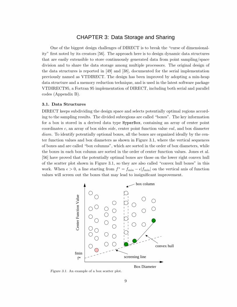
diam. To identify potentially optional boxes, all the boxes are organized ideally by the cen-
ter function values and box diameters as shown in Figure 3.1, where the vertical sequences
of boxes and are called “box columns”, which are sorted in the order of box diameters, while
the boxes in each box column are sorted in the order of center function values. Jones et al.
[56] have proved that the potentially optimal boxes are those on the lower right convex hull
of the scatter plot shown in Figure 3.1, so they are also called “convex hull boxes” in this
work. When ǫ > 0, a line starting from f∗ = fmin − ǫ|fmin| on the vertical axis of function
values will screen out the boxes that may lead to insignificant improvement.
Cen
ter
Fun
ctio
n V
alue
box column
fminf* screening line
convex hull
Box DiameterFigure 3.1. An example of a box scatter plot.
9

The horizontal strict order for the box diameters must be maintained to facilitate the
convex hull computation. However, the vertical strict order of box center function values
(implemented in the serial version described in [49]) is unnecessary for each box column,
and it also incurs more operational cost such as shifting and sorting for box removal and
insertion. Therefore, a min-heap data structure implements a box column, so that the lowest
box owns the smallest function value and every box has a smaller function value than its
left and right children if they exist. It lays out the potentially optimal box candidate at
the bottom of the scatter pattern. Once this candidate box is determined to be potentially
optimal, it will be removed from the heap to be subdivided, and the last box in the heap
will be put to the first position and sifted down, reordering the heap in O(log n) operations
instead of the O(n) shifting operations required by a strictly increasing order of center
function values. Similarly for box insertion, a new box is inserted at the end of the heap
and sifted up in O(log n), reduced from O(n), comparisons. The complexity is improved
considerably, especially for large box columns.
In addition to HyperBox, BoxMatrix and BoxLink are the other two derived data types
for storing boxes. These three are called “box structures” in [49]. BoxMatrix contains the
following components:
(1) a two-dimensional array M of type HyperBox,
(2) an array of box counters ind for box columns,
(3) a pointer child that points to the next linked node of BoxMatrix needed when more
box columns with new diameters are generated,
(4) an array sibling of pointers that point to linked nodes of type BoxLink, which are
used to extend box columns beyond the storage afforded in M, and
(5) id to identify this box matrix among others.
Initially, a box matrix is allocated with empty box column structures (called “free
box columns”) according to the problem dimension and optimization scale. When cur-
rently allocated memory for a box column has been filled up, a new box link of derived
type BoxLink is allocated dynamically adding a one-dimensional array of HyperBoxes and
associated components such as counter, pointers, and ID to extend the box column.
To maintain the strict order of box diameters for box columns, another set of “linked list
structures” organizes box columns and recycles free box columns. The linked lists setFcol
and setInd are of the type int vector, containing a one-dimensional array elements of
integers, an array flags for marking convex hull boxes, pointers for linking nodes, and
the node ID. The array flags is only allocated and used for setInd. The third linked
list setDia is derived from real vector to hold an array of box diameters (real values),
pointers, and ID. When a new box matrix is allocated, all the global IDs of its free box
columns are computed based on its box matrix ID and inserted in setFcol. When a new
box diameter is produced from Division, a free box column from setFcol is assigned to
hold the box. An appropriate position for this box diameter will be found using a binary
10
search in setDia, which is sorted in decreasing order. Then, the global ID of the newly
assigned box column is added in setInd at the corresponding position to that in setDia.
The process is reversed when a box diameter disappears after the last box with this box
diameter has been removed, so this box column becomes free. Subsequently, its diameter
value and the global ID will be taken out from setDia and setInd, respectively. Finally,
the free box column is recycled back to setFcol for later use.
Another practical issue is the sequence of dividing convex hull boxes. Because diameters
are sorted in decreasing order in setDia, the serial version needs to start from the end of
setDia and subdivide the box with the smallest diameter first, so that sifting up newly
generated boxes would not override any existing convex hull boxes. Obviously, this potential
overriding problem does not exist for the parallel version, which buffers all new boxes from
subdivided convex hull boxes and inserts them all at one time. Hence, the parallel version
starts from the beginning of setDia, thus avoiding the unnecessary cost of chasing the
linked nodes of setDia.
A new feature is added to output multiple best boxes (MBB), which are found by
searching through the box structures that hold all the information on the space partition.
This feature is very useful for global optimization problems with complex structures, where
local optimum points are far away from each other, thus demanding a large amount of
space exploration and slowing convergence. In such a case, DIRECT is often used as a
global starter to find good regions. Then, a local optimizer is applied to each region to
efficiently find multiple local optimum points. Examples of this are presented in [99] and
[74]. To activate the MBB option, an empty array BOX SET of type HyperBox allocated
with a user-desired size needs to be specified in the input argument list. Optionally, two
more arguments MIN SEP (minimal separation) and W (weights) can be given to specify the
minimal weighted distance between the center points of the best boxes returned in BOX SET.
By default, MIN SEP is half the diameter of the design space and W is taken as all ones.
When the desired number of best boxes can not be found conditioned on MIN SEP and W,
the output argument NUM BOX is returned as the actual number of best boxes in BOX SET.
The following pseudo code illustrates the MBB process and demonstrates a typical scenario
of manipulating the dynamic data structures.
cc: the current best box center
cb: the counter for best boxes stored in BOX SET
cm: the counter for marked boxes
fmin: minimum function value
fi: the current function value to be compared
i, j, k: loop counters
nb: the desired number of best boxes
nc: the number of columns allocated in M
11

ne: the number of function evaluations
nr: the number of rows allocated in M
pb: the pointer to a box matrix
pc: the pointer to a box
pl: the pointer to a box link
sep: weighted separation between cc and a candidate box
x0: minimizing vector scaled in the original design space
x1: normalized x0 in the unit design space
Store the first best box centered at x0 with value fmin;
Initialize cc and fi
cb := 1
BOX SET(cb)%val := fmin
BOX SET(cb)%c := x0
cc := x1
fi := a very large value
OUTER: do k := 1, nb − 1
Initialize pb to point to the head of box matrices
cm := 0
INNER1: do while (pb is not NULL)
INNER2: do i := 1, nc
INNER3: do j := 1, ((pb%ind(i)-1) mod nr) + 1
Locate the best box with x0 and fmin in the first pass.
if (k = 1) then
if (x1 is the same as pb%M(j, i)%c) then
Found the best box and fill in BOX SET;
Assign the first best box with scaled pb%M(j,i);
Mark off the box at pb%M(j,i);
cm := cm + 1
cycle
end if
end if
if (box at pb%M(j,i) is not marked) then
Compute sep
if (sep < MIN SEP) then
mark off the box at pb%M(j,i)
cm := cm + 1
else
if (box at pb%M(j,i)%val< fi)
12
fi := pb%M(j,i)%val
pc points to the box at pb%M(j,i)
end if
end if
else
cm := cm + 1
end if
end do INNER3
if (any box link exists for this box column) then
pl points to the first box link
do while (pl is not NULL)
Repeat above steps in INNER3 loop for all boxes in pl
pl points to the next box link
end do
end if
end do INNER2
pb points to the next box matrix
end do INNER1
if (pc is not NULL) then
if (pc is not marked) then
Found the next best box at pc; Scale it back to the original design
space and store it in BOX SET
cb := cb + 1
BOX SET(cb) := scaled box at pc
Mark it off
cm := cm + 1
Update cc
cc := pc%c
end if
else
exit OUTER since the next best box is not available
end if
Exit when all evaluated boxes have been marked
if (cm ≥ ne ) exit OUTER
end do OUTER
Pseudocode 3.1.
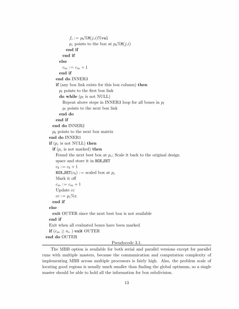
The MBB option is available for both serial and parallel versions except for parallel
runs with multiple masters, because the communication and computation complexity of
implementing MBB across multiple processors is fairly high. Also, the problem scale of
locating good regions is usually much smaller than finding the global optimum, so a single
master should be able to hold all the information for box subdivision.
13

3.2. Memory Reduction Technique
Limiting box columns (LBC) is a technique developed to reduce the memory requirements.
Let Imax (the stopping rule MAX ITER) be the maximum number of iterations allowed (a
stopping criterion), Icurrent be the current iteration number, and C be one of the box
columns. Each of the iterations Icurrent, . . ., Imax can subdivide at most one box from C,
because at most one box from C can be in the set of convex hull boxes at any iteration.
Therefore, C only needs to contain at most L = Imax − Icurrent + 1 boxes with the smallest
function values. Boxes with larger function values are not considered by the DIRECT
search limited to Imax iterations. However, the number of boxes generated per box column
is usually much larger than L. Figure 3.2 shows the box column lengths for (1) the 10-
dimensional Griewank Function (defined in Appendix A) with Imax = 400 and (2) the
143-dimensional budding yeast parameter estimation problem [74] with Imax = 40. Most
of the box columns are longer than Imax >= L in both (1) and (2). When the stopping
criterion Imax is given, storing only L boxes in box columns would significantly reduce the
memory demands.
0
500
1000
1500
2000
2500
3000
3500
4000
4500
0 0.5 1 1.5 2 2.5 3 3.5 4 4.5 5
Num
ber
of b
oxes
Box diameter
box columns
0
100
200
300
400
500
600
700
800
900
1000
0 20 40 60 80 100 120 140
Num
ber
of b
oxes
Box diameter
box columns
Figure 3.2. Box column lengths at the last iteration Imax. (1) The Griewank function (left),N = 10 and Imax = 400. (2) Budding yeast problem (right), N = 143 and Imax = 40.
Since each box column is implemented as a min-heap ordered by the function values at
the box centers, all box column operations without LBC take O(log n) time and only two
types of heap operations are involved—removing the lowest boxes with the smallest function
values and adding new boxes. Additionally, LBC needs to remove the boxes with the largest
function values (bmaxs). The min-heap data structure requires a O(n) time algorithm to
locate the bmax boxes. A min-max heap [4] is considered as an ideal replacement of the min-
heap data structure to locate the bmax boxes with constant time, which makes all operations
O(log n) time. The min-max heap makes a huge difference when Imax is large, since the
number of boxes in a box column heap is very large. Also, several box columns can be taken
into account to further reduce the number of boxes in the memory.
Although the extra operations of removing boxes with the largest function values in
LBC are expensive, the memory requirement is reduced greatly as a result. Therefore, it is
14

highly recommended to enable LBC for large scale/high dimensional problems that more
likely encounter memory allocation failures than small scale/low dimensional problems.
LBC is enabled under three conditions: (1) the specified iteration limit Imax is positive, (2)
the evaluation limit Le (the stopping rule MAX EVL) is not specified or is sufficiently large—
Le × (2N + 2) > 2 × 10⁶, and (3) the MBB option is off. Without Condition (1), LBC
would not be able to decide on the number of boxes to remove. Condition (2) is to turn off
LBC to save operations for small scale runs with little concern for box storage; 2 × 10⁶ is
the threshold obtained from an empirical study. The last condition is also necessary since
the MBB process demands that all boxes stay in the memory.
3.3. Efficiency Study
In terms of the execution time and memory usage, two other implementations ([29] and
[93]) using static data structures were compared empirically with the serial version de-
scribed in [49], which has demonstrated its strength in dealing with unpredictable memory
requirements. The new improvement on data structures here is constructing box columns
as heaps instead of sorted lists. In addition, lexicographical order of box center coordinates
is enforced in the heap for maintaining determinism. Table 3.1 compares the execution
time of an earlier version with sorted lists (SL), the current version with lexicographically
ordered heaps (HL), and a version (HNL) that was built without the lexicographical order
comparisons. Clearly, using heaps is much more efficient than using sorted lists. Also, the
lexicographical order comparison accounts for a very tiny portion of the entire operational
cost.
Table 3.1. Execution time (in seconds) of the versions with sorted lists (SL), with lexicograph-
ically ordered heaps (HL), and heaps without lexicographical order comparison (HNL). The
evaluation limit is 105 for all test functions.
# SL HL HNL
GR 233.21 10.60 10.57QU 840.43 56.70 56.38RO 226.52 8.12 7.92SC 273.58 11.97 11.86MI 468.65 29.69 29.32
The last important improvement on data structures is limiting box columns (LBC).
The experimental results in Section 6.1.3 show that LBC reduces the memory usage by 10–
70% for selected high dimensional test problems. The following experiments investigate the
added computational cost of LBC. Figure 3.3 compares the growth of the execution time
15

0
100
200
300
400
500
600
700
800
900
150000 200000 250000 300000 350000 400000 450000 500000
Tim
e (s
ec.)
LBC vs. NON−LBC for the GR (N=2) and RO (N=4) problems
RO LBCRO NON−LBC
GR NON−LBCGR LBC
Function EvaluationsFigure 3.3. Growth of execution time with LBC or NON-LBC as Ne increases for the 2-
dimensional problem GR and the 4-dimensional problem RO.
with LBC or without LBC (NON-LBC) as the number of function evaluations Ne increases
for the 2-dimensional problem GR and 4-dimensional problem RO.
Regardless of the different problem structures, LBC performs slower than NON-LBC
until Ne reaches a certain “crossover point”, where NON-LBC begins to run slower due to
less memory resource and more expensive operations on the lengthy box columns than LBC,
which keeps the box columns as short as necessary. Observe that the crossover point for the
2-dimensional problem GR is approximately twice the crossover point for the 4-dimensional
problem RO. This observation inspired the next set of experiments to find the approximate
number of evaluations Nx at the crossover points for all five benchmark functions, and
define a condition to turn off LBC if
Le(2N + 2) < Lx, (3.1)
where N is the problem dimension, 2N + 2 is the number of real values in a Hyperbox,
Le is the user specified limit on evaluations, and Lx ≈ 2 × 10⁶ is the average of the five
Nx(2N + 2) values shown in Table 3.2. The condition (3.1) is checked only when the user
specifies both stopping conditions MAX ITER and MAX EVL.
Table 3.2. The crossover point Nx and the threshold Lx for all five test functions.
# GR QU RO SC MI
N 2 3 4 2 5Nx/103 422 190 258 442 129Lx/106 2.5 1.5 2.5 2.6 1.5
16
3.4. Related Work in Distributed Data Structures
Fundamental research on data structures contributed greatly to the design of distributed
data structures used in parallel computing. This section presents a brief survey of several
design examples related to this work.
The first example is octree, a three-dimensional variant of the quadtree with 23 branches
[83]. Some octree-based methods for recursive decomposition of 3-D objects are frequently
used in the construction of meshes for finite element analysis [81]. Pombo et al. [78] intro-
duce adaptive schemes to improve the convergence rate of finite element methods. Parallel
meshing avoids the computation bottlenecks, and therefore solves large-scale problems with
a reasonable amount of time. The research work focuses on fast generation of tetrahe-
dral unstructured meshes in parallel over geometric models with given refinement criteria.
The meshing adaptation strategy not only automates computational methods for numerical
simulations in a discrete domain, but also uses octrees to partition the geometric model
and divide the workload among the processors with little overhead. The octree-based data
structures maintain a hierarchical storage of the information needed in the meshing process.
Thus, searching operations across large data arrays can be avoided mostly. Some special
features of the octree also benefit the parallel implementations of data distribution algo-
rithms. For example, spatial coordinates and level-tags that represent the desired depth in
the branches of the octree in certain locations are stored as control points for conducting
the desired mesh refinement. A weakness of this strategy, as the authors pointed out, is the
load unbalance, a penalty to reduce the cost of subtree migration, which requires complex
trace information for the octree-based data structures.
The second example is k-d tree, a multidimensional spatial data structure for organizing
point data [81], where k denotes the dimensionality of the space being represented. Basically,
it is a binary search tree with the distinction that at each level, a different attribute value
is tested to determine the direction of branching. Its extension has been used in multi-
dimensional searching in a distributed computing environment, as in [70] and [2]. Al-furaih
et al. [2] study efficient parallel constructions of k-d trees on coarse-grained distributed
memory parallel computers. The authors limit their studies to partial tree constructions up
to a specified number of levels for the targeted applications, such as graph partitions and
databases. Thus, a tree construction consists of two phases: a global construction of the first
log p levels in parallel, followed by local sequential tree constructions. For both phases, three
methods are discussed: median-based, sort-based, and bucket-based methods. The global
construction requires distributing data structures among the processors. This generates
collective communication structures. Different approaches taken by these two construction
phases affect the cost of data movements involved in the inter-processor communication.
Both theoretical and experimental analysis on different strategies are given to support the
conclusion that using data parallelism up to log p levels of the tree followed by running
17
the tasks sequentially on each processor is preferable to using task parallelism for large
granularity.
Unlike Al-furaih et al. [2], Nardelli et al. [70] concentrate on research work for im-
proving the scalability of the k-d tree structures as new points are inserted dynamically.
A new performance measure, distribution efficiency, was introduced to provide a means of
comparing different distributed data structures. A brief literature review on the scalable
distributed data structures is also given, covering from one-dimensional structures, such as
distributed linear hashing and order-preserving data structures, to multidimensional ones
like distributed random tree (DRT), B-trees, and R-trees. Here, k-d trees are used in the
support of distributed exact, partial, and range search queries. The system consists of
servers and clients. Each server manages a bucket of data for a leaf of the k-d tree. A set of
“buckets” is a partition of the whole k-d space. Clients have two tasks, one for adding k-d
points to certain buckets, the other for querying the structure. Data structures with dimen-
sion indices are used in both client and server sites to reduce multicast. Experimental results
prove that compared with other data structures, the proposed data structure improves the
efficiency of data management and querying operations on a set of multi-dimensional points
in a distributed framework. In future work, the authors will extend the data structure to
support dynamic point deletions.
18
CHAPTER 4: Parallel Schemes
The functional flow of DIRECT exposes its inherent sequential nature as seen in Chap-
ter 2. The data dependency among the algorithm steps suggests a multilevel parallelism
for Selection and Sampling. The parallel scheme for Selection concentrates on dis-
tributing data among multiple masters to share the memory burden. Several studies [1] [9]
have shown that an appropriate configuration of multiple masters can improve the over-
all performance. Moreover, the data-distributed scheme naturally parallelizes the convex
hull computation by merging multiple local convex hulls to a global one. Differently for
Sampling, a functional parallelism distributes function evaluation tasks to workers. Nev-
ertheless, function evaluations should be computed locally on masters if the evaluation cost
is cheaper than the communication round trip cost. This is called the “horizontal scheme”
(multiple masters without workers) to contrast with the “vertical scheme” (one master and
multiple workers). These two basic schemes are conceptually described as above, but the
underlying implementation can vary greatly depending on the chosen programming models
and inter-processor communication patterns. Section 4.1 discusses how the overall parallel
scheme has evolved from the version pDIRECT I to the version pDIRECT II. Section 4.2
compares the performance of these two versions. A survey of the related work in designing
parallel schemes for well-known global optimization algorithms is in Section 4.3.
4.1. Implementation Evolution
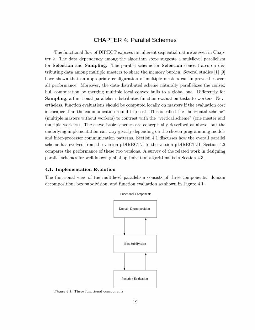
The functional view of the multilevel parallelism consists of three components: domain
decomposition, box subdivision, and function evaluation as shown in Figure 4.1.
Function Evaluation
Domain Decomposition
Box Subdivision
Functional Components
Figure 4.1. Three functional components.
19
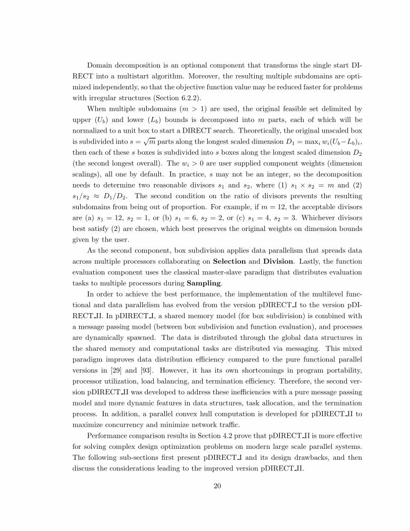
Domain decomposition is an optional component that transforms the single start DI-
RECT into a multistart algorithm. Moreover, the resulting multiple subdomains are opti-
mized independently, so that the objective function value may be reduced faster for problems
with irregular structures (Section 6.2.2).
When multiple subdomains (m > 1) are used, the original feasible set delimited by
upper (Ub) and lower (Lb) bounds is decomposed into m parts, each of which will be
normalized to a unit box to start a DIRECT search. Theoretically, the original unscaled box
is subdivided into s =√
m parts along the longest scaled dimension D1 = maxi wi(Ub−Lb)i,
then each of these s boxes is subdivided into s boxes along the longest scaled dimension D2
(the second longest overall). The wi > 0 are user supplied component weights (dimension
scalings), all one by default. In practice, s may not be an integer, so the decomposition
needs to determine two reasonable divisors s1 and s2, where (1) s1 × s2 = m and (2)
s1/s2 ≈ D1/D2. The second condition on the ratio of divisors prevents the resulting
subdomains from being out of proportion. For example, if m = 12, the acceptable divisors
are (a) s1 = 12, s2 = 1, or (b) s1 = 6, s2 = 2, or (c) s1 = 4, s2 = 3. Whichever divisors
best satisfy (2) are chosen, which best preserves the original weights on dimension bounds
given by the user.
As the second component, box subdivision applies data parallelism that spreads data
across multiple processors collaborating on Selection and Division. Lastly, the function
evaluation component uses the classical master-slave paradigm that distributes evaluation
tasks to multiple processors during Sampling.
In order to achieve the best performance, the implementation of the multilevel func-
tional and data parallelism has evolved from the version pDIRECT I to the version pDI-
RECT II. In pDIRECT I, a shared memory model (for box subdivision) is combined with
a message passing model (between box subdivision and function evaluation), and processes
are dynamically spawned. The data is distributed through the global data structures in
the shared memory and computational tasks are distributed via messaging. This mixed
paradigm improves data distribution efficiency compared to the pure functional parallel
versions in [29] and [93]. However, it has its own shortcomings in program portability,
processor utilization, load balancing, and termination efficiency. Therefore, the second ver-
sion pDIRECT II was developed to address these inefficiencies with a pure message passing
model and more dynamic features in data structures, task allocation, and the termination
process. In addition, a parallel convex hull computation is developed for pDIRECT II to
maximize concurrency and minimize network traffic.
Performance comparison results in Section 4.2 prove that pDIRECT II is more effective
for solving complex design optimization problems on modern large scale parallel systems.
The following sub-sections first present pDIRECT I and its design drawbacks, and then
discuss the considerations leading to the improved version pDIRECT II.
20
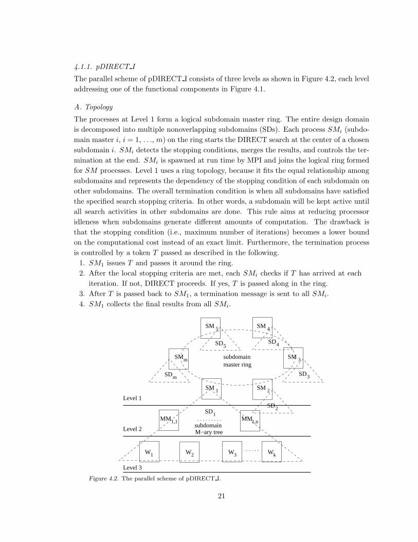
4.1.1. pDIRECT I
The parallel scheme of pDIRECT I consists of three levels as shown in Figure 4.2, each level
addressing one of the functional components in Figure 4.1.
A. Topology
The processes at Level 1 form a logical subdomain master ring. The entire design domain
is decomposed into multiple nonoverlapping subdomains (SDs). Each process SMi (subdo-
main master i, i = 1, . . ., m) on the ring starts the DIRECT search at the center of a chosen
subdomain i. SMi detects the stopping conditions, merges the results, and controls the ter-
mination at the end. SMi is spawned at run time by MPI and joins the logical ring formed
for SM processes. Level 1 uses a ring topology, because it fits the equal relationship among
subdomains and represents the dependency of the stopping condition of each subdomain on
other subdomains. The overall termination condition is when all subdomains have satisfied
the specified search stopping criteria. In other words, a subdomain will be kept active until
all search activities in other subdomains are done. This rule aims at reducing processor
idleness when subdomains generate different amounts of computation. The drawback is
that the stopping condition (i.e., maximum number of iterations) becomes a lower bound
on the computational cost instead of an exact limit. Furthermore, the termination process
is controlled by a token T passed as described in the following.
1. SM1 issues T and passes it around the ring.
2. After the local stopping criteria are met, each SMi checks if T has arrived at each
iteration. If not, DIRECT proceeds. If yes, T is passed along in the ring.
3. After T is passed back to SM1, a termination message is sent to all SMi.
4. SM1 collects the final results from all SMi.
SM
SM
MM
Level 3
Level 2
Level 1
subdomainmaster ring
SM
SM
SMSM
M−ary treesubdomain
MM
1
m
W1
1,1
SD5SD4
SD3
SD2
SDm
SD1
2
3
45
W W W2 3 k
1,n
Figure 4.2. The parallel scheme of pDIRECT I.
21

This process decentralizes the termination control, thus avoiding the bottleneck at
SM1 when the number of subdomains m is large. On the other hand, there are a few
disadvantages of using the ring. First, the communication latency on a ring is higher than
on some other topologies, such as a star or a tree. Second, the lower bound stopping
condition can not provide users accurate estimates of computational cost.
Below Level 1, Level 2 uses GPSHMEM [75] to establish a global addressing space
to access the data for Selection. This globally shared data structure corresponds to a
work pool paradigm [33] that dynamically adjusts box subdivision workload among mini
subdomain master (MM) processes at Level 2. Between Levels 2 and 3, a master-slave
paradigm is used for distributing function evaluation tasks. Both Levels 2 and 3 take
advantage of dynamic process management in MPI-2 [36] so that processors are assigned
to these two levels at run time with approximately (p−m)/m processors available for each
subdomain (out of p total processors). In Figure 4.2, a ⌊M⌋-ary tree structure is rooted at
each SM process, where
M =
√
p − m
m.
Each SM process dynamically spawns n = ⌊M⌋ mini subdomain master (MM) processes
at Level 2 for box subdivision tasks. Similarly, each MM process spawns ⌊k⌋ or ⌈k⌉ worker
processes for function evaluation tasks, where
k =p − m(1 + ⌊M⌋)
m⌊M⌋ .
To form the ⌊M⌋-ary tree of processes, pDIRECT I requires that the total number of
processes P ≥ 16. If the number of available processors p ≥ 16, then P = p. Otherwise, P
is set at 16, so that multiple processes may run on the same physical processor. Pseudocode
4.1 shows the interactions between MMi,1 and MMi,j (j = 2, . . . , n) in subdomain i (i =
1, . . . ,m) managed by SMi.
done := FALSE (the search status)
MMi,1 receives DIRECT parameters (problem size N , domain D,
and stopping conditions Cstop) from SMi
broadcast DIRECT parameters to MMi,j
do
if (MMi,1) then
if (done = FALSE) then
run one DIRECT iteration and merge intermediate results
if (Cstop satisfied) then
done := TRUE
send done to SMi
22
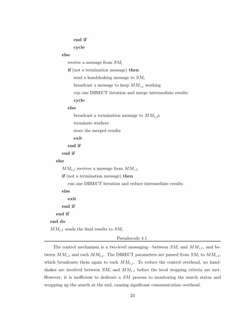
end if
cycle
else
receive a message from SMi
if (not a termination message) then
send a handshaking message to SMi
broadcast a message to keep MMi,j working
run one DIRECT iteration and merge intermediate results
cycle
else
broadcast a termination message to MMi,js
terminate workers
store the merged results
exit
end if
end if
else
MMi,j receives a message from MMi,1
if (not a termination message) then
run one DIRECT iteration and reduce intermediate results
else
exit
end if
end if
end do
MMi,1 sends the final results to SMi
Pseudocode 4.1.
The control mechanism is a two-level messaging—between SMi and MMi,1, and be-
tween MMi,1 and each MMi,j . The DIRECT parameters are passed from SMi to MMi,1,
which broadcasts them again to each MMi,j . To reduce the control overhead, no hand-
shakes are involved between SMi and MMi,1 before the local stopping criteria are met.
However, it is inefficient to dedicate a SM process to monitoring the search status and
wrapping up the search at the end, causing significant communication overhead.
23
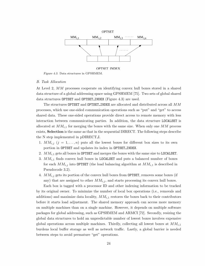
OPTSET_INDEX
MM MM MM MM
OPTSET
i,1 i,2 i,3 i,n
Figure 4.3. Data structures in GPSHMEM.
B. Task Allocation
At Level 2, MM processes cooperate on identifying convex hull boxes stored in a shared
data structure of a global addressing space using GPSHMEM [75]. Two sets of global shared
data structures OPTSET and OPTSET INDEX (Figure 4.3) are used.
The structures OPTSET and OPTSET INDEX are allocated and distributed across all MM
processes, which use one-sided communication operations such as “put” and “get” to access
shared data. These one-sided operations provide direct access to remote memory with less
interaction between communicating parties. In addition, the data structure LOCALSET is
allocated at MMi,1 for merging the boxes with the same size. When only one MM process
exists, Selection is the same as that in the sequential DIRECT. The following steps describe
the N step implemented in pDIRECT I.
1. MMi,j (j = 1, . . . , n) puts all the lowest boxes for different box sizes to its own
portion in OPTSET and updates its index in OPTSET INDEX.
2. MMi,1 gets all boxes in OPTSET and merges the boxes with the same size to LOCALSET.
3. MMi,1 finds convex hull boxes in LOCALSET and puts a balanced number of boxes
for each MMi,j into OPTSET (the load balancing algorithm at MMi,1 is described in
Pseudocode 3.2).
4. MMi,j gets its portion of the convex hull boxes from OPTSET, removes some boxes (if
any) that are assigned to other MMi,j , and starts processing its convex hull boxes.
Each box is tagged with a processor ID and other indexing information to be tracked
by its original owner. To minimize the number of local box operations (i.e., removals and
additions) and maximize data locality, MMi,1 restores the boxes back to their contributors
before it starts load adjustment. The shared memory approach can access more memory
on multiple machines than on a single machine. However, it depends on multiple software
packages for global addressing, such as GPSHMEM and ARMCI [72]. Secondly, resizing the
global data structures to hold an unpredictable number of lowest boxes involves expensive
global operations across multiple machines. Thirdly, collecting all lowest boxes at MMi,1
burdens local buffer storage as well as network traffic. Lastly, a global barrier is needed
between steps to avoid premature “get” operations.
24

Nbox: the number of global convex hull boxesn: the number of MM processesavgload: the average workload measured in boxesunderload: the workload shortfall from the desired avgloadoverload: the workload extra over the desired avgload
merge all boxes from OPTSET to LOCALSET by the box sizesfind convex hull boxes in LOCALSET and update Nbox
restore boxes given by MMi,j to its portion in OPTSET
avgload := ⌈(Nbox/n)⌉d := 1 (loop counter)OUTLOOP: do
if (d = n) exit OUTLOOPif (OPTSET INDEX(d) < avgload) then
d1 := dINLOOP: do
underload := avgload − OPTSET INDEX(d)d1 := (d1) mod nif (d1 = d) exit INLOOPif (OPTSET INDEX(d1) > avgload) then
overload := OPTSET INDEX(d1) − avgloadif (overload ≥ underload) then
shift enough load overOPTSET INDEX(d) := avgloadOPTSET INDEX(d1) := OPTSET INDEX(d1) − underloadexit INLOOP
else
shift some and look for moreOPTSET INDEX(d) := OPTSET INDEX(d) + overloadOPTSET INDEX(d1) := avgload
end if
end if
end do INLOOPend if
d := d + 1end do OUTLOOP
Pseudocode 4.2.
As shown in Pseudocode 4.2, the load adjustment is done at MMi,1, which distributesthe work to MMi,j by using the shared data structures in GPSHMEM. Then, each MMprocess subdivides its share of convex hull boxes and distributes the function evaluationtasks down to its workers. Although the control mechanism is simple, this centralizedstrategy suffers a common bottleneck problem. Furthermore, workers are not shared byMM processes. A worker is exclusively under the command of a particular MM thatspawns it at the beginning. This fixed assignment degrades the processor utilization andload balancing among workers.
25

4.1.2. pDIRECT II
The three-level hierarchy in pDIRECT I is reshaped to be a group-pool structure with sub-
domain groups of masters and a globally shared pool of workers as shown in Figure 4.4.
The SM and MM processes in pDIRECT I are now grouped together to maintain data
structures and perform Selection and Division, while globally shared workers perform
Sampling. This scheme is implemented with a pure message passing model, which re-
moves the dependency on multiple software packages, simplifies the program structure, and
improves the parallel performance.
SD
SD SD
SD
global worker pool
1
SM
SM
1,1
SM 1,n1,22
SM2,1
m
SMm,1
3 SM3,1
masterssubdomain
workersW1 W2 W3 Wk
Figure 4.4. The parallel scheme for pDIRECT II.
A. Topology
Each subdomain is served by a subdomain group of masters in lieu of the subdomain
master ring. Let SMi,j stand for the master j in subdomain i. SMi,1 is the root master
for subdomain i. In addition to carrying out common tasks like other masters, the root
masters SMi,1 (i = 2, . . . ,m) also communicate with SM1,1 to finalize the search. This star
shaped connection centered at SM1,1 has replaced the ring topology in pDIRECT I.
Moreover, all SMi,j (j = 1, . . ., n) processes except SM1,1 become workers when
they have finished all search activities for their subdomain. This dynamic feature reduces
the processor idleness and offers an exact stopping condition unavailable in pDIRECT I.
When the stopping condition is satisfied, workers will receive “all done” messages from
26
masters and terminate themselves after confirming that no more work is available. Then,
a termination message is sent from the root master (processor 0) down to a logical tree of
master processors in log2(n×m) steps, where n×m is the total number of masters. Recall
that the termination message is passed linearly along the ring and logarithmically down
to the ⌊M⌋-ary trees in pDIRECT I. Clearly, the new termination scheme here does not
require such a complicated control mechanism as in pDIRECT I.
B. Task Allocation
Task allocation policies have strong connections to important performance metrics such as
parallel efficiency and load balancing. Here, several improvements were made in allocating
both box subdivision tasks in the Selection step and function evaluation tasks in the
Sampling step.
In subdomain i, Selection is accomplished jointly by masters SMi,j , j = 1, . . ., n,
where n is the total number of subdomain masters per subdomain. When n = 1, Selection
is the same as that in the sequential DIRECT. When n > 1, Selection is done in parallel
over the index i as follows.
1. SMi,j , j = 1, . . . , n identify local convex hull box sets Si,j, j = 1, . . ., n.
2. SMi,1 gathers the Si,j from all the SMi,j .
3. SMi,1 merges the Si,j by box diameters and finds the global convex hull box set Si.
4. All the SMi,j receive the global set Si and find their portion of the convex hull boxes.
All buffers used here are locally allocated and resized incrementally according to the
updated number of boxes involved in the convex hull computation. Note that all boxes
in the global convex hull box set Si must also be in the union of the sets of local convex
hull boxes (Si,j) of the masters. Therefore, each master SMi,j computes Si,j in parallel
and SMi,1 only considers the union of all Si,j instead of all the lowest boxes with different
diameters, as was done in pDIRECT I. This decentralized Selection implementation re-
duces memory requirements for buffers, as well as the amount of data transferred over the
network. However, a large number of subdomain masters will not perform well due to the
global communication and synchronization required for finding convex hull boxes at every
iteration. [97] describes a sampling technique that can further reduce the bandwidth re-
quirements, but it comes at the expense of requiring another global communication round.
Another possibility would be for SMi,1 to gather via a d-way tree only the final merged Si,j ,
where each intermediate tree node does a partial convex hull merge of its d (merged) inputs
(the optimal value for d is derived in [97]). Depending on the potential memory require-
ment of a run, users can estimate the number of subdomain masters required to achieve
a particular stopping condition. If the function evaluation cost is high, but the memory
requirement is hard to assess, the checkpointing feature can be enabled to log evaluations
27

boxes boxes boxes
SMi,1 SMi,2 SMi,3 SMi,n
(a) Horizontal 1-D partition.
function evaluations
WORKER POOL
SMi,j
W1 W2 W3 Wk
(b) Vertical 1-D partition.Figure 4.5. Task partition schemes.
on existing masters and recover the run with more masters if memory allocation failure
occurs.
Compared to pDIRECT I, pDIRECT II simplifies the implementation of the two ba-
sic schemes of task partitioning, namely the horizontal and vertical schemes. As discussed
previously, for low computation cost, communication overhead dominates the parallel execu-
tion time and overshadows the benefits in distributing function evaluation tasks to workers.
Wisely, masters would rather keep computation locally and simply share the memory bur-
den with other masters without any worker involved in the picture. This is the horizontal
scheme, also called horizontal 1-D partition for box subdivision tasks (Figure 4.5(a)). Ex-
perimental results in Section 4.2 show that this scheme achieves better speedup (for cheap
function evaluations) than the vertical 1-D partition (the vertical scheme) for function eval-
uation tasks (shown in Figure 4.5(b)).
When these two schemes are combined, they become a hybrid 2-D partition. This
hybrid scheme is usually preferred for the following reasons. First, the computation cost is
higher or at least comparable to the communication cost in most real world design problems.
Generally, overlapping the computation on worker processors in the vertical 1-D partition
is a reasonable approach. Second, the data sharing scheme in the horizontal 1-D partition
relieves the heavy memory burden on a single master processor for solving a large scale
and/or high dimensional problem.
The next improved design in task allocation is on worker assignment. The worker pool
is globally shared by all masters in all subdomain groups. Each worker polls all (selected)
masters for evaluation tasks and returns the function values. Workers proceed in cycles that
roughly correspond to the DIRECT iterations. During each cycle, a worker requests tasks
from a randomly selected subset of masters until all of them are out of work. This is called
28

the “nonblocking” loop in Pseudocode 4.3. Once the cycle is over, the worker blocks waiting
(the “blocking” loop) for further instructions from a fixed master, which is selected such
that every master has a fair number of blocked workers waiting in the queue. Pseudocode
4.3 below describes how a worker Wi evaluates the objective function for masters SMi,j
(i = 1, . . ., m and j = 1, . . ., n) during Sampling.
Cactive: the counter for the total number of “active” masters
that have not reached the last iteration
Cidle: the counter for idle masters
converted: the flag indicating if it is converted from a master
loop: the loop status
m: the number of subdomains, given as input
n: the number of masters per subdomain, given as input
mesg: the message received from others
Pwi: the processor ID (PID) of Wi
subs: completion statuses of subdomains, given as input
loop := “nonblocking”
converted :=FALSE
Cactive := 0
check subs to compute Cactive
if (Cactive < nm) converted := TRUE
Cidle := 0 (assume all masters busy initially)
OUTLOOP: do
if (loop = “nonblocking”) then
send a nonblocking request to a randomly selected master SMi,j
from Cactive − Cidle busy masters
else
set all masters to status busy
Cidle := 0
send a blocking request to the master SMi,j that ranks as
(Pwi − Cactive) mod Cactive in the list of all active masters
end if
INLOOP: do
keep waiting for any messages
select case (mesg)
case (an evaluation task from SMi,j)
evaluate all points in the task
send the results back to SMi,j
29

if (SMi,j is responding to a blocking request) then
loop := “nonblocking”
end if
case (“no point” from SMi,j)
if (SMi,j is at status busy) then
set SMi,j ’s status idle
Cidle := Cidle + 1
end if
exit INLOOP
case (“all done” from SMi,j)
if (SMi,j is at status busy) then
set SMi,j ’s status idle
Cidle := Cidle + 1
end if
remove SMi,j from the master list
Cactive := Cactive − 1
if (Cactive = 0) then
if (NOT converted)
exit OUTLOOP (terminate itself)
else
cycle INNER (wait for “terminate”)
end if
end if
exit INLOOP
case (a “non-blocking” request from a worker)
reply “all done” to this worker (Wi was converted from a master)
case (a “blocking” request from a worker)
reply “all done” to this worker (Wi was converted from a master)
case (“terminate” from the parent processor)
pass “terminate” to the left and right children (if any)
exit OUTLOOP
end select case
end do INLOOP
if (Cactive = Cidle) then
loop := “blocking”
else
loop := “nonblocking”
end if
30
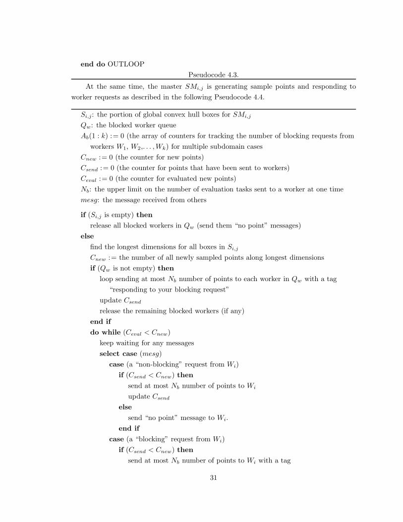
end do OUTLOOP
Pseudocode 4.3.
At the same time, the master SMi,j is generating sample points and responding to
worker requests as described in the following Pseudocode 4.4.
Si,j: the portion of global convex hull boxes for SMi,j
Qw: the blocked worker queue
Ab(1 : k) := 0 (the array of counters for tracking the number of blocking requests from
workers W1, W2,. . . ,Wk) for multiple subdomain cases
Cnew := 0 (the counter for new points)
Csend := 0 (the counter for points that have been sent to workers)
Ceval := 0 (the counter for evaluated new points)
Nb: the upper limit on the number of evaluation tasks sent to a worker at one time
mesg: the message received from others
if (Si,j is empty) then
release all blocked workers in Qw (send them “no point” messages)
else
find the longest dimensions for all boxes in Si,j
Cnew := the number of all newly sampled points along longest dimensions
if (Qw is not empty) then
loop sending at most Nb number of points to each worker in Qw with a tag
“responding to your blocking request”
update Csend
release the remaining blocked workers (if any)
end if
do while (Ceval < Cnew)
keep waiting for any messages
select case (mesg)
case (a “non-blocking” request from Wi)
if (Csend < Cnew) then
send at most Nb number of points to Wi
update Csend
else
send “no point” message to Wi.
end if
case (a “blocking” request from Wi)
if (Csend < Cnew) then
send at most Nb number of points to Wi with a tag
31
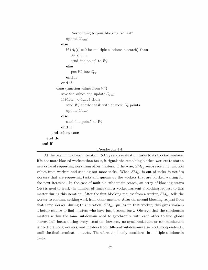
“responding to your blocking request”
update Csend
else
if (Ab(i) = 0 for multiple subdomain search) then
Ab(i) := 1
send “no point” to Wi
else
put Wi into Qw
end if
end if
case (function values from Wi)
save the values and update Ceval
if (Csend < Cnew) then
send Wi another task with at most Nb points
update Csend
else
send “no point” to Wi
end if
end select case
end do
end if
Pseudocode 4.4.
At the beginning of each iteration, SMi,j sends evaluation tasks to its blocked workers.
If it has more blocked workers than tasks, it signals the remaining blocked workers to start a
new cycle of requesting work from other masters. Otherwise, SMi,j keeps receiving function
values from workers and sending out more tasks. When SMi,j is out of tasks, it notifies
workers that are requesting tasks and queues up the workers that are blocked waiting for
the next iteration. In the case of multiple subdomain search, an array of blocking status
(Ab) is used to track the number of times that a worker has sent a blocking request to this
master during this iteration. After the first blocking request from a worker, SMi,j tells the
worker to continue seeking work from other masters. After the second blocking request from
that same worker, during this iteration, SMi,j queues up that worker; this gives workers
a better chance to find masters who have just become busy. Observe that the subdomain
masters within the same subdomain need to synchronize with each other to find global
convex hull boxes during every iteration; however, no synchronization or communication
is needed among workers, and masters from different subdomains also work independently,
until the final termination starts. Therefore, Ab is only considered in multiple subdomain
cases.
32
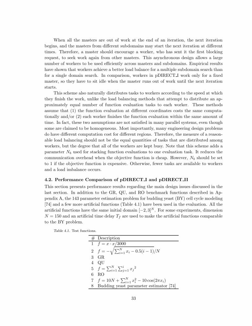
When all the masters are out of work at the end of an iteration, the next iteration
begins, and the masters from different subdomains may start the next iteration at different
times. Therefore, a master should encourage a worker, who has sent it the first blocking
request, to seek work again from other masters. This asynchronous design allows a large
number of workers to be used efficiently across masters and subdomains. Empirical results
have shown that workers achieve a better load balance for a multiple subdomain search than
for a single domain search. In comparison, workers in pDIRECT I work only for a fixed
master, so they have to sit idle when the master runs out of work until the next iteration
starts.
This scheme also naturally distributes tasks to workers according to the speed at which
they finish the work, unlike the load balancing methods that attempt to distribute an ap-
proximately equal number of function evaluation tasks to each worker. These methods
assume that (1) the function evaluation at different coordinates costs the same computa-
tionally and/or (2) each worker finishes the function evaluation within the same amount of
time. In fact, these two assumptions are not satisfied in many parallel systems, even though
some are claimed to be homogeneous. Most importantly, many engineering design problems
do have different computation cost for different regions. Therefore, the measure of a reason-
able load balancing should not be the equal quantities of tasks that are distributed among
workers, but the degree that all of the workers are kept busy. Note that this scheme adds a
parameter Nb used for stacking function evaluations to one evaluation task. It reduces the
communication overhead when the objective function is cheap. However, Nb should be set
to 1 if the objective function is expensive. Otherwise, fewer tasks are available to workers
and a load imbalance occurs.
4.2. Performance Comparison of pDIRECT I and pDIRECT II
This section presents performance results regarding the main design issues discussed in the
last section. In addition to the GR, QU, and RO benchmark functions described in Ap-
pendix A, the 143 parameter estimation problem for budding yeast (BY) cell cycle modeling
[74] and a few more artificial functions (Table 4.1) have been used in the evaluation. All the
artificial functions have the same initial domain [−2, 3]N . For some experiments, dimension
N = 150 and an artificial time delay Tf are used to make the artificial functions comparable
to the BY problem.
Table 4.1. Test functions.
# Description1 f = x · x/3000
2 f = −√
∑N
i=1 xi − 0.5(i − 1)/N
3 GR4 QU
5 f =∑N
i=1
∑i
j=1 xj2
6 RO
7 f = 10N +∑N
i=1 x2i − 10 cos(2πxi)
8 Budding yeast parameter estimator [74]
33

The following experiments demonstrate the effectiveness of the Selection implemen-
tation, task partition, and worker assignment in pDIRECT II.
4.2.1. Selection Efficiency
Table 4.2 compares Ngc (number of global convex hull boxes), Nlc (the combined number
of local convex hull boxes), and Nd (the combined number of different box diameters) on
32 subdomain masters for all test functions at the last iteration (Imax = 1000 for artificial
test functions and Imax = 100 for the budding yeast problem). In pDIRECT I, MMi,1
collects Nd boxes and finds the convex hull box set. In pDIRECT II, Nlc local convex
hull boxes are found by SMi,j (j = 1, . . ., n), then gathered on SMi,1, which identifies
the global convex hull boxes. This approach increases the concurrency of the Selection
implementation. Table 4.2 shows that it reduces the amount of data transferred over the
network and the buffer size by 50–90% for all test functions.
Table 4.2. Comparison of Ngc, Nlc, and Nd at the last iteration Imax.
# Ngc Nlc Nd(Nd−Nlc)
Nd
1 58 2605 33358 92%2 89 1228 6805 81%3 145 2056 22375 90%4 3 3201 6756 52%5 140 1830 20276 90%6 144 1276 28003 95%7 144 3531 20614 82%8 20 159 6545 97%
4.2.2. Task Partition
The following experiment is to study the parallel performance of the horizontal and vertical
1-D partition schemes. A total of P = 288 processors are used. In the horizontal partition,
each run has all P masters that evaluate objective functions locally. In the vertical partition,
a single master sends evaluation tasks to P − 1 workers, each task holding Nb = 1 set of
point coordinates. Table 4.3 shows the timing results for Test Function 6 with N = 150,
given two function evaluation costs: Tf=0.1 second (the artificial case) and the original cost
Tf ≈ 0.0 (less than 1.0E-7 second). Set Imax = 300 for the original cost and Imax = 90
for the artificial cost. To ensure that the two partition schemes are comparable in the
number of processors, the timing results are measured from P = 3 processors (if P = 1, no
workers are used in the vertical 1-D partition). Note that the horizontal 1-D partition has
all P processors available for function evaluations, while the vertical 1-D partition has only
P − 1 processors for that. Therefore, the parallel efficiency is estimated with the base = 3
34

Table 4.3. Parallel timing results (in seconds) for different function evaluation costs Tf for Test
Function 6 with N = 150.
Horizontal 1-D partitionTf\P 3 5 9 18 36 72 144 2880.0 21.04 15.36 12.03 12.78 14.88 40.71 23.37 31.490.1 6785.88 4614.23 2741.11 2633.46 2634.53 2636.03 2652.78 2644.96
Vertical 1-D partitionTf\P 3 5 9 18 36 72 144 2880.0 49.93 41.18 40.28 41.81 45.10 45.53 65.10 55.070.1 8720.27 4361.30 2184.76 1033.28 507.14 256.09 149.95 79.27
0
0.1
0.2
0.3
0.4
0.5
0.6
0.7
0.8
0.9
1
0 50 100 150 200 250 300
Effi
cien
cy
Number of Processors
HP_1VP_1HP_0VP_0
Figure 4.6. Comparison of the parallel efficiencies with different partition schemes and objective
function costs.
processors for the horizontal 1-D partition and base = 2 for the vertical 1-D partition. The
efficiency E is thus computed as (Tbase/TP )/
(P/base) as shown in Figure 4.6.
When Tf = 0.0 second, the horizontal 1-D partition (HP 0) runs faster than the vertical
1-D partition (VP 0). The masters in HP 0 locally evaluate the cheap objective function,
thus avoiding the communication overhead for talking to workers. However, HP 0 does
not achieve any speedup for P = 72, 144, and 288, because the number of convex hull
boxes is insufficient to keep all masters busy (some masters have no convex hull boxes, thus
evaluating no points locally). As for VP 0, the communication overhead always dominates
the execution cost and it fails to achieve any speedup after P reaches 144. When Tf = 0.1
second, the vertical 1-D partition (VP 1) runs more efficiently than the horizontal 1-D
partition (HP 1) (see Figure 4.6) except for P = 3. When P = 3, three masters are
evaluating functions for HP 1, while only two workers are doing so for VP 1. Nevertheless,
all runs with P ≥ 5 of VP 1 take a much shorter time than those of HP 1. The first reason
is that the communication overhead is negligible compared to the objective function cost
35
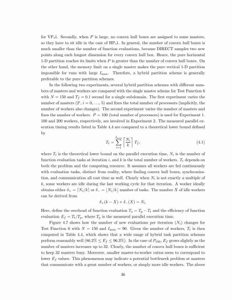
for VP 1. Secondly, when P is large, no convex hull boxes are assigned to some masters,
so they have to sit idle in the case of HP 1. In general, the number of convex hull boxes is
much smaller than the number of function evaluations, because DIRECT samples two new
points along each longest dimension for every convex hull box. Hence, the pure horizontal
1-D partition reaches its limits when P is greater than the number of convex hull boxes. On
the other hand, the memory limit on a single master makes the pure vertical 1-D partition
impossible for runs with large Imax. Therefore, a hybrid partition scheme is generally
preferable to the pure partition schemes.
In the following two experiments, several hybrid partition schemes with different num-
bers of masters and workers are compared with the single master scheme for Test Function 6
with N = 150 and Tf = 0.1 second for a single subdomain. The first experiment varies the
number of masters (2i, i = 0, . . ., 5) and fixes the total number of processors (implicitly, the
number of workers also changes). The second experiment varies the number of masters and
fixes the number of workers. P = 100 (total number of processors) is used for Experiment 1.
100 and 200 workers, respectively, are involved in Experiment 2. The measured parallel ex-
ecution timing results listed in Table 4.4 are compared to a theoretical lower bound defined
by
Tt =
Imax∑
i=1
⌈
Ni
k
⌉
Tf , (4.1)
where Tt is the theoretical lower bound on the parallel execution time, Ni is the number of
function evaluation tasks at iteration i, and k is the total number of workers. Tt depends on
both the problem and the computing resource. It assumes all workers are fed continuously
with evaluation tasks, distinct from reality, where finding convex hull boxes, synchroniza-
tion, and communication all cost time as well. Clearly when Ni is not exactly a multiple of
k, some workers are idle during the last working cycle for that iteration. A worker ideally
obtains either δ+ = ⌈Ni/k⌉ or δ− = ⌊Ni/k⌋ number of tasks. The number X of idle workers
can be derived from
δ+(k − X) + δ−(X) = Ni.
Here, define the overhead of function evaluation To = Tp − Tt and the efficiency of function
evaluation Ef = Tt/Tp, where Tp is the measured parallel execution time.
Figure 4.7 shows how the number of new evaluations per iteration (Ni) changes for
Test Function 6 with N = 150 and Imax = 90. Given the number of workers, Tt is then
computed in Table 4.4, which shows that a wide range of hybrid task partition schemes
perform reasonably well (86.2% ≤ Ef ≤ 96.3%). In the case of P100, Ef grows slightly as the
number of masters increases up to 32. Clearly, the number of convex hull boxes is sufficient
to keep 32 masters busy. Moreover, smaller master-to-worker ratios seem to correspond to
lower Ef values. This phenomenon may indicate a potential bottleneck problem at masters
that communicate with a great number of workers, or simply more idle workers. The above
36

Table 4.4. Comparison of theoretical parallel execution time Tt and the parallel timing results
Tp with different hybrid partition schemes for Test Function 6 with N = 150, Tf = 0.1 sec, and
Imax = 90. P100 stands for using a total of 100 processors. W100, W200 stand for using a total
of 100, 200 workers, respectively.
Number of Mastersschemes 1 2 4 8 16 32
P100 Tp 203.42 204.20 207.79 215.44 234.15 282.38Tt 180.10 181.70 185.80 192.90 211.40 260.20To 23.32 24.10 26.09 29.64 41.25 22.18Ef 88.5% 88.9% 89.4% 89.5% 90.3% 92.1%
W100 Tp 201.53 185.41 184.83 184.88 185.61 187.29Tt 178.00 178.00 178.00 178.00 178.00 178.00To 23.53 7.41 6.83 6.88 7.61 9.29Ef 88.3% 96.0% 96.3% 96.3% 95.9% 95.0%
W200 Tp 102.32 102.06 101.56 101.55 103.14 105.86Tt 91.30 91.30 91.30 91.30 91.30 91.30To 11.02 10.76 10.26 10.25 11.84 14.56Ef 89.2% 89.5% 89.9% 89.9% 88.5% 86.2%
supposition was further investigated in the second experiment. In both W100 and W200, Ef
is improved at the beginning as the number of masters increases to a “peak point” with the
best Ef . Then, it is degraded when the synchronization overhead among masters starts to
dominate. Note that the peak point is 4 for W100 and 8 for W200, while the master-to-worker
ratios at these two points are the same, 1:25. Moreover, W200 has lower Ef values than
W100 for the same number of masters, because masters in W200 deal with more workers, and
more workers in W200 are likely to be idle. Also, the same amount of work distributed to 100
workers in W100 generates more communication interactions between masters and workers
in W200. Therefore, the search with a single subdomain will always eventually decrease Ef
as more and more workers are used.
500
1000
1500
2000
2500
3000
0 10 20 30 40 50 60 70 80 90
New
eva
luat
ions
per
iter
atio
n
Number of Iterations
number of evaluations
Figure 4.7. The plot of Ni (i = 1, . . ., 90) for Test Function 6 with N = 150.
37

4.2.3. Worker Assignment
The following experiment demonstrates that function evaluation tasks are allocated more ef-
ficiently for a multiple subdomain search than for a single subdomain search. Load balancing
among workers is improved greatly with the globally shared worker pool of pDIRECT II, es-
pecially when masters of different subdomains generate unequal amounts of work. P = 320
processors were used for the budding yeast problem. P = 200 processors were used for the
artificial test problems (Test Functions 1–7) with N = 150 and Tf = 0.1 sec.
In this experiment, the feasible domain is split into four subdomains. Note that the
same test problem with four split subdomains can be solved in three different ways using
P processors.
(a) All P processors are used to run a multiple subdomain search with four subdomains.
The parallel execution time is Ta.
(b) Four single subdomain searches are run in parallel, each using P/4 processors on
one of the four subdomains. The overall parallel execution time Tb is the longest
duration of all four runs.
(c) Four single subdomain searches are run sequentially, each using all P processors on
each of the four subdomains. The parallel execution time Tc is the total duration of
these four runs.
Table 4.5. Comparison of Ta, Tb, and Tc in seconds.
# Ta Tb Tc(Tb−Ta)
Ta
(Tc−Ta)Ta
1 382 407 441 6.2% 15.4%2 1132 1139 1185 0.6% 4.6%3 358 369 417 3.1% 16.4%4 870 874 921 0.4% 5.9%5 260 263 312 1.1% 20.0%6 428 476 477 11.2% 11.4%7 1142 1148 1196 0.5% 4.7%8 8595 10643 11059 23.8% 28.7%
Table 4.6. Comparison of total number of subdomain function evaluations for experiments listed
in Table 4.5. ei is the total number of evaluations for subdomain i, which is the same for all of
the ways (a), (b), and (c).
# e1 e2 e3 e4 e s2
1 181409 194927 194927 181463 2090.9 7789.12
2 550691 550691 550691 550691 6118.8 03 176075 176075 176075 176075 1956.4 04 421723 421723 421723 421723 4685.8 05 123685 123685 123685 123685 1374.3 06 228193 203635 198727 192397 2286.0 156612
7 555435 555435 555435 555435 6171.5 08 82471 44631 47531 87063 1635.6 224452
38
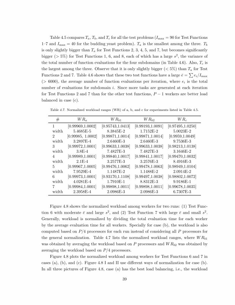
Table 4.5 compares Ta, Tb, and Tc for all the test problems (Imax = 90 for Test Functions
1–7 and Imax = 40 for the budding yeast problem). Ta is the smallest among the three. Tb
is only slightly bigger than Ta for Test Functions 2, 3, 4, 5, and 7, but becomes significantly
bigger (> 5%) for Test Functions 1, 6, and 8, each of which has a large s2, the variance of
the total number of function evaluations for the four subdomains (in Table 4.6). Also, Tc is
the largest among the three. Observe that it is only slightly bigger (< 5%) than Ta for Test
Functions 2 and 7. Table 4.6 shows that these two test functions have a large e =∑
ei/Imax
(> 6000), the average number of function evaluations per iteration, where ei is the total
number of evaluations for subdomain i. Since more tasks are generated at each iteration
for Test Functions 2 and 7 than for the other test functions, P − 1 workers are better load
balanced in case (c).
Table 4.7. Normalized workload ranges (WR) of a, b, and c for experiments listed in Table 4.5.
# WRa WRb1 WRb2 WRc
1 [0.99969,1.0002] [0.95743,1.0413] [0.99193,1.0091] [0.97495,1.0250]width 5.4685E-5 8.3845E-2 1.7152E-2 5.0023E-22 [0.99985, 1.0002] [0.99871,1.0014] [0.99871,1.0014] [0.9959,1.0049]width 3.2897E-4 2.6460E-3 2.6460E-3 9.7536E-33 [0.99972,1.0001] [0.99633,1.0038] [0.99633,1.0038] [0.98213,1.0138]width 3.8E-4 7.4827E-3 7.4827E-3 3.1646E-24 [0.99989,1.0001] [0.99840,1.0017] [0.99841,1.0017] [0.99470,1.0032]width 2.1E-4 3.2577E-3 3.2576E-3 8.4916E-35 [0.99967,1.0005] [0.99476,1.0062] [0.99478,1.0063] [0.98949,1.0104]width 7.9529E-4 1.1487E-2 1.1488E-2 2.0914E-26 [0.99973,1.0001] [0.93170,1.1108] [0.99497,1.0038] [0.98802,1.0072]width 4.0281E-4 1.7910E-1 8.8312E-3 9.9186E-17 [0.99984,1.0001] [0.99898,1.0011] [0.99898,1.0011] [0.99678,1.0035]width 2.3958E-4 2.0986E-3 2.0986E-3 6.7307E-3
Figure 4.8 shows the normalized workload among workers for two runs: (1) Test Func-
tion 6 with moderate e and large s2, and (2) Test Function 7 with large e and small s2.
Generally, workload is normalized by dividing the total evaluation time for each worker
by the average evaluation time for all workers. Specially for case (b), the workload is also
computed based on P/4 processors for each run instead of considering all P processors for
the general normalization. Table 4.7 lists the normalized workload ranges, where WRb1
was obtained by averaging the workload based on P processors and WRb2 was obtained by
averaging the workload based on P/4 processors.
Figure 4.8 plots the normalized workload among workers for Test Functions 6 and 7 in
cases (a), (b), and (c). Figure 4.8 I and II use different ways of normalization for case (b).
In all three pictures of Figure 4.8, case (a) has the best load balancing, i.e., the workload
39
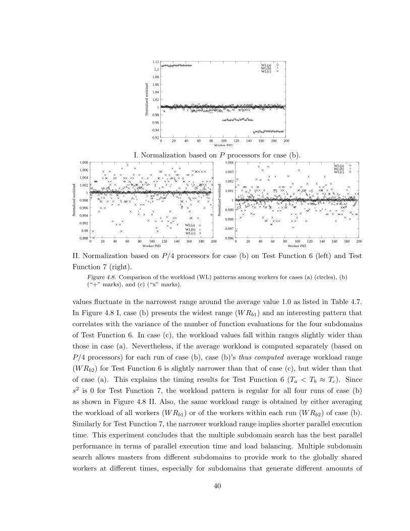
0.92
0.94
0.96
0.98
1
1.02
1.04
1.06
1.08
1.1
1.12
0 20 40 60 80 100 120 140 160 180 200
Nor
mal
ized
wor
kloa
dWorker PID
WL(c)
WL(a)WL(b)
I. Normalization based on P processors for case (b).
0.988
0.99
0.992
0.994
0.996
0.998
1
1.002
1.004
1.006
1.008
0 20 40 60 80 100 120 140 160 180 200
Nor
mal
ized
wor
kloa
d
Worker PID
WL(a)WL(b)WL(c)
0.996
0.997
0.998
0.999
1
1.001
1.002
1.003
1.004
0 20 40 60 80 100 120 140 160 180 200
Nor
mal
ized
wor
kloa
d
Worker PID
WL(a)
WL(c)WL(b)
II. Normalization based on P/4 processors for case (b) on Test Function 6 (left) and Test
Function 7 (right).
Figure 4.8. Comparison of the workload (WL) patterns among workers for cases (a) (circles), (b)(“+” marks), and (c) (“x” marks).
values fluctuate in the narrowest range around the average value 1.0 as listed in Table 4.7.
In Figure 4.8 I, case (b) presents the widest range (WRb1) and an interesting pattern that
correlates with the variance of the number of function evaluations for the four subdomains
of Test Function 6. In case (c), the workload values fall within ranges slightly wider than
those in case (a). Nevertheless, if the average workload is computed separately (based on
P/4 processors) for each run of case (b), case (b)’s thus computed average workload range
(WRb2) for Test Function 6 is slightly narrower than that of case (c), but wider than that
of case (a). This explains the timing results for Test Function 6 (Ta < Tb ≈ Tc). Since
s2 is 0 for Test Function 7, the workload pattern is regular for all four runs of case (b)
as shown in Figure 4.8 II. Also, the same workload range is obtained by either averaging
the workload of all workers (WRb1) or of the workers within each run (WRb2) of case (b).
Similarly for Test Function 7, the narrower workload range implies shorter parallel execution
time. This experiment concludes that the multiple subdomain search has the best parallel
performance in terms of parallel execution time and load balancing. Multiple subdomain
search allows masters from different subdomains to provide work to the globally shared
workers at different times, especially for subdomains that generate different amounts of
40
work. In comparison, all masters run out of tasks at the end of each iteration in the single
subdomain search. In the latter case, therefore, all workers will be idle until new tasks
are available at the next iteration, a direct consequence of the DIRECT algorithm’s data
dependency.
4.3. Related Work in Parallel Design for Global Optimization
4.3.1. Direct Search Methods
Direct search methods are characterized by the fact that they do not use derivatives [58],
thus are usually more robust in the situations where the function values are subject to noise,
analytic derivatives are unavailable, or finite difference approximations to the gradient are
unreliable. Torczon [89] designs parallel implementations for Intel’s distributed memory
parallel machines, including iPSC/2, iPSC/860, and the Intel Touchstone Delta. The author
approaches the parallelism from two levels, one at the programming level for a “do-loop”,
the other at the compilation level where some directives are used to allow for parallelization
on the Sequent Symmetry S81, a typical shared-memory parallel machine. The SPMD
(single program multiple data) model is used for the parallel computation. Two sets of
library subroutines are provided for constructing parallel search schemes and performing
the actual optimizations respectively.
Dennis et al. [25] give a detailed algorithm design procedure for a class of parallel direct
search methods. Scalability and efficiency are two major concerns for this research work.
In the context of direct search methods, it is demonstrated that computing additional func-
tion values at each iteration can reduce the elapsed time to completion of an algorithm in
a parallel computing environment and may actually reduce the total number of function
evaluations required to produce an acceptable solution. In terms of implementation effi-
ciency, Dennis et al. minimize the cost of communication by stacking function evaluations
on each processor until the computation cost balances the communication cost. With an
assumption that the dimension of the problem is smaller than the number of available pro-
cessors, the parallel implementation achieves a near-linear speedup. The authors pointed
out that scalability may be degraded if additional processors are added to enhance the per-
formance of an inherently sequential algorithm. The inherently sequential nature of some
algorithms like Newton or quasi-Newton methods limits the number of processors that can
be successfully employed if the fundamental algorithm remains essentially unchanged. A
different approach is to tailor the original algorithm to fit the new specifications given by
the dimension of the problem, the number of available processors, and the relative expense
of function evaluations to communication costs. Hence, different algorithms are remodeled
with different performance characteristics.
41

4.3.2. Combinatorial Optimization Methods
Many search methods in the literature have been applied to the combinatorial optimization
problems. The problem statement is similar to the general GOP given in Equation (2.1),
that is, to find a solution x that minimizes (maximizes) an objective function f(x) within
a specified discrete set X. Holmqvist et al. [51] survey several heuristic methods, such as
SA (simulated annealing), TS (tabu search), and GA (genetic algorithm). Finally, branch
and bound (B&B) is discussed as the last example.
A. Simulated Annealing
The name “simulated annealing” derives from the analogy between annealing material and
the strategy of solving combinatorial optimization problems. Annealing means that a solid
material is heated beyond its melting point and then slowly cooled. When cooling stops, the
material settles in a low energy state. In combinatorial optimization, this is represented by
moving in the landscape constituted by the feasible search space, and when the algorithm
stops, a feasible solution has been obtained. SA defines a series of states that are reachable
from the current state. From an initial state, a random perturbation of the system generates
a new state as the new solution. The change of the objective function from the new state
to the old state is calculated. If the change is negative, the new state is accepted. If it
is non-negative, the new state is accepted depending on a probability function controlled
by the current temperature and the recent change. Thus, SA is a method of accepting
small increases in the objective function value through adjusting the temperature. Stopping
criteria for the SAs are generally as follows: the temperature has reached the specified lowest
level, a number of iterations or temperature decreases has passed without acceptance, the
proportion of accepted moves drops below a given value, or a given, maximum number of
iterations has been completed.
Due to SA’s inherently sequential nature, the simplest and the most straightforward
parallel scheme is to let all available processors run a sequential SA on the whole problem and
then select the best solution found at the end. An improved approach is to coordinate the
processors for a given time period to explore the most promising areas of the design space.
The third proposed strategy is to split the search area into as many parts as the number of
available processors and distribute each to one processor. This approach requires the effort
of decomposing the problem domain and coordinating the operations on distributed data
structures. Besides the three naive approaches above, the authors survey other sophisticated
approaches for parallelizing SA, such as the master-slave model, division strategy, and
clustering strategy. The master-slave model has become one of the most general design
patterns used in parallel computation [53]. In fact, both the division and the clustering
strategies can be viewed as variants of the master-slave model. For the DIRECT algorithm,
both Baker et al. [93] and Gablonsky [29] apply this model to their parallel DIRECT
implementations.
42

B. Tabu Search
Similar to SA, TS uses a heuristic to move from one solution to the next. But it provides
a better strategy to overcome the risk of getting stuck in a local minimum, in contrast
to the random choice strategy of SA. First, an initial solution is constructed by using
problem-specific properties. Next, the cost function values for candidate solutions in the
neighborhood are computed and an attempt to move to the neighbor giving the best solution
is made. To avoid getting stuck in local minima, historical information from the previous k
iterations is used. The set of solutions obtained by this information forms a tabu list, which
becomes the short-term memory for the recently explored directions. These directions will
be disallowed in the following k moves. TS does not converge naturally, so a typical stopping
rule is a specified number of iterations.
As for parallel TS, Holmqvist et al. [51] offer similar strategies to the ones for SA. An
adaptive parallel scheme is proposed by Talbi et al. [86] to dynamically adjust the parallelism
degree of the application with respect to the system load. A dynamic scheduling system
MARS (multiuser adaptive resource scheduler) [37] is used to harness idle time and support
reconfiguration of the active set of processors. Two main categories of parallel TS algorithms
are given as (1) domain decomposition for the search space or the neighborhood, and (2)
multiple TS task partition with independent or cooperative task execution. Additionally,
Talbi et al. [86] extend this classification by introducing a new taxonomy dimension: the task
scheduling scheme for processors. Non-adaptive, semi-adaptive, and adaptive are the three
new categories determined by the dependency of the number and location of tasks/data
on the parallel machines. Experimental results of applying MARS to the QAP (quadratic
assignment problem) are shown to demonstrate the improved adaptability, efficiency, and
robustness.
C. Genetic Algorithms
Unlike TS and SA, GAs have an inherent parallel nature, which has resulted in a great num-
ber of implementations and publications in this area [51]. Cantu-Paz [16] collects, organizes,
and presents some representative parallel GAs. GAs are stochastic search algorithms based
on an analogy to natural selection and recombination. They attempt to find the optimal
solution to the problem at hand by manipulating a population of candidate solutions. The
population is evaluated and the best solutions are selected to “reproduce” and “mate” to
form the next generation. Over a number of generations, good traits are intended to domi-
nate the population, resulting in an increase in the quality of the solutions. McMahon et al.
[65] summarize some differences of GAs from traditional optimization and search methods.
First, traditional methods mostly work on a single candidate solution instead of populations
of candidate solutions. Second, a broader scope of GAs helps solve problems with noisy or
discontinuous fitness values in large search spaces.
43

GAs and SAs are stochastic algorithms, and hence require an ensemble of runs for
reliable results. McMahon et al. [65] apply this ensemble concept to partition each popu-
lation into subpopulations. A ring-based migration model is proposed to separately evolve
subpopulations and selectively share genetic information among them. The ring topology
is used in both migration and termination detection. Load balancing is another design
issue highlighted in [65], because the variation in the number of generations to converge for
the distributed subpopulations will eventually lead to a load imbalance. A dynamic load
balancing strategy was introduced to redistribute work to processors that finish the work
early and become idle. The approach presented in [65] belongs to the most sophisticated
class of multiple-population coarse-grained GAs categorized by Cantu-Paz [16]. The other
two major classes are global single population master-slave GAs and single-population fine-
grained GAs. The master-slave GAs have a single population, for which the evaluations of
fitness are distributed among processors. They are also known as global GAs because the
selection and crossover operations consider the entire population. Fine-grained parallel GAs
differ from global GAs in the scope of manipulations, which are restricted to neighborhoods
in one spatially structured population. Cantu-Paz [16] emphasizes that the fine-grained
and coarse-grained GAs change the way the original GA works, while the global GAs do
not affect the behavior of the original algorithm. A combination of some of these three
classes is called hierarchical parallel GA, which promises better performance than any of
the component approaches. At a higher level, it is a multiple population algorithm with
single population parallel GAs (either master-slave or fine-grained) at the lower level. A
new degree of complexity may be introduced to the already complicated scene of parallel
GAs, but the execution time can be reduced more than any of the component methods.
D. Branch and Bound
The last example is another widely used method for solving combinatorial optimization
problems—branch and bound (B&B). The B&B search starts at the root of a state space
tree [95], which can be constructed dynamically depending on problem-dependent choices.
The choice made at each level leads to one of the branches at the next level, therefore it
reduces the cost by directing the search to only parts of the design space implicitly [19].
The tree can be explored by a best-first method instead of a depth-first or a breath-first to
avoid exhaustive search in all nodes at each level, thus guide the search down to paths that
most likely lead to the best solution. Pruning is another strategy of avoiding unpromising
search paths by bypassing paths that can not lead to a better solution than the current
best solution.
Considering a minimization problem, a B&B algorithm consists of three main com-
ponents: (1) a bounding function or cut-off function provided for a given subspace of the
solution space with a lower bound for the best solution value obtainable in the subspace, (2)
a strategy for selecting the live solution subspace to be investigated in the current iteration,
44
and (3) a branching rule to be applied if a subspace after investigation cannot be discarded,
hereby subdividing the subspace considered into two or more subspaces to be investigated
in subsequent iterations [19]. In (2) above, a live solution subspace consists of live nodes.
A “live node” is a node that has been reached but not all its children have been explored.
It becomes a dead node when all of its children have been visited. Queue and stack are two
common data structures for the B&B implementation.
An attractive feature of B&B is that disjoint subtrees can be dealt with independently,
which makes it well suited for parallel implementations. However, several issues make the
parallelization more complex and less efficient. First, the current lower bound generated
by the bounding function is required by all the processors to prune their portion of the
tree optimally. The level at which to prune changes during the search, as better solutions
are found. In addition, the size of the state space tree in any partition is unknown in
advance. Load balancing becomes a significant issue. For a shared memory model, the list
of live nodes is a shared data structure, which needs synchronized access. The resultant
serialization significantly limits the potential speedup. Rao et al. [79] propose a method
of synchronizing a portion of the shared data structure. Additional status information
has to be stored in each node to control multiple access. For a message-passing model,
the data structure is distributed among processors and broadcasting is used to update the
current better nodes to each other at intervals. Interprocessor communication cost can be
reduced by selecting children nodes at random instead of a fixed order [54]. Three kinds of
speedup anomalies may occur for the parallel B&B implementations: acceleration anomaly
(greater than n), deceleration anomaly (less than n), and detrimental anomaly (less than
1). Theoretical studies have shown that they stem from the dynamic development of the
search tree. Strategies were proposed in [19] to prevent the speedup anomalies.
45

CHAPTER 5: Error Handling
Program robustness requires error handling that anticipates, detects, and resolves errors
at run time. The highest level of error handling capability is fault tolerance that attempts
to recover from hardware or operating system failures if possible, and if not, terminates
the program gracefully. The tradeoff for fault tolerance is increased program complexity.
The errors encountered in this work come from several sources, including input parameters,
memory allocation, files, MPI library, and hardware/power failure, etc. The error handling
strategies here aim at balancing potential computation loss with implementation complexity.
Therefore, simple fault tolerance features are considered only for recovering from some of
the input parameter errors. The remaining errors are regarded as fatal errors, which are
handled by checkpointing to save the computation as much as possible for later recovery.
5.1. Error Sources
Input parameter errors: Input parameter errors—for instance, the given lower bounds are
not less than the upper bounds or none of the four stopping rules is specified—are recognized
in the initialization phase. The function sanitycheck verifies all input parameters and
assigns values to the derived local variables. Some input parameter errors are recoverable
when the parameters are also in the output list. In this case, the default parameter values
are set or the desired features are disabled, and the revised parameter values will be reported
to the user upon return. Examples of such errors include nonpositive values of MAX ITER,
MAX EVL, or MIN DIA for stopping conditions. Also, if the box structures in (the subroutine
argument) BOX SET are not allocated, the missing pointers are recovered by allocating them
with the correct problem dimension. For an irrecoverable error, the error code is returned
in STATUS, which is an integer in the serial version, or an array of integers to hold return
statuses for all subdomains in the parallel version. All masters and workers will check the
sanity of input parameters and handle such errors in the same way.
MPI errors: The MPI function calls in the parallel version may also return errors at run
time. By default, any error that MPI encounters internally for the global communicator
MPI COMM WORLD is set as MPI ERRORS ARE FATAL whose default action aborts the entire
program. In this work, MPI ERRORS RETURN is set in place of the default error handler to
notify the user of errors during the initialization phase, and reset to the default one to reduce
the overhead after all processors have passed the initialization. MPI ALLTOALL is used to
collect initialization status on each processor from all others. If a fatal error occurs on a
subset of processors during initialization, every processor is notified that the initialization
failed. Then, the program terminates gracefully with a defined error code. The fatal errors
here include those related to MPI and also all the irrecoverable errors discussed in this
section.
Memory allocation errors: The next source of errors is memory allocation that aborts the
program when the virtual memory is exhausted. The behavior of the program depends on
the virtual memory management under a particular operating system. It may simply quit
or may become intolerably slow because of the heavy disk paging. The ultimate solution
for this type of error is checkpointing (see the next section).
46

5.2. Checkpointing Method
This work adopts a user level and nontransparent checkpointing method that records or
recovers function evaluation logs via file I/O. [76] categorizes such a method as “user level”
and “nontransparent” because it is visible in the source code and is implemented outside the
operating system without using any system level utilities. It requires more programming
effort than simply applying system level transparent tools (e.g., MPICH-V by [15], FT-
MPI by [27], LAM-based MPI-FT by [62], or model based fault tolerance MPI middleware
by [11]), but it is flexible and precise in choosing what to save, instead of dumping all
the relevant program and even system data. Another drawback of using fault tolerance
enhanced tools in a parallel program is the dependence on a particular implementation of
the MPI standard. For MPI based programs, Gropp et al. [35] also recommend “user-direct”
checkpointing with which it is easier to extract all the necessary state information than with
“system-direct” methods. In the present work, function data points (x, f(x)) are chosen as
the checkpointing state information for both serial and parallel versions.
The checkpointing switch RESTART can be 0 (“off”), 1 (“saving”), or 2 (“recovery”).
During checkpointing, the errors are mainly related to the file in the process of opening,
reading, writing, verifying the file header, or finding checkpoint logs. For “saving”, the
program will report an opening error if the default checkpoint file already exists, in order
to prevent the saved checkpoint logs from being overwritten. Hence, an old checkpoint file
should be either removed or renamed before starting another “saving” run. The opening
error also occurs when “recovery” can not find the needed checkpoint file. Note that the
checkpoint file has a fixed name (vtdirchkpt.dat) in the serial version, while in the parallel
version, the file name on each master is tagged with its subdomain ID and master ID (i.e.,
pvtdirchkpt.000.001 is saved by SM1,2 in SD1).
Each checkpoint file has a header containing important parameters that must be vali-
dated in the recovery run to ensure that Sampling will produce the same sequence of logs
as in the file. For the serial version, the header includes the problem dimension, upper and
lower bounds, ǫ, and the aggressive switch. Changing any of these parameters will result
in different point sampling. However, other input parameters such as MAX ITER or BOX SET
can be modified for the recovery run. Some applications may use checkpointing as a con-
venient probing tool to find a good stopping condition or a reasonable set of best boxes.
In the parallel version, m (the number of subdomains) and n (the number of masters per
subdomain) are added in the header. m must be the same in the recovery run, but n is
permitted to be changed in order to adjust the number of masters. This makes it possible
to recover a crashed run due to memory allocation failure.
In the serial version, a checkpoint log consists of the current iteration number t, a
vector c of point coordinates, and the function value val at c. The “saving” run records
each evaluation as a checkpoint log in the file. Assuming the computing platform is the same,
47
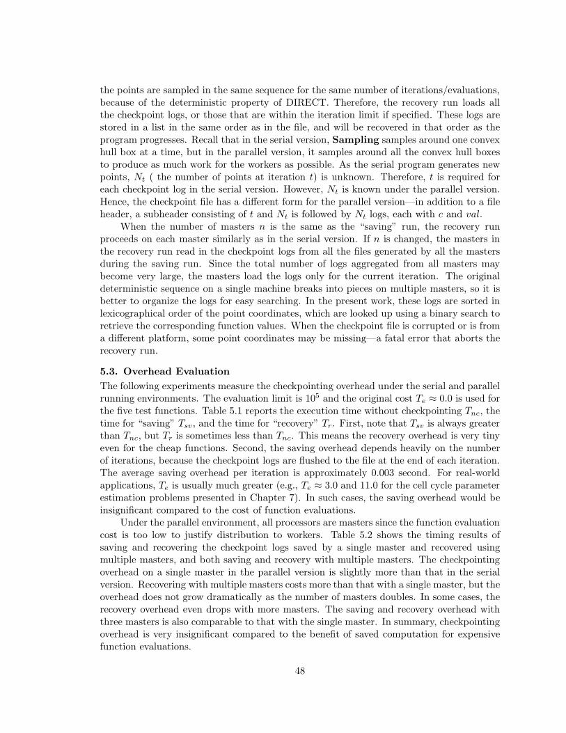
the points are sampled in the same sequence for the same number of iterations/evaluations,because of the deterministic property of DIRECT. Therefore, the recovery run loads allthe checkpoint logs, or those that are within the iteration limit if specified. These logs arestored in a list in the same order as in the file, and will be recovered in that order as theprogram progresses. Recall that in the serial version, Sampling samples around one convexhull box at a time, but in the parallel version, it samples around all the convex hull boxesto produce as much work for the workers as possible. As the serial program generates newpoints, Nt ( the number of points at iteration t) is unknown. Therefore, t is required foreach checkpoint log in the serial version. However, Nt is known under the parallel version.Hence, the checkpoint file has a different form for the parallel version—in addition to a fileheader, a subheader consisting of t and Nt is followed by Nt logs, each with c and val.
When the number of masters n is the same as the “saving” run, the recovery runproceeds on each master similarly as in the serial version. If n is changed, the masters inthe recovery run read in the checkpoint logs from all the files generated by all the mastersduring the saving run. Since the total number of logs aggregated from all masters maybecome very large, the masters load the logs only for the current iteration. The originaldeterministic sequence on a single machine breaks into pieces on multiple masters, so it isbetter to organize the logs for easy searching. In the present work, these logs are sorted inlexicographical order of the point coordinates, which are looked up using a binary search toretrieve the corresponding function values. When the checkpoint file is corrupted or is froma different platform, some point coordinates may be missing—a fatal error that aborts therecovery run.
5.3. Overhead Evaluation
The following experiments measure the checkpointing overhead under the serial and parallelrunning environments. The evaluation limit is 105 and the original cost Te ≈ 0.0 is used forthe five test functions. Table 5.1 reports the execution time without checkpointing Tnc, thetime for “saving” Tsv, and the time for “recovery” Tr. First, note that Tsv is always greaterthan Tnc, but Tr is sometimes less than Tnc. This means the recovery overhead is very tinyeven for the cheap functions. Second, the saving overhead depends heavily on the numberof iterations, because the checkpoint logs are flushed to the file at the end of each iteration.The average saving overhead per iteration is approximately 0.003 second. For real-worldapplications, Te is usually much greater (e.g., Te ≈ 3.0 and 11.0 for the cell cycle parameterestimation problems presented in Chapter 7). In such cases, the saving overhead would beinsignificant compared to the cost of function evaluations.
Under the parallel environment, all processors are masters since the function evaluationcost is too low to justify distribution to workers. Table 5.2 shows the timing results ofsaving and recovering the checkpoint logs saved by a single master and recovered usingmultiple masters, and both saving and recovery with multiple masters. The checkpointingoverhead on a single master in the parallel version is slightly more than that in the serialversion. Recovering with multiple masters costs more than that with a single master, but theoverhead does not grow dramatically as the number of masters doubles. In some cases, therecovery overhead even drops with more masters. The saving and recovery overhead withthree masters is also comparable to that with the single master. In summary, checkpointingoverhead is very insignificant compared to the benefit of saved computation for expensivefunction evaluations.
48
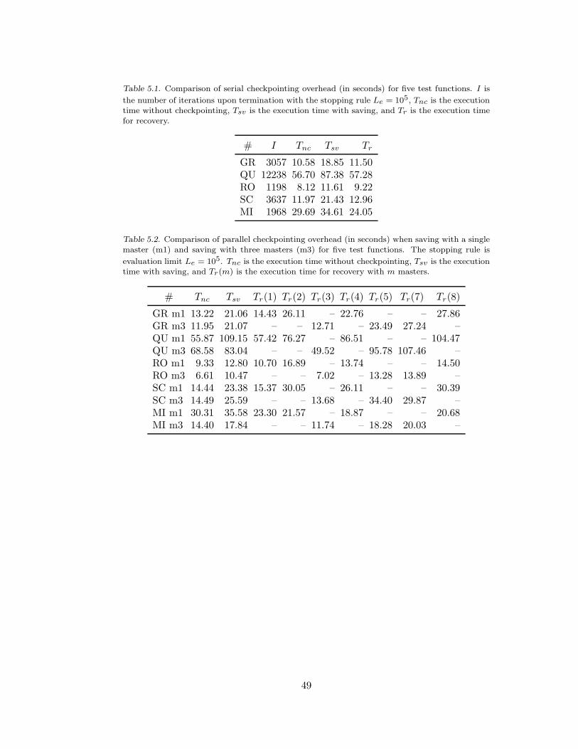
Table 5.1. Comparison of serial checkpointing overhead (in seconds) for five test functions. I is
the number of iterations upon termination with the stopping rule Le = 105, Tnc is the executiontime without checkpointing, Tsv is the execution time with saving, and Tr is the execution time
for recovery.
# I Tnc Tsv Tr
GR 3057 10.58 18.85 11.50QU 12238 56.70 87.38 57.28RO 1198 8.12 11.61 9.22SC 3637 11.97 21.43 12.96MI 1968 29.69 34.61 24.05
Table 5.2. Comparison of parallel checkpointing overhead (in seconds) when saving with a single
master (m1) and saving with three masters (m3) for five test functions. The stopping rule is
evaluation limit Le = 105. Tnc is the execution time without checkpointing, Tsv is the executiontime with saving, and Tr(m) is the execution time for recovery with m masters.
# Tnc Tsv Tr(1) Tr(2) Tr(3) Tr(4) Tr(5) Tr(7) Tr(8)
GR m1 13.22 21.06 14.43 26.11 – 22.76 – – 27.86GR m3 11.95 21.07 – – 12.71 – 23.49 27.24 –QU m1 55.87 109.15 57.42 76.27 – 86.51 – – 104.47QU m3 68.58 83.04 – – 49.52 – 95.78 107.46 –RO m1 9.33 12.80 10.70 16.89 – 13.74 – – 14.50RO m3 6.61 10.47 – – 7.02 – 13.28 13.89 –SC m1 14.44 23.38 15.37 30.05 – 26.11 – – 30.39SC m3 14.49 25.59 – – 13.68 – 34.40 29.87 –MI m1 30.31 35.58 23.30 21.57 – 18.87 – – 20.68MI m3 14.40 17.84 – – 11.74 – 18.28 20.03 –
49
CHAPTER 6: Performance Study, Modeling, and Analysis
Several optimization parameters and system characteristics listed in Table 6.1 are se-
lected for the performance sensitivity study. In fact, more input parameters are required to
define the optimization problem. For example, the upper and lower bounds of the design
domain define the search region. Varying the bounds certainly affects the convergence rate
as well as the total computational cost to reach the solution, so the proper bounding for
a particular problem deserves a thorough application-oriented study by researchers in that
field. In this section, upper and lower bounds are fixed for each problem as in Appendix A.
Table 6.1. Parameters and characteristics under study.
# Descriptionǫ Search tuning parameterNd Problem dimensionImax maximum iterationsNb number of evaluations per taskm number of subdomainsn number of masters per subdomaink number of workersTf objective function cost, secondsTcp point-to-point round trip cost, microsecondsTca one-to-all broadcast cost, microseconds
The first three parameters affect problem configuration. The parameter ǫ tunes the
search broadness as discussed in Chapter 2. The parameters Nd and Imax directly affect
the problem scale. Imax is also required to enable the local memory reduction technique
discussed in Chapter 3. Section 6.1 studies the parameters for problem configuration. The
parallel scheme parameters Nb, m, n, and k have great impact on both minimization perfor-
mance and parallel performance such as load balancing. In Section 6.2, these performance
metrics are analyzed theoretically and experimentally. The next subset {Tf , Tcp, Tca}
determines the task granularity defined as the ratio of the computation time to communi-
cation time per task. These parameters are addressed in Section 6.3, followed by detailed
discussions of the influence of these parameters on overhead and scalability in Section 6.4.
50
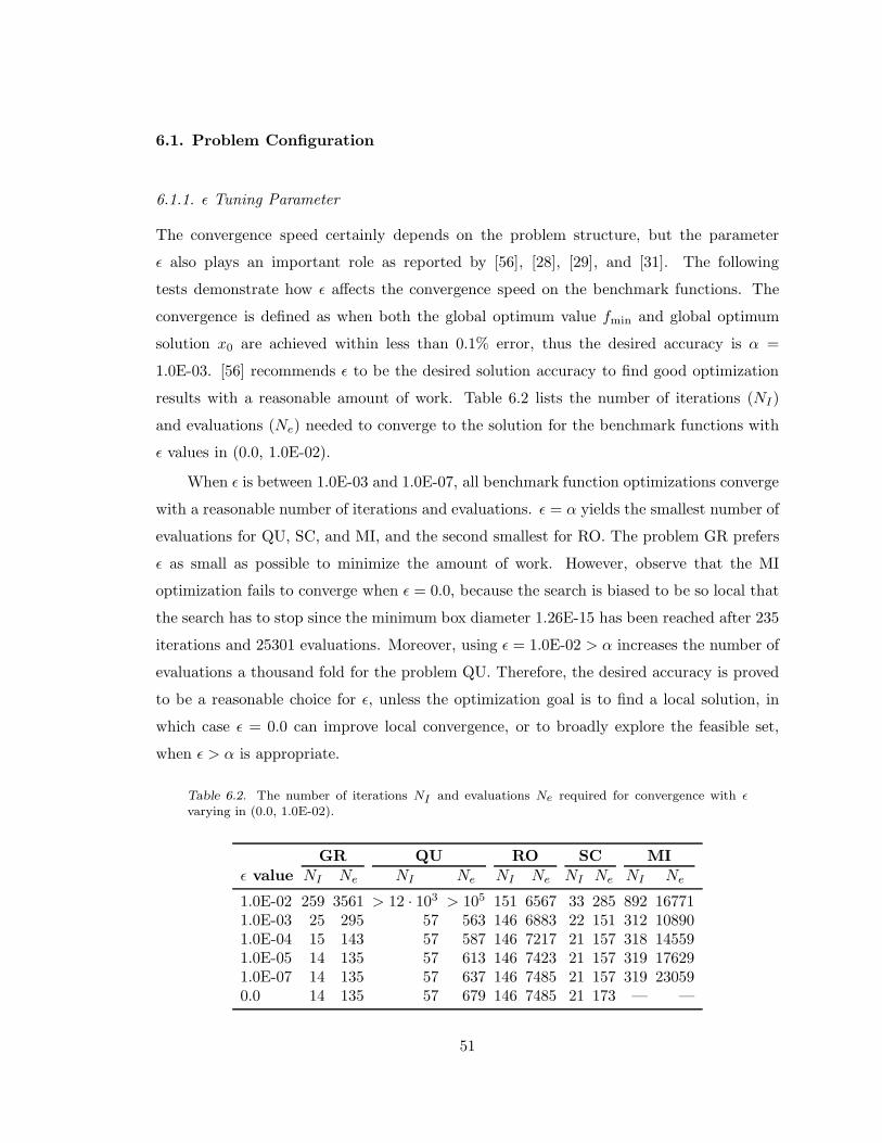
6.1. Problem Configuration
6.1.1. ǫ Tuning Parameter
The convergence speed certainly depends on the problem structure, but the parameter
ǫ also plays an important role as reported by [56], [28], [29], and [31]. The following
tests demonstrate how ǫ affects the convergence speed on the benchmark functions. The
convergence is defined as when both the global optimum value fmin and global optimum
solution x0 are achieved within less than 0.1% error, thus the desired accuracy is α =
1.0E-03. [56] recommends ǫ to be the desired solution accuracy to find good optimization
results with a reasonable amount of work. Table 6.2 lists the number of iterations (NI)
and evaluations (Ne) needed to converge to the solution for the benchmark functions with
ǫ values in (0.0, 1.0E-02).
When ǫ is between 1.0E-03 and 1.0E-07, all benchmark function optimizations converge
with a reasonable number of iterations and evaluations. ǫ = α yields the smallest number of
evaluations for QU, SC, and MI, and the second smallest for RO. The problem GR prefers
ǫ as small as possible to minimize the amount of work. However, observe that the MI
optimization fails to converge when ǫ = 0.0, because the search is biased to be so local that
the search has to stop since the minimum box diameter 1.26E-15 has been reached after 235
iterations and 25301 evaluations. Moreover, using ǫ = 1.0E-02 > α increases the number of
evaluations a thousand fold for the problem QU. Therefore, the desired accuracy is proved
to be a reasonable choice for ǫ, unless the optimization goal is to find a local solution, in
which case ǫ = 0.0 can improve local convergence, or to broadly explore the feasible set,
when ǫ > α is appropriate.
Table 6.2. The number of iterations NI and evaluations Ne required for convergence with ǫ
varying in (0.0, 1.0E-02).
GR QU RO SC MI
ǫ value NI Ne NI Ne NI Ne NI Ne NI Ne
1.0E-02 259 3561 > 12 · 103 > 105 151 6567 33 285 892 167711.0E-03 25 295 57 563 146 6883 22 151 312 108901.0E-04 15 143 57 587 146 7217 21 157 318 145591.0E-05 14 135 57 613 146 7423 21 157 319 176291.0E-07 14 135 57 637 146 7485 21 157 319 230590.0 14 135 57 679 146 7485 21 173 — —
51
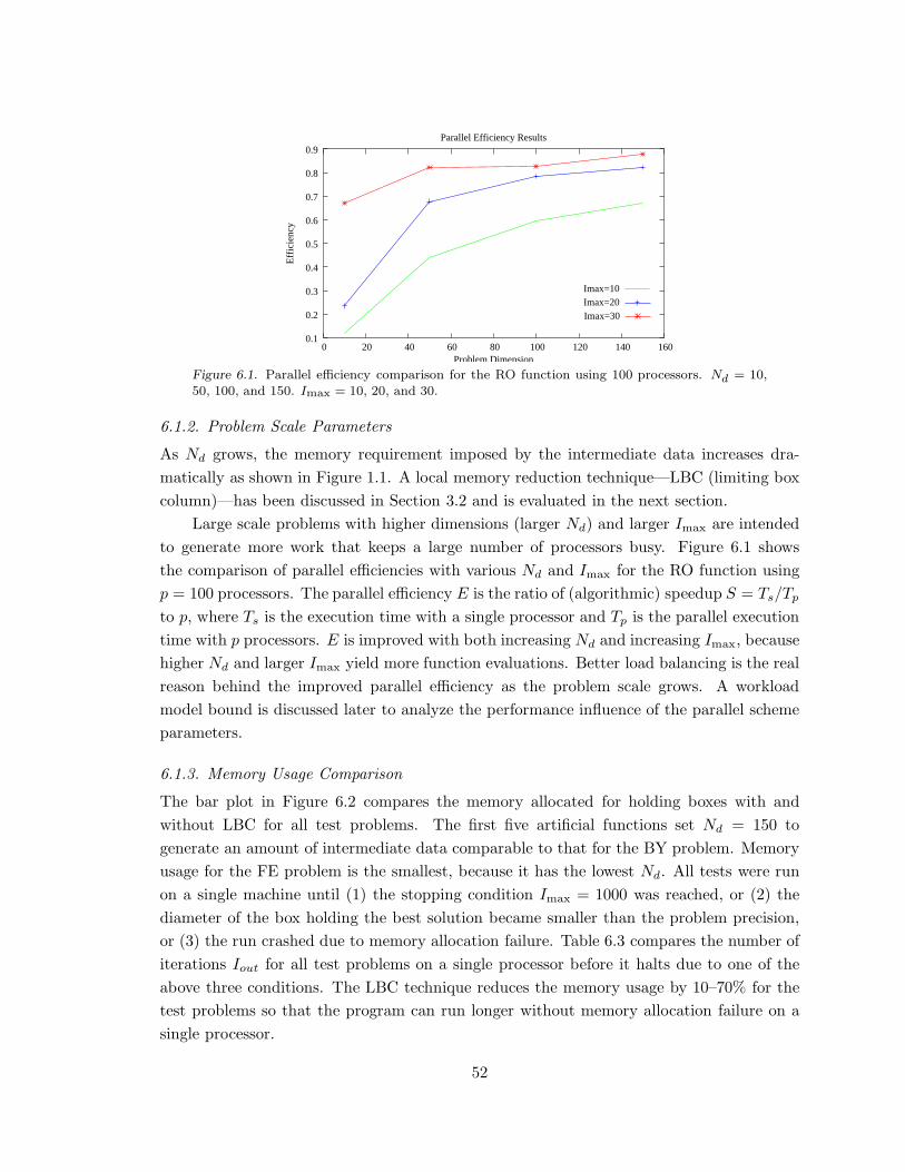
0.1
0.2
0.3
0.4
0.5
0.6
0.7
0.8
0.9
0 20 40 60 80 100 120 140 160
Effi
cien
cy
Problem Dimension
Parallel Efficiency Results
Imax=10Imax=20Imax=30
Figure 6.1. Parallel efficiency comparison for the RO function using 100 processors. Nd = 10,
50, 100, and 150. Imax = 10, 20, and 30.
6.1.2. Problem Scale Parameters
As Nd grows, the memory requirement imposed by the intermediate data increases dra-
matically as shown in Figure 1.1. A local memory reduction technique—LBC (limiting box
column)—has been discussed in Section 3.2 and is evaluated in the next section.
Large scale problems with higher dimensions (larger Nd) and larger Imax are intended
to generate more work that keeps a large number of processors busy. Figure 6.1 shows
the comparison of parallel efficiencies with various Nd and Imax for the RO function using
p = 100 processors. The parallel efficiency E is the ratio of (algorithmic) speedup S = Ts/Tp
to p, where Ts is the execution time with a single processor and Tp is the parallel execution
time with p processors. E is improved with both increasing Nd and increasing Imax, because
higher Nd and larger Imax yield more function evaluations. Better load balancing is the real
reason behind the improved parallel efficiency as the problem scale grows. A workload
model bound is discussed later to analyze the performance influence of the parallel scheme
parameters.
6.1.3. Memory Usage Comparison
The bar plot in Figure 6.2 compares the memory allocated for holding boxes with and
without LBC for all test problems. The first five artificial functions set Nd = 150 to
generate an amount of intermediate data comparable to that for the BY problem. Memory
usage for the FE problem is the smallest, because it has the lowest Nd. All tests were run
on a single machine until (1) the stopping condition Imax = 1000 was reached, or (2) the
diameter of the box holding the best solution became smaller than the problem precision,
or (3) the run crashed due to memory allocation failure. Table 6.3 compares the number of
iterations Iout for all test problems on a single processor before it halts due to one of the
above three conditions. The LBC technique reduces the memory usage by 10–70% for the
test problems so that the program can run longer without memory allocation failure on a
single processor.
52
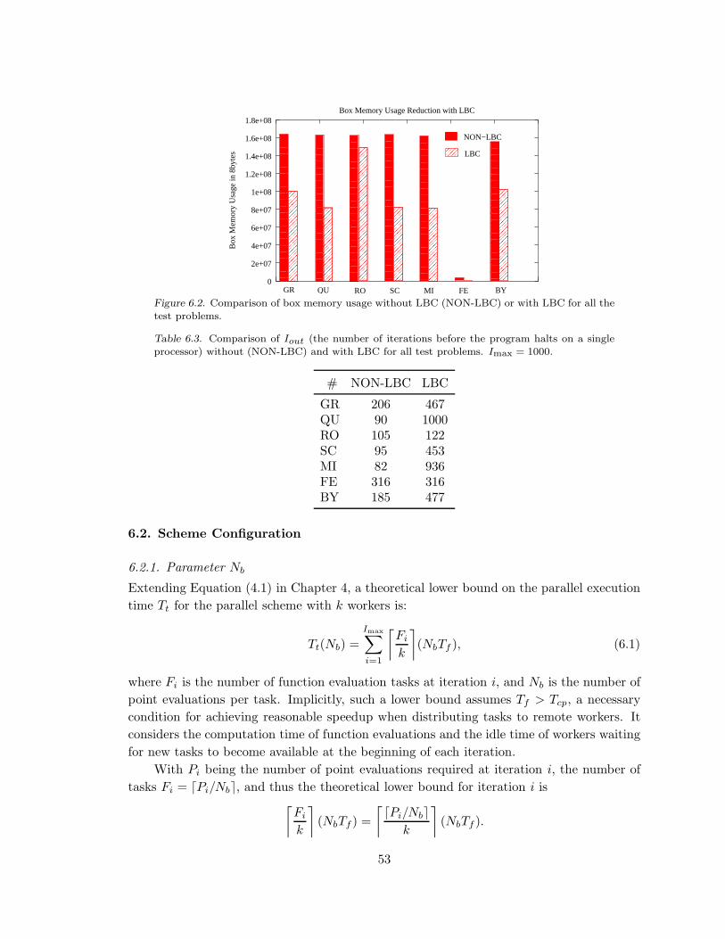
�������
�������
������������
������������
�������
�������
�������
�������
����������������
����������������
��������
��������
����
������������������������������������������������
������������������������������������������������
������������������������������������������������
������������������������������������������������
������������������������
������������������������
������������������������
������������������������
������������������������
������������������������
�����������������������
�����������������������
��������
NON−LBC
LBC
GR QU RO SC MI FE BY 0
2e+07
4e+07
6e+07
8e+07
1e+08
1.2e+08
1.4e+08
1.6e+08
1.8e+08
Box
Mem
ory
Usa
ge in
8by
tes
Box Memory Usage Reduction with LBC
Figure 6.2. Comparison of box memory usage without LBC (NON-LBC) or with LBC for all the
test problems.
Table 6.3. Comparison of Iout (the number of iterations before the program halts on a single
processor) without (NON-LBC) and with LBC for all test problems. Imax = 1000.
# NON-LBC LBC
GR 206 467QU 90 1000RO 105 122SC 95 453MI 82 936FE 316 316BY 185 477
6.2. Scheme Configuration
6.2.1. Parameter Nb
Extending Equation (4.1) in Chapter 4, a theoretical lower bound on the parallel execution
time Tt for the parallel scheme with k workers is:
Tt(Nb) =
Imax∑
i=1
⌈
Fi
k
⌉
(NbTf ), (6.1)
where Fi is the number of function evaluation tasks at iteration i, and Nb is the number of
point evaluations per task. Implicitly, such a lower bound assumes Tf > Tcp, a necessary
condition for achieving reasonable speedup when distributing tasks to remote workers. It
considers the computation time of function evaluations and the idle time of workers waiting
for new tasks to become available at the beginning of each iteration.
With Pi being the number of point evaluations required at iteration i, the number of
tasks Fi = ⌈Pi/Nb⌉, and thus the theoretical lower bound for iteration i is⌈
Fi
k
⌉
(NbTf ) =
⌈⌈Pi/Nb⌉k
⌉
(NbTf ).
53
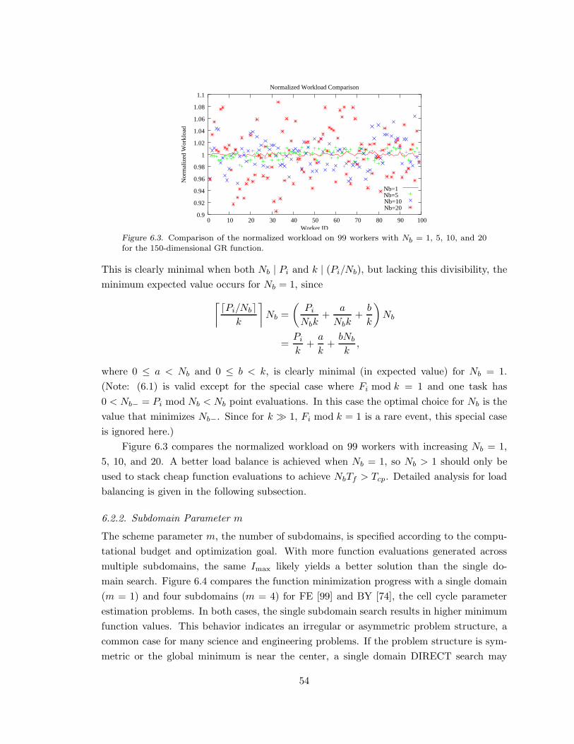
Nb=20Nb=10Nb=5Nb=1
0.9
0.92
0.94
0.96
0.98
1
1.02
1.04
1.06
1.08
1.1
0 10 20 30 40 50 60 70 80 90 100
Nor
mal
ized
Wor
kloa
d
Worker ID
Normalized Workload Comparison
Figure 6.3. Comparison of the normalized workload on 99 workers with Nb = 1, 5, 10, and 20
for the 150-dimensional GR function.
This is clearly minimal when both Nb | Pi and k | (Pi/Nb), but lacking this divisibility, the
minimum expected value occurs for Nb = 1, since
⌈⌈Pi/Nb⌉k
⌉
Nb =
(
Pi
Nbk+
a
Nbk+
b
k
)
Nb
=Pi
k+
a
k+
bNb
k,
where 0 ≤ a < Nb and 0 ≤ b < k, is clearly minimal (in expected value) for Nb = 1.
(Note: (6.1) is valid except for the special case where Fi mod k = 1 and one task has
0 < Nb− = Pi mod Nb < Nb point evaluations. In this case the optimal choice for Nb is the
value that minimizes Nb−. Since for k ≫ 1, Fi mod k = 1 is a rare event, this special case
is ignored here.)
Figure 6.3 compares the normalized workload on 99 workers with increasing Nb = 1,
5, 10, and 20. A better load balance is achieved when Nb = 1, so Nb > 1 should only be
used to stack cheap function evaluations to achieve NbTf > Tcp. Detailed analysis for load
balancing is given in the following subsection.
6.2.2. Subdomain Parameter m
The scheme parameter m, the number of subdomains, is specified according to the compu-
tational budget and optimization goal. With more function evaluations generated across
multiple subdomains, the same Imax likely yields a better solution than the single do-
main search. Figure 6.4 compares the function minimization progress with a single domain
(m = 1) and four subdomains (m = 4) for FE [99] and BY [74], the cell cycle parameter
estimation problems. In both cases, the single subdomain search results in higher minimum
function values. This behavior indicates an irregular or asymmetric problem structure, a
common case for many science and engineering problems. If the problem structure is sym-
metric or the global minimum is near the center, a single domain DIRECT search may
54
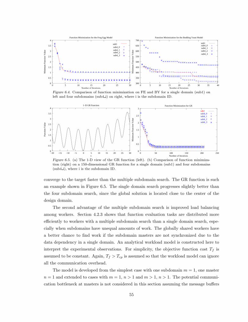
0
0.5
1
1.5
2
2.5
3
3.5
4
0 5 10 15 20 25 30
Min
imum
Fun
ctio
n V
alue
Number of Iterations
Function Minimization for the Frog Egg Model
sub1sub4_0
sub4_2sub4_1
sub4_3
300
350
400
450
500
550
600
650
700
0 5 10 15 20 25 30 35 40
Min
imum
Fun
ctio
n V
alue
Number of Iterations
Function Minimization for the Budding Yeast Model
sub4_3sub4_2sub4_1sub4_0sub1
Figure 6.4. Comparison of function minimization on FE and BY for a single domain (sub1) on
left and four subdomains (sub4 i) on right, where i is the subdomain ID.
0
0.5
1
1.5
2
2.5
3
3.5
4
−20 −15 −10 −5 0 5 10 15 20 25 30
Fun
ctio
n V
alue
x
1−D GR Function
0
0.5
1
1.5
2
2.5
3
0 50 100 150 200 250
Min
imum
Fun
ctio
n V
alue
Number of Iterations
Function Minimization for GR
sub4_3sub4_2sub4_1sub4_0sub1
Figure 6.5. (a) The 1-D view of the GR function (left). (b) Comparison of function minimiza-
tion (right) on a 150-dimensional GR function for a single domain (sub1) and four subdomains
(sub4 i), where i is the subdomain ID.
converge to the target faster than the multiple subdomain search. The GR function is such
an example shown in Figure 6.5. The single domain search progresses slightly better than
the four subdomain search, since the global solution is located close to the center of the
design domain.
The second advantage of the multiple subdomain search is improved load balancing
among workers. Section 4.2.3 shows that function evaluation tasks are distributed more
efficiently to workers with a multiple subdomain search than a single domain search, espe-
cially when subdomains have unequal amounts of work. The globally shared workers have
a better chance to find work if the subdomain masters are not synchronized due to the
data dependency in a single domain. An analytical workload model is constructed here to
interpret the experimental observations. For simplicity, the objective function cost Tf is
assumed to be constant. Again, Tf > Tcp is assumed so that the workload model can ignore
all the communication overhead.
The model is developed from the simplest case with one subdomain m = 1, one master
n = 1 and extended to cases with m = 1, n > 1 and m > 1, n > 1. The potential communi-
cation bottleneck at masters is not considered in this section assuming the message buffers
55
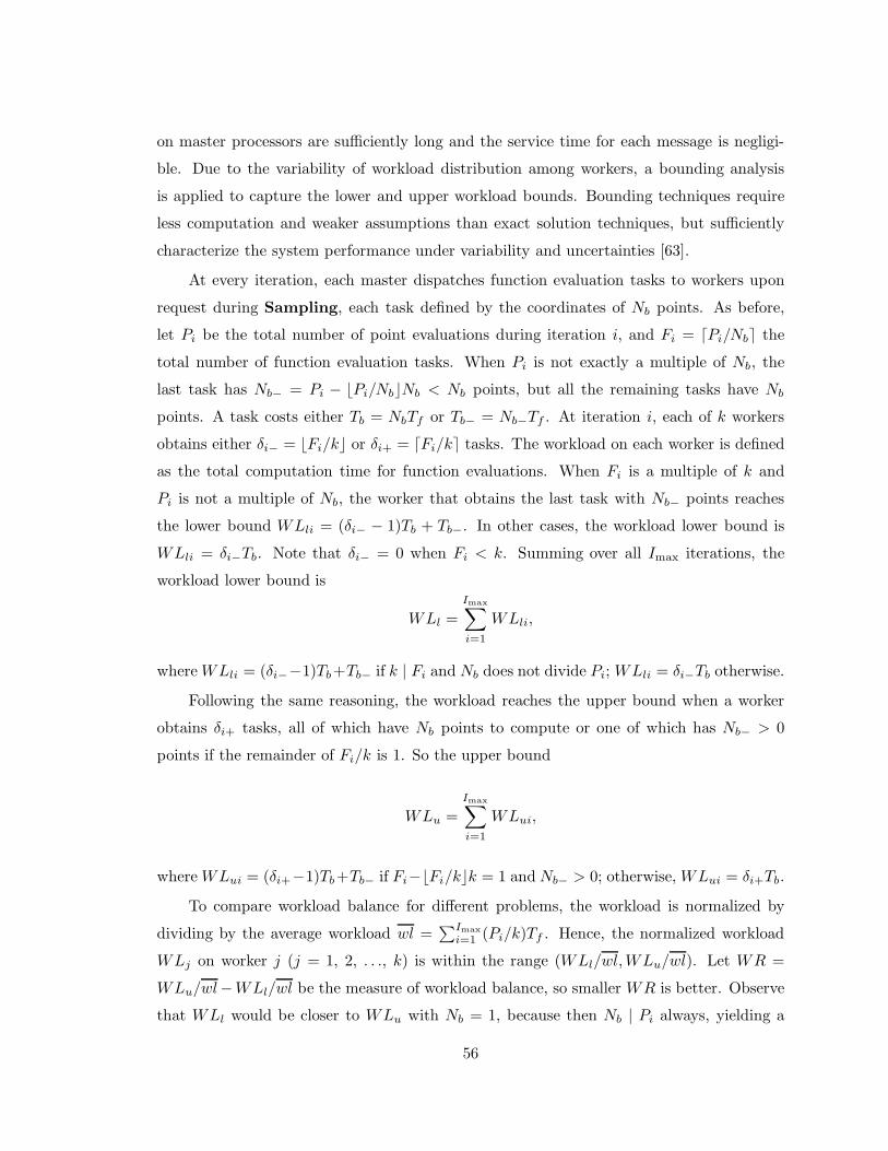
on master processors are sufficiently long and the service time for each message is negligi-
ble. Due to the variability of workload distribution among workers, a bounding analysis
is applied to capture the lower and upper workload bounds. Bounding techniques require
less computation and weaker assumptions than exact solution techniques, but sufficiently
characterize the system performance under variability and uncertainties [63].
At every iteration, each master dispatches function evaluation tasks to workers upon
request during Sampling, each task defined by the coordinates of Nb points. As before,
let Pi be the total number of point evaluations during iteration i, and Fi = ⌈Pi/Nb⌉ the
total number of function evaluation tasks. When Pi is not exactly a multiple of Nb, the
last task has Nb− = Pi − ⌊Pi/Nb⌋Nb < Nb points, but all the remaining tasks have Nb
points. A task costs either Tb = NbTf or Tb− = Nb−Tf . At iteration i, each of k workers
obtains either δi− = ⌊Fi/k⌋ or δi+ = ⌈Fi/k⌉ tasks. The workload on each worker is defined
as the total computation time for function evaluations. When Fi is a multiple of k and
Pi is not a multiple of Nb, the worker that obtains the last task with Nb− points reaches
the lower bound WLli = (δi− − 1)Tb + Tb−. In other cases, the workload lower bound is
WLli = δi−Tb. Note that δi− = 0 when Fi < k. Summing over all Imax iterations, the
workload lower bound is
WLl =
Imax∑
i=1
WLli,
where WLli = (δi−−1)Tb+Tb− if k | Fi and Nb does not divide Pi; WLli = δi−Tb otherwise.
Following the same reasoning, the workload reaches the upper bound when a worker
obtains δi+ tasks, all of which have Nb points to compute or one of which has Nb− > 0
points if the remainder of Fi/k is 1. So the upper bound
WLu =
Imax∑
i=1
WLui,
where WLui = (δi+−1)Tb+Tb− if Fi−⌊Fi/k⌋k = 1 and Nb− > 0; otherwise, WLui = δi+Tb.
To compare workload balance for different problems, the workload is normalized by
dividing by the average workload wl =∑Imax
i=1 (Pi/k)Tf . Hence, the normalized workload
WLj on worker j (j = 1, 2, . . ., k) is within the range (WLl/wl,WLu/wl). Let WR =
WLu/wl−WLl/wl be the measure of workload balance, so smaller WR is better. Observe
that WLl would be closer to WLu with Nb = 1, because then Nb | Pi always, yielding a
56

Model WLModel WL
Exp WL
Nb
l
u
lExp WLu
0.2
0.4
0.6
0.8
1
1.2
1.4
1.6
0 2 4 6 8 10 12 14 16 18 20
Nor
mal
ized
Wor
kloa
d
Comparison of Experimental and Model Workload Bounds
Figure 6.6. Comparison of the normalized workload bounds based on the model and the experi-
ments with 99 workers and Nb = 1, 5, 10, and 20 for the 150-dimensional GR function.
���
���
(c)(b)(a)GR QU RO MI SC BY GR QU RO MI SC BY GR QU RO MI SC BY
Nor
mal
ized
Wor
kloa
d
Workload Range Comparison
0.96
0.92
0.9
0.94
0.98
1.08
1.06
1.04
1.02
1
1.1
1
0.975
0.98
0.985
0.99
0.995
1.01
1.005
1
1.015
1.02
1.025
0.98
0.985
0.99
0.995
1.005
1.01
1.015
1.02
Figure 6.7. Comparison of the workload ranges based on the model (grey) and the experiments
(black) for (a) a single domain search with 1 master and 99 workers, (b) a single domain search
with 4 masters and 196 workers, and (c) a four subdomain search with 1 master per subdomain
and totally 196 workers. Nb = 1. The vertical bars, left to right, correspond respectively to
problems GR, QU, RO, SC, MI, BY. Imax = 90 and Nd = 150 for the artificial problems.
Imax = 40 and Nd = 143 for the BY problem.
larger WLl. Recall that Nb = 1 also gives the smallest possible WLu =∑Imax
i=1 ⌈Pi/k⌉Tf ≤∑Imax
i=1 ⌈⌈Pi/Nb⌉/k⌉NbTf .
Figure 6.6 plots the workload ranges estimated with the model and the actual workload
ranges measured from experiments for different Nb values. All the experimental workload
bounds are within the model estimation, but the difference between the experimental bounds
and the model estimation becomes larger as Nb increases. The model sums up the lowest
workload among workers over all iterations, while in reality, the workload on a particular
worker has a fair chance to be the lowest at every iteration. Therefore, the load balancing
measurement is better than the model estimation because of the inherent randomness of
the parallel scheme.
For high dimensional test problems, Figure 6.7(a) compares the workload ranges based
on the model and the experiments for a single domain search using one master and 99
57
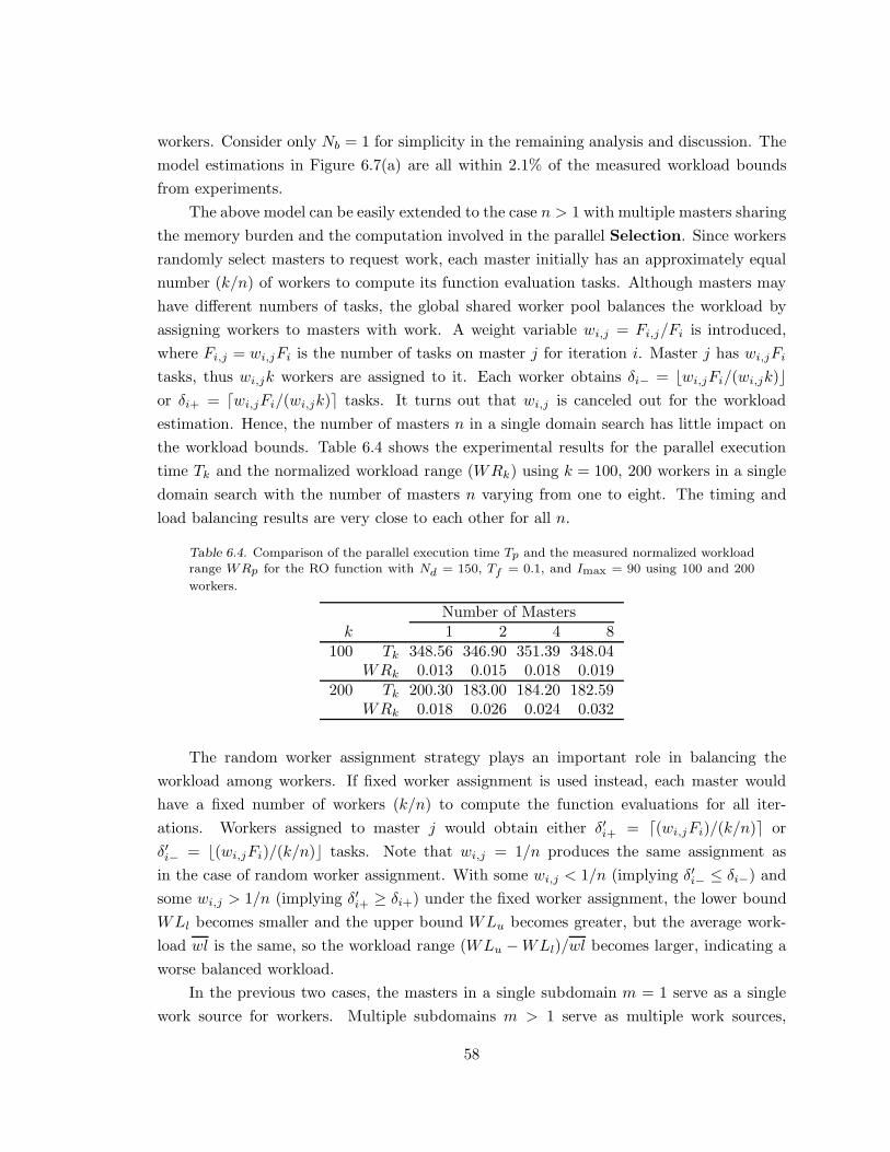
workers. Consider only Nb = 1 for simplicity in the remaining analysis and discussion. The
model estimations in Figure 6.7(a) are all within 2.1% of the measured workload bounds
from experiments.
The above model can be easily extended to the case n > 1 with multiple masters sharing
the memory burden and the computation involved in the parallel Selection. Since workers
randomly select masters to request work, each master initially has an approximately equal
number (k/n) of workers to compute its function evaluation tasks. Although masters may
have different numbers of tasks, the global shared worker pool balances the workload by
assigning workers to masters with work. A weight variable wi,j = Fi,j/Fi is introduced,
where Fi,j = wi,jFi is the number of tasks on master j for iteration i. Master j has wi,jFi
tasks, thus wi,jk workers are assigned to it. Each worker obtains δi− = ⌊wi,jFi/(wi,jk)⌋or δi+ = ⌈wi,jFi/(wi,jk)⌉ tasks. It turns out that wi,j is canceled out for the workload
estimation. Hence, the number of masters n in a single domain search has little impact on
the workload bounds. Table 6.4 shows the experimental results for the parallel execution
time Tk and the normalized workload range (WRk) using k = 100, 200 workers in a single
domain search with the number of masters n varying from one to eight. The timing and
load balancing results are very close to each other for all n.
Table 6.4. Comparison of the parallel execution time Tp and the measured normalized workload
range WRp for the RO function with Nd = 150, Tf = 0.1, and Imax = 90 using 100 and 200
workers.
Number of Mastersk 1 2 4 8
100 Tk 348.56 346.90 351.39 348.04WRk 0.013 0.015 0.018 0.019
200 Tk 200.30 183.00 184.20 182.59WRk 0.018 0.026 0.024 0.032
The random worker assignment strategy plays an important role in balancing the
workload among workers. If fixed worker assignment is used instead, each master would
have a fixed number of workers (k/n) to compute the function evaluations for all iter-
ations. Workers assigned to master j would obtain either δ′i+ = ⌈(wi,jFi)/(k/n)⌉ or
δ′i− = ⌊(wi,jFi)/(k/n)⌋ tasks. Note that wi,j = 1/n produces the same assignment as
in the case of random worker assignment. With some wi,j < 1/n (implying δ′i− ≤ δi−) and
some wi,j > 1/n (implying δ′i+ ≥ δi+) under the fixed worker assignment, the lower bound
WLl becomes smaller and the upper bound WLu becomes greater, but the average work-
load wl is the same, so the workload range (WLu − WLl)/wl becomes larger, indicating a
worse balanced workload.
In the previous two cases, the masters in a single subdomain m = 1 serve as a single
work source for workers. Multiple subdomains m > 1 serve as multiple work sources,
58

because the masters from different subdomains are not synchronized to update intermediate
results or to compute the global convex hull boxes. A similar weight variable w′j is used in
this case to estimate the number of workers assigned for the subdomain j:
w′j =
Imax∑
i=1
Fi,j
/
m∑
j=1
Imax∑
i=1
Fi,j , (6.2)
where Fi,j denotes the number of tasks at iteration i for subdomain j. w′j is based on the
overall tasks from all iterations because subdomains are asynchronous. In contrast, wi,j in
the single domain case is defined for each iteration due to the global synchronization inside
a subdomain. For subdomain j, the average workload is wlj =∑Imax
i=1 Fi,j/(w′jk)Tb. The
workload lower bound in subdomain j is WLlj =∑Imax
i=1 ⌊Fi,j/(w′jk)⌋Tb, where Tb = Tf
because Nb = 1; the workload upper bound is WLuj =∑Imax
i=1 ⌈Fi,j/(w′jk)⌉Tb. Hence, the
overall normalized workload range is
(
min1≤j≤m
(WLlj/wlj), max1≤j≤m
(WLuj/wlj)
)
across all m subdomains. Figure 6.7(c) compares the model estimated workload ranges
with the experimental results for a four subdomain search using 196 workers and four
masters, one per subdomain. All the experimental workload results fall within the 1.5%
ranges estimated by the model. Due to the randomness of workers’ requests to masters,
the experimental workload is better balanced than the (worst case) model estimation. For
comparison, the workload ranges based on the model and experiments for a single domain
search using the same number of masters and workers are shown in Figure 6.7(b). To keep
the problem the same as in the four subdomain search, the single domain search is applied
to each of the four subdomains sequentially using 49 workers and one master. The workload
is normalized over the total workload of the four runs. The model estimated range for the
single domain is wider than that for the four subdomains. This estimation is verified by
the experimental results, which present smaller ranges for the four subdomain search (dark
bars in Figure 6.7(c)) than for the single domain search (dark bars in Figure 6.7(b)).
6.2.3. Parameter n
The number n of masters affects the efficiency of Selection and data distribution. Convex
hull computation is the key component in Selection. The parallel Selection involves both
local and global computation of convex hull boxes. First, each subdomain master computes
the local convex hull boxes. Next, the root subdomain master gathers all the local convex
59

0
50
100
150
200
250
0 5 10 15 20 25 30 35
Sec
onds
Number of Masters
GR
QU
ROSC
MI
Average Selection Cost per Master
Figure 6.8. The average Selection cost per master increases as n grows from 1 to 32 for test
problems. Imax = Iout with LBC support listed in Table 3.3 in Section 3.3.5.
4e+07
6e+07
8e+07
1e+08
1.2e+08
1.4e+08
1.6e+08
0 5 10 15 20 25 30 35
8 B
ytes
Number of Masters
Average Box Memory Usage per Master
MI
SC
RO
QU
GR
Figure 6.9. The average box memory size decreases as n grows from 1 to 32 for test problems.
Imax = Iout with LBC support listed in Table 4.2.
hulls to find a global convex hull set of boxes. Finally, each subdomain master starts
Sampling on its own portion of the convex hull boxes.
Recall that for the local convex hull computation, the gift-wrapping algorithm with
complexity O(N2) [64] is preferred because it requires no extra space. A faster algorithm,
Graham’s scan [34], is used for the global convex hull computation at the root subdomain
master. It takes O(N) operations because the gathered local convex hull boxes are already
sorted, saving O(N log(N)) operations required for sorting at the root subdomain master.
Although the Graham’s scan needs a stack for back-tracking, the buffer for merging local
convex hull boxes also serves as a stack of boxes, which are indexed by integer pointers
for back-tracking. As n increases, the number of sets of local convex hull boxes grows, and
more boxes are merged at the root subdomain master for the final global computation. Since
the root needs to gather from all and broadcast to all at each iteration, the communication
overhead may overshadow the benefit of sharing the memory burden. Therefore, the value of
n should be large enough to accommodate the intermediate data, yet no larger to minimize
the network traffic for global communication.
60
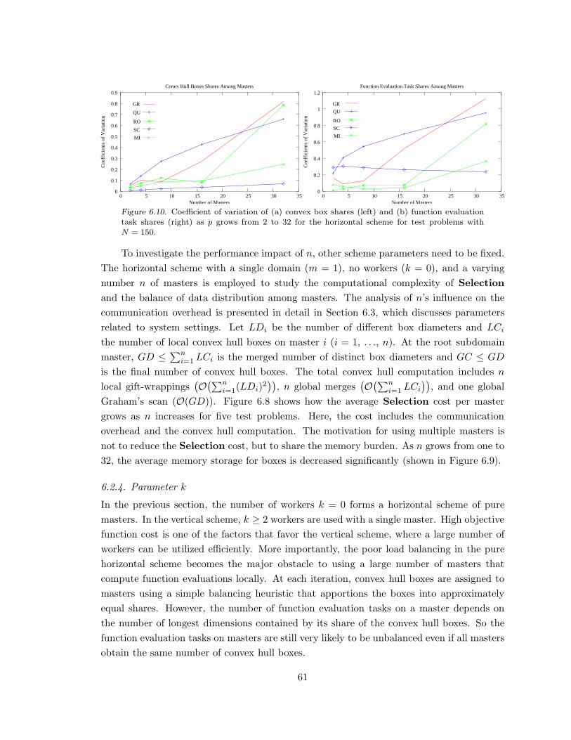
0
0.1
0.2
0.3
0.4
0.5
0.6
0.7
0.8
0.9
0 5 10 15 20 25 30 35Number of Masters
Conex Hull Boxes Shares Among Masters
GR
QU
RO
SC
MI
Coe
ffici
ents
of V
aria
tion
0
0.2
0.4
0.6
0.8
1
1.2
0 5 10 15 20 25 30 35Number of Masters
Function Evaluation Task Shares Among Masters
QU
RO
SC
MI
GR
Coe
ffici
ents
of V
aria
tion
Figure 6.10. Coefficient of variation of (a) convex box shares (left) and (b) function evaluation
task shares (right) as p grows from 2 to 32 for the horizontal scheme for test problems with
N = 150.
To investigate the performance impact of n, other scheme parameters need to be fixed.
The horizontal scheme with a single domain (m = 1), no workers (k = 0), and a varying
number n of masters is employed to study the computational complexity of Selection
and the balance of data distribution among masters. The analysis of n’s influence on the
communication overhead is presented in detail in Section 6.3, which discusses parameters
related to system settings. Let LDi be the number of different box diameters and LCi
the number of local convex hull boxes on master i (i = 1, . . ., n). At the root subdomain
master, GD ≤ ∑n
i=1 LCi is the merged number of distinct box diameters and GC ≤ GD
is the final number of convex hull boxes. The total convex hull computation includes n
local gift-wrappings(
O(∑n
i=1(LDi)2))
, n global merges(
O(∑n
i=1 LCi
))
, and one global
Graham’s scan (O(GD)). Figure 6.8 shows how the average Selection cost per master
grows as n increases for five test problems. Here, the cost includes the communication
overhead and the convex hull computation. The motivation for using multiple masters is
not to reduce the Selection cost, but to share the memory burden. As n grows from one to
32, the average memory storage for boxes is decreased significantly (shown in Figure 6.9).
6.2.4. Parameter k
In the previous section, the number of workers k = 0 forms a horizontal scheme of pure
masters. In the vertical scheme, k ≥ 2 workers are used with a single master. High objective
function cost is one of the factors that favor the vertical scheme, where a large number of
workers can be utilized efficiently. More importantly, the poor load balancing in the pure
horizontal scheme becomes the major obstacle to using a large number of masters that
compute function evaluations locally. At each iteration, convex hull boxes are assigned to
masters using a simple balancing heuristic that apportions the boxes into approximately
equal shares. However, the number of function evaluation tasks on a master depends on
the number of longest dimensions contained by its share of the convex hull boxes. So the
function evaluation tasks on masters are still very likely to be unbalanced even if all masters
obtain the same number of convex hull boxes.
61

Finding an optimal convex hull box assignment that minimizes the variance of the com-
bined number of longest dimensions on all masters is an NP-complete problem similar to the
knapsack or bin packing problems [64]. Although a polynomial time approximate solution
is available (i.e., dynamic programming), it does not solve all the balancing problems. Even
if a supposedly optimal box assignment is found, a load imbalance still occurs when (1) an
insufficient number of convex hull boxes is generated, or (2) Tf varies at different sample
points. The first cause is inevitable in early stages of the DIRECT search, and it also
happens more often for low dimension problems or problems with certain structures that
produce a small number of convex hull boxes. The second cause is also common in many
engineering design problems, such as the ray-tracing technique and WCDMA simulation in
wireless communication system design [42] [47] [48].
Figure 6.10 shows the coefficient of variation (a) cb for the convex hull box shares per
processor and (b) cf for the function evaluation task shares per processor with p = 2, 4, 8,
16, 32 for test problems with N = 150 and Imax = Iout, the maximum number of iterations
before the program halts on a single processor with the LBC support (see Table 6.3).
The general trend is that both the convex hull and the function evaluation shares become
less balanced as p grows except for the problem SC. For cb shown in Figure 6.10(a), the
problems GR, QU, and RO have a sharp increase, but the problems SC and MI increase
slightly, because a larger number of convex hull boxes are generated per iteration for the last
two problems (see Table 6.5, a list of the average convex hull boxes Nbox =∑Iout
i=1 Ci/Iout
and function evaluation tasks per iteration Nf =∑Iout
i=1 Fi/Iout, where Ci is the number
of convex hull boxes and Fi is the number of function evaluation tasks at iteration i). As
the only exception, the problem SC has an improved function evaluation task balance even
though its convex hull box balance becomes worse as p grows. However, if more than the
necessary number of processors are used, i.e., p > Nbox, the problem SC will eventually
become unbalanced on convex hull box and function evaluation task distribution among
master processors.
Table 6.5. Comparison of the average number of convex hull boxes Nbox and function evaluation
tasks Nf per iteration for test problems.
# Nbox Nf
GR 13.341 2990.2QU 10.197 2007.8RO 16.025 4234.7SC 103.52 17152.0MI 26.521 5942.0
62
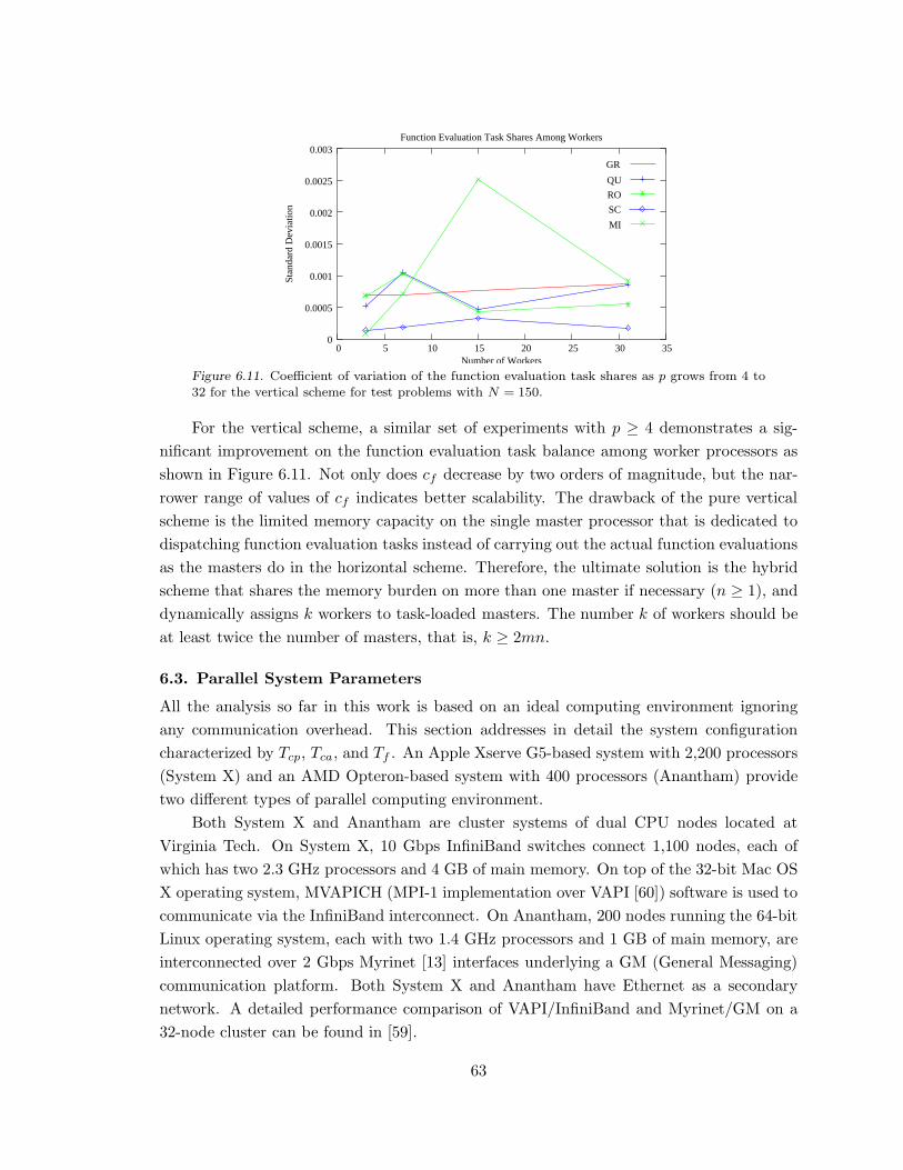
0
0.0005
0.001
0.0015
0.002
0.0025
0.003
0 5 10 15 20 25 30 35Number of Workers
Function Evaluation Task Shares Among Workers
Sta
ndar
d D
evia
tion
MI
SC
RO
QU
GR
Figure 6.11. Coefficient of variation of the function evaluation task shares as p grows from 4 to
32 for the vertical scheme for test problems with N = 150.
For the vertical scheme, a similar set of experiments with p ≥ 4 demonstrates a sig-
nificant improvement on the function evaluation task balance among worker processors as
shown in Figure 6.11. Not only does cf decrease by two orders of magnitude, but the nar-
rower range of values of cf indicates better scalability. The drawback of the pure vertical
scheme is the limited memory capacity on the single master processor that is dedicated to
dispatching function evaluation tasks instead of carrying out the actual function evaluations
as the masters do in the horizontal scheme. Therefore, the ultimate solution is the hybrid
scheme that shares the memory burden on more than one master if necessary (n ≥ 1), and
dynamically assigns k workers to task-loaded masters. The number k of workers should be
at least twice the number of masters, that is, k ≥ 2mn.
6.3. Parallel System Parameters
All the analysis so far in this work is based on an ideal computing environment ignoring
any communication overhead. This section addresses in detail the system configuration
characterized by Tcp, Tca, and Tf . An Apple Xserve G5-based system with 2,200 processors
(System X) and an AMD Opteron-based system with 400 processors (Anantham) provide
two different types of parallel computing environment.
Both System X and Anantham are cluster systems of dual CPU nodes located at
Virginia Tech. On System X, 10 Gbps InfiniBand switches connect 1,100 nodes, each of
which has two 2.3 GHz processors and 4 GB of main memory. On top of the 32-bit Mac OS
X operating system, MVAPICH (MPI-1 implementation over VAPI [60]) software is used to
communicate via the InfiniBand interconnect. On Anantham, 200 nodes running the 64-bit
Linux operating system, each with two 1.4 GHz processors and 1 GB of main memory, are
interconnected over 2 Gbps Myrinet [13] interfaces underlying a GM (General Messaging)
communication platform. Both System X and Anantham have Ethernet as a secondary
network. A detailed performance comparison of VAPI/InfiniBand and Myrinet/GM on a
32-node cluster can be found in [59].
63

h_p3v_p3h_p4v_p4h_p5v_p5
Tflog10
0.1
0.2
0.3
0.4
0.5
0.6
0.7
0.8
0.9
−5 −4.5 −4 −3.5 −3 −2.5 −2 −1.5 −1
Effi
cien
cy
Parallel Efficiency on System X
h_p3v_p3h_p4v_p4h_p5v_p5
log10
Tf
0.1
0.2
0.3
0.4
0.5
0.6
0.7
0.8
0.9
−5 −4.5 −4 −3.5 −3 −2.5 −2 −1.5 −1
Effi
cien
cy
Parallel Efficiency on Anantham
Figure 6.12. Comparison of parallel efficiency as Tf changes in the range (0, 0.1) using p = 3, 4,
and 5 processors for the 150-dimensional GR function with Imax = 90 on System X (left) and
Anantham (right). “v ” stands for the vertical scheme and “h ” for the horizontal scheme.
log10Tflog
10Tf
p3p4p5
Vertical Scheme Horizontal Scheme
−0.04
−0.02
0
0.02
0.04
0.06
0.08
0.1
−5 −4 −3 −2 −1 −5 −4 −3 −2 −1
E(x
)−E
(a)
Figure 6.13. Parallel efficiency differences from that on System X to that on Anantham (markedas “E(x)-E(a)”) corresponding to the experimental results in Figure 6.12.
6.3.1. Objective Function Cost
The objective function cost Tf is the key parameter that affects parallel performance under
different parallel schemes. The empirical study in Section 4.2.2 concluded that the horizontal
scheme outperforms the vertical scheme when Tf ≈ 0.0, but performs worse than the vertical
scheme when Tf = 0.1. The performance impact of Tf ∈ (0.0, 0.1) was further investigated
using the 150-dimensional GR function under both the vertical and horizontal schemes on
System X and Anantham.
The first experiment used a small number of processors p = 3, 4, and 5 with Tf
being adjusted in 15 small time intervals from T1 = 0.1 to T16 = 2.5E-05. Since the
150-dimensional GR function originally costs about 1.5E-05 on System X and 2.5E-05 on
Anantham, T16 is chosen as the smallest objective function cost to make the test cases
comparable on System X and Anantham. Figure 6.12 shows that the parallel efficiency
increases sharply as Tf grows from T16 to Tmid (called “performance boundary” marked as
the dotted lines with x coordinates being 2.5E-04 and 1.0E-03 on System X and Anantham,
64

v_p10v_p20
v_p60v_p80
log10
Tf
v_p40
v_p100
0
0.1
0.2
0.3
0.4
0.5
0.6
0.7
0.8
0.9
1
−5 −4.5 −4 −3.5 −3 −2.5 −2 −1.5 −1
Effi
cien
cy
Comparison of Parallel Efficiency on System X
log10Tf
h_p10h_p20h_p40h_p60h_p80h_p100
0
0.1
0.2
0.3
0.4
0.5
0.6
−5 −4.5 −4 −3.5 −3 −2.5 −2 −1.5 −1
Effi
cien
cy
Comparison of Parallel Efficiency on System X
Figure 6.14. Comparison of parallel efficiency as Tf changes in the range (0, 0.1) using p = 10,
. . ., and 100 processors on System X for the 150-dimensional GR function with Imax = 90 for
vertical (left) and horizontal (right) schemes.
respectively), then grows slightly up to T1, which gives the highest efficiency for a particular
setting specified by the parallel scheme, the number of processors, and the computing
platform system. Because Tf < Tmid is comparable with the communication cost under
either vertical or horizontal scheme, the communication overhead dominates and degrades
the efficiency significantly. When p = 3 and 4, the horizontal scheme outperforms the
vertical scheme regardless of the value of Tf because one processor is dedicated as the
master in the vertical scheme. When p = 5 and Tf ≥ Tmid, the vertical scheme starts to
perform better than the horizontal scheme. The turning point Tmid is different for System
X and Anantham due to the different underlying network properties characterized by Tcp
and Tca, which are considered in the next subsection.
A smaller value of Tmid suggests a lower Tcp and/or a higher Tca. The point-to-point
communication, characterized by Tcp, happens more often in the vertical scheme than in the
horizontal scheme, while the global one-to-all communication, with the cost Tca, is a feature
of the horizontal scheme. Moreover, the common overhead caused by data dependency
and problem structure becomes more dominant than the communication overhead when
Tf > Tmid and eventually levels off the efficiency growth to the highest possible value for a
particular setting.
The difference from E(x) (the efficiency on System X) to E(a) (the efficiency on Anan-
tham) is marked as E(x)−E(a) in Figure 6.13. Observe that E(x) ≥ E(a) for the vertical
scheme, but for horizontal scheme, there are a few cases when E(x) is worse than E(a) for
Tf ∈(2.5E-04, 1.0E-02). More importantly, the difference becomes very small as Tf grows
beyond 1.0E-02. However, the conclusion should not be drawn without a further study that
compares the performance impact of Tf using a larger number of processors.
The second experiment uses p = 10, 20, 40, . . ., and 100 processors with Tf being
adjusted from the largest T1 = 0.1 to Ti = Ti−1 × 1.0E-01 (i = 2, 3, and 4), and to the
smallest value of T5 = 2.5E-05. As expected, the results on System X (Figure 6.14) show
that the parallel efficiency of the vertical scheme is greatly improved reaching 80-90% for
65

log10Tf log
10Tf
Vertical Scheme Horizontal Scheme
p10p20p40p60p80p100
−0.05
0
0.05
0.1
0.15
0.2
−5 −4 −3 −2 −1
E(x
)−E
(a)
−5 −4 −3 −2 −1
Figure 6.15. Parallel efficiency differences from that on System X to that on Anantham (marked
as “E(x)-E(a)”) corresponding to the experimental results in Figure 6.14.
all p numbers of processors when Tf grows from T5 to T1. However, the efficiency of the
horizontal scheme is improved slightly except for p = 10, when it still does not surpass 60%
for the largest T1. For the vertical scheme on System X, smaller p results in higher efficiency
when Tf ∈ (T5, T2). For the rest of the Tf values, reasonable efficiency is attained ranging
from the lowest E = 0.85 to the highest E = 0.94 on 80 and 40 processors, respectively.
In the horizontal scheme, all the cases perform less efficiently than in the vertical scheme,
especially when a large number of processors are used. On Anantham, similar results were
produced as observed in Figure 6.15, which plots the differences of the parallel efficiency for
both vertical and horizontal schemes on System X and Anantham. For most cases, System
X gives a higher or equal efficiency. The next subsection studies the system-dependent
parameters that may cause the performance variance on different systems.
6.3.2. Network Characteristics
Network connections are affected by many factors and characterized mostly by the classical
metrics such as point-to-point latency, broadcast latency, and bandwidth. Here empirical
studies of the network performance are presented for the point-to-point round trip cost Tcp.
Although the one-way broadcast cost Tca is also recognized as major network characteristic
[96], its detailed modeling is beyond the scope of this work, which simplifies the modeling
and analysis regarding Tca.
The OSU benchmark library [73] provided in the MVAPICH software distribution was
used to measure the MPI-level point-to-point and broadcast latencies. Small simulation
programs were also used to quantize the other delays (i.e. host overhead, bottleneck, and
network contention) involved in the messaging via MPI. Based on the benchmark and
simulation results, both network characteristics Tcp and Tca may be modeled as linear
functions of the message size and the number of processors. For all the experiments in this
section, the timing results were measured in microseconds. For small messages (less than
8 Kbytes), the results were the average of 10,000 runs, before which 1,000 runs were skipped
as the network warm-up period; for large messages, 110 runs were done with the first 10
runs skipped.
66
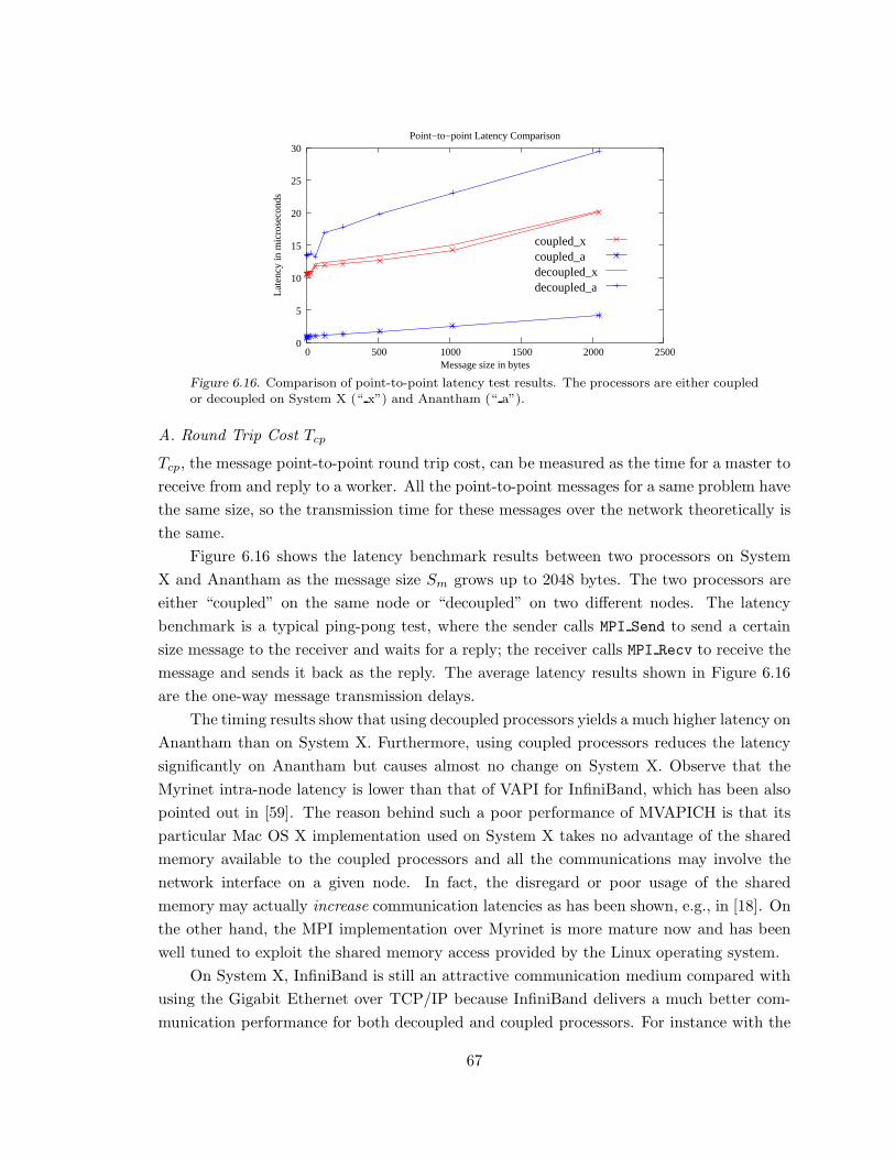
coupled_xcoupled_adecoupled_xdecoupled_a
0
5
10
15
20
25
30
0 500 1000 1500 2000 2500
Late
ncy
in m
icro
seco
nds
Message size in bytes
Point−to−point Latency Comparison
Figure 6.16. Comparison of point-to-point latency test results. The processors are either coupled
or decoupled on System X (“ x”) and Anantham (“ a”).
A. Round Trip Cost Tcp
Tcp, the message point-to-point round trip cost, can be measured as the time for a master to
receive from and reply to a worker. All the point-to-point messages for a same problem have
the same size, so the transmission time for these messages over the network theoretically is
the same.
Figure 6.16 shows the latency benchmark results between two processors on System
X and Anantham as the message size Sm grows up to 2048 bytes. The two processors are
either “coupled” on the same node or “decoupled” on two different nodes. The latency
benchmark is a typical ping-pong test, where the sender calls MPI Send to send a certain
size message to the receiver and waits for a reply; the receiver calls MPI Recv to receive the
message and sends it back as the reply. The average latency results shown in Figure 6.16
are the one-way message transmission delays.
The timing results show that using decoupled processors yields a much higher latency on
Anantham than on System X. Furthermore, using coupled processors reduces the latency
significantly on Anantham but causes almost no change on System X. Observe that the
Myrinet intra-node latency is lower than that of VAPI for InfiniBand, which has been also
pointed out in [59]. The reason behind such a poor performance of MVAPICH is that its
particular Mac OS X implementation used on System X takes no advantage of the shared
memory available to the coupled processors and all the communications may involve the
network interface on a given node. In fact, the disregard or poor usage of the shared
memory may actually increase communication latencies as has been shown, e.g., in [18]. On
the other hand, the MPI implementation over Myrinet is more mature now and has been
well tuned to exploit the shared memory access provided by the Linux operating system.
On System X, InfiniBand is still an attractive communication medium compared with
using the Gigabit Ethernet over TCP/IP because InfiniBand delivers a much better com-
munication performance for both decoupled and coupled processors. For instance with the
67
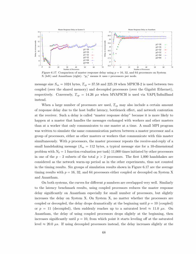
p1=16p2=16p1=32p2=32p1=64p2=64
2 7
8
9
10
11
12
13
14
10 20 30 40 50 60 70
Del
ay in
mic
rose
cond
s
Number of Processors
Master Response Delay on System X
p1=16p2=16p1=32p2=32p1=64p2=64
2
17
17.5
18
18.5
19
19.5
20
20.5
21
10 20 30 40 50 60 70
Del
ay in
mic
rose
cond
s
Number of Processors
Master Response Delay on Anantham
16.5
Figure 6.17. Comparison of master response delay using p = 16, 32, and 64 processors on System
X (left) and Anantham (right). “pi” means it uses i processors per node.
message size Sm = 1024 bytes, Tcp = 37.58 and 225.19 when MPICH-2 is used between two
coupled (over the shared memory) and decoupled processors (over the Gigabit Ethernet),
respectively. Conversely, Tcp = 14.26 µs when MVAPICH is used via VAPI/InfiniBand
instead.
When a large number of processors are used, Tcp may also include a certain amount
of response delay due to the host buffer latency, bottleneck effect, and network contention
at the receiver. Such a delay is called “master response delay” because it is more likely to
happen at a master that handles the messages exchanged with workers and other masters
than at a worker that only communicates to one master at a time. A small MPI program
was written to simulate the same communication pattern between a master processor and a
group of processors, either as other masters or workers that communicate with this master
simultaneously. With p processors, the master processor repeats the receive-and-reply of a
small handshaking message (Sm = 112 bytes, a typical message size for a 10-dimensional
problem with Nb = 1 function evaluation per task) 11,000 times initiated by other processors
in one of the p − 2 subsets of the total p > 2 processors. The first 1,000 handshakes are
considered as the network warm-up period as in the other experiments, thus not counted
in the timing results. Six groups of simulation results shown in Figure 6.17 are the average
timing results with p = 16, 32, and 64 processors either coupled or decoupled on System X
and Anantham.
On both systems, the curves for different p numbers are overlapped very well. Similarly
to the latency benchmark results, using coupled processors reduces the master response
delay significantly on Anantham especially for small number of processors, but slightly
increases the delay on System X. On System X, no matter whether the processors are
coupled or decoupled, the delay drops dramatically at the beginning until p = 10 (coupled)
or p = 11 (decoupled), then suddenly reaches up to a saturated level ≈ 11.0 µs. On
Anantham, the delay of using coupled processors drops slightly at the beginning, then
increases significantly until p = 10, from which point it starts leveling off at the saturated
level ≈ 20.0 µs. If using decoupled processors instead, the delay increases slightly at the
68

System XAnantham
2/e
0.02
0.04
0.06
0.08
0.1
0.12
0.14
0.16
0 10 20 30 40 50 60 70Processor Breakpoint
Comparison of Ratio R
Rat
io R
2 /e
Figure 6.18. Comparison of the ratio R2/e for different breakpoints of the piecewise Tcp model
on System X and Anantham.
0
50
100
150
200
250
300
350
400
−20 −10 0 10 20 30 40 50
Fre
quen
cy
Residual Error in microseconds
Histogram of Residuals
0
100
200
300
400
500
600
−80 −60 −40 −20 0 20 40 60
Fre
quen
cy
Residual Error in microseconds
Histogram of Residuals
Figure 6.19. Histogram of residual errors of the linear regression models for Tcp on System X
(left) and Anantham (right).
beginning from p = 2 to p = 4, then drops to a level ≈ 20.3 µs. The narrower bandwidth on
Anantham yields a longer delay because the network contention occurs when a large number
of processors are communicating to each other simultaneously. In the following experiments,
coupled processors are used primarily because the cluster is utilized more efficiently (when
decoupled processors are used, 50% of the processors are idle). Secondarily, it makes a
minor difference on System X and even reduces the latency on Anantham.
The above experiments conclude that the Tcp between a master and a group of proces-
sors is affected by two factors: (1) the message size Sm and (2) the number of processors p
that communicate with the master. Tcp increases as Sm grows, but varies when p is small
and levels off at a certain value when p is sufficiently large depending on computing system.
Therefore, Tcp is formed as a multivariate function of Sm and p as follows:
Tcp(p, Sm) = TL(Sm) + Td(p),
where TL(Sm) is defined as the point-to-point latency function in terms of Sm without the
response delay and Td(p) as the pure response delay function in terms of p. In Figure 6.16,
69
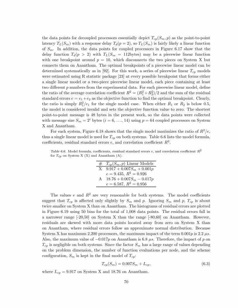
the data points for decoupled processors essentially depict Tcp(Sm, p) as the point-to-point
latency TL(Sm) with a response delay Td(p = 2), so TL(Sm) is fairly likely a linear function
of Sm. In addition, the data points for coupled processors in Figure 6.17 show that the
delay function Td(p > 2) with TL(Sm = 112bytes) may be a piecewise linear function
with one breakpoint around p = 10, which disconnects the two pieces on System X but
connects them on Anantham. The optimal breakpoints of a piecewise linear model can be
determined systematically as in [92]. For this work, a series of piecewise linear Tcp models
were estimated using R statistic package [23] at every possible breakpoint that forms either
a single linear model or a two-piece piecewise linear model, each piece containing at least
two different p numbers from the experimental data. For each piecewise linear model, define
the ratio of the average correlation coefficient R2 = (R21 +R2
2)/2 and the sum of the residual
standard errors e = e1+e2 as the objective function to find the optimal breakpoint. Clearly,
the ratio is simply R21/e1 for the single model case. When either R1 or R2 is below 0.5,
the model is considered invalid and sets the objective function value to zero. The shortest
point-to-point message is 48 bytes in the present work, so the data points were collected
with message size Sm = 2i bytes (i = 6, . . ., 14) using p = 64 coupled processors on System
X and Anantham.
For each system, Figure 6.18 shows that the single model maximizes the ratio of R2/e,
thus a single linear model is used for Tcp on both systems. Table 6.6 lists the model formula,
coefficients, residual standard errors e, and correlation coefficient R2.
Table 6.6. Model formula, coefficients, residual standard errors e, and correlation coefficient R2
for Tcp on System X (X) and Anantham (A).
# Tcp(Sm, p) Linear ModelsX 9.917 + 0.007Sm + 0.001p
e = 9.435, R2 = 0.926A 18.76 + 0.007Sm − 0.017p
e = 6.587, R2 = 0.956
The values e and R2 are very reasonable for both systems. The model coefficients
suggest that Tcp is affected only slightly by Sm and p. Ignoring Sm and p, Tcp is about
twice smaller on System X than on Anantham. The histograms of residual errors are plotted
in Figure 6.19 using 50 bins for the total of 1,008 data points. The residual errors fall in
a narrower range [-20,50] on System X than the range [-80,60] on Anantham. However,
residuals are skewed with more data points located away from zero on System X than
on Anantham, where residual errors follow an approximate normal distribution. Because
System X has maximum 2,200 processors, the maximum impact of the term 0.001p is 2.2 µs.
Also, the maximum value of −0.017p on Anantham is 6.8 µs. Therefore, the impact of p on
Tcp is negligible on both systems. Since the factor Sm has a large range of values depending
on the problem dimension, the number of function evaluations per node, and the scheme
configuration, Sm is kept in the final model of Tcp:
Tcp(Sm) = 0.007Sm + Lcp, (6.3)
where Lcp = 9.917 on System X and 18.76 on Anantham.
70

100
200
300
400
500
600
700
0 2000 4000 6000 8000 10000 12000 14000 16000 18000
Late
ncy
in m
icro
seco
nds
Message Size in bytes
Broadcast Latency Comparison
Anatham
System X
0
100
200
300
400
500
600
700
800
0 20 40 60 80 100 120 140
Late
ncy
in m
icro
seco
nds
Number of Processors
Broadcast Latency with Message Size=16384 bytes
AnanthamSystem X
Figure 6.20. Comparison of broadcast latency results (in microseconds) on System X and Anan-tham. (a) The message size increases with p = 32 coupled processor nodes (left). (b) A fixed
size message (Sm=16K bytes) is broadcast on an increasing number of processors p = 2, . . . , 128
(right).
2/e
System XAnantham
Rat
io R
2 /e
0
0.002
0.004
0.006
0.008
0.01
0.012
0 10 20 30 40 50 60Processor Breakpoint
Comparison of Ratio R
Figure 6.21. Comparison of the ratio R2/e for different breakpoints of the piecewise Tca model
on System X and Anantham.
B. Broadcast Cost Tca
Tca measures the global one-to-all communication cost among master processors that col-
laborate on the parallel Selection, one of the main steps of the DIRECT algorithm. From
the second iteration, the associated global operations occur in the following five phases:
1. BARRIER: All masters prepare local convex hull boxes and counters, then wait
at a barrier.
2. GATHER I: The root master m0 gathers the counters of the local convex hull
boxes to prepare the buffer.
3. GATHER II: m0 gathers the local convex hull boxes to the buffer.
4. BCAST I: m0 broadcasts the counter of the global convex hull boxes.
5. BCAST II: m0 broadcasts the global convex hull boxes.
Essentially, BARRIER can be approximated as an all-to-one GATHER followed by
an one-to-all BCAST operations for a small message. The complexity and efficiency of
these global operations in different MPI implementations depend on the chosen algorithms.
71
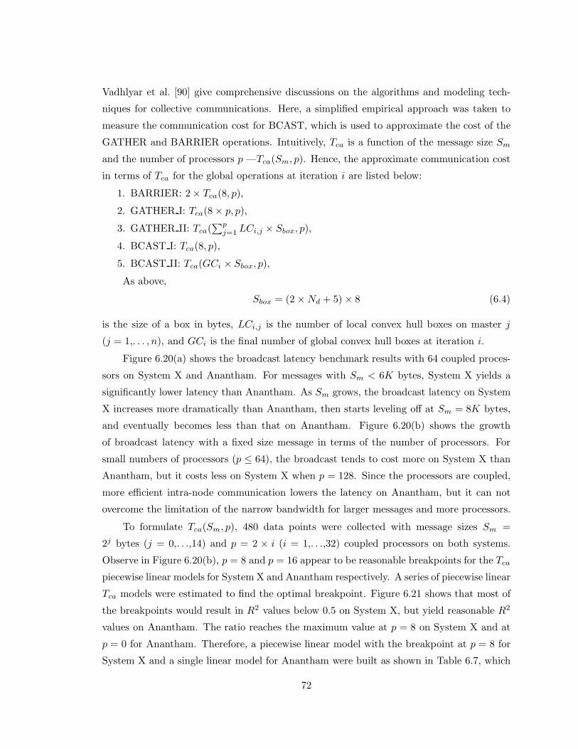
Vadhlyar et al. [90] give comprehensive discussions on the algorithms and modeling tech-
niques for collective communications. Here, a simplified empirical approach was taken to
measure the communication cost for BCAST, which is used to approximate the cost of the
GATHER and BARRIER operations. Intuitively, Tca is a function of the message size Sm
and the number of processors p —Tca(Sm, p). Hence, the approximate communication cost
in terms of Tca for the global operations at iteration i are listed below:
1. BARRIER: 2 × Tca(8, p),
2. GATHER I: Tca(8 × p, p),
3. GATHER II: Tca(∑p
j=1 LCi,j × Sbox, p),
4. BCAST I: Tca(8, p),
5. BCAST II: Tca(GCi × Sbox, p),
As above,
Sbox = (2 × Nd + 5) × 8 (6.4)
is the size of a box in bytes, LCi,j is the number of local convex hull boxes on master j
(j = 1,. . . , n), and GCi is the final number of global convex hull boxes at iteration i.
Figure 6.20(a) shows the broadcast latency benchmark results with 64 coupled proces-
sors on System X and Anantham. For messages with Sm < 6K bytes, System X yields a
significantly lower latency than Anantham. As Sm grows, the broadcast latency on System
X increases more dramatically than Anantham, then starts leveling off at Sm = 8K bytes,
and eventually becomes less than that on Anantham. Figure 6.20(b) shows the growth
of broadcast latency with a fixed size message in terms of the number of processors. For
small numbers of processors (p ≤ 64), the broadcast tends to cost more on System X than
Anantham, but it costs less on System X when p = 128. Since the processors are coupled,
more efficient intra-node communication lowers the latency on Anantham, but it can not
overcome the limitation of the narrow bandwidth for larger messages and more processors.
To formulate Tca(Sm, p), 480 data points were collected with message sizes Sm =
2j bytes (j = 0,. . .,14) and p = 2 × i (i = 1,. . .,32) coupled processors on both systems.
Observe in Figure 6.20(b), p = 8 and p = 16 appear to be reasonable breakpoints for the Tca
piecewise linear models for System X and Anantham respectively. A series of piecewise linear
Tca models were estimated to find the optimal breakpoint. Figure 6.21 shows that most of
the breakpoints would result in R2 values below 0.5 on System X, but yield reasonable R2
values on Anantham. The ratio reaches the maximum value at p = 8 on System X and at
p = 0 for Anantham. Therefore, a piecewise linear model with the breakpoint at p = 8 for
System X and a single linear model for Anantham were built as shown in Table 6.7, which
72
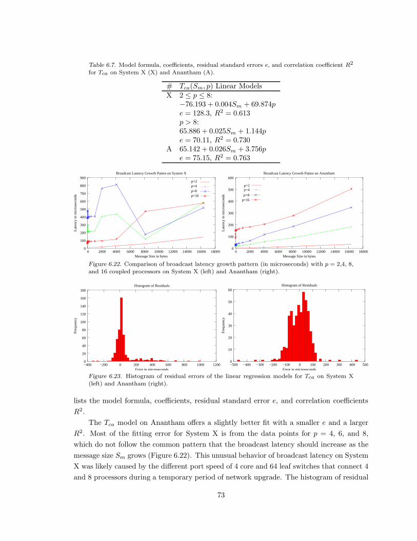
Table 6.7. Model formula, coefficients, residual standard errors e, and correlation coefficient R2
for Tca on System X (X) and Anantham (A).
# Tca(Sm, p) Linear ModelsX 2 ≤ p ≤ 8:
−76.193 + 0.004Sm + 69.874pe = 128.3, R2 = 0.613p > 8:65.886 + 0.025Sm + 1.144pe = 70.11, R2 = 0.730
A 65.142 + 0.026Sm + 3.756pe = 75.15, R2 = 0.763
0
100
200
300
400
500
600
700
800
900
0 2000 4000 6000 8000 10000 12000 14000 16000 18000
Late
ncy
in m
icro
seco
nds
Message Size in bytes
Broadcast Latency Growth Patten on System X
p=16
p=4p=8
p=2
0
100
200
300
400
500
600
0 2000 4000 6000 8000 10000 12000 14000 16000 18000
Late
ncy
in m
icro
seco
nds
Message Size in bytes
Broadcast Latency Growth Patten on Anantham
p=16p=8
p=4p=2
Figure 6.22. Comparison of broadcast latency growth pattern (in microseconds) with p = 2,4, 8,
and 16 coupled processors on System X (left) and Anantham (right).
0
20
40
60
80
100
120
140
160
180
−400 −200 0 200 400 600 800 1000 1200
Fre
quen
cy
Error in microseconds
Histogram of Residuals
0
10
20
30
40
50
60
−500 −400 −300 −200 −100 0 100 200 300 400 500
Fre
quen
cy
Error in microseconds
Histogram of Residuals
Figure 6.23. Histogram of residual errors of the linear regression models for Tca on System X
(left) and Anantham (right).
lists the model formula, coefficients, residual standard error e, and correlation coefficients
R2.
The Tca model on Anantham offers a slightly better fit with a smaller e and a larger
R2. Most of the fitting error for System X is from the data points for p = 4, 6, and 8,
which do not follow the common pattern that the broadcast latency should increase as the
message size Sm grows (Figure 6.22). This unusual behavior of broadcast latency on System
X was likely caused by the different port speed of 4 core and 64 leaf switches that connect 4
and 8 processors during a temporary period of network upgrade. The histogram of residual
73
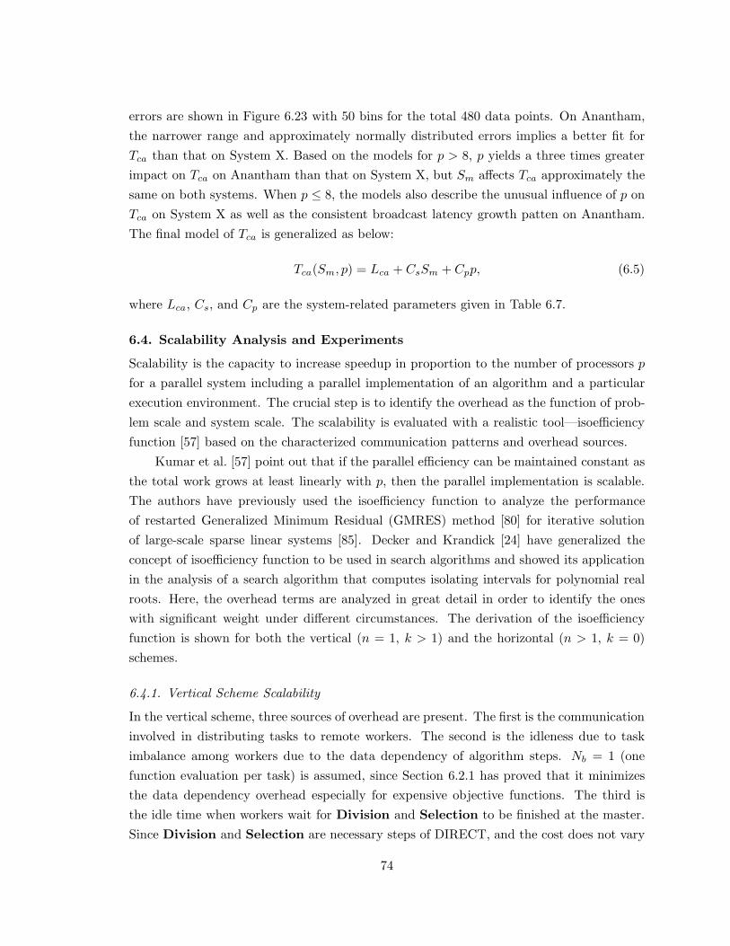
errors are shown in Figure 6.23 with 50 bins for the total 480 data points. On Anantham,
the narrower range and approximately normally distributed errors implies a better fit for
Tca than that on System X. Based on the models for p > 8, p yields a three times greater
impact on Tca on Anantham than that on System X, but Sm affects Tca approximately the
same on both systems. When p ≤ 8, the models also describe the unusual influence of p on
Tca on System X as well as the consistent broadcast latency growth patten on Anantham.
The final model of Tca is generalized as below:
Tca(Sm, p) = Lca + CsSm + Cpp, (6.5)
where Lca, Cs, and Cp are the system-related parameters given in Table 6.7.
6.4. Scalability Analysis and Experiments
Scalability is the capacity to increase speedup in proportion to the number of processors p
for a parallel system including a parallel implementation of an algorithm and a particular
execution environment. The crucial step is to identify the overhead as the function of prob-
lem scale and system scale. The scalability is evaluated with a realistic tool—isoefficiency
function [57] based on the characterized communication patterns and overhead sources.
Kumar et al. [57] point out that if the parallel efficiency can be maintained constant as
the total work grows at least linearly with p, then the parallel implementation is scalable.
The authors have previously used the isoefficiency function to analyze the performance
of restarted Generalized Minimum Residual (GMRES) method [80] for iterative solution
of large-scale sparse linear systems [85]. Decker and Krandick [24] have generalized the
concept of isoefficiency function to be used in search algorithms and showed its application
in the analysis of a search algorithm that computes isolating intervals for polynomial real
roots. Here, the overhead terms are analyzed in great detail in order to identify the ones
with significant weight under different circumstances. The derivation of the isoefficiency
function is shown for both the vertical (n = 1, k > 1) and the horizontal (n > 1, k = 0)
schemes.
6.4.1. Vertical Scheme Scalability
In the vertical scheme, three sources of overhead are present. The first is the communication
involved in distributing tasks to remote workers. The second is the idleness due to task
imbalance among workers due to the data dependency of algorithm steps. Nb = 1 (one
function evaluation per task) is assumed, since Section 6.2.1 has proved that it minimizes
the data dependency overhead especially for expensive objective functions. The third is
the idle time when workers wait for Division and Selection to be finished at the master.
Since Division and Selection are necessary steps of DIRECT, and the cost does not vary
74

with k, the third source of overhead is considered as a constant for a particular problem
with a specified stopping condition.
Let W be the total number of function evaluations over Imax iterations,
W =
Imax∑
i=1
Fi, (6.6)
where Fi denotes all the function evaluation tasks at iteration i. The total overhead for k
workers is
To(W,k) = k × Tk − W × Tf , (6.7)
where Tk is the parallel execution time with k workers. Define the parallel efficiency Ep as
Ep =W × Tf
k × Tk
. (6.8)
If Ep can be maintained constant as W grows at least linearly with k, then the vertical
scheme is scalable. The isoefficiency function is derived from Equation (6.7) and (6.8) as
follows:
W =Ep
1 − Ep
× (To(W,k)/Tf ). (6.9)
It describes the total work W in terms of To, the total overhead function given a desired Ep
and the constant objective function cost Tf . To find if W is a linear function of k, To(W,k)
as a function of W needs to be extended by accumulating over all Imax iterations. All the
costs, except for the function evaluation, are included in To(W,k). So it has three terms:
T 1oc (communication overhead), Tod (data dependency overhead), and a constant Tos (the
Division and Selection cost).
The interaction between masters and workers is described in full detail in Section 4.1.2.
Here, the communication phases are only outlined.
(1) Each of k workers sends a non-blocking request to a random selected master.
(2) For each worker that has sent a non-blocking request or that is in the queue,
a master sends a task if any. If no more tasks, the master sends a “no point”
message, or if no more iterations, sends a “all done” message.
(3) The workers who received tasks send values back to the master. Those who re-
ceived the “no point” notice check with other masters, who may have tasks, and
if none have tasks, send blocking requests and wait. Those who received the “all
done” notice terminate. For each value received, a master sends a task if any; If
no more tasks, sends a “no point” notice; For each blocking request, queues up
the worker.
Only one master distributes tasks, so if it runs out of tasks at the end of an iteration,
all workers will block waiting in its queue. So, Phase (1) happens only at the first iteration
75

GRQUROSCMIFEBY
0
1000
2000
3000
4000
5000
6000
7000
0 10 20 30 40 50 60 70 80 90 100
Idle
Cyc
les
Number of Workers
Worker Idle Cycles
GRQUROSCMIFEBY
0
2000
4000
6000
8000
10000
12000
14000
16000
0 20 40 60 80 100 120 140
Num
ber
of E
valu
atio
ns
Number of Iterations
Function Evaluation Tasks per Iteration
Figure 6.24. All the worker idle cycles, shown in (a) on the left, are calculated using k = 2, . . .,100 workers and the function evaluations are shown in (b) on the right for all the test problems
on System X. Imax = 122.
because the workers are all in the queue of the master from the second iteration. Phases (2)
and (3) are repeated at every iteration. To sum up the communication overhead, consider
the message types and the frequency of these messages exchanged between a master and a
group of workers:
(a) T1 = k × Tcp/2 (k workers send nonblocking requests),
(b) T2 = Fi × Tcp/2 (workers receive Fi tasks),
(c) T3 = Fi × Tcp/2 + k × Tcp (the master receives all function values and sends
“no point” messages at end of each iteration to k workers; all workers then send
blocking requests to the master),
(d) T4 = k × Tcp/2 (workers receive “all done” messages from the master at the last
iteration).
The communication overhead over all iterations is
T 1oc = T1 +
Imax∑
i
T2 +
Imax∑
i
T3 + T4.
Represent it as a function of W (Equation 6.6) and k with Tcp(Sm) (Equation 6.3):
T 1oc(W,k) = (k(1 + Imax) + W )Tcp(Sm)
= (0.007Sm + Lcp)W
+ (1 + Imax)(0.007Sm + Lcp)k.
(6.10)
For point-to-point messages, the message size Sm (in bytes) depends on the problem di-
mension Nd:
Sm = (Nd + 4) × 8. (6.11)
Therefore, Tcp(Sm) is a constant for the same problem on a particular system. Because T 1oc
depends linearly on k, it grows linearly as O(k) for a fixed size problem specified by Imax
and W . On System X, the twice smaller Lcp (Table 6.6) gives a slower growth of T 1oc in
terms of k than that on Anantham.
76

GRQUROSCMIFEBY
−1500
−1000
−500
0
500
1000
1500
0 10 20 30 40 50 60 70 80 90 100
Idle
Cyc
les
Number of Workers
Residual Scatter Plot
Figure 6.25. The scatter plot of residuals δp(k) for test problems on System X.
The second source of overhead—data dependency—is as important as the communi-
cation. It causes task imbalance among workers. At iteration i, if some workers obtain no
tasks, when the number of tasks Fi is less than the number of workers k, or obtain fewer
tasks than others, idle cycles will appear, each of which lasts about Tf . The number Xi of
such cycles can be derived from the equation:
δi+ × (k − Xi) + δi− × (Xi) = Fi,
where δi+ = ⌈Fi/k⌉ and δi− = ⌊Fi/k⌋ are the workers’ task shares defined in the workload
model of Section 6.2.2. Because δi+ − δi− = 1,
Xi =δi+ × k − Fi
δi+ − δi−
= δi+ × k − Fi,
yielding the total data dependency overhead:
Tod =
Imax∑
i
Xi × Tf
=
Imax∑
i
(
⌈
Fi
k
⌉
× k − Fi)Tf .
(6.12)
Observe that Tod becomes 0 when Fi is a multiple of k. Figure 6.24(a) shows the results
for∑Imax
i=1 (Xi,j), which is the total number of worker idle cycles over Imax iterations using
j = 2,. . ., k workers.
Interestingly, each curve for the total idle cycles presents a linear function of k with a
fluctuation, which falls in a larger range when more workers are used. Note that the wall
clock duration of data dependency overhead is actually
Imax∑
i=1
sgn(Xi,j)Tf ≥Imax∑
i=1
(Xi,j)Tf/k,
77

Table 6.8. Comparison of the growth rate θ, the residual standard error e, and the correlation
coefficient R2 for the estimated linear growth of the worker idle cycles for test problems.
# θ e R2
GR 61.093 327.6 0.966QU 60.724 202.5 0.986RO 61.816 194.1 0.988SC 61.879 200.1 0.987MI 59.186 241.2 0.980FE 64.613 234.9 0.984BY 60.658 269.7 0.976
and this average—rather than total—overhead per worker and is considered for experimental
verification here.
The growth rate of the number of idle cycles was estimated by the same linear regression
tool used in the previous subsection. Although the QU, SC, and MI problems generate
more function evaluation tasks per iteration than other problems do so (Figure 6.24(b)),
the growth rates are very close to each other for these test problems as shown in Table 6.8.
Hence, Tod grows approximately linearly with k with a fluctuation that can be described
by the residual error function δp(k) (Figure 6.25).
Table 6.9. Comparison of Cm, Txoc/k (on System X), Ta
oc/k (on Anantham), and Tod/k (in
seconds) for all test problems using k = 99 workers. Imax = 122 with first 12 iterations skipped
for estimation. Nb = 1. Nd = 150 and Tf = 0.1 for artificial functions, Nd = 16 and Tf = 2.66
for FE, and Nd = 143 and Tf = 11.02 for BY.
# Cm T xoc/k T a
oc/k Tod/k
GR 413332 0.039 0.057 4.450QU 1598908 0.149 0.221 5.371RO x 1021480 0.097 – 5.101RO a 1017544 – 0.141 5.540SC 1487836 0.139 0.206 5.368MI 1508052 0.141 0.209 4.957FE 59604 – 0.006 156.860BY 528468 0.048 – 616.790
Table 6.9 compares the number of one-way messages Cm, the theoretical communication
overheads per worker T xoc/k and T a
oc/k on System X and Anantham, respectively, and the
wall clock data dependency overhead Tod/k for all test problems with k = 99 workers.
On both System X and Anantham, Imax = 122 iterations were run, such that the first 12
iterations skipped, so the number of one-way messages is Cm = 2(k(Imax −12)+∑Imax
i=13 Fi).
Both T xoc and T a
oc were estimated using the formula for T 1oc in Equation 6.10 given Cm, Fi
(the number of function evaluation tasks per iteration collected from the runs), the linear
78
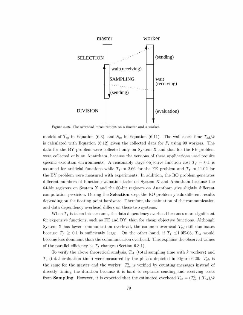
SAMPLING(receiving)
wait(receiving)
SELECTION
master worker
(sending)
DIVISION (evaluation)
(sending)
wait
Figure 6.26. The overhead measurement on a master and a worker.
models of Tcp in Equation (6.3), and Sm in Equation (6.11). The wall clock time Tod/k
is calculated with Equation (6.12) given the collected data for Fi using 99 workers. The
data for the BY problem were collected only on System X and that for the FE problem
were collected only on Anantham, because the versions of these applications used require
specific execution environments. A reasonably large objective function cost Tf = 0.1 is
assumed for artificial functions while Tf ≈ 2.66 for the FE problem and Tf ≈ 11.02 for
the BY problem were measured with experiments. In addition, the RO problem generates
different numbers of function evaluation tasks on System X and Anantham because the
64-bit registers on System X and the 80-bit registers on Anantham give slightly different
computation precision. During the Selection step, the RO problem yields different results
depending on the floating point hardware. Therefore, the estimation of the communication
and data dependency overhead differs on these two systems.
When Tf is taken into account, the data dependency overhead becomes more significant
for expensive functions, such as FE and BY, than for cheap objective functions. Although
System X has lower communication overhead, the common overhead Tod still dominates
because Tf ≥ 0.1 is sufficiently large. On the other hand, if Tf ≤1.0E-03, Tod would
become less dominant than the communication overhead. This explains the observed values
of the parallel efficiency as Tf changes (Section 6.3.1).
To verify the above theoretical analysis, Tsk (total sampling time with k workers) and
Te (total evaluation time) were measured by the phases depicted in Figure 6.26. Tsk is
the same for the master and the worker. T 1oc is verified by counting messages instead of
directly timing the duration because it is hard to separate sending and receiving costs
from Sampling. However, it is expected that the estimated overhead Tot = (T 1oc + Tod)/k
79

Table 6.10. The experimental results of the Sampling cost Tsk and the evaluation cost Te for
all test problems on System X (‘ x’) and Anantham (‘ a’). The combined experimental overhead
Toe = Tsk − Te/k is compared to the estimated overhead Tot = (T 1oc + Tod)/k.
# Tsk Te Toe Cm Tot
GR x 202.44 19578.0 4.68 413332 4.50GR a 203.28 19578.0 5.52 413332 4.51QU x 802.48 78857.0 5.94 1598908 5.52QU a 803.73 78858.0 7.18 1598908 5.59RO x 510.46 49987.0 5.54 1021480 5.20RO a 509.65 49789.0 6.73 1017544 5.68SC x 746.46 73306.0 5.99 1487836 5.51SC a 748.85 73304.0 8.41 1487836 5.57MI x 756.44 74316.0 5.77 1508052 5.10MI a 757.83 74316.0 7.16 1508052 5.17FE a 696.25 50608.0 185.06 59604 156.87BY x 29179.0 2788790 1009.40 528468 616.84
(the sum of the theoretical communication and data dependency overhead per worker in
Table 6.9) should be approximately equal to the experimental result Toe = Tsk − Te/k as
listed in Table 6.10.
The Sampling cost Tsk is approximately the same on both systems. Note that the
combined experimental overhead Toe is greater than the theoretical estimation Tot. More-
over, the scaled difference (Toe − Tot)/Tsk is larger on Anantham than that on System X.
Nevertheless, Cm matches exactly (Table 6.9) the experimental results. One possibility is
that the communication overhead could be underestimated because the small simulation
program that generated the data points for modeling Tcp may incur less overhead than
the full-size DIRECT optimization program does so with a large amount of memory allo-
cated. There might also exist another system-dependent source of overhead other than the
communication, such as memory access inefficiency, that may increase the overhead Toe on
Anantham.
With all the overhead terms analyzed, the isoefficiency function (Equation 6.9) for the
vertical scheme may be expressed as follows:
W =Ep
1 − Ep
× T 1oc(W,k) + Tod(k) + Tos
Tf
,
where T 1oc(k) is a linear function of k, Tod(k) is approximately linear function of k, and Tos
is a constant for a particular problem with specified Imax and resulting W . Therefore, W
becomes
W =Ep(Tcpk(1 + Imax) + Tod(k) + Tos)/Tf
1 − Ep − EpTcp/Tf
.
Firstly, observe that W grows linearly with k, meaning that the vertical scheme is scalable.
Secondly, a larger ratio of Tcp/Tf on a particular system requires a faster growth of W to
maintain the same Ep as more workers are used. Lastly, a larger Tf gives a better scalability.
80

GRQUROSCMI
0
100000
200000
300000
400000
500000
600000
700000
800000
900000
1e+06
0 5 10 15 20 25 30 35
Idle
Cyc
les
Number of Masters
Total Master Idle Cycles
Figure 6.27. The total master idle cycles are calculated with the data of Fi,j , the function
evaluations on master j at iteration i. n = 2, 4, . . ., 32 masters are used for test problems with
Imax = 122.
6.4.2. Horizontal Scheme Scalability
When the objective function is computationally cheap, the horizontal scheme is more suit-
able than the vertical scheme as discussed in Section 6.3.1. Thus, Tf ≈ 2.6E-05 was consid-
ered for all the artificial test problems in the scalability analysis of the horizontal scheme
with multiple masters (n > 1) and no workers (k = 0) in a single domain.
The overhead includes T 2oc, the communication overhead involved in the global convex
hull computation during the parallel Selection and T ′od, the data dependency overhead
among masters:
T ′o(H,W,n) = T 2
oc(H,n) + T ′od(H,W,n), (6.13)
where H stands for the total work in the convex hull computation.
Two components of T 2oc are (1) Tou, the point-to-point communication overhead for
updating the intermediate results and finalization, and (2) Toh, the collective communica-
tion overhead for the parallel Selection. The messages for intermediate data update and
termination process are from point to point using a fixed size buffer, thus
Tou(n) = (Imax +1
2)(n − 1)Tcp, (6.14)
where Tcp is a constant. Therefore, Tou(n) grows linearly with n regardless of systems. The
global collective communication is approximated with five phases and six messages from
the second iteration as discussed in Section 6.3.2, thus
Toh =
Imax−1∑
i
[3Tca(8, n) + Tca(8n, n)
+ Tca(
n∑
j=1
LCi,j × Sbox, n)
+ Tca(GCi × Sbox, n)].
(6.15)
All terms of Toh grow linearly in O(n).
81
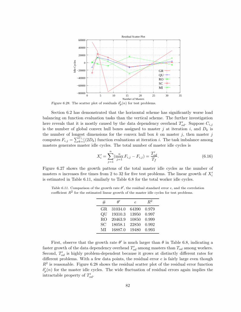
GRQUROSCMI
−80000
−60000
−40000
−20000
0
20000
40000
60000
0 5 10 15 20 25 30 35
Idle
Cyc
les
Number of Masters
Residual Scatter Plot
Figure 6.28. The scatter plot of residuals δ′p(n) for test problems.
Section 6.2 has demonstrated that the horizontal scheme has significantly worse load
balancing on function evaluation tasks than the vertical scheme. The further investigation
here reveals that it is mostly caused by the data dependency overhead T ′od. Suppose Ci,j
is the number of global convex hull boxes assigned to master j at iteration i, and Dk is
the number of longest dimensions for the convex hull box k on master j, then master j
computes Fi,j =∑Ci,j
k=1(2Dk) function evaluations at iteration i. The task imbalance among
masters generates master idle cycles. The total number of master idle cycles is
X ′i =
n∑
j=1
(n
maxj=1
Fi,j − Fi,j) =T ′
od
Tf
. (6.16)
Figure 6.27 shows the growth pattens of the total master idle cycles as the number of
masters n increases five times from 2 to 32 for five test problems. The linear growth of X ′i
is estimated in Table 6.11, similarly to Table 6.8 for the total worker idle cycles.
Table 6.11. Comparison of the growth rate θ′, the residual standard error e, and the correlation
coefficient R2 for the estimated linear growth of the master idle cycles for test problems.
# θ′ e R2
GR 31034.0 64390 0.979QU 19310.3 13950 0.997RO 20463.9 10850 0.999SC 18058.1 22850 0.992MI 16887.0 19480 0.993
First, observe that the growth rate θ′ is much larger than θ in Table 6.8, indicating a
faster growth of the data dependency overhead T ′od among masters than Tod among workers.
Second, T ′od is highly problem-dependent because it grows at distinctly different rates for
different problems. With a few data points, the residual error e is fairly large even though
R2 is reasonable. Figure 6.28 shows the residual scatter plot of the residual error function
δ′p(n) for the master idle cycles. The wide fluctuation of residual errors again implies the
intractable property of T ′od.
82
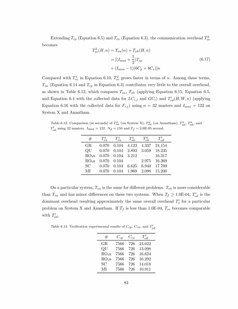
Extending Tcp (Equation 6.5) and Tca (Equation 6.3), the communication overhead T 2oc
becomes
T 2oc(H,n) = Tou(n) + Toh(H,n)
= [(Imax +1
2)Tcp
+ (Imax − 1)(6Cp + 8Cs)]n
(6.17)
Compared with T 1oc in Equation 6.10, T 2
oc grows faster in terms of n. Among these terms,
Tou (Equation 6.14 and Tcp in Equation 6.3) contributes very little to the overall overhead,
as shown in Table 6.12, which compares Tou, Toh (applying Equation 6.15, Equation 6.5,
and Equation 6.4 with the collected data for LCi,j and GCi) and T ′od(H,W,n) (applying
Equation 6.16 with the collected data for Fi,j) using n = 32 masters and Imax = 122 on
System X and Anantham.
Table 6.12. Comparison (in seconds) of Txou (on System X), Ta
ou (on Anantham), Txoh
, Taoh
, and
T ′od
using 32 masters. Imax = 122. Nd = 150 and Tf = 2.6E-05 second.
# T xou T a
ou T xoh T a
oh T ′od
GR 0.070 0.104 4.123 4.337 24.154QU 0.070 0.104 2.893 3.059 18.235RO x 0.070 0.104 3.212 – 16.317RO a 0.070 0.104 – 2.975 16.369SC 0.070 0.104 6.625 6.940 17.709MI 0.070 0.104 1.969 2.098 15.200
On a particular system, Tou is the same for different problems. Toh is more considerable
than Tou and has minor differences on these two systems. When Tf ≥ 1.0E-04, T ′od is the
dominant overhead resulting approximately the same overall overhead T ′o for a particular
problem on System X and Anantham. If Tf is less than 1.0E-04, Toc becomes comparable
with T ′od.
Table 6.13. Verification experimental results of Ccp, Cca, and T ′od
.
# Ccp Cca T ′od
GR 7566 726 24.622QU 7566 726 13.098RO x 7566 726 16.624RO a 7566 726 16.292SC 7566 726 14.018MI 7566 726 10.911
83

Several experiments were conducted using 32 masters (coupled processors on System X
and Anantham) to verify the above estimation. On the root master, two messages counters
Ccp and Cca were used to keep track of the point-to-point one-way messaging during the
intermediate update and the collective messaging during the Selection step respectively
for all the test runs. The Sampling cost Tsi on each of i = 1,. . .,32 masters were measured.
The experimental measurement of T ′od =
∑32i (max32
i Tsi − Tsi) is expected to be close to
the theoretical results in Table 6.12. Table 6.13 lists the experimental results of Ccp, Cca,
and T ′od.
Both Ccp and Cca were collected on the root master. Generally, Ccp = 2Imax(n−1)+2
and Cca = 6(Imax −1), where n = 32 and Imax = 122. Another n−3 oneway messages were
not counted by Ccp, because they were sent among non-root masters during final termi-
nation. Cca exactly matches the number of global messages for collective communication.
The experimental results for T ′od are close to the estimation especially for the GR and RO
problems.
Derived from Equation (6.9), the isoefficiency function for the horizontal scheme is
W =Ep
1 − Ep
× T 2oc(H,n) + T ′
od(H,W,n)
Tf
,
where T 2oc(H,n) is a linear function of n and T ′
od(H,W,n) is approximately a linear function
of n. Because the horizontal scheme has a faster growth rate of both communication over-
head and data dependency overhead, its scalability is worse than that of the vertical scheme.
Remarkably, the data dependency is not only a dominant source of overhead for expensive
objective functions, it is also highly problem-dependent and intractable. Furthermore, the
difference in communication characteristics on System X and Anantham has little impact
for expensive objective functions, but becomes considerable when the objective function
cost Tf is low.
6.4.3. Scalability Experiments
Empirical studies on scalability were done for all five benchmark functions with a fixed cost
Tf = 0.1, a growing problem dimension N = 2i (i = 2, . . ., 6), and an increasing number
of processors p = 10 · 2i−1 (i = 1, . . ., 5). Since the problem structure changes as N grows,
the traditionally defined scaled speedup is not applicable here. Since Tf is maintained
approximately constant by using a microsecond precision utility function gettimeofday in
C, the increase from 0.1 to the average cost per evaluation Te = pTp/Ne can be considered
84

4 8 16 6432 Problem Dimension N
0.1
0.12
0.14
0.16
0.18
0.2
0.22
0 40 60 80 100 120 140 160
Ave
rage
Cos
t per
Eva
luat
ion
ROGRQUSCMI
Comparison of Average Cost per Evaluation as N and p Grow
20Number of Processors p
Figure 6.29. The growth of Te as N and p increase for all five benchmark functions.
as the average overhead per function evaluation as both N and p increase, where Tp is the
parallel execution time with p processors and Ne is the actual number of evaluations.
Figure 6.29 plots how Te changes as N and p grow. For most problems, Te grows
slowly until N reaches 32 and p reaches 80. The larger increase in overhead for the QU
problem could be related to its special problem structure that causes more worker idleness
and computation during Selection and Division. Moreover, the growth in N may not
produce more concurrent evaluation tasks proportionally. Therefore, doubling p every time
when N is doubled is not guaranteed to maintain efficient performance. On the other hand,
load balancing can be improved greatly for a fixed p as N and the iteration limit Imax or
the evaluation limit Le grows. An experiment in Section 6.1.2 has shown that the parallel
efficiency curves for 100 processors reach more than 90%, 80%, and 70% when Imax = 30,
20, and 10, respectively, as N increases from 10 to 50, 100, and 150 for the problem RO
with the same cost Tf = 0.1.
The next scalability study varies the evaluation limit Le as p grows for the problems FE
and BY. The comparisons were also done with the number of iterations/evaluations fixed as
p grows. The fixed speedup and scaled speedup are plotted in Figure 6.30. The fixed speedup
follows the conventional definition Sf = T (W, 1)/T (W,p), where W is the fixed work load,
T (W, 1) is the execution time on a single processor, and T (W,p) is the parallel execution
time on p processors. The scaled speedup is usually obtained as Ss = p T (Ws, 1)/T (pWs, p),
where Ws is the base work for a single processor, T (Ws, 1) is the execution time with a single
processor on the work Ws, and T (pWs, p) is the parallel execution time with p processors
and the linearly increased work pWs. Ss needs to be redefined here because the stopping
condition MAX EVL is checked after all convex hull boxes have been sampled and subdivided,
meaning the number of evaluations does not grow exactly linearly as DIRECT iterates.
Therefore, define
Ss =p T (Ws, 1)
T (Wp, p)(pWs/Wp),
85
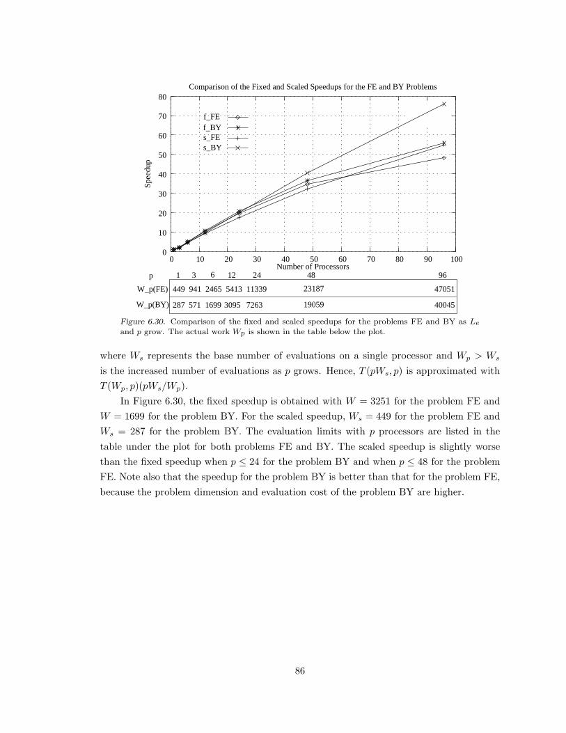
287 571 1699 3095 7263 19059 40045
449 941 2465 5413 11339 23187 47051W_p(FE)
W_p(BY)
p
f_FE
s_FEf_BY
s_BY
0 10 20 30 40 50 60 70 80 90 100 0
10
20
30
40
50
60
70
80
Spe
edup
Comparison of the Fixed and Scaled Speedups for the FE and BY Problems
Number of Processors 1 3 12 6 24 48 96
Figure 6.30. Comparison of the fixed and scaled speedups for the problems FE and BY as Le
and p grow. The actual work Wp is shown in the table below the plot.
where Ws represents the base number of evaluations on a single processor and Wp > Ws
is the increased number of evaluations as p grows. Hence, T (pWs, p) is approximated with
T (Wp, p)(pWs/Wp).
In Figure 6.30, the fixed speedup is obtained with W = 3251 for the problem FE and
W = 1699 for the problem BY. For the scaled speedup, Ws = 449 for the problem FE and
Ws = 287 for the problem BY. The evaluation limits with p processors are listed in the
table under the plot for both problems FE and BY. The scaled speedup is slightly worse
than the fixed speedup when p ≤ 24 for the problem BY and when p ≤ 48 for the problem
FE. Note also that the speedup for the problem BY is better than that for the problem FE,
because the problem dimension and evaluation cost of the problem BY are higher.
86

CHAPTER 7: Real World Applications
Like other global optimization approaches of [26] and [32], DIRECT is being tested
by parameter estimation for high dimensional nonlinear models. Moles et al. [68] applied
DIRECT to a global nonlinear parameter estimation problem in systems biology. However,
unnecessary overhead and complexity caused by inefficient implementation inside other
software packages (e.g., Matlab) may obscure DIRECT’s advanced features. Some compu-
tational biologists are attracted by DIRECT’s unique strategy of balancing global and local
search, its selection rules for potentially optimal regions according to a Lipschitz condition,
and its easy-to-use black box interface.
The JigCell systems biology project [3] at Virginia Tech is such an example of applying
DIRECT to a problem solving environment. Both global and local optimization techniques
are used for biological pathway modeling. One of the most important tools developed
for JigCell is the Parameter Estimator, which finds the optimal set of parameters to fit a
mathematical pathway model to experimental data.
Section 7.1 describes the general modeling process and Section 7.2 discusses primitive
optimization results from the work in [39]. More details and discussions can be found in
the work done by Panning et al. [74] and Zwolak et al. [99].
7.1. Cell Cycle Modeling in Systems Biology
The ultimate goal of molecular cell biology is to understand how the information stored in
the genome is read out and put into action as the physiological behavior of a living cell.
At one end of this continuum, genes direct the synthesis of polypeptide chains, and at the
other end, networks of interacting proteins govern how a cell moves, feeds, responds, and
reproduces. The model presented here is of the latter type and can be represented as a
system of ordinary differential equations (ODE).
The complexity of solving a parameter estimation problem depends on the scale of the
ODE model, the size of the parameter space, and the process of the error function evaluation
for experiments. The FE objective function costs about 3 seconds per function evaluation
with three ODEs containing 16 parameters and the BY objective function takes approxi-
mately 11 seconds per evaluation with 36 ODEs containing 143 parameters. A sequential
DIRECT would require a few days and even a few weeks to fully explore the parameter
space. On a single machine, DIRECT will eventually fail due to limited memory capacity
for the fast-growing intermediate data. These computationally intensive and memory de-
manding applications are the real motivation behind the design of the massively parallel
DIRECT that copes with the memory and speed demand, and efficiently utilizes modern
large scale parallel systems.
To further understand the modeling process, the FE model [99] [39] is described here as
an example. The model describes the activity of MPF (maturation promoting factor) in frog
87

egg extracts. A frog egg extract is the cytoplasmic protein mix obtained by disrupting (or
disintegrating) the membranes of hundreds of frog eggs and separating out the cytoplasm
containing protein. The extract can be easily manipulated and assayed compared with
intact frog eggs but it still has nearly the same chemical kinetics as an intact frog egg.
MPF plays an important role in the chemical kinetics of frog eggs. Primarily the activity of
MPF controls when the frog egg enters mitosis and subsequently divides. MPF is a dimer
of Cdk1 and Cyclin and is at the center of the model.
The model includes two other proteins that regulate MPF activity: Wee1 and Cdc25.
Wee1 inhibits MPF activation, and Cdc25 promotes MPF activation. In turn, MPF regu-
lates Wee1 and Cdc25 creating feedback loops. These three proteins are the most important
to cell division in frog eggs. The following system of ODEs describes their interactions:
dM
dt=
(
v′d(1 − D) + v′′dD)
(CT − M)
−(
v′w(1 − W ) + v′′wW)
M, (7.1)
dD
dt= vd
(
M(1 − D)
Kmd + (1 − D)− ρdD
Kmdr + D
)
, (7.2)
dW
dt= vw
(
− MW
Kmw + W+
ρw(1 − W )
Kmwr + (1 − W )
)
, (7.3)
where
M = [MPF]/[total Cdk1],
D = [Cdc25P]/[total Cdc25],
W = [Wee1]/[total Wee1],
CT = [total cyclin]/[total Cdk1].
M , D, W , and CT represent scaled concentrations of active MPF, active Cdc25, active
Wee1, and total cyclin in the extract, respectively. The parameters v′d, v′′d , v′w, v′′w, vd, Kmd,
ρd, Kmdr, vw, Kmw, ρw, and Kmwr are also scaled, making the system dimensionless.
The parameters of the model are unknown. They can be determined experimentally at
a great cost to the experimentalist, and only to the theoretician’s immediate benefit. The
parameters can also be determined by comparing model simulations to experiments and
adjusting the parameters until the model matches the experiments. In the present work,
a formal objective function [99] has been defined in terms of the parameters and given to
the parallel DIRECT to perform a global parameter estimation combined with a local ODR
(nonlinear orthogonal distance regression) method.
88

0
20
40
60
80
100
120
140
0 0.2 0.4 0.6 0.8 1
Tim
e La
g (m
in)
Total Cyclin Concentration / Total Cdc2
Figure 7.1. Single-start DIRECT result: time lag for MPF activation.
0
20
40
60
80
100
120
140
0 0.2 0.4 0.6 0.8 1
Tim
e La
g (m
in)
Total Cyclin Concentration / Total Cdc2
Figure 7.2. Multistart DIRECT result: time lag for MPF activation.
7.2. Simulation and Results
As discussed in Section 6.2.2, a multiple subdomain DIRECT search (multi-start) found
lower function values than a single domain DIRECT search (single-start) for both the FE
and BY problems. For the FE model, the corresponding parameter sets were plugged in
the model to compare the simulation results and the experimental data.
Figures 7.1 through 7.4 compare the simulation results using the discovered parame-
ter sets (solid lines) with the known set of experimental data (dots) as well as with the
simulation results from the parameter sets in [69] and [87] (dotted lines). For the time lag
plot, the parameter set by Moore [69] predicts the experimental data points better than
that from the multistart DIRECT, although the latter gives a closer match in the case of
phosphorylation of Wee1. This suggests that the present work explores some previously
unexplored regions of parameter space, which may lead to new optimal parameter sets with
different biological interpretations.
89

0
0.2
0.4
0.6
0.8
1
0 5 10 15 20
Act
ive
Wee
1 / T
otal
Wee
1
Time (min)
Figure 7.3. Single-start DIRECT result: phosphorylation of Wee1 during mitosis, when MPF is
more active.
0
0.2
0.4
0.6
0.8
1
0 5 10 15 20
Act
ive
Wee
1 / T
otal
Wee
1
Time (min)
Figure 7.4. Multistart DIRECT result: phosphorylation of Wee1 during mitosis, when MPF is
more active.
90
CHAPTER 8: Conclusion
The main design aspects for the data-distributed massively parallel DIRECT are (1)
algorithm modifications that meet the needs of various applications and improve the per-
formance on large scale parallel systems, (2) distributed dynamic data structures enhanced
with a memory reduction technique for breaking the “curse of dimensionality”, (3) a multi-
level functional and data parallelism that eliminates system dependency, boosts concurrency,
and mitigates data dependency, and (4) error handling strategies that detect certain errors
at run time, reduce potential computation loss, and enable hot restarts for large scale runs.
The multilevel functional and data parallelism consists of three components, among
which “domain decomposition” transforms the single start DIRECT into a multistart algo-
rithm, “box subdivision” spreads data across multiple processors, and “function evaluation”
distributes evaluation tasks to multiple processors. The implementation of the multilevel
parallelism has evolved from the initial design pDIRECT I to the improved design pDI-
RECT II, which addresses the shortcomings of pDIRECT I in program portability, system
utilization, load balancing, and termination efficiency. pDIRECT II adopts a pure message
passing model to replace the mixed shared memory and message passing model that heavily
depends on multiple software packages. The fixed worker assignment in pDIRECT I has
been replaced by a more efficient dynamic scheme, where (1) workers are shared globally
by all the masters across subdomains, (2) active masters are randomly selected by work-
ers, and (3) finished masters are converted to workers. These dynamic features reduce the
processor idleness and offer an exact stopping condition unavailable in the initial design.
Lastly, workers exit when all masters are finished, so the termination message is passed
down only in the tree of masters, thus greatly simplifying the termination process proposed
in pDIRECT I.
For pDIRECT II, important performance factors have been extensively studied using
modeling and analysis tools such as bounding models, linear regression models, and iso-
efficiency functions. The analysis covers a broad range of performance metrics including
optimization effectiveness, memory usage, parallel efficiency, load balancing, and scalability.
Furthermore, this work has been applied to cell cycle modeling for frog egg extracts [99] and
budding yeast [74], two real world applications in systems biology. The general modeling
process of the frog egg cell cycle and the VTDIRECT95 package documentation will guide
interested users to apply this work to other scientific applications.
The crucial performance factors proved to be the problem structure and configuration
that directly affect the amount of data dependency overhead and memory requirement. The
next most important factors are the scheme configuration parameters that determine four
different parallel schemes—pure vertical, pure horizontal, hybrid single domain, and hybrid
multiple subdomains. The vertical scheme outperforms the horizontal scheme in most cases,
except for a small number of processors (p < 5) and cheap objective functions, in which case,
91
stacking function evaluations (Nb > 1) should be considered to reduce the communication
overhead. The hybrid schemes are recommended for large scale optimization applications
with high computational cost and memory requirement. The hybrid scheme with multiple
subdomains has demonstrated its superiority in balancing workload, thus reducing overhead
and improving the overall scalability.
On System X and Anantham, the empirical study with Tf varying in small time steps
was conducted for both schemes to compare the resulting parallel performance under two
types of computing environments differing in both hardware (i.e., CPU frequency, system
architecture, and interconnect network) and software (i.e., operating systems, MPI support-
ing packages, and compilers). System X outperforms Anantham in most cases, except for
a few cases under horizontal schemes when Tf is larger than 2.5E-04 second, the perfor-
mance boundary value for the vertical and horizontal scheme on System X. The detailed
analysis of overhead and scalability further verifies the experimental observations. Both
theoretical and experimental studies have demonstrated that different system settings only
matter when Tf is small. For expensive objective functions, the dominant impact on the
parallel performance comes from the problem-dependent factors such as data dependency.
However, higher network bandwidth and greater node availability on System X certainly
provide a better computing environment for many large scale optimization applications.
Moreover, several important design considerations for the present work can be gener-
alized for global search algorithms, as follows.
(1) Unnecessary data storage should be released dynamically to reduce the memory
burden.
(2) Tasks should be dynamically distributed in the smallest possible chunks to ensure
the best possible load balancing.
(3) Point sampling and evaluation can be decoupled to enhance the program concurrency.
(4) Domain decomposition not only results in better optimization solutions for problems
with irregular structures, but also improves load balancing and scalability if using a
large number of processors.
The new insights gained from the present work suggest a fresh research direction for
conquering the biggest challenge—the data dependency of DIRECT. Advanced algorithm
steps will be designed for Sampling to prefetch enough function evaluation tasks, generated
from selected boxes that are not on the convex hull, so that the current idle worker cycles
would be put to use. The function values at these extra sampling points may not necessarily
contribute to the optimization process, so an optimal selection strategy would balance such
waste with the benefit of idle cycle computations that do further the DIRECT search. Also,
the optimal strategy would preserve the determinism of DIRECT, contrasted with nonde-
terministic methods that produce different solutions on different runs. Of paramount im-
portance is that the proposed modification does not destroy DIRECT’s global convergence
property. Given the recent interest in DIRECT both in the mathematics and computer
science communities, the prospects for significant progress are bright.
92

REFERENCES
1. K. Aida, W. Natsume, and Y. Futakata, “Distributed computing with hierarchical master-worker
paradigm for parallel branch and bound algorithm”, in 3rd IEEE/ACM International Symposium on
Cluster Computing and the Grid (CCGRID’03), Tokyo, Japan, 2003.
2. I. Al-furaih, S. Aluru, S. Goil, and S. Ranka, “Parallel construction of multidimensional binary search
trees”, IEEE Trans. on Parallel and Distributed Systems, Vol. 11, No. 2, pp. 136–148, 2000.
3. N.A. Allen, C.A. Shaffer, M.T. Vass, N. Ramakrishnan, and L.T. Watson , “Improving the development
process for Eukaryotic cell cycle models with a modeling support environment”, Simulation, Vol. 79,
No. 12, pp. 674–688, 2003.
4. M.D. Atkinson, J.-R. Sack, N. Santoro, and T. Strothotte, “Min-max heap and generalized priority
queues”, Communications of the ACM, Vol. 29, No. 10, pp. 996–1000, 1986.
5. C. Audet and J.E. Dennis Jr., “Mesh adaptive direct search algorithms for constrained optimization”,
SIAM Journal on Optimization, Vol. 17, No. 1, 2006.
6. K. Bae, J. Jiang, W.H. Tranter, C.R. Anderson, T.S. Rappaport, J. He, A. Verstak, L.T. Watson, N.
Ramakrishnan, and C.A. Shaffer, “WCDMA STTD performance analysis with transmitter location
optimization in indoor systems using ray tracing techniques”, in Proc. IEEE 2002 Radio and Wireless
Conference (RAWCON 2002), Boston, MA, pp. 123–127, 2002.
7. C.A. Baker, “Parallel global aircraft configuration design space exploration”, Technical Report MAD
2000-06-28, Virginia Polytechnic Institute and State University, Blacksburg, VA, 2000.
8. C.A. Baker, L.T. Watson, B. Grossman, R.T. Haftka, and W.H. Mason, “Parallel global aircraft
configuration design space exploration”, in Proc. High Performance Computing Symposium 2000, A.
Tentner (Ed.), Soc. for Computer Simulation Internat, San Diego, CA, pp. 101–106, 2000.
9. C. Banino, O. Beaumont, L. Carter, J. Ferrante, A. Legrand, and Y. Robert, “Scheduling strategies for
master-slave tasking on heterogeneous processor platforms”, IEEE Trans. on Parallel and Distributed
Systems, Vol. 15, No. 4, pp. 319–330, 2004.
10. M.C. Bartholomew-Biggs, S.C. Parkhurst, and S.P. Wilson, “Global optimization approaches to an
aircraft routing problem”, EUR J. Operational Research, Vol. 146, No. 2, pp. 417–431, 2003.
11. R. Batchu, Y.S. Dandass, A. Skjellum, and M. Beddhu, “MPI/FT: A model-based approach to low-
overhead fault tolerant message-passing middleware”, Cluster Computing, Vol. 7, pp. 303–315, 2004.
12. D.J. Becker, T. Sterling, D. Savarese, J.E. Dorband, U.A. Ranawake, and C.V. Packer, “Beowulf: A
parallel workstation for scientific computation”, in International Conference on Parallel Processing,
pp. 11–14, 1995.
13. N.J. Boden, D. Cohen, R.E. Felderman, A.E. Kulawik, J.N. Seizovic, “Myrinet: A gigabit-per-second
local area network”, IEEE Micro, Vol. 15, No. 1, pp. 29–36, 1995.
14. P.T. Boggs, R.H. Byrd, J.R. Donaldson, and R.B. Schnabel, “Algorithm 676 — ODRPACK: Software
for weighted orthogonal distance regression”, ACM Trans. Math. Software, Vol. 15, No. 4, pp.
348–364, 1989.
15. A. Bouteiller, T. Herault, G. Krawezik, P. Lemarinier, and F. Cappello, “MPICH-V Project: A
multiprotocal automatic fault-tolerant MPI”, International Journal of High Performance Computing
and Applications, Vol. 20, pp. 319–333, 2006.
16. E. Cantu-Paz, “A survey of parallel Genetic Algorithm”, Calculateurs Paralleles, Paris Hermes, Vol.
10, No. 2, pp. 141–171, 1998.
17. R.G. Carter, J.M. Gablonsky, A. Patrick, C.T. Kelly, and O.J. Eslinger, “Algorithms for noisy problems
in gas transmission pipeline optimization”, Optimization and Engineering, Vol. 2, No. 2, pp. 139–157,
2001.
18. X. Chen and D. Turner, “Efficient message-passing within SMP systems”, Recent Advances in Par-
allel Virtual Machine and Message Passing Interface, Lecture Notes in Computer Science, Springer,
Berlin/Heidelberg, Vol. 2840, pp. 286–293, 2003.
19. J. Clausen, “Parallel branch and bound — principles and personal experiences”, Parallel Computing
in Optimization, Sverre Storoy (Ed.), Kluwer Academic Publishers, Norwell, MA, pp. 239–267, 1997.
20. S.E. Cox, W.E. Hart, R. Haftka, and L.T. Watson, “DIRECT algorithm with box penetration for im-
proved local convergence”, in 9th AIAA/ISSMO Symposium and Exhibit on Multidisciplinary Analysis
and Optimization, Atlanta, GA, AIAA Paper 2002–5581, 15 pages, 2002.
93
21. S. E. Cox, R. T. Haftka, C. Baker, B. Grossman, W. H. Mason, L. T. Watson, “Global multidisciplinaryoptimization of a high speed civil transport”, in Proc. Aerospace Numerical Simulation Symposium’99, Tokyo, Japan, pp. 23–28, 1999.
22. S. Cox, R.T. Haftka, C. Baker, B. Grossman, W. Mason and L. T. Watson, “A comparison of opti-mization methods for the design of a high speed civil transport”, Journal of Global Optimization, Vol.21, No. 4, December, 2001.
23. P. Dalgaard, Introductory Statistics with R, Springer, New York, 2002.24. T. Decker and W. Krandick, “Isoefficiency and the parallel Descartes method”, in Proceedings of
Dagstuhl Seminar “Symbolic Algebraic Methods and Verification Methods”, Lecture Notes in Com-puter Science, Springer-Verlag, London, UK, pp. 55–69, 2001.
25. J.E. Dennis and V. Torczon, “Direct search methods on parallel machines”, SIAM J. on Optimization,Vol. 1, pp. 448–474, 1991.
26. W.R. Esposito and C.A. Floudas, “Global optimization in parameter estimation of nonlinear algebraicmodels via the Error-In-Variables approach”, Ind Eng. Chemistry and Research, Vol. 37, pp. 1841–1858, 1998.
27. G.E. Fagg, A. Bukovsky, and J.J. Dongarra, “HARNESS and fault tolerant MPI”, Parallel Computing,Vol. 27, pp. 1479–1495, 2001.
28. D.E. Finkel and C.T. Kelly, “An adaptive restart implementation of DIRECT”, CRCS-TR04-30,Center for Research in Scientific Computation, North Carolina State University, Raleigh, NC, 2004.
29. J.M. Gablonsky, “Modifications of the DIRECT algorithm”, PhD thesis, Department of Mathematics,North Carolina State University, Raleigh, NC, 2001.
30. J.M. Gablonsky, “An implementation of the DIRECT algorithm”, Technical Report CRSC-TR98-29,Center for Research in Scientific Computation, North Carolina State University, Raleigh, NC, 1998.
31. J.M. Gablonsky and C.T. Kelley, “Locally-biased form of the DIRECT algorithm”, J. of Global Op-timization, Vol. 21, No. 1, pp. 27–37, 2001.
32. C. Gau and M.A. Stadtherr, “Nonlinear parameter estimation using interval analysis”, in AIchESymposium, Vol. 94, No. 320, pp 445-450, 1999.
33. A. Grama, A. Gupta, G. Karypis, and V. Kumar, Introduction to Parallel Computing, Pearson Edu-cation Limited, 2nd Edition, 2003.
34. R. Graham, “An efficient algorithm for determining the convex hull of a finite planar point set”, Info.Proc. Letters, Vol. 1, pp. 132–133, 1972.
35. W. Gropp and E. Lusk, “Fault tolerance in message passing interface programs”, International Journalof High Performance Computing Applications, Vol. 18, pp. 363–372, 2004.
36. W. Gropp, E. Lusk, and R. Thakur, Using MPI-2: Advanced features of the message-passing interface,The MIT Press, Cambridge, Massachusetts, London, England, 1999.
37. Z. Hafidi, E.G. Talbi, and J.M. Geib, “MARS: Adaptive scheduling of parallel applications in a multi-user heterogeneous environment”, in European School of Computer Science ESPPE’96: ParallelProgramming Environments for High Performance Computing, Alpe d’Huez, France, pp. 119–122,1996.
38. J. He, “Global Optimization of Transmitter Placement for Indoor Wireless Communication Systems”,M.S. Thesis, Department of Computer Science, Virginia Polytechnic Institute and State University,Blacksburg, VA, 2002.
39. J. He, M. Sosonkina, C.A. Shaffer, J.J. Tyson, L.T. Watson, and J.W. Zwolak, “A hierarchical parallelscheme for global parameter estimation in systems biology”, in Proc. 18th Internat. Parallel &Distributed Processing Symp., CD-ROM, IEEE Computer Soc., Los Alamitos, CA, 2004.
40. J. He, M. Sosonkina, C.A. Shaffer, J.J. Tyson, L.T. Watson, and J.W. Zwolak, “A hierarchical parallelscheme for a global search algorithm”, in Proc. High Performance Computing Symposium, AdvancedSimulation Technologies Conference, A. Tentner (Ed.), Society for Modeling and Simulation Interna-tional, Arlington, VA, pp. 43–50, 2004.
41. J. He, M. Sosonkina, L.T. Watson, A. Verstak, and J.W. Zwolak, “Data-distributed parallelism withdynamic task allocation for a global search algorithm”, in Proc. High Performance Computing Sym-posium 2005, M. Parashar and L. Watson (eds.), Soc. for Modeling and Simulation Internat., SanDiego, CA, pp. 164–172, 2005.
42. J. He, A. Verstak, L.T. Watson, T.S. Rappaport, C.R. Anderson, N. Ramakrishnan, C.A. Shaffer,W.H. Tranter, K. Bae, and J. Jiang, “Global optimization of transmitter placement in wireless com-munication systems”, in Proc. High Performance Computing Symposium, A. Tentner (ed.), Soc. forModeling and Simulation International, San Diego, CA, pp. 328–333, 2002.
94

43. J. He, A. Verstak, L.T. Watson, and M. Sosonkina, “Performance studies of a parallel global search
algorithm on System X”, in 2006 Spring Simulation Multiconf., High Performance Computing Symp.,
J.A. Hamilton, Jr., R. MacDonald, and M.J. Chinni (eds.), Soc. for Modeling and Simulation Internat.,
San Diego, CA, pp. 209–214, 2006.
44. J. He, A. Verstak, M. Sosonkina, and L.T. Watson, “Performance modeling and analysis of a massively
parallel DIRECT: Part 2”, Technical Report TR-07-02, Department of Computer Science, Virginia
Polytechnic Institute and State University, Blacksburg, VA, 2007.
45. J. He, A. Verstak, L.T. Watson, and M. Sosonkina, “Performance modeling and analysis of a massively
parallel DIRECT: Part 1”, Technical Report TR-07-01, Department of Computer Science, Virginia
Polytechnic Institute and State University, Blacksburg, VA, 2007.
46. J. He, A. Verstak, L.T. Watson, and M. Sosonkina, “Design and implementation of a massively parallel
version of DIRECT”, Computational Optimization and Applications, to appear.
47. J. He, A. Verstak, L.T. Watson, C.A. Stinson, N. Ramakrishnan, C.A. Shaffer, T.S. Rappaport, C.R.
Anderson, K. Bae, J. Jiang, and W.H. Tranter, “Globally optimal transmitter placement for indoor
wireless communication systems”, IEEE Transactions on Wireless Communications, Vol. 3, No. 6,
pp. 1906–1911, 2004.
48. J. He, A. Verstak, L.T. Watson, C.A. Stinson, N. Ramakrishnan, C.A. Shaffer, T.S. Rappaport, C.R.
Anderson, K. Bae, J. Jiang, and W.H. Tranter, “S4W : Globally optimized design of wireless commu-
nication systems”, Computer Science Technical Report TR-02-16, Virginia Polytechnic Institute and
State University, Blacksburg, VA, 2002.
49. J. He, L.T. Watson, N. Ramakrishnan, C.A. Shaffer, A. Verstak, J. Jiang, K. Bae, and W.H. Tranter,
“Dynamic data structures for a direct search algorithm”, Computational Optimization and Applica-
tions, Vol. 23, No. 1, pp. 5–25, 2002.
50. J. He, L.T. Watson, and M. Sosonkina, “Algorithm XXX: VTDIRECT95: Serial and parallel codes for
the global optimization algorithm DIRECT”, Submitted to ACM Trans. on Mathematical Software,
October, 2007.
51. K. Holmqvist, A. Migdalas, and P.M. Pardalos, “Parallelized heuristics for combinatorial search”,
Parallel Computing in Optimization, Sverre Storoy (Eds.), Kluwer Academic Publisher, Norwell,
MA, pp 269–294, 1997.
52. R. Horst, P.M. Pardalos, and N.V. Thoai, Introduction to Global Optimization, Second Edition,
Kluwer Academic Publishers, Dordrecht, Boston, London, 2000.
53. K. Huang and F. Wang, “Design patterns for parallel computations of master-slave model”, in In-
ternational Conference on Information, Communications and Signal Processing, ICICS’97, Singapore,
September, 1997.
54. V.K. Janakiram, D.P. Agrawal, and R. Mehrotra, “A randomized parallel backtracking algorithm”,
IEEE Trans. Comput, Vol. 37, No. 12, pp. 1665–1676, 1988.
55. D.R. Jones, “The DIRECT global optimization algorithm”, Encyclopedia of Optimization, Vol. 1,
Kluwer Academic Publishers, Dordrecht, Boston, London, pp. 431–440, 2001.
56. D.R. Jones, C.D. Perttunen, and B.E. Stuckman, “Lipschitzian optimization without the Lipschitz
constant”, Journal of Optimization Theory and Applications, Vol. 79, No. 1, pp. 157–181, 1993.
57. V. Kumar and A. Gupta, “Analyzing scalability of parallel algorithms and architectures”, J. of Parallel
and Distributed Computing, Vol. 22, No. 3, pp. 379–391, 1994.
58. R.M. Lewis, V. Torczon, and M.W. Trosset, “Direct search methods: then and now”, Journal of
Computational and Applied Mathematics, Vol. 124, pp. 191–207, 2000.
59. J. Liu, B. Chandrasekaran, W. Yu, J. Wu, D. Buntinas, S. Kini, D.K. Panda, “Microbenchmark
performance comparison of high-speed cluster interconnects”, IEEE Micro, Vol. 24, No. 1, pp. 42–51,
2004.
60. J. Liu, J. Wu, S.P. Kini, P. Wyckoff, and D.K. Panda, “High performance RDMA-based MPI imple-
mentation over InfiniBand”, International J. of Parallel Programming, Vol. 32, No. 3, pp. 167–198,
2004.
61. K. Ljungberg, S. Holmgren, and O Carlborg, “Simultaneous search for multiple QTL using the global
optimization algorithm DIRECT”, Bioinformatics (Oxford, England), Vol. 20, No. 12, pp. 1887–1895,
2004.
62. S. Louca, N. Neophytou, A. Lachanas, and P. Evripidou, “MPI-FT: Portable fault tolerance scheme
for MPI”, Parallel Processing Letters, Vol. 10, pp. 371–382, 2000.
95

63. J. Luthi, S. Majumdar, G. Kotsis, and G. Haring, “Performance bounds for distributed systems with
workload variabilities and uncertainties”, Parallel Computing, Vol. 22, No. 13, pp. 1789–1806, 1997.
64. U. Manber, Introduction to Algorithms: a Creative Approach, Addison-Wesley, Reading, MA, 1989.
65. M.T. McMahon and L.T. Watson, “A distributed genetic algorithm with migration for the design of
composite laminate structures”, Parallel Algorithms and Applications, Vol. 14, pp. 329–362, 2000.
66. A. Migdalas, P.M. Pardalos, and S. Storoy (Eds.) , Parallel computing in optimization, Kluwer
Academic Publishers, Norwell, MA, 1997.
67. D. Misha, C.A. Shaffer, N. Ramakrishnan, L.T. Watson, K. Bae, J. He, A. Verstak, and W.H. Tranter,
“S4W : A problem solving environment for wireless system design”, Software Practice and Experience,
Vol. 37, No. 14, pp. 1539–1558, 2007.
68. C.G. Moles, P. Mendes, and J.R. Banga, “Parameter estimation in biochemical pathways: a compari-
son of global optimization methods”, Genome Res., Vol. 13, pp. 2467–2474, 2003.
69. J. Moore, “Private Communication”, August, 1997.
70. E. Nardelli, F. Barillari, and M. Pepe, “Distributed searching of multi-dimensional data: a performance
evaluation study”, Journal of Parallel and Distributed Computing, Vol. 49, pp. 111–134, 1998.
71. S.A. Nelson and P.Y. Papalambros, “A modification to Jones’ global optimization algorithm for fast
local convergence”, in 7th AIAA/USAF/NASA/ISSMO Symposium on Multidisciplinary Analysis and
Optimization, St. Louis, MO, pp. 341–348, 1998.
72. J. Nieplocha and B. Carpenter, “ARMCI: A portable remote memory copy library for distributed
array libraries and compiler run-time systems”, in 3rd Workshop on Runtime Systems for Parallel
Programming (RTSPP) of International Parallel Processing Symposium, IPPS/SDP’99, CDROM,
1999.
73. D.K. Panda and MVAPICH team, “MVAPICH 0.9.8 User and Tuning Guide”, Network-based Comput-
ing Laboratory, Department of Computer Science and Engineering, Ohio State University, Columbus,
Ohio, 2006.
74. T. D. Panning, L. T. Watson, N. A. Allen, K. C. Chen, C. A. Shaffer, and J. J. Tyson, “Deterministic
global parameter estimation for a model of the budding yeast cell cycle”, J. Global Optim., to appear.
75. K. Parzyszek, J. Nieplocha, and R.A. Kendall, “A generalized portable SHMEM library for high per-
formance computing”, in 12th IASTED International Conference Parallel and Distributed Computing
and Systems (PDCS), pp. 401–406, 2000.
76. J.S. Plank, “An overview of checkpointing in uniprocessor and distributed systems, focusing on im-
plementation and performance”, Technical Report UT-CS-97-372, University of Tennessee, Knoxville,
Tennessee, 1997.
77. H. Pohlheim, “GEATbx: Genetic and Evolutionary Algorithm Toolbox for Use with Matlab–
Documentation”, Technical University Ilmenau, Germany, 1996.
78. J.J. Pombo, J.C. Cabaleiro, and T.F. Pena, “Parallel complete remeshing for adaptive schemes”, in
International Conference on Parallel Processing Workshops, pp. 73–78, 2001.
79. V.N. Rao, and V. Kumar, “Concurrent access of priority queues”, IEEE Trans. Comput., Vol. 37,
No. 12, pp. 1657–1665, 1988.
80. Y. Saad, Iterative methods for sparse linear systems, SIAM, Philadelphia, PA, 2nd edition, 2003.
81. H. Samet, Design and analysis of spatial data structures, Addison-Wesley, Reading, MA, 1990.
82. Ya.D. Sergeyev and D. Kvasov, “Global search based on efficient diagonal partitions and a set of
Lipschitz constants”, SIAM J. on Optimization, Vol. 16, No. 3, pp. 910–937, 2006.
83. C.A. Shaffer, A practical introduction to data structures and algorithm analysis, Prentice-Hall, Upper
Saddle River, NJ, 1997.
84. R.R. Skidmore, A. Verstak, N. Ramakrishnan, T.S. Rappaport, L.T. Watson, J. He, S. Varadarajan,
C.A. Shaffer, J. Chen, K. Bae, J. Jiang, and W.H. Tranter, “Towards integrated PSEs for wireless
communications: experiences with the S4W and SitePlanner projects”, ACM SIGMOBILE Mobile
Computing and Communication Review, Vol. 8, pp. 20–34, 2004.
85. M. Sosonkina, D.C.S. Allison, and L.T. Watson, “Scalability analysis of parallel GMRES implemen-
tations”, Parallel Algorithms and Applications, Vol. 17, pp. 285–299, 2002.
86. E.G. Talbi, Z. Hafidi, and J.M. Geib, “A parallel adaptive tabu search approach”, Parallel Computing,
Vol. 24, pp. 2003–2019, 1998.
87. Z. Tang, T.R. Coleman, and W.G. Dunphy, “Two distinct mechanisms for negative regulation of the
Wee1 protein kinase”, EMBO J., Vol. 12, No. 9, pp. 3427–36, 1993.
96

88. V. Torczon, “On the convergence of the multidirectional search algorithm”, SIAM Journal on Opti-
mization, Vol. 1, No. 1, pp. 123–145, 1991.
89. V. Torczon, “PDS: Direct search methods for unconstrained optimization on either sequential or
parallel machines”, CRPC (Center for Research on Parallel Computation, Rice University), TR92206,
Houston, Texas, 1992.90. S.S. Vadhlyar, G.E. Fagg, and J.J. Dongarra, “Towards an accurate model for collective communica-
tions”, International J. of High Performance Computing Applications, Vol. 18, No. 1, pp. 159–167,
2004.
91. A. Verstak, J. He, L.T. Watson, N. Ramakrishnan, C.A. Shaffer, T.S. Rappaport, C.R. Anderson,
K. Bae, J. Jiang, and W.H. Tranter, “S4W : Globally optimized design of wireless communication
systems”, in 16th Internat. Parallel & Distributed Processing Symp., CD-ROM, IEEE Computer
Soc., Los Alamitos, CA, 8 pages, 2002.
92. E. Vieth, “Fitting piecewise linear regression functions to biological responses”, Journal of applied
physiology, Vol. 67, No. 1, pp. 390–396, 1989.
93. L.T. Watson and C.A. Baker, “A fully-distributed parallel global search algorithm”, Engineering
Computations, Vol. 18, No. 1/2, pp. 155–169, 2001.
94. L.T. Watson, M. Sosonkina, R.C. Melville, A.P. Morgan, and H.F. Walker, “Algorithm 777: HOM-PACK90: A suite of FORTRAN 90 codes for globally convergent homotopy algorithms”, ACM Trans-
actions on Mathematical Software, Vol. 23, pp. 514–549, 1997.
95. B. Wilkinson and M. Allen, Parallel Programming—Techniques and Applications using Networked
Workstations and Parallel Computers, Prentice Hall, Upper Saddle River, NJ, 1999.
96. M.S. Wu, R. Kendall, K. Wright, and Z. Zhang, “Performance Modeling and Tuning Strategies of
Mixed Mode Collective Communications”, in SC ’05: Proceedings of the 2005 ACM/IEEE conference
on Supercomputing, pp. 45–55, 2005.
97. J. Zhou, X. Deng, and P. Dymond, “A 2-D parallel convex hull algorithm with optimal communication
phases”, Parallel Computing, Vol. 27, No. 3, pp. 243–255, 2001.
98. H. Zhu and D.B. Bogy, “DIRECT algorithm and its application to slider air-bearing surface optimiza-
tion”, IEEE Transactions on Magnetics, Vol. 38, No. 5, pp. 2168–2170, 2002.99. J.W. Zwolak, J.J. Tyson, and L.T. Watson, “Globally optimised parameters for a model of mitotic
control in frog egg extracts”, IEE Systems Biology, Vol. 152, No. 2, pp. 81–92, 2005.
97
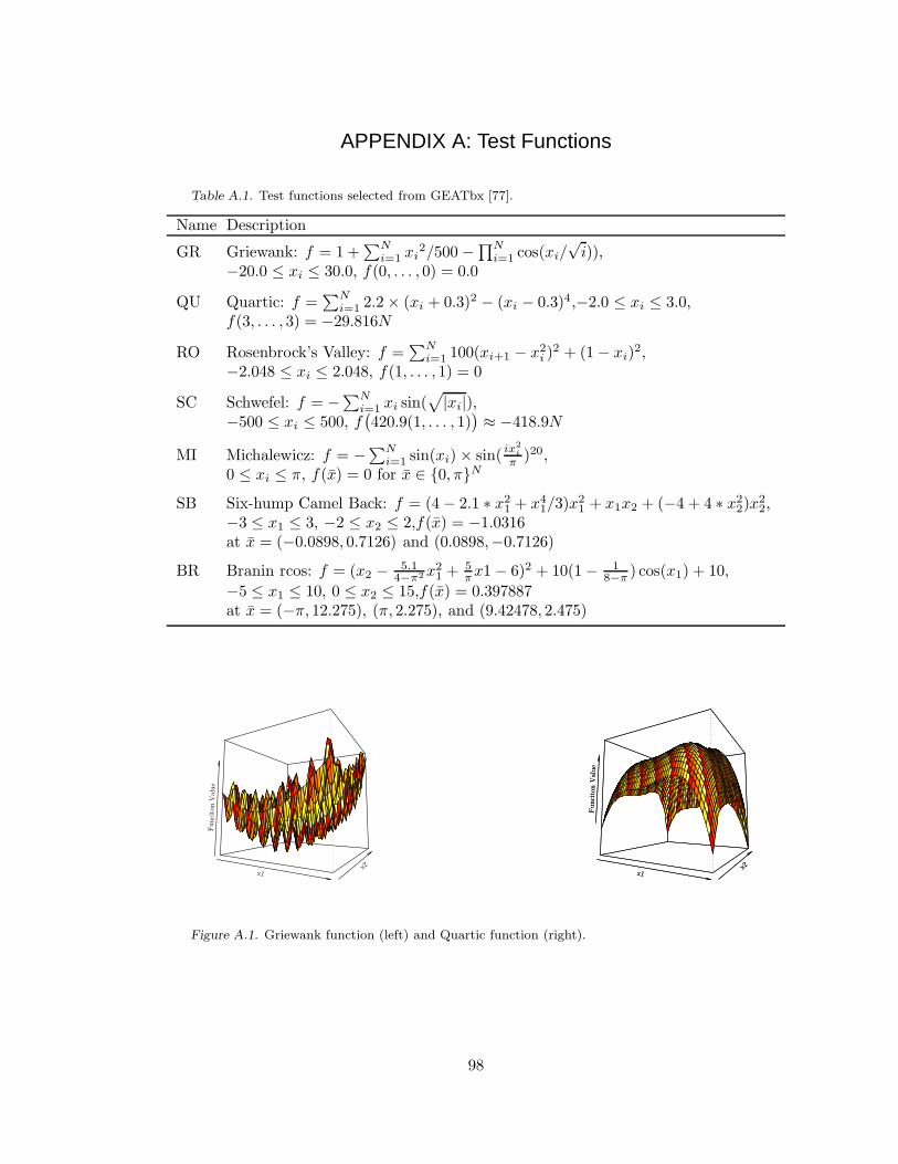
APPENDIX A: Test Functions
Table A.1. Test functions selected from GEATbx [77].
Name Description
GR Griewank: f = 1 +∑N
i=1 xi2/500 − ∏N
i=1 cos(xi/√
i)),−20.0 ≤ xi ≤ 30.0, f(0, . . . , 0) = 0.0
QU Quartic: f =∑N
i=1 2.2 × (xi + 0.3)2 − (xi − 0.3)4,−2.0 ≤ xi ≤ 3.0,f(3, . . . , 3) = −29.816N
RO Rosenbrock’s Valley: f =∑N
i=1 100(xi+1 − x2i )
2 + (1 − xi)2,
−2.048 ≤ xi ≤ 2.048, f(1, . . . , 1) = 0
SC Schwefel: f = −∑N
i=1 xi sin(√
|xi|),−500 ≤ xi ≤ 500, f
(
420.9(1, . . . , 1))
≈ −418.9N
MI Michalewicz: f = −∑N
i=1 sin(xi) × sin(ix2
i
π)20,
0 ≤ xi ≤ π, f(x) = 0 for x ∈ {0, π}N
SB Six-hump Camel Back: f = (4 − 2.1 ∗ x21 + x4
1/3)x21 + x1x2 + (−4 + 4 ∗ x2
2)x22,
−3 ≤ x1 ≤ 3, −2 ≤ x2 ≤ 2,f(x) = −1.0316at x = (−0.0898, 0.7126) and (0.0898,−0.7126)
BR Branin rcos: f = (x2 − 5.14−π2 x2
1 + 5πx1 − 6)2 + 10(1 − 1
8−π) cos(x1) + 10,
−5 ≤ x1 ≤ 10, 0 ≤ x2 ≤ 15,f(x) = 0.397887at x = (−π, 12.275), (π, 2.275), and (9.42478, 2.475)
x1x2
Funci
ton V
alue
x1x2
Funci
ton V
alue
x1x2
Funci
ton V
alue
Figure A.1. Griewank function (left) and Quartic function (right).
98

x1 x2
Funci
ton V
alue
x1x2
Funci
ton V
alue
Figure A.2. Rosenbrock’s Valley function (left) and Schwefel’s function (right).
x1x2
Funci
ton V
alue
x1x2
Funci
ton V
alue
Figure A.3. Michalewicz’s function (left) and Six-hump Camel Back function (right).
x1x2
Funci
ton V
alue
x1x2
Funci
ton V
alue
Figure A.4 . Branin rcos function.
99

APPENDIX B: VTDIRECT95
VTDIRECT95 is a Fortran 95 implementation of D.R. Jones’ deterministic global op-
timization algorithm DIRECT [56] introduced in Chapter 2. The package includes both a
serial code and a data-distributed massively parallel code for different problem scales and
optimization (exploration vs. exploitation) goals. As discussed in Chapter 3, dynamic data
structures are used to organize local data, handle unpredictable memory requirements, re-
duce the memory usage, and share the data across multiple processors. The parallel code
employs a multilevel functional and data parallelism (presented in Chapter 4) to boost
concurrency and mitigate the data dependency, thus improving the load balancing and
scalability. In addition, checkpointing features (described in Chapter 5) are integrated
into both versions to provide fault tolerance and hot restarts. The package organization,
portability, and usage are described in this chapter.
B.1. Package Organization
Figure B.1 shows the high level organization of VTDIRECT95. The module VTdirect MOD
declares the user called driver subroutine VTdirect for the serial code. Correspondingly,
the module pVTdirect MOD declares the user called parallel driver subroutine pVTdirect,
the subroutine pVTdirect init for MPI initialization, the subroutine pVTdirect finalize
for MPI finalization, as well as the data types, parameters, and auxiliary functions used
exclusively in the parallel code.
sample_pmain.f95
VTdirect.f95
VTdirect_MOD pVTdirect_MOD
pVTdirect.f95
sample_main.f95 objfunc.f95 use
include
module
file
REAL_PRECISION VTDIRECT_CHKPT
shared_modules.f95
VTDIRECT_COMMSUBVTDIRECT_GLOBAL
Figure B.1. The module/file dependency map.
The two driver subroutines VTdirect and pVTdirect share the modules: (1)
REAL PRECISION from HOMPACK90 ([94]) for specifying the real data type, (2) VTDI-
RECT GLOBAL containing definitions of derived data types, parameters, and module proce-
dures, (3) VTDIRECT COMMSUB containing the subroutines and functions common to both
the serial and parallel versions, and (4) VTDIRECT CHKPT defining data types and module
procedures for the checkpointing feature. These shared modules are merged in the file
shared modules.f95 as shown in Figure B.1. sample main and sample pmain are sam-
ple main programs that call VTdirect and pVTdirect, respectively, to optimize five test
100
objective functions defined in objfunc.f95 and verify the installation. The dependencies
between the package components are depicted in Figure B.1.
In the sample serial main program sample main each test objective function illustrates a
different way of calling the driver subroutine VTdirect. The calls illustrate the four different
stopping rules—maximum number of iterations MAX ITER, maximum number of function
evaluations MAX EVL, minimum box diameter MIN DIA, and minimum relative decrease in
objective function value OBJ CONV. For the last objective function, a multiple best box
(MBB) output is illustrated. Details of the arguments are in comments at the beginning of
the subroutine VTdirect. Different parallel schemes are used in the test cases for pVTdirect,
called by the sample parallel main program sample pmain. Both sample main programs
print to standard out the stopping rule satisfied, the minimum objective function value,
the minimum box diameter, and the number of iterations, function evaluations, and the
minimum vector(s). In addition, the test output for pVTdirect lists the number of masters
per subdomain and the number of subdomains.
Different computation precision and different compiled code on different systems may
require different numbers of iterations or evaluations to reach the desired solution accuracy
(1.0E-03) specified in the test programs. If a test program fails to locate the optimum value
or the optimum point given the stopping conditions in the supplied namelist input file, the
stopping conditions can be adjusted accordingly.
B.2. Portability Issues
The module REAL PRECISION from HOMPACK90 [94] is used to define real arithmetic
for “precision portability” across different systems. In the REAL PRECISION module, R8 is
the selected KIND value corresponding to real numbers with at least 13 decimal digits of
precision, covering 60-bit (Cray) and 64-bit (IEEE 754 Standard) real arithmetic.
Another portability issue arises under the parallel computing environment. Although
MPI is well known for its portability across machines, its latest standard has not proposed
a portable way of matching the data types specified with Fortran 95 KIND values. The
REAL (KIND=R8) real number may be considered as double precision on one system but as
single precision on another system. This data type matching problem is addressed here by
calling INQUIRE to obtain the byte size for the R8 type and using MPI BYTE to transfer a
buffer holding R8 values, assuming the same byte ordering on all the involved machines. No
performance degradation has been observed for this approach.
101
B.3. Usage Guide
One of the virtues of DIRECT, shared by VTDIRECT95, is that it only has one tuning
parameter (ǫ) beyond the problem definition and stopping condition. Using VTDIRECT95
basically takes three simple steps. First, define the objective function with an input argu-
ment for the point coordinates (c), an output argument for evaluation status (iflag), and
an output variable for the returned function value (f). A nonzero return value for iflag
is used to indicate that c is infeasible or f is undefined at c. The user written objective
function is a FUNCTION procedure that must conform to the interface:
INTERFACE
FUNCTION Obj Func(c, iflag) RESULT(f)
USE REAL PRECISION, ONLY: R8
REAL(KIND = R8), DIMENSION(:), INTENT(IN):: c
INTEGER, INTENT(OUT):: iflag
REAL(KIND = R8):: f
END FUNCTION Obj Func
END INTERFACE
Second, allocate the required arrays and specify appropriate input parameters to call
one of the driver subroutines. In the parallel case, the MPI initialization and finalization
subroutines need to be called before and after calling the parallel driver subroutine (pVTdi-
rect), unless MPI is initialized and finalized elsewhere in the same application. The required
arrays include the input lower (L) and upper (U) bounds, and an output array for the op-
timum vector (X). Additionally, in the parallel version, the return status is also an array,
required to be allocated beforehand, to hold statuses returned from subdomains, even if
only one domain exists, in which case the size of the status array is one. If the user desires
to specify the optional input argument BOX SET, an array of boxes must be allocated and
an optional weight array W for dimensional scaling may also be allocated.
All other input parameters specified in the argument list of the driver subroutine are
conveniently read in from a NAMELIST file, as illustrated in the sample main programs.
Using namelist files is an elegant way of varying input parameters as needed, without recom-
piling the program. The namelist file pdirectRO.nml shown below is to test pVTdirect for
optimizing the 4-dimensional problem RO. The parameters are grouped into four categories
(NAMELISTs): parallel scheme PSCHEME, problem configuration PROBLEM, optimization pa-
rameters OPTPARM, and checkpointing option CHKPTOP. This example uses two subdomains
and two masters per subdomain, and the stopping condition is when the minimum box
diameter reaches 1.0E-05. The checkpointing feature is activated when chkpt start equals
1 (saving) or 2 (recovery). The program will terminate if the checkpoint file errors occur
as explained in the section on error handling (Chapter 5). It is the user’s responsibility to
maintain the checkpoint files, including renaming or removing old files.
102

&PSCHEME n subdomains=2 n masters=2 bin=1 /
&PROBLEM N=4
LB(1:4)=-2.048,-2.048,-2.048,-2.048
UB(1:4)=2.048,2.048,2.048,2.048 /
&OPTPARM iter lim=0 eval lim=0 diam lim=1.0E-5 objf conv=0.0
eps fmin=0.0 c switch=1 min sep=0.0 weight(1:4)=1,1,1,1
n optbox=1 /
&CHKPTOP chkpt start=0 /
Finally, the last step is to interpret the return status, collect the results, and deallocate
the arrays as needed. The return status consists of two digits. The tens digit indicates
the general status: 0 for a successful run, 1 for an input parameter error, 2 for a memory
allocation error or failure, and 3 for a checkpoint file error. The stopping condition for a
successful run is further indicated in the units digit, which also points to the exact source
of error if a nonzero status is returned. For example, a return status of 33 means the
checkpoint file header does not match with the current setting. All the error codes and
interpretations can be found in the source code documentation. A successful run returns
the optimum value and vector(s) in the user-prepared variables and arrays. In order to
receive a report on the actual number of iterations/evaluations, or minimum box diameter,
these optional arguments must be present in the argument list. The final results of calling
pVTdirect are merged on processor 0 (the root master), so proc id is returned to designate
the root to report the results. VTDIRECT95 is designed so that the optimization results
may be directly fed to another procedure or process, the typical situation in large scale
scientific computing.
103
Appendix C: Shared Modules
The shared modules REAL PRECISION, VTDIRECT GLOBAL that defines data types,
parameters, and module procedures used by both VTdirect and pVTdirect, VTDI-
RECT COMMSUB that declares the subroutines and functions shared by VTdirect and pVTdi-
rect, and VTDIRECT CHKPT that defines data types and module procedules for the check-
pointing feature used in both VTdirect and pVTdirect are listed below.
MODULE REAL_PRECISION ! From HOMPACK90.
! This is for 64-bit arithmetic.
INTEGER, PARAMETER:: R8=SELECTED_REAL_KIND(13)
END MODULE REAL_PRECISION
MODULE VTDIRECT_GLOBAL
USE REAL_PRECISION
IMPLICIT NONE
!
!HyperBox: Defines an n-dimensional box.
! val - Function value at the box center.
! c - The center point coordinates.
! side - Box side lengths for all dimensions.
! diam - Box diameter squared.
!
TYPE HyperBox
REAL(KIND = R8) :: val
REAL(KIND = R8), DIMENSION(:), POINTER :: c
REAL(KIND = R8), DIMENSION(:), POINTER :: side
REAL(KIND = R8) :: diam
END TYPE HyperBox
!
!BoxLink: Contains 1-D array of hyperboxes, linked to each column of
! BoxMatrix when needed.
! Line - 1-D array of boxes.
! ind - Index of last box in array ’Line’.
! next - The pointer to the next BoxLink.
! prev - The pointer to the previous BoxLink.
!
TYPE BoxLink
TYPE(HyperBox), DIMENSION(:), POINTER :: Line
INTEGER :: ind
TYPE(BoxLink), POINTER :: next
TYPE(BoxLink), POINTER :: prev
END TYPE BoxLink
!
!P_BoxLink: Contains a pointer to a BoxLink for a column in BoxMatrix.
! p - Pointer to a BoxLink.
!
TYPE P_BoxLink
TYPE(BoxLink), POINTER :: p
END TYPE P_BoxLink
!
!BoxLine: Contains 1-D array of newly sampled hyperboxes.
! Line - 1-D array of boxes.
! ind - Index of last box in array ’Line’.
! dir - Directions in which box centers are sampled.
104

!
TYPE BoxLine
TYPE(HyperBox), DIMENSION(:), POINTER :: Line
INTEGER :: ind
INTEGER, DIMENSION(:), POINTER :: dir
END TYPE BoxLine
!
!BoxMatrix: Contains 2-D array of hyperboxes.
! M - 2-D array of boxes.
! ind - An array holding the number of boxes in all the columns in ’M’.
! child - The pointer to the next BoxMatrix with the smaller diameters.
! sibling - The pointer array for all columns, pointing to the next
! BoxLinks with the same diameters.
! id - Identifier of this box matrix among all box matrices.
!
TYPE BoxMatrix
TYPE(HyperBox), DIMENSION(:,:), POINTER :: M
INTEGER, DIMENSION(:), POINTER :: ind
TYPE(BoxMatrix), POINTER :: child
TYPE(P_BoxLink), DIMENSION(:), POINTER :: sibling
INTEGER :: id
END TYPE BoxMatrix
!
! P_Box: Contains a pointer to a hyperbox.
!
TYPE P_Box
TYPE (HyperBox), POINTER :: p_box
END TYPE P_Box
!
!int_vector : A list holding integer values.
! dim - The index of the last element in the list.
! elements - The integer array.
! flags - The integer array holding the status for ’elements’.
! Bit 0: status of convex hull processing.
! next - The pointer to the next integer vector list.
! prev - The pointer to the previous integer vector list.
! id - Identifier of this integer vector list among all lists.
!
TYPE int_vector
INTEGER :: dim
INTEGER, DIMENSION(:), POINTER :: elements
INTEGER, DIMENSION(:), POINTER :: flags
TYPE(int_vector), POINTER :: next
TYPE(int_vector), POINTER :: prev
INTEGER :: id
END TYPE int_vector
!
!real_vector: A list holding real values.
! dim - The index of the last element in the list.
! elements - The real array.
! next - The pointer to the next real vector list.
! prev - The pointer to the previous real vector list.
! id - Identifier of this real vector list among all lists.
!
TYPE real_vector
INTEGER :: dim
105
REAL(KIND = R8), DIMENSION(:), POINTER :: elements
TYPE(real_vector), POINTER :: next
TYPE(real_vector), POINTER :: prev
INTEGER :: id
END TYPE real_vector
!
!ValList: a list for sorting the wi for all dimensions i corresponding
! to the maximum side length. wi = min f(c+delta*ei), f(c-delta*ei),
! the minimum of objective function values at the center point c +
! delta*ei and the center point c - delta*ei, where delta is one-third of
! this maximum side length and ei is the ith standard basis vector.
! dim - The index of the last element in the list.
! val - An array holding the minimum function values.
! dir - An array holding the sampling directions corresponding to the
! function values in array ’val’.
!
TYPE ValList
INTEGER :: dim
REAL(KIND = R8), DIMENSION(:), POINTER :: val
INTEGER, DIMENSION(:), POINTER :: dir
END TYPE
! Parameters.
! Argument input error.
INTEGER, PARAMETER :: INPUT_ERROR = 10
! Allocation failure error.
INTEGER, PARAMETER :: ALLOC_ERROR = 20
! File I/O error.
INTEGER, PARAMETER :: FILE_ERROR = 30
! Stop rule 1: maximum iterations.
INTEGER, PARAMETER :: STOP_RULE1 = 0
! Stop rule 2: maximum evaluations.
INTEGER, PARAMETER :: STOP_RULE2 = 1
! Stop rule 3: minimum diameter.
INTEGER, PARAMETER :: STOP_RULE3 = 2
! Stop rule 4: minimum relative change in objective function.
INTEGER, PARAMETER :: STOP_RULE4 = 3
! ’flags’ bits for ’setInd’ of type ’int_vector’.
INTEGER, PARAMETER :: CONVEX_BIT = 0
! Bit 0: if set, the first box on the corresponding column is in the convex
! hull box set.
! Global variables.
INTEGER :: col_w, row_w ! Factors defining reasonable memory space for
! each box matrix allocation.
INTEGER :: N_I ! Local copy of ’N’.
REAL(KIND = R8) :: EPS4N
TYPE(Hyperbox), POINTER :: tempbox ! Box for swapping heap elements.
! Interfaces.
INTERFACE ASSIGNMENT (=)
MODULE PROCEDURE AssgBox
END INTERFACE
INTERFACE insNode
MODULE PROCEDURE insNodeI
MODULE PROCEDURE insNodeR
END INTERFACE insNode
INTERFACE rmNode
MODULE PROCEDURE rmNodeI
106
MODULE PROCEDURE rmNodeR
END INTERFACE rmNode
CONTAINS
SUBROUTINE AssgBox(x, y)
IMPLICIT NONE
! Copy the contents of box ’y’ to box ’x’.
!
! On input:
! y - Box with type ’HyperBox’.
!
! On output:
! x - Box with type ’HyperBox’ having contents of box ’y’.
!
TYPE(HyperBox), INTENT(IN) :: y
TYPE(HyperBox), INTENT(INOUT) :: x
x%val = y%val
x%diam = y%diam
x%c = y%c
x%side = y%side
RETURN
END SUBROUTINE AssgBox
SUBROUTINE insNodeR(n, pt, index, Set)
IMPLICIT NONE
! Insert a real number ’pt’ at the indexed position ’index’ of ’Set’.
!
! On input:
! n - The maximum length of the real array in each node of ’Set’.
! pt - The real number to be inserted to ’Set’.
! index - The position at which to insert ’pt’ in a node of ’Set’.
! Set - A linked list of type(real_vector) nodes.
!
! On output:
! Set - ’Set’ has an added real number and modified ’dim’ component.
!
INTEGER, INTENT(IN) :: n
REAL(KIND = R8), INTENT(IN) :: pt
INTEGER, INTENT(IN) :: index
TYPE(real_vector), INTENT(INOUT), TARGET :: Set
! Local variables.
TYPE(real_vector), POINTER :: p_set ! Pointer to a node of ’Set’.
! Insert ’pt’ into ’Set’.
IF (Set%dim < n ) THEN
! The head node is not full. There are no other nodes.
! Update ’dim’.
Set%dim = Set%dim + 1
IF (index == Set%dim) THEN
! The desired position is at end, so insert ’pt’ at end.
Set%elements(Set%dim) = pt
ELSE
! The desired position is not at end, so shift elements before
! insertion.
Set%elements(index+1:Set%dim) = Set%elements(index:Set%dim-1)
Set%elements(index) = pt
END IF
ELSE
! The head node is full. Check other nodes.
107

p_set => Set%next
! To shift elements, find the last node which is not full.
DO WHILE(p_set%dim == n)
p_set => p_set%next
END DO
! Found the last node ’p_set’ which is not full.
! Update ’dim’ of ’p_set’. Shift element(s) inside this node, if any.
p_set%dim = p_set%dim + 1
! Loop shifting until reaching the node ’Set’ at which to insert ’pt’.
DO WHILE(.NOT. ASSOCIATED(p_set, Set))
! Shift element(s) inside this node, if any.
p_set%elements(2:p_set%dim) = p_set%elements(1:p_set%dim-1)
! Shift the last element from the previous node to this one.
p_set%elements(1) = p_set%prev%elements(n)
! Finished shifting this node. Go to the previous node.
p_set => p_set%prev
END DO
! Reached the original node ’Set’.
IF (index == Set%dim) THEN
! The desired position is at end, so insert ’pt’ at end.
Set%elements(Set%dim) = pt
ELSE
! The desired position is not at end, so shift elements before
! insertion.
Set%elements(index+1:Set%dim) = Set%elements(index:Set%dim-1)
Set%elements(index) = pt
END IF
END IF
RETURN
END SUBROUTINE insNodeR
SUBROUTINE insNodeI(n, pt, index, Set)
IMPLICIT NONE
! Insert an integer number ’pt’ at the indexed position ’index’ of ’Set’.
!
! On input:
! n - The maximum length of the integer array in each node of ’Set’.
! pt - The integer number to be inserted to ’Set’.
! index - The position at which to insert ’pt’.
! Set - A linked list of type(int_vector) nodes.
!
! On output:
! Set - ’Set’ has an added integer number and modified ’dim’ component.
INTEGER, INTENT(IN) :: n
INTEGER, INTENT(IN) :: pt
INTEGER, INTENT(IN) :: index
TYPE(int_vector), INTENT(INOUT), TARGET :: Set
! Local variables.
TYPE(int_vector), POINTER :: p_set ! Pointer to a node of ’Set’.
LOGICAL :: setflags ! The flag to operate on component ’flags’.
! Assign ’setflags’.
setflags = ASSOCIATED(Set%flags)
! Insert ’pt’ into ’Set’.
IF (Set%dim < n ) THEN
! The head node is not full. There are no other nodes.
Set%dim = Set%dim + 1
IF (index == Set%dim) THEN
108

! The desired position is at end, so insert ’pt’ at end.
Set%elements(Set%dim) = pt
! Clear the ’flags’.
IF (setflags) Set%flags(Set%dim) = 0
ELSE
! The desired position is not at end, so shift elements before
! insertion.
Set%elements(index+1:Set%dim) = Set%elements(index:Set%dim-1)
IF (setflags) THEN
! Shift the ’flags’.
Set%flags(index+1:Set%dim) = Set%flags(index:Set%dim-1)
! Clear the ’flags’.
Set%flags(index) = 0
END IF
! Insert ’pt’.
Set%elements(index) = pt
END IF
ELSE
! The head node is full. There must be other nodes.
p_set => Set%next
! To shift elements, find the last node which is not full.
DO WHILE(p_set%dim == n)
p_set => p_set%next
END DO
! Found the last node ’p_set’ which is not full.
! Update ’dim’ of ’p_set’. Shift element(s), if any.
p_set%dim = p_set%dim + 1
! Loop shifting until reaching the original node ’Set’.
DO WHILE(.NOT. ASSOCIATED(p_set, Set))
! Shift element(s) inside this node, if any.
p_set%elements(2:p_set%dim) = p_set%elements(1:p_set%dim-1)
! Shift the last element from the previous node to this one.
p_set%elements(1) = p_set%prev%elements(n)
IF (setflags) THEN
! Shift the ’flags’.
p_set%flags(2:p_set%dim) = p_set%flags(1:p_set%dim-1)
p_set%flags(1) = p_set%prev%flags(n)
END IF
! Finished shifting this node. Go to the previous node.
p_set => p_set%prev
END DO
! Reached the original node ’Set’.
IF (index == Set%dim) THEN
! The desired position is at end, so insert ’pt’ at end.
Set%elements(Set%dim) = pt
! Clear the ’flags’.
IF (setflags) Set%flags(Set%dim) = 0
ELSE
! The desired position is not at end, so shift elements before
! insertion.
Set%elements(index+1:Set%dim) = Set%elements(index:Set%dim-1)
IF (setflags) THEN
! Shift the ’flags’.
Set%flags(index+1:Set%dim) = Set%flags(index:Set%dim-1)
! Clear the ’flags’.
Set%flags(index) = 0
109
END IF
! Insert ’pt’.
Set%elements(index) = pt
END IF
END IF
RETURN
END SUBROUTINE insNodeI
SUBROUTINE rmNodeI(n, offset, index, Set)
IMPLICIT NONE
! Remove an integer entry at position ’index’ from the integer array
! in the node at ’offset’ links from the beginning of the linked list
! ’Set’.
!
! On input:
! n - The maximum length of the integer array in each node of ’Set’.
! offset - The offset of the desired node from the first node of ’Set’.
! index - The position at which to delete an integer from the integer
! array in the node.
! Set - A linked list of type(int_vector) nodes.
!
! On output:
! Set - The desired node of ’Set’ has the indexed integer entry removed
! and the ’dim’ component modified.
!
INTEGER, INTENT(IN) :: n
INTEGER, INTENT(IN) :: offset
INTEGER, INTENT(IN) :: index
TYPE(int_vector), INTENT(INOUT), TARGET :: Set
! Local variables.
INTEGER :: i ! Loop counter.
TYPE(int_vector), POINTER :: p_set ! Pointer to a node of ’Set’.
LOGICAL :: setflags ! The flag to operate on component ’flags’.
! Assign ’setflags’.
setflags = ASSOCIATED(Set%flags)
! Find the desired node.
p_set => Set
DO i = 1, offset
p_set => p_set%next
END DO
IF (index < p_set%dim) THEN
! It’s not the last entry in ’p_set’, so shift elements.
p_set%elements(index:p_set%dim-1) = p_set%elements(index+1:p_set%dim)
! Shift the ’flags’.
IF (setflags) p_set%flags(index:p_set%dim-1) = p_set%flags(index+1:p_set%dim)
END IF
IF (p_set%dim < n) THEN
! There are not other elements in next node, so remove the indexed
! entry directly from ’Set’ by updating ’dim’.
p_set%dim = p_set%dim - 1
ELSE
! There might be nodes in which to shift elements.
! Check if any element(s) in next node to shift.
IF (ASSOCIATED(p_set%next)) THEN
p_set => p_set%next
DO
IF (p_set%dim > 0) THEN
110

! There are elements to shift.
! Shift one element from p_next into its previous node.
p_set%prev%elements(n) = p_set%elements(1)
! Shift elements inside p_next.
p_set%elements(1:p_set%dim-1) = p_set%elements(2:p_set%dim)
IF (setflags) THEN
! Shift the ’flags’.
p_set%prev%flags(n) = p_set%flags(1)
p_set%flags(1:p_set%dim-1) = p_set%flags(2:p_set%dim)
END IF
ELSE
! There are no elements to shift. Update ’dim’ of previous node.
p_set%prev%dim = p_set%prev%dim - 1
EXIT
END IF
! Move on to the next node, if any. If there are no more nodes, update
! ’dim’.
IF (ASSOCIATED(p_set%next)) THEN
p_set => p_set%next
ELSE
p_set%dim = p_set%dim - 1
EXIT
END IF
END DO
ELSE
! There are no more nodes. Update ’dim’ of ’p_set’.
p_set%dim = p_set%dim - 1
END IF
END IF
RETURN
END SUBROUTINE rmNodeI
SUBROUTINE rmNodeR(n, offset, index, Set)
IMPLICIT NONE
! Remove a real entry at position ’index’ from the real array
! in the node at ’offset’ links from the beginning of the linked list
! ’Set’.
!
! On input:
! n - The maximum length of the real array in each node of ’Set’.
! offset - The offset of the desired node from the first node of ’Set’.
! index - The position at which to delete a real entry from the real
! array in the node.
! Set - A linked list of type(real_vector) nodes.
!
! On output:
! Set - The desired node of ’Set’ has the indexed real entry removed
! and the ’dim’ component modified.
!
INTEGER, INTENT(IN) :: n
INTEGER, INTENT(IN) :: offset
INTEGER, INTENT(IN) :: index
TYPE(real_vector), INTENT(INOUT), TARGET :: Set
! Local variables.
INTEGER :: i ! Loop counter.
TYPE(real_vector), POINTER :: p_set ! Pointer to a node of ’Set’.
! Find the desired node.
111
p_set => Set
DO i = 1, offset
p_set => p_set%next
END DO
IF (index < p_set%dim)THEN
! It’s not the last entry in ’p_set’, so shift elements.
p_set%elements(index:p_set%dim-1) = p_set%elements(index+1:p_set%dim)
END IF
IF (p_set%dim < n) THEN
! There are not other elements in next node, so remove the indexed
! entry directly from ’Set’ by updating ’dim’.
p_set%dim = p_set%dim - 1
ELSE
! There might be nodes in which to shift elements.
! Check if any element(s) in next node to shift.
IF (ASSOCIATED(p_set%next)) THEN
p_set => p_set%next
DO
IF (p_set%dim > 0) THEN
! There are elements to shift.
! Shift one element from p_next into its previous node.
p_set%prev%elements(n) = p_set%elements(1)
! Shift elements inside p_next.
p_set%elements(1:p_set%dim-1) = p_set%elements(2:p_set%dim)
ELSE
! There are no elements to shift. Update ’dim’ of previous node.
p_set%prev%dim = p_set%prev%dim - 1
EXIT
END IF
! Move on to the next node if any. If there are no more nodes, update
! ’dim’.
IF (ASSOCIATED(p_set%next)) THEN
p_set => p_set%next
ELSE
p_set%dim = p_set%dim - 1
EXIT
END IF
END DO
ELSE
! There are no more nodes. Update ’dim’ of ’p_set’.
p_set%dim = p_set%dim - 1
END IF
END IF
RETURN
END SUBROUTINE rmNodeR
END MODULE VTDIRECT_GLOBAL
MODULE VTDIRECT_COMMSUB
USE VTDIRECT_GLOBAL
INTERFACE OPERATOR (.lexLT.) ! Lexicographic comparison operator.
MODULE PROCEDURE lexOrder
END INTERFACE
CONTAINS
SUBROUTINE binaryS(p_rset, diam, pos, found)
IMPLICIT NONE
! Using a binary search, match the squared diameter ’diam’ with an
! element in the node ’p_rset’ of ’setDia’, and return the position
112
! ’pos’ if a match is found. If there is no match, return the right
! ’pos’ at which to insert ’diam’. When ’pos’ is returned as 0, ’diam’
! should be inserted after all others. If ’pos’ is not 0, ’diam’ could
! be inserted at the position ’pos’ of ’p_rset’ depending on ’found’.
! See insMat().
! On input:
! p_rset - A pointer to one of the nodes in ’setDia’.
! diam - The diameter squared to match against.
!
! On output:
! pos - The position in ’p_rset’ for a match or insertion.
! found - Status indicating whether ’diam’ is found in ’p_rest’ or not.
!
TYPE(real_vector), INTENT(IN) :: p_rset
REAL(KIND = R8), INTENT(IN) :: diam
INTEGER, INTENT(OUT) :: pos
LOGICAL, INTENT(OUT) :: found
! Local variables.
INTEGER :: low, mid, up
! Initialization for searching.
found = .FALSE.
! Initialize limits outside bounds of array for binary search.
low = 0
up = p_rset%dim + 1
IF (p_rset%dim > 0) THEN
! Check with the first and the last.
IF (p_rset%elements(1) <= diam) THEN
! ’diam’ is the biggest.
IF (ABS(p_rset%elements(1) - diam)/MAX(diam, p_rset%elements(1)) <= EPS4N) THEN
! ’diam’ is the same as the first one.
found = .TRUE.
END IF
pos = 1
RETURN
ELSE
IF (p_rset%elements(up-1) >= diam) THEN
IF (ABS(p_rset%elements(up-1) - diam)/MAX(p_rset%elements(up-1), diam) &
<= EPS4N) THEN
! ’diam’ is the smallest one. Same as the last one in ’p_rset’.
found = .TRUE.
pos = up-1
ELSE
! ’diam’ is smaller than all in ’p_rset’. Set ’pos’ 0 to insert
! ’diam’ after all others.
found = .FALSE.
pos = 0
END IF
RETURN
ELSE
! ’diam’ falls in between the biggest and the smallest. Apply binary
! search.
DO WHILE((low + 1) < up)
mid = (low + up) / 2
IF (ABS(diam - p_rset%elements(mid))/ &
MAX(diam, p_rset%elements(mid)) <= EPS4N) THEN
! ’diam’ found.
113

up = mid
EXIT
END IF
IF (diam < p_rset%elements(mid))THEN
low = mid
ELSE
up = mid
END IF
END DO
! Check if it’s found.
mid = up
IF (ABS(diam - p_rset%elements(mid))/MAX(diam, p_rset%elements(mid)) &
<= EPS4N) THEN
! Found it, so assign ’mid’ to ’pos’ in order to insert the
! associated box in the same column as ’mid’.
found = .TRUE.
pos = mid
ELSE
found = .FALSE.
IF (diam > p_rset%elements(mid) )THEN
! ’diam’ is bigger than the one at ’mid’. Set ’pos’ to be ’mid’
! in order to insert ’diam’ before ’mid’.
pos = mid
ELSE
! ’diam’ is smaller than the one at ’mid’. Set ’pos’ to be one
! after ’mid’ in order to insert ’diam’ after ’mid’.
pos = mid + 1
END IF
END IF
END IF
END IF
ELSE
! ’p_rset’ is empty. Set ’pos’=0 to insert ’diam’ at the end of ’p_rset’.
found = .FALSE.
pos = 0
END IF
RETURN
END SUBROUTINE binaryS
SUBROUTINE checkblinks(col, b, status)
IMPLICIT NONE
! Check if this column needs a new box link. Create one if needed.
!
! On input:
! col - The local column index.
! b - The current link of box matrices.
!
! On output:
! b - ’b’ has the newly added box link for ’col’ if needed.
! status - Return status.
! 0 Successful.
! 1 Allocation error.
!
INTEGER, INTENT(IN) :: col
TYPE(BoxMatrix), INTENT(INOUT) :: b
INTEGER, INTENT(OUT) :: status
! Local variables.
114
TYPE(BoxLink), POINTER :: newBoxLink, p_link
INTEGER :: i
! Set normal status.
status = 0
IF ((b%ind(col) == row_w) .AND. (.NOT. ASSOCIATED(b%sibling(col)%p))) THEN
! When the M part of the box column is full and there are no box links:
! Make a new box link linked to it. Allocate a new one.
ALLOCATE(newBoxLink, STAT = status)
IF (status /= 0) RETURN
CALL initLink(newBoxLink, status)
IF (status /= 0) RETURN
! This is the first box link that does not have previous link.
NULLIFY(newBoxLink%prev)
! Link it as ’sibling’ of this column.
b%sibling(col)%p => newBoxLink
ELSE ! There is at least one box link.
IF (b%ind(col) > row_w) THEN
! Find the last box link ’p_blink’.
p_link => b%sibling(col)%p
DO i=1,(b%ind(col)-1)/row_w-1
p_link => p_link%next
END DO
IF ((p_link%ind == row_w) .AND. (.NOT. ASSOCIATED(p_link%next))) THEN
! It’s full.
! Need a new box link. Allocate a new one.
ALLOCATE(newBoxLink, STAT = status)
IF (status /= 0) RETURN
CALL initLink(newBoxLink, status)
IF (status /= 0) RETURN
! Link the new box link to the last one as the next link.
p_link%next => newBoxLink
! Link the last box link to the new one as the previous link.
newBoxLink%prev => p_link
END IF
END IF
END IF
RETURN
END SUBROUTINE checkblinks
FUNCTION findpt(b, col, i_last, index, p_last) RESULT(p_index)
IMPLICIT NONE
! Find the pointer for the box ’index’ in the column ’col’ of box
! matrix ’b’. If this box ’index’ is in one of the box links, record
! the pointer to the box link holding this box ’index’ in ’p_last’
! and compute the box position offset ’i_last’. These two records will
! be used to resume chasing the pointers for the heap elements closer
! to the bottom.
!
! On input:
! b - Box matrix holding the box column ’col’ with the box ’index’.
! col - Column index.
! i_last - Box position offset used in finding the starting box position
! from the box link ’p_last’.
! index - Box index.
! p_last - Pointer to the last box link that has been chased so far.
!
! On output:
115

! i_last - Updated ’i_last’.
! p_last - Updated ’p_last’.
!
TYPE(BoxMatrix), INTENT(IN), TARGET :: b
INTEGER, INTENT(IN) :: col
INTEGER, INTENT(INOUT) :: i_last
INTEGER, INTENT(IN) :: index
TYPE(BoxLink), POINTER :: p_last
TYPE(HyperBox), POINTER :: p_index
! Local variables.
TYPE(BoxLink), POINTER :: p_l ! Pointer to a box link.
INTEGER :: i
IF (.NOT. ASSOCIATED(p_last)) THEN
! ’p_last’ has not been set, so start from the first box matrix ’b’.
IF (index <= row_w) THEN
! The box ’index’ is in ’M’ array of ’b’.
p_index => b%M(index,col)
ELSE
! Chase to the box link that this box belongs to.
p_l => b%sibling(col)%p
DO i = 1, (index-1)/row_w -1
p_l => p_l%next
END DO
! Found the box link that holds the box ’index’.
p_index => p_l%Line(MOD(index-1, row_w)+1)
! Set ’p_last’ and ’i_last’.
p_last => p_l
i_last = ((index-1)/row_w)*row_w
END IF
ELSE
! Start from ’p_last’, because it is the last box link that has been
! processed.
p_l => p_last
DO i = 1, (index-i_last-1)/row_w
p_l => p_l%next
END DO
! Found the box link that holds the box ’index’.
p_index => p_l%Line(MOD(index-1,row_w)+1)
! Set ’p_last’ and ’i_last’.
p_last => p_l
i_last = ((index-1)/row_w)*row_w
END IF
RETURN
END FUNCTION findpt
SUBROUTINE initLink(newBoxLink, iflag)
IMPLICIT NONE
! Initialize a new box link.
!
! On input:
! newBoxLink - A new box link.
!
! On output:
! newBoxLink - ’newBoxLink’ with initialized structures.
! iflag - Return status.
! 0 Normal.
! 1 Allocation failure.
116
!
TYPE(BoxLink), INTENT(INOUT) :: newBoxLink
INTEGER, INTENT(OUT) :: iflag
! Local variables.
INTEGER :: i
! Initialize ’iflag’.
iflag = 0
! Allocate ’Line’ of the new BoxLink.
ALLOCATE(newBoxLink%Line(row_w),STAT = iflag)
IF (iflag /= 0) RETURN
DO i = 1, row_w
ALLOCATE(newBoxLink%Line(i)%c(N_I),STAT = iflag)
IF (iflag /= 0) RETURN
ALLOCATE(newBoxLink%Line(i)%side(N_I),STAT = iflag)
IF (iflag /= 0) RETURN
END DO
! Nullify pointers ’next’ and ’prev’.
NULLIFY(newBoxLink%next)
NULLIFY(newBoxLink%prev)
! Initialize the counter for boxes.
newBoxLink%ind = 0
RETURN
END SUBROUTINE initLink
SUBROUTINE insBox(box, col, b, iflag)
IMPLICIT NONE
! Insert ’box’ in column ’col’ of box matrices ’b’. If all positions
! in ’col’ are full, make a new box link linked to the end of
! this column.
!
! On input:
! box - The box to be inserted.
! col - The global column index at which to insert ’box’.
! b - The head link of box matrices.
!
! On output:
! b - ’b’ has a newly added ’box’.
! iflag - Return status.
! 0 Normal.
! 1 Allocation failure.
!
TYPE(HyperBox), INTENT(IN) :: box
INTEGER, INTENT(IN) :: col
TYPE(BoxMatrix), INTENT(INOUT), TARGET :: b
INTEGER, INTENT(OUT) :: iflag
! Local variables.
INTEGER :: b_id, i, mycol, status
TYPE(BoxLink), POINTER :: p_blink
TYPE(BoxMatrix), POINTER :: p_b
! Initialize ’iflag’ as a normal return.
iflag = 0
! Locate the box matrix in which to insert ’box’.
mycol = col
IF (mycol <= col_w) THEN
p_b => b
ELSE
b_id = (mycol-1)/col_w + 1
117

mycol = MOD(mycol-1, col_w) + 1
p_b => b
DO i=1, b_id-1
p_b => p_b%child
END DO
END IF
! Insert the box at the end of column ’mycol’ of box matrix ’p_b’.
IF (p_b%ind(mycol) < row_w) THEN
! There is no box links.
p_b%M(p_b%ind(mycol)+1, mycol) = box
ELSE
! There are box links. Chase to the last box link.
p_blink => p_b%sibling(mycol)%p
DO i = 1, p_b%ind(mycol)/row_w - 1
p_blink => p_blink%next
END DO
p_blink%ind = p_blink%ind + 1
p_blink%Line(p_blink%ind) = box
END IF
! Update ’ind’ of the column (’ind’ of ’p_b’ counts all the boxes in
! this column including the ones in its box links.).
p_b%ind(mycol) = p_b%ind(mycol) + 1
! Siftup the box in the heap.
CALL siftup(p_b, mycol, p_b%ind(mycol))
! Add a new box link if needed.
CALL checkblinks(mycol, p_b, status)
IF (status /=0) THEN ; iflag = 1 ; END IF
RETURN
END SUBROUTINE insBox
SUBROUTINE insMat(box, b, setDia, setInd, setFcol, status, isConvex)
IMPLICIT NONE
! Retrieve all box matrices to find the place at which to insert ’box’.
! Insert it in the column with the same squared diameter, or a new
! column if the squared diameter is new. In the same column, the smaller
! ’val’, the earlier the position.
!
! On input:
! box - The box to be inserted.
! b - The head link of box matrices.
! setDia - A linked list holding different squared diameters.
! setInd - A linked list holding the column indices corresponding to
! ’setDia’.
! setFcol - A linked list holding free columns of box matrices.
! isConvex- A flag to indicate if ’box’ is on the convex hull.
!
! On output:
! b - ’b’ has the newly added ’box’ and updated counters.
! setDia - ’setDia’ has a newly added squared diameter if any and
! updated ’dim’ if modified.
! setInd - ’setInd’ has a newly added column index if needed and
! updated ’dim’ if modified.
! setFcol - ’setFcol’ has a column index removed if needed and updated
! ’dim’ if modified.
! status - Status of processing.
! 0 Normal.
! 1 Allocation failures of type ’BoxMatrix’.
118
! 2 Allocation failures of type ’BoxLink’.
! 3 Allocation failures of type ’real_vector’ or ’int_vector’.
!
!
TYPE(HyperBox), INTENT(IN) :: box
TYPE(BoxMatrix), INTENT(INOUT), TARGET :: b
TYPE(real_vector), INTENT(INOUT), TARGET :: setDia
TYPE(int_vector), INTENT(INOUT), TARGET :: setInd
TYPE(int_vector), INTENT(INOUT), TARGET :: setFcol
INTEGER, INTENT(OUT) :: status
INTEGER, INTENT(IN) :: isConvex
! Local variables.
INTEGER :: b_id, b_pos, i, iflag, j, pos
LOGICAL :: found
TYPE(BoxMatrix), POINTER :: p_b
TYPE(int_vector), POINTER :: p_iset
TYPE(real_vector), POINTER :: p_rset
! Initialization for msearchSet().
pos = 0
found = .FALSE.
NULLIFY(p_rset)
iflag = 0
status = 0
! Locate a node of ’setDia’ into which ’diam’ can be inserted.
p_rset => msearchSet(setDia, box%diam)
CALL binaryS(p_rset, box%diam, pos, found)
IF (found) THEN
! A match is found in ’p_rset’ of ’setDia’.
! Find the corresponding node in ’setInd’ to match ’p_rset’.
p_iset => setInd
DO i = 1, p_rset%id-1
p_iset => p_iset%next
END DO
! Insert ’box’ in the column indexed by ’pos’ in a node of ’setInd’.
CALL insBox(box, p_iset%elements(pos), b, iflag)
IF (iflag == 1 ) THEN ; status = 2 ; RETURN ; END IF
IF (isConvex == 1) THEN ! Set ’CONVEX_BIT’.
p_iset%flags(pos) = IBSET(p_iset%flags(pos), CONVEX_BIT)
END IF
ELSE
! No match is found. It’s a new squared diameter.
IF (pos == 0)THEN
! Obtain a free column from ’setFcol’ to insert ’box’ after all
! other columns.
IF (setFcol%dim > 0)THEN
! ’setFcol’ is not empty, so pop a column from the top of ’setFcol’
! nodes.
IF (setFcol%dim < col_w) THEN
! The head node is not full, therefore it must be the top node.
i = setFcol%elements(setFcol%dim)
! Update ’dim’.
setFcol%dim = setFcol%dim - 1
ELSE
! There might be other nodes with element(s).
p_iset => setFcol%next
IF (ASSOCIATED(p_iset)) THEN
119
! Chase to the top node of ’setFcol’ with element(s).
DO WHILE(p_iset%dim == col_w)
p_iset => p_iset%next
END DO
! The top node could be ’p_iset’ or its ’prev’.
IF (p_iset%dim /= 0) THEN
i = p_iset%elements(p_iset%dim)
p_iset%dim = p_iset%dim - 1
ELSE
i = p_iset%prev%elements(p_iset%prev%dim)
p_iset%prev%dim = p_iset%prev%dim - 1
END IF
ELSE
! There are no more nodes with elements. Pop a column from the
! head node of ’setFcol’.
i = setFcol%elements(setFcol%dim)
! Update ’dim’.
setFcol%dim = setFcol%dim -1
END IF
END IF
ELSE
! There are no free columns, so make a new box matrix.
CALL newMat(b, setDia, setInd, setFcol, iflag)
IF (iflag /= 0) THEN ; status = iflag ; RETURN ; END IF
! Pop a column from the top of ’setFcol’ for use.
i = setFcol%elements(setFcol%dim)
CALL rmNode(col_w, 0, setFcol%dim, setFcol)
END IF
! Found the global column index ’i’ at which to insert ’box’. Convert
! it to a local column index ’b_pos’ and locate the box
! matrix ’p_b’ at which to insert ’box’.
IF (i <= col_w) THEN
p_b => b
b_pos = i
ELSE
b_id = (i-1)/col_w + 1
b_pos = MOD(i-1, col_w) + 1
p_b => b
DO j = 1, b_id -1
p_b => p_b%child
END DO
END IF
! Insert ’box’ at the beginning of the new column ’b_pos’.
p_b%M(1,b_pos) = box
! Locate the nodes in both ’setDia’ and ’setInd’ at which to insert
! the new squared diameter and the column index ’i’ at the end of
! both linked lists (’pos’ is 0).
IF (setDia%dim < col_w)THEN
! There are no more nodes with elements. Assign the head node
! to ’p_rset’.
p_rset => setDia
ELSE
! There are other nodes to check.
p_rset => setDia%next
IF (ASSOCIATED(p_rset)) THEN
! Chase to the end of the linked list.
120
DO WHILE(p_rset%dim == col_w)
p_rset => p_rset%next
END DO
ELSE
! There are no more nodes. Assign the head node to ’p_rset’
p_rset => setDia
END IF
END IF
! Found the node ’p_rset’ of ’setDia’ to insert.
CALL insNode(col_w, box%diam, p_rset%dim+1, p_rset)
! Find the corresponding node in ’setInd’ at which to insert the
! column index ’i’.
p_iset => setInd
DO j =1, p_rset%id -1
p_iset => p_iset%next
END DO
CALL insNode(col_w, i, p_iset%dim+1, p_iset)
! Set ’CONVEX_BIT’.
IF (isConvex == 1) p_iset%flags(p_iset%dim) = &
IBSET(p_iset%flags(p_iset%dim), CONVEX_BIT)
! Update ’ind’ of col ’b_pos’ in ’p_b’.
p_b%ind(b_pos) = 1
ELSE
! ’pos’ is not 0. ’p_rset’ points to the right node of ’setDia’ to
! insert the new squared diameter.
! Obtain a free column from ’setFcol’ to insert a new column before the
! column indexed by the returned ’pos’.
IF (setFcol%dim > 0)THEN
! ’setFcol’ is not empty, so pop a column from the top of ’setFcol’
! nodes.
IF (setFcol%dim < col_w) THEN
! The head node is not full, so it must be the top.
i = setFcol%elements(setFcol%dim)
setFcol%dim = setFcol%dim - 1
ELSE
! There might be nodes with free columns.
p_iset => setFcol%next
IF (ASSOCIATED(p_iset)) THEN
! Chase to the top of ’setFcol’ links.
DO WHILE(p_iset%dim == col_w)
p_iset => p_iset%next
END DO
! The top node could be ’p_iset’ or its ’prev’.
IF (p_iset%dim /= 0) THEN
i = p_iset%elements(p_iset%dim)
p_iset%dim = p_iset%dim - 1
ELSE
i = p_iset%prev%elements(p_iset%prev%dim)
p_iset%prev%dim = p_iset%prev%dim - 1
END IF
ELSE
! There are no more nodes with elements. Pop a column from the
! head node of ’setFcol’.
i = setFcol%elements(setFcol%dim)
setFcol%dim = setFcol%dim -1
END IF
121

END IF
ELSE
! There are no free columns, so make a new box matrix.
CALL newMat(b, setDia, setInd, setFcol, iflag)
IF (iflag /= 0) THEN ; status = iflag ; RETURN ; END IF
! Pop a column for use.
i = setFcol%elements(setFcol%dim)
CALL rmNode(col_w, 0, setFcol%dim, setFcol)
END IF
! Found the global column index ’i’ at which to insert ’box’.
! Convert it to a local column index ’b_pos’ and locate the
! box matrix ’p_b’ in which to insert ’box’.
IF (i <= col_w) THEN
p_b => b
b_pos = i
ELSE
b_id = (i-1)/col_w + 1
b_pos = MOD(i-1, col_w) + 1
p_b => b
DO j = 1, b_id -1
p_b => p_b%child
END DO
END IF
! Add ’box’ to be the first on column ’b_pos’ of ’p_b’.
p_b%M(1,b_pos) = box
! Insert the new squared diameter at the position ’pos’ in ’p_rset’
! of ’setDia’.
CALL insNode(col_w, box%diam, pos, p_rset)
! Insert the corresponding column index ’i’ at the same position ’pos’
! in a node of ’setInd’.
p_iset => setInd
DO j = 1, p_rset%id -1
p_iset => p_iset%next
END DO
CALL insNode(col_w, i, pos, p_iset)
IF (isConvex == 1) p_iset%flags(pos) = &
IBSET(p_iset%flags(pos), CONVEX_BIT)
! Update ’ind’ of box matrix ’p_b’.
p_b%ind(b_pos) = 1
END IF
END IF
RETURN
END SUBROUTINE insMat
FUNCTION lexOrder(a, b) RESULT (smaller)
IMPLICIT NONE
! Compare box centers ’a’ and ’b’ lexicographically. If ’a’ is
! lexicographically smaller than ’b’, return .TRUE. . Define operator
! .lexLT. .
!
! On input:
! a - center of a box.
! b - center of a box.
!
! On output:
! smaller - .TRUE. ’a’ is smaller than ’b’ lexicographically.
! .FALSE. Otherwise.
122
!
REAL(KIND = R8), DIMENSION(:), INTENT(IN) :: a
REAL(KIND = R8), DIMENSION(:), INTENT(IN) :: b
LOGICAL :: smaller
! Local variables.
INTEGER :: i
! Initialize ’smaller’.
smaller = .FALSE.
! Loop for comparing coordinates of ’a’ and ’b’.
DO i = 1,SIZE(a)
IF (a(i) < b(i)) THEN
smaller = .TRUE.
EXIT
ELSE IF (a(i) == b(i)) THEN
CONTINUE
ELSE ! a(i) > b(i)
EXIT
END IF
END DO
RETURN
END FUNCTION lexOrder
FUNCTION msearchSet(setDia, diam) RESULT(p_rset)
IMPLICIT NONE
! Find the right node in ’setDia’ in which to insert ’diam’.
!
! On input:
! setDia - A linked list holding different squared diameters.
! diam - A diameter squared to be inserted in a node in ’setDia’.
!
! On output:
! p_rset - Pointer to the right node of ’setDia’.
!
TYPE(real_vector), INTENT(IN), TARGET :: setDia
REAL(KIND = R8), INTENT(IN) :: diam
TYPE(real_vector), POINTER :: p_rset
! Local variables.
TYPE(real_vector), POINTER :: p_setDia
! Initialize ’p_setDia’.
p_setDia => setDia
DO
IF (p_setDia%dim > 0) THEN
! There are elements to be compared with ’diam’.
IF (diam >= p_setDia%elements(1)) THEN
! ’diam’ is the biggest. Return this node as ’p_rset’.
p_rset => p_setDia
EXIT
ELSE
IF ((diam >= p_setDia%elements(p_setDia%dim)) .OR. &
((ABS(diam - p_setDia%elements(p_setDia%dim)) &
/MAX(diam, p_setDia%elements(p_setDia%dim))) <= EPS4N) ) THEN
! ’diam’ is within the range of elements in this node.
p_rset => p_setDia
EXIT
ELSE
! ’diam’ is smaller than the last element. Go on to the next
! node, if any.
123

IF (ASSOCIATED(p_setDia%next)) THEN
p_setDia => p_setDia%next
ELSE
! There are no more nodes. Return this pointer.
p_rset => p_setDia
EXIT
END IF
END IF
END IF
ELSE
! It’s empty. Return this pointer.
p_rset => p_setDia
EXIT
END IF
END DO
RETURN
END FUNCTION msearchSet
SUBROUTINE newMat(b, setDia, setInd, setFcol, iflag)
IMPLICIT NONE
! Make a new box matrix and its associated linked lists for holding
! different squared diameters, column indices, and free columns.
! Link them to existing structures.
!
! On input:
! b - The head link of box matrices.
! setDia - Linked list holding different squared diameters of
! current boxes.
! setInd - Linked list holding column indices of box matrices.
! setFcol - Linked list holding free columns of box matrices.
!
! On output:
! b - ’b’ has a box matrix link added at the end.
! setDia - ’setDia’ has a node added at the end.
! setInd - ’setInd’ has a node added at the end.
! setFcol - ’setFcol’ has a node added at the end.
! iflag - Return status.
! 0 Normal.
! 1 Allocation failures of type ’BoxMatrix’.
! 3 Allocation failures of type ’real_vector’ or ’int_vector’.
!
TYPE(BoxMatrix), INTENT(INOUT), TARGET :: b
TYPE(real_vector), INTENT(INOUT), TARGET :: setDia
TYPE(int_vector), INTENT(INOUT), TARGET :: setInd
TYPE(int_vector), INTENT(INOUT), TARGET :: setFcol
INTEGER, INTENT(OUT) :: iflag
! Local variables.
INTEGER :: alloc_err, i, j
TYPE(BoxMatrix), POINTER :: new_b, p_b
TYPE(int_vector), POINTER :: n_setFcol, n_setInd, p_setFcol, p_setInd
TYPE(real_vector), POINTER :: n_setDia, p_setDia
! Initialize iflag for normal return.
iflag = 0
! Allocate a new box matrix.
ALLOCATE(new_b, STAT=alloc_err)
IF (alloc_err /= 0) THEN; iflag = 1; RETURN; END IF
! Allocate its associated arrays.
124

ALLOCATE(new_b%M(row_w, col_w), STAT=alloc_err)
IF (alloc_err /= 0) THEN; iflag = 1; RETURN; END IF
ALLOCATE(new_b%ind(col_w), STAT=alloc_err)
IF (alloc_err /= 0) THEN; iflag = 1; RETURN; END IF
! Clear the box counter for each column.
new_b%ind(:) = 0
! Nullify pointers for a child link and box links.
NULLIFY(new_b%child)
ALLOCATE(new_b%sibling(col_w), STAT=alloc_err)
IF (alloc_err /= 0) THEN; iflag = 1; RETURN; END IF
DO i = 1, col_w
NULLIFY(new_b%sibling(i)%p)
END DO
DO i = 1, row_w
DO j = 1, col_w
ALLOCATE(new_b%M(i,j)%c(N_I), STAT=alloc_err)
IF (alloc_err /= 0) THEN; iflag = 1; RETURN; END IF
ALLOCATE(new_b%M(i,j)%side(N_I), STAT=alloc_err)
IF (alloc_err /= 0) THEN; iflag = 1; RETURN; END IF
END DO
END DO
! Find the last box matrix to link with the new one.
p_b => b
DO WHILE(ASSOCIATED(p_b%child))
p_b => p_b%child
END DO
! Found the last box matrix p_b. Link it to new box matrix ’b’.
p_b%child => new_b
! Set up ’id’ for new_b.
new_b%id = p_b%id + 1
! Allocate new ’setDia’, ’setInd’ and ’setFcol’ for ’new_b’.
! Find the corresponding nodes of ’setDia’, ’setInd’ and ’setFcol’.
p_setDia => setDia
p_setInd => setInd
p_setFcol => setFcol
DO i=1, p_b%id-1
p_setDia => p_setDia%next
p_setInd => p_setInd%next
p_setFcol => p_setFcol%next
END DO
! Allocate a new node for ’setDia’. Initialize its structure.
ALLOCATE(n_setDia, STAT=alloc_err)
IF (alloc_err /= 0) THEN; iflag = 3; RETURN; END IF
ALLOCATE(n_setDia%elements(col_w), STAT=alloc_err)
IF (alloc_err /= 0) THEN; iflag = 3; RETURN; END IF
NULLIFY(n_setDia%next)
NULLIFY(n_setDia%prev)
n_setDia%id = p_setDia%id +1
n_setDia%dim = 0
! Allocate a new node for ’setInd’. Initialize its structure.
ALLOCATE(n_setInd, STAT=alloc_err)
IF (alloc_err /= 0) THEN; iflag = 3; RETURN; END IF
ALLOCATE(n_setInd%elements(col_w), STAT=alloc_err)
IF (alloc_err /= 0) THEN; iflag = 3; RETURN; END IF
ALLOCATE(n_setInd%flags(col_w), STAT=alloc_err)
IF (alloc_err /= 0) THEN; iflag = 3; RETURN; END IF
125
n_setInd%flags(:)= 0
NULLIFY(n_setInd%next)
NULLIFY(n_setInd%prev)
n_setInd%id = p_setInd%id + 1
n_setInd%dim = 0
! Allocate a new node for ’setFcol’. Initialize its structure.
ALLOCATE(n_setFcol, STAT=alloc_err)
IF (alloc_err /= 0) THEN; iflag = 3; RETURN; END IF
ALLOCATE(n_setFcol%elements(col_w), STAT=alloc_err)
IF (alloc_err /= 0) THEN; iflag = 3; RETURN; END IF
NULLIFY(n_setFcol%next)
NULLIFY(n_setFcol%prev)
n_setFcol%id = p_setFcol%id + 1
n_setFcol%dim = 0
! Link them to the end of existing sets.
p_setDia%next => n_setDia
n_setDia%prev => p_setDia
p_setInd%next => n_setInd
n_setInd%prev => p_setInd
p_setFcol%next => n_setFcol
n_setFcol%prev => p_setFcol
! Fill up ’setFcol’ with new columns from the new box matrix.
! Starting from the last column, push free columns to the top of ’setFcol’.
DO i = 1, col_w
setFcol%elements(i) = new_b%id*col_w - (i-1)
END DO
setFcol%dim = col_w
RETURN
END SUBROUTINE newMat
SUBROUTINE siftdown(b, col, index)
IMPLICIT NONE
! Sift down the heap element at ’index’ through the heap column ’col’ in
! the box matrix ’b’.
!
! On input:
! b - Box matrix holding the box column ’col’ for siftdown.
! col - Column index.
! index - Index of the box to be sifted down.
!
! On output:
! b - Box matrix with the elements rearranged by siftdown.
!
TYPE(BoxMatrix), INTENT(INOUT), TARGET :: b
INTEGER, INTENT(IN) :: col, index
! Local variables.
INTEGER :: i ! Loop counters.
INTEGER :: i_last ! Index of the last box that has been processed
! in the previous iteration.
INTEGER :: i_last_backup ! i_last’s backup used to go back to i_last,
! which may be updated in the current iteration.
INTEGER :: left, right ! Indices for the left and right children.
TYPE(BoxLink), POINTER :: p_last ! Pointer to the last box link
! that has been processed.
TYPE(BoxLink), POINTER :: p_last_backup ! Pointer backup for ’p_last’.
TYPE(HyperBox), POINTER :: p_i ! Pointer to the heap parent box.
TYPE(HyperBox), POINTER :: p_left, p_right ! Pointers to the left and right
126
! child boxes.
! Exit if it is an empty column.
IF (b%ind(col) == 0) RETURN
! Initialization.
NULLIFY(p_last)
i_last=0
! Starting siftdown operation from the box ’index’
i = index
DO
! Find the indices for the left and right children.
left = 2*i
right = 2*i + 1
! If ’i’ is a leaf, exit.
IF (left > b%ind(col)) EXIT
! Find the pointers to the the ith box and its left child. Record the
! pointer ’p_last’ and index ’i_last’ for the currently processed box
! link.
p_i => findpt(b, col, i_last, i, p_last)
p_left => findpt(b, col, i_last, left, p_last)
IF (left < b%ind(col)) THEN
! Backup the pointer ’p_last’ and the index ’i_last’, because they will
! be updated when finding the pointer to the right child. If the right
! child is in the correct place in the heap, restore the pointer
! ’p_last’ and the index ’i_last’.
p_last_backup => p_last
i_last_backup = i_last
p_right => findpt(b, col, i_last, right, p_last)
IF (p_left%val > p_right%val) THEN
p_left => p_right
left = left + 1
ELSE
IF (p_left%val == p_right%val) THEN
! When values are equal, smaller lex order wins.
IF (p_right%c .lexLT. p_left%c) THEN
p_left => p_right
left = left + 1
ELSE
! Restore ’p_last’ and ’i_last’ to the values before finding
! the pointer for the right child.
p_last => p_last_backup
i_last = i_last_backup
END IF
ELSE
! Restore ’p_last’ and ’i_last’ to the values before finding
! the pointer for the right child.
p_last => p_last_backup
i_last = i_last_backup
END IF
END IF
END IF
! If the boxes are in the correct order, exit.
IF (p_i%val < p_left%val) EXIT
IF ((p_i%val == p_left%val) .AND. (p_i%c .lexLT. p_left%c)) EXIT
! Swap the boxes pointed to by ’pi’ and ’p_left’.
tempbox = p_i
p_i = p_left
127
p_left = tempbox
! Continue siftdown operation from the left child of ’i’.
i = left
END DO
RETURN
END SUBROUTINE siftdown
SUBROUTINE siftup(b, col, index)
IMPLICIT NONE
! Sift up the heap element at ’index’ through the heap column ’col’ in
! the box matrix ’b’.
!
! On input:
! b - Box matrix holding the box column ’col’ for siftup.
! col - Column index.
! index - Index of the box to be sifted up.
!
! On output:
! b - Box matrix with the elements rearranged by siftup.
!
TYPE(BoxMatrix), INTENT(INOUT), TARGET :: b
INTEGER, INTENT(IN) :: col, index
! Local variables.
INTEGER :: i, j ! Loop counters.
INTEGER :: parent ! Index for the parent.
INTEGER :: e_idi, e_idp, l_idi, l_idp
TYPE(BoxLink), POINTER :: p_blinki, p_blinkp ! Pointers for the box link.
TYPE(HyperBox), POINTER :: p_i ! Pointer to the box indexed as ’i’.
TYPE(HyperBox), POINTER :: p_p ! Pointer to the parent box.
! Exit if it is an empty column.
IF (b%ind(col) == 0) RETURN
! Starting siftup operation from the box ’index’.
i = index
IF (i == 1) RETURN ! Exit if there is only one box in the column.
l_idi = (i-1)/row_w ! If 0, it’s inside the box matrix M.
e_idi = MOD(i-1,row_w)+1
! Locate the box ’i’.
IF (l_idi == 0) THEN
p_i => b%M(i, col)
ELSE
! Chase to the box link that this box belongs to.
p_blinki => b%sibling(col)%p
DO j = 1, l_idi-1
p_blinki => p_blinki%next
END DO
! Found the box link that holds the box ’i’.
p_i => p_blinki%Line(e_idi)
END IF
DO WHILE (i /= 1) ! If the root has been reached, exit.
! Find the index for the parent.
parent = i/2
! Compute link id and element id for the parent.
l_idp = (parent-1)/row_w
e_idp = MOD(parent-1,row_w)+1
! Locate the box ’parent’.
IF (l_idp == 0) THEN
p_p => b%M(parent, col)
128

ELSE
p_blinkp => b%sibling(col)%p
DO j = 1, l_idp-1
p_blinkp => p_blinkp%next
END DO
p_p => p_blinkp%Line(e_idp)
END IF
! Found the boxes ’parent’ and ’i’. Compare their ’val’s. If box ’i’ has
! a smaller ’val’, swap box ’i’ with box ’parent’. Otherwise, box ’i’
! moves up to point to the box ’parent’ and repeats the comparison and
! swaps (if needed), until box ’i’ becomes the root.
IF ((p_i%val < p_p%val) .OR. &
((p_i%val == p_p%val) .AND. (p_i%c .lexLT. p_p%c))) THEN
tempbox = p_i
p_i = p_p
p_p = tempbox
l_idi = l_idp
e_idi = e_idp
i = parent
p_i => p_p
IF (l_idi /= 0) p_blinki => p_blinkp
ELSE
i = 1
END IF
END DO
RETURN
END SUBROUTINE siftup
END MODULE VTDIRECT_COMMSUB
MODULE VTDIRECT_CHKPT
USE VTDIRECT_GLOBAL
USE VTDIRECT_COMMSUB
!
! Definitions of derived data types.
!
! LogNode: Defines a checkpoint log node that contains a box’s center
! coordinates and the objective function value there.
! c - Point coordinates.
! val - The function value at ’c’.
!
TYPE LogNode
REAL(KIND = R8), DIMENSION(:), POINTER :: c
REAL(KIND = R8) :: val
END TYPE LogNode
!
! LogList: Contains a list of checkpoint logs. These logs are listed in
! the order that they were written to the checkpoint file when recovering
! in the case of the sequential run of VTdirect or the parallel run of
! pVTdirect with the same number of masters that generated the checkpoint
! logs. When the number of masters is different from that in the run that
! generated the checkpoint logs, these logs in the list are sorted in
! lexicographical order to facilitate a binary search to look up the function
! values.
! idx - Index to a log node during recovery, index of last log node
! during construction. idx is initialized to 0; if the logs are
! all recovered and the list is deallocated, idx is set to -1.
! list - List of log nodes.
129

!
TYPE LogList
INTEGER :: idx
TYPE(LogNode), DIMENSION(:), POINTER :: list
END TYPE LogList
!
! Definitions of global parameters, and variables.
!
INTEGER, PARAMETER :: CHKSUNIT=444 ! Logical unit number for a checkpoint
! file, or a base logical unit number for a set of checkpoint files when
! multiple files are kept open to recover the checkpoint logs from
! multiple masters in the parallel code pVTdirect. To avoid conflicts
! with other logical units in the same application, this value should
! be adjusted accordingly.
INTEGER, PARAMETER :: CHKRUNIT=CHKSUNIT+1 ! The second base logical unit
! number is needed for writing to a set of new checkpoint files when
! restarting with a number of masters different from that in the run that
! generated the checkpoint file (only in pVTdirect).
INTEGER, PARAMETER :: INITLEN = 1000 ! The initial length of the log list.
TYPE(LogList) :: fList ! The list of checkpoint logs.
CONTAINS
!
! Internal subroutines and functions.
!
RECURSIVE FUNCTION bFindlex(c, s, e) RESULT (ans)
IMPLICIT NONE
! Do a recursive binary search for ’c’ starting at position ’s’ and ending at
! position ’e’ in the log list sorted in lexicographical order.
!
! On input:
! c - Point coordinates.
! s - Starting position.
! e - Ending position.
!
! On output:
! ans - The position that c matches. If 0, ’c’ is not found.
!
REAL(KIND = R8), DIMENSION(:), INTENT(IN) :: c
INTEGER, INTENT(IN) :: s, e
INTEGER :: ans
! Local variables.
INTEGER :: mid ! The middle position.
! When ’s’ and ’e’ meet, check if ’c’ is found.
IF (s == e) THEN
IF (ALL(c == fList%list(s)%c)) THEN
ans = s
ELSE ! ’c’ is not found in the list.
ans = 0
END IF
ELSE
! Compute ’mid’ to recursively search the list in two divided portions.
mid = CEILING((s+e)*0.5_R8)
IF (c .lexLT. fList%list(mid)%c) THEN
ans = bFindlex(c, s, mid-1)
ELSE
ans = bFindlex(c, mid, e)
130
END IF
END IF
RETURN
END FUNCTION bFindlex
SUBROUTINE cleanList()
IMPLICIT NONE
! Deallocate the list structure of logs to release the memory and set a flag.
!
! On input: None.
!
! On output: None.
!
! Local variable.
INTEGER :: i
! Deallocate all log nodes in the list.
DO i = 1, SIZE(fList%list)
DEALLOCATE(fList%list(i)%c)
END DO
DEALLOCATE(fList%list)
! Set a flag that the log list has been deallocated.
fList%idx = -1
RETURN
END SUBROUTINE cleanList
SUBROUTINE enlargeList(len, copy)
IMPLICIT NONE
! Enlarge the current log list to size ’len’. The stored logs are
! preserved when ’copy’ is .TRUE..
!
! On input:
! len - The larger size of the list.
! copy - A switch indicating whether to copy the original content in
! the list. If .TRUE., the original logs will be copied to a
! temporary buffer and then stored at the beginning of the
! enlarged list.
!
! On output:
! fList%list - A larger list.
!
INTEGER, INTENT(IN) :: len
LOGICAL, INTENT(IN) :: copy
! Local variables.
INTEGER :: i
TYPE(LogNode), DIMENSION(:), ALLOCATABLE :: tmplist
! Exit if ’len’ is not larger.
IF (len <= SIZE(fList%list)) RETURN
! Allocate ’tmplist’ to temporarily store original logs.
IF (copy) THEN
ALLOCATE(tmplist(fList%idx))
DO i = 1, fList%idx
ALLOCATE(tmplist(i)%c(N_I))
tmplist(i)%c = fList%list(i)%c
tmplist(i)%val = fList%list(i)%val
END DO
END IF
! Deallocate the current list.
CALL cleanList()
131

! Reallocate the list with size ’len’.
CALL initList(len)
! Copy back the original list and deallocate the log nodes in ’tmplist’.
IF (copy) THEN
DO i = 1, SIZE(tmplist)
fList%list(i)%c = tmplist(i)%c
fList%list(i)%val = tmplist(i)%val
fList%idx = fList%idx + 1
DEALLOCATE(tmplist(i)%c)
END DO
! Deallocate ’tmplist’.
DEALLOCATE(tmplist)
END IF
RETURN
END SUBROUTINE enlargeList
FUNCTION idxList() RESULT (ans)
IMPLICIT NONE
! Return the used size ’idx’ of the list.
!
! On input: None.
!
! On output:
! ans - ’idx’ of ’fList’.
!
INTEGER :: ans
ans = fList%idx
RETURN
END FUNCTION idxList
FUNCTION inList(c, val) RESULT(ans)
IMPLICIT NONE
! Recover the function value ’val’ at ’c’ in the order it was recorded
! at the list. ’inList’ is called by VTdirect, and by pVTdirect only when
! the number of masters for the recovery run is the same as that for
! the run that generated the checkpoint file.
!
! On input:
! c - Point coordinates.
!
! On output:
! val - The function value at ’c’.
! ans - .TRUE. if ’val’ is found.
! .FALSE. if ’c’ is not matched.
!
REAL(KIND = R8), DIMENSION(:), INTENT(IN) :: c
REAL(KIND = R8), INTENT(OUT) :: val
LOGICAL :: ans
! Initialize ’ans’.
ans = .FALSE.
! Update the index to the newest recovered log.
fList%idx = fList%idx + 1
! Exit when idx is out of range.
IF ((fList%idx > SIZE(fList%list)).OR.(fList%idx < 1)) RETURN
IF (ALL(c == fList%list(fList%idx)%c)) THEN
! Found ’c’ and return ’val’.
val = fList%list(fList%idx)%val
ans = .TRUE.
132

ELSE
END IF
RETURN
END FUNCTION inList
SUBROUTINE initList(len)
IMPLICIT NONE
! Initialize the list of checkpoint logs.
!
! On input:
! len - The number of log nodes to be initialized.
!
! On output:
! fList%list - Initialized list.
!
INTEGER, INTENT(IN) :: len
! Local variable.
INTEGER :: i
! Allocate ’fList’ and ’len’ number of log nodes.
ALLOCATE(fList%list(len))
DO i = 1, len
ALLOCATE(fList%list(i)%c(N_I))
END DO
! Initialize ’idx’.
fList%idx = 0
RETURN
END SUBROUTINE initList
SUBROUTINE insList(c, val)
IMPLICIT NONE
! Insert ’c’ and ’val’ to the log list and update the index.
!
! On input:
! c - Point coordinates.
! val - The function value at ’c’.
!
! On output:
! fList%list - The updated log list.
!
REAL(KIND = R8), DIMENSION(:), INTENT(IN) :: c
REAL(KIND = R8), INTENT(IN) :: val
! Enlarge the list to be twice the current size if needed.
IF (fList%idx + 1 > SIZE(fList%list)) THEN
CALL enlargeList(2*SIZE(fList%list), .TRUE.)
END IF
! Increase ’idx’.
fList%idx = fList%idx + 1
! Add ’c’ and ’val’.
fList%list(fList%idx)%c = c
fList%list(fList%idx)%val = val
RETURN
END SUBROUTINE insList
FUNCTION lookupTab(c, val) RESULT(ans)
IMPLICIT NONE
! Do a binary search for ’c’ to retrieve the corresponding function value
! ’val’ in the table of logs sorted in lexicographical order.
! ’lookupTab’ is only called by pVTdirect when the number of masters in
! the recovery run has changed from that in the run that generated the
133
! checkpoint logs.
!
! On input:
! c - Point coordinates.
!
! On output:
! val - The function value at ’c’.
! ans - .TRUE. if ’c’ is found.
! .FALSE. if ’c’ is not found.
!
REAL(KIND = R8), DIMENSION(:), INTENT(IN) :: c
REAL(KIND = R8), INTENT(OUT) :: val
LOGICAL :: ans
! Local variables.
INTEGER :: i
! Initialize ’ans’.
ans = .FALSE.
! Do a binary search for ’c’ in the table of logs sorted lexicographically.
i = bFindlex(c, 1, fList%idx)
IF (i /= 0) THEN
! ’c’ is found, return ’val’.
val = fList%list(i)%val
ans = .TRUE.
END IF
RETURN
END FUNCTION lookupTab
FUNCTION moreList() RESULT (ans)
IMPLICIT NONE
! Return the recovery status of the log list ’fList’.
!
! On input: None.
!
! On output:
! ans - .TRUE. if the list has more logs to recover.
! .FALSE. if the list has no more logs to recover.
!
LOGICAL :: ans
! Initialize ’ans’.
ans = .TRUE.
IF (fList%idx == -1) ans = .FALSE.
RETURN
END FUNCTION moreList
SUBROUTINE resetList()
IMPLICIT NONE
! Reset the index of the function value list to 0, preparing for
! recovery.
!
! On input: None.
!
! On output: Reset index in the function value list.
!
fList%idx = 0
RETURN
END SUBROUTINE resetList
SUBROUTINE siftdownList(pos, len)
IMPLICIT NONE
134
! Sift down the log at position ’pos’ in the list with ’len’ logs.
!
! On input:
! pos - Position of the log to be sifted down.
! len - The length of the list.
!
! On output:
! fList%list - A log list with the log at position ’pos’ sifted down.
!
INTEGER, INTENT(IN) :: pos, len
! Local variables.
INTEGER :: i, left
IF (len == 0) RETURN ! Exit if there are no logs in the list.
i = pos ! Let ’i’ start at the log at ’pos’.
DO
left = 2*i ! Find the ’left’ child of the log at ’i’.
IF (left > len) EXIT ! Exit when log ’i’ is a leaf.
! Find the larger one of the left and right (left+1) children.
IF (left+1 <= len) THEN
! Let ’left’ point to the right child (if present) if it is larger.
IF (fList%list(left)%c .lexLT. fList%list(left+1)%c) left = left + 1
END IF
! Compare ’left’ child with the parent ’i’. Exit when ’i’ is larger.
IF (fList%list(left)%c .lexLT. fList%list(i)%c) EXIT
! Because ’i’ is smaller, swap logs at ’i’ and ’left’.
CALL swapList(i, left)
i = left ! Move down ’i’.
END DO
RETURN
END SUBROUTINE siftdownList
FUNCTION sizeList() RESULT (ans)
IMPLICIT NONE
! Return the size of the list.
!
! On input: None.
!
! On output:
! ans - Size of the log list ’fList’.
!
INTEGER :: ans
ans = SIZE(fList%list)
RETURN
END FUNCTION sizeList
SUBROUTINE sortList()
IMPLICIT NONE
! Sort the logs in the list.
!
! On input: None.
!
! On output:
! fList - Sorted list of checkpoint logs.
!
! Local variables.
INTEGER :: i
! Heapify the entire list to be a maxheap.
DO i = fList%idx/2, 1, -1
135

CALL siftdownList(i, fList%idx)
END DO
! Sort the list in ascending lexicographical order.
DO i=1, fList%idx
! Swap the largest one at the beginning with the one at end of the list.
CALL swapList(1, fList%idx-(i-1))
! Sift down the first one.
CALL siftdownList(1, fList%idx-i)
END DO
RETURN
END SUBROUTINE sortList
SUBROUTINE swapList(i, j)
IMPLICIT NONE
! Swap logs at positions ’i’ and ’j’ in the list.
!
! On input:
! i - Position of the first log to be swapped.
! j - Position of the second log to be swapped.
!
! On output:
! fList%list - Log list with positions ’i’ and ’j’ swapped.
!
INTEGER, INTENT(IN) :: i, j
! Local variables.
REAL(KIND = R8), DIMENSION(N_I) :: tmpc
REAL(KIND = R8) :: tmpf
IF (i == j) RETURN ! Exit when ’i’ equals ’j’.
! Copy log ’i’ to temporary variables.
tmpc = fList%list(i)%c
tmpf = fList%list(i)%val
! Copy log ’j’ to ’i’.
fList%list(i)%c = fList%list(j)%c
fList%list(i)%val = fList%list(j)%val
! Copy back log ’i’ to log ’j’
fList%list(j)%c = tmpc
fList%list(j)%val = tmpf
RETURN
END SUBROUTINE swapList
END MODULE VTDIRECT_CHKPT
136
Appendix D: Comments for VTdirect MOD
The comments for the module VTdirect MOD that declares subroutines and functions
used in the serial VTDIRECT implementation are listed from the source code as below.
MODULE VTdirect_MOD
USE VTDIRECT_GLOBAL ! Module (shared_modules.f95) for data types,
! parameters, global variables, interfaces, and internal subroutines.
USE VTDIRECT_COMMSUB ! Module (shared_modules.f95) for subroutines
! commonly used by VTdirect and pVTdirect.
USE VTDIRECT_CHKPT ! Module (shared_modules.f95) for data types,
! subroutines, functions, global variables used by checkpointing.
CONTAINS
SUBROUTINE VTdirect(N, L, U, OBJ_FUNC, X, FMIN, STATUS, SWITCH, &
MAX_ITER, MAX_EVL, MIN_DIA, OBJ_CONV, EPS, &
MIN_SEP, W, BOX_SET, NUM_BOX, RESTART)
IMPLICIT NONE
! This is a serial implementation of the DIRECT global unconstrained
! optimization algorithm described in:
!
! D.R. Jones, C.D. Perttunen, and B.E. Stuckman, Lipschitzian
! optimization without the Lipschitz constant, Journal of Optimization
! Theory and Applications, Vol. 79, No. 1, 1993, pp. 157-181.
!
! The algorithm to minimize f(x) inside the box L <= x <= U is as follows:
!
! 1. Normalize the search space to be the unit hypercube. Let c_1 be
! the center point of this hypercube and evaluate f(c_1).
! 2. Identify the set S of potentially optimal rectangles.
! 3. For all rectangles j in S:
! 3a. Identify the set I of dimensions with the maximum side length.
! Let delta equal one-third of this maximum side length.
! 3b. Sample the function at the points c +- delta*e_i for all i
! in I, where c is the center of the rectangle and e_i is the
! ith unit vector.
! 3c. Divide the rectangle containing c into thirds along the
! dimensions in I, starting with the dimension with the lowest
! value of f(c +- delta*e_i) and continuing to the dimension
! with the highest f(c +- delta*e_i).
! 4. Repeat 2.-3. until stopping criterion is met.
!
! On input:
!
! N is the dimension of L, U, and X.
!
! L(1:N) is a real array giving lower bounds on X.
!
! U(1:N) is a real array giving upper bounds on X.
!
! OBJ_FUNC is the name of the real function procedure defining the
! objective function f(x) to be minimized. OBJ_FUNC(C,IFLAG) returns
! the value f(C) with IFLAG=0, or IFLAG/=0 if f(C) is not defined.
! OBJ_FUNC is precisely defined in the INTERFACE block below.
!
! Optional arguments:
137
!
! SWITCH =
! 1 select potentially optimal boxes on the convex hull of the
! (box diameter, function value) points (default).
! 0 select as potentially optimal the box with the smallest function
! value for each diameter that is above the roundoff level.
! This is an aggressive selection procedure that generates many more
! boxes to subdivide.
!
! MAX_ITER is the maximum number of iterations (repetitions of Steps 2-3)
! allowed; defines stopping rule 1. If MAX_ITER is present but <= 0
! on input, there is no iteration limit and the number of iterations
! executed is returned in MAX_ITER.
!
! MAX_EVL is the maximum number of function evaluations allowed; defines
! stopping rule 2. If MAX_EVL is present but <= 0 on input, there is no
! limit on the number of function evaluations, which is returned in
! MAX_EVL.
!
! MIN_DIA is the minimum box diameter allowed; defines stopping rule 3.
! If MIN_DIA is present but <= 0 on input, a minimum diameter below
! the roundoff level is not permitted, and the box diameter of the
! box containing the smallest function value FMIN is returned in
! MIN_DIA.
!
! OBJ_CONV is the smallest acceptable relative improvement in the minimum
! objective function value ’FMIN’ between iterations; defines
! stopping rule 4. OBJ_CONV must be positive and greater than the round
! off level. If absent, it is taken as zero.
!
! EPS is the tolerance defining the minimum acceptable potential
! improvement in a potentially optimal box. Larger EPS values
! eliminate more boxes from consideration as potentially optimal,
! and bias the search toward exploration. EPS must be positive and
! greater than the roundoff level. If absent, it is taken as
! zero. EPS > 0 is incompatible with SWITCH = 0.
!
! MIN_SEP is the specified minimal (weighted) distance between the
! center points of the boxes returned in the optional array BOX_SET.
! If absent or invalid, MIN_SEP is taken as 1/2 the (weighted) diameter
! of the box [L, U].
!
! W(1:N) is a positive real array. The distance between two points X
! and Y is defined as SQRT(SUM( (X-Y)*W*(X-Y) )). If absent, W is
! taken as all ones.
!
! BOX_SET is an empty array (TYPE HyperBox) allocated to hold the desired
! number of boxes.
!
! RESTART =
! 0, checkpointing is off (default).
! 1, all function evaluations are logged to a file.
! 2, the program restarts from the checkpoint file ’vtdirchkpt.dat’
! and new function evaluation logs will be appended to the end of
! the file.
!
138

! On output:
!
! X(1:N) is a real vector containing the sampled box center with the
! minimum objective function value FMIN.
!
! FMIN is the minimum function value.
!
! STATUS is a return status flag. The units decimal digit specifies
! which stopping rule was satisfied on a successful return. The tens
! decimal digit indicates a successful return, or an error condition
! with the cause of the error condition reported in the units digit.
!
! Tens digit =
! 0 Normal return.
! Units digit =
! 1 Stopping rule 1 (iteration limit) satisfied.
! 2 Stopping rule 2 (function evaluation limit) satisfied.
! 3 Stopping rule 3 (minimum diameter reached) satisfied. The
! minimum diameter corresponds to the box for which X and
! FMIN are returned.
! 4 Stopping rule 4 (relative change in ’FMIN’) satisfied.
! 1 Input data error.
! Units digit =
! 0 N < 2.
! 1 Assumed shape array L, U, W, or X does not have size N.
! 2 Some lower bound is >= the corresponding upper bound.
! 3 MIN_DIA, OBJ_CONV, or EPS is invalid or below the roundoff level.
! 4 None of MAX_EVL, MAX_ITER, MIN_DIA, and OBJ_CONV are specified;
! there is no stopping rule.
! 5 Invalid SWITCH value.
! 6 SWITCH = 0 and EPS > 0 are incompatible.
! 7 RESTART has an invalid value.
! 2 Memory allocation error or failure.
! Units digit =
! 0 BoxMatrix type allocation.
! 1 BoxLink or BoxLine type allocation.
! 2 int_vector or real_vector type allocation.
! 3 HyperBox type allocation.
! 4 BOX_SET is allocated with a wrong problem dimension.
! 3 Checkpoint file error.
! Units digit =
! 0 Open error. If RESTART==1, an old checkpoint file vtdirchkpt.dat
! may be present and needs to be removed. If RESTART==2,
! vtdirchkpt.dat does not exist.
! 1 Read error.
! 2 Write error.
! 3 The file header does not match with the current setting.
! 4 A log is missing in the file for recovery.
!
! Optional arguments:
!
! MAX_ITER (if present) contains the number of iterations.
!
! MAX_EVL (if present) contains the number of function evaluations.
!
! MIN_DIA (if present) contains the diameter of the box associated with
139

! X and FMIN.
!
! MIN_SEP (if present) is unchanged if it was a reasonable value on
! input. Otherwise, it is reset to the default value.
!
! W (if present) is unchanged if it was positive on input. Any
! non-positive component is reset to one.
!
! BOX_SET (if present) is an array of TYPE (HyperBox) containing the
! best boxes with centers separated by at least MIN_SEP.
! The number of returned boxes NUM_BOX <= SIZE(BOX_SET) is as
! large as possible given the requested separation.
!
! NUM_BOX (if present) is the number of boxes returned in the array
! BOX_SET(1:).
!
140
Appendix E: Comments for pVTdirect MOD
The comments for the module pVTdirect MOD that defines data types, subroutines,
and functions used in the parallel VTDIRECT implementation are listed from the source
code as below.
MODULE pVTdirect_MOD
USE VTDIRECT_GLOBAL ! Module (shared_modules.f95) for data types,
! parameters, global variables, interfaces, and internal subroutines.
USE VTDIRECT_COMMSUB ! Module (shared_modules.f95) for subroutines
! used by VTdirect and pVTdirect in common.
USE VTDIRECT_CHKPT ! Module (shared_modules.f95) for data types,
! subroutines, functions, global variables used by checkpointing.
INCLUDE "mpif.h" ! MPI library functions.
!
!OptResults: Contains the search results for a subdomain.
! fmin - Minimum function value.
! x - The point coordinates associated with ’fmin’.
! max_iter - Number of iterations.
! max_evl - Number of evaluations.
! min_dia - Minimum diameter.
! status - Search return status.
!
TYPE OptResults
REAL(KIND = R8) :: fmin
REAL(KIND = R8), DIMENSION(:), POINTER :: x
INTEGER :: max_iter
INTEGER :: max_evl
REAL(KIND = R8) :: min_dia
INTEGER :: status
END TYPE OptResults
! MPI message types.
! A nonblocking function evaluation request.
INTEGER, PARAMETER :: NONBLOCK_REQ = 1
! A blocking function evaluation request.
INTEGER, PARAMETER :: BLOCK_REQ = 2
! Point(s) responding to a nonblocking request.
INTEGER, PARAMETER :: POINT_NBREQ = 3
! Point(s) responding to a blocking request.
INTEGER, PARAMETER :: POINT_BREQ = 4
! No more point for evaluation.
INTEGER, PARAMETER :: NO_POINT = 5
! Returned point function value(s).
INTEGER, PARAMETER :: FUNCVAL = 6
! All search work is done.
INTEGER, PARAMETER :: MYALL_DONE = 7
! Updating the global counter for the blocked workers.
INTEGER, PARAMETER :: COUNT_DONE = 8
! Search results.
INTEGER, PARAMETER :: RESULT_DATA = 9
! Converting a master to a worker.
INTEGER, PARAMETER :: BE_WORKER = 11
! Termination.
INTEGER, PARAMETER :: TERMINATE = 13
! Updating intermediate search results.
141
INTEGER, PARAMETER :: UPDATES = 14
! MPI error.
INTEGER, PARAMETER :: DMPI_ERROR = 40
CONTAINS
SUBROUTINE pVTdirect_finalize()
! MPI finalization.
!
! On input: None.
!
! On output: None.
!
! Local variable.
INTEGER :: ierr
CALL MPI_FINALIZE(ierr)
RETURN
END SUBROUTINE pVTdirect_finalize
SUBROUTINE pVTdirect_init(iflag)
! MPI initialization.
!
! On input: None.
!
! On output:
! iflag - Initialization status.
!
INTEGER, INTENT(OUT) :: iflag
iflag = 0
CALL MPI_INIT(iflag)
IF (iflag /= MPI_SUCCESS) THEN
iflag = DMPI_ERROR
END IF
RETURN
END SUBROUTINE pVTdirect_init
SUBROUTINE pVTdirect(N, L, U, OBJ_FUNC, X, FMIN, PROCID, STATUS, &
SWITCH, MAX_ITER, MAX_EVL, MIN_DIA, OBJ_CONV, EPS, &
MIN_SEP, W, BOX_SET, NUM_BOX, N_SUB, N_MASTER, &
BINSIZE, RESTART)
IMPLICIT NONE
! This is a parallel implementation of the DIRECT global
! unconstrained optimization algorithm described in:
!
! D.R. Jones, C.D. Perttunen, and B.E. Stuckman, Lipschitzian
! optimization without the Lipschitz constant, Journal of Optimization
! Theory and Application, Vol. 79, No. 1, 1993, pp. 157-181.
!
! The algorithm to minimize f(x) inside the box L <= x <= U is as follows:
!
! 1. Normalize the search space to be the unit hypercube. Let c_1 be
! the center point of this hypercube and evaluate f(c_1).
! 2. Identify the set S of potentially optimal rectangles.
! 3. For all rectangles j in S:
! 3a. Identify the set I of dimensions with the maximum side length.
! Let delta equal one-third of this maximum side length.
! 3b. Sample the function at the points c +- delta*e_i for all i
! in I, where c is the center of the rectangle and e_i is the ith
! unit vector.
! 3c. Divide the rectangle containing c into thirds along the
142
! dimensions in I, starting with the dimension with the lowest
! value of f(c +- delta*e_i) and continuing to the dimension
! with the highest f(c +- delta*e_i).
! 4. Repeat 2.-3. until stopping criterion is met.
!
! On input:
!
! N is the dimension of L, U, and X.
!
! L(1:N) is a real array giving lower bounds on X.
!
! U(1:N) is a real array giving upper bounds on X.
!
! OBJ_FUNC is the name of the real function procedure defining the
! objective function f(x) to be minimized. OBJ_FUNC(C,IFLAG) returns
! the value f(C) with IFLAG=0, or IFLAG/=0 if f(C) is not defined.
! OBJ_FUNC is precisely defined in the INTERFACE block below.
!
! Optional arguments:
!
! SWITCH =
! 1 select potentially optimal boxes on the convex hull of the
! (box diameter, function value) points (default).
! 0 select as potentially optimal the box with the smallest function
! value for each diameter that is above the roundoff level.
! This is an aggressive selection procedure that generates many more
! boxes to subdivide.
!
! MAX_ITER is the maximum number of iterations (repetitions of Steps 2-3)
! allowed; defines stopping rule 1. If MAX_ITER is present but <= 0
! on input, there is no iteration limit and the number of iterations
! executed is returned in MAX_ITER.
!
! MAX_EVL is the maximum number of function evaluations allowed; defines
! stopping rule 2. If MAX_EVL is present but <= 0 on input, there is no
! limit on the number of function evaluations, which is returned in
! MAX_EVL.
!
! MIN_DIA is the minimum box diameter allowed; defines stopping rule 3.
! If MIN_DIA is present but <= 0 on input, a minimum diameter below
! the roundoff level is not permitted, and the box diameter of the
! box containing the smallest function value FMIN is returned in
! MIN_DIA.
!
! OBJ_CONV is the smallest acceptable relative improvement in the minimum
! objective function value ’FMIN’ between iterations; defines
! stopping rule 4. OBJ_CONV must be positive and greater than the round
! off level. If absent, it is taken as zero.
!
! EPS is the tolerance defining the minimum acceptable potential
! improvement in a potentially optimal box. Larger EPS values
! eliminate more boxes from consideration as potentially optimal,
! and bias the search toward exploration. EPS must be positive and
! greater than the roundoff level. If absent, it is taken as
! zero. EPS > 0 is incompatible with SWITCH = 0.
!
143
! MIN_SEP is the specified minimal (weighted) distance between the
! center points of the boxes returned in the optional array BOX_SET.
! If absent or invalid, MIN_SEP is taken as 1/2 the (weighted) diameter
! of the box [L, U].
!
! W(1:N) is a positive real array. It is used in computing the distance
! between two points X and Y as SQRT(SUM( (X-Y)*W*(X-Y) )) or scaling the
! dimensions W*(U-L) for domain decomposition. If absent, W is taken as
! all ones.
!
! BOX_SET is an empty array (TYPE HyperBox) allocated to hold the desired
! number of boxes.
!
! N_SUB is the specified number of subdomains that run the DIRECT search
! in parallel. If absent or invalid (out of the range [1,32]), it is
! taken as 1 (default).
!
! N_MASTER is the specified number of masters per subdomain. If absent or
! invalid, it is taken as 1 (default).
!
! BINSIZE is the number of function evaluations per task to be sent at one
! time. If absent, it is taken as 1 (default).
!
! RESTART
! 0, checkpointing is off (default).
! 1, function evaluations are logged to a file ’pvtdirchkpt.dat*’ tagged
! with the subdomain ID and the master ID.
! 2, the program restarts from checkpoint files on all masters and new
! function evaluation logs will be appended to the end of the files.
! When ’N_MASTER’ has changed for the recovery run, at every
! iteration, each master reads all the checkpoint logs for that
! iteration from all checkpoint files. A new set of checkpoint files
! is created to record the function evaluation logs.
!
! On output:
!
! X(1:N) is a real vector containing the sampled box center with the
! minimum objective function value FMIN.
!
! FMIN is the minimum function value.
!
! PROCID is the assigned processor ID that is used for printing out the
! final results.
!
! STATUS is an array of return status flags for ’N_SUB’ subdomains. For
! the final search result, the units decimal digit of the ith element
! of the array represents the return status of subdomain i; the units
! decimal digit tens decimal digit indicates a successful return, or an
! error condition with the cause of the error condition reported in the
! units digit. During the search process, the first array element is used
! for intermediate status on each processor.
!
! Tens digit =
! 0 Normal return.
! Units digit =
! 1 Stopping rule 1 (iteration limit) satisfied.
144
! 2 Stopping rule 2 (function evaluation limit) satisfied.
! 3 Stopping rule 3 (minimum diameter reached) satisfied. The
! minimum diameter corresponds to the box for which X and
! FMIN are returned.
! 4 Stopping rule 4 (relative change in ’FMIN’) satisfied.
! 1 Input data error.
! Units digit =
! 0 N < 2.
! 1 Assumed shape array L, U, or X does not have size N.
! 2 Some lower bound is >= the corresponding upper bound.
! 3 MIN_DIA, OBJ_CONV, or EPS is invalid or below the roundoff level.
! 4 None of MAX_EVL, MAX_ITER, MIN_DIA, and OBJ_CONV are specified;
! there is no stopping rule.
! 5 Invalid SWITCH value.
! 6 SWITCH = 0 and EPS > 0 are incompatible.
! 7 RESTART has an invalid value.
! 8 Problem with the parallel scheme: the requested number of
! processors is too small, or the worker to master ratio is less
! than 2, or BOX_SET is specified for the multiple masters case.
! 9 BINSIZE has an invalid value.
! 2 Memory allocation error or failure.
! Units digit =
! 0 BoxMatrix type allocation.
! 1 BoxLink or BoxLine type allocation.
! 2 int_vector or real_vector type allocation.
! 3 HyperBox type allocation.
! 4 BOX_SET is allocated with a wrong problem dimension.
! 3 Checkpoint file error.
! 0 Open error. If RESTART==1, an old checkpoint file may be present
! and needs to be removed. If RESTART==2, the file may not exist.
! 1 Read error.
! 2 Write error.
! 3 The file header does not match with the current setting.
! 4 A log is missing in the file for recovery.
! 4 MPI error.
! 0 Initialization error.
! 1 MPI_COMM_RANK error.
! 2 MPI_COMM_GROUP error.
! 3 MPI_COMM_SIZE error.
! 4 MPI_GROUP_INCL error.
! 5 MPI_COMM_CREATE error.
! 6 MPI_GROUP_RANK error.
! 7 At least one processor aborts.
! Optional arguments:
!
! MAX_ITER (if present) contains the number of iterations.
!
! MAX_EVL (if present) contains the number of function evaluations.
!
! MIN_DIA (if present) contains the diameter of the box associated with
! X and FMIN.
!
! MIN_SEP (if present) is unchanged if it was a reasonable value on
! input. Otherwise, it is reset to the default value.
!
! W (if present) is unchanged if it was positive on input. Any
145
! non-positive component is reset to one.
!
! BOX_SET (if present) is an array of TYPE (HyperBox) containing the
! best boxes with centers separated by at least MIN_SEP.
! The number of returned boxes NUM_BOX <= SIZE(BOX_SET) is as
! large as possible given the requested separation.
!
! NUM_BOX (if present) is the number of boxes returned in the array
! BOX_SET(1:).
!
! N_SUB (if present) is the actual number of subdomains.
!
! N_MASTER (if present) is the actual number of masters.
!
146
VITA
Jian He was born on September 19th, 1975 in Sichuan Province, China. She earned a
bachelor’s degree in Computer Engineering in July 1996 from Nanjing University of Science
and Technology, Nanjing, China. From 1996 to 1999, Jian worked in the software team
that successfully developed and deployed the first WSR-98D Doppler weather radar system
at METSTAR Meteorological Radar System Company, a joint venture set up by Lockheed
Martin Corporation and China Meteorological Administration in Beijing, China.
Motivated by her work experience in weather radar systems, Jian began graduate study
in physics at the University of Wisconsin, Milwaukee in August 1999. Meantime, her re-
search interest was developing towards generic modeling and computational techniques. In
August 2000, she accepted a graduate research assistantship offered by Professor Layne T.
Watson in computer science and mathematics at Virginia Polytechnic Institute and State
University, also known as Virginia Tech. Since then, Jian has been working on research
projects that exploit computing resources to solve complex engineering and scientific prob-
lems. In October 2002, she received the Master of Science degree in computer science and
continued her study in pursuit of the Doctor of Philosophy degree. In Fall 2007, she suc-
cessfully defended her Ph.D. work in the area of parallel global optimization. During her
graduate studies, Jian did a summer internship in the Advanced Computations Depart-
ment led by Dr. Kwok Ko at the Stanford Linear Accelerator Center, where she worked on
dynamic flux balance analysis of metabolic networks.
Jian actively participated in research collaborations and presented her work in technical
conferences and seminars. She was awarded outstanding graduate research awards for both
her master’s and doctoral work at Virginia Tech.
147