design and computation of warped time-frequency transforms
DESCRIPTION
In this work we deal with the problem of defining frequency warping transforms such that the frequency map can be de-signed in a flexible way, like by a piecewise approach, and the property of being inverted by the adjoint operator is satisfied up to a predetermined accuracy.TRANSCRIPT
7/21/2019 Design and Computation of Warped Time-Frequency Transforms
http://slidepdf.com/reader/full/design-and-computation-of-warped-time-frequency-transforms 1/150
ALMA MATER STUDIORUM – UNIVERSITÀ DI BOLOGNA
ARCES – ADVANCED RESEARCH CENTER ON ELECTRONIC SYSTEMS
Design and Computation of
Warped Time-Frequency
Transforms
Salvatore Caporale
SUPERVISOR Professor Guido Masetti
COORDINATOR Professor Claudio Fiegna
EDITH – EUROPEAN DOCTORATE ON INFORMATION TECHNOLOGY
JANUARY – DECEMBER
XXI CYCLE – ING-INF/

7/21/2019 Design and Computation of Warped Time-Frequency Transforms
http://slidepdf.com/reader/full/design-and-computation-of-warped-time-frequency-transforms 2/150

7/21/2019 Design and Computation of Warped Time-Frequency Transforms
http://slidepdf.com/reader/full/design-and-computation-of-warped-time-frequency-transforms 3/150
“If you try and take a cat apart to see how it works,the first thing you have on your hands
is a non-working cat.”
Douglas Adams

7/21/2019 Design and Computation of Warped Time-Frequency Transforms
http://slidepdf.com/reader/full/design-and-computation-of-warped-time-frequency-transforms 4/150
7/21/2019 Design and Computation of Warped Time-Frequency Transforms
http://slidepdf.com/reader/full/design-and-computation-of-warped-time-frequency-transforms 5/150
Preface
T work mainly concerns warping techniques for the ma-
nipulation of signals. Our approach on this topic will beguided by theoretical issues rather than experimental ones. So,we will not dedicate much space to explain what warping is ina practical sense. In order to compensate the excess of theory which will be experienced by the reader in the this work, herewe want to introduce some basic concepts behind frequency warping in an easy way.
Generically, a signal is described as a measurable quantity which is able to vary through time and over space. Althoughwarping could be applied on any kind of signals, as an examplewe consider those signals which are intrinsically perceived by human visual observation, i.e. images. As a signal has to bemeasured, the visual information related to a subject whichproduces an image can be stored in many ways, determining adifferent kind of measure. In modern electronic sensor devicesare employed, in traditional cameras light was stored by a chem-ical reaction and in humans the storage process is devolved uponbiological sensors. Referring to humans, the measurement is notcompletely carried out by the eyes, since the light informationis reported to the brain which makes some further elaborationsbefore memorizing it in synapses.
Since signals concern the transport of information, or ratherthe communication through time and space, before the inven-
iii
7/21/2019 Design and Computation of Warped Time-Frequency Transforms
http://slidepdf.com/reader/full/design-and-computation-of-warped-time-frequency-transforms 6/150
7/21/2019 Design and Computation of Warped Time-Frequency Transforms
http://slidepdf.com/reader/full/design-and-computation-of-warped-time-frequency-transforms 7/150
v
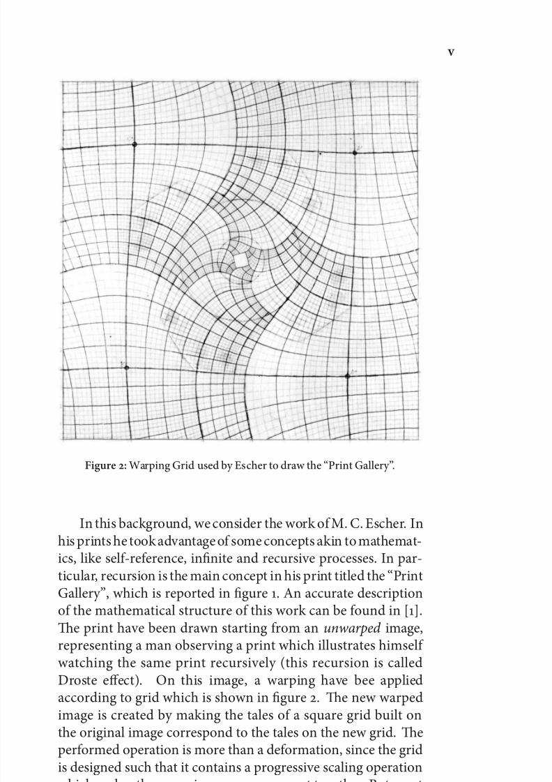
Figure : Warping Grid used by Escher to draw the “Print Gallery”.
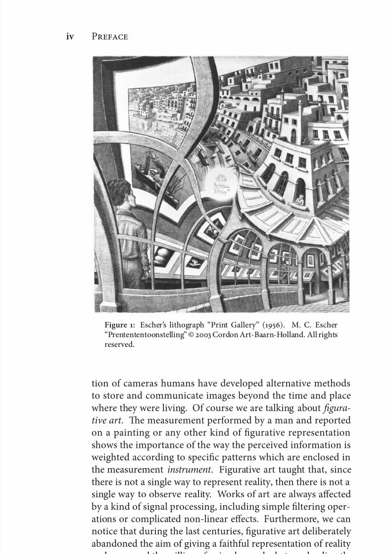
In this background, we consider the work of M. C. Escher. In
his prints he took advantage of some concepts akin to mathemat-ics, like self-reference, infinite and recursive processes. In par-ticular, recursion is the main concept in his print titled the “PrintGallery”, which is reported in figure . An accurate descriptionof the mathematical structure of this work can be found in [].
e print have been drawn starting from an unwarped image,representing a man observing a print which illustrates himself watching the same print recursively (this recursion is called
Droste effect). On this image, a warping have bee appliedaccording to grid which is shown in figure . e new warpedimage is created by making the tales of a square grid built onthe original image correspond to the tales on the new grid. eperformed operation is more than a deformation, since the gridis designed such that it contains a progressive scaling operationwhich makes the recursive spaces reconnect together. But apartfrom the scaling, we want to focus on the global effect that the

7/21/2019 Design and Computation of Warped Time-Frequency Transforms
http://slidepdf.com/reader/full/design-and-computation-of-warped-time-frequency-transforms 8/150
vi P
author’s point of view has given to the content. anks to thegrid, the tales of the image have been re-weighted accordingto a new sampling, so that some details which were not visible
and recognizable in the original version have been increased inimportance. A very interesting consideration to be done is thattrough the warping operation there is no increase in the globalinformation contained in the picture. Instead, the way the spaceof observation (the square frame) is split among the various partof the image has been modified.
It is quite intuitive that the problem of recovering the orig-inal image, which has been treated in [], is actually the sameproblem as drawing the warping image. In fact, one can assumethat the image in figure is the original one, and then draw anew image through a grid which nullify the effect of the grid infigure .
rough this example, we have already illustrated some of the basic properties and concepts behind the warping technique.Possible aims of such an operation can be easily imagine by comparison with the shown example. For instance, one couldneed to exalt some parts of a signal despite to others in orderto perform an accurate feature extraction. is approach canbe categorized as a direct application of a warping technique,since the starting point is the unmodified signal. Otherwise,it could be necessary to remove the effects of an acquisitionprocess which weights non-uniformly the different parts of theincoming signal. is approach would be labeled as an inverse
use of a warping technique, since the starting point is an already warped signal. As we suggested before, there is an intrinsicduality between the direct and the inverse approach.
e possibility of recovering the original signal by the war-ped one, that is the capability of define an inverse unwarpingwhich exactly inverts the direct one, is a very important issuewhen dealing with warping technique from a mathematicalpoint of view. Invertibility is the major problem which will be
considered in this work. Furthermore we will cope with the way the warping operation should to be designed, which means, by comparison with the Escher’s print example, what kind of curvesshould compose the grid in figure .
We finally report other hints suggested from Escher’s litho-graph. Although these consists in conceptual observations ra-ther than mathematical ones, they reveal to make sense inhindsight. We notice that the center of was le unpainted. We

7/21/2019 Design and Computation of Warped Time-Frequency Transforms
http://slidepdf.com/reader/full/design-and-computation-of-warped-time-frequency-transforms 9/150
vii
also learn from [] that the unwarped picture used by Escher wasnot complete, since the unpainted spot gives rise to an empty spiral. ese observations can be translated to our perspective
in the following metaphorical meaning. When warping a signalfrom a finite-dimensional domain to another finite-dimensionalone (i.e. a domain having an upper limited resolution), someinformation is necessarily discarded. Maybe a perfect recon-struction could be achieved anyway, but it involves somethingmore than merely inverting the steps employed for warping.

7/21/2019 Design and Computation of Warped Time-Frequency Transforms
http://slidepdf.com/reader/full/design-and-computation-of-warped-time-frequency-transforms 10/150

7/21/2019 Design and Computation of Warped Time-Frequency Transforms
http://slidepdf.com/reader/full/design-and-computation-of-warped-time-frequency-transforms 11/150
Contents
Preface iii
Introduction xiii
I eoretical Issues on Warped Transforms
Fourier and Warping Operators
. Fourier Operators . . . . . . . . . . . . . . . . . . . Frequency Warping Operators . . . . . . . . . . . . Conclusions . . . . . . . . . . . . . . . . . . . . .
e Frequency Warping Matrix . A Frequency Warping Map Example . . . . . . .
. Sparsity of a Warping Matrix . . . . . . . . . . . . . Time-Frequency Sampling . . . . . . . . . . . . .
. Smooth vs. non-Smooth Maps . . . . . . . . . . . . Conclusions . . . . . . . . . . . . . . . . . . . . .
II Algorithms for Frequency Warping
Nonuniform Fourier Transform . Introduction to NUFFT . . . . . . . . . . . . . . .
ix
7/21/2019 Design and Computation of Warped Time-Frequency Transforms
http://slidepdf.com/reader/full/design-and-computation-of-warped-time-frequency-transforms 12/150
x C
. Problem Statement . . . . . . . . . . . . . . . . . . Interpolation Approach . . . . . . . . . . . . . . . . SVD-based Proposed Algorithm . . . . . . . . . .
. Performances . . . . . . . . . . . . . . . . . . . . . . Conclusions . . . . . . . . . . . . . . . . . . . . .
Factorization of the Aliasing Matrix . Problem Statement and Methodology . . . . . . . . Heuristic Model of the Tails Matrix . . . . . . . . . Modeling of the Aliasing Matrix . . . . . . . . . . . Fast Warping Transforms . . . . . . . . . . . . . .
. Performances . . . . . . . . . . . . . . . . . . . . . . Conclusions . . . . . . . . . . . . . . . . . . . . . .A Mathematical Proofs . . . . . . . . . . . . . . . .
Frame Bounds Estimation . Discrete Frames . . . . . . . . . . . . . . . . . . . . Frame Bounds in Frequency Warping . . . . . . . . Error Estimation . . . . . . . . . . . . . . . . . . .
. Experimental Results . . . . . . . . . . . . . . . . . Conclusions . . . . . . . . . . . . . . . . . . . . .
III Applications on Ultrasound Signals
Ultrasonic Guided Waves . Introduction to Guided Waves . . . . . . . . . . .
. Dispersion-matched Warpograms . . . . . . . . . . Numerical and Experimental Results . . . . . . . . Conclusions . . . . . . . . . . . . . . . . . . . . .
Conclusions
Bibliography

7/21/2019 Design and Computation of Warped Time-Frequency Transforms
http://slidepdf.com/reader/full/design-and-computation-of-warped-time-frequency-transforms 13/150

7/21/2019 Design and Computation of Warped Time-Frequency Transforms
http://slidepdf.com/reader/full/design-and-computation-of-warped-time-frequency-transforms 14/150

7/21/2019 Design and Computation of Warped Time-Frequency Transforms
http://slidepdf.com/reader/full/design-and-computation-of-warped-time-frequency-transforms 15/150
Introduction
D the last years the relevance of time–frequency trans-
formations has widely grown in signal processing. esetechniques are commonly addressed to give a new representa-tion of a source signal. A time-frequency transformation couldbe adaptively defined in order to match the way the informationis recorded in the source signal. Alternatively, it could bedesigned to obtain a sparse representation for compression ordenoising applications. In some cases the two purposes couldmatch, i.e. the sparse representation also conveys some of thesource characteristics and implements a feature extraction. So,the ability of generating a flexible tiling of the time-frequency plane is a major issue. Many transformations have been intro-duced in order to accomplish this task, including the short timeFourier transform, the wavelet transform, filter banks and alltheir variations and mutual combination addressed to generalizetheir intrinsic characteristics [, ]. Nevertheless, such transfor-mations have some restrictive properties which make them notsuitable in some applications. In particular, some requirements,like fast computation and orthogonality, limit the degrees of freedom in choosing the proper time-frequency representation.
In order to approach the aim of an arbitrary time-frequency tiling, the application of a preliminary invertible transformationto reshape the frequency axis can be considered [, ]. istransformation is referred as frequency warping. e feature
xiii
7/21/2019 Design and Computation of Warped Time-Frequency Transforms
http://slidepdf.com/reader/full/design-and-computation-of-warped-time-frequency-transforms 16/150
xiv I
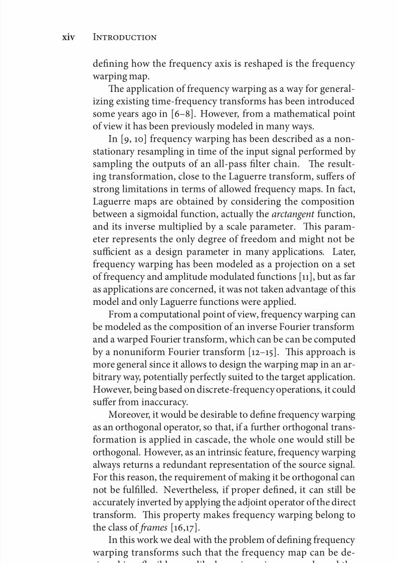
defining how the frequency axis is reshaped is the frequency warping map.
e application of frequency warping as a way for general-
izing existing time-frequency transforms has been introducedsome years ago in [–]. However, from a mathematical pointof view it has been previously modeled in many ways.
In [, ] frequency warping has been described as a non-stationary resampling in time of the input signal performed by sampling the outputs of an all-pass filter chain. e result-ing transformation, close to the Laguerre transform, suffers of strong limitations in terms of allowed frequency maps. In fact,Laguerre maps are obtained by considering the compositionbetween a sigmoidal function, actually the arctangent function,and its inverse multiplied by a scale parameter. is param-eter represents the only degree of freedom and might not besufficient as a design parameter in many applications. Later,frequency warping has been modeled as a projection on a setof frequency and amplitude modulated functions [], but as faras applications are concerned, it was not taken advantage of thismodel and only Laguerre functions were applied.
From a computational point of view, frequency warping canbe modeled as the composition of an inverse Fourier transformand a warped Fourier transform, which can be can be computedby a nonuniform Fourier transform [–]. is approach ismore general since it allows to design the warping map in an ar-bitrary way, potentially perfectly suited to the target application.
However, being based on discrete-frequency operations, it couldsuffer from inaccuracy.Moreover, it would be desirable to define frequency warping
as an orthogonal operator, so that, if a further orthogonal trans-formation is applied in cascade, the whole one would still beorthogonal. However, as an intrinsic feature, frequency warpingalways returns a redundant representation of the source signal.For this reason, the requirement of making it be orthogonal can
not be fulfilled. Nevertheless, if proper defined, it can still beaccurately inverted by applying the adjoint operator of the directtransform. is property makes frequency warping belong tothe class of frames [,].
In this work we deal with the problem of defining frequency warping transforms such that the frequency map can be de-signed in a flexible way, like by a piecewise approach, and theproperty of being inverted by the adjoint operator is satisfied up
7/21/2019 Design and Computation of Warped Time-Frequency Transforms
http://slidepdf.com/reader/full/design-and-computation-of-warped-time-frequency-transforms 17/150
xv
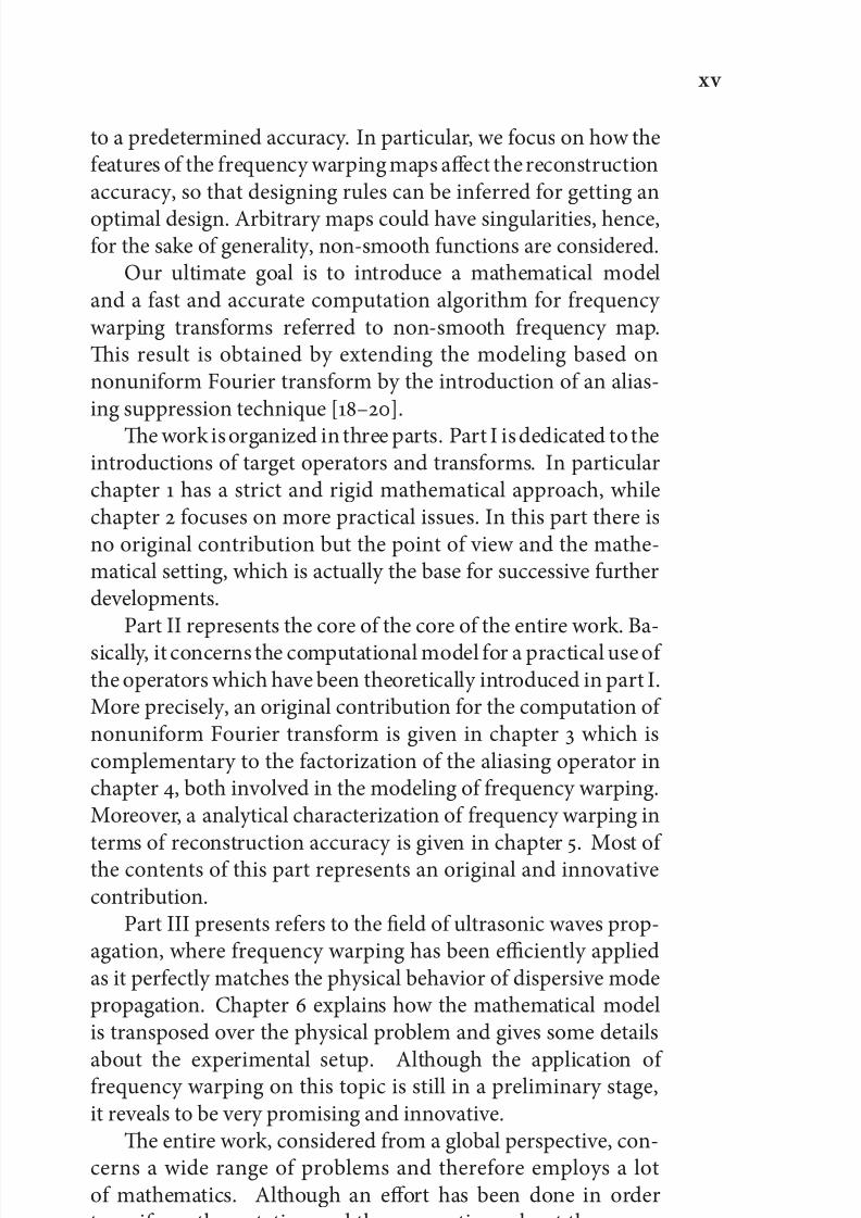
to a predetermined accuracy. In particular, we focus on how thefeatures of the frequency warping maps affect the reconstructionaccuracy, so that designing rules can be inferred for getting an
optimal design. Arbitrary maps could have singularities, hence,for the sake of generality, non-smooth functions are considered.
Our ultimate goal is to introduce a mathematical modeland a fast and accurate computation algorithm for frequency warping transforms referred to non-smooth frequency map.is result is obtained by extending the modeling based onnonuniform Fourier transform by the introduction of an alias-ing suppression technique [–].
e work is organized in three parts. Part I is dedicated to theintroductions of target operators and transforms. In particularchapter has a strict and rigid mathematical approach, whilechapter focuses on more practical issues. In this part there isno original contribution but the point of view and the mathe-matical setting, which is actually the base for successive furtherdevelopments.
Part II represents the core of the core of the entire work. Ba-sically, it concerns the computational model for a practical use of the operators which have been theoretically introduced in part I.More precisely, an original contribution for the computation of nonuniform Fourier transform is given in chapter which iscomplementary to the factorization of the aliasing operator inchapter , both involved in the modeling of frequency warping.Moreover, a analytical characterization of frequency warping in
terms of reconstruction accuracy is given in chapter . Most of the contents of this part represents an original and innovativecontribution.
Part III presents refers to the field of ultrasonic waves prop-agation, where frequency warping has been efficiently appliedas it perfectly matches the physical behavior of dispersive modepropagation. Chapter explains how the mathematical modelis transposed over the physical problem and gives some details
about the experimental setup. Although the application of frequency warping on this topic is still in a preliminary stage,it reveals to be very promising and innovative.
e entire work, considered from a global perspective, con-cerns a wide range of problems and therefore employs a lotof mathematics. Although an effort has been done in orderto uniform the notation and the conventions about the repre-sentation of signals and operators, the work is not completely
7/21/2019 Design and Computation of Warped Time-Frequency Transforms
http://slidepdf.com/reader/full/design-and-computation-of-warped-time-frequency-transforms 18/150

7/21/2019 Design and Computation of Warped Time-Frequency Transforms
http://slidepdf.com/reader/full/design-and-computation-of-warped-time-frequency-transforms 19/150

7/21/2019 Design and Computation of Warped Time-Frequency Transforms
http://slidepdf.com/reader/full/design-and-computation-of-warped-time-frequency-transforms 20/150
7/21/2019 Design and Computation of Warped Time-Frequency Transforms
http://slidepdf.com/reader/full/design-and-computation-of-warped-time-frequency-transforms 21/150
P
Ieoretical Issues on
Warped Transforms

7/21/2019 Design and Computation of Warped Time-Frequency Transforms
http://slidepdf.com/reader/full/design-and-computation-of-warped-time-frequency-transforms 22/150
7/21/2019 Design and Computation of Warped Time-Frequency Transforms
http://slidepdf.com/reader/full/design-and-computation-of-warped-time-frequency-transforms 23/150
C
Fourier and Warping
Operators
T chapter will present the notation which will be used in
the rest of the work. More in details, we will refer to eithertime-continuous and time-discrete signals and we will providedefinitions for mathematical operators applied to both of them.In particular, we will mainly deal with time-frequency operators,so a major space will be dedicated to fixing the notation andthe conventions about the Fourier transform. Finally we willintroduce the frequency warping operator, which will be thestarting point for the further developments of the rest of thework.
Both Fourier and warping operator will be presented inthe continuous-time, discrete-time continuous-frequency anddiscrete-time discrete-frequency cases. A particular attentionwill be dedicated to invertibility and reconstruction accuracy.In this framework we will recall the sampling theorem and theduality between time and frequency domains. As a conclusion,we will introduce a additive decomposition of the time-discretefrequency warping operator in its frequency sampled approxi-mation and an aliasing term. Both these operators will be deeply discussed in next chapters.
As a convention, signals will be represented in lowercaseitalic letters, while operators will be represented by boldface up-percase letters. We deliberately introduce an ambiguity betweenthe representation of the operators and their kernels.

7/21/2019 Design and Computation of Warped Time-Frequency Transforms
http://slidepdf.com/reader/full/design-and-computation-of-warped-time-frequency-transforms 24/150
C . F W O
. Fourier Operators
We start by reviewing the Fourier transform and its main prop-
erties, which are supposed to be well-known to the reader. So,the purpose of this section is to present an approach based onoperators for the derivation and description of Fourier trans-forms. is may be useful to suggest a comparison to linearalgebra, which will be deeply exploited in this work. Moreover,this short summary on Fourier transforms may serve as anexercise to get acquire familiarity with the operators approach.
From a practical point of view, we first introduce the contin-
uous Fourier transform, then we derive the Fourier transformfor discrete-time signals and finally the discrete transform inboth time and frequency. e aim is to maintain a referenceto the continuous operator in the definition of the discretetransforms, so that, when warping will be applied, the derivationto discrete case will be straightforward.
.. Continuous-Time OperatorsIn order to illustrate this representation, we start by consideringthe Fourier F transform applied on a continuous signal s:
F ∶ L(R) → L(R), s(t ) ↦ s( f ) = R
s(t )e− jπt f dt
so, the operator kernel is simply given by:
F( f , t ) = e
− jπt f
.In compact operator notation the Fourier transform is repre-sented by:
s = Fs
e adjoint operator will be represented by the † subscript:
F† ∶ L(R) → L(R), s( f ) ↦
[F†s
](t
) =
R
s
( f
)e− jπt f d f
and the operator kernel is obtained by complex conjugating F .e Fourier operator is unitary, i.e. its inverse operator is givenby the adjoint one:
F− = F†
which is easily verified by considering:
[F†F
](t , τ
) =
R
e− jπ t f e jπτ f = R
e− jπ (t −τ ) f = δ
(t − τ
)
7/21/2019 Design and Computation of Warped Time-Frequency Transforms
http://slidepdf.com/reader/full/design-and-computation-of-warped-time-frequency-transforms 25/150
.. F O
that, in compact notation, is:
F†F = I
where I is the identity operator.
.. Nyquist eorem Revisited
Now we want to consider discrete-time signals. In order to dothis, we first introduce the sampling operator D (where D staysfor Delta):
D ∶ L(R) → ℓ (Z), s(t ) ↦ [Ds](n) = R
s(t )δ (t − n)dt
whose kernel is simply given by:
D(n, t ) = δ (t − n).
In order to transform a discrete-time signal, the Fourier operatorhas to be sampled as well, so that we should consider:
[FD†](t , f ) = R
e− jπt f δ (t − n)dt = e− jπn f .
Now we suppose that the considered signal is band-limited, withbandwidth equal to , then the sampling operation does notcause a loss in information. Sampling just cause a periodic
repetition in the frequency domain. Let us show this well-known property by the operator notation. e sampling can berepresented in the frequency domain as:
FD†Ds
where the operator D†D can be explicitly computed:
[D†
D](t , τ ) = n∈Z δ (t − n)δ (τ − n) = δ (t − τ ) n∈Z δ (t − n)which is actually a diagonal operator whose diagonal is givenby a Dirac comb. We remind that the Dirac comb can beequivalently represented by its Fourier series:
n∈Z
δ (t − n) = n∈Z
e jπnt
7/21/2019 Design and Computation of Warped Time-Frequency Transforms
http://slidepdf.com/reader/full/design-and-computation-of-warped-time-frequency-transforms 26/150
C . F W O
so we get:
[FD†Ds
]( f
) = R
e− jπt f
n∈Ze jπnt s
(t
)dt
= n∈Z
R
e− jπt ( f −n)s(t )dt = n∈Z
s( f − n).
We can introduce the periodic repetition operator R such that:
R ∶ L(R) → L∞(R), s(ξ ) ↦ [Rs]( f ) = R
s(ξ )Z
δ (ξ − f +n)whose kernel is represented by:
R( f , ξ ) = n∈Z
δ (ξ − f + n).
is equivalence can be finally set:
FD†D = RF
which means that in order to invert the sampling operationwe must be able to invert the periodic repetition. Normally periodic repetition is not an invertible operation, unless theconsidered signal is band-limited. In particular we are interestedin baseband signals, so we just suppose that the input signalhas non-zero amplitude only in the interval [− ⁄ , ⁄ ]. By thishypothesis, we can invert the periodic repetition by windowingthe spectrum with a rectangular filter H:
H( f , ξ ) = δ ( f − ξ )[H (ξ + ) − H (ξ − )]where H is the Heaviside function. So, in case of baseband band-limited signals, the operator:
F†HFD†D
behaves like an identity operator. In order to specify this result,we first consider:
[F†HF](t , τ ) = R
e jπ f t [H ( f + ) − H ( f − )]e− jπ f τ d f
= ⁄
−⁄e jπ f (t −τ )d f
= sinc
(t − τ
)

7/21/2019 Design and Computation of Warped Time-Frequency Transforms
http://slidepdf.com/reader/full/design-and-computation-of-warped-time-frequency-transforms 27/150
.. F O
and then define the resulting operator as:
S
(t , τ
) = sinc
(t − τ
)so that, the global operation performed on the input signal s canbe represented as:
SD†D.
Now we notice that SD† can be written as an interpolator:
SD†(t , n) = R
sinc(t − τ )δ (τ − n)dτ = sinc(t − n).
It results that this inversion procedure gives as output the input
signal samples interpolated by a sinc function, so it recovers theoriginal signal if the signal could actually be expressed as a linearcombination of shied sinc functions. Finally we consider thisequality:
SD†DS = F†HRHF.
Since HRH is equal to H, we conclude that:
SD†DS = S. (.)
which means that, given a generic signal, the subspace identifiedby S can be recovered aer sampling by applying SD†.
.. Discrete-Time Fourier Operators
Aer having explained how to pass from continuous to discretedomain, we can deal with discrete-time signals. So, from thispoint forward, s will represent a sequence in ℓ
(Z
). e Fourier
transform has to be redefined for the new input domain. Inparticular, it could be desirable to define such that the inverseoperator is equal to the transpose one.
Let us apply a sampling on both sides of equation (.):
DSD†DS = DS
which tells us that the subspace identified by DS is invariantrespect to the application of DSD†. Since we consider as input
ℓ (Z), which is generated by DS, the operator to evaluate isDSD†:
[DSD†](m, n) = R
δ (t − n) R
sinc(t − τ )δ (τ − m)dτdt
= R
δ (t − n)sinc(t − m)dt
= sinc
(n − m
)
7/21/2019 Design and Computation of Warped Time-Frequency Transforms
http://slidepdf.com/reader/full/design-and-computation-of-warped-time-frequency-transforms 28/150
C . F W O
which means that DSD† is equal to the identity operator respectto ℓ (Z):
DSD† = I
therefore the Fourier operator and its adjoint can be put aer D:
DSF†FD† = I.
e direct Fourier transform for discrete-time signals can bedefined as follows:
FD† ∶ ℓ
(Z
) → L∞
(R
), s
(n
)↦ s
( f
) =
n∈Z
s
(n
)e− jπn f (.)
whose kernel is merely given by:
[FD†]( f , n) = e− jπn f
e inverse operator can be defined by:
[FD†
]− = DSF† = DF†H
such that:
[FD†]− ∶ L(R) → ℓ (Z), s( f ) ↦ s(n) =
s( f )e jπn f dt
where the interval [, ] has been equivalently considered ratherthan [− ⁄ , ⁄ ].
We point out that, in the inverse operator, the purpose of
operator DS aer operator F†
is to reduce a Dirac comb of thiskind:
n∈Z
s(n)δ (t − n)whose energy is infinite, to a finite energy sequence troughsubstituting the Dirac impulses by Kronecker symbols. So theFourier transform of a sequence is intrinsically periodic, thewindowing operation performed by operator H accomplishes
only computational needs. For this reason, we prefer to rep-resent the Fourier transform of a discrete-time signal and itsinverse by the operator described above.
Nevertheless, it could be convenient as well to define theFourier transform so that the inverse operator is given by itsadjoint. In order to do this, we consider:
DF†HFD† = DF†HHFD† =
[DF†H
][HFD†
]

7/21/2019 Design and Computation of Warped Time-Frequency Transforms
http://slidepdf.com/reader/full/design-and-computation-of-warped-time-frequency-transforms 29/150
.. F O
and since H† = H, we could set:
HFD† ∶ ℓ
(Z
)→ L
([,
)), s
(n
)↦ s
( f
) =
n∈Z
s
(n
)e− jπn f dt
(.)as an alternative definition of Fourier transform. e kernel isobviously the same as in the previous definition, since operatorH only affects the codomain. Independently on the adopteddefinition, the discrete-time operator will be referred as FD.
From a practical point of view, considering the entire fre-quency axis as output domain rather than a single period, does
not imply substantial differences. Instead, from a theoreticalpoint of view, it will have important implications when fre-quency warping will be applied. In fact, when an operator isapplied on the frequency domain, even if the axis is restrictedto a single period, the periodicity has to be taken into accountfor rightly modeling the effects of the considered operator andpotentially for designing it according to some optimality criteria.
.. Discrete Fourier Operator
Now we want to introduce discrete operators in both timeand frequency domains. e approach which will be followedis quite the same as the one used to introduce discrete-timeoperators.
In time domain we considered a sampling step equal to .Because of it, the frequency domain period is equal to as well.
So, it is quite evident that in the frequency domain we mustconsider a sampling step smaller than . Moreover, in order tomaintain periodicity, the sampling step must be contained in theperiod an integer number of times. erefore we will assumethat the sampling step is equal to N , or rather the period issampled in N different points. e sampling operator has tomodified so that it performs this task and will be representedas DN :
DN ∶ L∞(R) → ℓ ∞(R),
s( f ) ↦ [DN s](k) = R
s( f )δ ( f − kN )d f
whose kernel is given by:
DN
(k , f
) = δ
( f − k
N
).
7/21/2019 Design and Computation of Warped Time-Frequency Transforms
http://slidepdf.com/reader/full/design-and-computation-of-warped-time-frequency-transforms 30/150
C . F W O
Now, we apply this sampling operator on the le of the Fourieroperator and on the right of the adjoint one:
DSF†
D†N DN FD
†
. (.)
e operator D†N DN roughly behaves like the operator D† D, that
is:
[D†N DN ]( f , ξ ) =
k∈Z
δ ( f − kN )δ (ξ − kN )= δ ( f − ξ )
k∈Z
δ ( f − kN )again, the Dirac comb can be represented by:
k∈Z
δ ( f − kN ) = N k∈Z
e jπ f kN
so that, from F†D†N DN F we get:
[F†D†
N DN F
](t , τ
) =
R
e jπ f t N k∈Z
e jπ f kN e− jπ f τ
= N k∈Z
R
e jπ f (t −τ +kN ) = N k∈Z
δ (t − τ + kN ).
e resulting operator performs a repetition with step equalto N , In order to complete the chain (.), we still miss theD† operator on the right and the DS operator on the le. By applying D† we get:
[F†D†N DN FD†](t , n) =
R
N k∈Z
δ (t − τ + kN )δ (τ − n)dτ
= N k∈Z
δ (t − n + kN )while by applying [DS](m, t ) = sinc(t − m) on the right we get:
[DSF†D†
N DN FD†
](m, n
) =
R
sinc(t −m)N k∈Z
δ (t −n+kN )dt = N k∈Z
sinc(n−m−kN )where the sinc functions, being sampled on integer values, be-haves like Kronecker symbols. e obtained operator representsa discrete periodic repetition which will be referred as RN :
RN = N −DSF†D†N DN FD† .
7/21/2019 Design and Computation of Warped Time-Frequency Transforms
http://slidepdf.com/reader/full/design-and-computation-of-warped-time-frequency-transforms 31/150
.. F O
As expected, the sampling in the frequency domain causesa periodic repetition in discrete time domain. In order to avoidloss in information, the following operator should maintain the
input signal unchanged:
HN RN
where HN is suitable rectangular discrete-time window of lengthequal to N . So, the following statement is surely satisfied:
HN RN HN s = HN s
and we infer that the signal must be time-limited to an intervalequal or smaller than N samples.
By considering as input domain the space generated by HN ,we can now define the discrete Fourier transform as:
DN FD† ∶ RN → ℓ ∞(Z), s(n) ↦ s(k) = n∈Z N
s(n)e− jπnkN
where ZN is a set of N consecutive integers. e inverse trans-
form is expressed by:[DN FD†]− = N −DSF†D†N = N −DF†HD†
N
and it acts on the discrete Fourier transformed signal s as fol-lows:
[DN FD†]− ∶ ℓ ∞(Z) → RN ,
s
(k
)↦ s
(n
) = N −
k∈Z N s
(k
)e jπnkN .
Here, the set ZN is not necessarily the same set used in the directtransform. A standard choice is to consider for both the sets:
ZN = , , . . . , N − but, as said before, other choices are allowed.
Again, we could redefine the direct Fourier operator such
that the output domain is limited in frequency, i.e. RN :
DN HFD† ∶ RN → RN , s(n) ↦ s(k) =
n∈Z N
s(n)e− jπnkN
whose inverse is represented by its adjoint multiplied by theconstant being the input dimension:
[DN HFD†
]†
[DN HFD†
] = N IN
7/21/2019 Design and Computation of Warped Time-Frequency Transforms
http://slidepdf.com/reader/full/design-and-computation-of-warped-time-frequency-transforms 32/150
C . F W O
where IN is the identity operator for a RN .e discrete Fourier transform operator will be represented
as FD N D , either if the codomain is the entire frequency axis or a
single period.
. Frequency Warping Operators
In this section we introduce the warping operators. e pre-sentation follows the flow which has been used for the Fourieroperators. So, we start from the continuous case, then introduce
the sampling of the time axis and finally derive the the samplingof both time and frequency axis. Preliminarily, the warping of ageneric axis as an intrinsic transformation will be considered,then it will be transposed to the frequency axis. Even if thewarping is performed in the frequency domain, the frequency warping operator is defined so that it acts in the time-domain.So, the introduced deformation is not directly observable andrecognizable in the time-domain.
.. Unitary Operators
Roughly speaking, a unitary operator is an operator such thatits inverse is given by the adjoint one. Unitariness is alwaysa desirable property for an operator, since it carries out someadvantages which can be very important in signal processing.More in details, an operator U is said to be unitary the following
three condition are satisfied:
• Linearity.Given two constants a , b ∈ R and two functions or vectorss and s, linearity is satisfied if:
U[as + bs] = aUs + bUs
• Suriectivity.
is property, also said non-singularity, ensures that noinput function is transformed in the function:
Us = ⇔ s =
• Isometry.is property consists in preserving distances:
Us
=
s

7/21/2019 Design and Computation of Warped Time-Frequency Transforms
http://slidepdf.com/reader/full/design-and-computation-of-warped-time-frequency-transforms 33/150
.. F W O
Linearity is normally satisfied for most of the operators whichare used in time-frequency analysis. An example of operatorwhich does not verify the surjectivity property is a filter, which
by definition nullify all the information carried by specifiedfunctions or vectors. Examples of transformations which fulfillthe isometry property are the time-shi, the frequency-shi ormodulation and the scaling.
By considering the isometry property, for Us we get:
Us = [Us]†[Us] = s†U†Us
so that, the isometry is satisfied if and only if:
U− = U† . (.)
which is the property announced at the beginning. We remindthat in the previous section, when we defined the Fourier op-erators, we always provided a definition satisfying the unitary property. As far as warping is concerned, we will attempt to thesame as for Fourier operators.
Since the norm of s is given by the square root of the scalar
product between s and itself, it follows that the scalar productbetween two functions or vectors s and s is invariant respectto the application of a unitary operator:
[Us]†[Us] = s† U†Us = s†
s .
is formulation suggests the way a unitary operator can beused. Let us suppose to have another unitary operator, forexample the Fourier operator F. e composed operator FU is
still unitary, since:[FU]†[FU] = U†F†FU = U†U = I.
So, the analysis performed by F can be modified through theapplication of U, which could be applied either to the right
F or to le of the input function or vector. e first optionwould involve a modification on the operator F, so it may benot completely painless. erefore, it should be much more
convenient to apply it preliminarily on the input signal. We pointout that, if the considered operator performs for example a shitowards le and we want to obtain such a modification on thebases vectors, the transformation to be applied on the signal isthe inverse one, or rather the adjoint one, In fact, if we force U
to act on F rows from the right, we get:
FUs =
[[FU
]†
]†s =
[U†F†
]†s. (.)
7/21/2019 Design and Computation of Warped Time-Frequency Transforms
http://slidepdf.com/reader/full/design-and-computation-of-warped-time-frequency-transforms 34/150
C . F W O
.. Continuous Warping Operator
Here we want to introduce the concept of deformation of a
continuous function. Intuitively, to get a deformation of afunction one has to introduce a deformation on its axis. ismeans that we must set a function w, such that it maps the oldaxis x to the new axis w(x ):
w ∶ R → R, x ↦ w(x ).
In previous sections we oen focused on invertibility. To get aninvertible warping operator, the function w must be an invertible
function, that is:
w > a.e. ⇒ ∃w− , w−(w(x )) = x (.)
where w represents the first derivative of w while w− representsthe functional inverse. Starting from w, we introduce the trans-formation which substitutes the axis x of an input function s(w)by w
(x
). is is actually the composition of s and w:
Ws = [s w](x ) = s(w(x )).
e kernel of this operator can be described as follows:
W(x , y ) = δ (w(x ) − y )in fact:
[Ws
](x
) =
R
δ
(w
(x
)− y
)s
( y
)d y = w
(s
(x
)).
is operator is candidate to become the warping operator. Tobe elected, it must be linear, surjective and isometric. e firstproperty is straightforward:
W[as + bs] = aWs + bWs a, b ∈ R.
Surjectivity is guaranteed by (.). In fact, being s equal to
only on certain intervals or points, it is transformed in the zerofunction only if the composition with w makes s(w(x )) returnthe only the zero values of s(x ). is is impossible, since w(x ),having positive derivative, maps x onto itself.
To verify the isometry property, we apply the adjoint opera-tor in order to recover the identity:
[W†W
](z , y
)=
R
δ
(z − w
(x
))δ
(w
(x
)− y
)dx
7/21/2019 Design and Computation of Warped Time-Frequency Transforms
http://slidepdf.com/reader/full/design-and-computation-of-warped-time-frequency-transforms 35/150
.. F W O
then we should set the following integration variable change:
w
(x
) = ξ ⇒ w
(x
)dx = d ξ ⇒ dx =
w(w−
(ξ ))d ξ (.)
which gives:
[W†W](z , y ) = R
δ (z − ξ )δ (ξ − y )
w(w−(ξ ))d ξ
=
w(w−(z ))δ (z − y ).
So, the isometry property is not verified, but this negative resultsuggest us how to modify the expression of W. e integralshould contain a factor equal to w(x ), so that, by posing w(x ) =ξ , w(x )dx would be simply substituted by d ξ . erefore we set:
W ∶ L(R) → L(R), s( y ) ↦ [Ws](x ) = w(x )s(w(x ))whose kernel is:
W(x , y ) = w(x )δ (w(x ) − y ).Now the isometry property is easily verified:
Ws = R
w(x )s(w(x ))dx = R
s(ξ )d ξ = s
where the above substitution (.) has been used.Now we want to focus on the inverse operator W− . As we
verified, it can be expressed by the adjoint operator. Anyway,
we did not take advantage of the functional inverse w− , whichcould serve as a mapping function as well. So we consider:
W(z , x ) = w−(z )δ (w−(z ) − y )
which, combined with W, gives:
[ WW
](z , y
) =
R
w−
(z
)w
(x
)δ
(w−
(z
)− x
)δ
(w
(x
)− y
)dx
= w−(z )w(w−(z ))δ (w(w−(z )) − y )= δ (z − y )
where we exploited (.) for the expression of w− . Finally weobtained the identity operator, which means that:
W = W† = W− .

7/21/2019 Design and Computation of Warped Time-Frequency Transforms
http://slidepdf.com/reader/full/design-and-computation-of-warped-time-frequency-transforms 36/150
C . F W O
.. Continuous Frequency Warping Operator
Now we want to apply the continuous warping operator W
in order to get a deformation of the frequency axis throughan operator to be used in the time-domain. So, basically, theoperator has to be applied between a Fourier transform and aninverse Fourier transform. is operator will be referred as WF ,where the subscript points that the warping is executed in thetransformed domain. We get:
WF = F†WF.
Before going on computing its kernel, we introduce the interme-diate operator FW :
FW = WF
whose kernel is given by:
FW
( f , t
) =
R
w
( f
)δ
(w
( f
)− ξ
)e− jπ ξt d ξ
= w( f )e− jπw ( f )t .
FW is still a unitary operator, being the composition of unitary operators. So, WF is represented as:
WF = F†FW .
having the following kernel:
WF(t , τ ) = R
w( f )e− jπw ( f )τ e jπ f t d f
= R
w( f )e jπ ( f t −w ( f )τ )d f
and the operator can be formally defined as:
WF ∶ L
(R) → L
(R), s(τ ) ↦ [WFs](t ) == R
s(τ ) R
w( f )e jπ ( f t −w ( f )τ )d f d τ .
We point out that this operator, involving continuous operation,can not be analytically computed for a generic signal s, since, onthe other hand, not even the continuous Fourier transform of ageneric signal can be analytically performed.
7/21/2019 Design and Computation of Warped Time-Frequency Transforms
http://slidepdf.com/reader/full/design-and-computation-of-warped-time-frequency-transforms 37/150
.. F W O
We underline that WF is still a unitary operator. Anotherthing to be taken into account is the shape to be given to thewarping function w. Since we normally deal with real input
signals, it may be required that the output is real as well. So, thisrequirement must be imposed on the shape of w. Intuitively, be-ing the Fourier transformed of a real signal symmetric respect tothe origin, we should impose that this symmetry is maintainedaer the application of frequency warping. In a simpler fashion,we can impose that the real part and the imaginary part of theoperator FW kernel are even and odd respectively:
FW( f , t ) = FW∗(− f , t ) w( f )e− jπw ( f )t = w(− f )e jπw (− f )t
which is verified if:
w( f ) = −w(− f ). (.)
that is, w must be an odd function in order to make WF trans-
form a real signal in a real signal. Since w is also an increasingfunction, it follows that the origin of the frequency axis is a fixedpoint of the w map, that is w() = .
.. Discrete-Time Frequency Warping
For discrete-time signals, the procedure to be used to obtain thecorresponding frequency warping operator is the same as for
the continuous time case. e warping operator has to be putbetween a Fourier transform and an inverse Fourier transform.
As far as the Fourier transform of a discrete-time signal isconcerned, we can choose between definition (.) and (.). Inorder to maintain the entire frequency axis as codomain, wechoose the first definition, so that:
WFD = DSF†WFD† = DSWFD†
is the target operator. e subscript FD stays to represent thatW is enclosed between a Fourier transform and a passage to asampled domain.
Obviously, the warping map w has to be properly redefinedin order to adapt to the periodicity of the Fourier transform of discrete-time signal. More precisely, we require the operatorDS on the right not to cause loss of information, or rather, we
7/21/2019 Design and Computation of Warped Time-Frequency Transforms
http://slidepdf.com/reader/full/design-and-computation-of-warped-time-frequency-transforms 38/150
C . F W O
want W F D to give as output a sequence of Dirac impulses. Toget this result, the warping map has to be defined as a functionrespecting conditions (.) and (.) and in addition, it must
preserve periodicity. So, the effect of WFD† is:
[WFD†s]( f ) = w( f ) n∈Z N
s(n)e− jπnw ( f )
and we must impose:
[WFD†s
]( f
) =
[WFD†s
]( f + k
) k ∈ Z
which can be rewritten as: w( f )e− jπnw ( f ) = w( f + k)e− jπnw ( f +k) .
We remind that a complex exponential is a periodic functionwhose period is equal to jπ , so we set:
w
( f
) = w
( f + k
)+ nk k , nk ∈ Z
which also satisfies the equivalence of the square root factors.From the above equation, we derive:
w(k + ) − w(k) = n k+ − nk
with n = since w() = . Moreover, limited to the interval
[,
], w has to be an invertible map, so for sure we have w
(
) = .
en it follows:
w( f + k) = k + w( f ) k ∈ Z.
We also remind the property (.), which causes:
w( f ) = −w(− f ) = −w(− f + ) +
where, by posing f =
, we get:
w() = −w(− + ) + ⇒ w() = .
Finally, we conclude that in the discrete-time case, the warpingmap is designed such that it has an infinite number of fixedpoints in (k , k)with k ∈ Z. In addition, if the resulting operatortransforms real signals into real signals, than the map also hasfixed points in
(k +
, k +
) with k ∈ Z and, if considered in
7/21/2019 Design and Computation of Warped Time-Frequency Transforms
http://slidepdf.com/reader/full/design-and-computation-of-warped-time-frequency-transforms 39/150
.. F W O
the interval [k , k + ], it is antisymmetrical respect to the pointk + .
Now we can give the formal definition of WF D :
WFD ∶ ℓ (Z) → ℓ (Z), s(n) ↦ [WFD s](m) ==
n∈Z
s(n)
w( f )e jπ (m f −nw ( f ))d f
where the kernel of WFD can be actually considered as a matrixof infinite dimension:
WFD(m, n) =
w( f )e jπ (m f −nw ( f ))d f . (.)
Again, we point out that the obtained operator is unitary,since it can be inverted by the adjoint operator. Althoughhaving discrete input and output, the operator WFD can not bepractically used. is is due to two facts:
• the computation of WFD entries requires the calculationof an integral;
• input and output can not be infinite-dimensional.
e second issue can be solved by limiting the input and theoutput domain in a proper way, trying to preserve the unitary
property. Instead, the first issue has to be solved by finding an al-gorithm to compute the matrix entries with discrete operations.
As a concluding remark, we show that the operator WF D canbe synthetically represented as a discrete-time warped Fouriertransform FWD = WFD and an adjoint discrete-time Fouriertransform (the inverse operator should be preferred to the ad- joint one, since it is independent on the bivalence introducedfor the definition of FD). So, it results:
WFD = FD†FWD .
e operator FWD , being the composition of the unitary opera-tors W and FD , is still unitary:
FWD†FWD = I.
7/21/2019 Design and Computation of Warped Time-Frequency Transforms
http://slidepdf.com/reader/full/design-and-computation-of-warped-time-frequency-transforms 40/150
C . F W O
.. Frequency Warping Transform
As a first step, the domain of the operator WFD has to be
limited. To do this, we exploit the operator HN , which hasbeen previously introduced. e usage of this operator will bedeliberately done with a subtle ambiguity. In some cases, HN
just turns to the input samples which are indexed outside of a specified interval of consecutive integers, so it behaves like asingular transformation from ℓ (Z) to itself. In other cases, HN
has the role of limiting the domain to the interval of consecutiveintegers specified before, so it behaves like a transformation
from ℓ
(Z) to R
N
. So, the adopted behavior will be clear timeto time by the context.
Now we introduce the following operator:
WFD HN ∶ RN → ℓ (Z), s(n) ↦ [WFD HN s](m) =
= n∈Z N
s(n)
w( f )e jπ (m f −nw ( f ))d f
where ZN is a suitable set of N consecutive integers. isoperator presents a significant difference in comparison to theoperators introduced so far. In fact, previously, we alwaysprovided a definition for the operators such that the inversetransform is equal to the adjoint one. In this case, dealing with arectangular matrix of dimension ∞ × N , the inverse matrix doesnot exist. Nevertheless, thanks to the unitary property of WFD ,we have:
[WFD HN ]†[WFD HN ] = HN W†FD WFD HN = IHN = IN .
e above modification is painless, since it does not alter theproperty of perfectly recovering the input signal starting fromthe transformed one by the application of the adjoint operator.We point out that this relationship is not commutative, that is:
[WFD HN
][WFD HN
]† = WFD HN W
†FD ≠ I
since, because of HN , the degrees of freedom are decreased from
∞ to N , that is [WFD HN ]† is a singular not invertible operator.So, for a finite computation, the input length must be limited.
is is quite intuitive, since frequency warping is a time-varianttransformation (time-variance is easily deduced by noting thatin the frequency domain WF D is equal to W and not to adiagonal operator).
7/21/2019 Design and Computation of Warped Time-Frequency Transforms
http://slidepdf.com/reader/full/design-and-computation-of-warped-time-frequency-transforms 41/150
.. F W O
We must introduce a further modification in order to copewith the infinite output length. As it has been done on thedomain, we limit the codomain by applying an operator HM
on the le. e windowing matrix H M is built like HN , but itmay refer to a suitable set of consecutive integers whose lengthis equal to M . For the moment, there is no need to put any constraint on M . So, we set:
W MN = H M WFD HN = H M DSF†WFD†HN
where the subscript MN means that W has been enclosed be-
tween a Fourier transform, a sampling and finally a truncationto a M × N matrix. Formally, the operator is represented by:
W M N ∶ RN → R
M , s(n) ↦ [W M N s](m) ==
n∈Z N
s(n)
w( f )e jπ (m f −nw ( f ))d f m ∈ Z M .
Unfortunately, independently on the chosen value of M , theoperator W M N loses the property of being inverted by its adjointoperator. In order to represent this loss, we define:
E M N = WFD HN − W M N
which represents the complement matrix to W MN respect tomatrix WFD HN . It has the meaning of error operator whichoccurs when matrix WFD HN is substituted by W M N . So, the
composition of W M N and its adjoint gives:
W† M N W M N = IN − E†
MN E M N .
which, as said before, differs from the identity. Nevertheless,in the next chapters it will be shown how this operator can beused with a sufficient degree of precision. For the moment wedo not deal with this problem and assume W M N to be the target
operator to be modeled.
.. Sampled Frequency Warping Transform
e entries of matrix W M N are equal to the entries of matrix
WFD limited to the rectangle given by the cartesian productZ M ×ZN . So, from a practical point of view, the new operator does notdiffer from the previous one in a significant manner. Instead,
7/21/2019 Design and Computation of Warped Time-Frequency Transforms
http://slidepdf.com/reader/full/design-and-computation-of-warped-time-frequency-transforms 42/150
C . F W O
from a conceptual point of view, the new operator allows someadvantages. Being finite-dimensional, it may be possible tomodel the continuous integral by a discrete procedure.
Retracing the way Fourier operators were introduced, wefirst considered continuous operators, the we sampled the timeaxis and finally we sampled the frequency axis. So, now we in-troduce a sampling on the frequency axis of frequency warpingoperator as well. It is pretty obvious that this operation can notbe painless. Since warping was originally defined on a contin-uous axis, sampling will probably alter the unitary property of warping. Nevertheless, as we said before about with regard to theapplication of operators H M , we will cope with reconstructionproblem in the next chapters.
Let us consider the following:
DSF†D† M D M WFD†
which is operator WFD on which a sampling in frequency hasbeen applied. Intuitively, the sampling should produce a peri-odic repetition in time. To demonstrate this, we try to force thepresence of operator R M . So, we evaluate the dual relationshipof (.):
RHR = R
which means that a periodic space is invariant respect to therestriction to subspace H followed by periodic repetition. So RH
behaves like an identity operator respect to a periodic input. Itsame can be rewritten in the following way:
RH = FD†DSF† .
Since the operator WFD produces a periodic output, RH can beapplied to it without any effects:
DSF†
D† M D M WFD
†
= DSF†
D† M D M [RH]WFD
†
= DSF†D† M D M [FD†DSF†]WFD†
= [DSF†D† M D M FD†][DSF†WFD†]
= M R M WFD .
By applying of a limiter H M and HN on the le and on theright respectively, we can formally define the sampled frequency
7/21/2019 Design and Computation of Warped Time-Frequency Transforms
http://slidepdf.com/reader/full/design-and-computation-of-warped-time-frequency-transforms 43/150
.. C
warping transform:
W M N ∶ R
N → R M , s
(n
)↦
[W M N s
](m
) =
n∈Z N
s(n) M − M −
k=
w(k M )e jπ (mk M −nw (k M )) m ∈ Z M .
whose matrix has the following entries:
W M N
(m, n
) = M −
M −
k=
w
(k
M
)e jπ (mk M −nw (k M )) .
As done for WF D , we introduce a synthetical representationby exploiting F†
D M D and the discrete warped Fourier transform
FD M WD = D M WFD† :
W M N = M −F†D M D
FD M WD .
Now we are interested in establishing a relationship between
W M N and W M N . We consider:
W M N = H M R M WFD HN
= H M R M [W M N + E M N ]= W M N + H M R M E M N
which shows that the two operators differ for an aliasing contri-bution which will be referred as A:
A MN = H M R M E MN . (.)
Since the computation of W M N is done by discrete opera-tions, if we have a mathematical model for E M N , than we cancompute A M N ,or rather W M N , by a discrete operations.
. Conclusionsis chapter was dedicated to the introduction of basically math-ematical concepts and models which will be developed in therest of the work. More in details, we first reviewed the Fouriertransform and its variants together with some well-known con-cepts like Nyquist theorem and time-frequency duality, then weintroduced the warping operator.
7/21/2019 Design and Computation of Warped Time-Frequency Transforms
http://slidepdf.com/reader/full/design-and-computation-of-warped-time-frequency-transforms 44/150
C . F W O
Warping has been first presented as an intrinsic unitary transformation, then its application to the frequency axis hasbeen considered. Finally, its truncated discrete-time variant has
been detected and its relationship with approximated frequency sampled version has been identified.

7/21/2019 Design and Computation of Warped Time-Frequency Transforms
http://slidepdf.com/reader/full/design-and-computation-of-warped-time-frequency-transforms 45/150

7/21/2019 Design and Computation of Warped Time-Frequency Transforms
http://slidepdf.com/reader/full/design-and-computation-of-warped-time-frequency-transforms 46/150
7/21/2019 Design and Computation of Warped Time-Frequency Transforms
http://slidepdf.com/reader/full/design-and-computation-of-warped-time-frequency-transforms 47/150
C
e Frequency Warping
Matrix
C was dedicated to the introduction of the mathe-
matical formalism and notation to describe the frequency warping operators. Starting from the Fourier transform, wefollowed a bottom–up approach, so that the global purpose of the introduction of new operators was probably lost. Anyway,giving a application–oriented description of frequency warpingwas not the main target of chapter .
Instead, here we want to deal with more practical issuesrelated to frequency warping. First of all, we want to give anexample about how to build a frequency warping map. en wewant to focus on the frequency warping kernel, in particular inthe time–discrete case, so that we will actually deal with a matrix.For instance, important features of the warping matrix could bethe existence of a sparsity pattern and the decay of its entriesalong rows or columns. Moreover we are interested in observingthe relationships we set between the various frequency warpingoperators which were previously presented.
Finally, we will cope with the problem of choosing the di-mensions of the warping matrix, or rather choosing the numberof rows when the number of columns is given. As we previously considered, the truncation of the warping matrix to a finitedimensional matrix affects the property of being inverted by itsadjoint one, which was the guideline for the derivation of all theoperators. erefore, truncation has to be performed carefully.

7/21/2019 Design and Computation of Warped Time-Frequency Transforms
http://slidepdf.com/reader/full/design-and-computation-of-warped-time-frequency-transforms 48/150
C . T F W M
. A Frequency Warping Map Example
We will deal here with discrete-time operators only. In order to
make the reading easier, we recall the fundamental relationshipswhich were obtained in chapter . In discrete-time spaces, thefrequency warping operator was defined as a matrix of infinitedimensions whose entries are given by:
WFD(m, n) =
w( f ) e jπ (m f −nw ( f ))d f m, n ∈ Z.
e frequency map has to be defined in the fundamental period
[, ) and then extended to the rest of the frequency axis accord-ing to:
w( f + k) = k + w( f ) k ∈ Zwhich means that the frequency deviation w( f )− f is a periodicfunction. Even if frequency warping is formally defined by amap, dealing with a differential representation, as the frequency deviation is, could be more intuitive.
An example of frequency warping map, represented on asingle frequency period, is given by:
w( f ) =
( f − f + f ) f ∈ [, ) (.)
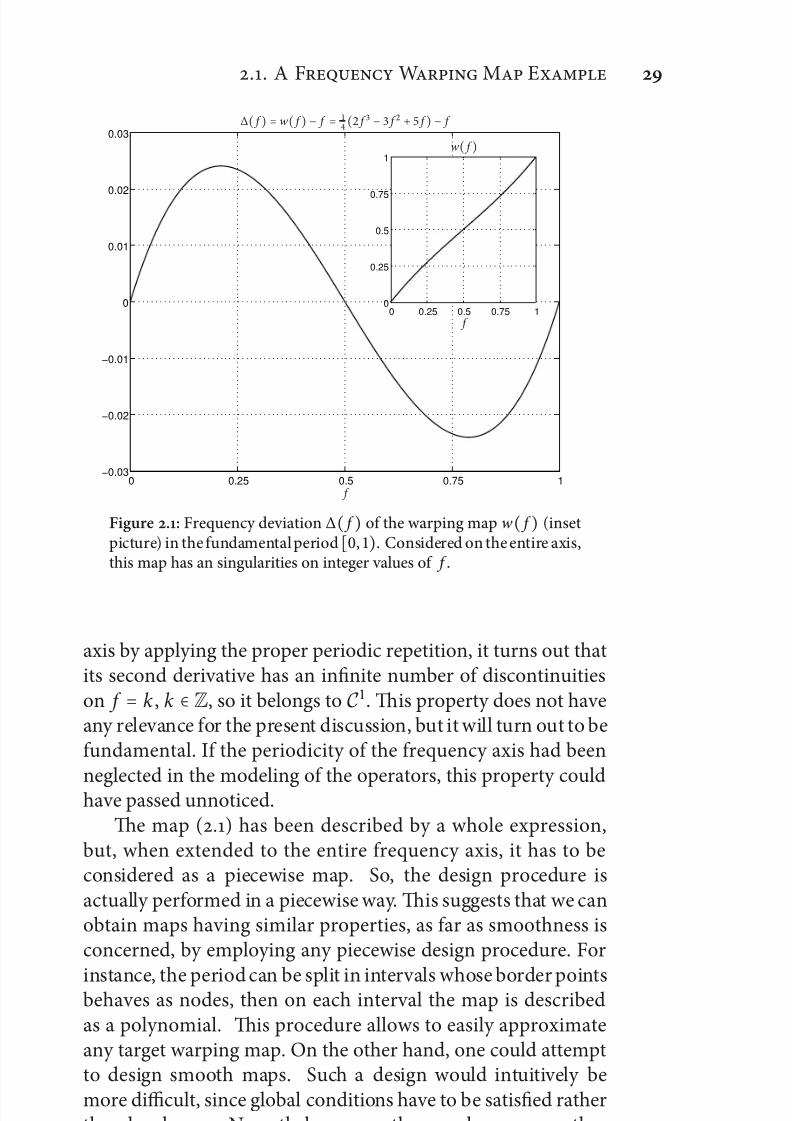
whose frequency deviation ∆( f ) = w( f ) − f has been depictedin Fig. .. e warping map w( f ) is represented in the insetpicture. As we said before, the frequency deviation can be
perceived in a better way, while the warping map may resultto be really close to the identity map w( f ) = f . Although thedeviation is really small, it affects the frequency warping matrixin a significant way, as it will be shown later, so the consideredexample can not be considered as a particular or pathologicalcase.
Warping map (.) has not been designed according to ap-plication requirements, it just has a demonstrative purpose and
will be used as a reference case in the rest of the work.For the moment, we can do some observations. If consideredonly on [, ), the function (.) would be smooth. In chapter we stressed on the fact that the frequency warping map hato be considered on the entire frequency axis, and we forcedthe representation of the presented operators in order to alwayshighlight the dependency by the deformation of the entire fre-quency axis. So, by extending (.) on the rest of the frequency
7/21/2019 Design and Computation of Warped Time-Frequency Transforms
http://slidepdf.com/reader/full/design-and-computation-of-warped-time-frequency-transforms 49/150
.. A F W M E
0 0.25 0.5 0.75 1−0.03
−0.02
−0.01
0
0.01
0.02
0.03∆( f ) = w( f ) − f =
( f − f + f ) − f
f
0 0.25 0.5 0.75 10
0.25
0.5
0.75
1
f
w( f )
Figure .: Frequency deviation ∆( f ) of the warping map w ( f ) (insetpicture) in the fundamentalperiod [, ). Considered on the entire axis,this map has an singularities on integer values of f .
axis by applying the proper periodic repetition, it turns out thatits second derivative has an infinite number of discontinuitieson f = k , k ∈ Z, so it belongs to C . is property does not haveany relevance for the present discussion, but it will turn out to befundamental. If the periodicity of the frequency axis had been
neglected in the modeling of the operators, this property couldhave passed unnoticed.e map (.) has been described by a whole expression,
but, when extended to the entire frequency axis, it has to beconsidered as a piecewise map. So, the design procedure isactually performed in a piecewise way. is suggests that we canobtain maps having similar properties, as far as smoothness isconcerned, by employing any piecewise design procedure. For
instance, the period can be split in intervals whose border pointsbehaves as nodes, then on each interval the map is describedas a polynomial. is procedure allows to easily approximateany target warping map. On the other hand, one could attemptto design smooth maps. Such a design would intuitively bemore difficult, since global conditions have to be satisfied ratherthan local ones. Nevertheless, smooth maps have some otheradvantages which will be shown later.

7/21/2019 Design and Computation of Warped Time-Frequency Transforms
http://slidepdf.com/reader/full/design-and-computation-of-warped-time-frequency-transforms 50/150
C . T F W M
. Sparsity of a Warping Matrix
Now we try to heuristically understand the operation behind
frequency warping. According to the way operator WFD wasdecomposed, a time-limited discrete sequence is first trans-formed in the frequency domain, then its spectrum is reshapedaccording to a warping function w and multiplied to an orthog-onalizing factor w ⁄ and finally transformed back in the time-domain. e factor w ⁄ , representing an amplitude modulation,i.e. a convolution in the time-domain, necessarily causes aduration enlargement, so that the original time-limited input
signal is potentially enlarged to the entire time-axis. is simpleconsideration explains the reason why it is not allowed to trun-cate the frequency warping matrix rows without compromisingthe unitary property.
Nevertheless, the amplitude modulation, acting in the samefashion on each column of WFD independently on n, does notcharacterize the structure of the warping matrix in a significantway. Instead, the reshaping of frequency axis carries major
effects. Since the spectrum is represented as a series of complexexponentials, the reshaping acts as a frequency modulation.Moreover, the modulating function is proportional to n, so thisaffects in a time-variant manner the warping matrix.
We remind that these considerations are intended to under-stand how to limit WFD HN to its rows indexed in a set Z M of M consecutive integers, according to the set ZN by with thecolumns have been limited. For clarity, we set:
ZN = nl , nl + , . . . , nr where n l stays for le and nr stays for right , and:
Z M = mt , md + , . . . , mbwhere mt stays for top and mb stays for bottom. e column axis,indexed by n, goes from le to right, while the row axis, indexedby m, goes from top to bottom. Given ZN , Z M must be chosen
so that only the significant entries of WFD HN are discarded.In order to evaluate an upper bound for mt and a lower
bound for mb we have to consider the line spectrum of the kernelof FWD , i.e. the line spectrum of an amplitude and frequency modulated set of periodic functions. By substituting w( f ) in thecomplex exponential by its linear approximation in f ∈ [, ):
w
( f
) ≃ w
( f
)+ w
( f
)⋅
( f − f
) = w
( f
) f + ρ

7/21/2019 Design and Computation of Warped Time-Frequency Transforms
http://slidepdf.com/reader/full/design-and-computation-of-warped-time-frequency-transforms 51/150
.. S W M
where ρn is an arbitrary phase contribution, it results:
FWD
( f , n
) ≃ w
( f
)e− jπn( w ( f ) f + ρ) f → f .
e effective carrier of the frequency modulation is representedby nw( f ). By neglecting the effects of the phase contributionand of the amplitude modulation, which causes only a further
n−constant duration enlargement, we get:
WFD(m, n, f ) ≃
e jπm f −n w ( f ) f d f
≃
e jπ (m−n w ( f )) f d f
≃ sinc(m − ⌈n w( f )⌉)where we deliberately made abuse of notation, since WFD couldnot depend on f and the sinc function stays for the Kroneckersymbol. Anyway, the result tells us how to determine thebounds of the interval where energy should be concentrated.
For minimizing and maximizing the position of the impulse⌈nw( f )⌉, we must distinguish three different cases for nl and
nr :
• nl < and nr < :
mt < −n l max w mb > −nr min w
• nl < and nr > :
mt < −n l max w mb > nr max w
• nl > and nr > :
mt < nl min w mb > nr max w.
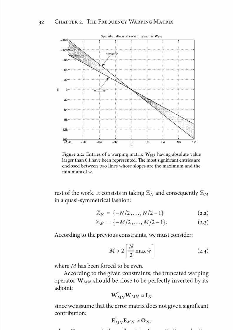
More generally, we can state that significant entries of W F Dare enclosed between two lines whose slopes are n max w andn min w. In Fig. ., the sparsity pattern of the warping operatorWFD relative to the warping function (.) has been represented.Since max w is equal to , for N = , the minimum re-quirement for the output length is M = . e influence of the minimum of the derivative is also shown. is figure alsorepresents a choice for ZN which will be commonly adopted in
7/21/2019 Design and Computation of Warped Time-Frequency Transforms
http://slidepdf.com/reader/full/design-and-computation-of-warped-time-frequency-transforms 52/150
C . T F W M
−128 −96 −64 −32 0 32 64 96 128
−160
−128
−96
−64
−32
0
32
64
96
128
160
Sparsity pattern of a warping matrix WFD
n
m
n max w
n min w
Figure .: Entries of a warping matrix WFD having absolute valuelarger than . have been represented. e most significant entries areenclosed between two lines whose slopes are the maximum and the
minimum of w .
rest of the work. It consists in taking ZN and consequently Z M
in a quasi-symmetrical fashion:
ZN = −N , . . . , N − (.)
Z M =
− M
, . . . , M
−
. (.)
According to the previous constraints, we must consider:
M > N
max w (.)
where M has been forced to be even.According to the given constraints, the truncated warping
operator W M N should be close to be perfectly inverted by its
adjoint:W†
M N W M N ≃ IN
since we assume that the error matrix does not give a significantcontribution:
E† M N E M N ≃ ON .
where ON represents the null matrix. A quantitative evaluationof the error will be treated in next chapters.
7/21/2019 Design and Computation of Warped Time-Frequency Transforms
http://slidepdf.com/reader/full/design-and-computation-of-warped-time-frequency-transforms 53/150
.. T-F S
. Time-Frequency Sampling
Now we want to describe frequency warping by its behavior in
time and frequency. More in details, we want to analyze the way the time-frequency representation of a signal is changed by thistransformation.
We remind that a time-frequency analysis is characterized by its basis vectors. e basis vectors of frequency warping, beingrepresented by a matrix, are given by the matrix rows. So, weshould study their time-frequency behavior in order to trace thecurves representing their paths on the time-frequency plane.
We point now that for the sparsity characterization we fo-cused on the matrix columns rather than on the matrix rows.To correctly perform this target change, we recall a generaleproperty of the unitary operators and a particular property of the warping operator.
e first property, which is reported in (.) for a genericunitary operator, particularized for frequency warping becomes:
WFD s = F†DWFDs = F
†D[F
†DW
†
]†
swhich means that s, a apart from FD
† on the le, is analyzedby means of unwarped complex exponential. Equivalently wecould have written:
WFD s = F†DWFD s = [W†FD]†[FDs].
which means that the spectrum of s is analyzed by means of unwarped complex exponential. In both representations, an
unwarping takes place instead of a warping, since operator Wis adjoint.
e second property consists in the possibility of represent-ing the adjoint warping operator, or rather the inverse one, by exploiting the inverse map w− :
W−(z , x ) = w−(z )δ (w−(z ) − y ).
Finally, it is clear that we must model the columns of WFDas we did for its rows provided that w is substituted by w− :
WFD†(n, m, f ) ≃
e jπnξ −m ˙w − ( f )ξ d ξ
≃
e jπ (n−m ˙w − ( f )) f d ξ
≃ sinc
(n − m w−
( f
))
7/21/2019 Design and Computation of Warped Time-Frequency Transforms
http://slidepdf.com/reader/full/design-and-computation-of-warped-time-frequency-transforms 54/150
C . T F W M
−8 −7 −6 −5 −4 −3 −2 −1 0 1 2 3 4 5 6 7 80
0.1
0.2
0.3
0.4
0.5
0.6
0.7
0.8
0.9
1
Time-frequency plane
n
f
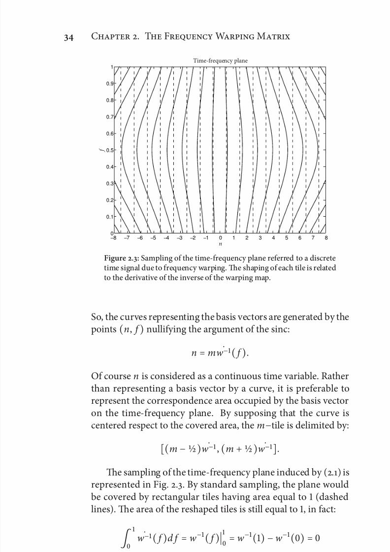
Figure .: Sampling of the time-frequency plane referred to a discretetime signal due to frequency warping. e shaping of each tile is relatedto the derivative of the inverse of the warping map.
So, the curves representing the basis vectors are generated by thepoints (n, f ) nullifying the argument of the sinc:
n = m w−( f ).
Of course n is considered as a continuous time variable. Rather
than representing a basis vector by a curve, it is preferable torepresent the correspondence area occupied by the basis vectoron the time-frequency plane. By supposing that the curve iscentered respect to the covered area, the m−tile is delimited by:
[(m − ⁄ ) w− , (m + ⁄ ) w−].
e sampling of the time-frequency plane induced by (.) is
represented in Fig. .. By standard sampling, the plane wouldbe covered by rectangular tiles having area equal to (dashedlines). e area of the reshaped tiles is still equal to , in fact:
w−( f )d f = w−( f )
= w−() −w−() =
since w− , being a warping map, has the same property as w.
7/21/2019 Design and Computation of Warped Time-Frequency Transforms
http://slidepdf.com/reader/full/design-and-computation-of-warped-time-frequency-transforms 55/150
.. S . -S M
. Smooth vs. non-Smooth Maps
Till now we just gave the schematic representation of a frequency
warping matrix. e analysis which brought to Fig. . was donein a qualitative manner, so we just got a rough binary descriptionin terms significant or not significant entry value. Here we wantto focus on the matrix coefficients decay.
Besides, we are interested in comparing the frequency warp-ing matrix WFD , or rather its truncation W M N , to its approxi-mated version W M N , which has been shown to be affected by time aliasing because of the sampling process performed in the
frequency domain. is aliasing effect has been modeled by analiasing operator A M N :
W MN = W MN +A M N .
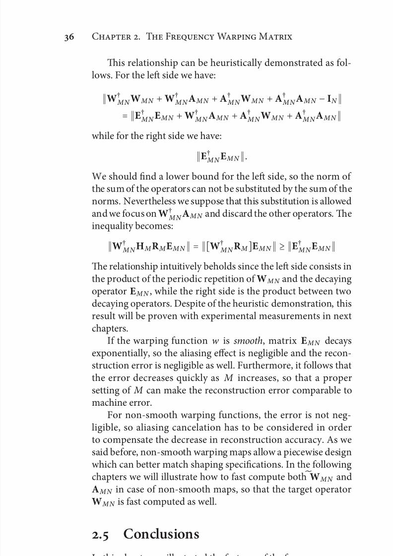
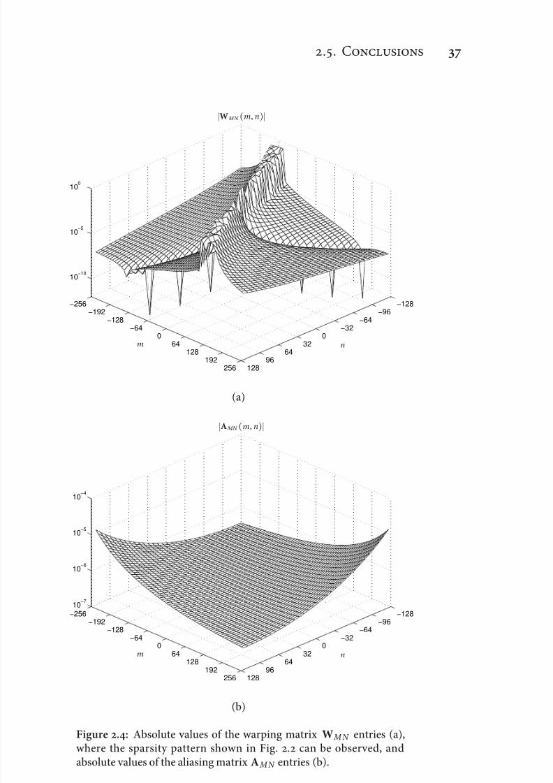
In Fig. . we represented the warping matrix W MN andthe aliasing matrix A M N referred to the warping map (.) for
N = and M = N . Since max w was shown to be
,
M , according to previously obtained constraints, is properly selected and guarantees that most of the frequency warpingmatrix energy has been enclosed in W M N .
By observing the decay of W M N coefficients over m, we inferthat the non truncated matrix WFD may have a slow decay.e relationship between the warping map properties and thedecay will be investigated later. Nevertheless, we notice that thediscarded coefficients of E M N produce a very regular aliasing
matrix. As a consequence, the aliasing operator A M N shouldhave a small rank, which means that it may be described by few basis vectors, or, equivalently, A MN may be computed in a fastmanner.
e reason why we are interested in efficiently computingA M N in order to compensate the difference between W M N andW M N is that aliasing causes a decrease in accuracy when theinverse warping is performed by the adjoint operator:
s − W† M N W MN s ≥ s −W†
M N W MN sthat is:
W† M N W MN − IN ≥ W†
MN W M N − IN .
where ⋅ represents the euclidian and the spectral norm for a vector and a matrix respectively.
7/21/2019 Design and Computation of Warped Time-Frequency Transforms
http://slidepdf.com/reader/full/design-and-computation-of-warped-time-frequency-transforms 56/150
C . T F W M
is relationship can be heuristically demonstrated as fol-lows. For the le side we have:
W† MN W M N +W† M N A M N +A† M N W M N +A† M N A M N − IN = E† MN E M N +W†
M N A M N +A† M N W M N +A†
M N A M N while for the right side we have:
E† M N E M N .
We should find a lower bound for the le side, so the norm of the sum of the operators can not be substituted by the sum of thenorms. Nevertheless we suppose that this substitution is allowedand we focus on W†
M N A M N and discard the other operators. einequality becomes:
W† M N H M R M E M N = [W†
M N R M ]E M N ≥ E† M N E M N
e relationship intuitively beholds since the le side consists inthe product of the periodic repetition of W M N and the decaying
operator E M N , while the right side is the product between twodecaying operators. Despite of the heuristic demonstration, thisresult will be proven with experimental measurements in nextchapters.
If the warping function w is smooth, matrix E M N decaysexponentially, so the aliasing effect is negligible and the recon-struction error is negligible as well. Furthermore, it follows thatthe error decreases quickly as M increases, so that a proper
setting of M can make the reconstruction error comparable tomachine error.
For non-smooth warping functions, the error is not neg-ligible, so aliasing cancelation has to be considered in orderto compensate the decrease in reconstruction accuracy. As wesaid before, non-smooth warping maps allow a piecewise designwhich can better match shaping specifications. In the followingchapters we will illustrate how to fast compute both
W M N and
A M N in case of non-smooth maps, so that the target operatorW M N is fast computed as well.
. Conclusions
In this chapter we illustrated the features of the frequency warp-ing matrix. We mainly focused on the role of the warping
7/21/2019 Design and Computation of Warped Time-Frequency Transforms
http://slidepdf.com/reader/full/design-and-computation-of-warped-time-frequency-transforms 57/150
.. C
−128−96
−64−32
032
6496
128
−256−192
−128−64
064
128192
256
10−10
10−5
100
W MN (m, n)
m n
(a)
−128−96
−64−32
032
6496
128
−256−192
−128−64
064
128192
256
10−7
10−6
10−5
10−4
A MN (m, n)
m n
(b)
Figure .: Absolute values of the warping matrix W M N entries (a),where the sparsity pattern shown in Fig. . can be observed, andabsolute values of the aliasing matrix A MN entries (b).
7/21/2019 Design and Computation of Warped Time-Frequency Transforms
http://slidepdf.com/reader/full/design-and-computation-of-warped-time-frequency-transforms 58/150
C . T F W M
map in determining the time-duration characteristics and theway the time-frequency plane is sampled. In this framework,we were able to detect the constraints for correctly truncating
the warping matrix and to illustrate the connection betweenrequired time-frequency specifications and warping map de-sign. Moreover, we showed how the map smoothness can affectthe importance of aliasing in the computation of the frequency warping operator.

7/21/2019 Design and Computation of Warped Time-Frequency Transforms
http://slidepdf.com/reader/full/design-and-computation-of-warped-time-frequency-transforms 59/150

7/21/2019 Design and Computation of Warped Time-Frequency Transforms
http://slidepdf.com/reader/full/design-and-computation-of-warped-time-frequency-transforms 60/150
7/21/2019 Design and Computation of Warped Time-Frequency Transforms
http://slidepdf.com/reader/full/design-and-computation-of-warped-time-frequency-transforms 61/150
P
IIAlgorithms for
Frequency Warping

7/21/2019 Design and Computation of Warped Time-Frequency Transforms
http://slidepdf.com/reader/full/design-and-computation-of-warped-time-frequency-transforms 62/150
7/21/2019 Design and Computation of Warped Time-Frequency Transforms
http://slidepdf.com/reader/full/design-and-computation-of-warped-time-frequency-transforms 63/150
C
Nonuniform Fast
Fourier Transform
T first part of this work was dedicated to present and settle
the warping transforms we are dealing with. Starting fromthe continuous case, we redefined Fourier and warping opera-tors in case of discrete-time axis. e discrete-time frequency warping was identified as the target operator to be modeled forthe achievement of a feasible implementation. At this aim, twomajor problems were detected, consisting in the computation of a continuous integral and non-finite dimensions of the resultingoperator. is last issue was solved by properly truncating thewarping matrix, while the first one was overcome by decom-posing the operator in two additive terms, one representingthe frequency sampled discrete frequency warping operator andthe other one representing time aliasing occurring because of the sampling in frequency. Moreover, the frequency sampledoperator was described as the composition of a nonuniformand scaled discrete Fourier transform and an inverse ordinary discrete Fourier transform. Fast algorithms for the discreteFourier transform are widely known, while algorithms for thenonuniform one deserve a deep insight.
Here we first recall some algorithms which have been pre-sented in literature, then we introduce an original contribu-tion [] which will be shown to be optimum in case of densesampling of the frequency axis (output length larger then inputlength), as it occurs for frequency warping.
7/21/2019 Design and Computation of Warped Time-Frequency Transforms
http://slidepdf.com/reader/full/design-and-computation-of-warped-time-frequency-transforms 64/150
C . N F T
. Introduction to NUFFT
e Discrete Fourier Transform (DFT) is known to be a fun-
damental transformation in most fields of signal processing.It is very efficiently computed since algorithms which yieldsO(N log N ) rather than O(N ) operations have been found.However, many applications are based on the computation of Fourier coefficients of nonuniformly sampled frequencies. isoccurs when frequency warping techniques are introduced []or when directional analysis techniques are applied on two di-mensional signals, like the polar Fourier Transform, the RadonTransform and the Contourlet Transform []. In such casesthe transformation is referred as Nonuniform Fourier Trans-form and its fast implementation as Nonuniform Fast FourierTransform (NUFFT).
In previous works [, , ] NUFFT is implemented by means of interpolation, i.e. each nonuniform Fourier coefficientis obtained by interpolating the Discrete Fourier coefficientsin the neighborhood of the considered nonuniform frequency.In order to improve the performances, an oversampled DFTis employed, where the oversampling factor is generally takenequal to . Moreover, the input signal is previously scaled by asuitable scaling vector. In [], the interpolator is obtained by aleast square approximation with respect to the oversampled DFTbasis. A significant improvement is obtained in [], where firsta bell-shaped interpolator is chosen and then the scaling vector
is obtained by imposing a minimization on the approximationerror. Finally in [], scaling is considered as if it were applied tothe oversampled DFT basis, although it is actually applied on theinput signal. en a least square interpolator is computed. eoptimization of the scaling vector is an untractable problem andso it is chosen according to [], resulting in a slight performanceimprovement.
Here we introduce a different approach. Each nonuniform
Fourier exponential in the interval between two contiguousuniform Fourier frequencies is approximated by a small set of orthogonal vectors, obtained by a singular value decomposition(SVD). Only a single set of orthogonal vectors is needed. Infacts, every nonuniform Fourier exponential can be obtainedby modulating a nonuniform Fourier exponential of a singleinterval. So, first the input signal is scaled according to a smallset of vectors. Second, the scaled versions of the input signal are
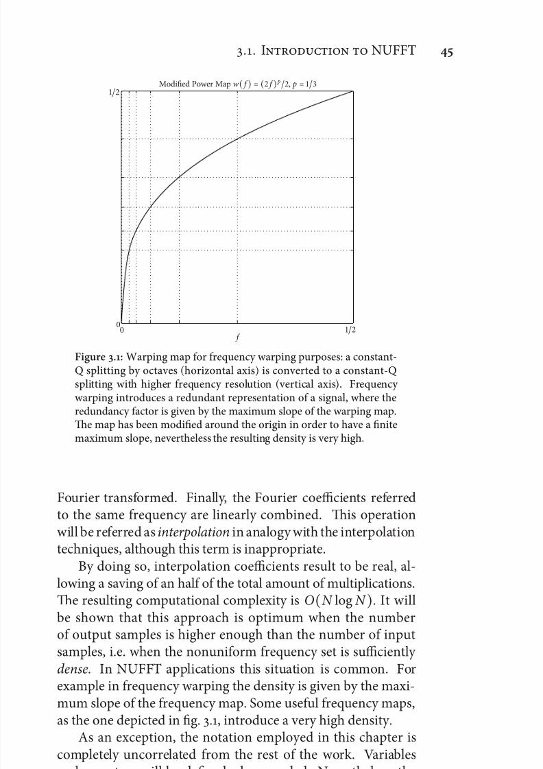
7/21/2019 Design and Computation of Warped Time-Frequency Transforms
http://slidepdf.com/reader/full/design-and-computation-of-warped-time-frequency-transforms 65/150
.. I NUFFT
Modified Power Map w( f ) = ( f ) p, p =
f
Figure .: Warping map for frequency warping purposes: a constant-Q splitting by octaves (horizontal axis) is converted to a constant-Qsplitting with higher frequency resolution (vertical axis). Frequency warping introduces a redundant representation of a signal, where theredundancy factor is given by the maximum slope of the warping map.e map has been modified around the origin in order to have a finitemaximum slope, nevertheless the resulting density is very high.
Fourier transformed. Finally, the Fourier coefficients referredto the same frequency are linearly combined. is operation
will be referred as interpolation in analogy with the interpolationtechniques, although this term is inappropriate.By doing so, interpolation coefficients result to be real, al-
lowing a saving of an half of the total amount of multiplications.e resulting computational complexity is O(N log N ). It willbe shown that this approach is optimum when the numberof output samples is higher enough than the number of inputsamples, i.e. when the nonuniform frequency set is sufficiently
dense. In NUFFT applications this situation is common. Forexample in frequency warping the density is given by the maxi-mum slope of the frequency map. Some useful frequency maps,as the one depicted in fig. ., introduce a very high density.
As an exception, the notation employed in this chapter iscompletely uncorrelated from the rest of the work. Variablesand operators will be defined when needed. Nevertheless, thedescription of the proposed algorithm will take advantage of the
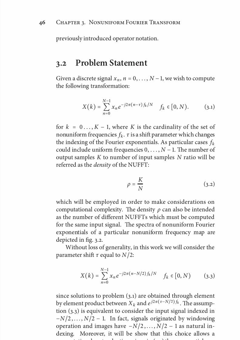
7/21/2019 Design and Computation of Warped Time-Frequency Transforms
http://slidepdf.com/reader/full/design-and-computation-of-warped-time-frequency-transforms 66/150
C . N F T
previously introduced operator notation.
. Problem Statement
Given a discrete signal x n , n = , . . . , N − , we wish to computethe following transformation:
X (k) = N −
n=
x n e− jπ (n−τ ) f k N f k ∈ [, N ). (.)
for k = . . . , K − , where K is the cardinality of the set of nonuniform frequencies f k . τ is a shi parameter which changesthe indexing of the Fourier exponentials. As particular cases f kcould include uniform frequencies , . . . , N − . e number of output samples K to number of input samples N ratio will bereferred as the density of the NUFFT:
ρ = K N
(.)
which will be employed in order to make considerations oncomputational complexity. e density ρ can also be intendedas the number of different NUFFTs which must be computedfor the same input signal. e spectra of nonuniform Fourierexponentials of a particular nonuniform frequency map are
depicted in fig. ..Without loss of generality, in this work we will consider the
parameter shi τ equal to N :
X (k) = N −
n=
x n e− jπ (n−N ) f k N f k ∈ [, N ) (.)
since solutions to problem (.) are obtained through elementby element product between X k and e jπ (τ −N ) f k . e assump-tion (.) is equivalent to consider the input signal indexed in−N , . . . , N − . In fact, signals originated by windowingoperation and images have −N , . . . , N − as natural in-dexing. Moreover, it will be show that this choice allows acomputational cost reduction, since in (.) the exponentials arenearly symmetric respect to n = N
.

7/21/2019 Design and Computation of Warped Time-Frequency Transforms
http://slidepdf.com/reader/full/design-and-computation-of-warped-time-frequency-transforms 67/150
.. I A
47
36
24
12
0 0
12
24
36
47
10−3
10−2
10−1
100
Spectra of nonuniform Fourier exponentials.
f k n
Figure .: Spectra of nonuniform Fourier exponentials. Nonuniformfrequencies f k , k = , . . . , K − , are obtained by uniformly samplinga nonlinear function such that f = and f K = . Spectra decay slowly since periodic repetition of a nonuniform Fourier exponential
have discontinuities.
. Interpolation Approach
e interpolation approach is based on the on the calculation of an oversampled FFT Y of the input signal scaled by a suitable vector c n :
Y i = N −n=
cn x n e− jπni M i = , . . . , M − (.)
where M = mN and m ∈ N is the oversampling factor. Generally m is taken equal to , since taking m > does not increase per-formances significantly. en, the frequency axis is consideredas a collection of M intervals [i − M , i), i = , . . . , M − ,and nonuniform Fourier exponentials of the i-th interval are
approximated by linearly combining L FFT coefficients in theneighborhood of Y i :
X ( f k) = L−
l =−L
Y i+l ϕ( f km − (i + l )) f k ∈ [i − m, i). (.)
is formulation is valid for even values of L, but can be easily extended to odd values.
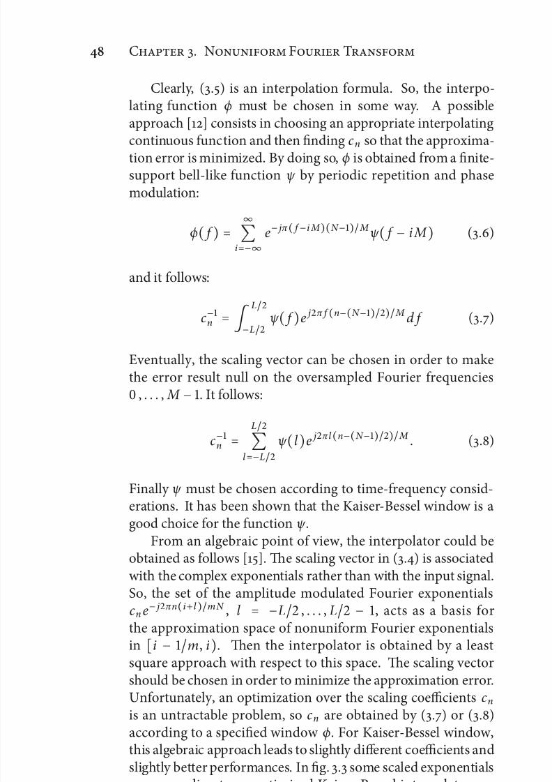
7/21/2019 Design and Computation of Warped Time-Frequency Transforms
http://slidepdf.com/reader/full/design-and-computation-of-warped-time-frequency-transforms 68/150
C . N F T
Clearly, (.) is an interpolation formula. So, the interpo-lating function ϕ must be chosen in some way. A possibleapproach [] consists in choosing an appropriate interpolating
continuous function and then finding cn so that the approxima-tion error is minimized. By doing so, ϕ is obtained from a finite-support bell-like function ψ by periodic repetition and phasemodulation:
ϕ( f ) = ∞
i=−∞
e− jπ ( f −i M )(N −) M ψ ( f − iM ) (.)
and it follows:
c−n =
L
−Lψ ( f )e jπ f (n−(N −)) M d f (.)
Eventually, the scaling vector can be chosen in order to makethe error result null on the oversampled Fourier frequencies , . . . , M − . It follows:
c−n =
L
l =−L
ψ (l )e jπl (n−(N −)) M . (.)
Finally ψ must be chosen according to time-frequency consid-erations. It has been shown that the Kaiser-Bessel window is agood choice for the function ψ .
From an algebraic point of view, the interpolator could beobtained as follows []. e scaling vector in (.) is associatedwith the complex exponentials rather than with the input signal.So, the set of the amplitude modulated Fourier exponentialscn e− jπn(i+l )mN , l = −L , . . . , L − , acts as a basis forthe approximation space of nonuniform Fourier exponentialsin [i − m, i). en the interpolator is obtained by a leastsquare approach with respect to this space. e scaling vector
should be chosen in order to minimize the approximation error.Unfortunately, an optimization over the scaling coefficients cn
is an untractable problem, so cn are obtained by (.) or (.)according to a specified window ϕ. For Kaiser-Bessel window,this algebraic approach leads to slightly different coefficients andslightly better performances. In fig. . some scaled exponentialscorresponding to an optimized Kaiser-Bessel interpolator arerepresented.
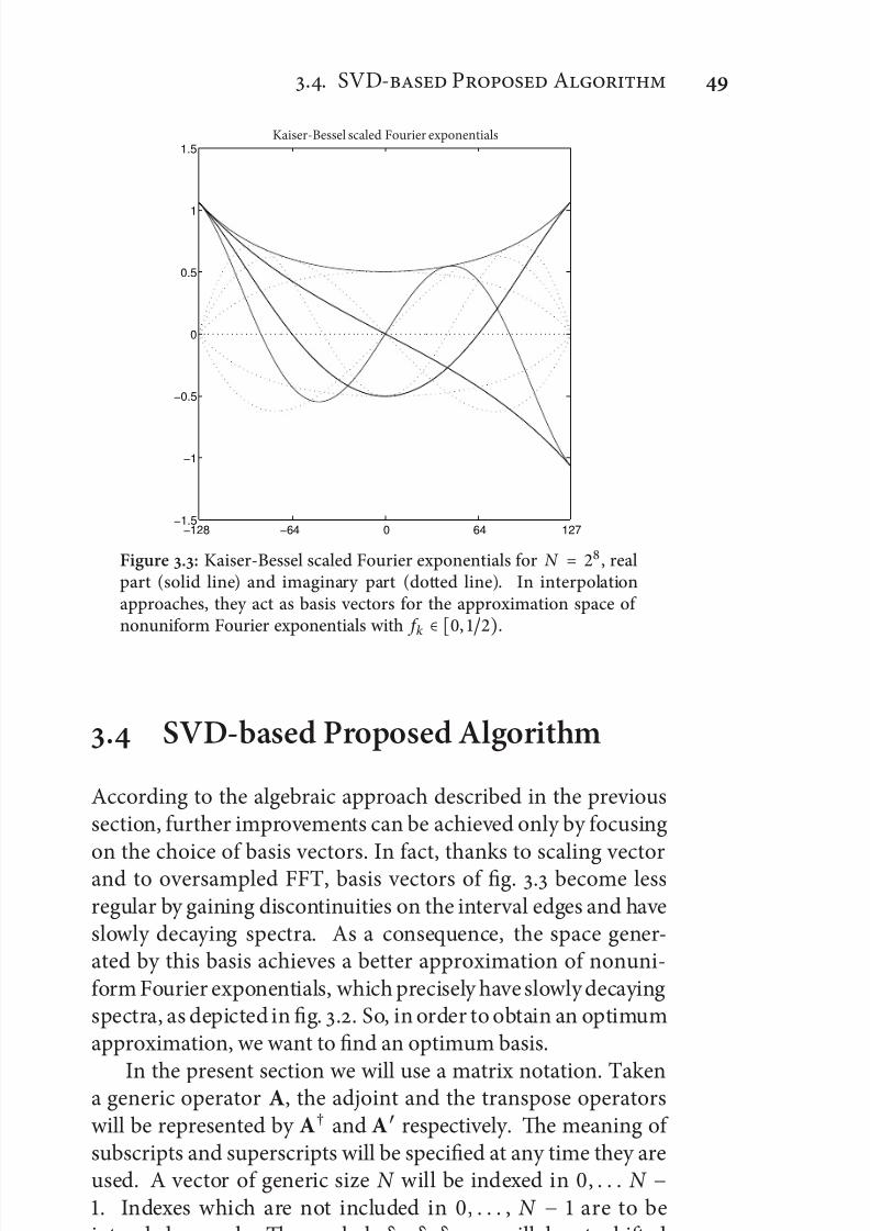
7/21/2019 Design and Computation of Warped Time-Frequency Transforms
http://slidepdf.com/reader/full/design-and-computation-of-warped-time-frequency-transforms 69/150
.. SVD- P A
−128 −64 0 64 127−1.5
−1
−0.5
0
0.5
1
1.5Kaiser-Bessel scaled Fourier exponentials
Figure .: Kaiser-Bessel scaled Fourier exponentials for N = , realpart (solid line) and imaginary part (dotted line). In interpolationapproaches, they act as basis vectors for the approximation space of nonuniform Fourier exponentials with f k ∈ [, ).
. SVD-based Proposed Algorithm
According to the algebraic approach described in the previoussection, further improvements can be achieved only by focusing
on the choice of basis vectors. In fact, thanks to scaling vectorand to oversampled FFT, basis vectors of fig. . become lessregular by gaining discontinuities on the interval edges and haveslowly decaying spectra. As a consequence, the space gener-ated by this basis achieves a better approximation of nonuni-form Fourier exponentials, which precisely have slowly decayingspectra, as depicted in fig. .. So, in order to obtain an optimumapproximation, we want to find an optimum basis.
In the present section we will use a matrix notation. Takena generic operator A, the adjoint and the transpose operatorswill be represented by A† and A′ respectively. e meaning of subscripts and superscripts will be specified at any time they areused. A vector of generic size N will be indexed in , . . . N −. Indexes which are not included in , . . . , N − are to beintended as modN . e symbols δ , δ δ , . . ., will denote shiedimpulsive column vectors of suitable size.
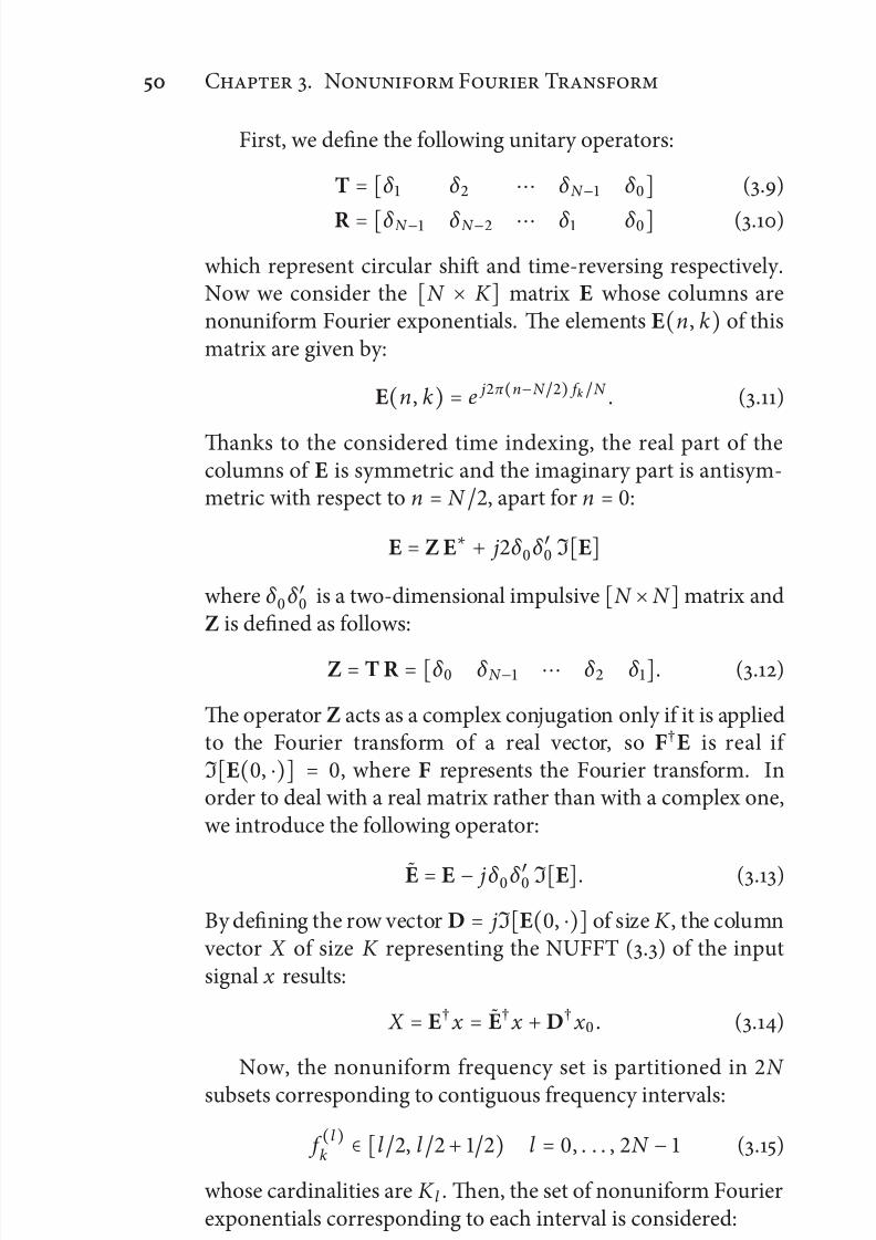
7/21/2019 Design and Computation of Warped Time-Frequency Transforms
http://slidepdf.com/reader/full/design-and-computation-of-warped-time-frequency-transforms 70/150
C . N F T
First, we define the following unitary operators:
T =
[δ δ ⋯ δ N − δ
] (.)
R = [δ N − δ N − ⋯ δ δ ] (.)
which represent circular shi and time-reversing respectively.Now we consider the [N × K ] matrix E whose columns arenonuniform Fourier exponentials. e elements E(n, k) of thismatrix are given by:
E
(n, k
) = e jπ (n−N ) f k N . (.)
anks to the considered time indexing, the real part of thecolumns of E is symmetric and the imaginary part is antisym-metric with respect to n = N , apart for n = :
E = Z E∗+ jδ δ ′ I[E]
where δ δ ′ is a two-dimensional impulsive [N ×N ]matrix and
Z is defined as follows:
Z = T R = [δ δ N − ⋯ δ δ ]. (.)
e operator Z acts as a complex conjugation only if it is appliedto the Fourier transform of a real vector, so F†E is real if I[E(, ⋅)] = , where F represents the Fourier transform. Inorder to deal with a real matrix rather than with a complex one,we introduce the following operator:
E = E − jδ δ ′ I[E]. (.)
By defining the row vector D = jI[E(, ⋅)] of size K , the column vector X of size K representing the NUFFT (.) of the inputsignal x results:
X = E† x = E†x +D† x . (.)
Now, the nonuniform frequency set is partitioned in N subsets corresponding to contiguous frequency intervals:
f (l )k ∈ [l , l + ) l = , . . . , N − (.)
whose cardinalities are K l . en, the set of nonuniform Fourierexponentials corresponding to each interval is considered:
El
(n, k
) = e jπ (n−N ) f
(l )
k N (.)

7/21/2019 Design and Computation of Warped Time-Frequency Transforms
http://slidepdf.com/reader/full/design-and-computation-of-warped-time-frequency-transforms 71/150
.. SVD- P A
0
0.125
0.25
.375
0.5 0
64
128
192
255
−1
−0.5
0
0.5
1
Inverse Fourier Transforms of nonuniform Fourier exponentials
f k n
Figure .: Entries of the matrix F†E . When nonuniform frequency f ktends to , the matrix column tends to be an impulse. e columns are
very correlated, so the rank of the matrix is small.
It is worth to note that El , for even l , could be obtained by modulating the column vectors of a nonuniform Fourier matrixreferred to a suitable set of frequencies f k ∈ [, ), which willbe represented as El , . For odd l , El could be obtained in thesame way from a nonuniform Fourier matrix whose frequenciesrefer to f k ∈
[−
,
), which could be also obtained by con-
jugating a suitable matrix E l , . Modulation can be converted incircular shi by passing in the Fourier domain, so, by some somecalculations, it follows:
El = (−)i F T−i F†El , l = i (.)
El = (−)i F T−i F†E∗l , R l = i − . (.)
where the formulation (.) has been exploited in order to deal
with the real matrixes F† ˜
El , . In general, each matrix ˜El , refersto randomly distributed frequencies in [, ). In order to find
a single basis for the column vectors of all matrixes El , , wecan equally consider a generic matrix E which ideally has ascolumn vectors every possible nonuniform Fourier exponentialsin [, ). In practice, it suffices to consider a finite set of nonuniform frequencies which densely cover the whole [, )interval. is matrix has very correlated column vectors, as

7/21/2019 Design and Computation of Warped Time-Frequency Transforms
http://slidepdf.com/reader/full/design-and-computation-of-warped-time-frequency-transforms 72/150
C . N F T
depicted in fig. ., so its rank results to be small for a certainprecision. As a consequence, a singular value decompositioncan be introduced, i.e. F†E = U S V′. e singular values
decay exponentially, so we could consider a reduced number Lof singular values and neglect the others:
F†E ≃ ULSLV′L (.)
where UL and VL are constituted by the first L columns of Uand V respectively and SL is a square matrix constituted by the first L rows and columns of S. e column vectors of UL
represent an optimum basis for all the matrixes E, l . en, thedecomposition is extended to El in the following way:
El ≃ F T−i ULP′l l = i (.)
El ≃ F T−i Z UL P′l l = i − (.)
where each P l is a real [K l × L] matrix which linearly combinethe column vectors of UL in order to obtain the best approxi-
mation of ˜El , . Since UL has orthogonal columns, P l are simply obtained by computing:
Pl = (Ti F†El )′UL l = i (.)
Pl = (Z Ti F†El )′UL l = i − . (.)
e column vectors of each El are approximated by linearly combining the columns of F T−i UL or F T−i Z UL through the
rows of the matrix Pl . In order to compute (.), we mustcalculate the scalar products between x and the columns of F T−i UL and F T−i Z UL in an efficient way. With some algebra,it has been found that first, x must be scaled by the Fourierantitrasformed vectors of UL , W = F†UL :
X = diag(x )W (.)
where diag
(x
) is a matrix having x as main diagonal. e
columns of W corresponding to the first singular values aredepicted in fig. .. en, the Fourier transforms of the column vectors of X produce the needed N × L scalar products:
Q = F X (.)
Each row of Q will be pointed by Qi . Finally we obtain that˜ X (l ) = E†
l x is given by the product between a
[K l × L
] matrix
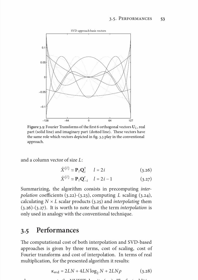
7/21/2019 Design and Computation of Warped Time-Frequency Transforms
http://slidepdf.com/reader/full/design-and-computation-of-warped-time-frequency-transforms 73/150
.. P
−128 −64 0 64 127
−0.1
−0.05
0
0.05
0.1
SVD-approach basis vectors
Figure .: Fourier Transforms of the first orthogonal vectors UL , realpart (solid line) and imaginary part (dotted line). ese vectors havethe same role which vectors depicted in fig. . play in the conventionalapproach.
and a column vector of size L:
˜ X (l ) ≃ P l Q†i l = i (.)
˜ X (l ) ≃ P l Q′−i l = i − (.)
Summarizing, the algorithm consists in precomputing inter-
polation coefficients (.)-(.), computing L scaling (.),calculating N × L scalar products (.) and interpolating them(.)-(.). It is worth to note that the term interpolation isonly used in analogy with the conventional technique.
. Performances
e computational cost of both interpolation and SVD-basedapproaches is given by three terms, cost of scaling, cost of Fourier transforms and cost of interpolation. In terms of realmultiplication, for the presented algorithm it results:
κsvd = LN + LN log N + LN ρ (.)
where ρ represents the NUFFT density (.). e first additiveterm derives from (.), where L element-by-element products

7/21/2019 Design and Computation of Warped Time-Frequency Transforms
http://slidepdf.com/reader/full/design-and-computation-of-warped-time-frequency-transforms 74/150
C . N F T
between a real and a complex vector of size N are computed, i.e.LN real multiplications. e second term derives from (.),where L Fourier transforms of vectors of size N are computed.
Each Fourier transform needs N log N real multiplications.Finally, the third term derives from (.)-(.) where K = ρ N scalar products between a real and a complex vector of size Lare computed, or, equally, L complex scaling of a real vector of size ρN . e cost of D† x (.) can be neglected. roughanalogous considerations, for interpolation techniques it results:
κint = N + N log N + LN ρλ. (.)
e factor λ > is an effective parameter which takes intoaccount that, for the same value of L, SVD-based approach hasbetter performances, as depicted in fig. .. For useful values of L, λ is nearly equal to , . As far as memory requirements areconcerned, in terms of real numbers for the SVD-approach itresults:
µsvd = LN + LN ρ + N ρ (.)
where terms correspond to the complex vectors W to the realinterpolation coefficients Pl and to the vector D respectively.Only LN real coefficients are necessary for the vectors W, sincethey are the Fourier transforms of the real vectors UL . Similarly,for interpolation approach it results:
µint = N + LN ρλ. (.)
A fair comparison between the two approaches is quite hard.Sufficient conditions for SVD-approach to be less expensive thaninterpolation approach are:
ρ > log N ⇒ κsvd < κint (.)
ρ > ⇒ µsvd < µint (.)
In worst cases, when ρ ≈ , the proposed method would consistin more multiplications because of the computation of L Fouriertransforms. Nevertheless, the algorithm has a serial structure,since each basis vector requires the computation of a scaling, afast Fourier transform and its contribution to the interpolation,which is actually another scaling. Moreover, it does not involvecomplex multiplications in the scaling and interpolation compu-tation. Furthermore, since the algorithm is based on orthogonal
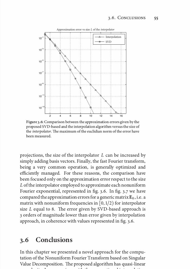
7/21/2019 Design and Computation of Warped Time-Frequency Transforms
http://slidepdf.com/reader/full/design-and-computation-of-warped-time-frequency-transforms 75/150
.. C
2 4 6 8 10 12 14 16
10−13
10−11
10−9
10−7
10−5
10−3
10−1
Approximation error vs size L of the interpolator
Interpolation
SVD
Figure .: Comparison between the approximation errors given by theproposed SVD-based and the interpolation algorithm versus the size of the interpolator . e maximum of the euclidian norm of the error havebeen measured.
projections, the size of the interpolator L can be increased by simply adding basis vectors. Finally, the fast Fourier transform,being a very common operation, is generally optimized andefficiently managed. For these reasons, the comparison havebeen focused only on the approximation error respect to the sizeL of the interpolator employed to approximate each nonuniformFourier exponential, represented in fig. .. In fig. . we havecompared the approximation errors for a generic matrix E , i.e. amatrix with nonuniform frequencies in [, ) for interpolatorsize L equal to . e error given by SVD-based approach is orders of magnitude lower than error given by interpolationapproach, in coherence with values represented in fig. ..
. Conclusions
In this chapter we presented a novel approach for the compu-tation of the Nonuniform Fourier Transform based on SingularValue Decomposition. e proposed algorithm has quasi-linearcomplexity. In comparison with the conventional interpolationapproach, our proposed approach has been shown to have a
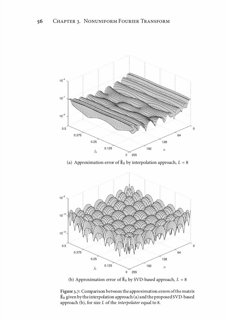
7/21/2019 Design and Computation of Warped Time-Frequency Transforms
http://slidepdf.com/reader/full/design-and-computation-of-warped-time-frequency-transforms 76/150
C . N F T
0
0.125
0.25
0.375
0.5 0
64
128
192
255
10−9
10−7
10−5
f kn
(a) Approximation error of E by interpolation approach, L =
0
0.125
0.25
0.375
0.5 0
64
128
192
255
10−12
10−10
10−8
f k n
(b) Approximation error of ˜E by SVD-based approach, L
=
Figure .: Comparison between the approximation errors of the matrixE given by theinterpolation approach (a)and theproposedSVD-basedapproach (b), for size L of the interpolator equal to .

7/21/2019 Design and Computation of Warped Time-Frequency Transforms
http://slidepdf.com/reader/full/design-and-computation-of-warped-time-frequency-transforms 77/150
.. C
higher computational cost for the calculation of the projectioncomponents, but a lower cost for interpolating them. Moreover,this algorithm provides advantages in terms of computational
structure, being based on Fast Fourier Transforms and realmultiplications.

7/21/2019 Design and Computation of Warped Time-Frequency Transforms
http://slidepdf.com/reader/full/design-and-computation-of-warped-time-frequency-transforms 78/150
7/21/2019 Design and Computation of Warped Time-Frequency Transforms
http://slidepdf.com/reader/full/design-and-computation-of-warped-time-frequency-transforms 79/150
C
Factorization of the
Aliasing Matrix
T present chapter is the core of the entire work. In fact,
the issues which are going to be treated occupy a major rel-evance in terms of importance originality and innovation of theobtained results. Basically, the content of this chapter completesthe analytical characterization of the frequency warping matrixin order to make a fast computation achievable. Although itconfigures as a completion, it involves a lot of mathematicalmodeling effort and carries many implications on the natureof the operator under consideration which goes beyond simplecomputational issues. From the following analysis, as well as afactorization for the aliasing matrix which is necessary to cor-rectly describe the frequency warping operator by compensatingthe effects of having sampled the frequency axis, useful hints forthe warping map design strategy are also obtained. Moreover,the present model acts a starting point for further investigations,like the quantitative characterization of reconstruction accuracy,which is treated in the next chapter.
e results which are illustrated here are a detailed explana-tion of some previously obtained preliminaries results [, ].
e notation is consistent with the one described in chapter ,although some letters will be reassigned to other operators forfulfill representation necessities.

7/21/2019 Design and Computation of Warped Time-Frequency Transforms
http://slidepdf.com/reader/full/design-and-computation-of-warped-time-frequency-transforms 80/150
C . F A
. Problem Statement and Methodology
e purpose of this chapter is to model the operator A M N
involved, together with W M N , in the computation of operatorW M N , as they were introduced in chapter . e investigation islimited to the case of non-smooth maps only, since it has beenpreviously shown that the usefulness of aliasing compensationis not significant in case of smooth maps. e interest in non-smooth maps is based on the ease in designing suitable warpingmaps.
e aim of this investigation is to achieve the ability of compute the aliasing operator by means of the warping mapfeatures only, without explicitly calculate the difference betweenW M N and W M N . Moreover, it would be desirable to obtain afast algorithm for computing the output of A M N with a linearcomplexity.
e methodology can be briefly described as follows. Weexploit the fact that aliasing is equivalently obtained as theperiodic repetition along columns of operator E M N . When M is properly set, E M N has a regular behavior since it mainly depends on the singularities of the warping map only. In fact,singularities consisting in steps in the frequency domain, i.e. fast variations, can be equivalently described in the time domain by considering large time indexes, like in matrix E M N , which willbe also referred as tails matrix, since it contains the discardedtails of WF D . So, aer having determined a model for E M N , a
model for A M N can be easily obtained as well.As far as the fast computation is concerned, since the modelfor A MN turns out to be a factorization like a singular valuedecomposition with a fast decaying internal kernel, a linearcomplexity is easily obtained by properly truncating the kernel.Moreover, the kernel is the only factor sensibly depending on thecharacteristics of the warping map, so the obtained algorithm is very efficient and allows a simple computational architecture.
Before going through the mathematical modeling, which isfull of complex demonstrations, we propose a heuristic approachto the problem. is constitutes an attempt to trace out the pathwhich inspired the further deep mathematical insight, in orderto present it just as formalization of some simple intuitions.
To get some further simplifications in notation, here weneglect the subscript M N on operators W M N , E M N and A M N .is would generate an ambiguity between W, representing
7/21/2019 Design and Computation of Warped Time-Frequency Transforms
http://slidepdf.com/reader/full/design-and-computation-of-warped-time-frequency-transforms 81/150
.. H M T M
the native axis warping, and W M N , representing the frequency warping. Antway the first one is not needed here. Letters S, Dand U, introduced in chapter , are reassigned to new operators.
. Heuristic Model of the Tails Matrix
Before describing the mathematical modeling of the aliasingmatrix, let us make some heuristic considerations about thewarping matrix decay.
As a case study, we still consider the non–smooth warping
map w in (.). As we observed before, w ∈ C
, max w = and there is only one singularity placed in f = within thefundamental interval [, ). In Fig. . we plotted some columnsof the warping matrix in a wide temporal range in both semilog(Fig. .(a)) and loglog axis (Fig. .(b)). Independently on n,each column converges to the same asymptote. In loglog axis,for w ∈ C , the asymptote is given by a line whose slope is −(see Section ..).
Now we suppose to be able to determine the intercept of the asymptote in Fig. .(b). We can imagine to subtract theasymptote and define a residual matrix G. Some of its columnshave been depicted in Fig. .(a). e decay is shown to be pro-portional to lines having slope equal to − but having differentintercepts. Again, we can subtract the asymptotes and obtain anew matrix which will be referred as G and shown in Fig. .(b)for some columns. In general, we define:
Gl (m, n) = WFD(m, n) − l
i=
ζ i ,nm−i
( M )−i
where the generic subscript l means that asymptotes from m−
till m−l have been subtracted and the normalization to M has been introduced in order to obtain well-scaled values forcoefficients ζ i ,n . is process could be iterated for l → ∞.
However, as it will be demonstrated in Section .., aer someiterations, matrix Gl converges to in (Z∖Z M )×ZN , whereZN
and Z M are settled according to the quasi-symmetrical choice(.)-(.). is means that the columns of E(m, n) canberepre-sented as a linear combination of m−i when the coefficients ζ i ,n
are known. en, when periodic repetition can be analytically computed, aliasing can be represented as a linear combinationof analytically known vectors.
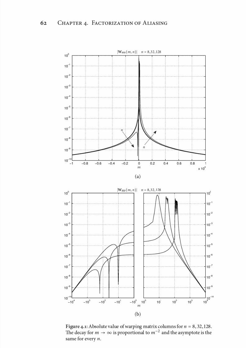
7/21/2019 Design and Computation of Warped Time-Frequency Transforms
http://slidepdf.com/reader/full/design-and-computation-of-warped-time-frequency-transforms 82/150
C . F A
−1 −0.8 −0.6 −0.4 −0.2 0 0.2 0.4 0.6 0.8 1
x 104
10−10
10−9
10−8
10−7
10−6
10−5
10−4
10−3
10−2
10−1
100
n
n
WFD(m, n) n = ,,
m
(a)
−104
−103
−102
−101
−100
10−10
10−9
10−8
10−7
10−6
10−5
10−4
10−3
10−2
10−1
100
100
101
102
103
10410
−10
10−9
10−8
10−7
10−6
10−5
10−4
10−3
10−2
10−1
100
WFD(m, n) n = ,,
m
(b)
Figure .: Absolute value of warping matrix columns for n = , , .e decay for m →∞ is proportional to m− and the asymptote is thesame for every n.
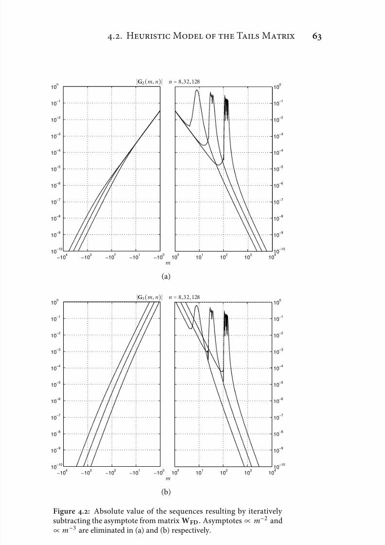
7/21/2019 Design and Computation of Warped Time-Frequency Transforms
http://slidepdf.com/reader/full/design-and-computation-of-warped-time-frequency-transforms 83/150
.. H M T M
−104
−103
−102
−101
−100
10−10
10−9
10−8
10−7
10−6
10−5
10−4
10−3
10−2
10−1
100
100
101
102
103
10410
−10
10−9
10−8
10−7
10−6
10−5
10−4
10−3
10−2
10−1
100
G(m, n) n = ,,
m
(a)
−104
−103
−102
−101
−100
10−10
10−9
10−8
10−7
10−6
10−5
10−4
10−3
10−2
10−1
100
100
101
102
103
10410
−10
10−9
10−8
10−7
10−6
10−5
10−4
10−3
10−2
10−1
100
G(m, n) n = ,,
m
(b)
Figure .: Absolute value of the sequences resulting by iteratively subtracting the asymptote from matrix WFD . Asymptotes ∝ m− and∝ m− are eliminated in (a) and (b) respectively.
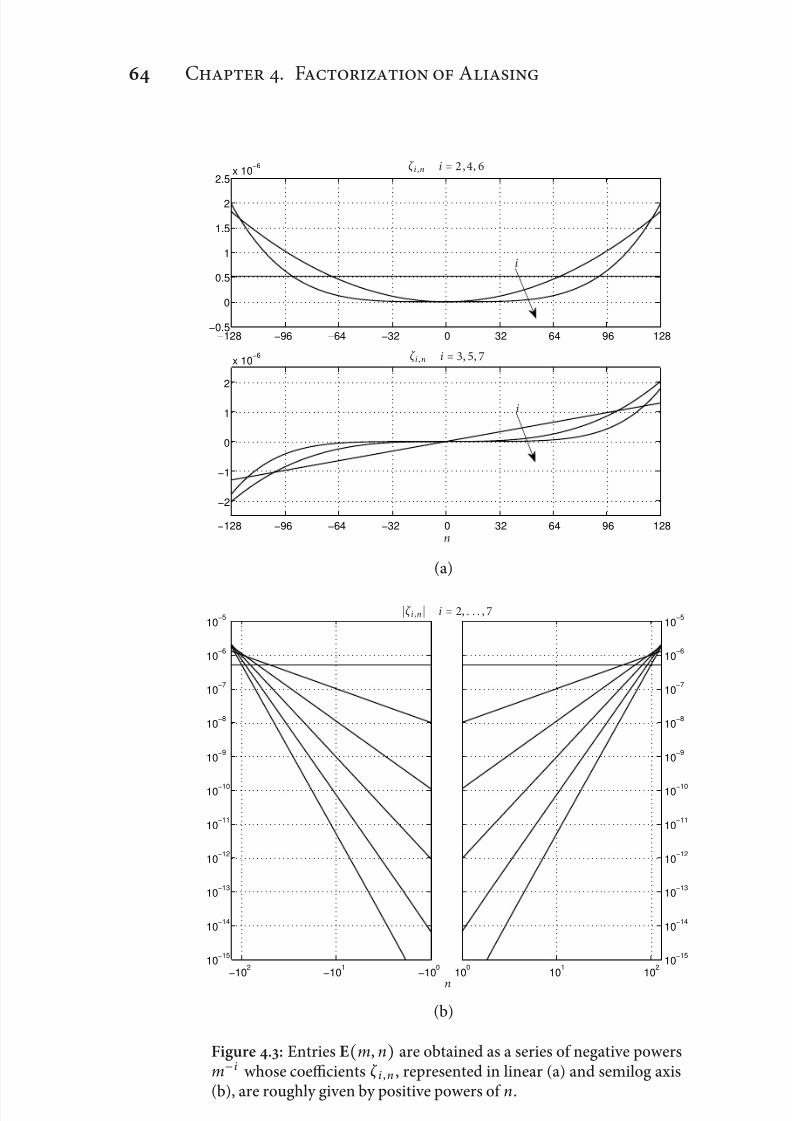
7/21/2019 Design and Computation of Warped Time-Frequency Transforms
http://slidepdf.com/reader/full/design-and-computation-of-warped-time-frequency-transforms 84/150
C . F A
−128 −96 −64 −32 0 32 64 96 128−0.5
0
0.5
1
1.5
2
2.5x 10
−6
−128 −96 −64 −32 0 32 64 96 128
−2
−1
0
1
2
x 10−6
i
i
ζ i ,n i = ,,
ζ i ,n i = , ,
n
(a)
−102
−101
−100
10−15
10−14
10−13
10−12
10−11
10−10
10−9
10−8
10−7
10−6
10−5
100
101
102
10−15
10−14
10−13
10−12
10−11
10−10
10−9
10−8
10−7
10−6
10−5
ζ i ,n i = , . . . ,
n
(b)
Figure .: Entries E(m, n) are obtained as a series of negative powersm−i whose coefficients ζ i ,n , represented in linear (a) and semilog axis(b), are roughly given by positive powers of n.
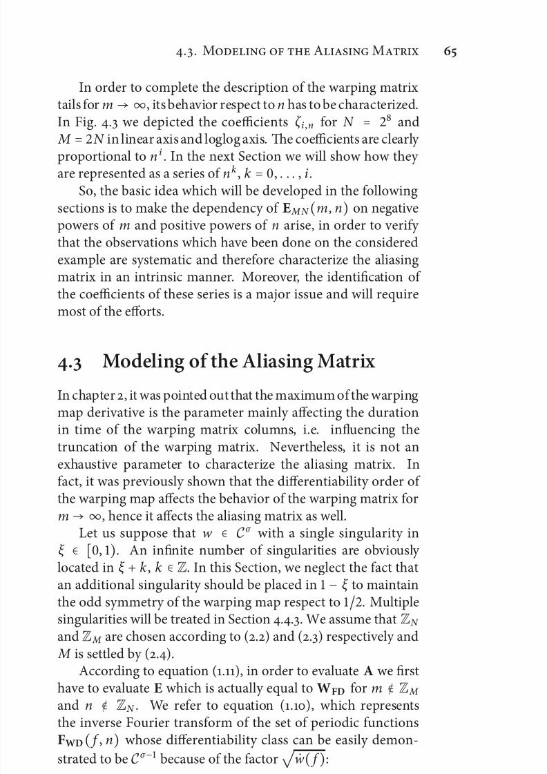
7/21/2019 Design and Computation of Warped Time-Frequency Transforms
http://slidepdf.com/reader/full/design-and-computation-of-warped-time-frequency-transforms 85/150
.. M A M
In order to complete the description of the warping matrixtails for m → ∞, its behavior respect to n has to be characterized.In Fig. . we depicted the coefficients ζ i ,n for N = and
M = N in linear axis and loglog axis. e coefficients are clearly proportional to n i . In the next Section we will show how they are represented as a series of nk , k = , . . . , i.
So, the basic idea which will be developed in the followingsections is to make the dependency of E M N (m, n) on negativepowers of m and positive powers of n arise, in order to verify that the observations which have been done on the consideredexample are systematic and therefore characterize the aliasingmatrix in an intrinsic manner. Moreover, the identification of the coefficients of these series is a major issue and will requiremost of the efforts.
. Modeling of the Aliasing Matrix
In chapter , it was pointed out that the maximum of the warping
map derivative is the parameter mainly affecting the durationin time of the warping matrix columns, i.e. influencing thetruncation of the warping matrix. Nevertheless, it is not anexhaustive parameter to characterize the aliasing matrix. Infact, it was previously shown that the differentiability order of the warping map affects the behavior of the warping matrix for
m → ∞, hence it affects the aliasing matrix as well.Let us suppose that w
∈ Cσ with a single singularity in
ξ ∈ [, ). An infinite number of singularities are obviously located in ξ + k , k ∈ Z. In this Section, we neglect the fact thatan additional singularity should be placed in − ξ to maintainthe odd symmetry of the warping map respect to . Multiplesingularities will be treated in Section ... We assume that ZN
and Z M are chosen according to (.) and (.) respectively and
M is settled by (.).
According to equation (.), in order to evaluate A we firsthave to evaluate E which is actually equal to WFD for m ∉ Z M
and n ∉ ZN . We refer to equation (.), which representsthe inverse Fourier transform of the set of periodic functionsFWD( f , n) whose differentiability class can be easily demon-
strated to be Cσ − because of the factor
w( f ):
w ∈
Cσ ⇒ FWD ∈
Cσ − . (.)
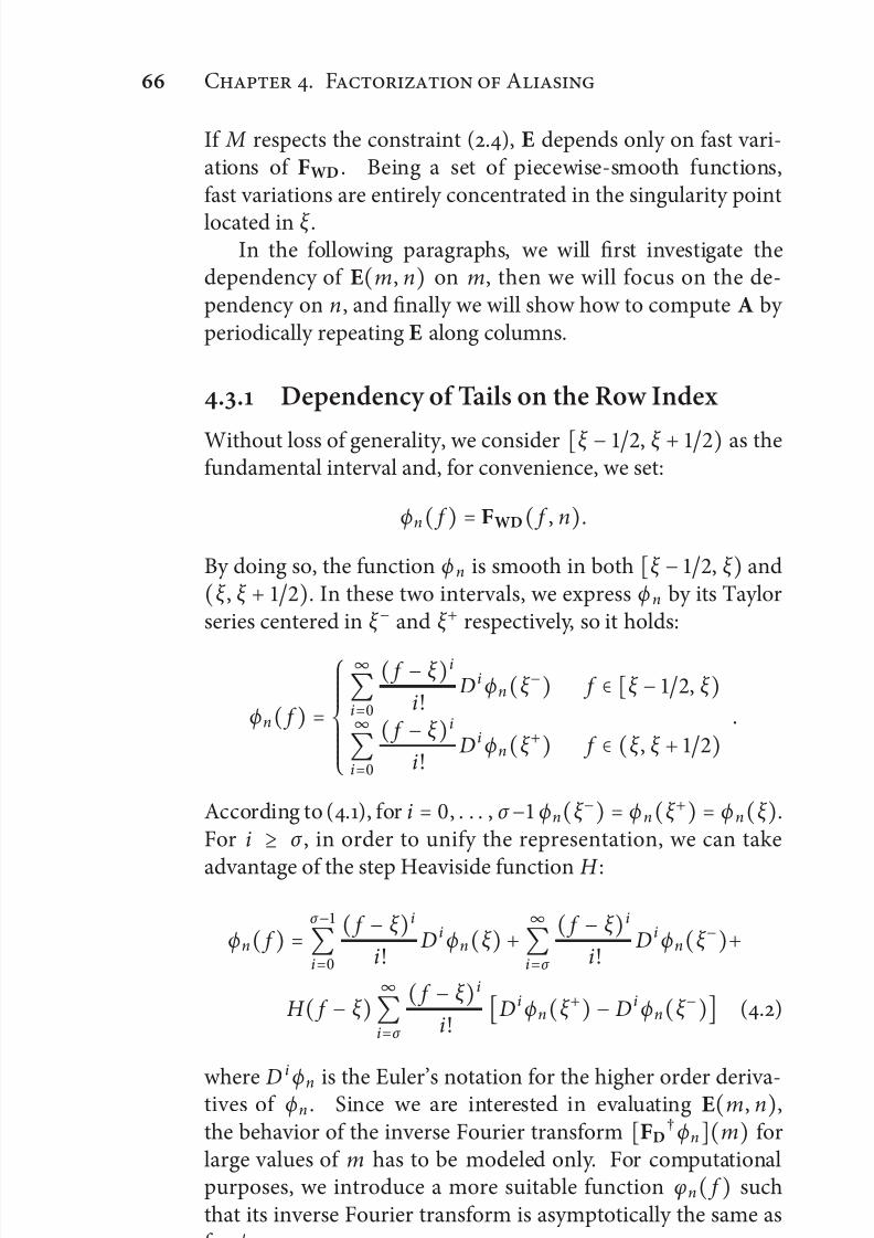
7/21/2019 Design and Computation of Warped Time-Frequency Transforms
http://slidepdf.com/reader/full/design-and-computation-of-warped-time-frequency-transforms 86/150
C . F A
If M respects the constraint (.), E depends only on fast vari-ations of FWD . Being a set of piecewise-smooth functions,fast variations are entirely concentrated in the singularity point
located in ξ .In the following paragraphs, we will first investigate the
dependency of E(m, n) on m, then we will focus on the de-pendency on n, and finally we will show how to compute A by periodically repeating E along columns.
.. Dependency of Tails on the Row Index
Without loss of generality, we consider [ξ − , ξ + ) as thefundamental interval and, for convenience, we set:
ϕn( f ) = FWD( f , n).
By doing so, the function ϕ n is smooth in both [ξ − , ξ ) and(ξ , ξ + ). In these two intervals, we express ϕ n by its Taylorseries centered in ξ − and ξ + respectively, so it holds:
ϕn( f ) =⎧⎪⎪⎪⎪⎪⎪⎨⎪⎪⎪⎪⎪⎪⎩
∞
i=
( f − ξ )i
i!D i ϕn(ξ −) f ∈ [ξ − , ξ )
∞
i=
( f − ξ )i
i!D i ϕn(ξ +) f ∈ (ξ , ξ + ) .
According to (.), for i = , . . . , σ − ϕn(ξ −) = ϕn(ξ +) = ϕn(ξ ).For i ≥ σ , in order to unify the representation, we can take
advantage of the step Heaviside function H :
ϕn( f ) = σ −
i=
( f − ξ )i
i! D i ϕn(ξ ) + ∞
i=σ
( f − ξ )i
i! D i ϕn(ξ −)+
H ( f − ξ ) ∞i=σ
( f − ξ )i
i!D i ϕn(ξ +) − D i ϕn(ξ −) (.)
where Di
ϕn is the Euler’s notation for the higher order deriva-tives of ϕn . Since we are interested in evaluating E(m, n),the behavior of the inverse Fourier transform [FD
† ϕn](m) forlarge values of m has to be modeled only. For computationalpurposes, we introduce a more suitable function φn( f ) suchthat its inverse Fourier transform is asymptotically the same asfor ϕn :
[FD
† φn
](m
) =
[FD
†ϕn
](m
) m ∉ Z M .
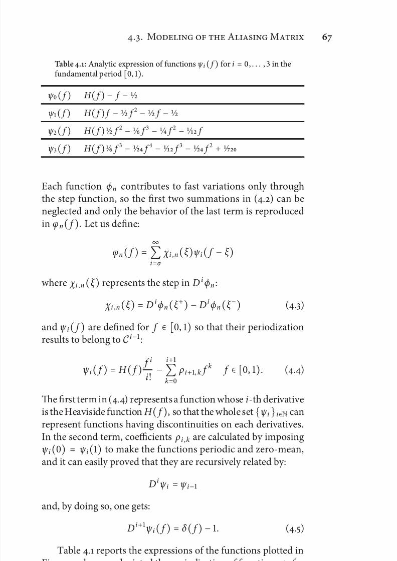
7/21/2019 Design and Computation of Warped Time-Frequency Transforms
http://slidepdf.com/reader/full/design-and-computation-of-warped-time-frequency-transforms 87/150
.. M A M
Table .: Analytic expression of functions ψ i( f ) for i = , . . . , in thefundamental period [, ).
ψ ( f ) H ( f ) − f − ⁄ ψ ( f ) H ( f ) f − ⁄ f − ⁄ f − ⁄
ψ ( f ) H ( f ) ⁄ f − ⁄ f − ⁄ f − ⁄ f
ψ ( f ) H ( f ) ⁄ f − ⁄ f − ⁄ f − ⁄ f + ⁄
Each function ϕn contributes to fast variations only through
the step function, so the first two summations in (.) can beneglected and only the behavior of the last term is reproducedin φn( f ). Let us define:
φn( f ) = ∞
i=σ
χ i ,n(ξ )ψ i( f − ξ )where χ i ,n
(ξ
) represents the step in D i ϕn :
χ i ,n(ξ ) = D i ϕn(ξ +) − D i ϕn(ξ −) (.)
and ψ i( f ) are defined for f ∈ [, ) so that their periodizationresults to belong to C i−:
ψ i( f ) = H ( f ) f i
i! −
i+
k=
ρi+, k f k f ∈ [, ). (.)
e first term in (.) represents a function whose i-th derivativeis the Heaviside function H ( f ), so that the whole setψ ii∈N canrepresent functions having discontinuities on each derivatives.In the second term, coefficients ρi ,k are calculated by imposingψ i() = ψ i() to make the functions periodic and zero-mean,and it can easily proved that they are recursively related by:
D iψ i
= ψ i−
and, by doing so, one gets:
D i+ψ i( f ) = δ ( f ) − . (.)
Table . reports the expressions of the functions plotted inFig. ., where we depicted the periodization of functions ψ i fori = , . . . , in the interval
[−,
]. As i increases, the presence
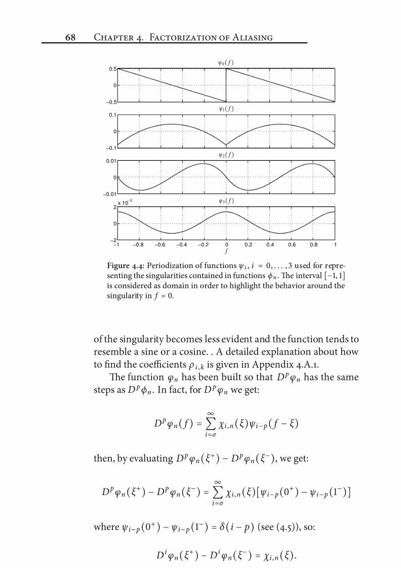
7/21/2019 Design and Computation of Warped Time-Frequency Transforms
http://slidepdf.com/reader/full/design-and-computation-of-warped-time-frequency-transforms 88/150
C . F A
−0.5
0
0.5
−0.1
0
0.1
−0.01
0
0.01
−1 −0.8 −0.6 −0.4 −0.2 0 0.2 0.4 0.6 0.8 1−2
0
2x 10
−3
ψ ( f )
ψ ( f )
ψ ( f )
ψ ( f )
f
Figure .: Periodization of functions ψ i , i = , . . . , used for repre-senting the singularities contained in functions ϕn . e interval [−, ]is considered as domain in order to highlight the behavior around the
singularity in f =
.
of the singularity becomes less evident and the function tends toresemble a sine or a cosine. . A detailed explanation about how to find the coefficients ρ i ,k is given in Appendix .A..
e function φn has been built so that D pφn has the samesteps as D pϕn . In fact, for D pφn we get:
D pφn( f ) = ∞
i=σ
χ i ,n(ξ )ψ i− p( f − ξ )then, by evaluating D pφn(ξ +) − D pφn(ξ −), we get:
D
p
φn(ξ
+
)−
D
p
φn(ξ
−
) = ∞
i=σ χ i ,n(ξ )[ψ i− p(+
)−
ψ i− p(−
)]where ψ i− p(+) − ψ i− p(−) = δ (i − p) (see (.)), so:
D i φn(ξ +) − D i φn(ξ −) = χ i ,n(ξ ).
e behavior of E
(m, n
)can be inferred by studying FD
† φn ,
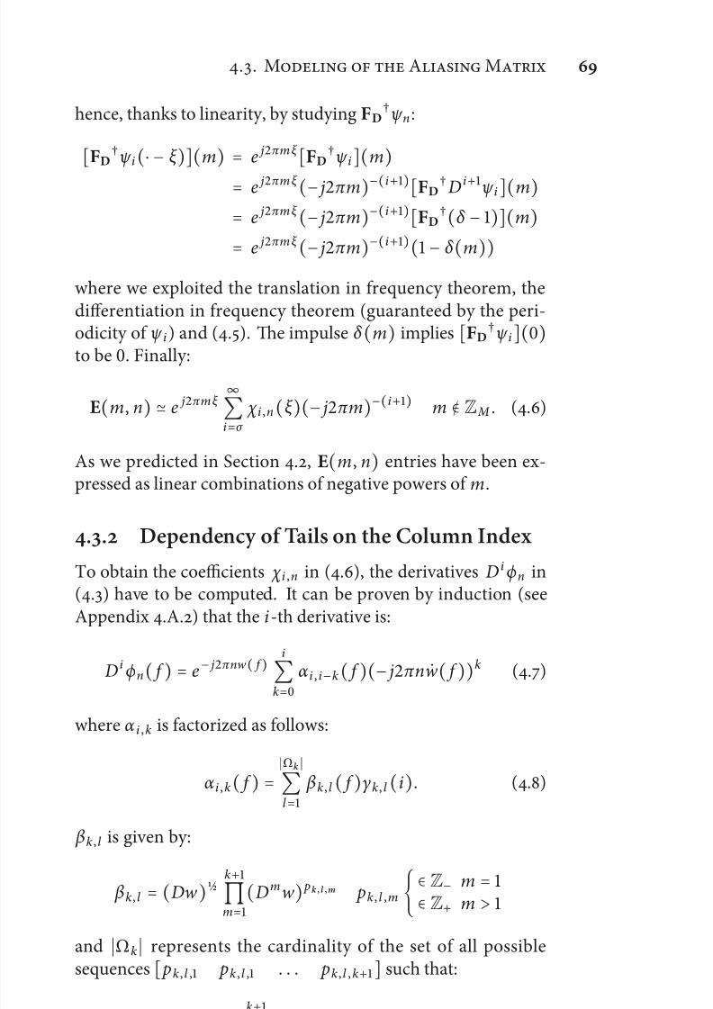
7/21/2019 Design and Computation of Warped Time-Frequency Transforms
http://slidepdf.com/reader/full/design-and-computation-of-warped-time-frequency-transforms 89/150
.. M A M
hence, thanks to linearity, by studying FD†ψ n :
[FD
†ψ i
(⋅ − ξ
)](m
) = e jπm ξ
[FD
†ψ i
](m
)= e jπm ξ (− jπ m)−(i+)[FD† D i+ψ i](m)
= e jπm ξ (− jπ m)−(i+)[FD†(δ − )](m)
= e jπm ξ (− jπ m)−(i+)( − δ (m))where we exploited the translation in frequency theorem, thedifferentiation in frequency theorem (guaranteed by the peri-odicity of ψ i ) and (.). e impulse δ
(m
) implies
[FD
†ψ i
](
)to be . Finally:
E(m, n) ≃ e jπmξ ∞
i=σ
χ i ,n(ξ )(− jπ m)−(i+) m ∉ Z M . (.)
As we predicted in Section ., E(m, n) entries have been ex-pressed as linear combinations of negative powers of m.
.. Dependency of Tails on the Column Index
To obtain the coefficients χ i ,n in (.), the derivatives D i ϕn in(.) have to be computed. It can be proven by induction (seeAppendix .A.) that the i-th derivative is:
D i ϕn( f ) = e− jπnw ( f )i
k=
αi , i−k( f )(− jπ n w( f ))k (.)
where α i ,k is factorized as follows:
αi ,k( f ) = Ωk
l =
βk , l ( f )γk, l (i). (.)
βk , l is given by:
βk, l = (Dw)⁄k+
m=(Dmw) pk , l ,m pk , l ,m ∈ Z− m = ∈ Z+ m >
and Ωk represents the cardinality of the set of all possiblesequences [ pk , l , pk , l , . . . pk , l ,k+] such that:
k+
m=
pk , l ,m ⋅ m = k . (.)
7/21/2019 Design and Computation of Warped Time-Frequency Transforms
http://slidepdf.com/reader/full/design-and-computation-of-warped-time-frequency-transforms 90/150
C . F A
A formal demonstration of these statements is reported in Ap-pendix .A.. In Table . we gave closed expressions of βk , l andγk , l for k = , . . . , . As a convention, βk , is defined as the only
function among β k, l containing the k + degree derivative:
βk , = (Dw)−⁄ Dk+w. (.)
With the above positions, according to (.), we have:
• for σ = coefficients χ i ,n are given by D i ϕn(ξ +) −D i ϕn(ξ −). In the resulting summation, factors e− jπnw (ξ )
and
(− jπ n
) can be extracted.
χ i ,n(ξ ) = e− jπnw (ξ )i
k=
(− jπ n)k
(αi , i−k(ξ +)(w(ξ +))k− αi , i−k(ξ −)(w(ξ −))k). (.)
• for σ > we can exploit the factorization (.):
χ i ,n(ξ ) = e− jπnw (ξ )i−σ
k=(− jπ nw(ξ ))k
Ωk
l =
( βi−k , l (ξ +) − βi−k , l (ξ −))γi−k , l (i). (.)
In (.) the summation over k has been considered from to i − σ rather than from to i since the function containing
the maximum derivative degree βi−k , = (Dw)−⁄
Di−k+
w iscontinue for k > i − σ .
It is worth to note that, according to (.) and (.), whenσ > all the information about the warping map, apart fromw(ξ ) and w(ξ ) is enclosed in β k , l . is means that most of thealgorithm structure does not depend on the particular shape of the warping maps.
.. Periodic Repetition of Tails
Now equation (.) can be applied to obtain an expression forA. Since coefficients χ i ,n do not depend on m, the summationin (.) is applied directly on m−(i+)e jπm ξ :
k≠
e jπ (m−k M )ξ
(m − kM
)i+ = e jπm ξ
k≠
e− jπ k M ξ
(m − kM
)i+

7/21/2019 Design and Computation of Warped Time-Frequency Transforms
http://slidepdf.com/reader/full/design-and-computation-of-warped-time-frequency-transforms 91/150
.. M A M
Table .: Expressions of βk , l and γk , l for k = , . . . .
k, l βk , l γk , l (i)
, (Dw)⁄
, (Dw)−⁄ Dw ⁄ i
, (Dw)−⁄ Dw ⁄ (i − i + i)
, (Dw)−⁄ (Dw) ⁄ (i − i + i − i)
, (Dw)−⁄ Dw ⁄ (i − i + i − i)
, (Dw)
−⁄
D
wD
w
⁄
(i
− i
+ i
− i
+ i), (Dw)−⁄ (Dw)
⁄ (i − i + i − i + i − i)
and if the following condition is satisfied:
M ξ ∈ N (.)
then e− jπ k M ξ = , k ∈ Z and the term e jπ (m−k M )ξ can befactored out. Equation (.) simply means that the singularity must be placed on one of the M points on which the frequency axis is sampled for the computation of W M ,N . It is not arestrictive hypothesis, but it has to be taken into account whenthe warping map is designed. Moreover, since:
(z − k)−(i+) = (−
)i
i! D
i
z
z − k
ζ (z ) = π cot(π z )−
z =
k≠
z − k z ≤
therefore:
k≠
(m − kM )i+ = (−
)i
M i+
i!
D i ζ
(m
M
).
Finally A can be represented by:
A(m, n) ≃ e jπm ξ ∞
i=σ
χ i ,n(ξ )(−)i
i!
(− jπ )i+
M i+ D i ζ (m M ).
(.)which completely describes the analytical modeling of aliasing.

7/21/2019 Design and Computation of Warped Time-Frequency Transforms
http://slidepdf.com/reader/full/design-and-computation-of-warped-time-frequency-transforms 92/150
C . F A
. Fast Warping Transforms
In the present Section we deal with the problem of compactly
calculating the analytical description which has been previously introduced. Moreover, we cope with the problem of performingthe multiplication to the matrix A in a fast way, since, accordingto equation (.), a summation of infinite terms is still needed.Furthermore, in case ξ ∈ (, ), we will take into account thesymmetrical singularity placed in−ξ which is needed for the oddsymmetry of the warping map.
.. Matrix Representation of Aliasing
e results summarized in equations (.), (.) and (.),(.) can be arranged in a compact and efficient matrix repre-sentation. e coefficients χ i ,n , apart from the complex expo-nential and other factors involving w, can be seen as differencebetween the products of a row vector having α i , i−k as entries anda column vector having the powers of n as entries. At this aim,
we first introduce a matrix K whose generic entry is:
K(i , k) = α i , i−k k ≤ i otherwise
i , k = , , . . .
en, three different contributions are considered: V, N, D. efirst matrix contains all the powers of n normalized to N so that its entries turn out to be nearly independent on the
dimension of the problem:
V(k , n) = nk
(N )k n ∈ ZN , k = , , . . .
e other (diagonal) matrixes are introduced to compensate thisnormalization and account for the powers of − jπ w:
N
= diag
[(− jπ N
)k
] k
= , , . . .
D = diag[wk] k = , , . . .
and have to be multiplied on the le of V. By doing so, thedependance of coefficients χ on ξ , apart from the complexexponential factor, is entirely enclosed in matrixes K and D,which, when evaluated in ξ + and ξ −, will be referred as Kξ + andDξ + , Kξ − and Dξ − respectively. As for (.) and (.), the case
7/21/2019 Design and Computation of Warped Time-Frequency Transforms
http://slidepdf.com/reader/full/design-and-computation-of-warped-time-frequency-transforms 93/150
.. F W T
σ > is only a particular case of the case σ = where can referto a single matrix Dξ since w(ξ −) = w(ξ +). So, we have:
• for σ = :X = Kξ +Dξ + −Kξ −Dξ −
• for σ > :X = [Kξ + −Kξ −]Dξ .
We point out that the first σ lower diagonals of X starting fromthe main diagonal are null. Finally we define:
Q = diag[e− jπnw (ξ )] n ∈ ZN
so that χ i ,n can be calculated as XNVQ. It is worth to pointout that the input is indexed in ZN according to the choice wepreviously made on the input signal (.).
Once χ i ,n is computed, equation (.) has to be consideredfor the computation of E and equation (.) for the computationof A. As far as E is concerned, we define:
Y(m, i) = ⎧⎪⎪⎪⎨⎪⎪⎪⎩m−(i+)
( M )−(i+) m ∉ Z M
otherwise
i = , , . . .
together with the following diagonal matrixes to be multipliedon the right and on the le of Y respectively:
M
= diag
[(− jπ M
)−(i+)
] i
= , , . . .
P = diag[e jπmξ ] m ∈ Zso that for E we get the compact expression:
E = PYMXNVQ.
In a similar way, for the operator A we define:
U(m, i) = (−)i
i+ i! D i ζ (m M ) m ∈ Z M , i = , , . . .
so that it results:A = PUMXNVQ (.)
where P has to be restricted to Z M and the output is clearly indexed in Z M as well. In Fig. . some columns of matrix U
for M = have been depicted.
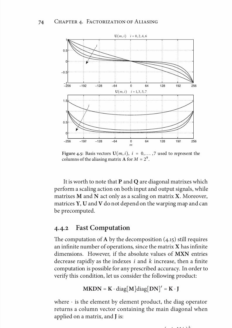
7/21/2019 Design and Computation of Warped Time-Frequency Transforms
http://slidepdf.com/reader/full/design-and-computation-of-warped-time-frequency-transforms 94/150
C . F A
−256 −192 −128 −64 0 64 128 192 256−1
−0.5
0
0.5
1
−256 −192 −128 −64 0 64 128 192 256
0
0.5
1
1.5
U(m, i) i = , ,,
U(m, i) i = , , ,
m
i
i
Figure .: Basis vectors U(m, i), i = , . . . , used to represent thecolumns of the aliasing matrix A for M = .
It is worth to note that P and Q are diagonal matrixes whichperform a scaling action on both input and output signals, whilematrixes M and N act only as a scaling on matrix X . Moreover,matrices Y, U and V do not depend on the warping map and canbe precomputed.
.. Fast Computatione computation of A by the decomposition (.) still requiresan infinite number of operations, since the matrix X has infinitedimensions. However, if the absolute values of MXN entriesdecrease rapidly as the indexes i and k increase, then a finitecomputation is possible for any prescribed accuracy. In order to verify this condition, let us consider the following product:
MKDN = K ⋅ diag[M]diag[DN]′ = K ⋅ J
where ⋅ is the element by element product, the diag operatorreturns a column vector containing the main diagonal whenapplied on a matrix, and J is:
J
(i , k
)=
[diag
[M
]diag
[DN
]′
](i , k
)= (− jπ N w)k
(− jπ M
)i+

7/21/2019 Design and Computation of Warped Time-Frequency Transforms
http://slidepdf.com/reader/full/design-and-computation-of-warped-time-frequency-transforms 95/150
.. F W T
As before, when σ = , Jξ + and J ξ − represent J evaluated in ξ +
and ξ − respectively. When σ > we will refer to Jξ instead.According to (.), M > N max w, so that:
J(i , k) < i ≥ k
and the ratio
J ( f ) = M
N w( f ) > (.)
represents a sort of redundancy normalized to slope of the mapin f . Now we introduce the matrix
S = Kξ + ⋅ Jξ + −Kξ − ⋅ Jξ −
whose entries are either real or imaginary:
S(i , k) = R[S(i , k)] i − k = l + I[S(i , k)] i − k = l
l ∈Z. (.)
Since K is a lower triangular matrix, it can be shown that S(i , k)decreases rapidly as i and k increase. When σ = , the maindiagonal decays exponentially, while, when σ > , since thereare σ null diagonals starting from the main one, the behavior of S(i + σ , i) is evaluated instead. Moreover, among the functions βσ , l , the only one containing the σ + -th derivative is βσ , (seeequation (.)). So, we get:
• for σ
= :
S(i , i)∝ αi ,(ξ +) M J i(ξ +) − α i ,(ξ −)
M J i(ξ −) ∝
M [ J (ξ +) J (ξ −)]i
• for σ >
S
(i + σ , i
)∝
α i+σ ,σ (ξ +) − αi+σ ,σ (ξ +) M σ + J i
(ξ
) ∝
∝
γσ ,(i + σ ) M σ + J i(ξ ) ∝ iσ +
M σ + J i(ξ )where γσ ,(i + σ ) can be expressed in a closed form:
γk ,(i + k) = i + k +
(k +
)!
k
l =
(i + l ) (.)

7/21/2019 Design and Computation of Warped Time-Frequency Transforms
http://slidepdf.com/reader/full/design-and-computation-of-warped-time-frequency-transforms 96/150
C . F A
0 5 10 15 20 25 30 35 4010
−16
10−14
10−12
10−10
10−8
10
−6
10−4
S(i + σ + k, i) k = , ,,
i
k =
k =
k =
k =
Figure .: Odd diagonals of matrix S referred to the warping map of Fig. . with N = and M = N . e decay is exponential as both iand k increases.
as described in Appendix .A.. e first non-zero diagonalhas an exponential decay, since it is expressed as the productbetween a polynomial and a negative exponential. Moreover,the greater is the distance from the main diagonal, the greaterthe matrix is scaled by an increasing power of M . Non-zerodiagonals of S referred to the warping map (.) are represented
in Fig. ..anks to these considerations, matrix S can be properly
truncated to a K × K matrix with D non-zero diagonals:
SK ,D(i , k) = S(i + σ , k) k ≤ i < k + D i , k < K otherwise.
and the approximated aliasing matrix A
K ,D can be defined as:
AK ,D = PUK SK ,DVK Q
where the subscript K on V represents the truncation to the firstK rows:
VK (k , n) = V(k , n) k < K otherwise.
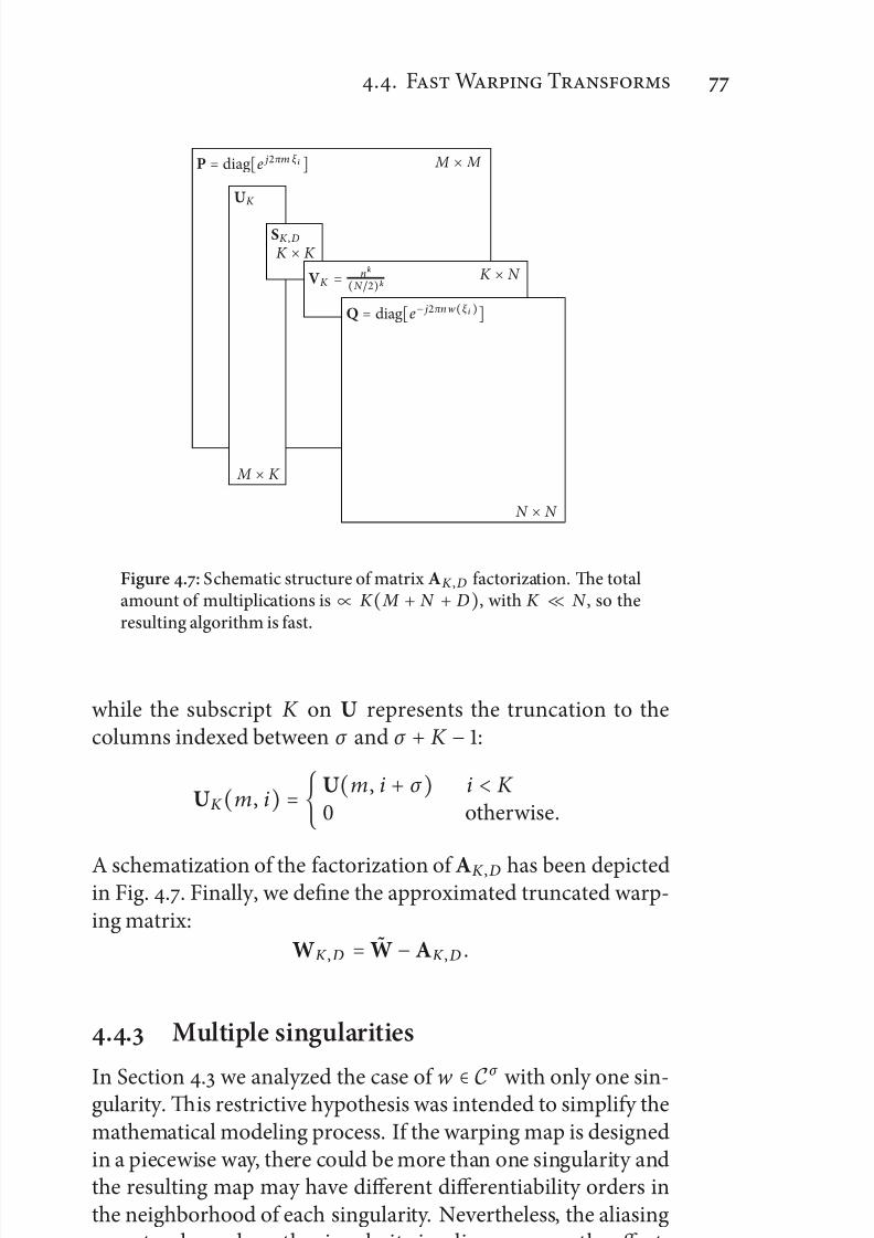
7/21/2019 Design and Computation of Warped Time-Frequency Transforms
http://slidepdf.com/reader/full/design-and-computation-of-warped-time-frequency-transforms 97/150
.. F W T
P = diag[e jπm ξ i ] M × M
UK
M × K
SK ,D
K × K
VK = nk
(N )kK × N
Q = diag[e− jπnw (ξ i )]
N × N
Figure .: Schematic structure of matrix AK ,D factorization. e totalamount of multiplications is ∝ K ( M + N + D), with K ≪ N , so theresulting algorithm is fast.
while the subscript K on U represents the truncation to thecolumns indexed between σ and σ + K − :
UK (m, i) = U(m, i + σ ) i < K otherwise.
A schematization of the factorization of AK ,D has been depictedin Fig. .. Finally, we define the approximated truncated warp-ing matrix:
WK ,D = W −AK ,D .
.. Multiple singularities
In Section . we analyzed the case of w ∈ Cσ
with only one sin-gularity. is restrictive hypothesis was intended to simplify themathematical modeling process. If the warping map is designedin a piecewise way, there could be more than one singularity andthe resulting map may have different differentiability orders inthe neighborhood of each singularity. Nevertheless, the aliasingoperator depends on the singularity in a linear way, so the effectsof multiple singularities superimpose linearly.
7/21/2019 Design and Computation of Warped Time-Frequency Transforms
http://slidepdf.com/reader/full/design-and-computation-of-warped-time-frequency-transforms 98/150
C . F A
We remind that the warping map w( f ) has to be an oddfunction in order to guarantee that a real signal is transformedinto a real signal. If we suppose to have L singularities ξ l , l = , . . . , L, ξ l ∈ (, ) generating the aliasing matrixes A(ξ l ), theneach singularity must have a corresponding dual singularity in − ξ l or equivalently in −ξ l generating A(−ξ l ), which can beshown to be equal to A(ξ l )∗. So, the effect of each singularity in ξ l ∈ (, ) is given by:
A(ξ l )+A(−ξ l ) = R[A(ξ l )].
If present, the singularities in and do not have any dualsingularities and generate the aliasing matrixes A() and A()
respectively. So, by superimposing the effects of all potentialsingularities, it results:
A = A()+A()
+
L
l =
R[A(ξ l )]For A() and A() some simplifications occur. If ξ = ,
both P and Q are equal to the identity matrix since w() = ,and therefore can be neglected. If ξ = , since w() = ,matrixes P and Q just cause a sign inversion on odd indexedinput and output entries. In both cases, for the output to be real,S must have real entries as well. Moreover, the differentiability orders σ and σ must be odd, since Dσ +w must be an oddfunction to have a step on ξ = or ξ = . erefore, fromequation (.), it follows that even diagonals of S are null.
. Performances
In order to evaluate the accuracy of the proposed algorithm wemust introduce a measure of the reconstruction error. As donebefore, the measure is assumed to be the spectral norm of thereconstruction error matrix, i.e. the maximum its eigenvalue.
erefore, we first consider the error in the ideal case, which isgiven by operator W itself:
εW = W†W − IN = E†E.
As the worst case, we consider the error given by operator W,which means no aliasing compensation:
ε W =
W†W − IN
.

7/21/2019 Design and Computation of Warped Time-Frequency Transforms
http://slidepdf.com/reader/full/design-and-computation-of-warped-time-frequency-transforms 99/150
.. P
en, we consider the error in approximating the ideal operatorW†W:
є WK ,D =
W†K ,D WK ,D −W†W
which is intended to check the convergence of the representationintroduced for A. is parameter is lower limited by and upperlimited by є W = W† W −W†W ≃ ε W:
≤ є WK ,D ≤ є W .
Here we will show that it is not required to make є WK ,D reach
its lower limit. In fact, in order to evaluate performances, weintroduce the error εWK ,D
:
εWK ,D = W†
K ,D WK ,D − IN .
such thatεW ≤ εWK ,D
≤ ε W .
For both є WK ,D and εWK ,D
, the upper limit є W ≃ ε W is obtained
for K = and/or D = (no aliasing compensation), while thelower limit is theoretically reached for K , D → ∞. Nevertheless,since S entries decrease exponentially, we expect that є WK ,D
andεWK ,D
decrease exponentially as well. In particular, εWK ,D reaches
the target value εW for values of K and D much smaller than N :
εWK ,D = W†
K ,D WK ,D −W†W +W†W − IN ≤
W†K ,D WK ,D −W†W
+
W†W − IN
≤ є WK ,D + εW (.)
≃ max[ є WK ,D, εW ]. (.)
us, the truncation of S turns the complexity from O(N )to O(N ), like in a truncated Singular Value Decomposition. Infact, the matrix-vector multiplication involving VK , SK ,D andUK requires K ⋅ N , K ⋅ D and K ⋅ M multiplications respectively,
while the scaling by P and Q is computed by M +
N multiplica-tions, hence about K ⋅ (N + M + D) multiplications are needed.In order to evaluate the accuracy of the proposed algorithm,
we numerically computed the spectral norms є WK ,D and εWK ,D
for the frequency warping map (.) which belong to C , withmax w = for N = and M = N .
In Fig. . we plotted є WK ,D respect to K and for increasing
values of of D. As expected, it decreases exponentially as K
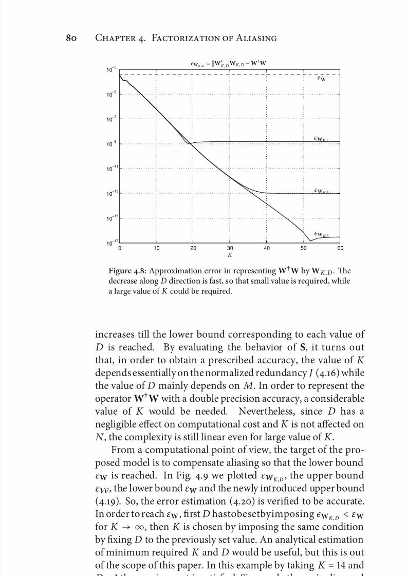
7/21/2019 Design and Computation of Warped Time-Frequency Transforms
http://slidepdf.com/reader/full/design-and-computation-of-warped-time-frequency-transforms 100/150
C . F A
0 10 20 30 40 50 6010
−17
10−15
10−13
10−11
10−9
10−7
10−5
10−3
є WK ,D = W†
K ,D WK ,D −W† W
K
є W
є WK ,
є WK ,
є WK ,
Figure .: Approximation error in representing W†W by WK ,D . edecrease along D direction is fast, so that small value is required, whilea large value of K could be required.
increases till the lower bound corresponding to each value of D is reached. By evaluating the behavior of S, it turns outthat, in order to obtain a prescribed accuracy, the value of K depends essentially on the normalized redundancy J (.) whilethe value of D mainly depends on M . In order to represent the
operator W
†
W with a double precision accuracy, a considerable value of K would be needed. Nevertheless, since D has anegligible effect on computational cost and K is not affected onN , the complexity is still linear even for large value of K .
From a computational point of view, the target of the pro-posed model is to compensate aliasing so that the lower boundεW is reached. In Fig. . we plotted εWK ,D
, the upper boundεW , the lower bound εW and the newly introduced upper bound
(.). So, the error estimation (.) is verified to be accurate.In order to reach εW , first D hastobesetbyimposing є WK ,D < εW
for K → ∞, then K is chosen by imposing the same conditionby fixing D to the previously set value. An analytical estimationof minimum required K and D would be useful, but this is outof the scope of this paper. In this example by taking K = andD = the requirement is satisfied. Since only the main diagonalis needed, SK , is easily obtained by βk , (.) and γk , (.).
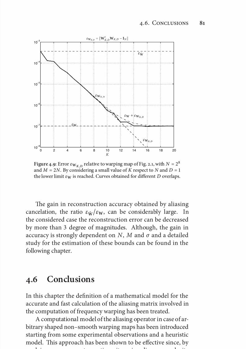
7/21/2019 Design and Computation of Warped Time-Frequency Transforms
http://slidepdf.com/reader/full/design-and-computation-of-warped-time-frequency-transforms 101/150
.. C
0 2 4 6 8 10 12 14 16 18 2010
−8
10−7
10−6
10−5
10−4
10−3
εWK ,D = W†
K , D WK , D − IN
K
εW
ε W
εWK ,D
є WK ,D
εW + є WK ,D
Figure .: Error εWK ,D relative to warping map of Fig. ., with N =
and M = N . By considering a small value of K respect to N and D = the lower limit εW is reached. Curves obtained for different D overlaps.
e gain in reconstruction accuracy obtained by aliasingcancelation, the ratio ε WεW, can be considerably large. Inthe considered case the reconstruction error can be decreasedby more than degree of magnitudes. Although, the gain inaccuracy is strongly dependent on N , M and σ and a detailed
study for the estimation of these bounds can be found in thefollowing chapter.
. Conclusions
In this chapter the definition of a mathematical model for the
accurate and fast calculation of the aliasing matrix involved inthe computation of frequency warping has been treated.A computational model of the aliasing operator in case of ar-
bitrary shaped non–smooth warping maps has been introducedstarting from some experimental observations and a heuristicmodel. is approach has been shown to be effective since, by applying some proper truncations, it carries a linear complexity without compromising reconstruction accuracy.
7/21/2019 Design and Computation of Warped Time-Frequency Transforms
http://slidepdf.com/reader/full/design-and-computation-of-warped-time-frequency-transforms 102/150
C . F A
Appendix .A Mathematical Proofs
.A. Expressions of functions ψ i
In order to derive the expression of ψ i , we start by derivingequation (.):
Dψ i( f ) = H ( f ) f (i−)
(i − )! −
i+
k=
ρ i+, k k f k−
= H
( f
) f (i−)
(i −
)! −
i
k=
ρ i+, k+
(k +
) f k
which still matches the definition of ψ i− by considering:
ρ i ,k = (k + ) ρi+, k+ k = , . . . , i
By iteratively applying k times this equation to (.) we get:
ψ i
( f
) = H
( f
)
i! f i −
i+
k=
k! f k ρ i+−k (.)
where the second subscript has been omitted being equal to .Now we impose the functions ψ i to be periodic, i.e. ψ i() =ψ i():
i!−
i+
k=
ρ i+−k
k!=
so that for ρ i we have:
ρi =
i! −
i
k=
ρ i−k(k + )!
which, starting from ρ = , generates the following sequence:
, , , , −, , , , −, . . .
to be used in (.) to generate ψ i functions.
.A. Factorization of D i f ϕn
e factorization (.) will be demonstrated to be true by in-duction. To simplify the notation, we set µ = − jπ nw. First we verify it is true for i = :
ϕn = α, enµ ⇒ α, =
(Dw
) .

7/21/2019 Design and Computation of Warped Time-Frequency Transforms
http://slidepdf.com/reader/full/design-and-computation-of-warped-time-frequency-transforms 103/150
.A. M P
en, we suppose it is true for i − :
D
i−
ϕn = e
µi−
k= αi−, i−−k(Dµ)k
and try to verify it implies that the factorization is true for i . By deriving the factorization of D i−ϕn we get:
Dµe µi−
k=
αi−, i−−k(Dµ)k+ e µ D
i−
k=
α i−, i−−k(Dµ)k
and we try to express it as a polynomial in Dµ. For the first termwe have:
enµi
k=
α i−, i−k(nDµ)k
while for the second term:
e µi−
k=[Dα i−, i−−k
(Dµ
)k+ αi−, i−−k k
(Dµ
)k−D µ
] =e µ
i−
k=
Dα i−, i−−k + αi−, i−−k kDw(Dw)− (Dµ)k
so that D i ϕn has been expressed as a polynomial in Dµ withpower from to i, as it was required. en we impose theexpression of coefficients α i , i−k . e coefficient of
(Dµ
)i is:
αi , = α i−, ⇒ αi , = α, = (Dw)
while the coefficient of (Dµ)i :
α i , i = D αi−, i− . (.)
e rest of the coefficients are given in differential form:
αi ,k − α i−, k =Dαi−, k− + α i−, k−(i − k)Dw(Dw)− . (.)
.A. Expressions of coefficients α i,k
We will first demonstrate by induction that α can be factorize asin (.). For k = the factorization is true since α i , =
(Dw
).
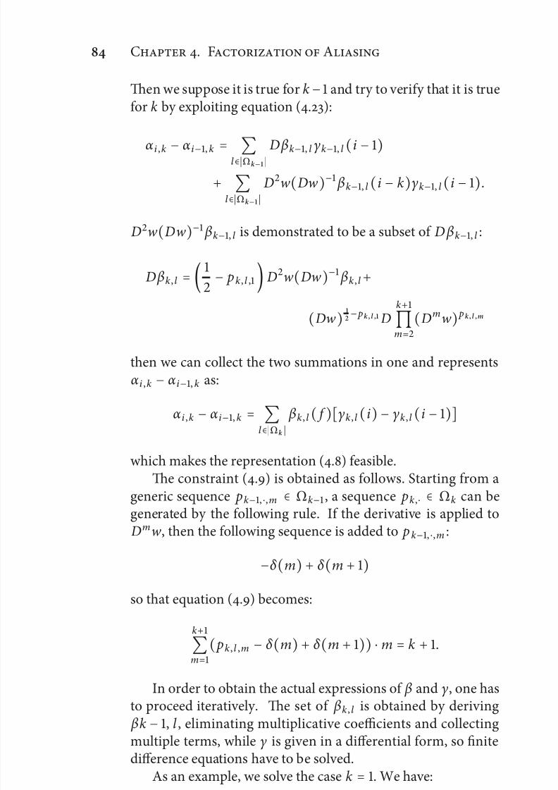
7/21/2019 Design and Computation of Warped Time-Frequency Transforms
http://slidepdf.com/reader/full/design-and-computation-of-warped-time-frequency-transforms 104/150
C . F A
en we suppose it is true for k− and try to verify that it is truefor k by exploiting equation (.):
α i ,k − αi−, k = l ∈Ωk−
D βk−, l γk−, l (i − )+
l ∈Ωk−
Dw(Dw)− βk−, l (i − k)γk−, l (i − ).
Dw(Dw)− βk−, l is demonstrated to be a subset of D βk−, l :
D βk , l =
− pk , l ,Dw(Dw)− βk , l +
(Dw) − pk , l , D
k+
m=
(Dmw) pk , l ,m
then we can collect the two summations in one and representsαi ,k − αi−, k as:
α i ,k − αi−, k = l ∈Ωk βk , l ( f )[γk , l (i)− γk , l (i − )]
which makes the representation (.) feasible.e constraint (.) is obtained as follows. Starting from a
generic sequence pk−, ⋅,m ∈ Ωk− , a sequence pk ,⋅ ∈ Ωk can begenerated by the following rule. If the derivative is applied toDmw, then the following sequence is added to p k−, ⋅,m :
−δ (m)+ δ (m + )so that equation (.) becomes:
k+
m=
( pk , l ,m − δ (m)+ δ (m + )) ⋅ m = k + .
In order to obtain the actual expressions of β and γ, one hasto proceed iteratively. e set of βk , l is obtained by deriving βk − , l , eliminating multiplicative coefficients and collectingmultiple terms, while γ is given in a differential form, so finitedifference equations have to be solved.
As an example, we solve the case k = . We have:
β, = Dw
(Dw
)−
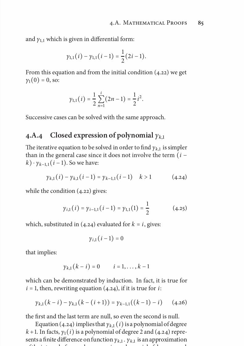
7/21/2019 Design and Computation of Warped Time-Frequency Transforms
http://slidepdf.com/reader/full/design-and-computation-of-warped-time-frequency-transforms 105/150
.A. M P
and γ, which is given in differential form:
γ,
(i
)− γ,
(i −
) =
(i −
).
From this equation and from the initial condition (.) we getγ() = , so:
γ, (i) =
i
n=
(n − ) =
i .
Successive cases can be solved with the same approach.
.A. Closed expression of polynomial γk,
e iterative equation to be solved in order to find γk , is simplerthan in the general case since it does not involve the term (i −k) ⋅ γk−, (i − ). So we have:
γk ,
(i
)− γk ,
(i −
) = γk−,
(i −
) k > (.)
while the condition (.) gives:
γ i ,(i) = γ i−, (i − ) = γ, () =
(.)
which, substituted in (.) evaluated for k = i , gives:
γi ,
(i −
) =
that implies:
γk ,(k − i) = i = , . . . , k −
which can be demonstrated by induction. In fact, it is true fori = , then, rewriting equation (.), if it is true for i :
γk ,(k − i)− γk ,(k − (i + )) = γk−, ((k − ) − i) (.)
the first and the last term are null, so even the second is null.Equation (.) implies that γk , (i) is a polynomial of degree
k+ . In facts, γ(i) is a polynomial of degree and (.) repre-sents a finite difference on function γk , . γk , is an approximationof the integral of γk−, , hence γk , is a polynomial of degree equalto degree of γk−, plus . In order to determine a polynomial of
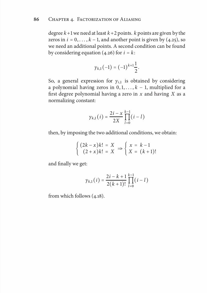
7/21/2019 Design and Computation of Warped Time-Frequency Transforms
http://slidepdf.com/reader/full/design-and-computation-of-warped-time-frequency-transforms 106/150
C . F A
degree k+ we need at least k+ points. k points are given by thezeros in i = , . . . , k − , and another point is given by (.), sowe need an additional points. A second condition can be found
by considering equation (.) for i = k :
γk ,(−) = (−)k+
.
So, a general expression for γi , is obtained by consideringa polynomial having zeros in , , . . . , k − , multiplied for afirst degree polynomial having a zero in x and having X as a
normalizing constant:
γk ,(i) = i − x
X
k−
l =
(i − l )then, by imposing the two additional conditions, we obtain:
(k − x
)k! = X
(+
x )k! = X
⇒
x = k −
X = (k+
)!
and finally we get:
γk ,(i) = i − k +
(k + )!
k−
l =
(i − l )from which follows (.).

7/21/2019 Design and Computation of Warped Time-Frequency Transforms
http://slidepdf.com/reader/full/design-and-computation-of-warped-time-frequency-transforms 107/150

7/21/2019 Design and Computation of Warped Time-Frequency Transforms
http://slidepdf.com/reader/full/design-and-computation-of-warped-time-frequency-transforms 108/150

7/21/2019 Design and Computation of Warped Time-Frequency Transforms
http://slidepdf.com/reader/full/design-and-computation-of-warped-time-frequency-transforms 109/150
C
Frame Bounds
Estimation
W has been introduced in this work in the frame-
work of unitary operators. is point of view has ledthe derivation of a time-discrete frequency warping operator asan infinite-dimensional matrix, which, despite of being unitary,could not be used in a practical sense. For these reason, weintroduced some finite-dimensional variants which, in order tomaintain the capability of recovering the original signal fromthe transformed one by the application of their adjoints, mustproduce a redundant output, i.e. a transformed output signallonger than the input one.
Unitary property is a characteristic of square operators, sinceneither the direct transformation nor the adjoint one can be sin-gular. So, the rectangular operators which have been describedin this work can not be categorized as unitary. Instead, they must be considered in the framework of frames [, ]. In thistheory, the property of being unitary is replaced by the property of being a tight frame. e frame refers to the fact that, if weconsider the adjoint operator composed with the direct one, itsmaximum and minimum eigenvalues are positive, so that allthe eigenvalues are enclosed in the frame determined by theminimum and the maximum one, called frame bounds. etight property takes place when the frame bounds collapse onthe same value, so that all the eigenvalues have the same value.erefore, frame bounds are related to reconstruction accuracy.
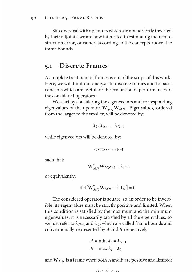
7/21/2019 Design and Computation of Warped Time-Frequency Transforms
http://slidepdf.com/reader/full/design-and-computation-of-warped-time-frequency-transforms 110/150
C . F B
Since we deal with operators which are not perfectly invertedby their adjoints, we are now interested in estimating the recon-struction error, or rather, according to the concepts above, the
frame bounds.
. Discrete Frames
A complete treatment of frames is out of the scope of this work.Here, we will limit our analysis to discrete frames and to basicconcepts which are useful for the evaluation of performances of
the considered operators.We start by considering the eigenvectors and corresponding
eigenvalues of the operator W† M N W MN . Eigenvalues, ordered
from the larger to the smaller, will be denoted by:
λ , λ , . . . , λN −
while eigenvectors will be denoted by:
v , v , . . . , v N −
such that:
W† MN W M N v i = λi v i
or equivalently:
det
[W†
M N W
MN − λ
iI
N ] = .
e considered operator is square, so, in order to be invert-ible, its eigenvalues must be strictly positive and limited. Whenthis condition is satisfied by the maximum and the minimumeigenvalues, it is necessarily satisfied by all the eigenvalues, sowe just refer to λ N − and λ, which are called frame bounds andconventionally represented by A and B respectively:
A= min λi = λN −
B = max λi = λ
and W M N is a frame when both A and B are positive and limited:
< A < ∞ < B < ∞.
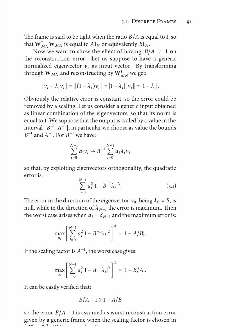
7/21/2019 Design and Computation of Warped Time-Frequency Transforms
http://slidepdf.com/reader/full/design-and-computation-of-warped-time-frequency-transforms 111/150
.. D F
e frame is said to be tight when the ratio B A is equal to , sothat W†
M N W M N is equal to AIN or equivalently BIN .Now we want to show the effect of having B
A ≠ on
the reconstruction error. Let us suppose to have a genericnormalized eigenvector v i as input vector. By transformingthrough W M N and reconstructing by W†
M N we get:
v i − λi v i = ( − λi)v i = − λ i v i = − λi .Obviously the relative error is constant, so the error could beremoved by a scaling. Let us consider a generic input obtained
as linear combination of the eigenvectors, so that its norm isequal to . We suppose that the output is scaled by a value in theinterval [B− , A−], in particular we choose as value the bounds
B− and A− . For B− we have:
N −
i=
a iv i ↦ B−N −
i=
a i λi v i
so that, by exploiting eigenvectors orthogonality, the quadraticerror is:N −
i=
ai − B− λi . (.)
e error in the direction of the eigenvector v , being λ = B, isnull, while in the direction of λ N − the error is maximum. enthe worst case arises when a i = δ N − and the maximum error is:
maxa i
N −i=
ai − B− λi
⁄
= − AB.If the scaling factor is A− , the worst case gives:
maxa i
N −
i=
ai − A− λi ⁄
= − B A.It can be easily verified that:
B A− ≥ − AB
so the error B A − is assumed as worst reconstruction errorgiven by a generic frame when the scaling factor is chosen in[B− , A−]. is means that the reconstruction error is upperlimited when an estimation of frame bounds can be performed.
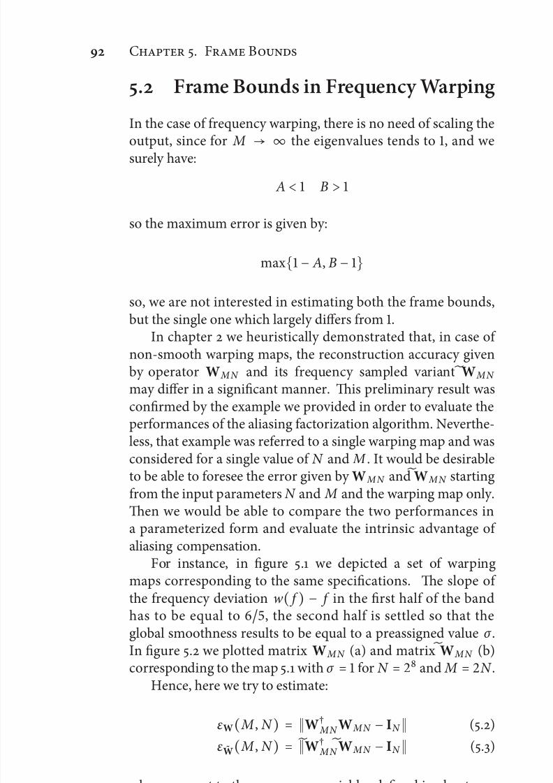
7/21/2019 Design and Computation of Warped Time-Frequency Transforms
http://slidepdf.com/reader/full/design-and-computation-of-warped-time-frequency-transforms 112/150
C . F B
. Frame Bounds in Frequency Warping
In the case of frequency warping, there is no need of scaling the
output, since for M → ∞ the eigenvalues tends to , and wesurely have:
A < B >
so the maximum error is given by:
max
− A, B −
so, we are not interested in estimating both the frame bounds,but the single one which largely differs from .
In chapter we heuristically demonstrated that, in case of non-smooth warping maps, the reconstruction accuracy givenby operator W M N and its frequency sampled variant W M N
may differ in a significant manner. is preliminary result was
confirmed by the example we provided in order to evaluate theperformances of the aliasing factorization algorithm. Neverthe-less, that example was referred to a single warping map and wasconsidered for a single value of N and M . It would be desirableto be able to foresee the error given by W M N and W M N startingfrom the input parameters N and M and the warping map only.en we would be able to compare the two performances ina parameterized form and evaluate the intrinsic advantage of
aliasing compensation.For instance, in figure . we depicted a set of warping
maps corresponding to the same specifications. e slope of the frequency deviation w( f ) − f in the first half of the bandhas to be equal to , the second half is settled so that theglobal smoothness results to be equal to a preassigned value σ .In figure . we plotted matrix W M N (a) and matrix W M N (b)corresponding to the map . with σ = for N = and M = N .
Hence, here we try to estimate:
εW( M , N ) = W† MN W M N − IN (.)
ε W( M , N ) = W† MN
W M N − IN (.)
where, respect to the same error variables defined in chapter ,we pointed out a dependency on M and N .

7/21/2019 Design and Computation of Warped Time-Frequency Transforms
http://slidepdf.com/reader/full/design-and-computation-of-warped-time-frequency-transforms 113/150
.. E E
0 0.5 1−0.1
0
0.1
0 0.5 1−0.1
0
0.1
0 0.5 1−0.1
0
0.1
0 0.5 1−0.1
0
0.1
wσ ( f ) − f , σ = wσ ( f ) − f , σ =
wσ ( f ) − f , σ = wσ ( f ) − f , σ =
f f
f f
Figure .: Frequency deviation, i.e. w ( f )− f , of the warping maps usedin the for evaluating the performances of the frame bounds estimation.e warping maps are obtained in a piecewise way: in the interval[, ] they are equal to a line of slope , in the interval [, ]they are polynomials of odd powers giving σ continuous derivatives on
the singularity point .
. Error Estimation
e estimation procedure take advantage of the tails matrix andaliasing model which was developed in chapter .
As far as (.) is concerned, we recall that εW is equal to
E† M N E MN and that E M N can be factorized by (.). Withproper hypothesis when multiple singularities are considered,we reduce to the following:
εW = V†S†Y†YSVthen S is substituted by the σ -th lower diagonal, Y†Y, which isanalytically computable and proportional to M , is substituted
by the σ -th entry of the main diagonal and the effect of V isrepresented by a factor N . Finally we get:
εW ≃ ρ( M N )π σ +(σ + ) ⋅ N
M σ + ⋅ ∆ (.)
where ∆ is the differential value between ξ + and ξ − of βσ , (.):
∆ = βσ ,
(ξ +
)− βσ ,
(ξ −
)
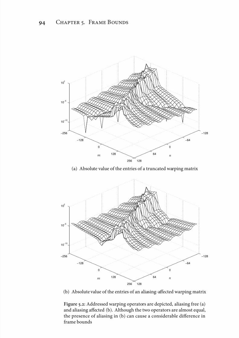
7/21/2019 Design and Computation of Warped Time-Frequency Transforms
http://slidepdf.com/reader/full/design-and-computation-of-warped-time-frequency-transforms 114/150
C . F B
−128
−64
0
64
128
−256
−128
0
128
256
10−10
10−5
100
nm
(a) Absolute value of the entries of a truncated warping matrix
−128
−64
0
64
128
−256
−128
0
128
256
10−10
10−5
100
nm
(b) Absolute value of the entries of an aliasing-affected warping matrix
Figure .: Addressed warping operators are depicted, aliasing free (a)and aliasing affected (b). Although the two operators are almost equal,the presence of aliasing in (b) can cause a considerable difference inframe bounds

7/21/2019 Design and Computation of Warped Time-Frequency Transforms
http://slidepdf.com/reader/full/design-and-computation-of-warped-time-frequency-transforms 115/150
.. E E
0
5
10
15
20
25
0
5
10
15
20
250
0.5
1
1.5
2
2.5
x 10−6
Figure .: Absolutevalue of matrix S entries for σ = , N = and M =N . Most of the energy is concentrated along the σ -th lower diagonal.
while ρ is the maximum of the polynomial γσ , (.) corre-sponding to βσ , multiplied for a negative exponential having J (.) as base:
ρ = max x
[ J (ξ )− x +σ γσ ,(x )](.)
which corresponds to the square maximum of the σ -th lower
diagonal of S (see fig. .). e expression (.) has to beslightly modified in the case σ = . A quasi-exact analyticalsolution will be provided for ρ, by assuming that the variable x is continuous, although, being a vector index, would be discrete.So we compute the maximum by calculating the value nullifyingthe first derivative:
Dγσ ,
(x
) = γσ ,
(x
)log J
e polynomial γσ , has degree equal to σ + and gets an even orodd symmetry if shied back by (σ −). It follows that γσ ,(x +(σ − )) has either even or odd powers and its derivative canbe approximated by:
Dγk ,
x +
σ −
≃ D
x +
σ −
σ +
=
(σ +
) x +
σ −
σ

7/21/2019 Design and Computation of Warped Time-Frequency Transforms
http://slidepdf.com/reader/full/design-and-computation-of-warped-time-frequency-transforms 116/150
C . F B
and finally we get the following approximated solution:
x ≃ σ +
log J −
σ −
.
We point out that, representing a positive index, one has toprevent this solution to become smaller than .
In order to estimate ε W we take advantage of equation (.):
ε W ≃ W† M N A M N = A†
MN W M N W† M N A M N .
For σ > the product W M N W† MN can be safely substituted by itsmain diagonal, whose shape can be analytically derived startingfrom the warping map. en the model (.) is substituted andit turns out:
ε W ≃ V†S†U†CUSV (.)
where diag(C) = diag(W M N W† M N ). en only an estimation
for diag
(U†CU
) is needed to trace the estimation of ε W back to
the form (.). Matrix C has only N max Dw significant values,so that it actually selects the central values of U columns, that isU(m, k) with m ∈ Z⌈N max Dw ⌉ . e σ -th entry of diag(U†CU)results to be the energy of U(m, σ )with m ∈ Z⌈N max Dw ⌉ , whichbehaves like a constant in case σ is odd and like m in case σ iseven. So energies are proportional to M mod(σ +):
ε W ≃ ρ( M N )π σ + ⋅ κN M (σ ++mod(σ +)) ⋅ ∆
. (.)
Incase σ is odd κ is exactly proportional to N according to valuesof D k ζ (). In case σ is even κ is roughly proportional to N buthas to be numerically computed.
e estimations (.) and (.) have been obtained by im-posing the convergence to the exact values for M tending to
∞
. So, apart from a possible lack in accuracy for M closeto N max Dw, these estimations describe the analytical depen-dency of the frame bounds on the design variables N , M andσ . Moreover, they allow to evaluate the advantage obtainedby using the aliasing free frequency warping operator ratherthan the frequency sampled one. Finally, the solution of (.)allows to estimate the required K to make the computation of the aliasing matrix A M N converge.
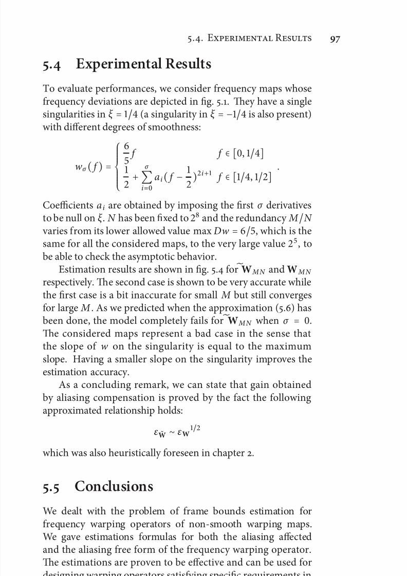
7/21/2019 Design and Computation of Warped Time-Frequency Transforms
http://slidepdf.com/reader/full/design-and-computation-of-warped-time-frequency-transforms 117/150
.. E R
. Experimental Results
To evaluate performances, we consider frequency maps whose
frequency deviations are depicted in fig. .. ey have a singlesingularities in ξ = (a singularity in ξ = − is also present)with different degrees of smoothness:
wσ ( f ) =⎧⎪⎪⎪⎪⎪⎨⎪⎪⎪⎪⎪⎩
f f ∈ [, ]
+
σ
i=
a i( f −
)i+ f ∈ [, ] .
Coefficients a i are obtained by imposing the first σ derivativesto be null on ξ . N has been fixed to and the redundancy M N varies from its lower allowed value max Dw = , which is thesame for all the considered maps, to the very large value , tobe able to check the asymptotic behavior.
Estimation results are shown in fig. . for W M N and W M N
respectively. e second case is shown to be very accurate whilethe first case is a bit inaccurate for small M but still convergesfor large M . As we predicted when the approximation (.) hasbeen done, the model completely fails for W M N when σ = .
e considered maps represent a bad case in the sense thatthe slope of w on the singularity is equal to the maximumslope. Having a smaller slope on the singularity improves theestimation accuracy.
As a concluding remark, we can state that gain obtainedby aliasing compensation is proved by the fact the followingapproximated relationship holds:
ε W ∼ εW
which was also heuristically foreseen in chapter .
. Conclusions
We dealt with the problem of frame bounds estimation forfrequency warping operators of non-smooth warping maps.We gave estimations formulas for both the aliasing affectedand the aliasing free form of the frequency warping operator.e estimations are proven to be effective and can be used fordesigning warping operators satisfying specific requirements inreconstruction accuracy.
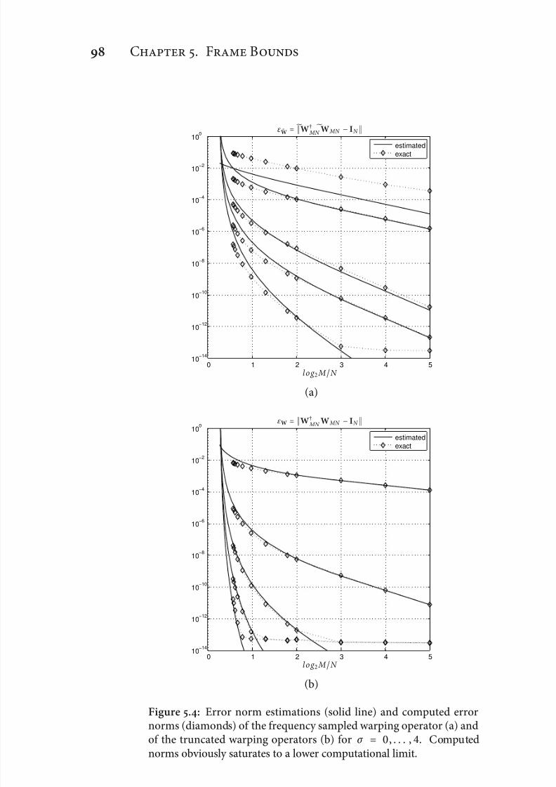
7/21/2019 Design and Computation of Warped Time-Frequency Transforms
http://slidepdf.com/reader/full/design-and-computation-of-warped-time-frequency-transforms 118/150
C . F B
0 1 2 3 4 510
−14
10−12
10−10
10−8
10−6
10−4
10−2
100
estimated
exact
ε W =
W† MN
W MN − IN
log M N
(a)
0 1 2 3 4 510
−14
10−12
10−10
10−8
10−6
10−4
10−2
100
estimated
exact
εW = W† MN W MN − IN
log M N
(b)
Figure .: Error norm estimations (solid line) and computed errornorms (diamonds) of the frequency sampled warping operator (a) andof the truncated warping operators (b) for σ = , . . . , . Computednorms obviously saturates to a lower computational limit.

7/21/2019 Design and Computation of Warped Time-Frequency Transforms
http://slidepdf.com/reader/full/design-and-computation-of-warped-time-frequency-transforms 119/150

7/21/2019 Design and Computation of Warped Time-Frequency Transforms
http://slidepdf.com/reader/full/design-and-computation-of-warped-time-frequency-transforms 120/150

7/21/2019 Design and Computation of Warped Time-Frequency Transforms
http://slidepdf.com/reader/full/design-and-computation-of-warped-time-frequency-transforms 121/150
P
IIIApplications on
Ultrasound Signals

7/21/2019 Design and Computation of Warped Time-Frequency Transforms
http://slidepdf.com/reader/full/design-and-computation-of-warped-time-frequency-transforms 122/150
7/21/2019 Design and Computation of Warped Time-Frequency Transforms
http://slidepdf.com/reader/full/design-and-computation-of-warped-time-frequency-transforms 123/150
C
Ultrasonic Guided
Waves Characterization
G Waves (GWs) have characteristic dispersive time-
frequency representations (TFRs). Unfortunately, any TFR is subjected to the time-frequency uncertainty principle. is,in general, limits the capability of TFRs to characterize multiple,closely spaced guided modes from a time transient measure-ment, over a wide frequency range. To overcome this limitation,we present here a new warped frequency transform (WFT) thatin force of a more flexible tiling of the time frequency domainpresents enhanced modes extraction capabilities. Such tilingis chosen to match the dispersive spectro-temporal structureof the waveguide by selecting an appropriate map of the timefrequency plane. e proposed transformation is fast, invertible,and covariant to group delay shis. In particular, in this chapterwe describe design and calculation strategies for maps tailoredto Lamb waves propagating in an aluminium plate. Time-transient guided wave propagation events obtained both artifi-cially and experimentally are considered. e results show thatthe proposed WFT limits interference patterns which appearswith others TFRs and produces a sparse representation of theLamb waves pattern that can be suitable for identification andcharacterization purposes.
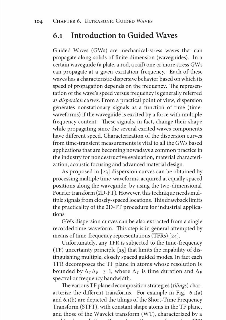
7/21/2019 Design and Computation of Warped Time-Frequency Transforms
http://slidepdf.com/reader/full/design-and-computation-of-warped-time-frequency-transforms 124/150
C . U G W
. Introduction to Guided Waves
Guided Waves (GWs) are mechanical-stress waves that can
propagate along solids of finite dimension (waveguides). In acertain waveguide (a plate, a rod, a rail) one or more stress GWscan propagate at a given excitation frequency. Each of thesewaves has a characteristic dispersive behavior based on which itsspeed of propagation depends on the frequency. e represen-tation of the wave’s speed versus frequency is generally referredas dispersion curves. From a practical point of view, dispersiongenerates nonstationary signals as a function of time (time-waveforms) if the waveguide is excited by a force with multiplefrequency content. ese signals, in fact, change their shapewhile propagating since the several excited waves componentshave different speed. Characterization of the dispersion curvesfrom time-transient measurements is vital to all the GWs basedapplications that are becoming nowadays a common practice inthe industry for nondestructive evaluation, material characteri-zation, acoustic focusing and advanced material design.
As proposed in [] dispersion curves can be obtained by processing multiple time-waveforms, acquired at equally spacedpositions along the waveguide, by using the two-dimensionalFourier transform (D-FT). However, this technique needs mul-tiple signals from closely-spaced locations. is drawback limitsthe practicality of the D-FT procedure for industrial applica-tions.
GWs dispersion curves can be also extracted from a singlerecorded time-waveform. is step is in general attempted by means of time-frequency representations (TFRs) [].
Unfortunately, any TFR is subjected to the time-frequency (TF) uncertainty principle [] that limits the capability of dis-tinguishing multiple, closely spaced guided modes. In fact eachTFR decomposes the TF plane in atoms whose resolution isbounded by ∆T ∆F ≥ , where ∆T is time duration and ∆F
spectral or frequency bandwidth.e various TF plane decomposition strategies (tilings) char-acterize the different transforms. For example in Fig. .(a)and .(b) are depicted the tilings of the Short-Time Frequency Transform (STFT), with constant shape atoms in the TF plane,and those of the Wavelet transform (WT), characterized by amultiscale resolution. Processing a time waveform via a TFR produces a complex coefficient for each atom of the TF plane.
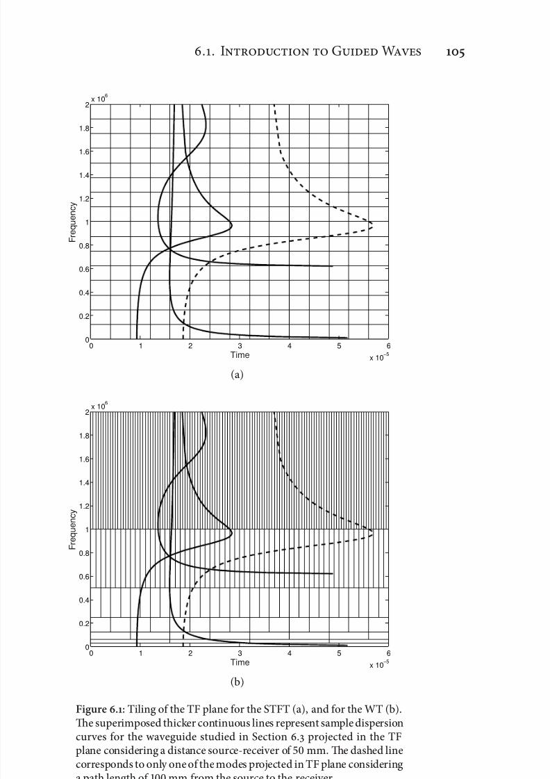
7/21/2019 Design and Computation of Warped Time-Frequency Transforms
http://slidepdf.com/reader/full/design-and-computation-of-warped-time-frequency-transforms 125/150
.. I G W
0 1 2 3 4 5 6
x 10−5
0
0.2
0.4
0.6
0.8
1
1.2
1.4
1.6
1.8
2x 10
6
Time
F r e q u e n c y
(a)
0 1 2 3 4 5 6
x 10−5
0
0.2
0.4
0.6
0.8
1
1.2
1.4
1.6
1.8
2 x 10
6
Time
F r e q u e n c y
(b)
Figure .: Tiling of the TF plane for the STFT (a), and for the WT (b).e superimposed thicker continuous lines represent sample dispersioncurves for the waveguide studied in Section . projected in the TFplane considering a distance source-receiver of mm. e dashed linecorresponds to only one of the modes projected in TF plane consideringa path length of mm from the source to the receiver.
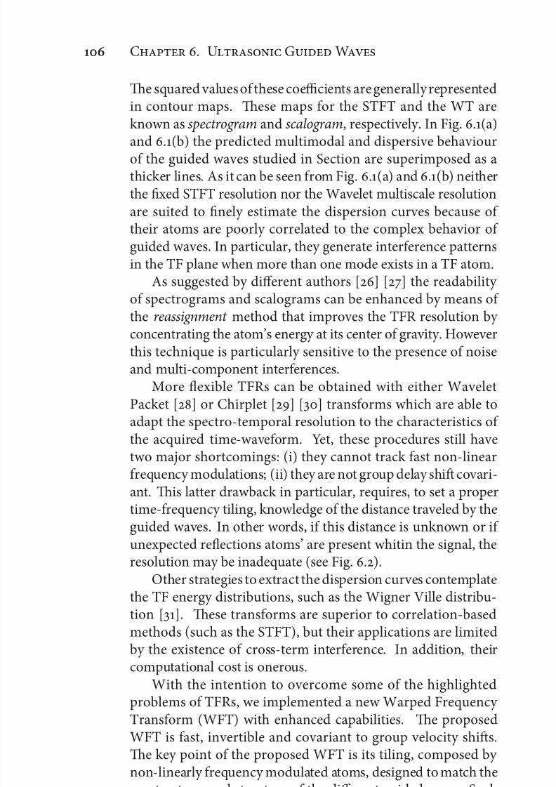
7/21/2019 Design and Computation of Warped Time-Frequency Transforms
http://slidepdf.com/reader/full/design-and-computation-of-warped-time-frequency-transforms 126/150
C . U G W
e squared values of these coefficients are generally representedin contour maps. ese maps for the STFT and the WT areknown as spectrogram and scalogram, respectively. In Fig. .(a)
and .(b) the predicted multimodal and dispersive behaviourof the guided waves studied in Section are superimposed as athicker lines. As it can be seen from Fig. .(a) and .(b) neitherthe fixed STFT resolution nor the Wavelet multiscale resolutionare suited to finely estimate the dispersion curves because of their atoms are poorly correlated to the complex behavior of guided waves. In particular, they generate interference patternsin the TF plane when more than one mode exists in a TF atom.
As suggested by different authors [] [] the readability of spectrograms and scalograms can be enhanced by means of the reassignment method that improves the TFR resolution by concentrating the atom’s energy at its center of gravity. Howeverthis technique is particularly sensitive to the presence of noiseand multi-component interferences.
More flexible TFRs can be obtained with either WaveletPacket [] or Chirplet [] [] transforms which are able toadapt the spectro-temporal resolution to the characteristics of the acquired time-waveform. Yet, these procedures still havetwo major shortcomings: (i) they cannot track fast non-linearfrequency modulations; (ii) they are not group delay shi covari-ant. is latter drawback in particular, requires, to set a propertime-frequency tiling, knowledge of the distance traveled by theguided waves. In other words, if this distance is unknown or if
unexpected reflections atoms’ are present whitin the signal, theresolution may be inadequate (see Fig. .).Other strategies to extract the dispersion curves contemplate
the TF energy distributions, such as the Wigner Ville distribu-tion []. ese transforms are superior to correlation-basedmethods (such as the STFT), but their applications are limitedby the existence of cross-term interference. In addition, theircomputational cost is onerous.
With the intention to overcome some of the highlightedproblems of TFRs, we implemented a new Warped Frequency Transform (WFT) with enhanced capabilities. e proposedWFT is fast, invertible and covariant to group velocity shis.e key point of the proposed WFT is its tiling, composed by non-linearly frequency modulated atoms, designed to match thespectro-temporal structure of the different guided waves. Suchtiling is obtained by selecting an appropriate warping map to
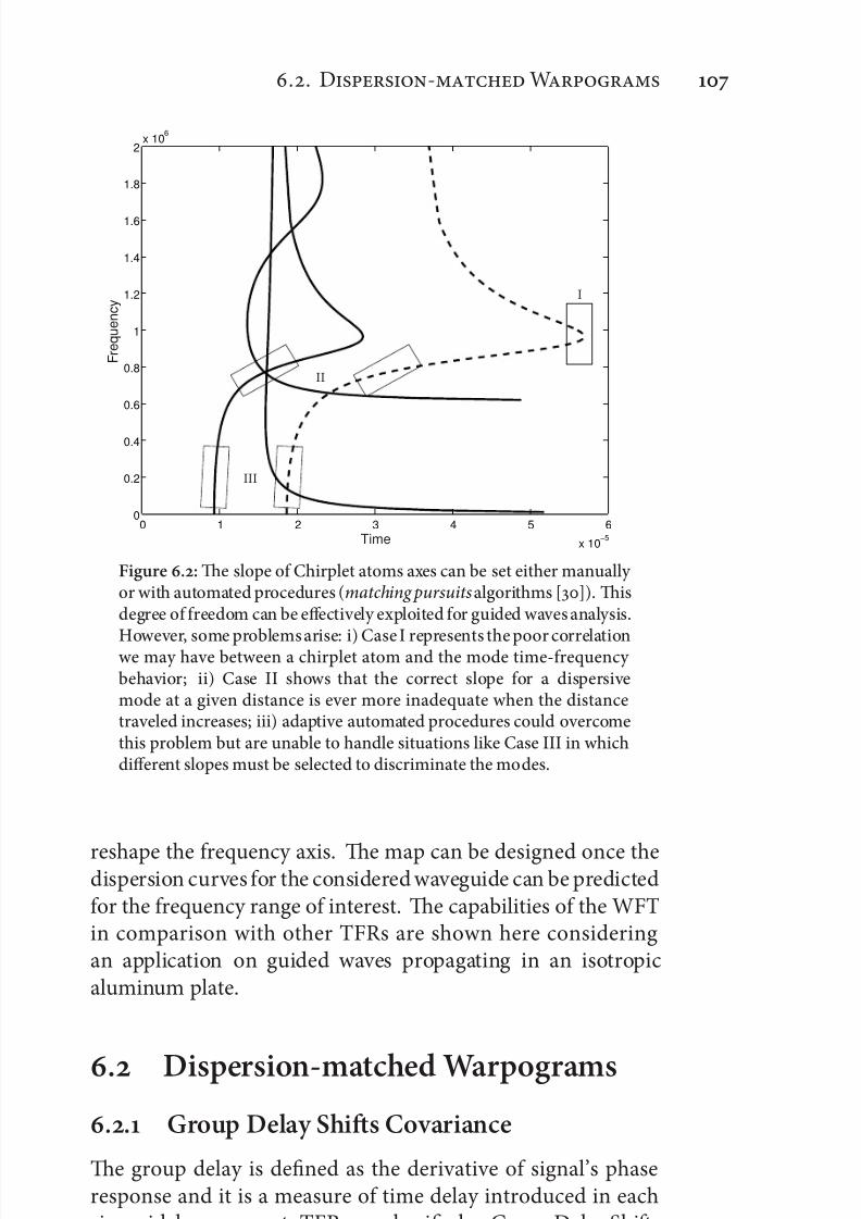
7/21/2019 Design and Computation of Warped Time-Frequency Transforms
http://slidepdf.com/reader/full/design-and-computation-of-warped-time-frequency-transforms 127/150
.. D- W
0 1 2 3 4 5 6
x 10−5
0
0.2
0.4
0.6
0.8
1
1.2
1.4
1.6
1.8
2x 10
6
Time
F r e q u e n c y
I
II
III
Figure .: e slope of Chirplet atoms axes can be set either manually or with automated procedures (matching pursuits algorithms []). isdegree of freedom can be effectively exploited for guided waves analysis.
However, some problems arise: i) Case I represents the poor correlationwe may have between a chirplet atom and the mode time-frequency behavior; ii) Case II shows that the correct slope for a dispersivemode at a given distance is ever more inadequate when the distancetraveled increases; iii) adaptive automated procedures could overcomethis problem but are unable to handle situations like Case III in whichdifferent slopes must be selected to discriminate the modes.
reshape the frequency axis. e map can be designed once thedispersion curves for the considered waveguide can be predictedfor the frequency range of interest. e capabilities of the WFTin comparison with other TFRs are shown here consideringan application on guided waves propagating in an isotropicaluminum plate.
. Dispersion-matched Warpograms
.. Group Delay Shis Covariance
e group delay is defined as the derivative of signal’s phaseresponse and it is a measure of time delay introduced in eachsinusoidal component. TFRs are classified as Group Delay ShisCovariant (GDSC) when the TFR of a signal s which undergoes
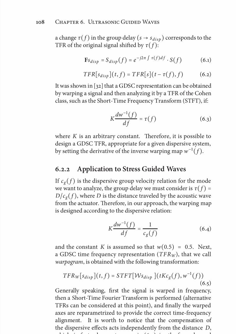
7/21/2019 Design and Computation of Warped Time-Frequency Transforms
http://slidepdf.com/reader/full/design-and-computation-of-warped-time-frequency-transforms 128/150
C . U G W
a change τ ( f ) in the group delay (s → sd i s p) corresponds to theTFR of the original signal shied by τ ( f ):
Fsd i s p = Sd i s p( f ) = e− jπ ∫ τ ( f )d f ⋅ S( f ) (.)
TFR[sd i s p](t , f ) = T FR[s](t − τ ( f ), f ) (.)
It was shown in [] that a GDSC representation can be obtainedby warping a signal and then analyzing it by a TFR of the Cohenclass, such as the Short-Time Frequency Transform (STFT), if:
K dw−
( f )d f = τ ( f ) (.)
where K is an arbitrary constant. erefore, it is possible todesign a GDSC TFR, appropriate for a given dispersive system,by setting the derivative of the inverse warping map w−( f ).
.. Application to Stress Guided Waves
If c g ( f ) is the dispersive group velocity relation for the modewe want to analyze, the group delay we must consider is τ ( f ) =Dc g ( f ), where D is the distance traveled by the acoustic wavefrom the actuator. erefore, in our approach, the warping mapis designed according to the dispersive relation:
K dw−
( f
)d f
=
c g ( f ) (.)
and the constant K is assumed so that w(.) = .. Next,a GDSC time frequency representation (TFRW ), that we call
warpogram, is obtained with the following transformation:
TFRW [sd i s p](t , f ) = STFT [W sd i s p ](tKc g ( f ), w−( f ))(.)
Generally speaking, first the signal is warped in frequency,then a Short-Time Fourier Transform is performed (alternativeTFRs can be considered at this point), and finally the warpedaxes are reparametrized to provide the correct time-frequency alignment. It is worth to notice that the compensation of the dispersive effects acts independently from the distance D,which, in facts, does not appear in (.), i.e. the formula usedfor map design.
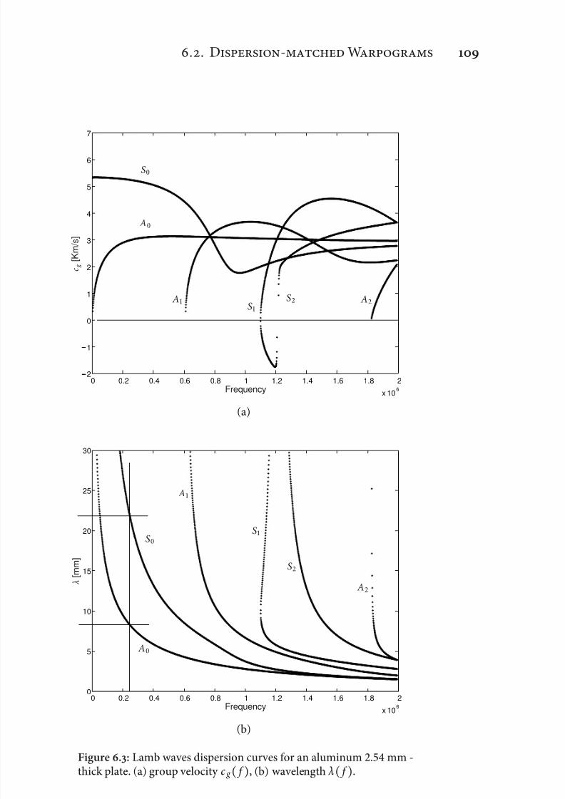
7/21/2019 Design and Computation of Warped Time-Frequency Transforms
http://slidepdf.com/reader/full/design-and-computation-of-warped-time-frequency-transforms 129/150
.. D- W
0 0.2 0.4 0.6 0.8 1 1.2 1.4 1.6 1.8 2
x 106
2
1
0
1
2
3
4
5
6
7
Frequency
c g
[ K m / s ]
A
S
AS
AS
(a)
0 0.2 0.4 0.6 0.8 1 1.2 1.4 1.6 1.8 2x 10
6
0
5
10
15
20
25
30
Frequency
λ
[ m m ]
A
S
A
S
A
S
(b)
Figure .: Lamb waves dispersion curves for an aluminum . mm -thick plate. (a) group velocity c g ( f ), (b) wavelength λ( f ).
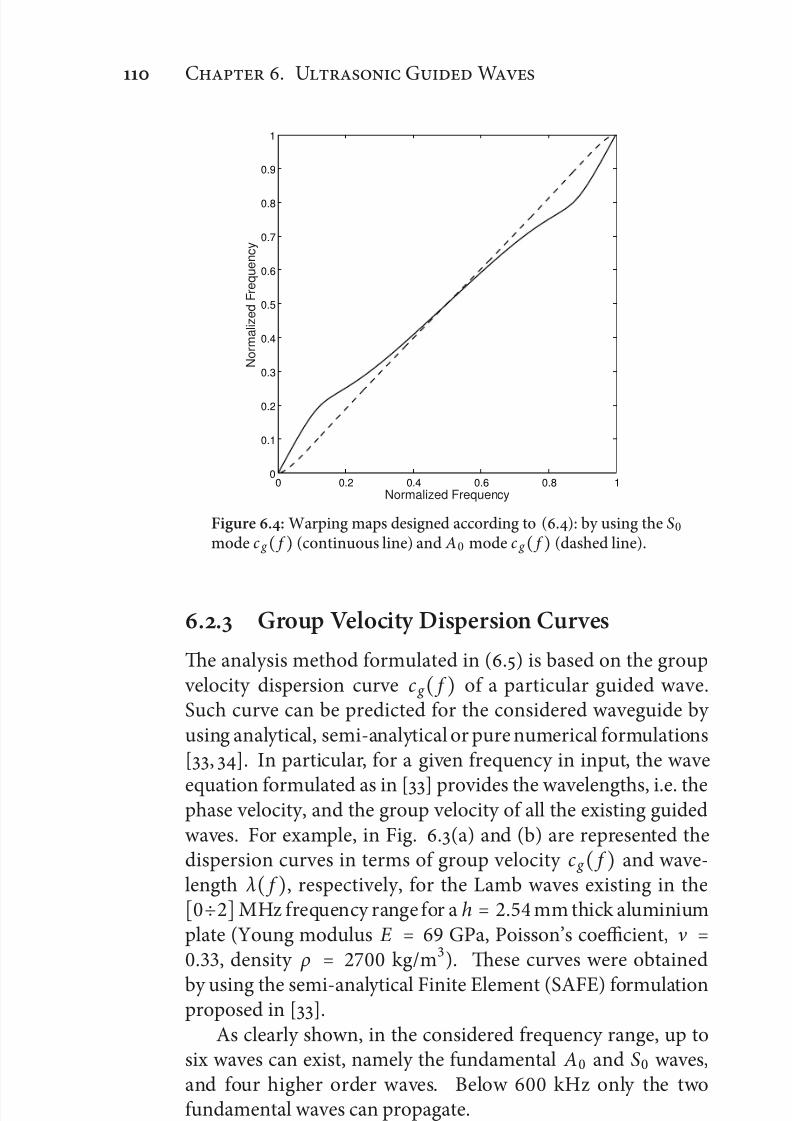
7/21/2019 Design and Computation of Warped Time-Frequency Transforms
http://slidepdf.com/reader/full/design-and-computation-of-warped-time-frequency-transforms 130/150
C . U G W
0 0.2 0.4 0.6 0.8 10
0.1
0.2
0.3
0.4
0.5
0.6
0.7
0.8
0.9
1
Normalized Frequency
N o r m a l i z e d F r e q u e n c y
Figure .: Warping maps designed according to (.): by using the S
mode c g ( f ) (continuous line) and A mode c g ( f ) (dashed line).
.. Group Velocity Dispersion Curves
e analysis method formulated in (.) is based on the group velocity dispersion curve c g ( f ) of a particular guided wave.Such curve can be predicted for the considered waveguide by using analytical, semi-analytical or pure numerical formulations[, ]. In particular, for a given frequency in input, the wave
equation formulated as in [] provides the wavelengths, i.e. thephase velocity, and the group velocity of all the existing guidedwaves. For example, in Fig. .(a) and (b) are represented thedispersion curves in terms of group velocity c g ( f ) and wave-length λ( f ), respectively, for the Lamb waves existing in the[÷]MHz frequency range for a h = . mm thick aluminiumplate (Young modulus E = GPa, Poisson’s coefficient, ν =., density ρ = kg/m). ese curves were obtained
by using the semi-analytical Finite Element (SAFE) formulationproposed in [].
As clearly shown, in the considered frequency range, up tosix waves can exist, namely the fundamental A and S waves,and four higher order waves. Below kHz only the twofundamental waves can propagate.

7/21/2019 Design and Computation of Warped Time-Frequency Transforms
http://slidepdf.com/reader/full/design-and-computation-of-warped-time-frequency-transforms 131/150
.. D- W
0 1 2 3 4 5 6
x 10−5
0
0.2
0.4
0.6
0.8
1
1.2
1.4
1.6
1.8
2x 10
6
Time
F r e q u e n c y
(a)
0 1 2 3 4 5 6
x 10
−5
0
0.2
0.4
0.6
0.8
1
1.2
1.4
1.6
1.8
2x 10
6
Time
F r e q u
e n c y
(b)
Figure .: Tiling of the time-frequency plane produced by usingthe warping map designed on the S group velocity dispersion curve(continuous line of Fig. .) and on the A group velocity dispersioncurve (dashed line of Fig. .).

7/21/2019 Design and Computation of Warped Time-Frequency Transforms
http://slidepdf.com/reader/full/design-and-computation-of-warped-time-frequency-transforms 132/150
C . U G W
.. Warping maps and Warpograms
e predicted c g
( f
) branches are used to design the warping
maps according to Eq. (.). In Fig. ., where these maps forthe A and S are plotted, it can be seen that just a slight bendingof the frequency axis is required.
In Fig. .(a) the tiling of the time-frequency plane shapedaccording to the warping map for the S wave (continuous linein Fig. .), is presented. It is worth noting how the atomsinclination varies in frequency following closely the mode dis-persive behavior. is guarantees to the warpogram enhancedsparsify if compared to the others TFRs. In addition, the atomschange their shape versus time in agreement to the dispersiveproperties of the mode as clearly visible in Fig. .(a) for adistance source-receiver of mm (continuous line) and mm (dashed line). is allows to the warpogram the desiredgroup covariant property. Similar considerations can be drawnon the tiling built on the A mode warping map (dashed line inFig. .) shown in Fig. .(b).
A case study on the signal sd i s p , represented in Fig. .(a)and Fig. .(a), is proposed. is signal was generated syntheti-cally by imposing the group delay shi of the modes depictedin Fig. . to a Dirac Delta. In Fig. . are shown the stepsused to obtain the Warpogram of sd i s p tuned on the S mode.e warping effect can be clearly seen in Fig. .(b). Roughly speaking, a guided wave whitin a signal is approximatively re-
converted into the incipient pulse (i.e. the Dirac Delta) at adistance from the origin which is proportional to the distancetraveled by the mode, thus compensating the mode dispersivebehavior. For instance, the two delta in Fig. .(b) correspondto the S mode at mm distance (continuous line in Fig. .)and at mm distance (dashed line in Fig. .), respectively.is important effect can be also fruitfully exploited for defectlocalization procedures []. Processing the signal
W sd i s p with
the STFT yields the Fig. .(c) that is next converted to thewarpogram of Fig. .(d) by reparametrizing the axes to providethe corred time frequency alignment. As it can be seen from Fig..(d) the WFT produces a sparse representation of the acquiredsignals. It is worth to notice that the mode acquired repeatedly issparsely represented in both cases (as warpograms are GDSC).Similar considerations can be made for the Warpogram tunedon the mode A, for the dispersive signal sd i s p , in Fig. .(d).
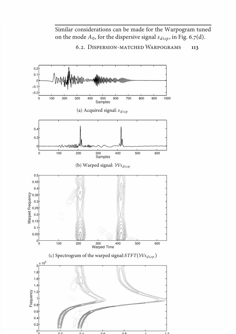
7/21/2019 Design and Computation of Warped Time-Frequency Transforms
http://slidepdf.com/reader/full/design-and-computation-of-warped-time-frequency-transforms 133/150
.. D- W
0 100 200 300 400 500 600 700 800 900 1000
−0.2
−0.1
0
0.1
0.2
Samples
(a) Acquired signal: sd i s p
0 100 200 300 400 500 600
0
0.2
0.4
Samples
(b) Warped signal: W sd i s p
0 100 200 300 400 500 6000
0.05
0.1
0.15
0.2
0.25
0.3
0.35
0.4
0.45
0.5
Warped Time
W a r p e d F r e q u e n c y
(c) Spectrogram of the warped signal:STFT (W sd i s p)
0 0.2 0.4 0.6 0.8 1 1.2
x 10−4
0
0.2
0.4
0.6
0.8
1
1.2
1.4
1.6
1.8
2x 10
6
Time
F r e q u e n c y
(d) Warpogram: STFT (W sd i s p )(tK c g ( f ), w −( f ))
Figure .: Warpogram calculation steps as described in Section ...e depicted Warpogram is calibrated to extract the S mode from thesynthetic signal of Fig. ..

7/21/2019 Design and Computation of Warped Time-Frequency Transforms
http://slidepdf.com/reader/full/design-and-computation-of-warped-time-frequency-transforms 134/150
C . U G W
0 100 200 300 400 500 600 700 800 900 1000
−0.2
−0.1
0
0.1
0.2
Samples
(a) Acquired signal: s d i s p
0 100 200 300 400 500 600−0.4
−0.2
0
0.2
0.4
Samples
(b) Warped signal: W sd i s p
0 100 200 300 400 500 6000
0.05
0.1
0.15
0.2
0.25
0.3
0.35
0.4
0.45
0.5
Warped Time
W a r p e d F r e q u e n c y
(c) Spectrogram of the warped signal: STFT (W sd i s p)
0 0.2 0.4 0.6 0.8 1 1.2
x 10−4
0
0.2
0.4
0.6
0.8
1
1.2
1.4
1.6
1.8
2x 10
6
Time
F r e q u e n c y
(d) Warpogram: STFT (W sd i s p )(tKc g ( f ), w −( f ))
Figure .: Warpogram calculation steps as described in Section ...e depicted Warpogram is calibrated to extract the A mode from thesynthetic signal of Fig. ..
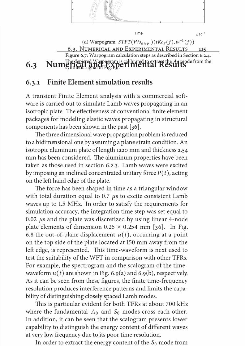
7/21/2019 Design and Computation of Warped Time-Frequency Transforms
http://slidepdf.com/reader/full/design-and-computation-of-warped-time-frequency-transforms 135/150
.. N E R
. Numerical and Experimental Results
.. Finite Element simulation results
A transient Finite Element analysis with a commercial so-ware is carried out to simulate Lamb waves propagating in anisotropic plate. e effectiveness of conventional finite elementpackages for modeling elastic waves propagating in structuralcomponents has been shown in the past [].
e three dimensional wave propagation problem is reducedto a bidimensional one by assuming a plane strain condition. Anisotropic aluminum plate of length mm and thickness .mm has been considered. e aluminum properties have beentaken as those used in section ... Lamb waves were excitedby imposing an inclined concentrated unitary force P (t ), actingon the le hand edge of the plate.
e force has been shaped in time as a triangular window with total duration equal to . µs to excite consistent Lambwaves up to . MHz. In order to satisfy the requirements forsimulation accuracy, the integration time step was set equal to. µs and the plate was discretized by using linear -nodeplate elements of dimension . × . mm []. In Fig.. the out-of-plane displacement u(t ), occurring at a pointon the top side of the plate located at mm away from thele edge, is represented. is time-waveform is next used totest the suitability of the WFT in comparison with other TFRs.
For example, the spectrogram and the scalogram of the time-waveform u(t ) are shown in Fig. .(a) and .(b), respectively.As it can be seen from these figures, the finite time-frequency resolution produces interference patterns and limits the capa-bility of distinguishing closely spaced Lamb modes.
is is particular evident for both TFRs at about kHzwhere the fundamental A and S modes cross each other.In addition, it can be seen that the scalogram presents lower
capability to distinguish the energy content of different wavesat very low frequency due to its poor time resolution.In order to extract the energy content of the S mode from
the signal u(t ) via the proposed WFT, first the warping mapmust be set. Next, the application of Eq. (.) gives the war-pogram tuned on the S mode as represented in Fig. .(c). Itcan be seen from this figure that the S mode is well captured allover the excited frequency range, while the A mode, as desired,
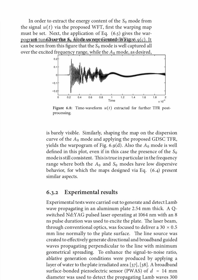
7/21/2019 Design and Computation of Warped Time-Frequency Transforms
http://slidepdf.com/reader/full/design-and-computation-of-warped-time-frequency-transforms 136/150
C . U G W
0 0.2 0.4 0.6 0.8 1 1.2 1.4 1.6 1.8 2
x 10
0.2
0.1
0
0.1
0.2
Time
Figure .: Time-waveform u(t ) extracted for further TFR post-processing.
is barely visible. Similarly, shaping the map on the dispersioncurve of the A mode and applying the proposed GDSC TFR,yields the warpogram of Fig. .(d). Also the A mode is welldefined in this plot, even if in this case the presence of the S
mode is still consistent. is is true in particular in the frequency range where both the A and S modes have low dispersive
behavior, for which the maps designed via Eq. (.) presentsimilar aspects.
.. Experimental results
Experimental tests were carried out to generate and detect Lambwave propagating in an aluminum plate . mm thick. A Q-
switched Nd:YAG pulsed laser operating at nm with an ns pulse duration was used to excite the plate. e laser beam,through conventional optics, was focused to deliver a × .mm line normally to the plate surface. e line source wascreated to effectively generate directional and broadband guidedwaves propagating perpendicular to the line with minimumgeometrical spreading. To enhance the signal-to-noise ratio,ablative generation conditions were produced by applying a
layer of water to the plate irradiated area [], []. A broadbandsurface-bonded piezoelectric sensor (PWAS) of d = mmdiameter was used to detect the propagating Lamb waves mm away from the illuminated spot. e ultrasonic signals wereamplified by using Panametrics pre-amp set at dB connectedto an oscilloscope and sampled at MHz. In Fig. .(a) and.(b) the spectrogram and the scalogram of the experimentalsignal are shown, respectively. Instead, in Fig. .(c) and
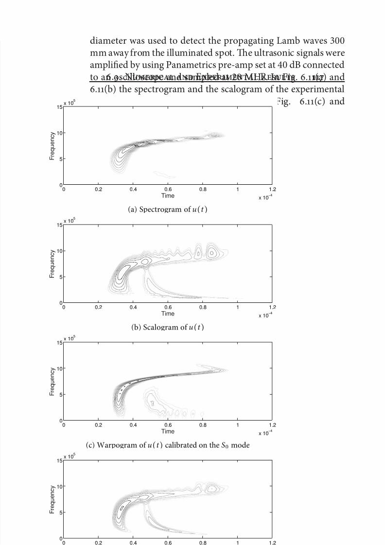
7/21/2019 Design and Computation of Warped Time-Frequency Transforms
http://slidepdf.com/reader/full/design-and-computation-of-warped-time-frequency-transforms 137/150
.. N E R
0 0.2 0.4 0.6 0.8 1 1.2
x 10−4
0
5
10
15x 10
5
Time
F r e q u e n c
y
(a) Spectrogram of u(t )
0 0.2 0.4 0.6 0.8 1 1.2
x 10−4
0
5
10
15x 10
5
Time
F r e q u e n c y
(b) Scalogram of u(t )
0 0.2 0.4 0.6 0.8 1 1.2
x 10−4
0
5
10
15x 10
5
Time
F r e q u e n c y
(c) Warpogram of u(t ) calibrated on the S mode
0 0.2 0.4 0.6 0.8 1 1.2
x 10−4
0
5
10
15x 10
5
Time
F r e q u e n c y
(d) Warpogram of u(t ) calibrated on the A mode
Figure .: Spectrogram, scalogram andwarpograms of the experimen-tal signal u(t ).
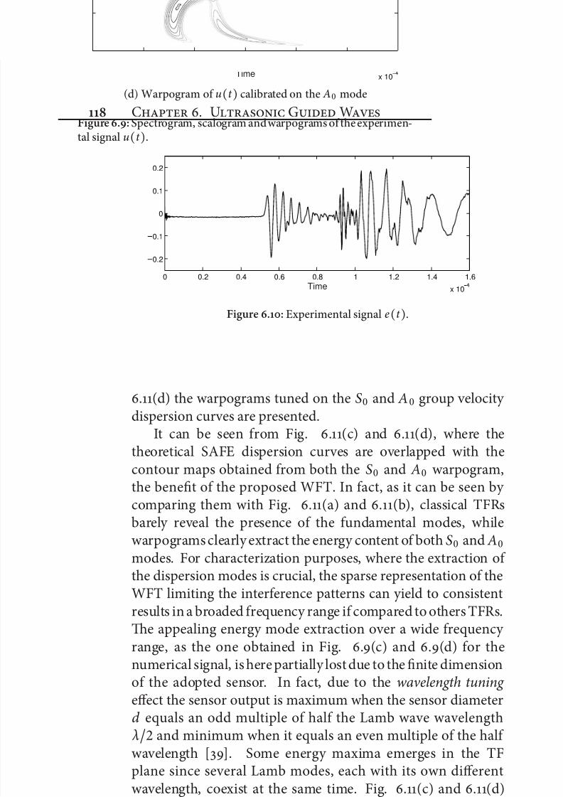
7/21/2019 Design and Computation of Warped Time-Frequency Transforms
http://slidepdf.com/reader/full/design-and-computation-of-warped-time-frequency-transforms 138/150
C . U G W
0 0.2 0.4 0.6 0.8 1 1.2 1.4 1.6
x 10
0.2
0.1
0
0.1
0.2
Time
Figure .: Experimental signal e(t ).
.(d) the warpograms tuned on the S and A group velocity dispersion curves are presented.
It can be seen from Fig. .(c) and .(d), where thetheoretical SAFE dispersion curves are overlapped with thecontour maps obtained from both the S and A warpogram,the benefit of the proposed WFT. In fact, as it can be seen by comparing them with Fig. .(a) and .(b), classical TFRsbarely reveal the presence of the fundamental modes, whilewarpograms clearly extract the energy content of both S and A
modes. For characterization purposes, where the extraction of the dispersion modes is crucial, the sparse representation of theWFT limiting the interference patterns can yield to consistent
results in a broaded frequency range if compared to others TFRs.e appealing energy mode extraction over a wide frequency range, as the one obtained in Fig. .(c) and .(d) for thenumerical signal, is here partially lost due to the finite dimensionof the adopted sensor. In fact, due to the wavelength tuning effect the sensor output is maximum when the sensor diameterd equals an odd multiple of half the Lamb wave wavelength λ
and minimum when it equals an even multiple of the half
wavelength []. Some energy maxima emerges in the TFplane since several Lamb modes, each with its own differentwavelength, coexist at the same time. Fig. .(c) and .(d)show the remarkable fact that, at kHz, the amplitude of the A mode goes through zero, while that of the S is close to itspeak. At this frequency, in fact, as it can be seen in Fig. .(b)the A mode has a wavelength around mm while the S modeapproximately mm.
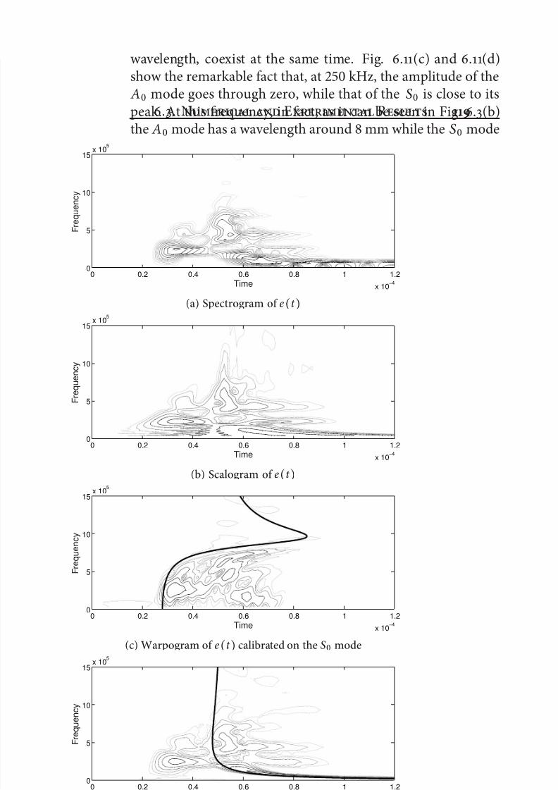
7/21/2019 Design and Computation of Warped Time-Frequency Transforms
http://slidepdf.com/reader/full/design-and-computation-of-warped-time-frequency-transforms 139/150
.. N E R
0 0.2 0.4 0.6 0.8 1 1.2
x 10−4
0
5
10
15x 10
5
Time
F r e q u e n c
y
(a) Spectrogram of e(t )
0 0.2 0.4 0.6 0.8 1 1.2
x 10−4
0
5
10
15x 10
5
Time
F r e q u e n c y
(b) Scalogram of e(t )
0 0.2 0.4 0.6 0.8 1 1.2
x 10−4
0
5
10
15x 10
5
Time
F r e q u e n c y
(c) Warpogram of e(t ) calibrated on the S mode
0 0.2 0.4 0.6 0.8 1 1.2
x 10−4
0
5
10
15x 10
5
Time
F r e q u e n c y
(d) Warpogram of e(t ) calibrated on the A mode
Figure .: Spectrogram, scalogram and warpograms of the experi-mental signal e(t ).
7/21/2019 Design and Computation of Warped Time-Frequency Transforms
http://slidepdf.com/reader/full/design-and-computation-of-warped-time-frequency-transforms 140/150
C . U G W
. Conclusions
In this chapter we presented a new TFR matched to the time-
frequency structures of Lamb waves. e new tool efficiently represents the different GWs with non-linearly frequency mod-ulated atoms. An application to propagating GWs in a singlelayer isotropic aluminum plate was presented to show the po-tential of the proposed procedure. Transient events obtainedfrom both dedicated finite element (FEM) simulations and ex-perimentally were considered to prove the reliability of the new tool. e main difference from the experimental numerical and
FEM based signals was due to the effect of a finite dimensiontransducer, revealing the so called wavelength tuning effect inthe experimental signals.
In general, the results showed that: i) the WFT produces asparser representation of a particular guided wave pattern thatcan be suitable for identification and characterization purposes;ii) the energy peaks extraction is a simpler task and can be per-formed to obtain reliable mode representation; iii) the quality
of the energy peaks extraction is independent on the distancewaves source - waves receiver, thanks to the group velocity covariant property. In conclusion the WFT thanks to its suitabletime-frequency support can be considered a powerful tool forthe analysis of dispersive systems.

7/21/2019 Design and Computation of Warped Time-Frequency Transforms
http://slidepdf.com/reader/full/design-and-computation-of-warped-time-frequency-transforms 141/150

7/21/2019 Design and Computation of Warped Time-Frequency Transforms
http://slidepdf.com/reader/full/design-and-computation-of-warped-time-frequency-transforms 142/150
7/21/2019 Design and Computation of Warped Time-Frequency Transforms
http://slidepdf.com/reader/full/design-and-computation-of-warped-time-frequency-transforms 143/150
7/21/2019 Design and Computation of Warped Time-Frequency Transforms
http://slidepdf.com/reader/full/design-and-computation-of-warped-time-frequency-transforms 144/150
C
pling operation. is algorithm has been theoretically andexperimentally shown to be effective in eliminating aliasing andincreasing the reconstruction accuracy.
Finally, a possible innovative application of warped time-frequency techniques has been shown. In particular, we focusedon the capability of frequency warping analysis techniques tomatch the physical characteristics of the propagation of guidedwaves. In fact, through the employment of frequency warpinga sparser representation of guided wave patterns have beenobtained, which can be usefully exploited for features extractionand propagation characterization.

7/21/2019 Design and Computation of Warped Time-Frequency Transforms
http://slidepdf.com/reader/full/design-and-computation-of-warped-time-frequency-transforms 145/150

7/21/2019 Design and Computation of Warped Time-Frequency Transforms
http://slidepdf.com/reader/full/design-and-computation-of-warped-time-frequency-transforms 146/150
7/21/2019 Design and Computation of Warped Time-Frequency Transforms
http://slidepdf.com/reader/full/design-and-computation-of-warped-time-frequency-transforms 147/150
Bibliography
[] B. de Smit and H. Lenstra Jr., “e mathematical structure
of escher’s print gallery,” NoticeoftheAMS, vol. , pp. –, .
[] M. Vetterli and J. Kovacevic, Wavelets and Subband Coding .Prentice Hall PTR, April .
[] G. Strang and T. Nguyen, Wavelets and Filter Banks.Wellesley College, .
[] A. Papandreou-Suppappola, R. Murray, B.-G. Iem, andG. Boudreaux-Bartels, “Group delay shi covariantquadratic time-frequency representations,” Signal Processing, IEEE Transactions on, vol. , no. , pp.–, Nov .
[] S. Franz, S. K. Mitra, and G. Doblinger, “Frequency es-timation using warped discrete fourier transform,” Signal
Processing , vol. , no. , pp. – , .[] R. Baraniuk and D. Jones, “Unitary equivalence: a new
twist on signal processing,” IEEE Trans. Signal Processing , vol. , no. , pp. –, .
[] G. Evangelista and S. Cavaliere, “Discrete frequency war-ped wavelets: theory and applications,” IEEE Trans. Signal Processing , vol. , no. , pp. –, .
7/21/2019 Design and Computation of Warped Time-Frequency Transforms
http://slidepdf.com/reader/full/design-and-computation-of-warped-time-frequency-transforms 148/150
B
[] G. Evangelista, “Dyadic warped wavelets,” Advances inImaging and Electron Physics, vol. , pp. –, .
[] A. Oppenheim and D. Johnson, “Discrete representation of signals,” Proc. IEEE, vol. , no. , pp. –, .
[] A. Makur and S. Mitra, “Warped discrete-fourier trans-form: eory and applications,” Circuits and Systems I:Fundamental eory and Applications, IEEE Transactionson, vol. , no. , pp. –, Sep .
[] U. Laine and T. Altosaar, “An orthogonal set of frequency and amplitude modulated (FAM) functions for variableresolution signal analysis,” in Proc. IEEE International Con-
ference on Acoustics, Speech, and Signal Processing , Albu-querque, NM, , pp. –.
[] A. Dutt and V. Rokhlin, “Fast fourier transforms for noneq-uispaced data,” SIAM Journal on Scientific Computing ,
vol. , no. , pp. –, .
[] Q. Liu and N. Nguyen, “An accurate algorithm for nonuni-form fast fourier transforms (NUFFT’s),” IEEE MicrowaveGuided Wave Lett., vol. , no. , pp. –, .
[] ——, “e regular Fourier matrices and nonuniform fastFourier transforms,” SIAM Journal on Scientific Computing , vol. , no. , pp. –, Jan. .
[] J. Fessler and B. Sutton, “Nonuniform fast fourier trans-forms using min-max interpolation,” IEEE Trans. Signal Processing , vol. , no. , pp. –, .
[] R. Duffin and A. Schaeffer, “A class of nonharmonic fourierseries,” Trans. Amer. Math. Soc., pp. Ű–, .
[] I. Daubechies, “e wavelet transform, time-frequency lo-calization and signal analysis,” IEEE Trans. Inform. eory , vol. , no. , pp. –, .
[] S. Caporale, L. De Marchi, and N. Speciale, “An accuratealgorithm for fast frequency warping,” in Proc. IEEE In-ternational Symposium on Circuits and Systems, , pp.–.
7/21/2019 Design and Computation of Warped Time-Frequency Transforms
http://slidepdf.com/reader/full/design-and-computation-of-warped-time-frequency-transforms 149/150
B
[] ——, “Analytical computation of fast frequency warping,”in Proc. IEEE International Conference on Acoustics, Speechand Signal Processing , , pp. –.
[] ——, “Fast operators for arbitrary warping maps,” in Proc.IEEE International Symposium on Circuits and Systems,.
[] ——, “A SVD-based algorithm for dense nonuniform fastfourier transform,” in Proc. EURASIP European Signal Pro-cessing Conference, , pp. –.
[] M. Do and M. Vetterli, “e contourlet transform: anefficient directional multiresolution image representation,”IEEE Trans. Image Processing , vol. , no. , pp. –,.
[] D. Alleyne and P. Cawley, “A two-dimensional Fouriertransform method for the measurement of propagating
multimode signals,” J. Acoust. Soc. Am., vol. , p. , .
[] W. Prosser, M. Seale, and B. Smith, “Time-frequency anal-ysis of the dispersion of Lamb modes,” e Journal of the
Acoustical Society of America, vol. , p. , .
[] A. Papoulis, Signal analysis. McGraw-Hill New York, .
[] M. Niethammer, L. Jacobs, J. Qu, and J. Jarrzynski, “Time-frequency representations of lamb waves,” J. Acoust. Soc.
Am., vol. (), pp. –, .
[] O. Kotte, M. Niethammer, and L. J. Jacobs, “Lamb wavecharacterization by differential reassignment and nonlin-ear anisotropic diffusion,” NDT & E International , vol. ,pp. –, .
[] S. Mallat and Z. Zhang, “Matching pursuits with time-frequency dictionaries,” IEEE Trans. Signal Process., vol. ,no. , pp. –, .
[] H. Kuttig, M. Niethammer, S. Hurlebaus, and L. J. Jacobs,“Model-based analysis of dispersion curves,” J. Acoust. Soc.
Am., vol. , pp. –, .
7/21/2019 Design and Computation of Warped Time-Frequency Transforms
http://slidepdf.com/reader/full/design-and-computation-of-warped-time-frequency-transforms 150/150
B
[] A. Raghavan and C. Cesnik, “Guided-wave signal process-ing using chirplet matching pursuits and mode correlationfor structural health monitoring,” Smart Materials and
Structures, vol. , no. , p. , .
[] T. Claasen and W. Mecklenbrauker, “e Wigner distribu-tionŮa tool for time-frequency signal analysis. II. Discretetime signals,” Philips Jl Research, vol. , pp. –, .
[] A. Papandreou-Suppappola, R. Murray, B. Iem, and G. F.Boudreaux-Bartels, “Group delay shi covariant quadratictime-frequency representations,” IEEE Trans. Signal Pro-cess., vol. , no. , pp. –, .
[] I. Bartoli, A. Marzani, F. Lanza di Scalea, and E. Viola,“Modeling wave propagation in damped waveguides of arbitrary cross-section,” Journal of Sound and Vibration, vol. , pp. –, .
[] A. Marzani, “Time-transient response for ultrasonic
guided waves propagating in damped cylinders,” Interna-tional Journal of Solids and Structures, vol. , no. -,pp. – , .
[] L. De Marchi, A. Marzani, S. Caporale, and N. Speciale,“A defect localization procedure based on warped lambwaves,” in Accepted to Proc. International Symposium on