design and application of quincunx filter banksfrodo/publications/ychen_mascthesis.pdf · design...

Design and Application of Quincunx Filter Banksby

Yi ChenB.Eng., Tsinghua University, China, 2002

A Thesis Submitted in Partial Fulfillment of theRequirements for the Degree of

MASTER OF APPLIED SCIENCE

in the Department of Electrical and Computer Engineering

c©Yi Chen, 2006

University of Victoria

All rights reserved. This thesis may not be reproduced in whole or in part, by photocopy orother means, without the permission of the author.

ii

Design and Application of Quincunx Filter Banksby

Yi ChenB.Eng., Tsinghua University, China, 2002

Supervisory Committee

Dr. Michael D. Adams, (Department of Electrical and Computer Engineering)

Co-Supervisor

Dr. Wu-Sheng Lu, (Department of Electrical and Computer Engineering)

Co-Supervisor

Dr. Reinhard Illner, (Department of Mathematics and Statistics)

Outside Member

iii

Supervisory Committee

Dr. Michael D. Adams, (Department of Electrical and Computer Engineering)

Co-Supervisor

Dr. Wu-Sheng Lu, (Department of Electrical and Computer Engineering)

Co-Supervisor

Dr. Reinhard Illner, (Department of Mathematics and Statistics)

Outside Member

ABSTRACT

Quincunx filter banks are two-dimensional, two-channel, nonseparable filter banks. They are widely used

in many signal processing applications. In this thesis, we study the design and applications of quincunx filter

banks in the processing of two-dimensional digital signals.

Symmetric extension algorithms for quincunx filter banks are proposed. In the one-dimensional case,

symmetric extension is a commonly used technique to build nonexpansive transforms of finite-length se-

quences. We show how this technique can be extended to the nonseparable quincunx case. We consider three

types of quadrantally-symmetric linear-phase quincunx filter banks, and for each of these types we show

how nonexpansive transforms of two-dimensional sequencesdefined on arbitrary rectangular regions can be

constructed.

New optimization-based techniques are proposed for the design of high-performance quincunx filter

banks for the application of image coding. The new methods yield linear-phase perfect-reconstruction sys-

tems with high coding gain, good analysis/synthesis filter frequency responses, and certain prescribed vanish-

ing moment properties. We present examples of filter banks designed with these techniques and demonstrate

their efficiency for image coding relative to existing filterbanks. The best filter banks in our design examples

outperform other previously proposed quincunx filter banksin approximately 80% cases and sometimes even

outperform the well-known 9/7 filter bank from the JPEG-2000standard.

iv

Contents

Abstract iii

Table of Contents iv

List of Tables vii

List of Figures viii

List of Acronyms xi

1 Introduction 1

1.1 Quincunx Filter Banks . . . . . . . . . . . . . . . . . . . . . . . . . . . . .. . . . . . . . 1

1.2 Historical Perspective . . . . . . . . . . . . . . . . . . . . . . . . . . .. . . . . . . . . . . 2

1.3 Overview and Contribution of This Thesis . . . . . . . . . . . . .. . . . . . . . . . . . . . 3

2 Preliminaries 5

2.1 Overview . . . . . . . . . . . . . . . . . . . . . . . . . . . . . . . . . . . . . . . .. . . . 5

2.2 Notation and Terminology . . . . . . . . . . . . . . . . . . . . . . . . . .. . . . . . . . . 5

2.3 Multidimensional Multirate Systems . . . . . . . . . . . . . . . .. . . . . . . . . . . . . . 6

2.3.1 Multidimensional Signals . . . . . . . . . . . . . . . . . . . . . . .. . . . . . . . 7

2.3.2 Multirate Fundamentals . . . . . . . . . . . . . . . . . . . . . . . . .. . . . . . . 9

2.3.3 Uniformly Maximally Decimated Filter Banks . . . . . . . .. . . . . . . . . . . . 12

2.3.4 Quincunx Filter Banks . . . . . . . . . . . . . . . . . . . . . . . . . . .. . . . . . 15

2.3.5 Relation Between Filter Banks and Wavelet Systems . . .. . . . . . . . . . . . . . 18

2.3.6 Lifting Realization of Quincunx Filter Banks . . . . . . .. . . . . . . . . . . . . . 20

2.4 Image Coding . . . . . . . . . . . . . . . . . . . . . . . . . . . . . . . . . . . . .. . . . . 21

v

2.4.1 Subband Image Compression Systems . . . . . . . . . . . . . . . .. . . . . . . . . 23

2.4.2 Coding Gain . . . . . . . . . . . . . . . . . . . . . . . . . . . . . . . . . . . .. . 23

3 Symmetric Extension for Quincunx Filter Banks 25

3.1 Overview . . . . . . . . . . . . . . . . . . . . . . . . . . . . . . . . . . . . . . . .. . . . 25

3.2 Introduction . . . . . . . . . . . . . . . . . . . . . . . . . . . . . . . . . . . .. . . . . . . 25

3.3 Types of Symmetries . . . . . . . . . . . . . . . . . . . . . . . . . . . . . . .. . . . . . . 28

3.4 Mapping Scheme . . . . . . . . . . . . . . . . . . . . . . . . . . . . . . . . . . .. . . . . 32

3.5 Preservation of Symmetry and Periodicity . . . . . . . . . . . .. . . . . . . . . . . . . . . 33

3.6 Symmetric Extension Algorithm . . . . . . . . . . . . . . . . . . . . .. . . . . . . . . . . 40

3.6.1 Type-1 Symmetric Extension Algorithm . . . . . . . . . . . . .. . . . . . . . . . . 41



3.6.4 Type-4 PR Quincunx Filter Banks . . . . . . . . . . . . . . . . . . .. . . . . . . . 50

3.6.5 Octave-Band Decomposition . . . . . . . . . . . . . . . . . . . . . .. . . . . . . . 52

3.7 Summary . . . . . . . . . . . . . . . . . . . . . . . . . . . . . . . . . . . . . . . . .. . . 54

4 Optimal Design of Quincunx Filter Banks 56

4.1 Overview . . . . . . . . . . . . . . . . . . . . . . . . . . . . . . . . . . . . . . . .. . . . 56

4.2 Introduction . . . . . . . . . . . . . . . . . . . . . . . . . . . . . . . . . . . .. . . . . . . 56

4.3 Lifting Parametrization of Linear-Phase PR Quincunx Filter Banks . . . . . . . . . . . . . . 57

4.3.1 Type-1 Filter Banks . . . . . . . . . . . . . . . . . . . . . . . . . . . . .. . . . . . 58

4.3.2 Type-2 and Type-3 Filter Banks . . . . . . . . . . . . . . . . . . . .. . . . . . . . 62

4.4 Design of Type-1 Filter Banks with Two Lifting Steps . . . .. . . . . . . . . . . . . . . . . 64

4.4.1 Coding Gain . . . . . . . . . . . . . . . . . . . . . . . . . . . . . . . . . . . .. . 65

4.4.2 Vanishing Moments . . . . . . . . . . . . . . . . . . . . . . . . . . . . . .. . . . 65

4.4.3 Frequency Response . . . . . . . . . . . . . . . . . . . . . . . . . . . . .. . . . . 70

4.4.4 Design Problem Formulation . . . . . . . . . . . . . . . . . . . . . .. . . . . . . . 73

4.4.5 Design Algorithm with Hessian . . . . . . . . . . . . . . . . . . . .. . . . . . . . 77

4.5 Design of Type-1 Filter Banks with More Than Two Lifting Steps . . . . . . . . . . . . . . 78

4.5.1 Vanishing Moments . . . . . . . . . . . . . . . . . . . . . . . . . . . . . .. . . . 79

4.5.2 Frequency Responses . . . . . . . . . . . . . . . . . . . . . . . . . . . .. . . . . . 81

4.5.3 Design Problem Formulation . . . . . . . . . . . . . . . . . . . . . .. . . . . . . . 82

vi

4.6 Suboptimal Design Algorithm . . . . . . . . . . . . . . . . . . . . . . .. . . . . . . . . . 86

4.7 Design Examples . . . . . . . . . . . . . . . . . . . . . . . . . . . . . . . . . .. . . . . . 87

4.8 Image Coding Results and Analysis . . . . . . . . . . . . . . . . . . .. . . . . . . . . . . 92

4.9 Summary . . . . . . . . . . . . . . . . . . . . . . . . . . . . . . . . . . . . . . . . .. . . 106

5 Conclusions and Future Research 108

5.1 Conclusions . . . . . . . . . . . . . . . . . . . . . . . . . . . . . . . . . . . . .. . . . . . 108

5.2 Future Research . . . . . . . . . . . . . . . . . . . . . . . . . . . . . . . . . .. . . . . . . 109

Bibliography 110

vii

List of Tables

3.1 Four types of quadrantal centrosymmetry . . . . . . . . . . . . .. . . . . . . . . . . . . . 29

3.2 Symmetry type forx′ wherex′[nnn] = (−1)|nnn|x[nnn] andX′(zzz) = X(−zzz) . . . . . . . . . . . . . . 31

3.3 Properties of the extended sequences . . . . . . . . . . . . . . . .. . . . . . . . . . . . . . 33

3.4 Symmetry type ofy wherey = x∗h . . . . . . . . . . . . . . . . . . . . . . . . . . . . . . 36

4.1 Comparison of algorithms with linear and quadratic approximations . . . . . . . . . . . . . 79

4.2 Filter bank comparison . . . . . . . . . . . . . . . . . . . . . . . . . . . .. . . . . . . . . 88

4.3 Test images . . . . . . . . . . . . . . . . . . . . . . . . . . . . . . . . . . . . . .. . . . . 100

4.4 Lossy compression results for thefinger image . . . . . . . . . . . . . . . . . . . . . . . 103

4.5 Lossy compression results for thesar2 image . . . . . . . . . . . . . . . . . . . . . . . . . 103

4.6 Lossy compression results for thegold image . . . . . . . . . . . . . . . . . . . . . . . . . 104

finger

sar2

gold

viii

List of Figures

1.1 Frequency responses of a quincunx lowpass filter . . . . . . .. . . . . . . . . . . . . . . . 2

2.1 An MD digital filter . . . . . . . . . . . . . . . . . . . . . . . . . . . . . . . .. . . . . . . 8

2.2 A lattice onZ2 . . . . . . . . . . . . . . . . . . . . . . . . . . . . . . . . . . . . . . . . . 10

2.3 An MD downsampler . . . . . . . . . . . . . . . . . . . . . . . . . . . . . . . . .. . . . . 10

2.4 An MD upsampler . . . . . . . . . . . . . . . . . . . . . . . . . . . . . . . . . . .. . . . 11

2.5 Cascade connection . . . . . . . . . . . . . . . . . . . . . . . . . . . . . . .. . . . . . . . 11

2.6 Noble identities . . . . . . . . . . . . . . . . . . . . . . . . . . . . . . . . .. . . . . . . . 12

2.7 A UMD filter bank . . . . . . . . . . . . . . . . . . . . . . . . . . . . . . . . . . .. . . . 13

2.8 Polyphase representation of a UMD filter bank before simplification with the noble identities 14

2.9 Polyphase representation of a UMD filter bank . . . . . . . . . .. . . . . . . . . . . . . . 14

2.10 Quincunx lattice . . . . . . . . . . . . . . . . . . . . . . . . . . . . . . . .. . . . . . . . . 15

2.11 Quincunx filter bank . . . . . . . . . . . . . . . . . . . . . . . . . . . . . .. . . . . . . . 16

2.12 Ideal frequency responses of quincunx filter banks . . . .. . . . . . . . . . . . . . . . . . . 16

2.13 AnN-level octave-band filter bank . . . . . . . . . . . . . . . . . . . . . . . . .. . . . . . 17

2.14 Frequency decomposition associated with octave-bandquincunx scheme . . . . . . . . . . . 17

2.15 The equivalent filter bank to octave-band . . . . . . . . . . . .. . . . . . . . . . . . . . . . 18

2.16 Lifting realization . . . . . . . . . . . . . . . . . . . . . . . . . . . . .. . . . . . . . . . . 21

2.17 Lifting realization of ITI transforms . . . . . . . . . . . . . .. . . . . . . . . . . . . . . . 22

2.18 Block diagram of an image coder . . . . . . . . . . . . . . . . . . . . .. . . . . . . . . . . 24

3.1 Filter bank with symmetric extension . . . . . . . . . . . . . . . .. . . . . . . . . . . . . . 27

3.2 1D symmetric extension . . . . . . . . . . . . . . . . . . . . . . . . . . . .. . . . . . . . 27

3.3 Quadrantal centrosymmetry . . . . . . . . . . . . . . . . . . . . . . . .. . . . . . . . . . . 29

ix

3.4 Rotated quadrantal centrosymmetry . . . . . . . . . . . . . . . . .. . . . . . . . . . . . . 31

3.5 Symmetric extension example . . . . . . . . . . . . . . . . . . . . . . .. . . . . . . . . . 34

3.6 Frequency responses of a type-1 filter bank . . . . . . . . . . . .. . . . . . . . . . . . . . 44

3.7 Scaling and wavelet functions for a type-1 filter bank . . .. . . . . . . . . . . . . . . . . . 44

3.8 Sequences in the type-1 filter bank . . . . . . . . . . . . . . . . . . .. . . . . . . . . . . . 45

3.9 Frequency responses of the Haar-like filter bank . . . . . . .. . . . . . . . . . . . . . . . . 48

3.10 Scaling and wavelet functions for the Haar-like filter bank . . . . . . . . . . . . . . . . . . . 48

3.11 Sequences in the Haar-like filter bank . . . . . . . . . . . . . . .. . . . . . . . . . . . . . 49

3.12 2-level symmetric extension . . . . . . . . . . . . . . . . . . . . . .. . . . . . . . . . . . 53

4.1 Analysis side of a quincunx filter bank . . . . . . . . . . . . . . . .. . . . . . . . . . . . . 58

4.2 Lifting realization . . . . . . . . . . . . . . . . . . . . . . . . . . . . . .. . . . . . . . . . 58

4.3 A quincunx filter bank with two lifting steps . . . . . . . . . . .. . . . . . . . . . . . . . . 65

4.4 Ideal frequency responses of quincunx filter banks . . . . .. . . . . . . . . . . . . . . . . . 71

4.5 Weighting function . . . . . . . . . . . . . . . . . . . . . . . . . . . . . . .. . . . . . . . 72

4.6 Lifting filter coefficients for (a) OPT1, (b) OPT2, and (c)OPT3. . . . . . . . . . . . . . . . 89

4.7 Lifting filter coefficients for (d) OPT4, (e) OPT5, and (f)OPT6. . . . . . . . . . . . . . . . 90

4.8 Lifting filter coefficients for OPT7. . . . . . . . . . . . . . . . . .. . . . . . . . . . . . . . 91

4.9 Frequency responses of OPT1 . . . . . . . . . . . . . . . . . . . . . . . .. . . . . . . . . 92

4.10 Scaling and wavelet functions for OPT1 . . . . . . . . . . . . . .. . . . . . . . . . . . . . 93

4.11 Frequency responses of OPT2 . . . . . . . . . . . . . . . . . . . . . . .. . . . . . . . . . 93

4.12 Scaling and wavelet functions for the OPT2 . . . . . . . . . . .. . . . . . . . . . . . . . . 94











4.23 Frequency responses of type2 filter bank . . . . . . . . . . . . .. . . . . . . . . . . . . . . 99

x

4.24 Scaling and wavelet functions for the type2 filter bank .. . . . . . . . . . . . . . . . . . . . 100

4.25 The finger image . . . . . . . . . . . . . . . . . . . . . . . . . . . . . . . . . .. . . . . . 101

4.26 The sar2 image . . . . . . . . . . . . . . . . . . . . . . . . . . . . . . . . . . .. . . . . . 101

4.27 The gold image . . . . . . . . . . . . . . . . . . . . . . . . . . . . . . . . . . .. . . . . . 102

4.28 Reconstructed images for the fingerprint image . . . . . . .. . . . . . . . . . . . . . . . . 105

4.29 Reconstructed images for the fingerprint image . . . . . . .. . . . . . . . . . . . . . . . . 107

xi

List of Acronyms

1D One-dimensional

2D Two-dimensional

CR Compression ratio

HVS Human visual system

ITI Integer-to-integer

LTI Linear time-invariant

MD Multidimensional

MRA Multiresolution approximation

MSE Mean-squared error

PR (Shift-free) perfect reconstruction

PSNR Peak-signal-to-noise ratio

SOCP Second-order cone programming

SVD Singular value decomposition

UMD Uniformly maximally decimated

Chapter 1

Introduction

1.1 Quincunx Filter Banks

One-dimensional (1D) and multidimensional (MD) filter banks have proven to be a highly effective tool for

the processing of digital signals including speech, image,and video. Usually, the MD case is handled via

tensor product, i.e., the MD signal is decomposed into 1D signals and processed by 1D filter banks along

each dimension. Some of the more recent efforts concentrateon the nonseparable case, where nonseparable

sampling and filtering are employed [1, 2, 3, 4, 5, 6, 7, 8]. Thequincunx sampling scheme is the simplest

two-dimensional (2D) nonseparable sampling scheme. It is used in many signal processing applications,

such as the handling of images returned from remote sensors of satellites [5] and intraframe coding of HDTV

[1, 9]. In contrast to the separable case, the quincunx sampling scheme leads to a two-channel filter bank and

reduces the scale by a factor of√

2.

Although the implementation of quincunx filter banks has higher computational complexity than the

dyadic separable case, these filter banks offer several important advantages. Firstly, the quincunx filter bank

is a good match to the human visual system (HVS) [10]. The HVS has a higher sensitivity to changes in

the horizontal and vertical directions [11]. This is equivalent to saying that the HVS is more accurate in per-

ceiving high frequencies in the horizontal and vertical directions than along diagonals. Figure 1.1 shows the

frequency response of a typical quincunx lowpass filter, where the shaded and unshaded regions correspond

to the passband and stopband, respectively. With the diamond-shaped passband, this filter conserves hori-

zontal and vertical high frequencies, and cuts diagonal frequencies by half. In this way, the quincunx filter

bank well matches the HVS. Another advantage of quincunx filter banks is that there are more degrees of

2

ω1

ω0−π π

π

−π

0

Figure 1.1: Frequency responses of a quincunx lowpass filter. The shaded and unshaded regions represent

the passband and stopband, respectively.

freedom in the design of such filter banks. This may lead to filter banks with better performance for targeted

applications.

1.2 Historical Perspective

Although 1D filter banks have been well studied, in the MD case, many problems remain unsolved. Filter

banks are often defined to operate on signals of infinite extent. In practice, however, we frequently deal with

signals of finite extent. This leads to the well-known boundary problem that can arise whenever a finite-extent

signal is filtered. In the 1D case, several solutions have been proposed to solve this problem by extending

the finite-extent signal into a signal with infinite extent. Zero padding and periodic extension [12, 13, 14]

introduce sharp discontinuities in the extended signals, which cause distortion at edges of the reconstructed

signals. Symmetric extension [14, 15, 16] is the most commonly used solution to the boundary problem

in the 1D case. This extension scheme provides smooth extended signals and leads to desirable nonexpan-

sive transforms. In the MD case, symmetric extension is often applied to the signals separably along each

dimension.

For 1D filter banks, various design techniques have been successfully developed. In the nonseparable

MD case, however, far fewer effective methods have been proposed. Variable transformation methods are

commonly used for the design of MD filter banks. With such methods, a 1D prototype filter bank is designed

first. Then it is mapped into an MD filter bank by a change of variables. For example, the McClellan trans-

formation [17] has been used in several design approaches [18, 19, 20, 21]. In these designs, the frequency

responses of the 1D filters are mapped into MD frequency responses. Other design techniques have also been

proposed where a transformation is applied to the polyphasecomponents of the filters instead of the original

filter transfer functions [22, 5, 7, 23]. These transformation-based designs have the restriction that one cannot

3

explicitly control the shape of the MD frequency responses,while in some cases the transformed MD filter

banks can only achieve approximate perfect reconstruction. Direct optimization of the filter coefficients has

also been proposed [24, 2, 25], but because of the involvement of large numbers of variables and nonlinear,

nonconvex constraints, such optimization typically leadsto a very complicated system, which is often diffi-

cult to solve. Designs through the lifting framework [26, 27] have been proposed in [28, 6] for two-channel

MD filter banks with an arbitrary number of vanishing moments. With these methods, however, only interpo-

lating filter banks (i.e., filter banks with two lifting steps) are considered. Thus, good filter banks with more

lifting steps cannot be designed with these approaches.

1.3 Overview and Contribution of This Thesis

This thesis is primarily concerned with the design and application of quincunx filter banks. A symmetric ex-

tension algorithm is presented to build nonexpansive transforms associated with quincunx filter banks. Then

an optimization-based design algorithm with some variations is proposed for constructing quincunx filter

banks with a number of desirable characteristics. Finally,the optimally designed filter banks are compared to

some previously proposed ones in terms of their performancein image coding.

The remainder of this thesis is structured as follows. Chapter 2 introduces the background necessary to

understand this work. We begin by discussing the notationalconventions used herein. Then, we introduce

multidimensional multirate systems and filter banks, and examine in detail the quincunx filter banks, which

are of the most interest in this work. At last, we present somebasic concepts related to subband image coding.

In the 1D case, when processing signals with finite lengths, symmetric extension is a very useful algorithm

to handle the signal boundaries and build nonexpansive transforms for such signals. In Chapter 3, we show

how this technique can be extended to the 2D quincunx case. Tothis end, we first define four ways to

extend finite-extent 2D sequences to infinite-extent sequences with four-fold symmetry and periodicity. Then

we discuss how these properties can be preserved under nonseparable sampling and filtering. Finally, we

propose several symmetric extension algorithms for building nonexpansive transforms with quincunx filter

banks, and illustrate the algorithms with several examples.

Chapter 4 presents new optimal design algorithms for quincunx filter banks. We begin with a lifting

parametrization of quincunx filter banks such that all of thefilters have symmetric or antisymmetric linear

phase. Based on this parametrization, we further show how tobuild filter banks compatible with the symmet-

ric extension algorithms discussed in Chapter 3. Then an optimization-based design algorithm is proposed

for the design of quincunx filter banks with perfect reconstruction (PR), linear phase, high coding gain, good

4

frequency selectivity and prescribed numbers of vanishingmoments. We show how this complex design

problem can be formulated as a second-order cone programming (SOCP) problem. Several variations of the

proposed algorithm are also investigated. Design examplesare presented to demonstrate the effectiveness of

our proposed design method. At the end of this chapter, we examine the performance of the optimal filter

banks, as well as some existing filter banks, in an image coder, and comment on their coding performance.

The experimental results show that our new filter banks outperform the previously proposed quincunx filter

banks in most cases, and sometimes even outperform the 9/7 filter bank, which is considered to be one of the

very best in the literature.

Chapter 5 summarizes the results presented in this thesis and suggests some related topics for future

research.

5

Chapter 2

Preliminaries

2.1 Overview

In this chapter, we first explain some fundamental concepts related to this work. We begin with an introduc-

tion to the notation and terminology used herein. We then present some of the basic concepts on multirate

systems and filter banks in the MD case. We conclude the chapter by a brief discussion on subband image

coding.

2.2 Notation and Terminology

In this work, matrices and vectors are denoted by upper and lower case boldface letters, respectively. The

symbolsC, R, andZ denote the sets of complex numbers, real numbers, and integers, respectively. The

symbol j denotes√−1. Forc ∈ C, c∗ denotes the complex conjugate ofc. In R, (a,b), [a,b], and[a,b)

denote the open interval{x : a < x < b}, the closed interval{x : a≤ x ≤ b}, and the half-open half-closed

interval{x : a≤ x< b}, respectively. The symbolsZ∗, Z+, Z−, Zodd, andZevendenote the sets of nonnegative,

positive, negative, odd, and even integers, respectively.For a setSand a scalark, the notationkSdenotes the

set{ks}s∈S. If k∈Z+, Sk denotes thek-fold Cartesian product ofS, i.e.,Sk ={sss= [s0 s1 · · · sk−1]

T}

si∈S.

As an example,Z2 denotes the set of ordered pairs of integers. Furthermore, for ak×k matrixMMM,MMMSk denotes

the set{MMMsss}sss∈Sk. The difference of two setsA andB is denotedA\B and defined asA\B= {x : x∈A,x 6∈B}.

The symbols 000, 111 andIII are used to denote a vector/matrix of all zeros, all ones, andan identity matrix,

respectively, the dimensions of which should be clear from the context. In particular,IIIk denotes an identity

6

matrix of sizek× k for somek ∈ Z. The symbols 000k and 111k are used to denotek-dimensional vectors of all

zeros and ones, respectively, and 000k0×k1 and 111k0×k1 are used to denotek0×k1 matrices of all zeros and ones,

respectively. For two vectors/matricesuuu andvvv, uuu◦vvv denotes theSchur product (i.e., element-wise product)

of uuu andvvv. We writeuuu≥ vvv if every element inuuu is no less than its corresponding element invvv. The notations

uuu>vvv, uuu≤vvvanduuu<vvvare defined in a similar way. For twoD-dimensional vectorsnnn= [n0 n1 · · · nD−1]T

andzzz= [z0 z1 · · · zD−1]T , we define

|nnn| =D−1

∑i=0

ni and zzznnn =D−1

∏i=0

znii .

Furthermore, for aD×D matrixMMM = [mmm0 mmm1 · · · mmmD−1] with mmmk being thekth column ofMMM, we define

zzzMMM = [zzzmmm0 zzzmmm1 · · · zzzmmmD−1]T .

Note that|nnn| andzzznnn are scalars, whilezzzMMM is a vector. With these notations, it can be verified that(zzzMMM)nnn

= zzzMMMnnn

and(zzzMMM)LLL

= zzzMMMLLL. For matrix multiplication, we define the product notation as

N

∏k=M

AAAk =

AAANAAAN−1 · · ·AAAM+1AAAM for N ≥ M

AAANAAAN+1 · · ·AAAM−1AAAM for N < M.

For convenience, in the rest of this thesis a linear (or polynomial) function of the elements of a vectorxxx is

simply referred to as a linear (or polynomial) function ofxxx.

For a ∈ R, ⌊a⌋ denotes the greatest integer less than or equal toa, and⌈a⌉ denotes the least integer no

less thana. For anM×N matrixAAA with the(i, j)th element beingai, j , ⌊AAA⌋ and⌈AAA⌉ each denotes anM×N

matrix where the(i, j)th element is⌊ai, j⌋

and⌈ai, j⌉, respectively. Form,n∈ Z, we define themod function

as mod(m,n) = m−n⌊m/n⌋.

2.3 Multidimensional Multirate Systems

Multirate systems are very useful in processing digital signals. In this section, we explain the basic concepts

of multirate signal processing and extend them to the MD case. We begin with an introduction to MD signals

and filter banks, and then concentrate on the quincunx case. Next, we briefly comment on the relation between

quincunx filter banks and dyadic wavelet systems. Lastly, weintroduce the lifting scheme that can be used to

efficiently design and implement filter banks.

7

2.3.1 Multidimensional Signals

We first introduce the notions of MD signals and filters. AD-dimensional signalx is a sequence of real

numbers given by

x ={

x[nnn] ∈ R∣∣nnn∈ ZD } .

An element ofx is denoted either asx[nnn] or x[n0,n1, . . . ,nD−1] (whichever is more convenient), wherennn =

[n0 n1 · · · nD−1]T andni ∈ Z. If only a finite number ofx[nnn] are nonzero, the sequencex is said to have

finite support. For a nonsingular integer matrixPPP, if x[nnn] = x[nnn+PPPkkk] for all nnn,kkk ∈ ZD, the sequencex is

said to bePPP-periodic andPPP is called aperiodicity matrix . The Fourier transform ˆx(ωωω) of x and the inverse

Fourier transform of ˆx(ωωω) are defined as

x(ωωω) = ∑nnn∈ZD

x[nnn]e− jωωωTnnn and x[nnn] =1

(2π)D

∫

[−π ,π)Dx(ωωω)ejωωωTnnndωωω ,

respectively. Thez-transform ofx is defined as

X(zzz) = ∑nnn∈ZD

x[nnn]zzz−nnn.

For aD-dimensional FIR filter H, its impulse responseh is a finitely supported sequence defined onZD.

The transfer functionH(zzz) and frequency responseh(ωωω) of H are given by

H(zzz) = ∑nnn∈ZD

h[nnn]zzz−nnn and h(ωωω) = ∑nnn∈ZD

h[nnn]e− jωωωTnnn,

respectively. Figure 2.1 shows a linear time-invariant (LTI) system characterized by the transfer function

H(zzz). The output sequencey is computed by the convolution ofx andh as

y[nnn] = ∑kkk∈ZD

x[kkk]h[nnn−kkk]. (2.1)

The above input-output relation (2.1) is equivalent to ˆy(ωωω) = x(ωωω)h(ωωω) andY(zzz) = X(zzz)H(zzz) in the frequency

domain andz-domain, respectively.

For a 2D filter H, for convenience, we express its impulse responseh in the form of a matrixAAAh and

denote the relationship ofh andAAAh as

h[nnn] ∼AAAh. (2.2)

In AAAh, the element corresponding toh[0,0] is framed. For example, a filter H with impulse responseh[−1,0]=

1, h[−1,1] = 2, h[−1,2] = 3, h[0,0] = 4, h[0,1] = 5, andh[0,2] = 6 is denoted as

h[nnn] ∼

h[−1,2] h[0,2]

h[−1,1] h[0,1]

h[−1,0] h[0,0]

=

3 6

2 5

1 4

.

8

H(zzz)x[nnn] y[nnn]

Figure 2.1: An MD digital filter.

A D-dimensional filter H with impulse responseh is said to havelinear phase with group delayccc if, for

someccc∈ 12ZD andS∈ {−1,1},

h[nnn] = Sh[2ccc−nnn] for all nnn∈ ZD. (2.3)

The filter H is said to besymmetric if S= 1, andantisymmetric if S= −1. For a linear-phase filter H, its

transfer functionH(zzz) satisfiesH(zzz) = Szzz−2cccH(zzz−1), and its frequency response can be expressed as

h(ωωω) = ∑nnn∈ZD

h[nnn]e− jωωωTnnn = S ∑nnn∈ZD

h[2ccc−nnn]e− jωωωTnnn = S ∑nnn∈ZD

h[nnn]e− jωωωT (2ccc−nnn)

=12 ∑

nnn∈ZD

h[nnn][

e− jωωωTnnn +Se− jωωωT (2ccc−nnn)]

=12

e− jωωωTccc ∑nnn∈ZD

h[nnn][

e− jωωωT (nnn−ccc) +Se− jωωωT (ccc−nnn)]

=

e− jωωωTccc ∑nnn∈ZD h[nnn]cos[ωωωT (nnn−ccc)

]for S= 1

e− j(ωωωTccc+π/2)∑nnn∈ZD h[nnn]sin[ωωωT (nnn−ccc)

]for S= −1.

(2.4)

For the case withS= 1, we define thesigned amplitude responseha(ωωω) to beh(ωωω) without the exponential

factore− jωωωTccc, i.e.,

ha(ωωω) = ∑nnn∈ZD

h[nnn]cos[ωωωT (nnn−ccc)

]for S= 1. (2.5)

The quantityha(ωωω) determines the shape of the frequency response, and∣∣ha(ωωω)

∣∣ is equivalent to theampli-

tude responseof H.

The MD sequences that we have discussed above are all defined on theD-dimensional integer latticeZD.

In multirate systems, we often deal with sequences defined ona subset ofZD, called alattice, associated with

a generating matrixMMM. Below we introduce some fundamentals on lattices.

Let MMM = [mmm0 mmm1 · · · mmmD−1]T be aD×D nonsingular integer matrix withmmmk ∈ ZD being thekth

column ofMMM. SinceMMM is nonsingular, the set{mmmk} is linearly independent. The lattice LAT(MMM) is defined as

the set of all possible vectors that can be represented as integer linear combinations ofmmmk [29], i.e.,

LAT(MMM) =

{

xxx∈ ZD

∣∣∣∣∣xxx =

D−1

∑k=0

nkmmmk = MMMnnn,∀nnn = [n0 n1 . . . nD−1]T ∈ ZD

}

. (2.6)

Using the notation we introduced in Section 2.2, LAT(MMM) can be written asMMMZD. The matrixMMM is called a

generating matrix or sampling matrix of LAT(MMM), and its columns{mmmk} are called the basis vectors. Note

9

that the generating matrix for a lattice is not unique. Thesampling densityof LAT(MMM) is defined as

d =1

|detMMM| , (2.7)

which describes the number of lattice points in a unit volume.

Given a sampling matrixMMM, thefundamental parallelepiped, denoted as FPD(MMM), is defined as

FPD(MMM) ={xxx∈ RD

∣∣xxx = MMMααα,ααα ∈ [0,1)D} ,

where[0,1)D denotes theD-fold Cartesian product of the half-open half-closed interval [0,1). The finite

set of integer vectors contained in FPD(MMM) is denoted asN (MMM) andN (MMM) = FPD(MMM)⋂

ZD. Let nnn be an

arbitrary vector inZD, thennnn can be expressed as [20]

nnn = kkk+MMMmmm, (2.8)

wherekkk andmmm are unique vectors satisfyingkkk ∈ N (MMM) andmmm∈ ZD. For a given vectornnn and a matrixMMM,

we denote the unique vectorkkk satisfying (2.8) askkk = mod(nnn,MMM). A cosetof LAT(MMM) in ZD is the set of all

vectors of the form (2.8), wherekkk is fixed and called thecoset vectorof this coset. The number of distinct

cosets of LAT(MMM) is |detMMM|.Figure 2.2(a) shows a lattice with its fundamental parallelepiped and two basis vectorsmmm0 andmmm1. A

generating matrix of this lattice isMMM = [mmm0 mmm1] =[

1 12 −1

], and the sampling density is13. There are also other

matrices that generate this lattice, such as[

1 −12 1

]and

[2 11 −1

]. Figure 2.2(b) shows the|detMMM| = 3 distinct

cosets represented by symbols•, ◦, and×, which are associated with coset vectors[0 0]T , [1 1]T , and[1 0]T ,

respectively.

2.3.2 Multirate Fundamentals

In this part, we show the important multirate concepts for the MD case, including downsampling, upsampling

and polyphase decomposition of signals and filters. The basic building blocks of a multirate system are the

downsamplerandupsampler, which perform the operations of downsampling and upsampling, respectively.

Figure 2.3 shows a downsampler, where the inputx is downsampled by a nonsingular integer matrixMMM, and

the outputy is given by

y[nnn] = (↓MMM)x[nnn] = x[MMMnnn], (2.9)

that is, the outputy contains all samples on LAT(MMM). Through the downsampler, the sampling density is

reduced by a factor of|detMMM|. The Fourier transform ˆy(ωωω) of y can be written in terms of the Fourier

10

n0

n1

0

1

2

−2

−1

3

−3

1 2−2 −1 3−3

FPD(MMM)

mmm1

mmm0

××

××

××

××

××

××

×

××

×◦

◦◦

◦◦

◦

◦◦

◦◦

◦ ◦◦

◦◦

◦

n0

n1

0

1

2

−2

−1

3

−3

1 2−2 −1 3−3

(a) (b)

Figure 2.2: (a) A lattice with generating matrix[

1 12 −1

], and (b) its three distinct cosets.

↓ MMMx[nnn] y[nnn]

Figure 2.3: An MD downsampler.

transform ˆx(ωωω) of x. The relation is given by

y(ωωω) =1

|detMMM| ∑kkk∈N (MMMT )

x(MMM−T(ωωω −2πkkk)

).

Let X(zzz) andY(zzz) be thez-transforms ofx andy, respectively. Then, downsampling in thez-domain can be

expressed as

Y(zzz) =1

|detMMM| ∑kkk∈N (MMMT )

X(elelel ◦zzzMMM−1), (2.10)

whereelelel =[el0 el1 · · · elD−1

]Tandlll = [l0 l1 · · · lD−1]

T =(− j2πkkkTMMM−1

)T. In the frequency domain, the

spectrum of the downsampled signal is the average of|detMMM| shifted and stretched versions of the spectrum

of the original signal.

Figure 2.4 shows an upsampler, whereMMM is a nonsingular integer matrix. The outputy is given by

y[nnn] = (↑MMM)x[nnn] =

x[MMM−1nnn] if nnn∈ LAT(MMM)

0 otherwise.(2.11)

The input-output relation in the Fourier domain andz-domain are similar to the 1D case, and are given by

y(ωωω) = x(MMMTωωω

)and Y(zzz) = X

(zzzMMM) ,

11

↑ MMMx[nnn] y[nnn]

Figure 2.4: An MD upsampler.

↓ MMM1 ↓ MMM2

x[nnn] y[nnn]↓ (MMM1MMM2)

x[nnn] y[nnn]≡

(a)

↑ MMM1 ↑ MMM2

x[nnn] y[nnn]↑ (MMM2MMM1)

x[nnn] y[nnn]≡

(b)

Figure 2.5: Cascade connections and their equivalent formsof the (a) downsamplers and (b) upsamplers.

respectively. The upsampled signaly is nonzero only at points on the lattice LAT(MMM). In the frequency

domain, the upsampler performs a linear transformation of the frequency vectorωωω , and|detMMM| copies of the

original baseband spectrum are squeezed into the region[−π ,π)2.

Sometimes the downsamplers/upsamplers are applied in cascade. They can be combined as follows.

Figure 2.5(a) shows a cascade of two downsamplers with the downsampling matricesMMM1 andMMM2 and its

equivalent form with a single downsamplerMMM = MMM1MMM2. Figure 2.5(b) shows a cascade of two upsamplers

with MMM1 andMMM2 and its equivalent structure with a single upsamplerMMM = MMM2MMM1.

The downsampler and upsampler are often used in cascade withfilters. The order of the downsam-

pler/upsampler and the filter can be interchanged under certain circumstances. Figures 2.6(a) and (b) show

the equivalent structures for the downsampling and upsampling operations, respectively. They are called the

noble identities. With these identities, one can apply the convolution operation on the side of the downsampler

or upsampler with lower sampling density, which is very useful to improve the computation efficiency.

Now we consider the polyphase decomposition of MD signals and filters. From Section 2.3.1, we know

that an arbitrary MD integer vectornnn can be expressed uniquely in the form of (2.8). Therefore, given a

sequencex and a sampling matrixMMM, there areM = |detMMM| unique subsequences

xk[nnn] = x[MMMnnn+mmmk], (2.12)

for k = 0,1, . . . ,M − 1, mmmk ∈ N (MMM) and{mmmk} are distinct. The subsequencexk is called thekth type-1

polyphase componentof x. As xk[nnn] is theMMM-fold downsampled version ofx[nnn+mmmk], the sequencex can be

written as the sum of the upsampled and shifted versions of its polyphase components{xk} as

x[nnn] =M−1

∑k=0

((↑MMM)xkkk)[nnn−mmmk]. (2.13)

12

↓ MMM H(zzz)x[nnn] y[nnn]

↓ MMMH(zzzMMM )x[nnn] y[nnn]

≡

(a)

↑ MMM H(zzzMMM )x[nnn] y[nnn]

↑ MMMH(zzz)x[nnn] y[nnn]

≡

(b)

Figure 2.6: Noble identities of the (a) downsampler and (b) upsampler.

The above equation (2.13) is called thetype-1 polyphase representationof x. In the Fourier domain and

z-domain, (2.13) can be expressed as

x(ωωω) =M−1

∑k=0

e− jωωωTmmmkxk(MMMTω) and X(zzz) =

M−1

∑k=0

zzz−mmmkXk(zzzMMM) ,

respectively.

Similarly, we define thekth type-2 polyphase componentof a sequencex as

xk[nnn] = x[MMMnnn−mmmk], (2.14)

wherek ∈ {0,1, . . . ,M − 1}, mmmk ∈ N (MMM) and{mmmk} are distinct. The time domain, Fourier domain, and

z-domain expressions of the type-2 polyphase representation of a sequencex are respectively given by

x[nnn] =M−1

∑k=0

((↑MMM)xkkk)[nnn+mmmk],

x(ωωω) =M−1

∑k=0

ejωωωTmmmkxk(MMMT ω), and X(zzz) =

M−1

∑k=0

zzzmmmkXk(zzzMMM) .

2.3.3 Uniformly Maximally Decimated Filter Banks

The uniformly maximally decimated (UMD) filter bank is of great importance in multirate systems. The

block diagram of a UMD filter bank withM = |detMMM| channels is shown in Figure 2.7. On the analysis

side, the analysis filters{Hk} divide the input sequencex into subbands in theD-dimensional frequency

domain. The output of each analysis filter is then downsampled byMMM, yielding the subband sequences{yk}.

Since there areM analysis filters and each downsampler reduces the sampling density by a factor ofM, the

combined sampling rate of the subbands{yk} is the same as that of the inputx. On the synthesis side, the

subband sequences are upsampled byMMM, and then pass through the synthesis filters{Gk}. The outputs of the

synthesis filters are added together to obtain the reconstructed sequencexr . If xr [nnn] = x[nnn], the filter bank is

said to have theshift-free perfect reconstruction (PR) property. The shift-free PR property is desirable in

13

HM−1(zzz)

H0(zzz)

H1(zzz)

↓ MMM

↓ MMM

↓ MMM

↑ MMM

↑ MMM

↑ MMM GM−1(zzz)

G0(zzz)

G1(zzz)

+

+

......

......

......

x[nnn] xr[nnn]y0[nnn]

y1[nnn]

yM−1[nnn]

︸︷︷︸︸︷︷︸

analysis side synthesis side

Figure 2.7: AnM-channel UMD filter bank, whereM = |detMMM|.

many signal processing applications. In this thesis, henceforth, the term PR shall denote shift-free perfect

reconstruction unless explicitly noted otherwise.

With the polyphase representation introduced in Section 2.3.2, the UMD filter bank can also be imple-

mented in the polyphase domain. Each analysis filter Hk can be represented in the form of

Hk(zzz) =M−1

∑i=0

zzzmmmi Hk,i(zzzMMM) , (2.15)

whereHk,i (zzz) is theith type-2 polyphase component of Hk. The analysis filter transfer functions{Hk(zzz)} can

be written as

H0(zzz)

H1(zzz)...

HM−1(zzz)

=

H0,0(zzzMMM)

H0,1(zzzMMM)

· · · H0,M−1(zzzMMM)

H1,0(zzzMMM)

H1,1(zzzMMM)

· · · H1,M−1(zzzMMM)

......

. . ....

HM−1,0(zzzMMM)

HM−1,1(zzzMMM)

· · · HM−1,M−1(zzzMMM)

︸︷︷︸

HHH p(zzzMMM)

zzzmmm0

zzzmmm1

...

zzzmmmM−1

. (2.16)

The matrixHHH p(zzz) is called theanalysis polyphase matrix.

Similarly, the synthesis filter transfer functions{Gk(zzz)} can be written as

G0(zzz)

G1(zzz)...

GM−1(zzz)

=

G0,0(zzzMMM)

G0,1(zzzMMM)

· · · G0,M−1(zzzMMM)

G1,0(zzzMMM)

G1,1(zzzMMM)

· · · G1,M−1(zzzMMM)

......

. . ....

GM−1,0(zzzMMM)

GM−1,1(zzzMMM)

· · · GM−1,M−1(zzzMMM)

︸︷︷︸

GGGTp(zzzMMM)

zzz−mmm0

zzz−mmm1

...

zzz−mmmM−1

, (2.17)

14

HHHp(zzzMMM )

↓ MMM

↓ MMM

↓ MMM

zzzmmm0

zzzmmm1

zzzmmmM−1

GGGp(zzzMMM )

↑ MMM

↑ MMM

↑ MMM

zzz−mmm0

zzz−mmm1

zzz−mmmM−1

+

+

......

......

......

...

x[nnn] y0[nnn]

y1[nnn]

yM−1[nnn]

xr[nnn]

Figure 2.8: The polyphase representation of a UMD filter bankbefore simplification with the noble identities.

HHHp(zzz)

↓ MMM

↓ MMM

↓ MMM

zzzmmm0

zzzmmm1

zzzmmmM−1

GGGp(zzz)

↑ MMM

↑ MMM

↑ MMM

zzz−mmm0

zzz−mmm1

zzz−mmmM−1

+

+

......

......

......

...

x[nnn] y0[nnn]

y1[nnn]

yM−1[nnn]

xr[nnn]

Figure 2.9: The polyphase representation of a UMD filter bank.

whereGk,i(zzz) is theith type-1 polyphase component of the synthesis filter Gk, i.e.,Gk(zzz)= ∑M−1i=0 zzz−mmmkGk,i

(zzzMMM),

andGGGp(zzz) is called thesynthesis polyphase matrix. With (2.16) and (2.17), the filter bank can be imple-

mented in its polyphase domain as shown in Figure 2.8. Using the noble identities, we can interchange the

downsamplers/upsamplers and the polyphase matrices to obtain the simplified structure shown in Figure 2.9.

This structure provides a convenient way to design and implement UMD filter banks. In order for the filter

bank to have (shift-free) PR, the polyphase matrices must satisfy

HHH p(zzz)GGGp(zzz) = III . (2.18)

15

FPD(MMM)

0 1

1

n0

n1

Figure 2.10: The quincunx lattice.

2.3.4 Quincunx Filter Banks

The two-dimensional (2D)quincunx lattice is the simplest nonseparable lattice. Figure 2.10 shows the

quincunx lattice, where the symbols• and◦ represent the two distinct cosets associated with coset vectors

kkk0 = [0 0]T andkkk1 = [1 0]T , respectively. There are many matrices that generate the quincunx lattice, such as[

2 10 1

]and

[1 11 −1

]. Herein, we shall always choose the generating matrix to beMMM =

[1 11 −1

]. In this way, when

two downsamplers are cascaded, the equivalent single downsampling matrix becomes a separable diagonal

matrixMMM2 =[

2 00 2

].

With the quincunx downsampling matrixMMM =[

1 11 −1

], the downsampling operation, as shown in Fig-

ure 2.3, with input sequencex and output sequencey is expressed in time domain, Fourier domain, and

z-domain as

y[n0,n1] = x[n0 +n1,n0−n1],

y(ω0,ω1) =12

[

x(ω0+ω1

2 , ω0−ω12

)+ x(ω0+ω1

2 −π , ω0−ω12 −π

)]

, and

Y(z0,z1) =12

[

X(z120 z

121 ,z

120 z

− 12

1 )+X(−z120 z

121 ,−z

120 z

− 12

1 )

]

,

respectively. The upsampling operation shown in Figure 2.4is expressed in time domain, Fourier domain,

andz-domain as

y[n0,n1] =

x[1

2(n0 +n1),12(n0−n1)

]if [n0 n1]

T ∈ LAT(MMM)

0 otherwise,

y(ω0,ω1) = x(ω0 + ω1,ω0−ω1) , and Y(z0,z1) = X(z0z1,z0z−1

1

),

respectively.

Figure 2.11 shows a UMD filter bank based on quincunx sampling, whereMMM denotes the quincunx gen-

erating matrix[

1 11 −1

], {Hk} and{Gk} are the analysis and synthesis filters, respectively. The (shift-free) PR

16

H0(zzz)

H1(zzz)

↓ MMM

↓ MMM

↑ MMM

↑ MMM

G0(zzz)

G1(zzz)

+x[nnn] xr[nnn]y0[nnn]

y1[nnn]

Figure 2.11: A two-channel quincunx UMD filter bank.

ω1

ω0−π π

π

−π

0

ω1

ω0−π π

π

−π

0

(a) (b)

Figure 2.12: Ideal frequency responses of quincunx filter banks for the (a) lowpass filters and (b) highpass

filters.

condition for the quincunx UMD filter bank is

H0(zzz)G0(zzz)+H1(zzz)G1(zzz) = 2 and (2.19a)

H0(−zzz)G0(zzz)+H1(−zzz)G1(zzz) = 0, (2.19b)

where{Hk(zzz)} and{Gk(zzz)} are the analysis and synthesis filter transfer functions, respectively.

The quincunx lowpass and highpass filters are often chosen tohave diamond-shaped frequency responses

as shown in Figures 2.12(a) and (b), respectively. In these figures, passband and stopband are represented by

the shaded and unshaded areas, respectively. With the diamond-shaped frequency response, the lowpass filter

can preserve high frequencies in the horizontal and vertical directions, which is a good match to the human

visual system as the visual sensitivity is higher to changesin these two directions than in other directions.

In many image processing applications, a quincunx filter bank is typically applied in a recursive manner

in the lowpass channel, resulting in an octave-band filter bank structure as shown in Figure 2.13. With the

ideal frequency responses shown in Figure 2.12, this structure leads to a frequency decomposition shown in

Figure 2.14. For anN-level octave-band filter bank generated from a quincunx filter bank with analysis filters

{Hk}, by using the noble identities and combining cascaded downsamplers, upsamplers and filters, we obtain

the equivalent nonuniform filter bank shown in Figure 2.15. The equivalent filter bank hasN + 1 channels

17

H0(zzz)

H1(zzz)

↓ MMM

↓ MMM

H0(zzz)

H1(zzz)

↓ MMM

↓ MMM

H0(zzz)

H1(zzz)

↓ MMM

↓ MMM

x[nnn]· · · y0[nnn]

y1[nnn]

yN−1[nnn]

yN [nnn]

...

(a)

G0(zzz)

G1(zzz)

↑ MMM

↑ MMM

G0(zzz)

G1(zzz)

↑ MMM

↑ MMM

G0(zzz)

G1(zzz)

↑ MMM

↑ MMM

+++ xr[nnn]· · ·y0[nnn]

y1[nnn]

yN−1[nnn]

yN [nnn]

...

(b)

Figure 2.13: The structure of anN-level octave-band quincunx filter bank. (a) Analysis side and (b) synthesis

side.

ω0

ω1

−π π

π

−π

0

Figure 2.14: Frequency decomposition associated with octave-band quincunx scheme.

18

H ′

N (zzz) ↓ MMM G′

N (zzz)↑ MMM

H ′

N−1(zzz) ↓ MMM2 G′

N−1(zzz)↑ MMM2 +

H ′

1(zzz) ↓ MMMN G′

1(zzz)↑ MMMN +

H ′

0(zzz) ↓ MMMN G′

0(zzz)↑ MMMN +

...

x[nnn] y0[nnn]

y1[nnn]

yN−1[nnn]

yN [nnn]

xr[nnn]

......

......

......

Figure 2.15: The equivalent nonuniform filter bank associated with theN-level octave-band filter bank.

with analysis filters{H′i} and synthesis filters{G′

i}. The impulse responses of these equivalent filters can

be computed by iterative upsampling and convolution of the original analysis and synthesis filter impulse

responses as

h′i =

h0∗ (↑ M)h0∗ (↑ M2)h0∗ · · · ∗ (↑ MN−1)h0 for i = 0

h0∗ (↑ M)h0∗ · · · ∗ (↑ MN−i−1)h0∗ (↑ MN−i)h1 for 1≤ i ≤ N−1

h1 for i = N, and

(2.20)

g′i =

g0∗ (↑ M)g0∗ (↑ M2)g0∗ · · · ∗ (↑ MN−1)g0 for i = 0

g0∗ (↑ M)g0∗ · · · ∗ (↑ MN−i−1)g0∗ (↑ MN−i)g1 for 1≤ i ≤ N−1

g1 for i = N.

(2.21)

The transfer functions{H ′i (zzz)} of {H′

i} are given by

H ′i (zzz) =

∏N−1k=0 H0

(

zzzMMMk)

i = 0

H1

(

zzzMMMN−i)

∏N−i−1k=0 H0

(

zzzMMMk)

1≤ i ≤ N−1

H1 (zzz) i = N.

(2.22)

The transfer functions{G′i(zzz)} of the equivalent synthesis filters{G′

i} can be derived in a similar way.

2.3.5 Relation Between Filter Banks and Wavelet Systems

Filter banks and wavelets are closely connected [30]. Filter banks can be viewed as discrete wavelet trans-

forms [31], and continuous-time wavelet bases can be derived using iterated filter banks [32, 10]. Therefore,

when an octave-band filter bank is applied to a signal, the shape of the basis functions of the associated

19

wavelet may appear as artifacts in the reconstructed signalif the transformed coefficients are quantized. In

this section, we briefly explain how filter banks are related to wavelet systems in the quincunx case.

We consider the dyadic wavelet systems, where functions arerepresented at different resolutions where

successive resolution differs in scale by a factor of two. A wavelet system is a basis ofL2(R2)

derived

from amultiresolution approximation (MRA) [32]. Consider an MRA associated with scaling function φ

satisfying the refinement equation

φ(xxx) =√

2 ∑kkk∈Z2

c[kkk]φ(MMMxxx−kkk), (2.23)

and wavelet functionψ satisfying the wavelet equation

ψ(xxx) =√

2 ∑kkk∈Z2

d[kkk]φ(MMMxxx−kkk), (2.24)

whereMMM is the generating matrix of the quincunx lattice. Thedual MRA is associated with scaling function

φ and wavelet functionψ , whereφ andψ are the dual Riesz bases ofφ andψ , and satisfy the scaling and

wavelet equations

φ (xxx) =√

2 ∑kkk∈Z2

c[kkk]φ (MMMxxx−kkk) and ψ(xxx) =√

2 ∑kkk∈Z2

d[kkk]φ(MMMxxx−kkk),

respectively.

A quincunx UMD filter bank as the one shown in Figure 2.11 is related to the above MRA as

h0[nnn] = c∗[−nnn], h1[nnn] = d∗[−nnn], g0[nnn] = c[nnn], and g1[nnn] = d[nnn]. (2.25)

Therefore, the choice of filters determines the shape of the scaling and wavelet functions. Iteratively up-

sampling and convolving the lowpass analysis or synthesis filter produces a shape approximating the dual

or primal scaling function, respectively. Similarly, the shape of the wavelet function can be approximated

with a similar approach starting from the convolution of thelowpass and highpass filters followed by itera-

tive upsampling and convolution with the lowpass filter. Referring to theN-level octave-band quincunx filter

bank shown in Figure 2.13 and its equivalent form in Figure 2.15, the shape of the impulse responsesh′0[nnn]

andg′0[nnn] of the equivalent filters H′0 and G′0 approximate the shape of the dual and primal scaling func-

tions, respectively, and the shape ofh′i [nnn] andg′i [nnn] approximate that of the wavelet functions more and more

accurately asi decreases fromN to 1.

The number ofvanishing momentsis of interest herein. It corresponds to the highest order ofpolynomials

that can be reproduced by the scaling function. From the filter bank point of view, it represents the highpass

filter’s ability to annihilate polynomials. If there are a certain number of vanishing moments, and the original

20

signal can be well approximated by polynomials, then the highpass and bandpass subbands contain few

nonzero coefficients, which is favorable in many signal processing applications. The number of vanishing

moments is equivalent to the order of zero at[0 0]T in the highpass filter frequency response, or the order of

zero at[π π ]T in the lowpass filter frequency response. Similar to the sum rule in the 1D case, we have the

following lemma for the quincunx case.

Lemma 2.1 (Sum rule). Let c and d be sequences defined onZ2 with Fourier transformsc(ωωω) and d(ωωω),

respectively. Then,c(ωωω) has an Nth order zero atωωω = [π π ]T if and only if

∑nnn∈Z2

(−1)|nnn|nnnmmmc[nnn] = 0, for |mmm| < N, (2.26)

andd(ωωω) has an Nth order zero atωωω = [0 0]T if and only if

∑nnn∈Z2

nnnmmmd[nnn] = 0, for |mmm| < N. (2.27)

Therefore, for a UMD quincunx filter bank to haveN vanishing moments, the impulse response of the

corresponding lowpass or highpass filter is required to satisfy the linear system (2.26) or (2.27), respectively.

The presence of vanishing moments is desirable in many applications.

2.3.6 Lifting Realization of Quincunx Filter Banks

The lifting scheme[26, 27] is an efficient method used to design and implement filter banks. The lifting

structure provides a number of advantages over the traditional filter bank realization. It features fast and in-

place computation, satisfies the (shift-free) PR conditionautomatically, and can be used to construct reversible

integer-to-integer (ITI) transforms [33]. Unlike the 1D case, only a subset of all PR quincunx filter banks can

be implemented using the lifting scheme.

The lifting realization of a quincunx filter bank with 2λ lifting filters is shown in Figure 2.16. Without loss

of generality, we assume that none of the 2λ lifting filter transfer functions{Ak(zzz)} are identically zero, except

possiblyA1(zzz) andA2λ (zzz). With the lifting structure for the forward transform shownin Figure 2.16(a), the

input sequencex is decomposed into its two polyphase components, and then each lifting step adds a filtered

version of the sequence in one channel to the sequence in the other channel. The inverse transform has a

similar structure which undoes each step of the forward transform as shown in Figure 2.16(b). In this way,

the PR condition is satisfied structurally.

The analysis polyphase matrix can be derived from the lifting filters as

HHH p(zzz) =

H0,0(zzz) H0,1(zzz)

H1,0(zzz) H1,1(zzz)

=λ

∏k=1

1 A2k(zzz)

0 1

1 0

A2k−1(zzz) 1

, (2.28)

21

A1(zzz) A2(zzz) A2λ−1(zzz) A2λ(zzz)z0

↓ MMM

↓ MMM +

+

+

+

· · ·

· · ·

· · ·x[nnn]

y0[nnn]

y1[nnn]

(a)

−

−

−

−

A1(zzz)A2(zzz)A2λ−1(zzz)A2λ(zzz) z−1

0

↑ MMM

↑ MMM+

+

+

+ +

· · ·

· · ·

· · ·xr[nnn]

y0[nnn]

y1[nnn]

(b)

Figure 2.16: Lifting realization of a quincunx filter bank. (a) Analysis side and (b) synthesis side.

and the corresponding analysis filter transfer functions are calculated using (2.15) as

H0(zzz) = H0,0(zzzMMM)+z0H0,1

(zzzMMM) and H1(zzz) = H1,0

(zzzMMM)+z0H1,1

(zzzMMM) . (2.29)

The synthesis filter transfer functionsG0(zzz) andG1(zzz) can be trivially computed asGk(zzz)= (−1)1−kz−10 H1−k(−zzz)

for k = 0,1.

The lifting structure can be used to construct reversible integer-to-integer transforms (i.e., PR filter banks

which map integers to integers). For each lifting step on theanalysis side, a rounding operatorRi is added to

the output of the lifting filter Ai such that the sequences after each lifting step, including the subbands, contain

only integers. On the synthesis side, the same rounding operator is added in the corresponding lifting step.

With this method, the transform retains invertibility and maps integers to integers. The lifting realization of

an integer-to-integer transform is shown in Figure 2.17.

2.4 Image Coding

In this thesis, we are sometimes interested in image coding applications of quincunx filter banks. Below,

we briefly introduce the subband image compression system and some measures used to evaluate the coding

performance.

22

A1(zzz)

A2(zzz)

A2λ−1(zzz)

A2λ(zzz)R1

R2

R2λ−1

R2λ

z0

↓ MMM

↓ MMM +

+

+

+

· · ·

· · ·

· · ·x[nnn]

y0[nnn]

y1[nnn]

(a)

−

−

−

−

A1(zzz)

A2(zzz)

A2λ−1(zzz)

A2λ(zzz) R1

R2

R2λ−1

R2λ

z−1

0

↑ MMM

↑ MMM+

+

+

+ +

· · ·

· · ·

· · ·xr[nnn]

y0[nnn]

y1[nnn]

(b)

Figure 2.17: The lifting realization of a reversible integer-to-integer transform. (a) Analysis side and (b) syn-

thesis side.

23

2.4.1 Subband Image Compression Systems

Figure 2.18 shows the structure of a subband image compression system. In this thesis, the subband trans-

forms are computed by anN-level octave-band quincunx filter bank. On the encoder sideas shown in Fig-

ure 2.18(a), the forward subband transform is applied to theoriginal image to reduce the data redundancy

by decomposing the image into a set of coefficients corresponding to subbands at multiple resolution levels

and frequency segments. The filter coefficients are chosen such that there are considerably more small coef-

ficients in the transformed data than in the original one, which leads to more efficient compression. Next, the

transform coefficients are quantized and encoded to producea bitstream of the coded image. On the decoder

side shown in Figure 2.18(b), the bitstream is first decoded and dequantized. Then the inverse transform

is applied to reconstruct the image. If the original image isexactly reconstructed from the coded data, the

compression is said to belossless. If the reconstructed image is only an approximation of the original one,

the compression is said to belossy. In the lossy case, the difference between the original and reconstructed

images is referred to as distortion.

Next we introduce some measures used to evaluate the performance of the compression system. The

compression ratio(CR) is usually used for lossless compression, which is defined as the ratio between the

original and compressed image sizes in number of bits. In thelossy case, themean-squared error (MSE)

andpeak-signal-to-noise ratio(PSNR) are commonly used to measure distortion. For the original imagex

and reconstructed imagexr of sizeN0×N1, MSE and PSNR are defined as

MSE=1

N0N1

N0−1

∑n0=0

N1−1

∑n1=0

(xr [n0,n1]−x[n0,n1]

)2and (2.30)

PSNR= 20log10

(2P−1√

MSE

)

, (2.31)

respectively, whereP is the number of bits used per sample inx. Higher PSNR often corresponds to better

reconstructed images, but sometimes PSNR cannot exactly reflect the visual quality of reconstructed images.

In this case, subjective image quality tests can also be performed by human observers.

2.4.2 Coding Gain

Coding gain [34, 35] is an analytical performance measure to evaluate the coding performance of filter

banks. It is used to estimate the energy compaction ability of filter banks by computing the ratio between

the reconstruction error variance obtained by quantizing asignal directly to that obtained by quantizing the

corresponding subband coefficients using an optimal bit allocation strategy.

24

ForwardTransform

QuantizerEntropyEncoder

Original

Image xCodedImage y

(a)

EntropyDecoder

DequantizerInverseTransform

CodedImage y

ReconstructedImage xr

(b)

Figure 2.18: Block diagram of an image coder. (a) Encoder side and (b) decoder side.

For anN-level octave-band quincunx filter bank as the one shown in Figure 2.13, its equivalent nonuni-

form filter bank withN +1 channels is shown in Figure 2.15. The coding gainGSBC of this N-level octave-

band filter bank can be computed as [34]

GSBC=N

∏k=0

(AkBk/αk)−αk, (2.32)

where

Ak = ∑mmm∈Z2

∑nnn∈Z2

h′k[mmm]h′k[nnn]r[mmm−nnn],

Bk = αk ∑nnn∈Z2

g′2k [nnn],

αk =

2−N for k = 0

2−(N+1−k) for k = 1,2, . . . ,N,

h′k[nnn] andg′k[nnn] are the impulse responses of the equivalent analysis and synthesis filters H′k and G′k in Fig-

ure 2.15, andr is the normalized autocorrelation of the input. Depending on the source image model,r is

given by

r[n0,n1] =

ρ |n0|+|n1| for separable model

ρ√

n20+n2

1 for isotropic model,(2.33)

whereρ is the correlation coefficient (typically, 0.90≤ ρ ≤ 0.95).

Filter banks with high coding gain can efficiently compact energy, which generally leads to good perfor-

mance in subband coding systems. Therefore, high coding gain is a desirable property in filter bank design.

25

Chapter 3

Symmetric Extension for Quincunx

Filter Banks

3.1 Overview

Symmetric extension is a commonly used technique for constructing nonexpansive transforms for 1D se-

quences of finite length. In this chapter, we show how to extend this technique to the case of 2D nonseparable

quincunx filter banks. In particular, we show how one can construct nonexpansive transforms for input se-

quences defined on arbitrary rectangular regions. Some of the material in this chapter has also been presented

in [36, 37].

3.2 Introduction

Filter banks have proven to be a highly effective tool for in many signal processing applications. They are

often defined so as to operate on sequences of infinite extent.In practice, however, we almost invariably

deal with sequences of finite extent. Therefore, we usually require some means for adapting filter banks to

such sequences. This leads to the well known boundary filtering problem that can arise whenever a finite-

extent sequence is filtered. Furthermore, in many signal processing applications such as image coding, the

objective is to reduce the redundancy of the original sequence and represent it with as few bits as possible.

Therefore, it is desirable to employ a transform that is nonexpansive (i.e., maps a sequence ofN samples to a

new sequence of no more thanN samples). Consequently, we seek a solution to the boundary problem that

26

yields nonexpansive transforms.

In the case of 1D filter banks, various methods have been proposed to solve the boundary problem. The

simplest way is zero padding, where the region beyond the boundaries of the finite-extent sequence are padded

with zeros. In this way, the number of samples increases due to the effect of linear convolution, resulting in

an expansive transform. Although truncation can be used to obtain nonexpansive transform, it causes distor-

tion in the reconstructed signal near the boundaries. Periodic extension is another solution to the boundary

problem. This method concatenates the original finite-extent sequence periodically, usually generating sharp

transitions at the splice points between periods. Unfortunately, this method has the disadvantage that the dis-

continuities in the extended sequence introduce undesirable high frequencies, which is detrimental in many

applications.

In the 1D case, symmetric extension [14, 16] is a commonly used technique for constructing nonexpansive

transforms of finite-extent sequences. This scheme uses a structure similar to the one shown in Figure 3.1,

where the filter bank should be viewed as an 1D filter bank withMMM = 2. The input sequence is first mirrored

across its boundary, and then this symmetric pattern is repeated periodically. Therefore, the continuity is

maintained at the splice points between periods, as illustrated by the example shown in Figure 3.2. The

key point to build a nonexpansive transform in this approachis that the subband sequences should also have

certain symmetry and periodicity properties, such that only a small finite number of samples are independent

in each subband. This requires the analysis filters to have linear phase with group delays satisfying certain

conditions.

In this chapter, we explain how the symmetric extension technique can be extended to the case of quin-

cunx filter banks. In particular, we show how one can construct nonexpansive transforms for input sequences

defined on arbitrary rectangular regions. We use a structurefor the forward transform like that shown in Fig-

ure 3.1(a). The input 2D sequence ˜x is first extended to an infinite-extent periodic symmetric sequencex. The

periodicity and symmetry properties may propagate across the nonseparable downsampler by carefully con-

straining the choice of the analysis filters H0 and H1. In this way, the independent samples of the subbandsy0

andy1 are each located in a finite region, and then we can extract these samples fromy0 andy1. The structure

for the inverse transform is shown in Figure 3.1(b).

The remaining part of this chapter is organized as follows. Section 3.3 defines several types of MD

symmetries. Section 3.4 introduces a scheme that maps a 2D finite-extent sequence into an infinite-extent

sequence. Section 3.5 discusses how symmetry and periodicity can be preserved under the operations of a

quincunx filter bank. These results are then used in Section 3.6 to produce our new symmetric extension

algorithms. Finally, Section 3.7 summarizes the proposed symmetric extension algorithms.

27

H0(z)

H1(z)

↓ M

↓ M

ExtractIndependentSamples


PeriodicSymmetricExtension

x[n] u0[n]

u1[n]

y0[n]

y1[n]

y0[n]

y1[n]

x[n]

(a)

G0(z)

G1(z)

↑ M

↑ M




+xr[n]u0r[n]

u1r[n]

y0r[n]

y1r[n]

y0r[n]

y1r[n]

xr[n]

(b)

Figure 3.1: Filter bank with symmetric extension. (a) Analysis side and (b) synthesis side.

0 1 2 3

(a)

· · · · · ·0 1 2 3

(b)

· · · · · ·0 1 2 3

(c)

Figure 3.2: 1D symmetric extension. (a) Original sequence,(b) whole-sample symmetrically extended se-

quence, and (c) half-sample symmetrically extended sequence.

28

3.3 Types of Symmetries

The notion of symmetry is of fundamental importance herein.In the 1D case, only a very limited number of

symmetry types is possible. In the MD case, however, there are considerably more possibilities. Below, we

define several types of MD symmetry relevant to this work. Recall that we have defined linear phase in (2.3)

for MD filters. For MD sequences, it is also called centrosymmetry as shown below.

Definition 3.1 (Centrosymmetry). A sequencex defined onZD is said to becentrosymmetricaboutccc (i.e.,

haslinear phasewith group delayccc) if, for someccc∈ 12ZD andS∈ {−1,1},

x[nnn] = Sx[2ccc−nnn] for all nnn∈ ZD. (3.1)

The sequencex is referred to as symmetric ifS= 1, and antisymmetric ifS= −1.

Centrosymmetry is a kind of two-fold symmetry, where about half of the samples are independent. In the

1D case, a centrosymmetric sequencex is said to have whole-sample symmetry/antisymmetry if its symmetry

centerc∈ Z, and half-sample symmetry/antisymmetry ifc∈ 12Zodd.

In the MD case, there exist some types of higher-order symmetry. We first introduce the hyper-octantal

centrosymmetry.

Definition 3.2 (Hyper-octantal centrosymmetry). A sequencex defined onZD is said to behyper-octantally

centrosymmetric [38] aboutccc if, for someccc∈ 12ZD andA∈ {1,2, . . . ,2D −1},

x[nnn] = s[A]x[ccc◦ (111−vvv[A])+nnn◦vvv[A]

]for all nnn∈ ZD, (3.2)

wheres[A] ∈ {−1,1}, vvv[A] = [ (−1)a0 (−1)a1 ··· (−1)aD ]T , ai ∈ {0,1}, andA = ∑D−1i=0 ai2i.

In order for satisfy the centrosymmetry condition (3.1), the functions[·] must be chosen to satisfy

s[2D −1−A

]= Ss[A], (3.3)

for all A = 0,1, . . . ,2D−1 andS∈ {−1,1}. Note that by definitions[0] = 1.

In the 2D case, the hyper-octantal centrosymmetry is calledquadrantal centrosymmetry, and (3.2) can

be equivalently expressed as

x[n0,n1] = STx[2c0−n0,2c1−n1] = Sx[2c0−n0,n1] = Tx[n0,2c1−n1], (3.4)

whereS,T ∈ {−1,1}. In terms ofSandT, four types of quadrantal centrosymmetry are possible [38]as listed

in Table 3.1. Examples of the four types of 2D quadrantally centrosymmetric sequences are shown in Fig-

ure 3.3. Clearly, quadrantal centrosymmetry is a type of four-fold symmetry, where only (approximately)14

of the samples are independent (e.g., those with indicesnnn≥ ccc).

29

Table 3.1: Four types of quadrantal centrosymmetry

Type even-even odd-odd even-odd odd-even

S 1 −1 1 −1

T 1 −1 −1 1

a

a

a

a

b

b

b

b

cc

cc

d d

d d

a

-a

-a

a

-b

b

b

-b

c-c

-cc

-d d

d -d

a

a

-a

-a

b

b

-b

-b

-cc

-cc

d -d

d -d

-a

a

-a

a

b

-b

b

-b

cc

-c-c

d d

-d -d

(a) (b) (c) (d)

Figure 3.3: Four types of quadrantal centrosymmetry: (a) even-even, (b) odd-odd, (c) odd-even, and (d) even-

odd.

For a filter with the last three types of quadrantal centrosymmetry in Table 3.1, its frequency response

is zero along one or both of theω0- andω1-axes. Therefore, such filters cannot be used as lowpass filters

in horizontal and/or vertical directions. This statement can be shown as follows. Let H be a quadrantally

centrosymmetric filter with impulse responseh. Its frequency response can be expressed as

h(ωωω) = ∑n0∈Z

∑n1∈Z

h[n0,n1]e− j(ω0n0+ω1n1), (3.5a)


∑n1∈Z

STh[2c0−n0,2c1−n1]e− j(ω0n0+ω1n1), (3.5b)


∑n1∈Z

Sh[2c0−n0,n1]e− j(ω0n0+ω1n1), (3.5c)

and


∑n1∈Z

Th[n0,2c1−n1]e− j(ω0n0+ω1n1). (3.5d)

30

Equation (3.5) can be rewritten as

h(ωωω) = e− j(ω0c0+ω1c1) ∑n0∈Z

∑n1∈Z

h[n0,n1]ej [ω0(c0−n0)+ω1(c1−n1)], (3.6a)


∑n1∈Z

STh[n0,n1]e− j [ω0(c0−n0)+ω1(c1−n1)], (3.6b)


∑n1∈Z

Sh[n0,n1]e− j [ω0(c0−n0)−ω1(c1−n1)], (3.6c)

and


∑n1∈Z

Th[n0,n1]ej [ω0(c0−n0)−ω1(c1−n1)]. (3.6d)

Averaging the expressions forh(ωωω) in (3.6), we have

h(ωωω) =14

e− jωωωTccc ∑nnn∈Z2

h[nnn][

ejω0(c0−n0) +Se− jω0(c0−n0)][

ejω1(c1−n1) +Te− jω1(c1−n1)]

=

e− jωωωTccc∑nnn∈Z2 h[nnn]cos[ω0(c0−n0)]cos[ω1(c1−n1)] for even-even

e− j(ωωωTccc−π) ∑nnn∈Z2 h[nnn]sin[ω0(c0−n0))sin[ω1(c1−n1)] for odd-odd

e− j(ωωωTccc−π/2) ∑nnn∈Z2 h[nnn]cos[ω0(c0−n0)]sin[ω1(c1−n1)] for even-odd

e− j(ωωωTccc−π/2) ∑nnn∈Z2 h[nnn]sin[ω0(c0−n0)]cos[ω1(c1−n1)] for odd-even.

Therefore, an odd-odd quadrantally centrosymmetric filterH has its frequency responseh(ωωω) = 0 along both

the ω0- andω1-axis. Similarly, in the even-odd case,h(ωωω) = 0 along theω0-axis (i.e.,ω1 = 0), and in the

odd-even case,h(ωωω) = 0 along theω1-axis (i.e.,ω0 = 0).

For a quadrantally centrosymmetric sequencex with symmetry centerccc, the modulated sequencex′, de-

fined asx′[nnn] = (−1)|nnn|x[nnn], also has quadrantal centrosymmetry with symmetry centerccc, where the symmetry

type depends on the location ofccc and the symmetry ofx. This relationship is shown in Table 3.2. Note that

thez-transform ofx′ is X′(zzz) = ∑nnn∈Z2(−1)|nnn|x[nnn]zzznnn = X(−zzz).

Next we introduce another type of four-fold symmetry, namedrotated quadrantal centrosymmetry, for 2D

sequences. It is similar to the quadrantal centrosymmetry,but with a rotation of 45 degrees.

Definition 3.3 (Rotated quadrantal centrosymmetry). A sequencex defined onZ2 is said to berotated

quadrantally centrosymmetric aboutccc if, for some S,T ∈ {−1,1} andccc = [c0 c1]T ∈ 1

2Z2 satisfying

31

Table 3.2: Symmetry type forx′ wherex′[nnn] = (−1)|nnn|x[nnn] andX′(zzz) = X(−zzz)

symmetry center Symmetry type ofx

ccc = [c0 c1]T even-even even-odd odd-even odd-odd

ccc∈ Z2 even-even even-odd odd-even odd-odd

ccc∈ 12Z2

odd odd-odd odd-even even-odd even-even

c0 ∈ 12Zodd, c1 ∈ Z odd-even odd-odd even-even even-odd

c0 ∈ Z, c1 ∈ 12Zodd even-odd even-even odd-odd odd-even

a

b

b c

c d

d

d d

f

f

e

e

g

g

g

g

h

h

h

hi

i

ii a

a a

a

b

b

b

b

c

cc

c

d

d

d

d

e

ee

e

f

f

f

fg

g

g

g

h

h

h

hi

i

i

i

(a) (b)

Figure 3.4: Rotated quadrantal centrosymmetry: (a)ccc∈ Z2, and (b)ccc∈ 12Z2

odd.

c0 +c1 ∈ Z,

x[n0,n1] = STx[2c0−n0,2c1−n1]

= Sx[c0+c1−n1,c0 +c1−n0]

= Tx[c0−c1+n1,c1−c0 +n0] for all n0,n1 ∈ Z.

(3.7)

Rotated quadrantal centrosymmetry is also a type of four-fold symmetry, where only approximately14

of the samples are independent (e.g., those with indicesnnn satisfyingMMMnnn ≥ MMMccc). In terms of the location

of symmetry center, there are only two possibilities for this kind of symmetry (i.e.,ccc ∈ Z2 andccc∈ 12Z2

odd).

Examples of rotated quadrantally centrosymmetric sequences are shown in Figure 3.4.

32

3.4 Mapping Scheme

We now introduce a scheme for mapping a finite-extent 2D sequence defined on a rectangular region to an

infinite-extent sequence that is quadrantally centrosymmetric and periodic. This process is called symmetric

extension.

In the 1D case, there are two ways to extend a finite-length sequence such that the extended sequence has

whole-sample or half-sample symmetry as shown in Figures 3.2(b) and (c). (In this work, we do not consider

antisymmetric extension as this extension scheme yields extended signals with large discontinuities, which is

undesirable in most applications.) The symmetric extension of a 2D sequence can be viewed as 1D extension

operations applied independently along each dimension of the sequence. Therefore, there are four types of

symmetric extension for a 2D sequence as defined below.

Definition 3.4 (Symmetric extension of sequence). Let x be a 2D sequence defined on the rectangular region

{0,1, . . . ,L0−1}×{0,1, . . .,L1−1}. Then, the symmetric extensionx of x is defined as

x[n0,n1] =

x[ fw[n0,L0], fw[n1,L1]] type 1

x[ fh[n0,L0], fw[n1,L1]] type 2

x[ fw[n0,L0], fh[n1,L1]] type 3

x[ fh[n0,L0], fh[n1,L1]] type 4,

(3.8)

where the functionsfw and fh are used to compute the corresponding indices for whole-sample symmetry

and half-sample symmetry respectively, and are given by

fw[n,L] = min{mod(n,2L−2),2L−2−mod(n,2L−2)}, and

fh[n,L] = min{mod(n,2L),2L−1−mod(n,2L)}.

The 1D horizontal slices of the 2D extended sequence are whole- or half-sample symmetric and(2L0−2)-

or 2L0-periodic in the horizontal direction depending on whetherfw or fh is applied ton0 in (3.8). Similarly,

the 1D vertical slices of the 2D extended sequence are also symmetric and periodic in the vertical direc-

tion. This leads to the symmetry and periodicity propertiesof a 2D symmetrically extended sequence as

summarized by the below lemma.

Lemma 3.1(Properties of symmetrically extended sequences). Let x be a sequence defined on the rectangu-

lar region{0,1, . . . ,L0−1}×{0,1, . . . ,L1−1}, and x be the symmetric extension ofx as defined by (3.8). Let

MMM denote the quincunx generating matrix[

1 11 −1

]. Then, x is even-even quadrantally centrosymmetric about

33

cccx and PPP-periodic with MMM−1PPP being an integer matrix. For the four types of symmetric extension, cccx and PPP

are as given in Table 3.3.

Table 3.3: Properties of the extended sequences

Type 1 2 3 4

cccx [0 0]T[−1

2 0]T [

0 −12

]T [−1

2 −12

]T

PPP[

2L0−2 00 2L1−2

] [2L0 00 2L1−2

] [2L0−2 0

0 2L1

] [2L0 00 2L1

]

Proof. We only prove the properties of the type-2 symmetric extension. Proofs for the other types can be de-

rived similarly. First, we show thatx is PPP-periodic withPPP = MMM[

L0 L1−1L0 −L1+1

]

. Since mod(u+kv,v) = mod(u,v)

for k ∈ Z, we havefh[n0 + 2L0k0,L0] = fh[n0,L0] and fw[n1 +(2L1−2)k1,L1] = fw[n1,L1], for k0, k1 ∈ Z.

This implies thatx[nnn+PPPkkk] = x[nnn] for kkk = [k0 k1]T ∈ Z2 with PPP =

[2L0 00 2L1−2

]

. Therefore,x is PPP-periodic,

andMMM−1PPP =[

L0 L1−1L0 −L1+1

]

is an integer matrix.

Now, we show thatx is quadrantally centrosymmetric about[−1

2 0]T

. Foru,v∈ Z, if v ∤ u, mod(−u,v) =

v−mod(u,v); otherwise, mod(−u,v) = 0. It follows that fh[−n0,L0] = fh[n0 − 1,L0] and fw[−n1,L1] =

fw[n1,L1]. Therefore, we have

x[−1−n0,−n1] = x[ fh[−1−n0,L0], fw[−n1,L1]] = x[ fh[n0,L0], fw[n1,L1]] = x[n0,n1].

Similarly, we have thatx[−1−n0,n1] = x[n0,n1] andx[n0,−n1] = x[n0,n1]. Thus, from (3.4),x is quadrantally

centrosymmetric aboutcccx =[−1

2 0]T

. SinceS= T = 1 in (3.4),x has the even-even symmetry. (Due toPPP-

periodicity,x is also quadrantally centrosymmetric aboutPPPkkk+cccx for kkk∈ 12Z2.)

Example 3.1(Symmetric extension of a 2D sequence). Consider an input sequence with four samplesa,

b, c, andd defined on a 2× 2 rectangular region as shown in Figure 3.5(a). The four types of symmetri-

cally extended sequences are shown in Figures 3.5(b), (c), (d) and (e). It can be seen from Figure 3.5(b)

that the type-1 symmetrically extended sequence has[

2 00 2

]-periodicity and even-even quadrantal centrosym-

metry with symmetry center[0 0]T . For the other three types, the extended sequences also havequadrantal

centrosymmetry and periodicity corresponding to Table 3.3.

3.5 Preservation of Symmetry and Periodicity

Recall that with the symmetric extension scheme, the structure of the analysis filter bank is shown in Fig-

ure 3.1(a). The symmetrically extended sequencex is fed into the analysis side of the filter bank, which

34

a b

c d

(a)

d c d c d c d

b aaa b aaa b aaa b

d c d c d c d

b aaa b aaa b aaa b

d c d c d c d

b aaa b aaa b aaa b

d c d c d c d

c c d d c c d

a aaa b b a aaa b

c c d d c c d

a aaa b b a aaa b

c c d d c c d

a aaa b b a aaa b

c c d d c c d

b a b a b a b

b aaa b aaa b aaa b

d c d c d c d

d c d c d c d

b a b a b a b

b aaa b aaa b aaa b

d c d c d c d

a a b b a a b

a aaa b b a aaa b

c c d d c c d

c c d d c c d

a a b b a a b

a aaa b b a aaa b

c c d d c c d

(b) (c) (d) (e)

Figure 3.5: 2D symmetric extension. (a) Input sequence ˜x, and the (b) type-1, (c) type-2, (d) type-3, and

(e) type-4 symmetrically extended sequences.

consists of filters followed by downsamplers. In order for the subband transform to be nonexpansive, the

preservation of four-fold symmetry and periodicity under convolution and downsampling is very important.

In what follows, we discuss the effects of these operations on symmetry and periodicity. We begin by con-

sidering the effect of convolution on symmetry.

Lemma 3.2 (Preservation of symmetry under convolution). Let x and h be sequences defined onZ2, and

define y= x∗h. Then, the following statements hold:

1. If x and h are centrosymmetric about cccx and ccch, respectively, then y is centrosymmetric about cccy =

cccx +ccch.

2. If x and h are quadrantally centrosymmetric about cccx and ccch, respectively, then y is quadrantally cen-

trosymmetric about cccy = cccx +ccch.

3. If x and h are rotated quadrantally centrosymmetric aboutcccx and ccch, respectively, then y is rotated

quadrantally centrosymmetric about cccy = cccx +ccch.

Proof. Sincey = x∗h, we have

y[nnn] = ∑kkk∈Z2

x[kkk]h[nnn−kkk]. (3.9)

Proof of 1. For the centrosymmetric case,x andh satisfy

x[nnn] = Sxx[2cccx−nnn] and h[nnn] = Shh[2ccch−nnn]. (3.10)

35

Substituting (3.10) into (3.9), we have

y[nnn] = SxSh ∑k∈Z2

x[2cccx−kkk]h[2ccch−nnn+kkk]. (3.11)

Let kkk′ = 2cccx−kkk, then (3.11) becomes

y[nnn] = SxSh ∑kkk′∈Z2

x[k′]h[2ccch−nnn+(2cccx−kkk′

)]

= SxSh ∑kkk∈Z2

x[kkk]h[(2cccx +2ccch−nnn)−kkk]

= SxShy[2(cccx +ccch)−nnn].

Thus,y is centrosymmetric aboutcccy = cccx +ccch.

Proof of 2. We prove the quadrantally centrosymmetric case with the Schur product form in (3.2). We have

x[nnn] = sx[A]x[cccx◦ (1−vvv[A])+nnn◦vvv[A]] and (3.12)

h[nnn] = sh[A]h[ccch◦ (1−vvv[A])+nnn◦vvv[A]], (3.13)

for all nnn∈ Z2. Substituting (3.12) and (3.13) into (3.9), we obtain


sx[A]x[cccx◦ (1−vvv[A])+kkk◦vvv[A]]sh[A]h[ccch◦ (1−vvv[A])+ (nnn−kkk)◦vvv[A]]. (3.14)

Let kkk′ = cccx ◦ (1−vvv[A])+kkk◦vvv[A]. Solving forkkk in terms ofkkk′ yieldskkk = cccx ◦ (1−vvv[A])+kkk′ ◦vvv[A]. Applying

the change of variable to (3.14), forA = 1,2,3, we obtain

y[nnn] = ∑kkk′∈Z2

sx[A]x[kkk′]sh[A]h[ccch◦ (1−vvv[A])+ (nnn−{cccx ◦ (1−vvv[A])+kkk′ ◦vvv[A]})◦vvv[A]]

= ∑kkk′∈Z2

sx[A]x[kkk′]sh[A]h[ccch◦ (1−vvv[A])+nnn◦vvv[A]−kkk′−cccx◦ (1−vvv[A])◦vvv[A]]

= sx[A]sh[A] ∑kkk∈Z2

x[kkk]h[(ccch +cccx)◦ (1−vvv[A])+nnn◦vvv[A]−kkk]

= sy[A] ∑kkk∈Z2

x[kkk]h[(cccx +ccch)◦ (1−vvv[A])+nnn◦vvv[A]−kkk]

= sy[A]y[(cccx +ccch)◦ (1−vvv[A])+nnn◦vvv[A]],

wheresy[A] = sx[A]sh[A]. As sx[·] andsh[·] each satisfies (3.3),sy[·] also satisfies (3.3). Thus,y is quadrantally

centrosymmetric aboutcccy =cccx+ccch. The relation between the symmetry type ofy and that ofx andh is shown

in Table 3.4.

36

Table 3.4: Symmetry type ofy wherey = x∗h

Symmetry Symmetry type ofx

type ofh even-even even-odd odd-even odd-odd

even-even even-even even-odd odd-even odd-odd

even-odd even-odd even-even odd-odd odd-even

odd-even odd-even odd-odd even-even even-odd

odd-odd odd-odd odd-even even-odd even-even

Proof of 3. For the rotated quadrantal centrosymmetry case, letcccx = [cx,0 cx,1]T andccch =

[ch,0 ch,1

]T. We

have

x[n0,n1] = SxTxx[2cx,0−n0,2cx,1−n1]

= Sxx[cx,0 +cx,1−n1,cx,0 +cx,1−n0] (3.15)

= Txx[cx,0−cx,1 +n1,cx,1−cx,0 +n0], and

h[n0,n1] = ShThh[2ch,0−n0,2ch,1−n1]

= Shh[ch,0+ch,1−n1,ch,0 +ch,1−n0] (3.16)

= Thh[ch,0−ch,1+n1,ch,1−ch,0+n0].

From the proof of statement 1, we know thaty= x∗h has centrosymmetry, i.e.,y[nnn] = SxTxShTxy[2(cccx +ccch)−nnn]. Next we prove thaty[n0,n1] = SxShy[cx,0 +cx,1 +ch,0 +ch,1−n1,cx,0 +cx,1 +ch,0 +ch,1−n0]. Substitut-

ing (3.15) and (3.16) into (3.9), we obtain

y[n0,n1] = SxSh ∑k0∈Z

∑k1∈Z

x[cx,0 +cx,1−k1,cx,0 +cx,1−k0]h[ch,0 +ch,1−n1+k1,ch,0 +ch,1−n0+k1]

= SxSh ∑k′0∈Z

∑k′1∈Z

x[k′1,k′0]h[ch,0+ch,1−n1+

(cx,0 +cx,1−k′1

),ch,0 +ch,1−n0+

(cx,0 +cx,1−k′0

)]

= SxSh ∑k0∈Z

∑k1∈Z

x[k0,k1]h[(ch,0 +ch,1+cx,0+cx,1−n1

)−k0,

(ch,0 +ch,1+cx,0 +cx,1−n0

)−k1]

= SxShy[ch,0 +ch,1+cx,0 +cx,1−n1,ch,0 +ch,1+cx,0 +cx,1−n0].

Similarly, we obtain thaty[n0,n1] = TxThy[cx,0 + ch,0− cx,1− ch,1 + n1,cx,1 + ch,1− cx,0− ch,0 + n0]. Thus,y

is rotated quadrantally centrosymmetric aboutcccy = cccx +ccch.

Note that statement 2 of this lemma holds for the case of higher-dimensional hyper-octantal centrosym-

metry. The proof can be derived easily using an approach similar to that of the quadrantal centrosymmetry

case. Next, we consider the effect of convolution on periodicity in the lemma below.

37

Lemma 3.3(Preservation of periodicity under convolution). Let x and h be sequences defined onZ2, with x

being PPP-periodic. Then, y= x∗h is PPP-periodic.

Proof. Sincex is PPP-periodic,x[nnn] = x[nnn+PPPmmm] for mmm∈ Z2. We have


x[kkk]h[nnn−kkk] = ∑kkk∈Z2

x[kkk+PPPmmm]h[nnn−kkk]

= ∑kkk′∈Z2

x[kkk′]h[nnn−(kkk′−PPPmmm

)] = ∑

kkk∈Z2

x[kkk]h[(nnn+PPPmmm)−kkk]

= y[nnn+PPPmmm],

for mmm∈ Z2. Thus,y = x∗h is PPP-periodic.

Next, we examine the effects of downsampling on periodicityand symmetry. First, we consider the case

of periodicity in the lemma below.

Lemma 3.4(Downsampling of periodic sequence). Let MMM be an arbitrary sampling (i.e., nonsingular integer)

matrix. Let x be PPP-periodic such that MMM−1PPP is an integer matrix. Then,(↓MMM)x is (MMM−1PPP)-periodic.

Proof. Sincex is PPP-periodic,x[nnn] = x[nnn+PPPkkk] for kkk∈ Z2. The downsampled sequencey is given by

y[nnn] = (↓MMM)x[nnn] = x[MMMnnn] = x[MMMnnn+PPPkkk] = x[MMM(nnn+(MMM−1PPP)kkk)]. (3.17)

SinceMMM−1PPP is an integer matrix, we have

x[MMM(nnn+(MMM−1PPP)kkk)] = y[nnn+(MMM−1PPP)kkk]. (3.18)

Substituting (3.18) into (3.17), we have thaty[nnn] = y[nnn+(MMM−1PPP)kkk] for kkk∈Z2. Therefore,y isMMM−1PPP-periodic.

Thus, from above, if aPPP-periodic sequence has both of its periodicity vectors (i.e., columns ofPPP) on

LAT(MMM), the sequence downsampled byMMM is periodic with the number of samples in one period being

reduced by a factor of|detMMM| relative to the original sequence. (As an aside, we notice that Lemmas 3.3

and 3.4 are not restricted to the quincunx case. They also hold for the general MD case.) Next, we consider

the effects of downsampling on symmetry. The key results aregiven by the lemma below.

Lemma 3.5(Downsampling of symmetric sequence). Let x be a sequence defined onZ2. Define y= (↓MMM)x

with MMM being the quincunx generating matrix. Then, the followingstatements are true:

1. If x is centrosymmetric about cccx with 2cccx ∈ LAT(MMM), then y is centrosymmetric about cccy = MMM−1cccx.

38

2. If x is quadrantally centrosymmetric about cccx ∈ Z2, then, y is rotated quadrantally centrosymmetric

about MMM−1cccx.

3. If x is rotated quadrantally centrosymmetric about cccx, then, y is quadrantally centrosymmetric about

MMM−1cccx.

Proof. The downsampled sequencey is given by

y[n0,n1] = (↓MMM)x[nnn] = x[MMMnnn] = x[n0 +n1,n0−n1]. (3.19)

Proof of 1. As x is centrosymmetric aboutcccx = [c0 c1]T , we have

x[n0 +n1,n0−n1] = Sx[2c0−n0−n1,2c1−n0+n1]. (3.20)

Since 2cccx ∈ LAT(MMM), x[2c0−n0−n1,2c1−n0 + n1] = y[c0 + c1−n0,c0− c1−n1]. Thus, we obtainy[nnn] =

Sy[2MMM−1cccx−nnn]. That is,y is centrosymmetric aboutcccy = MMM−1cccx.

Proof of 2. As x is quadrantally centrosymmetric aboutcccx = [c0 c1]T , we have

x[n0 +n1,n0−n1] = STx[2c0−n0−n1,2c1−n0+n1]

= Sx[2c0−n0−n1,n0−n1]

= Tx[n0 +n1,2c1−n0+n1]

(3.21)

for S,T ∈ {−1,1}. Sincec0,c1 ∈ Z, we have

x[2c0−n0−n1,2c1−n0+n1] = y[c0 +c1−n0,c0−c1−n1]

x[2c0−n0−n1,n0−n1] = y[c0−n1,c0−n0]

x[n0 +n1,2c1−n0+n1] = y[c1 +n1,−c1 +n0].

Substituting (3.19) and the above three equations into (3.21), we obtain

y[n0,n1] = STy[c0+c1−n0,c0−c1−n1] = Sy[c0−n1,c0−n0] = Ty[c1 +n1,−c1 +n0].

Therefore, the downsampled sequenceyhas rotated quadrantal centrosymmetry aboutMMM−1cccx =[c0+c1

2c0−c1

2

]T.

Proof of 3. As x is rotated quadrantally centrosymmetric aboutcccx = [c0 c1]T , we have

x[n0 +n1,n0−n1] = STx[2c0−n0−n1,2c1−n0+n1]

= Sx[c0+c1−n0+n1,c0 +c1−n0−n1]

= Tx[c0−c1+n0−n1,c1−c0+n0+n1]

(3.22)

39

for S,T ∈ {−1,1}. Sinceccc is the symmetry center of a rotated quadrantally centrosymmetric sequence,

c0±c1 ∈ Z. Then, we have

x[2c0−n0−n1,2c1−n0+n1] = y[c0 +c1−n0,c0−c1−n1]

x[c0 +c1−n0+n1,c0 +c1−n0−n1] = y[c0 +c1−n0,n1]

x[c0−c1 +n0−n1,c1−c0+n0+n1] = y[n0,c0−c1 +n0].

Substituting (3.19) and the above three equations into (3.22), we obtain

y[n0,n1] = STy[c0+c1−n0,c0−c1−n1] = Sy[c0+c1−n0,n1] = Ty[n0,c0−c1 +n0].

Therefore, the downsampled sequenceyhas rotated quadrantal centrosymmetry aboutMMM−1cccx =[c0+c1

2c0−c1

2

]T.

Now, we consider the effects of the upsampler on the periodicity and symmetry properties. These results

are useful in the inverse transform shown in Figure 3.1(b). They are also used in Chapter 4 for the design of

linear-phase quincunx filter banks.

Lemma 3.6(Upsampling of periodic sequence). Let MMM be an arbitrary nonsingular integer matrix. Let x be

PPP-periodic. Then,(↑MMM)x is (MMMPPP)-periodic.

Proof. Sincex is PPP-periodic,x[nnn] = x[nnn+PPPkkk] for kkk∈ ZD. The upsampled sequencey = (↑MMM)x is given by

y[nnn] =

x[MMM−1nnn] if n∈ LAT(MMM)

0 otherwise

=

x[MMM−1nnn+PPPkkk] if n∈ LAT(MMM)

0 otherwise

=

x[MMM−1 (nnn+MMMPPPkkk)] if n+MMMPPPkkk∈ LAT(MMM)

0 otherwise

= y[nnn+(MMMPPP)kkk],

for kkk∈ ZD. Therefore,y is (MMMPPP)-periodic.

At last, we consider preservation of symmetry under upsampling. The key results are given in the lemma

below.

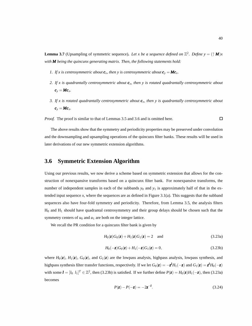
40

Lemma 3.7(Upsampling of symmetric sequence). Let x be a sequence defined onZ2. Define y= (↑ MMM)x

with MMM being the quincunx generating matrix. Then, the followingstatements hold:

1. If x is centrosymmetric about cccx, then y is centrosymmetric about cccy = MMMcccx.

2. If x is quadrantally centrosymmetric about cccx, then y is rotated quadrantally centrosymmetric about

cccy = MMMcccx.

3. If x is rotated quadrantally centrosymmetric about cccx, then y is quadrantally centrosymmetric about

cccy = MMMcccx.

Proof. The proof is similar to that of Lemmas 3.5 and 3.6 and is omitted here.

The above results show that the symmetry and periodicity properties may be preserved under convolution

and the downsampling and upsampling operations of the quincunx filter banks. These results will be used in

later derivations of our new symmetric extension algorithms.

3.6 Symmetric Extension Algorithm

Using our previous results, we now derive a scheme based on symmetric extension that allows for the con-

struction of nonexpansive transforms based on a quincunx filter bank. For nonexpansive transforms, the

number of independent samples in each of the subbandsy0 andy1 is approximately half of that in the ex-

tended input sequencex, where the sequences are as defined in Figure 3.1(a). This suggests that the subband

sequences also have four-fold symmetry and periodicity. Therefore, from Lemma 3.5, the analysis filters

H0 and H1 should have quadrantal centrosymmetry and their group delays should be chosen such that the

symmetry centers ofu0 andu1 are both on the integer lattice.

We recall the PR condition for a quincunx filter bank is given by

H0(zzz)G0(zzz)+H1(zzz)G1(zzz) = 2 and (3.23a)

H0(−zzz)G0(zzz)+H1(−zzz)G1(zzz) = 0, (3.23b)

whereH0(zzz), H1(zzz), G0(zzz), andG1(zzz) are the lowpass analysis, highpass analysis, lowpass synthesis, and

highpass synthesis filter transfer functions, respectively. If we let G0(zzz) = −zzzlll H1(−zzz) andG1(zzz) = zzzlll H0(−zzz)

with somelll = [l0 l1]T ∈ Z2, then (3.23b) is satisfied. If we further defineP(zzz) = H0(zzz)H1(−zzz), then (3.23a)

becomes

P(zzz)−P(−zzz) = −2zzz−lll . (3.24)

41

If H0 and H1 have quadrantal centrosymmetry with group delaysddd0 = [d0,0 d0,1]T andddd1 = [d1,0 d1,1]

T ,

respectively, thenP(zzz) andP(−zzz) are also quadrantally centrosymmetric with group delaydddp = ddd0 +ddd1. We

can see that whenP has more than two nonzero coefficients, in order to satisfy (3.24),P must have even-even

quadrantal centrosymmetry with symmetry centerdddp ∈ Z2\LAT(MMM), and the coefficients ofP are zero at all

non-lattice points exceptdddp.

Now we examine the possible choices of the quadrantally centrosymmetric analysis filters. As previously

shown in Section 3.3, a filter with odd-even, even-odd, or odd-odd quadrantal centrosymmetry cannot be a

good lowpass filter. Therefore, the lowpass analysis filter H0 must have the even-even type of symmetry. In

order forP to have the even-even type of symmetry with group delaydddp ∈ Z2, by using Tables 3.2 and 3.4,

there are altogether four possibilities of the choice of thehighpass analysis filter H1 according to the location

of the group delayddd0 = [d0,0 d0,1]T of the lowpass analysis filter H0:

1. whenddd0 ∈ Z2, H1 must have even-even type symmetry withddd1 ∈ Z2;

2. whend0,0 ∈ 12Zodd andd0,1 ∈Z, H1 must have odd-even type symmetry withd1,0 ∈ 1

2Zodd andd1,1 ∈Z;

3. whend0,0 ∈Z andd0,1 ∈ 12Zodd, H1 must have even-odd type symmetry withd1,0 ∈Z andd1,1 ∈ 1

2Zodd;

4. whenddd0 ∈ 12Z2

odd, H1 must have odd-odd type symmetry withddd1 ∈ 12Z2

odd.

In the remainder of this chapter, we discuss, for each of the above four cases, how one can construct nonex-

pansive transforms with the mapping scheme introduced in Section 3.4.

3.6.1 Type-1 Symmetric Extension Algorithm

We first consider the case where both analysis filters have even-even quadrantal centrosymmetry with group

delaysddd0,ddd1 ∈ Z2. As mentioned earlier, the group delay ofP(zzz) = H0(zzz)H1(−zzz) should satisfy thatdddp =

ddd0 +ddd1 ∈ Z2 \LAT(MMM). Therefore, it follows thatddd0 andddd1 are in different cosets of the quincunx lattice.

This suggests that such a PR filter bank is compatible with thetype-1 symmetric extension scheme in (3.8)

and leads to the result below.

Theorem 3.8(Type-1 symmetric extension algorithm). Consider the filter bank shown in Figure 3.1, where

the input sequencex is defined on the rectangular region{0,1, . . . ,L0−1}×{0,1, . . . ,L1−1} and x is the

type-1 symmetric extension ofx as given by (3.8). If H0 and H1 are quadrantally centrosymmetric with group

delays ddd0 = [d0,0 d0,1]T ∈ Z2 and ddd1 = [d1,0 d1,1]

T ∈ Z2, respectively, and ddd0 and ddd1 are in different

cosets of the quincunx lattice, then the subband output y0 can be completely characterized by N0 samples

42

with indices nnn = [n0 n1]T given by

⌈d0,0+d0,1

2

⌉

≤ n0 ≤⌊

d0,0+d0,1+L0+L1

2

⌋

−1, and

max{d0,0−n0,n0−d0,1−L1 +1} ≤ n1 ≤ min{d0,0+L0−1−n0,n0−d0,1};

(3.25)

y1 can be completely characterized by N1 samples with indices nnn = [n0 n1]T given by

⌈d1,0+d1,1

2

⌉

≤ n0 ≤⌊

d1,0+d1,1+L0+L1

2

⌋

−1, and

max{d1,0−n0,n0−d1,1−L1 +1} ≤ n1 ≤ min{d1,0+L0−1−n0,n0−d1,1};

(3.26)

and N0 +N1 = L0L1, i.e., the transform is nonexpansive.

Proof. In what follows, we refer to the definitions of sequences in Figure 3.1(a). From Lemma 3.1, we know

thatx is PPP-periodic withPPP =[

2L0−2 00 2L1−2

]

, and is quadrantally centrosymmetric about 000. Consider the first

channel, where H0 is quadrantally centrosymmetric with group delayddd0 ∈ Z2. Then, the analysis filter output

u0 is PPP-periodic from Lemma 3.3, and quadrantally centrosymmetric about 000+ddd0 = ddd0 from Lemma 3.2.

SinceMMM−1PPP =[

L0−1 L1−1L0−1 −L1+1

]

is an integer matrix andddd0 ∈ Z2, y0 is MMM−1PPP-periodic from Lemma 3.4, and

rotated quadrantally centrosymmetric aboutMMM−1ddd0 from Lemma 3.5.

Therefore,y0 can be completely characterized by samples with indicesnnn = [n0 n1]T given by

MMMnnn∈ {d0,0,d0,0 +1, . . . ,d0,0 +L0−1}×{d0,1,d0,1 +1, . . . ,d0,1 +L1−1}. (3.27)

Solving (3.27), we obtain the conditions forn0 andn1 as shown in (3.25). The numberN0 of characteristic

samples ofy0 is given by

N0 =

12L0L1 for L0L1 even

12(L0L1 +1) for L0L1 odd,ddd0 ∈ LAT(MMM)

12(L0L1−1) for L0L1 odd,ddd0 6∈ LAT(MMM)

(3.28)

which can be equivalently written as

N0 =⌊1

2(L0L1 +d0,0+d0,1+1)⌋−⌈1

2(d0,0 +d0,1)⌉.

Similarly, y1 is characterized by samples with indicesnnn = [n0 n1]T given by (3.26). The numberN1 of

characteristic samples ofy1 is given by

N1 =

12L0L1 for L0L1 even

12(L0L1 +1) for L0L1 odd,ddd1 ∈ LAT(MMM)

12(L0L1−1) for L0L1 odd,ddd1 6∈ LAT(MMM).

(3.29)

43

Since only one ofddd0 andddd1 is on the quincunx lattice, from (3.28) and (3.29), we haveN0 +N1 = L0L1.

Below, we show an example of the type-1 symmetric extension algorithm. We first give a quincunx filter

bank satisfying the conditions in Theorem 3.8, then apply this filter bank to a finite-extent input sequence.

Example 3.2(Type-1 symmetric extension algorithm). The filter bank is constructed using the method pro-

posed in [6] with two primal and two dual vanishing moments. This filter bank was also proposed in [34].

Using the matrix notation defined in (2.2) in Section 2.3.1, the impulse responses of the analysis filters H0

and H1 are expressed by

h0[nnn] ∼ 132

0 0 −1 0 0

0 −2 4 −2 0

−1 4 28 4 −1

0 −2 4 −2 0

0 0 −1 0 0

and h1[nnn] ∼ 14

0 −1 0

−1 4 -1

0 −1 0

, (3.30)

and the group delays are[0 0]T and[−1 0]T , respectively. The synthesis filter transfer functions arecom-

puted asG0(zzz) = −z−10 H1(−zzz) andG1(zzz) = z−1

0 H0(−zzz). The frequency responses of the filters are shown

in Figure 3.6, and the primal/dual scaling and wavelet functions are depicted in Figure 3.7.

We apply this filter bank to the input sequence ˜x in Example 3.1 as shown in Figure 3.5(a), which contains

four independent samplesa, b, c, andd defined on{0,1}×{0,1}. We use the symmetric extension structure

shown in Figure 3.1(a). The type-1 extended sequencex is shown in Figure 3.5(b). The sequencesu0, u1

andy0, y1 are shown in Figure 3.8. For each sequence, the boldface samples represent points on the lattice

generated by the periodicity matrix of this sequence, the dot represents the symmetry center, and the samples

inside the dashed lines are the independent samples of this sequence. We can see from Figures 3.8(c) and (d)

that the subband sequence ˜y0 has two independent samples14(3a−d+b+c) and 1

4(3d−a+b+c) located

at (0,0) and(1,0), respectively, and ˜y1 has two independent samplesc− 12(a+d) andb− 1

2(a+d) located

at (1,−1) and(1,0), respectively. The above results are consistent with the results in Theorem 3.8.


Recall that at the beginning of Section 3.6, we have introduced four types of quadrantally centrosymmetric

PR quincunx filter banks. In this section, we consider the second type of PR filter bank, where H1 has the odd-

even quadrantal centrosymmetry, and the group delays of H0 and H1 satisfyd0,0,d1,0 ∈ 12Zodd, d0,1,d1,1 ∈ Z,

andddd0 +ddd1 ∈ Z2 \LAT(MMM). In order for this filter bank to have the nonexpansive property, the sequences

44

−1

−0.5

0

0.5

−1

−0.5

0

0.5

0

0.2

0.4

0.6

0.8

1

Fx

Fy

Mag

nitu

de

−1

−0.5

0

0.5

−1

−0.5

0

0.5

0

0.5

1

1.5

2

Fx

Fy

Mag

nitu

de

(a) (b)

−1

−0.5

0

0.5

−1

−0.5

0

0.5

0

0.5

1

1.5

2

Fx

Fy

Mag

nitu

de

−1

−0.5

0

0.5

−1

−0.5

0

0.5

0

0.2

0.4

0.6

0.8

1

Fx

Fy

Mag

nitu

de

c) (d)

Figure 3.6: Frequency responses of the (a) lowpass analysis, (b) highpass analysis, (c) lowpass synthesis, and

(d) highpass synthesis filters for a type-1 filter bank.

(a) (b) (c) (d)

Figure 3.7: Scaling and wavelet functions for a type-1 filterbank. The (a) primal wavelet, (b) primal scaling,

(c) dual wavelet, and (d) dual scaling functions.

45

1

4(3d − a+b + c)

1

4(3c − b+a + d)

1

4(3d − a+b + c)

1

4(3c − b+a + d)

1

4(3b − c+a + d)

1

4(3a − d1

4(3a − d1

4(3a − d+b + c)+b + c)+b + c)

1

4(3b − c+a + d)

1

4(3a − d1

4(3a − d1

4(3a − d+b + c)+b + c)+b + c)

1

4(3d − a+b + c)

1

4(3c − b+a + d)

1

4(3d − a+b + c)

1

4(3c − b+a + d)

1

4(3b − c+a + d)

1

4(3a − d1

4(3a − d1

4(3a − d+b + c)+b + c)+b + c)

1

4(3b − c+a + d)

1

4(3a − d1

4(3a − d1

4(3a − d+b + c)+b + c)+b + c)

b − a + d

2a − b + c

2b − a + d

2a − b + c

2

d − b + c

2c − a + d

2c − a + d

2c − a + d

2d − b + c

2c − a + d

2c − a + d

2c − a + d

2

b − a + d

2a − b + c

2b − a + d

2a − b + c

2

d − b + c

2c − a + d

2c − a + d

2c − a + d

2d − b + c

2c − a + d

2c − a + d

2c − a + d

2

(a) (b)

1

4(3a − d1

4(3a − d1

4(3a − d+b + c)+b + c)+b + c)

1

4(3d − a+b + c)

1

4(3a − d1

4(3a − d1

4(3a − d+b + c)+b + c)+b + c)

1

4(3d − a+b + c)

1

4(3d − a+b + c)

1

4(3a − d1

4(3a − d1

4(3a − d+b + c)+b + c)+b + c)

1

4(3d − a+b + c)

1

4(3a − d1

4(3a − d1

4(3a − d+b + c)+b + c)+b + c)

1

4(3a − d1

4(3a − d1

4(3a − d+b + c)+b + c)+b + c)

1

4(3d − a+b + c)

1

4(3a − d1

4(3a − d1

4(3a − d+b + c)+b + c)+b + c)

1

4(3d − a+b + c)

1

4(3d − a+b + c)

1

4(3a − d1

4(3a − d1

4(3a − d+b + c)+b + c)+b + c)

1

4(3d − a+b + c)

1

4(3a − d1

4(3a − d1

4(3a − d+b + c)+b + c)+b + c)

c − a + d

2c − a + d

2c − a + d

2b − a + d

2c − a + d

2c − a + d

2c − a + d

2b − a + d

2

b − a + d

2c − a + d

2c − a + d

2c − a + d

2b − a + d

2c − a + d

2c − a + d

2c − a + d

2

c − a + d

2c − a + d

2c − a + d

2b − a + d

2c − a + d

2c − a + d

2c − a + d

2b − a + d

2

b − a + d

2c − a + d

2c − a + d

2c − a + d

2b − a + d

2c − a + d

2c − a + d

2c − a + d

2

(c) (d)

Figure 3.8: The intermediate sequences (a)u0, (b) u1 and output sequences (c)y0, (d) y1 in the type-1 filter

bank. The sequences are as defined in Figure 3.1(a).

46

y0 andy1, as defined in Figure 3.1(a), should have four-fold symmetryand periodicity. This requires the

sequencesu0 andu1 to be quadrantally centrosymmetric with symmetry centers on the integer latticeZ2.

These observations suggest that this type of PR filter bank may be compatible with the type-2 symmetric

extension defined in (3.8), where the extended sequencex is half-sample symmetric in the horizontal direction

and whole-sample symmetric in the vertical direction. This, in fact, is the case, as demonstrated by the

theorem below.

Theorem 3.9 (Type-2 symmetric extension algorithm). Consider the analysis filter bank shown in Fig-

ure 3.1(a), where the input sequencex is defined on the rectangular region{0,1, . . . ,L0−1}×{0,1, . . . ,L1−1} and x is the type-2 symmetric extension ofx as given by (3.8). Let MMM denote the quincunx generat-

ing matrix[

1 11 −1

]. Suppose that the analysis filters H0 and H1 satisfy the following conditions: 1) H0 has

even-even quadrantal centrosymmetry with group delay ddd0 = [d0,0 d0,1]T , d0,0 ∈ 1

2Zodd and d0,1 ∈ Z; 2) H1

has odd-even quadrantal centrosymmetry with group delay ddd1 = [d1,0 d1,1]T , d1,0 ∈ 1

2Zodd and d1,1 ∈ Z;

3) ddd0−ddd1 ∈ LAT(MMM). In this case, the subband output y0 can be completely characterized by N0 samples

with indices nnn = [n0 n1]T given by⌈

d0,0+d0,1− 12

2

⌉

≤ n0 ≤⌊

d0,0+d0,1+L0 +L1− 32

2

⌋

and

max{d0,0−n0− 12,n0−d0,1−L1+1} ≤ n1 ≤ min{d0,0+L0−n0− 1

2,n0−d0,1};

(3.31)


⌈

d1,0+d1,1+ 12

2

⌉

≤ n0 ≤⌊

d1,0+d1,1+L0 +L1− 52

2

⌋

and

max{d1,0−n0+ 12,n0−d1,1−L1+1} ≤ n1 ≤ min{d1,0+L0−n0− 3

2,n0−d1,1};

(3.32)


Proof. In what follows, we refer to the definitions of sequences in Figure 3.1(a). From Lemma 3.1, we

know thatx is PPP-periodic withPPP =[

2L0 00 2L1−2

]

and quadrantally centrosymmetric about[

−12 0]T

. Consider

the first channel, where H0 is quadrantally centrosymmetric with group delayddd0 = [d0,0 d0,1]T satisfying

d0,0 ∈ 12Zodd and d0,1 ∈ Z. Then, the analysis filter outputu0 is PPP-periodic from Lemma 3.3 and quad-

rantally centrosymmetric aboutcccu0 =[d0,0− 1

2 d0,1]T

from Lemma 3.2. SinceMMM−1PPP =[

L0 L1−1L0 −L1+1

]

is an

integer matrix andcccu0 ∈ Z2, y0 is MMM−1PPP-periodic from Lemma 3.4 and rotated quadrantally centrosymmet-

ric aboutMMM−1cccu0 from Lemma 3.5. Therefore,y0 can be completely characterized by samples with indices

nnn = [n0 n1]T given by

MMMnnn∈ {d0,0− 12,d0,0 + 1

2, . . . ,d0,0 +L0− 12}×{d0,1,d0,1 +1, . . . ,d0,1+L1−1}. (3.33)

47

Solving (3.33), we obtain the conditions forn0 andn1 as shown in (3.31). The numberN0 of characteristic


N0=

12(L0 +1)L1 for (L0 +1)L1 even

12

[(L0 +1)L1 +1

]for (L0 +1)L1 odd,cccu0 ∈ LAT(MMM)

12

[(L0 +1)L1−1

]for (L0 +1)L1 odd,cccu0 6∈ LAT(MMM).

(3.34)

The above equation can be equivalently written as

N0 =⌊ 1

2((L0+1)L1+d0,0+d0,1+12)⌋−⌈1

2(d0,0+d0,1− 12)⌉.

Now we consider the second channel. Similar to the case of thefirst channel, we know thatu1 is PPP-

periodic and quadrantally centrosymmetric aboutcccu1 =[d1,0− 1

2 d1,1]T

. Since H1 has odd-even symmetry,

u1 also has odd-even symmetry. Note that each 1D horizontal slice of u1 has whole-sample antisymmetry.

Then,y1 can be completely characterized by samples with indicesnnn = [n0 n1]T given by

MMMnnn∈ {d1,0+ 12,d1,0 + 3

2, . . . ,d1,0 +L0− 32}×{d1,1,d1,1 +1, . . . ,d1,1+L1−1}. (3.35)

Solving (3.35), we obtain the conditions forn0 andn1 as shown in (3.32). The number of characteristic


N1=

12(L0−1)L1 for (L0−1)L1 even

12

[(L0−1)L1−1

]for (L0−1)L1 odd,cccu1 ∈ LAT(MMM)

12

[(L0−1)L1 +1

]for (L0−1)L1 odd,cccu1 6∈ LAT(MMM).

(3.36)

The above equation can be simplified as

N1 =⌊

12((L0−1)L1+d1,0+d1,1+

32)⌋−⌈

12(d1,0+d1,1+

12)⌉.

Sinceddd0−ddd1 ∈ LAT(MMM), cccu0 andcccu1 are in the same coset of the quincunx lattice. Therefore, from (3.34)

and (3.36), we haveN0 +N1 = L0L1.

The above theorem is illustrated by the following example. Aquincunx filter bank satisfying the three

conditions in Theorem 3.9 is given, then it is applied to the input sequence in Example 3.1.

Example 3.3 (Type-2 symmetric extension algorithm). An example of this type of PR filter bank is the

Haar-like filter bank given by the transfer functions

H0(z0,z1) = 12 (1+z0) ,H1(z0,z1) = 1−z0,G0(z0,z1) = 1+z−1

0 , andG1(z0,z1) = 12

(−1+z−1

0

).

48

−1

−0.5

0

0.5

−1

−0.5

0

0.5

0

0.2

0.4

0.6

0.8

1

Fx

Fy

Mag

nitu

de

−1

−0.5

0

0.5

−1

−0.5

0

0.5

0

0.5

1

1.5

2

Fx

Fy

Mag

nitu

de

(a) (b)

−1

−0.5

0

0.5

−1

−0.5

0

0.5

0

0.5

1

1.5

2

Fx

Fy

Mag

nitu

de

−1

−0.5

0

0.5

−1

−0.5

0

0.5

0

0.2

0.4

0.6

0.8

1

Fx

Fy

Mag

nitu

de

c) (d)


(d) highpass synthesis filters for the Haar-like filter bank.

(a) (b) (c) (d)

Figure 3.10: Scaling and wavelet functions for the Haar-like filter bank. The (a) primal wavelet, (b) primal

scaling, (c) dual wavelet, and (d) dual scaling functions.

49

c + d

2c

c + d

2d

c + d

2c

c + d

2

a + b

2a a + b

2

a + b

2

a + b

2b

a + b

2a

a + b

2

a + b

2

a + b

2

c + d

2c

c + d

2d

c + d

2c

c + d

2

a + b

2a

a + b

2

a + b

2

a + b

2b

a + b

2a

a + b

2

a + b

2

a + b

2

d − c 0 c − d 0 d − c 0 c − d

b − a0

a − ba − ba − b 0 b − a 0 a − ba − ba − b

d − c 0 c − d 0 d − c 0 c − d

b − a 0 a − ba − ba − b 0 b − a 0 a − ba − ba − b

(a) (b)

da + b

2c

a + b

2

a + b

2

a + b

2d

a + b

2c

a + b

2c

a + b

2

a + b

2

a + b

2d

a + b

2c

a + b

2

a + b

2

a + b

2

ca + b

2

a + b

2

a + b

2d

a + b

2c

a + b

2

a + b

2

a + b

2d

a + b

2

a + b

2

a + b

2d

a + b

2c

a + b

2

a + b

2

a + b

2d

a + b

2

0 b − a 0 a − ba − ba − b 0 b − a 0

b − a 0 a − ba − ba − b 0 b − a 0 a − ba − ba − b

0 a − ba − ba − b 0 b − a 0 a − ba − ba − b 0

a − ba − ba − b 0 b − a 0 a − ba − ba − b 0 b − a

(c) (d)

Figure 3.11: The intermediate sequences (a)u0, (b) u1 and output sequences (c)y0, (d) y1 in the Haar-like

filter bank. The sequences are as defined in Figure 3.1(a).

The group delays of the analysis filters are both[− 12 0]T . The frequency responses are shown in Figure 3.9,

and the scaling and wavelet functions associated with this filter bank are illustrated in Figure 3.10.

We apply this filter bank to Example 3.1 given in Section 3.4 with the type-2 symmetric extension, where

the original input sequence ˜x with four samples is shown in Figure 3.5(a), and the extendedsequencex is

shown in Figure 3.5(c). The outputsu0, u1, y0, andy1, as defined in Figure 3.1(a), are shown in Figure 3.11,

where the boldface samples represent points on the periodicity lattice, the dot represents the symmetry center,

and the independent samples of each sequence are located inside the area surrounded by the dashed lines.

From Figures 3.11(c) and (d), we see that ˜y0 has three independent samples12(a+ b), c and d at (0,0),

(0,−1) and(1,0), respectively, and ˜y1 has only one independent samplea−b at (0,0). The total number of

independent samples in the subbands is four. Thus, the transform is nonexpansive.

50


Recall that there are four types of PR quincunx filter banks with quadrantally centrosymmetric filters. Next

we consider the third type, where H1 is even-odd quadrantally centrosymmetric. In the below theorem, we

show this type of filter bank is compatible with the type-3 symmetric extension defined in (3.8), where the

extended sequencex has whole-sample symmetry in the horizontal direction and half-sample symmetry in

the vertical direction.

Theorem 3.10(Type-3 symmetric extension algorithm). Consider the analysis filter bank shown in Fig-

ure 3.1(a), wherex is defined on the rectangular region{0,1, . . . ,L0 − 1}× {0,1, . . . ,L1 −1} and x is the

type-3 symmetric extension ofx as given by (3.8). Let MMM denote the quincunx generating matrix[

1 11 −1

].

Suppose that the analysis filters H0 and H1 satisfy the following conditions: 1) H0 has even-even quadrantal

centrosymmetry with group delay ddd0 = [d0,0 d0,1]T , d0,0 ∈ Z and d0,1 ∈ 1

2Zodd; 2) H1 has even-odd quad-

rantal centrosymmetry with group delay ddd1 = [d1,0 d1,1]T , d1,0 ∈Z and d1,1 ∈ 1

2Zodd; 3) ddd0−ddd1 ∈ LAT(MMM).

In this case, the subband output y0 can be completely characterized by N0 samples with indices nnn= [n0 n1]T

given by⌈

d0,0 +d0,1− 12

2

⌉

≤ n0 ≤⌊

d0,0+d0,1+L0+L1− 32

2

⌋

and

max{d0,0−n0,n0−d0,1−L1 + 12} ≤ n1 ≤ min{d0,0+L0−n0−1,n0−d0,1+ 1

2};

(3.37)

y1 can be completely characterized by N1 samples given by⌈

d1,0 +d1,1+ 12

2

⌉

≤ n0 ≤⌊

d1,0+d1,1+L0+L1− 52

2

⌋

and

max{d1,0−n0,n0−d1,1−L1 + 32} ≤ n1 ≤ min{d1,0+L0−n0−1,n0−d1,1− 1

2};

(3.38)


This theorem can be proved in a way similar to that of Theorem 3.9 with interchanged horizontal and

vertical indices. An example of this type of PR filter bank is given by the analysis and synthesis filter transfer

functions

H0(z0,z1) = 12 (1+z1) ,H1(z0,z1) = 1−z1,G0(z0,z1) = 1+z−1

1 , andG1(z0,z1) = 12

(z−11 −1

).

3.6.4 Type-4 PR Quincunx Filter Banks

We have discussed three out of the four types of quadrantallycentrosymmetric PR quincunx filter banks in

the preceding sections. Now we show that for the last type of PR quincunx filter bank, where H1 is odd-odd

51

quadrantally centrosymmetric with group delayddd1 ∈ 12Z2

odd, no nonexpansive transform can be constructed

for any of the symmetric extension schemes defined in (3.8). In this case, the total number of independent

samples in the subband sequencesy0 andy1 combined is always greater than that in the original finite-extent

sequence ˜x. We prove this statement in a constructive way. In what follows, we refer to the definitions of

sequences in Figure 3.1(a).

For this type of PR quincunx filter bank, the analysis filters H0 and H1 have even-even and odd-odd

quadrantal centrosymmetry, respectively, and their groupdelays satisfy thatddd0,ddd1 ∈ 12Z2

odd. In order for the

filter bank to be nonexpansive, the subband sequencesy0 andy1 are required to have four-fold symmetry

and periodicity. It follows that the symmetry center of the extended sequencex satisfiescccx ∈ 12Z2

odd. From

Lemma 3.1, we know the original input ˜x should be extended using the type-4 symmetric extension defined

in (3.8). Then,x is quadrantally centrosymmetric aboutcccx = [− 12 − 1

2 ]T , and[

2L0 00 2L1

]

-periodic. In this

case, the subband sequencey0 has rotated quadrantal centrosymmetry with symmetry center cccy0 ∈ Z2 and

periodicity withMMM−1PPP =[

L0 L1L0 −L1

]

. Therefore,y0 can be completely characterized by samples with indices

nnn = [n0 n1]T given by

MMMnnn∈ {d0,0− 12,d0,0 + 1

2, . . . ,d0,0 +L0− 12}×{d0,1− 1

2,d0,1 + 12, . . . ,d0,1 +L1− 1

2},

and the number of independent samples iny0 is

N0 =

12(L0 +1)(L1 +1) for (L0 +1)(L1 +1) even

12

[(L0 +1)(L1+1)+1

]for (L0 +1)(L1 +1) odd,(ddd0 +cccx) ∈ LAT(MMM)

12

[(L0 +1)(L1+1)−1

]for (L0 +1)(L1 +1) odd,(ddd0 +cccx) 6∈ LAT(MMM).

Similarly, for the second channel, sinceu1 has odd-odd type quadrantal centrosymmetry,y1 can be completely

characterized byN1 samples with indicesnnn = [n0 n1]T given by

MMMnnn∈ {d1,0+ 12,d1,0 + 3

2, . . . ,d1,0 +L0− 32}×{d1,1+ 1

2,d1,1 + 32, . . . ,d1,1 +L1− 3

2}, and

N1 =

12(L0−1)(L1−1) for (L0−1)(L1−1) even

12

[(L0−1)(L1−1)+1

]for (L0−1)(L1−1) odd,(ddd1 +cccx) ∈ LAT(MMM)

12

[(L0−1)(L1−1)−1

]for (L0−1)(L1−1) odd,(ddd1 +cccx) 6∈ LAT(MMM).

We can see that when(L0+1)(L1+1)∈Zeven, the total number of independent samples iny0 andy1 is always

L0L1 +1. Therefore, we cannot construct nonexpansive transformsusing this type of PR filter bank.

52

3.6.5 Octave-Band Decomposition

A weakness of the symmetric extension algorithms introduced in the preceding sections is that they cannot

be used in an octave-band decomposition where the filter bankis applied recursively in the lowpass channel.

With the proposed algorithms in Theorems 3.8, 3.9, and 3.10,the extent of the lowpass output sequence

y0 assumes the shape of a 45◦-rotated rectangle. At the second level of an octave-band decomposition, ˜y0

becomes the input sequence to the symmetric extension structure in Figure 3.1(a), while this structure only

operates on sequences defined in rectangular regions. Therefore, these algorithms cannot be applied to an

octave-band filter bank. For the type-1 symmetric extensionalgorithm, however, if we constrain the analysis

filters more tightly, the filter bank can still be used to construct nonexpansive transforms with an octave-band

decomposition, as demonstrated by the below theorem.

Theorem 3.11(Type-1 symmetric extension algorithm for octave-band decompositions). Consider the two-

level octave-band filter bank shown in Figure 3.12, wherex is defined on the rectangular region{0,1, . . . ,L0−1}× {0,1, . . . ,L1 − 1} and x is the type-1 symmetric extension ofx as given by (3.8). If H0 and H1 have

both quadrantal and rotated-quadrantal centrosymmetry, and their group delays ddd0 and ddd1 satisfy that ddd0 =

[d0,0 d0,1]T ∈ LAT(MMM) and ddd1 = [d1,0 d1,1]

T ∈ Z2 \ LAT(MMM), respectively, then the subband output y00

can be completely characterized by N00 samples with indices nnn = [n0 n1]T given by

d0,0 +

⌈d0,1

2

⌉

≤ n0 ≤ d0,0 +

⌊d0,1

2

⌋

+

⌊L0−1

2

⌋

and

⌈d0,0

2

⌉

≤ n1 ≤⌊

d0,0

2

⌋

+

⌊L1−1

2

⌋

; (3.39)


⌈d0,0 +d1,0+d1,1

2

⌉

≤ n0 ≤⌊

d0,0 +d1,0+d1,1

2

⌋

+

⌊L0−1

2

⌋

, and

⌈d0,1 +d1,0−d1,1

2

⌉

≤ n1 ≤⌊

d0,1+d1,0−d1,1

2

⌋

+

⌊L1−1

2

⌋

;

(3.40)

y1 can be completely characterized by N1 samples with indices nnn = [n0 n1]T given by (3.26); and N00+

N01+N1 = L0L1, i.e., the transform is nonexpansive.

Proof. From Theorem 3.8, we know thaty0 has rotated quadrantal centrosymmetry aboutcccy0 = MMM−1ddd0 ∈ Z2

andPPPy0-periodicity withPPPy0 = MMM−1PPP=[

L0−1 L1−1L0−1 −L1+1

]

∈ LAT(MMM), and its independent samples are located in

a finite region given by (3.25).

At the second decomposition level, since H0 has rotated quadrantal centrosymmetry, from Lemma 3.2,

u00 is also rotated quadrantally centrosymmetric with symmetry centercccu00 = cccy0 +ddd0 ∈ Z2 and periodic

with periodicity matrixPPPy0 ∈ LAT(MMM). From Lemmas 3.4 and 3.5,y00 has quadrantal centrosymmetry with

53

H0(zzz)

H1(zzz)

↓ MMM

↓ MMM

H0(zzz)

H1(zzz)

↓ MMM

↓ MMM





x[nnn] x[nnn] u0[nnn]

u1[nnn]

y0[nnn] u00[nnn]

u01[nnn]

y00[nnn]

y01[nnn]

y1[nnn]

y00[nnn]

y01[nnn]

y1[nnn]

Figure 3.12: Symmetric extension for two-level octave-band filter banks.

symmetry centercccy00 andPPPy00-periodicity, where

cccy00 = MMM−1cccu00 = MMM−2ddd0 +ddd0 =[d0,0+ 1

2d0,112d0,0

]Tand (3.41)

PPPy00 = MMM−2PPP =[

L0−1 00 L1−1

]

.

Therefore,y00 can be completely characterized by samples with indicesnnn given by

⌈cccy00

⌉≤ nnn≤

⌊cccy00

⌋+⌊

12 [L0−1 L1−1]T

⌋

. (3.42)

Substituting (3.41) into (3.42), we obtain the indices of the independent samples iny00 as in (3.39). The

number of the independent samples is calculated as

N00 =

⌊L0+1

2

⌋⌊L1+1

2

⌋

for ddd0 ∈ Z2even

⌈L0−1

2

⌉⌈L1−1

2

⌉

for ddd0 ∈ Z2odd.

(3.43)

Next we consider the channel with subband sequencey01. Similarly, y01 has quadrantal centrosymmetry

with symmetry centercccy01 andPPPy01-periodicity, where

cccy01 =[

12(d0,0 +d1,0+d1,1)

12(d0,1+d1,0−d1,1)

]TandPPPy01 = MMM−2PPP =

[L0−1 0

0 L1−1

]

.

Sinceddd1 ∈ Z2 \ LAT(MMM), we haved1,0 + d1,1 ∈ Zodd. Therefore,y01 can be completely characterized by

samples with indicesnnn given by

⌈cccy01

⌉≤ nnn≤

⌊cccy01

⌋+⌊

12 [L0−1 L1−1]T

⌋

.

The preceding inequality can be rewritten as (3.40). Sinceddd1 ∈ Z2\LAT(MMM), d1,0+d1,1 ∈ Zodd, the number

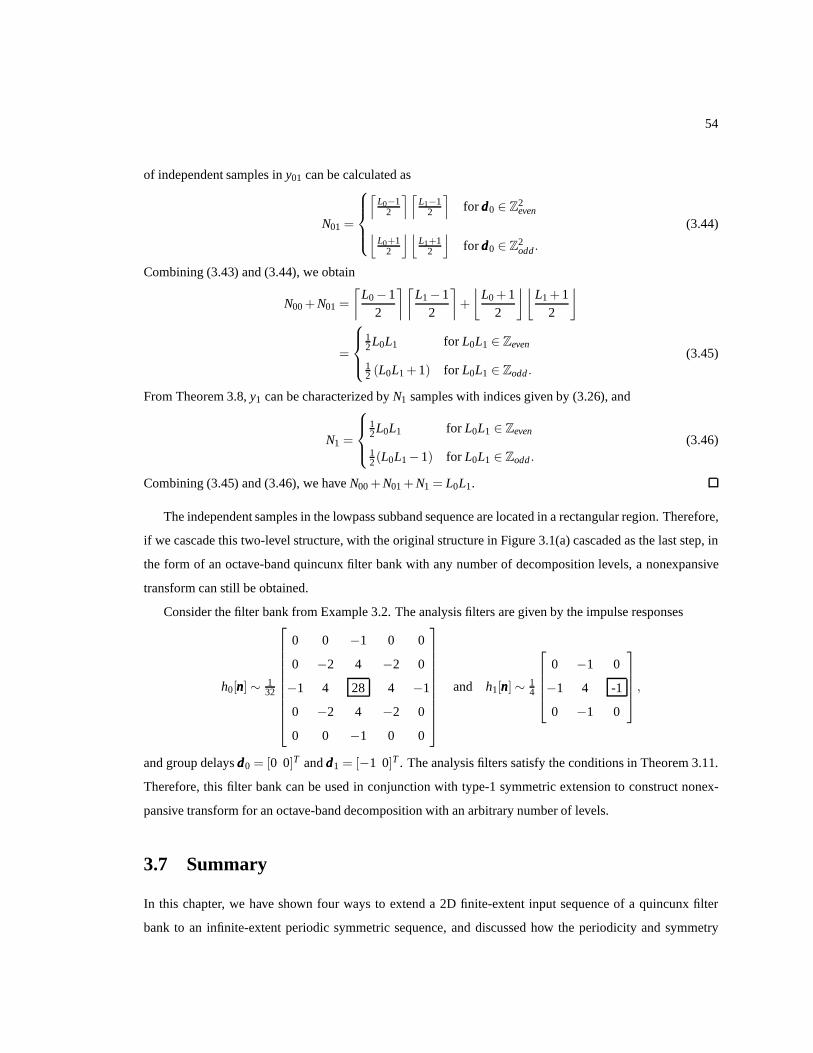
54

of independent samples iny01 can be calculated as

N01 =

⌈L0−1

2

⌉⌈L1−1

2

⌉

for ddd0 ∈ Z2even

⌊L0+1

2

⌋⌊L1+1

2

⌋

for ddd0 ∈ Z2odd.

(3.44)

Combining (3.43) and (3.44), we obtain

N00+N01 =

⌈L0−1

2

⌉⌈L1−1

2

⌉

+

⌊L0 +1

2

⌋⌊L1 +1

2

⌋

=

12L0L1 for L0L1 ∈ Zeven

12 (L0L1 +1) for L0L1 ∈ Zodd.

(3.45)

From Theorem 3.8,y1 can be characterized byN1 samples with indices given by (3.26), and

N1 =

12L0L1 for L0L1 ∈ Zeven

12(L0L1−1) for L0L1 ∈ Zodd.

(3.46)

Combining (3.45) and (3.46), we haveN00+N01+N1 = L0L1.

The independent samples in the lowpass subband sequence arelocated in a rectangular region. Therefore,

if we cascade this two-level structure, with the original structure in Figure 3.1(a) cascaded as the last step, in

the form of an octave-band quincunx filter bank with any number of decomposition levels, a nonexpansive

transform can still be obtained.

Consider the filter bank from Example 3.2. The analysis filters are given by the impulse responses

h0[nnn] ∼ 132

0 0 −1 0 0

0 −2 4 −2 0

−1 4 28 4 −1

0 −2 4 −2 0

0 0 −1 0 0

and h1[nnn] ∼ 14

0 −1 0

−1 4 -1

0 −1 0

,

and group delaysddd0 = [0 0]T andddd1 = [−1 0]T . The analysis filters satisfy the conditions in Theorem 3.11.

Therefore, this filter bank can be used in conjunction with type-1 symmetric extension to construct nonex-

pansive transform for an octave-band decomposition with anarbitrary number of levels.

3.7 Summary

In this chapter, we have shown four ways to extend a 2D finite-extent input sequence of a quincunx filter

bank to an infinite-extent periodic symmetric sequence, anddiscussed how the periodicity and symmetry

55

properties of the extended sequence can be preserved by the operations of the quincunx filter banks. Then,

we have proposed new algorithms to construct nonexpansive transforms for three types of quadrantally cen-

trosymmetric PR quincunx filter banks. At last, we have shownhow the type-1 algorithm can be extended for

use with multi-level octave-band decompositions. These symmetric extension schemes are potentially useful

in applications that process finite-extent sequences usingquincunx filter banks.

56

Chapter 4

Optimal Design of Quincunx Filter

Banks

4.1 Overview

In this chapter, new optimization-based techniques are proposed for the design of high-performance quincunx

filter banks for the application of image coding. These new methods are used to build linear-phase PR systems

with high coding gain, good analysis/synthesis filter frequency responses, and certain prescribed vanishing

moment properties. Examples of filter banks designed using these techniques are presented and shown to be

highly effective for image coding. The material in this chapter has also been partly presented in [39].

4.2 Introduction

Filter banks have proven to be a highly effective tool for image coding applications [40]. Compared to the

case with 1D filter banks, the nonseparable 2D filter banks aremuch more difficult to design and far fewer

effective methods have been proposed. In image coding applications, one typically desires filter banks to have

PR, linear phase, high coding gain, good frequency selectivity, and satisfactory vanishing moment properties.

The PR property is desirable as it facilitates the construction of a lossless compression system. That is,

if the system possesses this property, then in absence of quantization, the original image can be precisely

reproduced from the subband coefficients. The linear phase property is crucial to avoiding phase distortion.

High coding gain often leads to efficient energy compaction of images. The presence of vanishing moments

57

helps reduce the number of nonzero coefficients in the highpass subbands, and good frequency selectivity can

diminish aliasing in the subband signals. Designing nonseparable 2D filter banks with all of the preceding

properties is an extremely challenging task. In this chapter, several new optimization-based techniques are

proposed for constructing quincunx filter banks with all of the aforementioned desirable characteristics.

The remainder of this chapter is organized as follows. Section 4.3 presents a parametrization of linear-

phase PR quincunx filter banks based on the lifting scheme. Wechoose the lifting-based parametrization

because the PR and linear-phase properties can be structurally imposed on the filter bank, which simplifies

the later optimization algorithms. Then, an optimal designalgorithm for quincunx filter banks with two

lifting steps is proposed in Section 4.4. In this section, weshow how coding gain, vanishing moments,

and frequency selectivity are related to the lifting-filtercoefficients, and discuss how the design of quincunx

filter banks with all of the desired characteristics can be formulated as a constrained optimization problem.

In Section 4.5, a scheme is proposed for the design of filter banks with more than two lifting steps. In

this case, the relationships between the desirable properties and the lifting filter coefficients become more

complicated than in the two-lifting-step case. We explain how the design can be formulated as a similar

optimization problem. In Section 4.6, a suboptimal design algorithm is proposed for filter banks with at least

three lifting steps using the above two algorithms. Severaldesign examples are presented in Section 4.7

and their effectiveness for image coding is demonstrated inSection 4.8. Finally, the results obtained in this

chapter are summarized in Section 4.9.

4.3 Lifting Parametrization of Linear-Phase PR Quincunx Filter Banks

For filter banks in image processing applications, the PR andlinear phase properties are often highly desir-

able. In this section, we introduce a parametrization of a subset of linear-phase PR quincunx filter banks

based on the lifting scheme. The use of the lifting-based parametrization is helpful in several respects. First,

as discussed in Section 2.3.6, the PR condition is automatically satisfied by such a parametrization. Further-

more, the linear-phase condition can be imposed with relative ease. This eliminates the need for additional

cumbersome constraints for PR and linear phase during optimization. Lastly, reversible integer-to-integer

mappings can be readily constructed from the lifting realization [33]. Recall that with the lifting structure,

the synthesis filters are completely determined by the analysis filters. Therefore, in what follows, we only

consider the analysis side of the filter bank.

The canonical form of the analysis side of a quincunx filter bank with analysis filters H0 and H1 is shown

in Figure 4.1. The lifting realization of the analysis side with 2λ lifting filters {Ak} is shown in Figure 4.2.

58

H0(zzz)

H1(zzz)

↓ MMM

↓ MMM

x[nnn]y0[nnn]

y1[nnn]

Figure 4.1: Analysis side of a quincunx filter bank.

A1(zzz) A2(zzz) A2λ−1(zzz) A2λ(zzz)z0

↓ MMM

↓ MMM +

+

+

+

· · ·

· · ·

· · ·x[nnn]

y0[nnn]

y1[nnn]

Figure 4.2: Analysis side of the lifting realization of a quincunx filter bank.

Without loss of generality, we assume none of the transfer functions{Ak(zzz)} are identically zero, except

possiblyA1(zzz) andA2λ (zzz). Using this lifting structure, the linear-phase conditioncan be satisfied with a

prudent choice of lifting filters{Ak}. In particular, in what follows, we will introduce three lifting-based

parameterizations of PR quincunx filter banks that result inlinear-phase analysis/synthesis filters. The filter

banks associated with these parameterizations are henceforth referred to as type-1, type-2, and type-3 filter

banks.

4.3.1 Type-1 Filter Banks

The first lifting parameterization results in symmetric analysis filters H0 and H1 with group delays on the

integer latticeZ2. The detail regarding the choice of the lifting filters{Ak} in Figure 4.2 is given by the

theorem below.

Theorem 4.1(Construction of type-1 filter banks). Consider a quincunx filter bank constructed from the

lifting scheme with2λ lifting filters as shown in Figure 4.2, where none of the transfer functions{Ak(zzz)} are

identically zero, except possibly A1(zzz) and A2λ (zzz). If the lifting filters{Ak} are symmetric, and the filter Ak

has group delay ccck satisfying

ccck = (−1)k[ 12

12

]T,

then the analysis filters H0 and H1 are symmetric with group delays[0 0]T and[−1 0]T , respectively.

59

Proof. Let the analysis filters associated with the firstk lifting steps be denoted as{

H(k)i

}

for i = 0,1. We

prove this theorem by induction onλ . Considerλ = 0. In this case,H(0)0 (zzz) = 1 andH(0)

1 (zzz) = z0. Thus, the

analysis filters H(0)0 and H(0)

1 have symmetric linear phase with group delays[0 0]T and[−1 0]T , respectively.

Therefore, the theorem holds forλ = 0.

Now, assume that the theorem holds forλ = k (i.e., H(2k)0 and H(2k)

1 have symmetric linear phase with

group delays[0 0]T and[−1 0]T , respectively). Forλ = k+1, from (2.28), we have

H(2k+2)

0,0 (zzz) H(2k+2)0,1 (zzz)

H(2k+2)1,0 (zzz) H(2k+2)

1,1 (zzz)

=

1 A2k+2(zzz)

0 1

1 0

A2k+1(zzz) 1

H(2k)

0,0 (zzz) H(2k)0,1 (zzz)

H(2k)1,0 (zzz) H(2k)

1,1 (zzz)

.

Using the above equation, the analysis filter transfer functions{

H(2k+2)i (zzz)

}

can be computed as

H(2k+2)1 (zzz) = H(2k+1)

1 (zzz) = H(2k)1 (zzz)+A2k+1(zzz

MMM)H(2k)0 (zzz) and (4.1)

H(2k+2)0 (zzz) = H(2k+1)

0 (zzz)+A2k+2(zzzMMM)H(2k+1)


MMM)H(2k+1)1 (zzz). (4.2)

In (4.1), since the lifting filter A2k+1 has symmetric linear phase with group delayccc2k+1 =[−1

2 −12

]T, from

Lemma 3.7,A2k+1(zzzMMM) has symmetric linear phase with group delayMMMccc2k+1 = [−1 0]T . By assumption,

H(2k)0 (zzz) is symmetric with group delay[0 0]T . Then, from Lemma 3.2,A2k+1(zzzMMM)H(2k)

0 (zzz) has symmetric

linear phase with group delay[0 0]T + [−1 0]T = [−1 0]T . Therefore, H(2k+2)1 has linear phase with

group delay[−1 0]T . Similarly, in (4.2),A2k+2(zzzMMM) has symmetric linear phase with group delayMMMccc2k+2 =

[1 0]T . Thus, it follows that H(2k+2)0 has linear phase with group delay[0 0]T . Therefore, the theorem

holds forλ = k+1. This completes the proof.

We henceforth refer to the filter banks constructed using Theorem 4.1 astype-1 filter banks. Below we

show an example of a type-1 filter bank. This filter bank is proposed in [6, 34] and previously discussed in

Example 3.2 in Section 3.6.1.

Example 4.1(Type-1 filter bank). Consider the filter bank from Example 3.2 with the analysis filter impulse

responses

h0[nnn] ∼ 132

0 0 −1 0 0

0 −2 4 −2 0

−1 4 28 4 −1

0 −2 4 −2 0

0 0 −1 0 0

and h1[nnn] ∼ 14

0 −1 0

−1 4 -1

0 −1 0

.

60

This filter bank can be realized using two lifting steps. The impulse responses of the lifting filters A1 and A2

are given by

a1[nnn] ∼−14

1 1

1 1

and a2[nnn] ∼ 18

1 1

1 1

,

and the group delays of A1 and A2 areccc1 =[−1

2 −12

]Tandccc2 =

[12

12

]T, respectively.

In order to allow the frequency responses of the lifting and analysis filters to be expressed in a compact

form, we introduce some notation in this regard. Since the lifting filter Ak has linear phase with group

delayccck = (−1)k [ 12

12 ]T , the support region of Ak is a rectangle of size 2lk,0×2lk,1 for somelk,0, lk,1 ∈ Z+,

and the number of independent coefficients in Ak is 2lk,0lk,1. Let aaak be a vector containing the independent

coefficients of Ak. Then, there are 2lk,0lk,1 elements inaaak indexed from 0 to 2lk,0lk,1−1.

For an odd-indexed lifting filter A2k−1, its support region can be expressed as{−l2k−1,0,−l2k−1,0 +

1, . . . , l2k−1,0 − 1}×{−l2k−1,1,−l2k−1,1 + 1, . . . , l2k−1,1 − 1}. The coefficient vectoraaa2k−1 of A2k−1 is then

defined as

aaa2k−1 =[

a2k−1[0,−l2k−1,1] a2k−1[0,−l2k−1,1+1] · · · a2k−1[l2k−1,0−1, l2k−1,1−1]]T

. (4.3)

That is, thenth element ofaaa2k−1 is defined asa2k−1[n0,n1] with n0 andn1 computed by

n0 =⌊n/(2l2k−1,1)

⌋∈ {0,1, . . . , l2k−1,0−1} and

n1 = mod(n,2l2k−1,1)− l2k−1,1 ∈ {−l12k−1,1,−l2k−1,1+1, . . . , l2k−1,1−1}.(4.4)

Since A2k−1 has symmetric linear phase, the frequency response of A2k−1 can be written from (2.4) as

a2k−1(ωωω) = e− jωωωTccc2k−1 ∑nnn∈Z2

a2k−1[nnn]cos[ωωωT (nnn−ccc2k−1)

]

= 2ej 12 (ω0+ω1)

l2k−1,0−1

∑n0=0

l2k−1,1−1

∑n1=−l2k−1,1

a2k−1[n0,n1]cos[ω0(n0 + 1

2)+ ω1(n1 + 12)].

In the upsampled domain, ˆa2k−1(MMMTωωω) can be expressed as

a2k−1(MMMTωωω) = 2ejω0

l2k−1,0−1

∑n0=0

l2k−1,1−1

∑n1=−l2k−1,1

a2k−1[n0,n1]cos[ω0(n0 +n1+1)+ ω1(n0−n1)

].

With the notationaaa2k−1, a2k−1(MMMTωωω) can be compactly written as

a2k−1(MMMTωωω) = ejω0aaaT

2k−1vvv2k−1, (4.5)

61

wherevvv2k−1 is a vector of 2l2k−1,0l2k−1,1 elements indexed from 0 to 2l2k−1,0l2k−1,1−1, and thenth element

of vvv2k−1 is

vvv2k−1[n] = 2cos[ω0(n0 +n1+1)+ ω1(n0−n1)

](4.6)

with n0 andn1 given by (4.4).

Similarly, for an even-indexed lifting filter A2k, its support region is{−l2k,0 + 1,−l2k,0 + 2, . . . , l2k,0}×{−l2k,1 +1,−l2k,1+2, . . . , l2k,1}. The coefficient vectoraaa2k of A2k is then defined as

aaa2k =[

a2k[1,−l2k,1 +1] a2k[2,−l2k,1 +2] · · · a2k[l2k,0, l2k,1]]T

. (4.7)

That is, thenth element ofaaa2k is a2k[n0,n1] with n0 andn1 given by

n0 =⌊n/(2l2k,1)

⌋+1∈ {1,2, . . . , l2k,0} and

n1 = mod(n,2l2k,1)− l2k,1+1∈ {−l2k,1+1,−l2k,1+2, . . . , l2k,1},(4.8)

respectively. The frequency response ˆa2k(ωωω) of A2k is computed by

a2k(ωωω) = 2e− j 12 (ω0+ω1)

l2k,0

∑n0=1

l2k,1

∑n1=1−l2k,1

a2k[n0,n1]cos[ω0(n0− 1

2)+ ω1(n1− 12)],

and in the upsampled domain ˆa2k(MMMTωωω) can be expressed as

a2k(MMMTωωω) = e− jω0aaaT

2kvvv2k. (4.9)

In (4.9),vvv2k is a vector of 2l2k,0l2k,1 elements indexed from 0 to 2l2k,0l2k,1−1, and thenth element ofvvv2k is

defined as

vvv2k[n] = 2cos[ω0(n0 +n1−1)+ ω1(n0−n1)

](4.10)

with n0 andn1 given by (4.8).

We rewrite (2.28) and (2.16) in the Fourier domain as

HHH p(ωωω) =

h0,0(ωωω) h0,1(ωωω)

h1,0(ωωω) h1,1(ωωω)

=λ

∏k=1

1 a2k(ωωω)

0 1

1 0

a2k−1(ωωω) 1

and (4.11)

h0(ωωω)

h1(ωωω)

=

h0,0

(MMMTωωω

)h0,1

(MMMTωωω

)

h1,0(MMMTωωω

)h1,1

(MMMTωωω

)

1

ejω0

, (4.12)

respectively. Substituting (4.11), (4.5) and (4.9) into (4.12), we obtain the frequency responses of the analysis

filters as

h0(ωωω)

h1(ωωω)

=λ

∏k=1

1 e− jω0aaaT

2kvvv2k

0 1

1 0

ejω0aaaT2k−1vvv2k−1 1

1

ejω0

. (4.13)

62

We further define a vectorxxx containing all of the independent coefficients{aaak} of the lifting filters{Ak}as

xxx =[

aaaT1 aaaT

2 · · · aaaT2λ

]T. (4.14)

Thus,xxx haslx = 2∑2λi=1 l i,0l i,1 elements. Each vectoraaak can be expressed in terms ofxxx as

aaak =[

0002lk,0lk,1×α0 III2lk,0lk,1 0002lk,0lk,1×β0

]

︸︷︷︸

EEEk

xxx = EEEkxxx, (4.15)

whereα0 = 2∑k−1i=1 l i,0l i,1 andβ0 = 2∑2λ

i=k+1 l i,0l i,1. Substituting (4.15) into (4.13), we have

h0(ωωω)

h1(ωωω)

=λ

∏k=1

1 e− jω0xxxTEEET

2kvvv2k

0 1

1 0

ejω0xxxTEEET2k−1vvv2k−1 1

1

ejω0

. (4.16)

By expanding the preceding equation, each of the analysis filter frequency responses can be viewed as a

polynomial inxxx, the order of which depends on the number of lifting steps.

Now we consider a special case of Theorem 4.1. If, in additionto the conditions in Theorem 4.1, the lifting

filters{Ak} have rotated quadrantal centrosymmetry withS= T = 1, whereSandT are defined in (3.7), then

the analysis filters H0 and H1 have even-even quadrantal centrosymmetry with group delays [0 0]T and

[−1 0]T , respectively. The above statement can be easily proved by induction with the help of statement

3 in Lemma 3.7. In this case, the analysis filters H0 and H1 satisfy the three conditions in Theorem 3.8.

Therefore, this filter bank can be used to build nonexpansivetransforms with the type-1 symmetric extension

of sequences defined in Theorem 3.8.

4.3.2 Type-2 and Type-3 Filter Banks

We consider now two related lifting-based parameterizations of quincunx filter banks, where the lowpass

and highpass analysis filters are symmetric and antisymmetric, respectively. The first parameterization is

described by the theorem below.

Theorem 4.2(Construction of type-2 filter banks). Consider a quincunx filter bank constructed from the lift-

ing scheme with2λ lifting filters as illustrated in Figure 4.2, where none of the transfer functions{Ak(zzz)} are

identically zero, except possibly A2λ (zzz). Suppose that the lifting filters{Ak} satisfy the following conditions:

1) A1(zzz) = −1; 2) A2(zzz) = 12; and 3) Ak is antisymmetric with group delay ccck = [0 0]T for k≥ 3. Then, H0 is

symmetric with group delay[− 12 0]T and H1 is antisymmetric with group delay[− 1

2 0]T .

Proof. Let H(k)i for i = 0,1 denote theith analysis filter associated with the firstk lifting steps. We prove this

theorem by induction onλ . Assumeλ = 1. Then,H(2)0 (zzz) = 1

2(1+z0) andH(2)1 (zzz) = −1+z0. Therefore, H0

63

is symmetric with group delay[− 12 0]T , and H1 is antisymmetric with group delay[− 1

2 0]T . Therefore, the

theorem holds forλ = 1.

Now, we assume that the theorem holds forλ = k (i.e., H(2k)0 and H(2k)

1 have symmetric and antisymmetric

linear phase with group delays[− 12 0]T , respectively). Then, forλ = k+1, we have

H(2k+2)1 (zzz) = H(2k+1)


MMM)H(2k)0 (zzz) and (4.17)

H(2k+2)0 (zzz) = H(2k)

0 (zzz)+A2k+2(zzzMMM)H(2k+1)

1 (zzz). (4.18)

In (4.17), since A2k+1 has antisymmetric linear phase with group delayccc2k+1 = [0 0]T , A2k+1(zzzMMM) has anti-

symmetric linear phase with group delayMMMccc2k+1 = [0 0]T . Then, from Lemma 3.2,A2k+1(zzzMMM)H(2k)0 (zzz) has

antisymmetric linear phase with group delay[− 1

2 0]T

. Thus, it follows that H(2k+2)1 is antisymmetric with

group delay[− 1

2 0]T

. Similarly, from (4.18), H(2k+2)0 is symmetric with group delay

[− 1

2 0]T

. Therefore,

this theorem holds forλ = k+1. This completes the proof.

Henceforth, we refer to quincunx filter banks constructed using Theorem 4.2 astype-2 filter banks. The

filter bank from Example 3.3 in Section 3.6.2, whereH0(z0,z1) = 12 (1+z0) andH1(z0,z1) = 1− z0, can be

parameterized using the above theorem withλ = 1.

For type-2 filter banks, if fork ≥ 3 the lifting filters{Ak} are not only antisymmetric but also rotated

quadrantally centrosymmetric withS= −1 andT = 1, then the resulting analysis filters satisfy the three

conditions in Theorem 3.9. Thus, the filter bank can be used toconstruct nonexpansive transforms for finite-

extent sequences extended with the type-2 symmetric extension scheme defined in Theorem 3.9.

A variation of Theorem 4.2 is given below. In this case, the analysis filters still have symmetric and

antisymmetric linear phase, but their group delays are different from those obtained by Theorem 4.2.

Theorem 4.3(Construction of type-3 filter banks). Consider a quincunx filter bank constructed from the

lifting scheme with2λ lifting filters as shown in Figure 4.2, where none of the transfer functions{Ak(zzz)} are

identically zero, except possibly A2λ (zzz). Suppose that the lifting filters{Ak} satisfy the following conditions:

1) A1(zzz) = −z1; 2) A2(zzz) = 12z−1

1 ; and 3) Ak is antisymmetric with group delay ccck = (−1)k [0 1]T for k ≥ 3.

Then, the analysis filter H0 is symmetric with group delay[0 − 1

2

]Tand H1 is antisymmetric with group

delay[−1 1

2

]T.

The above theorem can be proved with an approach similar to that of Theorem 4.2. Theorem 4.3 can

also be extended to build filter banks that lead to nonexpansive transforms. Suppose that in addition to the

conditions in Theorem 4.3, the lifting filters{Ak} further have rotated quadrantal centrosymmetry withS= 1

andT = −1 for k ≥ 3. Then, the resulting analysis filters satisfy the conditions in Theorem 3.10. That is,

64

the filter bank can be used to construct nonexpansive transforms for finite-extent sequences extended with the

type-3 symmetric extension scheme defined in Theorem 3.10.

Although type-2 and type-3 filter banks have PR and linear phase, it is likely that these filter banks will

not lead to good results in image coding applications. This is due to the antisymmetry of the highpass analysis

filters, as we explain in what follows.

Consider a type-2 filter bank, where H1 has antisymmetry with group delayddd1 = [d1,0 d1,1]T = [− 1

2 0]T .

Then, from (2.4), we have

h1(ωωω) = e− j(ωωωTddd1+π/2) ∑nnn∈ZD

h1[nnn]sin[ωωωT (nnn−ddd1)

].

Let ω0 = 0, we obtain

h1(0,ω1) = e− jπ/2 ∑n0∈Z

∑n1∈Z

h1[nnn]sin(ω1n1) .

Therefore,h1(0,0) = 0 andh1(0,±π) = 0. The first equality implies that the filter bank has at least one

dual vanishing moment. The second equality, however, prevents the filter H1 from having good diamond-

shaped stopband. A similar result also holds for the synthesis filters. We have that there is at least one primal

vanishing moment, but the frequency response of the highpass synthesis filter is zero at[0 ±π ]T . For type-3

filter banks, similar results can be derived. Due to the restriction on the frequency responses, these filter banks

would likely not perform well in image coding applications.An example illustrating the above statement will

be given in Section 4.7. In the following part of this chapter, we focus on the type-1 filter banks where both

analysis filters are symmetric.

4.4 Design of Type-1 Filter Banks with Two Lifting Steps

Consider a quincunx filter bank with two lifting steps as shown in Figure 4.3. For image coding application,

we seek a filter bank with PR, linear phase, high coding gain, certain vanishing moment properties, and

good frequency selectivity. We use the lifting-based parametrization introduced in Theorem 4.1 to enforce

the PR and symmetric linear-phase properties. In what follows, we first investigate how the other desirable

characteristics (i.e., high coding gain, vanishing moments, and good frequency selectivity) are related to

the lifting filter coefficients. Then, we show how this designproblem can be formulated as a constrained

optimization problem.

65

−

−

A1(zzz) A2(zzz)z0

↓ MMM

↓ MMM +

+

A1(zzz)A2(zzz) z−1

0

↑ MMM

↑ MMM+

+ +x[nnn] xr[nnn]y0[nnn]

y1[nnn]

Figure 4.3: A quincunx filter bank with two lifting steps.

4.4.1 Coding Gain

Recall that for anN-level octave-band quincunx filter bank, the coding gain is computed by

GSBC=N

∏k=0

(AkBk/αk)−αk, (4.19)

where

Ak = ∑mmm∈Z2

∑nnn∈Z2

h′k[mmm]h′k[nnn]r[mmm−nnn],

Bk = αk ∑nnn∈Z2

g′2k [nnn],

αk =

2−N for k = 0

2−(N+1−k) for k = 1,2, . . . ,N,

h′k[nnn] and g′k[nnn] are the impulse responses of the equivalent analysis and synthesis filters H′k and G′k, re-

spectively, andr is the normalized autocorrelation of the input. TheN-level octave-band filter bank and its

equivalent nonuniform filter banks are depicted in Figures 2.13 and 2.15, respectively.

For a type-1 filter bank, the analysis filter impulse responses are functions of the lifting filter coefficient

vectorxxx. Therefore, theN-level coding gain can be expressed as a function ofxxx. Note that the coding gain

function is potentially highly nonlinear.

4.4.2 Vanishing Moments

In Section 2.3.5, we explained that for a UMD filter bank, the number of vanishing moments is equivalent to

the order of zero at[0 0]T or [π π ]T in the highpass or lowpass filter frequency response, respectively. In

order to haveN vanishing moments, the impulse response of the highpass or lowpass filter must satisfy a set

of N(N+1)2 linear equations of the form of (2.27) or (2.26), respectively. If a filter H has symmetric linear-

phase with group delay on the latticeZ2, then the number of equations in (2.26) or (2.27) can be reduced.

66

This can be shown as follows. For a symmetric linear-phase filter H with group delayddd ∈ Z2, its frequency

responseh(ωωω) can be computed by (2.4) withS= 1. Themmmth-order partial derivative of its signed amplitude

responseha(ωωω) defined in (2.5) is then given by

∂ m0+m1ha(ωωω)

∂ωm00 ∂ωm1

1=

∑nnn∈Z2

h[nnn] (nnn−ddd)mmmcos[ωωωT (nnn−ddd)

]for |mmm| ∈ Zeven

− ∑nnn∈Z2

h[nnn] (nnn−ddd)mmmsin[ωωωT (nnn−ddd)

]otherwise,

wheremmm= [m0 m1]T . From the above equation, we see that when|mmm| ∈ Zodd, themmmth-order partial derivative

of ha(ωωω) is automatically zero at[0 0]T and [π π ]T . Therefore, in order to have anNth order zero at

ωωω = [0 0]T , the filter coefficients need only satisfy

∑nnn∈Z2

h[nnn] (nnn−ddd)mmm = 0 for all |mmm| ∈ Zevensuch that|mmm| < N. (4.20)

Similarly, in order to have anNth order zero atωωω = [π π ]T , the filter coefficients need only satisfy

∑nnn∈Z2

(−1)|nnn−ddd|h[nnn] (nnn−ddd)mmm = 0 for all |mmm| ∈ Zevensuch that|mmm| < N. (4.21)

Since we only need to consider the case with|mmm| ∈ Zeven in (4.20) and (4.21), the number of linear equations

is reduced to⌈N/2⌉2. Therefore, in order for a filter bank to haveN dual andN primal vanishing moments,

the analysis filter coefficients are required to satisfy equations like those shown in (4.20) and (4.21). Since

we use the lifting-based parametrization, the relationships need to be expressed in terms of the lifting filter

coefficients.

For a quincunx filter bank constructed with two lifting filters A1 and A2, as depicted in Figure 4.3, the

constraints on dual and primal vanishing moments form a linear system of equations in the lifting filter

coefficients. In what follows, we introduce the reader to some key results from [6] and then apply these

results to type-1 filter banks.

In order for the filter bank shown in Figure 4.3 to haveN dual andN primal vanishing moments, the

lifting filter impulse responsesa1[nnn] anda2[nnn] of A1 and A2 should satisfy

∑nnn∈Z2

a1[nnn](−nnn)mmm = −τττmmm1 , for mmm∈ (Z∗)2 and|mmm| < N and (4.22)

∑nnn∈Z2

a2[nnn](−nnn)mmm =12

τττmmm2 , for mmm∈ (Z∗)2 and|mmm| < N, (4.23)

respectively, whereτττ1 = [ 12

12 ]T andτττ2 = −τττ1 = [− 1

2 − 12 ]T [6]. The total number of equations in (4.22)

and (4.23) combined is(

N+12

)+(

N+12

)=

(N+1)N+(N+1)N2 . To illustrate the use of the above result, we consider

the simple example below.

67

Example 4.2(Vanishing moments condition). Consider a quincunx filter bank with two lifting steps, where

each of the lifting filters A1 and A2 has a support size of 2×2. The support regions of A1 and A2 are chosen

to be centered around−τττ1 = − [ 12

12 ]T and−τττ2 = [ 1

212 ]T , respectively. In order for this filter bank to have

two dual and two primal vanishing moments, the impulse responsea1 of A1 is required to satisfy

∑nnn∈Z2

a1[nnn](−nnn)[0 0]T = −(

[ 12

12 ]T)[0 0]T

,

∑nnn∈Z2

a1[nnn](−nnn)[0 1]T = −(

[ 12

12 ]T)[0 1]T

, and

∑nnn∈Z2

a1[nnn](−nnn)[1 0]T = −(

[ 12

12 ]T)[1 0]T

.

In turn, this implies that

a1[−1,−1]+a1[−1,0]+a1[0,−1]+a1[0,0] = −1,

a1[−1,−1]+a1[0,−1] = −12, and

a1[−1,−1]+a1[−1,0] = −12.

Similarly, the impulse responsea2[nnn] of A2 is required to satisfy

∑nnn∈Z2

a2[nnn](−nnn)[0 0]T =12

(

− [ 12

12 ]T)[0 0]T

,

∑nnn∈Z2

a2[nnn](−nnn)[0 1]T =12

(

− [ 12

12 ]T)[0 1]T

, and

∑nnn∈Z2

a2[nnn](−nnn)[1 0]T =12

(

− [ 12

12 ]T)[1 0]T

.

This, in turn, implies that

a2[0,0]+a2[0,1]+a2[1,0]+a2[1,1] =12,

−a2[0,1]−a2[1,1] = −14, and

−a2[1,0]−a2[1,1] = −14.

Thus, the total number of equations that must be satisfied is2(2+1)+2(2+1)2 = 6.

The above results on vanishing moments can be applied to the type-1 filter banks, where the analysis

filters have symmetric linear phase with group delaysddd0,ddd1 ∈ Z2. The support region of A1 is {−l1,0,−l1,0+

1, . . . , l1,0−1}×{−l1,1,−l1,1 +1, . . . , l1,1−1} for somel1,0, l1,1 ∈ Z. Then, (4.22) can be rewritten as

l1,0−1

∑n0=0

l1,1−1

∑n1=−l1,1

a1[n0,n1][(n0 +1)m0(n1 +1)m1 +(−n0)

m0(−n1)m1]= −2−(m0+m1), (4.24)

68

for m0,m1 ∈ Z∗ andm0 + m1 < N. As previously discussed, we only need to consider the case with m0 +

m1 ∈ Zeven. Therefore, the number of equations in (4.24) is reduced to⌈N/2

⌉2. If we useaaa1 to denote the

independent coefficients of A1 as defined in (4.3), the set of linear equations in (4.24) can be expressed in a

compact form as

AAA1aaa1 = bbb1, (4.25)

whereAAA1 is an M0 ×M1 matrix with M0 =⌈N/2

⌉2and M1 = 2l1,0l1,1, andbbb1 is a vector with

⌈N/2

⌉2

elements. Each element ofAAA1 assumes the form(n0 +1)m0(n1 +1)m1 +(−n0)m0(−n1)

m1, and each element

of bbb1 assumes the form−2−(m0+m1).

Similarly, because of the linear-phase property of the second lifting filter A2, (4.23) becomes

l2,0

∑n0=1

l2,1

∑n1=−l2,1+1

a2[n0,n1][(n0−1)m0(n1−1)m1 +(−n0)

m0(−n1)m1]= −(−2)−(m0+m1+1), (4.26)

for m0,m1 ∈ Z∗, m0 + m1 ∈ Zevenandm0 + m1 < N. With aaa2 denoting the 2l2,0l2,1 independent coefficients

of A2 as defined in (4.7), (4.26) can be rewritten as

AAA2aaa2 = bbb2, (4.27)

whereAAA2 is anM0×M1 matrix withM0 = ⌈N/2⌉2 andM1 = 2l2,0l2,1, andbbb2 is a vector with⌈N/2⌉2 elements.

Elements ofAAA2 andbbb2 assume the forms of(n0−1)m0(n1−1)m1 +(−n0)m0(−n1)

m1 and−(−2)−(m0+m1+1),

respectively.

Combining (4.25) and (4.27), we have a linear system of equations involving the lifting filter coefficient

vectorxxx as

AAAxxx = bbb, (4.28)

whereAAA =[

AAA1 000000 AAA2

]

, xxx =[aaa1

aaa2

], andbbb =

[bbb1bbb2

]

. The number of equations in (4.28) is⌈N/2

⌉2+ ⌈N/2⌉2.

Example 4.3(Vanishing moment condition for type-1 filter banks). Consider the filter bank in Example 4.2,

which has two 2×2 lifting filters A1 and A2. In the linear-phase case, the conditions for two dual and two

primal vanishing moments becomes

2a1[0,−1]+2a1[0,0] = −1 and 2a2[1,0]+2a2[1,1] =12,

respectively. Using the vector formaaa1 = [a1[0,−1] a1[0,0] ]T , aaa2 = [a2[1,0] a2[1,1] ]T , andxxx =[aaa1

aaa2

], the condition

for two dual and two primal vanishing moments becomes a linear system of equations involvingxxx as

2 2 0 0

0 0 2 2

xxx =

−1

1/2

.

69

It is worth noting that for a type-1 filter bank with two lifting steps, the analysis filter frequency responses

have some special properties if this filter bank has at least one dual vanishing moment. In particular, we have

the theorem below.

Theorem 4.4(Frequency responses of type-1 filter banks with two liftingsteps). Consider a type-1 filter

bank with two lifting steps. Leth0(ωωω) and h1(ωωω) be the frequency responses of the lowpass and highpass

analysis filters H0 and H1, respectively. If this filter bank has at least one dual vanishing moments, then

h0(0,0) = 1 and (4.29a)

h1(π ,π) = −2 (4.29b)

(i.e., the DC gain of the lowpass analysis filter H0 is one and the Nyquist gain of the highpass analysis filter

H1 is two).

Proof. From (2.28), we have

h0(ωωω) = 1+ a1(MMMTωωω)a2(MMM

Tωωω)+ejω0a2(MMMTωωω) and (4.30)

h1(ωωω) = a1(MMMTωωω)+ejω0. (4.31)

Since the filter bank has at least one dual vanishing moment, we obtainh1(0,0)= 0. From (4.31), ˆa1(MMMTωωω)=

−ejω0 for ωωω = [0 0]T . It follows from (4.30) that forωωω = [0 0]T

h0(ωωω) = 1+ a1(MMMTωωω)a2(MMM

Tωωω)+ejω0a2(MMMTωωω)

= 1−ejω0a2(MMMTωωω)+ejω0a2(MMM

Tωωω)

= 1.

Therefore, the DC gain of H0 is one.

The lifting filter A1 has symmetric linear phase with group delayccc1 = [− 12 − 1

2 ]T . Then, from (2.4), its

frequency response ˆa1(ωωω) can be written as

a1(ωωω) = e− jωωωTccc1 ∑nnn∈Z2

a1[nnn]cos[ωωωT (nnn−ccc1)

]. (4.32)

Substituting (4.32) into (4.31), we obtain

h1(ωωω) = e− jωωωTMMMccc1 ∑nnn∈Z2

a1[nnn]cos[ωωωT (MMMnnn−MMMccc1)

]+ejω0

= ejω0

{

∑n0∈Z

∑n1∈Z

a1[n0,n1]cos[ω0(n0 +n1+1)+ ω1(n0−n1)

]+1

}

.

70

Sinceh1(0,0) = 0, we have that∑n0∈Z ∑n1∈Z a1[n0,n1] = −1. Therefore, we conclude

h1(π ,π) = ejπ

{

∑n0∈Z

∑n1∈Z

a1[n0,n1]cos[(2n0+1)π

]+1

}

= ∑n0∈Z

∑n1∈Z

a1[n0,n1]−1

= −2.

Thus, the Nyquist gain of H1 is two.

In the preceding discussion for filter banks with two liftingsteps, it is assumed that the number of dual

vanishing moments is no less than that of the primal ones (i.e., N ≥ N). This is usually desired in image

processing applications such as image coding, as the dual vanishing moments are more important than the

primal ones for annihilating polynomials which are used to approximate images. If in some special cases,

more primal vanishing moments are needed than dual ones, we can interchange the roles of the analysis and

synthesis filters. This interchange, however, may have undesirable effects on the other filter bank properties

such as the coding gain.

4.4.3 Frequency Response

For image coding, we desire analysis filters with good frequency selectivity. Since a lifting-based para-

metrization of quincunx filter banks is employed, we consider the relationship between the analysis filter

frequency responses and the lifting filter coefficients.

To measure the difference between a symmetric linear-phasefilter H and an ideal filter Hd, we define the

weighted frequency response error function of H as

eh =

∫

[−π , π)2W(ωωω)

∣∣ha(ωωω)−Dhd(ωωω)

∣∣2dωωω , (4.33)

whereW(ωωω) is a weighting function defined on[−π , π)2, ha(ωωω) is the signed amplitude response of H as

defined by (2.5),hd(ωωω) is the frequency response of the ideal filter Hd, andD is a scaling factor. In order for

the filter H to approximate the ideal filter, the frequency response error functioneh is required to satisfy

eh ≤ δh, (4.34)

whereδh is a prescribed upper bound on the error. Note thatha(ωωω) in (4.33) is possible to be negative. The

erroreh will be large if ha(ωωω) changes sign in the passband. This, however, will not lead toany problem, as

in this case, the filter does not have good frequency selectivity.

71

ω1

ω0−π π

π

−π

0

ω1

ω0−π π

π

−π

0

(a) (b)

Figure 4.4: Ideal frequency responses of quincunx filter banks for the (a) lowpass filters and (b) highpass

filters, where the shaded and unshaded areas represent the passband and stopband, respectively.

For a quincunx filter bank with sampling matrixMMM =[

1 11 −1

], the shape of filter passband is not unique [20,

28]. Herein, in order to match the human visual system, we usediamond-shaped ideal passband/stopband

for the analysis and synthesis filters [9]. Figure 4.4(a) illustrates the ideal lowpass filter frequency response

given by

h0d(ωωω) =

1 for |ω0±ω1| ≤ π

0 otherwise,(4.35)

and Figure 4.4(b) depicts the ideal highpass filter frequency response given by

h1d(ωωω) =

1 for |ω0±ω1| ≥ π , andω0,ω1 ∈ [−π ,π)

0 otherwise.(4.36)

The weighting functionW(ωωω) is used to assign different weights for the passband, stopband, and transi-

tion band. For a quincunx highpass filter with a diamond-shaped stopband, the weighting functionW(ωωω) is

defined as

W(ωωω) =

1 for passband|ω0±ω1| ≥ π + ωp, andω0,ω1 ∈ [−π ,π)

γ for stopband|ω0±ω1| ≤ ωs

0 otherwise (i.e., transition band),

(4.37)

whereγ ≥ 0. By adjusting the value ofγ, we can control the filter’s performance in the stopband relative to the

passband. In the case of highpass filters, for example, the weighting function is depicted in Figure 4.5. The

weighting function for a quincunx lowpass filter is defined ina similar way (i.e., with the roles of passband

and stopband interchanged in (4.37)).

72

ω1

ω0−π π

π

−π

0

passbandstopband

transition bandωp

ωp

ωs

ωs

Figure 4.5: Weighting function for a highpass filter with diamond-shaped stopband.

Consider a type-1 filter bank constructed with two lifting filters A1 and A2 as the one shown in Figure 4.3.

From (4.16), we obtain the frequency responses of the analysis filters as

h0(ωωω)

h1(ωωω)

=

1 e− jω0xxxTEEET

2vvv2

0 1

1 0

ejω0xxxTEEET1vvv1 1

1

ejω0

=

1+xxxTEEET

2vvv2 +xxxTEEET2vvv2vvvT

1EEE1xxx

ejω0(1+xxxTEEET

1vvv1)

.

Then, the signed amplitude responseh1a(ωωω) of H1 is

h1a(ωωω) = 1+xxxTEEET1vvv1.

The frequency response error function of the highpass analysis filter H1 is computed as

eh1 =

∫


∣∣h1a(ωωω)−Dh1d(ωωω)

∣∣2dωωω , (4.38)

whereW(ωωω) is the weighting function defined in (4.37),h1d(ωωω) is the ideal frequency response of a quincunx

highpass filter defined in (4.36), and the scaling factorD is chosen to beD = 2 in accordance with (4.29b).

The frequency response error function in (4.38) can be expressed as the quadratic polynomial in the lifting

filter coefficient vectorxxx

eh1 = xxxTHHHxxxx+xxxTsssx +cx, (4.39)

where

HHHx =

∫

[−π , π)2W(ωωω)EEET

1vvv1vvvT1EEE1dωωω , sssx =

∫

[−π , π)22W(ωωω)EEET

1vvv1[1−2h1d(ωωω)

]dωωω ,

cx =

∫


[1−2h1d(ωωω)

]2dωωω,

andHHHx is a positive semidefinite matrix. Substituting (4.39) intothe constraint on the frequency response (4.34),

we obtain an inequality involvingxxx as

xxxTHHHxxxx+xxxTsssx +cx− δh ≤ 0.

73

For illustrative purposes, we now consider a simple exampleof the computation of the frequency re-

sponse error function for the highpass analysis filter H1. The lifting filters have the same support as those in

Example 4.2.

Example 4.4(Frequency response error function). Consider a type-1 filter bank with two 2× 2 lifting fil-

ters A1 and A2. The filter A1 has two independent coefficientsa1[0,−1] anda1[0,0], and A2 also has two

independent coefficientsa2[1,0] anda2[1,1]. The vectorxxx and its associated parameters are given by

xxx =[

a1[0,−1] a1[0,0] a2[1,0] a2[1,1]]T

,

vvv1 = vvv2 =

2cosω1

2cosω0

, EEE1 =

1 0 0 0

0 1 0 0

, and EEE2 =

0 0 1 0

0 0 0 1

.

The quantitiesHHHx, sssx, andcx in (4.39) are computed as

HHHx =

4∫

[−π , π)2 W(ωωω)cos2 ω1dωωω 4∫

[−π , π)2 W(ωωω)cosω0cosω1dωωω 0 0

4∫

[−π , π)2 W(ωωω)cosω0cosω1dωωω 4∫

[−π , π)2 W(ωωω)cos2 ω0dωωω 0 0

0 0 0 0

0 0 0 0

,

sssx =[

4∫

[−π , π)2 W(ωωω)[1−2h1d(ωωω)

]cosω1dωωω 4

∫

[−π , π)2 W(ωωω)[1−2h1d(ωωω)

]cosω0dωωω 0 0

]T,

andcx =

∫


[1−2h1d(ωωω)

]2dωωω ,

whereW(ωωω) andh1d(ωωω) are defined in (4.37) and (4.36), respectively.

From (4.13), for a type-1 filter bank with two lifting steps, the frequency responseh1(ωωω) of the highpass

analysis filter H1 is independent of the second lifting filter A2. Therefore, the frequency response error

functioneh1 in (4.39) only involves the filter coefficientsa1[nnn] of the first lifting filter A1. This observation

explains the zeros inHHHx andsssx.

4.4.4 Design Problem Formulation

Consider a type-1 filter bank with two lifting steps as shown in Figure 4.3. The design of such a filter

bank with all the desirable properties (i.e., PR, linear phase, high coding gain, certain vanishing moment

properties, and good frequency selectivity) can be formulated as a constrained optimization problem. Our

design employs the lifting-based parametrization introduced in Theorem 4.1. In this way, the PR and linear-

phase conditions are automatically satisfied. We then maximize the coding gain subject to a set of constraints,

where these constraints ensure that the desired vanishing moment and frequency selectivity conditions are

74

met. In what follows, we will show more precisely how this design problem can be formulated as asecond-

order cone programming (SOCP) problem.

In an SOCP problem, a linear function is minimized subject toa set of second-order cone constraints [41].

In other words, we have a problem of the form:

minimize bbbTxxx

subject to:∥∥AAAT

i xxx+ccci∥∥≤ bbbT

i xxx+di for i = 1, . . . ,q,

wherexxx∈ Rn is the design vector containingn free variables, andbbb∈ Rn, AAAi ∈ Rn×mi , ccci ∈ Rmi , bbbi ∈ Rn, and

di ∈ R. The constraint∥∥AAAT

i xxx+ccci∥∥≤ bbbT

i xxx+di is called asecond-order cone constraint.

Consider a type-1 filter bank with two lifting filters A1 and A2, each having support size of 2l1,0×2l1,1

and 2l2,0× 2l2,1, respectively. Letaaai , vvvi , andEEEi be as defined in Section 4.3.1, and letxxx denote the vector

consisting of the 2l1,0l1,1 + 2l2,0l2,1 independent lifting-filter coefficients defined in (4.14). As explained

previously, in terms of the lifting filter coefficient vectorxxx, the constraint on vanishing moments is linear and

the constraint on the frequency response of the highpass analysis filter is quadratic.

From Section 4.4.2, we know that in order for a filter bank to have N primal andN dual vanishing

moments,xxx needs to be the solution of a system of⌈N/2

⌉2+ ⌈N/2⌉2 linear equations given by

AAAxxx = bbb. (4.40)

In (4.40),AAA ∈ Rm×n with rank r andbbb ∈ Rm×1, wherem=⌈N/2

⌉2+ ⌈N/2⌉2, n = 2l1,0l1,1 + 2l2,0l2,1, and

r ≤ min{m,n}. The system is underdetermined when there are enough lifting filter coefficients such that

m< n. In what follows, we assume that the system is underdetermined so that the feasible region of the design

problem contains more than one point. Let the singular valuedecomposition (SVD) ofAAA beAAA =UUUSSSVVVT . All

of the solutions to (4.40) can be parameterized as

xxx = AAA+bbb︸︷︷︸

xxxs

+VVVrφφφ = xxxs+VVVrφφφ , (4.41)

whereAAA+ is the Moore-Penrose pseudoinverse ofAAA, VVVr = [vvvr+1 vvvr+2 · · · vvvn] is a matrix composed of

the lastn− r columns ofVVV, andφφφ is an arbitrary(n− r)-dimensional vector. Henceforth, we shall useφφφ

as the design vector instead ofxxx. Thus, the vanishing moment condition is enforced and the number of free

variables involved is reduced fromn to n− r.

The design objective is to maximize the coding gainGSBC of an N-level octave-band quincunx filter

bank, which is computed by (4.19) and can be expressed as a nonlinear function of the design vectorφφφ . Let

G=−10log10GSBC. Then, the problem of maximizingGSBC is equivalent to minimizingG. Although taking

75

the logarithm helps improve the numerical stability of the optimization algorithm and reduce the nonlinearity

in G, direct minimization ofG remains to be a very difficult task. Our design strategy is that, for a given

parameter vectorφφφ , we seek a small perturbationδδδφφφ such thatG(φφφ +δδδφφφ ) is reduced relative toG(φφφ ). Because∥∥δδδφφφ

∥∥ is small, we can write the quadratic and linear approximations ofG(φφφ +δδδφφφ ) as

G(φφφ +δδδφφφ ) ≈ G(φφφ )+gggTδδδφφφ +12

δδδ Tφφφ QQQδδδφφφ and (4.42)

G(φφφ +δδδφφφ ) ≈ G(φφφ )+gggTδδδφφφ , (4.43)

respectively, whereggg is the gradient ofG(φφφ ) andQQQ is the Hessian ofG(φφφ ) at the pointφφφ . Having obtained

such aδδδφφφ (subject to some additional constraint to be described shortly), the parameter vectorφφφ is updated

to φφφ +δδδφφφ . This iterative process continues until the reduction inG (i.e.,∣∣G(φφφ +δδδφφφ )−G(φφφ)

∣∣) becomes less

than a prescribed toleranceε.

Consider the constraint on the frequency response. In Section 4.4.3, we showed that for filter banks

constructed with two lifting steps, the frequency responseerror functioneh1 of the highpass analysis filter H1

is a quadratic polynomial inxxx as given by (4.39). Substituting (4.41) into (4.39), we have

eh1 = φφφ THHHφφφφφφ +φφφTsssφφφ +cφφφ , (4.44)

where

HHHφφφ =VVVTr HHHxVVV r , sssφφφ =VVVT

r

(HHHx +HHHT

x

)xxxs+VVVT

r sssx,

cφφφ = xxxTs HHHxxxxs+xxxT

s sssx +cx,

andHHHx, sssx, andcx are given in (4.39). Note that from the above definition, it follows from the factHHHx is

positive semidefinite thatHHHφφφ is also positive semidefinite. Further, let us replaceφφφ by φφφ k +δδδφφφ and let the

SVD of HHHφφφ be given by

HHHφφφ =UUUHΣΣΣVVVTH .

Then, (4.44) can also be written as

eh1 =∥∥HHHkδδδφφφ + sssk

∥∥2

+ ck,

and the constraint (4.34) becomes the second-order cone constraint

∥∥HHHkδδδφφφ + sssk

∥∥2 ≤ δh1 − ck, (4.45)

where

HHHk = ΣΣΣ12UUUT

H , sssk =12

HHH−T (

2HHHφφφφφφk +sssφφφ), and

ck = φφφ Tk HHHφφφφφφk +φφφT

k sssφφφ +cφφφ −‖sssk‖2 .

76

Based on the preceding discussions, we now show how to employthe SOCP algorithm to solve the

problem of maximizing the coding gainGSBC(xxx), or equivalently minimizingG, with the vanishing moment

constraintAAAxxx = bbb as in (4.40) and the frequency response constrainteh1 ≤ δh1 as in (4.34). This problem can

be formulated as the following iterative algorithm:

Algorithm 4.1 (Design algorithm for type-1 filter banks with two lifting steps). This algorithm consists of

the following steps:

Step 1. ComputeAAA andbbb in (4.28) for the desired numbers of vanishing moments, and calculateHHHφφφ ,

sssφφφ , andcφφφ in (4.44). Then, select an initial pointφφφ 0. This point can be chosen randomly, or chosen to be a

quincunx filter bank proposed in [6]. The vanishing moment condition is satisfied, and because of the way

we choose the upper boundδh1 for the frequency response error function, which will be discussed later,φφφ0

will not violate the frequency response constraint. In thisway, the initial point is in the feasible region.

Step 2. For thekth iteration, at the pointφφφk, compute the gradientggg of G(φφφ ) in (4.43), and calculateHHHk,

sssk, andck in (4.45). Then, solve the SOCP problem given by:

minimize gggTδδδφφφ

subject to:∥∥HHHkδδδφφφ + sssk

∥∥≤

√

δh1 − ck and

∥∥δδδφφφ

∥∥≤ β ,

(4.46)

whereβ is a given small value used to ensure that the solution is within the vicinity ofφφφk. Then, updateφφφ k

by φφφk+1 = φφφk + γδδδφφφ , whereγ = 1 or is a scalar determined by a line-search step explained inmore detail

later. A number of software packages are available for solving SOCP problems. In our work, for example,

we use the SeDuMi optimization package [42] to seek the optimal solutionδδδφφφ .

Step 3. If |G(φφφ k+1)−G(φφφk)| < ε, outputφφφ ∗ = φφφ k+1, computexxx∗ = xxxs+VVVrφφφ∗, and stop. Otherwise, go

to step 2.

The vectorxxx∗ output by the above algorithm is then the optimal solution tothis problem. The filter bank

constructed with the lifting filter coefficientsxxx∗ has high coding gain, good frequency selectivity, and the

desired vanishing moment properties.

Two additional comments are now in order concerning the SOCPproblem (4.46) in the second step of the

above iterative algorithm. In particular, the choice ofβ is critical to the success of the algorithm. It should

be chosen such that

gggTδδδ ≈ G(φφφ +δδδ)−G(φφφ) for ‖δδδ‖ = β .

If β is too large, the linear approximation (4.43) is less accurate, resulting in the linear termgggTδδδφφφ not

correctly reflecting the actual reduction inG. If β is too small, the solution is restricted to an unnecessarily

77

small region aroundφφφ k with k being the number of iterations, causing points outside thisregion which may

provide a greater reduction inG to be excluded. For this reason, we incorporate a line searchin step 2 to find

a better solution along the direction ofδδδφφφ . We first evaluateG at N0 equally spaced points betweenφφφ k and

φφφ k + αδδδφφφ along the direction ofδδδφφφ for someα ≥ 1, including the pointφφφk +δδδφφφ . Then, we use the point

φφφ ∗k corresponding to the minimalG to selectγ. By including a line search, in each iteration the reductionin

G is as large as the reduction obtained without the line search. This makes the algorithm converge with less

iterations. The choice ofα depends on the choice ofβ . Whenβ is large, we can chooseα = 1. Whenβ is

small, we can chooseα to be one or greater. Note that a greater value ofα may imply more evaluations of

the coding gain functionG in each iteration.

The second comment about step 2 concerns the choice of the upper boundδh1 of the frequency response

error function in the SOCP problem (4.46). Ifδh1 is too small, the feasible region of the SOCP problem may

be an empty set, especially for designs starting from a random initial point. Therefore, we chooseδh1 to be a

scaled version of the error functioneh1 evaluated atφφφk. That is, we select

δh1 = d(φφφT

k HHHφφφφφφ k +φφφTk sssφφφ +cφφφ

),

where 0< d≤ 1 is a scaling factor. In this way, the erroreh1 is reduced after each iteration, and the frequency

response of the highpass analysis filter H1 improves gradually with each iteration.

4.4.5 Design Algorithm with Hessian

In Algorithm 4.1 of the preceding section, a linear approximation (4.43) of the coding gain functionG is

employed. This necessitates that the perturbationδδδφφφ be located in a small region. For this design problem,

we can instead use the quadratic approximation in (4.42). Inthis way, the approximation accuracy can be

improved, and the solution can be sought in a larger region. Algorithm 4.1 can be adapted to utilize the

quadratic approximation with some minor changes to the SOCPproblem in each iteration. In step 2, we

minimizegggTδδδφφφ + 12δδδ T

φφφ QQQδδδφφφ instead ofgggTδδδφφφ in (4.46). That is, we seek a solution to the problem

minimize gggTδδδφφφ +12

δδδ Tφφφ QQQδδδφφφ

subject to:∥∥HHHδδδφφφ + sss

∥∥≤

√

δh1 − c and

∥∥δδδφφφ

∥∥≤ β .

(4.47)

Let the SVD of12QQQ be 12QQQ=UUUQQQΣΣΣQQQVVVT

QQQ. WhenQQQ is positive semidefinite, we can rewrite the objective function

as

gggTδδδφφφ +12

δδδ Tφφφ QQQδδδφφφ =

∥∥QQQδδδφφφ + sssQQQ

∥∥

2+ cQ, (4.48)

78

where

QQQ = ΣΣΣ12QQQUUUT

QQQ, sssQQQ =12

QQQ−T

ggg, and

cQ = −sssTQQQsssQQQ.

If we introduce another variableη to be the upper bound of∥∥∥

˜QQQδδδφφφ + sssQQQ

∥∥∥ and defineδδδφφφ =

[η δδδφφφ

]Tand

bbb = [1 0 · · · 0]T , then (4.47) becomes the SOCP problem

minimize bbbTδδδφφφ

subject to:∥∥∥

˜QQQδδδφφφ + sssQQQ

∥∥∥≤ bbbTδδδφφφ ,

∥∥∥

˜HHHδδδφφφ + sss∥∥∥≤

√

δh1 − c, and∥∥∥IIIδδδφφφ

∥∥∥≤ β ,

where ˜QQQ =[000 QQQ

], ˜HHH =

[000 HHH

], andIII =

[000 III

]. With the quadratic approximation, the algorithm reaches

the optimal solution with fewer iterations than the linear-approximation case, but it takes longer for each iter-

ation as the coding gain is evaluated many more times when computing the Hessian. An example illustrating

the above statement is given as follows.

Example 4.5(Design example with the Hessian matrix). Two filter banks, EX1 and EX2, are designed using

Algorithm 4.1 and the revised algorithm with the Hessian, respectively. These filter banks are optimized for

two dual and two primal vanishing moments and maximal codinggain assuming an isotropic image model

with correlation coefficientρ = 0.95 and a one-level decomposition. For both of the design problems, the

same initial point is used, which corresponds to the filter bank constructed using the method in [6] with

four primal and four dual vanishing moments. Information about the optimization processes and results are

summarized in Table 4.1. From this table, we see that very similar results are obtained for these two designs

in terms of the coding gain. For the design with the quadraticapproximation, the time used for each iteration

is increased compared to the linear-approximation case, but the number of iterations is reduced greatly.

Note that (4.48) holds only whenQQQ is positive semidefinite andQQQ need not always be positive semidefi-

nite. WhenQQQ is not positive semidefinite, we can always revert to the use of the linear approximation.

4.5 Design of Type-1 Filter Banks with More Than Two Lifting Steps

The strategy for the design of type-1 filter banks with more than two lifting steps is similar to the two-

lifting-step case. When more lifting filters are involved, however, the relationships between the filter bank

79

Table 4.1: Comparison of algorithms with linear and quadratic approximations

Filter bank EX1 EX2

Approximation linear quadratic

One-level isotropic coding gain (dB) 6.86 6.86

Number of evaluations ofG per iteration 10 65

Average time per iteration 0.4 1.0

Number of iterations 41 5

Total time (seconds) 20.1 5.1

characteristics (i.e., coding gain, vanishing moment properties and frequency selectivity) and the lifting filter

coefficients become more complicated. In this section, we consider how to formulate the design as an SOCP

problem based on these relationships.

The computation of coding gains in this case is basically thesame as the two-lifting-step case discussed in

Section 4.4.1. For anN-level octave-band quincunx filter bank, the coding gainGSBC is computed by (4.19),

andGSBC is a nonlinear function of the lifting filter coefficients.

4.5.1 Vanishing Moments

Compared to the two-lifting-step case, the vanishing moments condition changes considerably for a type-1

filter bank with at least three lifting filters, like the one shown in Figure 4.2. The condition is no longer

linear with respect to the lifting filter coefficient vectorxxx. With the notationsaaak, vvvk, xxx, andEEEk introduced in

Section 4.3.1, the frequency responses{hk(ωωω)} of the analysis filters are given by (4.16), and{hk(ωωω)} can

each be expressed as a polynomial inxxx.

In order for this filter bank to haveN dual vanishing moments, the frequency responseh1(ωωω) of the

highpass analysis filter should have aNth-order zero at[0 0]T . Therefore,

h(mmm)1a (0,0) =

∂ m0+m1h1a(ω0,ω1)

∂ωm00 ∂ωm1

1

∣∣∣∣∣(0,0)

= 0 (4.49)

for all mmm= [m0 m1]T , m0 +m1 ∈ Zeven, andm0 +m1 < N, whereh1a(ωωω) is the signed amplitude response of

H1 as defined in (2.5). As H1 has linear phase andh1(ωωω) can be viewed as a polynomial inxxx, h1a(ωωω) and thus

h(mmm)1a (0,0) can also be viewed as polynomials inxxx. In this way, in order to haveN dual vanishing moments,

the lifting-filter coefficients inxxx needs to satisfy⌈N/2

⌉2polynomial equations. Similarly, in order to haveN

80

primal vanishing moments, the frequency responseh(mmm)0 (ωωω) of the lowpass analysis filter H0 should satisfy

h(mmm)0 (π ,π) =

∂ m0+m1h0a(ω0,ω1)

∂ωm00 ∂ωm1

1

∣∣∣∣∣(π ,π)

= 0 (4.50)

for all mmm= [m0 m1]T such thatm0 +m1 ∈ Zevenandm0 +m1 < N. It follows thatxxx needs to satisfy⌈N/2⌉2

polynomial equations.

Below we give an example of a type-1 filter bank with more than two lifting steps. We show how to derive

the condition for up to four dual and four primal vanishing moments.

Example 4.6(Vanishing moment condition for a filter bank with three lifting steps). Consider a type-1 filter

bank with three lifting steps. The lifting filter coefficientvectorxxx is defined in (4.15). From (4.16), the

analysis filter frequency responses are

h0(ωωω) = 1+xxxTEEET1vvv1xxx

TEEET2vvv2 +xxxTEEET

2vvv2 and (4.51)

h1(ωωω) = ejω0(xxxTEEET

1vvv1 +xxxTEEET3vvv3 +xxxTEEET

1vvv1xxxTEEET

2vvv2xxxTEEET

3vvv3 +1+xxxTEEET2vvv2xxx

TEEET3vvv3). (4.52)

Recall that thenth elements ofvvvk assumes the form given in (4.6) and (4.10), andn0,n1 ∈ Z are defined

in (4.4) and (4.8) for the odd- and even-indexed cases, respectively. We define vectorsnnnk,0 andnnnk,1 to denote

the coefficients ofω0 andω1 in vvvk, respectively. Then,nnnk,0 andnnnk,1 each have 2lk,0lk,1 elements. Thenth

element ofnnnk,0 is n0 +n1 +1 or n0 +n1−1, and thenth element ofnnnk,1 is n0−n1. We further defineiiik to be

a 2lk,0lk,1-dimensional column vector of all ones, anduuuk,d0,d1 = nnnk,d0 ◦nnnk,d1 ◦ iiik for d0,d1 ∈ {0,1}.

With the above notation in place, from (4.49), in order for the filter bank to have two dual vanishing

moments,xxx should satisfy a third-order polynomial equation given by

8xxxTEEET1 iii1xxx

TEEET2 iii2xxx

TEEET3 iii3 +4xxxTEEET

2 iiiT2xxxTEEET3 iii3 +2xxxTEEET

1 iii1 +2xxxTEEET3 iii3 +1 = 0.

In order to have four dual vanishing moments,xxx needs to satisfy three more third-order equations

8xxxTEEET1uuu1,d0,d1xxx

TEEET2 iii2xxx


1 iii1xxxTEEET

2uuu2,d0,d1xxxTEEET

3 iii3 +8xxxTEEET1 iii1xxx

TEEET2 iii2xxx

TEEET3uuu3,d0,d1

+4xxxTEEET2uuuT

2,d0,d1xxxTEEET

3 iii3 +4xxxTEEET2 iiiT2xxxTEEET

3uuu3,d0,d1 +2xxxTEEET1uuu1,d0,d1 +2xxxTEEET

3uuu3,d0,d1 = 0,

for (d0,d1) = (0,0), (0,1) and (1,1). Similarly, in order for the filter bank to have two primal vanishing

moments,xxx should satisfy the quadratic equation

4xxxTEEET1 iii1xxx

TEEET2 iii2−2xxxTEEET

2 iii2 +1 = 0. (4.53)

To have four primal vanishing moments,xxx needs to satisfy three additional quadratic equations

4xxxTEEET1uuu1,d0,d1xxx


1 iii1xxxTEEET

2uuu2,d0,d1 −2xxxTEEET2uuu2,d0,d1 = 0,

81

for (d0,d1) = (0,0), (0,1) and(1,1).

Now we introduce another approach to enforce the condition on desired vanishing moments properties.

Consider a type-1 filter bank withK lifting filters {A i}, where none of the transfer functions{Ai(zzz)} are

identically zero, except possiblyA1(zzz). If the firstK −1 lifting filters are fixed, to have a certain number of

dual or primal vanishing moments, the constraint on theKth lifting filter coefficients is a linear system. We

denote the analysis filters constructed with the firstl lifting filters as{H(l)i } for i = 0,1. If K ∈ Zeven, we have

h(K)0 (ωωω) = h(K−1)

0 (ωωω) and

h(K)1 (ωωω) = h(K−1)

1 (ωωω)+ aK(MMMTω)h(K−1)0 (ωωω) = h(K−1)

1 (ωωω)+ejω0aaaTKvvvK h(K−1)

0 (ωωω).

Therefore, theKth lifting filter AK can be used to imposeN dual vanishing moments to the filter bank. The

signed amplitude responseh(K)1a (ωωω) of H(K)

1 needs to satisfy (4.49). Sinceh(K)1a (ωωω) contains only the first-order

term ofaaaK , (4.49) becomes a set of⌈N/2

⌉2linear equations ofaaaK . Similarly, if K ∈ Zodd, we have

h(K)1 (ωωω) = h(K−1)

1 (ωωω) and

h(K)0 (ωωω) = h(K−1)

0 (ωωω)+ aK(MMMTω)h(K−1)1 (ωωω) = h(K−1)

0 (ωωω)+e− jω0aaaTKvvvK h(K−1)

1 (ωωω).

The Kth lifting filter AK can provideN primal vanishing moments to the filter bank, if its independent

coefficient vectoraaaK satisfies a linear system of⌈N/2⌉2 equations. In summary, the last lifting filter AK

can be used to provide a certain number of dual or primal vanishing moments if its coefficients satisfy a set

of linear equations. These results are useful in the suboptimal design algorithm proposed in Section 4.6, as

well as in Section 4.5.3 for the choice of initial points.

4.5.2 Frequency Responses

Recall that in the two-lifting-step case, the frequency response constraint is defined in (4.33) and (4.34), and

the constraint on the highpass analysis filter is a second-order cone. For type-1 filter banks with more than

two lifting steps, we defined the frequency response constraint in a similar way. The frequency response

error functions of the lowpass and highpass analysis filters, however, are at least fourth-order polynomials

in the lifting filter coefficients. This is because the frequency responses of the analysis filters H0 and H1 are

at least quadratic polynomials in the lifting filter coefficient vectorxxx when more than two lifting filters are

involved. Below is an example of the highpass analysis filterfrequency response of a type-1 filter bank with

three lifting steps.

82

Example 4.7(Frequency response of the highpass analysis filter with three lifting steps). Consider a filter

bank with three lifting filters A1, A2, and A3, where none of the transfer functions is identically zero. Using

xxx, EEEk, andvvvk as defined in Section 4.3.1, from (4.52), the signed amplitude responseh1a(ωωω) of the highpass

analysis filter is a third-order polynomial in the lifting filter coefficient vectorxxx given by

h1a(ωωω) = xxxTEEET1vvv1 +xxxTEEET

3vvv3 +xxxTEEET1vvv1xxx

TEEET2vvv2xxx

TEEET3vvv3 +1+xxxTEEET

2vvv2xxxTEEET

3vvv3.

Therefore, it follows that the frequency response error functioneh1 of H1 as defined in (4.33) is a sixth-order

polynomial inxxx.

4.5.3 Design Problem Formulation

In the two-lifting-step case, we see that the vanishing moment condition is a linear system of equations and

the frequency response constraint is a second-order cone interms of the lifting filter coefficients. Thus, the

design can be formulated as an SOCP problem. For filter banks with more than two lifting steps, the design

problem becomes complicated as the constraints on vanishing moments and frequency responses become

higher-order polynomials in the lifting filter coefficients. In order to use SOCP, the constraints on vanishing

moments and the frequency response must be approximated by linear and quadratic constraints, respectively.

We deal with the coding gainGSBC(xxx) with the same strategy as in the two-lifting-step case. The linear

approximation ofG with G(xxx) = −10log10GSBC(xxx) is given by

G(xxx+δδδxxx) = G(xxx)+gggTδδδxxx,

whereggg is the gradient ofG at pointxxx. We iteratively seek a small perturbationδδδxxx in xxx such thatG(xxx+δδδxxx) is

reduced relative toG(xxx) until the difference betweenG(xxx+δδδxxx) andG(xxx) is less than a prescribed tolerance.

As discussed in Section 4.5.1, the constraint on vanishing moments is a set of polynomial equations inxxx.

We substitutexxx with xxxk +δδδxxx. Provided that‖δδδxxx‖ is small, the quadratic and higher-order terms inδδδxxx can be

neglected, and these polynomial equations can be approximated by the linear system

AAAkδδδxxx = bbbk. (4.54)

In this way, the filter bank constructed with lifting filter coefficientsxxxk+δδδxxx has the desired vanishing moment

properties. Due to the problem formulation, the moments of interest are only guaranteed to be small, but not

exactly zero. In practice, however, the moments are typically very close to zero, as will be illustrated by our

design examples.

As explained above, we can approximate the vanishing momentconditions by linear equations. Below,

we provide an example to illustrate the process of the linearapproximation.

83

Example 4.8(Linear approximation of the vanishing moment condition). As shown in Example 4.6, in order

for a filter bank with three lifting steps to have two primal vanishing moments, the lifting filter coefficient

vectorxxx needs to satisfy a quadratic equation (4.53). Replacingxxx with xxxk +δδδxxx and neglecting the quadratic

term inδδδxxx, we have that (4.53) is approximated by the linear equation in δδδxxx as given by

[4xxxT

k

(EEET

1 iii1iiiT2EEE2 +EEET

2 iii2iiiT1EEE1

)−2iiiT2EEE2

]δδδxxx = −4xxxT

k EEET1 iii1iii

T2EEE2xxxk +2xxxT

k EEET2 iii2−1.

Now we consider the frequency response of the highpass analysis filter H1. The weighted error func-

tion eh1 is defined in (4.33). In order to have good frequency selectivity, the functioneh1 must satisfy the

constraint (4.34). From (2.28),h1a(ωωω) has at least a second-order term inxxx. Therefore,eh1 is at least a

fourth-order polynomial inxxx. Using a similar approach as above, we replacexxx by xxxk +δδδxxx in h1a(ωωω) with

‖δδδxxx‖ being small, and neglect the second- and higher-order termsin δδδxxx. Now, h1a(ωωω) is approximated by a

linear function ofδδδxxx. Using (4.33), a quadratic approximation ofeh1 is obtained as

eh1 = δδδ Txxx HHHkδδδxxx +δδδT

xxx sssk +ck,

whereHHHk is a symmetric positive semidefinite matrix, andHHHk, sssk, andck are dependent onxxxk. Therefore, the

constrainteh1 ≤ δh1 can be expressed in the form of a second-order cone constraint as

∥∥HHHkδδδxxx + sssk

∥∥2 ≤ δh1 − ck. (4.55)

Note that the approximation is not applied toeh1, but h1a(ωωω). In this way, the matrixHHHk is guaranteed to be

positive semidefinite, which allows for the form of a second-order cone as in (4.55).

As introduced above, for a filter bank with more than two lifting steps, the frequency response error

functions can be approximated by quadratic functions of thelifting filter coefficients. We illustrate the ap-

proximation process by the example below.

Example 4.9(Approximation of the frequency response error function). Consider a type-1 filter bank with

three lifting filters A1, A2, and A3. From Example 4.7, we know that the signed amplitude response h1a(ωωω)

of the highpass analysis filter is a cubic polynomial in the lifting filter coefficient vectorxxx given by

h1a(ωωω) = xxxTEEET1vvv1 +xxxTEEET

3vvv3 +xxxTEEET1vvv1xxx

TEEET2vvv2xxx

TEEET3vvv3 +1+xxxTEEET

2vvv2xxxTEEET

3vvv3.

Replacingxxx byxxxk +δδδxxx and neglecting the quadratic and higher-order terms inδδδxxx, h1a(ωωω) is approximated by

the linear function ofδδδxxx given by

h1a(ωωω) = δδδ Txxx uuuk + lk,

84

where

uuuk = EEET1vvv1 +EEET

3vvv3 +(EEET

2vvv2vvvT3EEE3 +EEET

3vvv3vvvT2EEE2

)xxxk +EEET

1vvv1xxxTk EEET

2vvv2xxxTk EEET

3vvv3

+EEET2vvv2xxx

Tk EEET

3vvv3xxxTk EEET

1vvv1 +EEET3vvv3xxx

Tk EEET

1vvv1xxxTk EEET

2vvv2 and

lk = xxxTk EEET

1vvv1 +xxxTk EEET

3vvv3 +xxxTk EEET

1vvv1xxxTk EEET

2vvv2xxxTk EEET

3vvv3 +1+xxxTk EEET

2vvv2xxxTk EEET

3vvv3.

Then, the frequency response error functioneh1 is a quadratic function ofδδδxxx given by

eh1 = δδδ Txxx HHHkδδδxxx +δδδT

xxx sssk +ck, (4.56)

where

HHHk =∫

[−π , π)2W(ωωω)uuukuuu

Tk dωωω , sssk =

∫

[−π , π)22W(ωωω)uuu1

[lk−Dh1d(ωωω)

]dωωω , and

ck =

∫


[lk−Dh1d(ωωω)

]2dωωω .

SinceHHHk is positive semidefinite, the constraint on the frequency response of H1 can be rewritten as a second

order cone constraint as (4.55). Note that for filter banks with four lifting filters, the frequency response error

function for H1 assumes the same form as in (4.56).

The approximation method illustrated by the preceding example can also be used to control the frequency

response of the lowpass analysis filter H0 for filter banks with two or more lifting steps. For example, with

two lifting steps, the analysis lowpass filter frequency responseh0(ωωω) is a quadratic polynomial in the design

vectorφφφ . We can replaceφφφ by φφφk +δδδφφφ in h0(ωωω) and keep only the constant and first-order terms. Then, the

error functioneh0 computed with this linear approximation ofh0(ωωω) becomes a quadratic function ofδδδφφφ , and

the constrainteh0 ≤ δh0 can be expressed as a second-order cone inδδδφφφ .

Based on the preceding approximation methods of the vanishing moment condition and frequency re-

sponse constraint, the design of filter banks with more than two lifting steps can be formulated as an iterative

SOCP problem. To solve this design problem, we use a scheme similar to Algorithm 4.1. LetK be the

number of lifting steps. The new algorithm is given below.

Algorithm 4.2 (Design algorithm for type-1 filter banks with more than two lifting steps). This algorithm is

comprised of the following steps:

Step 1. Select an initial pointxxx0 such that the resulting filter bank has the desired number of vanishing

moments. We can choose the first two lifting filters using the method proposed for the two-lifting-step

case, and then set the otherK − 2 filter coefficients to be all zeros. Alternatively, we can randomly select

the coefficients of the firstK − 2 filters, and then use the last two lifting filters to provide dual and primal

85

vanishing moments. In this way, the filter bank constructed with the initial pointxxx0 has the desired number of

vanishing moments. Moreover, since the upper boundδh1 for the frequency response error function is chosen

in the same way as in Algorithm 4.1, the frequency response constraint will not be violated. Therefore,xxx0 is

inside the feasible region.

Step 2. For thekth iteration, at the pointxxxk, compute the gradientggg of G(xxx), AAAk andbbbk in (4.54), and

HHHk, sssk, andck in (4.55). Then, solve the SOCP problem:

minimize gggTδδδxxx

subject to: AAAkδδδxxx = bbbk,∥∥HHHkδδδxxx + sssk

∥∥≤

√

δh1 − ck, and

‖δδδxxx‖ ≤ β .

(4.57)

The linear constraintAAAkδδδxxx = bbbk can be parameterized as in Algorithm 4.1 to reduce the numberof design

variables, or be approximated by the second-order cone‖AAAkδδδxxx−bbbk‖ ≤ εδ with εδ being a prescribed toler-

ance. Then, we can use the optimal solutionδδδxxx to updatexxxk by xxxk+1 = xxxk +δδδxxx. We can also incorporate a

line search into this process to improve the efficiency of thealgorithm.

Step 3. If |G(xxxk+1)−G(xxxk)| < ε, then outputxxx∗ = xxxk+1 and stop. Otherwise, go to step 2.

Upon termination of the above algorithm, the outputxxx∗ will correspond to a filter bank with all of the

desired properties. In step 2, we deal with the constantδh1 in the same way as in Algorithm 4.1 and it

is chosen to be a scaled version of the error function evaluated at the pointxxxk. We use a variable scaling

factorD in the frequency response error function (4.33) since the Nyquist gain of H1 is not fixed in this case.

For thekth iteration, we chooseD to be the Nyquist gain of the highpass analysis filter obtained from the

previous iteration (i.e.,D = h1a(π ,π) with h1a(ωωω) being the signed amplitude response of H1 obtained from

the(k−1)th iteration).

Due to the linear approximation (4.54), the moments associated with the desired vanishing moment con-

ditions are only guaranteed to be small but not necessarily zero. An adjustment step can be applied after step 3

to further reduce the moments in question at the expense of a slight decrease in the coding gain. This step

is formulated as follows. Let{Γi(xxx)} = 0 be the set of polynomial equations that the lifting filter coefficient

vectorxxx needs to satisfy to achieveN primal andN dual vanishing moments. When‖δδδxxx‖ is small, the linear

approximation ofΓi(xxx∗ +δδδxxx) is obtained by

Γi(xxx∗ +δδδxxx) = Γi(xxx

∗)+gggTi δδδxxx,

wheregggi is the gradient ofΓi at the pointxxx∗. This adjustment process can then be formulated as the following

86

optimization problem:

minimize ∑i

[Γi(xxx

∗)+gggTi δδδxxx]2

subject to: ‖δδδxxx‖ ≤ βa,

(4.58)

whereβa is a prescribed small value. The objective function of (4.58) can be rewritten as

∑i

(Γi(xxx

∗)+gggTi δδδxxx)2

= δδδ Txxx

(

∑i

gggigggTi

)

δδδxxx +δδδTxxx

[

2∑i

Γi(xxx∗)gggi

]

+∑i

Γ2i (xxx

∗).

Since∑i gggigggTi is positive semidefinite, the objective function can be expressed in the form

∥∥HHHδδδδδδxxx + sssδδδ

∥∥2

+ cδδδ .

If we introduce another variableη to be the upper bound of the term∥∥HHHδδδδδδxxx + sssδδδ

∥∥, the problem in (4.58)

becomes

minimize η

subject to:∥∥HHHδδδδδδxxx + sssδδδ

∥∥≤ η and

‖δδδxxx‖ ≤ βa.

The above problem is equivalent to the SOCP problem

minimize bbbT δδδxxx

subject to:∥∥∥

˜HHHδδδδδδxxx + sssδδδ

∥∥∥≤ bbbT δδδxxx and

∥∥IIIδδδxxx

∥∥≤ βa,

whereδδδφφφ =[η δδδφφφ

]T, bbb = [1 0 · · · 0]T , ˜HHHδδδ =

[000 HHHδδδ

], andIII =

[000 III

].

Similar to the two-lifting-step case, for the design of filter banks with more than two lifting steps, we can

also use the quadratic approximation of the coding gain function G given by

G(xxx+δδδxxx) ≈ G(xxx)+gggTδδδxxx +12

δδδ Txxx QQQδδδxxx.

A similar change can be made to the SOCP problem (4.57) in step2 in Algorithm 4.2.

4.6 Suboptimal Design Algorithm

For filter banks with more than two lifting steps, Algorithm 4.2 can only guarantee nearly vanishing moments

due to the approximation in the design process. In this section, we introduce a suboptimal design method

to obtain exact vanishing moments for filter banks with more than two lifting steps. LetK be the number

87

of lifting steps. The strategy is to first design a filter bank with K − 2 lifting steps without any vanishing

moments. Then, we design two additional lifting filters in order to achieve desired numbers of dual and

primal vanishing moments. In this case, as discussed at the end of Section 4.5.1, the constraint on vanishing

moments is linear and exact vanishing moments can be achieved. The procedure for the design of a filter

bank withK lifting steps withN dual andN primal vanishing moments is given by the following:

Algorithm 4.3 (Suboptimal design algorithm for filter banks with more thantwo lifting steps). This algorithm

consists of the following steps:

Step 1.Design a filter bank constructed withK−2 lifting steps with high coding gain and good frequency

response, but without any vanishing moments.

Step 2. Design the(K − 1)th lifting filter AK−1. If K ∈ Zeven, AK−1 is designed to provideN dual

vanishing moments. The condition is a linear system of⌈N/2

⌉2equations in the filter coefficients of AK−1.

Therefore, AK−1 should have at least⌈N/2

⌉2independent coefficients. IfK ∈ Zodd, AK−1 is designed to

provideN primal vanishing moments and must have at least⌈N/2⌉2 independent coefficients.

Step 3. Design theKth lifting filter AK . Similar to the previous step, forK ∈ Zeven andK ∈ Zodd, AK

is designed to provideN primal andN dual vanishing moments, respectively. This filter must haveat least

⌈N/2⌉2 or⌈N/2

⌉2independent coefficients.

For step 1, we use Algorithm 4.1 or 4.2 with the constraint on vanishing moments being completely

removed. For steps 2 and 3, since the constraint is linear in the design vector, we employ an algorithm similar

to Algorithm 4.1. In this way, the resulting filter banks havedesired number of (exact) vanishing moments.

4.7 Design Examples

In order to demonstrate the effectiveness of our proposed design methods, we now present several examples of

filter banks constructed using our methods. For all of the design examples in this section, the optimization is

carried out for maximal coding gain assuming an isotropic image model with correlation coefficientρ = 0.95

and a six-level wavelet decomposition.

Several type-1 filter banks, identified by names OPT1 to OPT7,were designed using our proposed algo-

rithms. For comparison purposes, we also consider a type-2 filter bank, referred to as TYPE2, and three filter

banks, referred to by the names KS1, KS2, and 9/7, produced bymethods previously proposed by others. The

KS1 and KS2 filter banks are quincunx filter banks constructedusing the method in [6]. The 9/7 one is the

well-known separable 9/7 filter bank [40], with four primal and four dual vanishing moments. Some of the

88

Table 4.2: Filter bank comparison

Filter Support of Analysis filters Coding gain(dB) Vanishing moments

banks lifting filters† Lowpass Highpass Iso. Sep. N N Max.

OPT1 6×6, 6×6 13×13 7×7 12.06 13.59 2 2

OPT2 6×6, 6×6 13×13 7×7 12.02 13.38 4 4

OPT3 4×4, 4×4, 4×4 9×9 13×13 12.23 13.26 2 2 10−12

OPT4 4×4, 4×4, 2×2, 2×2 13×13 11×11 12.21 13.07 2 2 10−10

OPT5 4×4, 4×4, 2×2, 2×2 13×13 11×11 12.14 12.90 4 4 10−11

OPT6 4×4, 4×4, 4×4, 4×4 17×17 13×13 12.23 13.02 2 2 10−8

OPT7 2×2, 2×2, 4×4, 4×4 13×13 9×9 12.16 13.08 2 2

TYPE2 1×1, 1×1, 5×5, 5×5 18×17 10×9 12.03 12.33 1 1

KS1 4×4, 4×4 9×9 5×5 11.94 13.08 4 4

KS2 6×6, 6×6 13×13 7×7 11.95 13.64 6 6

9/7 2, 2, 2, 2 9 7 12.09 14.88 4 4†all of these filter banks employ lifting filters with diamond-shaped support, except TYPE2 and 9/7

important characteristics of the various filter banks are shown in Table 4.2, where the columns in order cor-

respond to the filter bank names, support sizes of the liftingfilters, support sizes of the lowpass and highpass

analysis filters, six-level isotropic and separable codinggains (three-level for the 9/7 separable filter bank),

numbers of dual and primal vanishing moments. Some of the filter banks are designed using Algorithm 4.2,

and thus these filter banks have nearly vanishing moments. The maximal order of the moments in question

for these filter banks are shown in the rightmost column in Table 4.2. The frequency responses and the scaling

and wavelet functions associated with the first eight filter banks are illustrated in Figures 4.9 to 4.24. From

these figures, we see that the optimal filter banks have good diamond-shaped frequency responses, and result

in smooth scaling and wavelet functions. For the optimally-designed filter banks OPT1 to OPT7, the lifting

filter coefficient vectors{aaai} as defined in (4.3) and (4.7) are given in Figures 4.6, 4.7, and4.8.

The first two filter banks, referred to as OPT1 and OPT2, were designed using Algorithm 4.1 with

two lifting steps. Exact vanishing moments are achieved through the linear constraint (4.40). Compar-

ing OPT2 with OPT1, the degrees of freedom in the design process are reduced as the number of vanish-

ing moments increases. The filter bank obtained with more vanishing moments has a slightly lower cod-

ing gain, but smoother frequency responses and associated scaling and wavelet functions as shown in Fig-

ures 4.9, 4.11, 4.10, and 4.12.

89

aaa1 =

−0.0159198316

0.0570315087

−0.3319070666

−0.3336501890

0.0596966372

−0.0177016160

0

−0.0002158944

0.0584826734

0.0590711965

−0.0014144431

0

0

0

−0.0171945340

−0.0162784411

0

0

, aaa2 =

0.0141419383

−0.0475750610

0.1826552865

0.1839773572

−0.0501021101

0.0165757568

0

0.0073072183

−0.0487234955

−0.0488388947

0.0082567802

0

0

0

0.0165064152

0.0158188087

0

0

aaa1 =

−0.0047050039

0.0436166542

−0.3299574722

−0.3296130946

0.0439752219

−0.0041661713

0

0.0010341357

0.0441100617

0.0443930881

0.0004875138

0

0

0

−0.0045830938

−0.0045918392

0

0

, aaa2 =

0.0075680097

−0.0394587620

0.1877307031

0.1878726283

−0.0406636719

0.0059764243

0

0.0032763980

−0.0404818414

−0.0406702876

0.0049627337

0

0

0

0.0072619281

0.0066257377

0

0

(a) (b)

aaa1 =

0.0121916538

−0.2252324567

−0.2244562781

0.0131716139

0

0.0123383222

0.0125969226

0

, aaa2 =

−0.0412467652

0.2230448713

0.2234323639

−0.0423652185

0

−0.0429058837

−0.0419932594

0

, aaa3 =

0.0312090846

−0.1065049947

−0.1060172665

0.0301113988

0

0.0289842780

0.0317300494

0

(c)

Figure 4.6: Lifting filter coefficients for (a) OPT1, (b) OPT2, and (c) OPT3.

90

aaa1 =

0.0634983772

−0.1474840240

−0.2023765008

0.0294352099

0

0.0622324334

0.0202133422

0

, aaa2 =

−0.0451377582

0.0687594491

0.1518386544

−0.0326419204

0

−0.0460766038

−0.0240443429

0

, aaa3 =

−0.2321916679

−0.0651787971

, aaa4 =

0.2012955400

0.0186944256

(d)

aaa1 =

0.0329298151

−0.1520002090

−0.2751639042

0.0315136289

0

0.0309640004

0.0334794436

0

, aaa2 =

−0.0151174693

0.0139147688

0.2249881489

−0.0167397231

0

−0.0139749233

−0.0178822691

0

, aaa3 =

−0.1465265538

−0.0302127013

, aaa4 =

0.1594273047

−0.0337055904

(e)

aaa1 =

0.0158791169

−0.1702110236

−0.2046008841

0.0315609365

0

0.0048148721

0.0290791393

0

, aaa2 =

−0.0378150856

0.1135420442

0.1761653854

−0.0667691340

0

−0.0283790185

−0.0677823867

0

, aaa3 =

0.0370390890

−0.1907458715

−0.0889679014

0.0022815831

0

0.0447592730

0.0032500222

0

, aaa4 =

−0.0101968155

0.1399326973

0.0221084949

0.0314718430

0

−0.0216477949

0.0309273079

0

(f)

Figure 4.7: Lifting filter coefficients for (d) OPT4, (e) OPT5, and (f) OPT6.

91

aaa1 =

−0.2540932200

−0.2540932200

, aaa2 =

0.1433256025

0.1433256025

, aaa3 =

0.0421949206

−0.0804671468

−0.0800681185

0.0422375734

0

0.0421271748

0.0422396075

0

, aaa4 =

−0.0401286998

0.0604879275

0.0604248855

−0.0398294167

0

−0.0396522148

−0.0399342818

0

(g)

Figure 4.8: Lifting filter coefficients for OPT7.

The next four filter banks, referred to as OPT3 to OPT6, were designed using Algorithm 4.2 with either

three or four lifting steps. In this case, as the vanishing moment condition is approximated by a linear

system (4.54), the moments in question are small but not precisely zero. For these design examples, however,

the zeroth and second (if applicable) moments are near vanishing on the order of 10−8 to 10−13, which is small

enough to be considered as zero for all practical purposes. The first and third moments are automatically

zero due to the linear-phase property as previously discussed in Section 4.5.1. The filter bank OPT5 has

the same lifting filter supports as OPT4, but is designed to have more dual and primal vanishing moments.

From Figures 4.15, 4.17, 4.16, and 4.18, we see that, compared to OPT4, OPT5 has better frequency responses

and leads to smoother scaling and wavelet functions, but thecoding gain of OPT5 is about 0.07 dB lower

than that of OPT4.

The filter bank OPT7 was designed using the suboptimal methodAlgorithm 4.3, where the four lifting

filters are designed using three separate steps. We see that OPT7 has a lower coding gain than filter banks

obtained with Algorithm 4.2 where all of the lifting filters are jointly optimized. In this case, however, the

moments in question are exactly vanishing.

The TYPE2 filter bank is an example of a type-2 filter bank. Recall that for a type-2 filter bank, the

highpass analysis filter H1 has antisymmetry. This leads to the frequency responseh1(ωωω) of H1 being zero

at [0 0]T and [0 ± π ]T , and at least one dual and one primal vanishing moments. Thistype-2 filter bank

has a high coding gain but poor frequency responses as the lowpass filters cannot preserve the vertical high

frequencies, as illustrated in Figure 4.23.

From Table 4.2, clearly, the optimal designs, OPT1 to OPT7, have higher isotropic coding gains than the

92

−1

−0.5

0

0.5

−1

−0.5

0

0.5

0.2

0.4

0.6

0.8

1

Fx

Fy

Mag

nitu

de

−1

−0.5

0

0.5

−1

−0.5

0

0.5

0.2

0.4

0.6

0.8

1

1.2

1.4

1.6

1.8

Fx

Fy

Mag

nitu

de

(a) (b)

−1

−0.5

0

0.5

−1

−0.5

0

0.5

0.2

0.4

0.6

0.8

1

1.2

1.4

1.6

1.8

Fx

Fy

Mag

nitu

de

−1

−0.5

0

0.5

−1

−0.5

0

0.5

0.2

0.4

0.6

0.8

1

Fx

Fy

Mag

nitu

de

(c) (d)


(d) highpass synthesis filters of OPT1.

quincunx KS1 and KS2 filter banks. Furthermore, the designs with three and four lifting steps also have a

higher coding gain than the 9/7 filter bank, which is very impressive considering that the 9/7 filter bank is

well known for its high coding gain.

4.8 Image Coding Results and Analysis

In order to further demonstrate the utility of our new filter banks, they were employed in the embedded

lossy/lossless image coder of [43]. This coder can be used with either nonseparable or separable filter banks

based on the lifting framework. Reversible integer-to-integer versions of filter banks are employed. For the

most part, the JPEG-2000 test images [44] were used in our experiments. Using each of the filter banks

93

(a) (b) (c) (d)

Figure 4.10: Scaling and wavelet functions for OPT1. The (a)primal wavelet, (b) primal scaling, (c) dual

wavelet, and (d) dual scaling functions.

−1

−0.5

0

0.5

−1

−0.5

0

0.5

0.2

0.4

0.6

0.8

1

Fx

Fy

Mag

nitu

de

−1

−0.5

0

0.5

−1

−0.5

0

0.5

0.2

0.4

0.6

0.8

1

1.2

1.4

1.6

1.8

Fx

Fy

Mag

nitu

de

(a) (b)

−1

−0.5

0

0.5

−1

−0.5

0

0.5

0.2

0.4

0.6

0.8

1

1.2

1.4

1.6

1.8

Fx

Fy

Mag

nitu

de

−1

−0.5

0

0.5

−1

−0.5

0

0.5

0.2

0.4

0.6

0.8

1

Fx

Fy

Mag

nitu

de

(c) (d)

Figure 4.11: Frequency responses of the (a) lowpass analysis, (b) highpass analysis, (c) lowpass synthesis,

and (d) highpass synthesis filters for OPT2.

94

(a) (b) (c) (d)



−1

−0.5

0

0.5

−1

−0.5

0

0.5

0.2

0.4

0.6

0.8

1

1.2

Fx

Fy

Mag

nitu

de

−1

−0.5

0

0.5

−1

−0.5

0

0.5

0.2

0.4

0.6

0.8

1

1.2

1.4

1.6

Fx

Fy

Mag

nitu

de

(a) (b)

−1

−0.5

0

0.5

−1

−0.5

0

0.5

0.2

0.4

0.6

0.8

1

1.2

1.4

1.6

Fx

Fy

Mag

nitu

de

−1

−0.5

0

0.5

−1

−0.5

0

0.5

0.2

0.4

0.6

0.8

1

1.2

Fx

Fy

Mag

nitu

de

(c) (d)


and (d) highpass synthesis filters of OPT3.

95

(a) (b) (c) (d)



−1

−0.5

0

0.5

−1

−0.5

0

0.5

0.2

0.4

0.6

0.8

1

1.2

Fx

Fy

Mag

nitu

de

−1

−0.5

0

0.5

−1

−0.5

0

0.5

0.2

0.4

0.6

0.8

1

1.2

1.4

1.6

1.8

Fx

Fy

Mag

nitu

de

(a) (b)

−1

−0.5

0

0.5

−1

−0.5

0

0.5

0.2

0.4

0.6

0.8

1

1.2

1.4

1.6

1.8

Fx

Fy

Mag

nitu

de

−1

−0.5

0

0.5

−1

−0.5

0

0.5

0.2

0.4

0.6

0.8

1

1.2

Fx

Fy

Mag

nitu

de

(c) (d)



96

(a) (b) (c) (d)



−1

−0.5

0

0.5

−1

−0.5

0

0.5

0.2

0.4

0.6

0.8

1

Fx

Fy

Mag

nitu

de

−1

−0.5

0

0.5

−1

−0.5

0

0.5

0.2

0.4

0.6

0.8

1

1.2

1.4

1.6

Fx

Fy

Mag

nitu

de

(a) (b)

−1

−0.5

0

0.5

−1

−0.5

0

0.5

0.2

0.4

0.6

0.8

1

1.2

1.4

1.6

Fx

Fy

Mag

nitu

de

−1

−0.5

0

0.5

−1

−0.5

0

0.5

0.2

0.4

0.6

0.8

1

Fx

Fy

Mag

nitu

de

(c) (d)



97

(a) (b) (c) (d)



−1

−0.5

0

0.5

−1

−0.5

0

0.5

0.2

0.4

0.6

0.8

1

1.2

Fx

Fy

Mag

nitu

de

−1

−0.5

0

0.5

−1

−0.5

0

0.5

0.2

0.4

0.6

0.8

1

1.2

1.4

1.6

1.8

Fx

Fy

Mag

nitu

de

(a) (b)

−1

−0.5

0

0.5

−1

−0.5

0

0.5

0.2

0.4

0.6

0.8

1

1.2

1.4

1.6

1.8

Fx

Fy

Mag

nitu

de

−1

−0.5

0

0.5

−1

−0.5

0

0.5

0.2

0.4

0.6

0.8

1

1.2

Fx

Fy

Mag

nitu

de

(c) (d)



98

(a) (b) (c) (d)



−1

−0.5

0

0.5

−1

−0.5

0

0.5

0.2

0.4

0.6

0.8

1

1.2

Fx

Fy

Mag

nitu

de

−1

−0.5

0

0.5

−1

−0.5

0

0.5

0

0.5

1

1.5

2

Fx

Fy

Mag

nitu

de

(a) (b)

−1

−0.5

0

0.5

−1

−0.5

0

0.5

0

0.5

1

1.5

2

Fx

Fy

Mag

nitu

de

−1

−0.5

0

0.5

−1

−0.5

0

0.5

0.2

0.4

0.6

0.8

1

1.2

Fx

Fy

Mag

nitu

de

(c) (d)

Figure 4.21: Frequency responses of (a) lowpass analysis, (b) highpass analysis, (c) lowpass synthesis, and

(d) highpass synthesis filters for OPT7.

99

(a) (b) (c) (d)

Figure 4.22: Scaling and wavelet functions associated withOPT7. The (a) primal wavelet, (b) primal scaling,

(c) dual wavelet, and (d) dual scaling functions.

−1

−0.5

0

0.5

−1

−0.5

0

0.5

0.1

0.2

0.3

0.4

0.5

0.6

0.7

0.8

0.9

1

Fx

Fy

Mag

nitu

de

−1

−0.5

0

0.5

−1

−0.5

0

0.5

0

0.5

1

1.5

2

Fx

Fy

Mag

nitu

de

(a) (b)

−1

−0.5

0

0.5

−1

−0.5

0

0.5

0

0.5

1

1.5

2

Fx

Fy

Mag

nitu

de

−1

−0.5

0

0.5

−1

−0.5

0

0.5

0.1

0.2

0.3

0.4

0.5

0.6

0.7

0.8

0.9

1

Fx

Fy

Mag

nitu

de

c) (d)


and (d) highpass synthesis filters for the type-2 filter bank.

100

(a) (b) (c) (d)

Figure 4.24: Scaling and wavelet functions for the type-2 filter bank. The (a) primal wavelet, (b) primal

scaling, (c) dual wavelet, and (d) dual scaling functions.

Table 4.3: Test images

Image Size Bits/sample Model Description

finger 512×512 8 isotropic fingerprint

sar2 800×800 12 isotropic synthetic aperture radar

gold 720×576 8 separable houses

in Table 4.2, the test images were coded in a lossy manner at various bit rates, and then decoded. The error

between reconstructed and original images were measured interms of PSNR. In the cases of quincunx and

separable filter banks, six and three levels of decomposition were employed, respectively.

We present coding results for three images, namely thefinger, sar2, andgold images. Information

about each of these images is provided in Table 4.3. The original images and the contour plots of their

normalized autocorrelation functions are illustrated in Figures 4.25, 4.26, and 4.27. We see thatfinger and

sar2 are images more isotropic in nature, whilegold is more separable.

Since our filter banks are designed assuming an isotropic image model, we first discuss coding results for

thefinger andsar2 images shown in Tables 4.4 and 4.5, respectively. Obviously, the optimal filter banks

perform very well, consistently outperforming the KS filterbanks. For thefinger image, the OPT3 design

outperforms the 9/7 filter bank, except at the lowest bit rate. For thesar2 image, our optimal designs OPT1

to OPT6 achieve better results than the 9/7 filter bank in mostcases. This is a very encouraging result, as the

9/7 filter bank is generally held to be one of the very best in the literature. The lossy reconstructed images

for finger at the compression ratio of 32:1 using OPT1, OPT3, KS2, and 9/7 are shown in Figure 4.28. It

is apparent from the figures that the reconstructed images associated with the optimal filter banks have good

subjective quality. Now we consider the coding results for thegold image shown in Table 4.6. This image

is more separable than isotropic in nature, as demonstratedby the contours of its normalized autocorrelation

function plotted in Figure 4.27(b). From Table 4.6, we see that in most cases the optimally-designed filter

finger

sar2

gold

finger

sar2

gold

finger

sar2

gold

finger

sar2

finger

sar2

finger

gold

101

−25 −20 −15 −10 −5 0 5 10 15 20 25−25

−20

−15

−10

−5

0

5

10

15

20

25

0.4

0.4

0.6

0.8

(a) (b)

Figure 4.25: (a) Thefinger image and (b) the contour plots of its normalized autocorrelation function.

−25 −20 −15 −10 −5 0 5 10 15 20 25−25

−20

−15

−10

−5

0

5

10

15

20

25

0.2

0.4

0.5

0.6

(a) (b)

Figure 4.26: (a) Thesar2 image and (b) the contour plots of its normalized autocorrelation function.

finger

sar2

102

−25 −20 −15 −10 −5 0 5 10 15 20 25−25

−20

−15

−10

−5

0

5

10

15

20

25

0.8

0.85

0.90.95

(a) (b)

Figure 4.27: (a) Thegold image and (b) the contour plots of its normalized autocorrelation function.

banks, OPT1 to OPT7, outperform the KS1 and KS2 quincunx filter banks. It is worth noting that, although

we only present results for three test images herein, the optimal filter banks proposed above consistently

provide better coding performance than the KS1 and KS2 filterbanks for other JPEG-2000 test images in most

cases. In particular, OPT1, OPT3, and OPT4 consistently outperform the previously proposed quincunx filter

bank for the JPEG-2000 test images in approximately 80% cases, and OPT3 has the best overall performance

among the optimally-designed filter banks.

Our experimental results in image coding show that the coding gain, frequency selectivity, vanishing

moments, and the scaling and wavelet functions all have effects on the coding performance of the associated

filter bank. High coding gains are important for a filter bank to achieve good coding performance. Although

the coding results highly depend on the particular images, afilter bank with a high isotropic coding gain

normally leads to better results in lossy coding for isotropic images. The separable coding gain is important

for images that are more separable than isotropic. For example, the 9/7 filter bank has a separable coding

gain of 14.88 dB, which is 1.5 to 2.2 dB higher than that of the other filter banks in Table 4.2. This filter

bank outperforms the other filter banks for the separablegold image except at the lowest bit rate. If the

analysis and synthesis filters of our optimal designs or the KS filter banks are interchanged, the resulting

filter banks still have good frequency responses and smooth scaling and wavelet functions, but the coding

gains are lowered by 1 to 2 dB compared to the original filter banks. When employed in the image coder,

these filter banks yield low PSNR and poor subjective qualityof the reconstructed images. An example of

gold

gold

103

Table 4.4: Lossy compression results for thefinger image

Filter bank PSNR (dB) at various CR†

128 64 32 16

OPT1 19.52 21.28 24.15 27.46

OPT2 19.41 21.18 24.04 27.38

OPT3 19.60 21.50 24.05 27.49

OPT4 19.68 21.36 24.07 27.46

OPT5 19.54 21.18 23.87 27.21

OPT6 19.69 21.42 24.12 27.48

OPT7 19.47 21.22 24.01 27.48

TYPE2 19.25 21.10 23.58 26.56

KS1 19.24 20.99 23.78 27.14

KS2 19.27 21.07 24.02 27.32

9/7 19.70 21.48 24.00 27.47†compression ratio

Table 4.5: Lossy compression results for thesar2 image


128 64 32 16

OPT1 22.63 23.47 24.68 26.63

OPT2 22.60 23.43 24.63 26.58

OPT3 22.69 23.53 24.78 26.75

OPT4 22.67 23.54 24.73 26.70

OPT5 22.63 23.49 24.69 26.72

OPT6 22.65 23.53 24.76 26.74

OPT7 22.59 23.47 24.67 26.68

TYPE2 22.43 23.36 24.56 26.50

KS1 22.51 23.32 24.50 26.51

KS2 22.56 23.38 24.55 26.51


finger

sar2

104

Table 4.6: Lossy compression results for thegold image


128 64 32 16

OPT1 27.14 28.84 30.82 33.27

OPT2 27.06 28.80 30.76 33.22

OPT3 27.14 28.87 30.91 33.32

OPT4 27.02 28.83 30.81 33.23

OPT5 26.90 28.67 30.74 33.13

OPT6 27.11 28.82 30.85 33.26

OPT7 27.04 28.81 30.80 33.18

TYPE2 26.65 28.41 30.40 32.80

KS1 26.98 28.66 30.66 33.12

KS2 27.00 28.75 30.72 33.19


the reconstructed image illustrating the above statement is shown in Figure 4.29(a), where the filter bank is

derived from KS2 with interchanged analysis and synthesis filters.

The primal scaling and wavelet functions affect the subjective quality of the reconstructed image. In the

case of lossy coding, the shape of these functions may appearas artifacts in reconstructed images. Figure 4.29

shows part of the lossy reconstructed images using various filter banks, including the Haar-like one from

Example 3.3 discussed in Section 3.6.2. The scaling functions associated with the Haar-like filter bank have

the shape of a parallelogram as illustrated in Figure 3.10. The parallelogram-shaped artifacts are clearly

visible in the reconstructed image depicted in Figure 4.29(b).

The frequency selectivity is also important for a filter bank’s coding performance. This is demonstrated

by the coding results of the TYPE2 filter bank. Recall that this filter bank has a high coding gain of 12.03 dB,

which is very close to that of OPT1 and OPT2, but the lowpass analysis filter of TYPE2 does not have a desir-

able diamond-shaped passband and cannot preserve high frequencies in the vertical direction. Tables 4.4, 4.5

and 4.6 show that this filter bank performs worse than OPT1 andOPT2 in all cases with 0.1 dB to 0.9 dB

lower PSNR. Furthermore, comparing Figures 4.29(c) and (d), the image reconstructed using the type-2 filter

bank contains less details than the image reconstructed using OPT2.

Therefore, in order to have high performance in image coding, a filter bank should have high coding gain,

gold

105

(a) (b)

(c) (d)

Figure 4.28: Part of the reconstructed images forfinger at the compression ratio 32 using (a) OPT1,

(b) OPT3, (c) KS2, and (d) 9/7 filter banks.

finger

106

smooth scaling and wavelet functions, and good frequency responses. Our optimal filter banks have all of

these properties, and have proven to be very efficient for image coding.

4.9 Summary

In this chapter, we have presented our new lifting-based parameterization for three types of linear-phase PR

quincunx filter banks and examined how the parametrization can be used to build filter banks with quadrantal

centrosymmetry, which are compatible with the symmetric extension algorithms introduced in Chapter 3.

Then, we have proposed several new optimization-based methods for the design of high-performance quin-

cunx filter banks for the application of image coding. In our new design methods, the lifting parametrization

is employed, and the coding gain is maximized subject to constraints on the vanishing moment and frequency

response properties. In this way, these algorithms yield linear-phase PR quincunx systems with high coding

gain, good analysis/synthesis filter frequency selectivity, and certain vanishing moment properties. Finally,

we have presented several examples of filter banks designed with our method, and demonstrated by experi-

mental results that these design examples work well for image coding.

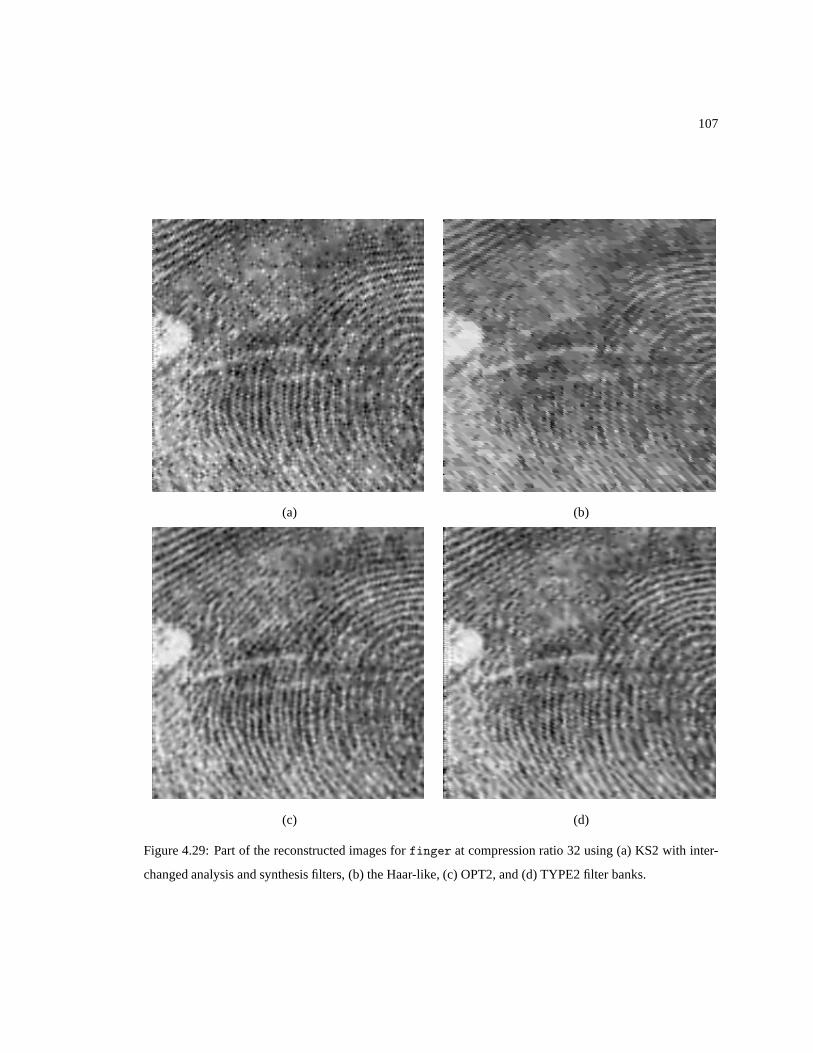
107

(a) (b)

(c) (d)

Figure 4.29: Part of the reconstructed images forfinger at compression ratio 32 using (a) KS2 with inter-

changed analysis and synthesis filters, (b) the Haar-like, (c) OPT2, and (d) TYPE2 filter banks.

finger

108

Chapter 5

Conclusions and Future Research

5.1 Conclusions

In this thesis, we have studied the design and application ofquincunx filter banks. In particular, we have

introduced symmetric extension algorithms for quincunx filter banks and proposed design methods for con-

structing high-performance quincunx filter banks for the application of image coding.

In the 1D case, the symmetric extension technique is a commonly used solution to the boundary problem

when finite-length sequences are processed. We have shown how this technique can be extended to the 2D

nonseparable quincunx case. We have examined three types ofquadrantally-centrosymmetric quincunx filter

banks, and proposed an algorithm for each type to build nonexpansive transforms of 2D sequences defined on

arbitrary rectangular regions. The type-1 algorithm can further be applied in an octave-band decomposition if

the analysis filters satisfy certain additional conditions. These schemes are potentially useful in applications

that process finite-extent sequences using quincunx filter banks.

Filter banks are highly effective for image coding applications. We have proposed three new optimization-

based techniques for the design of quincunx filter banks for image coding. The proposed design techniques

are summarized in Algorithms 4.1, 4.2, and 4.3 and yield linear-phase PR systems with high coding gain,

good analysis/synthesis filter frequency responses, and certain dual and primal vanishing moment properties.

In our design algorithms, a parametrization of quincunx filter banks based on the lifting scheme is employed

to structurally impose the PR and linear phase properties. Then, the coding gain is maximized subject to a set

of constraints on vanishing moments and frequency selectivity. Algorithm 4.1 is used to design filter banks

with two lifting steps. Algorithms 4.2 and 4.3 both work for filter banks with more than two lifting steps. In

109

Algorithm 4.2, all of the lifting filter coefficients are jointly optimized, while Algorithm 4.3 is a suboptimal

one which utilizes the first two algorithms to optimize the lifting filter coefficients in three separate steps.

It is observed that although Algorithm 4.3 yields filter banks with exact vanishing moments, in general, this

algorithm does not work as well as Algorithm 4.2. Another important observation is that Algorithm 4.2 yields

the best filter banks among all of our designs. Design examples of filter banks with all the desirable properties

were presented for each of the three techniques. These optimal filter banks were employed in an image coder

and their coding performance was compared to that of some existing quincunx and separable filter banks. The

experimental results show that our new filter banks outperform the previously proposed quincunx filter banks

for the set of JPEG-2000 test images in most cases, and sometimes these designs are even able to outperform

the 9/7 filter bank, which is considered to be one of the very best in the literature. In particular, the OPT1,

OPT3, and OPT4 filter banks consistently outperform the previously proposed quincunx filter banks for the

JPEG-2000 test images in approximately 80% of the cases. These results demonstrate the effectiveness of

our new design techniques.

5.2 Future Research

In this thesis, we focus exclusively on quincunx filter banks, which are the simplest multidimensional non-

separable filter banks. Thus, more work can be done for the general multidimensional case. For example,

symmetric extension algorithms for the face-centered-orthorhombic lattice (an extension of the quincunx lat-

tice to the three-dimensional (3D) case) would be useful fordealing with finite-extent 3D sequences. Another

example of future research in this regard is the construction of linear-phase multidimensional, multichannel,

nonseparable filter banks based on the lifting structure. Inparticular, it would be helpful to parameterize the

lifting filters such that the resulting analysis and synthesis filters have desired linear-phase properties.

In our optimal design algorithms for linear-phase PR quincunx filter banks, we assume either an isotropic

or a separable image model when maximizing the coding gain, while most images are not completely sepa-

rable or isotropic in nature. Therefore, if the separable and isotropic coding gains could be optimized jointly,

the resulting optimal filter bank may achieve better performance in image coding.

In the filter bank design algorithms, we also used a diamond-shaped passband for the ideal frequency re-

sponse. With the quincunx sampling matrix, however, the diamond shape is not the only possibility. Although

this kind of passband matches the human visual system and is desirable in image coding, in some cases, a

hexagonal- or fan-shaped passband may be more suitable. Thus, it would be useful to design quincunx filter

banks for different passband shapes.

110

The type-2 and type-3 filter banks introduced in Section 4.3.2 have antisymmetric highpass filters. As

mentioned previously, it is impossible for these filter banks to have good diamond-shaped frequency re-

sponses, thus limiting their utility for image coding. Thissaid, however, such filter banks may be advan-

tageous in other applications which employ hexagonal- or fan-shaped passband/stopband. Therefore, algo-

rithms for the design of type-2 and type-3 filter banks can be helpful for these applications.

111

Bibliography

[1] R. Ansari, H. Gaggioni, and D. G. LeGall, “HDTV coding using a nonrectangular subband decomposi-

tion,” in Proceedings of SPIE Visual Communications and Image Processing, Jan. 1988, pp. 821–824.

[2] E. Viscito and J. P. Allebach, “The analysis and design ofmultidimensional FIR perfect reconstruction

filter banks for arbitrary sampling lattices,”IEEE Transactions on Circuits and Systems, vol. 38, no. 1,

pp. 29–41, Jan. 1991.

[3] J. Kovacevic and M. Vetterli, “Nonseparable multidimensional perfect reconstruction filter banks and

wavelet bases forRn,” IEEE Transactions on Information Theory, vol. 38, no. 2, pp. 533–555, 1992.

[4] J. Kovacevic and M. Vetterli, “Nonseparable two- and three-dimensional wavelets,”IEEE Transactions

on Signal Processing, vol. 43, no. 5, pp. 1269–1273, May 1995.

[5] A. Gouze, M. Antonini, and M. Barlaud, “Quincunx liftingscheme for lossy image compression,” in

Proceedings of IEEE International Conference on Image Processing, Sept. 2000, vol. 1, pp. 665–668.

[6] J. Kovacevic and W. Sweldens, “Wavelet families of increasing order in arbitrary dimensions,”IEEE

Transactions on Image Processing, vol. 9, no. 3, pp. 480–496, Mar. 2000.

[7] S. C. Chan, K. S. Pun, and K. L. Ho, “On the design and implementation of a class of multiplierless two-

channel 1D and 2D nonseparable PR FIR filterbanks,” inProceedings of IEEE International Conference

on Image Processing, Oct. 2001, vol. 2, pp. 241–244.

[8] D. Van De Ville, T. Blu, and M. Unser, “On the multidimensional extension of the quincunx subsam-

pling matrix,” IEEE Signal Processing Letters, vol. 12, no. 2, pp. 112–115, Feb. 2005.

[9] M. Vetterli, J. Kovacevic, and D. LeGall, “Perfect reconstruction filter banks for HDTV representation

and coding,”Signal Processing: Image Communication, vol. 3, pp. 349–364, 1990.

112

[10] M. Vetterli and J Kovacevic,Wavelets and Subband Coding, Prentice Hall, Englewood Cliffs, NJ, 1995.

[11] Y. Wang, J. Ostermann, and Y.-Q. Zhang,Video Processing and Communications, Prentice-Hall,

Englewood Cliffs, NJ, USA, 2002.

[12] G. Strang and T. Nguyen,Wavelets and Filter Banks, Wellesley-Cambridge, Wellesley, MA, 1996.

[13] M. J. T. Smith and S. L. Eddins, “Subband coding images with octave band tree structures,” inPro-

ceedings of IEEE International Conference on Acoustics, Speech, and Signal Processing, Apr. 1987,

pp. 1378–1381.

[14] M. J. T. Smith and S. L. Eddins, “Analysis/synthesis techniques for subband image coding,”IEEE

Transactions on Acoustics, Speech, and Signal Processing, vol. 38, no. 8, pp. 1446–1456, Aug. 1990.

[15] S. A. Martucci, “Signal extension and noncausal filtering for subband coding of images,” inProceedings

of SPIE Visual Communications and Image Processing, Nov. 1991, vol. 1605, pp. 137–148.

[16] C. M. Brislawn, “Preservation of subband symmetry in multirate signal coding,”IEEE Transactions on

Signal Processing, vol. 43, no. 12, pp. 3046–3050, Dec. 1995.

[17] J. H. McClellan, “The design of two-dimensional digital filters by transformation,” inProc. 7th Annual

Princeton Conf. Info. Sci. and Syst., Princeton, NJ, Mar. 1973, pp. 247–251.

[18] D. B. H. Tay and N. G. Kingsbury, “Flexible design of multidimensional perfect reconstruction FIR

2-band filters using transformations of variables,”IEEE Transactions on Image Processing, vol. 2, no.

4, pp. 466–480, 1993.

[19] T. A. C. M. Kalker and I. A. Shah, “A group theoretic approach to multidimensional filter banks: Theory

and applications,”IEEE Transactions on Signal Processing, vol. 44, no. 6, pp. 1392–1405, 1996.

[20] P.P. Vaidyanathan,Multirate Systems and Filter Banks, Prentice Hall, Upper Saddle River, NJ, 1993.

[21] T. Chen and P. P. Vaidyanathan, “Multidimensional multirate filters and filter banks derived from one

dimensional filters,”IEEE Transactions on Signal Processing, vol. 41, no. 5, pp. 1749–1765, May 1993.

[22] S. M. Phoong, C. W. Kim, P. P. Vaidyanathan, and R. Ansari, “A new class of two-channel biorthogonal

filter banks and wavelet bases,”IEEE Transactions on Signal Processing, vol. 43, no. 3, pp. 649–665,

Mar. 1995.

113

[23] K. S. C. Pun and T. Q. Nguyen, “A novel and efficient designof multidimensional PR two-channel filter

banks with hourglass-shaped passband support,”IEEE Signal Processing Letters, vol. 11, no. 3, pp.

345–348, Mar. 2004.

[24] G. Karlsson and M. Vetterli, “Theory of two-dimensional multirate filter banks,”IEEE Transactions on

Acoustics, Speech, and Signal Processing, vol. 38, no. 6, pp. 925 – 937, 1990.

[25] T. D. Tran, R. L. de Queiroz, and T. Q. Nguyen, “Linear-phase perfect reconstruction filter bank: Lattice

structure, design, and application in image coding,”IEEE Transactions on Signal Processing, vol. 48,

no. 1, pp. 133–147, Jan. 2000.

[26] W. Sweldens, “The lifting scheme: A custom-design construction of biorthogonal wavelets,”Applied

and Computational Harmonic Analysis, vol. 3, pp. 186–200, 1996.

[27] I. Daubechies and W. Sweldens, “Factoring wavelet transforms into lifting steps,” .

[28] T. Cooklev, A. Nishihara, T. Yoshida, and M. Sablatash,“Multidimensional two-channel linear phase

FIR filter banks and wavelet bases with vanishing moments,”Journal of Multidimensional Systems and

Signal Processing, vol. 9, pp. 39–76, Jan. 1998.

[29] D. E. Dudgeon and R. M. Mersereau,Multidimensional Digital Signal Processing, Prentice-Hall,

Englewood Cliffs, NJ, USA, 1984.

[30] S. G. Mallat, “A theory of multiresolution signal decomposition: The wavelet representation,”IEEE

Transactions on Pattern Analysis and Machine Intelligence, vol. 11, no. 7, pp. 674–693, 1989.

[31] O. Rioul, “A discrete-time multiresolution theory,”IEEE Transactions on Signal Processing, vol. 41,

no. 8, pp. 2591–2606, Aug. 1993.

[32] S. G. Mallat, “Multifrequency channel decompositionsof images and wavelet models,”IEEE Transac-

tions on Acoustics, Speech, and Signal Processing, vol. 37, no. 12, pp. 2091–2110, Dec. 1989.

[33] A. R. Calderbank, I. Daubechies, W. Sweldens, and B.-L.Yeo, “Wavelet transforms that map integers

to integers,”Applied and Computational Harmonic Analysis, vol. 5, no. 3, pp. 332–369, July 1998.

[34] J. Katto and Y. Yasuda, “Performance evaluation of subband coding and optimization of its filter coef-

ficients,” inProceedings of SPIE Visual Communications and Image Processing, Nov. 1991, vol. 1605,

pp. 95–106.

114

[35] E. A. B. da Silva, Wavelet Transforms for Image Coding, Ph.D. thesis, Department of Electronic

Systems Engineering, University of Essex, UK, 1995.

[36] Y. Chen, M. D. Adams, and W.-S. Lu, “Symmetric extensionfor quincunx filter banks,” inProceedings

of IEEE Pacific Rim Conference on Communications, Computersand Signal Processing, Aug. 2005,

pp. 542–545.

[37] Y. Chen, M. D. Adams, and W.-S. Lu, “Symmetric extensionfor two-channel quincunx filter banks,” in

Proceedings of IEEE International Conference on Image Processing, Sept. 2005, vol. 1, pp. 461–464.

[38] S. Coulombe and E. Dubois, “Linear phase and symmetriesfor multidimensional FIR filters over

lattices,” IEEE Transactions on Circuits and Systems—II: Analog and Digital Signal Processing, vol.

45, no. 4, pp. 473–481, Apr. 1998.

[39] Y. Chen, M. D. Adams, and W.-S. Lu, “Design of optimal quincunx filter banks for image coding,” in

Proceedings of IEEE International Symposium on Circuits and Systems, May 2006, to appear.

[40] ISO/IEC 15444-1: Information technology—JPEG 2000 image coding system—Part 1: Core coding

system, 2000.

[41] M. S. Lobo, L. Vandenberghe, S. Boyd, and H. Lebret, “Applications of second-order cone program-

ming,” Linear Algebra and Applications, vol. 284, pp. 193–228, Nov. 1998.

[42] J.F. Sturm, “Using SeDuMi 1.02, a MATLAB toolbox for optimization over symmetric cones,”Opti-

mization Methods and Software, vol. 11–12, pp. 625–653, 1999.

[43] M. D. Adams, “ELEC 545 project: A wavelet-based lossy/lossless image compression system,” Dept.

of Electrical and Computer Engineering, University of British Columbia, Vancouver, BC, Canada, Apr.

1999.

[44] “JPEG-2000 test images,” ISO/IEC JTC 1/SC 29/WG 1 N 545,July 1997.

UNIVERSITY OF VICTORIA PARTIAL COPYRIGHT LICENSE

I hereby grant the right to lend my thesis to users of the University of Victoria Library, and to make single

copies only for such users or in response to a request from theLibrary of any other university, or similar

institution, on its behalf or for one of its users. I further agree that permission for extensive copying of this

thesis for scholarly purposes may be granted by me or a memberof the University designated by me. It is

understood that copying or publication of this thesis for financial gain by the University of Victoria shall not

be allowed without my written permission.

Title of Thesis:

Design and Application of Quincunx Filter Banks

Author

Yi Chen

Signed: May 15, 2006

design and application of quincunx filter banksfrodo/publications/ychen_mascthesis.pdf · design...

Documents