design and analysis of mac protocols for wireless networks
TRANSCRIPT
Graduate Theses and Dissertations Iowa State University Capstones, Theses andDissertations
2009
Design and analysis of MAC protocols for wirelessnetworksHaithem Al-meflehIowa State University
Follow this and additional works at: https://lib.dr.iastate.edu/etd
Part of the Electrical and Computer Engineering Commons
This Dissertation is brought to you for free and open access by the Iowa State University Capstones, Theses and Dissertations at Iowa State UniversityDigital Repository. It has been accepted for inclusion in Graduate Theses and Dissertations by an authorized administrator of Iowa State UniversityDigital Repository. For more information, please contact [email protected].
Recommended CitationAl-mefleh, Haithem, "Design and analysis of MAC protocols for wireless networks" (2009). Graduate Theses and Dissertations. 12210.https://lib.dr.iastate.edu/etd/12210
Design and analysis of MAC protocols for wireless networks
by
Haithem Abdel-Razaq Ahmad Al-Mefleh
A dissertation submitted to the graduate faculty
in partial fulfillment of the requirements for the degree of
DOCTOR OF PHILOSOPHY
Major: Computer Engineering
Program of Study Committee:J. Morris Chang, Major Professor
Ahmed E. KamalDaji Qiao
Zhao ZhangLu Ruan
Iowa State University
Ames, Iowa
2009

ii
DEDICATION
To my parents.

iii
TABLE OF CONTENTS
LIST OF TABLES . . . . . . . . . . . . . . . . . . . . . . . . . . . . . . . . . . . vii
LIST OF FIGURES . . . . . . . . . . . . . . . . . . . . . . . . . . . . . . . . . . viii
ACKNOWLEDGEMENTS . . . . . . . . . . . . . . . . . . . . . . . . . . . . . . xii
ABSTRACT . . . . . . . . . . . . . . . . . . . . . . . . . . . . . . . . . . . . . . . xiii
CHAPTER 1. Introduction . . . . . . . . . . . . . . . . . . . . . . . . . . . . . 1
1.1 IEEE 802.11 . . . . . . . . . . . . . . . . . . . . . . . . . . . . . . . . . . . . . . 1
1.2 IEEE 802.16 . . . . . . . . . . . . . . . . . . . . . . . . . . . . . . . . . . . . . . 6
1.3 Organization . . . . . . . . . . . . . . . . . . . . . . . . . . . . . . . . . . . . . 7
CHAPTER 2. The Design and Analysis of a High-Performance Distributed
Coordination Function for IEEE 802.11 Wireless Networks . . . . . . . . 8
2.1 Abstract . . . . . . . . . . . . . . . . . . . . . . . . . . . . . . . . . . . . . . . . 8
2.2 Introduction . . . . . . . . . . . . . . . . . . . . . . . . . . . . . . . . . . . . . . 9
2.3 Related Work . . . . . . . . . . . . . . . . . . . . . . . . . . . . . . . . . . . . . 11
2.4 HDCF Details . . . . . . . . . . . . . . . . . . . . . . . . . . . . . . . . . . . . . 12
2.4.1 Definitions . . . . . . . . . . . . . . . . . . . . . . . . . . . . . . . . . . 12
2.4.2 Next-Station Selection . . . . . . . . . . . . . . . . . . . . . . . . . . . . 13
2.4.3 Announcement . . . . . . . . . . . . . . . . . . . . . . . . . . . . . . . . 14
2.4.4 HDCF Rules . . . . . . . . . . . . . . . . . . . . . . . . . . . . . . . . . 15
2.4.5 An Example . . . . . . . . . . . . . . . . . . . . . . . . . . . . . . . . . 18
2.4.6 Recovery Mechanism . . . . . . . . . . . . . . . . . . . . . . . . . . . . . 19
2.4.7 Summary, and Advantages . . . . . . . . . . . . . . . . . . . . . . . . . 20

iv
2.5 Performance Analysis . . . . . . . . . . . . . . . . . . . . . . . . . . . . . . . . 20
2.5.1 How to Handle New Arrivals . . . . . . . . . . . . . . . . . . . . . . . . 21
2.5.2 How Contentions Are Resolved . . . . . . . . . . . . . . . . . . . . . . . 23
2.5.3 Maximum Achieved Throughput . . . . . . . . . . . . . . . . . . . . . . 25
2.5.4 Packets Transmission Differences . . . . . . . . . . . . . . . . . . . . . . 25
2.5.5 Approximate Analysis . . . . . . . . . . . . . . . . . . . . . . . . . . . . 26
2.6 Simulation . . . . . . . . . . . . . . . . . . . . . . . . . . . . . . . . . . . . . . . 27
2.6.1 Performance Metrics . . . . . . . . . . . . . . . . . . . . . . . . . . . . . 27
2.6.2 Saturated Stations . . . . . . . . . . . . . . . . . . . . . . . . . . . . . . 28
2.6.3 Non-saturated stations, CBR Traffic . . . . . . . . . . . . . . . . . . . . 30
2.6.4 Non-saturated stations, VBR Traffic . . . . . . . . . . . . . . . . . . . . 33
2.6.5 Channel Noise . . . . . . . . . . . . . . . . . . . . . . . . . . . . . . . . 36
2.7 Conclusions . . . . . . . . . . . . . . . . . . . . . . . . . . . . . . . . . . . . . . 37
CHAPTER 3. A New ACK Policy To Mitigate the Effects of Coexisting
IEEE 802.11/802.11e Devices . . . . . . . . . . . . . . . . . . . . . . . . . . 38
3.1 Abstract . . . . . . . . . . . . . . . . . . . . . . . . . . . . . . . . . . . . . . . . 38
3.2 Introduction . . . . . . . . . . . . . . . . . . . . . . . . . . . . . . . . . . . . . . 39
3.3 IEEE 802.11 Background . . . . . . . . . . . . . . . . . . . . . . . . . . . . . . 42
3.3.1 Distributed Coordination Function (DCF) . . . . . . . . . . . . . . . . . 42
3.3.2 Enhanced Distributed Channel Access (EDCA) . . . . . . . . . . . . . . 43
3.4 IEEE 802.11 DCF/EDCA Coexistence . . . . . . . . . . . . . . . . . . . . . . . 44
3.4.1 Problem Statement . . . . . . . . . . . . . . . . . . . . . . . . . . . . . . 44
3.4.2 Desirable Features . . . . . . . . . . . . . . . . . . . . . . . . . . . . . . 45
3.5 Related Work . . . . . . . . . . . . . . . . . . . . . . . . . . . . . . . . . . . . . 46
3.6 NZ-ACK Details . . . . . . . . . . . . . . . . . . . . . . . . . . . . . . . . . . . 48
3.6.1 An Overview . . . . . . . . . . . . . . . . . . . . . . . . . . . . . . . . . 48
3.6.2 Operations of NZ-ACK . . . . . . . . . . . . . . . . . . . . . . . . . . . 50
3.6.3 When to Issue NZ-ACK Frames . . . . . . . . . . . . . . . . . . . . . . 51

v
3.6.4 How Long is the Duration of an NZ-ACK Frame . . . . . . . . . . . . . 52
3.6.5 Implementation . . . . . . . . . . . . . . . . . . . . . . . . . . . . . . . . 53
3.7 Evaluation . . . . . . . . . . . . . . . . . . . . . . . . . . . . . . . . . . . . . . . 54
3.7.1 Performance Metrics . . . . . . . . . . . . . . . . . . . . . . . . . . . . . 55
3.7.2 Saturated Network . . . . . . . . . . . . . . . . . . . . . . . . . . . . . . 55
3.7.3 Non-saturated Networks . . . . . . . . . . . . . . . . . . . . . . . . . . . 58
3.8 Conclusions . . . . . . . . . . . . . . . . . . . . . . . . . . . . . . . . . . . . . . 60
CHAPTER 4. Turning Hidden Nodes into Helper Nodes in IEEE 802.11
Wireless LAN Networks . . . . . . . . . . . . . . . . . . . . . . . . . . . . . 62
4.1 Abstract . . . . . . . . . . . . . . . . . . . . . . . . . . . . . . . . . . . . . . . . 62
4.2 Introduction . . . . . . . . . . . . . . . . . . . . . . . . . . . . . . . . . . . . . . 62
4.3 Background . . . . . . . . . . . . . . . . . . . . . . . . . . . . . . . . . . . . . . 63
4.3.1 IEEE 802.11 DCF . . . . . . . . . . . . . . . . . . . . . . . . . . . . . . 64
4.3.2 Hidden Terminal Problem . . . . . . . . . . . . . . . . . . . . . . . . . . 65
4.4 Related Work . . . . . . . . . . . . . . . . . . . . . . . . . . . . . . . . . . . . . 66
4.5 The Proposed Scheme . . . . . . . . . . . . . . . . . . . . . . . . . . . . . . . . 67
4.5.1 Motivation . . . . . . . . . . . . . . . . . . . . . . . . . . . . . . . . . . 67
4.5.2 Description of the New Scheme . . . . . . . . . . . . . . . . . . . . . . . 68
4.5.3 Capture Effect . . . . . . . . . . . . . . . . . . . . . . . . . . . . . . . . 70
4.5.4 Implementation Issues . . . . . . . . . . . . . . . . . . . . . . . . . . . . 70
4.6 Analysis . . . . . . . . . . . . . . . . . . . . . . . . . . . . . . . . . . . . . . . . 71
4.6.1 Channel State . . . . . . . . . . . . . . . . . . . . . . . . . . . . . . . . 71
4.6.2 Throughput and Throughput Gain . . . . . . . . . . . . . . . . . . . . . 72
4.6.3 Throughput Analysis . . . . . . . . . . . . . . . . . . . . . . . . . . . . . 74
4.6.4 Phelp,n, and Phelp,m . . . . . . . . . . . . . . . . . . . . . . . . . . . . . . 77
4.7 Performance Evaluation . . . . . . . . . . . . . . . . . . . . . . . . . . . . . . . 80
4.7.1 Performance Metrics . . . . . . . . . . . . . . . . . . . . . . . . . . . . . 80
4.7.2 Hidden Groups without Capture Effect . . . . . . . . . . . . . . . . . . 81
vi
4.7.3 Analysis Model Validation . . . . . . . . . . . . . . . . . . . . . . . . . . 86
4.7.4 Random Scenario with Capture Effect . . . . . . . . . . . . . . . . . . . 88
4.8 Conclusions . . . . . . . . . . . . . . . . . . . . . . . . . . . . . . . . . . . . . . 89
CHAPTER 5. Maintaining Priority among IEEE 802.11/802.11e Devices . 90
5.1 Introduction . . . . . . . . . . . . . . . . . . . . . . . . . . . . . . . . . . . . . . 90
5.2 Analysis . . . . . . . . . . . . . . . . . . . . . . . . . . . . . . . . . . . . . . . . 91
5.3 Evaluation . . . . . . . . . . . . . . . . . . . . . . . . . . . . . . . . . . . . . . . 98
5.3.1 Performance Metrics . . . . . . . . . . . . . . . . . . . . . . . . . . . . . 99
5.3.2 Saturated Network . . . . . . . . . . . . . . . . . . . . . . . . . . . . . . 99
5.3.3 Non-Saturated Network . . . . . . . . . . . . . . . . . . . . . . . . . . . 101
5.4 Conclusions . . . . . . . . . . . . . . . . . . . . . . . . . . . . . . . . . . . . . . 102
CHAPTER 6. Enhancing Bandwidth Utilization for the IEEE 802.16e . . . 105
6.1 Abstract . . . . . . . . . . . . . . . . . . . . . . . . . . . . . . . . . . . . . . . . 105
6.2 Introduction . . . . . . . . . . . . . . . . . . . . . . . . . . . . . . . . . . . . . . 106
6.3 An Overview of the IEEE 802.16 MAC . . . . . . . . . . . . . . . . . . . . . . . 108
6.4 Related Work . . . . . . . . . . . . . . . . . . . . . . . . . . . . . . . . . . . . . 110
6.5 Details of the Proposed Solution . . . . . . . . . . . . . . . . . . . . . . . . . . 113
6.5.1 Problem Statement . . . . . . . . . . . . . . . . . . . . . . . . . . . . . . 113
6.5.2 Description . . . . . . . . . . . . . . . . . . . . . . . . . . . . . . . . . . 114
6.5.3 Utilization . . . . . . . . . . . . . . . . . . . . . . . . . . . . . . . . . . . 115
6.5.4 Algorithm at BS . . . . . . . . . . . . . . . . . . . . . . . . . . . . . . . 117
6.6 Simulation . . . . . . . . . . . . . . . . . . . . . . . . . . . . . . . . . . . . . . . 119
6.6.1 Traffic Characteristics . . . . . . . . . . . . . . . . . . . . . . . . . . . . 120
6.6.2 Performance Metrics . . . . . . . . . . . . . . . . . . . . . . . . . . . . . 120
6.6.3 Results . . . . . . . . . . . . . . . . . . . . . . . . . . . . . . . . . . . . 122
6.7 Conclusions . . . . . . . . . . . . . . . . . . . . . . . . . . . . . . . . . . . . . . 126
CHAPTER 7. Conclusions and Future Work . . . . . . . . . . . . . . . . . . 127
BIBLIOGRAPHY . . . . . . . . . . . . . . . . . . . . . . . . . . . . . . . . . . . 132

vii
LIST OF TABLES
Table 2.1 Network Parameters . . . . . . . . . . . . . . . . . . . . . . . . . . . . 28
Table 3.1 Saturation Results - 1 . . . . . . . . . . . . . . . . . . . . . . . . . . . 56
Table 3.2 Saturation Results - 2 . . . . . . . . . . . . . . . . . . . . . . . . . . . 56
Table 4.1 Network Parameters . . . . . . . . . . . . . . . . . . . . . . . . . . . . 80
Table 6.1 Poll/grant options for each scheduling service (37; 38) . . . . . . . . . 111
Table 6.2 IEEE 802.16 Network Parameters . . . . . . . . . . . . . . . . . . . . . 121

viii
LIST OF FIGURES
Figure 2.1 Probability of collision in DCF . . . . . . . . . . . . . . . . . . . . . . 9
Figure 2.2 MAC frame format . . . . . . . . . . . . . . . . . . . . . . . . . . . . . 14
Figure 2.3 Frame Control field . . . . . . . . . . . . . . . . . . . . . . . . . . . . . 14
Figure 2.4 Active transmissions and their components . . . . . . . . . . . . . . . . 15
Figure 2.5 Basic operation of DCF . . . . . . . . . . . . . . . . . . . . . . . . . . 16
Figure 2.6 The interrupt scheme . . . . . . . . . . . . . . . . . . . . . . . . . . . . 17
Figure 2.7 An example with three stations joining network at different times . . . 18
Figure 2.8 Recovery from a lost announcement . . . . . . . . . . . . . . . . . . . . 19
Figure 2.9 New arrivals effect on contention level . . . . . . . . . . . . . . . . . . 22
Figure 2.10 Probability of collision comparison . . . . . . . . . . . . . . . . . . . . 23
Figure 2.11 Different modes of transmissions . . . . . . . . . . . . . . . . . . . . . . 26
Figure 2.12 Throughput vs. packet size . . . . . . . . . . . . . . . . . . . . . . . . 29
Figure 2.13 Throughput vs. network size . . . . . . . . . . . . . . . . . . . . . . . . 29
Figure 2.14 Minimum and maximum gain of throughput . . . . . . . . . . . . . . . 30
Figure 2.15 Fairness Index for 1 second period . . . . . . . . . . . . . . . . . . . . . 31
Figure 2.16 Fairness Index for 3 seconds period . . . . . . . . . . . . . . . . . . . . 31
Figure 2.17 Throughput vs. load, 802.11b . . . . . . . . . . . . . . . . . . . . . . . 32
Figure 2.18 Throughput vs. load, 802.11g . . . . . . . . . . . . . . . . . . . . . . . 32
Figure 2.19 Throughput vs. number of users, 802.11b . . . . . . . . . . . . . . . . . 32
Figure 2.20 Throughput vs. number of users, 802.11g . . . . . . . . . . . . . . . . . 33
Figure 2.21 Fairness Index vs. time . . . . . . . . . . . . . . . . . . . . . . . . . . . 33
Figure 2.22 Network with VBR traffic, 802.11b . . . . . . . . . . . . . . . . . . . . 34

ix
Figure 2.23 Network with VBR traffic, 802.11g . . . . . . . . . . . . . . . . . . . . 34
Figure 2.24 Network with both CBR and VBR traffic, 802.11b . . . . . . . . . . . 35
Figure 2.25 Network with both CBR and VBR traffic, 802.11g . . . . . . . . . . . 35
Figure 2.26 Throughput vs. noise level, 802.11g . . . . . . . . . . . . . . . . . . . . 36
Figure 3.1 EDCA Transmission Queues and EDCAFs . . . . . . . . . . . . . . . . 44
Figure 3.2 Interframe Space Relations . . . . . . . . . . . . . . . . . . . . . . . . . 44
Figure 3.3 Virtual real-time queues at the QAP . . . . . . . . . . . . . . . . . . . 45
Figure 3.4 An example of NZ-ACK operation with a transmission of two fragments 49
Figure 3.5 Frame Control field . . . . . . . . . . . . . . . . . . . . . . . . . . . . . 53
Figure 3.6 Throughput . . . . . . . . . . . . . . . . . . . . . . . . . . . . . . . . . 57
Figure 3.7 Retransmission attempts . . . . . . . . . . . . . . . . . . . . . . . . . . 58
Figure 3.8 Packet Delay, CDF . . . . . . . . . . . . . . . . . . . . . . . . . . . . . 59
Figure 3.9 Packet Delay . . . . . . . . . . . . . . . . . . . . . . . . . . . . . . . . 60
Figure 4.1 RTS/CTS operation without hidden nodes . . . . . . . . . . . . . . . . 65
Figure 4.2 Hidden terminal problem . . . . . . . . . . . . . . . . . . . . . . . . . . 65
Figure 4.3 Collision due to hidden terminal problem . . . . . . . . . . . . . . . . . 65
Figure 4.4 The proposed scheme . . . . . . . . . . . . . . . . . . . . . . . . . . . . 69
Figure 4.5 ACK frame . . . . . . . . . . . . . . . . . . . . . . . . . . . . . . . . . 70
Figure 4.6 CACK frame . . . . . . . . . . . . . . . . . . . . . . . . . . . . . . . . 70
Figure 4.7 Channel state . . . . . . . . . . . . . . . . . . . . . . . . . . . . . . . . 71
Figure 4.8 Success and collision times in DCF with RTS-CTS . . . . . . . . . . . 72
Figure 4.9 Success and collision times in DCF with RTS-CTS when the new scheme
is enabled . . . . . . . . . . . . . . . . . . . . . . . . . . . . . . . . . . 72
Figure 4.10 Two groups of hidden nodes . . . . . . . . . . . . . . . . . . . . . . . . 75
Figure 4.11 Time during which a collision due to hidden stations may occur . . . . 76
Figure 4.12 Markove chain model . . . . . . . . . . . . . . . . . . . . . . . . . . . . 77
Figure 4.13 Scenario 1-m . . . . . . . . . . . . . . . . . . . . . . . . . . . . . . . . . 82

x
Figure 4.14 Scenario 2-m . . . . . . . . . . . . . . . . . . . . . . . . . . . . . . . . . 82
Figure 4.15 Scenario 3-m . . . . . . . . . . . . . . . . . . . . . . . . . . . . . . . . . 82
Figure 4.16 Scenario 5-m . . . . . . . . . . . . . . . . . . . . . . . . . . . . . . . . . 83
Figure 4.17 Scenario 10-m . . . . . . . . . . . . . . . . . . . . . . . . . . . . . . . . 83
Figure 4.18 Scenario 1-m-c . . . . . . . . . . . . . . . . . . . . . . . . . . . . . . . . 84
Figure 4.19 Scenario 2-m-c . . . . . . . . . . . . . . . . . . . . . . . . . . . . . . . . 84
Figure 4.20 Delay . . . . . . . . . . . . . . . . . . . . . . . . . . . . . . . . . . . . . 84
Figure 4.21 Retransmissions . . . . . . . . . . . . . . . . . . . . . . . . . . . . . . . 85
Figure 4.22 Packet drop . . . . . . . . . . . . . . . . . . . . . . . . . . . . . . . . . 85
Figure 4.23 Scenario 1-m . . . . . . . . . . . . . . . . . . . . . . . . . . . . . . . . . 86
Figure 4.24 Scenario 2-m . . . . . . . . . . . . . . . . . . . . . . . . . . . . . . . . . 87
Figure 4.25 Scenario 3-m . . . . . . . . . . . . . . . . . . . . . . . . . . . . . . . . . 87
Figure 4.26 Scenario 5-m . . . . . . . . . . . . . . . . . . . . . . . . . . . . . . . . . 87
Figure 4.27 Scenario 10-m . . . . . . . . . . . . . . . . . . . . . . . . . . . . . . . . 88
Figure 4.28 Performance gain for random scenario with capture effect . . . . . . . 89
Figure 5.1 Expected CWmin . . . . . . . . . . . . . . . . . . . . . . . . . . . . . . 92
Figure 5.2 Channel access after an ACK with AIFS=DIFS . . . . . . . . . . . . . 93
Figure 5.3 Channel access after an ACK with AIFS>DIFS . . . . . . . . . . . . . 93
Figure 5.4 Throughput Disabled; 5 EDCA, 1 DCF . . . . . . . . . . . . . . . . . . 96
Figure 5.5 Throughput Enabled; 5 EDCA, 1 DCF . . . . . . . . . . . . . . . . . 96
Figure 5.6 Throughput Disabled; 5 EDCA, 50 DCF . . . . . . . . . . . . . . . . . 97
Figure 5.7 Throughput Enabled; 5 EDCA, 50 DCF . . . . . . . . . . . . . . . . . 97
Figure 5.8 Delay; 5 EDCA, 1 DCF . . . . . . . . . . . . . . . . . . . . . . . . . . 97
Figure 5.9 Delay; 5 EDCA, 50 DCF . . . . . . . . . . . . . . . . . . . . . . . . . . 98
Figure 5.10 Throughput v.s. number of DCF users; 5 EDCA . . . . . . . . . . . . 100
Figure 5.11 Throughput v.s. number of DCF users; 10 EDCA . . . . . . . . . . . . 100
Figure 5.12 Delay v.s. number of DCF users; 5,10 EDCA . . . . . . . . . . . . . . 100
Figure 5.13 Fairness Index v.s. number of DCF users . . . . . . . . . . . . . . . . . 101

xi
Figure 5.14 Throughput; 15 EDCA - on-off model . . . . . . . . . . . . . . . . . . . 102
Figure 5.15 Delay; 15 EDCA - on-off model . . . . . . . . . . . . . . . . . . . . . . 102
Figure 6.1 An example of IEEE 802.16 frame structure with TDD . . . . . . . . . 108
Figure 6.2 ON-OFF Model . . . . . . . . . . . . . . . . . . . . . . . . . . . . . . . 116
Figure 6.3 Network topology . . . . . . . . . . . . . . . . . . . . . . . . . . . . . . 120
Figure 6.4 Throughput - 2 ertps SSs . . . . . . . . . . . . . . . . . . . . . . . . . . 122
Figure 6.5 Delay and jitter - 2 ertps SSs . . . . . . . . . . . . . . . . . . . . . . . 123
Figure 6.6 Throughput - 4 ertps SSs . . . . . . . . . . . . . . . . . . . . . . . . . . 124
Figure 6.7 Delay ertps - 4 ertps SSs . . . . . . . . . . . . . . . . . . . . . . . . . . 124
Figure 6.8 Throughput BE - 4 BE SSs . . . . . . . . . . . . . . . . . . . . . . . . 125
Figure 6.9 Delay ertps - 4 BE SSs . . . . . . . . . . . . . . . . . . . . . . . . . . . 125

xii
ACKNOWLEDGEMENTS
I would like to express my thanks to those who helped me with various aspects of conducting
research and the writing of this thesis. First and foremost, Dr. Morris Chang, my supervisor,
for his guidance and support throughout this research and the writing of this thesis. I would
like also to thank my committee members for their efforts and contributions to this work: Dr.
Ahmed E. Kamal, Dr. Daji Qiao, Dr. Zhao Zhang, and Dr. Lu Ruan. Finally, I would like to
thank my family, friends, and everyone who helped me during my study period.

xiii
ABSTRACT
During the last few years, wireless networking has attracted much of the research and
industry interest. In addition, almost all current wireless devices are based on the IEEE
802.11 and IEEE 802.16 standards for the local and metropolitan area networks (LAN/MAN)
respectively. Both of these standards define the medium access control layer (MAC) and
physical layer (PHY) parts of a wireless user. In a wireless network, the MAC protocol plays
a significant role in determining the performance of the whole network and individual users.
Accordingly, many challenges are addressed by research to improve the performance of MAC
operations in IEEE 802.11 and IEEE 802.16 standards. Such performance is measured using
different metrics like the throughput, fairness, delay, utilization, and drop rate.
We propose new protocols and solutions to enhance the performance of an IEEE 802.11
WLAN (wireless LAN) network, and to enhance the utilization of an IEEE 802.16e WMAN
(wireless MAN). First, we propose a new protocol called HDCF (High-performance Distributed
Coordination Function), to address the problem of wasted time, or idle slots and collided
frames, in contention resolution of the IEEE 802.11 DCF. Second, we propose a simple pro-
tocol that enhances the performance of DCF in the existence of the hidden terminal problem.
Opposite to other approaches, the proposed protocol attempts to benefit from the hidden ter-
minal problem. Third, we propose two variants of a simple though effective distributed scheme,
called NZ-ACK (Non Zero-Acknowledgement), to address the effects of coexisting IEEE 802.11e
EDCA and IEEE 802.11 DCF devices. Finally, we investigate encouraging ertPS (enhanced
real time Polling Service) connections, in an IEEE 802.16e, network to benefit from contention,
and we aim at improving the network performance without violating any delay requirements
of voice applications.

1
CHAPTER 1. Introduction
During the last few years, wireless networking has attracted much of the research and
industry interest. In addition, almost all current wireless devices are based on the IEEE
802.11 and IEEE 802.16 standards for the local and metropolitan area networks (LAN/MAN)
respectively. Both of these standards define the medium access control layer (MAC) and
physical layer (PHY) parts of a wireless user.
In a wireless network, the MAC protocol plays a significant role in determining the perfor-
mance of the whole network and individual users. Accordingly, many challenges are addressed
by research to improve the performance of MAC operations in IEEE 802.11 and IEEE 802.16
standards. Such performance is measured using different metrics like the throughput, fairness,
delay, utilization, and drop rate.
1.1 IEEE 802.11
The 802.11 standard defines two modes of operation: DCF (Distributed Coordination Func-
tion), and PCF (Point Coordination Function). Alternatively, the new Hybrid Coordination
Function (HCF) is introduced in the 802.11e standard to provide different mechanisms to meet
the growing demand of users for real-time application. HCF includes two modes of operation:
Enhanced Distributed Coordination Access (EDCA), and HCF Controlled Access (HCCA).
PCF and HCCA are centralized controlled access methods that exist at a coordinator node,
the access point (AP). The AP uses polling to assign the right to access the channel following a
predetermined schedule. Both operations have the drawbacks of requiring a coordinator node,
and adding the overhead of polling messages that are usually transmitted using lower physical
rates. On the other hand, DCF and EDCA are distributed contention-based access functions

2
in which the right to access the wireless channel is determined by different local contention
parameters used by every user. Extending DCF, EDCA introduces different QoS (quality of
service) mechanisms like priority levels and transmission time bounds. Consequently, much
attention is given to the distributed operations of IEEE 802.11 especially DCF which is the
basic operation of the MAC protocol defined in all IEEE 802.11 standards including the IEEE
802.11e.
Using the IEEE 802.11 DCF, stations compete for the channel using a random backoff
access scheme. Therefore, there is an overhead of idle slots and collisions which degrade the
performance of DCF. Such degradation increases with higher loads and network sizes, and with
the existence of hidden terminal problem. In addition, wireless networks are expected to have
a mix of IEEE 802.11 and IEEE 802.11e standards. Hence, there has been an interest in the
performance of such networks due to the deference between EDCA and legacy DCF.
We propose new protocols and solutions to enhance the performance of an IEEE 802.11
WLAN (wireless LAN) network. First, we propose a new protocol called HDCF (High-
performance DCF), to address the problem of wasted time, or idle slots and collided frames, in
contention resolution of DCF. Second, we propose a simple protocol that enhances the perfor-
mance of DCF in the existence of the hidden terminal problem. Opposite to other approaches,
the proposed protocol attempts to benefit from the hidden terminal problem. Finally, we
propose two variants of a simple though effective distributed scheme, called NZ-ACK (Non
Zero-Acknowledgement), to address the effects of coexisting IEEE 802.11e EDCA and IEEE
802.11 DCF devices.
We implemented all of these proposed protocols using Opnet Modeler by modifying the
existing 802.11/802.11e models which represent the MAC and PHY layers. In addition, the
wireless medium is presented via a number of pipeline stages. These stages allow for determin-
ing propagation delays, transmission ranges, out of range stations, and different properties of
all transmitted and received signals (like SNR and power). We modified some of these stages
to add the capture effect feature and the hidden terminal problem.

3
High-Performance Distributed Coordination Function (HDCF)
The performance of 802.11 DCF degrades especially under larger network sizes, and higher
loads due to higher contention level resulting in more idle slots and higher collision rates.
We propose HDCF to address the problem of wasted time in contention resolution of DCF via
classifying stations into active and inactive ones. The objectives are to coordinate transmissions
from different active stations with no collisions or idle slots, and limit the contention to newly
transmitting stations. HDCF utilizes an interrupt scheme with active transmissions to enhance
the fairness and eliminate, or reduce much of, the costs of contention in DCF (idle slots and
collisions) without adding any assumptions or constraints to DCF.
We provide a simple analytical description of HDCF compared to DCF. We use a simple but
a well-known and an accurate model of the IEEE DCF which is presented in (2), and we start
with assumptions like that used in (2). We explain how new arrivals affect the probability of
collision, and how the collision level is reduced. We also show that like DCF, HDCF operation
consists of cycles such that each cycle includes on average a transmission by each user in the
network. While DCF achieves this fairness property with the cost of idle slots and collisions,
HDCF reduces much of such overheads, and thus is expected to enhance the throughput and
fairness of the network.
In general, HDCF has the following advantages: 1) No idle slots wasted when there are
no new stations trying to transmit, or no need to stop active transmissions. 2) Fairness to
new stations as they can contend for the channel directly (like in DCF) without long delays as
the contention cost is much smaller. 3) Stations transmit in random order without the need
for a slotted channel, reserved periods, time synchronization, central control, or knowledge of
number of active users.
Finally, we use Opnet to provide a simulation study for networks of two different PHYs
(the IEEE 802.11b and 802.11g). In addition, the experiments consider different loads, network
sizes (number of users in the network), noise levels, packet sizes, and traffic types. Results
illustrate that HDCF outperforms DCF with gains up to 391.2% of throughput and 26.8% of
fairness level.

4
Taking Advantage of the Existence of Hidden Nodes
When wireless users are out of range, they would not be able to hear frames transmitted
by each other. This is referred to as the hidden terminal problem, and significantly degrades
the performance of the IEEE 802.11 DCF because it results in higher collision rates.
Although the problem is addressed by different works, it is not totally eliminated. Hence,
we propose a simple protocol that enhances the performance of DCF in the existence of hidden
terminal problem. Opposite to other approaches, we propose to take advantage of the hidden
terminal problem whenever possible. We investigate if non-hidden stations could help each
other retransmit faster to enhance the performance of 802.11 WLANs. Such cooperative re-
transmissions are expected to be faster since with DCF a non-collided station mostly transmits
earlier than collided stations that double their backoff values. The proposed scheme modifies
802.11 DCF, is backward compatible, and works over the 802.11 PHY. We also present an
analysis model to calculate the saturation throughput of the new scheme and compare it to
that of DCF.
Capture effect is an advancement in wireless networks that allows a station to correctly
receive one of the collided frames under some conditions like a threshold of the received signal’s
SNR (signal-to-noise ratio). Thus, captures would enhance the throughout of the network while
decreasing the fairness level. Consequently, we consider capture effect as it may reduce the
gains of the proposed scheme, and would make it possible for the new scheme to be used even
in a fully-connected WLAN where there are no hidden nodes.
Using Opnet simulation, we evaluate the new scheme with and without the capture effect
for different topologies. Results show gains of the number of retransmissions per packet,
throughput, fairness, delay, and packet drops. However, there is a small trade-off regarding
fairness in some scenarios. Finally, simulation is used to validate the analytical model.
Non-Zero ACK (NZ-ACK)
The 802.11e standard is designed to be backward compatible with the 802.11. Thus wireless
networks are expected to have mix of EDCA (802.11e) and legacy DCF (802.11, 802.11b,

5
802.11g, and 802.11a) users. As a result, EDCA users’ performance may be degraded because
of the existence of legacy users, and therefore would get a lower priority of service. The main
reason for such influence is due to the fact that EDCA users are controlled through the use
of different contention parameters, which are distributed by a central controller. Nevertheless,
there is no control over legacy users because their contention parameters are PHY dependent,
i.e. they have constant values.
We provide an insight on the effects of coexisting legacy DCF and EDCA devices, and
present general desirable features for any proposed mitigating solution. Based on these features,
we then propose a simple distributed scheme, called NZ-ACK (Non Zero-Acknowledgement),
to alleviate the influence of legacy DCF on EDCA performance in networks consisting of both
types of users.
NZ-ACK introduces a new ACK policy, and has the following features: 1) Simple and
distributed. 2) Fully transparent to legacy DCF users, and thus backward compatibility is
maintained. 3) No changes to the 802.11e standard frames formats. 4) Minimal overhead to
EDCA users as all processing is at the QAP. 5) Adaptively provide control over legacy stations,
and reserve more resources for the EDCA users as necessary.
Two variants of NZ-ACK are proposed. First, we use a simple intuition based on number
of users of both types and expected traffic at EDCA users. This variant requires the AP to
maintain virtual buffers for EDCA flows, and update these buffers depending on admission
information. Second, we provide a model for solving the main challenges of NZ-ACK such
that the priority of EDCA users is maintained. The model includes contention parameters,
the number of users, and transmission activities of both types of users without the need for
any virtual buffers or admission information.
Opnet simulation is used to evaluate both variants of NZ-ACK. Simulation results show that
NZ-ACK maintains the priority of service and delay bounds of EDCA users while providing
acceptable throughput for legacy users.
6
1.2 IEEE 802.16
The IEEE 802.16 provides a promising broadband wireless access technology. Using ad-
vanced communication technologies such as OFDM/OFDMA and MIMO, the IEEE 802.16
is capable of supporting higher transmission rates, provides strong QoS mechanisms, and ex-
tends the service ranges. Moreover, the IEEE 802.16 is evolving toward supporting mobility,
and using relay devices. As a result, it it expected to replace or extend the already existing
broadband communication, or DSL and cable.
IEEE 802.16 defines both the MAC (medium access control) and PHY (physical) layers
of a broadband wireless network. The IEEE 802.16s MAC is a connection-oriented reserva-
tion scheme in which the subscriber stations (SSs) have to reserve any required bandwidth
for transmissions. The BS (base station) coordinates reservations for all transmissions and
receptions. A connection is used to uniquely identify a flow from, or to, a SS. Hence, the
standard also specifies bandwidth request/allocation mechanisms for different traffic service
types. Therefore, efficient bandwidth requests, bandwidth allocations, scheduling at both BS
and SSs sides, QoS architectures, admission control, and traffics classifications are all essential
for 802.16 networks.
The IEEE 802.16 introduced different QoS classes which characterize different QoS require-
ments including UGS (Unsolicited Grant Services), rtPS (real time Polling Services), nrtPS
(non real time Polling Services), and BE (Best Effort). The IEEE 802.16e added the ertPS
(enhanced real time Polling Service) class as an enhancement for UGS and rtPS. Hence, it is
expected that different real-time applications will be using ertPS class. On the other hand,
many applications are using BE and nrtPS connections. For ertPS, the BS allocates band-
width based on the negotiated characteristics. However, when used for VBR (variable bit
rate) applications, such allocation may not be fully used due to the variability of traffic at a
SS side. Hence, the total efficiency or utilization of the network may be degraded. Therefor,
we consider the performance of an IEEE 802.16 network with ertPS connections because it is
critical for VoIP applications. Thus, our work focuses on ertPS for voice applications using the
well-known ON-OFF model. Such model has proven to be practical and accurate. Our main

7
objective is to improve the network performance without violating the delay requirements of
voice applications.
Since the IEEE 802.16 allows ertPS to use both contention and unicast polling, we inves-
tigate encouraging ertPS connections to benefit from contention. Instead of always allocating
bandwidth to ertPS connections, we propose an algorithm that adaptively uses a mix of con-
tention and polling. The new algorithm adapts to different parameters like the number of SSs
and delay requirements. However, as there is no differentiation between different classes in
contention in the current standard, a problem occurs when ertPS connections compete with
many low priority connections within a contention region. This would cause more collisions,
idle slots, and delays to get the required bandwidth. To overcome this problem, we propose
to implement a mechanism at the SS’s UL scheduler of bandwidth requests to maintain the
priority of the delay-sensitive ertPS connections in contention. While UGS connections are
granted bandwidth without any request, rtPS connections are polled periodically to request
bandwidth, and nrtPS connections are polled but less frequently than rtPS. On the other hand,
BE connections will be using contention most of the time as they are provided with no guar-
antees. Hence, we consider the performance of ertPS and BE connections in an IEEE 802.16e
network. Finally, we use Qualnet Modeler for the performance evaluation. Results show that
the proposed scheme improves the jitter (with gains around 60%) measures and the throughput
performance (about 2% to 155% of gain) without violating any latency requirements.
1.3 Organization
In the following chapters, we provide description of each of the proposed schemes. This
includes the problem statement, background information, related work, and performance anal-
ysis. HDCF is presented in Chapter 2. Then, NZ-ACK is illustrated in Chapter 3, and its
modification is presented in Chapter 5. In Chapter 4, we present the proposed protocol for
taking advantage of hidden terminals. Then Chapter 6 includes the new scheme proposed for
enhancing the bandwidth utilization in IEEE 802.16e. Finally, conclusion remarks and future
directions are in Chapter 7.

8
CHAPTER 2. The Design and Analysis of a High-Performance
Distributed Coordination Function for IEEE 802.11 Wireless Networks
Submitted to the IEEE/ACM Transactions on Networking (ToN)
Haithem Al-Mefleh 1,3, J. Morris Chang 2,3
2.1 Abstract
IEEE 802.11 wireless local area networks (WLANs) are becoming more popular. The per-
formance of 802.11 DCF (Distributed Coordination Function), that is the basic MAC scheme
used in wireless devices, degrades especially under larger network sizes, and higher loads due
to higher contention and so more idle slots and higher collision rates. In this chapter, we
propose a new high-performance DCF (HDCF) scheme that achieves a higher and more stable
performance while providing fair access among all users. In HDCF, the transmitting stations
randomly select who is the next transmitter and so active stations do not have to contend for
the channel, and an interrupt scheme is used by newly transmitting stations without contending
with the existing active stations. As a result, HDCF achieves collision avoidance and fairness
without idle slots added by the backoff algorithm used in DCF. For evaluation, we provide an
analytical model to discuss different issues of HDCF. Also, we utilize Opnet Modeler to provide
simulation that considers both saturated and non-saturated stations. The results show that
HDCF outperforms DCF in terms of throughput, and long-term and short-term fairness. The
simulations show gains up to 391.2% of normalized throughput and 26.8% of fairness index.1Graduate student.2Associate Professor.3Department of Electrical and Computer Engineering, Iowa State University.
9
2.2 Introduction
The IEEE 802.11 (3; 4; 13) standard is becoming the most popular medium access control
(MAC) protocol used for wireless local area networks (WLANs). The standard defines two
modes of operation: DCF (Distributed Coordination Function), and PCF (Point Coordination
Function). While PCF is optional and cannot be used for Ad-Hoc networks, DCF is mandatory
and is the only option for 802.11-based ad-hoc networks. Infrastructure WLAN benefits from
PCF where no contention, and so no collision, is needed as the AP assigns the right to access
the channel following a predetermined schedule. PCF provides a higher efficiency than that of
DCF but it is not attractive since it is a centralized operation. Nevertheless, DCF is the basic
operation for all the 802.11 standards including the 802.11e-2005 (13).
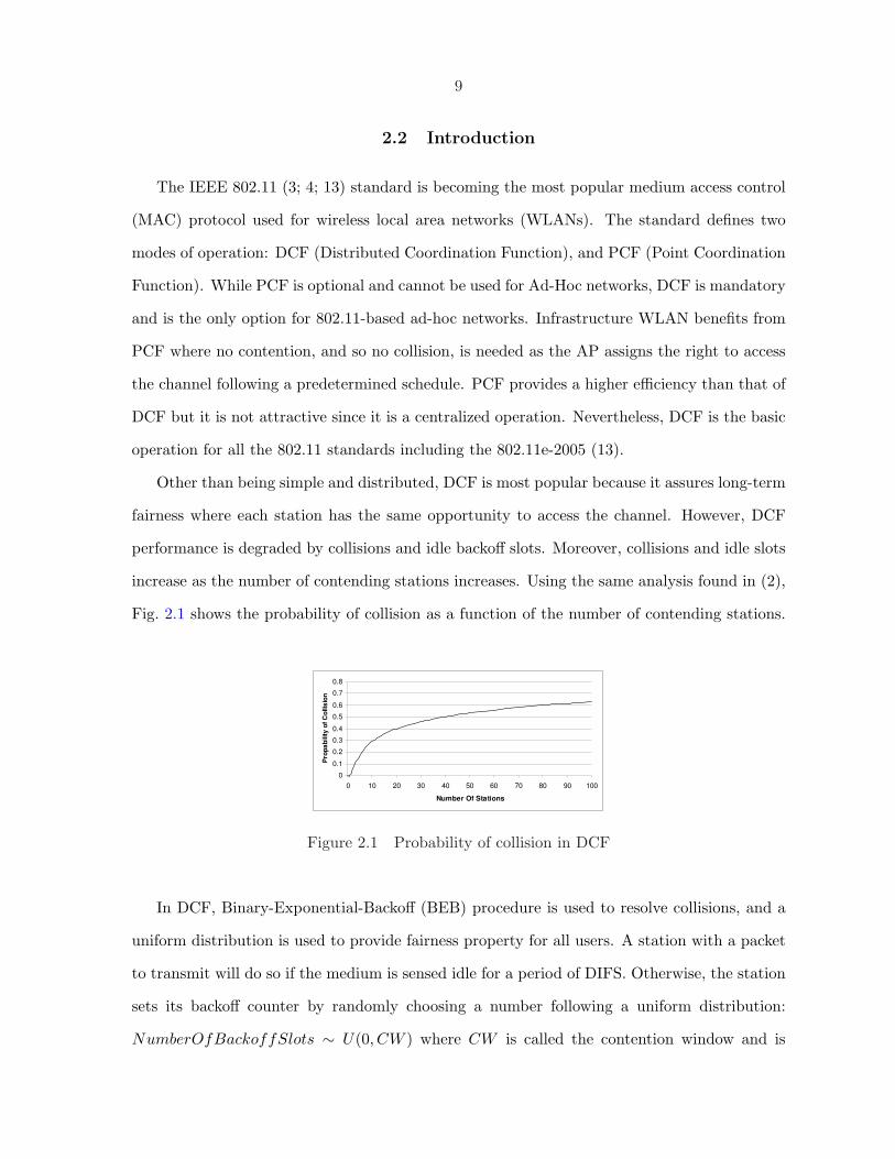
Other than being simple and distributed, DCF is most popular because it assures long-term
fairness where each station has the same opportunity to access the channel. However, DCF
performance is degraded by collisions and idle backoff slots. Moreover, collisions and idle slots
increase as the number of contending stations increases. Using the same analysis found in (2),
Fig. 2.1 shows the probability of collision as a function of the number of contending stations.
0
0.1
0.2
0.3
0.4
0.5
0.6
0.7
0.8
0 10 20 30 40 50 60 70 80 90 100
Number Of Stations
Pro
pa
bilit
y o
f C
ollis
ion
Figure 2.1 Probability of collision in DCF
In DCF, Binary-Exponential-Backoff (BEB) procedure is used to resolve collisions, and a
uniform distribution is used to provide fairness property for all users. A station with a packet
to transmit will do so if the medium is sensed idle for a period of DIFS. Otherwise, the station
sets its backoff counter by randomly choosing a number following a uniform distribution:
NumberOfBackoffSlots ∼ U(0, CW ) where CW is called the contention window and is

10
initially set to CWmin. The station decrements its backoff counter by one for every time slot
the medium is sensed idle, and transmits when this counter reaches zero. The destination
responds by sending an acknowledgment (ACK) back. The packets transmitted carry the time
needed to complete the transmission of a packet and its acknowledgement. This time is used by
all other stations to defer their access to the medium and is called Network Allocation Vector
(NAV). Collisions occur when two or more stations are transmitting at the same time. With
every collision, the station doubles its CW unless a maximum limit CWmax is reached, and
selects a new backoff counter from the new range. The process is repeated until the packet
is successfully transmitted or is dropped because a retry limit is reached. Unfortunately,
such behavior degrades the performance of the network especially under higher loads due to
collisions and idle slots. Even if the network has only one station transmitting, that station
still has to backoff for a number of slots. In addition, collisions occur more frequently when
the number of contending users increases. This results in an unstable behavior of DCF under
very high loads.
In this chapter, we propose a new contention management scheme named High-performance
DCF (HDCF), which addresses the problem of wasted time in contention resolution via clas-
sifying stations into active and inactive ones. Our objectives are to coordinate transmissions
from different active stations with no collisions or idle slots, and limit the contention to newly
transmitting stations. HDCF is a distributed random access scheme that achieves a higher
throughput while providing long-term and short-term fairness among all users. In general,
each station maintains a list of active users. The transmitting station chooses randomly the
next station to transmit from its own list of active users following a uniform distribution:
NextStationToTransmit ∼ U(first, last) where first and last are the first and last entries
of the active list. The selected station transmits after a PIFS period following the last trans-
mission, and other active stations will defer their attempts to transmit the same way NAV is
used in DCF. Thus, there are no collisions or redundant idle slots due to active transmissions.
On the other hand, a newly transmitting station uses an interrupt scheme. Thereafter, active
stations stop their active transmissions and only new stations would contend for the channel
11
using DCF. As a result, HDCF reduces the number of contending stations, and so collision
rates, and backoff slots. Results show that HDCF outperforms DCF in terms of throughput,
and fairness index with gains up to 391.2% and 26.8% respectively.
With HDCF, stations transmit in a uniform random order using a single channel with
no central control, no time synchronization, no slotted channel, and no periods’ reservations.
In addition, HDCF utilizes an interrupt scheme so that active stations (one or more) keep
transmitting unless there are new stations welling to transmit, and that those new stations
(one or more) can contend directly to assure fairness preventing unbounded delays for new
stations. Finally, HDCF works using the 802.11 PHY and MAC attributes (like NAV, retry
limits, fragmentation, and others), introduces no additional packets, and works with or without
RTS/CTS mode (e.g. used for hidden-terminal problem).
HDCF is presented in (59). In this chapter, we provide an analytical description of HDCF
compared to DCF. We use a simple but a well-known and an accurate model of the IEEE DCF
which is presented in (2). The analysis illustrates different issues of HDCF like fairness and
how collisions are reduced. In addition, the simulation experiments consider more results of
the IEEE 802.11b, VBR (variable rate traffic), and a mix of VBR and CBR (constant bit rate)
traffics.
The rest of this chapter is organized as following. Related work is summarized in section
2.3. In section 2.4, HDCF protocol’s details and rules are defined. In section 2.5, a simple
analytical analysis is provided to discuss performance and design issues of HDCF. In addition,
a simulation study is presented in section 2.6 to evaluate HDCF and compare it to DCF.
Finally, concluding remarks are given in section 2.7.
2.3 Related Work
To enhance DCF, many researchers proposed schemes that mainly attempt to reduce col-
lision rates, adapt CW to congestion levels, or find optimal values of CW . However, collisions
and wasted times still exist because some approaches solve one problem and leave another
(e.g., (5; 6; 7)), and optimal values are approximate and oscillate with the network conditions
12
that are variable (e.g., (5; 6; 7; 8; 9)). In addition, some schemes require the existence of an
access point (AP) or complex computations (e.g., (8; 9)). Instead of providing a history of all
such proposals, we will give examples that fall into these categories.
SD (5) divides CW by a factor after a successful transmission to improve fairness. FCR
(6) achieves a high throughput by having each station reset its CW to a minimal value after a
successful transmission, and double the CW exponentially after a collision or losing contention.
Thus, FCR requires the use of another mechanism to provide fairness. CONTI (7) attempts
to fix the total number of backoff slots to a constant value. Hence, there are always idle
slots and collisions may occur. In (8), the authors argued that the backoff value must be
set equal to the number of stations to maximize the throughput. This algorithm requires an
AP to broadcast the number of stations. Hybrid protocols (e.g. (9; 10)) divide the channel
into consecutive reserved contention and contention-free periods. Such protocols require a
central controller, reservation, multi-channels, the use of RTS/CTS, slotted channels, and/or
time synchronization. Also, new stations first wait for the contention-free periods to end
resulting in unbounded delays and unfairness especially when a new station waits more than
one contention-free period. Therefore, most of these schemes limit the number of active users
and lengths of different periods.
2.4 HDCF Details
HDCF utilizes an interrupt scheme and active transmissions to enhance fairness and elim-
inate, or reduce much of, the costs of contention of DCF (idle slots and collisions) without
adding any assumptions or constraints to DCF. The following subsections describe how HDCF
works.
2.4.1 Definitions
1. Active Stations and Active-List: active stations are those added to Active-List. Active-
List contains a list of stations that have more packets to transmit, hence the name Active
stations. Each station will maintain its own Active-List, and each entry of an Active-List
13
has the format < ID > where ID is the MAC address of an Active station. Active lists
may not be the same in all stations; active lists could be partial.
2. Next-Station: the station that is supposed to be the next transmitter and that is selected
by the currently transmitting station.
3. Active Transmissions: an active transmission is started by Next-Station after a PIFS
(PIFS = SLOT + SIFS) following the last transmission.
4. Idle Stations: stations that have no data to transmit.
5. New Stations: stations that were idle because they did not have data to transmit, and at
current time are having data to transmit. This includes mobile stations that move into
the network and have data to transmit, and stations that were turned off or in a sleep
mode and are turning on. New stations are also referred to as new arrivals.
2.4.2 Next-Station Selection
The current transmitting station, the source, will randomly select an entry from its Active-
List, and announce that ID as Next-Station. To provide fairness, a uniform distribution is
used:
Next-Station = Uniform(A[0], A[Size− 1]) (2.1)
where A[0] is the first entry and A[Size − 1] is the last entry of the station’s Active-List.
The announcing station does not have to be active. A transmitting station will make an
announcement even if it will not become active. This eliminates the need for active stations
to contend to get back into active mode.
Using the uniform distribution, an active station may choose itself as the next transmitter.
This assures the property provided by DCF which states that each station has the same
opportunity to access the channel. In addition, it prevents a station from wasting any idle
slots, no need to go through the backoff stages, if there are no other active stations.

14
MAC Header
Octets: 22 2 6 6 6 6 0 - 2312 4
Frame
Control
Duration
/ID
Sequence
ControlAddress 1 Address 3Address 2 Frame BodyAddress 4 FCS
Figure 2.2 MAC frame format
B0
Bits: 2
Protocol
VersionType Subtype
From
DS
To
DS
More
FragRetry
Pwr
Mgt
More
DataWEP Order
2 4 1 1 1 1 1 1 1 1
B1B2 B3 B4 B7 B8 B9 B10 B11 B12 B13 B14 B15
Figure 2.3 Frame Control field
2.4.3 Announcement
A station announces its future status by informing its neighbors, using broadcast nature
of wireless medium, that it does have or does not have more packets to transmit. In addition,
a station announces Next-Station; the next station that has the right to access the channel.
An announcement is performed by a station while it is transmitting. The advantage of this
behavior is that there is no need for any special frames or messages to be exchanged. Whenever
a station wins the right to access the channel, it will transmit a packet. The same packet can
be used for announcement.
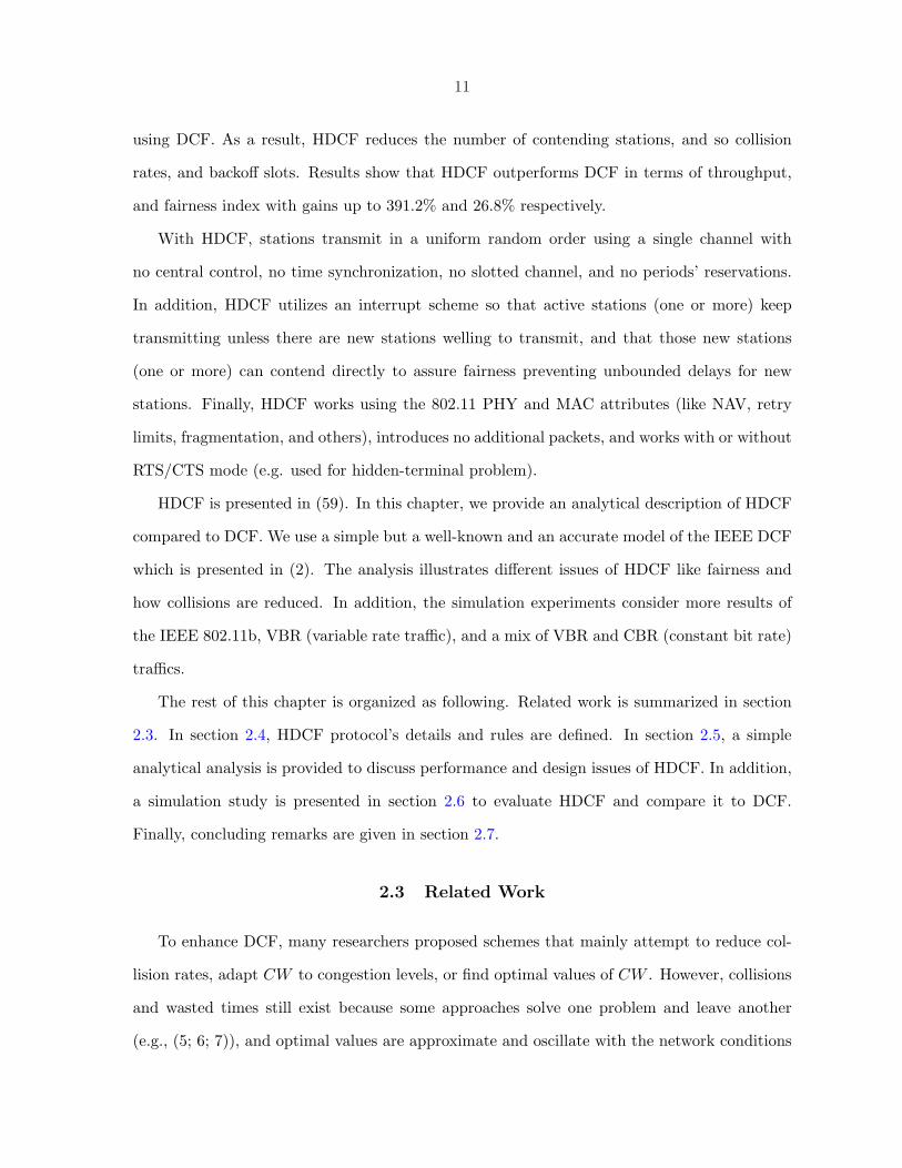
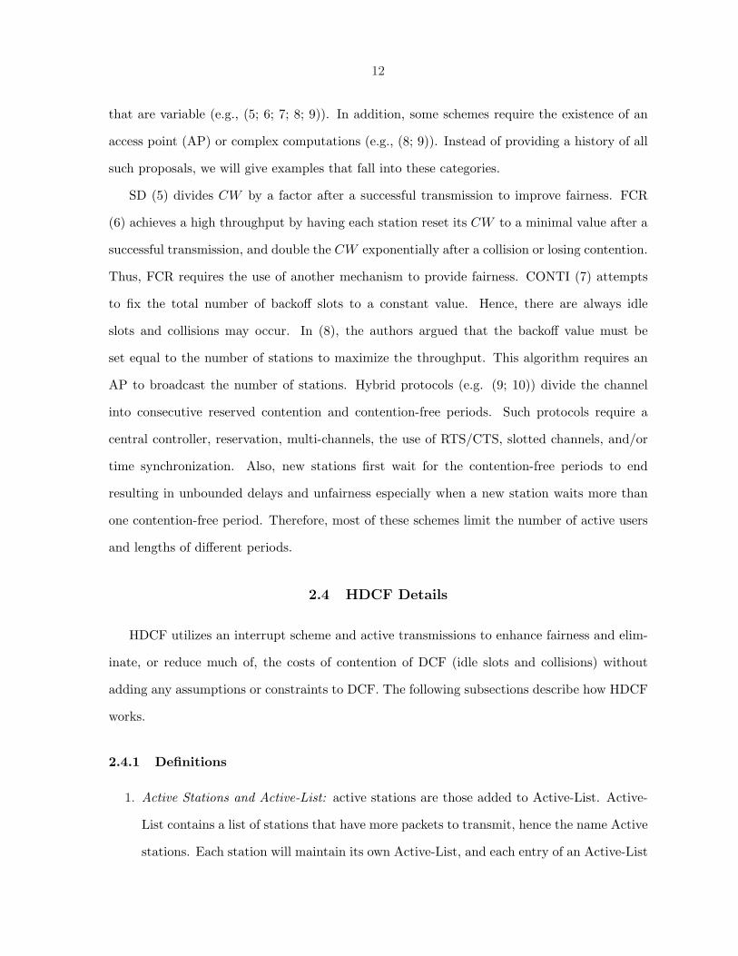
Using 802.11 packet formats, the ”More Data” bit of the Frame Control field, Fig. 2.3,
can be used for announcing that a station is active. The ”More Data” bit can be used since
it is used in PCF but not in DCF. Another bit called ”More Fragments” is used when more
fragments are to be transmitted with DCF. In addition, the header’s ”Address4” field of the
data frame, Fig. 2.2, can be used to announce Next-Station. This means an overhead of 6
bytes, the size of the MAC address which is small compared to the average packet size.
When a station receives, or overhears, a packet with the ”More Data” bit set to ”1”, it adds
an entry to its Active-List unless that entry already exists. The entry will be < ID >, where
ID is the MAC address of the transmitting node. On the other hand, if the ”More Data” bit
is set to ”0” then the entry, if exists, that has the MAC address of the transmitting node will
be removed from all overhearing stations’ Active-Lists. Note that for a station to be removed
from all Active-Lists, it needs to announce it only once; during the transmission of its last

15
packet.
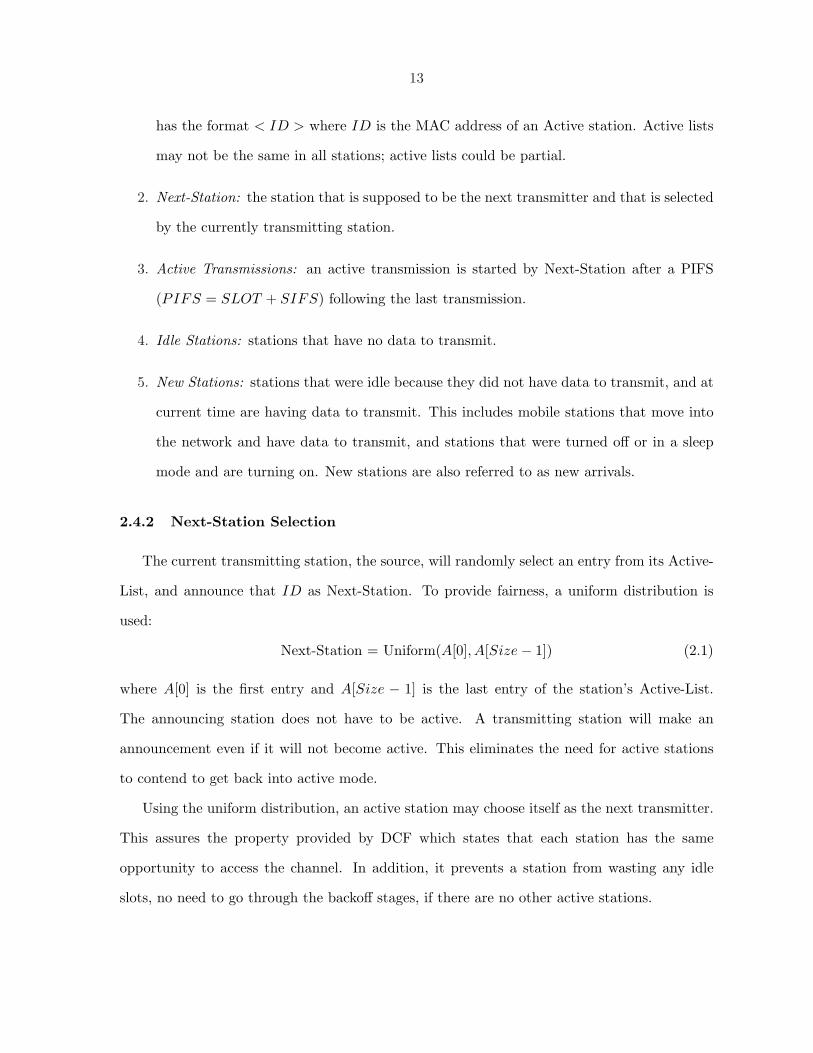
2.4.4 HDCF Rules
When a station wins the right to transmit, it will also announce Next-Station that is
selected randomly from its own Active-List. As shown in Fig. 2.4, active stations use PIFS as
an inter frame spacing (IFS): Next-Station starts transmitting PIFS after the end of the last
active station’s transmission. For the IFS between packets of the same transmission, SIFS is
used as in DCF. In addition, DCF NAV is still used, so stations will defer to the end of the
ongoing transmission.
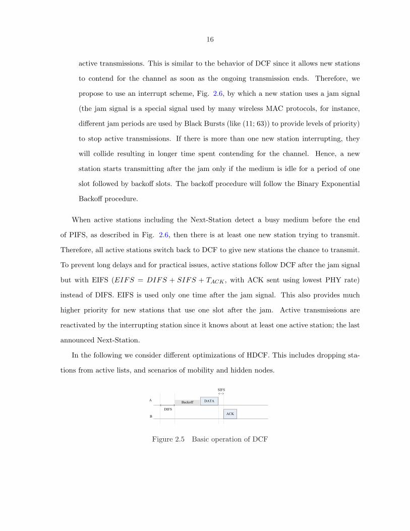
A new station initially assumes DCF; it transmits if the channel is idle for a period of DIFS
followed by backoff slots determined by Binary Exponential Backoff as shown in Fig. 2.5. If
there are active stations, then a new station will detect at least one active transmission since
PIFS is used as the IFS between any two consecutive active transmissions and PIFS is shorter
than DIFS. Therefore, following DCF rules would block a new station. There are two options
to allow a new station’s transmission:
1. Force active stations to switch back to DCF, or a silent mode, every while: every specific
limit of active transmissions or every time limit. Active stations need to wait only long
enough to check if there is any new station trying to transmit using DCF. A problem
with this approach is the overhead of time wasted when no new stations are arriving. In
addition, if there are more than two new stations, some of them may have to wait long
time before being able to start transmitting. This results in unfairness and unbounded
delays for new stations.
2. Allow a new station to interrupt active stations before the end of PIFS when they detect
Transmission 1 Transmission 2 Transmission 3PIFS PIFS
Data
ACK
SIFS
A
B
Figure 2.4 Active transmissions and their components
16
active transmissions. This is similar to the behavior of DCF since it allows new stations
to contend for the channel as soon as the ongoing transmission ends. Therefore, we
propose to use an interrupt scheme, Fig. 2.6, by which a new station uses a jam signal
(the jam signal is a special signal used by many wireless MAC protocols, for instance,
different jam periods are used by Black Bursts (like (11; 63)) to provide levels of priority)
to stop active transmissions. If there is more than one new station interrupting, they
will collide resulting in longer time spent contending for the channel. Hence, a new
station starts transmitting after the jam only if the medium is idle for a period of one
slot followed by backoff slots. The backoff procedure will follow the Binary Exponential
Backoff procedure.
When active stations including the Next-Station detect a busy medium before the end
of PIFS, as described in Fig. 2.6, then there is at least one new station trying to transmit.
Therefore, all active stations switch back to DCF to give new stations the chance to transmit.
To prevent long delays and for practical issues, active stations follow DCF after the jam signal
but with EIFS (EIFS = DIFS + SIFS + TACK , with ACK sent using lowest PHY rate)
instead of DIFS. EIFS is used only one time after the jam signal. This also provides much
higher priority for new stations that use one slot after the jam. Active transmissions are
reactivated by the interrupting station since it knows about at least one active station; the last
announced Next-Station.
In the following we consider different optimizations of HDCF. This includes dropping sta-
tions from active lists, and scenarios of mobility and hidden nodes.
ACK
DATAA
SIFS
Backoff
DIFS
B
Figure 2.5 Basic operation of DCF

17
Active
Transmission
The New Station
Interrupting
SIFS
JAMNew Station
Transmission
DIFS
Backoff Slots
SLOT
SLOT
Active
Transmission
PIFS
A New Station now has data to transmit
Figure 2.6 The interrupt scheme
2.4.4.1 Mobility
When considering mobility, HDCF may be optimized by allowing the drop of a station from
the local active list if it performs handover (or operations like disassociation), or if it does not
start transmitting for a number of times. A conservative value would be 1. However, a station
may not start an active transmission due to other reasons like those mentioned in subsection
2.4.6. Hence, we suggest the use of a higher value which also should not be very large - like 3.
2.4.4.2 Hidden Nodes
Like DCF, RTS-CTS operation should be used for the hidden terminal problem. Then
when a collision occurs due to the hidden terminal problem, all stations would switch back
to DCF and the collided transmitters would start backoff procedure. However, to enhance
the performance of HDCF when hidden nodes exist, we propose that the receiver rebroadcast
the next station address in the ACK frame. Accordingly, all stations within the ranges of the
receiver and the transmitter are aware of the address of the next station. Thereafter, a station
would defer accessing the channel if no activity is sensed for a period of RTS+SIFS when
the next station address is not within the active list. This would protect the transmission of a
hidden active station preventing a collision when the receiver is not hidden, i.e. waiting long
enough to hear the CTS frame.
Another improvement is to use ACK frames to rebroadcast the future status announce-
ment, i.e. having more data or not, of the transmitter. Thus, a node that is hidden (to the
transmitter) may add the transmitter to the active list. The address of the transmitter is
already included in the ACK frame. On the other hand, one control bit, in the ACK frame,
can be used to announce the future status, and is simply copied from the status announced in
18
the data frame. In addition, the ACK can be modified to re-announce the next station address.
Thus when selected by a hidden transmitter, a station can be selected to be the transmitter.
Finally, HDCF stations may adapt their transmissions according to network and channel
characteristics using different techniques used for the 802.11 DCF like the use of RTS/CTS
operation for hidden nodes, RTS threshold, and fragmentation.
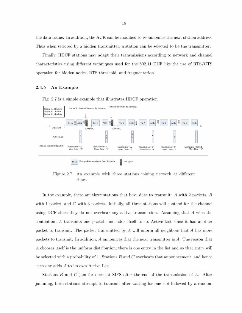
2.4.5 An Example
Fig. 2.7 is a simple example that illustrates HDCF operation.
Tx_A ACK
Station B, Station C interrupt by jamming
Tx_C
A
ACK
A
C
Tx_B ACK
A
C
Station B interrupts by jamming
Tx_A ACK
C
NextStation = A NextStation = A NextStation = A NextStation = C
Tx_C ACK
C
NextStation = C
SLOT+BO
SIFS
SIFS
SLOT+BODIFS+BO
Station A, 2 Packets
Station B, 1 Packet
Station C, 3 Packets
PIFS
PIFS
SIFS
More Data = ‘1' More Data = ‘1' More Data = ‘0' More Data = ‘0' More Data = ‘1'
Tx_C ACK
PIFS
Tx_A Data packet transmission from Station A Jam signal
Active-List:
Info. on transmitted packet:
More Data = ‘0'NextStation = NONE
Figure 2.7 An example with three stations joining network at differenttimes
In the example, there are three stations that have data to transmit: A with 2 packets, B
with 1 packet, and C with 3 packets. Initially, all three stations will contend for the channel
using DCF since they do not overhear any active transmission. Assuming that A wins the
contention, A transmits one packet, and adds itself to its Active-List since it has another
packet to transmit. The packet transmitted by A will inform all neighbors that A has more
packets to transmit. In addition, A announces that the next transmitter is A. The reason that
A chooses itself is the uniform distribution; there is one entry in the list and so that entry will
be selected with a probability of 1. Stations B and C overhears that announcement, and hence
each one adds A to its own Active-List.
Stations B and C jam for one slot SIFS after the end of the transmission of A. After
jamming, both stations attempt to transmit after waiting for one slot followed by a random

19
number of backoff slots. Assume that C wins the contention. C adds itself to its Active-List,
and transmits while announcing A as the next transmitter, assuming that A was selected. The
active list is updated at each of the three stations to include both: A, and C. Station B jams
the channel for one slot SIFS following the transmission of C, then it transmits after a period
of one slot and a number of backoff slots. Note that station B announces that it has no more
data to transmit. Now the active list at each station includes stations A and C. Moreover, B
announces A as the next transmitter, and so A transmits PIFS after transmission of B as no
more stations are interrupting.
Node A transmits while announcing that it has no more data to transmit and that C is
the next transmitter. As a result, Active-Lists at all stations are updated to include only
C. Station C transmits PIFS after the transmission of A while announcing itself as the next
transmitter, and that it has more data to transmit. Station C transmits its last packet without
any interrupt announcing no more data to transmit. All three stations update there Active-lists
that become empty.
2.4.6 Recovery Mechanism
Because of hidden terminal problem, channel errors, mobility, and the sudden shut down
(turning power off) of any station, it is possible that the next selected station would not be
able to start its transmission. In such case, all other active stations would notice the absence
of Next-Stations’s transmission just after a PIFS period by SIFS. Therefore, active stations
are required to temporarily contend for the channel using DCF as a recovery mechanism, see
figure 2.8 for the timings of switching to DCF (note there is no overhead to original timing in
DCF since DIFS = PIFS + SIFS). Once active transmissions are recovered, active stations
will switch back to the active state.
No transmission seen from
Next-Station
SIFSPIFS
Transmission 1 Defer Backoff
Figure 2.8 Recovery from a lost announcement

20
Moreover, different scenarios may arise because of wireless channel conditions. One scenario
may occur when an active station, other than the next selected one, can overhear but cannot
decode a packet that carries an announcement. This active station should temporaliy switch
back to DCF operations. As a result, the announced next station would start transmitting
with no problems, if it does hear the announcement. Another situation is when an active
transmitter does not receive an ACK. This would be seen as a collision by this transmitter.
Moreover, a station may handover and later is selected as the next transmitter. Hence, that
station may not be able to start an active transmission. In summary, recovery is achieved by
having active stations switch back to DCF operations and active stations will re-follow HDCF
rules as soon as Next-Station is announced.
2.4.7 Summary, and Advantages
An HDCF station operates in one of two modes: active mode, and contending mode.
In active mode, there are no backoff, no collisions, and no idle slots. On the other hand,
contending mode uses legend DCF but with much lower collision rate because almost only
new stations contend for the channel. The way Next-Station is selected, and the interrupt
scheme have different advantages: 1) No idle slots wasted when there are no new stations;
i.e. no need to stop active transmissions. 2) Fairness to new stations as they can contend for
the channel directly (like in DCF) without long delays as contention cost is much smaller. 3)
Stations transmit in random order without the need for slotted channel, reserved periods, time
synchronization, central control, or knowledge of number of active users.
Finally, Just like 802.11 DCF, HDCF stations may adapt their transmissions according to
network and channel characteristics using different techniques used for the 802.11 like RTS
threshold, fragmentation, link adaptation, and the use of RTS/CTS for hidden nodes.
2.5 Performance Analysis
In this section, excluding subsection 2.5.5, the same assumptions and the analysis model
described in (2) are used for simplicity in analysis and discussion. There are n stations with

21
each station always has a packet to transmit. In addition, all stations can overhear each other
transmission, i.e., there are no hidden terminals. A DCF network of greedy stations is modeled
using a nonlinear system of equations that can be solved by means of numerical techniques.
To summarize the analysis model, let τ be the probability that a station transmits in any slot
time. The value τ can be found by solving the following non-linear system:
τ =2(1− 2ρ)
(1− 2ρ)(W + 1) + Wρ(1− (2ρ)m))(2.2)
ρ = 1− (1− τ)n−1 (2.3)
Where ρ is the probability that the transmitted packet will collide. W is equivalent to CWmin,
and m is the maximum backoff stage where CWmax = 2mCWmin. Moreover, let Ptr be
the probability of transmission, Ps the probability of a successful transmission, and Pc the
probability of collision.
Ptr = 1− (1− τ)n (2.4)
Ps =nτ(1− τ)n−1
1− (1− τ)n(2.5)
Pc = 1− Ps (2.6)
Pidle = 1− Ptr (2.7)
Then, the expected number of idle slots can be calculated by:
E[Number of idle slots] =1
Ptr− 1 (2.8)
The following subsections discuss special performance issues in HDCF compared to other
schemes.
2.5.1 How to Handle New Arrivals
For DCF, if x more stations become ready to transmit, then there is a need only to replace n
by n+x. The reason is that, under DCF all stations are contending for the channel with equal
opportunities. For HDCF, the situation is different since only the new stations will contend
for the channel. Starting with n active stations, the transmission probability is 1 and collision

22
Timet1t0 t2
Number of
Contending
Stattions
n
n+x
0
x
0
x-1
…..
…………...
.…1
Number of
Contending
Stattions
HDCF
Time
DCF
Network Size
= n stations
Network Size
= (n+x) stations
….
n n-1 1
0
0
Figure 2.9 New arrivals effect on contention level
probability is 0. If x new stations become ready to transmit, then equations (2.2) and (2.3)
can be used by replacing n with x. Only the new x stations will be contending for the channel.
Once a new station becomes active, the contention is reduced to be among x−1 stations. This
is repeated until all x stations become active, and therefore, the collision goes back to zero. In
other words, stations go back into active mode after being in contending mode.
Fig. 2.9 explains this behavior for both DCF and HDCF. The network size from 0 to t1 is
n, and n + x after t1. For DCF, all existing stations contend for the channel. On the other
hand, the number of contending stations is variable for HDCF case. At t = 0, n stations start
contending for the channel. Once a station becomes active, it will not contend for the channel.
Hence, number of contending stations drops by one after every successful transmission until all
nodes become active at t0. There is no contention from t0 to t1 since all n stations are active.
However, x new arrivals occur at t1 and all of them will become active. Hence, contention from
t1 to t2 is only among the new x arrivals. Once a station successfully transmits and joins the
active list, it will no longer contend for the channel using DCF rules. This is repeated until all
x stations become active, and therefore, no more contention occurs. The next winner of the
channel will be determined by the transmitting station using the uniform random distribution
described in section 2.4. Fig. 2.10 shows a comparison between the probability of collision of
DCF and HDCF. The x-axis in the figure shows steps of collision resolution, and the y-axis
is the probability of collision. The comparison is made for a system that starts with 5 active
stations. After some time, 10 new stations are added to system. Under DCF, the probability
of collision increases to that of 15 contending stations. The probability of collision stays at

23
Propability of Collision (p)
0
0.1
0.2
0.3
0.4
0.5
1 2 3 4 5 6 7 8 9 10 11 12
Time
p
HDCF
DCF
Figure 2.10 Probability of collision comparison
that level. On the other hand, HDCF starts with a probably of collision of 10 stations. After
that, the probability drops to that of 9 stations. The process is repeated until all stations are
active, and the probability of collision becomes 0.
To understand the importance of reducing collision probability, the expected number of
backoff slots a station will experience per packet can be expressed:
Wbackoff = (1− ρ)20W
2+ ρ (1− ρ)
21W
2
+........ + ρm(1− ρ)2mW
2
= (1− ρ− ρ(2ρ)m
1− 2ρ)(
W
2) (2.9)
Again, ρ is the probability that a packet transmitted will collide, W is CWmin, and m is
the maximum backoff stage. Hence, the number of backoff slots increases when more stations
are contending for the channel. HDCF mitigates the problem during contention by reducing
number of contending stations linearly with every successful transmission. The result would
be increasing the throughput and reducing the delay seen by different stations.
2.5.2 How Contentions Are Resolved
Compared to DCF, HDCF is designed to achieve a higher performance while maintaining
an important feature provided by DCF. In DCF, every station has equal opportunity to access
the channel. This results in throughput-based fairness property. DCF operation consists of
cycles such that on average, each cycle includes a transmission by each user in the network.
Using the results of (2), it can be proved that such a cycle is reached by stations. Let n be
the number of active stations in the network and υ be the probability that a given station
transmits successfully for the next slot following DCF rules. Also, let X be the number of

24
stations transmitting between two consecutive transmissions of a given station. The random
variable X follows a geometric distribution:
υ =τ(1− τ)n−1
nτ(1− τ)n−1=
1n
(2.10)
P [X = k] = υ(1− υ)k =1n
(1− 1n
)k (2.11)
E[X] =1v− 1 = n− 1 (2.12)
The E[X] value implies that on average each station transmits once in a cycle consisting of
transmissions from all stattions. On the other hand, using HDCF, it can also be proved that
a cycle exits such that every station takes turn to transmit. Now, let υ be the probability
that a given station transmits following HDCF rules. The random variable X also follows a
geometric distribution:
υ =1n
(2.13)
P [X = k] = υ(1− υ)k =1n
(1− 1n
)k (2.14)
E[X] =11n
− 1 = n− 1 (2.15)
The difference between HDCF and DCF is that DCF achieves this property with the cost
of idle slots and collisions. On the other hand, HDCF is free of such overheads, and thus is
expected to enhance the fairness property (verified by simulation results, section 2.6). In DCF,
equation (2.10) is equivalent to the probability that a station successfully transmits while all
others do not, and equation (2.11) accounts for a variable number of collided and idle slots
before such a transmission occurs. However, equation (2.13) of HDCF is equivalent to the
probability that a station successfully transmits after being selected using a random uniform
distribution with n distinct outputs, and equation (2.14) accounts for a variable number of
successful transmissions before such a transmission occurs.
Throughput-based fairness is proper for a single-rate network. However, in a multi-rate
wireless network where users have different rates, throughput-based fairness degrades the over-
all network performance and the higher rate stations performance. The reason is that stations
with slower rates occupy the channel for longer times. In such an environment, time-based

25
fairness is desired. Time-based fairness allocates same amount of resources, time, to all users
regardless of their data rates. The same techniques used in a DCF network to achieve time-
based fairness can also be used for HDCF. For example, in OAR mechanism (62), a station
may transmit a number of packets in proportion to its data rate once it wins the contention.
2.5.3 Maximum Achieved Throughput
The maximum saturation throughput of a DCF network can be approximated by:
SDCF =E[L]
DIFS + SIFS + CWmin2 σ + Tack + Tdata
(2.16)
Here, σ is one slot time, Tdata is the time needed to send one data packet, Tack is the time
needed to send an ACK, and E[L] is the average packet size.
On the other hand, we can approximate the maximum saturation throughput that can be
achieved using HDCF:
SHDCF =E[L]
PIFS + SIFS + Tdata + Tack(2.17)
Note that the time needed by stations to join the active mode is ignored. Using these formulas,
one can expect a high gain by using HDCF. The simulation results, section 2.6, show that
HDCF outperforms DCF and provides an efficient performance.
2.5.4 Packets Transmission Differences
This section explains the differences in how packets are transmitted in different schemes
compared to HDCF. Fig. 2.11(a) explains the operation of DCF with burst mode. A station
is allowed to transmit more than one packet after winning a contention using DCF rules. The
contention period includes DIFS and backoff timer. Fig. 2.11(c) shows the operation of PCF,
a polling-based scheme which requires the existence of a PC (Point Coordinator) which usually
is at the AP. The PC assigns the right of accessing the channel to different stations by the use
of polling messages. In general, PCF is not an attractive method because it is centralized and
it introduces the overhead of polling. Refer to (3) and (64) for more information about polling
schemes. Finally, Fig. 2.11(b) shows packets transmission in HDCF. Notice that it is fairer

26
compared to other schemes in Fig. 2.11, and at same time has no collisions or idle slots when
stations are all active.
Data 1 ACK Data 1 ACK Data 2 ACK …..Contention period
SIFS SIFS SIFS SIFS
Contention
period
(a) DCF burst mode
Data 1 ACK Data 3 ACK Data 1 ACK …..Data 2 ACK
SIFS SIFSSIFS SIFSPIFS PIFS PIFS
(b) HDCF
Poll 1 Data+Poll 2 ACk Poll 3 Data ACK ….. ENDBeacon
SIFS PIFS SIFSSIFS SIFS SIFS
(c) PCF
Figure 2.11 Different modes of transmissions
2.5.5 Approximate Analysis
Now we provide an approximate analysis for the system at a given state. Assume a Poisson
arrival process with λ packets per second at each station. Consider the system’s state where
there are m active stations, and n −m stations are not active. Let γ be the probability that
a station has a packet at the end of the last active transmission, and X be a random variable
that represents the number of stations that would jam after the last active transmission. The
probability γ is equivalent to the probability that at a given station, there was at least one
arrival during the service time of an active transmission Ta (PIFS + SIFS + Tdata + Tack). If
N is a random variable representing the number of packets at a station after Ta, then:
γ = P [N(Ta) ≥ 1]
= 1− P [N(Ta) = 0]
= 1− e−λTa (2.18)
P [X = x] =(
n−m
x
)γx(1− γ)n−m−x (2.19)
E[X] = (n−m)γ (2.20)
Hence, the throughput can be approximated by:
SHDCF |m =(1 + E[X])LTa + 1
µE[X]
(2.21)

27
Here, µE[X] is the service rate of DCF given that there are E[X] stations with data to
transmit, and L is the packet size. Equation (2.21) converges to (2.17) when there are no
interrupting stations, and to (2.16) when some or all stations always contend for the channel
but with one packet per station at each time.
2.6 Simulation
This section presents the simulation we used to evaluate the performance of HDCF and
compare it to that of the IEEE 802.11 DCF. We utilized the commercial Opnet Modeler 11.5.A,
(1), to implement HDCF by modifying the 802.11 model.
The simulations are performed for networks using two different PHYs, 802.11b and 802.11g.
Table 2.1 shows the parameters used by the Opnet 802.11 model. We consider different
scenarios to study the performance of HDCF and compare it to that of DCF. First, we assume
a fully-connected network with no channel errors; collisions are the only source of errors.
Here, we start with a saturated scenario to provide a reference and an understanding of the
maximum achievable performance. Second, we study the performance under different loads, or
a non-saturated network. We also consider CBR (Constant Bit Rate) and VBR (Variable Bit
Rate) traffic sources. Finally, we study the performance under different noise levels (channel
conditions). To implement noise, we used a jammer node provided by Opnet.
2.6.1 Performance Metrics
For performance measurements, we use the following metrics:
1) Throughput: the total data transmitted per the simulation period. The simulation consid-
ered the throughput versus different sizes of packets, different number of stations, and different
offered loads. We used normalized throughput defined as Throuput/RateMAC .
2) Fairness Index: we used Jain Index, (12; 65), defined by (2.22):
JF =(∑n
i=1 Si)2
n∑n
i=1 S2i
(2.22)
Where n is number of stations and Si is the throughput of station i. The closer the value of
FI to 1, the better the fairness provided. We provide results for different simulation periods

28
Table 2.1 Network Parameters
Parameter 802.11g 802.11b Parameter 802.11g 802.11b
aSlotT ime 20µs 20µs SIFS 10µs 10µs
PIFS 30µs 30µs DIFS 50µs 50µs
CWmin 15 31 CWmax 1023 1023
PLCP Overhead 20µs 192µs DCF Overhead 28 Bytes 28 Bytes
MAC ACK Size 14 Bytes 14 Bytes HDCF Overhead 34 Bytes 34 Bytes
Data Rate 54Mbps 11Mbps ControlRate 24Mbps 1Mbps
to have better conclusions about both long and short term fairnesses.
2.6.2 Saturated Stations
This section provides a comparison between DCF and HDCF for a network of fully con-
nected and saturated stations, i.e stations that have data packets to transmit at all times.
Fig. 2.12 compares the normalized throughput between HDCF and DCF for 50 contending
stations as a function of the packet size, which changes from 50 bytes to 2304 bytes. For
HDCF, the normalized throughput reaches values of about 72.7% for 802.11b and 74.4% for
802.11g networks. For DCF, the values are about 48% and 33.8% for 802.11b and 802.11g
networks respectively. The gain goes from 45.7% to 64% for 802.11b, and from 119.8% to
282.5% for 802.11g. One can see that the normalized throughput increases with the packet
size for both protocols. However, the gain increases as the packet size gets smaller. This is due
to the fact that collision’s cost is higher as it takes longer time for larger packets. In addition,
the figure shows the maximum normalized throughput values estimated by equations (2.17)
for HDCF and (2.16) for DCF. While HDCF almost achieves the maximum performance, DCF
performance is always lower than the maximum possible values.
Fig. 2.13 compares the normalized throughput between HDCF and DCF as a function of
the network size, number of stations. Here, the packet size is fixed at 1000 bytes. Fig. 2.13
shows a higher stability performance of HDCF; the number of stations has small effect on
the performance of HDCF. On the other hand, DCF performance degrades as the number of

29
0
10
20
30
40
50
60
70
80
90
0 500 1000 1500 2000 2500
Packet Size (Bytes)
No
rmali
zed
Th
rou
gh
pu
t (%
)
DCF - 802.11b HDCF - 802.11b
DCF - 802.11g HDCF - 802.11g
MAX - DCF 802.11b MAX - HDCF 802.11b
MAX - HDCF 802.11g MAX - DCF 802.11g
Figure 2.12 Throughput vs. packet size
stations gets larger. The main reason is that, the probability of collisions in DCF increases
exponentially when number of stations increases. Moreover, all stations contend for the channel
all times. However, HDCF reduces the number of contending stations linearly, and remove any
unnecessary idle slots. Hence, collision probability and overheads are much reduced by HDCF
allowing a higher stability.
0
10
20
30
40
50
60
70
0 20 40 60 80 100 120
Number of stations
No
rma
lize
d T
hro
ug
hp
ut
(%)
DCF - 802.11b HDCF- 802.11b DCF - 802.11g HDCF- 802.11g
Figure 2.13 Throughput vs. network size
In Fig 2.14, we summarize results from different simulations we conducted. The figure
shows the minimum and maximum gains of normalized throughput for different network sizes.
Again, packet size is changed from 50 to 2304 bytes for each simulation. The least gain is
10.5%, and the greatest is 391.2%. In all cases, the gain increases when the number of stations
increases.
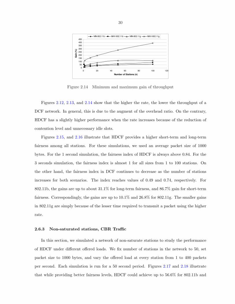
30
0
50
100
150
200
250
300
350
400
450
0 20 40 60 80 100 120
Number of Stations (n)G
ain
(%
)
MIN-802.11b MAX-802.11b MIN-802.11g MAX-802.11g
Figure 2.14 Minimum and maximum gain of throughput
Figures 2.12, 2.13, and 2.14 show that the higher the rate, the lower the throughput of a
DCF network. In general, this is due to the augment of the overhead ratio. On the contrary,
HDCF has a slightly higher performance when the rate increases because of the reduction of
contention level and unnecessary idle slots.
Figures 2.15, and 2.16 illustrate that HDCF provides a higher short-term and long-term
fairness among all stations. For these simulations, we used an average packet size of 1000
bytes. For the 1 second simulation, the fairness index of HDCF is always above 0.84. For the
3 seconds simulation, the fairness index is almost 1 for all sizes from 1 to 100 stations. On
the other hand, the fairness index in DCF continues to decrease as the number of stations
increases for both scenarios. The index reaches values of 0.49 and 0.74, respectively. For
802.11b, the gains are up to about 31.1% for long-term fairness, and 86.7% gain for short-term
fairness. Correspondingly, the gains are up to 10.1% and 26.8% for 802.11g. The smaller gains
in 802.11g are simply because of the lesser time required to transmit a packet using the higher
rate.
2.6.3 Non-saturated stations, CBR Traffic
In this section, we simulated a network of non-saturate stations to study the performance
of HDCF under different offered loads. We fix number of stations in the network to 50, set
packet size to 1000 bytes, and vary the offered load at every station from 1 to 400 packets
per second. Each simulation is run for a 50 second period. Figures 2.17 and 2.18 illustrate
that while providing better fairness levels, HDCF could achieve up to 56.6% for 802.11b and

31
0
0.2
0.4
0.6
0.8
1
1.2
0 20 40 60 80 100 120
Number of Stations
Fair
ness I
nd
ex (
%)
DCF 802.11b
HDCF 802.11b
DCF 802.11g
HDCF 802.11g
Figure 2.15 Fairness Index for 1 second period
0
0.2
0.4
0.6
0.8
1
1.2
0 20 40 60 80 100 120
Number of Stations
Fair
ness I
nd
ex (
%)
DCF 802.11b
HDCF 802.11b
DCF 802.11g
HDCF 802.11g
Figure 2.16 Fairness Index for 3 seconds period
168.3% for 802.11g more throughput than that of DCF.
From the previous experiments, we select a load rate of 20 packets per second and vary
network size from 1 to 100 stations. Figures 2.19 and 2.20 show that HDCF concurrently
improves fairness and provides throughput gains as high as 81.8% and 71.7% for the 802.11b
and 802.11g networks respectively.
Figures 2.17 and 2.18, 2.19, and 2.20 also explain that once the network load, or the
network size, gets beyond a certain level, DCF performance starts to degrade due to higher
contention levels. Alternatively, HDCF enhances the performance because it reduces number
of contending stations and unnecessary idle slots. In addition, HDCF performs just like DCF
when the network load is light or when the network size is small. In such cases, DCF is proved
to be highly efficient. Consequently, HDCF achieves higher performance and adapts better to
different loads and network sizes.

32
0
10
20
30
40
50
60
0 100 200 300 400 500Number of packets per node per second
No
rmali
zed
Th
rou
gh
pu
t
(%)
0.982
0.984
0.986
0.988
0.99
0.992
0.994
0.996
0.998
1
1.002
Fair
ness I
nd
ex
Throughput - DCF Throughput - HDCF JF - DCF JF - HDCF
Figure 2.17 Throughput vs. load, 802.11b
0
10
20
30
40
50
60
70
0 100 200 300 400 500
Number of packets per node per second
No
rmalized
Th
rou
gh
pu
t
(%)
0.995
0.996
0.997
0.998
0.999
1
1.001
Fair
ness In
dex
Throughput - DCF Throughput - HDCF JF - DCF JF - HDCF
Figure 2.18 Throughput vs. load, 802.11g
0
10
20
30
40
50
60
0 20 40 60 80 100 120
Number of stations
No
rma
lize
d T
hro
ug
hp
ut
(%)
0.98
0.985
0.99
0.995
1
1.005
Fa
irn
es
s In
de
x (
JF
)
Throughput - DCF Throughput - HDCF JF - DCF JF - HDCF
Figure 2.19 Throughput vs. number of users, 802.11b

33
0
5
10
15
20
25
30
35
0 20 40 60 80 100 120
Number of stations
No
rmalized
Th
rou
gh
pu
t (%
)
0.994
0.995
0.996
0.997
0.998
0.999
1
1.001
Fair
ness In
dex (
JF
)
Throughput - DCF Throughput - HDCF JF - DCF JF - HDCF
Figure 2.20 Throughput vs. number of users, 802.11g
0
0.2
0.4
0.6
0.8
1
1.2
0 10 20 30 40 50 60
Time (Seconds)
Fair
ness In
dex (
JF
)
0
10
20
30
40
50
60
70
80
Gain
(%
)DCF - 802.11b
HDCF - 802.11b
DCF - 802.11g
HDCF - 802.11g
Gain - 802.11b
Gain - 802.11g
Figure 2.21 Fairness Index vs. time
Finally, we provide results for different simulation’s periods to have better conclusions
about short-term fairness. Fig. 2.21 presents fairness index vs. duration for a network of 80
stations, and a constant packet interarrival time of 0.01 second at each station. The gains
can reach values up to 70.6% and 23.6% for 802.11b and 802.11g respectively. Since the gain
increases for shorter periods, HDCF improves the short-term fairness of the network. Such
enhancement is related to throughput’s improvements as explained above, and how the next
station is selected (see section 2.4.2).
2.6.4 Non-saturated stations, VBR Traffic
Here, we consider a network of 50 users, and 500 bytes per packet. Simulation period is
50 seconds. Instead of using CBR traffic, packets are generated at each user following the
distribution Exponential(λ), where λ is the mean interrival time (in seconds). Since packets’

34
generation does not follow a CBR distribution, different users may have different loads. Hence,
we redefine JF:
JF =(∑n
i=1SiLi
)2
n∑n
i=1(SiLi
)2(2.23)
where Li is the total normalized load of user i.
Figures 2.22 and 2.23 show the throughput and fairness index as a function of λ. It
is clear that HDCF provides always the same or better fairness levels. In addition, HDCF
outperforms DCF when considering the total throughput with gains up to 58.7% (169.7%)
for 802.11b (802.11g). The figure explains that beyond some threshold of normalized load
(about 22.7% (9.2%) at λ = 80m (40m) second for 802.11b (802.11g)), HDCF adapts better
to different loads at different users and therefore enhances the performance of the network.
0
5
10
15
20
25
30
35
40
45
0 20 40 60 80 100 120
Interarrival Time (x10-3 seconds)
No
rmali
zed
Th
rou
gh
pu
t (%
)
0.99
0.992
0.994
0.996
0.998
1
1.002
Fair
ness I
nd
ex
Throughput-DCF Throughput-HDCF JF-DCF JF-HDCF
Figure 2.22 Network with VBR traffic, 802.11b
0
5
10
15
20
25
30
35
40
0 20 40 60 80 100 120
Interrival Time (x10-3 seconds)
No
rmali
zed
Th
rou
gh
pu
t (%
)
0.996
0.9965
0.997
0.9975
0.998
0.9985
0.999
0.9995
1
1.0005
Fair
ness I
nd
ex
Throughput-DCF Throughput-HDCF JF-DCF JF-HDCF
Figure 2.23 Network with VBR traffic, 802.11g

35
Finally, we modify network configuration so that 10 users generate CBR traffic with 40m
seconds interrival time, and 40 users generate VBR traffic as described above. Figures 2.24
and 2.25 show that while providing slightly a higher fairness level, HDCF achieves higher
throughput with gains up to about 57.5% (130.3%) for 802.11b (802.11g). Again, HDCF
adapts better to different users’ loads.
0
5
10
15
20
25
30
35
40
45
0 20 40 60 80 100 120
Interarrival Time (x10-3 seconds)
No
rmali
zed
Th
rou
gh
pu
t (%
)
0.5
0.6
0.7
0.8
0.9
1
1.1
Fair
ness I
nd
ex
Throughput-DCF Throughput-HDCF JF-DCF JF-HDCF
Figure 2.24 Network with both CBR and VBR traffic, 802.11b
0
5
10
15
20
25
30
35
0 20 40 60 80 100 120
Interrival Time (x10-3 seconds)
No
rmali
zed
Th
rou
gh
pu
t (%
)
0.82
0.84
0.86
0.88
0.9
0.92
0.94
0.96
0.98
1
1.02F
air
ness I
nd
ex
Throughput-DCF Throughput-HDCF JF-DCF JF-HDCF
Figure 2.25 Network with both CBR and VBR traffic, 802.11g
As illustrated in CBR scenarios, HDCF performs just like DCF when the network load is
light where DCF is proved to be highly efficient. However, HDCF outperforms DCF under
higher loads. In other words, HDCF achieves higher performance and adapts better to different
loads and network sizes.

36
2.6.5 Channel Noise
The results provided are for a network of 50 stations with CBR traffic of 50 packets per
second. Each packet is 1000 bytes, and each simulation is run for 100 seconds. To implement
noise, we used a jammer node provided by Opnet. The jammer was configured to produce
noise signals with a constant length of 1024 bits/signal at a constant rate varied for different
runs. Fig. 2.26 shows the performance measures vs. the number of noise bits per second for an
802.11g network. In this figure, the x-axis is log-scaled. The figure show that the throughput
gain increases up to about 93.7%, and then starts to decrease until there is no gain when the
channel errors are very high. Furthermore, HDCF provides higher throughput and fairness for
all tested noise levels.
For both protocols, stations defer their access to the channel whenever sensed busy. How-
ever, the number of contending stations would increase when more noise is introduced. As a
result, the performance of DCF degrades since more stations are contending; a higher collision
rate and backoff slots. Quite the opposite, HDCF would reduce number of contending stations
and unnecessary idle slots. Moreover, active stations would always recover from channel errors
as explained in section 2.4.6. Thus, HDCF performance is steady as long as errors are not
severe. Once the noise reaches a very high level, both protocols are severely affected.
0
5
10
15
20
25
30
35
40
1000 10000 100000 1000000
Noise bits per second
No
rma
lize
d T
hro
ug
hp
ut
(%)
0.995
0.996
0.997
0.998
0.999
1
1.001
Fa
irn
es
s In
de
x (
JF
)
Throughput - DCF Throughput - HDCF
JF - DCF JF - HDCF
Figure 2.26 Throughput vs. noise level, 802.11g

37
2.7 Conclusions
In IEEE 802.11 wireless networks, DCF is the basic channel access scheme. However, the
performance of DCF degrades when the network size (number of users) or offered loads get
larger because of higher contention levels, and so more idle slots and higher collision rates. In
this chapter, we proposed a new high-performance DCF (HDCF) MAC protocol to address
the problem of wasted time in contention resolution in DCF. HDCF eliminates the need for
unnecessary contention and idle slots by allowing transmitting stations to select the next user to
transmit. To assure fairness, next station is selected in a random uniform fashion. In addition,
new stations utilize an interrupt scheme to contend directly without delays. Thereafter, active
stations would stop their active transmissions and only new stations would compete for the
channel using DCF. As a result, HDCF reduces the number of contending stations, and so
collision rates, and backoff slots. Also, HDCF is designed so that stations transmit in a uniform
random order without the need for slotted channel, reserved periods, time synchronization,
central control, or knowledge of number or order of active users.
We provided an analytical model to show the effectiveness of HDCF compared to DCF.
Furthermore, we presented a simulation study using Opnet Modeler. Simulation results illus-
trated that HDCF significantly improves the performance as it achieves higher throughput and
fairness levels for both saturation and non-saturation scenarios. For 802.11g, the gains can be
up to 391.2% of throughput and 26.8% of fairness index. For example, HDCF provides gains of
about 164.7% of normalized throughput, and 5.6% of long term and 11.6% of short-term fair-
ness levels when using the IEEE 802.11g specifications for a network of 50 saturated stations,
a packet size of 1000 bytes, and no channel errors. Future work includes evaluating HDCF’s
performance with the existence of hidden nodes.

38
CHAPTER 3. A New ACK Policy To Mitigate the Effects of Coexisting
IEEE 802.11/802.11e Devices
Submitted to the IEEE Transactions on Vehicular Technology (TVT)
Haithem Al-Mefleh 1,3, J. Morris Chang 2,3
3.1 Abstract
The 802.11e standard is designed to be backward compatible with the 802.11. As a result,
wireless networks are expected to have a combination of both EDCA (802.11e Enhanced Dis-
tributed Channel Access) and legacy DCF (802.11 Distributed Coordination Function) users.
Typically, the 802.11e users who have QoS requirements are supposed to get a higher priority
service than that of legacy users. However, the EDCA users’ performance may be degraded
because of the existence of legacy DCF users, and therefore would get a lower priority ser-
vice. The main reason for such effects is due to the following fact: EDCA users are controlled
through the use of different contention parameters (AIFS, CWmin, CWmax, TXOP ) that are
distributed via the beacon frames. Nevertheless, there is no control over legacy users because
their contention parameters (DIFS, CWmin, CWmax) are PHY dependent, i.e. they have con-
stant values. In this chapter, we discuss different aspects of the legacy DCF and EDCA users
coexistence. Moreover, we propose a simple distributed management scheme (called NZ-ACK)
that mitigates the influence of legacy DCF on EDCA performance in networks that consist
of both types of users. Finally, we use Opnet simulation to evaluate the performance of the
proposed scheme and compare it to 802.11 and ACKS. The results show that NZ-ACK outper-1Graduate student.2Associate Professor.3Department of Electrical and Computer Engineering, Iowa State University.

39
forms the other two approaches in terms of enhancing the overall network performance, and
maintaining the priority of service and delay bounds of EDCA users while providing acceptable
throughput for legacy users.
3.2 Introduction
The IEEE 802.11 standard is the most popular MAC protocol used in today’s wireless local
area networks (WLANs). The 802.11 standard is widely deployed because it was designed to
be simple, and to support best effort traffic while providing all users an equal opportunity to
access the wireless medium. However, the 802.11 standard is not suitable for applications that
require QoS support where not every user requires the same amount of bandwidth, and long
delays are intolerable by real-time applications such as voice and video. Therefore, the IEEE
Std 802.11e-2005 standard was developed to provide different mechanisms to meet the growing
demand of users for real-time applications.
The 802.11 standard defines two modes of operation: DCF (Distributed Coordination Func-
tion), and PCF (Point Coordination Function). Alternatively, the new Hybrid Coordination
Function (HCF) is introduced in the 802.11e. HCF includes two modes of operation: Enhanced
Distributed Coordination Access (EDCA), and HCF Controlled Access (HCCA).
PCF and HCCA are centralized controlled access methods that exist at a coordinator node,
the access point (AP). The AP uses polling to assign the right to access the channel following a
predetermined schedule. Both operations have the drawbacks of requiring a coordinator node,
and adding the overhead of polling messages that are usually transmitted using lower physical
rates. On the other hand, DCF and EDCA are distributed contention-based access functions
in which the right to access the wireless channel is determined by different local contention
parameters used by every user. Extending DCF, EDCA introduces different QoS mechanisms
like priority levels and transmission time bounds.
The 802.11e standard is designed to be backward compatible with the 802.11. As a result,
wireless networks are expected to have a combination of both EDCA (802.11e) and legacy DCF
(802.11) users. Typically, the 802.11e users who have QoS requirements are supposed to get a

40
higher priority service than that of legacy users. However, the EDCA users’ performance may
be degraded because of the existence of legacy users, and therefore would get a lower priority
service. The main reason for such effects is due to the following fact: EDCA users are controlled
through the use of different contention parameters (AIFS, CWmin, CWmax, TXOP ) that are
distributed via the beacon frames. Nevertheless, there is no control over legacy DCF users
because their contention parameters (DIFS, CWmin, CWmax) are PHY dependent, i.e. they
have constant values.
To give an example, consider a simple scenario where 802.11b PHY is used and all EDCA
users are using voice access category with a CWmin of 8 and AIFS of 50µ seconds. In addition,
any existing legacy DCF users use CWmin of 32 and DIFS of 50µ seconds. Due to an increase
in the number of EDCA users, the QAP (QoS access point) broadcasts new values of CWmin of
32. The AIFS cannot be reduced since 50µ seconds is the smallest value allowed for non-QAP
users. Moreover, legacy DCF users’ parameters are fixed. Hence, coexisting EDCA and legacy
DCF users would have the same priority to access the channel, and so the performance of
EDCA users could be affected.
In this chapter, we discuss different reasons that result in the performance degradation
when EDCA and DCF users coexist, and provide general desirable features for any mitigation
solution. Based on these features, we propose a simple distributed management scheme to
mitigate the influence of legacy DCF on EDCA performance in networks that consist of both
types of users. The proposed scheme is based on the following common behavior of EDCA and
DCF: when a frame is received, the included duration in that frame is used by each user to
update the local NAV (Network Allocation Vector) counter. The NAV value is used to defer
access to the channel unless the user is the destination and is required to send back a response
frame. In addition, the duration of the last ACK frame in a transmission exchange (i.e. data
frame and its ACK, or all data frames and their ACKs if more than one frame or fragment
are transmitted) is set to zero. Accordingly, all EDCA and DCF users are allowed to start
contending for the channel directly after the last ACK frame.
In our proposed mechanism, the QAP is allowed to set the duration of the last ACK frame

41
in a transmission exchange to a non-zero value; hence we call these frames NZ-ACK frames,
and we call the proposed mechanism NZ-ACK scheme. Upon receiving an NZ-ACK frame, an
EDCA user sets its local NAV counter to zero just as if a zero duration ACK frame is received,
and thus would start directly to contend for the channel. On the other hand, a legacy DCF
user does not recognize any difference between a normal ACK frame and a NZ-ACK frame.
As a result, DCF users will set their NAV counters according to the non-zero duration value
included in the received NZ-ACK frame, and use that duration to defer their access to the
channel.
For an efficient performance, the QAP requires deciding the following two challenging
issues: when to issue NZ-ACK frames, and the duration value of an issued NZ-ACK frame.
We address these issues with the objective of mitigating the coexisting effects while utilizing
bandwidth efficiently, and without starving the legacy DCF users.
In addition to being simple and distributed, the proposed scheme has the following features:
1. Full transparency to legacy DCF users: no modifications are required to legacy DCF
users; they would not recognize any difference between normal ACK and NZ-ACK frames.
Hence, full backward compatibility is kept.
2. Minimal modification added to EDCA users: NZ-ACK requires minimal modification to
the 802.11e standard; while the processing is at the QAP, non-QAP EDCA users are
only required to recognize the new ACK policy used with the NZ-ACK frame.
3. No changes to the 802.11e standard frames’ formats: NZ-ACK does not add any overhead
bits to any frame, and does not define any new messages.
4. Adaptive control of legacy DCF users: NZ-ACK controls legacy DCF users by having
them defer their access to the channel adaptively according to network status (number
of users of both types and available QoS traffic from EDCA users) to maintain EDCA
users’ priority of service. In addition, the overall network performance is enhanced when
considering throughput, delay, and retransmission attempts. The performance gain is
due to fact that NZ-ACK reduces the number of contending users, and thus collision

42
rates, when issuing non-zero duration NZ-ACK frames; only EDCA users are competing
for the channel when DCF users are yielding.
The rest of this chapter is organized as follows. Section 3.3 provides background information
about both DCF and EDCA. In section 3.4, we provide an insight on the effects of coexisting
DCF and EDCA devices, and present general desirable features for any proposed solution. In
section 3.5, different related works are summerized. We discuss the details of our proposed
mechanism in section 3.6, and present its evaluation via Opnet simulation in section 3.7.
Finally, conclusion remarks are provided in section 3.8.
3.3 IEEE 802.11 Background
3.3.1 Distributed Coordination Function (DCF)
The IEEE 802.11 standard (3; 4; 66) defines two mechanisms for DCF which are based on
CSMA/CA. In basic operation, a station that has a packet to transmit will do so if the medium
is sensed idle for a period of distributed interframe space (DIFS). Otherwise, the station will
go into backoff where the Binary-Exponential-Backoff (BEB) procedure is used. The station
chooses a number of time slots to wait before trying to transmit again. The number, or
the backoff counter, is selected from the range [0, CW ], where CW is called the contention
window and is initially set to CWmin. The station decrements its backoff counter by one for
every slot time the medium is sensed idle. When the backoff counter reaches zero, the station
transmits its packet. Upon receiving a data frame, the destination responds by sending back
an acknowledgment (ACK) frame after a short interframe space (SIFS) time. The ACK frame
has a higher priority because SIFS is the shortest interframe space (IFS) used in DCF. The
packets transmitted carry the time needed to complete the transmission of a packet and its
acknowledgement. This time is used by all other stations to defer their access to the medium
and is called NAV, Network Allocation Vector. Collisions occur when two or more stations
are transmitting at the same time, or when the ACK frame is not received after a timeout
period. With every collision, the transmitting station will double its CW unless it reaches a
maximum limit CWmax, and selects a new backoff counter from the new range. The process

43
is repeated until the packet is successfully transmitted or is dropped because a retry limit is
reached. In RTS/CTS operation, a station uses control packets to contend for the channel
before transmitting data frames, data frames are free of collision.
Other than being simple and distributed, DCF is most popular because it assures long-term
fairness where each station has the same opportunity to access the channel. However, DCF is
not suitable for applications that require QoS support due to highly possible long delays that
are intolerable by real-time applications like voice and video. As a result, the newer IEEE
802.11e standard provides an enhanced version of DCF, i.e. EDCA that we introduce in the
next subsection.
3.3.2 Enhanced Distributed Channel Access (EDCA)
The IEEE 802.11e standard (13) defines EDCA that provides better service to real-time
traffic by differentiating traffic using different priority levels. As shown in Fig. 3.1, EDCA
classifies data frames into four different access categories (ACs) according to the user priority
(UP) provided by the above layers. Each AC constitutes an enhanced distributed channel
access function (EDCAF) that works exactly the same as DCF. However, the contention pa-
rameters for each EDCAF could be different and are announced in the beacon frames. Each
AC is categorized by different contention parameters including the arbitration interframe space
(AIFS), CWmin, and CWmax. AIFS is the amount of time the medium should be sensed idle
first. Moreover, EDCA introduces a new concept, the transmission opportunity (TXOP) limit
which indicates the maximum amount of time that the user should use when winning the right
to transmit data frames. An internal collision occurs when two or more EDCAFs win the
contention at the same time and the same user. The AC with the higher priority is allowed
to start transmitting data frames, and all others go into backoff as if an actual collision has
occurred.
In summary, the EDCAFi for each ACi (i = 0, . . . , 3) is defined by AIFS[i], CWmin[i],
CWmax[i], and TXOPLimit[i]. An AC with a smaller AIFS value, smaller CWmin, and smaller
CWmax has a higher priority to access the channel as explained in Fig. 3.2.

44
AIFS[0]
CWmax[0]
AC0
CWmin[0]
AIFS[1]
CWmax[1]
AC1
CWmin[1]
AIFS[2]
CWmax[2]
AC2
CWmin[2]
AIFS[3]
CWmax[3]
AC3
CWmin[3]
Transmit Queues
Per-queue EDCA
function with
internal collision
resolution
(EDCAFs)
Mapping to
Access Category
(MSDU, UP)
TXOPLimit[0] TXOPLimit[1] TXOPLimit[2] TXOPLimit[3]
Figure 3.1 EDCA Transmission Queues and EDCAFs
Busy Medium Backoff Slots
SIFS
PIFS
DIFS
AIFS[i]
Slot time
Next Frame
AIFS[j]
Defer Access
DIFS/AIFS
Select Slot and Decrement Backoff as long as
medium is idle
Immediate access when
Medium is free >= DIFS/AIFS[i]
Contention Window
Figure 3.2 Interframe Space Relations
3.4 IEEE 802.11 DCF/EDCA Coexistence
3.4.1 Problem Statement
The 802.11e standard is designed to be backward compatible with the 802.11. As a result,
wireless networks are expected to have a combination of both EDCA (802.11e) and legacy
DCF (802.11) users. Typically, the 802.11e users are supposed to get a higher priority service
than that of legacy users. However, the EDCA users’ performance may be degraded because
of the DCF users, and therefore would get a lower priority service. We summarize the reasons
for this degradation in the following:
1. EDCA users are controlled through the use of different contention parameters (AIFS,
CWmin, CWmax, TXOP) that are distributed via the beacon frames. On the other
hand, there is no control over DCF users because their contention parameters (DIFS,
CWmin, CWmax) are PHY dependent, i.e. they have constant values.
Because of this difference in control of the contention parameters, the following scenarios
may arise. Fisrt, when the total number of users increases, the CW values of EDCA
clients may be adjusted to reduce collision rates. As a result, DCF users would get a

45
higher priority and hence may degrade the service provided to EDCA users. Second, the
collision rate due to legacy stations would affect the EDCA performance specially when
there are a large number of contending DCF users.
2. The smallest AIFS value allowed for non-QAP EDCA users is equivalent to the defer
value used in DCF, i.e. DIFS. Since a smaller AIFS leads to a higher priority, DCF users
probably will get a higher priority than some or all access categories of EDCA including
real-time ones.
3. To grant EDCA users a higher priority, one may assign them smaller CW values than
that of DCF users. However this leads to a higher collision rate as seen by EDCA users,
and so the overall collision rate of the network. The situation gets worse as the number of
EDCA stations increases. Hence, the QoS support and overall performance are degraded.
4. In EDCA, the transmission time is controlled via the TXOP feature in order to provide
QoS guarantees. Such control is not applied by legacy users. Therefore, transmissions
from DCF users may overlap with TBTT (Target Beacon Transmission Time), and may
occupy most of the channel time when using lower physical data rates. Hence, the
performance of EDCA users would be degraded.
3.4.2 Desirable Features
Apparently, introducing new mechanisms is essential to mitigate the influence of legacy
DCF on EDCA performance in networks that consist of both types of users. For the design
r 1
Packet Arrival with
Piggybacked Information
r 2 r n
Dropping
Figure 3.3 Virtual real-time queues at the QAP

46
of such techniques, we argue that the following considerations are important for an effective
performance and practical issues:
1. No change to the legacy stations: for compatibility issues, no modification should be
introduced to legacy users. Therefore, the new changes are to be implemented on the
QoS part, i.e. the new 802.11e devices specially the QAPs in infrastructure networks.
2. Provide control over legacy stations: the behavior of legacy users should be controlled to
provide EDCA users with a higher priority as expected, and to mitigate the performance
degradation.
3. Utilize bandwidth efficiently: the control over DCF stations should not waste bandwidth
unnecessarily. For example, there is no need to prevent DCF users from accessing the
wireless medium if there is no EDCA traffic.
4. Minimal overhead: a new mechanism should not require complex computations or pro-
cessing by the non-AP users, and should not alter the 802.11e/802.11 frames’ formats.
Such overheads may not be feasible or easy to implement.
5. Contention-based operation: because polling is not an attractive solution, new mecha-
nisms should be working with the contention operation.
6. Fairness: the influence of any new technique should be the same for all DCF users.
In section 3.6, we present NZ-ACK, our proposed mechanism that addresses the impact of
legacy DCF on EDCA users, and satisfies all these requirements.
3.5 Related Work
In (31), the authors evaluate using simulation analysis the effect of different contention
parameters on the network performance when 802.11e EDCA and 802.11b DCF users coexist.
They show that AIFS is the best for delay performance, but would result in throughput
starvation for legacy users. They conclude that to achieve fairness, both CWmin and AIFS
should be adapted with the mix of 802.11e and 802.11b priority users. In addition to these

47
results, its demonstrated in (32) that the increase of collisions due to small CW values reduces
the difference between EDCA and legacy DCF users.
In (33), the authors suggest a scheme to improve the performance of the legacy users
assuming they have multimedia traffic. A Hierarchical Token Bucket (HTB) discipline between
the IP layer and Layer 2 at the legacy users is used to classify, police, and schedule and shape
the incoming traffic. The presented solution requires modifications to legacy users, and does
not show how to solve the coexistence effects.
In ACKS (35), the authors proposed that the QAP should skip sending back an ACK
frame to a DCF station with some probability δ. Skipping ACK frames results in a waste
of bandwidth for all stations, regardless of the fact they are using DCF or EDCA. The time
wasted is equivalent to the total time needed to contend for the channel, and to transmit
all data fragments, and corresponding ACK frames. In addition, dropping a data frame that
already has been successfully transmitted is not a good solution in a wireless network that is
noisy. As a result, ACKS may result in unfairness among DCF stations. Finally, ACKS is
proposed for a saturated network to achieve weighted throughput guarantees by fixing AIFS to
DIFS and adapting the CWmin for all users. Consequently, as explained in (36), although the
weighted throughput ratios are met, the QoS requirements of EDCA users would be affected
when legacy users transmit at lower physical rates since they do not deploy the TXOP limit
feature.
In (34), a mechanism is used to prevent a legacy user from starting a data transmission
if its transmission would overlap with the TBTT (Target Beacon Transmission Time). Using
the beacon frame, the QAP broadcasts a factor that is used by legacy users to determine when
such an overlap may occur. Accordingly, the time is divided into two periods: the first is used
by all stations to contend for the channel, and then followed by the second period during which
only EDCA users do contend for the channel. The proposed mechanism requires modifications
to the legacy users, does not reduce the coexistence effects during the first period but may
increase it because of the accumulation of the DCF users’ contention into only the first period,
and may waste bandwidth unnecessarily during the second period when not used by any of

48
the EDCA users.
3.6 NZ-ACK Details
We propose a simple distributed management scheme, called NZ-ACK, that mitigates the
influence of the legacy IEEE 802.11 DCF users on the IEEE 802.11e EDCA users in an infras-
tructure network via introducing a new policy of ACK frames. The design of NZ-ACK satisfies
all features described in subsection 3.4.2.
NZ-ACK controls legacy DCF users by having them yield the channel to EDCA users adap-
tively according to number of users of each type and available EDCA QoS traffic to maintain
the priority of service of EDCA users. In addition, the overall performance is enhanced when
considering throughput, delay, and retransmission attempts. The performance improvement
is because NZ-ACK reduces the number of contending users, and thus collisions, when issuing
non-zero duration NZ-ACK frames; only EDCA users are competing for the channel when
DCF users are yielding.
In this section, we explain the basic idea, the implementation, and different operations and
challenges of NZ-ACK scheme.
3.6.1 An Overview
Fig. 3.4 explains the basic principal of NZ-ACK scheme, and shows how users behave in
a network with or without NZ-ACK being employed. As explained in Part 1 of Fig. 3.4,
competing users would set their local NAV counters according to the duration value included
in the header of the received frame. Following the EDCA or DCF rules, the NAV value of
the last ACK frame in the current transmission exchange is set to zero, ACK 1 in Part 1
of Fig. 3.4. Accordingly, all EDCA and DCF users are allowed to start contending for the
channel directly after the last ACK frame. Before starting the backoff period, each user must
first sense the channel to be idle for a specific period, i.e. AIFS for EDCA users, and DIFS for
legacy DCF users.
To mitigates the impact of the legacy DCF users on the EDCA users, we propose a man-

49
Fragment 0A2
SIFSDefer1
Fragment 1
SIFS
ACK 1
SIFS
Others: EDCA users with or without NZ-ACK
Others: Legacy users with NZ-ACK
NAV (Fragment 1)
NAV (Fragment 0)
NAV (ACK 0)
NAV (ACK 1)
NAV (Fragment 0)
NAV (Fragment 1)
NAV (ACK 0)
ACK 0B2
Defer1
Defer1
Backoff
Backoff
Backoff
1 Note: The figure does not provide actual values of Defer and Backoff, but only shows that they are required by every user.
Others: Legacy users without NZ-ACK
2 Note: A and B can contend for the channel after current transmission just like the others (same rules apply depending on the deployment of NZ-ACK).
Part 1
Part 2
Figure 3.4 An example of NZ-ACK operation with a transmission of twofragments
agement scheme that increases the defer value of legacy users as required. We introduce a new
type of ACK frames that are called Non Zero ACK (NZ-ACK) frames. Thus the proposed
scheme is called NZ-ACK.
A NZ-ACK frame is simply the last ACK frame of the ongoing transmission, ACK 1 in
Fig. 3.4. Moreover, a NZ-ACK frame can be sent in response to a data frame sent by a legacy
user or an EDCA user. As explained in Part 2 of Fig. 3.4, when ACK 1 is used as an NZ-
ACK frame, the legacy DCF users would simply update their NAV values using the duration
of ACK 1. On the contrary, EDCA users would start directly their contention by deferring
using their AIFS values as shown in Part 1 of Fig. 3.4.
In an infrastructure network, only the QAP may determine to transmit NZ-ACK frames.
Hence, all users would be able to receive the frame unless lost due to channel errors. The
QAP sets the duration filed of a NZ-ACK frame to a nonzero value. Nevertheless, an EDCA
user should set its local NAV counter to zero upon receiving the NZ-ACK frame. On the other
hand, NZ-ACK scheme is designed so that a legacy DCF user does not recognize any difference
between a normal ACK frame and a NZ-ACK frame. As a result, DCF stations will set their
NAV counters according to the duration value included in the received NZ-ACK frame.
When there are EDCA users with NZ-ACK not implemented, these users would treat NZ-
ACK frames the same way the legacy DCF users do. As a result, NZ-ACK is fully backward

50
compatible but with NZ-ACK EDCA users having a higher priority than EDCA users with
NZ-ACK not implemented. Nonetheless, there would still be performance gain because of the
separation of competitions of different types of users.
Consequently, NZ-ACK allows the QAP to increase the defer periods of the legacy stations
in an adaptive way using the ACK frames that are common to all users. In addition, the QAP
would be able to respond faster to different changes in users’ behaviors because the ACK frame
is a part of any data frame transmission; for example, a legacy user may adjust to a lower
physical rate. Although there is an exception when direct link is used by EDCA users, legacy
users always require receiving the ACK frames. In other words, more resources for the EDCA
users could be reserved in a dynamic, reactive, and distributed fashion.
3.6.2 Operations of NZ-ACK
Before starting a QoS flow, an EDCA user first sends a request to the QAP with the
QoS requirements of the flow including the average data rate, peak data rate, and nominal
packet size. The QAP would send a response back to the user. If admission control is not
implemented, the QAP would always accept flows. Then the QAP can determine the required
utilization of these users, UEDCA. Hence the rest of the channel utilization (U) can be used
by all legacy users, UDCF .
UEDCA =nEDCA∑
i=1
ri
liTs (3.1)
UDCF = U − UEDCA (3.2)
Where nEDCA is the total number of EDCA users with QoS requirements, ri is the data rate
(the rate at which packets are generated), li is the packet size, and Ts is the time needed to
successfully transmit the packet (Ts = AIFS +SIFS +TACK +TDATA) for every EDCA user
i with QoS requirements.
We also use the concept of virtual EDCA queues, Fig. 3.3. The QAP generates a virtual
queue for each admitted flow i, and adds a virtual packet to the queue every 1/ri seconds. In
order to maximize bandwidth utilization, we use the maximum possible interarrival time; ri
is set to the average rate for VBR sources. For CBR, ri is the average rate which is also the

51
same as the peak rate. Moreover, a virtual packet is added to an empty virtual queue when
a received frame indicates more data buffered at the user. Also, all queues would be arranged
according to the rate; i.e. the smaller the rate, the higher the priority. Finally, virtual packets
are dropped in different cases:
1. An EDCA user would drop a packet when its waiting time becomes longer than the
delay requirement of the flow to which the packet belongs. Therefore, a virtual packet
also would be dropped by the QAP for the same reason.
2. The virtual packet is the reason to issue the NZ-ACK frame (explained in section 3.6.4).
3. Virtual packets of a flow for which a data frame is received indicating no more data
buffered.
From the virtual queues, the QAP estimates the number of active EDCA stations, or
stations that have data frames, (nEDCA) by the total number of nonempty virtual queues.
In the following two subsections, we address how the QAP determines when to issue NZ-
ACK frames, and how long is the duration of a NZ-ACK frame.
3.6.3 When to Issue NZ-ACK Frames
NZ-ACK frames should not be issued all the times but depending on the network status.
Apparently, NZ-ACK frames should not be issued when there are no data frames to be sent
by EDCA users. Otherwise, the time that is used to defer the legacy DCF users would be
wasted. Moreover, when the number of EDCA users is significantly greater than that of DCF
users, we might want to reduce the probability of issuing a NZ-ACK frame since the DCF users
might be deferred indefinitely, and so might be starved. From these observations, we propose
to issue NZ-ACK frames only when nEDCA > 0 with a probability based on the ratio between
the number of DCF stations and active EDCA stations:
ρ =nDCF
nDCF + nEDCA(3.3)
Where nDCF is the total number of legacy stations. First, when nDCF is much greater then
nEDCA, there is a high probability of issuing NZ-ACK frames. In addition, when the number
52
of active EDCA stations is constant, a small increase in the number of legacy users results in
a faster increase of the probability. In general, the higher the number of DCF users in the
network, the higher the need for NZ-ACK frames to protect EDCA users. Second, when the
number of DCF users gets very small compared to that of EDCA, the probability approaches
0. This is accepted since the effect of legacy users would be much smaller. Therefore, in such
scenario we rely mostly on contention parameters so that DCF users will have a chance to
compete with EDCA users without being starved. However, the probability is high when on
average nEDCA is small compared to nDCF . Therefore, to protect DCF users, we add the
following condition
UDCF Measured >= UDCF (3.4)
where UDCF Measured is the utilization of DCF users measured by the QAP with all added
NZ-ACK’s durations considered as a part of UEDCA Measured. To summarize, we maintain the
service priority of EDCA users while allowing DCF users to use the rest of bandwidth under
different network conditions.
3.6.4 How Long is the Duration of an NZ-ACK Frame
One could use values as high as possible to guarantee that QoS traffic is always transmitted
before DCF users’ traffic. For example, we may use CWmax[voice] or higher as the duration
value to guarantee that all voice traffic is transmitted first. However, this could result in
wasting bandwidth unnecessarily and possibly starving legacy DCF users. Therefore, we add
values depending on the utilization required by EDCA users while attempting to allow legacy
users to utilize the remaining bandwidth.
Let uc (uc = rclc
Ts) be the utilization of the virtual packet at the head of line (HOL)
of the first non-empty virtual queue; i.e. the virtual queue with the lowest rate among all
non-empty queues. Then we find the value to be used as the duration of current NZ-ACK
frame by dc = ucT , where T is a predetermined period. The QAP maintains two parameters
that are updated every T seconds: the time used by EDCA users with QoS requirements
(tEDCA), and the time used by legacy DCF users (tDCF ). Then we define the utilized time

53
B0
Bits: 2
Protocol
VersionType Subtype
From
DS
To
DS
More
FragRetry
Pwr
Mgt
More
DataWEP Order
2 4 1 1 1 1 1 1 1 1
B1B2 B3 B4 B7 B8 B9 B10 B11 B12 B13 B14 B15
Figure 3.5 Frame Control field
by tused = tEDCA + tDCF , and the remaining time by tr = T − tused. The NZ-ACK frames is
issued as long as the following condition applies:
tDCF + tr − dc
T≥ UDCF (3.5)
This condition assures that more time, i.e dc, is reserved for EDCA users if such reservation
would not deplete UDCF . Once the condition is not met, normal ACK frames are used.
3.6.4.1 Saturated Users
When users always have frames to transmit, delay requirements can not be guaranteed. In
such scenario, we add the following changes. First, virtual queues are not used since they are
not useful any more; all stations are active all the time. Second, since no delay requirements
can be met and users are all active all times, NZ-ACK frames are issued only when the ACK
frame is a response to a legacy user with the probability ρ = nDCFnDCF +nEDCA
. Finally, one time
slot is used for the duration of an NZ-ACK frame.
3.6.5 Implementation
All processing performed by NZ-ACK is implemented at the QAP. This includes deter-
mining when to use NZ-ACK frames, and what values to be used for the duration field of
the NZ-ACK frames. For the QAP to recognize the last fragment from a legacy user, the
morefragments(B10) bit of Frame Control field, Fig. 3.5, can be used since only one packet
is allowed. On the other hand, an EDCA user is allowed to transmit more than one packet
within the TXOP. In such case, the QAP can recognize last fragment or packet whenever the
duration included is not enough (less than or equal to SIFS is used in our implementation) to
start a new transmission from the same user.

54
EDCA users are required to distinguish between a regular ACK and a NZ-ACK. At the
same time, a legacy DCF user must recognize no difference between both ACK and NZ-ACK
frames (NZ-ACK must be seen as an ACK).
To distinguish between ACK and NZ-ACK frames, we used the fact that all bits B8 to
B15 except for B12 in the Frame Control field, Fig. 3.5, of control frames are always set to
′0′. In our implementation, we selected B10. An EDCA user would recognize an ACK frame
as a NZ-ACK frame when B10 is set to ′1′, and as a normal ACK otherwise.
Because no change is made to Type and Subtype fields of Frame Control field, legacy
DCF users would still understand NZ-ACK frames as normal ACKs. In other words, such
users would not try to interpret the bit B10 of Frame Control in control frames including
ACK, RTS, and CTS. Consequently, NZ-ACK scheme requires no changes to the legacy users’
implementations.
Finally, NZ-ACK does not add any overhead bits to the ACK frames, and does not require
any extra messages other than those found in the IEEE 802.11e standard. The ADDTS
requests, ADDTS responses, and DELTS frames are used to convey QoS requirements between
the QAP and EDCA users.
3.7 Evaluation
This section presents the simulation we used to evaluate the performance of NZ-ACK
(802.11 EDCA/DCF with NZ-ACK) and compare it to that of 802.11 (802.11 EDCA/DCF
without NZ-ACK or any other modification), and ACKS (35) (802.11 EDCA/DCF with ACKS)
which we discussed in related work section 3.5. We utilized the commercial Opnet Modeler
11.5.A, (1), to implement NZ-ACK and ACKS by modifying the Opnet 802.11e models.
In each simulation experiment, we consider an infrastructure network that consists of sta-
tions that share a single wireless channel. We also assume a fully connected network; each
station can listen to every other one in the network. Moreover, there are no channel errors;
collisions are the only source of errors.

55
3.7.1 Performance Metrics
For performance analysis, we use the following metrics:
1. Throughput: the total data bits successfully transmitted per the simulation time. We
look at overall network throughput, EDCA throughput (throughput per EDCA ACs),
DCF throughput (throughput per DCF), and throughput ratio (EDCA ThroughputDCF Throughput ).
2. Fairness Index (FI): we used Jain Index (12; 65) defined by (3.6):
FI =(∑n
i=1 Si)2
n∑n
i=1 S2i
(3.6)
Where n is number of stations and Si is the throughput of station i. The closer the value
of FI to 1, the better the fairness provided. We use FI to find how fair a scheme is to
different DCF users.
3. Delay: the delay for each packet is measured from the moment that packet arrives at
the MAC layer until its ACK response is received correctly. We report the total deal of
every packet, and delay of EDCA packets.
4. Retransmission attempts (ReTx): a higher average number of retransmission attempts
indicates a higher collision rate.
3.7.2 Saturated Network
We evaluate NZ-ACK performance in a saturated network where each user always has
a data frame to transmit, and compare it to that of ACKS (35) (we selected ACKS from
related work since, like NZ-ACK, it requires no modification to legacy users) and to the 802.11
DCF/EDCA with no modification. In addition, we report results for a special case, called
OneSlot, where a NZ-ACK frame is always transmitted with a duration value of one slot.
For this subsection, the 802.11g PHY is used with a data rate of 54Mbps and control
rate of 24Mbps. For NZ-ACK, and 802.11 EDCA/DCF, we consider two different settings of
CW parameters; NZ-ACKi and 802.11i with i = 1, 2 as summarized in Table 3.1. For a fair
comparison, we took one scenario from ACKS work in which there are 50 users of EDCA of

56
Table 3.1 Saturation Results - 1
Scheme CWmin/CWmax FI Total Throughput Delay
ACKS 196/196 0.915631 18700800 bps 1.011368 sec
NZ-ACK1 63/1023 0.952897 19244800 bps 0.995508 sec
NZ-ACK2 63/511 0.949557 19969600 bps 0.945712 sec
802.111 63/1023 0.955616 18040000 bps 1.080050 sec
802.112 63/511 0.946775 18491200 bps 1.046805 sec
OneSlot 63/1023 0.914584 22313600 bps 0.812835 sec
Table 3.2 Saturation Results - 2
Scheme DCF EDCA Delay Throughput ReTx
Throughput Throughput Ratio
ACKS 4244800 bps 14456000 bps 0.770447 sec 3.405579 0.812201NZ-ACK1 4924800 bps 14320000 bps 0.748646 sec 2.907732 0.723645NZ-ACK2 3969600 bps 16000000 bps 0.702277 sec 4.030633 0.669818
802.111 6049600 bps 11990400 bps 0.863025 sec 1.982015 0.847450802.112 4840000 bps 13651200 bps 0.788217 sec 2.820496 0.810678OneSlot 3201600 bps 19112000 bps 0.581907 sec 5.969515 0.490320
the same access category and 50 legacy users, and the EDCA users are assigned a throughput
weight of 3 times that of DCF users; i.e. the throughput ratio is 3. In ACKS, all EDCA
users set their CWmax equal to CWmin and use DIFS for long inter-frame spacing, and no
modification is applied to legacy DCF users. Using the provided optimal value of δ (0.489 based
on ACKS (35)), we solved the given nonlinear equations to get a CWmin of 196 for EDCA
users. For NZ-ACK and the 802.11 scenarios, DIFS is used, and the PHY CWmin/CWmax are
16/1024 which are used by legacy users. T is set to the beacon interval. Finally, the average
results of conducted simulations are summarized in Tables 3.1 and 3.2 on which we base the
following discussion.
We first explain why not to issue NZ-ACK frames all the time by looking at OneSlot
scenario. In this scheme, a NZ-ACK frame with a duration of one slot is alwayes issued. Note
that this scheme provides the best performance for EDCA users compared to DCF users (the
lowest possible delays, highest throughputs, and highest ratio of EDCA Throughput to that
of DCF). However, it also results in high degradation in performance for legacy users. For
example, DCF throughput is at least 20% lower than that achieved using other schemes. Also,

57
OneSlot scenario has the lowest FI value. Hence, as the number of EDCA users increases, this
scheme may result in DCF users’ starvation.
On the other hand, compared to 802.11 scenarios (we compare scenarios with same con-
tention window parameters, i.e. NZ-ACKi with 802.11i, i = 1, 2 as shown in Tables 3.1 and
3.2), NZ-ACK provides the highest total throughput (about 6.67% and 7.99%of gain), the
highest EDCA throughput (about 17.2% and 19.4% of gain), the lowest average total delay
(at least 7.82% and 9.65% lower), and lowest average EDCA delay (about 10.9% and 13.2%
lower). This is because the legacy users have higher effects on EDCA users in the 802.11
scenarios, which can be seen by the higher DCF throughput in these scenarios and the higher
retransmission attempts.
ACKS attempts to achieve throughput weighted fairness by having the access point skipping
some of the ACK frames of DCF users. However, the result is wasting the time required to
transmit the data frame and its skipped ACK since all users in the network would defer
their access to the channel using the duration of that data frame. On the opposite, NZ-ACK
mitigates the effects of DCF users by having them yield the channel to EDCA users when
necessary. Hence, the average delay and delay per EDCA users are lower than that of ACKS;
for example, NZ-ACK2 achieves about 6.7% and 8.8% lower than that of ACKS for both delays
respectively. At the same time, NZ-ACK provides DCF users with an acceptable performance
as seen by the throughput and throughput ratio that are close to that of ACKS (about 3 and
4 with both NZ-ACK scenarios compared to that of about 3.4 with ACKS).
Both NZ-ACK variants provide a higher fairness index (FI) than that of ACKS, and almost
0
500000
1000000
1500000
2000000
2500000
3000000
0 20 40 60 80 100 120 140 160 180
Time (Seconds)
Th
rou
gh
pu
t (b
ps)
per Voice - NZ-ACK per Voice - 802.11 per DCF - 802.11
per DCF - NZ-ACK Total - NZ-ACK Total - 802.11
Figure 3.6 Throughput

58
the same FI values as that achieved by both 802.11 scenarios. Hence, NZ-ACK does provide
fair access among all DCF users; the effect of NZ-ACK is the same for all DCF users. This is
explained by the fact that the used NZ-ACK frames are sent by the QAP and thus are seen by
all DCF users. Moreover, the retransmission attempts, and so the collision rates, in NZ-ACK
are lower by at least 14% than that of ACKS and 802.11 becuase it reduces the number of
contending stations when issuing non-zero duration NZ-ACK frames; only EDCA users are
competing for the channel when DCF users are yielding.
Finally, the overall network performance with NZ-ACK is higher compared to that of 802.11
and ACKS scenarios. NZ-ACK achieves the highest total throughput, lowest average packet
delay, and lowest retransmission attempts.
3.7.3 Non-saturated Networks
Here, we evaluate the performance of 802.11 with NZ-ACK deployed in a non-saturated
network and compare it to that of 802.11 with no modification. We consider an 802.11b PHY
network with 11Mbps data rate and 1Mbps control rate, and CWmin/CWmax are 32/1024
(these are used by legacy users). There are 18 voice EDCA users with CWmin/CWmax of
31/63. Each voice source is modeled by an NO/OFF model with the ON and OFF periods are
both exponential (0.352 seconds), and uses G.711 (silence) encoder with 64kbps coding rate
and 160 bytes per one packet. For legacy DCF users, the simulation starts with one user, and
every 3 seconds another DCF user is added with no more than 50 DCF users are added. Each
legacy users generates traffic with an inter-arrival rate of exponential (40ms), and 1000 bytes
0
0.1
0.2
0.3
0.4
0.5
0.6
0.7
0.8
0.9
1
0 20 40 60 80 100 120 140 160 180
Time (Seconds)
Retr
an
sm
issio
n A
ttem
pts
802.11
NZ-ACK
Figure 3.7 Retransmission attempts
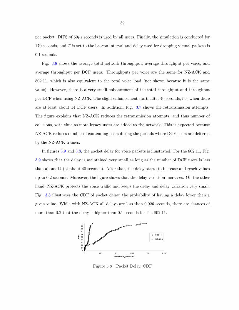
59
per packet. DIFS of 50µs seconds is used by all users. Finally, the simulation is conducted for
170 seconds, and T is set to the beacon interval and delay used for dropping virtual packets is
0.1 seconds.
Fig. 3.6 shows the average total network throughput, average throughput per voice, and
average throughput per DCF users. Throughputs per voice are the same for NZ-ACK and
802.11, which is also equivalent to the total voice load (not shown because it is the same
value). However, there is a very small enhancement of the total throughput and throughput
per DCF when using NZ-ACK. The slight enhancement starts after 40 seconds, i.e. when there
are at least about 14 DCF users. In addition, Fig. 3.7 shows the retransmission attempts.
The figure explains that NZ-ACK reduces the retransmission attempts, and thus number of
collisions, with time as more legacy users are added to the network. This is expected because
NZ-ACK reduces number of contending users during the periods where DCF users are deferred
by the NZ-ACK frames.
In figures 3.9 and 3.8, the packet delay for voice packets is illustrated. For the 802.11, Fig.
3.9 shows that the delay is maintained very small as long as the number of DCF users is less
than about 14 (at about 40 seconds). After that, the delay starts to increase and reach values
up to 0.2 seconds. Moreover, the figure shows that the delay variation increases. On the other
hand, NZ-ACK protects the voice traffic and keeps the delay and delay variation very small.
Fig. 3.8 illustrates the CDF of packet delay; the probability of having a delay lower than a
given value. While with NZ-ACK all delays are less than 0.026 seconds, there are chances of
more than 0.2 that the delay is higher than 0.1 seconds for the 802.11.
0
0.1
0.2
0.3
0.4
0.5
0.6
0.7
0.8
0.9
1
0 0.05 0.1 0.15 0.2 0.25
Packet Delay (seconds)
CD
F 802.11
NZ-ACK
Figure 3.8 Packet Delay, CDF

60
3.8 Conclusions
The 802.11e standard is designed to be backward compatible with the 802.11. As a re-
sult, wireless networks are expected to have a combination of both EDCA (802.11e Enhanced
Distributed Channel Access) and legacy DCF (802.11 Distributed Control Function) users.
Typically, the 802.11e users who have QoS requirements are supposed to get a higher priority
service than that of legacy users. However, the EDCA users’ performance may be degraded
because of the existence of legacy users, and therefore would get a lower priority service. The
main reason for such effects is due to the fact that EDCA users are controlled through the use
of different contention parameters (AIFS, CWmin, CWmax, TXOP) that are distributed via
the beacon frames. In contrast, there is no control over legacy users because their contention
parameters (DIFS, CWmin, CWmax) are PHY dependent, i.e. they have constant values. As
a result, depending on the network status like the number of DCF/EDCA users, DCF users
could achieve a higher priority and could result in high collision rates, and thus degrade the
performance of EDCA users.
In this chapter, we discussed different aspects of the legacy DCF and EDCA coexistence
and provided general desirable features for any mitigation solution. Based on those features, we
proposed a simple distributed management scheme, called NZ-ACK, to mitigate the influence
of legacy DCF on EDCA performance in networks that consist of both types of users. NZ-ACK
controls legacy users by introducing a new ACK policy in which the QAP is allowed to set the
duration of the last ACK in a transmission exchange to a non-zero value.
In addition, we presented strategies to determine when to issue such NZ-ACK frames, and
0
0.05
0.1
0.15
0.2
0 20 40 60 80 100 120 140 160 180
Time (seconds)
Packet
Dela
y (
seco
nd
s) 802.11
NZ-ACK
Figure 3.9 Packet Delay

61
the non-zero duration value of a NZ-ACK frame. All the processing of NZ-ACK scheme is
implemented at QAP. However, non-QAP EDCA users only are required to distinguish the
new ACK policy in order to ignore the non-zero value duration included in a NZ-ACK frame.
On the other hand, NZ-ACK requires no modification (i.e. fully transparent) to legacy users.
Thus, NZ-ACK maintains backward compatibility.
The proposed scheme allows EDCA users to start competing directly after NZ-ACK frames.
However, DCF users would defer their access to the channel according to the non-zero duration
of NZ-ACK frame. Moreover, when to issue NZ-ACK frames and their duration values are
determined adaptively according to network status. Thus, more resources for the EDCA users
are reserved in a dynamic and distributed fashion to maintain their priority. The performance
gain is due to the fact that NZ-ACK reduces the number of contending users when issuing
non-zero duration NZ-ACK frames; only EDCA users are competing for the channel when
DCF users are yielding. As a result, lower collision rates for both types of users are expected
and thus higher throughputs, fairness levels, and lower delays.
Finally, we used OpnetModeler to evaluate NZ-ACK and compare its performance to that
of 802.11 and ACKS. The results show that NZ-ACK outperforms the other two approaches in
terms of maintaining the priority of service and delay bounds of EDCA users while providing
acceptable throughput for legacy users.

62
CHAPTER 4. Turning Hidden Nodes into Helper Nodes in IEEE 802.11
Wireless LAN Networks
Submitted to the IEEE Transactions on Mobile Computing (TMC)
Haithem Al-Mefleh 1,3, J. Morris Chang 2,3
4.1 Abstract
To enhance the performance of IEEE 802.11 WLANs in the presence of hidden terminal
problem, we propose a protocol that allows non-hidden stations to help each other retransmit
faster whenever possible. Opposite to other approaches, the new protocol benefits from the
hidden terminal problem to improve the performance of DCF, which is the basic operation
of IEEE 802.11. The proposed protocol is compatible with IEEE 802.11, and works with the
same PHY of IEEE 802.11. We also provide an analytical model to evaluate the throughput of
the new scheme and compare it to that of DCF. The model is validated via Opnet simulation.
Using Opnet simulation, results show that the proposed scheme improves throughput, delay,
packet drop, retransmissions, and fairness with small trade-off regarding fairness depending on
the network topology.
4.2 Introduction
The IEEE 802.11 (3; 4; 13) wireless networks are widely deployed. Therefore, many chal-
lenges of the wireless medium are addressed by research especially to improve the performance
of the IEEE 802.11 DCF (Distributed Coordination Function), which is the basic operation of1Graduate student.2Associate Professor.3Department of Electrical and Computer Engineering, Iowa State University.

63
the medium access control (MAC) defined in IEEE 802.11. One major challenge is the hidden
terminal problem which significantly degrades the performance of DCF because it results in
high collision rates.
When a collision occurs, some stations other than the destination may be able to suc-
cessfully receive one of the collided packets. Reasons include the capture effect and hidden
terminal problem because of different locations of stations, existing obstacles like walls and
doors, and interferences. Accordingly, and different than other proposals, we would like to
investigate whether non-hidden stations could help each other retransmit faster whenever pos-
sible to enhance the performance of the 802.11 wireless local area networks (WLANs). In this
chapter, we propose a new simple protocol that modifies 802.11 DCF, is backward compatible,
and works over the 802.11 PHY to achieve such goal. We present an analytical model to study
the throughput performance of the new scheme and validate that model via simulation using
Opnet Modeler. We also evaluate the new scheme using Opnet with and without capture effect
for different topologies. Results show gains of retransmissions, throughput, fairness, delay, and
packet drops with a small trade-off regarding fairness in some scenarios.
The rest of the chapter is organized as following. In section 4.3 we provide background
information about the IEEE 802.11 DCF and hidden terminal problem, and then related works
are discussed in section 4.4. In section 4.5, we provide detailed description of the proposed
protocol. We then present an analytical model to analyze the throughput performance of the
proposed scheme in section 4.6. Simulation results are given in section 4.7 to validate the anal-
ysis model and provide performance evaluation of the proposed scheme. Finally, conclusions
are in section 4.8.
4.3 Background
In this section, we first introduce the IEEE 802.11 DCF, and then we discuss the the hidden
terminal problem.

64
4.3.1 IEEE 802.11 DCF
The IEEE 802.11 standard defines two mechanisms for DCF which are based on Carrier
Sense Multiple Access/Collision Avoidance (CSMA/CA). In basic operation, a station that has
a packet to transmit will do so if the medium is sensed idle for a period of distributed interframe
space (DIFS). Otherwise, the station will go into backoff where the Binary-Exponential-Backoff
(BEB) procedure is used. The station chooses a number of time slots to wait before trying to
transmit again. The number, or the backoff counter, is selected from the range [0, CW ], where
CW is called the contention window and is initially set to CWmin. The station decrements its
backoff counter by one for every slot time the medium is sensed idle. When the backoff counter
reaches zero, the station transmits its packet. Upon receiving a data frame, the destination
responds by sending back an acknowledgment (ACK) frame after a short interframe space
(SIFS) time. The ACK frame has a higher priority because SIFS is the shortest interframe
space (IFS) used in DCF. The packets transmitted carry the time needed to complete the
transmission of a packet and its acknowledgement. This time is used by all other stations to
defer their access to the medium and is called NAV, Network Allocation Vector. Collisions
occur when two or more stations are transmitting at the same time, or when the ACK frame is
not received after a timeout period. With every collision, the transmitting station will double
its CW unless it reaches a maximum limit CWmax, and selects a new backoff counter from the
new range. The process is repeated until the packet is successfully transmitted or is dropped
because a retry limit is reached.
In RTS/CTS operation, a station uses control frames to contend for the channel before
transmitting data frames, i.e. data frames are free of collision. When the backoff counter
reaches zero, the transmitter starts by sending RTS frame to the receiver who then replies with
CTS if RTS frame is received successfully. The durations of RTS and CTS frames are used to
reserve the channel long enough to exchange the following data frame and its acknowledgement.
Fig. 4.1 illustrates the RTS/CTS operation in a fully connected (no hidden nodes) network
WLAN.

65
Backoff SlotsSIFSRTS
Defer Access
DIFS
CTS
Backoff SlotsDIFS
AP
S1
Others
Data
ACK
SIFS SIFS
Figure 4.1 RTS/CTS operation without hidden nodes
AP
S3S1
S2
Figure 4.2 Hidden terminal problem
4.3.2 Hidden Terminal Problem
Using the wireless medium, a station is not able to hear frames transmitted by another
station when they are out of range. Such phenomenon is referred to as the hidden terminal
problem, and significantly degrades the performance of 802.11 DCF because it results in high
collision rates. An example is shown in Fig. 4.2 where S1 and S2 are within range, and are
hidden from S3. Just like when all stations are within range, collisions occur because of equal
backoff values used by different nodes. However, the hidden terminal problem adds another
type of collisions as shown in Fig. 4.3. Here, S1 and S3 are contending for the channel with
S1 backoff value is smaller than that of S3. Accordingly, S1 starts to transmit its RTS frame
to the AP (access point). Unfortunately, S3 is unaware of S1’s transmission and thus does not
freeze its backoff counter. S1’s RTS frame would not experience a collision only if S3’s backoff
counter reaches zero after the start of the response frame, i.e. a CTS frame from the AP.
However, here S3 backoff counter reaches zero sometime before the end of S1’s transmission,
and thus S3 starts transmitting its RTS frame. As a result, a collision occurs at the AP and
both station S1 and S3 would timeout and then double their contention windows.
Backoff SlotsRTS
DIFS
Backoff SlotsDIFS
AP
S1
S3RTS
Figure 4.3 Collision due to hidden terminal problem

66
A special situation occurs when S3 starts transmitting RTS frame at the same time the
AP may start transmitting CTS frame. Accordingly, S1 would start transmitting a data
frame. However, S3 would time out and begin backoff procedure. As a result, S3 may attempt
to retransmit while S1 is transmitting the data frame resulting in a collision of the data
frame. Consequently, data frames are not collision-free with RTS/CTS operation when hidden
terminal problem exists.
4.4 Related Work
There are few analytical models for wireless networks with hidden terminals like (14; 15; 16).
In (17), the authors analyze the effect of hidden terminal on the throughput of a WLAN AP.
They find that hidden terminal problem reduces the network throughput by 50%, and the
capture effect (receiving one of the collided frames correctly under some conditions (18; 19; 20;
21; 22)) can enhance the performance by (10 − 15)%. Capture effect adds to the complexity
and cost of wireless devices, and thus is mostly not implemented. In (23), a study of the effect
of hidden terminal problem in a multi-rate 802.11b network for both basic and RTS/CTS
methods is provided. The study shows that although RTS/CTS method does not help against
hidden nodes for rates higher than 1Mbps and 2Mbps, it is recommended for all rates since it
alleviates the packet collisions.
Different approaches are proposed to reduce the effect or/and the number of hidden nodes.
First, in many protocols like 802.11 DCF (3), the RTS/CTS exchange is used to mitigate
the hidden terminal problem. Second, the use of centralized scheduling like 802.11 PCF (3)
would help. However, scheduling is not attractive because of its higher complexity, centralized
control, and overhead of control packets which increase latency and reduce throughput. Third,
increasing the transmission power or the carrier-sensing range may reduce the number of hidden
nodes. In (22), the authors define a set of conditions for removing the hidden terminal problem
for 802.11 ad-hoc and infrastructure networks: 1) the use of a sufficiently large carrier-sensing
range, and 2) the use of capture effect which is referred to as the ”Restart Mode” of the
receiver. The authors show that one of these conditions alone is not sufficient; both conditions

67
are required. Moreover, the work assumes that there are no significant obstructions in the
network. In general, such approaches could be undesirable for energy-efficiency reasons, and
would increase the exposed nodes problem in overlapping WLANs and ad-hoc networks. In
addition, it may not be feasible due to different limits like available power levels, obstacles,
and regulations. On the contrary, power control schemes (24; 25) could result in increasing the
number of hidden nodes. Fourth, multi-channel approaches (26) mitigate the effect of hidden
stations. These approaches require more transceivers and channels, and more complex MAC
protocols. Fifth, busy tone protocols (27; 28) require a central node or a separate channel to
transmit a special signal to inform other nodes that there is an ongoing data transmission.
Finally, using new MACs and backoff algorithms, adapting the contention parameters, and
broadcasting helpful information are used (many of which do not consider the hidden-terminal
problem). In (29), each station broadcasts its backoff time in data frames to achieve fairness
with its neighbors, and a multiplicative increase/linear decrease backoff algorithm is used. In
(30), an impatient backoff algorithm is proposed to enhance the fairness level toward the nodes
in the middle of an ad-hoc network. In contrast to all existing approaches, impatient nodes
decrease their backoff upon a collision or losing contention, and increase it upon a successful
transmission using an exponential instead of a uniform random backoff. The authors assume
slotted system where synchronization is achieved, and propose to use reset messages to address
the issues of small backoff values when there are many collisions and high backoff values when
there are no collisions.
4.5 The Proposed Scheme
In the following, we first explain the motivation behind the proposed scheme. Then we
show the details of the new protocol, and discuss implementation issues.
4.5.1 Motivation
With the IEEE 802.11’s distributed operation of DCF, stations compete for the channel
using a random access scheme. Hence, there are always collisions whose level increases with

68
the number of contending stations, and the existence of hidden terminal problem. Different
approaches were proposed to enhance DCF by adjusting contention parameters and the backoff
procedure. However as discussed in related work (Section 4.4), they do not eliminate the hidden
terminal problem, or even do not consider it.
When a collision occurs because of hidden terminal problem, some stations other than the
destination may be able to successfully receive one of the collided packets. The same scenario
may occur if there is a bad channel between the transmitter and the destination, like existing
noise at destination, while there is a good channel between the transmitter and some stations
other than the destination. In the presence of hidden nodes, we would like to investigate if
non-hidden stations could help each other for retransmitting collided frames to enhance the
performance of infrastructure WLANs. Such cooperative retransmission is expected to be
faster since with DCF a non-collided station mostly transmits earlier than collided stations
that double their CW. First, we propose a new simple protocol that modifies 802.11 DCF, is
backward compatible, and works over the 802.11 PHY to achieve such goal. Then, we evaluate
the proposed protocol via simulation.
4.5.2 Description of the New Scheme
We distinguish between two types of transmission opportunities (TXOPs) as shown in
Fig. 4.4. First, a normal TXOP (NTXOP) occurs when a stations starts to transmit a data
frame after the required DIFS, or EIFS, and backoff periods. Second, a compensating TXOP
(CTXOP) occurs when a station starts to transmit after the current NTXOP by SIFS period.
Also, each station maintains locally a table, called CTABLE, of other stations that may need
to be assigned CTXOPs. When a station (say S2) overhears an RTS frame or a data from
another station (say S1) sent to the AP, it adds an entry (the MAC address) of the frame
transmitter (S1) to its CTABLE if no such entry exists. A station (S2) drops an existing entry
from local CTABLE when overhearing an ACK frame sent to another station (S1) whose MAC
address is equal to that entry. Note that a station is not required to wait for ACK frames after
RTS or data frame to add/remove an entry to/from its CTABLE.

69
Data
CACK
Data
ACK,
CF-END
S1
S2
AP
NTXOP CTXOP
SIFS
SIFS
SIFS
S3
DIFS+
Backoff
DIFS+
BackoffRTS
RTS
RTS
CTS
SIFS
SIFS
DIFS+
Backoff
DIFS+
Backoff
DIFS+
Backoff
DIFS+
Backoff
Figure 4.4 The proposed scheme
Fig. 4.4 illustrates the new scheme. Here, only S3 is hidden from both S1 and S2. After
DIFS and backoff periods following DCF operation, both S1 and S3 transmissions overlap
resulting in a collision. Since S2 overheard S1’s data frame, it adds S1’s MAC address to its
CTABLE. After backoff, S2 transmits without interference, and at the same time informs the
AP that S1 has a collided packet to transmit by including S1’s MAC address in the transmitted
data frame. The AP responds by sending back an ACK to S2 while piggybacking the AID of
S1 in this ACK frame (CACK frame in Fig. 4.4). Upon receiving the ACK frame, S2 remove
the entry of S1 from its CTABLE, S1 removes the entry of S2 from its CTABLE if exists, and
S1 recognize that it is assigned a CTXOP. Thereafter, S1 sends a data frame after a period
of SIFS to the AP who then replies with an ACK (last frame in Fig. 4.4). When overhearing
the ACK, S2 removes S1’s MAC address from its CTABLE, and all stations continue their
contention for the channel.
For reasons like power saving (energy will be consumed for every bit transmitted or re-
ceived), an 802.11 station first receives the MAC header of a frame and then receives the
payload only if the frame is destined to that station. This behavior is not changed by the
new scheme as only headers information is needed. Also, the helping station does not reserve
the channel for a CTXOP, but the AP does so using the duration value of the CACK frame.
Since duration is not known in advance, it is set to the time required to transmit a frame
with maximum possible length and lowest rate. If needed (duration reserved is longer than
CTXOP), the AP sends an ACK+CF-END frame instead of ACK frame in the CTXOP so
that all stations reset their NAV values to start contention. On the other hand, the AP sends
a CF-END if the helped station did not start transmitting after PIFS. Finally, when a station

70
Frame
ControlDuration RA
Octets: 2 62 4
FCS
Figure 4.5 ACK frame
Frame
ControlDuration RA CAID
Octets: 2 62 2
FCS
4
Figure 4.6 CACK frame
gets a CTXOP, it does not reset its CW value and it uses its current backoff counter for the
next frame in order to maintain adapting to congestion levels.
4.5.3 Capture Effect
Capture effect (18; 19; 20; 21; 22) allows receiving one of the collided frames correctly under
some conditions, and thus would enhance the throughout of the network while decreasing the
fairness level. Our scheme is expected to improve the performance of WLANs with or without
the hidden terminal problem when capture effect is enabled since more than one station is
included in a collision; using the proposed scheme, those transmissions not captured still can
be helped as different stations would capture different frames depending on the distance and
environment between each receiver and different transmitters.
4.5.4 Implementation Issues
4.5.4.1 CACK frame
A CACK is a new ACK type with a format shown in Fig. 4.6, and adds only one field,
named CAID, to that standard ACK frame shown in Fig. 4.5. CAID represents the AID of
the station that is assigned a CTXOP following the current NTXOP. The 16-bit AID is used
because of its smaller size compared to that of the 48-bit MAC address, and thus reducing the
extra time required.
To distinguish between ACK and CACK frames, we used the fact that all bits B8 to B15
except for B12 in the Frame Control field of IEEE 802.11 control frames are always set to
′0′. In our implementation, we selected B10 to be set to ′1′ for CACK. Note that a CTS
frame also can be used with the same modifications to implement a CACK. The new scheme
is fully backward compatible since CACK is of known type and subtype, and will not be used
to acknowledge data frames from stations that do not implement the new scheme.

71
4.5.4.2 Data frames
Data frames are not changed. AIDs cannot be used here becuase a non-AP station main-
tains only its own AID. Hence, the 48-bit ”Address4” of the IEEE 802.11 data frame’s header
can be used by a station to inform the AP about a collided station.
4.6 Analysis
Here, we present an analytical model for an infrastructure network where hidden terminal
problem exists. First, we provide general analysis for the network throughput, and then focus
on a specific topology.
In our analysis, we assume saturation conditions where users always have some data packets
to transmit. In addition, we assume ideal channel with collisions being the only source of errors.
Finally, we consider RTS-CTS operation of DCF.
4.6.1 Channel State
As shown in Fig. 4.7, generally the channel can be in one of three states: idle, success, and
collision. Idle state refers to the time spent in backoff; i.e. no transmission from any user. On
the other hand, a transmission can be a collision or a successful one. While the success state
refers to the time used for sending a data frame correctly, the collision state refers to the time
needed to send a data frame incorrectly due to overlapping with at least another transmission.
IDLE Colision IDLE Success IDLE Success
Figure 4.7 Channel state
Each idle period consists of a number of time slots. Fig. 4.8 illustrates the time spent in a
collision or a successful transmission in IEEE 802.11 DCF with RTS-CTS enabled. A successful
state occurs when there is only one user transmitting at a time, or when there is a collision
with one RTS frame is captured. However, a collision happens when more than one user are
transmitting at the same time and none of the transmitted RTS frames can be captured.

72
DataRTS CTS ACKSIFS SIFS SIFS DIFS
CollisionRTS
DIFS
Success
Tc
Ts
Figure 4.8 Success and collision times in DCF with RTS-CTS
DataRTS CTS CACKSIFS DIFSSIFS SIFS SIFS
Data ACKSIFS
Success/
Help
Th
DataRTS CTS ACKSIFS SIFS SIFS DIFS
Success/
No helpTs
Te
CollisionRTS
DIFS
Tc
Figure 4.9 Success and collision times in DCF with RTS-CTS when thenew scheme is enabled
When the proposed scheme is enabled, the channel also can be in one of the three states
as discussed above. However, a successful transmission can be of two possible lengths. The
successful transmission can be of the same length as that in a normal DCF operation, or may
occur as shown in Fig. 4.9. The normal operation occurs when the transmitting user has an
empty CTABLE (i.e. no one to help), and the new type happens when the transmitting user
has a non-empty CTABLE (i.e. at least one other user to help).
4.6.2 Throughput and Throughput Gain
Consequently, the average throughput of DCF (SDCF ) can be described by the formula:
SDCF =PsuccessL
Pidleσ + PsuccessTs + PcollisionTc(4.1)
where L is the average data frame size, Psuccess is the probability of a successful transmission,
Pcollision is the probability of collision, and Pidle is the probability of idle periods, σ is the time
slot length, Ts is the time of a successful transmission, and Tc is the time of a collision.
Since the new scheme does not change the backoff counter after a CTXOP, the average
throughput of the new scheme (SH) is given by equation (4.2) where Phelp is the probability

73
SH =PsuccessPhelp(2L) + Psuccess(1− Phelp)L
Pidleσ + Psuccess(1− Phelp)Ts + PsuccessPhelpTh + PcollisionTc
=Psuccess(1 + Phelp)L
Pidleσ + Psuccess(1− Phelp)Ts + PsuccessPhelpTh + PcollisionTc(4.2)
that the transmitting station would help another user, and Th is the time of a successful
transmission when a help occurs. Therefore, PsuccessPhelp is the probability of a successful
transmission with help taking place, and Psuccess(1 − Phelp) is the probability of a successful
transmission without any help.
The following equations define different times, see Fig. 4.8 and Fig. 4.9.
Ts = TRTS + TCTS + TData + TACK + 3SIFS + DIFS (4.3)
Tc = TRTS + DIFS (4.4)
Th = TRTS + TCTS + TData + TCACK + TData +
TACK + 5SIFS + DIFS
= Ts + TData + TCACK + 2SIFS (4.5)
We also define Te as the extra time when a successful transmission with help occurs.
Th = Ts + Te (4.6)
i.e. Te = TData + TCACK + 2SIFS.
Then, SH becomes:
SH =Psuccess(1 + Phelp)L
Pidleσ + PsuccessTs + PsuccessPhelpTe + PcollisionTc(4.7)
From equations (4.1) and (4.7), we can find the throughput ratio R (i.e. SHSDCF
) and the
throughput gain defined by G× 100% where G is SH−SDCFSDCF
or R− 1
R =(1 + Phelp)T
T + PsuccessPhelpTe(4.8)
G =Phelp(T − PsuccessTe)T + PsuccessPhelpTe
(4.9)

74
where T = Pidleσ + PsuccessTs + PcollisionTc.
From equations (4.8) and (4.9), it follows that:
1. Since (T − PsuccessTe) > 0, then G ≥ 0. In other words, there is no degradation of the
network throughput; i.e. the throughput of the network is at least equal to that of DCF
without the new scheme (R ≥ 1).
2. There is no gain when help is not possible; i.e. G = 0 and R = 1 when Phelp = 0. Such
scenario occurs when the topology of the network does not allow for nodes to help each
other. An example is a network of fully connected nodes with capture effect not utilized.
3. Note that (T − PsuccessTe)Phelp < (T + PsuccessPhelpTe). Accordingly, the throughput
gain is always less than 100% (i.e. 0 ≤ G < 1, and 1 ≤ R < 2).
4.6.3 Throughput Analysis
To find the network throughput, we need to solve different probabilities (Pidle, Psuccess,
Pcollision, and Phelp). We use the analysis model of (2) as it is known to be simple and correct.
To summarize, the analysis model is based on solving the non-linear system of equations (4.10)
and (4.11).
τ =2(1− 2ρ)
(1− 2ρ)(W + 1) + Wρ(1− (2ρ)r))(4.10)
ρ = 1− (1− τ)n−1 (4.11)
where n is the total number of contending users, W is CWmin, r is the maximum backoff
stage (CWmax = 2rW ), τ is the probability that a station transmits in any slot time, and ρ
is the conditional probability that the transmitted packet will collide. Accordingly, Ptr is the
probability of a transmission, and Ps is the probability that a transmission is successful given
that there is exactly one transmitter
Ptr = 1− (1− τ)n (4.12)
Ps =nτ(1− τ)n−1
Ptr(4.13)
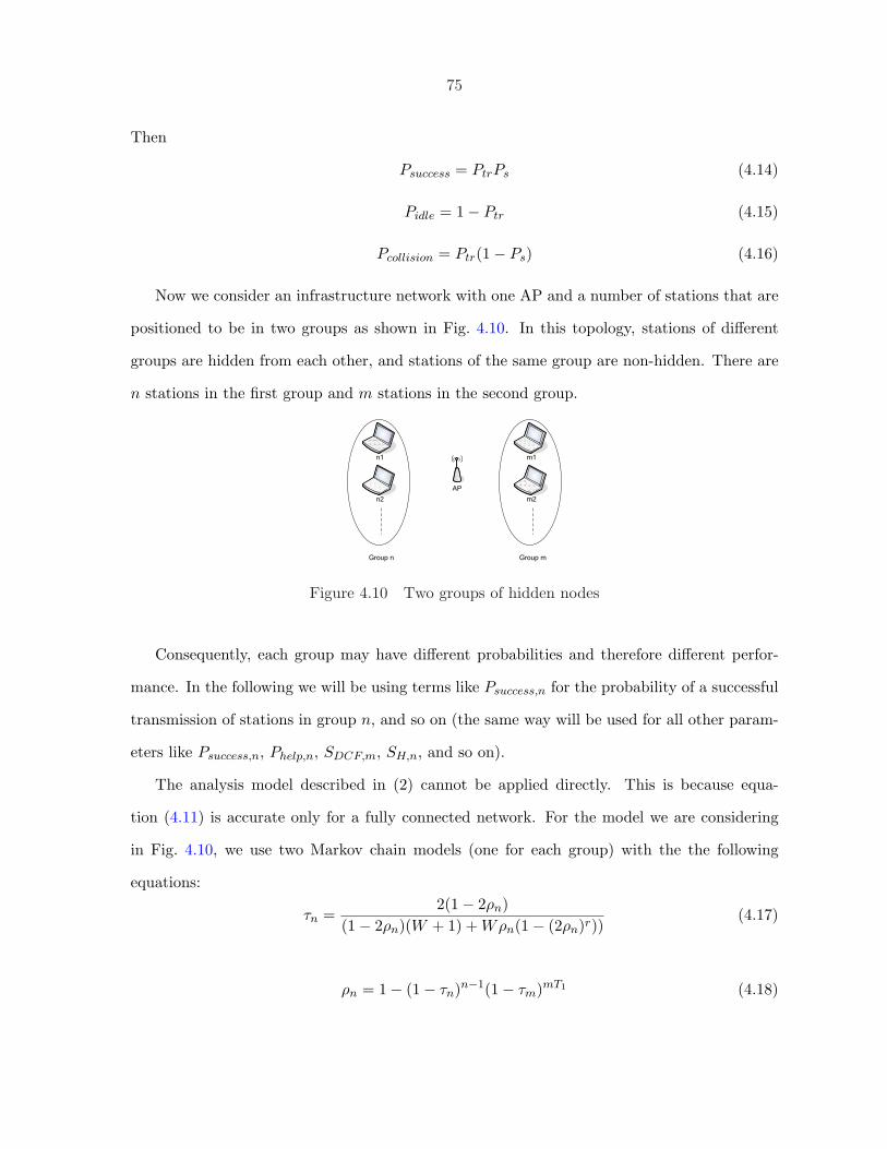
75
Then
Psuccess = PtrPs (4.14)
Pidle = 1− Ptr (4.15)
Pcollision = Ptr(1− Ps) (4.16)
Now we consider an infrastructure network with one AP and a number of stations that are
positioned to be in two groups as shown in Fig. 4.10. In this topology, stations of different
groups are hidden from each other, and stations of the same group are non-hidden. There are
n stations in the first group and m stations in the second group.
AP
n1
Group n
n2
m1
Group m
m2
Figure 4.10 Two groups of hidden nodes
Consequently, each group may have different probabilities and therefore different perfor-
mance. In the following we will be using terms like Psuccess,n for the probability of a successful
transmission of stations in group n, and so on (the same way will be used for all other param-
eters like Psuccess,n, Phelp,n, SDCF,m, SH,n, and so on).
The analysis model described in (2) cannot be applied directly. This is because equa-
tion (4.11) is accurate only for a fully connected network. For the model we are considering
in Fig. 4.10, we use two Markov chain models (one for each group) with the the following
equations:
τn =2(1− 2ρn)
(1− 2ρn)(W + 1) + Wρn(1− (2ρn)r))(4.17)
ρn = 1− (1− τn)n−1(1− τm)mT1 (4.18)

76
τm =2(1− 2ρm)
(1− 2ρm)(W + 1) + Wρm(1− (2ρm)r))(4.19)
ρm = 1− (1− τm)m−1(1− τn)nT1 (4.20)
where T1, shown in Fig. 4.11, is the time, normalized to the number of time slots in the
equations or 2TRTS+2SIFSσ , during which a transmission from a hidden node may start during
the ongoing transmission. We consider that a collision occurs whenever there is an overlap
between transmitted frames from different stations. The non-linear system of equations (4.17)-
(4.20) can be solved numerically.
RTS
RTS
(1 or more)
RTS
(1 or more)
T1
SIFSSIFS
Figure 4.11 Time during which a collision due to hidden stations may occur
Accordingly, we can find the following probabilities
Ptr,n = 1− (1− τn)n (4.21)
Ptr,m = 1− (1− τm)m (4.22)
Ps,n =nτn(1− τn)n−1(1− τm)mT1
Ptr,n(4.23)
Ps,m =nτm(1− τm)m−1(1− τn)nT1
Ptr,m(4.24)
Hence,
Pidle,n = 1− Ptr,n (4.25)
Psuccess,n = Ptr,nPs,n (4.26)
Pcollision,n = Ptr,n(1− Ps,n) (4.27)
Pidle,m = 1− Ptr,m (4.28)
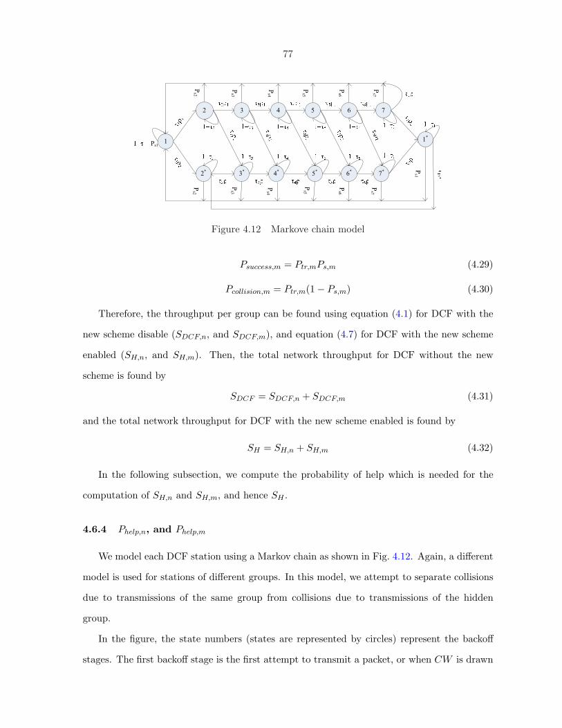
77
Ps7
Ps6
Ps5
Ps4
Ps3
Ps2
Ps1
Ps7
Ps6
Ps5
Ps4
Ps3
Ps2
Ps1
1
2 3 4 5 6 7
2*
3*
4*
5*
6*
7*
1*
Figure 4.12 Markove chain model
Psuccess,m = Ptr,mPs,m (4.29)
Pcollision,m = Ptr,m(1− Ps,m) (4.30)
Therefore, the throughput per group can be found using equation (4.1) for DCF with the
new scheme disable (SDCF,n, and SDCF,m), and equation (4.7) for DCF with the new scheme
enabled (SH,n, and SH,m). Then, the total network throughput for DCF without the new
scheme is found by
SDCF = SDCF,n + SDCF,m (4.31)
and the total network throughput for DCF with the new scheme enabled is found by
SH = SH,n + SH,m (4.32)
In the following subsection, we compute the probability of help which is needed for the
computation of SH,n and SH,m, and hence SH .
4.6.4 Phelp,n, and Phelp,m
We model each DCF station using a Markov chain as shown in Fig. 4.12. Again, a different
model is used for stations of different groups. In this model, we attempt to separate collisions
due to transmissions of the same group from collisions due to transmissions of the hidden
group.
In the figure, the state numbers (states are represented by circles) represent the backoff
stages. The first backoff stage is the first attempt to transmit a packet, or when CW is drawn

78
from the range [0, CWmin − 1]. After each collision, the station moves to the next backoff
stage with the new range [0, 2iCWmin] where i is the number of the backoff stage. When i is
more than r (the maximum allowed backoff stage) where no change is made to the contention
window’s range. Here, we assume r = 5, and the maximum number of retries is 7. Also in
Fig. 4.12, τi is the probability of transmission when the station is at state i, Psi is the probability
of successful transmission when the station is at state i, ρ1 is the conditional probability of
collisions due transmissions of the same group, and ρ2 is the conditional probability of collisions
due to transmissions of the hidden group. Finally, we use two different types of each backoff
stage. A station cannot be helped if it is in state i ∈ (1, 2, ..., 7). On the other hand, the
station may be helped if it is in state i ∈ (1∗, 2∗, ..., 7∗).
τi =2
1 + 2i−1CWmin(4.33)
Psi = τi(1− ρ) (4.34)
ρn,1 = 1− (1− τn)n−1 (4.35)
ρn,2 = (1− (1− τm)mT1)(1− τn)n−1 (4.36)
ρm,1 = 1− (1− τm)m−1 (4.37)
ρm,2 = (1− (1− τn)nT1)(1− τm)m−1 (4.38)
Note that τi∗ = τi, Psi = Psi∗ , ρm = ρm,1 + ρm,2, and ρn = ρn,1 + ρn,2. Also, we already can
calculate these probabilities using the values of τn and τm found in subsection 4.6.3.
We now solve the Markov chain model in Fig. 4.12 in general for both groups. By letting
πi be the probability of being in state i, the following holds in the Markov chain model
7∑
i=1
(πi + πi∗) = 1 (4.39)
πi = πi−1τi−1ρ1 + πi(1− τi)
=τ1ρ
i1
τiπ1, i = 2, 3, ..., 7. (4.40)

79
πi∗ = πi∗−1τi−1ρ + πi−1τi−1ρ2 + πi∗(1− τi)
=πi∗−1τi−1ρ + πi−1τi−1ρ2
τi, i = 2∗, 3∗, ..., 7∗. (4.41)
π1 =7∑
i=2
(πiPsi + πi∗Psi) + π7∗Ps7 + π7τ7ρ1
+π1(1− τ1)
=∑7
i=2(πiPsi + πi∗Psi) + π7∗Ps7 + π7τ7ρ1
τ1 − Ps1(4.42)
π1∗ = π7∗τ7ρ + π7τ7ρ2 + π1∗(1− τ1)
=π7∗τ7ρ + π7τ7ρ2
τ1(4.43)
Solving the above equations
π1∗ = απ1 (4.44)
where α = ρ2ρ6+ρ5ρ1+ρ4ρ2
1+ρ3ρ31+ρ2ρ4
1+ρρ51+ρ6
11−ρ7 . Hence, the probability of every state can be ex-
pressed as a function of π1 using equations (4.41) and (4.40). Thus we first find π1 using
equation (4.39) or (4.42), and then we calculate the probability of all other states.
Now we illustrate how to estimate the probability of help. Assume that a station of group
n can help another station within the same group with the probability ηn. A station can be
helped only when all the following conditions are true: 1) the station is in state i ∈ 1∗, 2∗, ..., 7∗,
2) the station was not helped while in the current state, and 3) the station was not helped in
another state j ∈ 1∗, 2∗, ..., 7∗ and moved to the current state i 6= j after collisions due to only
transmissions from stations of the same group. Then assuming a constant probability of help
and for given state i∗, we approximate ηn by π∗i - π∗i ηn -∑7
j=1,j 6=i π∗j ηn (the third part of this
expression is the approximated one). Then summing up over all states, we get
ηn =7∑
i=1
ηn,i∗
= 1−∑7
i=1 ηn,iπi∗
1 +∑7
i=1 7πi∗(4.45)
Then
Phelp,n = 1− (1− ηn)n−1 (4.46)

80
Table 4.1 Network Parameters
Parameter Value Parameter Value
Slot T ime 20µs MAC ACK Size 14 Bytes
SIFS 10µs MAC CTS Size 14 Bytes
DIFS 50µs MAC RTS Size 20 Bytes
CWmin 32 PLCP Overhead 192µs
CWmax 1023 DCF MAC Overhead 28 Bytes
Control Rate 1Mbps Short Retry Limit 4Data Rate 11Mbps Long Retry Limit 7
where ηn,i∗ is the probability of help given state i∗, and (1− ηn)n−1 is the probability that all
other n− 1 stations cannot be helped. Note that there is no need to include the hidden nodes,
i.e. stations in group m, since they cannot be helped by any station in group n.
Similarly, we can estimate ηm and then
Phelp,m = 1− (1− ηm)m−1 (4.47)
4.7 Performance Evaluation
This section presents the simulation we used to evaluate the performance of the proposed
scheme and compare it to that of 802.11 DCF. We implemented the new scheme with the
commercial Opnet Modeler 11.5.A (1) by modifying the Opnet 802.11 models. We consider an
infrastructure network which consists of one AP and a number of stations that share a single
wireless channel. Moreover, there are no channel errors; collisions are the only source of errors.
For each scenario, the results are the average of 100 different runs with a different seed, which
is used for the random generator, for each run. Finally, 802.11b and RTS/CTS operation are
used with the parameters shown in Table 4.1.
4.7.1 Performance Metrics
For performance analysis, we use the following metrics:
1. Throughput (S): the total data bits transmitted successfully per the simulation time.

81
2. Fairness Index (FI): we used Jain Index (12) defined by (FI = (∑n
i=1 Si)2
n∑n
i=1 S2i), where n is
number of stations and Si is the throughput of station i. The closer the value of FI to
1, the better the fairness provided. We use FI to find how fair a scheme is to different
DCF users.
3. Average Delay: the delay of a data packet is measured from the moment it was generated
until it is successfully received. Only successfully transmitted packets are considered for
finding the average delay.
4. Packet drop: number of data packets dropped due to buffers overflow, and due to reaching
a retry limit.
5. Retransmissions: the number of retransmission attempts of each packet before it is
successfully transmitted or dropped.
4.7.2 Hidden Groups without Capture Effect
Here, each scenario is an infrastructure network with one AP and a number of stations
that are positioned to be in two groups, see Fig. 4.10. Stations of different groups are hidden
from each other, and stations of same group are non-hidden. Each scenario is referred to
as n-m, with n stations in the first group and m stations in the second group, and n is
fixed while m is variable. Then we test with scenarios referred to as n-m-c, where a third
group (group c) of 5 stations, which are not hidden from each other, is added to each of the
previous n-m networks. However, stations of group c are arranged as following: 1) c1 and c2
are non-hidden from all stations in network. 2) c3 − {n2}. 3) c4 − {n1,m1,m5,m9,m10}. 4)
c5 − {m1, m5,m6,m7,m9,m10}. Here, xi is station i in group x, and xi − {xj} means that xi
and xj are hidden from each other. Also, |x| is used to refer to the number of stations in group
x. These scenarios include a general topology of a wireless network. Results are provided in
Fig. 4.13 to Fig. 4.22. In all figures, the letter ”d” (”e”) is used if the new scheme is disabled
(enabled).
For the n-m scenarios, different measures follow the same trend for DCF with the new

82
3.35
3.4
3.45
3.5
3.55
3.6
3.65
3.7
0 2 4 6 8 10 12mS
Mb
ps
0
0.1
0.2
0.3
0.4
0.5
0.6
0.7
0.8
0.9
1
FI
S 1-m d S 1-m e FI 1-m d FI 1-m e
Figure 4.13 Scenario 1-m
3
3.1
3.2
3.3
3.4
3.5
3.6
3.7
0 5 10 15
m
S M
bp
s
0
0.2
0.4
0.6
0.8
1
1.2
FI
S 2-m d S 2-m e FI 2-m d FI 2-m e
Figure 4.14 Scenario 2-m
2.9
3
3.1
3.2
3.3
3.4
3.5
3.6
3.7
0 5 10 15
m
S M
bp
s
0
0.2
0.4
0.6
0.8
1
1.2
FI
S 3-m d S 3-m e FI 3-m d FI 3-m e
Figure 4.15 Scenario 3-m

83
2.5
2.7
2.9
3.1
3.3
3.5
3.7
3.9
0 5 10m
S M
bp
s
0
0.2
0.4
0.6
0.8
1
1.2
FI
S 5-m d S 5-m e FI 5-m d FI 5-m e
Figure 4.16 Scenario 5-m
2
2.2
2.4
2.6
2.8
3
3.2
3.4
3.6
3.8
0 5 10m
S M
bp
s
0
0.2
0.4
0.6
0.8
1
1.2
FI
S 10-m d S 10-m e FI 10-m d FI 10-m e
Figure 4.17 Scenario 10-m
scheme enabled or disabled; we show this for fairness and throughput in Fig.4.13 to Fig.4.17.
This can be explained by the fact that CW resetting and backoff counters are unchanged after
a CTXOP. Fig. 4.13 to Fig. 4.17 also show a trade-off between throughput and fairness for the
n-m scenarios. The fairness gets smaller for some cases when the new scheme is enabled. This
is because collided stations may retransmit before being helped due to random backoff values.
However, the difference is small and FI of the new scheme is always above 0.7, and almost is
the same as that of DCF for the 1-m, and 10-m scenarios. On the other hand, fairness is always
enhanced for the n-m-c scenarios, Fig. 4.18 and Fig. 4.19, where there is higher probability
of being helped before retransmitting using contention due to more general relations (not just
two groups).
Fig. 4.13 to Fig. 4.19 illustrate that throughput is always enhanced. The minimum (max-
imum) gains (%) are about 3.2 (4.3), 3.1 (11.1), 3.9 (17.4), 4.1 (27.8), 4.3 (52.7), 1.8 (6.4),

84
3.28
3.33
3.38
3.43
3.48
3.53
3.58
3.63
3.68
0 5 10
m
S M
bp
s
0.5
0.55
0.6
0.65
0.7
0.75
0.8
0.85
FI
S 1-m-c d S 1-m-c e
FI 1-m-c d FI 1-m-c e
Figure 4.18 Scenario 1-m-c
3.28
3.33
3.38
3.43
3.48
3.53
3.58
3.63
3.68
0 5 10
m
S M
bp
s
0.5
0.55
0.6
0.65
0.7
0.75
0.8
FI
S 2-m-c d S 2-m-c e
FI 2-m-c d FI 2-m-c e
Figure 4.19 Scenario 2-m-c
0
2
4
6
8
10
12
14
16
18
20
0 2 4 6 8 10m
Gain
(%
)
1-m 2-m 3-m 5-m
10-m 2-m-c 1-m-c
Figure 4.20 Delay

85
0
5
10
15
20
25
30
35
40
0 2 4 6 8 10m
Gain
(%
)
1-m 2-m 3-m 5-m
10-m 2-m-c 1-m-c
Figure 4.21 Retransmissions
0
10
20
30
40
50
60
70
80
90
0 2 4 6 8 10m
Gain
(%
)
1-m 2-m 3-m 5-m
10-m 2-m-c 1-m-c
Figure 4.22 Packet drop
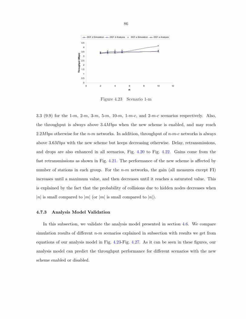
86
0
0.5
1
1.5
2
2.5
3
3.5
4
4.5
0 2 4 6 8 10 12
m
Th
rou
gh
pu
t (M
bp
s)
DCF d Simulation DCF d Analysis DCF e Simulation DCF e Analysis
Figure 4.23 Scenario 1-m
3.3 (9.9) for the 1-m, 2-m, 3-m, 5-m, 10-m, 1-m-c, and 2-m-c scenarios respectively. Also,
the throughput is always above 3.4Mbps when the new scheme is enabled, and may reach
2.2Mbps otherwise for the n-m networks. In addition, throughput of n-m-c networks is always
above 3.6Mbps with the new scheme but keeps decreasing otherwise. Delay, retransmissions,
and drops are also enhanced in all scenarios, Fig. 4.20 to Fig. 4.22. Gains come from the
fast retransmissions as shown in Fig. 4.21. The performance of the new scheme is affected by
number of stations in each group. For the n-m networks, the gain (all measures except FI)
increases until a maximum value, and then decreases until it reaches a saturated value. This
is explained by the fact that the probability of collisions due to hidden nodes decreases when
|n| is small compared to |m| (or |m| is small compared to |n|).
4.7.3 Analysis Model Validation
In this subsection, we validate the analysis model presented in section 4.6. We compare
simulation results of different n-m scenarios explained in subsection with results we get from
equations of our analysis model in Fig. 4.23-Fig. 4.27. As it can be seen in these figures, our
analysis model can predict the throughput performance for different scenarios with the new
scheme enabled or disabled.
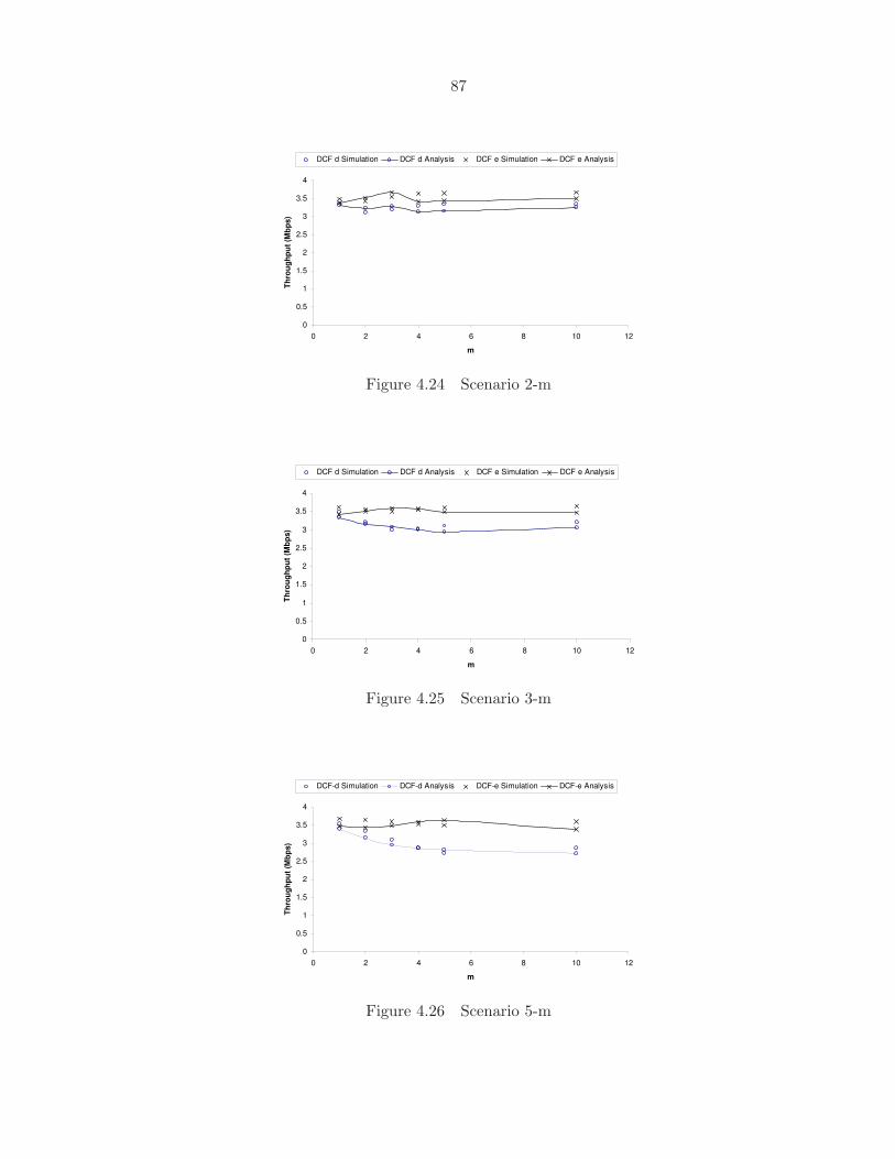
87
0
0.5
1
1.5
2
2.5
3
3.5
4
0 2 4 6 8 10 12
m
Th
rou
gh
pu
t (M
bp
s)
DCF d Simulation DCF d Analysis DCF e Simulation DCF e Analysis
Figure 4.24 Scenario 2-m
0
0.5
1
1.5
2
2.5
3
3.5
4
0 2 4 6 8 10 12
m
Th
rou
gh
pu
t (M
bp
s)
DCF d Simulation DCF d Analysis DCF e Simulation DCF e Analysis
Figure 4.25 Scenario 3-m
0
0.5
1
1.5
2
2.5
3
3.5
4
0 2 4 6 8 10 12
m
Th
rou
gh
pu
t (M
bp
s)
DCF-d Simulation DCF-d Analysis DCF-e Simulation DCF-e Analysis
Figure 4.26 Scenario 5-m
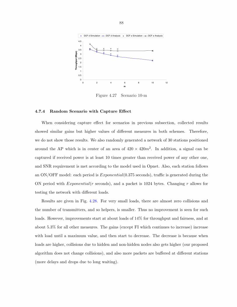
88
0
0.5
1
1.5
2
2.5
3
3.5
4
4.5
0 2 4 6 8 10 12
m
Th
rou
gh
pu
t (M
bp
s)
DCF d Simulation DCF d Analysis DCF e Simulation DCF e Analysis
Figure 4.27 Scenario 10-m
4.7.4 Random Scenario with Capture Effect
When considering capture effect for scenarios in previous subsection, collected results
showed similar gains but higher values of different measures in both schemes. Therefore,
we do not show those results. We also randomly generated a network of 30 stations positioned
around the AP which is in center of an area of 420 × 420m2. In addition, a signal can be
captured if received power is at least 10 times greater than received power of any other one,
and SNR requirement is met according to the model used in Opnet. Also, each station follows
an ON/OFF model: each period is Exponential(0.375 seconds), traffic is generated during the
ON period with Exponential(r seconds), and a packet is 1024 bytes. Changing r allows for
testing the network with different loads.
Results are given in Fig. 4.28. For very small loads, there are almost zero collisions and
the number of transmitters, and so helpers, is smaller. Thus no improvement is seen for such
loads. However, improvements start at about loads of 14% for throughput and fairness, and at
about 5.3% for all other measures. The gains (except FI which continues to increase) increase
with load until a maximum value, and then start to decrease. The decrease is because when
loads are higher, collisions due to hidden and non-hidden nodes also gets higher (our proposed
algorithm does not change collisions), and also more packets are buffered at different stations
(more delays and drops due to long waiting).

89
0
20
40
60
80
100
120
0 20 40 60 80 100 120
Load (%)
Gain
(%
)
FI S Delay Retransmissions Packet Drop
Figure 4.28 Performance gain for random scenario with capture effect
4.8 Conclusions
We proposed a new protocol for 802.11 WLANs to take advantage of the hidden terminal
problem by allowing non-hidden stations to assist each other retransmit faster whenever pos-
sible. The new scheme is a modification to DCF, is backward compatible, and works over the
802.11 PHY. We also presented an analysis model to calculate the saturation throughput of the
new scheme and compare it to that of DCF. We evaluated the proposed scheme and validated
the analytical model via simulation which was conducted using Opnet Modeler for different
scenarios. Results showed that the new scheme improves the throughput, delay, packet drop,
fairness, and retransmissions. The performance gain comes from cooperative retransmissions
that are faster than that used in DCF where a collided station doubles its CW. In addition,
results showed a trade-off between throughput and fairness only in some scenarios. Further
work includes investigating performance enhancements using different design issues like having
the AP decide when not to allow stations to assist each other, and using help information to
update backoff counters and CW.

90
CHAPTER 5. Maintaining Priority among IEEE 802.11/802.11e Devices
Modified from a paper submitted to the IEEE Transactions on Mobile Computing (TMC)
Haithem Al-Mefleh 1,3, J. Morris Chang 2,3
5.1 Introduction
In chapter 3, we proposed a simple distributed management scheme, called Non-Zero Ac-
knowledgement (NZ-ACK), to mitigate the influence of legacy DCF on EDCA performance
in networks consisting of both types of users without any modifications to legacy users. In
chapter 3, we used an intuition approach to address the main challenges of NZ-ACK: when
to issue NZ-ACK frames, and how long should be the duration of a NZ-ACK frame. In such
approach, we only considered the number of users of each type and the utilization required
by each EDCA user. Also, the approach presented in chapter 3 requires that the AP keeps a
buffer (called virtual buffer) for every EDCA user and maintains that buffer according to the
user requirements. Maintenance of buffers includes adding and dropping virtual packets.
In this chapter, we revise and extend the work presented in chapter 3. We modify NZ-ACK
protocol. First, virtual buffers are no longer needed. Second, we provide a model for solving
the main challenges of NZ-ACK such that we maintain the priority of EDCA users. We include
contention parameters (the contention window), number of users, and transmission activities of
both types of users. Third, we consider different ratios of DCF and EDCA users in evaluation.
This chapter starts with the analytical model in section 5.2. Then, evaluation of the
new approach is provided in 5.3. Finally, 5.4 gives collision remarks. Refer to chapter 3 for1Graduate student.2Associate Professor.3Department of Electrical and Computer Engineering, Iowa State University.

91
background information and problem statement.
5.2 Analysis
In this section, we address how the QAP determines when to issue NZ-ACK frames, and
how long is the duration of a NZ-ACK frame.
Assume there are n legacy DCF users in the network. For every user i (i = 1, ..., n), let
Xi be a discrete random variable representing the number of backoff slots selected following
a uniform distribution in the range from 0 to W − 1 (i.e. Xi ∼ U [0,W − 1], and W is the
minimum CW for DCF). Note that:
fXi(x) = P (Xi = x) =1W
; x = 0, 1, ...,W − 1 (5.1)
In addition, note that all Xi random variables are identical and independent.
fX1X2...Xn(x1, x2, .., xn) = fX1(x1)fX2(x2)...fXn(xn) (5.2)
The minimum backoff value selected by any DCF user is also a random variable XDCF :
XDCF = min(X1, X2, ..., Xn) (5.3)
The distribution function fXDCF(x) can be found by finding the probability P (XDCF = x),
for each x = 0, 1, 2, ...,W − 1.
P (XDCF = x) =
P (X1 = x,X2 ≥ x,X3 ≥ x,X4 ≥ x, ..., Xn ≥ x)
+P (X1 > x, X2 = x,X3 ≥ x,X4 ≥ x, ..., Xn ≥ x)
+P (X1 > x, X2 > x, X3 = x,X4 ≥ x, ..., Xn ≥ x)
+...
+P (X1 > x, X2 > x, X3 > x,X4 > x, ..., Xn = x) (5.4)
After some processing of equations (5.1), (5.2), and (5.4), it can be found that:
P (XDCF = x) =
gn−yn
W n ; x = 0, 1, ...,W − 1
0 ; otherwise(5.5)

92
ACK DCF
EDCAXEDCA
XDCF
DIFS
AIFS
XEDCA+AIFS-DIFS
Figure 5.1 Expected CWmin
where g = W − x, and y = W − x − 1. Therefor, the expected value of XDCF can be
calculated:
E[XDCF ] =W−1∑
x=0
xP (XDCF = x)
=
W−1∑x=1
xgn −W−1∑x=1
xyn
Wn
=1
Wn
W−1∑
x=1
xn
(5.6)
These formulas also can be used to find XEDCAj for each EDCA access category j (j =
0, 1, 2, 3; where access category 3 has the highest priority).
E[XEDCAj ] =1
Wjn
Wj−1∑
x=1
xnj (5.7)
where Wj is the minimum CW for access category j. Accordingly, we define E[XEDCA]
as the maximum of all E[XEDCAj ], AIFS as the corresponding AIFSj , and W ∗ as the corre-
sponding Wj . Since we are interested in maintaining service guarantees to the real time (voice
and video) access categories, we only consider access categories 3 and 2.
Consequently, we set the duration of an NZ-ACK frame to:
d =
0 ; D ≤ −1
1 ; − 1 < D < 1
dDe ; D < W ∗
W ∗ ; D ≥ W ∗
(5.8)
where
D = E[XDCF ]− E[XEDCA] + DIFS −AIFS (5.9)
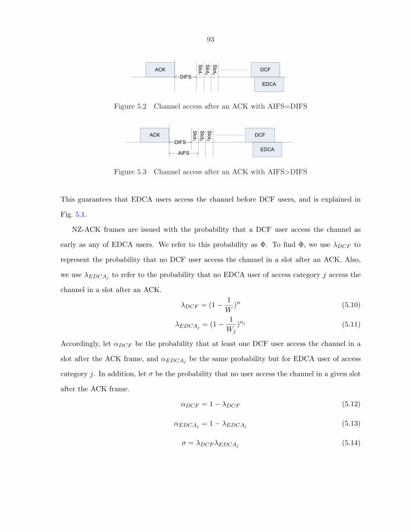
93
ACK DCF
EDCA
DIFS
Slot1
Slot2
Slot3
Figure 5.2 Channel access after an ACK with AIFS=DIFS
ACK DCF
DIFS
AIFSEDCA
Slot1
Slot2
Slot3
Figure 5.3 Channel access after an ACK with AIFS>DIFS
This guarantees that EDCA users access the channel before DCF users, and is explained in
Fig. 5.1.
NZ-ACK frames are issued with the probability that a DCF user access the channel as
early as any of EDCA users. We refer to this probability as Φ. To find Φ, we use λDCF to
represent the probability that no DCF user access the channel in a slot after an ACK. Also,
we use λEDCAj to refer to the probability that no EDCA user of access category j access the
channel in a slot after an ACK.
λDCF = (1− 1W
)n (5.10)
λEDCAj = (1− 1Wj
)nj (5.11)
Accordingly, let αDCF be the probability that at least one DCF user access the channel in a
slot after the ACK frame, and αEDCAj be the same probability but for EDCA user of access
category j. In addition, let σ be the probability that no user access the channel in a given slot
after the ACK frame.
αDCF = 1− λDCF (5.12)
αEDCAj = 1− λEDCAj (5.13)
σ = λDCF λEDCAj (5.14)

94
Assuming the case where AIFS=DIFS as shown in Fig. 5.2, Φ can be found by:
Φ = αDCF 1(λEDCA1j+ αEDCA1
j)
+ αDCF 2(λEDCA2j+ αEDCA2
j)σ1
+ αDCF 3(λEDCA3j+ αEDCA3
j)σ1σ2
+ ...
+ αDCF i(λEDCAij+ αi
EDCAj)σ1 ...σi−1
+ ...
+ αDCF k(λEDCAkj
+ αEDCAkj)σ1 ...σk−1
= αDCF + αDCF σ + ..... + αDCF σk−1 (5.15)
where i refers to the slot number, and k is the minimum of W and Wj . The first term in
equation (5.15) is the probability that a DCF user access the channel in the first slot after an
ACK frame. The second term in the equation is the probability that a DCF user access the
channel in the second slot after the ACK frame given the channel was not accessed before slot
2. This is repeated for k slots because after that the probability of accessing the channel from
EDCA or DCF users becomes zero.
Processing equation (5.15) results in:
Φ = αDCFσk − 1σ − 1
(5.16)
Now we consider the case where AIFS>DIFS as shown in Fig.5.3. The same approach used

95
above can be followed to find Φ. Assuming AIFS is more than DIFS by one slot.
Φ = αDCF 1
+ αDCF 2(λEDCA2j+ αEDCA2
j)λDCF 1
+ αDCF 3(λEDCA3j+ αEDCA3
j)λDCF 1σ2
+ ...
+ αDCF i(λEDCAij+ αi
EDCAj)λDCF 1σ2 ...σi−1
+ ...
+ αDCF k(λEDCAkj
+ αEDCAkj)λDCF 1σ2 ...σk−1
= αDCF + αDCF λDCF + αDCF λDCF σ + .... +
αDCF λDCF σk−2 (5.17)
Note that the difference from equation (5.15) is that EDCA users may not access the channel
in slot 1. Hence, σ1=λDCF 1 .
After processing equation (5.19), we get:
Φ = αDCF (1 + λDCFσk−1 − 1
σ − 1) (5.18)
Finally, combining both cases results in:
Φ = αDCF + αDCF λDCF λEDCAj + αDCF λDCF λEDCAj
+αDCF λDCF λEDCAjσ + ...
+αDCF λDCF λEDCAjσk−2
= αDCF (1 + λDCF λEDCAj
σk−1 − 1σ − 1
) (5.19)
where j is access category of the case of AIFS=DIFS, i is access category of the case of
AIFS=OneSlot + DIFS, and σ = λDCF λEDCAjλEDCAi .
Now we use simulation analysis to find how to set contention window parameters for EDCA
users. We use Opnet simulator for a network of IEEE 802.11b with EDCA and DCF users,
all users saturated, and 1000 bytes per packet. We have conducted different scenarios with
different ratios of EDCA and DCF users. Here, we show only few scenarios since the same

96
0
1
2
3
4
5
6
7,7
7,31
7,12
7
7,51
1
15,1
5
15,6
3
15,2
55
15,1
023
31,6
3
31,2
55
31,1
023
63,1
27
63,5
11
127,
127
127,
511
255,
255
255,
1023
511,
1023
Th
rou
gh
pu
t M
bp
s
S d S DCF d S EDCA d
Figure 5.4 Throughput Disabled; 5 EDCA, 1 DCF
0
1
2
3
4
5
6
7,7
7,31
7,12
7
7,51
1
15,1
5
15,6
3
15,2
55
15,1
023
31,6
3
31,2
55
31,1
023
63,1
27
63,5
11
127,
127
127,
511
255,
255
255,
1023
511,
1023
Th
rou
gh
pu
t M
bp
s
S e S DCF e S EDCA e
Figure 5.5 Throughput Enabled; 5 EDCA, 1 DCF
results apply. We run simulation for all possible combinations of CWmin and CWmax following
the standard values.
Fig. 5.4 and Fig. 5.5 provides throughput results for a network of a number of EDCA
users and a small number of DCF users. On the other hand, Fig. 5.6 and Fig. 5.7 give results
of same network but with a very high number of DCF users (5 EDCA and 50 DCF users).
Moreover, delay results of both networks are provided in Fig. 5.8 and Fig. 5.9. In these figure,
”d” refers to NZ-ACK disabled and ”e” refers to NZ-ACK enabled. Also the x-axis represents
CWmin,EDCA/CWmax,EDCA values.
When NZ-ACK is disabled, results illustrate that DCF users indeed affect the performance
of EDCA users. A higher number of DCF users degrades both throughput and delay per-
formance of EDCA users. In addition, a small CWmin,EDCA degrades throughput of DCF
and EDCA users as smaller CWmin,EDCA results in a higher collision level. Also, a higher

97
0
0.5
1
1.5
2
2.5
3
3.5
4
4.5
7,7
7,31
7,12
7
7,51
1
15,1
5
15,6
3
15,2
55
15,1
023
31,6
3
31,2
55
31,1
023
63,1
27
63,5
11
127,
127
127,
511
255,
255
255,
1023
511,
1023
Thr
ough
put
Mbp
s
S d S DCF d S EDCA d
Figure 5.6 Throughput Disabled; 5 EDCA, 50 DCF
0
1
2
3
4
5
6
7,7
7,31
7,12
7
7,51
1
15,1
5
15,6
3
15,2
55
15,1
023
31,6
3
31,2
55
31,1
023
63,1
27
63,5
11
127,
127
127,
511
255,
255
255,
1023
511,
1023
Th
rou
gh
pu
t M
bp
s
S e S DCF e S EDCA e
Figure 5.7 Throughput Enabled; 5 EDCA, 50 DCF
0
0.2
0.4
0.6
0.8
1
1.2
7,7
7,31
7,12
7
7,51
1
15,1
5
15,6
3
15,2
55
15,1
023
31,6
3
31,2
55
31,1
023
63,1
27
63,5
11
127,
127
127,
511
255,
255
255,
1023
511,
1023
Del
ay s
eco
nd
s
D EDCA d D EDCA e
Figure 5.8 Delay; 5 EDCA, 1 DCF

98
0
2
4
6
8
10
12
14
7,7
7,31
7,12
7
7,51
1
15,1
5
15,6
3
15,2
55
15,1
023
31,6
3
31,2
55
31,1
023
63,1
27
63,5
11
127,
127
127,
511
255,
255
255,
1023
511,
1023
Del
ay s
eco
nd
s
D EDCA d D EDCA e
Figure 5.9 Delay; 5 EDCA, 50 DCF
CWmin,EDCA degrades throughput and delay performance of EDCA users as they have to
wait longer backoff times, and they gets a lower priority than DCF users.
On the other hand, DCF users are controlled when NZ-ACK is enabled. Also, NZ-
ACK adapts to different numbers of EDCA and DCF users. As seen in these figures, we
also find that the delay of EDCA is kept low and almost the same for all combinations of
CWmin,EDCA/CWmax,EDCA when NZ-ACK is enabled. Also, a prober CWmin,EDCA can be
selected based on number of EDCA users, and then a higher CWmax,EDCA can be selected to
provide DCF users with a higher throughput.
In summary, NZ-ACK adapts to different network conditions including number of users of
each type, contention window, and AIFS/DIFS values. In addition, NZ-ACK depends on the
transmission probability because NZ-ACK frames are ACK frames, i.e. NZ-ACK frames are
issued only when users transmit.
5.3 Evaluation
This section presents the simulation we used to evaluate the performance of NZ-ACK
(802.11 EDCA/DCF with NZ-ACK) and compare it to that of 802.11 (802.11 EDCA/DCF
without NZ-ACK or any other modification). We utilized the commercial Opnet Modeler
11.5.A (1) to implement NZ-ACK by modifying the Opnet 802.11e models.
In each simulation experiment, we consider an infrastructure network that consists of sta-
tions that share a single wireless channel. We also assume a fully connected network; each
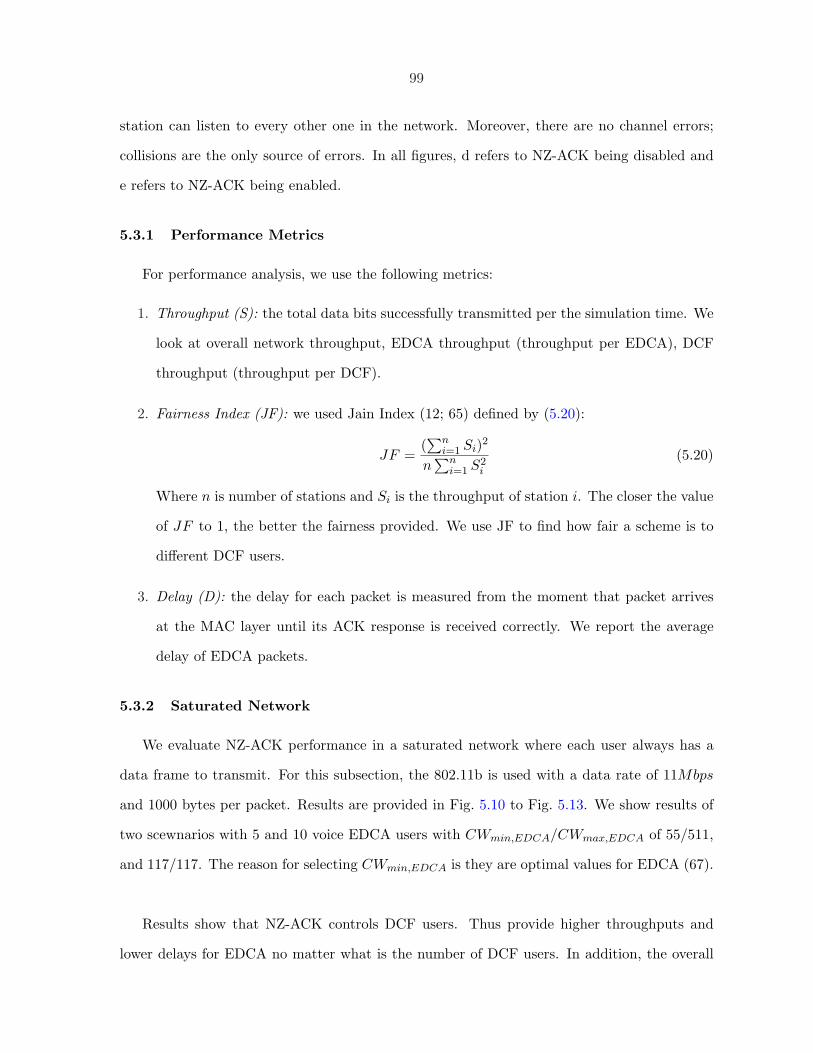
99
station can listen to every other one in the network. Moreover, there are no channel errors;
collisions are the only source of errors. In all figures, d refers to NZ-ACK being disabled and
e refers to NZ-ACK being enabled.
5.3.1 Performance Metrics
For performance analysis, we use the following metrics:
1. Throughput (S): the total data bits successfully transmitted per the simulation time. We
look at overall network throughput, EDCA throughput (throughput per EDCA), DCF
throughput (throughput per DCF).
2. Fairness Index (JF): we used Jain Index (12; 65) defined by (5.20):
JF =(∑n
i=1 Si)2
n∑n
i=1 S2i
(5.20)
Where n is number of stations and Si is the throughput of station i. The closer the value
of JF to 1, the better the fairness provided. We use JF to find how fair a scheme is to
different DCF users.
3. Delay (D): the delay for each packet is measured from the moment that packet arrives
at the MAC layer until its ACK response is received correctly. We report the average
delay of EDCA packets.
5.3.2 Saturated Network
We evaluate NZ-ACK performance in a saturated network where each user always has a
data frame to transmit. For this subsection, the 802.11b is used with a data rate of 11Mbps
and 1000 bytes per packet. Results are provided in Fig. 5.10 to Fig. 5.13. We show results of
two scewnarios with 5 and 10 voice EDCA users with CWmin,EDCA/CWmax,EDCA of 55/511,
and 117/117. The reason for selecting CWmin,EDCA is they are optimal values for EDCA (67).
Results show that NZ-ACK controls DCF users. Thus provide higher throughputs and
lower delays for EDCA no matter what is the number of DCF users. In addition, the overall

100
0
1
2
3
4
5
6
0 5 10 15 20 25 30 35
Number of DCF users
Th
rou
gh
pu
t M
bp
s
5 - S d 5 - S DCF d 5 - S EDCA d 5 - S e 5 - S DCF e 5 - S EDCA e
Figure 5.10 Throughput v.s. number of DCF users; 5 EDCA
0
1
2
3
4
5
6
0 5 10 15 20 25 30 35
Number of DCF users
Th
rou
gh
pu
t M
bp
s
10 - S d 10 - S DCF d 10 - S EDCA d
10 - S e 10 - S DCF e 10 - S EDCA e
Figure 5.11 Throughput v.s. number of DCF users; 10 EDCA
0
0.2
0.4
0.6
0.8
1
1.2
1.4
1.6
1.8
2
0 5 10 15 20 25 30 35
Number of DCF users
Del
ay s
eco
nd
s
5 - D EDCA d 5 - D EDCA e 10 - D EDCA d 10 - D EDCA e
Figure 5.12 Delay v.s. number of DCF users; 5,10 EDCA

101
0.94
0.95
0.96
0.97
0.98
0.99
1
1.01
0 5 10 15 20 25 30 35
Number of DCF usersF
I
5 - JF d 5 - JF e 10 - JF d 10 - JF e
Figure 5.13 Fairness Index v.s. number of DCF users
throughput performance of the network is enhanced. Also, the throughput DCF becomes
almost fixed when the number of DCF users gets very high. Actually, NZ-ACK first serve
EDCA users, and the remaining bandwidth is shared among DCF users. Finally, JF results
show that NZ-ACK lowers JF values as the number of DCF users increases. The reason is
that NZ-ACK reserves some time for EDCA users, and that time is not used by DCF users.
However, it is still considered fair enough as values of JF are always above 0.94.
5.3.3 Non-Saturated Network
Here, we evaluate the performance of 802.11 with NZ-ACK deployed in a non-saturated
network and compare it to that of 802.11 with no modification. We consider an 802.11b PHY
network with 11Mbps data rate, and CWmin/CWmax are 32/1024 (these are used by legacy
users). There are 15 voice EDCA users with CWmin/CWmax of 63/511. Each voice source is
modeled by an NO/OFF model with the ON and OFF periods are both exponential (0.352
seconds), and uses G.711 (silence) encoder with 64kbps coding rate and 160 bytes per one
packet. For legacy DCF users, number of users is varied. Each legacy user is saturated with
traffic of 1000 bytes per packet. DIFS of 50µs seconds is used by all users.
Fig. 5.14 shows the average total network throughput, average throughput per voice,
and average throughput per DCF users. Throughputs per voice are the same for NZ-ACK
and 802.11, which is also equivalent to the total voice load (not shown because it is the
same value). However, DCF throughput is slightly lowered with NZ-ACK enabled. Thus the

102
0
0.5
1
1.5
2
2.5
3
3.5
4
4.5
0 5 10 15 20 25 30 35
Number of DCF usersT
hro
ug
hp
ut
Mb
ps
S d S DCF d S EDCA d S e S DCF e S EDCA e
Figure 5.14 Throughput; 15 EDCA - on-off model
0
0.1
0.2
0.3
0.4
0.5
0.6
0.7
0.8
0.9
0 5 10 15 20 25 30 35
Number of DCF users
Del
ay s
eco
nd
s
D EDCA d D EDCA e
Figure 5.15 Delay; 15 EDCA - on-off model
total throughput is also slightly decreased (no change to EDCA throughput and lower DCF
throughput).
In Fig. 5.15, the packet delay for voice packets is illustrated. Results show that the delay
is maintained very small (a max value of 0.047761 seconds) for any number of DCF users
with NZ-ACK. The performance gain is due to the fact that NZ-ACK reduces the number
of contending users when issuing non-zero duration NZ-ACK frames; only EDCA users are
competing for the channel when DCF users are yielding.
5.4 Conclusions
The 802.11e standard is designed to be backward compatible with the 802.11. As a re-
sult, wireless networks are expected to have a combination of both EDCA (802.11e Enhanced
Distributed Channel Access) and legacy DCF (802.11 Distributed Control Function) users.

103
Typically, the 802.11e users who have QoS requirements are supposed to get a higher priority
service than that of legacy users. However, the EDCA users’ performance may be degraded
because of the existence of legacy users, and therefore would get a lower priority service. The
main reason for such effects is due to the fact that EDCA users are controlled through the use
of different contention parameters (AIFS, CWmin, CWmax, TXOP) that are distributed via
the beacon frames. In contrast, there is no control over legacy users because their contention
parameters (DIFS, CWmin, CWmax) are PHY dependent, i.e. they have constant values. As
a result, depending on the network status like the number of DCF/EDCA users, DCF users
could achieve a higher priority and could result in high collision rates, and thus degrade the
performance of EDCA users.
In this chapter, we discussed different aspects of the legacy DCF and EDCA coexistence
and provided general desirable features for any mitigation solution. Based on those features, we
proposed a simple distributed management scheme, called NZ-ACK, to mitigate the influence
of legacy DCF on EDCA performance in networks that consist of both types of users. NZ-ACK
controls legacy users by introducing a new ACK policy in which the QAP is allowed to set the
duration of the last ACK in a transmission exchange to a non-zero value.
In addition, we presented strategies to determine when to issue such NZ-ACK frames, and
the non-zero duration value of a NZ-ACK frame. NZ-ACK adapts to number of users, activity
or load level, and contention windows of both EDCA and DCF. All the processing of NZ-
ACK scheme is implemented at QAP. However, non-QAP EDCA users only are required to
distinguish the new ACK policy in order to ignore the non-zero value duration included in a
NZ-ACK frame. On the other hand, NZ-ACK requires no modification (i.e. fully transparent)
to legacy users. Thus, NZ-ACK maintains backward compatibility.
The proposed scheme allows EDCA users to start competing directly after NZ-ACK frames.
However, DCF users would defer their access to the channel according to the non-zero duration
of NZ-ACK frame. Moreover, when to issue NZ-ACK frames and their duration values are
determined adaptively according to network status. Thus, more resources for the EDCA users
are reserved in a dynamic and distributed fashion to maintain their priority. The performance
104
gain is due to the fact that NZ-ACK reduces the number of contending users when issuing
non-zero duration NZ-ACK frames; only EDCA users are competing for the channel when
DCF users are yielding. As a result, lower collision rates for both types of users are expected
and thus higher throughputs, and lower delays for EDCA.
Finally, we used Opnet Modeler to evaluate NZ-ACK and compare its performance to
that of IEEE 802.11. The results show that NZ-ACK outperforms IEEE 802.11 in terms of
maintaining the priority of service and delay bounds of EDCA users while providing acceptable
throughput for legacy users.

105
CHAPTER 6. Enhancing Bandwidth Utilization for the IEEE 802.16e
Submitted to the IEEE Transactions on Wireless Communications (TWC)
Haithem Al-Mefleh 1,3, J. Morris Chang 2,3
6.1 Abstract
The IEEE 802.16 provides a promising broadband wireless access technology, and thus
its efficiency is of high importance. We investigate encouraging ertPS (enhanced real time
Polling Service) connections to benefit from contention, and aims at improving the network
performance without violating any delay requirements of voice applications. Instead of always
allocating bandwidth to ertPS connections, we propose an algorithm that adaptively uses a
mix of contention and unicast polling. Moreover, as there is no differentiation between different
classes in contention in the current standard, a problem occurs when ertPS connections compete
with many BE (Best Effort) connections within a contention region. This would cause more
delays to get the required bandwidth of ertPS. Therefor, we also propose to implement a
mechanism at the SS’s scheduling side to maintain the priority of the delay-sensitive ertPS
connections in contention. We apply the new scheme to voice applications using the well-
known ON-OFF model. Finally, we use Qualnet Modeler for the performance evaluation.
Results show that the proposed scheme improves the jitter measures (with gains around 60%)
and the throughput performance (about 2% to 155% of gain) without violating any latency
requirements.1Graduate student.2Associate Professor.3Department of Electrical and Computer Engineering, Iowa State University.
106
6.2 Introduction
The IEEE 802.16 (37; 38) provides a promising broadband wireless access technology. Using
advanced communication technologies such as OFDM/OFDMA and MIMO, the IEEE 802.16 is
capable of supporting higher transmission rates, provides strong QoS mechanisms, and extends
the service ranges. Moreover, the IEEE 802.16 is evolving toward supporting nomadic and
mobile users (38), and using relay devices (68). Supported by these modern technologies,
WiMAX (Worldwide Inter-operability for Microwave Access) is able to provide a large service
coverage, a high speed data rate and QoS guaranteeing services. As a result, it may become
the last mile access in suburban areas replacing DSL and cable.
IEEE 802.16 defines both the MAC (medium access control) and PHY (physical) layers
of a broadband wireless network. The IEEE 802.16’s MAC is a connection-oriented reserva-
tion scheme in which the subscriber stations (SSs) have to reserve any required bandwidth
for transmissions. The BS (base station) coordinates reservations for all transmissions and
receptions. A connection is used to uniquely identify a flow from, or to, a SS. Hence, the stan-
dard also specifies bandwidth request/allocation mechanisms for different traffic service types.
Accordingly, efficient bandwidth requests, bandwidth allocations, scheduling at both BS and
SSs sides, QoS architectures, admission control, and traffic’s classifications are essential for
802.16 networks.
The IEEE 802.16 introduced different QoS classes which characterize different QoS require-
ments including UGS (Unsolicited Grant Services), rtPS (Real Time Polling Services), nrtPS
(Non Real Time Polling Services), and BE (Best Effort). The IEEE 802.16e-2005 added the
ertPS class as an enhancement for UGS and rtPS. Hence, it is expected that different real-
time applications will be using ertPS class instead of UGS and rtPS classes. Since UGS is
allocated unsolicited bandwidth and rtPS is polled periodically with higher priority, they are
not affected, and thus not considered, by our study. On the other hand, different applications
are using BE and nrtPS connections. For ertPS, the BS allocates bandwidth based on the
negotiated characteristics. However, when used for VBR (variable bit rate) applications, such
allocation may not be fully used due to the variability of traffic at a SS side. Hence, the total

107
efficiency or utilization of the network may be degraded.
In this chapter, we consider the performance of an IEEE 802.16 network with ertPS because
it is critical for VoIP applications. Thus, our work focuses on ertPS for voice applications using
the well-known ON-OFF model. Such model has proven to be practical and accurate. Our
main objective is to improve the network performance without violating the delay requirements
of voice applications. The improvement of throughput is due to the fact that the bandwidth
is allocated only when requested via bandwidth requests for an ertPS connection, and thus
the wasted bandwidth is much reduced and is given to other connections that actually need
it. Also, delay improvements is due to the proper use of unicast polling and the introduction
of service differentiation in contention.
Since the IEEE 802.16 allows ertPS to use both contention and unicast polling, we in-
vestigate encouraging ertPS connections to benefit from contention. Instead of always allo-
cating bandwidth to ertPS connections, we propose an algorithm that adaptively uses a mix
of contention and polling. However, as there is no differentiation between different classes in
contention in the current standard, a problem occurs when ertPS connections compete with
many low priority connections within a contention region. This would cause more collisions,
idle slots, and delays to get the required bandwidth. To overcome this problem, we propose
to implement a mechanism at the SS’s UL scheduler of bandwidth requests to maintain the
priority of the delay-sensitive ertPS connections in contention. While UGS connections are
granted bandwidth without any request, rtPS connections are polled periodically to request
bandwidth, and nrtPS connections are polled but less frequently than rtPS. On the other
hand, BE connections will be using contention most of the time as they are provided with
no guarantees. Hence, we consider the performance of ertPS and BE connections in an IEEE
802.16e network. Finally, we use Qualnet Modeler (69) for the performance evaluation. Re-
sults show that the proposed scheme improves the jitter measures (with gains around 60%)
and the throughput performance (about 2% to 155% of gain) without violating any latency
requirements.
The rest of the chapter is organized as following. First, section 6.3 gives an overview of

108
Frame n-1 Frame n Frame n+1
Preamble FCH DL burst 1 DL burst nContention Slots
for Initial Ranging
Contention Slots
for BW Requests
UL Burst
from SS 1
UL Burst
from SS n
Time
DL Subframe UL Subframe
TTG RTG
Figure 6.1 An example of IEEE 802.16 frame structure with TDD
IEEE 802.16 focussing on operations related to our work. Related work is discussed in section
6.4. Then, we illustrate the problem addressed, and we explain details of the proposed solution
in section 6.5. We also evaluate our work via Qualnet 4.5 simulation in section 6.6. Finally,
conclusions are provided in section 6.7.
6.3 An Overview of the IEEE 802.16 MAC
A reservation scheme is used in IEEE 802.16 networks to allow the SSs to reserve their
required bandwidth from the BS. In addition, IEEE 802.16 is connection-oriented. In other
words, the bandwidth requests are made based on the connection IDs (CID) which are used
for identifying the traffic flows between different SSs and the BS. Therefore, SSs must establish
connections with BS before transmitting any data. The BS can grant or reject the requests
based on the available bandwidth and scheduling policy.
There are two types of operational modes defined in the IEEE 802.16 standard: point-to-
multipoint (PMP) mode and mesh mode. An IEEE 802.16 PMP (point-to-multipoint) network,
which we consider in this chapter, includes a base station (BS) and a number of subscribers
(SSs) controlled by the BS. Also, there are two transmission modes: Time Division Duplex
(TDD) and Frequency Division Duplex (FDD). Both UL and DL transmissions can not be
operated simultaneously in TDD mode but in FDD mode. The time is divided into frames,
and each frame is divided into a DL (downlink) and an UP (uplink) subframes. DL subframe
is used for transmissions from the BS to SSs, and UL subframe is used for transmissions from
SSs to the BS. The BS controls the network by starting each frame with maps (UL MAP and
DL MAP) to indicate which and when SSs are transmitting or receiving. Fig. 6.1 shows an
109
overview of an 802.16’s frame structure operating in the Time Division Duplex (TDD) mode.
The preamble is used to synchronize the BS and SSs, and time gaps (TTG and RTG) are
used to give the BS and SSs enough time for the transition between transmitting and receiving
operations. In addition, SSTGs (subscriber station transition gaps) separate the transmissions
of the various SSs during the uplink subframe.
Consequently, the standard introduces different QoS classes which characterize different
connections:
1. Unsolicited Grant Services (UGS): a fixed amount of bandwidth is granted periodically.
This is proper for CBR (Constant Bit Rate) traffic.
2. Real Time Polling Services (rtPS): the SS must first request bandwidth, and the BS
provide a periodic bandwidth request opportunities. This is used for VBR (Variable Bit
Rate) with delay sensitivity characteristics.
3. Extended Real Time Polling Services (ertPS): a new class that was added by IEEE
802.16e to enhance the efficiency of UGS and rtPS.
4. Non Real Time Polling Services (nrtPS): like rtPS but for applications without delay
requirements.
5. Best Effort (BE): no guarantees are provided for best effort users.
In addition, the IEEE 802.16 standard defines different bandwidth request and allocation
schemes:
1. Unicast Polling: the BS allocates enough time in the UL for a SS to request bandwidth.
2. Piggybacking: a SSs can append the bandwidth request subheader to the regular MAC
header for requesting more bandwidth.
3. Bandwidth Stealing: If SSs grant the bandwidth for pervious bandwidth requests, they
can use the granted bandwidth to send another bandwidth request messages instead of
transmitting data.

110
4. Contention: SSs contend for the channel to send bandwidth requests using a backoff
procedure.
5. Unsolicited Grant: an amount of bandwidth is always granted for a connection without
any bandwidth request.
Table 6.1 summarizes the poll and grant options for each scheduling service according to the
IEEE 802.16/802.16e standards.
In this work, we consider the performance for SSs that are allowed to use both the
contention-based polling and the unicast polling. Contention-based polling (or simply con-
tention) follows a truncated exponential backoff procedure, and is controlled by start/end
backoff values and a number of the request transmission opportunities which are broadcast by
the BS. The SS transmits a bandwidth request when its backoff counter reaches zero. The
SS doubles its contention window and reattempt to send the bandwidth request if no grant
is received within a timeout value. Contention can be used only by BE, nrtPS, and ertPS
connections and has two types. Broadcast polling is where all SSs contend for the channel,
and multicast polling is where a group of SSs can participate in contention. On the other hand,
the BS allocates enough bandwidth for a SS to request bandwidth using unicast polling. Such
allocation simplifies the MAC operations, and provide delay guarantees. The BS provides pe-
riodic unicast polling for a connection with the period being determined using the negotiated
requirements at the setup time.
6.4 Related Work
Many studies of IEEE 802.16 have been conducted via simulation and analytical modeling.
These studies include the performance of different classes, optimization of contention parame-
ters, bandwidth requests and allocation, quality of service (QoS) architectures, scheduling, and
many other features of 802.16. An overview of IEEE 802.16 WiMAX is provided in (70; 71).
In the following, we summarize research work relevant to our work.
In (39), a simulation study is given for rtPS, nrtPs, and BE connections in the UL. Here,
it is shown that nrtPS and BE have almost the same performance, and rtPS outperforms

111
Tab
le6.
1Pol
l/gr
ant
opti
ons
for
each
sche
dulin
gse
rvic
e(3
7;38
)
Sche
dulin
gP
iggy
back
Ban
dwid
thU
nica
stpo
lling
Con
tent
ion-
base
dse
rvic
egr
ant
requ
est
stea
ling
polli
ng
UG
S-
Uns
olic
ited
Gra
ntSe
rvic
eN
otA
llow
edN
otA
llow
edPol
l-M
Ebi
tfo
rno
nU
GS
Not
allo
wed
ertP
S-
exte
nded
rtP
SE
xten
ded
pigg
ybac
kA
llow
edA
llow
edA
llow
edrt
PS
-R
ealT
ime
Pol
ling
Serv
ice
Allo
wed
Allo
wed
Allo
wed
Not
allo
wed
nrtP
S-
Non
Rea
lT
ime
Pol
ling
Serv
ice
Allo
wed
Allo
wed
Allo
wed
Allo
wed
BE
-B
est
Effo
rtA
llow
edA
llow
edA
llow
edA
llow
ed

112
nrtPS. It is also demonstrated that throughput decreases with a larger number of SSs due to
the overhead of preambles and headers of transmissions. It is also illustrated that the longer
the frame, the higher the average delay. Finally, it is shown that piggybacking is an efficient
mechanism, and can be done when there are multiple traffic sources in the same SS. In (40),
delay is analytically studied for three different simple polling schemes. However, the authors
assume that all SSs are polled sequentially in every UL subframe.
In WiMAX, scheduling and QoS architectures are essential to guarantee the demanded
QoS (41; 42; 43; 44). In general, scheduling and QoS architecture define the queues of data
and control packets, and how they are served (frequency, priority, and weight). In (44), for
example, UGS flows are served first. Then, rtPS and nrtPS connections are served with a
max-min allocation of bandwidth when there are no sufficient bandwidth. If any bandwidth
remains, it is given to BE connections in a round robin fashion.
The amount of bandwidth to allocate or to request is another interesting subject in 802.16
(45; 46; 47). In (45), a queue based scheduling scheme is used for rtPS and/or nrtPS connec-
tions. The allocated amount of bandwidth for a connection is based on number of packets in
the buffer of that connection. Then, a delay feedback is used to predict required bandwidth
during the next frame to prevent the buffer’s overflow. In (46), a similar approach is proposed
with two feedback parameters to calculate the bandwidth amount that should be requested. In
(47), simple formulas are used to find the amount of bandwidth allocated by the BS. The allo-
cated bandwidth is based on the connection parameters (like minimum bandwidth required),
amount of bandwidth requested, and the service type (like BE and ertPS). For example, a
UGS connection is always allocated all its required bandwidth without any request. Another
example is to allocate the needed time to send a bandwidth request message for an rtPS (or
ertPS) connection when its requested bandwidth is zero. However, this may degrade the per-
formance because of that allocated slots that are not used while they could have been assigned
to other SSs.
Contention operations are also studied for IEEE 802.16 (48; 49; 50; 51; 52; 53; 54; 55; 56; 57).
In (48), an optimal number of contentions slots is derived based on objective functions to reduce
113
the access delay. In (51), the start contention window is calculated in order to minimize
a cost function. In (50), the authors extended the Markov chain in (2) to model random
access in 802.16. Based on that model, an optimal fixed backoff window size is determined
to minimize the delay assuming a fixed number of active SSs. Performance analysis using a
Markov chain model for multicast and broadcast polling is provided in (55), and the ratio of
successfully transmitted requests is derived based on the given model. In (57), It is shown that
VoIP connections can have better performance when they are grouped into different multicast
groups. Unicast polling is also considered. For example, (72) provides an adaptive polling
scheme to increase the bandwidth utilization. Such adaptiveness would reduce the overhead
of polling a user with no data; i.e. a user who will waste the bandwidth given for polling. In
general, overheads include preambles, headers, unused bandwidth, and frequent signaling.
Different than other schemes, we utilize both polling and contention. In addition, we
propose to use a mechanism to differentiate different service types in contention, and thus
maintain the priority of delay-sensitive types while enhancing the network performance.
6.5 Details of the Proposed Solution
In this section, we first discuss the problem addressed. Then we provide details of the
proposed scheme including the algorithms proposed at the BS and SSs sides.
6.5.1 Problem Statement
The IEEE 802.16e-2005 added the ertPS class which allows for unsolicited grants like UGS
to save overheads of bandwidth requests. In addition, ertPS is allowed to dynamically adjust
the size of the bandwidth grant like rtPS to maximize the utilization. Moreover, ertPS is
allowed to use contentionbased polling to decrease the access delay and increase utilization. It
is expected that different real-time applications, like VoIP, will use ertPS class instead of rtPS
and UGS.
While UGS connections are granted bandwidth without any request, rtPS connections are
polled periodically to request bandwidth, and nrtPS connections are polled but less frequently

114
than rtPS. On the other hands, a large number of users are expected to use the BE class
specially when considering WEB users. Moreover, a significant number of BE users would
be using contention bandwidth requests most of the time since they are not guaranteed any
bandwidth. Consequently, we consider the performance of an IEEE 802.16 network with
ertPS and BE connections. The BS allocates bandwidth to ertPS connections based on the
negotiated characteristics. For VBR (variable bit rate) applications, such allocation may not
be fully used due to the variability of traffic at SSs side. Moreover, the unused bandwidth
allocated to ertPS connections can be used by other connections including ertPS and BE.
Hence, the performance of BE and ertPS connections, and the total efficiency or utilization of
the network may be degraded. For our study, we assume that the ertPS class is used for voice
applications with the well known ON-OFF model (an applicable model for voice and used by
many works. More information and references can be found in [24]). Finally, Qualnet Modeler
[26] will be used for the simulation study.
6.5.2 Description
The IEEE 802.16 allows ertPS to use both contention and unicast polls. Accordingly, we
summarize our proposal in the following:
1. The BS side: Instead of allocating data grants, or unicast polls, to ertPS connections,
we propose to have ertPS connections use contention while unicast polling them when
necessary, so SSs may request bandwidth. Therefore, we propose an algorithm at the
BS side to allocate bandwidth to ertPS connections to enhance the network performance
without violating the maximum latency requirements. Such algorithm allows dynamically
choosing the proper polling scheme, unicast polling or contention, for each SS depending
on the network conditions like the number of SSs of each class.
2. The SS side: A problem occurs when ertPS connections compete with many BE connec-
tions within a contention region due to the fact that there is no differentiation between
different classes in contention (all connections have the same start and end contention
windows, and follow the same backoff procedure) in the current standard. This would
115
cause more collisions, idle slots, and delays to get the required bandwidth. Thus, the
delay and throughput performance in the network may degrade. Accordingly, we need to
introduce a new mechanism to increase the priority of ertPS connections in contention.
In IEEE 802.16 standard, each SS has an UL scheduler for BW requests. Therefore, in
our scheme we propose that a SS schedules the start time of a bandwidth request of a BE
connection one contention slot after the beginning of the contention region. The reason
of using one slot is that it can be equivalent to doubling contention window (73), and
that more than one slot may result in starving BE connections. On the other hand, note
that there is no overhead added since no change is made to the UL map; i.e. no new
information is added to the UL map. Finally, pigyybacking should be used by a SS when
possible. Hence, the SS does not have to contend or wait for a unicast poll when more
data is available at the SS side.
6.5.3 Utilization
In the following, we assume that:
• N is the total number of SSs.
• tpoll is the polling period for a connection (negotiated at connection setup time).
• M is the size of contention region in number of transmission opportunities (slots).
• tf is the frame length.
• W is the initial contention window (W = 2S , S is the backoff start power value).
• T is a predefined period which is equal to an integer number of frames.
• nf represents a number of frames.
A simple way to find the utilization of polling and contention: Utilization = Total
Bandwidth − Wasted Bandwidth. In the following, we find the wasted bandwidth for polling
(Wp) and contention (Wc). For the traffic model for a connection at SSi, we are assuming

116
ON OFF ON OFF
An Arrival
Time
Figure 6.2 ON-OFF Model
an ON-OFF model (Fig. 6.2). The ON and OFF periods (i.e. TON , and TOFF ) are both
exponentially distributed with mean rates of α and β respectively. In addition, packets are
generated only during the ON period with a constant mean interarrival rate of λ. Tg represents
the interarrival time of packets.
TON ∼ Exp(α) (6.1)
TOFF ∼ Exp(β) (6.2)
Accordingly, the average ON time ton is 1α seconds, the average OFF time toff is 1
β seconds,
and the average interarrival time tg is 1λ seconds. We also define the ratio of ON time as ζ =
tonton+toff
, and the ratio of OFF time as η = toff
ton+toff.
A polling is wasted when it is not used to request bandwidth because no data exists at
the SS at the time of polling. The total ON time within a polling period can be estimated
by ζtpoll, and the OFF time within a polling period is ηtpoll. Then the probability that a SS
will make no bandwidth requests when polled can be found by calculating the probability of
having no data arrivals within tpoll. First, the probability of a SS having no data within one
ON period is:
P [TON <= tg] =∫ tg
0
1ton
et
ton dt
= 1− etg
ton (6.3)
hence, the probability the SS has data is ϕ=etg
ton . Then using tpoll
ton+toff , the average number
of ON periods within a tpoll, we approximate the probability that a SS has data within the
polling period using:

117
π = 1− (1− ϕ)ζtpollton
= 1− (1− ϕ)tpoll
ton+toff (6.4)
Thus, Nπ is the total number of SSs that are expected to have data. In other words, Wp=N(1−π) SSs are expected to waste their unicast polls.
Now we need to find an estimate of the bandwidth wastage in the contention scheme. The
waste in contention is simply the idle and collided slots. Since each user selects a backoff value
from the range [0,W − 1] using a uniform distribution, then we can find the probability that
a SS transmits in a slot (τ), the probability of a successful transmission in a slot (Ps), and the
probability of wasting a slot (υ).
τ =1W
(6.5)
We use the following can be used as a worst-case estimation (54).
Ps = N1W
(1− 1W
)N−1 (6.6)
υ = 1− Ps (6.7)
Consequently, the number of wasted slots can be defined as a binomial random variable X.
P [X = x] =
M
x
υx(1− υ)M−x (6.8)
Hence, the expected number of wasted slots is WC=υM .
6.5.4 Algorithm at BS
In this subsection, we provide details of the algorithm part to be run by the BS. In general,
the BS first allocates the data grants for ertPS connections. Then, we need to compensate for
contention. In other words, the algorithm maintains the probability of successful transmission

118
of BW requests in the contention region. Thereafter, the BS allocates unicast polls of a ertPS
connection if maximum delay requirement is to be violated. Finally, data grants of the low
priority BE connections are allocated. In the following, a detailed description of the algorithm
is provided.
The algorithm is summarized in Algorithm 1, and discussed in the following. In the algo-
rithm, the following terms are used:
• BWRi is the bandwidth requested by an ertPS connection.
• Ci is an an ertPS connection.
• Tc is current time.
• tf is the frame time.
• Ti is the last time a bandwidth request is received for Ci
• nertps is the number of ertPS connections
• nbe is the number of BE connections.
The algorithm is described in the following.
In lines 15 to 19 of Algorithm 1, the BS allocates a unicast poll for Ci (an ertPS connection)
in three conditions. First, when there is no bandwidth requested by that connection (BWRi
is 0). Second, if maximum latency requirement will be violated, or when (Tc+tf−Ti>=di).
Note that tf is added since the actual data grant occurs in the next frame. If a data grant
is allocated, then piggybacking is to be used by the corresponding SS, and thus the SS does
not have to contend or wait for a unicast poll in the subsequent frames. Finally, a unicast poll
is granted with a probability of π, i.e the probability the connection queue has some data to
transmit.
On the other hand, the utilization of contention region may be reduced since more connec-
tions are expected to compete. Therefore, as shown by line 3 to 14 of Algorithm 1, we need
to adjust contention when (na>1) where na refers to the number of ertPS connections who

119
are expected to contend for the channel. In other words, na represents the expected number
of active ertPS connections, and it is equivalent to nertpsπ. Starting from M and up to Mmax
(Mmax = W ), we find Mi that satisfies ((nbe +na) 1Mi
(1− 1Mi
)nbe+na−1 >= nbe1M (1− 1
M )nbe−1).
In other words, we find the first Mi value that maintains the utilization of contention consid-
ering the new number of contenders (nbe + na).
Algorithm 1 BS Side
1: Allocate data grants for ertPS2: na ⇐ bnertpsπc3: if na > 1 then4: ps ⇐ nbe
1M (1− 1
M )nbe−1
5: i ⇐ M
6: while i <= Mmax do7: pi ⇐ (nbe + na) 1
M (1− 1M )nbe+na−1
8: i ⇐ i + 19: if pi > ps then
10: break;11: end if12: end while13: M ⇐ i
14: end if15: for i = 1 to nertps do16: if BWRi == 0 AND Tc + tf − Ti >= dmax then17: Allocate a unicast polling for SSi with probability π
18: end if19: end for20: Allocate data grants for BE
6.6 Simulation
This section presents the simulation we used to evaluate the performance of the proposed
scheme. We utilized Qualnet 4.5 (69) to implement the new scheme by modifying the IEEE
802.16 model.
As shown in Fig. 6.3, we consider a network of IEEE 802.16 with one BS and a number
of SSs. In addition, each SS has one data traffic connection with a service type of BE or
ertPS. The main network parameters are stated in Table 6.2. Moreover, it is worth mentioning

120
BS
SS1
SSn
SSn+1
SSn+m
BE
ertPS
Figure 6.3 Network topology
that different main features of IEEE 802.16 are implemented including fragmentation, packing,
admission control, ranging, burst profiles, Adaptive Modulation and Coding (AMC), and CRC.
Each scheduler at the BS, or SS, follows a strict priority of different service types (management
> UGS > ertPS > rtPS > nrtPS > BE). In addition, the BS uses a WFQ scheduling for fairness
of each service type in the UL subframe. Finally, IP networking is used and nrtPS service type
is used for routing and transport layers. These connections have higher priority as they are
classified as management connections.
6.6.1 Traffic Characteristics
Each SS has one data connection which is a CBR or VoIP application which are provided
by Qualnet modeler. A CBR source is used for every BE connection, and a VoIP source is as-
sociated with each ertPS connection. Each VoIP source is modeled by an NO-OFF model with
the ON and OFF periods are both exponential with means of 0.352s and 0.648s, respectively.
In addition, the voice source uses silence encoder with a 160 bytes per voice packet, and each
voice packet is generated every 20ms only during the ON period. Also, the maximum latency
is set to 0.1s for each VoIP connection. On the other hand, a CBR application generates
packets with a constant rate of 0.0007s, and the data packet size is 1024 bytes. This allows an
almost saturated BE connections providing a high effect on ertPS connections.
6.6.2 Performance Metrics
For performance analysis, we use the following metrics:
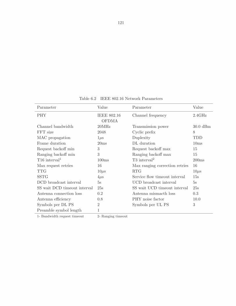
121
Table 6.2 IEEE 802.16 Network Parameters
Parameter Value Parameter Value
PHY IEEE 802.16 Channel frequency 2.4GHzOFDMA
Channel bandwidth 20MHz Transmission power 30.0 dBmFFT size 2048 Cyclic prefix 8MAC propagation 1µs Duplexity TDDFrame duration 20ms DL duration 10msRequest backoff min 3 Request backoff max 15Ranging backoff min 3 Ranging backoff max 15T16 interval1 100ms T3 interval2 200msMax request retries 16 Max ranging correction retries 16TTG 10µs RTG 10µsSSTG 4µs Service flow timeout interval 15sDCD broadcast interval 5s UCD broadcast interval 5sSS wait DCD timeout interval 25s SS wait UCD timeout interval 25sAntenna connection loss 0.2 Antenna mismacth loss 0.3Antenna efficiency 0.8 PHY noise factor 10.0Symbols per DL PS 2 Symbols per UL PS 3Preamble symbol length 11- Bandwidth request timeout 2- Ranging timeout

122
0
20000000
40000000
60000000
80000000
100000000
120000000
140000000
0 2 4 6 8 10 12
n
BE
Byte
s
1686500
1687000
1687500
1688000
1688500
1689000
1689500
ert
PS
Byte
s
BE - d BE - e ERTPS - d ERTPS - e
Figure 6.4 Throughput - 2 ertps SSs
1. Throughput: the throughput, in bytes, of both BE and ertPS connections.
2. Delay: the average end-to-end delay of ertPS connections in seconds.
3. Jitter: the average jitter, or delay variation, of ertPS connections in seconds.
6.6.3 Results
We start with a network where the number of ertPS connections is fixed, and the number
of BE SSs is variable. Then, we fix the number of BE connections and vary the number of
ertPS connections. In all figures presented, ”e” refers to the proposed scheme being enabled,
and ”d” represents the case where it is disabled.
6.6.3.1 2 ertPS connections
Here, the number of ertPS connections is set to 2, and n refers to number of BE connec-
tions. Figure 6.4 shows the throughput of BE and ertPS connections. As illustrated in these
figures, the throughput is enhanced for both types of services. While the gain is very small for
ertPS, it ranges from 5% to 16.19% for BE. With the proposed scheme, bandwidth is allocated
more efficiently. In other words, the new scheme reduces much of the wasted bandwidth, and
allocates such bandwidth to other connections that actually require it.
Figure 6.5 shows that the new scheme enhances the delay performances except for when n
= 4 (gain of −2%). In all other cases, the gain goes from 4% to 11% approximately. However,

123
0
0.01
0.02
0.03
0.04
0.05
0.06
0.07
0 2 4 6 8 10 12
n
Sec
on
ds
Delay - d Jitter - d Delay - e Jitter - e
Figure 6.5 Delay and jitter - 2 ertps SSs
the maximum latency is not violated in all cases, and delay is kept very small. Moreover, the
jitter performance is enhanced for all cases with gains up to around 60% as demonstrated in
figure 6.5. Delay requirement is met and jitter is improved because of the use of unicat polling
when the maximum latency is to be violated. In addition, an ertPS connection does not have
to wait for polling once it requires bandwidth, i.e. it would send a bandwidth request using
contention. Also, ertPS connections have a higher priority than that of BE connections in
contention because of the introduced service differentiation in our proposed scheme.
6.6.3.2 4 ertPS connections
In this experiment, we increase the number of ertPS connections by 2. The value of n
represents the number of BE connections. The throughput of BE and ertPS connections are
given in figure 6.6. There is still a very small improvement in ertPS throughput. On the other
hand, there is a higher gain for BE with a range of 6%−155%.
Figure 6.7 shows an improvement of delay for all values of n. The gain is from around 36%
to 44%. Again, the maximum latency is not violated, and delays are kept at low values. In
addition, the jitter gain is almost 63% as can be seen from figure 6.7.
Note that there is a higher gain than that of the pervious scenario of 2 ertPS in subsection
6.6.3.1. This is due to the increase of number of ertPS connections. In other words, more
bandwidth is better utilized with the proposed scheme.

124
0
20000000
40000000
60000000
80000000
100000000
120000000
140000000
160000000
180000000
0 2 4 6 8 10 12
n
BE
Byte
s
3373000
3374000
3375000
3376000
3377000
3378000
3379000
ert
PS
Byte
s
BE - d BE - e ERTPS - d ERTPS - e
Figure 6.6 Throughput - 4 ertps SSs
0
0.01
0.02
0.03
0.04
0.05
0.06
0.07
0 2 4 6 8 10 12
n
Sec
on
ds
Delay - d Jitter - d Delay - e Jitter - e
Figure 6.7 Delay ertps - 4 ertps SSs

125
0
20000000
40000000
60000000
80000000
100000000
120000000
140000000
0 2 4 6 8 10 12
n
BE
Byte
s
0
1000000
2000000
3000000
4000000
5000000
6000000
7000000
8000000
9000000
ert
PS
Byte
s
BE - d BE - e ERTPS - d ERTPS - e
Figure 6.8 Throughput BE - 4 BE SSs
0
0.01
0.02
0.03
0.04
0.05
0.06
0.07
0.08
0 2 4 6 8 10 12
n
Sec
on
ds
Delay - d Jitter - d Delay - e Jitter - e
Figure 6.9 Delay ertps - 4 BE SSs
6.6.3.3 4 BE connections
Finally, we set the number of BE connections to 4 and vary the number of ertPS connec-
tions. Here, n refers to the number of ertPS connections. The throughputs of BE and ertPS
connections are given in figure 6.8. While there is almost no difference in ertPS throughput,
gains of BE throughput goes from around 2% to 27%.
As explained by figure 6.9, delay results show gains in all cases with values from around
6% to 36%. In addition, the jitter performance is increased as can be inferred from figure 6.9.
Gains of jitter are about 60% to 63%.
As it can be seen from different results, the proposed scheme improves the throughput of the
network, the throughput of ertPS and BE connections, and thus does improve the utilization of
bandwidth allocation. The total throughput of the network is improved since both throughputs

126
of ertPS and BE connections are increased. The improvement of different throughputs is due
to the fact that the bandwidth is allocated only when requested via bandwidth requests for
the ertPS connections, and thus the wasted bandwidth is much reduced and is given to BE
connections that actually need it. In addition, the improvement occurs without violating the
maximum latency required by voice applications. Moreover, the jitter is much reduced, and
in almost all cases the delay is enhanced. Hence, the priority of ertPS is maintained due to
the differentiation used in contention. The results illustrate the effectiveness of the proposed
scheme as it adapts to different requirements and number of SSs.
6.7 Conclusions
The IEEE 802.16 provides a promising broadband wireless access technology, and is ex-
pected to replace or extend the already existing broadband communication technologies. There-
fore, the IEEE 802.16 efficiency is of high importance for academia and industry. We consider
voice applications using ertPS class that was introduced by the IEEE 802.16e-2005.
We investigated encouraging ertPS connections to benefit from contention to improve the
network performance without violating any delay requirements of voice applications. Instead of
always allocating bandwidth to ertPS connections, we proposed an algorithm that adaptively
uses a mix of contention and unicast polling. However, as there is no differentiation between
different classes in contention, a problem occurs when ertPS connections compete with many
BE connections as the collision rate increases within the contention region. As a result, there
would be more delays to get the required bandwidth of ertPS connections. Therefore, in our
scheme we propose that a SS schedules the start time of a bandwidth request of a BE connection
one contention slot after the beginning of the contention region. This would maintain the
priority of the delay-sensitive ertPS connections in the contention region. We also applied
the new scheme to voice applications using the well-known ON-OFF model. Finally, we used
Qualnet Modeler for the performance evaluation. Results showed that the proposed scheme
improves the jitter measures (with gains around 60%) and the throughput performance (about
2% to 155% of gain) without violating any latency requirements.
127
CHAPTER 7. Conclusions and Future Work
During the last few years, wireless networking has attracted much of the research and
industry interest. In addition, almost all current wireless devices are based on the IEEE
802.11 and IEEE 802.16 standards for the local and metropolitan area networks (LAN/MAN)
respectively. Both of these standards define the medium access control layer (MAC) and
physical layer (PHY) parts of a wireless user.
In a wireless network, the MAC protocol plays a significant role in determining the perfor-
mance of the whole network and individual users. Accordingly, many challenges are addressed
by research to improve the performance of MAC operations in IEEE 802.11 and IEEE 802.16
standards.
We proposed and studied solutions to enhance the performance of an IEEE 802.11 WLAN
and an IEEE 802.16 networks:
1. HDCF: The performance of 802.11 DCF degrades especially under larger network sizes,
and higher loads due to higher contention level resulting in more idle slots and higher
collision rates. We proposed HDCF to address the problem of wasted time in contention
resolution of DCF via classifying stations into active and inactive ones. The objectives
are to coordinate transmissions from different active stations with no collisions or idle
slots, and limit the contention to newly transmitting stations. HDCF utilizes an inter-
rupt scheme with active transmissions to enhance the fairness and eliminate, or reduce
much of, the costs of contention in DCF (idle slots and collisions) without adding any
assumptions or constraints to DCF.
We provided a simple analytical description of HDCF compared to DCF. We used a
simple but a well-known and an accurate model of the IEEE DCF which is presented

128
in (2), and we started with assumptions like that used in (2). We explained how new
arrivals affect the probability of collision, and how the collision level is reduced. We also
showed that like DCF, HDCF operation consists of cycles such that each cycle includes
on average a transmission by each user in the network. While DCF achieves this fairness
property with the cost of idle slots and collisions, HDCF reduces much of such overheads,
and thus is expected to enhance the throughput and fairness of the network.
In general, HDCF has the following advantages: 1) No idle slots wasted when there are
no new stations trying to transmit, or no need to stop active transmissions. 2) Fairness
to new stations as they can contend for the channel directly (like in DCF) without long
delays as the contention cost is much smaller. 3) Stations transmit in random order
without the need for a slotted channel, reserved periods, time synchronization, central
control, or knowledge of number of active users.
Finally, we used Opnet to provide a simulation study for networks of two different PHYs
(the IEEE 802.11b and 802.11g). In addition, the experiments considered different loads,
network sizes (number of users in the network), noise levels, packet sizes, and traffic
types. Results illustrated that HDCF outperforms DCF with gains up to 391.2% of
throughput and 26.8% of fairness level.
2. Taking Advantage of the Existence of Hidden Nodes: When wireless users are out of
range, they would not be able to hear frames transmitted by each other. This is referred
to as the hidden terminal problem, and significantly degrades the performance of the
IEEE 802.11 DCF because it results in higher collision rates.
Although the problem is addressed by different works, it is not totally eliminated. Hence,
we proposed a simple protocol that enhances the performance of DCF in the existence of
hidden terminal problem. Opposite to other approaches, we proposed to take advantage
of the hidden terminal problem whenever possible. We investigated if non-hidden stations
could help each other retransmit faster to enhance the performance of 802.11 WLANs.
Such cooperative retransmissions are expected to be faster since with DCF a non-collided

129
station mostly transmits earlier than collided stations that double their backoff values.
The proposed scheme modifies 802.11 DCF, is backward compatible, and works over the
802.11 PHY. We also presented an analysis model to calculate the saturation throughput
of the new scheme and compare it to that of DCF.
Capture effect is an advancement in wireless networks that allows a station to correctly
receive one of the collided frames under some conditions like a threshold of the received
signal’s SNR (signal-to-noise ratio). Thus, captures would enhance the throughout of the
network while decreasing the fairness level. Consequently, we considered capture effect as
it may reduce the gains of the proposed scheme, and would make it possible for the new
scheme to be used even in a fully-connected WLAN where there are no hidden nodes.
Using Opnet simulation, we evaluated the new scheme with and without the capture
effect for different topologies. Results showed gains of the number of retransmissions
per packet, throughput, fairness, delay, and packet drops. However, there was small
trade-off regarding fairness in some scenarios. Finally, simulation was used to validate
the analytical model.
3. NZ-ACK: The 802.11e standard is designed to be backward compatible with the 802.11.
Thus wireless networks are expected to have mix of EDCA (802.11e) and legacy DCF
(802.11, 802.11b, 802.11g, and 802.11a) users. As a result, EDCA users’ performance
may be degraded because of the existence of legacy users, and therefore would get a lower
priority of service. The main reason for such influence is due to the fact that EDCA users
are controlled through the use of different contention parameters, which are distributed
by a central controller. Nevertheless, there is no control over legacy users because their
contention parameters are PHY dependent, i.e. they have constant values.
We provided an insight on the effects of coexisting legacy DCF and EDCA devices,
and presented general desirable features for any proposed mitigating solution. Based
on these features, we then proposed a simple distributed scheme, called NZ-ACK (Non
Zero-Acknowledgement), to alleviate the influence of legacy DCF on EDCA performance

130
in networks consisting of both types of users.
NZ-ACK introduces a new ACK policy, and has the following features: 1) Simple and
distributed. 2) Fully transparent to legacy DCF users, and thus backward compatibility is
maintained. 3) No changes to the 802.11e standard frames formats. 4) Minimal overhead
to EDCA users as all processing is at the QAP. 5) Adaptively provide control over legacy
stations, and reserve more resources for the EDCA users as necessary.
Two variants of NZ-ACK were proposed. First, we used a simple intuition based on
number of users of both types and expected traffic at EDCA users. This variant requires
the AP to maintain virtual buffers for EDCA flows, and update these buffers depending
on admission information. Second, we provided a model for solving the main challenges
of NZ-ACK such that the priority of EDCA users is maintained. The model includes
contention parameters, the number of users, and transmission activities of both types of
users without the need for any virtual buffers or admission information.
Opnet simulation was used to evaluate both variants of NZ-ACK. Simulation results
showed that NZ-ACK maintains the priority of service and delay bounds of EDCA users
while providing acceptable throughput for legacy users.
4. Enhancing Bandwidth Utilization for the IEEE 802.16e: The IEEE 802.16 provides a
promising broadband wireless access technology, and is expected to replace or extend
the already existing broadband communication technologies. Therefore, the IEEE 802.16
efficiency is of high importance for academia and industry. We consider voice applications
using ertPS class that was introduced by the IEEE 802.16e.
We investigated encouraging ertPS connections to benefit from contention to improve
the network performance without violating any delay requirements of voice applications.
Instead of always allocating bandwidth to ertPS connections, we proposed that the BS
follows an algorithm that adaptively allocates contention or unicast polling for an ertPS
connection. Moreover, as there is no differentiation between different classes in con-
tention, a problem occurs when ertPS connections compete with low priority connections

131
connections within a contention region. This would cause more delays for an ertPS con-
nection to get its required bandwidth. Therefor, we proposed to implement a mechanism
at the SS’s UL scheduler of bandwidth requests to maintain the priority of the delay-
sensitive ertPS connections in the contention region. We also applied the new scheme to
VoIP applications using the well-known ON-OFF model. Finally, we used Qualnet Mod-
eler for the performance evaluation. Results showed that the proposed scheme improves
the jitter measures (with gains around 60%) for ertPS and the throughput performance
(about 2% to 155% of gain) without violating any latency requirements.
Future Work
In the following, we identify some open issues for future work:
1. HDCF was designed with the assumption of equal weights of different users. Thus, future
directions include extending HDCF to provide service differentiation among different
flows.
2. NZ-ACK was designed to maintain priority for high priority flows in EDCA when some
DCF users exist. Therefore, NZ-ACK can be redesigned to provide such priority among
different access categories in EDCA.
3. Due to the rich features of IEEE 802.16, different problems may need investigation. First,
allocation algorithms may consider a non-strict priority scheduling. Thus allowing higher
throughput for the low priority classes. Second, when allocating bandwidth, the BS may
consider the used data rate and energy level in addition to the class type of a connection.
Third, there is a need to consider different traffic types like video. Then, guidelines
may be provided to choose the right algorithm, or a generalized algorithm, for different
types. Fourt, channel errors and the use of ARQ (Automatic Repeat Request) may be
considered in the scheduling algorithm at BS.
132
BIBLIOGRAPHY
[1] Opnet, “Opnet Modeler.” http://www.opnet.com.
[2] G. Bianchi, “Performance analysis of the IEEE 802.11 distributed coordination function,”
Selected Areas in Communications, IEEE Journal on, no. 3, pp. 535–547, March 2000.
[3] IEEE Std 802.11b-1999, “Wireless LAN Medium Access Control (MAC) and Physical Layer
(PHY) Specifications: Higher-Speed Physical Layer Extension in the 2.4 GHz Band.”
[4] IEEE Std 802.11g-2003, “Part 11: Wireless LAN Medium Access Control (MAC) and
Physical Layer (PHY) specifications Amendment 4: Further Higher Data Rate Extension in
the 2.4 GHz Band.”
[5] Q. Ni, I. Aad, C. Barakat, and T. Turletti, “Modeling and analysis of slow cw decrease for
ieee 802.11 wlan,” 2003.
[6] Y. Kwon, Y. Fang, and H. Latchman, “A novel medium access control protocol with fast
collision resolution for wireless lans.” in INFOCOM, 2003.
[7] Z. G. Abichar and J. M. Chang, “Conti: Constant-time contention resolution for wlan
access.” in NETWORKING, 2005, pp. 358–369.
[8] C. Li and T. Lin, “Fixed Collision Rate Back-off Algorithm for Wireless Access Networks,”
in VTC Fall 2002, September 2002.
[9] L. Alonso, R. Ferrus, and R. Agusti, “Wlan throughput improvement via distributed queu-
ing mac,” Communications Letters, IEEE, vol. 9, no. 4, pp. 310–312, April 2005.

133
[10] I. Chlamtac, A. Farago, A.D. Myers, V.R. Syrotiuk, and G Zaruba, “Adapt: a dynamically
self-adjusting media access control protocol for ad hoc-networks,” Global Telecommunica-
tions Conference, 1999. GLOBECOM ’99, vol. 1A, pp. 11–15 vol.1a, 1999.
[11] J. L. Sobrinho and A. S. Krishnakumar, “Real-time Traffic over the IEEE 802.11 Medium
Access Control Layer,” Bell Labs Technical Journal, pp. 172–187, 1996.
[12] D. R. Jain, Chiu, and W. Hawe, “A Quantitative Measure of Fairness and Discrimina-
tion for Resource Allocation in Shared Computer Systems,” DEC Research Report TR-301,
September 1984.
[13] IEEE Std 802.11e-2005, “Part 11: Wireless LAN Medium Access Control (MAC) and
Physical Layer (PHY) specifications. Amendment 8: Medium Access Control (MAC) Quality
of Service Enhancements.”
[14] T. Athanasia and L. Dave, “Revisiting the hidden terminal problem in a csma/ca wireless
network,” Accepted for future publication in IEEE Transactions on Mobile Computing, 2007.
[15] H. Wu, F. Zhu, Q. Zhang, and Z. Niu, “Analysis of ieee 802.11 dcf with hidden terminals,”
in GLOBECOM. IEEE, 2006.
[16] S. Ray, D. Starobinski, and J. B. Carruthers, “Performance of wireless networks with
hidden nodes: a queuing-theoretic analysis,” Computer Communications, vol. 28, no. 10,
pp. 1179–1192, 2005.
[17] A. Zahedi and K. Pahlavan, “Natural hidden terminal and the performance of the wireless
lans,” Proc. IEEE 6th Int. Conf. on Univ. Pers. Comm., pp. 929–933, 1997.
[18] T. Nadeem, L. Ji, A. K. Agrawala, and J. R. Agre, “Location enhancement to ieee 802.11
dcf,” in INFOCOM. IEEE, 2005, pp. 651–663.
[19] M. Durvy, O. Dousse, and P. Thiran, “Modeling the 802.11 protocol under different
capture and sensing capabilities,” in INFOCOM. IEEE, 2007, pp. 2356–2360.
134
[20] L. Klienrock and F. Tobagi, “Packet switching in radio channels: Part i-carrier sense
multiple access modes and their throughput delay characteristics,” IEEE Transaction on
Communication, vol. COM-23, no. 12, pp. 1430–1416, Dec. 1975.
[21] J. Lee, W. Kim, S.-J. Lee, D. Jo, J. Ryu, T. Kwon, and Y. Choi, “An experimental
study on the capture effect in 802.11a networks,” WiNTECH’07, Montreal, Quebec, Canada,
September 10 2007.
[22] L. B. Jiang and S. C. Liew, “Hidden-node removal and its application in cellular wifi
networks,” IEEE Transactions on Vehicular Technology, vol. 56, no. 5, Part 1, pp. 2641–
2654, Sept. 2007.
[23] M. Borgo, A. Zanella, P. Bisaglia, and S. Merlin, “Analysis of the hidden terminal effect
in multi-rate ieee 802.11b networks,” September 2004.
[24] I. W.-H. Ho and S. C. Liew, “Impact of power control on performance of ieee 802.11
wireless networks,” IEEE Transactions on Mobile Computing, vol. 6, no. 11, pp. 1245 –
1258, Nov. 2007.
[25] D. Qiao, S. Choi, A. Jain, and K. Shin, “Adaptive transmit power control in ieee 802.11a
wireless lans,” Proc. of the IEEE Semiannual Vehicular Technology Conference 2003 (VTC
2003-Spring), vol. 1, pp. 433–437, April 2003.
[26] J. So and N. H. Vaidya, “Multi-channel mac for ad hoc networks: handling multi-channel
hidden terminals using a single transceiver,” in MobiHoc, J. Murai, C. E. Perkins, and
L. Tassiulas, Eds. ACM, 2004, pp. 222–233.
[27] L. Klienrock and F. Tobagi, “Packet switching in radio channels: Part 11-the hidden termi-
nal problem in carrier sense multiple access and the busy tone solution,” IEEE Transactions
on Communications, vol. COM-23, no. 12, pp. 1417–1433, Dec. 1975.
[28] Z. Haas and J. Deng, “Dual busy tone multiple access (DBTMA)-a multiple access control
scheme for ad hoc networks,” IEEE Transactions on Communications, vol. 50, no. 6, pp.
975 – 985, June 2002.
135
[29] V. Bharghavan, A. Demers, S. Shenker, and L. Zhang, “Macaw: A media access protocol
for wireless lans,” Proc. ACM SIGCOMM, London, UK, Oct. 1994.
[30] R. Gupta and J. Walrand, “Impatient backoff algorithm: Fairness in a distributed ad-hoc
mac,” ICC, 2007.
[31] A. Swaminathan and J. Martin, “Fairness issues in hybrid 802.11b/e networks,” in Con-
sumer Communications and Networking Conference, 3rd IEEE CCNC, vol. 1, 8-10 Jan 2006,
pp. 50–54.
[32] G. Bianchi, I. Tinnirello, and L. Scalia, “Understanding 802.11e contention-based pri-
oritization mechanisms and their coexistence with legacy 802.11 stations.” IEEE Network,
vol. 19, no. 4, pp. 28–34, 2005.
[33] J. Majkowski and F. C. Palacio, “Coexistence of ieee 802.11b and ieee 802.11e stations in
qos enabled wireless local area network.” in Wireless and Optical Communications, A. O.
Fapojuwo and B. Kaminska, Eds. IASTED/ACTA Press, 2006, pp. 102–106.
[34] ——, “Qos protection for ieee 802.11e in wlan with shared edca and dcf access.” in Com-
munication Systems and Networks, C. E. P. Salvador, Ed. IASTED/ACTA Press, 2006,
pp. 43–48.
[35] L. Vollero, A. Banchs, and G. Iannello, “Acks: a technique to reduce the impact of legacy
stations in 802.11e edca wlans,” in Communications Letters, IEEE, vol. 9, no. 4, April 2005,
pp. 346–348.
[36] A. Banchs, A. Azcorra, C. Garcia, and R. Cuevas, “Applications and challenges of the
802.11e edca mechanism: an experimental study.” IEEE Network, vol. 19, no. 4, pp. 52–58,
2005.
[37] IEEE Std 802.16-2004. “IEEE Standard for Local and Metropolitan Area Networks Part
16: Air Interface for Fixed Broadband Wireless Access Systems”, IEEE Std 802.16-2004
(Revision of IEEE Std 802.16-2001), 2004.

136
[38] IEEE Std 802.16e-2005. “IEEE Standard for Local and metropolitan area networks Part
16: Air Interface for Fixed and Mobile Broadband Wireless Access Systems Amendment 2:
Physical and Medium Access Control Layers for Combined Fixed and Mobile Operation in
Licensed Bands and Corrigendum 1”, IEEE Std 802.16e-2005 and IEEE Std 802.16-2004/Cor
1-2005 (Amendment and Corrigendum to IEEE Std 802.16-2004), 2006.
[39] C. Cicconetti, A. Erta, L. Lenzini, and E. Mingozzi, “Performance evaluation of the ieee
802.16 mac for qos support,” Mobile Computing, IEEE Transactions on, vol. 6, no. 1, pp.
26–38, Jan. 2007.
[40] R. Iyengar, P. Iyer, and B. Sikdar, “Analysis of 802.16 based last mile wireless networks,”
Global Telecommunications Conference, 2005. GLOBECOM ’05. IEEE, vol. 5, pp. 5 pp.–,
28 Nov.-2 Dec. 2005.
[41] M. Hawa and D. Petr, “Quality of service scheduling in cable and broadband wireless
access systems,” Quality of Service, 2002. Tenth IEEE International Workshop on, pp. 247–
255, 2002.
[42] H. Alavi, M. Mojdeh, and N. Yazdani, “A quality of service architecture for ieee 802.16
standards,” Communications, 2005 Asia-Pacific Conference on, pp. 249–253, 03-05 Oct.
2005.
[43] J. Sun, Y. Yao, and H. Zhu, “Quality of service scheduling for 802.16 broadband wireless
access systems,” Vehicular Technology Conference, 2006. VTC 2006-Spring. IEEE 63rd,
vol. 3, pp. 1221–1225, 7-10 May 2006.
[44] N. Ruangchaijatupon and Y. Ji, “Adaptive scheduling with fairness in ieee 802.16e net-
works,” Wireless Communications, Networking and Mobile Computing, 2007. WiCom 2007.
International Conference on, pp. 1976–1979, 21-25 Sept. 2007.
[45] K. R. Raghu, S. K. Bose, and M. Ma, “A queue based scheduling approach for wman with
adaptive augmentation,” in To appear in WCNC 2008.

137
[46] E.-C. Park, H. Kim, J.-Y. Kim, and H.-S. Kim, “Dynamic bandwidth request-allocation
algorithm for real-time services in ieee 802.16 broadband wireless access networks,” in To
appear in INFOCOM 2008.
[47] A. Sayenko, O. Alanen, J. Karhula, and T. Hamalainen, “Ensuring the qos requirements
in 802.16 scheduling,” in MSWiM ’06: Proceedings of the 9th ACM international symposium
on Modeling analysis and simulation of wireless and mobile systems. New York, NY, USA:
ACM, 2006, pp. 108–117.
[48] J. Zhou, Y. Yang, D. Pang, X. Jin, J. Shi, and Z. Li, “Contention region allocation
optimization in ieee 802.16 ofdma systems,” in MSWiM ’07: Proceedings of the 10th ACM
Symposium on Modeling, analysis, and simulation of wireless and mobile systems. New
York, NY, USA: ACM, 2007, pp. 197–200.
[49] I. Koo, S. Shin, and K. Kim, “Performance analysis of random access channel in ofdma
systems,” Systems Communications, 2005. Proceedings, pp. 128–133, 14-17 Aug. 2005.
[50] A. Vinel, Y. Zhang, M. Lott, and A. Tiurlikov, “Performance analysis of the random
access in ieee 802.16,” Personal, Indoor and Mobile Radio Communications, 2005. PIMRC
2005. IEEE 16th International Symposium on, vol. 3, pp. 1596–1600, 11-14 Sept. 2005.
[51] S.-M. Oh and J.-H. Kim, “The optimization of the collision resolution algorithm for broad-
band wireless access network,” Advanced Communication Technology, 2006. ICACT 2006.
The 8th International Conference, vol. 3, pp. 1944–1948, 20-22 Feb. 2006.
[52] R. Iyengar, V. Sharma, K. Kar, and B. Sikdar, “Analysis of contention-based multi-
channel wireless mac for point-to-multipoint networks,” in WOWMOM ’06: Proceedings
of the 2006 International Symposium on on World of Wireless, Mobile and Multimedia
Networks. Washington, DC, USA: IEEE Computer Society, 2006, pp. 453–455.
[53] J. He, K. Guild, K. Yang, and H.-H. Chen, “Modeling contention based bandwidth request
scheme for ieee 802.16 networks,” Communications Letters, IEEE, vol. 11, no. 8, pp. 689–
700, August 2007.

138
[54] A. Sayenko, O. Alanen, and T. Hamalainen, “On contention resolution parameters for the
ieee 802.16 base station,” Global Telecommunications Conference, 2007. GLOBECOM ’07.
IEEE, pp. 4957–4962, 26-30 Nov. 2007.
[55] L. Lin, W. Jia, and W. Lu, “Performance analysis of ieee 802.16 multicast and broadcast
polling based bandwidth request,” Wireless Communications and Networking Conference,
2007.WCNC 2007. IEEE, pp. 1854–1859, 11-15 March 2007.
[56] A. Sayenko, O. Alanen, and T. Hamalainen, “Adaptive contention resolution for voip
services in the ieee 802.16 networks,” World of Wireless, Mobile and Multimedia Networks,
2007. WoWMoM 2007. IEEE International Symposium on a, pp. 1–7, 18-21 June 2007.
[57] O. Alanen, “Multicast polling and efficient voip connections in ieee 802.16 networks,” in
MSWiM ’07: Proceedings of the 10th ACM Symposium on Modeling, analysis, and simula-
tion of wireless and mobile systems. New York, NY, USA: ACM, 2007, pp. 289–295.
[58] J. Bates, Optimizing Voice in ATM/IP Mobile Networks. McGraw-Hill, 2002.
[59] H. Al-Mefleh and J. M. Chang, “High performance distributed coordination function for
wireless lans,” in Networking, ser. Lecture Notes in Computer Science, A. Das, H. K. Pung,
F. B.-S. Lee, and L. W.-C. Wong, Eds., vol. 4982. Springer, 2008, pp. 812–823.
[60] H. Al-Mefleh and J. Chang, “A new ack policy to mitigate the effects of coexisting ieee
802.11/802.11e devices,” INFOCOM 2008. The 27th Conference on Computer Communica-
tions. IEEE, pp. 2056–2064, April 2008.
[61] H. Al-Mefleh and J. M. Chang, “Turning Hidden Nodes into Helper Nodes in IEEE 802.11
Wireless LAN Networks,” in Networking, ser. Lecture Notes in Computer Science, A. Das,
H. K. Pung, F. B.-S. Lee, and L. W.-C. Wong, Eds., vol. 4982. Springer, 2008, pp. 824–835.
[62] B. Sadeghi, V. Kanodia, A. Sabharwal, and E. Knightly, “Opportunistic media access for
multirate ad hoc networks,” , September 2002.

139
[63] J.-P. Sheu, C.-H. Liu, S.-L. Wu, and Y.-C. Tseng, “A priority mac protocol to support
real-time traffic in ad hoc networks.” Wireless Networks, vol. 10, no. 1, pp. 61–69, 2004.
[64] R. Lam, V. Leung, and H. Chan, “Polling-based protocols for packet voice transport
over IEEE 802.11 wireless local area networks,” IEEE Wireless Communications, no. 1, pp.
22–29, Feb 2006.
[65] C. Koksal, H. Kassab, and H. Balakrishnan, “An Analysis of Short-Term Fairness in
Wireless Media Access Protocols,” In Proc. of ACM SIGMETRICS, 2000.
[66] IEEE Std 802.11a-1999, “Part 11: Wireless LAN Medium Access Control (MAC) and
Physical Layer (PHY) specifications Amendment 1: High-speed Physical Layer in the 5
GHz band.”
[67] M. Heusse, F. Rousseau, R. Guillier, and A. Duda, “Idle sense: an optimal access method
for high throughput and fairness in rate diverse wireless lans,” in SIGCOMM, R. Guerin,
R. Govindan, and G. Minshall, Eds. ACM, 2005, pp. 121–132.
[68] IEEE 802.16j-06/026r4 edition, “Air interface for fixed and mobile broadband wireless
access systems: Multihop relay specification,” June 2007.
[69] Scalable Network Technologies (SNT), “QualNet Developer,” http://www.scalable-
networks.com/products/developer.php.
[70] A. Yarali, B. Mbula, and A. Tumula, “Wimax: A key to bridging the digital divide,”
SoutheastCon, 2007. Proceedings. IEEE, pp. 159–164, March 2007.
[71] A. Shankar and R. Hegde, “Wimax on the road to future,” Wireless, Mobile and Multi-
media Networks, 2008. IET International Conference on, pp. 275–278, Jan. 2008.
[72] C. Nie, M. Venkatachalam, and X. Yang, “Adaptive polling service for next-generation
ieee 802.16 wimax networks,” Global Telecommunications Conference, 2007. GLOBECOM
’07. IEEE, pp. 4754–4758, Nov. 2007.

140
[73] Y. Lin and V. Wong, “Saturation throughput of ieee 802.11e edca based on mean value
analysis,” Wireless Communications and Networking Conference, 2006. WCNC 2006. IEEE,
vol. 1, pp. 475–480, April 2006.