Design and Analysis of Clinical Study 4. Sample Size Determination

Dr. Tuan V. Nguyen

Garvan Institute of Medical Research

Sydney, Australia

Practical Difference vs Statistical Significance

Outcome Group A Group B

Improved 9 18

No improved 21 12

Total 30 30

% improved 30% 60%

Chi-square: 5.4; P < 0.05“Statistically significant”

Outcome Group A Group B

Improved 6 12

No improved 14 8

Total 20 20

% improved 30% 60%

Chi-square: 3.3; P > 0.05“Statistically insignificant”

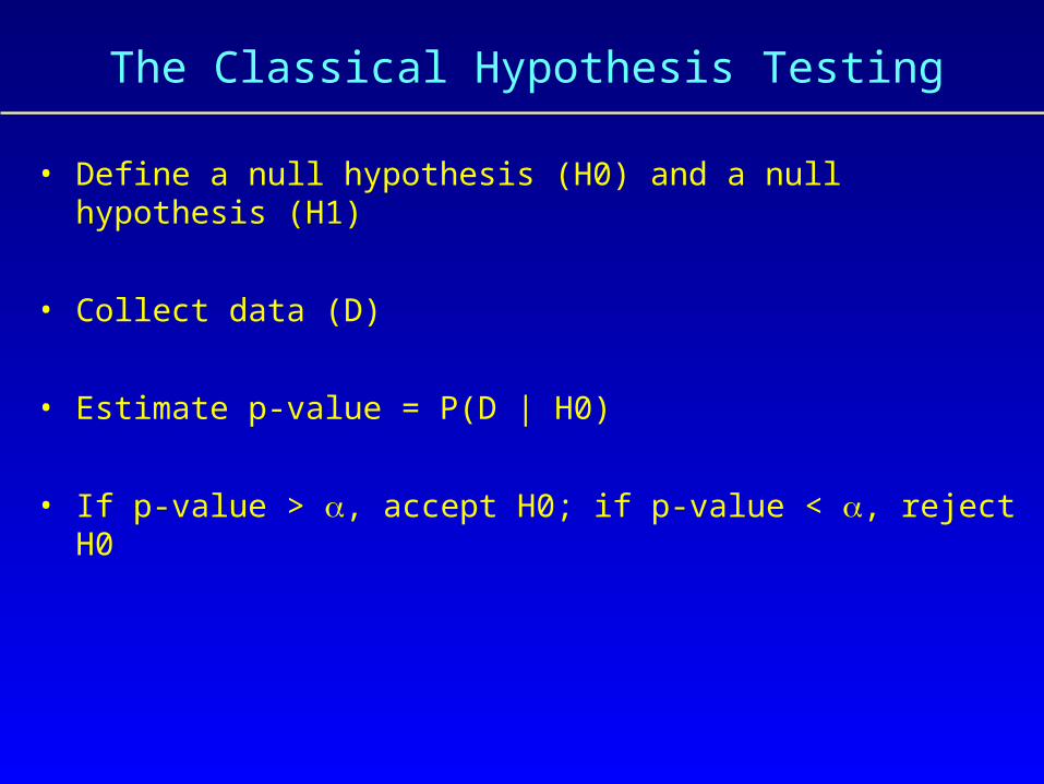
The Classical Hypothesis Testing

• Define a null hypothesis (H0) and a null hypothesis (H1)

• Collect data (D)

• Estimate p-value = P(D | H0)

• If p-value > , accept H0; if p-value < , reject H0

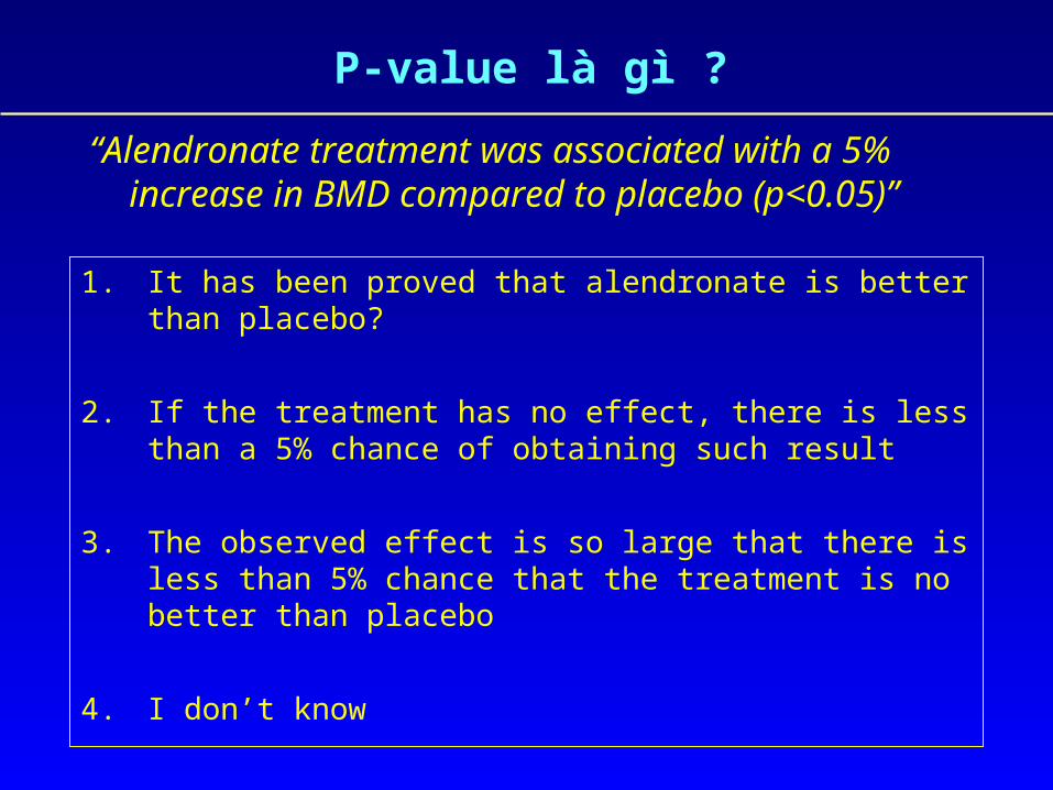
P-value là gì ?

“Alendronate treatment was associated with a 5% increase in BMD compared to placebo (p<0.05)”

1. It has been proved that alendronate is better than placebo?

2. If the treatment has no effect, there is less than a 5% chance of obtaining such result

3. The observed effect is so large that there is less than 5% chance that the treatment is no better than placebo

4. I don’t know

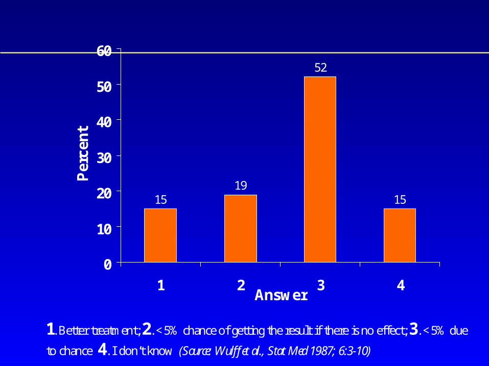
1519

52

15

0

10

20

30

40

50

60

1 2 3 4Answer

Per

cen

t

1. Better treatment; 2. <5% chance of getting the result if there is no effect; 3. <5% due

to chance 4. I don’t know (Source: Wulffet al., Stat Med 1987; 6:3-10)

P value is NOT

• the likelihood that findings are due to chance

• the probability that the null hypothesis is true given the data

• P-value is 0.05, so there is 95% chance that a real difference exists

• With low p-value (p < 0.001) the finding must be true

• The lower p-value, the stronger the evidence for an effect

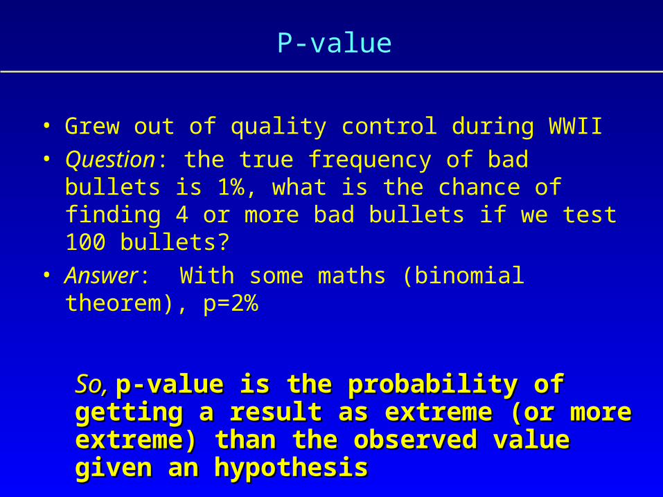
P-value

• Grew out of quality control during WWII • Question: the true frequency of bad bullets is 1%, what

is the chance of finding 4 or more bad bullets if we test 100 bullets?

• Answer: With some maths (binomial theorem), p=2%

So, So, p-value is the probability of getting p-value is the probability of getting a result as extreme (or more extreme) a result as extreme (or more extreme) than the observed value given an than the observed value given an hypothesishypothesis

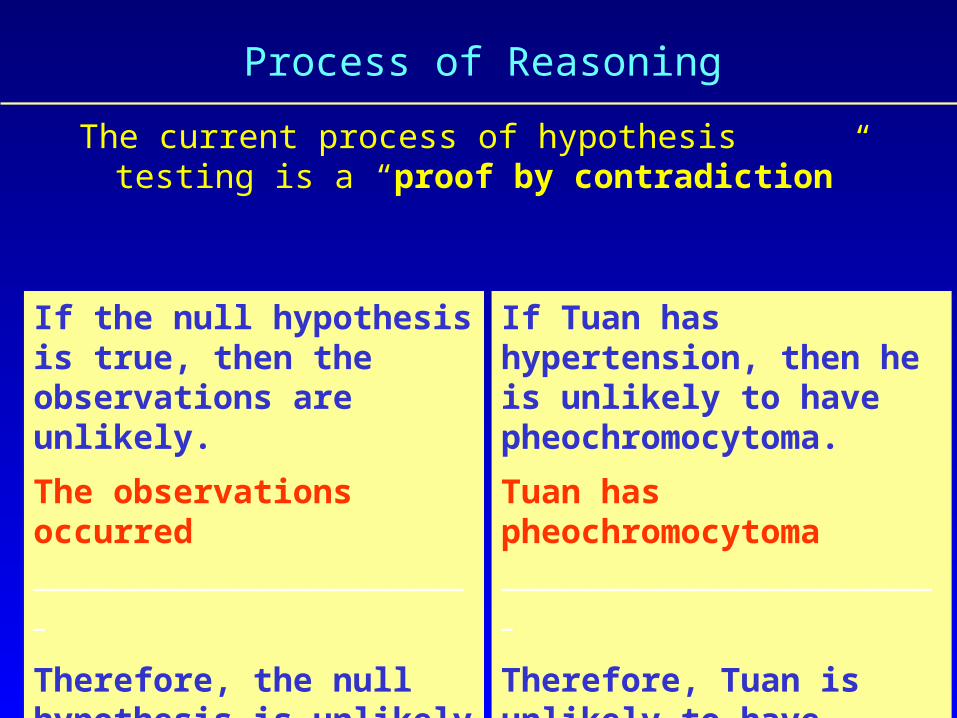
Process of Reasoning

The current process of hypothesis testing is a “proof by contradiction”

If the null hypothesis is true, then the observations are unlikely.

The observations occurred______________________________________

Therefore, the null hypothesis is unlikely

If Tuan has hypertension, then he is unlikely to have pheochromocytoma.

Tuan has pheochromocytoma______________________________________

Therefore, Tuan is unlikely to have hypertension

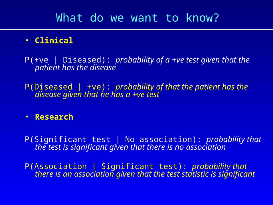
What do we want to know?

• Clinical

P(+ve | Diseased): probability of a +ve test given that the patient has the disease

P(Diseased | +ve): probability of that the patient has the disease given that he has a +ve test

• Research

P(Significant test | No association): probability that the test is significant given that there is no association

P(Association | Significant test): probability that there is an association given that the test statistic is significant

Diagnostic and statistical reasoning

Diagnosis Research

Absence of disease There is no real difference

Presence of disease There is a difference

Positive test result Statistical significance

Negative test result Statistical non-significance

Sensitivity (true positive rate) Power (1-)

False positive rate P-value

Prior probability of disease (prevalence)

Prior probability of research hypothesis

Positive predictive value Bayesian probability

Case study

• Một phụ nữ 45 tuổi• Không có tiền sử ung thư vú trong gia đình• Đi xét nghiệm truy tầm ung thư bằng mammography• Kết quả dương tính• Hỏi: Xác suất người phụ nữ này bị ung thư là bao nhiêu?

Các yếu tố liên quan cần biết để có câu trả lời:

- Tần suất ung thư trong quần thể

- Độ nhạy của test chẩn đoán

- Độ đặc hiệu của test chẩn đoán

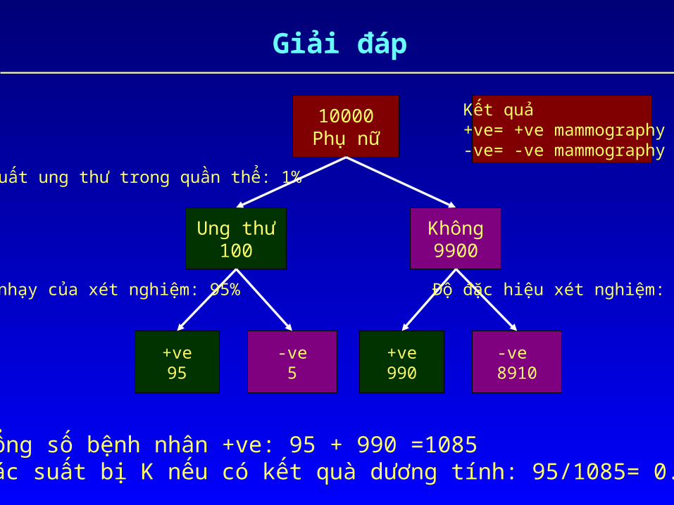
10000Phụ nữ

Ung thư100

Không9900

+ve95

-ve5

+ve990

-ve 8910

Tần suất ung thư trong quần thể: 1%

Độ nhạy của xét nghiệm: 95% Độ đặc hiệu xét nghiệm: 90%

Tổng số bệnh nhân +ve: 95 + 990 =1085Xác suất bị K nếu có kết quà dương tính: 95/1085= 0.087

Kết quả+ve= +ve mammography-ve= -ve mammography

Giải đáp

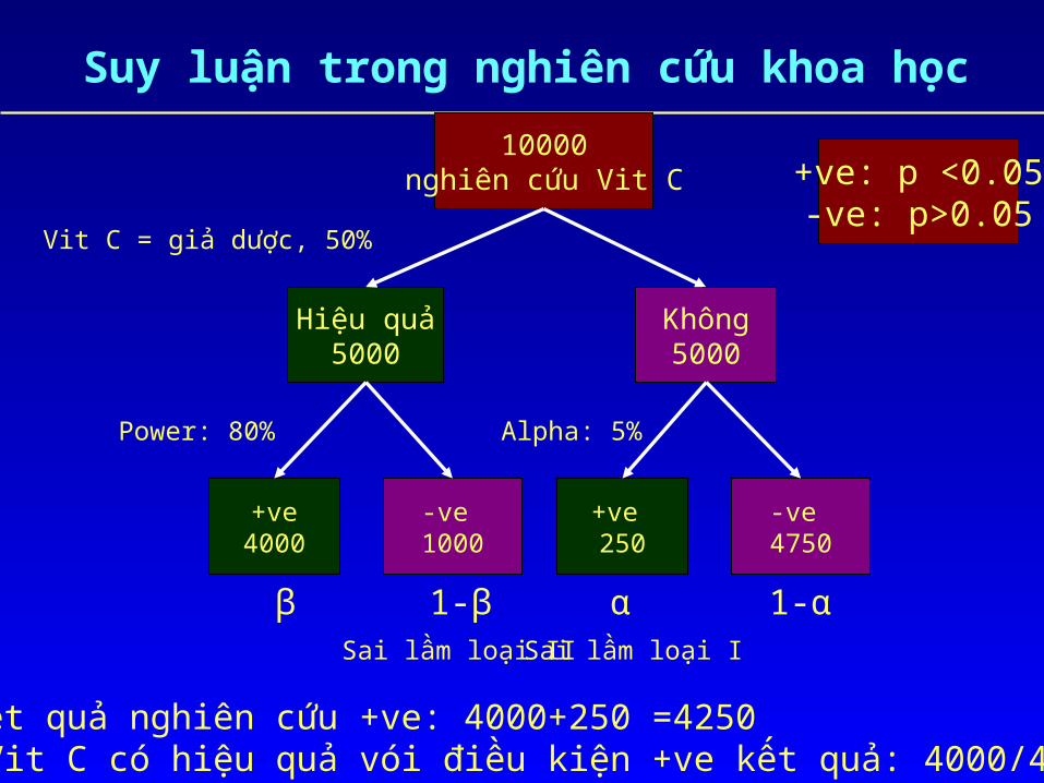
10000nghiên cứu Vit C

Hiệu quả5000

Không5000

+ve4000

-ve 1000

+ve 250

-ve 4750

Vit C = giả dược, 50%

Power: 80% Alpha: 5%

Tổng số kết quả nghiên cứu +ve: 4000+250 =4250Xác suất Vit C có hiệu quả vói điều kiện +ve kết quả: 4000/4250= 0.94

β α1-β 1-αSai lầm loại II Sai lầm loại I

+ve: p <0.05-ve: p>0.05

Suy luận trong nghiên cứu khoa học

What Are Required for Sample Size Estimation?

• Parameter (or outcome) of major interest– Blood pressure

• Magnitude of difference in the parameter– 10 mmHg is an important difference / effect

• Variability of the parameter– Standard deviation of blood pressure

• Bound of errors (type I and type II error rates)– Type I error = 5%– Type II error = 20% (or power = 80%)

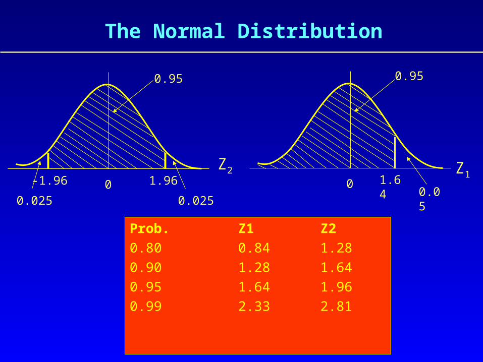
The Normal Distribution

0.95

0.025 0.0250-1.96 1.96

0.95

0.050 1.64

Prob. Z1 Z2

0.80 0.84 1.28

0.90 1.28 1.64

0.95 1.64 1.96

0.99 2.33 2.81

Z1Z2

The Normal Deviates

Alpha Z

c0.20 1.280.10 1.640.05 1.960.01 2.81

Power Z0.80 0.84

0.90 1.28

0.95 1.64

0.99 2.33

Study Design and Outcome

• Single population• Two populations

• Continuous measurement• Categorical outcome• Correlation

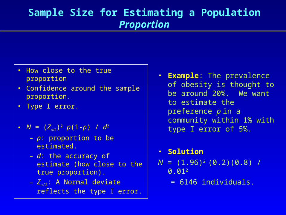
Sample Size for Estimating a Population Proportion

• How close to the true proportion• Confidence around the sample

proportion.• Type I error.

• N = (Z)2 p(1-p) / d2

– p: proportion to be estimated.– d: the accuracy of estimate

(how close to the true proportion).

– Z/2: A Normal deviate reflects the type I error.

• Example: The prevalence of obesity is thought to be around 20%. We want to estimate the preference p in a community within 1% with type I error of 5%.

• Solution

N = (1.96)2 (0.2)(0.8) / 0.012

= 6146 individuals.

Effect of Accuracy

• Example: The prevalence of disease in the general population is around 30%. We want to estimate the prevalence p in a community within 2% with 95% confidence interval.

• N = (1.96)2 (0.3)(0.7) / 0.022 = 2017 subjects.

0

500

1000

1500

2000

2500

0 0.02 0.04 0.06 0.08 0.1

Standard deviation

Sam

ple

size

Sample Size for Difference between Two Means

2

22

11

rd

ZZrN

• Hypotheses:Ho: m1 = m2 vs. Ha: m1 = m2 + d

• Let n1 and n2 be the sample sizes for group 1 and 2, respectively; N = n1 + n2 ; r = n1 / n2 ; s: standard deviation of the variable of interest.

• Then, the total sample size is given by:

• If we let Z = d/be the “effect size”then:

2

2

11

rZ

ZZrN

Where Z and Z1- are Normal deviates

• If n1 = n2 , power = 0.80, alpha = 0.05, then (Z + Z1-)2 = (1.96 + 1.28)2 = 10.5, then the equation is reduced to:

221

ZN

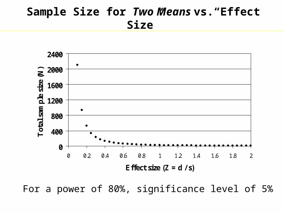
Sample Size for Two Means vs.“Effect Size”

0

400

800

1200

1600

2000

2400

0 0.2 0.4 0.6 0.8 1 1.2 1.4 1.6 1.8 2

Effect size (Z = d / s)

Tot

al s

ampl

e si

ze (

N)

For a power of 80%, significance level of 5%

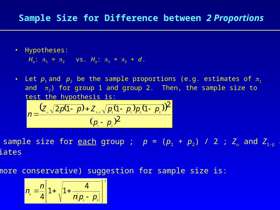
Sample Size for Difference between 2 Proportions

2

21112

21

22111

pp

ppppZppZn

• Hypotheses:Ho: 1 = 2 vs. Ha: 1 = 2 + d .

• Let p1 and p2 be the sample proportions (e.g. estimates of 1 and 2) for group 1 and group 2. Then, the sample size to test the hypothesis is:

Where: n = sample size for each group ; p = (p1 + p2) / 2 ; Z and Z1- are Normal deviates

A better (more conservative) suggestion for sample size is:2

21

411

4

ppn

nn

a

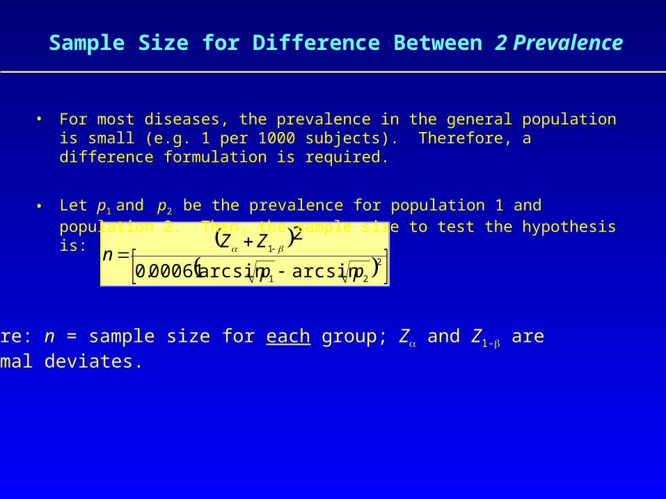
Sample Size for Difference Between 2 Prevalence

2

21

1

arcsinarcsin00061.0

2

pp

ZZn

• For most diseases, the prevalence in the general population is small (e.g. 1 per 1000 subjects). Therefore, a difference formulation is required.

• Let p1 and p2 be the prevalence for population 1 and population 2. Then, the sample size to test the hypothesis is:

Where: n = sample size for each group; Z and Z1- are Normal deviates.

Sample Size for Two Proportions: Example

• Example: The preference for product A is expected to be 70%, and for product B 60%. A study is planned to show the difference at the significance level of 1% and power of 90%.

• The sample size can be calculated as follows:

– p1 = 0.6; p2 = 0.7; p = (0.6 + 0.7)/2 = 0.65; Z = 2.81; Z = 1.28.

– The sample size required for each group should be:

75927.06.0

23.07.04.06.028.135.065.0281.2

n

• Adjusted / conservative sample size is:

8367.06.0759

411

4

7592

a

n

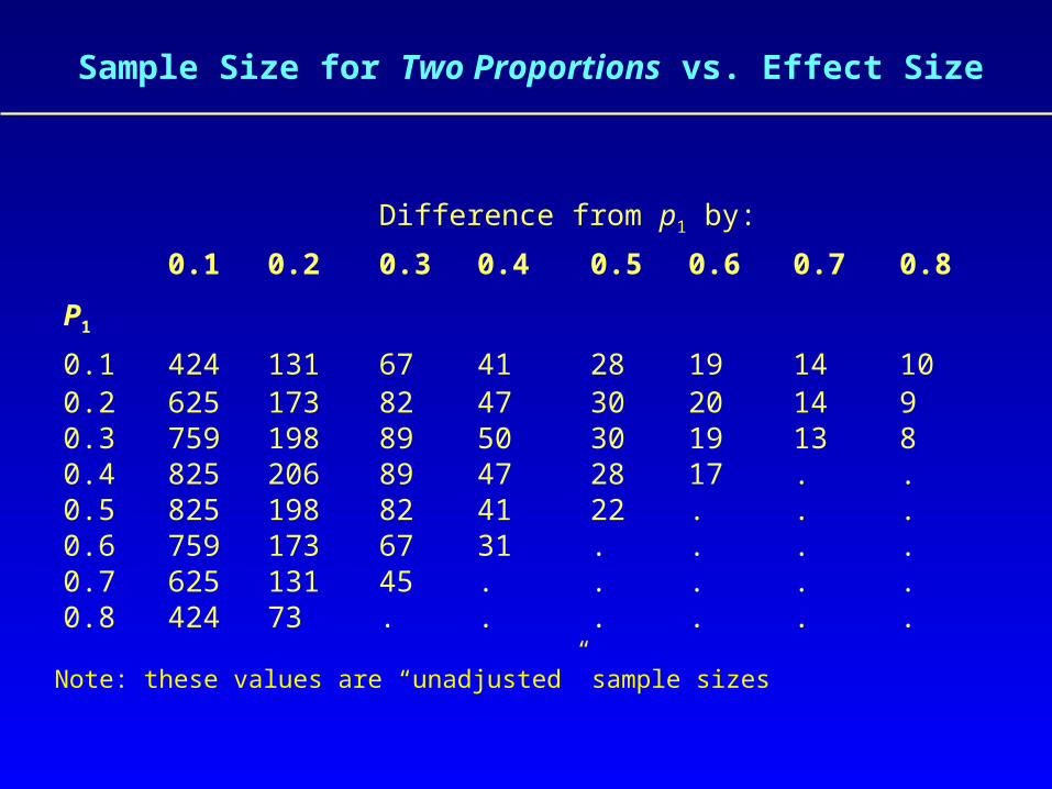
Sample Size for Two Proportions vs. Effect Size

Difference from p1 by:

0.1 0.2 0.3 0.4 0.5 0.6 0.7 0.8

P1

0.1 424 131 67 41 28 19 14 100.2 625 173 82 47 30 20 14 90.3 759 198 89 50 30 19 13 80.4 825 206 89 47 28 17 . .0.5 825 198 82 41 22 . . .0.6 759 173 67 31 . . . .0.7 625 131 45 . . . . .0.8 424 73 . . . . . .

Note: these values are “unadjusted” sample sizes

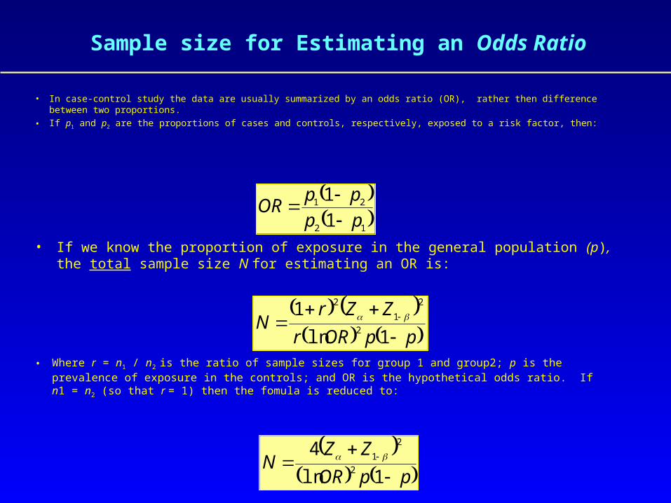
Sample size for Estimating an Odds Ratio

ppORr

ZZrN

1ln

12

2

1

2

• In case-control study the data are usually summarized by an odds ratio (OR), rather then difference between two proportions.

• If p1 and p2 are the proportions of cases and controls, respectively, exposed to a risk factor, then:

12

21

1

1

pp

ppOR

• If we know the proportion of exposure in the general population (p), the total sample size N for estimating an OR is:

• Where r = n1 / n2 is the ratio of sample sizes for group 1 and group2; p is the prevalence of exposure in the controls; and OR is the hypothetical odds ratio. If n1 = n2 (so that r = 1) then the fomula is reduced to:

ppOR

ZZN

1ln

42

2

1

Sample Size for an Odds Ratio: Example

• Example: The prevalence of vertebral fracture in a population is 25%. It is interested to estimate the effect of smoking on the fracture, with an odds ratio of 2, at the significance level of 5% (one-sided test) and power of 80%.

• The total sample size for the study can be estimated by:

27575.025.02ln

85.064.142

2

N

Some Comments

• The formulae presented are theoretical.• They are all based on the assumption of Normal distribution.• The estimator [of sample size] has its own variability.• The calculated sample size is only an approximation.• Non-response must be allowed for in the calculation.

Computer Programs

• Software program for sample size and power evaluation– PS (Power and Sample size), from Vanderbilt Medical Center. This can be

obtained from me by sending email to (t.nguyen@garvan.org.au). Free. • On-line calculator:

– http://ebook.stat.ucla.edu/calculators/powercalc/• References:

– Florey CD. Sample size for beginners. BMJ 1993 May 1;306(6886):1181-4– Day SJ, Graham DF. Sample size and power for comparing two or more treatment groups in

clinical trials. BMJ 1989 Sep 9;299(6700):663-5.– Miller DK, Homan SM. Graphical aid for determining power of clinical trials involving two

groups. BMJ 1988 Sep 10;297(6649):672-6– Campbell MJ, Julious SA, Altman DG. Estimating sample sizes for binary, ordered

categorical, and continuous outcomes in two group comparisons. BMJ 1995 Oct 28;311(7013):1145-8.

– Sahai H, Khurshid A. Formulae and tables for the determination of sample sizes and power in clinical trials for testing differences in proportions for the two-sample design: a review. Stat Med 1996 Jan 15;15(1):1-21.

– Kieser M, Hauschke D. Approximate sample sizes for testing hypotheses about the ratio and difference of two means. J Biopharm Stat 1999 Nov;9(4):641-50.