design &analysis of dna microarray studies · • experiment descriptor worksheet – rows...
TRANSCRIPT

Design &Analysis of DNA Design &Analysis of DNA Microarray Studies With BRBMicroarray Studies With BRB--
ArrayToolsArrayTools
Dr. Richard Simon [email protected]
http://linus.nci.nih.gov/brb

http://linus.nci.nih.gov/brb
• http://linus.nci.nih.gov/brb– Powerpoint presentations– Reprints & Technical Reports– BRB-ArrayTools software– BRB-ArrayTools Data Archive– Sample Size Planning for Targeted Clinical
Trials

Challenges in Effective Use of DNA Microarray Technology
• Design & Analysis are bigger challenges than data management. – Much greater opportunity for misleading yourselves and
others than traditional single gene/protein studies • Limited availability of experienced statistical
collaborators• Predominance of hype, mis-information, and
dangerous methods promulgated by biomedical scientists as well as professional statistical/computational scientists
• Predominance of flashy software that encourages misleading analyses
Objectives of BRB-ArrayTools
• Provide biomedical scientists access to statistical expertise for the analysis of expression data– training in analysis of high dimensional data – access to critical assessment of methods
published in a rapidly expanding literature

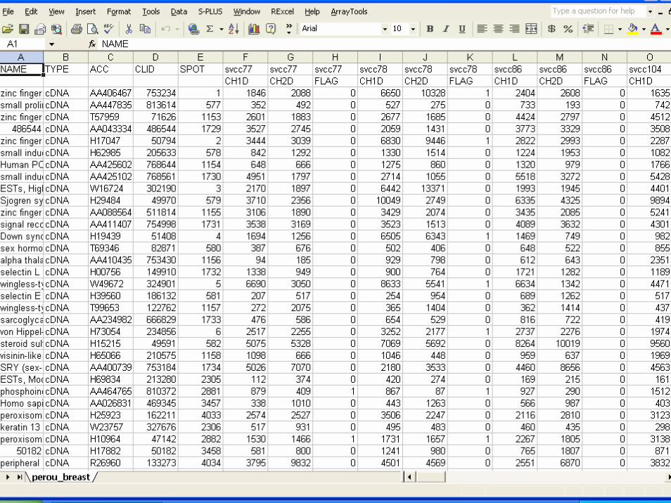
BRB-ArrayTools• Integrated package• Excel-based user interface
– Doesn’t use Excel analyses– state-of-the art analysis methods programmed in R, Java & Fortran– Data not stored as worksheets
• >1000 arrays and 65000 genes per project
• Based on continuing evaluation of validity and usefulness of published methods– Methods carefully selected by R Simon– Not a repository like Bioconductor
• Publicly available for non-commercial uses from BRB website:
BRB-ArrayTools• Not tied to any database
– Importer for common databases and platforms• MadB, GenePix, Agilent, MAS5/GCOS• Imports .cel files• Import wizzard for any files output by image analysis program
– Import (collate)• Expression data (eg separate file for each array)• Spot (probeset) identifiers• Experiment descriptor worksheet
– Rows correspond to arrays– Columns are user defined phenotypes to drive the analyses
» Can be updated during analysis– Imported data saved as project folder containing project workbook and
binary files• Project workbook can be re-opened in Excel at any time• Output saved in html files in output folder
BRB-ArrayTools
• Highly computationally efficient– Non-intensive analyses in R– Intensive analyses in FORTRAN
• eg BRB-AT version of SAM is 9x + more efficient than Bioconductor or web based versions
– And more accurate
• Extensive gene and pathway annotation features

BRB-ArrayTools
• Plug-in facility for user written R functions• Message board and listserve• Extensive built-in help facilities, tutorials,
datasets, usersguide, data import and analysis wizzards, sample statistical analysis sections, …
BRB-ArrayTools Archive of Human Tumor Expression Data
• http://linus.nci.nih.gov/brb/DataArchive.html• Archive of BRB-ArrayTools zipped project
folders of expression profiles of human tumors and associated clinical/pathological descriptors– Published data
• Easy way to archive your data and to analyze someone else’s data– Download, unzip, open in Excel

• Design and Analysis of DNA Microarray Investigations– R Simon, EL Korn, MD Radmacher, L McShane, G
Wright, Y Zhao. Springer (2003)

Brief Review of Microarray Technology
Microarray Expression Profiling
• Would like to know the concentration of each protein in a cell– Proteins do the work of cells– Proteins have many shapes and parallel assays
for all proteins have not been developed
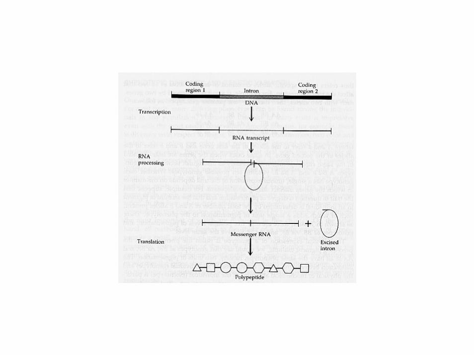
Microarray Expression Profiling
• One gene transcription produces one mRNA molecule produces one protein molecule
• # genes ≅ # mRNA types• mRNA molecule can be reverse transcribed into
DNA and will bind only to the gene from which it was originally transcribed (to which it is homologous)

Microarray Expression Profiling
• Estimates abundance of mRNA molecules of each type present in cells– Assay not sensitive enough to analyze single
cells so estimate is for average of sample of cells
• Microarray contains a spot of DNA corresponding to each gene– Spots are in known fixed positions– Spots contain fewer nucleotides that the full
gene

Gene Expression Microarrays
• Permit simultaneous evaluation of expression levels of thousands of genes
• Main platforms– cDNA printed on glass slides– Externally synthesized oligos printed on glass slides – Affymetrix GeneChips– Oligos in-situ synthesized on glass slides– cDNA printed on nylon filters
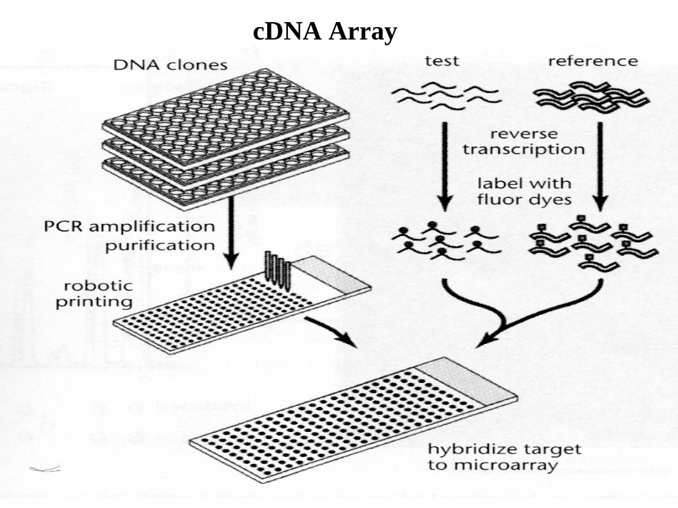
cDNA Array


cDNA & Printed Oligo Arrays
• Each gene represented by one spot (occasionally multiple)
• Two-color (two-channel) system– Two colors represent the two samples
competitively hybridized– Each spot has “red” and “green” measurements
associated with it
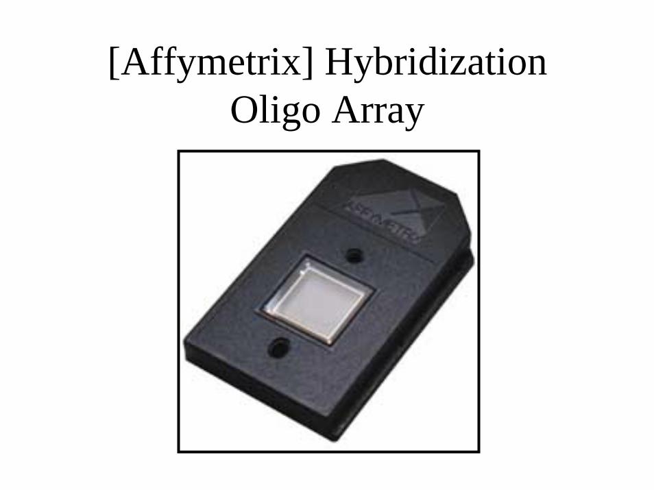
[Affymetrix] HybridizationOligo Array
Affymetrix GeneChips
• Contain multiple probes (spots) per gene• Probes corresponding to the same gene
must be processed to give a probe-set summary intensity for each gene
• Single label system– Higher reproducibility makes use of dual-labels
unnecessary

Affymetrix Arrays
• Single sample hybridized to each array• Each gene represented by a “probe set”
– One probe type per array “cell”– Typical probe is a 25-mer oligo– 11-16 PM:MM pairs per probe set
(PM = perfect match, MM = mismatch)

Source: Affymetrix website
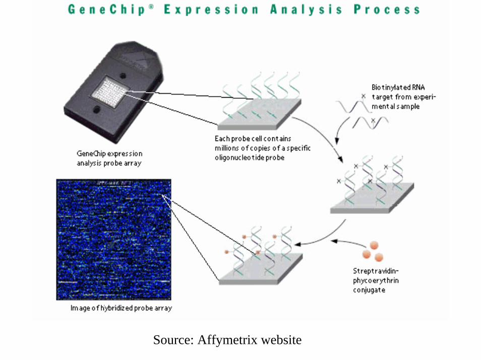
Source: Affymetrix website
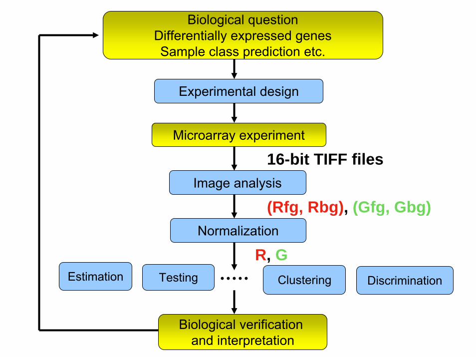
Biological questionDifferentially expressed genesSample class prediction etc.
Testing
Biological verification and interpretation
Microarray experiment
Estimation
Experimental design
Image analysis
Normalization
Clustering Discrimination
R, G
16-bit TIFF files
(Rfg, Rbg), (Gfg, Gbg)
Image Analysis
• Intensity is measured at fixed set of locations (pixels) arranged in rectangular patterns on the solid surface
• The distance between pixels is much less than the distance between probes
• The scanning microscope doesn’t know where the probes are; it just measures intensities at a fine grid of pixels
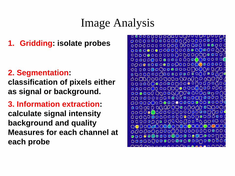
Image Analysis1. Gridding: isolate probes
2. Segmentation: classification of pixels either as signal or background. 3. Information extraction: calculate signal intensity background and quality Measures for each channel at each probe
Need for Normalization for Dual-Channel Array Data
• Unequal incorporation of labels – green better than red
• Unequal amounts of sample
• Unequal signal detection
• Dual-channel arrays are normalized separately to adjust for dye bias
• Affymetrix arrays are normalized relative to each other to equalize intensities

What Genes To Use For Normalization?
• Constantly expressed genes (house-keeping)• All genes on the array
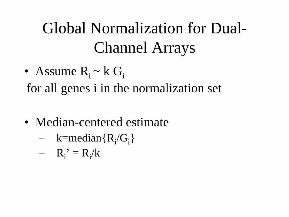
Global Normalization for Dual-Channel Arrays
• Assume Ri ~ k Gifor all genes i in the normalization set
• Median-centered estimate– k=median{Ri/Gi}– Ri’ = Ri/k
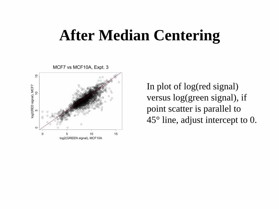
After Median Centering
MCF7 vs MCF10A, Expt. 3
log2(GREEN signal), MCF10A
log2
(RE
D s
igna
l), M
CF7
0 5 10 15
05
1015
In plot of log(red signal)versus log(green signal), if point scatter is parallel to 45° line, adjust intercept to 0.
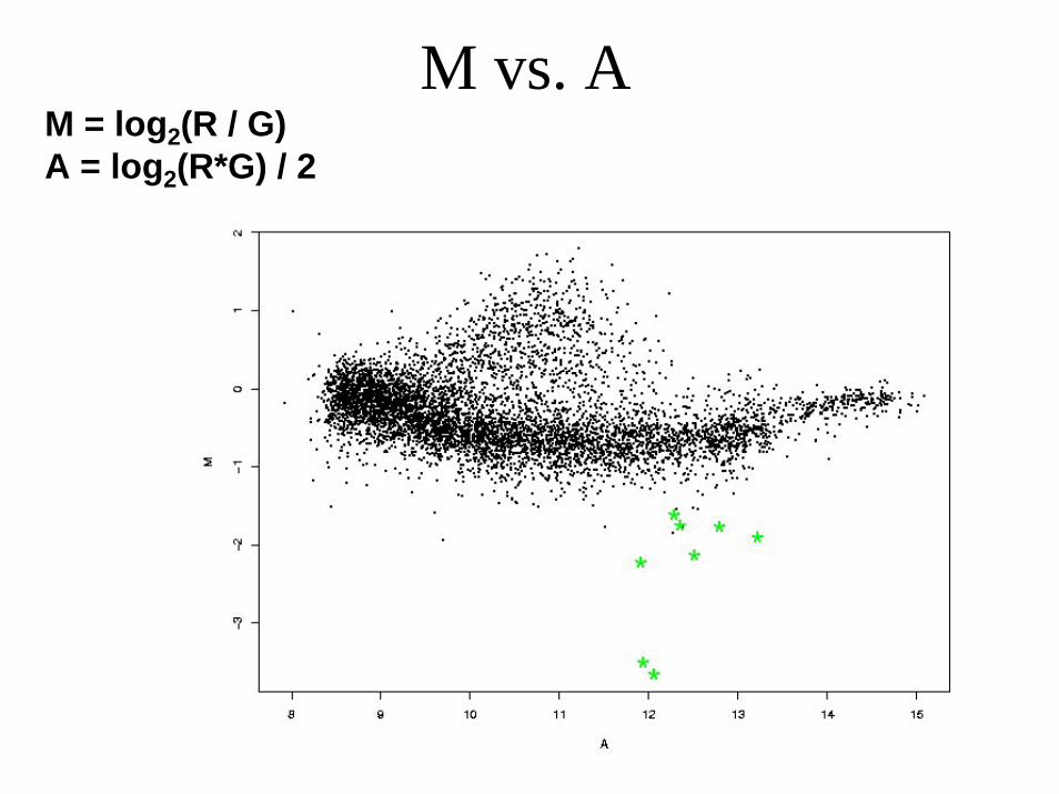
M vs. AM = log2(R / G)A = log2(R*G) / 2

Normalization - lowess• Global lowess

Normalisation - print-tip-group

M vs. A - after print-tip-group normalization
Normalization for Affymetrix Arrays
• Need– Variations in amount of sample or
environmental conditions– Variations in chip, hybridization, scanning
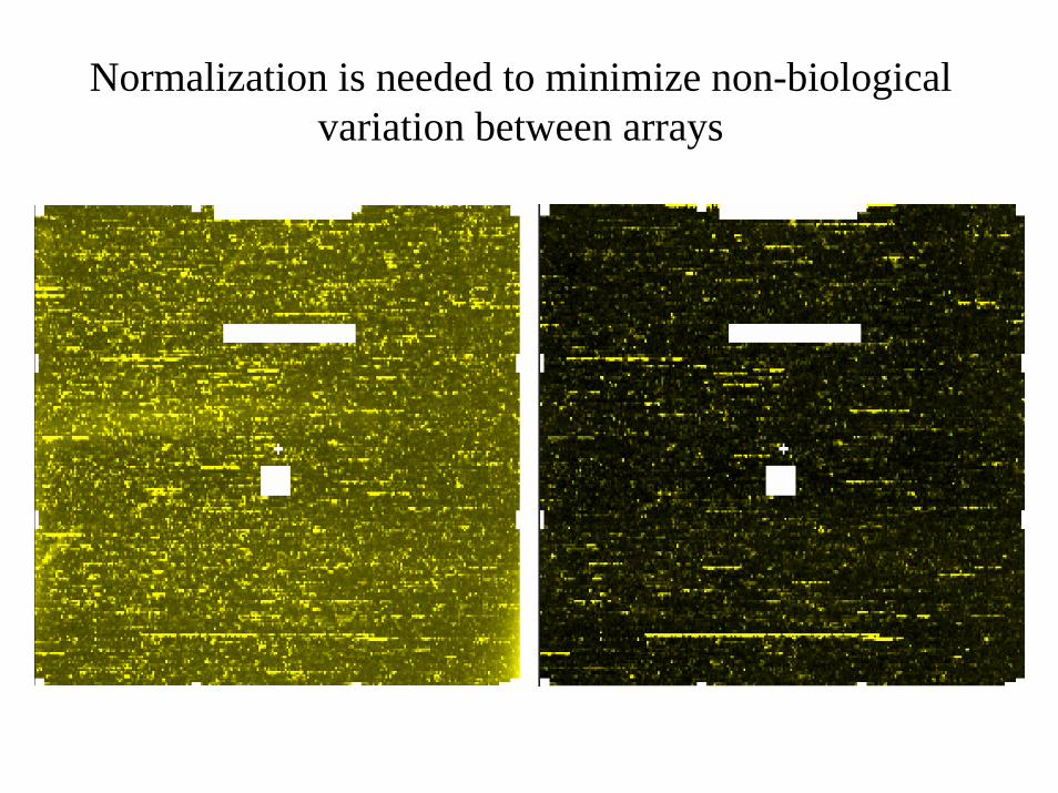
Normalization is needed to minimize non-biological variation between arrays

Normalization for Affymetrix Arrays
• Genes used– Affymetrix identifies housekeeping genes for some of
their new arrays• Methods
– Scale each array so that it’s median signal equals a target value
– Scale each array so that it’s median signal equals the median for a reference array
– Intensity dependent normalization using lowesssmoother based on ratios relative to a reference array
Spot Filtering Strategies
• Exclude if Signal < threshold in either channel
• Exclude if Signal < threshold in both channels
• If Min(R,G) < threshold – and Max(R,G) < threshold then exclude– Otherwise replace Min(R,G) by threshold
Gene Filtering Strategies• “Bad” values on too many arrays.
• Not differentially expressed across arrays.– Proportion of arrays < 1.5 fold different from median for
gene <20%

Affymetrix Arrays: Probe Set Summaries
MAS 4 Algorithm
• AvDiffi = Σj (PMij-MMij) / ni
for each probe set iSummation over ni =16-20 probes in probe set i
Excludes probe pairs that are more than 3 standard deviations from the average difference
Affymetrix Arrays: Probe Set (Gene) Summaries
MAS5 Algorithm
• Signal = Σwij (PMij-MMij)+
Uses Tukey biweights that continuously down-weights probe pairs whose difference is far from the average difference
Negative probe pair differences are modified to make them non-negative
(PMij-MMij)+ = max{ 0, PMij-MMij}
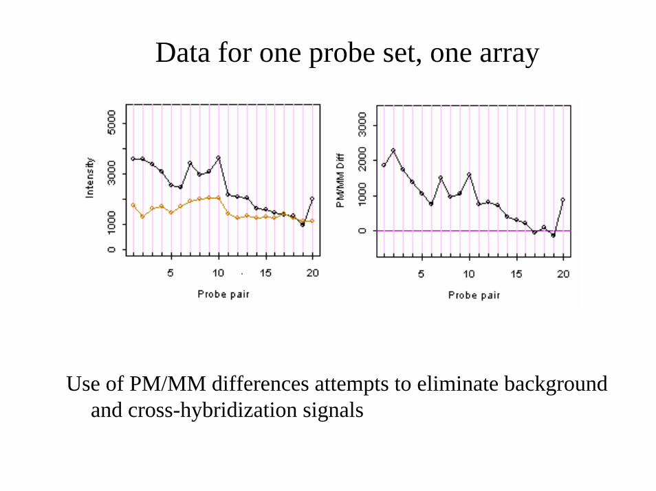
Data for one probe set, one array
Use of PM/MM differences attempts to eliminate background and cross-hybridization signals

Data for one gene in many arrays

Li-Wong Model
A multiplicative model for each gene:
: summary expression index for probe set on array k ,: probe sensitivity index for probe pair j
: random
jk jk k j jk
k
j
jk
PM MM θ φ ε
θφ
ε
− = +
( )k
normal errors
ˆ ˆ j jk jkj
PM MMθ φ= −∑
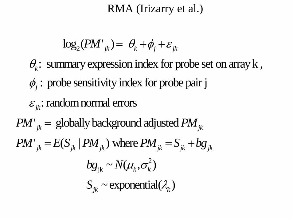
RMA (Irizarry et al.)
2 log ( ' )
: summary expression index for probe set on array k , : probe sensitivity index for probe pair j
: random normal errors
' globally back
jk k j jk
k
j
jk
jk
PM
PM
θ φ ε
θφ
ε
= + +
=
2jk
ground adjusted
' ( | ) where
~ ( , )
~exponential( )
jk
jk jk jk jk jk jk
k k
jk k
PM
PM E S PM PM S bg
bg N
S
µ σ
λ
= = +

RMA
• Estimate the background parameters globally for each array
• Estimate expression summaries θk for each probe set and each array k using Tukey’smedian polish algorithm

Affymetrix Present/Absent Calls
• Based on Mann-Whitney rank test of the hypothesis that the probe specific PM-MM differences are independent observations with median value zero

Design of Microarray Studies

Myth
• That microarray investigations should be unstructured data-mining adventures without clear objectives

Myth
• That the greatest challenge is managing the mass of microarray data
• Greater challenges are:– Effectively designing and properly analyzing
experiments that utilize microarray technology• Distinguishing hype and misinformation from sound
methodology• Avoiding software developed by individuals with no
qualifications for determining valid methodology
– Organizing and facilitating effective interdisciplinary collaboration with statisticians, clinicians & biologists
Myth
• That data mining is an appropriate paradigm for analysis of microarray data– find interesting patterns that give clear answers
to questions that were never asked
• That planning microarray investigations does not require “hypotheses” or clear objectives

• Good microarray studies have clear objectives, but not generally gene specific mechanistic hypotheses
• Design and analysis methods should be tailored to study objectives

Good Microarray Studies Have Clear Objectives
• Class Comparison– Find genes whose expression differs among
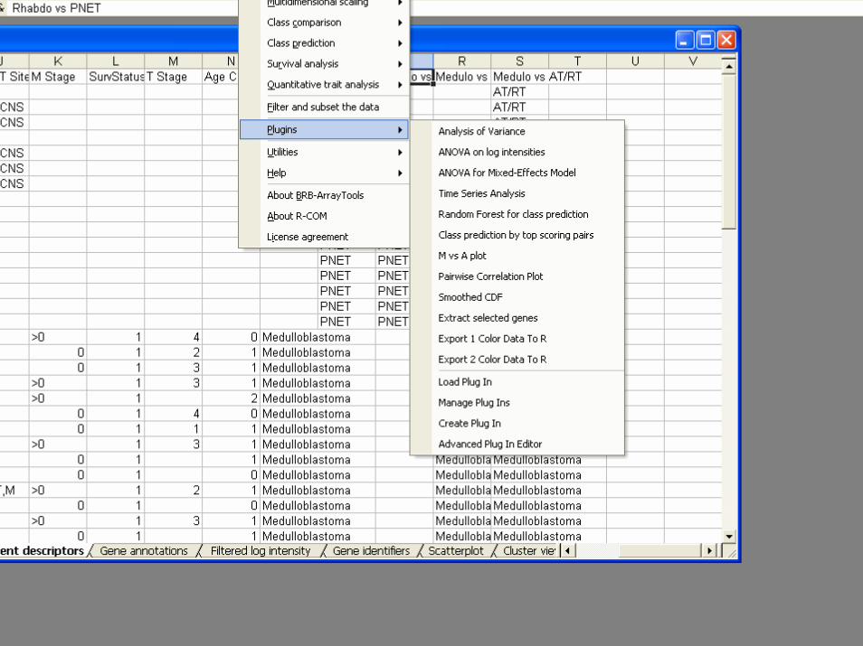
predetermined classes• Class Prediction
– Prediction of predetermined class (phenotype) using information from gene expression profile
• Class Discovery– Discover clusters of specimens having similar
expression profiles– Discover clusters of genes having similar expression
profiles
Class Comparison Examples
• Establish that expression profiles differ between two histologic types of cancer
• Identify genes whose expression level is altered by exposure of cells to an experimental drug
Class Prediction Examples
• Predict from expression profiles which patients are likely to experience severe toxicity from a new drug versus who will tolerate it well
• Predict which breast cancer patients will relapse within two years of diagnosis versus who will remain disease free
Class Discovery Examples
• Discover previously unrecognized subtypes of lymphoma
• Identify co-regulated genes
Design Considerations
• Sample and control selection • Levels of replication• Allocation of samples to (cDNA) array
experiments• Number of biological samples
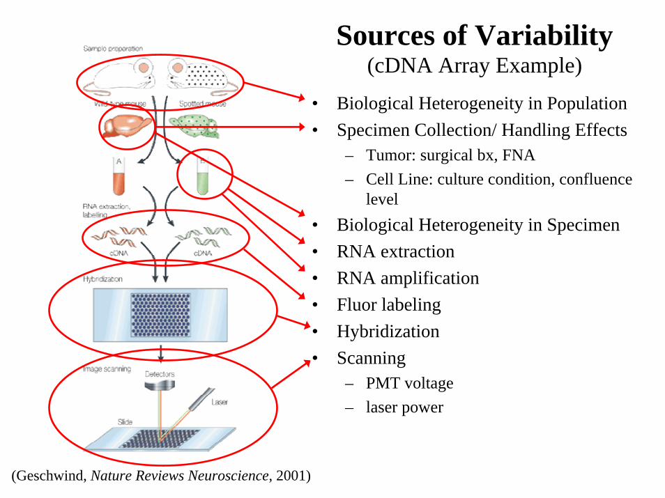
• Biological Heterogeneity in Population• Specimen Collection/ Handling Effects
– Tumor: surgical bx, FNA– Cell Line: culture condition, confluence
level• Biological Heterogeneity in Specimen• RNA extraction• RNA amplification• Fluor labeling• Hybridization• Scanning
– PMT voltage– laser power
Sources of Variability (cDNA Array Example)
(Geschwind, Nature Reviews Neuroscience, 2001)
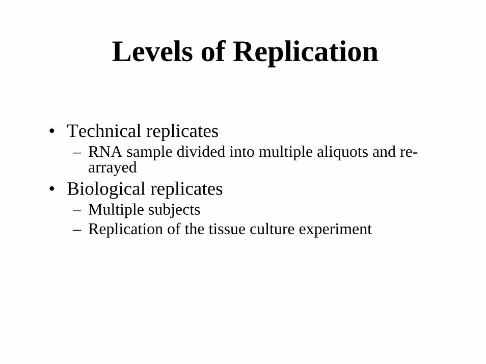
Levels of Replication
• Technical replicates– RNA sample divided into multiple aliquots and re-
arrayed• Biological replicates
– Multiple subjects – Re-growing the cells under the defined conditions

Technical Replicates of the Same RNA Sample
• Useful to establish that experimental technique and reagents are adequate– Not necessary for all samples
• Protection against bad hybridizations• Technical replicates improve precision for
comparing a given sample to another given sample. For comparing classes, however, it is more efficient to use a limited number of arrays for more independent biological samples than for technical replicates.

Levels of Replication
• For comparing classes, replication of samples should generally be at the “biological/subject” level because we want to make inference to the population of “cells/tissues/subjects”, not to the population of sub-samples of a single biological specimen.

Which Genes are Differentially Expressed In Two Conditions or Two
Tissues?• Not a clustering problem
– Global similarity measures generally used for clustering arrays may not distinguish classes
– Feature selection should be performed in a manner that controls the false discovery rate
• Supervised methods• Requires multiple biological samples from
each class
Myth
• That comparing tissues or experimental conditions is based on looking for red or green spots on a single array
• That comparing tissues or experimental conditions is based on using Affymetrix MAS software to compare two arrays– Many published statistical methods are limited
to comparing rna transcript profiles from two samples
Truth
• Comparing expression in two RNA samples tells you (at most) only about those two samples and may relate more to sample handling and assay artifacts than to biology. Robust knowledge requires multiple samples that reflect biological variability.
Class Comparison:Allocation of Specimens tocDNA Array Experiments
• Reference Design• Balanced Block Design
– Dobbin & Simon
• Loop Design – Kerr & Churchill
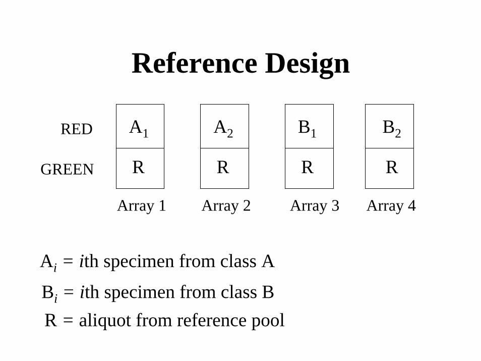
Reference Design
A1
R
A2 B1 B2
R
RED
R RGREEN
Array 1 Array 2 Array 3 Array 4
Ai = ith specimen from class A
Bi = ith specimen from class BR = aliquot from reference pool

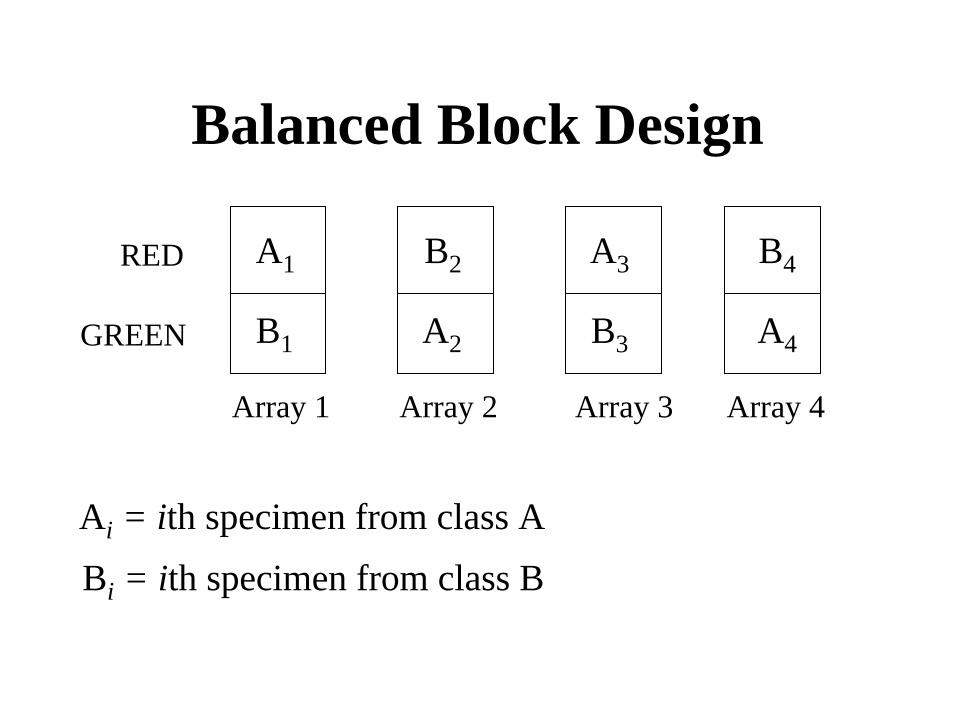
Balanced Block Design
A1
A2
B2 A3
B3
B4
A4
RED
B1GREEN
Array 1 Array 2 Array 3 Array 4
Ai = ith specimen from class A
Bi = ith specimen from class B
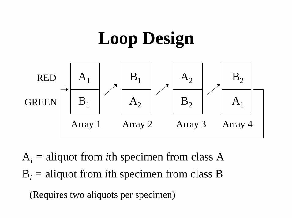
Loop Design
A1
A2
B1 A2
B2
B2
A1
RED
B1GREEN
Array 1 Array 2 Array 3 Array 4
Ai = aliquot from ith specimen from class ABi = aliquot from ith specimen from class B
(Requires two aliquots per specimen)

• Detailed comparisons of the effectiveness of designs: – Dobbin K, Simon R. Comparison of microarray designs
for class comparison and class discovery. Bioinformatics 18:1462-9, 2002
– Dobbin K, Shih J, Simon R. Statistical design of reverse dye microarrays. Bioinformatics 19:803-10, 2003
– Dobbin K, Simon R. Questions and answers on the design of dual-label microarrays for identifying differentially expressed genes, JNCI 95:1362-1369, 2003
Myth
• Common reference designs for two-color arrays are inferior to “loop” designs.
Truth• Common reference designs are effective for many
microarray studies. They are robust, permit comparisons among separate experiments, permit unplanned types of comparisons to be performed, permit cluster analysis and class prediction analysis.
• Loop designs are non-robust, are very inefficient for class discovery (clustering) analyses, are not applicable to class prediction analyses and do not easily permit inter-experiment comparisons.
• For simple two class comparison problems, balanced block designs are the most efficient and require many fewer arrays than reference designs. They are not appropriate for class discovery or class prediction and are more difficult to apply to more complicated class comparison problems.
Myth
• For two color microarrays, each sample of interest should be labeled once with Cy3 and once with Cy5 in dye-swap pairs of arrays.

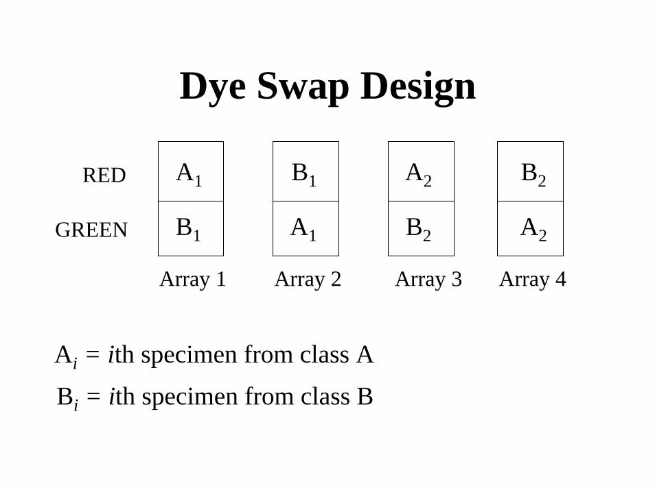
Dye Swap Design
A1
A1
B1 A2
B2
B2
A2
RED
B1GREEN
Array 1 Array 2 Array 3 Array 4
Ai = ith specimen from class A
Bi = ith specimen from class B

Dye Bias
• Average differences among dyes in label concentration, labeling efficiency, photon emission efficiency and photon detection are corrected by normalization procedures
• Gene specific dye bias may not be corrected by normalization
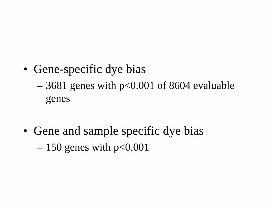
• Gene-specific dye bias– 3681 genes with p<0.001 of 8604 evaluable
genes
• Gene and sample specific dye bias– 150 genes with p<0.001
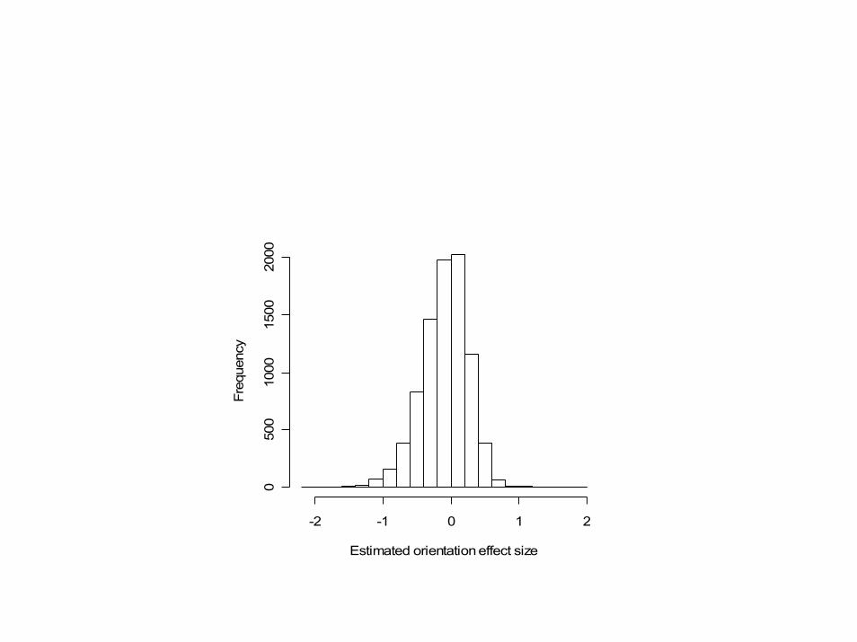
cDNA experiment estimated sizes of the gene-specific dye bias for each of the 8,604 genes. An effect of size 1 corresponds to a 2-fold change in
expression
Estimated orientation effect size
Freq
uenc
y
-2 -1 0 1 2
050
010
0015
0020
00
• Dye swap technical replicates of the same two rnasamples are rarely necessary.
• Using a common reference design, dye swap arrays are not necessary for valid comparisons of classes since specimens labeled with different dyes are never compared.
• For two-label direct comparison designs for comparing two classes, it is more efficient to balance the dye-class assignments for independent biological specimens than to do dye swap technical replicates
Balanced Block Design
A1
A2
B2 A3
B3
B4
A4
RED
B1GREEN
Array 1 Array 2 Array 3 Array 4
Ai = ith specimen from class A
Bi = ith specimen from class B
Dye Swap Design
A1
A1
B1 A2
B2
B2
A2
RED
B1GREEN
Array 1 Array 2 Array 3 Array 4
Ai = ith specimen from class A
Bi = ith specimen from class B
Balanced Block Designs for Two Classes
• Half the arrays have a sample from class 1 labeled with Cy5 and a sample from class 2 labeled with Cy3;
• The other half of the arrays have a sample from class 1 labeled with Cy3 and a sample from class 2 labeled with Cy5.
• Each sample appears on only one array. Dye swaps of the same rna samples are not necessary to remove dye bias and for a fixed number of arrays, dye swaps of the same rna samples are inefficient

Limitations of Balanced Block Designs
• One class comparison• Does not support cluster analysis• Requires ANOVA analysis of single
channel log intensities

cDNA Arrays: Reverse Fluor Experiments
Forward vs -Reverse logRatio MCF7 vs MCF10A
Avg. of 7 forward logRatios
-Avg
. of 3
reve
rse
logR
atio
s
-1 0 1
-10
1
PERSISTENT GREEN
PERSISTENT RED
Reverse Labeled Arrays
• Not necessary with reference design if you are not interested in direct comparison to internal reference– If reference rna is consistently labeled with the
same dye, dye bias effects all classes equally and does not bias comparison of classes.
– For clustering of specimens, the reference design should be used and no reverse labeled arrays are necessary.
Reverse Labeled Arrays
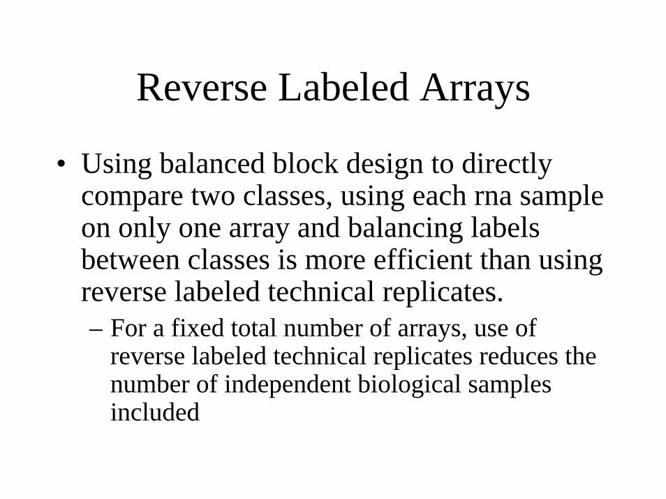
• Using balanced block design to directly compare two classes, using each rna sample on only one array and balancing labels between classes is more efficient than using reverse labeled technical replicates.– For a fixed total number of arrays, use of
reverse labeled technical replicates reduces the number of independent biological samples included

Reverse Labeled Arrays
• Necessary with reference design for some arrays if you are interested in direct comparison to internal reference– Gene specific dye bias not removed by
normalization
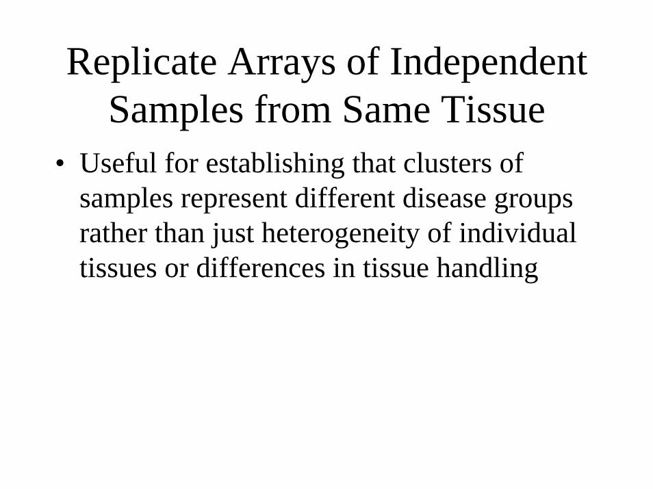
Replicate Arrays of Independent Samples from Same Tissue
• Useful for establishing that clusters of samples represent different disease groups rather than just heterogeneity of individual tissues or differences in tissue handling
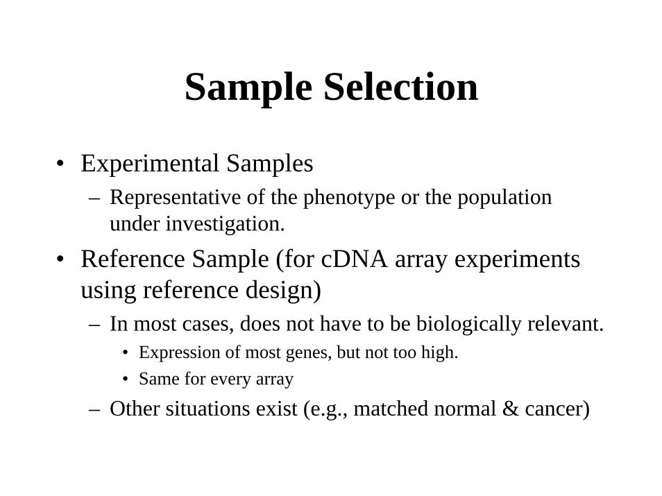
Sample Selection
• Experimental Samples– Representative of the phenotype or the population
under investigation.
• Reference Sample (for cDNA array experiments using reference design)– In most cases, does not have to be biologically relevant.
• Expression of most genes, but not too high.• Same for every array
– Other situations exist (e.g., matched normal & cancer)
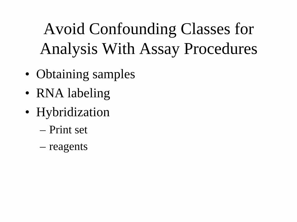
Avoid Confounding Classes for Analysis With Assay Procedures
• Obtaining samples• RNA labeling• Hybridization
– Print set– reagents

Experimental Design• Dobbin K, Simon R. Comparison of microarray designs for class
comparison and class discovery. Bioinformatics 18:1462-9, 2002• Dobbin K, Shih J, Simon R. Statistical design of reverse dye
microarrays. Bioinformatics 19:803-10, 2003• Dobbin K, Shih J, Simon R. Questions and answers on the design of
dual-label microarrays for identifying differentially expressed genes, JNCI 95:1362-69, 2003
• Simon R, Korn E, McShane L, Radmacher M, Wright G, Zhao Y. Design and analysis of DNA microarray investigations, Springer Verlag (2003)
• Simon R, Dobbin K. Experimental design of DNA microarray experiments. Biotechniques 34:1-5, 2002
• Simon R, Radmacher MD, Dobbin K. Design of studies with DNA microarrays. Genetic Epidemiology 23:21-36, 2002
• Dobbin K, Simon R. Sample size determination in microarray experiments for class comparison and prognostic classification. Biostatistics 6:27-38, 2005.

Good Microarray Studies Have Clear Objectives
• Class Comparison– Find genes whose expression differs among
predetermined classes• Class Prediction
– Prediction of predetermined class (phenotype) using information from gene expression profile
• Class Discovery– Discover clusters of specimens having similar
expression profiles– Discover clusters of genes having similar expression
profiles

Class Comparison and Class Prediction
• Not clustering problems– Global similarity measures generally used for
clustering arrays may not distinguish classes– Don’t control multiplicity or for distinguishing
data used for classifier development from data used for classifier evaluation
• Supervised methods• Requires multiple biological samples from
each class
Levels of Replication
• Technical replicates– RNA sample divided into multiple aliquots and re-
arrayed• Biological replicates
– Multiple subjects – Replication of the tissue culture experiment

• Biological conclusions generally require independent biological replicates. The power of statistical methods for microarray data depends on the number of biological replicates.
• Technical replicates are useful insurance to ensure that at least one good quality array of each specimen will be obtained.

Microarray Platforms for Class Comparison
• Single label arrays– Affymetrix GeneChips
• Dual label arrays– Common reference design– Other designs
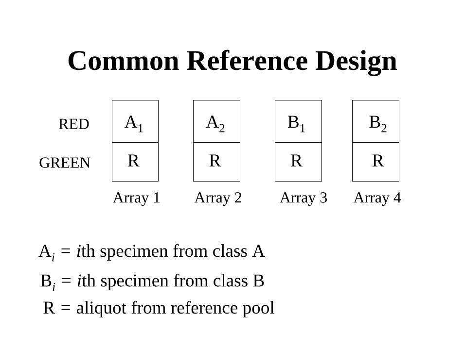
Common Reference Design
A1
R
A2 B1 B2
R
RED
R RGREEN
Array 1 Array 2 Array 3 Array 4
Ai = ith specimen from class A
Bi = ith specimen from class BR = aliquot from reference pool
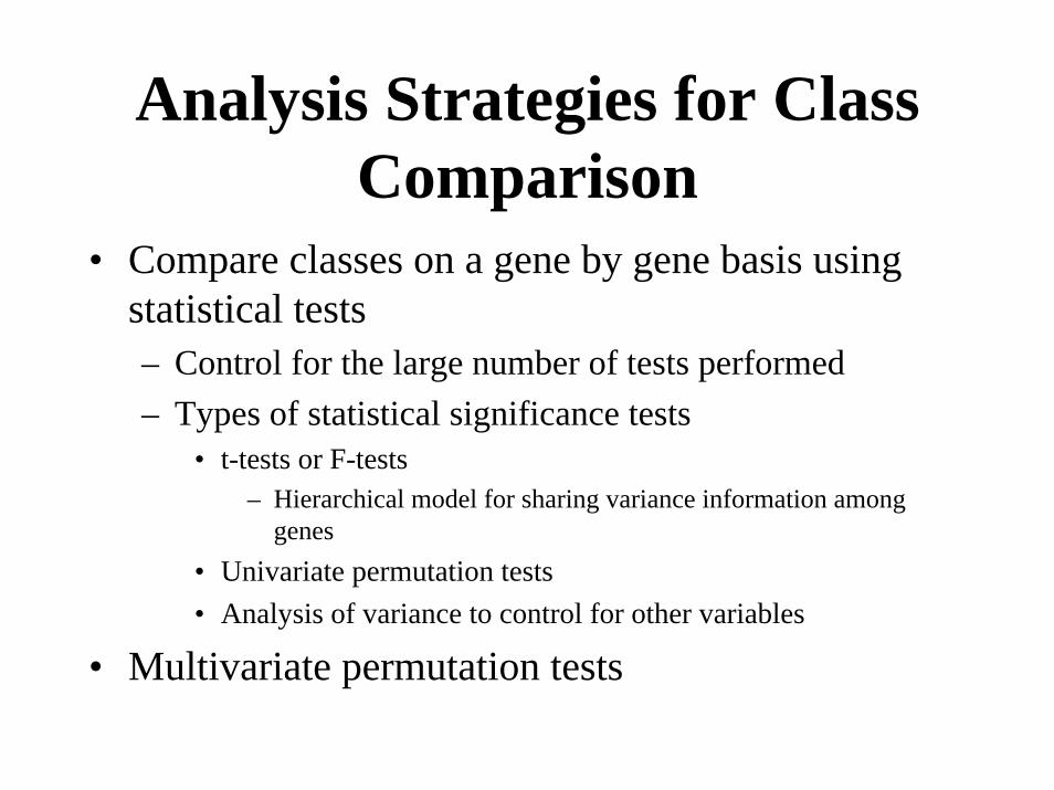
Analysis Strategies for Class Comparison
• Compare classes on a gene by gene basis using statistical tests– Control for the large number of tests performed– Types of statistical significance tests
• t-tests or F-tests– Hierarchical model for sharing variance information among
genes• Univariate permutation tests• Analysis of variance to control for other variables
• Multivariate permutation tests

Class Comparison Blocking
• Paired data– Pre-treatment and post-treatment samples of same
patient– Tumor and normal tissue from the same patient
• Blocking– Multiple animals in same litter– Any feature thought to influence gene expression
• Sex of patient• Batch of arrays
Technical Replicates
• Multiple arrays on alloquots of the same RNA sample
• Select the best quality technical replicate or• Average expression values
Controlling for Multiple Comparisons
• Bonferroni type procedures control the probability of making any false positive errors
• Overly conservative for the context of DNA microarray studies
Simple Control for Multiple Testing
• If each gene is tested for significance at level αand there are n genes, then the expected number of false discoveries is n α .– e.g. if n=1000 and α=0.001, then 1 false discovery– To control E(FD) ≤ u– Conduct each of k tests at level α = u/k
Simple Procedures
• Control E(FD) ≤ u– Conduct each of k tests at level u/k– e.g. To limit of 10 false discoveries in 10,000
comparisons, conduct each test at p<0.001 level• Control E(FDP) ≤ γ
– Benjamini-Hochberg procedure
False Discovery Rate (FDR)• FDR = Expected proportion of false
discoveries among the tests declared significant
• Studied by Benjamini and Hochberg (1995):
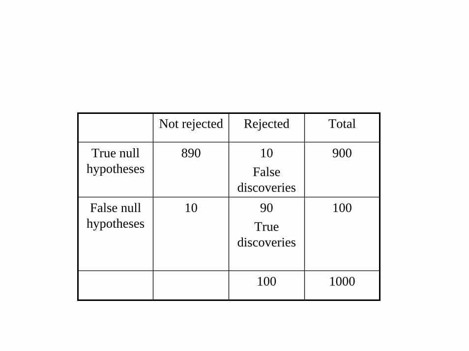
Not rejected Rejected Total
True null hypotheses
890 10 False
discoveries
900
False null hypotheses
10 90True
discoveries
100
100 1000
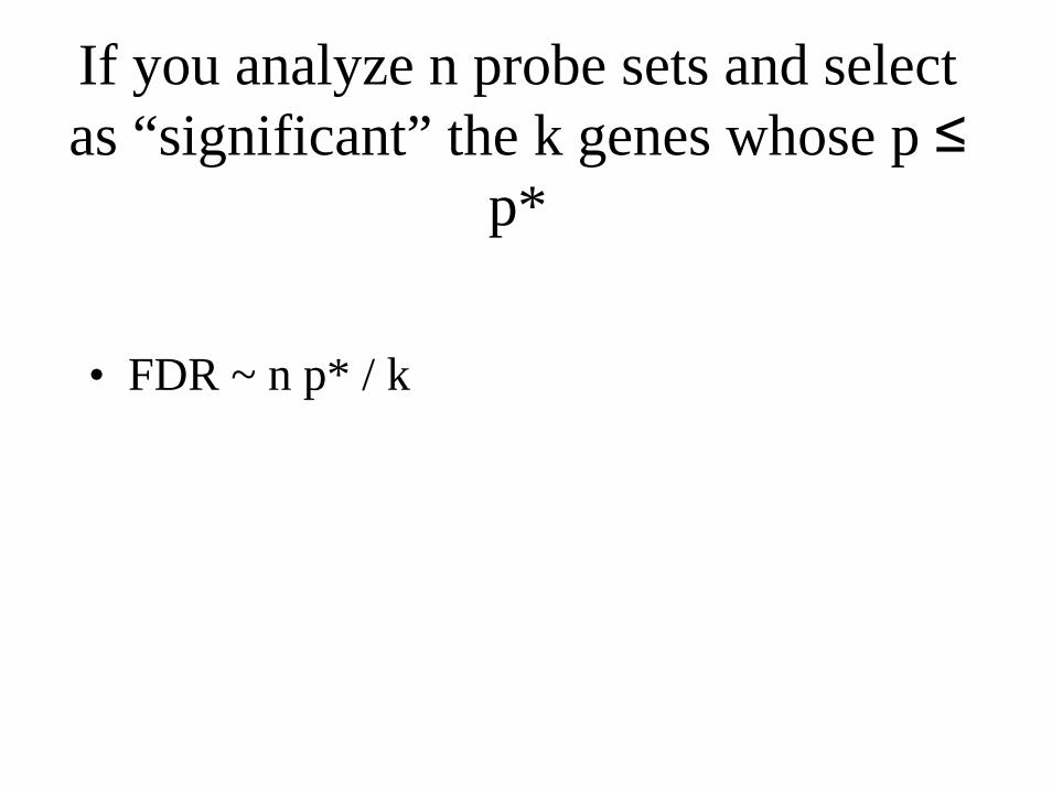
If you analyze n probe sets and select as “significant” the k genes whose p ≤
p*
• FDR ~ n p* / k
Limitations of Simple Procedures
• p values based on normal theory are not accurate in the extreme tails of the distribution
• Difficult to achieve extreme quantiles for permutation p values of individual genes
• Multiple comparisons controlled by adjustment of univariate (single gene) p values may not take advantage of correlation among genes

Gene-by-Gene Comparison of Classes
• t-test for comparing two classes– For dual-color arrays compare log-ratios, not ratios– For GeneChips compare log signals– tg=(meang1-meang2)/standard-errorg
– Standard-errorg= sg (1/n1 + 1/n2)1/2
– sg =within-class standard deviation– Computes statistical significance level as the probability of
obtaining a t value as large in absolute value as actually obtained if the two classes had the same true means and the sampling variation had a Gaussian distribution
– Gaussian distribution is symmetric “bell-shaped curve” which decreases at rate exp(-x2)
Limitations of Parametric t-test
• Expression values may not be approximately Gaussian
• t distribution approximation to the distribution of t under the null hypothesis is not accurate at the extreme tail of the distribution
• t distribution approximation is less accurate for small sample sizes
• Small sample size limits accuracy of estimation of sg– Few degrees of freedom for t limits statistic power for
detecting differences in mean expression levels

Gene-by-Gene Comparison of Classes
• Permutation t-test– Compute the t statistic comparing the two
classes for a gene but don’t use the Gaussian distribution assumption to translate the t value into a p value
– Consider all possible permutations of the labels of which arrays correspond to which class, holding fixed the number of total arrays in each class

Gene-by-Gene Comparison of Classes
• Permutation t-test (cont)– For each permutation of class labels re-compute
the t statistic comparing the classes with regard to a specific gene
– Determine the proportion of the permutations that gave a t value at least as large in absolute value as the one corresponding to the true data
– That proportion is the permutation p value
Limitation of Univariate Permutation Analysis
• Statistical significance level is limited by the number of possible permutations of the class labels. For small sample sizes, statistical significance at a stringent significance level (e.g. p<0.001) either cannot be achieved or is achieved with limited statistical power
Gene-by-Gene Comparison of Classes
• All of these tests assume that the different arrays are independent. Hence replicate arrays must be either averaged, or the best quality one selected for inclusion in the analysis, or a more complex ANOVA model be used for analysis
Gene-by-Gene Comparison of Classes
• F-test– The generalization of the t-test when there are more
than 2 classes to compare.• Significance indicates that the class means are more different
than one expects by chance but it does not indicate which classes are different from which other classes.
• The statistically significant genes may differ with regard to the patterns of differences among classes that they show. Clustering the set of significant genes is useful to sort the genes into sets with uniform patterns.
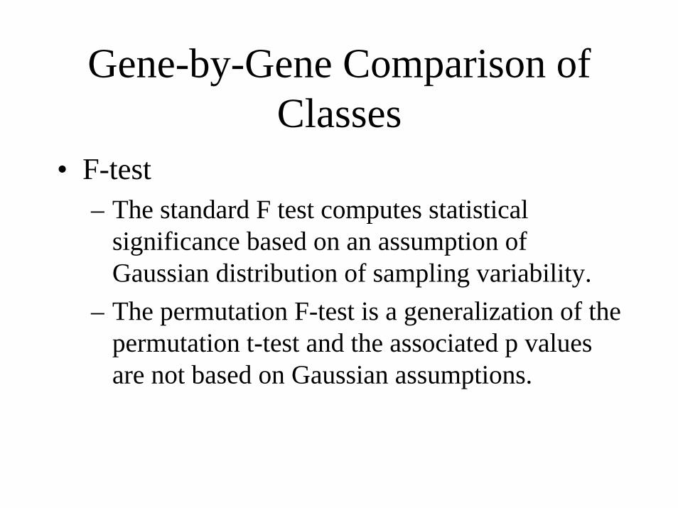
Gene-by-Gene Comparison of Classes
• F-test– The standard F test computes statistical
significance based on an assumption of Gaussian distribution of sampling variability.
– The permutation F-test is a generalization of the permutation t-test and the associated p values are not based on Gaussian assumptions.
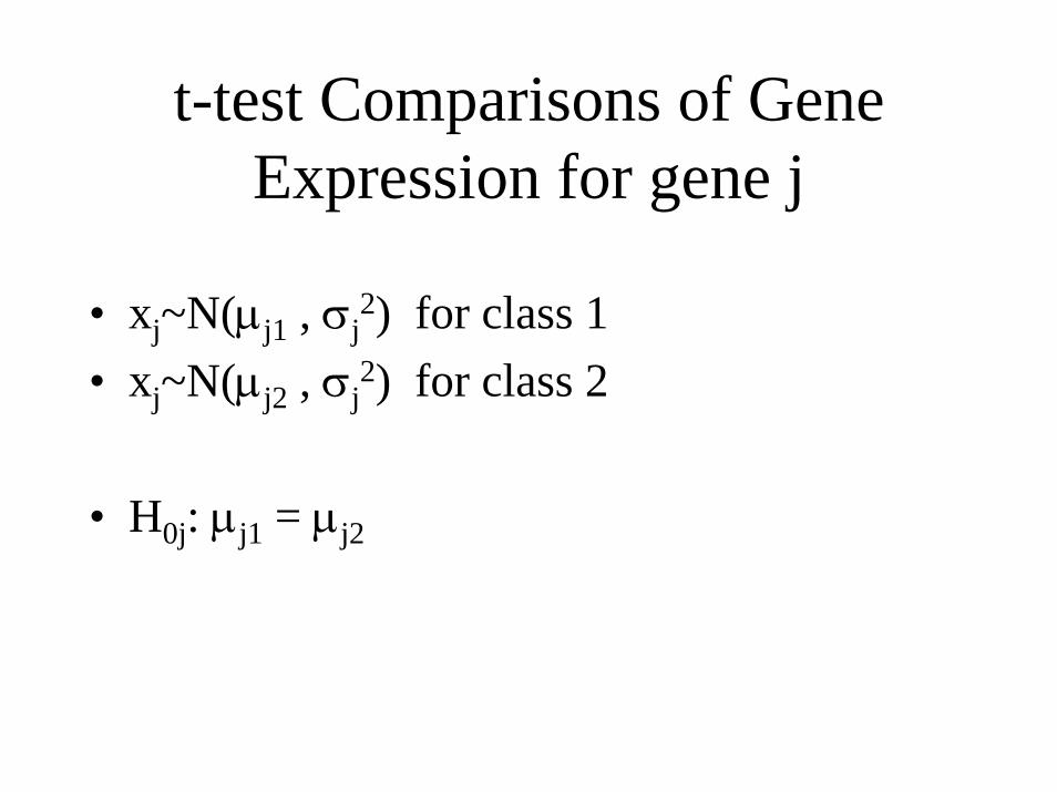
t-test Comparisons of Gene Expression for gene j
• xj~N(µj1 , σj2) for class 1
• xj~N(µj2 , σj2) for class 2
• H0j: µj1 = µj2
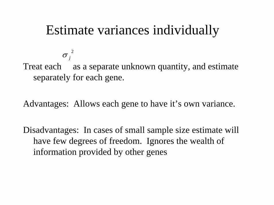
Estimate variances individually
Treat each as a separate unknown quantity, and estimate separately for each gene.
Advantages: Allows each gene to have it’s own variance.
Disadvantages: In cases of small sample size estimate will have few degrees of freedom. Ignores the wealth of information provided by other genes
2jσ
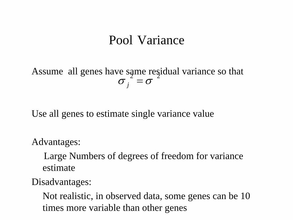
Pool Variance
Assume all genes have same residual variance so that
Use all genes to estimate single variance value
Advantages:Large Numbers of degrees of freedom for variance estimate
Disadvantages:Not realistic, in observed data, some genes can be 10 times more variable than other genes
22 σσ =j
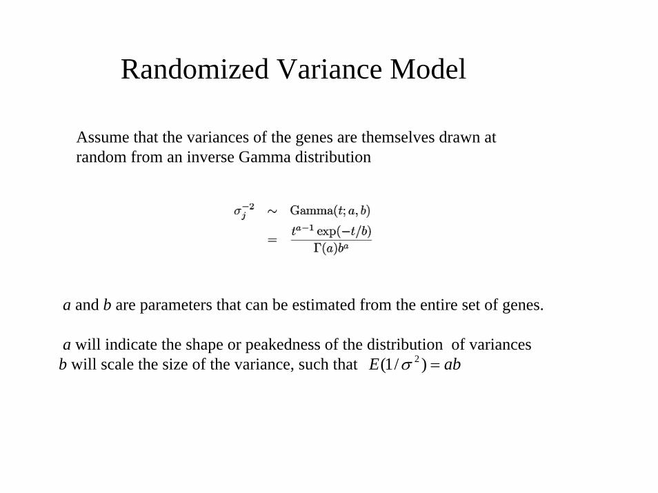
Randomized Variance Model
Assume that the variances of the genes are themselves drawn at random from an inverse Gamma distribution
a and b are parameters that can be estimated from the entire set of genes.
a will indicate the shape or peakedness of the distribution of variancesb will scale the size of the variance, such that abE =)/1( 2σ

Randomized Variance Model
Advantages:• Allows for the variance to realistically vary between genes
• Uses information from all genes to contribute to variance estimates increasing reliability of estimate.
Disadvantages:• Requires additional assumptions about the distribution of the
variances
• Estimates of variance may still be noisy
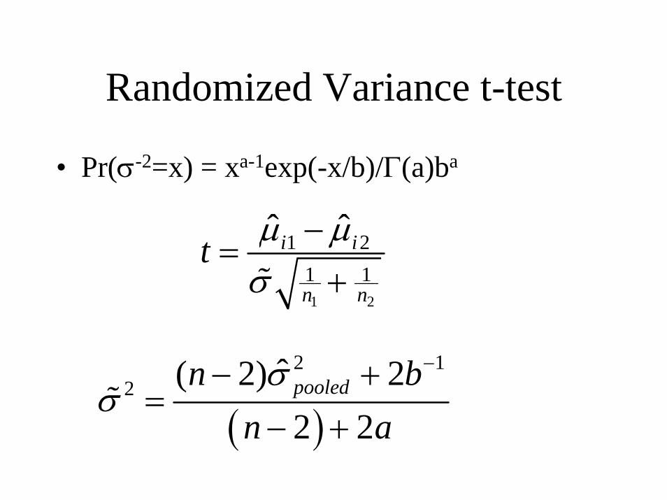
Randomized Variance t-test
• Pr(σ-2=x) = xa-1exp(-x/b)/Γ(a)ba
1 2
1 21 1
ˆ ˆi i
n n
t µ µσ
−=
+
( )
2 12 ˆ( 2) 2
2 2pooledn b
n aσ
σ−− +
=− +
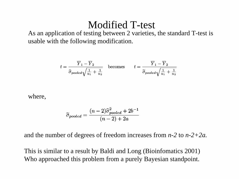
Modified T-testAs an application of testing between 2 varieties, the standard T-test is usable with the following modification.
where,
and the number of degrees of freedom increases from n-2 to n-2+2a.
This is similar to a result by Baldi and Long (Bioinfomatics 2001)Who approached this problem from a purely Bayesian standpoint.
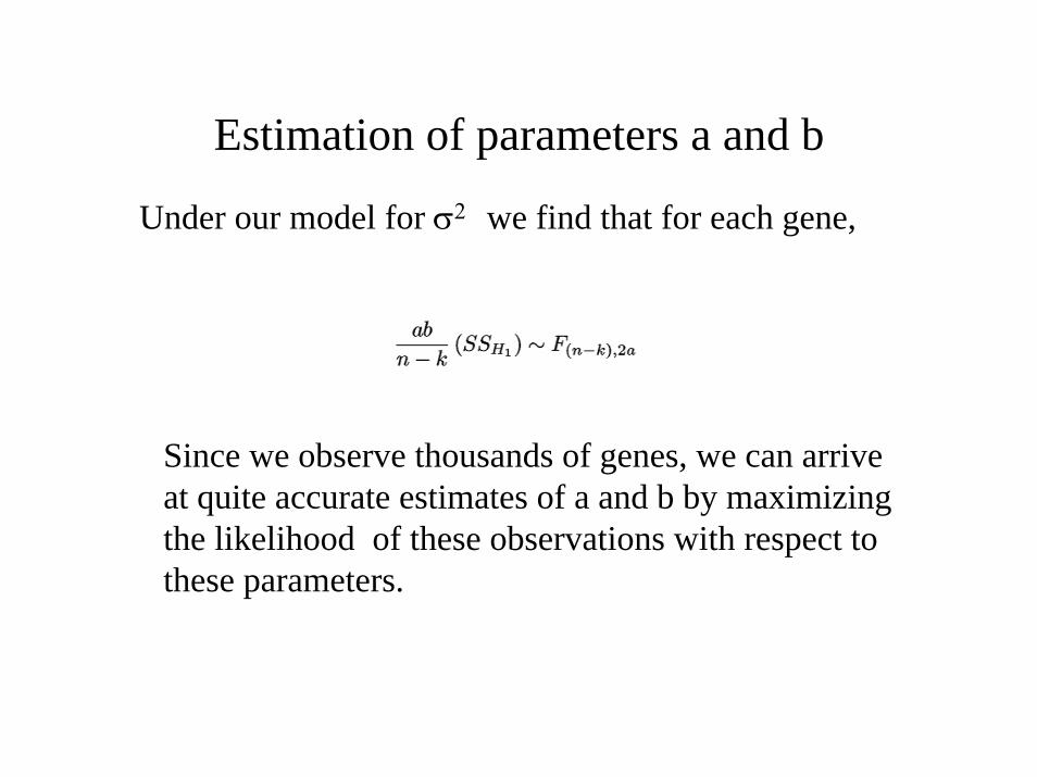
Estimation of parameters a and b
Under our model for σ2 we find that for each gene,
Since we observe thousands of genes, we can arrive at quite accurate estimates of a and b by maximizing the likelihood of these observations with respect to these parameters.
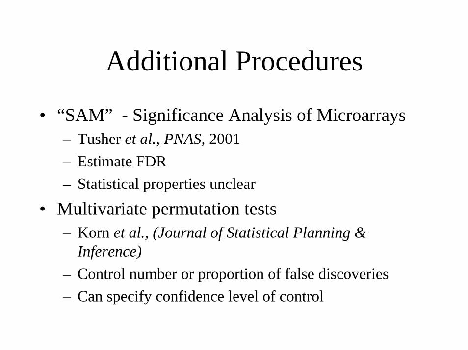
Additional Procedures
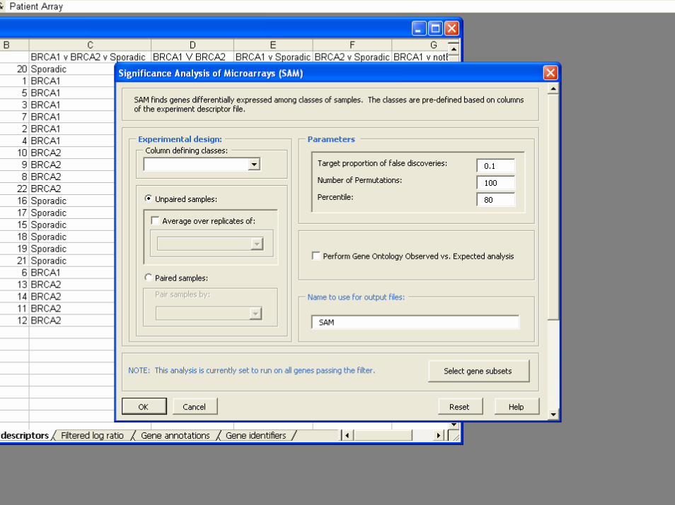
• “SAM” - Significance Analysis of Microarrays– Tusher et al., PNAS, 2001– Estimate FDR– Statistical properties unclear
• Multivariate permutation tests– Korn et al., (Journal of Statistical Planning &
Inference)– Control number or proportion of false discoveries– Can specify confidence level of control
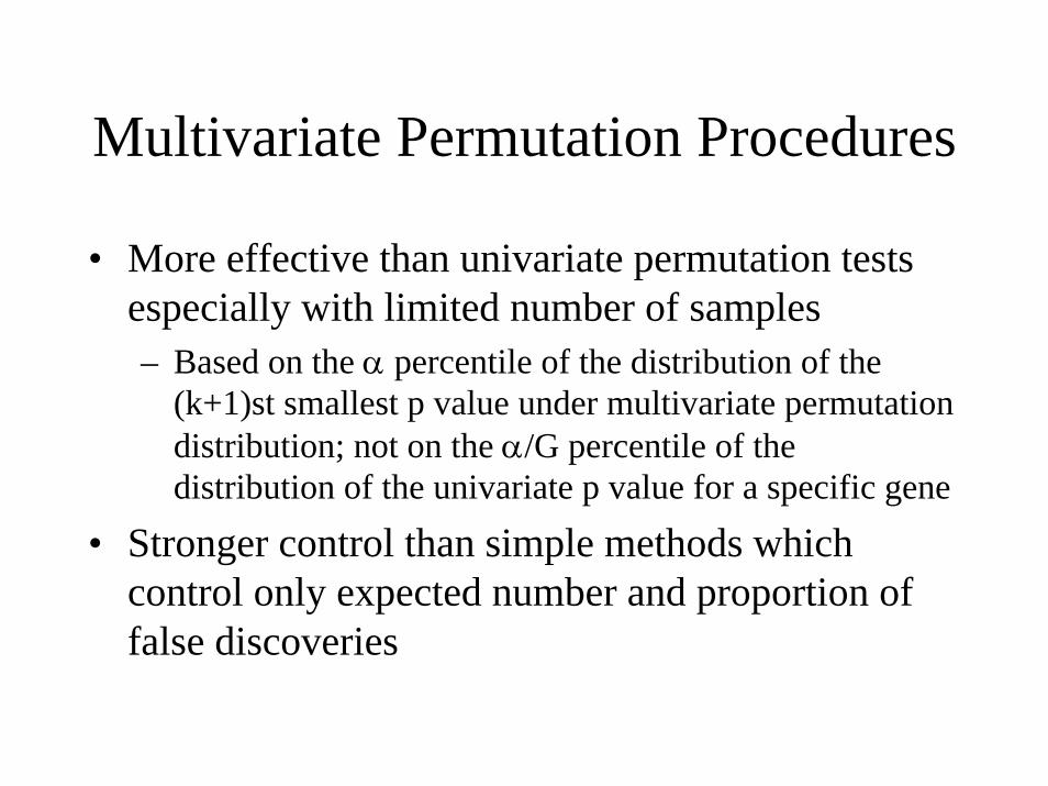
Multivariate Permutation Procedures
• More effective than univariate permutation tests especially with limited number of samples– Based on the α percentile of the distribution of the
(k+1)st smallest p value under multivariate permutation distribution; not on the α/G percentile of the distribution of the univariate p value for a specific gene
• Stronger control than simple methods which control only expected number and proportion of false discoveries
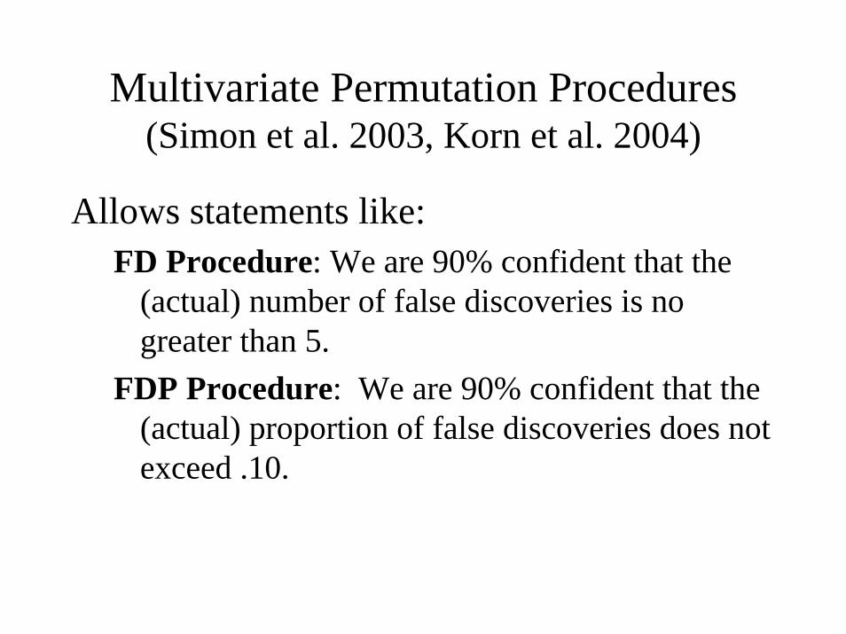
Multivariate Permutation Procedures(Simon et al. 2003, Korn et al. 2004)
Allows statements like:FD Procedure: We are 90% confident that the
(actual) number of false discoveries is no greater than 5.
FDP Procedure: We are 90% confident that the (actual) proportion of false discoveries does not exceed .10.
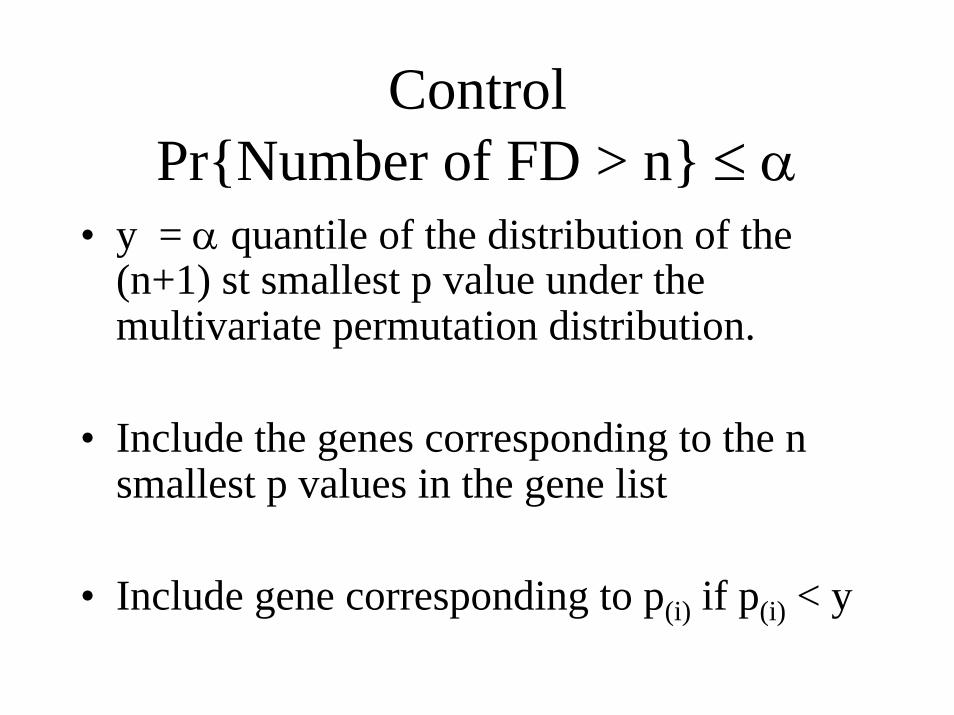
Control Pr{Number of FD > n} ≤ α
• y = α quantile of the distribution of the (n+1) st smallest p value under the multivariate permutation distribution.
• Include the genes corresponding to the n smallest p values in the gene list
• Include gene corresponding to p(i) if p(i) < y
Multivariate Permutation Tests
• Distribution-free – even if they use t statistics
• Preserve/exploit correlation among tests by permuting each profile as a unit
• More effective than univariate permutation tests especially with limited number of samples

Control Pr{FDP > γ} ≤ α
• Determine y(u) = α quantile of the distribution of the (u+1)st smallest p value under the multivariate permutation distribution.– For u = 1,2,3, …
• Include in the list of differentially expressed genes the gene corresponding to the i’th smallest p value as long as p(i) < y(⎣γ i⎦)– Sequentially for i = 1,2, …– ⎣γ i⎦ = largest integer less than or equal to γ i
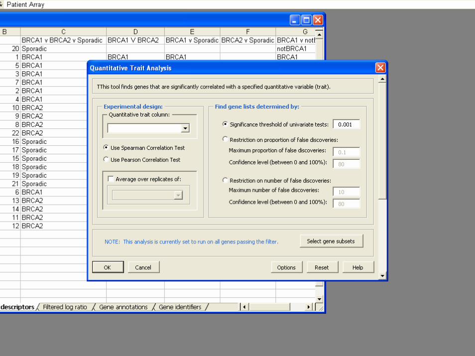
Quantitative trait tool• Selects genes which are univariately correlated
with a quantitative trait such as age.• Controls number and proportion of false
discoveries in entire list: uses a multivariate permutation test which takes advantage of the correlation among genes.
• Produces a gene list which can be used for further analysis.
Survival analysis tools• Find Genes Correlated with Survival tool, selects
genes which are univariately correlated with survival
• Controls number and proportion of false discoveries in entire list: uses a multivariate permutation test which takes advantage of the correlation among genes
• Produces a gene list which can be used for further analysis
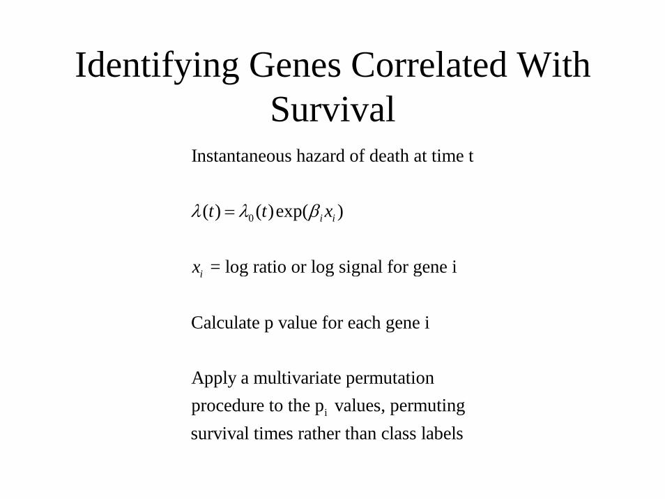
Identifying Genes Correlated With Survival
0
i
Instantaneous hazard of death at time t
( ) ( )exp( )
= log ratio or log signal for gene i
Calculate p value for each gene i
Apply a multivariate permutation procedure to the p values, permuting
i i
i
t t x
x
λ λ β=
survival times rather than class labels

Gene Set Expression Comparison
• Compute p value of differential expression for each gene in a gene set (k=number of genes)
• Compute a summary (S) of these p values• Determine whether the value of the summary test statistic
S is more extreme than would be expected from a random sample of k genes (probe-sets) on that platform
• Two types of summaries provided– Average of log p values– Kolmogorov-Smirnov statistic; largest distance between the
cumulative distribution of the p values and the uniform distribution expected if none of the genes were differentially expressed
Gene Set Expression Comparison
• p value for significance of summary statistic need not be as extreme as .001 usually, because the number of gene sets analyzed is usually much less than the number of individual genes analyzed
• Conclusions of significance are for gene sets in this tool, not for individual genes

Comparison of Gene Set Expression Comparison to O/E Analysis in Class
Comparison
• Gene set expression tool is based on all genes in a set, not just on those significant at some threshold value
• O/E analysis does not provide statistical significance for gene sets

Fallacy of Clustering Classes Based on Selected Genes
• Even for arrays randomly distributed between classes, genes will be found that are “significantly” differentially expressed
• With 8000 genes measured, 400 false positives will be differentially expressed with p < 0.05
• Arrays in the two classes will necessarily cluster separately when using a distance measure based on genes selected to distinguish the classes
Class Prediction
• Predict membership of a specimen into pre-defined classes– Disease vs normal– Poor vs good response to treatment– Long vs short survival
Traditional Approach for Marker Development
• Focus on candidate protein involved in disease pathogenesis
• Develop assay• Conduct retrospective study of whether
marker is prognostic using available specimens
• Marker dies because– Therapeutic relevance not established– Inter-laboratory reproducibility not established
Genomic Approach to Diagnostic/Prognostic Marker Development
• Select therapeutically relevant population– Node negative well staged breast cancer patients who
have not received chemotherapy and have long follow-up
– Early stage ovarian cancer patients and normal controls• Perform genome wide expression profiling• Develop multi-gene/protein predictor of outcome• Obtain unbiased estimate of prediction accuracy• Independently confirm results
Limitations of Genomic Approach
• Difficulty relating differentially expressed genes to cause of disease– or to real therapeutic targets
• Availibility of tissue and clinical follow-up for therapeutically relevant questions– Many studies address overly simple problems or
heterogeneous non-therapeutically relevant populations– Inclusion of advance disease patients– Comparing completely different types of cancer
Limitations of Genomic Approach
• Difficulty in performing adequate validation studies
• Lack of inter-laboratory reproducibility evaluations
Class Prediction Model• Given a sample with an expression profile vector x of log-
ratios or log signals and unknown class. • Predict which class the sample belongs to• The class prediction model is a function f which maps from
the set of vectors x to the set of class labels {1,2} (if there are two classes).
• f generally utilizes only some of the components of x (i.e. only some of the genes)
• Specifying the model f involves specifying some parameters (e.g. regression coefficients) by fitting the model to the data (learning the data).

Components of Class Prediction
• Feature (gene) selection– Which genes will be included in the model
• Select model type – E.g. DLDA, Nearest-Neighbor, …
• Fitting parameters (regression coefficients) for model
Class Prediction Paradigm
• Select features (F) to be included in predictive model using training data in which class membership of the samples is known
• Fit predictive model containing features F using training data– Diagonal linear discriminant analysis– Neural network
• Evaluate predictive accuracy of model on completely independent data not used in any way for development of the model

Feature Selection• Key component of supervised analysis• Genes that are differentially expressed among the classes
at a significance level α (e.g. 0.01) – The α level is selected to control the number of genes in the
model, not to control the false discovery rate• Methods for class prediction are different than those for class
comparison– The accuracy of the significance test used for feature selection is
not of major importance as identifying differentially expressed genes is not the ultimate objective
– For survival prediction, the genes with significant univariate Cox PH regression coefficients
Feature Selection
• Small subset of genes which together give most accurate predictions – Step-up regression– Combinatorial optimization algorithms
• Genetic algorithms
• Principal components of genes• Gene cluster averages
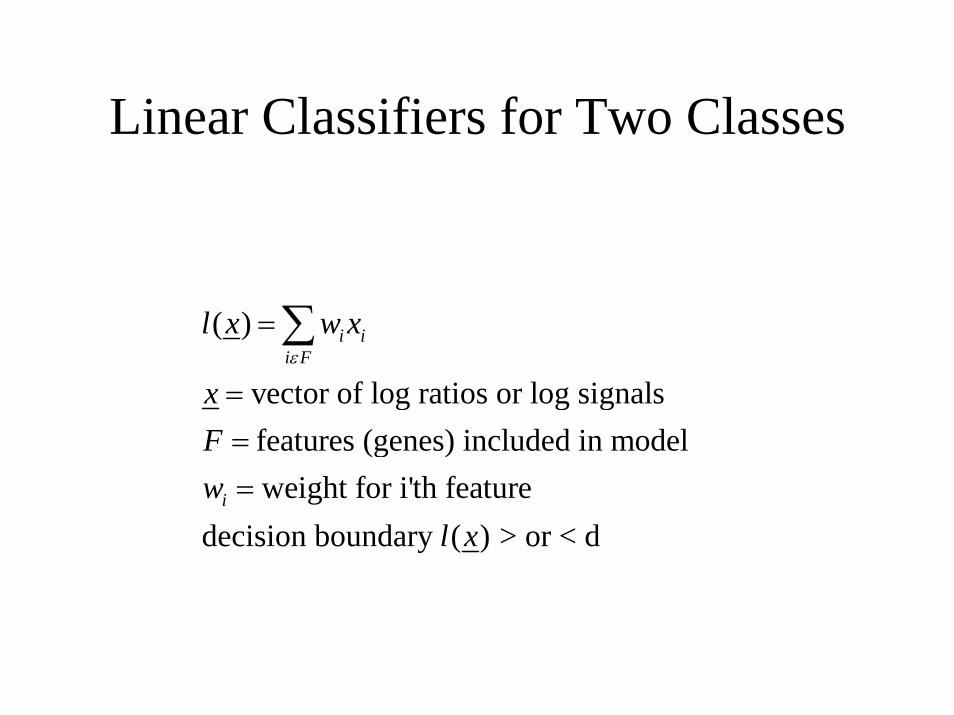
Linear Classifiers for Two Classes
( )
vector of log ratios or log signalsfeatures (genes) included in modelweight for i'th feature
decision boundary ( ) > or < d
i ii F
i
l x w x
xFw
l x
ε
=
===
∑

Linear Classifiers for Two Classes
• Compound covariate predictor
Instead of for DLDA
(1) (2)
ˆi i
ii
x xwσ−
∝
(1) (2)
2ˆi i
ii
x xwσ−
∝

Linear Classifiers for Two Classes
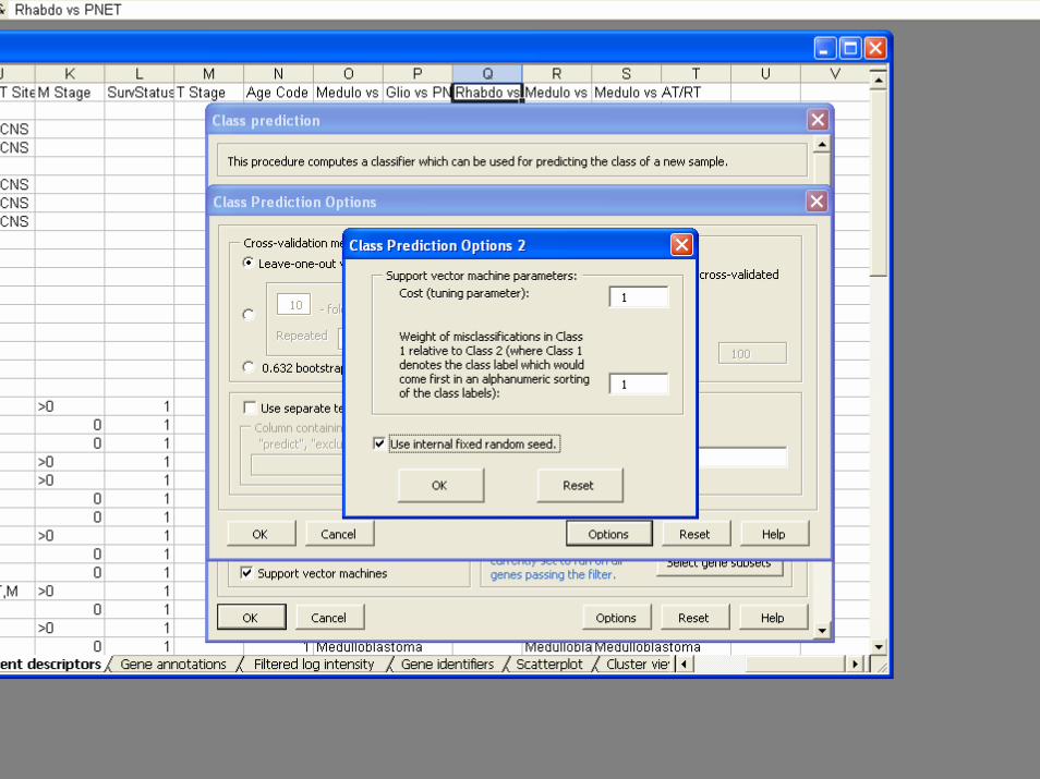
• Support vector machines with inner product kernel are linear classifiers with weights determined to minimize errors
• Perceptrons with principal components as input are linear classifiers with no well defined criterion for defining weights

Advantages of Simple Linear Classifiers
• Do not over-fit data– Incorporate influence of multiple variables
without attempting to select the best small subset of variables
– Do not attempt to model the multivariate interactions among the predictors and outcome

Evaluating a Classifier
• “Prediction is difficult, especially the future.”– Neils Bohr
• Fit of a model to the same data used to develop it is no evidence of prediction accuracy for independent data.

Split-Sample Evaluation
• Training-set– Used to select features, select model type, determine
parameters and cut-off thresholds
• Test-set– Withheld until a single model is fully specified using
the training-set.– Fully specified model is applied to the expression
profiles in the test-set to predict class labels. – Number of errors is counted

Split-Sample Evaluation
• Used for Rosenwald et al. study of prognosis in DLBL lymphoma.– 200 cases training-set– 100 cases test-set
Leave-one-out Cross Validation
• Leave-one-out cross-validation simulates the process of separately developing a model on one set of data and predicting for a test set of data not used in developing the model
spec
imen
s
log-expression ratios
full data set
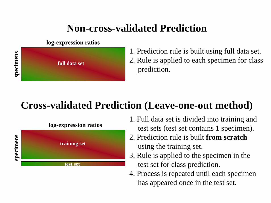
Non-cross-validated Prediction
1. Prediction rule is built using full data set.2. Rule is applied to each specimen for class
prediction.
training set
test set
spec
imen
s
log-expression ratios
Cross-validated Prediction (Leave-one-out method)1. Full data set is divided into training and
test sets (test set contains 1 specimen).2. Prediction rule is built from scratch
using the training set.3. Rule is applied to the specimen in the
test set for class prediction. 4. Process is repeated until each specimen
has appeared once in the test set.

Cross-validated Misclassification Rate of Any Multivariable Classifier
• Omit sample 1– Develop multivariate classifier from scratch on
training set with sample 1 omitted– Predict class for sample 1 and record whether
prediction is correct
Cross-validated Misclassification Rate of Any Multivariate Classifier
• Repeat analysis for training sets with each single sample omitted one at a time
• e = number of misclassifications determined by cross-validation
• Cross validation is only valid if the training set is not used in any way in the development of the model. Using the complete set of samples to select genes violates this assumption and invalidates cross-validation.
• With proper cross-validation, the model must be developed from scratch for each leave-one-out training set. This means that gene selection must be repeated for each leave-one-out training set.
• The cross-validated estimate of misclassification error applies to the model building process, not to the particular model or the particular set of genes used in the model.
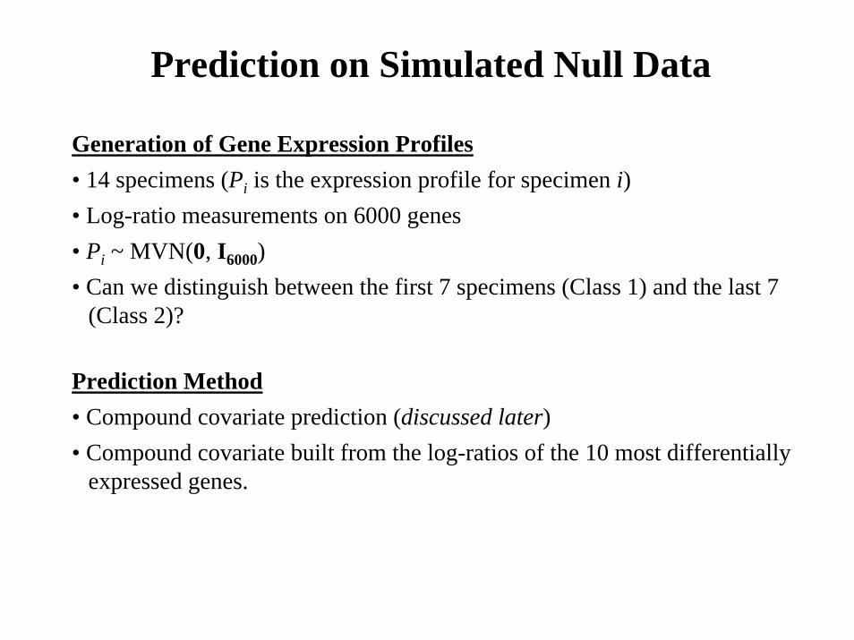
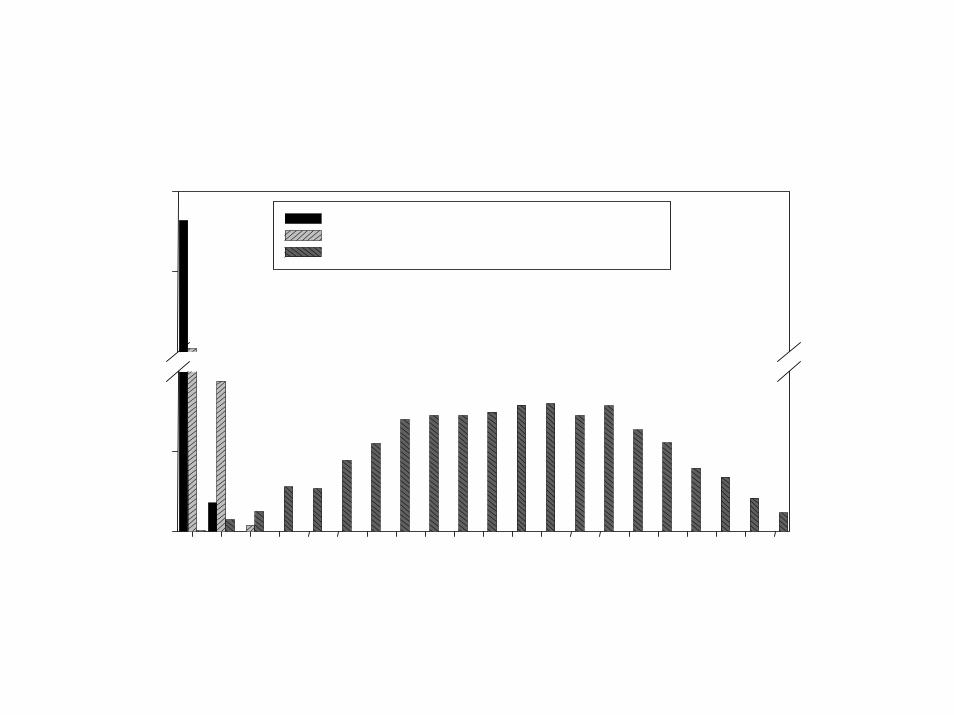
Prediction on Simulated Null Data
Generation of Gene Expression Profiles• 14 specimens (Pi is the expression profile for specimen i)• Log-ratio measurements on 6000 genes• Pi ~ MVN(0, I6000)• Can we distinguish between the first 7 specimens (Class 1) and the last 7
(Class 2)?
Prediction Method• Compound covariate prediction (discussed later)• Compound covariate built from the log-ratios of the 10 most differentially
expressed genes.
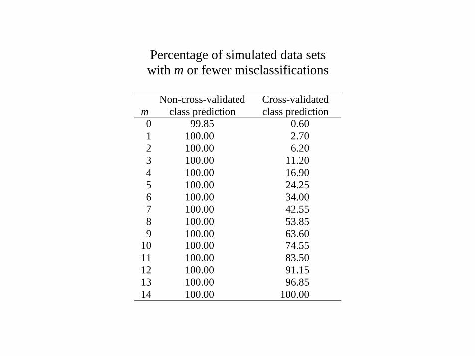
Percentage of simulated data setswith m or fewer misclassifications
mNon-cross-validated
class predictionCross-validatedclass prediction
0 99.85 0.601 100.00 2.702 100.00 6.203 100.00 11.204 100.00 16.905 100.00 24.256 100.00 34.007 100.00 42.558 100.00 53.859 100.00 63.60
10 100.00 74.5511 100.00 83.5012 100.00 91.1513 100.00 96.8514 100.00 100.00
Incomplete (incorrect) Cross-Validation
• Biologists and computer scientists are using all the data to select genes and then cross-validating only the parameter estimation (learning) component of model development– Highly biased– Many published complex methods which make strong
claims based on incorrect cross-validation. • Frequently seen in complex feature set selection algorithms• Also seen in proposals for decision tree classifiers and neural
networks
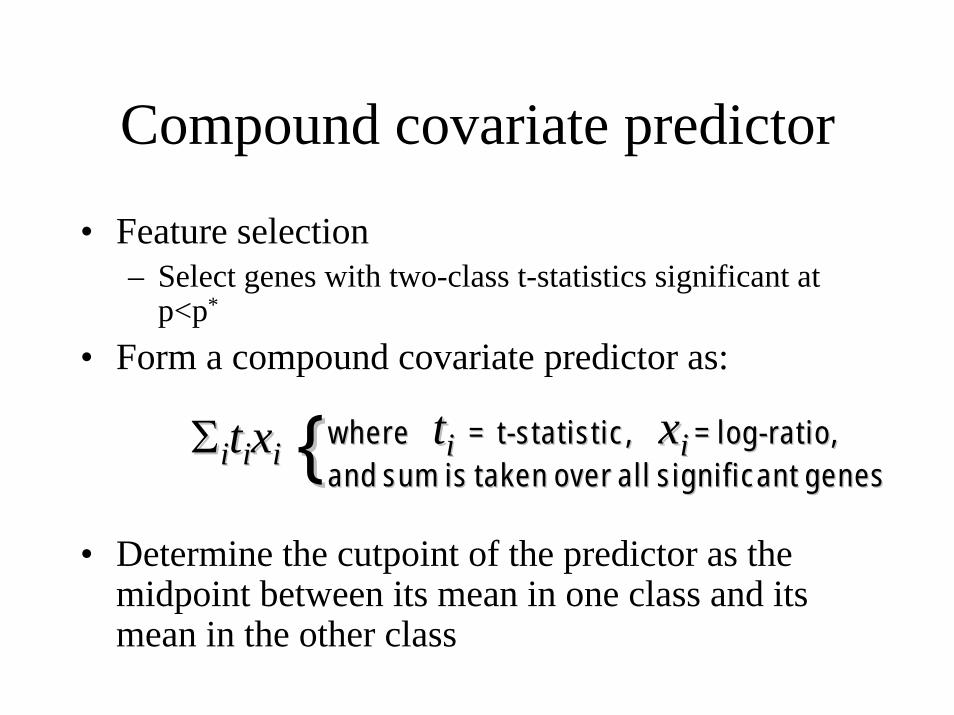
Compound covariate predictor
• Feature selection– Select genes with two-class t-statistics significant at
p<p*
• Form a compound covariate predictor as:
• Determine the cutpoint of the predictor as the midpoint between its mean in one class and its mean in the other class
ΣΣiittiixxii { where where ttii = t= t--statistic, statistic, xxii = log= log--ratio,ratio,and sum is taken over all significant genesand sum is taken over all significant genes{
Advantages of Compound Covariate Classifier
• Does not over-fit data– Incorporates influence of multiple variables
without attempting to select the best small subset of variables
– Does not attempt to model the multivariate interactions among the predictors and outcome
– A one-dimensional classifier with contributions from variables correlated with outcome
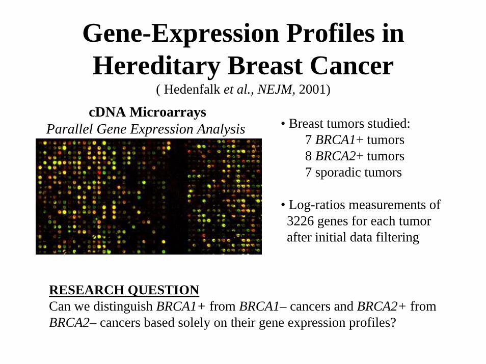
Gene-Expression Profiles in Hereditary Breast Cancer
( Hedenfalk et al., NEJM, 2001)
• Breast tumors studied:7 BRCA1+ tumors8 BRCA2+ tumors7 sporadic tumors
• Log-ratios measurements of 3226 genes for each tumor after initial data filtering
cDNA MicroarraysParallel Gene Expression Analysis
RESEARCH QUESTIONCan we distinguish BRCA1+ from BRCA1– cancers and BRCA2+ from BRCA2– cancers based solely on their gene expression profiles?
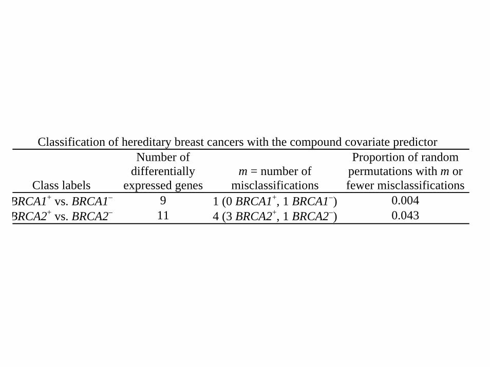
Classification of hereditary breast cancers with the compound covariate predictor
Class labels
Number ofdifferentially
expressed genesm = number of
misclassifications
Proportion of randompermutations with m orfewer misclassifications
BRCA1+ vs. BRCA1− 9 1 (0 BRCA1+, 1 BRCA1−) 0.004BRCA2+ vs. BRCA2− 11 4 (3 BRCA2+, 1 BRCA2−) 0.043

BRCA1
αg # of significantgenes
m = # of misclassified elements(misclassified samples)
% of randompermutations with m
or fewermisclassifications
10-2 182 3 (s13714, s14510, s14321) 0.410-3 53 2 (s14510, s14321) 1.010-4 9 1 (s14321) 0.2
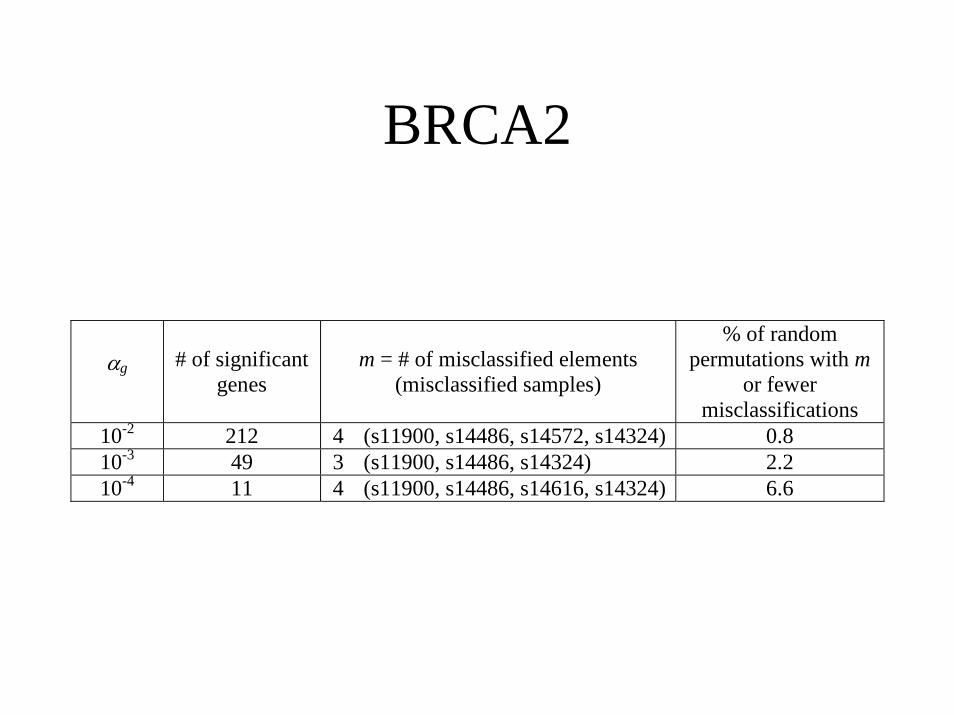
BRCA2
αg # of significantgenes
m = # of misclassified elements(misclassified samples)
% of randompermutations with m
or fewermisclassifications
10-2 212 4 (s11900, s14486, s14572, s14324) 0.810-3 49 3 (s11900, s14486, s14324) 2.210-4 11 4 (s11900, s14486, s14616, s14324) 6.6
Permutation Distribution of Cross-validated Misclassification Rate of a
Multivariate Classifier• Randomly permute class labels and repeat
the entire cross-validation• Re-do for all (or 1000) random
permutations of class labels• Permutation p value is fraction of random
permutations that gave as few misclassifications as e in the real data
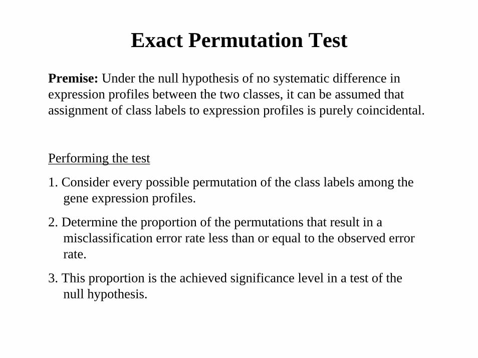
Exact Permutation Test
Premise: Under the null hypothesis of no systematic difference in expression profiles between the two classes, it can be assumed that assignment of class labels to expression profiles is purely coincidental.
Performing the test
1. Consider every possible permutation of the class labels among the gene expression profiles.
2. Determine the proportion of the permutations that result in amisclassification error rate less than or equal to the observed error rate.
3. This proportion is the achieved significance level in a test of thenull hypothesis.
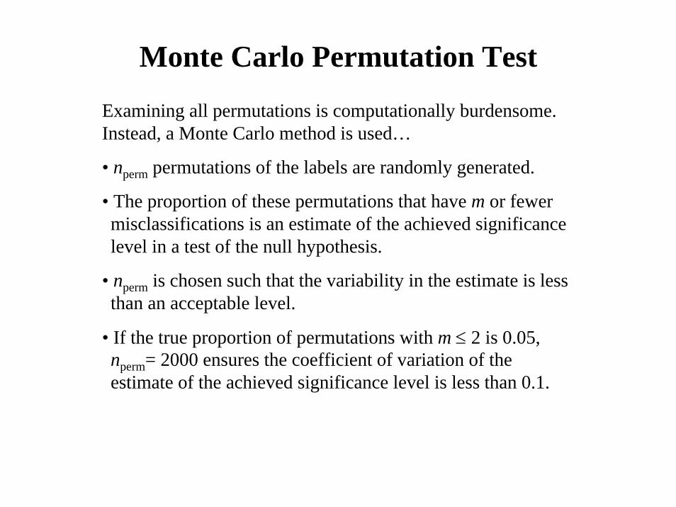
Monte Carlo Permutation Test
Examining all permutations is computationally burdensome.Instead, a Monte Carlo method is used…
• nperm permutations of the labels are randomly generated.
• The proportion of these permutations that have m or fewer misclassifications is an estimate of the achieved significance level in a test of the null hypothesis.
• nperm is chosen such that the variability in the estimate is less than an acceptable level.
• If the true proportion of permutations with m ≤ 2 is 0.05, nperm= 2000 ensures the coefficient of variation of the estimate of the achieved significance level is less than 0.1.

Distribution of the Number of Misclassificationsfor a Simulated Data Set
number of misclassifications
0 2 4 6 8 10 12 14
prob
abilit
y
0.00
0.05
0.10
0.15
0.20
0.25Binomial (n=14, p=0.5) Permutation

Compound Covariate Classification of DLCL Data. (GCC vs Activated B)
42 Samples, 2317 GenesNominal alpha Number of
DEGsNumber of
misclassificationsPermutational p
value0.01 275 3 0.00
0.001 97 5 0.00
0.0001 39 4 0.00
0.00001 16 4 0.00
0.000001 3 7 0.01
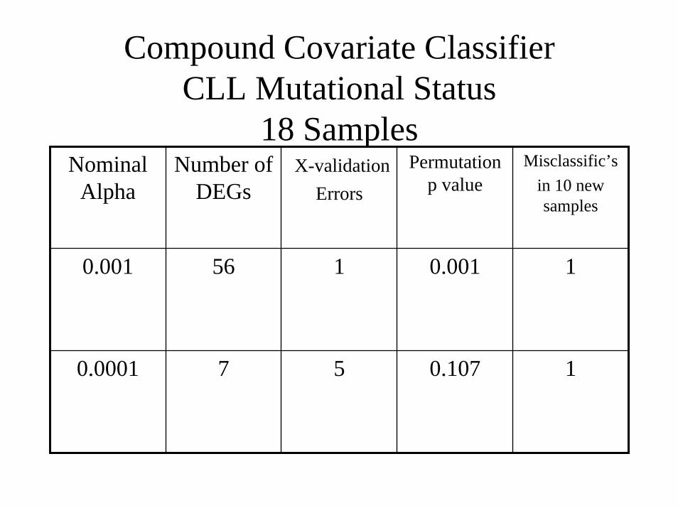
Compound Covariate ClassifierCLL Mutational Status
18 SamplesNominal
AlphaNumber of
DEGsX-validation
Errors
Permutation p value
Misclassific’sin 10 new samples
0.001 56 1 0.001 1
0.0001 7 5 0.107 1
Quadratic Discriminant Analysis
• Assumes that log-ratios (log intensities) have a multi-variate Gaussian distribution.
• The two classes have different mean vectors and potentially different covariance matrices.
• Using the training data, estimate the mean vector and covariance matrix for each class.
Quadratic Discriminant Analysis
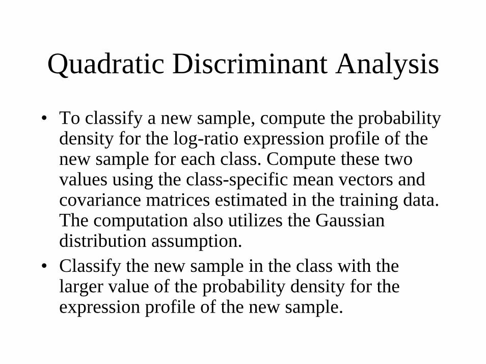
• To classify a new sample, compute the probability density for the log-ratio expression profile of the new sample for each class. Compute these two values using the class-specific mean vectors and covariance matrices estimated in the training data. The computation also utilizes the Gaussian distribution assumption.
• Classify the new sample in the class with the larger value of the probability density for the expression profile of the new sample.

Quadratic Discriminant Analysis
• With G genes in the model, there are G components of the mean vector to be estimated for each class and G(G+1)/2 components of the covariance matrix for each class. Hence a total of G(G+3) parameters to be estimated.
• With N samples, one has only NG pieces of data.

Diagonal Linear DiscriminantAnalysis
• Full QDA performs poorly when G >N. One can help somewhat by selecting the G genes to include based on univariate discrimination power.
• The number of parameters can be dramatically reduced by assuming that the variances are the same in the two classes and that covariance among genes can be ignored. This reduces the number of parameters to 3G. This is DLDA. It has performed as well as much more complex methods in comparisons conducted by Dudoit et al.
Diagonal Linear DiscriminantAnalysis
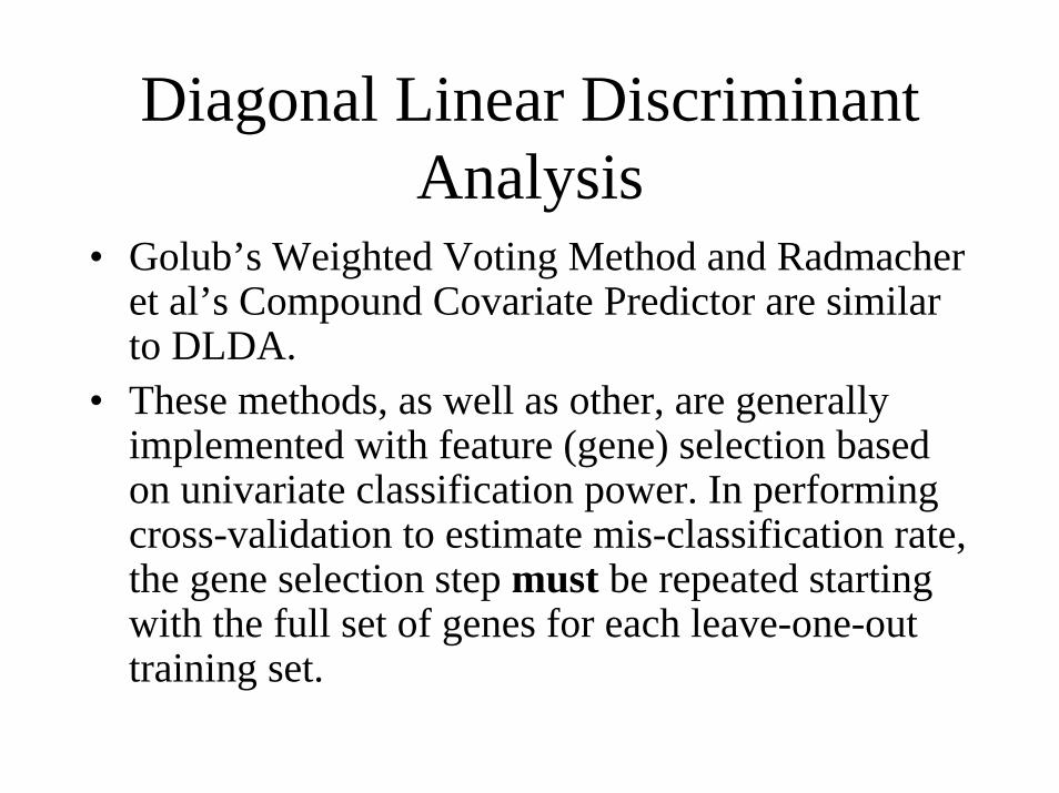
• Golub’s Weighted Voting Method and Radmacher et al’s Compound Covariate Predictor are similar to DLDA.
• These methods, as well as other, are generally implemented with feature (gene) selection based on univariate classification power. In performing cross-validation to estimate mis-classification rate, the gene selection step must be repeated starting with the full set of genes for each leave-one-out training set.

Neural Network Classification Kahn et al. Nature Med. 2001
• Not really a neural network (fortunately).• A perceptron with no hidden nodes and a linear
transfer function at each node.• Inputs are first 10 principal components
– The linear combinations of the genes that have greatest variation among samples and are orthogonal
• The method is essentially equivalent to DLDA based on the 10 PC’s as predictors
• They didn’t cross-validate the computation of the 10 PC’s.
Linear Classifiers for Two Classes
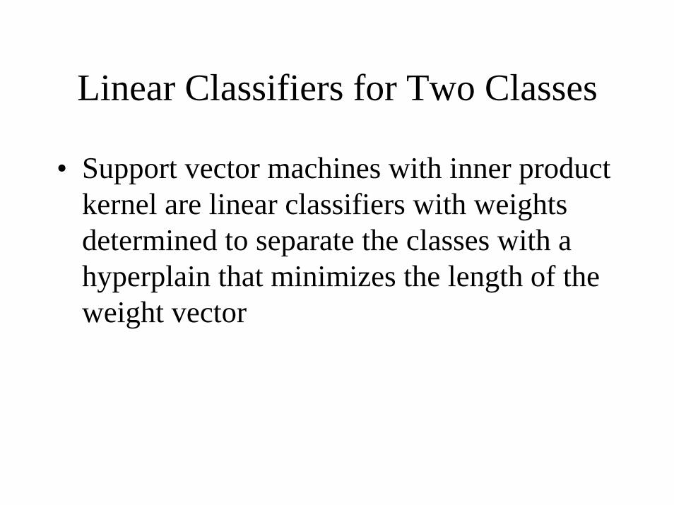
• Support vector machines with inner product kernel are linear classifiers with weights determined to separate the classes with a hyperplain that minimizes the length of the weight vector
Support Vector Machine
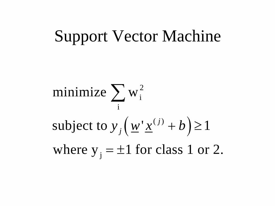
( )
2i
i
( )
j
minimize w
subject to ' 1
where y 1 for class 1 or 2.
jjy w x b+ ≥
= ±
∑
Compound Covariate BayesClassifier
• Compound covariate y = Σtixi– Sum over the genes selected as differentially expressed– xi the expression level of the ith selected gene for the
case whose class is to be predicted– ti the t statistic for testing differential expression for the
i’th gene• Proceed as for the naïve Bayes classifier but using
the single compound covariate as predictive variable– GW Wright et al. PNAS 2005.

Other Simple Methods
• Nearest neighbor classification• Nearest k-neighbors• Nearest centroid classification• Shrunken centroid classification
Nearest Neighbor Classifier• To classify a sample in the validation set as being
in outcome class 1 or outcome class 2, determine which sample in the training set it’s gene expression profile is most similar to.– Similarity measure used is based on genes selected as
being univariately differentially expressed between the classes
– Correlation similarity or Euclidean distance generally used
• Classify the sample as being in the same class as it’s nearest neighbor in the training set
K-Nearest Neighbor Classifier
• Find the k samples that are most similar to the sample to be classified
• Identify the majority class among the k nearest neighbor samples
• Classify the unknown sample as being in the majority class
Nearest Centroid Classifier• For a training set of data, select the genes that are
informative for distinguishing the classes• Compute the average expression profile (centroid) of the
informative genes in each class• Classify a sample in the validation set based on which
centroid in the training set it’s gene expression profile is most similar to.

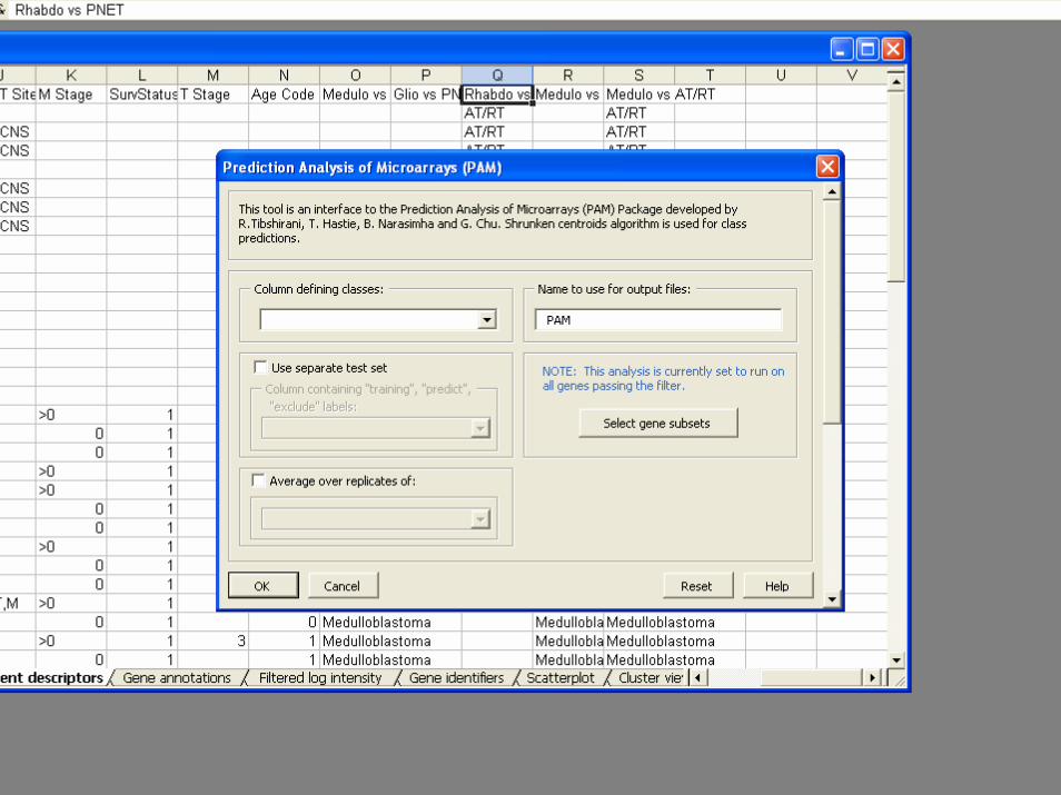
Nearest Shunken Centroids
i
i
1 1k
i
mean of gene i in class kcentroid vector of class meansx overall mean of gene i
x
standard deviation of gene i expression within each class
m
x(
k
ik
ik
k i
i
n n
ik k i ik
ik
x
xcm s
s
x m s dd sign d
=
==
−=
=
= +
′ ′= +
′ = { }) | |ik ikd+
−∆

Nearest Shunken CentroidsDiscriminant Score
( )
*
2**
k 2
expression profile of sample to be classified
( ) 2log
prior probability that sample is in class k
i ikk
i i
k
x
x xx
sδ π
π
=
′−= −
=
∑
Other Methods
• Top-scoring pairs– Claim that it gives accurate prediction with few
pairs because pairs of genes are selected to work well together
• Random Forrest– Very popular in machine learning community– Complex classifier
When There Are More Than 2 Classes
• Nearest neighbor type methods
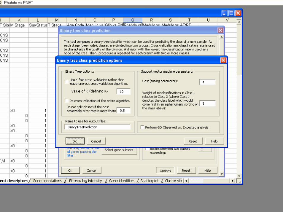
• Decision tree of binary classifiers
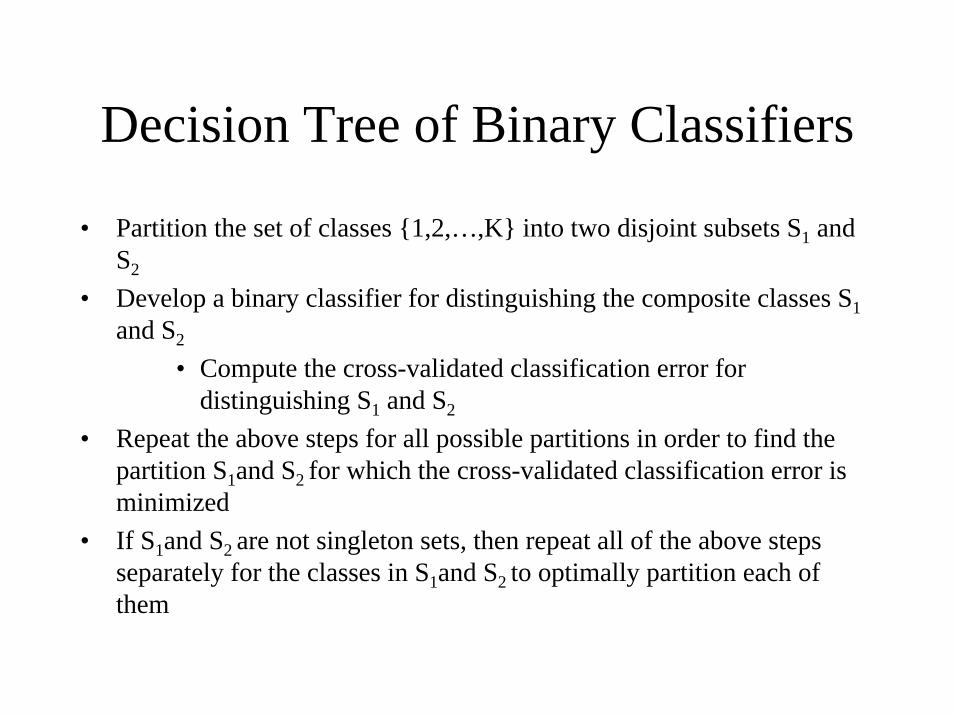
Decision Tree of Binary Classifiers
• Partition the set of classes {1,2,…,K} into two disjoint subsets S1 and S2
• Develop a binary classifier for distinguishing the composite classes S1and S2
• Compute the cross-validated classification error for distinguishing S1 and S2
• Repeat the above steps for all possible partitions in order to find the partition S1and S2 for which the cross-validated classification error is minimized
• If S1and S2 are not singleton sets, then repeat all of the above steps separately for the classes in S1and S2 to optimally partition each of them
Myth
• That complex classification algorithms such as neural networks perform better than simpler methods for class prediction.
Truth
• Artificial intelligence sells to journal reviewers and peers who cannot distinguish hype from substance when it comes to microarray data analysis.
• Comparative studies have shown that simpler methods work as well or better for microarray problems because the number of candidate predictors exceeds the number of samples by orders of magnitude.
When p>>n The Linear Model is Too Complex
• It is always possible to find a set of features and a weight vector for which the classification error on the training set is zero.
• Why consider more complex models?
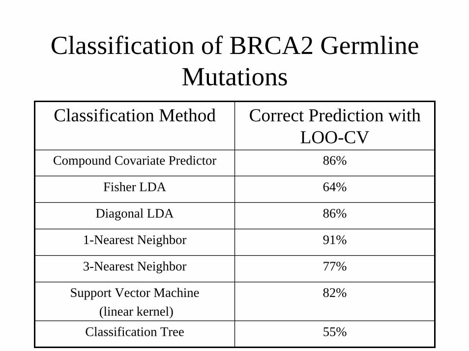
Classification of BRCA2 GermlineMutations
Classification Method Correct Prediction with LOO-CV
Compound Covariate Predictor 86%
Fisher LDA 64%
Diagonal LDA 86%
1-Nearest Neighbor 91%
3-Nearest Neighbor 77%
Support Vector Machine(linear kernel)
82%
Classification Tree 55%
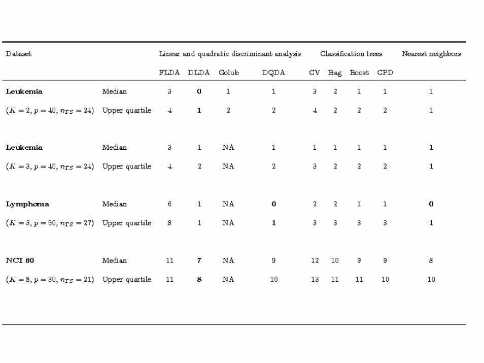
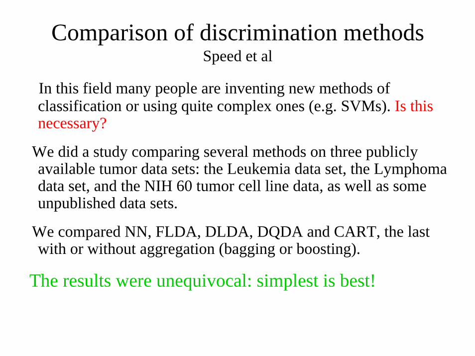
Comparison of discrimination methodsSpeed et al
In this field many people are inventing new methods of classification or using quite complex ones (e.g. SVMs). Is this necessary?
We did a study comparing several methods on three publicly available tumor data sets: the Leukemia data set, the Lymphoma data set, and the NIH 60 tumor cell line data, as well as some unpublished data sets.
We compared NN, FLDA, DLDA, DQDA and CART, the last with or without aggregation (bagging or boosting).
The results were unequivocal: simplest is best!
Approaches to Intra-study Validation
• Split data into training set and validation set– Validation set not accessed until proposed
classification system is fully specified based on training set
• Algorithmic cross-validation or bootstrap

Invalid Criticisms of Cross-Validation
• “You can always find a set of features that will provide perfect prediction for the training and test sets.”– For complex models, there may be many sets of
features that provide zero training errors. – A modeling strategy that either selects among
those sets or aggregates among those models, will have a generalization error which will be validly estimated by cross-validation.
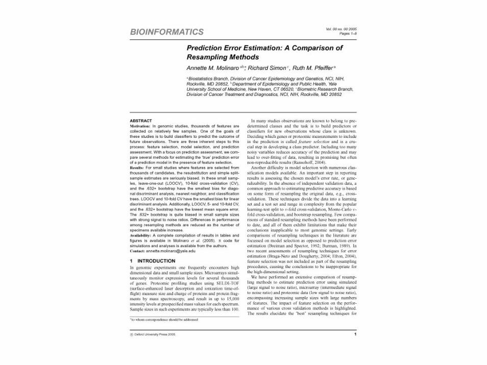

Simulated Data40 cases, 10 genes selected from 5000
Method Estimate Std DeviationTrue .078Resubstitution .007 .016LOOCV .092 .11510-fold CV .118 .1205-fold CV .161 .127Split sample 1-1 .345 .185Split sample 2-1 .205 .184.632+ bootstrap .274 .084

DLBCL DataMethod Bias Std Deviation MSE
LOOCV -.019 .072 .008
10-fold CV -.007 .063 .006
5-fold CV .004 .07 .007
Split 1-1 .037 .117 .018
Split 2-1 .001 .119 .017
.632+ bootstrap -.006 .049 .004
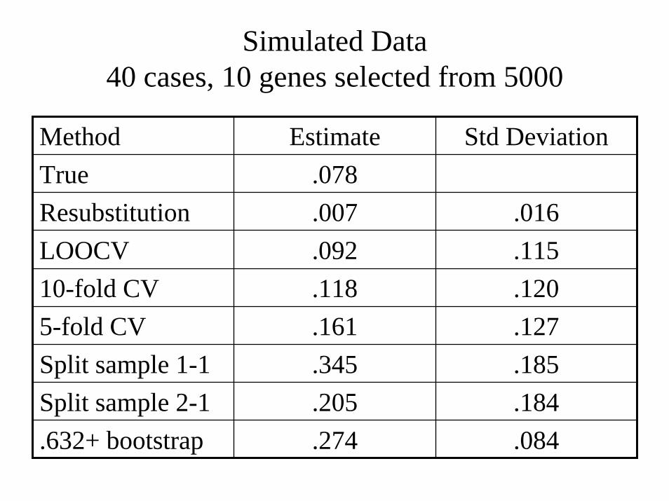
Simulated Data40 cases
Method Estimate Std DeviationTrue .07810-fold .118 .120Repeated 10-fold .116 .1095-fold .161 .127Repeated 5-fold .159 .114Split 1-1 .345 .185Repeated split 1-1 .371 .065

Common Problems With Internal Classifier Validation
• Pre-selection of genes using entire dataset
• Failure to consider optimization of tuning parameter part of classification algorithm– Varma & Simon, BMC Bioinformatics 2006
• Erroneous use of predicted class in regression model

Incomplete (incorrect) Cross-Validation
• Let M(b,D) denote a classification model developed on a set of data D where the model is of a particular type that is parameterized by a scalar b.
• Use cross-validation to estimate the classification error of M(b,D) for a grid of values of b; Err(b).
• Select the value of b* that minimizes Err(b).• Caution: Err(b*) is a biased estimate of the prediction error
of M(b*,D).• This error is made in some commonly used methods

Complete (correct) Cross-Validation
• Construct a learning set D as a subset of the full set S of cases.
• Use cross-validation restricted to D in order to estimate the classification error of M(b,D) for a grid of values of b; Err(b).
• Select the value of b* that minimizes Err(b).• Use the mode M(b*,D) to predict for the cases in S but not
in D (S-D) and compute the error rate in S-D• Repeat this full procedure for different learning sets D1 , D2
and average the error rates of the models M(bi*,Di) over the corresponding validation sets S-Di
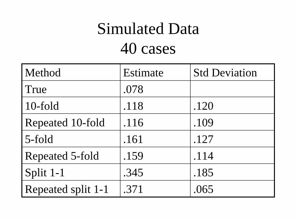
Does an Expression Profile Classifier Predict More Accurately Than Standard Prognostic
Variables?
• Not an issue of which variables are significant after adjusting for which others or which are independent predictors– Predictive accuracy and inference are different
• The two classifiers can be compared with regard to predictive accuracy
• The predictiveness of the expression profile classifier can be evaluated within levels of the classifier based on standard prognostic variables

Does an Expression Profile Classifier Predict More Accurately Than Standard Prognostic
Variables?
• Some publications fit logistic model to standard covariates and the cross-validated predictions of expression profile classifiers
• This is valid only with split-sample analysis because the cross-validated predictions are not independent
log ( ) ( | )i iit p y x i zα β γ= + − +
External Validation
• Should address clinical utility, not just predictive accuracy– Therapeutic relevance
• Should incorporate all sources of variability likely to be seen in broad clinical application– Expression profile assay distributed over time and
space– Real world tissue handling– Patients selected from different centers than those used
for developing the classifier
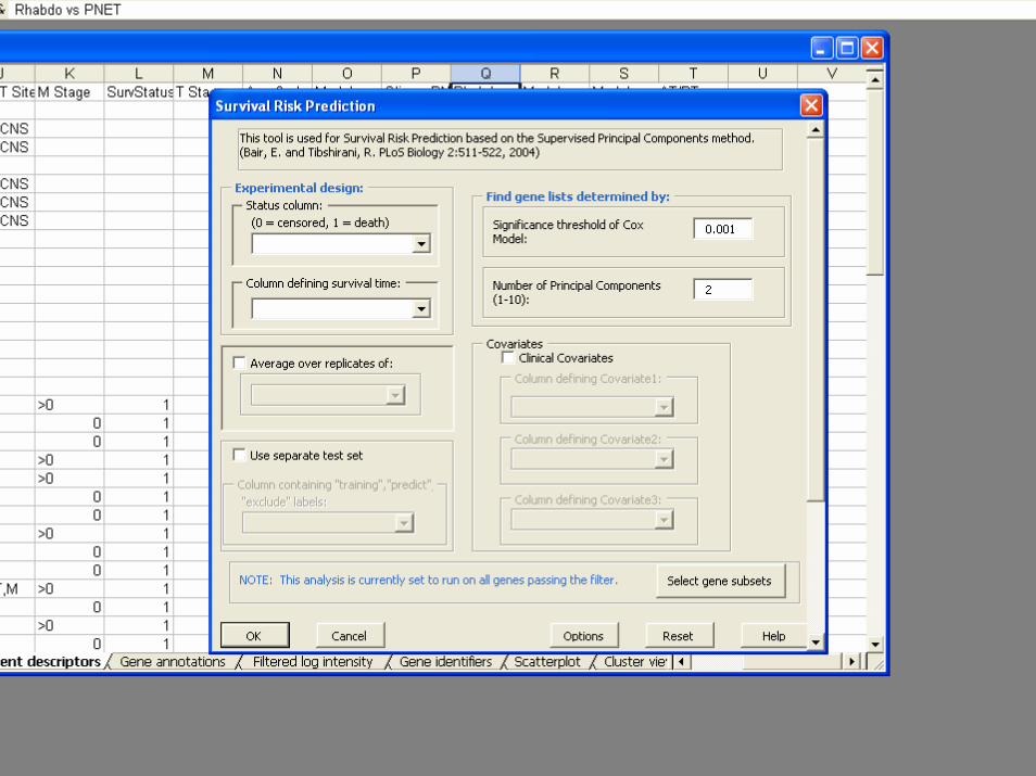
Survival Risk Group Prediction• Evaluate individual genes by fitting single variable
proportional hazards regression models to log signal or log ratio for gene
• Select genes based on p-value threshold for single gene PH regressions
• Compute first k principal components of the selected genes• Fit PH regression model with the k pc’s as predictors. Let
b1 , …, bk denote the estimated regression coefficients• To predict for case with expression profile vector x,
compute the k supervised pc’s y1 , …, yk and the predictive index λ = b1 y1 + … + bk yk
Survival Risk Group Prediction
• LOOCV loop:– Create training set by omitting i’th case
• Develop supervised pc PH model for training set• Compute cross-validated predictive index for i’th
case using PH model developed for training set• Compute predictive risk percentile of predictive
index for i’th case among predictive indices for cases in the training set
Survival Risk Group Prediction
• Plot Kaplan Meier survival curves for cases with cross-validated risk percentiles above 50% and for cases with cross-validated risk percentiles below 50%– Or for however many risk groups and
thresholds is desired• Compute log-rank statistic comparing the
cross-validated Kaplan Meier curves
Survival Risk Group Prediction
• Repeat the entire procedure for all (or large number) of permutations of survival times and censoring indicators to generate the null distribution of the log-rank statistic– The usual chi-square null distribution is not valid
because the cross-validated risk percentiles are correlated among cases
• Evaluate statistical significance of the association of survival and expression profiles by referring the log-rank statistic for the unpermuted data to the permutation null distribution
Survival Risk Group Prediction
• Other approaches to survival risk group prediction have been published
• The supervised pc method is implemented in BRB-ArrayTools
• BRB-ArrayTools also provides for comparing the risk group classifier based on expression profiles to one based on standard covariates and one based on a combination of both types of variables
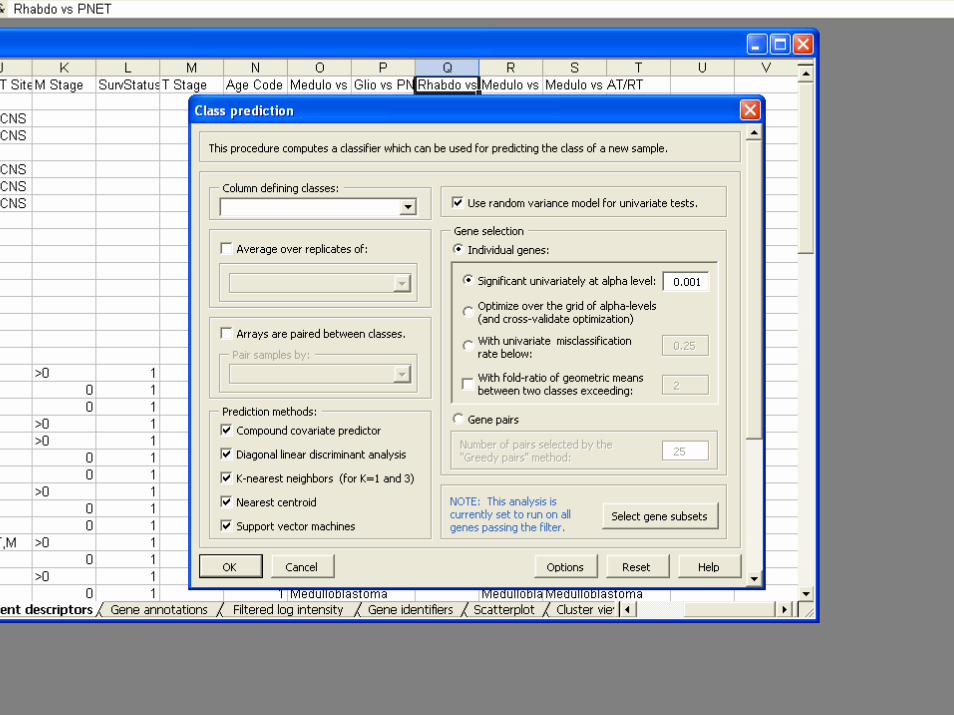
BRB-ArrayToolsClass Prediction
• Classifiers– Compound covariate predictor– Diagonal LDA– K-Nearest Neighbor Classification– Nearest Centroid– Support Vector Machines– Random Forest Classifier– Shrunken Centroids (PAM)– Top Scoring Pairs– Binary Tree Classifier

BRB-ArrayToolsClass Prediction
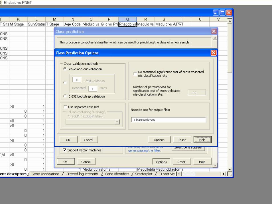
• Validation– Split Sample– Leave one out cross validation– K-fold cross validation– Repeated K-fold cross validation– .632+ Bootstrap resampling

BRB-ArrayToolsClass Prediction
• Gene Selection– Re-done for each re-sampled training set– Univariate significance level less than specified
threshold• Option for threshold for gene selection optimized by
inner loop of cross-validation
– Pairs of genes that work well together– Shrunken centroids
BRB-ArrayToolsClass Prediction
• Permutation test of significance of cross-validated misclassification rate
• Predictions for new patients
BRB-ArrayToolsSurvival Risk Group Prediction
• No need to transform data to good vs bad outcome. Censored survival is directly analyzed
• Gene selection based on significance in univariateCox Proportional Hazards regression
• Uses k principal components of selected genes• Gene selection re-done for each resampled
training set• Develop k-variable Cox PH model for each leave-
one-out training set

BRB-ArrayToolsSurvival Risk Group Prediction
• Classify left out sample as above or below median risk based on model not involving that sample
• Repeat, leaving out 1 sample at a time to obtain cross-validated risk group predictions for all cases
• Compute Kaplan-Meier survival curves of the two predicted risk groups
• Permutation analysis to evaluate statistical significance of separation of K-M curves
BRB-ArrayToolsSurvival Risk Group Prediction
• Compare Kaplan-Meier curves for gene expression based classifier to that for standard clinical classifier
• Develop classifier using standard clinical staging plus genes that add to standard staging


Class Prediction
• Cluster analysis is frequently used in publications for class prediction in a misleading way

Fallacy of Clustering Classes Based on Selected Genes
• Even for arrays randomly distributed between classes, genes will be found that are “significantly” differentially expressed
• With 10,000 genes measured, about 500 false positives will be differentially expressed with p < 0.05
• Arrays in the two classes will necessarily cluster separately when using a distance measure based on genes selected to distinguish the classes

Class Discovery
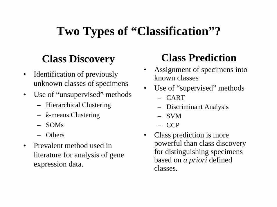
Two Types of “Classification”?
Class Discovery• Identification of previously
unknown classes of specimens• Use of “unsupervised” methods
– Hierarchical Clustering– k-means Clustering– SOMs– Others
• Prevalent method used in literature for analysis of gene expression data.
Class Prediction• Assignment of specimens into
known classes• Use of “supervised” methods
– CART– Discriminant Analysis– SVM– CCP
• Class prediction is more powerful than class discovery for distinguishing specimens based on a priori defined classes.
Class Discovery
• For determining whether a set of samples (eg tumors) is homogeneous with regard to expression profile
• To identify set of co-expressed, and perhaps co-regulated genes
Class Discovery of Samples
• Complex diseases often represent umbrella diagnoses and that heterogeneity limits the power of linkage and association studies
• Treatment selection and therapeutics development may be enhanced by biologically meaningful classification

Cluster Analysis
• Distance measure– Euclidean distance– Mahalanobis distance– 1- correlation– Mutual information– Bayes factor
• Feature (gene) set– All– Variably expressed– Selected to optimize
clustering
• Algorithm– Hierarchical – K means– Self Organized Map– Generative Topographical
Map– Autoclass– Bioclust– Gene shaving– Plaid– Splash– BiClustering

Clustering and Classification
• Analysis performed on log-ratios with two channel arrays
• Analysis performed on log signal values for GeneChips

Hierarchical AgglomerativeClustering Algorithm
• Merge two closest observations into a cluster.– How is distance between individual observations
measured?
• Continue merging closest clusters/observations.– How is distance between clusters measured?
• Average linkage• Complete linkage• Single linkage
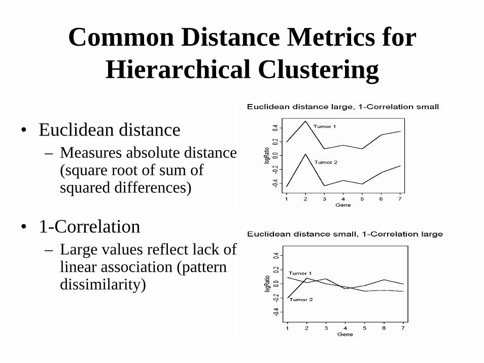
Common Distance Metrics forHierarchical Clustering
• Euclidean distance– Measures absolute distance
(square root of sum of squared differences)
• 1-Correlation– Large values reflect lack of
linear association (pattern dissimilarity)
Linkage Metrics• Average linkage
– Distance between clusters is average of all pair-wise distances between members of the two clusters
• Complete linkage– Distance is maximum of pair-wise distances– Tends to produce compact clusters
• Single linkage– Distance is minimum of pair-wise distances– Prone to “chaining” and sensitive to noise
• Centroid/Eisen linkage– Distance is the distance between the centroids of the two clusters

1 2 34
56
7 89
1011
12 1314
15 1617
1819 20
2122
23 2425
26 2728 29
30 31
0.2
0.3
0.4
0.5
0.6
0.7
0.8
Clustering of Melanoma Tumors Using Average Linkage
1 2 3
4
5
6
7 8
910
1112 13
1415 16
17 1819 20
21
2223 24
25
26 27
28 29
30 31
0.2
0.4
0.6
0.8
1.0
Clustering of Melanoma Tumors Using Complete Linkage
1 2 3
4
5
6
7
8
910
1112 13
14
15 16
17 1819 20
21
2223 24
25
26
27
28 29
30
31
0.2
0.3
0.4
0.5
0.6
Clustering of Melanoma Tumors Using Single Linkage
Dendrograms using 3 different linkage methods, distance = 1-correlation
(Data from Bittner et al., Nature, 2000)
Gene Centering
• Subtracting overall average value for each gene• Does not influence Euclidean distance between
samples• Does influence correlation between samples
– Reduces influence of genes whose expression in internal reference is very different than in samples
– Beneficial for clustering samples when internal reference is arbitrary
Gene Standardization
• Dividing gene expression by standard deviation or maximum value for that gene
• Useful for single channel data to reduce the influence of high intensity genes
• Not useful for two channel data because it amplifies noise for non-informative genes
0.0
0.1
0.2
0.3
0.4
0.5
0.6
1-co
rrel
atio
n
17
13
19
18
1514 16
12
11
20
2
6
8 9
7 10
3
4
5
1
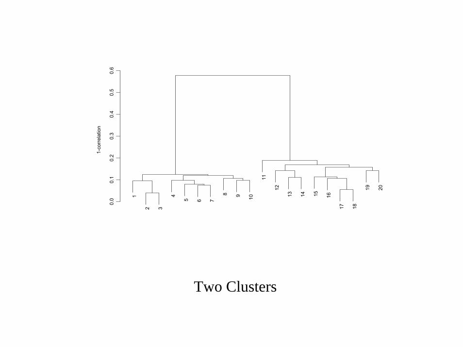
Two Clusters
0.8
1.0
1.2
1-co
rrel
atio
n
13
2
17
3
15 16
19
1
9
4
7
14
20
5 18
8
11
10
6
12
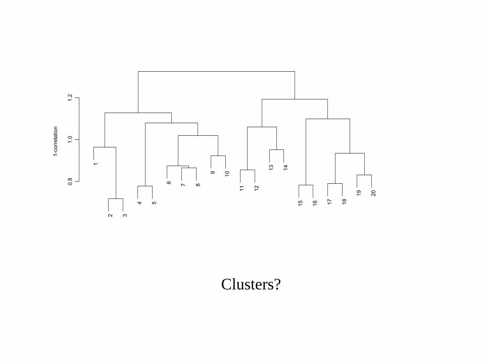
Clusters?
Genes Used for Clustering
• Samples may cluster differently with regard to different gene sets
• All genes• All “well measured” genes
– Genes with fewer than specified percentage of values filtered because of low intensity or poor imaging
• Genes with most variation across samples
Measures of Gene Expression Variability
• Proportion of arrays in which the gene is two-fold different from it’s mean or median value
• Variance of gene expression across the arrays (Vi) – In the upper k’th percentile of variance for all
genes– Is statistically significantly greater than the
median variance for all genes
Genes Used for Clustering Samples
• Genes selected as being differentially expressed between pre-defined classes– The cluster dendrogram is a visual display that
the samples are distinct with regard to these genes, but it is not independent evidence of the biological relevance of the genes
Fallacy of Clustering Classes Based on Selected Genes
• Even for arrays randomly distributed between classes, genes will be found that are “significantly” differentially expressed
• With 8000 genes measured, 400 false positives will be differentially expressed with p < 0.05
• Arrays in the two classes will necessarily cluster separately when using a distance measure based on genes selected to distinguish the classes
Clustering Algorithms
• K-means– Pre-specify K. – Initialize with a center for each cluster– Grow each cluster by adding unassigned
elements (samples or genes) to the cluster center they are nearest
– Redefine cluster centers as clusters grow and permit elements to shift clusters
– Various implementations and variants
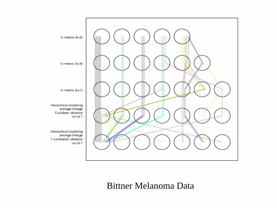
Bittner Melanoma Data
Self Organizing MapsSOM’s
• Often described in the language of artificial and natural neural networks but really just a clustering algorithm
• A spatially smooth version of K-means with large K• Cluster centers are computationally determined so that the
distances among centers corresponds to the distances among points arranged in a regular 2-d or 3-d lattice. Each cluster center projects to a single lattice point.
• Clusters corresponding to adjacent lattice points are similar giving a continuous variation appearance to the clusters
• Can be useful for clustering genes using time series data

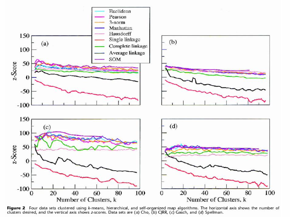
Validation of Clusters
• Clustering algorithms find clusters, even when they are spurious
• Clusters found may change with re-assaying tumors or selection of new tumors
Clustering Arrays
• Cluster significance• Cluster reproducibility

Cluster SignificanceMcShane et al
• Transform expression data to 3-d principal component space
• Compute median of empirical distribution of distance of each sample from its nearest neighbor
• Compute distribution of above statistic for data generated from multivariate Gaussian null distribution in principal component space
• Repeat for 1000 samples from the Gaussian null distribution
Cluster Significance
• Determine the proportion of the null distribution replications that the median of nearest neighbor distances is as small as for the median of nearest neighbor distances with the actual data
Assessing Cluster Reproducibility:Data Perturbation Methods
• Most believable clusters are those that persist given small perturbations of the data.
– Perturbations represent an anticipated level of noise in gene expression measurements.
– Perturbed data sets are generated by adding random errors to each original data point.
• McShane et al. Gaussian errors• Kerr and Churchill (PNAS, 2001) – Bootstrap residual errors
Assessing Cluster Reproducibility:Data Perturbation Methods
• Perturb the log-gene measurements and re-cluster.
• For each original cluster:– Compute the proportion of elements that occur together in the
original cluster and remain together in the perturbed data clustering when cutting dendrogram at the same level k. D-index.
– Average the cluster-specific proportions over many perturbed data sets to get an R-index for each cluster.

Discrepancy Index
k = 3
c1 c2 c3
Perturbed Data3) Perturb data by adding random Gaussian noise to each data point.
4) Perform clustering and cut into a similar number of clusters as original data.
5) Map from each original cluster ci to the perturbed cluster that minimizes the sum of missing (m) elements.
p1 p2
}
p3= c1*
Original Data1) Perform clustering on data.
2) Cut at height that results in k clusters.
= c2* = c3
*

Discrepancy Index
p1 = c1*
}Original Data Perturbed Data
c1 c3c2 p2 p3= c2* = c3
*
k = 3
m(missing)
n(contaminating)
c1 → c1*: 1 1
c2 → c2*: 1 2
c3 → c3*: 1 0
( ) 63
1
=∑ +=′=i
iinmε
Compute minimal mn-error for this cut of original data:
ε′ can be averaged over many perturbations resulting in .ε ′

Melanoma Gene Expression Data0.
20.
30.
40.
50.
60.
70.
8
11
2
9
12
6
25
10
4
13
1 3
28
29
26
21
7
23
30
22
24
8
31
18
27
5
17
19
20
14
15
16
1 -c
orre
latio
n
19 tumor cluster of interest
Q: Can gene expression profiles of melanoma be used to distinguishsub-classes of disease? (M. Bittner et al.)
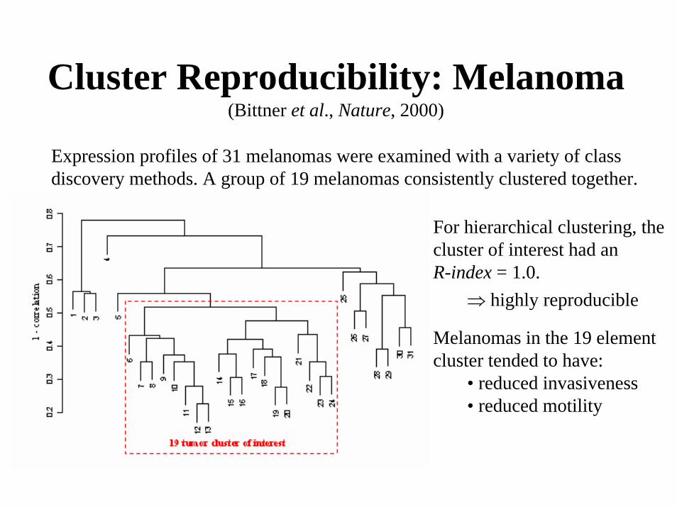
Cluster Reproducibility: Melanoma(Bittner et al., Nature, 2000)
Expression profiles of 31 melanomas were examined with a variety of class discovery methods. A group of 19 melanomas consistently clustered together.
For hierarchical clustering, the cluster of interest had an R-index = 1.0.
⇒ highly reproducible
Melanomas in the 19 element cluster tended to have:
• reduced invasiveness• reduced motility

Melanoma Data:Discrepancy Index - Individual Clusters
kCluster
Membership m ′ n ′7 5-24 0.00 0.00
8 5 0.00 5.13
8 6-24 0.00 0.27
0.2
0.3
0.4
0.5
0.6
0.7
0.8
11
2
9
12
6
25
10
4
13
1 3
28
29
26
21
7
23
30
22
24
8
31
18
27
5
17
19
20
14
15
16

Visualization Tools
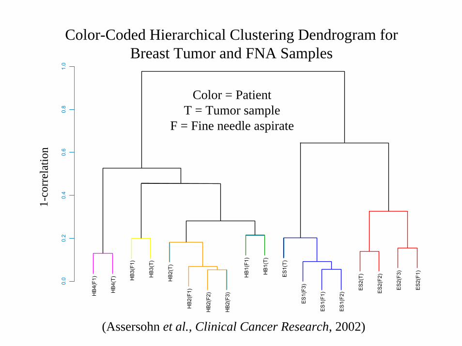
0.0
0.2
0.4
0.6
0.8
1.0
HB
1(F1
)
HB
1(T)
HB
2(T)
HB
2(F1
)
HB
2(F2
)
HB
2(F3
)
HB
3(F1
)
HB
3(T)
ES
2(F3
)
ES
2(T)
HB
4(F1
)
HB
4(T)
ES
1(F1
)
ES
1(F2
)
ES
1(F3
)
ES
1(T)
ES
2(F1
)
ES
2(F2
)
Color-Coded Hierarchical Clustering Dendrogram forBreast Tumor and FNA Samples
1-co
rrel
ati o
n
Color = PatientT = Tumor sample
F = Fine needle aspirate
(Assersohn et al., Clinical Cancer Research, 2002)
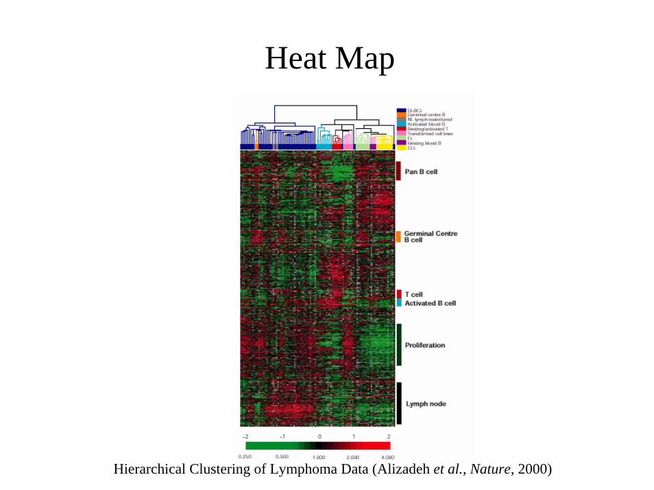
Heat Map
Hierarchical Clustering of Lymphoma Data (Alizadeh et al., Nature, 2000)
Multidimensional Scaling
• How to most accurately represent the pairwisedistances between expression profiles (vector of log-ratios or vector of log intensities) in 5000-d space in a 3-dimensional plot– Pair-wise distance relationships cannot be exactly
represented in low dimension– MDS gives a best approximation– The first three principal components are approximately
optimal for 3-d representation
Principal Components for Representing Samples
• The first principal component is the linear combination of gene expression levels that has the greatest variation among all linear combinations – xi denotes the log-ratio for the i’th gene– Linear combination = a1x1+…+ anxn
– Where a12 + … + an
2 = 1
Principal Components for Representing Samples
• The second principal component is the linear combination of gene expression levels that shows the largest variation among all linear combinations orthogonal to the first principal component– Linear combination b1x1+…+ bnxn is
orthogonal if a1b1+…+ anbn =0
Principal Components for Representing Samples
• Principal components being linear combinations of genes are not easily interpretable in terms of which genes are highly represented
• Principal components can be very useful for visualizing distance relationships between samples where they capture much of the variation eventhough they may not be identified with specific genes
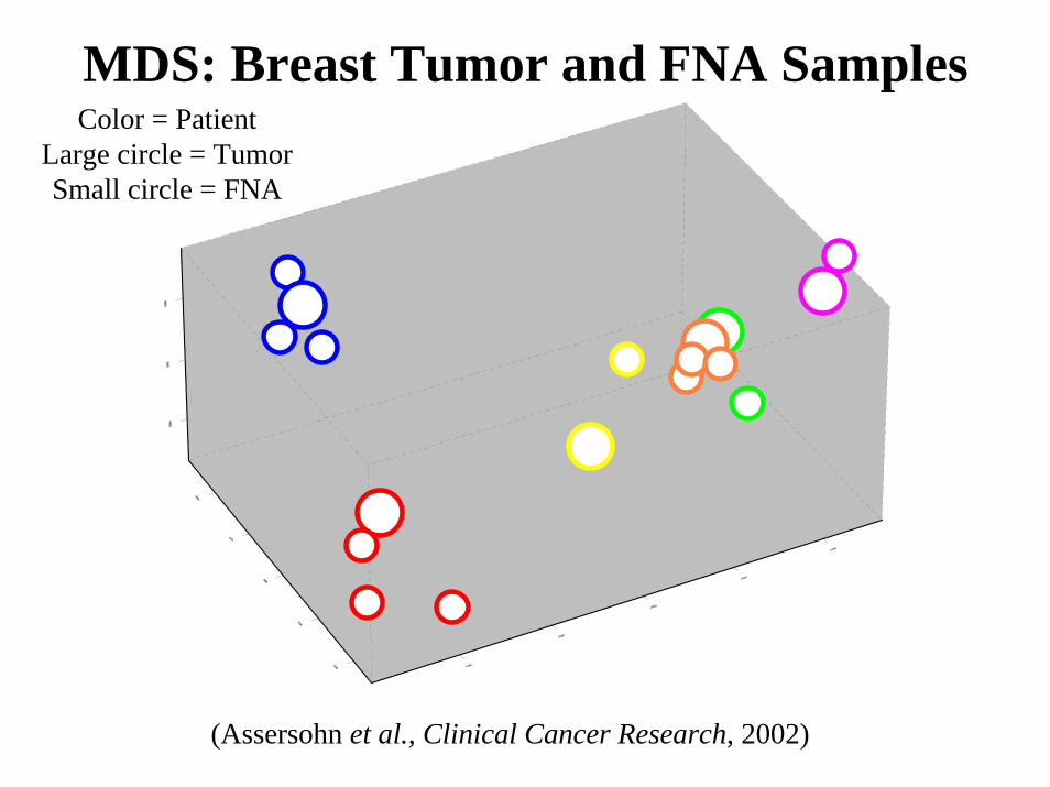
MDS: Breast Tumor and FNA Samples
(Assersohn et al., Clinical Cancer Research, 2002)
Color = PatientLarge circle = TumorSmall circle = FNA
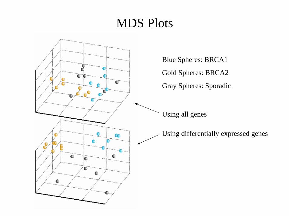
MDS Plots
Blue Spheres: BRCA1
Gold Spheres: BRCA2
Gray Spheres: Sporadic
Using all genes
Using differentially expressed genes
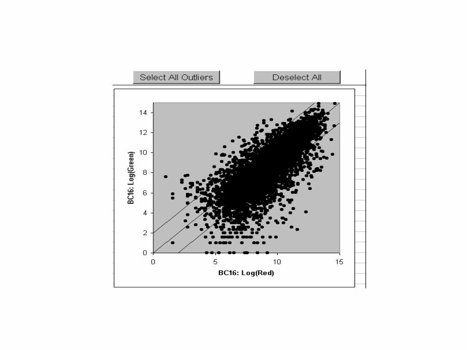
Scatterplots• Array vs array
– Log-ratio vs log-ratio or log signal vs log signal• MA for single array
– Mean of log red and log green intensities vs log-ratio• Scatterplot of phenotype averages
– Plots average log-ratio or log signal, averaged over classes of arrays
• Identification of outliers• Click on plots to hyperlink to clone reports• Double-click to view gene annotations (if
available)

Scatterplot of phenotype averagesPomeroy dataset