design & analysis of a distributed routing algorithm

Computer Communications 146 (2019) 201–218

Contents lists available at ScienceDirect

Computer Communications

journal homepage: www.elsevier.com/locate/comcom

Design & analysis of a distributed routing algorithm towards Internet-widegeocastBernd Meijerink a,∗, Mitra Baratchi b, Geert Heijenk a

a University of Twente, Enschede, The Netherlandsb Leiden Institute of Advanced Computer Science (LIACS), Leiden University, Leiden, The Netherlands

A R T I C L E I N F O

Keywords:GeocastRoutingGeographic routing

A B S T R A C T

Geocast is the concept of sending data packets to nodes in a specified geographical area instead of nodeswith a specific address. This forwarding method is valuable in situations where any number of nodes inside ageographic area need to be reached, such as vehicular networking scenarios. To facilitate large scale geocast, awired network geographic routing algorithm is needed that can route packets efficiently towards a destinationarea. Our goal is to design an algorithm that can deliver shortest path tree like geographic forwarding whilerelying purely on distributed data without central knowledge. In this paper we present and implement twoalgorithms for geographic routing. One algorithm is based purely on distance-vector data. Another, morecomplicated algorithm is based on path data. We show that our purely distance-vector-based algorithm cancome close to the number of links used by a shortest path tree when a small number of routers are presentin the destination area. We also show that our path-based algorithm can come close to the link usage of ashortest path tree in almost all geocast situations. We also show that the algorithms converge relatively quicklyfollowing link drops.

1. Introduction

Due to the increasing use of connected, possibly autonomous, vehi-cles and ‘smart’ devices there is an increasing need for Internet-wide ge-ographically scoped communications [1]. Geographically scoped com-munications, or geocast, would allow devices in a specific area to beaddressed without the need for tracking IP addresses or administrationconcerning multicast groups.

Geocast was first introduced by Navas and Imielinski [2]. It is atransmission method where packets are sent to a location or area ratherthan an IP-address. It can be seen as a one-to-many or many-to-manysystem like multicast with the main difference that devices receivepackets based on their location rather than a subscription model.

While geocast might seem similar to multicast in some ways,multicast-like routing will not be sufficient in a geocast environment forscalability reasons. Multicast routing algorithms are mostly designed toroute packets towards predefined multicast groups that are relativelystatic. Receivers also need to subscribe to specific groups, which canprove problematic in situations where either the sender(s) or receivershave a high rate of change. Geocast packets on the other hand will haveto be routed to a set of routers based on an sender-specified destinationarea that could contain several or even zero routers. The destination

∗ Corresponding author.E-mail addresses: [email protected] (B. Meijerink),

[email protected] (M. Baratchi), [email protected](G. Heijenk).

area can take any shape or size which in turn makes predefined areasproblematic.

Our work mostly focuses on the possible applications of geocast inthe vehicular network domain. Possible applications would be locationdependent weather updates, traffic alerts and information to assistautonomous driving. In the vehicular networking scenario a functioninggeocast solution would at least require location-aware base stations, orRoad Side Units (RSUs) that are aware of the area they serve. Locationaware-systems are important for many safety applications related tovehicular networks [3]. One example of a vehicular networking geocastscenario would be notifying cars on a specific highway of an accidentor traffic jam, using geocast to only send the message to that street.An example of such a situation is depicted in Fig. 1. A RSU forwardsa notification of a traffic accident to multiple vehicles on the roadthe accident took place on. Other examples would be a central trafficcontrol centre that needs to send messages to all vehicles in a specificarea, or a location-specific weather warning for road users in a specificregion.

Previous proposals for geographic routing are mostly applicationlayer based, an example being extended DNS [4]. There are two maindownsides to such an approach. They have high overhead due tolookup operations and are less resilient to change. We propose analternative approach to the problem: Implementing geocast on thenetwork layer. A network layer implementation would allow us to

https://doi.org/10.1016/j.comcom.2019.07.025Received 19 November 2018; Received in revised form 22 July 2019; Accepted 27 July 2019Available online 30 July 20190140-3664/© 2019 Published by Elsevier B.V.

https://doi.org/10.1016/j.comcom.2019.07.025

http://www.elsevier.com/locate/comcom

http://www.elsevier.com/locate/comcom

http://crossmark.crossref.org/dialog/?doi=10.1016/j.comcom.2019.07.025&domain=pdf

mailto:[email protected]



https://doi.org/10.1016/j.comcom.2019.07.025

B. Meijerink, M. Baratchi and G. Heijenk Computer Communications 146 (2019) 201–218

Fig. 1. Geocast traffic accident example.

use information already available due to unicast routing. The systemwould also be more resilient due to not relying on the availability ofcertain servers. Embedding geocast in the network itself will also allowit to route around problems in the network. It would also enable sucha system to possibly scale to the entire Internet. Enabling Internet-wide geocast could potentially allow fine grained geographically scopedmessage transmission for everyone. The main benefit would be thatsending hosts on the network do not require any sort of geographicalinformation, they can just send a geocast packet to the router servingthem. Possible use cases of network layer geocast range from local-ized weather reports without clients reporting their location to safetyinformation transmitted to vehicles.

To provide an efficient geocast solution, the underlying routing pro-tocol will need to take geographic information into account. Traditionalrouting methods such as unicast or multicast routing have drawbacksin the geocast scenario in that additional signalling or even over thetop solutions are needed to enable geographic routing. Unicast routinghas the obvious drawback of sending one packet per destination. Thiswould lead to communications overhead when a large number ofdevices is present in the destination area. On the other hand, theper-packet processing overhead is minimal as unicast routing is wellunderstood and optimized. Multicast routing seems like a better fit asit already supports one-to-many communications. The main drawbackfor geographically scoped communication is that most multicast rout-ing solutions depend on subscription messages. In a geocast solution,routers will need to report their coverage area and evaluate whichrouters cover the destination area of a packet. Another drawback wouldbe the requirement of predefined destination areas, as it would have tobe known which multicast group covers which area.

We set out to design a distributed algorithm, as the communicationoverhead needed for a centralized approach would lead to scalabilityproblems for the system. Routers should not depend on some central au-thority or need full network knowledge. This last requirement preventsus from constructing a least cost (Steiner) tree, as this would requirefull network knowledge. We will cover this last point in greater detailin Section 2.3.

For efficient geographic routing we need a routing algorithm inwhich geographical areas are central to packet routing. A geographicrouting algorithm will need to efficiently route packets that have ageographic destination to all routers that (partially) cover that area.We specifically refer to coverage instead ‘being in the area’, as theimportant thing is that devices connected to the router are in thedestination area. The most important aspect is the ability to routea packet to multiple destinations using the lowest number of hopspossible, without sending duplicate packets over the same link.

We use two area definitions in our geocast system: Coverage areaand destination area. Coverage Area defines the geographic area that iscovered by a router, devices in this area can be reached through thisrouter. Coverage areas of routers may overlap or even be identical, forexample multiple providers servicing the same area. Destination arearefers to the geographic area to which a packet is sent. This area doesnot need to be identical to the coverage area of a router, instead routersshould calculate if the destination overlaps with their coverage area.

Fig. 2. Area of interest. (For interpretation of the references to colour in this figurelegend, the reader is referred to the web version of this article.)

In this paper we specifically focus on routing between routers (asenclosed by the green rectangle in Fig. 2), we do not consider end-hosts.We consider the router that initially receives a packet as the source. Theactual source might be an end-host connected to that router or someother network. We consider a router a destination if the intersection ofone or more of its coverage areas and the destination area is not empty.A router’s coverage area (as enclosed by the blue rectangles in Fig. 2) isdefined by one or more rectangles that enclose all end-hosts connectedto the router and the area covered by all wireless access devices thatare connected to the router.

The main research question we answer in this paper is: How can weefficiently route geocast packets within a network? The main contribu-tion of our work is threefold:

• We design and implement a geographical routing algorithm usingpurely distance-vector based information,

• We design and implement an efficient geographical routing algo-rithm based on path information,

• We validate and evaluate the proposed algorithms and theirimplementation on a large set of real world network topologies,both in terms of link cost and convergence aspects.

Whereas the first routing algorithm mentioned above is very efficientwith respect to link cost, the second algorithm is computationally verysimple, at the cost of a somewhat higher link cost for the resultingdistribution tree and can be used in cases where network capacity isless important than router resources.

The remainder of this paper is structured as follows: In the nextsection we will describe previous work in the area, including our ownwork on geographic addressing. Section 3 will describe the algorithmswe have designed to perform geographic routing. We evaluate ouralgorithms in Section 4. In Section 5 we describe implementationsof our algorithms, of which we evaluate the convergence propertiesduring link loss in Section 6. Finally we draw our conclusions inSection 7.

2. Previous work

In this section, we will describe previous work done on geocastand geographic routing. We start with describing related work in thewireless domain, moving towards work on geocast in a wired setting.We will conclude the section with an overview of our own work ongeographic addressing and forwarding tree evaluation, in which we willexplain our choice for a shortest path tree.

2.1. Related work

Geocast was initially introduced by Navas and Imielinski for wirednetworks [2]. Their approach relied on special routers that know theirlocation and forward packets based on the destination point, circle or

202


polygon. Routers are connected hierarchically: A router that covers acertain area connects to ‘lower’ routers that cover smaller areas withinthat coverage area. Routers can calculate the intersect of destinationand their coverage using the GPS coordinates. Downsides of this ap-proach are the hierarchical router requirement, the need for routers toperform area intersection calculations and the variable length of theaddressing (points, circles, or polygons).

In later work from the same authors they studied improved rout-ing cost [5] by approximating the destination/coverage area intersec-tion. They have also studied alternate approaches based on addressingpredefined locations [6].

Most work on the topic of geocast has been done in the wirelessad-hoc network context, and especially the VANET case. Overviews ofsuch routing protocols and underlying mechanism can be found in [7,8]and [9]. In most of these protocols the location of forwarding nodes istightly coupled with the destination of a packet, a next hop node willgenerally be in the direction of the destination area. The correlationbetween the position of the next hop node and the location of thedestination area does not necessarily exist in a fixed wired networksituation. Especially in situations were a network serves several accessnetworks, there might be very little correlation between the forward-ing routers and the actual destination area. On the other hand, thefixed wired environment is usually mostly static, this enables routedistribution to be effective over long distances.

A well-known example of a geographic routing protocol for ad-hoc networks is GeoTORA [10]. When a node in the network needsto geocast a message it broadcasts a query with the request for thedestination nodes. The destination nodes send a message back, allowingthe original requesting node to know the forwarding hop towards thegeocast area. The mobile nature of these ad-hoc networks makes thiskind of signalling a necessity to reach any sort of efficiency. We donot have this problem in wired networks, allowing for the possibilityof route distribution beforehand.

Another example is Greedy Perimeter Stateless Routing [11]. Inthis algorithm, traffic is routed to nodes that are located closer to thedestination area than the transmitting node. This approach is seen oftenin geographic routing solutions for ad hoc networks. The downside fora wired environment is that the location of routers is not necessarilycorrelated with the direction a packet needs to travel to reach itsdestination.

An interesting grid based ad-hoc routing system is the Grid LocationService (GLS) [12]. This system has nodes keep track of each otherslocation in a distributed manner, where nodes closer to a node aremore likely to know its location. The geographic routing layer of GLSaddresses nodes based on their current location and uses a distance-vector protocol with two hop knowledge to route packets to theirdestination. This protocol allows nodes to lookup the location andsend packets to a specific other node. This requires the location of allpossible destinations to be knows somewhere in the network, while wewould like to address any number of nodes in a given area preferablywithout any knowledge (of the potentially large number) of nodes inthis area.

There are off-course algorithms for multicast routing such as Proto-col Independent Multicast (PIM). These could be used in some capacityfor geocast routing but they do have some drawbacks. PIM DenseMode (PIM-DM) relies on an initial flooding stage where routers thatare not subscribers send a prune message back to their forwardingneighbour [13]. We would ideally like to not have this behaviour inour geocast system as we believe the number of destination areas thatmight be addressed in a short time could be very large. Alternatively,PIM Sparse Mode (PIM-SM) relies on an initial Rendezvous Router thatroutes packets before a shortest path tree is established [14]. Due tothe large number of varying geocast destinations and the overheadcaused by the Rendezvous Router we believe this approach would notbe feasible.

Another, application layer, approach to geocast is to use DNS toresolve geographical areas to an IP addresses by extending the DNS [4].

Fig. 3. Geographic addressing up to level 3.

When the eDNS server is queried for a certain area, it returns theIP addresses of all entries in that region. The eDNS was designedfor VANET scenarios, so it would only have to return a list of RSUsin the target area. Scaling the system to track the movements of allvehicles to also allow geocasting from multiple networks at the sametime was later found to be somewhat feasible [15]. For a truly Internet-wide deployment such a system would need to scale significantly. DNSdelegation would also be complicated if updates are to be distributedthrough the network in a relatively short time.

2.2. Geographic addressing

The addressing system our routing system is based on is described inour previous work [16]. Our addressing scheme transforms a locationbounding box defined by its maximum and minimum latitude andlongitude into a format that can fit inside an IPv6 address. This isachieved by dividing the area of the world into 4 rectangles, and in turnsubdividing these rectangles until the desired area size is reached. Wenumber the rectangles in such a way that neighbouring rectangles withdifferent ‘parents’ share the same number. An example of this methodmapped to a world map with a depth of 3 levels can be seen in Fig. 3.Using this hierarchical structure we can address increasingly smallerblocks for more precision down to areas with a size of 7 by 3.5 cm atthe equator.

An example of this scheme applied to the world with rectangles upto a depth of 3 can be seen in Fig. 3. In this figure we have highlightedan area encompassing much of northern Europe and the UK. Individu-ally these can be addressed as 3.4.2 and 4.4.2, but taken together wecan address them as [3,4].4.2. We can map this representation to abinary format by using 4 bits per depth level, where we set the bits inthe order 1,2,3,4 with a bit set to 1 indicating that rectangle is included.The example used before would translate to 0011.0001.0100. By using4 bits per level we can combine any neighbouring rectangles into thearea we wish to describe. Using this representation we could use thisgeographic address as a destination IPv6 address. Given that we use4 bits per level and assuming the first 2 bytes of the IPv6 address areneeded to distinguish geocast from unicast or multicast, we are left with112∕4 = 28 levels. This gives us a worst case rectangle size of 7 by3.5 cm on the equator.

This addressing scheme effectively decouples the actual geographiclocation and the address itself. Routers or other forwarding systemsdo not need to have any knowledge of their geographic location, theyforward based on the underlying addressing system. Our addressingsystem allows the matching of a destination area and a coverage area ina manner similar to prefix matching. This is achieved by encoding eachlevel in a block of 4 bits. We can perform a bitwise AND operation onthe destination and coverage area to find if there is overlap. Overlap isfound if there is at least one bit shared in each 4 bit group, up until thelength of the shortest address (which corresponds to the largest area).

This addressing method also allows multiple overlapping and/orneighbouring areas to be aggregated into one or more larger area(s).

203


Potentially this could allow a network that covers a single region toaggregate its area into a single address.

The addressed area does have to be symmetrical. This might causethe addressed area to be greater than the actual destination area. Wehave, however, shown that our addressing scheme will allow a packetto efficiently get close to its destination with minimal overhead [16].Once the packet reaches the final router in its destination, a moreaccurate distribution system might have to take over (for example, onespecific for vehicular networks).

2.3. Shortest path vs. Steiner tree

In an ideal world we would always transmit packets using the leastcost tree (Steiner tree) from source to destinations. By definition thisis the best forwarding tree that can be established based on chosenmetrics such as cost or delay. There are however several drawbacksto such an approach that have real world implications. Some of thesedrawbacks are: The requirement of full network knowledge and highcomputational overhead.

A least cost tree routing method might work in smaller networkswhere the cost of maintaining full network knowledge in each router isnot too high. In larger networks or even on an Internet-wide scale thisapproach is infeasible due to the communications and processing over-head involved in maintaining a full network graph and establishing ormaintaining a Steiner tree for every (source, destination) area combina-tion. Another problem is the before-mentioned computational overheadof the Steiner tree. The Steiner tree problem is NP-complete [17], andthe cost grows exponentially with the number of routers in a network.

The downsides of the Steiner tree make it infeasible for largernetworks. A shortest path tree (a tree consisting of all shortest pathsfrom the source to all destinations) from the source to the destinationarea does not have these limitations. A single shortest path can becomputed using a distance-vector algorithm that does not require fullnetwork knowledge and has significantly less computational overheadcompared to a Steiner tree.

For multicast it has been shown that shortest path trees can bepreferable to Steiner trees in both fixed [18] and wireless ad-hoc [19]networks. In our previous work, we have evaluated which type offorwarding tree would be most efficient for the geocast scenario [20].We have shown that a shortest path tree has minimal additional costin overall link usage compared to a perfect Steiner tree in a situationwhere destinations are geographically close.

3. Algorithm design

In this section, we will describe the process we have followed todesign our geographic routing algorithms. We will start by describingthe path notation we will use in the rest of the paper. We will thendiscuss the simplest algorithm possible that will achieve our statedgoal: flooding. In the following subsections we will add conditions tobuild increasingly complex forwarding rules, resulting in our distance-vector-based algorithm. Following that, we will briefly analyse theperformance of this algorithm. We continue by describing our path-based forwarding algorithm, followed by short sections on possible linkstate approaches and hierarchical routing.

We define the primary goal for our geographic routing algorithmas follows: to deliver a message addressed to a certain area to allrouters that cover that area with minimal cost. We will use the hopcount (which for a tree we define as the total number of transmissionused per packet to reach all destinations) as our cost metric, with alower number of hops being better. To achieve our goals we chooseto target a shortest path tree from the source to all routers that cover(advertise) the destination area. We also have the secondary designgoals of limiting the processing overhead and using a system whereno per destination signalling is needed. Our algorithms are designed

around the assumptions that all links in the network are symmetricalin both connectivity and cost.

Our addressing system allows the aggregation of coverage areasinto a single area. This allows a network to advertise its coverage tothe outside world as a single address. Our path-based proposal mightbe suitable for inter-network routing like BGP using the aggregatedaddress for a network. However, in this paper we mostly focus on asingle network scenario to show that our system can function.

3.1. Path notation

We will use paths in the network to better explain and eventuallybuild our routing algorithm on. We denote a (shortest) path 𝑝𝑛,𝑚through the network from a node 𝑛 to another node 𝑚.

𝑝𝑛,𝑚 = 𝑛 → … → 𝑚

We define the length of a path 𝑙 = |𝑝𝑛,𝑚| − 1 as the number of nodesit contains minus one. A path has a minimum length of 1 as |𝑝𝑛,𝑚| ≥ 2(assuming 𝑛 ≠ 𝑚), and can have an arbitrary number of nodes (𝑥𝑎, 𝑥𝑏,…where 𝑥𝑎 ≠ 𝑥𝑏, 𝑥 ≠ 𝑛 and 𝑥 ≠ 𝑚) between 𝑛 and 𝑚. We denotethe kth node in such a path as 𝑝𝑛,𝑚(𝑘). For example, 𝑝𝑛,𝑚(1) = 𝑛 inthe path above. Note that we will use paths in the description of ourdistance-vector approaches, even though this approach only uses costinformation. The path information used in the algorithm is alwayslimited to the next and previous hop, information that would alsobe available to a purely distance-vector based algorithm as it can beinferred from the advertised cost information.

3.2. Flooding

The most straightforward approach to geocast is to simply flood thenetwork with all traffic. This will lead to each packet traversing eachlink in the network at least once.

Flooding would guarantee that packets are delivered to all ad-dressed destinations. The downside is that there would be significantoverhead, especially in larger networks with few routers in the ad-dressed destination area. The total per packet transmission cost wouldbe constant, equal to the number of links in the network assumingrouters would ignore duplicate packets coming in on different links.

The transmission overhead is large for such an approach, each linkin the network would transmit the packet at least once. The processingoverhead is limited to checking if a certain packet has already beenprocessed before, or checking if an incoming packet has been receivedon the shortest path link to the source, provided that unicast routinginfo is present.

3.3. Distance vector

Using every link in the network is not very efficient; we wouldlike to construct a perfect shortest path tree through the network. Wecan improve on the flooding algorithm by introducing shortest pathknowledge to the routers using a distance-vector approach. A distance-vector algorithm (like those used for unicast) would give all routersknowledge of the shortest-path next hop to all other routers. Coupledwith geographic coverage information for these routers, this couldenable geocast in a network.

For the following algorithms we assume the routers have the fol-lowing knowledge:

• Coverage area for every router in the network.• The cost and next hop for reaching every other router in the

network.

204


A Router receives a packet that has a geocast address in its desti-nation field, as described in Section 2.2. The router then checks thisaddress against the coverage area of the route advertisements it hasreceived. Packets are forwarded to the routers that have overlappingcoverage with the destination area. We denote the set of routers withcoverage overlap of the destination area as 𝐷. We will now describe4 distance-vector algorithms in order of increasing complexity that useonly the cost to other routers to forward packets to their destinations.

3.3.1. DV Algorithm 1For our first attempt we simply try to limit the flooding in the

network to the ‘direction’ of the destinations. We use the term directionloosely here, as the actual geographical location of links and routersdoes not necessarily correspond to the area they cover. In this simpleapproach, each router will forward packets it receives on its shortestpath link to each of the destinations, except for the link the packet wasreceived on.

We define our forwarding function as 𝑓𝑛(𝑛,𝐷), which returns for arouter, 𝑛, the set of neighbours to forward the packet to based on thedestination set, 𝐷.

𝑓𝑛(𝑛,𝐷) = ∀𝑚 ∈ 𝑛𝑒𝑖𝑔ℎ𝑏𝑜𝑢𝑟𝑠(𝑛) ∶ ∃𝑑𝑠𝑡 ∈ 𝐷 ∶ 𝑚 = 𝑝𝑛,𝑑𝑠𝑡(2)

In this function the path 𝑝𝑛,𝑑𝑠𝑡 is the shortest path from the currentrouter 𝑛 to a single destination 𝑑𝑠𝑡. By definition this path passesthrough a next hop 𝑚 in the position 𝑝𝑛,𝑑𝑠𝑡(2), that may be the same asthe destination 𝑑𝑠𝑡 (in which case the path would have a length of 1).With distance-vector information each router is aware of at least tworouters on such a path, itself, the destination and the next hop (whichcould be the same as the destination). The next hop router is simplythe router that advertises the destination with the lowest cost (numberof hops).

For each router 𝑛 that receives the packet we choose neighbours𝑚 to forward to based on if they are the second entry on the knownshortest path to a destination 𝑑𝑠𝑡 in the destination set 𝐷 of the packet.

While this simple distance-vector approach leads to a shortest pathin the case of a single destination, with multiple destinations theperformance is worse. As routers cannot know how they fit on a shortestpath tree from the source to each destination, forwarding on the bestnext hop to all destinations would act like a form of limited flooding.This is caused by each router forwarding the packet on its shortest pathlinks to all destinations. While the algorithm floods the packet in thegeneral direction of the destinations, there is still a large overhead interms of links used compared to a shortest path tree.

In Fig. 4a we can see an example network consisting of 7 routerswith a source router 1, and destination routers 3, 4 and 6. The linksused by our simple algorithm are coloured green. We can clearly seethe ‘limited flooding’ effect here, especially in router 7. This router isalso forwarding to router 3 as it is the shortest path from the point ofview of router 7. It is, however, not on the actual shortest path from thesource to that destination and router 3 has already received the packetfrom another router.

3.3.2. DV Algorithm 2It is obvious that the algorithm we described previously is not very

efficient; it uses more links than necessary to reach all destinations. Wecan improve the performance of the algorithm by ignoring packets thatdo not arrive on the reverse path interface to the source. The shortestpath 𝑝𝑛,𝑠𝑟𝑐 should have the previous hop, 𝑝ℎ, as the second entry. Thisreverse path check already slightly reduces the average link usage dueto routers not forwarding packets for which they are not on the reversepath, but the ‘limited flooding’ problem remains. Routers that are onthe reverse path to the source and destination routers will still forwardthe packet to the other destinations in most cases.

To solve this forwarding problem we add a check for the costtowards the destination. We only forward packets if the current routers

cost towards the destination is smaller than the cost reported by theprevious hop. This check confirms that the current router 𝑛 is actuallycloser to the destination 𝑑𝑠𝑡 than the previous router 𝑝ℎ.

We extend our forwarding function 𝑓𝑛 with these extra checks. Thisgives us the function 𝑓𝑛(𝑛,𝐷, 𝑠𝑟𝑐, 𝑝ℎ), where we add the source 𝑠𝑟𝑐 andprevious hop 𝑝ℎ of the packet as extra inputs. The output is the set offorwarding next hops as before.

𝑓𝑛(∙) =

⎧

⎪

⎪

⎪

⎨

⎪

⎪

⎪

⎩

∀𝑚 ∈ 𝑛𝑒𝑖𝑔ℎ𝑏𝑜𝑢𝑟𝑠(𝑛) ∶∃𝑑𝑠𝑡 ∈ 𝐷 ∶ 𝑚 = 𝑝𝑛,𝑑𝑠𝑡(2)∧ if 𝑝ℎ = 𝑝𝑛,𝑠𝑟𝑐 (2)|𝑝𝑛,𝑑𝑠𝑡| < |𝑝𝑝ℎ,𝑑𝑠𝑡|

∅ if 𝑝ℎ ≠ 𝑝𝑛,𝑠𝑟𝑐 (2)

In Fig. 4b we can see the effect. Router 7 sees that the cost for theprevious hop (router 5) to reach router 3 is 1. The cost for router 7 toreach router 3 is also 1, thus the packet is not forwarded on that link.Note that in this case we might actually prevent two transmission, asthe packet might pass each other on that link as router 3 might send apacket for router 6 through 7. We still see router 4 sending a packet itreceives from 3 to 6 as the cost 3 reports is 2 while router 4’s own costto 6 is 1.

3.3.3. DV Algorithm 3We can further improve the algorithm by checking the cost to reach

the source. A router should check if the cost to the source as reportedby a candidate next hop router is higher than its own cost to reach thesource. Logically, if this was not the case, the candidate next hop shouldhave already received this packet via another path. This prevents thepacket from propagating ‘backwards’ in certain situations. This checkimproves performance due to the fact that a router receives a packetbecause it is on the shortest path tree for at least one destination,but evaluates its forwarding for all destinations. The ‘directed flood-ing’ effect is reduced, but unneeded transmissions are not completelyeliminated.

We once again extend our formula 𝑓𝑛 by adding the next hop 𝑛ℎ asan input and checking the path length from the candidate next hop 𝑚to the source.

𝑓𝑛(∙) =

⎧

⎪

⎪

⎪

⎪

⎨

⎪

⎪

⎪

⎪

⎩

∀𝑚 ∈ 𝑛𝑒𝑖𝑔ℎ𝑏𝑜𝑢𝑟𝑠(𝑛) ∶∃𝑑𝑠𝑡 ∈ 𝐷 ∶ 𝑚 = 𝑝𝑛,𝑑𝑠𝑡(2)∧|𝑝𝑛,𝑑𝑠𝑡| < |𝑝𝑝ℎ,𝑑𝑠𝑡|∧ if 𝑝ℎ = 𝑝𝑛,𝑠𝑟𝑐 (2)|𝑝𝑛,𝑠𝑟𝑐 | > |𝑝𝑚,𝑠𝑟𝑐 |

∅ if 𝑝ℎ ≠ 𝑝𝑛,𝑠𝑟𝑐 (2)

We can see the improvement of this addition in Fig. 4c, where thepackets router 4 receives from router 3 and 7 are not forwarded torouter 6 as the cost for router 4 to reach router 1 is identical to thecost of router 6 to reach router 1.

3.3.4. DV Algorithm 4Our final improvement to this algorithm is to prevent random

selection of the next hop when there are two equal length paths fora destination router. The path is now selected through a deterministicmethod. A router will select the next hop router based on its routerID. We chose (arbitrarily) to use the lowest next hop ID for this. Thischoice forced packets down the same links when there is a choice. Thischange will force packets with similar destinations over the same link,leading to less overall link usage. Our path-based algorithm will exploitthis deterministic behaviour for its forwarding as we will explain inSection 3.5.

The results of this modification are visible in Fig. 4d. Note that hadwe chosen to use the highest next hop id, the forwarding tree would be

205


Fig. 4. Example forwarding tree of different distance-vector algorithms.

Fig. 5. DV algorithm performance.

equal to that shown in Fig. 4c, so this modification does not guaranteea shorter forwarding tree. It does however force packets over somewhatsimilar paths in cases where shortest paths to multiple destinationsshare a similar lowest next hop id.

This final distance-vector algorithm can be implemented by loopingover all destinations, finding the candidate next hop and evaluatingthis next hop with the rules given before. This gives us a worst casecomplexity of 𝑂(|𝐷|𝑙𝑜𝑔(|𝑉 |)) per forwarding operation, where |𝐷| is thenumber of destinations and |𝑉 | the number of vertices in the network.

3.4. Intermezzo: DV performance

Before we describe our path-based solution we will evaluate thelink usage of our DV-based algorithms. We do this to evaluate if ourproposed solution satisfies our initial goal of link usage similar to ashortest path tree.

We perform our evaluation over a large set of real world networkgraphs taken from the Topology Zoo [21]. Our exact evaluation methodwill be explained in Section 4. For now, we will present the perfor-mance of our algorithms as a normalized link usage metric. This iscalculated by taking the average link usage for a certain number ofdestinations in a network and dividing it by the number of links in thenetwork. A value of 1 represents all links being used, a value above1 shows that one or more links are used multiple times. We then binthe number of destinations per 10% and average these numbers overall networks with more than 10 nodes. We compare the link usage ofthe algorithms described above with the link usage a shortest path tree(cyan line/box) would have.

The overall results of our evaluation are shown in Fig. 5a. We cansee that the improvement between the first and second distance-vectoralgorithm is relatively large, while further improvements provide onlyminor benefits. Overall, the link usage of our 4th distance-vector al-gorithm is around 12% larger than the shortest path tree link usagefor a small number of destination to around 32% when (almost) all

routers are inside the destination area. On average the link usage is24% larger than our shortest path tree target. This result implies thatfor situations where only a small number of routers in the networkwould be addressed, the simple solution might be viable, but for largedestination sets the overhead is relatively large.

Fig. 5b shows box-plots for all algorithms averaged over all numbersof destinations. Using this plot we can compare the overall performanceof the different algorithms. We can mainly see that the largest im-provement was made with relatively simple additions to our forwardingrules, and that later additions only marginally improve the link cost ofthe forwarding tree.

After evaluating the performance of the different distance-vectoralgorithms we conclude that not one comes close to the tree cost ofthe shortest path tree. In some cases there are even two identicalpackets traversing the same link when routers forward at the sametime, resulting in packets ‘crossing’ each other on the link. Due to theseresults we will develop a path-based algorithm that will have link usagecloser to the shortest path tree.

3.5. Path-based distance-vector

While the link usage of the 4th distance-vector algorithm presentedis identical to the shortest path tree in the case of the network inFig. 4, this does not hold for larger networks. We can clearly see thisby looking at the link usage in Figs. 5a and 5b. The main problem withthe distance-vector approach is that routers have no information ontheir place in the complete forwarding tree in the network. Consideringthe limited knowledge that is used to calculate forwarding decisions inthe DV algorithms we can certainly do better with more informationabout other paths. As stated before, our aim is to establish a forwardingtree which is as close as possible to the shortest path tree. To preventthe limited flooding effect (unnecessary links are used to reach thedestinations) and also keep the amount of information that needs tobe distributed in the network relatively low, we have investigated an

206


approach where routers not only know the next hop to each destination,but also know the complete path to other routers, somewhat likethe Border Gateway Protocol (BGP) [22]. This information will allowrouters to make decisions that can lead to a forwarding tree that isalmost identical to a shortest path tree, at the cost of computationaloverhead and larger route advertisements.

Our proposed path-based algorithm evaluates forwarding decisionson a per destination router basis. The destination address of a packetarriving at a router is mapped to a set of routers advertising (partial)coverage of this destination. A router can now use its shortest pathinformation for each of these destinations to evaluate its forwardingoptions, similar to the purely cost based algorithms presented earlier.

We develop our path-based algorithm on the basis of the 4thdistance-vector algorithm we presented earlier. The forwarding rulesfrom this previous algorithm are extended to no longer use only thenumber of hops but the entire path to base the evaluation on.

The main problem we try to fix with this path-based approach isthat routers have no knowledge of alternate paths through the networkwhile making their forwarding decisions. This can lead to extra trans-missions in some cases where for example destination routers thinkthey need to forward the packet to other destinations, while in realitythese have already been reached. We attempt to solve this problemby keeping track of two distinct paths towards each other node in thegraph when possible. We will describe our route distribution methodlater in the paper. For now we will assume each router knows the oneor two (when such an alternate path exists) shortest paths towards allother routers.

We will start by explaining our path distribution method. Thealgorithm calculating the next hop(s) will be described following this,followed by an explanation of the lowest next hop ID rule. We concludethis subsection by describing situations in which the algorithm fails toestablish a forwarding tree that resembles a shortest path tree.

3.5.1. Route distributionEach router or node in the network advertises its coverage area(s)

on each of its links. This advertisement contains the path, initially onlythe advertising router. A router must append its own id to the path itis propagating.

An advertisement packet contains the 𝐴𝑟𝑒𝑎, 𝐶𝑜𝑠𝑡 and 𝑃𝑎𝑡ℎ to reachit. The 𝑃𝑎𝑡ℎ is a set of router IDs: 𝑃𝑎𝑡ℎ = 𝐼𝐷0 → 𝐼𝐷1 → … → 𝐼𝐷𝑛,where 𝐼𝐷0 is the advertising router and 𝐼𝐷𝑛 the previous hop as seenfrom the receiving router.

The advertising router id should be unique in the network. Usingthis method, different routers with identical or overlapping coverageareas can be uniquely identified. This allows a router to know which ofits links lead to routers that cover the geographic area in the destinationfield.

A router will transmit the best path to each router it is aware of toall neighbouring routers except if this neighbouring router is containedin the path. In that case the router will transmit an alternative, possiblylonger, path that does not contain the other router. If an alternate routeis not available, for example because the router has no other links, thepath containing the neighbour is returned. A neighbour can detect sucha loop due to the path information in the advertisement. This systemwith two distinct paths ensures that routers have knowledge about theexistence or non-existence of alternate routes.

Fig. 6 shows an example of the path for the router with id 1 beingdistributed through a network with 6 nodes. The paths marked in greenare chosen by the receiving routers due to the lowest next hop id rule.The paths marked in red are kept as second best path by the receivingrouters.

A router will need to keep track of the advertisements it receives onall its links. Assuming each router has one area it will cover (this couldalso be zero or multiple areas), there will be an entry per destinationper link resulting in |𝑉 | × 𝑑𝑒𝑔(𝑛) entries for a router where |𝑉 | is thenumber of routers in the network and 𝑑𝑒𝑔(𝑛) the node degree of the

Fig. 6. Example of route distribution.

router itself (the number of links this router has). The average nodedegree for a network is given by 2 ⋅ |𝐸|∕|𝑉 |, where |𝐸| is the numberof links in the network, giving us a average space complexity of 𝑂(|𝐸|)for a single router.

The resulting routing table has a number of entries that is at leastequal to the number of distinct (router, coverage area) pairs in thenetwork. The worst-case scenario is that the number of entries is twicethe number of pairs due to the existence of alternate routes. An examplewould be router 3 in Fig. 6, which will receive an alternate route fromrouter 6 to router 1 with the path 1 → 2 → 5 → 6, as the best routeknown to router 6 passes through router 3 itself.

In the event a router detects a link as no longer available, by nolonger receiving advertisements on that link, it will stop advertisingpaths that contain this link to its neighbours. As routers do not prop-agate paths that contain themselves in the path, eventually all nodeswill have updated path information.

3.5.2. Choosing forwarding next hopsOnce a router receives a packet, it will evaluate the packet’s source

and destination. The destination geocast address is translated to allknown routers in the network that (partially) cover that area using themethod described in our previous paper [16]. After the router generatesthis list of the covering router ids it can move on to the forwarding step.

A router needs to evaluate each (source, destination) combinationusing a function 𝑓𝑛(𝑛,𝐷, 𝑠𝑟𝑐, 𝑝ℎ) which takes the current router 𝑛,destination set 𝐷, source 𝑠𝑟𝑐 and previous hop 𝑝ℎ as input values.

𝑓𝑛(𝑛,𝐷, 𝑠𝑟𝑐, 𝑝ℎ) =∀𝑚 ∈ 𝑛𝑒𝑖𝑔ℎ𝑏𝑜𝑢𝑟𝑠(𝑛) ∶

∃𝑑𝑠𝑡 ∈ 𝐷 ∶ 𝑑𝑠𝑡 ≠ 𝑛∧

𝑚 = 𝑝𝑛,𝑑𝑠𝑡(2) ∧ 𝑚 ≠ 𝑝ℎ∧

𝑓𝑛∗(𝑛, 𝑠𝑟𝑐, 𝑑𝑠𝑡, 𝑝ℎ, 𝑚)

A given destination 𝑑𝑠𝑡 from the set of destinations 𝐷 and the candidatenext hop 𝑚 to that destination are evaluated for forwarding if: (i)the current router 𝑛 is not the destination, (ii) the next hop for thedestination is not the previous hop 𝑝ℎ and (iii) we do not already havethe next hop in the forwarding hop list because of another destinationin the set. This initial step can be seen in Algorithm 1. If a candidatenext hop passes these initial steps we compare three possible paths toeach other in 𝑓𝑛∗(𝑛, 𝑠𝑟𝑐, 𝑑𝑠𝑡, 𝑝ℎ, 𝑚). We check the shortest path fromsource to destination through the current router, the shortest path asseen from the previous hop and the shortest path as seen from thecandidate next hop for each candidate next hop that passes the initialchecks.

207


Algorithm 1: Next hop(s) algorithm

Input : Destination routers list DPrevious hop phSource router src

Output: List 𝑟𝑒𝑠𝑢𝑙𝑡 with next hops for the packet1 List 𝑟𝑒𝑠𝑢𝑙𝑡; // Initialize list2 if prev_hop == −1 then // is entry router3 foreach dst ∈ D do4 if self.nextHop(dst) ∉ result then5 result.add(self.nextHop(dst))6 else7 foreach dst ∈ D do8 𝑛ℎ ← 𝑠𝑒𝑙𝑓 .𝑛𝑒𝑥𝑡𝐻𝑜𝑝(𝑑𝑠𝑡);9 if 𝑑𝑠𝑡! = 𝑠𝑒𝑙𝑓 and 𝑛ℎ! = 𝑝ℎ and 𝑛ℎ ∉ 𝑟𝑒𝑠𝑢𝑙𝑡 and

𝑓𝑖𝑛𝑑_𝑑𝑖𝑓𝑓 (𝑑𝑠𝑡, 𝑠𝑟𝑐, 𝑝ℎ, 𝑛ℎ) then // Alg.210 result.add(nh)

Algorithm 2: find_diff (Find path difference)

Input : Candidate next hop next_hopThe previous hop prev_hopDestination dstSource scr

Output: Boolean 𝑟𝑒𝑠𝑢𝑙𝑡1 𝑛ℎ_𝑠𝑟𝑐 = self.pathTo(𝑛𝑒𝑥𝑡_ℎ𝑜𝑝, 𝑠𝑟𝑐);2 𝑛ℎ_𝑑𝑠𝑡 = self.pathTo(𝑛𝑒𝑥𝑡_ℎ𝑜𝑝, 𝑑𝑠𝑡);3 𝑝ℎ_𝑠𝑟𝑐 = self.pathTo(𝑝𝑟𝑒𝑣_ℎ𝑜𝑝, 𝑠𝑟𝑐);4 𝑝ℎ_𝑑𝑠𝑡 = self.pathTo(𝑝𝑟𝑒𝑣_ℎ𝑜𝑝, 𝑑𝑠𝑡);5 𝑝ℎ_𝑑𝑠𝑡_𝑟𝑒𝑚𝑜𝑣𝑒𝑑 = 𝑝ℎ_𝑑𝑠𝑡;6 foreach 𝑛 ∈ 𝑝ℎ_𝑠𝑟𝑐 do7 if 𝑛 ∈ 𝑝ℎ_𝑑𝑠𝑡_𝑟𝑒𝑚𝑜𝑣𝑒𝑑 then8 𝑝ℎ_𝑑𝑠𝑡_𝑟𝑒𝑚𝑜𝑣𝑒𝑑.remove(𝑛)9 𝑝ℎ_𝑠𝑟𝑐_𝑟𝑒𝑚𝑜𝑣𝑒𝑑 = 𝑝ℎ_𝑠𝑟𝑐; // Copy list10 foreach 𝑛 ∈ 𝑝ℎ_𝑑𝑠𝑡 do11 if 𝑛 ∈ 𝑝ℎ_𝑠𝑟𝑐_𝑟𝑒𝑚𝑜𝑣𝑒𝑑 then12 𝑝ℎ_𝑠𝑟𝑐_𝑟𝑒𝑚𝑜𝑣𝑒𝑑.remove(𝑛)13 𝑝ℎ_𝑠𝑟𝑐_𝑑𝑠𝑡 = 𝑝ℎ_𝑠𝑟𝑐_𝑟𝑒𝑚𝑜𝑣𝑒𝑑; // Copy list14 𝑝ℎ_𝑠𝑟𝑐_𝑑𝑠𝑡 + = 𝑝ℎ_𝑑𝑠𝑡_𝑟𝑒𝑚𝑜𝑣𝑒𝑑 ; // Add lists15 𝑛ℎ_𝑠𝑟𝑐_𝑟𝑒𝑚𝑜𝑣𝑒𝑑 = 𝑛ℎ_𝑠𝑟𝑐; // Copy listp16 foreach 𝑛 ∈ 𝑛ℎ_𝑑𝑠𝑡 do17 if 𝑛 ∈ 𝑛ℎ_𝑠𝑟𝑐_𝑟𝑒𝑚𝑜𝑣𝑒𝑑 then18 𝑛ℎ_𝑠𝑟𝑐_𝑟𝑒𝑚𝑜𝑣𝑒𝑑.remove(𝑛)19 𝑛ℎ_𝑑𝑠𝑡_𝑟𝑒𝑚𝑜𝑣𝑒𝑑 = 𝑛ℎ_𝑑𝑠𝑡; // Copy list20 foreach 𝑛 ∈ 𝑛ℎ_𝑠𝑟𝑐 do21 if 𝑛 ∈ 𝑛ℎ_𝑑𝑠𝑡_𝑟𝑒𝑚𝑜𝑣𝑒𝑑 then22 𝑛ℎ_𝑑𝑠𝑡_𝑟𝑒𝑚𝑜𝑣𝑒𝑑.remove(𝑛)23 𝑛ℎ_𝑠𝑟𝑐_𝑑𝑠𝑡 = 𝑛ℎ_𝑠𝑟𝑐_𝑟𝑒𝑚𝑜𝑣𝑒𝑑; // Copy list24 𝑛ℎ_𝑠𝑟𝑐_𝑑𝑠𝑡 + = 𝑛ℎ_𝑑𝑠𝑡_𝑟𝑒𝑚𝑜𝑣𝑒𝑑 ; // Add lists25 𝑝_𝑠𝑟𝑐_𝑑𝑠𝑡 = 𝑝ℎ𝑠𝑟𝑐;26 𝑝_𝑠𝑟𝑐_𝑑𝑠𝑡 + = 𝑛ℎ_𝑑𝑠𝑡 ; // Path through this router27 𝑟𝑒𝑠𝑢𝑙𝑡 = false;28 if length(𝑝ℎ_𝑠𝑟𝑐_𝑑𝑠𝑡) ≥ length(𝑝_𝑠𝑟𝑐_𝑑𝑠𝑡) then29 if self ∈ 𝑛ℎ_𝑠𝑟𝑐 then30 𝑟𝑒𝑠𝑢𝑙𝑡 = true; // on nh to src31 else if 𝑙𝑒𝑛𝑔𝑡ℎ(𝑛ℎ_𝑠𝑟𝑐_𝑑𝑠𝑡) > 𝑙𝑒𝑛𝑔𝑡ℎ(𝑝_𝑠𝑟𝑐_𝑑𝑠𝑡) then32 𝑟𝑒𝑠𝑢𝑙𝑡 = true ; // Other path is worse33 else if 𝑙𝑒𝑛𝑔𝑡ℎ(𝑛ℎ_𝑠𝑟𝑐_𝑑𝑠𝑡) == 𝑙𝑒𝑛𝑔𝑡ℎ(𝑝_𝑠𝑟𝑐_𝑑𝑠𝑡) then34 𝑡𝑒𝑚𝑝 = [self] + 𝑝ℎ_𝑠𝑟𝑐;35 for 𝑖 = 1; 𝑖 < 𝑙𝑒𝑛𝑔𝑡ℎ(𝑛ℎ_𝑠𝑟𝑐) + 1); 𝑖 + + do36 if 𝑛ℎ_𝑠𝑟𝑐[𝑙𝑒𝑛𝑔𝑡ℎ(𝑛ℎ_𝑠𝑟𝑐) − 𝑖]! = 𝑡𝑒𝑚𝑝[𝑙𝑒𝑛𝑔𝑡ℎ(𝑡𝑒𝑚𝑝) − 𝑖]

then37 if 𝑛ℎ_𝑠𝑟𝑐[𝑙𝑒𝑛𝑔𝑡ℎ(𝑛ℎ_𝑠𝑟𝑐) − 𝑖] > 𝑡𝑒𝑚𝑝[𝑙𝑒𝑛𝑔𝑡ℎ(𝑡𝑒𝑚𝑝) − 1]

then38 𝑟𝑒𝑠𝑢𝑙𝑡 = true;39 break;40 return 𝑟𝑒𝑠𝑢𝑙𝑡;

Fig. 7. Forward lookup from node 5 to 4.

We will use Fig. 7 to illustrate our path comparison rules. In thisfigure, router 2 is the source for a packet that needs to be deliveredto routers 5 and 6. We will focus on router 5, which has to decide ifit will forward the packet it received towards router 6. There are twoshortest paths from 5 to 6, namely 5 → 4 → 6 and 5 → 7 → 6). Bothcandidate next hops pass the initial check described in Algorithm 1.We will evaluate the path through router 4 for this example as it hasa lower id, the exact reasoning behind this choice will be explained inSection 3.5.3.

We start by constructing the path from the source to the destinationas seen from the next hop router 𝑝𝑛ℎ𝑠𝑟𝑐,𝑑𝑠𝑡. This is the shortest path fromthe source to the destination that the next hop can know of, given thepath information it has.

𝑝𝑛ℎ𝑠𝑟𝑐,𝑑𝑠𝑡 = 𝑝𝑠𝑟𝑐,𝑛ℎ ▵ 𝑝𝑛ℎ,𝑑𝑠𝑡

Here 𝑝𝑠𝑟𝑐,𝑛ℎ is the shortest path from the source to the next hop nodeand 𝑝𝑛ℎ,𝑑𝑠𝑡 the shortest path from the next hop to the destination. Wedefine the ▵ operation as the concatenation of the two paths excludingduplicate routers except the one that connects the paths. This is donein Algorithm 2 on lines 15 to 24.

In our example 𝑝𝑠𝑟𝑐,𝑛ℎ = 2 → 1 → 4 and 𝑝𝑛ℎ,𝑑𝑠𝑡 = 4 → 6 which givesus 𝑝𝑛ℎ𝑠𝑟𝑐,𝑑𝑠𝑡 = 2 → 1 → 4 → 6. In some situations both paths could sharemultiple routers at the start, leading to the exclusion of all but the lastof these shared routers in the constructed path. In our example there isonly one shared router so it stays on the path as it is also the last.

We now construct a similar path as seen from the previous hoprouter 𝑝𝑝ℎ𝑠𝑟𝑐,𝑑𝑠𝑡.

𝑝𝑝ℎ𝑠𝑟𝑐,𝑑𝑠𝑡 = 𝑝𝑠𝑟𝑐,𝑝ℎ ▵ 𝑝𝑝ℎ,𝑑𝑠𝑡

Where the path is constructed from the shortest path from the previoushop to the source 𝑝𝑠𝑟𝑐,𝑝ℎ and the shortest path from the previous hop tothe destination 𝑝𝑝ℎ,𝑑𝑠𝑡. This is done in Algorithm 2 on lines 5 to 14.

In our example 𝑝𝑠𝑟𝑐,𝑝ℎ = 2 → 3 and 𝑝𝑝ℎ,𝑑𝑠𝑡 = 3 → 2 → 1 → 4 → 6which gives us 𝑝𝑝ℎ𝑠𝑟𝑐,𝑑𝑠𝑡 = 2 → 1 → 4 → 6. Note that the previous nodereports a longer path towards node 6 to node 4 as the shorter pathpasses through node 4 itself.

Finally we construct the path that the packet will take if we forwardit, 𝑝𝑛𝑠𝑟𝑐,𝑑𝑠𝑡, which is the path as seen from the current router 𝑛.

𝑝𝑛𝑠𝑟𝑐,𝑑𝑠𝑡 = 𝑝𝑠𝑟𝑐,𝑝ℎ ▵ 𝑛 ▵ 𝑝𝑛ℎ,𝑑𝑠𝑡

The path is constructed from the path from the previous hop to thesource, the next hop to the destination and the router n itself.

Using the example in Fig. 7, this results in 𝑝𝑝ℎ,𝑠𝑟𝑐 = 3 → 2 and𝑝𝑛ℎ,𝑑𝑠𝑡 = 4 → 6 which gives us 𝑝𝑛𝑠𝑟𝑐,𝑑𝑠𝑡 = 2 → 3 → 5 → 4 → 6. Notethat we include the current node in this path! Using all relevant paths,we can compare their lengths in 𝑓𝑛∗(𝑛, 𝑠𝑟𝑐, 𝑑𝑠𝑡, 𝑝ℎ, 𝑚).

𝑓𝑛∗(𝑛, 𝑠𝑟𝑐, 𝑑𝑠𝑡, 𝑝ℎ, 𝑚) =|𝑝𝑛𝑠𝑟𝑐,𝑑𝑠𝑡| ≤ |𝑝𝑝ℎ𝑠𝑟𝑐,𝑑𝑠𝑡|∧

|𝑝𝑛𝑠𝑟𝑐,𝑑𝑠𝑡| ≤ |𝑝𝑚𝑠𝑟𝑐,𝑑𝑠𝑡|

208


Fig. 8. Forwarding from node 6 to nodes 1 and 4.

Fig. 9. Forwarding lookup from node 5 to 4.

Where 𝑓𝑛∗ takes the current router 𝑛, source 𝑠𝑟𝑐, destination 𝑑𝑠𝑡,previous hop 𝑝ℎ and the candidate next hop 𝑚. 𝑓𝑛∗ returns true or false.

In our example from Fig. 7, 𝑓𝑛∗ would check if |2 → 3 → 5 → 4 → 6|≤ |2 → 1 → 4 → 6|. This gives us (5 ≤ 4), which is false. The result isthat router 5 will not forward the packet to router 4. If the statementwould have been true the second evaluation would have also been False(in this case it is even the same path).

Pseudo code for the entire forwarding operation is given in Algo-rithms 1 and 2. In Algorithm 1 we show the initial checks. The routerwill always forward on the shortest path to the destinations if it isthe entry router for the packet in the network (if 𝑝ℎ == −1). If thepacket is received from another router in the same network the routerfinds a candidate next hop (𝑛𝑒𝑥𝑡𝐻𝑜𝑝), checks if it is not the destination,the packet is not returned on the previous hop and that the next hopis not already included in the forwarding next hops list. If all thesechecks pass the router will call Algorithm 2 which performs the pathcomparison checks.

The number of times these path differences have to be calculated perpacket is limited by the node degree of the router. Our path differencealgorithm combines 4 paths into 2 by looping over their entries. Whenthese 2 resulting paths are equal length another loop over a path isneeded leading to a worst case of 5 loops over a path. The worst case forthis path length is the diameter of the network giving a worst case timecomplexity of 𝑂((2|𝐸|∕|𝑉 |) ∗ |𝑉 |) = 𝑂(|𝐸|) per forwarding operation.

3.5.3. Lowest next hop IDWhen a router has the option of two or more paths of identical

length to forward on for a certain destination it has a choice. We letrouters base this choice on the lowest router id of the next hop. Thismakes the choice between paths deterministic and by extension allowsrouters further in the forwarding tree to know for which destinationthey are part of the forwarding tree.

Consider the network from Fig. 8, here a tree is constructed fromnode 6 to nodes 1 and 4 based on the rules described previously. Wechoose router 3 as the forwarding hop to router 1 over router 5 becauseit has a lower id. In Algorithm 2 (which will be explained fully lateron) we can see the lowest id rule implemented in lines 43 to 52.

Fig. 10. Shortest example of forwarding error loop. (For interpretation of the referencesto colour in this figure legend, the reader is referred to the web version of this article.)

A similar choice also needs to be made if a router needs to choosebetween forwarding or not based on path knowledge of its candidatenext hop. The router can compare the two paths and check which ofthe paths has the lowest ID next hop from where they diverge fromeach other. Using this method a router can determine where it sits inthe forwarding tree and for which destinations it should forward.

To illustrate this, we will use a modified version of the networkshown in Fig. 7 with node 2 removed, shown in Fig. 9. The sourceis router 2 and the destination are routers 5 and 6 as before. Router5 has to decide if it forwards the packet is has received to router 6.There are two possible paths available to the router 5 → 4 → 6 and5 → 7 → 6, where the first path has the lower next hop ID. This paththrough router 5, 2 → 5 → 4 → 6, is now compared to the path asseen from the candidate next hop router 4: 2 → 1 → 4 → 6. These pathsdiverge from each other after router 2, where the best path as seen fromrouter 4 has the lowest next hop ID. Router 5 now knows it does nothave to forward the packet.

This method of choosing one path over the other allows our systemto only use one path to each destination. In some cases such as the oneshown in Fig. 9 this leads to a forwarding tree that has a slightly highercost than a Steiner tree, but multiple paths are not used to reach thesame destinations.

3.5.4. Deviation from the shortest-path-treeThe algorithm using limited path knowledge described above con-

structs a forwarding tree that is close to the shortest path tree in termsof link usage. However, the algorithm fails to construct such a tree insome specific situations where the network contains loops within loops.A minimal example of one such network can be seen in Fig. 10. In thisfigure node 1 represents the source, nodes 6 and 9 are the destinations.

Routers in the small loop will receive advertisements for the sourceand destination from both their neighbours as they keep track of thetwo best paths (when multiple paths exists) to the source. Both pathswill use the small loop to reach those destinations as the distance isshorter compared to the large loop. The result is that the routers insidethe small loop have no knowledge of the alternate path through thelarger loop and mistakenly believe they should forward the messagefor node 9. The router that connects the small loop to the larger loop(router 8 in Fig. 10) does have this knowledge and will correctly notforward the packet.

The maximum cost of the extra link usage for this topology is halfthe number of links on the small loop. This occurs in the case wherethe destination in the small loop is on the side of the higher next hop idfrom the source (like node 6 in Fig. 10). In practice, as our evaluationswill show in Section 4, this problem almost never occurs and when itdoes the extra overhead caused is minimal.

209


3.6. Link state

For completeness we have to mention the option of using a link statealgorithm for geographic routing. Using a link state algorithm, whichcan provide full network knowledge, each node can determine if it ison the shortest path between a given source and destination and baseits forwarding decisions on this information.

The benefit of this approach would be the perfect shortest path treefor any given (source, destinations) combination. The main downsidewould be computational, storage and communication overhead of thefull network graph as compared to the other alternatives presented.Each node would have to compute the shortest paths from the sourceto all destinations for every incoming geocast packet. The worst casecomplexity of this operation would be 𝑂(|𝑉 |

2𝑙𝑜𝑔(|𝑉 |)). It is possible topre-compute the shortest path between each node in the network (giventhere are no network changes in the meantime). In that case the routerwould just need to lookup the next hop for each (source, destination)pair, but this would require storing this information.

Link state algorithms would also allow each router to compute aSteiner tree for a given source and destination set, in theory allowingthe network to forward using the lowest cost tree possible.

However, the amount of data that would need to be transmittedand the computational overhead for such an approach would be largeand scale with the size of the network. Considering these drawbackswe think a link state approach is not feasible and will not consider itfurther in the remainder of this paper. We will also show in Section 4that the path-based distance-vector approach already comes close to ashortest path tree in terms of link usage.

3.7. Hierarchical routing

Due to the ability of our addressing scheme to aggregate the geo-graphic addresses, as described in Section 2.2, it is possible to advertisean entire network as a single coverage area. This enables geographicrouting on a large scale, as each network would not be represented bya single or even multiple coverage areas per router, but by a singleunified area.

As an example we take a network covering an entire city. Thisnetwork could aggregate the coverage area of the routers in a singleaddress. While this single address might not be completely identical tothe coverage area of the individual routers (it will be slightly largerin reality), it allows the network to advertise its area in a singleadvertisement. The same holds for any autonomous system, we believeour system could work for inter-network geocast using this method.

4. Algorithm evaluation

In this section, we will describe the evaluation of our proposedpath-based routing algorithm. We will start with briefly mentioningthe tools we used to perform the evaluation followed by the methodfor destination selection. We then describe how we measure the path-based algorithm’s link usage and describe the method we have usedto evaluate our algorithms. We will evaluate how close the forwardingtree constructed by the algorithm is to the shortest path and Steinertree. Our main metric will be the number of links used to construct thetree.

4.1. Tools

All our evaluations are run over a set of real-world networks takenfrom the Topologyzoo [21] unless otherwise noted. Using these net-works, we hope to more accurately evaluate performance in real-worldscenarios as compared to randomly generated ones.

To analyse our algorithms on these networks we use the networklibrary NetworkX [23] for the python programming language. We usethis tool to import the Topologyzoo network graphs. We remove all

nodes that are not connected to other nodes from these graphs. Ifa graph is disconnected we use the largest connected part. On thenetwork graphs we use the route distribution system described inSection 3.5.1 for as many message exchanges as is needed for the routetable in each node to become stable.

4.2. Destination distributions

For our evaluation we define two categories of destination sets: Ge-ographically scoped and randomly distributed destinations. We believethese two sets cover most realistic use cases.

4.2.1. Geographically scoped destinationsIn most networks that we have evaluated we observe that the

geographical distance between two routers and the network distance(number of hop between them) is closely linked. This observation hasled us to believe that within a network most geocast traffic will begeographically scoped in its destination router set.

For our geographically scoped destination set we use each nodein the network as a source for every possible group of geographicallyscoped destinations. The destinations are selected based on their lo-cation, for 𝑛 destinations we select a node in the network and add the𝑛−1 geographically closest nodes to the set. Each node is selected once,duplicate sets are filtered out as they would represent the same desti-nation area. The source is never included in the destination set. Theresult is that each possible geographically scoped (source, destination)combination in the network is evaluated exactly once.

4.2.2. Randomly distributed destinationBecause in practice it seems unlikely that all geocast destination will

be geographically clustered in a network, we also evaluate randomlyselected destinations. We believe such a situation can occur when anetwork (𝐴) serves multiple other networks (for example 𝐵,𝐶,𝐸). Letus assume networks 𝐵, 𝐶 and 𝐸 all cover our destination area. It isunlikely that the connections of these networks to 𝐴 are geographicallyclustered, thus the randomly distributed destination scenario is alsoimportant.

As with the geographically scoped destinations we select each nodeonce as the source. For the destinations we select every possible com-bination of destinations that do not include the source exactly once.

4.3. Evaluation metrics

To evaluate the routing performance we look at the resulting linkusage in our evaluation graphs. This metric will give us an indicationof how efficient the routing algorithm performs its goal of establishinga shortest path forwarding tree. We compare the average number oflinks used per number of destinations.

We define link usage as the number of links that are used to forwarda message from the source to all destinations. If a link was used twice(i.e. in both directions) this counts as two link uses. For example theforwarding tree shown in Fig. 4a uses 7 links while the more efficientalgorithm in Fig. 4d only uses 5 links.

To better illustrate the method we use to present our results wewill demonstrate this method for a single network. In Fig. 11a, weshow the routing cost in links used over all geographically scopeddestination locations in the example network from Fig. 10. The greenline represents the average link usage, with the colour intensity for theblue dots showing the relative occurrence of the link usage for a certainnumber of destinations. The effect of the loop inside a loop (explainedbefore in Section 3.5.4) can be clearly seen here with the cost of 3 and4 destinations mainly around 4 and 7, but not 5 and 6.

Fig. 11b plots the performance in link cost of the path-based routingalgorithm (green line) against the performance of a shortest path tree(dashed blue line) and a Steiner tree heuristics algorithm (orange line)for the same network used in Fig. 11a. The green line corresponds to

210


Fig. 11. Normalized link cost for the network from Fig. 10. (For interpretation of the references to colour in this figure legend, the reader is referred to the web version of thisarticle.)

the solid green line in Fig. 11a. We can see that the performance of therouting algorithm in terms of links used is close to that of the shortestpath tree.

As different networks have different numbers of routers and links,the results for them are not directly comparable. We normalize the linkusage to allow us to make this comparison. The normalization of linkusage is done by dividing the link usage with the number of links inthe network, resulting in a number between 0 and 1. Values above 1are possible if there are multiple transmission on the same link.

4.4. Evaluation method

We evaluate our routing algorithm by running it on a collectionof real world networks taken from the Topology Zoo project [21]. Weinitialize every network by performing the route distribution step untilthe routing table of each router is stable. This is done by letting therouters exchange information in steps, in each step all routers transmittheir path information to all their neighbours.

We evaluate each possible (source, destination(s)) combination,generated in the way described earlier in this section, in the networkby inserting a packet with the given destination(s) at the source routerand forwarding it until no router has any operations left to perform.Forwarding is performed by the path-based algorithm described in Sec-tion 3.5.2 and the distance-vector algorithm described in Section 3.3.Each packet is forwarded on all the link(s) this algorithm returnsbased on the source, destinations and information from the previousand candidate next hop routers. Similar to the route distribution, theforwarding is also performed in steps. Each forwarding step allows allrouters to forward a packet if they have any.

This simulation is run for a subset of destinations that are geograph-ically scoped and for randomly distributed destinations as describedbefore. We then compare the average number of links used for a givennumber of destinations to the number of links used by a shortest pathtree and a Steiner tree for the same (source, destination) combinations.The shortest path tree is calculated by finding the shortest paths fromthe source to all destinations and taking the union of these paths. TheSteiner tree is calculated using a well known heuristic [17].

4.5. Evaluation results

Now that we have described how we evaluate our algorithms,we will show the average normalized link usage of our algorithmscompared to a shortest path and Steiner tree in this section.

In Fig. 12, we show the normalized link usage on the 𝑦-axis. The𝑥-axis represents the normalized number of destinations. This normal-ization is done by binning the number of destinations for every 10%.

We show DV-algorithm 4, the path-based algorithm, shortest path treeand Steiner heuristic normalized over a subset of real world networks.This figure contains results for a subset of graphs containing the 86graphs over which we also have a complete set of shortest path andSteiner heuristic results for randomly distributed locations. This set islimited due to the time needed to evaluate all random combinations inlarger networks and contains Topologyzoo networks with 20 nodes orless.

Fig. 12a shows the geographically scoped results over the 86 graphswhile Fig. 12b shows the same values but for randomly distributeddestinations. We believe such a scenario could occur in transit networkswere the points networks connect to each other do not necessarilycorrelate with their geographic coverage, especially if these networkscover the same area.

In both cases the line for our path-based algorithm and the shortestpath tree almost completely overlap. As expected based on our previouswork, the average extra link usage compared to the Steiner tree isrelatively small. We also note that our best purely DV based algorithmperforms reasonably well when the number of destination in a networkis small.

Fig. 13 contains geographically scoped results over the complete setof 227 real-world network graphs we used for the evaluation. Fig. 13ashows results over this set using the same method used for Fig. 12a. Wecan see that over this larger set of graphs, which also contains largernetworks, the average cost for our path-based algorithms is similar, butthe link usage of DV-algorithm 4 is slightly higher implying that itsperformance might degrade depending on the network size.

In Fig. 13b we show the normalized average link cost of an entiregraph (the average number of links used over all geographic destinationcombinations divided by the total number of links in a graph) plottedagainst the average node degree of the network. The average nodedegree is the average number of links a router has, this is an indicationof how well connected a network is. We can see that the average linkcost of the path-based routing algorithm is close or equal to that ofthe shortest path tree. In general, the cost for geographically scopeddestinations is close to that of the ideal Steiner tree. We also observethat the more well connected a network is, the lower the average costto reach a certain destination area.

4.6. Path knowledge vs. hop knowledge

Our distance-vector-based algorithm described in Section 3.3.4 hasa higher link usage compared to the path-based algorithm describedlater. It does however have some benefits over the better performingalgorithm:

211


Fig. 12. Normalized link cost for real world graphs comparing geocast and multicast.

Fig. 13. Geographically scoped normalized link usage for all real world graphs.

• Lower communications overhead due to DV like cost exchange• Lower forwarding complexity

The communication overhead depends on the size of the network.The larger the network is, the longer paths are that our path-basedalgorithm has to communicate through the network. The forwardingcomplexity also depends on the path length, but even with short pathsthe extra steps required to combine them in a next hop and previoushop view would result in a higher complexity than the distance-vector-based approach

In the 227 real networks, on average the distance-vector-basedalgorithm has 28% worse link usage compared to the more complexalgorithm with a standard deviation of 0.26. The best case was identicallink usage with the worst case 112% extra links used. We can concludethat in some networks the extra transmission overhead could be anacceptable trade-off for the lower computational burden put on therouters themselves. There is no single perfect choice here, the algorithmwill have to be selected based on the network. We do observe that theoverhead of the distance-vector algorithm is lower in smaller networks,and is almost always high in larger networks of more than 15 nodes.

5. Implementation

In order to better validate the proposed algorithms we have im-plemented both the distance-vector and path-based geographic routingalgorithms. Both are backed by a protocol for advertising paths, aspresented in Section 3. Routers will periodically send path informationto their neighbours. These packets contain the best paths a router

has to all other routers it is aware of. We also use this path distri-bution method for our DV implementation to eliminate timing differ-ences caused by the speed of the underlying information distributionsystem. We simply only use the associated cost information for thedistance-vector implementation. We will start by presenting the generalstructure of the software, followed by our information distribution,information tracking and forwarding approach.

5.1. Software structure

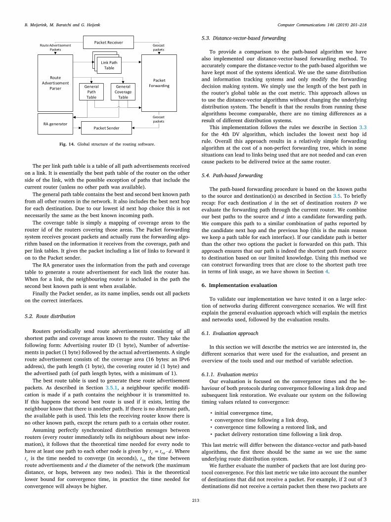
Our software consists of 8 main components, which are sharedby both implementations: The Packet receiver, Advertisement parser,Packet forwarding, Link path table, General path table, Coverage table,Route advertisement generator, and Packet sender. These componentsand their mutual relationships can be seen in Fig. 14. The generalstructure of the software is mostly identical for both algorithms, onlythe ‘‘Packet Forwarding’’ section has algorithm specific behaviour.

The packet receiver handles all incoming packets. Packets that havea geocast destination address are passed to the packet forwardingsystem while advertisement packets are passed to the advertisementparser.

The route advertisement parser parses the advertisement packet intopath data and coverage data. Path data consists of a path for each routerincluded in the advertisement. This data is given to the per link pathtable and the general path table. Coverage information consists of ageographic address of the coverage area and the id of the coveringrouter. This information is passed to the coverage table.

212


Fig. 14. Global structure of the routing software.

The per link path table is a table of all path advertisements receivedon a link. It is essentially the best path table of the router on the otherside of the link, with the possible exception of paths that include thecurrent router (unless no other path was available).

The general path table contains the best and second best known pathfrom all other routers in the network. It also includes the best next hopfor each destination. Due to our lowest id next hop choice this is notnecessarily the same as the best known incoming path.

The coverage table is simply a mapping of coverage areas to therouter id of the routers covering those areas. The Packet forwardingsystem receives geocast packets and actually runs the forwarding algo-rithm based on the information it receives from the coverage, path andper link tables. It gives the packet including a list of links to forward iton to the Packet sender.

The RA generator uses the information from the path and coveragetable to generate a route advertisement for each link the router has.When for a link, the neighbouring router is included in the path thesecond best known path is sent when available.

Finally the Packet sender, as its name implies, sends out all packetson the correct interfaces.

5.2. Route distribution

Routers periodically send route advertisements consisting of allshortest paths and coverage areas known to the router. They take thefollowing form: Advertising router ID (1 byte), Number of advertise-ments in packet (1 byte) followed by the actual advertisements. A singleroute advertisement consists of: the coverage area (16 bytes: an IPv6address), the path length (1 byte), the covering router id (1 byte) andthe advertised path (of path length bytes, with a minimum of 1).

The best route table is used to generate these route advertisementpackets. As described in Section 3.5.1, a neighbour specific modifi-cation is made if a path contains the neighbour it is transmitted to.If this happens the second best route is used if it exists, letting theneighbour know that there is another path. If there is no alternate path,the available path is used. This lets the receiving router know there isno other known path, except the return path to a certain other router.

Assuming perfectly synchronized distribution messages betweenrouters (every router immediately tells its neighbours about new infor-mation), it follows that the theoretical time needed for every node tohave at least one path to each other node is given by 𝑡𝑐 = 𝑡𝑟𝑎 ⋅𝑑. Where𝑡𝑐 is the time needed to converge (in seconds), 𝑡𝑟𝑎 the time betweenroute advertisements and 𝑑 the diameter of the network (the maximumdistance, or hops, between any two nodes). This is the theoreticallower bound for convergence time, in practice the time needed forconvergence will always be higher.

5.3. Distance-vector-based forwarding

To provide a comparison to the path-based algorithm we havealso implemented our distance-vector-based forwarding method. Toaccurately compare the distance-vector to the path-based algorithm wehave kept most of the systems identical. We use the same distributionand information tracking systems and only modify the forwardingdecision making system. We simply use the length of the best path inthe router’s global table as the cost metric. This approach allows usto use the distance-vector algorithms without changing the underlyingdistribution system. The benefit is that the results from running thesealgorithms become comparable, there are no timing differences as aresult of different distribution systems.

This implementation follows the rules we describe in Section 3.3for the 4th DV algorithm, which includes the lowest next hop idrule. Overall this approach results in a relatively simple forwardingalgorithm at the cost of a non-perfect forwarding tree, which in somesituations can lead to links being used that are not needed and can evencause packets to be delivered twice at the same router.

5.4. Path-based forwarding

The path-based forwarding procedure is based on the known pathsto the source and destination(s) as described in Section 3.5. To brieflyrecap: For each destination 𝑑 in the set of destination routers 𝐷 weevaluate the forwarding path through the current router. We combineour best paths to the source and 𝑑 into a candidate forwarding path.We compare this path to a similar combination of paths reported bythe candidate next hop and the previous hop (this is the main reasonwe keep a path table for each interface). If our candidate path is betterthan the other two options the packet is forwarded on this path. Thisapproach ensures that our path is indeed the shortest path from sourceto destination based on our limited knowledge. Using this method wecan construct forwarding trees that are close to the shortest path treein terms of link usage, as we have shown in Section 4.

6. Implementation evaluation

To validate our implementation we have tested it on a large selec-tion of networks during different convergence scenarios. We will firstexplain the general evaluation approach which will explain the metricsand networks used, followed by the evaluation results.

6.1. Evaluation approach

In this section we will describe the metrics we are interested in, thedifferent scenarios that were used for the evaluation, and present anoverview of the tools used and our method of variable selection.

6.1.1. Evaluation metricsOur evaluation is focused on the convergence times and the be-

haviour of both protocols during convergence following a link drop andsubsequent link restoration. We evaluate our system on the followingtiming values related to convergence:

• initial convergence time,• convergence time following a link drop,• convergence time following a restored link, and• packet delivery restoration time following a link drop.

This last metric will differ between the distance-vector and path-basedalgorithms, the first three should be the same as we use the sameunderlying route distribution system.

We further evaluate the number of packets that are lost during pro-tocol convergence. For this last metric we take into account the numberof destinations that did not receive a packet. For example, if 2 out of 3destinations did not receive a certain packet then these two packets are

213


Fig. 15. Examples of convergence behaviour on different networks. (For interpretation of the references to colour in this figure legend, the reader is referred to the web versionof this article.)

considered lost. Using this method we hope to accurately represent thenumber of deliveries that were missed during the convergence time.

We will also look at the possible multi-path issues during a con-vergence phase, in which packets are delivered to a router over mul-tiple paths. Ideally this should never occur, but it is likely unavoid-able during protocol convergence due to incomplete or outdated net-work knowledge in different routers. In the case of the distance-vectorbased protocol, we expect larger numbers of duplicate packets as theinformation to build a perfect shortest path tree is just not available.

As a base-line for how efficient the protocols construct their for-warding path we will look at the link usage. We use a normalizedlink usage metric to more easily compare efficiency between differentnetworks. This normalization is done by describing the link usage as afraction of the total number of links in a network.

6.1.2. Evaluation scenarioWe start each evaluation run by giving the routing algorithm time

to converge. We have set this waiting time to 25 s as we have notobserved the convergence taking longer than this time. After this initialtime, we start transmitting packets from a randomly selected source to arandomly selected destination area. 10 s after the transmissions start wedrop a randomly chosen link on the forwarding tree for those packets.We measure how long it takes the algorithm to converge again and theeffect this has on the packets that are in transit during this time. 50 safter the link drop, we restore the link and we measure the convergenceduration again. We also measure the number of packets lost during theentire run.

6.1.3. Networks and variable selectionLike the evaluation in Section 4, we use real world network graphs

taken from the Topologyzoo project [21] to evaluate our protocol on aset of realistic networks. We used a total of 162 networks, those rangingin size from 6 to 51 routers, with an average of 26 routers. In the case anetwork is not connected, we use the largest connected part. We importthese networks into a Mininet virtual network [24] by generating anew node running our routing implementations for each vertex in thegraph and establishing a link (1 Gb/s Ethernet) between nodes if thecorresponding graph has an edge.

The latitude and longitude location (as given in the Topologyzoo)of the node is used to generate a coverage area of a size correspondingto depth 10 of our addressing scheme (Section 2.2) to ensure routerscover reasonable portions of a network. For each run within a networka destination area is randomly generated. This area can cover between10% and 95% of the bounding box containing all nodes in the network.We also randomly select a source router for each run, this router canbe inside or outside the destination area.

To emulate a link drop we set both ends of a link to have a 100%packet loss rate using the Linux network emulator [25] functionality.The link to drop is chosen randomly from the set of links on the shortestpath tree from the source to the destinations. With this link selectionwe try to guarantee that the dropped link will at least have some effecton the forwarding situation. The dropped link is chosen in such a waythat is does not lead to a disconnected network, so the algorithm canactually converge to the new situation and still reach all destinations.

Routers are configured to exchange route advertisements every0.5 s. Route entries expire after two seconds, leading to a relativelyfast update time.

The distance-vector and path-based algorithm are run on the sameset of networks with the same sources and destinations. The link thatis dropped from the network is also kept identical between the twodifferent algorithms. Due to the way a dropped link is chosen andthe way our algorithms construct their forwarding trees, it is notguaranteed this link is on the forwarding tree all the time. For bothalgorithms the dropped link was on the forwarding tree 92% of the runs.

6.2. Results

In this section we will present our results. We start with an overviewof our algorithm’s performance in a converged state and continue withthe convergence time of the protocol in different network states. Weend the section with an analysis of packet loss and duplicate packetdelivery during different convergence situations.

6.2.1. Example runsTo better explain our experimental results, we show the conver-

gence behaviour of runs in two different networks in Fig. 15. On the left𝑦-axis (blue line) we show the normalized distribution tree cost where100% corresponds to the link usage of the initial distribution tree. Onthe right 𝑦-axis (yellow line) we show packet loss as the number ofdestination routers that did not receive a packet at a certain time. The𝑥-axis shows the elapsed time from the start of the packet transmissionsin seconds. The time of the link drop is marked as a dotted red verticalline and the link restore time with a dotted green vertical line. Thedotted blue vertical lines mark the time at which the protocol hasconverged to the new situation.

We can see that immediately following the loss of a link there is aperiod of packet loss, but packet delivery is restored before the networkhas fully converged. This can be explained by the fact that the linkloss (almost always) occurs on a path that is used, resulting in localconvergence before the protocol in the entire network has had time toconverge. A similar pattern can be seen following the link restore, butthe packet loss is minimal here. This is likely caused by the fact that

214


Fig. 16. Normalized link usage in a converged network.

information about new link propagates faster compared to informationof lost links due to the way that time-outs function. The small red linesthat can be seen following the link restoration represent packets thatarrived multiple times at a router in the network. Packets are sometimesrouted over multiple paths during convergence, temporarily increasinglink usage as can be seen in the graphs. The normalized distribution treecosts decreases after the link loss as the forwarding tree does not reachthe destination nodes any more. Eventually the protocol convergesand the normalized cost exceeds 100%, due to the larger tree that isneeded to route around the missing link. Following the restoration ofthe dropped link we can see the normalized cost return to 100% as theprotocol returns to using the initial distribution tree.

6.2.2. General link usageIn Fig. 16 we plot the link usage of both our implementations

against the shortest path tree and a Steiner tree for the same (source,destination) tuples. The shortest path and Steiner tree link usage are asubset of the data used for Fig. 12 limited to the (source, destination)tuples used here. On the 𝑦-axis we show the average of the normalizedvalue of the link usage, meaning the number of links used to reachall destinations divided by the number of links in the network. The𝑥-axis shows the number of destinations addressed and below that,the number of runs with this number of destinations in brackets.The difference in number of runs is a consequence of our destinationarea generation system, which chooses areas with a small number ofrouters in geographically large networks. The error bars show the 95%confidence interval for that value. Runs with more than 10 destinationwere not numerous enough to provide statistically significant results.

In general our path-based protocol establishes forwarding trees thatuse a comparable number of links compared to a shortest path tree.In our 2916 runs there were only 392 runs (13%) where the path-based algorithm established a path with a different number of linksthan the shortest path tree. In most of these cases (238) this pathwas one link longer, and in some rare cases (154) one shorter. Theformer can in some cases be explained by minor inefficiencies, and thelatter difference can be explained by situations where there are multipleshortest paths from the source to a single destination. If the chosen pathoverlaps with that of another destination the resulting link usage canbe lower compared to the situation where the other path was taken.

The distance-vector algorithm has a higher link usage compared tothe path-based one. The main cause of this is that multiple links aresometimes used to reach the same destination. The higher transmissioncost is offset by a simpler algorithm. For this algorithm, 1130 runs(39%) had a different link usage compared to the shortest path tree.A total of 1037 runs had a higher link cost while 93 runs had alower cost. As with the path-based algorithm, the lower link costs were

caused by situations were multiple shortest paths were available, andsome overlapped. This result corresponds with the initial results fromSection 4.

We can conclude that our path-based protocol performs mostlyas expected with respect to the number of links used to construct aforwarding tree. Our distance-vector based protocol has significantlyhigher link usage.

6.2.3. Convergence timeOne of the more important aspects of any routing protocol is the

time it takes to converge following a change in the network. Thecorrelation between the network size (the number of routers in thenetwork) and the time convergence takes during the evaluation isshown in Fig. 17 for path-based and DV-based routing. In these figureswe show per network averages as points, the lines represent the averageover all runs. We can see that the initial convergence time (blue line) ofthe network shows a strong correlation to the network size. As a largernetwork mostly corresponds to more possible paths it correlates withthe time it takes for the algorithm to converge.

Both the path-based and distance-vector graphs show comparableresults for the convergence times. This is the result of both usingthe same underlying route distribution method. Small differences arecaused by differences in the exact time nodes started in relation to eachother combined with the time-out of 2 s.

On average the convergence time after a link drop (red line) issignificantly larger than that of adding or restoring a link (green line)to the network. As noted before this can be explained by the time-outof 2 s that needs to occur before link loss is propagated while new linksare advertised with at most a 0.5 s delay.

One of the interesting things to note in this graph, is that the timeto convergence after a link restoration (green line) is lower than theinitial convergence time (blue line) for larger networks. We expect thisis caused by the locality of the change. In larger networks a single linkchange is not likely to affect path entries further away in the network,although this does strongly depend on how well connected the networkis.

For the path-based protocol, the time it takes for full packet deliveryto be restored after a link drop (orange striped line) follows a similarpattern as the link drop convergence time, but takes less time overall(Fig. 17a). The distance-vector protocol shows behaviour more like thelink restore convergence time (Fig. 17b). The main difference betweenthe packet delivery restoration time in both protocols is that the path-based method seems to perform worse in networks with 15 to 35nodes, but better in larger networks. This effect is likely caused bythe location of the dropped link in relation to the destination nodes.In relatively small networks it is more likely that a destination is closeto a dropped link leading to a lower chance that the path-based methodhas an obvious route around the problem. The distance-vector approachhas no knowledge of these paths and simply attempts (an inefficient)alternative path once it knows about the missing link.

6.2.4. Behaviour during convergenceAs can be expected, during the convergence directly following a link

drop, a number of packets is not delivered to the destination routers.We plot these losses for the path-based algorithm in Fig. 18a and forthe distance-vector based results in Fig. 18b. In these figures, the reddots represent the number of routers that did not receive a packet ina certain simulation run at that time. The intensity of the red colourcorresponds to the number of runs in which this number of packetswas lost at that particular time. Barely visible dots represent a singleoccurrence. The blue line represents the percentage of runs in whichpacket loss occurred at that time. Note that while we plot the red andgreen dotted line to represent the link drop and restoration point, thisdoes not correspond to the exact drop time in all simulation runs. Thiscan be seen by dropped packets that occur earlier than expected. Thereare two causes for this effect: the varying start-up time in the emulation,

215


Fig. 17. Convergence times of all runs in the evaluation. (For interpretation of the references to colour in this figure legend, the reader is referred to the web version of thisarticle.)

Fig. 18. Packet loss data.

mostly depending on network size, and the fact that packets losses areplotted based on the time their packet entered the network. We believethis is the best approach to keep networks of different sizes comparableas this would otherwise have an effect on the time they are lost.

Packet loss mainly occurs after a link drop, and link restorationbarely leads to any lost packets. The distance-vector-based routing algo-rithm actually seems to restore packet delivery slightly faster comparedto the path-based algorithm. The packet loss during link restorationfor the distance-vector protocol is twice as high compared to thepath-based protocol.

While our routing system should not route packets in a loop it doesin some specific conditions route packets to a single router throughmultiple paths. This effect can occur during convergence when thenetwork is temporarily in a configuration that allows a multi pathsituation to occur. This effect can be observed in Figs. 15a and 15bas a solid red line. We can see this line corresponds to the small peakin path cost directly following the restoration of a link. We show theoverall duplicate packet delivery rate for both algorithms in Fig. 19. Inthese figures the red dots represent the number of routers in a certainrun that received a certain packet twice, or more times. As with theloss graphs, the 𝑥-axis represents the time at which the packet wassent from the source router measured from the start of a run. The blueline represents the percentage of runs in which a packet was receivedmultiple times by any router. As we can see this effect mainly occurswhen a link is restored (or added) to the network. While the path-basedapproach only has some duplicate deliveries during link restoration, the

distance-vector approach appears to have duplicate deliveries all thetime. These consistent duplicate packets are caused by the algorithmdelivering packets over multiple routes to a single destination in somecases, as explained in Sections 3.3 and 3.4.

Compared to unicast routing we avoid certain issues in our path-based approach, like the count to infinity problem, by relying only onpath information. Packets are simply not forwarded any more if a routerfinds itself on anything but the shortest path from its point of view. Onthe topic of network change we can conclude that our protocol correctlyre-establishes a forwarding tree with only temporary problems, such asa router receiving packets over multiple links, in some cases followinga link restoration.

7. Conclusions and future work

In this paper, we have presented a purely distance-vector and apath-based algorithm for geographic routing. We have also presentedimplementations of both protocols. For the path-based approach, wehave shown that the protocol forwards packets along a tree close tothe shortest path tree in terms of links used when the network isstable. The Distance-Vector protocol performs worse compared to thepath-based one, but is less complex in terms of forwarding rules andrequired information. We have also shown that during periods wherethe network changes our protocols can recover in a reasonable time.The time it takes our protocols to recover depends on factors likenetwork size and how well connected the network is.

216


Fig. 19. Duplicate packet delivery data.

We have shown that our best distance-vector-based algorithm per-forms relatively well, and in the worst case has only 32% more linkcost compared to the shortest path tree. In a situation where the entirenetwork is not addressed this overhead is even lower. Our path-basedalgorithm can construct forwarding trees to multiple destinations thatare close in link cost to the shortest path tree from the source toall destinations. This algorithm improves on the distance-vector-basedalgorithm, especially in situations where a large number of routers inthe network (> 25%) are part of the addressed area.

During network convergence due to link failure we lose packets inboth algorithms as can be expected. The algorithms do however recoverfrom this state in a reasonable time. Following a link restoration thereis only minimal packet loss in both cases. The path-based protocol doesdeliver packets over multiple routes to a destination in this situation.While this effect is not desirable it seems limited to certain networktopologies and does to some degree prevent packet loss from occurring.The distance-vector approach suffers from duplicate deliveries in moresituations.

We believe that the distance-vector algorithm might actually bepreferable in certain situations where the extra computational overheadin the router does not outweigh the extra transmission overhead inthe network. We expect that this routing approach combined with ahierarchical approach in which autonomous systems advertise one ormore areas will eventually allow Internet-wide geocast to become areality.

To achieve functioning geocast, further work will need to be done.Areas of special interest are hierarchical routing, security and last hopdistribution methods.

Hierarchical routing is needed so different autonomous systemscan distribute coverage and reachability information. Further work isneeded to research methods to extend our current routing proposal tothis level.

The are several security issues mostly relating to the possibilityof denial of service attacks in the current proposal that need to beaddressed. Further work is needed on limiting geocast capabilities tocertain users, or limiting the area addressed to prevent wide scaledenial of service attacks using geocast.

Work needs to be done on the final hop towards mobile devices, in-cluding vehicles. The hop towards end-user devices presents a challengefor geographically scoped communication. There are several differentsituations in which the method of distribution would need to be tailoredto the specific situation. While our addressing method can address smallareas, addressing a specific road for example, would still require someform of translation to limit the message to just that road, and not thesurrounding area.

For future work, we are planning to improve our information dis-tribution method. In the current implementation coverage area and

the path to the covering router are tightly linked. We would like tocompletely decouple these things to increase scalability. Coverage areainformation does not need to be advertised as often as path information,and this change could thus decrease overhead. In general our routingprotocols, especially with these improvements, can provide anotherstep in enabling Internet-wide geocast in the future.

Declaration of competing interest

The authors declare that they have no known competing finan-cial interests or personal relationships that could have appeared toinfluence the work reported in this paper.

References

[1] G. Karagiannis, G. Heijenk, A. Festag, A. Petrescu, A. Chaiken, Internet-wide geo-networking problem statement, URL https://tools.ietf.org/html/draft-karagiannis-problem-statement-geonetworking-01.

[2] J.C. Navas, T. Imielinski, GeoCast - geographic addressing and routing, in: L. Pap,K. Sohraby, D.B. Johnson, C. Rose (Eds.), MOBICOM, ACM, 1997, pp. 66–76.

[3] F. Cunha, L. Villas, A. Boukerche, G. Maia, A. Viana, R.A. Mini, A.A. Loureiro,Data communication in vanets: Protocols, applications and challenges, Ad HocNetw. 44 (2016) 90–103.

[4] T. Fioreze, G.J. Heijenk, Extending the domain name system (DNS) to providegeographical addressing towards vehicular ad-hoc networks (VANETs), in: O.Altintas, W. Chen, G.J. Heijenk (Eds.), VNC, IEEE, 2011, pp. 70–77.

[5] J.C. Navas, T. Imielinski, On reducing the computational cost of GeographicRouting, Rutgers University, Department of Computer Science, Tech. Rep.DCS-TR-408.

[6] T. Imielinski, S. Goel, Dataspace - querying and monitoring deeply networkedcollections in physical space, in: MobiDE, ACM, 1999, pp. 44–51.

[7] M. Di Felice, L. Bedogni, L. Bononi, Group communication on highways: Anevaluation study of geocast protocols and applications, Ad Hoc Netw. 11 (3)(2013) 818–832.

[8] B.T. Sharef, R.A. Alsaqour, M. Ismail, Vehicular communication ad hoc routingprotocols: A survey, J. Netw. Comput. Appl. 40 (2014) 363–396.

[9] J. Liu, J. Wan, Q. Wang, P. Deng, K. Zhou, Y. Qiao, A survey on position-basedrouting for vehicular ad hoc networks, Telecommun. Syst. 62 (1) (2016) 15–30.

[10] Y.-B. Ko, N.H. Vaidya, Geotora: A protocol for geocasting in mobile ad hoc net-works, in: Network Protocols, 2000. Proceedings. 2000 International Conferenceon, IEEE, 2000, pp. 240–250.

[11] B. Karp, H.-T. Kung, Gpsr: Greedy perimeter stateless routing for wirelessnetworks, in: Proceedings of the 6th Annual International Conference on MobileComputing and Networking, ACM, 2000, pp. 243–254.

[12] J. Li, J. Jannotti, D.S. De Couto, D.R. Karger, R. Morris, A scalable locationservice for geographic ad hoc routing, in: Proceedings of the 6th AnnualInternational Conference on Mobile Computing and Networking, ACM, 2000,pp. 120–130.

[13] D. Farinacci, T. Li, S. Hanks, D. Meyer, P. Traina, Protocol independentmulticast-dense mode (pim-dm): Protocol specification (revised), RFC 3973.

[14] B. Fenner, M. Handley, I. Kouvelas, H. Holbrook, Protocol independentmulticast-sparse mode (PIM-SM): protocol specification (revised).

217

https://tools.ietf.org/html/draft-karagiannis-problem-statement-geonetworking-01



http://refhub.elsevier.com/S0140-3664(18)30986-1/sb2













































[15] D. Moscoviter, M. Gholibeigi, B. Meijerink, R. Kooijman, P. Krijger, G. Heijenk,Improving spatial indexing and searching for location-based dns queries, in:International Conference on Wired/Wireless Internet Communication, Springer,2016, pp. 187–198.

[16] B. Meijerink, M. Baratchi, G. Heijenk, An efficient geographical addressingscheme for the internet, in: International Conference on Wired/Wireless InternetCommunication, Springer, 2016, pp. 78–90.

[17] L. Kou, G. Markowsky, L. Berman, A fast algorithm for steiner trees, Acta Inform.15 (2) (1981) 141–145.

[18] M. Doar, I. Leslie, How bad is naive multicast routing? in: INFOCOM’93.Proceedings. Twelfth Annual Joint Conference of the IEEE Computer andCommunications Societies. Networking: Foundation for the Future, IEEE, IEEE,1993, pp. 82–89.

[19] U.T. Nguyen, J. Xu, Multicast routing in wireless mesh networks: Minimum costtrees or shortest path trees? IEEE Commun. Mag. 45 (11) (2007) 72–77.

[20] B. Meijerink, M. Baratchi, G. Heijenk, Evaluation of geocast routing trees onrandom and actual networks, in: International Conference on Wired/WirelessInternet Communication, Springer, 2017, pp. 127–142.

[21] S. Knight, H. Nguyen, N. Falkner, R. Bowden, M. Roughan, The internet topologyzoo, IEEE J. Sel. Areas Commun. 29 (9) (2011) 1765–1775, http://dx.doi.org/10.1109/JSAC.2011.111002.

[22] Y. Rekhter, T. Li, S. Hares, A border gateway protocol 4 (BGP-4), Tech. rep.,2005.

[23] A.A. Hagberg, D.A. Schult, P.J. Swart, Exploring network structure, dynamics,and function using NetworkX, in: Proceedings of the 7th Python in ScienceConference (SciPy2008), Pasadena, CA USA, 2008, pp. 11–15.

[24] Mininet Project, Mininet. URL http://mininet.org.[25] Linux Foundation, netem. URL http://www.linuxfoundation.org/collaborate/

workgroups/networking/netem, 2009.

218































http://dx.doi.org/10.1109/JSAC.2011.111002








http://mininet.org

http://www.linuxfoundation.org/collaborate/workgroups/networking/netem



design & analysis of a distributed routing algorithm

Documents