Description of massive neutrinos. The origin of the neutrino mass

Steve King, Erice, 18th September, 2013

Description of Massive Neutrinos

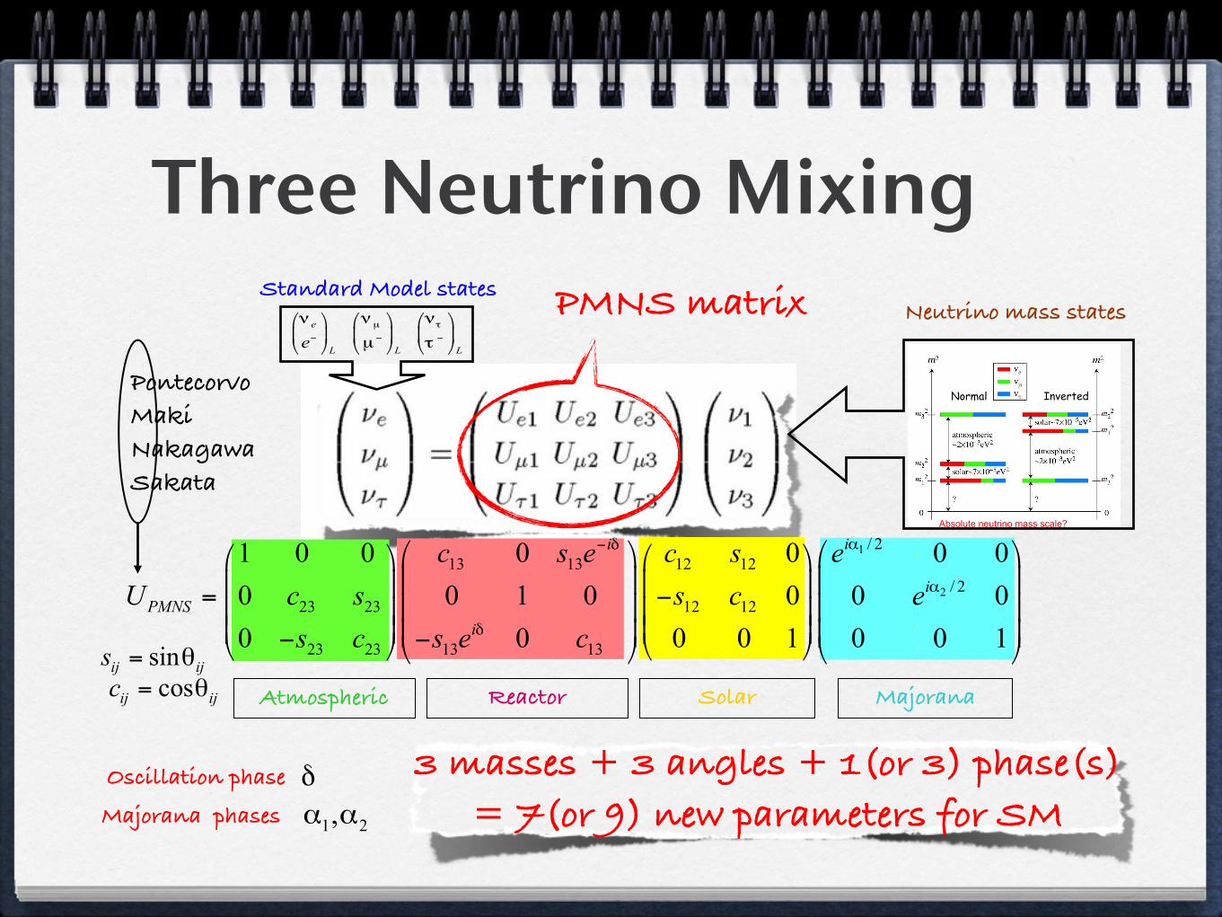
Three Neutrino MixingStandard Model states

Neutrino mass states

Oscillation phase 3 masses + 3 angles + 1(or 3) phase(s) = 7(or 9) new parameters for SM

Atmospheric Reactor Solar

c

.d=

.

.

.

.

.

.

Majorana

Majorana phases

PontecorvoMakiNakagawaSakata

.

.

.

Normal Inverted

Absolute neutrino mass scale?

PMNS matrix

Forero et al

Fogli et al

Gonzalez!Garcia et alNO

0.25 0.30 0.35 0.40

sin2"12

Forero et al

Fogli et al

Gonzalez!Garcia et alNO

0.3 0.4 0.5 0.6 0.7

sin2"23

Forero et al

Fogli et al

Gonzalez!Garcia et alNO

0.00 0.01 0.02 0.03 0.04

sin2"13

Forero et al

Fogli et al

Gonzalez!Garcia et alIO

0.25 0.30 0.35 0.40

sin2"12

Forero et al

Fogli et al

Gonzalez!Garcia et alIO

0.3 0.4 0.5 0.6 0.7

sin2"23

Forero et al

Fogli et al

Gonzalez!Garcia et alIO

0.00 0.01 0.02 0.03 0.04

sin2"13

Figure 4: The mixing angles obtained from the three global fits [56–58]. The upper three panelscorrespond to the results for normal neutrino mass ordering (NO), while the lower three panels arefor an inverted mass ordering (IO). Shown are the best fit values (green) as well as the 1! (red)and 3! (blue) intervals. Note that the solar angle is insensitive to the mass ordering.

Gonzalez-Garcia et al [58]. The results for the mixing angles are graphically contrasted in

Fig. 4. We emphasise that this compilation is predominantly meant to illustrate some pos-

sibilities arising from present global fits. The reader is referred to the respective references

for the subtleties associated with these numbers.

For the normal mass ordering, we shall take the average values and errors which ap-

proximately encompass the one sigma ranges of all three global fits (ignoring the solution

of "23 in the second octant found by Forero et al [56]):

sin2 "12 = 0.31 ± 0.02, (2.20)

sin2 "23 = 0.41 ± 0.05, (2.21)

sin2 "13 = 0.024 ± 0.003. (2.22)

These values may be compared to the tri-bimaximal predictions sin2 "12 = 0.33, sin2 "23 =

0.5 and sin2 "13 = 0, showing that TB mixing is excluded by the reactor angle. Alternatively

we may write, remembering that these are one sigma ranges in the squares of the sines and

not the sines themselves,

sin "12 = 0.56 ± 0.02, (2.23)

sin "23 = 0.64 ± 0.04, (2.24)

sin "13 = 0.155 ± 0.01. (2.25)

– 20 –

Global Fits 2012 SFK and C.Luhn, ``Neutrino Mass and Mixing with Discrete Symmetry,'' arXiv:1301.1340

35◦ 45◦ 0◦

Neutrino Mixing QuestionsIs the atmospheric angle maximal 450?

If not then which octant?

Is the solar angle trimaximal 35o?

If not then less or greater?

Is the CP phase special 0, pi, pi/2, ...?

If not then what is it?

Origin of neutrino mixing?

What is the mass squared ordering (normal or inverted) ?

What is the neutrino mass scale (mass of lightest neutrino)?

What is the nature of neutrino mass (i.e. Dirac or Majorana)?

Origin of neutrino mass?

Neutrino Mass Questions Normal Inverted

Absolute neutrino mass scale?

b

cs

ud

e

t

The Flavour ProblemWhat is the origin of quark and lepton masses?

Why are neutrino masses so small?

The Electron Mass

Dirac

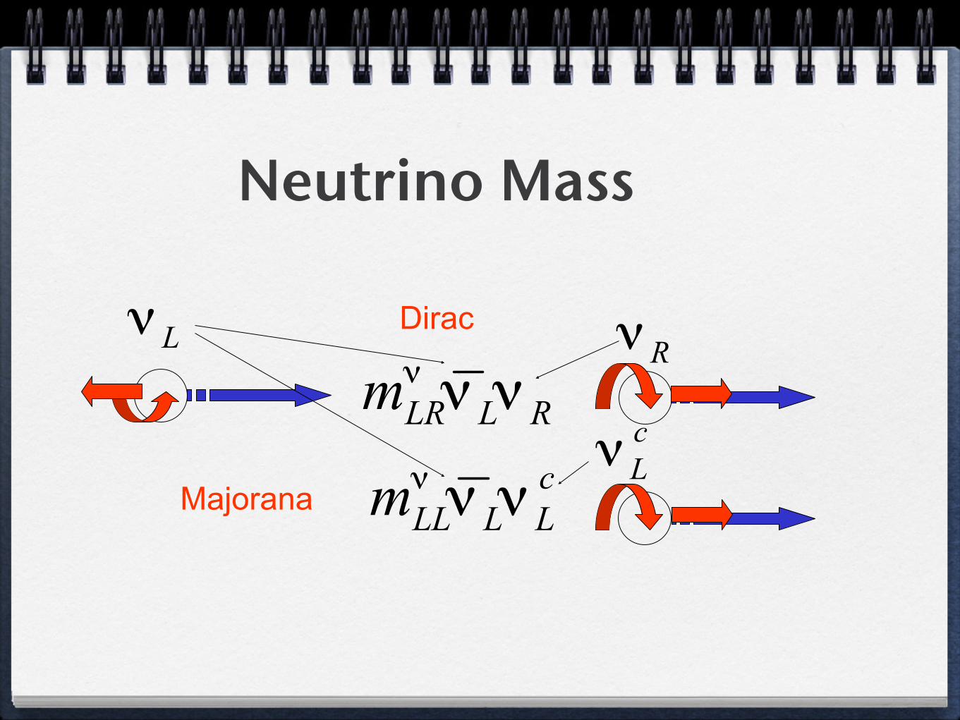
Dirac

Majorana

Neutrino Mass

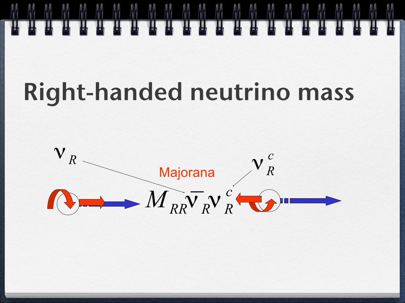
Right-handed neutrino mass

Majorana

Majorana masses

Conserves L Violates

CP conjugate

Dirac mass

Violates L Violates

Summary of Neutrino Masses

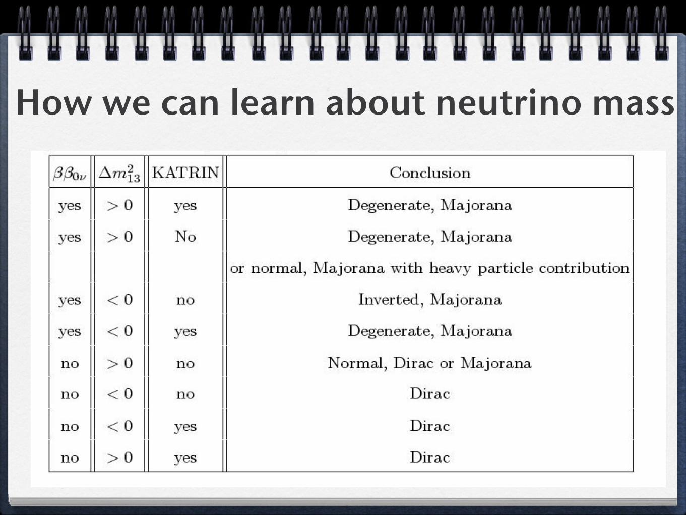
How we can learn about neutrino mass

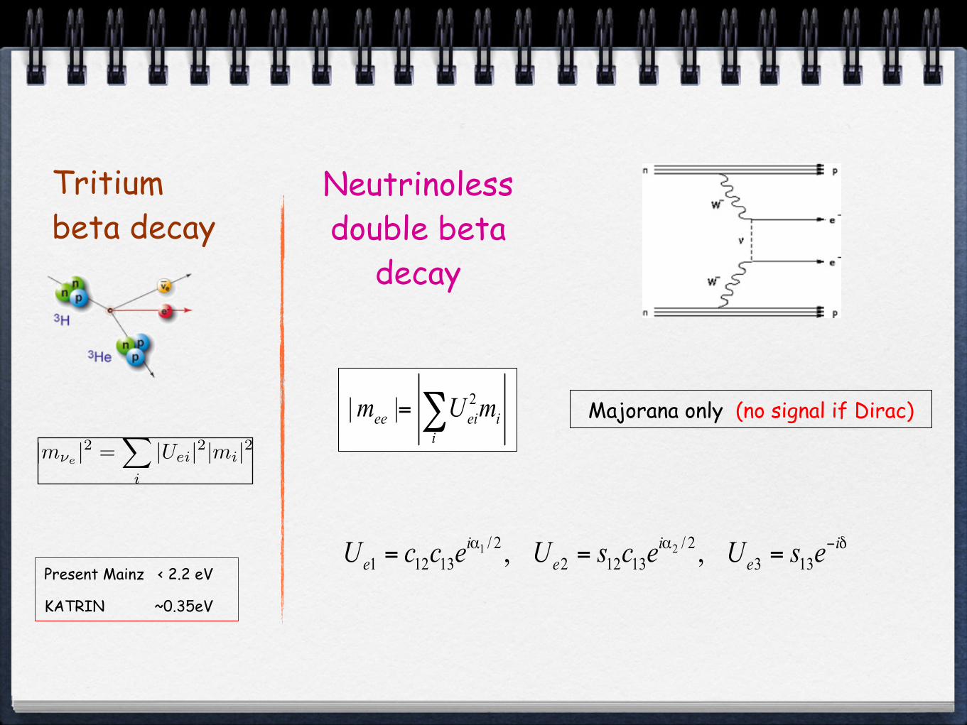
Neutrinoless double beta

decay

Tritium beta decay

Present Mainz < 2.2 eV

KATRIN ~0.35eV

Majorana only (no signal if Dirac)

|mνe |2 =�

i

|Uei|2|mi|2

Current and Future LimitsIsotope Current Limits T 0νββ

1/2 [y] |mee| [eV] |mee| outliers Refs.76Ge HD-Moscow > 1.9 · 1025 0.26(M5)–0.32(M1) 0.65(M2) [133]

IGEX > 1.57 · 1025 0.28(M5)–0.36(M1) 0.71(M2) [134]GERDA I > 2.1 · 1025 0.24(M5)–0.31(M1) 0.61(M2) [23]

82Se NEMO-3 > 3.2 · 1023 0.97(M5)–1.3(M1) 2.5(M2) [135]100Mo NEMO-3 > 1.1 · 1024 0.41(M7)–0.49(M6) 0.70(M3) [135]130Te Cuoricino > 2.8 · 1024 0.29(M1)–0.40(M8) 0.71(M2),1.1(M9) [136]136Xe KamLAND-Zen > 1.9 · 1025 0.13(M1)–0.34(M9) —– [132]

EXO-200 > 1.6 · 1025 0.15(M1)–0.37(M9) —– [46]

Isotope Future Limits T 0νββ1/2 [y] |mee| [eV] |mee| outliers Refs.

76Ge GERDA II > 2 · 1026 0.079(M5)–0.10(M1) 0.20(M2) [24,25]GERDA III > 6 · 1027 0.014(M5)–0.018(M1) 0.036(M2) [24,25]Majorana > 2 · 1026 0.079(M5)–0.10(M1) 0.20(M2) [137,138]

82Se SuperNEMO > 2 · 1026 0.039(M5)–0.052(M1) 0.10(M2) [139,140]130Te CUORE > 6.5 · 1026 0.019(M1)–0.026(M8) 0.047(M2),0.072(M9) [141,142]136Xe KamLAND-Zen > 1 · 1027 0.019(M1)–0.046(M9) —– [131]

EXO-1000 > 8 · 1026 0.021(M1)–0.052(M9) —– [143,144]150Nd SNO+ > 3 · 1025 0.068(M9)–0.12(M1) —– [131]

Table 3: The derived ranges for |mee| for several current experimental limits and futureexperimental sensitivities [131]. For each isotope, we report the name the respectiveexperiments and the 90% C.L.-limits for the half-life T 0νββ

1/2 . For the effective mass wealways indicate the minimal and maximal values (depending on the NME). In case someNMEs result into values for |mee| which differ considerably from the ones obtained by theother methods, we list these results separately as “outliers”.

to have a comparison of several measurements of 0νββ on different isotopes in order tofully disentangle the nuclear physics complications, and also to decide which isotopes tochoose for future experiments.

9 Predictions of the different sum rules

In the following tables, we will list the predictions for the range of |mee| as well as anapproximate15 range for the smallest mass mlightest as obtained from the sum rules fromSec. 7.15. Note that, whenever a certain sum rule does not lead to a restricted rangecompared to the standard case displayed in Fig. 2, we will indicate this by “usual” (e.g.,if the minimum of |mee| is smaller than 0.0001 eV). When a certain ordering is not at all

15Our numerical procedure renders the estimate of mlightest a little less accurate than that of |mee|.

48

SFK, Merle, Stuart

Neutrino Mass Sum Rules

m1 +m2 = m3

1

m1+

1

m2=

1

m3

Rule 1

Rule 2

SFK, Merle, Stuart

GERDA I

10�4 0.001 0.01 0.1 110�4

0.001

0.01

0.1

1

mlightest �eV�

�m ee��eV�

DisfavouredbyCosmology

Disfavoured by 0ΝΒΒ

�m312 � 0

�m312 � 0

Best& 3Σ

Rule 1

Rule 2

GERDA II

GERDA III

Figure 1: The power of sum rules. Two example sum rules (rule 1: m̃−11 + m̃−1

2 = m̃−13

indicated by the forked red region, rule 2: m̃1 + m̃2 = m̃3 indicated by the violet region)are displayed, along with the result of GERDA phase I [23] and the maximum sensitivitiesof GERDA [24,25] for phase II and phase III, including the nuclear physics uncertaintieswhich generate the gaps between the horizontal green lines. Even with these uncertainties,the inverted ordering region of rule 1 is clearly falsifiable, thereby illustrating the powerof the sum rules. Technical details will be given later in the text.

neutrinoless double beta decay was observed. Thus it is worth to carefully discuss thispoint and to correct some of the results obtained previously. Secondly, it is known thata relatively large value of θ13, such as the one measured, can considerably influence theallowed regions for |mee| [29], which is particularly true when additional constraints suchas mass sum rules are imposed, and which makes an updated study worthwhile. Thirdly,the studies performed up to now have focused on the phenomenology of |mee|, withouta complete discussion of the experimental prospects, in particular in what regards thenuclear physics uncertainties. We close all these gaps by not only providing a detailedstudy of all neutrino mass sum rules we were able to find in the literature, but we alsodiscuss the prospects of many current and future experiments on neutrinoless doublebeta decay, thereby taking into account nine different methods to calculate the so-callednuclear matrix elements. We also provide a complete classification of all flavour modelsknown to us which lead to neutrino mass sum rules, so that a fairly complete picture of

2

Give restricted regions

Sum Rule Group Seesaw Type Matrixm̃1 + m̃2 = m̃3 A4 [21, 54, 61–64]; S4 [66]; A5 [65]∗ Weinberg Mν

m̃1 + m̃2 = m̃3 ∆(54) [67]; S4 [20] Type II ML

m̃1 + 2m̃2 = m̃3 S4 [95] Type II ML

2m̃2 + m̃3 = m̃1 A4 [16, 21, 61–64,77,79–86] Weinberg Mν

S4 [88, 96]†; T � [78, 89–93]; T7 [94]2m̃2 + m̃3 = m̃1 A4 [87] Type II ML

m̃1 + m̃2 = 2m̃3 S4 [97]‡ Dirac‡ Mν

m̃1 + m̃2 = 2m̃3 Le − Lµ − Lτ [98] Type II ML

m̃1 +√3+12 m̃3 =

√3−12 m̃2 A�

5 [100] Weinberg Mν

m̃−11 + m̃−1

2 = m̃−13 A4 [21]; S4 [20, 54]; A5 [39, 55] Type I MR

m̃−11 + m̃−1

2 = m̃−13 S4 [20] Type III MΣ

2m̃−12 + m̃−1

3 = m̃−11 A4 [15, 16, 18, 21,68–77,101]; T � [78] Type I MR

m̃−11 + m̃−1

3 = 2m̃−12 A4 [58, 59, 102]; T � [60] Type I MR

m̃−13 ± 2im̃−1

2 = m̃−11 ∆(96) [38] Type I MR

m̃1/21 − m̃1/2

3 = 2m̃1/22 A4 [19] Type I MD

m̃1/21 + m̃1/2

3 = 2m̃1/22 A4 [99] Scotogenic hν

m̃−1/21 + m̃−1/2

2 = 2m̃−1/23 S4 [53] Inverse MRS

Table 2: A sample of the various sum rules found in the literature and the groups gener-ating them, where the sume rules which are grouped together give identical predictions.∗In this reference, the sum rule was only used as a consistency relation. † Note that inRef. [96] the Majorana phases were predicted to have trivial values, which is why theprediction of that concrete model is stronger than our general prediction from the sumrule only. ‡Even though this reference predicts a sum rule, it features Dirac neutrinos.

8 Experimental perspectives of and nuclear physics

impact on 0νββ

We now want to discuss the experimental status and prospects of 0νββ. The generalproblem is that a potential observation of 0νββ would only give us an experimentalmeasurement of the decay rate or the half-life, while what we actually would like to knowis the amplitude, and in particular the value of the quantity |mee|. If indeed light neutrinoexchange (as discussed above) dominates the decay rate, then the half-life T 0ν

1/2 can beobtained by the following equation [108],

1

T 0ν1/2

= G0ν |M0ν |2�|mee|me

�2

, (117)

44

Sum Rules in ModelsSFK, Merle, Stuart

Predictions of sum rules

10�4 0.001 0.01 0.1 1�mee� �eV�

m� 1 � m� 2 � m� 3m� 1 � m� 3 � 2m� 22m� 2 � m� 3 � m� 1m� 1 � m� 2 � 2 m� 3

m� 1 � 3 �12 m� 3 � 3 �1

2 m� 2m� 1�1 � m

�2�1 � m� 3�1

2m� 2�1 � m�3�1 � m� 1�1

m� 1�1 � m�3�1 � 2m� 2�1

m� 3�1 � 2im�2�1 � m� 1�1

m� 1 � m� 3 � 2 m� 2m� 1 � m� 3 � 2 m� 2m� 1�1�2 � m� 2�1�2 � 2m� 3�1�2Disfavouredby0ΝΒΒ

GMSS

Figure 20: Graphical representation of the predictions of the different sum rules.

possible for the sum rule under consideration, we instead use the term “forbidden”. Note

that we have decided to report only the 3σ predictions, since the best-fit values show a

considerable variation depending on which gobal fit is used. This is a reflection of the fact

that the region where the effective mass tends to zero arises due to a delicate cancellations

between the different contributions [29], so that slightly altered best-fit values could lead

to quite different results (as can be seen by comparing the best-fit regions obtained with

the three different fits in, e.g., Secs. 7.4 and 7.13). The 3σ results, on the other hand, are

much more stable and reliable predictions. We have obtained the predictions (which are

always given in eV) displayed in Tabs. 4, 5, and 6.

Finally, we have graphically represented the predictions of all sum rule for the effectivemass |mee| in Fig. 20. Together with the information on the experimental sensitivities and

on the ranges of the NME calculations given in Sec. 8, these predictions allow to determine

whether a certain sum rule can be fully or partially probed by a certain experiment, even

if nuclear physics uncertainties blur the picture. We have illustrated in Fig. 1 that this

is indeed possible in some cases. However, different scientific opinions exist about one or

the other experiment, about one or the other global fit, or about one or the other method

to calculate nuclear matrix elements. Thus we leave it to the reader to decide which rules

they consider to be falsifiable with a given experiment. We have with this paper delivered

50

SFK, Merle, Stuart

The Origin of Neutrino Mass

1. There are no right-handed neutrinos

2. There are no Higgs triplets of SU(2)L

3. There are no non-renormalizable terms

The three reasons for zero neutrino mass in the Standard Model

Many (many) possibilities for the origin of neutrino mass...

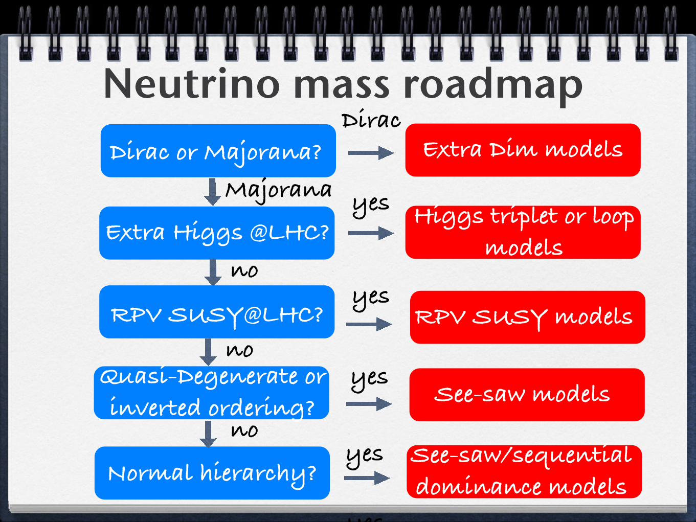
Neutrino mass roadmap

yesyes

Dirac or Majorana? Extra Dim models

See-saw modelsQuasi-Degenerate or inverted ordering?

Normal hierarchy?

Higgs triplet or loop models

Extra Higgs @LHC?

Dirac

yes

yes

Majorana

no

noSee-saw/sequential dominance models

RPV SUSY@LHC?

yes

RPV SUSY modelsno

yes

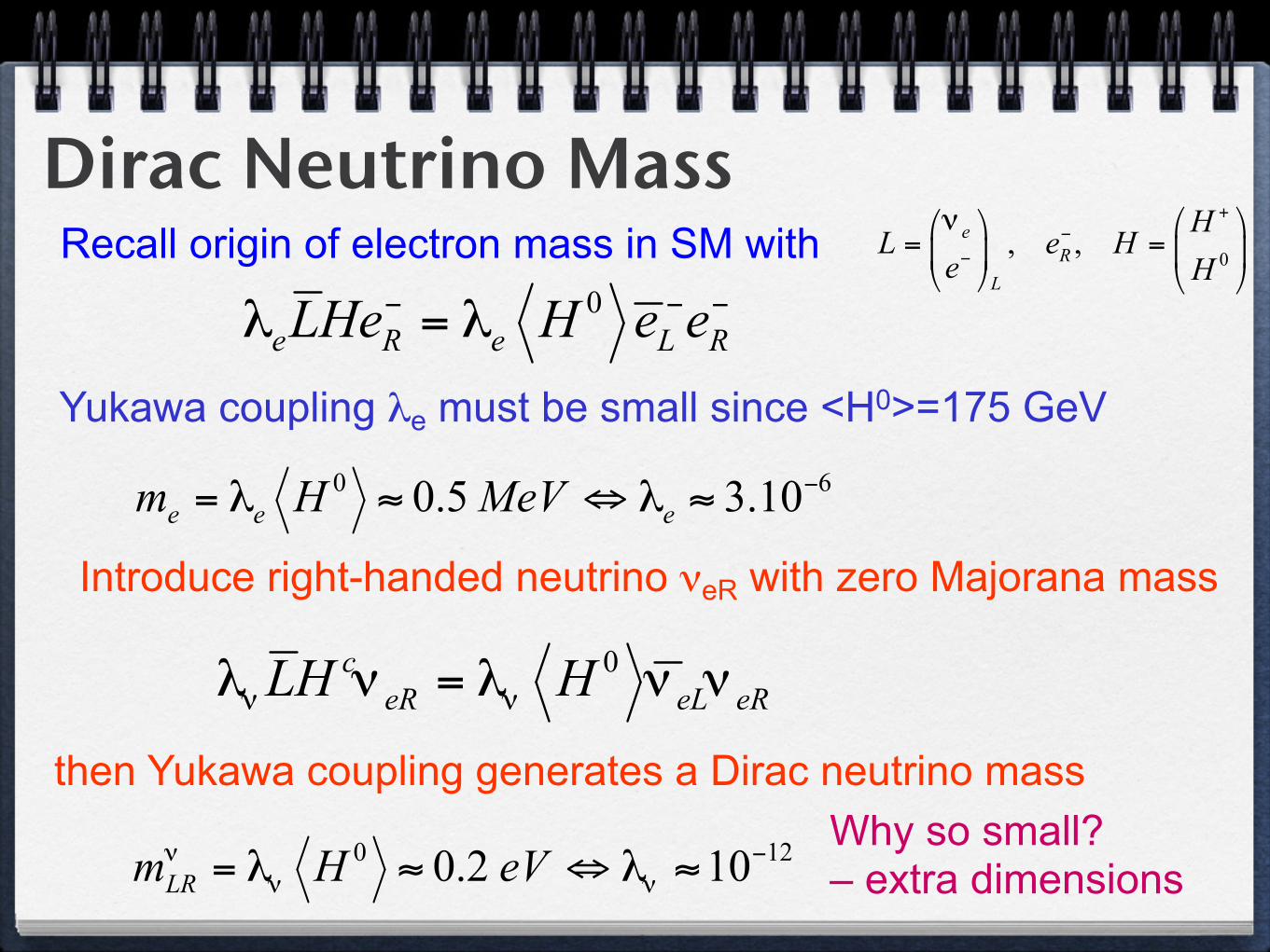
Yukawa coupling λe must be small since <H0>=175 GeV

Introduce right-handed neutrino νeR with zero Majorana mass

then Yukawa coupling generates a Dirac neutrino mass

Recall origin of electron mass in SM with

Why so small? – extra dimensions

Dirac Neutrino Mass

Flat extra dimensions with RH neutrinos in the bulk

Number of extra dimensions

e.g. for one extra dimension y the νR wavefunction spreads out over the extra dimension, leading to a volume suppressed Yukawa coupling at y=0

νR in bulk

Dienes, Dudas, Gherghetta; Arkhani-Hamed, Dimopoulos, Dvali, March-Russell

Warped extra dimensions with SM in the bulk

TeV brane

Planck brane

Overlap wavefunction of fermions with Higgs gives exponentially suppressed Dirac masses, depending on the fermion profiles

Majorana Neutrino Mass

Non-renormalisable ΔL =2 operator

where Δ is light Higgs triplet with VEV < 8GeV from ρ parameter

This is nice because it gives naturally small Majorana neutrino masses mLL» <H0>2/M where M is some high energy scale

The high mass scale can be associated with some heavy particle of mass M being exchanged (can be singlet or triplet)

Weinberg

Renormalisable ΔL =2 operator

See-saw mechanisms

Zee (one loop) Babu (two loop)

Extra scalars with couplings to leptons

Loop Models

Recent Loop Models

Figure 1: Tree-level and radiative seesaw mechanisms.

exists no such study in the literature with the focus put on the neutrino sector in radiativemodels, and we aim to start this enterprise by a study devoted to the RGEs of the Ma-

model. Naturally, this could be extended to other radiative models for neutrino masses,such as the Zee-Babu model [25, 26] or the Aoki-Kanemura-Seto model [27, 28]. In par-

ticular the interplay between the scalar and the lepton sectors has the potential to revealinteresting new e!ects, as we will already see in this study.

However, we want to stress that several studies are already available which investigate

e.g. limiting cases of our framework or subsets (or generalizations of subsets) of certainsectors of the Ma-model. A particular example for such a case would be the investigations

of the RGEs of a general Two Higgs Doublet Model (THDM). Whenever applicable inthis paper, we will refer to the corresponding works treating these related frameworks.

This paper is organized as follows: In Sec. 2, we review Ma’s scotogenic model anddiscuss the di!erent e!ective theories arising when subsequently integrating out the heavyneutrino fields. Next, in Sec. 3, we discuss in detail the matching conditions at the

boundaries between the respective theories, which in our case have to be consistentlyimposed at 1-loop level. Our main results, the explicit RGEs at 1-loop level are presented

in Sec. 4. After that, we present a numerical exemplifying study (in a slightly simplifiedframework) in Sec. 5, in order to illustrate how to use our results. We finally conclude in

Sec. 6.

2 Ma’s scotogenic model

The so-called scotogenic model has been discussed by Ma [24], and in the following we willtherefore call it Ma-model for simplicity. In this section, we will first review this model,

and then discuss some of its low-energy limits, which we will also use in our calculationslater on.

2

2

!++

W! W!

H0/A0

H+1,2 H+

1,2

"a "b

#+a #+

b

FIG. 1: The Cocktail Diagram

tests (EWPT) and collider searches, and we comment onpossible consequences for neutrinoless double beta de-cay (0!""). We then briefly discuss future detectionprospects, before concluding.

II. A MODEL FOR NEUTRINO MASSES.

In addition to the SM fields, the model includes twoSU(2)L singlet scalars (singly and doubly charged) S+

and #++, and a scalar doublet !2. We introduce a Z2

symmetry under which the !2 and S+ fields are odd,whereas #++ and the SM fields are even. The Z2 sym-metry should be unbroken after EW symmetry breaking,so that the lightest Z2-odd state remains stable and canprovide a dark matter particle candidate. Given the sym-metry and particle content of the model, the lagrangianwill include the following relevant terms leading to leptonnumber violation

!"L =$5

2

!

!†1!2

"2

+ %1 !T2 i&2!1 S

! + %2 #++S!S!

+'s !T2 i&2!1 S

+ #!! + Cab lcRalRb

#++ + h.c.. (1)

The SM scalar doublet !1 and the inert scalar doublet!2 can in the unitary gauge be written as

!1 =1"2

#

0h

$

+

#

0v

$

, !2 =1"2

#

#+

H0 + i A0

$

, (2)

where v # 174 GeV is the vacuum expectation value of!1. After EW symmetry breaking, and for %1 $= 0, thecharged states #+ and S+ will mix (the mixing anglebeing "), giving rise to two charged mass eigenstates

H+1 = s! S

+ + c! #+, H+

2 = c! S+ ! s! #

+, (3)

with s! , c! = sin", cos" respectively.The lagrangian in Eq. (1) breaks lepton number explic-

itly by two units [9], which generates a Majorana mass

for the left-handed neutrinos. The Z2 symmetry pre-cisely forbids all terms that would have generated neu-trino masses at either 1 or 2-loop order, and thereforethe leading contributions to neutrino masses appear at 3-loops through the ‘Cocktail Diagram’ shown in Figure 1.In the basis where the charged current interactions are

flavour-diagonal, the charged leptons e, µ, ( being thenmass eigenstates, and after summing up the contributionsfrom the six di$erent finite 3-loop diagrams in Figure 1(coming from H+

1,2, A0 and H0 running in the loop), theMajorana neutrino mass matrix reads:

m"ab # Cab xa xb s22!

I"

(16 )2)3A , (4)

where s2! = sin(2"), xa = ma/v for a = e, µ, ( , and

A =("m2

+)2 "m2

0

µ0 µ+

(%2 + 'sv)

m2# v2

. (5)

The factor I" is a dimensionless O(1) number emergingfrom the 3-loop integral after all generic factors have beenfactorized out. Its exact value depends on the specificmass spectrum, and we have estimated its value usingthe numerical code SecDec [10]. The reduced masses areµ!10 = m!1

H0+m!1

A0and µ!1

+ = m!1H1

+m!1H2

.The dependence of m"

ab on the mass di$erences"m20 =

m2A0

!m2H0

and "m2+ = m2

H2!m2

H1signals a GIM-like

mechanism at play in Eq. (4), which can be easily under-stood noticing that "m2

0 % $5 and "m2+ % %1. In the

limit $5 & 0 the lagrangian in Eq. (1) conserves leptonnumber and no Majorana neutrino mass can be gener-ated, while in the limit %1 & 0, the leading contributionto m"

ab will appear at a higher loop order.

We now analyze the ability of the model to reproducethe observed pattern of neutrino masses and mixings.The standard parametrization for the neutrino mass ma-trix in terms of three masses m1,2,3, three mixing angles*12, *23, *13 and three phases +, ,1, ,2 reads

m" = UT m"D U with m"

D = Diag (m1,m2,m3) (6)

U = Diag!

ei$1/2, ei$2/2, 1"

'%

&

c13c12 !c23s12!s23c12s13ei% s23s12!c23c12s13ei%

c13s12 c23c12!s23s12s13ei% !s23c12!c23s12s13ei%

s13e!i% s23c13 c23c13

'

(

with sij ( sin(*ij) and cij ( cos(*ij). A global fit toneutrino oscillation data after the recent measurementof *13 (see for example [11]) gives "m2

21 ( m22 ! m2

1 =7.62+0.19

!0.19' 10!5eV2,)

)"m231

)

) ()

)m23 !m2

1

)

) = 2.55+0.06!0.09'

10!3eV2, s212 = 0.320+0.016!0.017, s213 = 0.025+0.003

!0.003, ands223 = 0.43+0.03

!0.03 (0.61+0.02!0.04) if in the first (second) oc-

tant for *23. Neutrino oscillations are not sensitive tothe Majorana phases ,1 and ,2 nor to the absolute neu-trino mass scale, while the value of the CP phase + isbeyond current experimental sensitivity. In the inverted

Ma’s Scotogenic model

Cocktail model Gustafsson, No, Rivera

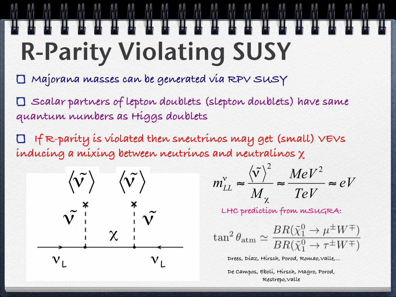
Majorana masses can be generated via RPV SUSY

Scalar partners of lepton doublets (slepton doublets) have same quantum numbers as Higgs doublets

If R-parity is violated then sneutrinos may get (small) VEVs inducing a mixing between neutrinos and neutralinos χ

Drees, Diaz, Hirsch, Porod, Romao,Valle,…

LHC prediction from mSUGRA:

De Campos, Eboli, Hirsch, Magro, Porod, Restrepo,Valle

R-Parity Violating SUSY

Dirac matrixPossible type II contribution

P.Minkowski, PLB67(1977)421

Neutrinos are light because RH neutrinos are heavy

No explanation of neutrino mixing without further ingredients

See-saw mechanisms

Mv = mLR.1

MRR.mT

LR

Heavy Majorana matrix

Light Majorana matrix

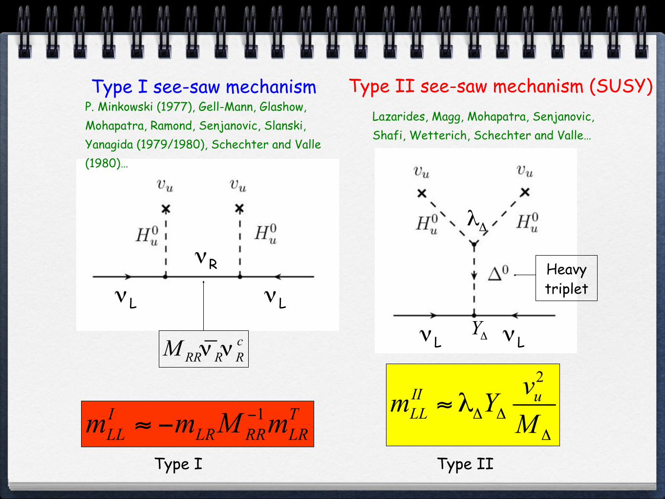
Type I see-saw mechanism Type II see-saw mechanism (SUSY)

Heavy triplet

Type II Type I

P. Minkowski (1977), Gell-Mann, Glashow, Mohapatra, Ramond, Senjanovic, Slanski, Yanagida (1979/1980), Schechter and Valle (1980)…

Lazarides, Magg, Mohapatra, Senjanovic, Shafi, Wetterich, Schechter and Valle…

Type III see-saw mechanism

Type III

Foot, Lew, He, Joshi; Ma…Supersymmetric adjoint SU(5)

SU(2)L fermion triplet

Perez et al; Cooper, SFK, Luhn,…

See-saw mechanisms with extra singlets S

Inverse see-saw

Linear see-saw

Wyler, Wolferstein; Mohapatra, Valle

Malinsky, Romao, Valle

M ≈ TeVèLHC

LFV predictions

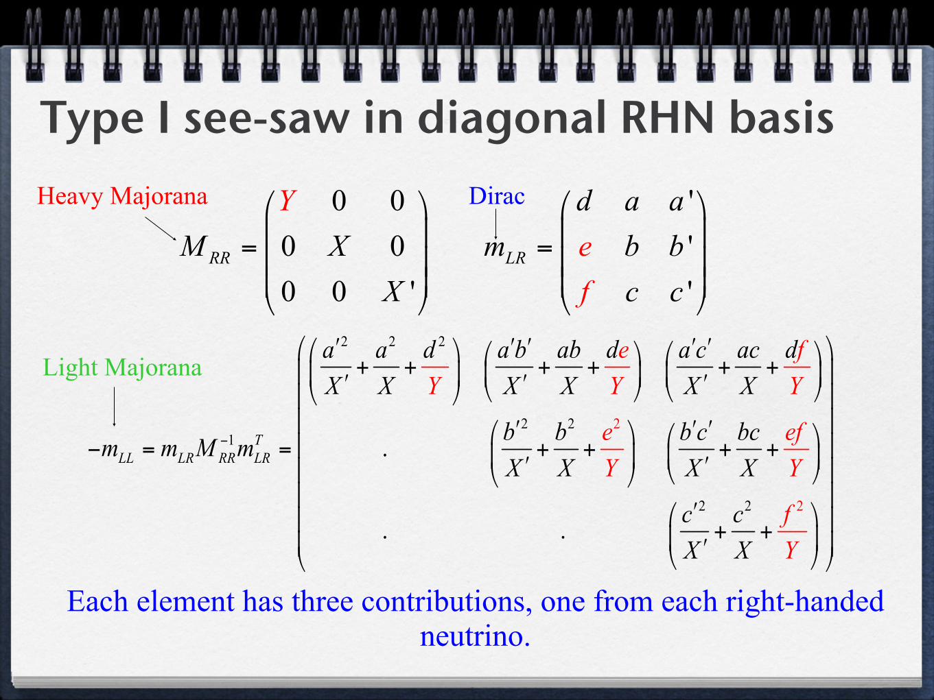
Type I see-saw in diagonal RHN basis

Each element has three contributions, one from each right-handed neutrino.

Heavy Majorana Dirac

Light Majorana

Sequential Dominance1. Ignore primed terms

2. Red terms dominate

3. Set d=0

Predicts a normal hierarchy

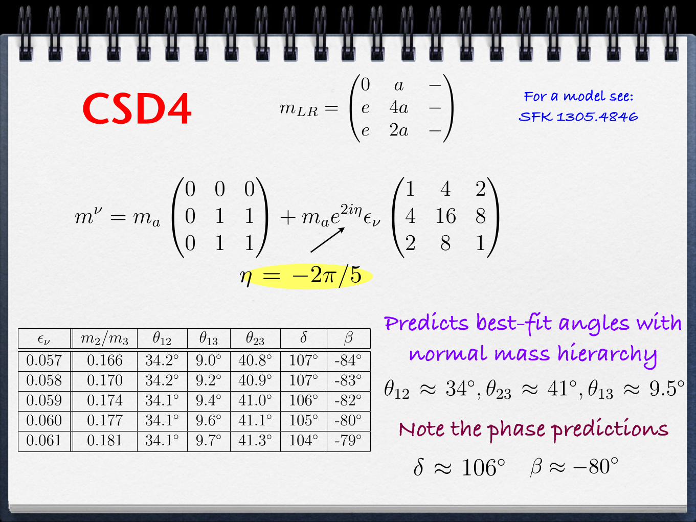
For example (CSD4):

f = e, b = 4a, c = 2a

m1 � m2 � m3 tan θ23 ≈ e/fm2 ∼ (a+ b+ c)2/X

m3 ∼ (d+ e+ f)2/Y

tan θ12 ≈√2a/(b− c)

θ13 ≈ O(m2/m3)

tan θ23 ≈ 1tan θ12 ≈ 1/

√2

Not bad!

�ν m2/m3 θ12 θ13 θ23 δ β

0.057 0.166 34.2◦

9.0◦

40.8◦

107◦

-84◦

0.058 0.170 34.2◦

9.2◦

40.9◦

107◦

-83◦

0.059 0.174 34.1◦

9.4◦

41.0◦

106◦

-82◦

0.060 0.177 34.1◦

9.6◦

41.1◦

105◦

-80◦

0.061 0.181 34.1◦

9.7◦

41.3◦

104◦

-79◦

Table 2: The predictions for PMNS parameters and m2/m3 arising from CSD4 as a function of �ν .Note that these predictions assume η = −2π/5. The predictions are obtained numerically using theMixing Parameter Tools package based on [15]. The leading order analytic results are not reliable asdiscussed in Appendix B.

mνin Eq.13 is a sum of two terms, the first being proportional to AAT ∝ �ϕν3��ϕν3�T

and the second being proportional to BBT ∝ �ϕν4��ϕν4�T . Since �ϕν1� ∝ (2,−1, 1)T is

orthogonal to both �ϕν3� and �ϕν4� it is then clearly annihilated by the neutrino mass

matrix, i.e. it is an eigenvector with zero eigenvalue. Therefore we immediately expect

mνin Eq.13 to be diagonalised by the TM1 mixing matrix [20] where the first column

is proportional to �ϕν1� ∝ (2,−1, 1)T . Therefore we already know that CSD4 must lead

to TM1 mixing exactly to all orders according to this general argument.

Exact TM1 mixing angle and phase relations are obtained by equating moduli of

PMNS elements to those of the first column of the TB mixing matrix:

c12c13 =

�2

3, (16)

|c23s12 + s13s23c12eiδ| = 1√

6, (17)

|s23s12 − s13c23c12eiδ| = 1√

6. (18)

From Eq.16 we see that TM1 mixing approximately preserves the successful TB mixing

for the solar mixing angle θ12 ≈ 35◦as the correction due to a non-zero but rela-

tively small reactor angle is of second order. While general TM1 mixing involves an

undetermined reactor angle θ13, we emphasise that CSD4 fixes this reactor angle. The

approximate leading order result is

θ13 ≈4

3√2

m2

m3. (19)

However the leading order results are not highly accurate and numerically the prediction

for the reactor angle depends on the phase η. For η = −2π/5 the reactor angle is in the

correct range as shown in Table 2.

In an approximate linear form, the relations in Eq.16-18 imply the atmospheric sum

rule relation,

θ23 ≈ 45◦+

√2θ13 cos δ. (20)

7

For η = −2π/5 the predictions shown in Table 2 for the small deviations of the at-

mospheric angle from maximality are well described by the sum rule in Eq.20. In the

present model this sum rule is satisfied by particular predicted values of angles and CP

phase which only depend on the neutrino mass ratio m2/m3. Over the successful range

of m2/m3 we predict CP violation with δ ≈ 106◦ and θ23 ≈ 41◦ which satisfy the sum

rule. Note that according to this sum rule, non-maximal atmospheric mixing is linked

to non-maximal CP violation.

3 Conclusions

There is long history of attempts to explain the neutrino mixing angles starting from

the type I see-saw mechanism and using SD, first using CSD to account for TB mix-

ing, then using CSD2 to obtain a small reactor angle before going to CSD3 where the

correct reactor angle can be reproduced along with maximal atmospheric mixing. We

have discussed a minimal predictive see-saw model based on CSD4 in which the right-

handed neutrino mainly responsible for the atmospheric neutrino mass has couplings

to (νe, νµ, ντ ) proportional to (0, 1, 1) and the right-handed neutrino mainly responsible

for the solar neutrino mass has couplings to (νe, νµ, ντ ) proportional to (1, 4, 2), with a

relative phase η = −2π/5. We have shown how these patterns of couplings and phase

could arise from an A4 family symmetry model of leptons.

We remark that the type of model presented here is referred to as “indirect” according

to the classification scheme of models in [4], meaning that the family symmetry is

completely broken by flavons and its only purpose is to generate the desired vacuum

alignments. By contrast, the “direct” models where the symmetries of the neutrino

and charged lepton mass matrices is identified as a subgroup of the family symmetry,

requires rather large family symmetry groups in order to account for the reactor angle

[21]. It is possible to have “semi-direct” models, either at leading order or emerging due

to higher order corrections [4], but these are inherently less predictive. In the light of the

observed reactor angle, “indirect models” therefore offer the prospect of full predictivityat the leading order from a small family symmetry group. Spontaneous CP violation

seems to be an important ingredient in the “indirect” approach since a particular phase

relation between flavons a crucial requirement.

The particular indirect model presented here, in which CSD4 emerges from an A4

family symmetry, offers a highly predictive framework involving only one free parameter

which is used to fix the neutrino mass ratio m2/m3, together with an overall neutrino

mass scale which is used to fix the atmospheric neutrino mass m3. Remarkably, the

model then predicts the PMNS angles θ12 ≈ 34◦, θ23 ≈ 41◦, θ13 ≈ 9.5◦, which exactly

coincide with the current best fit values for a normal neutrino mass hierarchy, together

with the distinctive prediction for the CP violating oscillation phase δ ≈ 106◦. These

predictions will surely be tested by current and planned high precision neutrino oscilla-

8

Predicts best-fit angles with normal mass hierarchy

For η = −2π/5 the predictions shown in Table 2 for the small deviations of the at-

mospheric angle from maximality are well described by the sum rule in Eq.20. In the

present model this sum rule is satisfied by particular predicted values of angles and CP

phase which only depend on the neutrino mass ratio m2/m3. Over the successful range

of m2/m3 we predict CP violation with δ ≈ 106◦ and θ23 ≈ 41◦ which satisfy the sum

rule. Note that according to this sum rule, non-maximal atmospheric mixing is linked

to non-maximal CP violation.

3 Conclusions

There is long history of attempts to explain the neutrino mixing angles starting from

the type I see-saw mechanism and using SD, first using CSD to account for TB mix-

ing, then using CSD2 to obtain a small reactor angle before going to CSD3 where the

correct reactor angle can be reproduced along with maximal atmospheric mixing. We

have discussed a minimal predictive see-saw model based on CSD4 in which the right-

handed neutrino mainly responsible for the atmospheric neutrino mass has couplings

to (νe, νµ, ντ ) proportional to (0, 1, 1) and the right-handed neutrino mainly responsible

for the solar neutrino mass has couplings to (νe, νµ, ντ ) proportional to (1, 4, 2), with a

relative phase η = −2π/5. We have shown how these patterns of couplings and phase

could arise from an A4 family symmetry model of leptons.

We remark that the type of model presented here is referred to as “indirect” according

to the classification scheme of models in [4], meaning that the family symmetry is

completely broken by flavons and its only purpose is to generate the desired vacuum

alignments. By contrast, the “direct” models where the symmetries of the neutrino

and charged lepton mass matrices is identified as a subgroup of the family symmetry,

requires rather large family symmetry groups in order to account for the reactor angle

[21]. It is possible to have “semi-direct” models, either at leading order or emerging due

to higher order corrections [4], but these are inherently less predictive. In the light of the

observed reactor angle, “indirect models” therefore offer the prospect of full predictivityat the leading order from a small family symmetry group. Spontaneous CP violation

seems to be an important ingredient in the “indirect” approach since a particular phase

relation between flavons a crucial requirement.

The particular indirect model presented here, in which CSD4 emerges from an A4

family symmetry, offers a highly predictive framework involving only one free parameter

which is used to fix the neutrino mass ratio m2/m3, together with an overall neutrino

mass scale which is used to fix the atmospheric neutrino mass m3. Remarkably, the

model then predicts the PMNS angles θ12 ≈ 34◦, θ23 ≈ 41◦, θ13 ≈ 9.5◦, which exactly

coincide with the current best fit values for a normal neutrino mass hierarchy, together

with the distinctive prediction for the CP violating oscillation phase δ ≈ 106◦. These

predictions will surely be tested by current and planned high precision neutrino oscilla-

8

For a model see: SFK 1305.4846

where vatm ≈ vsol.

The above charge assignments allow higher order non-renormalisable mixed terms

such as

∆WR ∼ 1

Λ(φatm.φsol)NatmNsol , (11)

which contribute off-diagonal terms to the right-handed neutrino mass matrix of a mag-

nitude which depends on the absolute scale of the flavon vevs �φatm� and �φsol� compared

to �ξatm� and �ξsol�. If all flavon vevs and messenger scales are set equal then these terms

are suppressed by � ∼ λ2according to the estimate below Eq.6, however they may be

even more suppressed. We shall ignore the contribution of such off-diagonal mass terms

in the following.

Implementing the see-saw mechanism, the effective neutrino mass matrix has the

form,

mν ∼ v

22

Λ2

��φatm��φatm�T

�ξatm�+

�φsol��φsol�T

�ξsol�

�, (12)

where v2 = �H2�. Hence it can be parameterised, up to an overall irrelevant phase, as,

mν= ma

0 0 0

0 1 1

0 1 1

+mae2iη�ν

1 4 2

4 16 8

2 8 1

(13)

where ma and �ν are real mass parameters which determine the physical neutrino masses

m3 and m2 and we written the relative phase difference between the two terms as 2η.Using Eq.10 the see-saw mechanism naturally leads to the neutrino mass matrix in

Eq.13 with �ν ≈ 2/21 ≈ 0.1. Hence the desired value of �ν ≈ 0.06 assumed below is not

unreasonable, and may be achieved for example by taking MB ≈ 2MA. As discussed in

[13], we shall also require a special phase relation η = −2π/5 in order to achieve our

goal of predicting the best fit values of the lepton mixing angles.

The phase difference η = −2π/5 between flavon vevs can be obtained in the context

of spontaneous CP violation from discrete symmetries as discussed in [12], and we shall

follow the strategy outlined there. The basic idea is to impose CP conservation on the

theory so that all couplings and masses are real. Note that the A4 assignments in Table 1

do not involve the complex singlets 1�, 1

��or any complex Clebsch-Gordan coefficients so

that the definition of CP is straightforward in this model and hence CP may be defined

in different ways which are equivalent for our purposes (see [12] for a discussion of this

point). The CP symmetry is broken in a discrete way by the form of the superpotential

terms. We shall follow [12] and suppose that the flavon vevs �φatm� and �φsol� to be real

with the phase η in Eq.13 originating from the solar right-handed neutrino mass due to

the flavon vev �ξsol� ∼ MBe4iπ/5

having a complex phase of 4π/5, while the flavon vev

5

�ν m2/m3 θ12 θ13 θ23 δ β

0.057 0.166 34.2◦

9.0◦

40.8◦

107◦

-84◦

0.058 0.170 34.2◦

9.2◦

40.9◦

107◦

-83◦

0.059 0.174 34.1◦

9.4◦

41.0◦

106◦

-82◦

0.060 0.177 34.1◦

9.6◦

41.1◦

105◦

-80◦

0.061 0.181 34.1◦

9.7◦

41.3◦

104◦

-79◦

Table 2: The predictions for PMNS parameters and m2/m3 arising from CSD4 as a function of �ν .Note that these predictions assume η = −2π/5. The predictions are obtained numerically using theMixing Parameter Tools package based on [15]. The leading order analytic results are not reliable asdiscussed in Appendix B.

mνin Eq.13 is a sum of two terms, the first being proportional to AAT ∝ �ϕν3��ϕν3�T

and the second being proportional to BBT ∝ �ϕν4��ϕν4�T . Since �ϕν1� ∝ (2,−1, 1)T is

orthogonal to both �ϕν3� and �ϕν4� it is then clearly annihilated by the neutrino mass

matrix, i.e. it is an eigenvector with zero eigenvalue. Therefore we immediately expect

mνin Eq.13 to be diagonalised by the TM1 mixing matrix [20] where the first column

is proportional to �ϕν1� ∝ (2,−1, 1)T . Therefore we already know that CSD4 must lead

to TM1 mixing exactly to all orders according to this general argument.

Exact TM1 mixing angle and phase relations are obtained by equating moduli of

PMNS elements to those of the first column of the TB mixing matrix:

c12c13 =

�2

3, (16)

|c23s12 + s13s23c12eiδ| = 1√

6, (17)

|s23s12 − s13c23c12eiδ| = 1√

6. (18)

From Eq.16 we see that TM1 mixing approximately preserves the successful TB mixing

for the solar mixing angle θ12 ≈ 35◦as the correction due to a non-zero but rela-

tively small reactor angle is of second order. While general TM1 mixing involves an

undetermined reactor angle θ13, we emphasise that CSD4 fixes this reactor angle. The

approximate leading order result is

θ13 ≈4

3√2

m2

m3. (19)

However the leading order results are not highly accurate and numerically the prediction

for the reactor angle depends on the phase η. For η = −2π/5 the reactor angle is in the

correct range as shown in Table 2.

In an approximate linear form, the relations in Eq.16-18 imply the atmospheric sum

rule relation,

θ23 ≈ 45◦+

√2θ13 cos δ. (20)

7

Note the phase predictions

β ≈ −80◦

mLR =

0 a −e 4a −e 2a −

CSD4

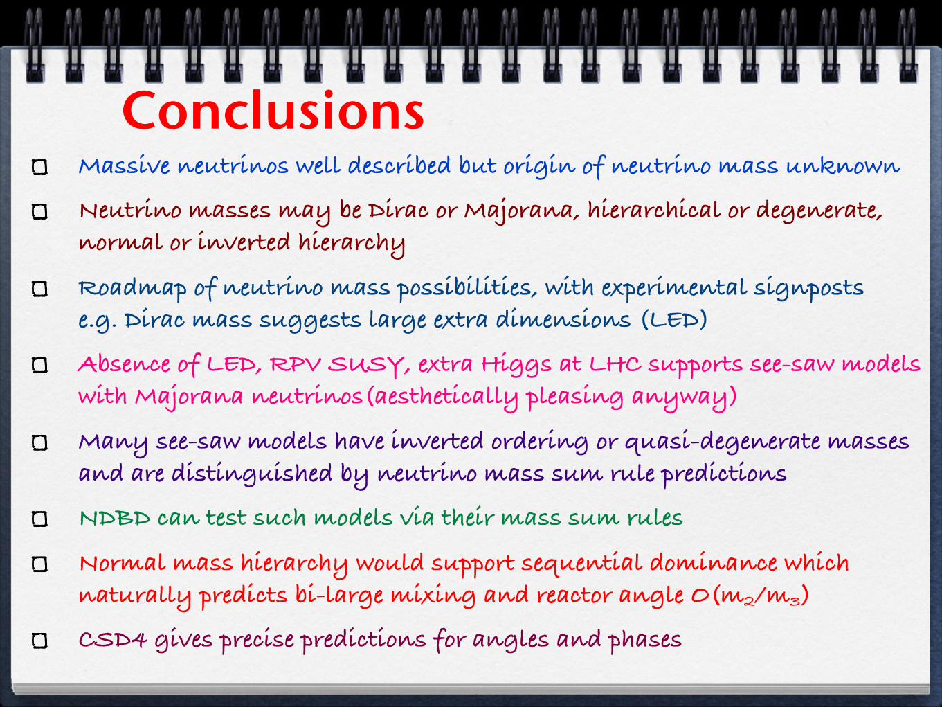
ConclusionsMassive neutrinos well described but origin of neutrino mass unknown

Neutrino masses may be Dirac or Majorana, hierarchical or degenerate, normal or inverted hierarchy

Roadmap of neutrino mass possibilities, with experimental signposts e.g. Dirac mass suggests large extra dimensions (LED)

Absence of LED, RPV SUSY, extra Higgs at LHC supports see-saw models with Majorana neutrinos(aesthetically pleasing anyway)

Many see-saw models have inverted ordering or quasi-degenerate masses and are distinguished by neutrino mass sum rule predictions

NDBD can test such models via their mass sum rules

Normal mass hierarchy would support sequential dominance which naturally predicts bi-large mixing and reactor angle O(m2/m3)

CSD4 gives precise predictions for angles and phases