description of a model to compute the aggregate

NTIA TECHNICAL MEMORANDUM 09-461

DESCRIPTION OF A MODEL TO COMPUTE THE AGGREGATE INTERFERENCE FROM

RADIO LOCAL AREA NETWORKS EMPLOYING DYNAMIC FREQUENCY

SELECTION TO RADARS OPERATING IN THE 5 GHz FREQUENCY RANGE

U.S. DEPARTMENT OF COMMERCE • National Telecommunications and Information Administration

NTIA TECHNICAL MEMORANDUM 09-461

DESCRIPTION OF A MODEL TO COMPUTE THE AGGREGATE INTERFERENCE FROM

RADIO LOCAL AREA NETWORKS EMPLOYING DYNAMIC FREQUENCY

SELECTION TO RADARS OPERATING IN THE 5 GHz FREQUENCY RANGE

Edward F. Drocella

Larry Brunson Charles T. Glass

U.S. DEPARTMENT OF COMMERCE Gary Locke, Secretary

Anna Gomez

Acting Assistant Secretary for Communications and Information

May 2009

ACKNOWLEDGMENTS

The authors wish to thank the federal and non-federal participants who assisted in the development of the analysis model documented in this technical memorandum. We would particularly like to thank the Department of Defense, whose technical expertise was critical to the completion of this model. We also greatly appreciate the insight of industry participants from many different manufacturing companies and service providers which proved invaluable in the development of this model.

ii

EXECUTIVE SUMMARY In 1997, the Federal Communications Commission (FCC) authorized the use of Unlicensed National Information Infrastructure (U-NII) devices in the 5150-5250 MHz, 5250-5350 MHz, and 5725-5825 MHz bands. The technical and operational requirements are different in each of these bands. Many of the devices presently operating under these rules are designed to meet the Institute of Electrical and Electronics Engineers (IEEE) 802.11(a) industry standard for wireless local area networks. The World Radiocommunication Conference 2003 (WRC-03) considered allocations for wireless access systems including unlicensed radio local area networks (RLANs), radar systems, and other services in the 5 GHz region of the spectrum. In preparing for WRC-03, the National Telecommunications and Information Administration (NTIA), in conjunction with the FCC, the Department of Defense, and the National Aeronautics and Space Administration, and working closely with industry, agreed to require U-NII devices operating in the 5250-5350 MHz and 5470-5725 MHz band to employ dynamic frequency selection (DFS), a listen-before-transmit mechanism. DFS works by selecting an alternate operating frequency for the U-NII device when a radar signal is detected above a minimum threshold. To determine the necessary DFS detection threshold, NTIA developed a computer model that calculated the aggregate interference level into a radar system from a population of RLANs. The model took into account RLAN transmit control of DFS to determine interference to four types of radar systems that operate in the 5 GHz frequency range. The types of radar included: ground-based scanning, ground-based tracking, airborne, and shipborne. Current and planned federal radar utilization of the 5 GHz frequency range was examined and characterized to study interactions between RLANs and the radars that operate at 5 GHz. Operational scenarios were developed that considered the operational deployments of unlicensed RLANs and typical deployments of radar systems representative of those that would operate in the band. These operational scenarios included physical placement factors, as well as technical characteristics of both the RLAN and radar systems. Link budget calculations were then performed to determine the effect of RLANs employing the DFS function and the aggregate level of RLAN signals that would be received by the different types of radar systems. The results of the NTIA analysis were used by the FCC to amend the Part 15 U-NII service rules. NTIA is in the process of developing a handbook documenting the best practices in spectrum engineering for use by regulators, technology developers, manufacturers, and service providers. This “Best Practices Handbook” will bring together a common set of approaches for conducting engineering analyses and will develop a common set of criteria for performing technical studies to evaluate emerging technologies. The objective of this technical memorandum is to document the analysis methodology that NTIA developed and used in assessing interference from RLANs to 5 GHz radar systems. NTIA will consider the analysis methodology and operational

iii

scenarios described in this technical memorandum as it develops the Best Practices Handbook.

iv

TABLE OF CONTENTS

SECTION 1.0 ................................................................................................................................... 1-1 INTRODUCTION............................................................................................................................ 1-1

1.1 BACKGROUND ......................................................................................................... 1-1 1.2 OBJECTIVE ................................................................................................................ 1-3 1.3 APPROACH ................................................................................................................ 1-3

SECTION 2.0 ................................................................................................................................... 2-1 DESCRIPTION OF RADAR USAGE IN THE 5 GHz FREQUENCY RANGE ........................... 2-1

2.1 INTRODUCTION ....................................................................................................... 2-1 2.2 RADARS OPERATING IN THE 5250-5350 MHz BAND........................................ 2-1 2.3 RADARS OPERATING IN THE 5470-5600 MHz BAND........................................ 2-1 2.4 RADARS OPERATING IN THE 5600-5650 MHz BAND........................................ 2-1 2.5 RADARS OPERATING IN THE 5650-5725 MHz BAND........................................ 2-2 2.6 SPECTRUM OCCUPANCY IN THE 5250-5725 MHz BAND................................. 2-2 2.7 ANTICIPATED FUTURE RADAR DEVELOPMEMT TRENDS AT 5 GHz.......... 2-2

SECTION 3.0 ................................................................................................................................... 3-1 DESCRIPTION OF OPERATIONAL SCENARIOS...................................................................... 3-1

3.1 INTRODUCTION ....................................................................................................... 3-1 3.2 DESCRIPTION OF RLAN DEPLOYMENT REGIONS ........................................... 3-1 3.3 DISTRIBUTION OF RLAN DEVICES TO BE ANALYZED .................................. 3-2 3.4 RADAR DELOYMENTS ........................................................................................... 3-3 3.5 RLAN AND RADAR LOCATION SETUP ............................................................... 3-5

SECTION 4.0 ................................................................................................................................... 4-1 RLAN AND RADAR TECHNICAL CHARACTERISTICS ......................................................... 4-1

4.1 INTRODUCTION ....................................................................................................... 4-1 4.2 RLAN TECHNICAL CHARACTERISTICS.............................................................. 4-1 4.3 RADAR TECHNICAL CHARACTERISTICS .......................................................... 4-2 4.4 PHYSICAL PARAMETER SETUP ........................................................................... 4-4

SECTION 5.0 ................................................................................................................................... 5-1 DESCRIPTION OF ANALYSIS MODEL...................................................................................... 5-1

5.1 INTRODUCTION ....................................................................................................... 5-1 5.2 ANALYSIS MODEL DESCRIPTION........................................................................ 5-1 5.3 DESCRIPTION OF ANALYSIS PARAMETERS ..................................................... 5-3 5.4 RADAR INTERFERENCE PROTECTION ............................................................... 5-9 5.5 INTERFERENCE CALCULATION PROCESS ...................................................... 5-10 5.6 DFS DETECTION THRESHOLD............................................................................ 5-12

SECTION 6.0 ................................................................................................................................... 6-1 RADAR SPECIFIC MODELING PARAMETERS ........................................................................ 6-1

6.1 INTRODUCTION ....................................................................................................... 6-1 6.2 GROUND-BASED SCANNING RADARS ............................................................... 6-1

v

6.3 GROUND-BASED TRACKING RADARS ............................................................... 6-1 6.4 SHIPBORNE RADARS .............................................................................................. 6-2 6.5 AIRBORNE RADARS................................................................................................ 6-3

SECTION 7.0 .............................................................................................................................. 7-1 SUMMARY ................................................................................................................................ 7-1

APPENDIX A: MATLAB CODE FOR 5 GHz MODEL ......................................................... A-1

vi

ACRONYMS AND ABBREVIATIONS

AP Access Point CDF Cumulative Distribution Function DFS Dynamic Frequency Selection DoD Department of Defense EIRP Equivalent Isotropically Radiated Power EMC Electromagnetic Compatibility FCC Federal Communications Commission FDR Frequency Dependent Rejection IEEE Institute for Electrical and Electronics Engineers IF Intermediate Frequency ITM Irregular Terrain Model ITU-R International Telecommunication Union-Radiocommunication Sector I/N Interference-to-Noise Ratio mW Milliwatts NTIA National Telecommunications and Information Administration Nch Number of Channels PDF Probability Density Function POC Probability of Coincidence RLAN Radio Local Area Network TDWR Terminal Doppler Weather Radar U-NII Unlicensed-National Information Infrastructure WECA Wireless Ethernet Compatibility Alliance Wi-Fi Wireless-Fidelity WRC-03 World Radiocommunication Conference 2003

vii

SECTION 1.0 INTRODUCTION

1.1 BACKGROUND The National Telecommunications and Information Administration (NTIA) is the Executive Branch agency principally responsible for developing and articulating domestic and international telecommunications policy. NTIA’s responsibilities include establishing policies concerning spectrum assignments, allocation in use, and providing various departments and agencies with guidance to ensure that their conduct of telecommunication activities is consistent with these policies.1 Accordingly, NTIA conducts technical studies and makes recommendations regarding telecommunications policies and presents executive branch views on telecommunications matters to the Congress, the Federal Communications Commission (FCC), and the public. NTIA is responsible for managing federal use of the radio frequency spectrum. The FCC is responsible for managing spectrum use by the private sector and state and local governments. In support of its responsibilities, NTIA has undertaken numerous spectrum-related studies to assess spectrum utilization, examine the feasibility of reallocating spectrum used by the federal government to private sector uses and relocating federal government systems, identify existing or potential electromagnetic compatibility (EMC) problems between systems, provide recommendations for resolving any EMC conflicts, and recommend changes to promote efficient and effective use of the radio frequency spectrum and to improve federal spectrum management procedures. In 1997, the FCC authorized the use of Unlicensed National Information Infrastructure (U-NII) devices in the 5150-5250 MHz, 5250-5350 MHz, and 5725-5825 MHz bands.2 The technical and operational requirements are different in each of these bands. Many of the devices presently operating under these rules are designed to meet the Institute of Electrical and Electronics Engineers (IEEE) 802.11(a) industry standard for wireless local area networks.3

On January 15, 2002, the Wireless-Fidelity (Wi-Fi) Alliance (formally referred to as the Wireless Ethernet Compatibility Alliance (WECA)) submitted a petition for rulemaking seeking an additional 255 MHz of spectrum for use by U-NII devices in the

1. National Telecommunications and Information Administration, U.S. Department of Commerce, Manual of Regulations and Procedures for Federal Radio Frequency Management (2008). 2. See Amendment of the Commission’s Rules to Provide for Operation of Unlicensed NII Devices in the 5 GHz Frequency Range, ET Docket 96-102, Report and Order, 12 FCC Rcd 1576 (1997) available at http://www.fcc.gov/Bureaus/Engineering_Technology/Orders/1997/fcc97005.pdf. 3. This is also referred to as a Wireless-Fidelity (Wi-Fi) standard.

1-1

5470-5725 MHz band.4 In its petition, WECA stated that additional spectrum was needed to accommodate growing demand for unlicensed radio local area networks (RLANs) capable of operating at data rates of up to 54 megabits per second. WECA also stated that their proposal to expand the spectrum available for U-NII devices would align the United States with the European allocations for High Performance RLANs, thereby permitting the use of common products in both the United States and Europe. The World Radiocommunication Conference 2003 (WRC-03) considered allocations for wireless access systems including RLANs, radar systems, and other services in the 5 GHz region of the spectrum. In preparing for WRC-03 NTIA, in conjunction with the FCC, the Department of Defense (DoD), and the National Aeronautics and Space Administration, and working closely with industry, agreed to require U-NII devices operating in the 5250-5350 MHz and 5470-5725 MHz band to employ dynamic frequency selection (DFS), a listen-before-transmit mechanism.5 DFS works by selecting an alternate frequency if a signal is detected at power levels above a certain threshold.6

To determine the necessary DFS detection thresholds, NTIA developed a computer model (5 GHz Model) that calculated the aggregate interference level into a radar system from a deployment of RLANs. The model took into account the RLAN transmit control of DFS to determine interference to four types of radar systems that operate in the 5 GHz frequency range. The types of radar included: ground-based scanning, ground-based tracking, airborne, and shipborne. Current and planned federal radar utilization of the 5 GHz frequency range was examined and characterized to study interactions between RLANs and the radars that operate at 5 GHz. NTIA developed scenarios that considered the operational deployment of unlicensed RLANs and typical deployments of radar systems representative of those that would operate in the band. These scenarios included physical placement factors as well as technical characteristics of both the RLAN and radar systems. Link budget calculations were then performed to determine the effect of RLANs employing the DFS function and the aggregate level of RLAN signals that would be received by the radar systems. The FCC used the results of the NTIA analysis to amend the Part 15 U-NII service rules.7

4. Wireless Ethernet Compatibility Alliance, Petition for Rulemaking To Permit Unlicensed National Information Infrastructure Devices to Operate in the 5.470-5.725 GHz Band, RM-10371 (Jan. 15, 2002). 5. Press Release, U.S. Department of Commerce, National Telecommunications and Information Administration, Agreement Reached Regarding U.S. Position on 5 GHz Wireless Access Devices (Jan. 31, 2003) available at http://www.ntia.doc.gov/ntiahome/press/2003/5ghzagreement.htm. 6. DFS is a mechanism that detects the presence of signals from other systems, such as radar systems, and avoids co-channel operation. 7. See Revision of Parts 2 and 15 of the Commission’s Rules to Permit Unlicensed National Information Infrastructure (U-NII) Devices in the 5 GHz Band, Order, ET Docket No. 03-122, 21 FCC Rcd 1816 (2006) available at http://fjallfoss.fcc.gov/edocs_public/attachmatch/DA-03-4096A1.pdf.

1-2

NTIA is in the process of developing a handbook documenting best practices in spectrum engineering for use by regulators, technology developers, manufacturers, and service providers. This “Best Practices Handbook” will bring together a common set of approaches for conducting engineering analyses and will develop a common set of criteria for performing technical studies to evaluate emerging technologies. 1.2 OBJECTIVE The objective of this technical memorandum is to document the analysis methodology NTIA developed to assess potential interference from RLANs to 5 GHz radar systems. The methodology and operational scenarios described in this technical memorandum will be considered in the Best Practices Handbook. 1.3 APPROACH

NTIA used the following approach in the development of the 5 GHz Model to assess aggregate interference to radar systems. 1. Describe radar usage in the 5 GHz frequency range 2. Describe operational scenarios for RLAN and radar systems a. urban, suburban, rural regions b. number and location of RLANs by region c. radar system deployments 3. Determine system characteristics for RLAN and radar systems

4. Develop interference analysis methodology consistent with accepted engineering procedures for performing electromagnetic compatibility (EMC) analyses including appropriate International Telecommunication Union-Radiocommunication Sector (ITU-R) recommendations to include:

a. interference power calculation b. propagation loss c. frequency dependent rejection d. antenna gain patterns e. interference criteria 5. Develop the 5 GHz Model using the interference analysis methodology

1-3

SECTION 2.0 DESCRIPTION OF RADAR USAGE IN THE 5 GHz

FREQUENCY RANGE 2.1 INTRODUCTION This section provides a description of the federal radar usage in the 5 GHz frequency bands, divided into four distinct frequency bands: 5250-5350 MHz, 5470-5600 MHz, 5600-5650 MHz, and 5650-5725 MHz. The spectral occupancy and the anticipated future development of radars in the 5250-5725 MHz frequency range are also discussed. 2.2 RADARS OPERATING IN THE 5250-5350 MHz BAND The federal radar systems operating in the 5250-5350 MHz band are primarily used by the military. These military radars have the operational capability to tune across the entire 5250-5725 MHz frequency range. The military radars that operate in this band include both target search and tracking radars that can use a single frequency or can employ frequency-hopping techniques across the entire band. In the past, these radars have been limited to operating on or near military installations. However, there may be situations where these radars may have to be used more widely in support of homeland security. One of the areas of concern in assessing interference to military radars regards future radar deployments and the expanding role of military radars in support of homeland defense. This expanded role could result in a requirement to deploy military radars in cities and metropolitan areas where RLANs are expected to have their highest usage. 2.3 RADARS OPERATING IN THE 5470-5600 MHz BAND The 5470-5600 MHz frequency band is used by marine radars for maritime navigation. The marine radar provides ships with surface search, navigation capabilities, and tracking services, particularly during inclement weather. These navigation radars are used by all categories of commercial and government vessels operating in U.S. waters, including foreign and U.S.-flagged cargo, oil tankers, and passenger ships. These radars are vital sensors for safe navigation of waterways. The marine navigation radar provides indications and data on surface craft, obstructions, buoy markers, and navigation marks to assist in navigation and collision avoidance. Emissions from maritime radionavigation radars are observable at distances of at least several kilometers inland. The radar emission levels are higher in the vicinity of the shoreline, on bridges near waterways, and on coastlines. 2.4 RADARS OPERATING IN THE 5600-5650 MHz BAND The 5600-5650 MHz band is used by Terminal Doppler Weather Radar (TDWR), which provides quantitative measurements of wind gusts, wind shear, micro bursts, and

2-1

other weather hazards for improving the safety of operations at major airports in the United States. In addition to TDWR, non-federal meteorological radars operate throughout the 5350-5625 MHz frequency range. In general, weather surveillance radars operate near populated areas and can be in close proximity to RLANs.

2.5 RADARS OPERATING IN THE 5650-5725 MHz BAND The radars that operate in the 5650-5725 MHz band are primarily military systems that are capable of tuning across the entire 5400-5900 MHz frequency range. The radars operating in this band segment can be either mobile or transportable and are used for surveillance and test range instrumentation. Test range instrumentation radars are used to provide highly accurate position data on space launch vehicles and aeronautical vehicles undergoing developmental and operational testing. Periods of operation can last from minutes up to 4-5 hours, depending upon the test program that is being supported. Operations are conducted at scheduled times 24 hours per day, 7 days a week. 2.6 SPECTRUM OCCUPANCY IN THE 5250-5725 MHz BAND NTIA performed spectrum occupancy measurements in the 5250-5725 MHz band near the cities of San Diego, Los Angles, San Francisco, and Denver.8 The activity in the 5250-5725 MHz band in all of these areas was found to be highly dynamic. Radar measurement personnel have noted that, during the past 25 years of spectrum survey measurements in the band 5250-5725 MHz, weather and diurnal cycles have had a strong effect on the levels of occupancy in the band. The measured spectral occupancy plots show that, in the frequency range between 5470-5725 MHz, the maximum observed signal levels are much higher as compared to levels in the 5250-5350 MHz band.9

2.7 ANTICIPATED FUTURE RADAR DEVELOPMEMT TRENDS AT 5 GHz As a result of reductions in the existing radiolocation service allocations in the lower frequency bands, it is likely that new radar systems will be developed that operate in this frequency range.10

8. National Telecommunications and Information Administration, NTIA Report 97-334, Broadband Spectrum Survey at San Diego, California (1996) (NTIA Report 97-334); National Telecommunications and Information Administration, NTIA Report 97-336, Broadband Spectrum Survey at Los Angeles, California (1997) (NTIA Report 97-336); National Telecommunications and Information Administration, NTIA Report 99-367, Broadband Spectrum Survey at San Francisco, California May-June 1995 (1999) (NTIA Report 99-367); National Telecommunications and Information Administration, NTIA Report 95-321, Broadband Spectrum Survey at Denver, Colorado (1995) (NTIA Report 95-321). 9. NTIA Report 99-367 at 69; NTIA Report 97-336 at 40; NTIA Report 97-334 at 50; and NTIA Report 95-321 at 48. 10. Spectrum reallocations under Title VI – Omnibus Budget Reconcilliation Act of 1993 and Title III of the Balanced Budget Act of 1997 reduced the radar spectrum allocations in the 1 to 3 GHz frequency range. See National Telecommunications and Information Administration, NTIA Special Publication 95-32, Spectrum Reallocation Final Report – Response to Title VI Omnubus Budget Reconcilliation Act of 1993

2-2

Advanced radar designs are tending toward increased use of modulated compressed-pulse waveforms. These approaches include various types of phase coding (e.g., Barker codes, minimum shift keying, etc.) and frequency modulation (e.g., chirping). Assuming that this trend toward incorporating more complex modulation schemes within the radar pulses continues, it can be expected that pulse lengths will increase. At this time, some 3 GHz radars are transmitting pulse lengths on the order of 100 microseconds and longer pulse lengths are foreseeable. Longer pulses will tend to increase the average power output of the advanced radar transmitters. The trend is also toward solid state power output devices that will have lower peak power levels, resulting in lower detected power in the receiver systems. The longer pulse lengths will have the effect of increasing the duty cycle of the radar system.

(1995) and National Telecommunications and Information Administration, NTIA Special Publication 98-36, Spectrum Reallocation Report – Response to Title III of the Balanced Budget Act of 1997 (1998).

2-3

SECTION 3.0 DESCRIPTION OF OPERATIONAL SCENARIOS

3.1 INTRODUCTION

This section describes the operational scenarios for the RLANs and the radars used in the 5 GHz Model to assess the potential aggregate interference to the radars operating in the 5 GHz frequency range. The RLAN deployment regions are first described, followed by an explanation of how the RLANs are distributed. The deployments for each category of radar are then described.

3.2 DESCRIPTION OF RLAN DEPLOYMENT REGIONS The 5 GHz Model distributes RLANs over three regions: urban, suburban, and rural. The urban region reflects the corporate and public access use of RLANs. The suburban region reflects corporate, public access, and home RLAN use. The rural region reflects only home RLAN use. The three regions are assumed to exist within concentric circles as shown in Figure 3-1. The locations of the RLANs within the three regions are determined randomly using a uniform probability distribution.

Urban

Suburban

Rural

Figure 3-1. RLAN Deployment Regions

3-1

Each of the individual regions would be expected to contain various types of structures, with maximum structure heights varying from one region to the next. This arrangement of the deployment regions represents the structure of a typical city, with a dense urban core containing structures with greater maximum heights, a less dense suburban region with structures of lesser height, and a more sparsely populated rural region consisting mostly of residential structures. Table 3-1 provides a listing of the parameters that must be defined in order to adequately describe the deployment regions.

Table 3-1. Parameters Describing the RLAN Deployment Regions

Parameter Description Urban Radius Distance from the center of the city to the

outer edge of the urban region Suburban Radius Distance from the center of the city to the

outer edge of the suburban region Rural Radius Distance from the center of the city to the

outer edge of the rural region Urban Height Maximum urban structure height where

RLAN may be located Suburban Height Maximum suburban structure height where

RLAN may be located Rural Height Maximum rural structure height where

RLAN may be located The antenna heights of the RLANs within the three regions are determined randomly within a pre-determined range of values using a uniform probability distribution. 3.3 DISTRIBUTION OF RLAN DEVICES TO BE ANALYZED To establish the sharing environment, it is important to build a representative model that defines the total number of co-channel RLANs within the environment where a particular radar in the 5 GHz frequency range could be deployed, and how the RLANs are expected to be deployed throughout the three regions. Table 3-2 provides a listing of the parameters that must be defined in order to adequately describe the RLAN distributions within these regions. 3.3.1 Determine the Total Number of Active RLANs Within the City Since centralized architectures, mesh networks, and ad-hoc networks (peer-to-peer) are all permissible in this band, it is appropriate to leave the number of RLANs as a variable. The value to be used should reflect the total population, market penetration rates, activity factors, and other factors as appropriate.

3-2

3.3.2 Determine the Relative Weights of Active RLANs Within Each Region The relative weight for each region describes the fraction of the total users that can be expected to be found in any one particular region (i.e., urban, suburban, or rural). The sum of the weights for each of these regions must equal 100 percent. The relative weights should consider the types of systems expected to be deployed within each of the regions (e.g., rural users would primarily be expected to be residential in nature, and thus would receive a lower relative weight than the urban region, where most uses could be expected to be of a corporate nature).

Table 3-2. Parameters Describing RLAN Device Distribution

Parameter Description Number of RLANs Total number of RLANs considered Urban Weighting Percentage of RLANs that are in the

urban region Suburban Weighting Percentage of RLANs that are in the

suburban region Rural Weighting Percentage of RLANs that are in the

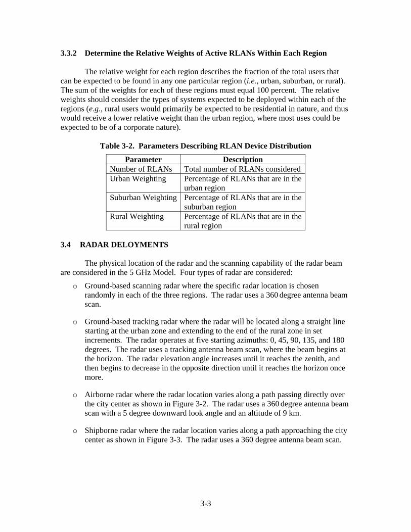
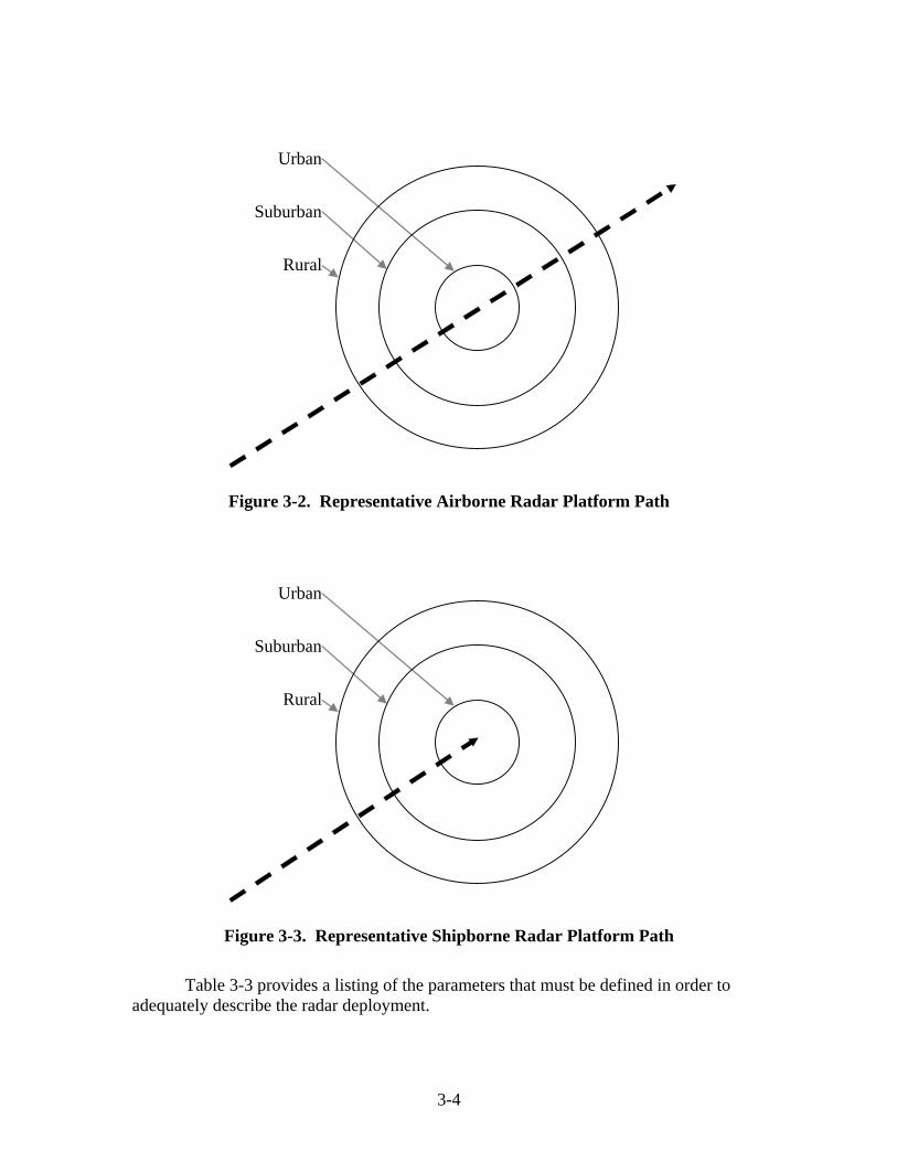
rural region 3.4 RADAR DELOYMENTS The physical location of the radar and the scanning capability of the radar beam are considered in the 5 GHz Model. Four types of radar are considered:

o Ground-based scanning radar where the specific radar location is chosen randomly in each of the three regions. The radar uses a 360 degree antenna beam scan.

o Ground-based tracking radar where the radar will be located along a straight line starting at the urban zone and extending to the end of the rural zone in set increments. The radar operates at five starting azimuths: 0, 45, 90, 135, and 180 degrees. The radar uses a tracking antenna beam scan, where the beam begins at the horizon. The radar elevation angle increases until it reaches the zenith, and then begins to decrease in the opposite direction until it reaches the horizon once more.

o Airborne radar where the radar location varies along a path passing directly over the city center as shown in Figure 3-2. The radar uses a 360 degree antenna beam scan with a 5 degree downward look angle and an altitude of 9 km.

o Shipborne radar where the radar location varies along a path approaching the city center as shown in Figure 3-3. The radar uses a 360 degree antenna beam scan.

3-3

Urban

Suburban

Rural

Figure 3-2. Representative Airborne Radar Platform Path

Urban

Suburban

Rural

Figure 3-3. Representative Shipborne Radar Platform Path

Table 3-3 provides a listing of the parameters that must be defined in order to

adequately describe the radar deployment.

3-4

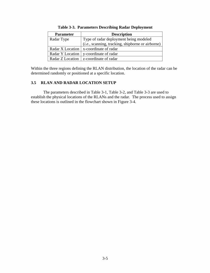
Table 3-3. Parameters Describing Radar Deployment

Parameter Description Radar Type Type of radar deployment being modeled

(i.e., scanning, tracking, shipborne or airborne) Radar X Location x-coordinate of radar Radar Y Location y-coordinate of radar Radar Z Location z-coordinate of radar

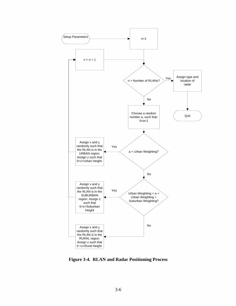
Within the three regions defining the RLAN distribution, the location of the radar can be determined randomly or positioned at a specific location. 3.5 RLAN AND RADAR LOCATION SETUP

The parameters described in Table 3-1, Table 3-2, and Table 3-3 are used to establish the physical locations of the RLANs and the radar. The process used to assign these locations is outlined in the flowchart shown in Figure 3-4.

3-5

Setup Parameters

n > Number of RLANs?

n=1

QuitChoose a random

number a, such that:0<a<1

a < Urban Weighting?

Assign x and yrandomly such thatthe RLAN is in the

URBAN region.Assign z such that0<z<Urban Height.

n = n + 1

Urban Weighting < a <Urban Weighting +

Suburban Weighting?


SUBURBANregion. Assign z

such that0<z<Suburban

Height


RURAL region.Assign z such that0 <z<Rural Height.

Assign type andlocation of

radar

Yes

No

Yes

No

Yes

No

Figure 3-4. RLAN and Radar Positioning Process

3-6

SECTION 4.0 RLAN AND RADAR TECHNICAL

CHARACTERISTICS 4.1 INTRODUCTION This section provides the system characteristics of the RLANs and the radar systems used in the 5 GHz Model. The RLAN technical characteristics used in the 5 GHz Model include: power levels for the different classes of RLAN devices, transmit and receive antenna azimuth and elevation gain patterns, and transmitter and receiver bandwidths. The radar technical characteristics used in the 5 GHz Model include: transmitter power, transmit and receive antenna azimuth and elevation gain patterns, receiver intermediate frequency (IF) bandwidth, receiver noise figure, and type of radar (e.g., scanning, tracking, airborne, or shipborne). 4.2 RLAN TECHNICAL CHARACTERISTICS 4.2.1 RLAN Power Levels RLAN devices used in different applications will have different power levels. The FCC Rules for U-NII devices permit a maximum equivalent isotropically radiated power (EIRP) level. However, because of battery and size limitations, EIRP levels lower than the maximum level permitted by the FCC can be employed. Since all of the RLANs in a given operational scenario will not have the same EIRP level, a distribution (i.e., a weighting) of the EIRP levels is necessary. The RLAN device EIRP levels and the fraction of devices operating at each level can be modified to analyze other operational scenarios. 4.2.2 RLAN Transmitter and Receiver Bandwidth The RLAN channel bandwidth is 20 MHz, however, the actual transmitter and receiver bandwidth is typically narrower (e.g., 18 MHz). 4.2.3 RLAN Antenna Gain Patterns The RLAN azimuth and elevation antenna patterns are defined in terms of the antenna gain in decibels relative to an isotropic antenna (dBi) as a function of the azimuth and elevation angles in degrees. The antenna patterns can be obtained from manufacturer data, from ITU-R recommendations, or defined by the user for a specific application.11

11. International Telecommunication Union-Radiocommunication Sector, Recommendation ITU-R F.1336, Reference Radiation Patterns of Omnidirectional and Other Antennas in Point-to-Multipoint Systems for Use in Sharing Studies (1997) (document available through agency).

4-1

4.3 RADAR TECHNICAL CHARACTERISTICS 4.3.1 Radar Transmitter and Receiver Characteristics

Representative technical and operational characteristics of the scanning, tracking,

and airborne radars used in the 5 GHz Model are provided in Recommendation ITU-R M.1638.12 For the shipborne radars, the technical characteristics in Recommendation ITU-R M.1313 are used in the 5 GHz Model.13 These ITU-R Recommendations provide the transmitter power level, mainbeam antenna gain, transmitter and receiver bandwidths, and receiver noise figure for each type of radar included in the model. Additional radars can be added to the model if necessary.

4.3.2 Radar Antenna Gain Patterns

A statistical gain antenna model is used to determine the radar antenna gain in the azimuth and elevation orientations.14 The model gives the antenna gain as a function of off-axis angle (θ) for a given main beam antenna gain (G). The model includes separate algorithms for very high-gain (G > 48 dBi), high-gain (22 < G < 48 dBi), and medium-gain (10 < G < 22 dBi) antennas. Figure 4-1 illustrates the general form of the antenna gain distribution. The equations for the angles θM (first side-lobe region), θR (near side-lobe region), and θB (far side-lobe region) are given in Table 4-1. The antenna gains, as a function of off-axis angle, are given in Table 4-2 for very high-gain antennas, in Table 4-3 for high-gain antennas, and in Table 4-4 for medium-gain antennas. The angle θ is in degrees and all gain values are given in terms of dBi.

B

12. International Telecommunication Union-Radiocommunication Sector, Recommendation ITU-R M.1638, Characteristics of and Protection Criteria for Radiolocation, Aeronautical Radionavigation and Meteorological Radars Operating in the Frequency Bands Between 5250 and 5850 MHz (2003) (document available through agency). 13. International Telecommunication Union-Radiocommunication Sector, Recommendation ITU-R M.1313-1, Technical Characteristics of Maritime Radionavigation Radars (2000) (document available through agency). 14. Joint Spectrum Center, JSC-CR-96-016B, JSMSW Interference Analysis Algorithms (1998) at 2-11.

4-2

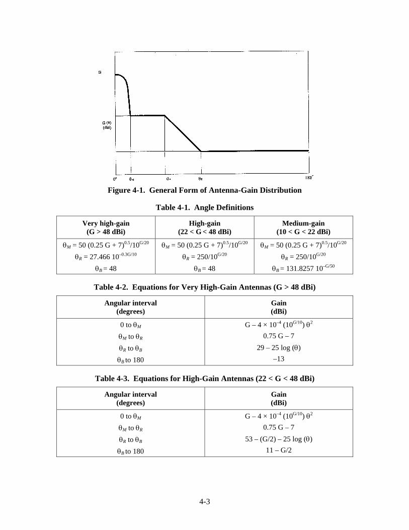
Figure 4-1. General Form of Antenna-Gain Distribution

Table 4-1. Angle Definitions

Very high-gain (G > 48 dBi)

High-gain (22 < G < 48 dBi)

Medium-gain (10 < G < 22 dBi)

θM = 50 (0.25 G + 7)0.5/10G/20

θR = 27.466 10–0.3G/10

θB = 48

θM = 50 (0.25 G + 7)0.5/10G/20

θR = 250/10G/20

θB = 48

θM = 50 (0.25 G + 7)0.5/10G/20

θR = 250/10G/20

θB = 131.8257 10–G/50

Table 4-2. Equations for Very High-Gain Antennas (G > 48 dBi)

Angular interval (degrees)

Gain (dBi)

0 to θM

θM to θR

θR to θB

θB to 180

G – 4 × 10–4 (10G/10) θ2

0.75 G – 7 29 – 25 log (θ)

–13

Table 4-3. Equations for High-Gain Antennas (22 < G < 48 dBi)


Gain (dBi)

0 to θM

θM to θR

θR to θB

θB to 180

G – 4 × 10–4 (10G/10) θ2

0.75 G – 7 53 – (G/2) – 25 log (θ)

11 – G/2

4-3

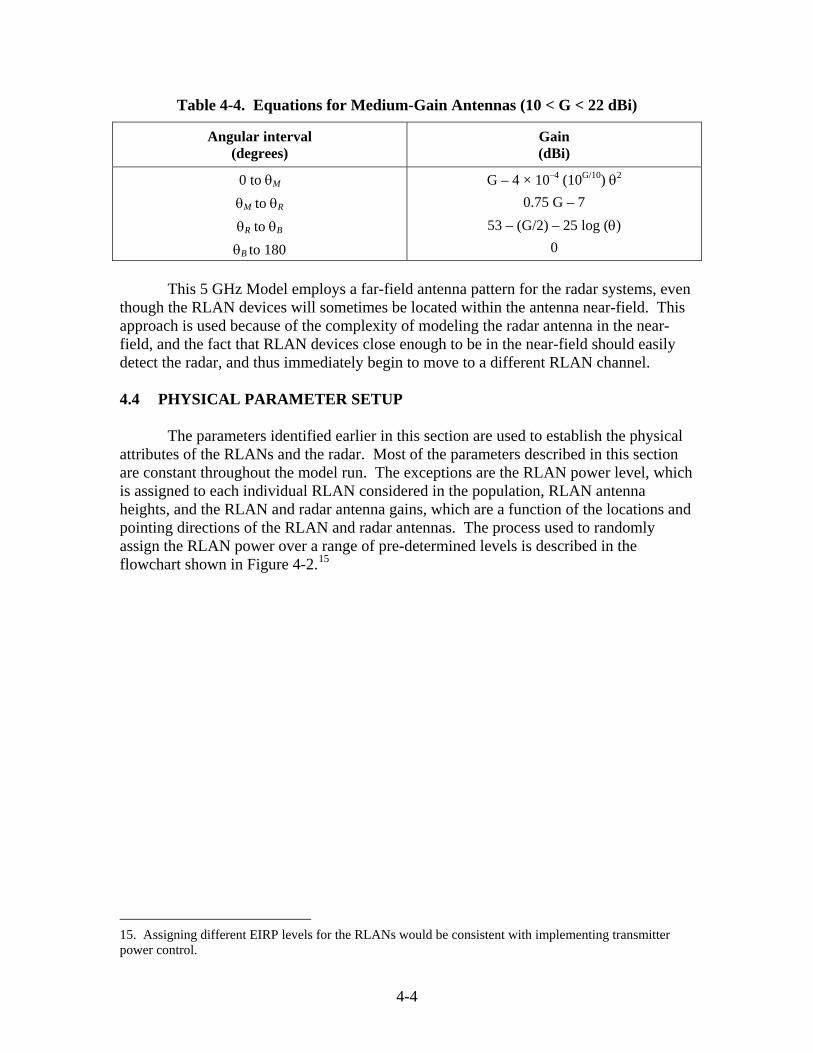
Table 4-4. Equations for Medium-Gain Antennas (10 < G < 22 dBi)


Gain (dBi)

0 to θM

θM to θR

θR to θB

θB to 180

G – 4 × 10–4 (10G/10) θ2

0.75 G – 7 53 – (G/2) – 25 log (θ)

0 This 5 GHz Model employs a far-field antenna pattern for the radar systems, even

though the RLAN devices will sometimes be located within the antenna near-field. This approach is used because of the complexity of modeling the radar antenna in the near-field, and the fact that RLAN devices close enough to be in the near-field should easily detect the radar, and thus immediately begin to move to a different RLAN channel.

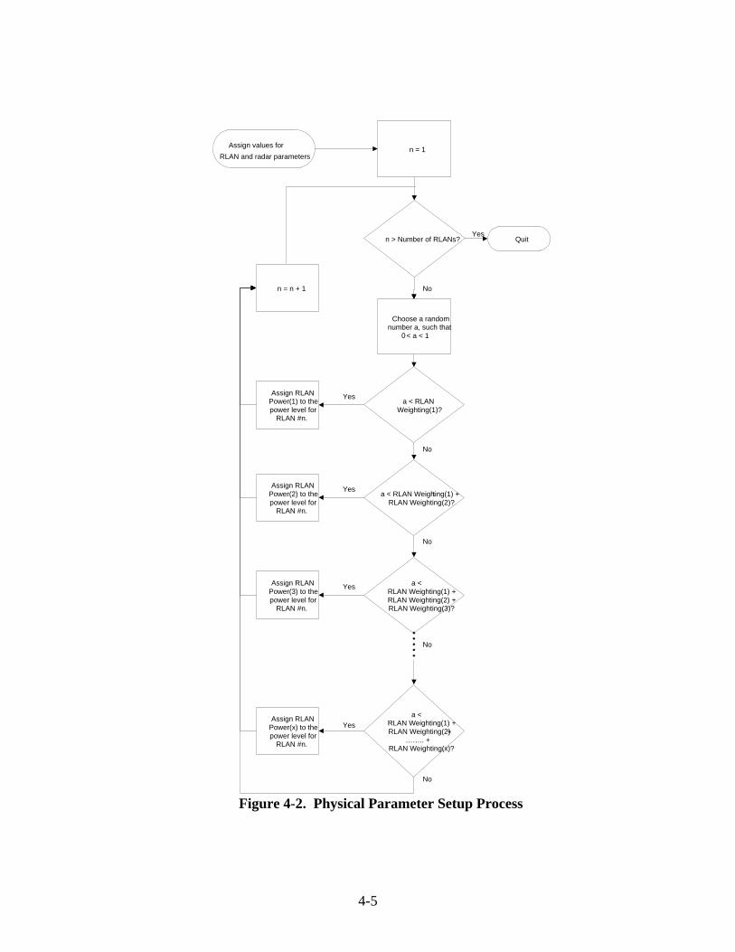
4.4 PHYSICAL PARAMETER SETUP

The parameters identified earlier in this section are used to establish the physical

attributes of the RLANs and the radar. Most of the parameters described in this section are constant throughout the model run. The exceptions are the RLAN power level, which is assigned to each individual RLAN considered in the population, RLAN antenna heights, and the RLAN and radar antenna gains, which are a function of the locations and pointing directions of the RLAN and radar antennas. The process used to randomly assign the RLAN power over a range of pre-determined levels is described in the flowchart shown in Figure 4-2.15

15. Assigning different EIRP levels for the RLANs would be consistent with implementing transmitter power control.

4-4

Assign values forRLAN and radar parameters

n = 1

Choose a randomnumber a, such that

0< a < 1

n > Number of RLANs?

a < RLANWeighting(1)?

Quit

Assign RLANPower(1) to thepower level for

RLAN #n.

a < RLAN Weighting(1) +RLAN Weighting(2)?


RLAN #n.

a <RLAN Weighting(1) +RLAN Weighting(2) +RLAN Weighting(3)?


RLAN #n.

a <RLAN Weighting(1) +RLAN Weighting(2) +

…….. +RLAN Weighting(x)?

Assign RLANPower(x) to thepower level for

RLAN #n.

n = n + 1

Yes

No

Yes

Yes

Yes

Yes

No

No

No

No

Figure 4-2. Physical Parameter Setup Process

4-5

SECTION 5.0 DESCRIPTION OF ANALYSIS MODEL

5.1 INTRODUCTION This section describes the engineering algorithms that the 5 GHz Model uses. The 5 GHz Model uses the methodology described in ITU-R Recommendation M.1461 to compute the received interference power levels at the radar and RLAN receivers.16 A DFS algorithm may provide a means of mitigating this interference by causing the RLAN devices to move to another channel once a radar has been detected on the currently active channel. This model first considers the interference caused by the radar to the RLAN device at the output of the RLAN antenna. If the received interference power level at the output of the RLAN antenna exceeds the DFS detection threshold, the RLAN will cease transmissions and move to another channel. The model then computes the aggregate interference to the radar from the remaining RLAN devices. Each of the technical parameters used in the 5 GHz Model and the radar interference criteria are described in this section. 5.2 ANALYSIS MODEL DESCRIPTION The received interference signal level from the radar at the output of the RLAN antenna is evaluated by using Equation 5-1.

FDRLLLLGGPI LPRLANRadarRLANRadarRadar

RLAN −−−−−++= (5-1) where: IRLAN = Received interference power at the output of the RLAN antenna (dBm); PRadar = Peak power of the radar (dBm);

GRadar = Antenna gain of the radar in the direction (azimuth and elevation) of the RLAN device (dBi); GRLAN = Antenna gain of the RLAN in the direction (azimuth and elevation) of the radar (dBi);

LRadar= Radar transmit insertion loss (dB); LRLAN = RLAN device receiver insertion loss (dB); LP = Propagation loss (dB); LL= Building and non-specific terrain losses (dB); and FDR = Frequency dependent rejection (dB). The antenna gain values GRadar and GRLAN are determined from the appropriate antenna gain patterns. The gain patterns for the model as currently implemented, are considered to be symmetrical relative to boresight (center of mainbeam) in both the 16. International Telecommunication Union-Radiocommunication Sector, Recommendation ITU-R M.1461-1, Procedures for Determining the Potential for Interference Between Radars Operating in the Radiodetermination Service and Systems in Other Services (2000-2003), at Annex 1, (ITU-R M.1461-1) (document available through agency).

5-1

elevation and azimuth plane. Furthermore, the pattern in the elevation plane is considered the same as the azimuth plane. For example, the antenna gain would be the same for X degrees above or below boresight as the gain for X degrees in either the clockwise or counter clockwise direction from boresight. For a given boresight direction of the radar antenna, the 5 GHz Model determines the bearing to the RLAN from the coordinates (azimuth angle) of the radar and RLAN locations. From the difference in the RLAN and radar antenna heights and the distance between the antennas, the model determines the relative elevation angle. These azimuth and elevation angles are then used with the antenna pattern data to determine the appropriate values for GRadar and GRLAN for reach RLAN and radar combination. The 5 GHz Model calculates the received interference signal level using Equation 5-1 for each RLAN device in the distribution. The computed interference signal level is compared to the DFS detection threshold under investigation. If the DFS detection threshold is exceeded for a particular RLAN, the model generates a uniform number and compares it to the probability of an RLAN detecting a radar signal, which in this model is referred to as the probability of coincidence (POC). In the 5 GHz Model bases the POC on a combination of the probability of a radar signal being present and the probability of the DFS detection not being blocked by the DFS-equipped device being in a transmit mode. The POC expresses the probability that the DFS-equipped device is able to detect the radar signal when the radar signal is present. The time the radar signal is present is based on radar parameters such as 3 dB antenna beamwidth, antenna scan rate, pulsewidth, and pulse repetition frequency. The time that the DFS-equipped device is capable of detecting the radar signal is based on the packet length and timing of the RLAN transmissions. The 5 GHz Model uses the parameters and methodology for calculating the POC for the DFS RLAN devices described in Recommendation ITU-R M.1652.17 In implementing the 5 GHz Model, NTIA assumed that the RLAN is capable of detecting power levels in excess of the threshold, and the POC is only considered with respect to investigating the likelihood that radar pulses will occur while the RLAN is in a “quiet period” when DFS detection is possible. If this is the case, the model will move the RLAN to another channel, and the RLAN is not considered (for the remainder of the simulation run) in the calculation of interference to the radar, as given by Equation 5-2.

FDRLLLLGGPI LPRadarRLANRadarRLANRLANRADAR −−−−−++= (5-2)

where: IRADAR = Received interference power at the output of the radar antenna (dBm); PRLAN = Power of the RLAN device (dBm); GRLAN = Antenna gain of the RLAN device in the direction of the radar (dBi); GRadar = Antenna gain of the radar in the direction of the RLAN device (dBi); LRLAN = RLAN device transmit insertion loss (dB); 17. International Telecommunication Union-Radiocommunication Sector, Recommendation ITU-R M.1652, Dynamic Frequency Selection (DFS) in Wireless Access Systems Including Radio Local Area Networks for the Purpose of Protecting the Radiodetermination Service in the 5 GHz Band (2003), at Annex 4 (ITU-R M.1652) (document available through agency).

5-2

LRadar = Radar receiver insertion loss (dB); LP = Propagation loss (dB);

LL= Building and non-specific terrain losses (dB); and FDR = Frequency dependent rejection (dB). The model retains the combination of propagation loss and building/terrain losses that is determined for each IRLAN computation and uses it in the corresponding computation of IRADAR. This is done to maintain reciprocity of the propagation loss over the same path. When the radar antenna is repositioned to initiate a new analysis configuration, a new value for the propagation loss and building/terrain losses is determined for each RLAN and radar combination. Using Equation 5-2, the values are calculated for each RLAN device being considered in the simulation that has not detected a power level from the radar in excess of the DFS detection threshold. These values are then used in the calculation of the aggregate interference to the radar by the remaining RLAN devices using Equation 5-3.

∑=

=N

j

RADARj

AGG II1

(5-3)

where: IAGG = Aggregate interference to the radar from the RLAN devices (Watts); N = Number of RLAN devices remaining in the simulation; and IRADAR = Interference into the radar from an individual RLAN device (Watts). The interference power calculated in Equation 5-2 must be converted from dBm to Watts before calculating the aggregate interference seen by the radar using Equation 5-3. 5.3 DESCRIPTION OF ANALYSIS PARAMETERS The following subsections discuss each of the parameters used in the 5 GHz Model. These parameters include: RLAN and radar technical characteristics such as power and antenna gain, the radiowave propagation models, and frequency dependent rejection.

5.3.1 Radar Peak Power Level (PRadar) The peak power levels of the radars that are used in the 5 GHz Model vary depending on the type (e.g., tracking, scanning) and function (e.g., instrumentation, meteorological) of the radar. The power levels from the radars are given in ITU-R Recommendations M.1461 and M.1313. The peak power levels range from 400 Watts to around 1 million Watts. If additional radars are identified their characteristics can be added to the analysis model.

5-3

5.3.2 Radar Antenna Gain (GRadar) The azimuth and elevation antenna pattern models for the radar are described in Section 4.3.2. The models give the antenna gain as a function of off-axis angle for a given mainbeam antenna gain. The radar mainbeam antenna gains are provided in ITU-R Recommendations M.1461 and M.1313 and range from 30 to 45 dBi. The analysis model includes antenna pattern models for low gain, medium gain, and high gain radar antennas. If additional antenna pattern models are identified in the future, they can be added to the analysis model. 5.3.3 RLAN Power Level (PRLAN) The power levels of the RLAN devices will vary depending on how the individual device is to be deployed. For example, a RLAN in a laptop computer will use lower power than a RLAN device used as an access point. 5.3.4 RLAN Antenna Gain (GRLAN)

The RLAN azimuth and elevation antenna pattern models are described in Section 4.2.3. These antenna patterns can be based on commercially available patterns or ITU-R antenna pattern models. Additional RLAN antenna patterns can be included in the analysis model. 5.3.5 Radar and RLAN Transmitter and Receiver Insertion Losses (LRadar and

LRLAN) The analysis model includes a nominal 2 dB for the insertion losses between the transmitter and receiver antenna and the transmitter and receiver inputs for the radar and the RLAN. 5.3.6 Radiowave Propagation Loss (LP)

The analysis model has three options to compute the radiowave propagation loss

used in the analysis. The propagation option to use depends on the radar type being analyzed. Section 6 contains descriptions of the analysis for each radar type and will indicate the propagation model used. Two options are variations on the freespace propagation model and the other employs an area prediction propagation model. Each of the options available in the model for computing the radiowave propagation loss are described below.

The first option available in the analysis model to compute the radiowave

propagation loss uses the free space equation shown in Equation 5-4.

( ) ( )dLogfLogL FSP 202044.32, ++= (5-4)

5-4

where:

LP, FS = Propagation loss due to free space (dB); f = Frequency (MHz); and d = Distance between transmitter and receiver (km).

Other losses taken into account include the loss due to buildings or non-specific terrain, LL. The total propagation loss is the sum of LP,FS and LL as appropriate. In this option, an average number is chosen to represent a median loss for building blockage, terrain features, multi-path, etc. In this option, the following factor is used. LL = 13 dB

The second option available in the analysis model to compute the radiowave propagation loss uses a variation of Equation 5-4 as shown in Equation 5-5.

( ) ( )dALogfLogL RDP ++= 2044.32, (5-5)

where:

LP, RD = Propagation loss with the distance exponent represented by a uniform random variable (dB); A = A uniform random number between 20 and 35; f = Frequency (MHz); and d = Distance between transmitter and receiver (km).

Other losses taken into account include the loss due to buildings or non-specific terrain, LL. The total propagation loss is the sum of LP,RD and LL as appropriate. In this option, a uniform random number is chosen to represent a varying loss case for building blockage, terrain features, multi-path, etc. Furthermore, it is assumed the following factor applies.

LL = A uniform random value between 0 and 20 dB

The third option available in the analysis model to compute the radiowave propagation loss uses the NTIA Institute for Telecommunication Sciences Irregular Terrain Model (ITM).18 The ITM model computes radiowave propagation based on electromagnetic theory and on statistical analysis of both terrain features and radio measurements to predict the median attenuation as a function of distance and variability of the signal in time and space. A description of the ITM parameters is provided in Table 5-1.

18. National Telecommunications and Information Administration, NTIA Report 82-100, A Guide to the Use of the ITS Irregular Terrain Model in the Area Prediction Mode (1982).

5-5

For each transmit and receive path, the ITM model is used to compute the propagation loss as a function of distance and variability. The ITM model includes three separate aspects of variability: situation variability, location variability, and time variability. For the purpose of simulating instantaneous path loss, ITM should be operated in the single message mode. This mode combines all three types of variability considered in the ITM model into one value. The statistics involved would be described in terms of confidence levels. The parameter values used in the ITM propagation model are provided in Table 5-2. The instantaneous confidence level is simulated by selecting a uniformly generated variability number that is input to the ITM propagation model.

Other losses taken into account include the loss due to buildings or non-specific terrain, LL. The total propagation loss is the sum of LP,RD and LL as appropriate. In this option, a uniform random number is chosen to represent a varying loss for building blockage, terrain features, multi-path, etc. In this option, the following factor is used.

LL = A uniform random value between 0 and 20 dB.

5-6

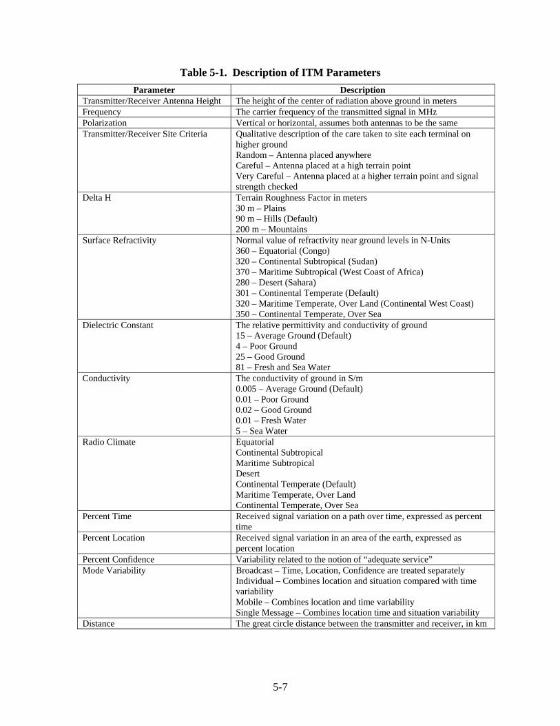
Table 5-1. Description of ITM Parameters Parameter Description

Transmitter/Receiver Antenna Height The height of the center of radiation above ground in meters Frequency The carrier frequency of the transmitted signal in MHz Polarization Vertical or horizontal, assumes both antennas to be the same Transmitter/Receiver Site Criteria Qualitative description of the care taken to site each terminal on

higher ground Random – Antenna placed anywhere Careful – Antenna placed at a high terrain point Very Careful – Antenna placed at a higher terrain point and signal strength checked

Delta H Terrain Roughness Factor in meters 30 m – Plains 90 m – Hills (Default) 200 m – Mountains

Surface Refractivity Normal value of refractivity near ground levels in N-Units 360 – Equatorial (Congo) 320 – Continental Subtropical (Sudan) 370 – Maritime Subtropical (West Coast of Africa) 280 – Desert (Sahara) 301 – Continental Temperate (Default) 320 – Maritime Temperate, Over Land (Continental West Coast) 350 – Continental Temperate, Over Sea

Dielectric Constant The relative permittivity and conductivity of ground 15 – Average Ground (Default) 4 – Poor Ground 25 – Good Ground 81 – Fresh and Sea Water

Conductivity The conductivity of ground in S/m 0.005 – Average Ground (Default) 0.01 – Poor Ground 0.02 – Good Ground 0.01 – Fresh Water 5 – Sea Water

Radio Climate Equatorial Continental Subtropical Maritime Subtropical Desert Continental Temperate (Default) Maritime Temperate, Over Land Continental Temperate, Over Sea

Percent Time Received signal variation on a path over time, expressed as percent time

Percent Location Received signal variation in an area of the earth, expressed as percent location

Percent Confidence Variability related to the notion of “adequate service” Mode Variability Broadcast – Time, Location, Confidence are treated separately

Individual – Combines location and situation compared with time variability Mobile – Combines location and time variability Single Message – Combines location time and situation variability

Distance The great circle distance between the transmitter and receiver, in km

5-7

Table 5-2. ITM Parameter Values Used in the Analysis Model Parameter Description

Transmitter/Receiver Antenna Height

The RLAN antenna height varies depending building deployment and the radar antenna height varies depending on the type of radar

Frequency The mid-band frequency of the radar Polarization Vertical polarization is used for the radar and RLAN Transmitter/Receiver Site Criteria

Random for the RLAN location Careful for the radar location

Delta H 90 meters Surface Refractivity 301 Dielectric Constant 15 Conductivity 0.005 Radio Climate Continental Temperate Percent Time/Location/Variability

1 to 99 percent selected randomly for each RLAN and radar interaction

Mode of Variability Single Message Distance Variable depending on the path under consideration which is

determined by the random placement of the RLAN and radar locations

5.3.7 Frequency Dependent Rejection Frequency Dependent Rejection (FDR) accounts for the fact that not all of the undesired transmitter energy at the receiver input will be available at the detector. FDR is a calculation of the amount of undesired transmitter energy that is rejected by a victim receiver. A detailed description of how to compute FDR can be found in Recommendation ITU-R SM.337-4.19

FDR can be stated mathematically as:

⎥⎥⎥⎥⎥

⎦

⎤

⎢⎢⎢⎢⎢

⎣

⎡

−−

−=

∫

∫∞

∞

0

010

)()(

)(log10

dfffhffp

dfffpFDR

rxtx

tx

(5-6)

where:

txf = Undesired transmitter tuned frequency;

rxf = Victim receiver tuned frequency; )( txffp − = Normalized emission spectrum of the undesired transmitter; )( rxffh − = Normalized transfer function of the victim receiver; and

19. International Telecommunication Union-Radiocommunication Sector, Recommendation ITU-R SM.337-4, Frequency and Distance Separations (1997), at Annex 1 (document available through agency).

5-8

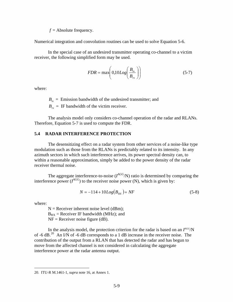
f = Absolute frequency. Numerical integration and convolution routines can be used to solve Equation 5-6. In the special case of an undesired transmitter operating co-channel to a victim receiver, the following simplified form may be used.

⎟⎟⎠

⎞⎜⎜⎝

⎛⎟⎟⎠

⎞⎜⎜⎝

⎛=

rx

tx

BB

LogFDR 10,0max (5-7)

where:

txB = Emission bandwidth of the undesired transmitter; and

rxB = IF bandwidth of the victim receiver. The analysis model only considers co-channel operation of the radar and RLANs. Therefore, Equation 5-7 is used to compute the FDR. 5.4 RADAR INTERFERENCE PROTECTION The desensitizing effect on a radar system from other services of a noise-like type modulation such as those from the RLANs is predictably related to its intensity. In any azimuth sectors in which such interference arrives, its power spectral density can, to within a reasonable approximation, simply be added to the power density of the radar receiver thermal noise. The aggregate interference-to-noise (IAGG/N) ratio is determined by comparing the interference power (IAGG) to the receiver noise power (N), which is given by:

( ) NFBLogN RX ++−= 10 114 (5-8)

where: N = Receiver inherent noise level (dBm); BRX = Receiver IF bandwidth (MHz); and NF = Receiver noise figure (dB). In the analysis model, the protection criterion for the radar is based on an IAGG/N of -6 dB.20 An I/N of -6 dB corresponds to a 1 dB increase in the receiver noise. The contribution of the output from a RLAN that has detected the radar and has begun to move from the affected channel is not considered in calculating the aggregate interference power at the radar antenna output.

20. ITU-R M.1461-1, supra note 16, at Annex 1.

5-9

5.5 INTERFERENCE CALCULATION PROCESS The equations and parameters identified earlier in this section are used to implement the calculation of the aggregate interference to the radar, considering the effect of DFS. The process used in performing these calculations is delineated in the flowchart shown in Figure 5-1.

5-10

Setup allConstants n = 0

n > Number ofRLANs?

n = n + 1 Calculate I RLAN forRLAN #n Calculate I AGG

Quit

IRLAN >Threshold?

Calculate I RADARfor RLAN #n

Rotation Angle = 0

Rotation Angle> Stop Angle?

Rotation Angle =Rotation Angle + 1

Yes

No

No

Yes

No

Remove RLAN #nfrom the

calculationYes

Generate UniformRandom Number

a, such that 0<a<1

a < POC?

Yes

No

Figure 5-1. Interference Calculation Process

5-11

5.6 DFS DETECTION THRESHOLD

The output of the model can be used to determine the impact of the DFS detection threshold on interference to the radar. The DFS detection threshold is the power level (e.g., in dBm) of a signal that will cause the RLAN to cease transmitting and move to another channel. The DFS detection threshold is a key parameter in the success of a RLAN employing DFS. If the detection threshold is too low, the DFS-equipped device could react to noise or other RLAN signals (e.g., packet collisions) which would impact RLAN performance. If the detection threshold is too high, the DFS equipped RLAN could miss detecting the radar signals resulting in potential interference to the radar (e.g., not shifting frequency as intended). Compounding this problem is the lack of beforehand knowledge of the RLAN environment or the radar characteristics.

The impact of the DFS detection threshold was examined by establishing a number of RLAN environments and a number of radar types and deployments. The model was used to perform numerous calculations for various environmental conditions such as: number of RLANs, random RLAN location, random RLAN EIRP level, random RLAN antenna height, radar location, and radar type. The model was then executed hundreds of times to examine the impact of the DFS detection threshold on the IAGG/N. Because of the random selection of many of the analysis parameters, it is a form of Monte Carlo simulation.21 For each series of analysis runs, the model produced distributions of the aggregate interference-to-noise levels as the radar scanned the environment. The model can use various DFS detection thresholds. The radar types and the associated scanning procedures are discussed in Section 6. The output data generated by the model was examined statistically to evaluate the trade-off between the DFS detection threshold and interference to the radar. The results of the model can be used to arrive at a DFS detection threshold that results in an IAGG/N of less than -6 dB.

21. Monte Carlo methods are a class of computational algorithms that rely on repeated random sampling to compute their results. Monte Carlo methods are often used when simulating physical and mathematical systems. Because of their reliance on repeated computation and random or pseudo-random numbers, Monte Carlo methods are most suited to calculation by a computer. Monte Carlo methods tend to be used when it is infeasible or impossible to compute an exact result with a deterministic algorithm.

5-12

http://en.wikipedia.org/wiki/Computation

http://en.wikipedia.org/wiki/Algorithm

http://en.wikipedia.org/wiki/Random

http://en.wikipedia.org/wiki/Computer_simulation

http://en.wikipedia.org/wiki/Physics

http://en.wikipedia.org/wiki/Mathematics

http://en.wikipedia.org/wiki/Random_number

http://en.wikipedia.org/wiki/Pseudorandomness

http://en.wikipedia.org/wiki/Computer

http://en.wikipedia.org/wiki/Deterministic_algorithm

SECTION 6.0 RADAR SPECIFIC MODELING PARAMETERS

6.1 INTRODUCTION In Section 3, the radar deployments considered in the sharing scenarios are described for the various types of radars. This section describes the approach used for each different type of radar evaluated using the 5 GHz Model. 6.2 GROUND-BASED SCANNING RADARS The 5 GHz Model considers ground-based scanning radars by distributing RLAN device locations randomly within the three zones of concentric circles described in Section 3.2 and by placing the radar in a random location within the urban, suburban, or rural zones of concentric circles. The model then begins calculating IRLAN for each RLAN device, assuming the main beam of the radar antenna is pointing at 0 degrees (due east). Either propagation model option 2 or 3 is used in the analysis.22 The model then proceeds to compare each individual value of IRLAN to the DFS detection threshold. In addition to exceeding the DFS detection threshold, the probability of the RLAN detecting the radar signal based on the radar signal parameters (e.g., 3 dB beamwidth, antenna scan rate, pulsewidth, and pulse repetition frequency) and the packet lengths of the RLAN transmissions are also considered. For scanning radars, the POC is determined using the parameters and methodology described in ITU-R Recommendation M.1652.23 For each IRLAN that exceeds the DFS detection threshold, the corresponding RLAN device is eliminated from further consideration during the particular model run. IRADAR is then calculated for each RLAN device remaining in the simulation, and is then used to calculate IAGG. The radar pointing angle is then incremented by one degree in azimuth and the calculations are repeated. This process is continued until two revolutions of the radar antenna are completed, and 720 values of IAGG have been calculated. These values are then used to calculate the IAGG/N ratio as a function of radar rotation angle in degrees.

6.3 GROUND-BASED TRACKING RADARS The 5 GHz Model considers ground-based tracking radars by distributing RLAN device locations randomly within the three zones of concentric circles described in Section 3.2, and by placing the radar along a straight line starting at the urban zone and extending to the end of the rural zone in user defined distance locations.24 The model run then begins by placing the radar at one of the user-defined distance locations. At each of 22. ITU-R M.1652, supra note 17, at Annex 6. 23. Id. at Annex 4. 24. Since the RLAN devices are distributed uniformly within the three zones defining the urban, suburban, and rural areas, the actual location of the tracking radar is not believed to be a critical parameter in the analysis provided that a sufficient number of radar locations and starting azimuths are considered.

6-1

the locations, the model then chooses one of five starting azimuths: 0, 45, 90, 135, or 180 degrees. For each starting azimuth, the model then begins calculating IRLAN for each RLAN device, assuming the main beam of the radar antenna is pointing at 0 degrees elevation in the direction of the starting azimuth. Either propagation model option 2 or 3 is used in the analysis.25 The model then proceeds to compare each individual value of IRLAN to the DFS detection threshold. For each IRLAN that exceeds the DFS detection threshold, the corresponding RLAN device is eliminated from further consideration during the particular model run. The POC for tracking radars is determined using the parameters and methodology described in ITU-R Recommendation M.1652.26 IRADAR is then calculated for each RLAN device remaining in the simulation, and is then used to calculate IAGG. The radar elevation angle is then incremented by one degree and the calculations are repeated. This process is continued until the main beam of the radar antenna is pointing directly at the zenith (elevation angle of 90 degrees). The model then continues the calculations by decrementing the elevation angle one degree at a time. In that way, this process provides simulation of the radar’s tracking of a target from horizon-to-horizon, passing directly overhead. These aggregate values are then used to calculate the IAGG/N ratio as a function of radar rotation angle in degrees.

6.4 SHIP-BASED RADARS The 5 GHz Model considers ship-based scanning radars by distributing RLAN device locations randomly within the three zones of concentric circles described in Section 3.2, and by placing the radar on a course directed at the center of the urban region. The ship is placed at a user-defined initial starting distance away from the center of the urban zone, on a 45 degrees east of north heading. The model then begins calculating IRLAN for each RLAN device, assuming the main beam of the radar antenna is pointing at 0 degrees (due east). The model then proceeds to compare each individual value of IRLAN to the DFS detection threshold. For each IRLAN that exceeds the DFS detection threshold the corresponding RLAN device is eliminated from further consideration during the particular model run. IRADAR is then calculated for each RLAN device remaining in the simulation, and is then used to calculate IAGG. The radar pointing angle is then incremented by one degree and the calculations are repeated. This process is continued until two revolutions of the radar antenna are completed, and 720 values of IAGG have been calculated. The ship is then moved closer to the city in user defined distance increments and the values of IRLAN, IRADAR, and IAGG are calculated again. The maximum aggregate value from each location is then used to calculate the IAGG/N ratio as a function of the distance from the center of the urban region defining the RLAN device distribution.

25. ITU-R M.1652, supra note 17, at Annex 6. 26. Id. at Annex 4.

6-2

6.5 AIRBORNE RADARS Since interference in the mainbeam is the primary concern for the airborne scanning and fixed forward-looking radars, the 5 GHz Model handles them as fixed forward looking, with the main beam of the antenna at an appropriate down-look angle. The radar is placed on a course directed at the center of the urban region, at a user-defined initial starting distance away from the center of the urban zone, on a 45 degrees east of north heading. The model then begins calculating IRLAN for each RLAN device, assuming the main beam of the radar antenna is pointing at 45 degrees (directly toward the city) and at an appropriate down-look angle. The model then proceeds to compare each individual value of IRLAN to the DFS detection threshold. For each IRLAN that exceeds the DFS detection threshold, the corresponding RLAN device is eliminated from further consideration during the particular model run. IRADAR is then calculated for each RLAN device remaining in the simulation, and is then used to calculate IAGG. The radar is then moved closer in specified user defined distance increments toward the center of the urban area and the calculations are repeated. This process is continued until the aircraft reaches the center of the urban area and all values of IAGG have been calculated. The maximum aggregate value from each location is then used to calculate the IAGG/N ratio as a function of the distance from the center of the urban region defining the RLAN device distribution.

6-3

SECTION 7.0 SUMMARY

NTIA developed the 5 GHz Model described in this document to assess the potential aggregate interference from RLANs using DFS to radar systems operating in the 5 GHz frequency range. The model can be used to examine the trade-offs between the detection threshold of the DFS mechanism and the resulting interference to the radar system. The various analytical modules (e.g., propagation models, antenna models) can be modified or new models added to satisfy the requirements of another analysis. In the 5 GHz Model NTIA selected certain parameter values from probability distributions. The range of the distributions and the characterization of the specific random processes can be modified or new ones added as necessary. The MATLAB code for the 5 GHz Model is provided in Appendix A.27 This technical memorandum documents the analysis methodology that NTIA developed and used in assessing interference from RLANs to 5 GHz radar systems. NTIA will consider the analysis methodology and scenarios described in this technical memorandum as it develops the Best Practices Handbook.

27. MATLAB is a numerical computing engineering and programming language.

7-1

APPENDIX A MATLAB CODE FOR 5 GHz MODEL

A.1 INTRODUCTION NTIA considered four types of radar in developing the 5 GHz Model: ground-based scanning radars, ground-based tracking radars, airborne radars, and shipborne radars. The 5 GHz Model consists of four sub-models, which are differentiated according to motion of antenna and antenna pointing. If antenna moves, it is referred to as “mobile;” otherwise it is referred to as “fixed.” If antenna pointing scans, it is referred to as “scan.” If the antenna tracks, it is referred to as “track.” If antenna pointing is not specified, it is fixed pointed. Thus, the four sub-models that make up the 5 GHz Model are referred to as “fixedscan,” “fixedtrack,” “mobilescan,” and “mobile”. The 5 GHz Model consists of 36 MATLAB module files (*.m). Three of these files are devoted for “fixedscan,” three for “fixedtrack,” three for “mobilescan,” and three to “mobile.” The remaining module files are common. In addition there is one *.mat file for each model which saves the radio local area network (RLAN) distribution, including: x, y, z values and associated position vectors, and the region, power, and threshold associated with each RLAN. There is one additional *.mat file which contains the technical characteristics for the nineteen 5 GHz radars described in International Telecommunication Union-Radiocommunication Sector (ITU-R) recommendations.1

The 5 GHz Model works with MATLAB versions 2006 and 2007, including the Mapping Toolbox. The only other necessary file is the pmitm6, which contains the library file for the Irregular Terrain Model.2

A.2 MODEL OVERVIEW Table A-1 lists the file names for the different modules and a brief description of each module.

Table A-1. Module Name Description

pmitm6.dll A program library file for the Irregular Terrain Model. Fixedscan_rlan.mat In this mode the radar is fixed and its antenna scans any number of degrees in azimuth. The

antenna elevation is constant throughout the simulation with the horizontal defined as 0 degrees (elevation angles above the horizontal are positive). In the current version the RLANs are all fixed and their antenna azimuths and elevations remain constant.

fixedtrack_rlan.mat In this mode the radar is fixed and its antenna tracks up to 180 degrees in elevation. The antenna azimuth is constant throughout the simulation with north defined as 0 degrees (the

1. International Telecommunication Union-Radiocommunication Sector, Recommendation ITU-R M.1638, Characteristics of and Protection Criteria for Radiolocation, Aeronautical Radionavigation and Meteorological Radars Operating in the Frequency Bands Between 5250 and 5850 MHz (2003) (document available through agency) and International Telecommunication Union-Radiocommunication Sector, Recommendation ITU-R M.1313-1, Technical Characteristics of Maritime Radionavigation Radars (2000) (document available through agency). 2. The pmitm6.dll file is available from the NTIA Spectrum Engineering and Analysis Division upon request. The pmitm6.dll file should be copied to the “\WINDOWS\SYSTEM\” directory.

A-1

clockwise direction is positive). In the current version the RLANs are all fixed and their antenna azimuths and elevations remain constant.

mobile_rlan.mat In this mode the radar moves north along its current longitude, while its antenna scans any number of degrees in azimuth. If the radar passes through the north pole it will continue along the same great circle path moving south, and its antenna azimuth will flip 180 degrees. The antenna elevation is constant throughout the simulation with the horizontal defined as 0 degrees (elevation angles above the horizontal are positive). In the current version the RLANs are all fixed and their antenna azimuths and elevations remain constant.

mobilescan_rlan.mat In this mode the radar moves north along its current longitude. The antenna azimuth is constant throughout the simulation with north defined as 0 degrees (the clockwise direction is positive). The antenna elevation is also constant throughout the simulation with the horizontal defined as 0 degrees (elevation angles above the horizontal are positive). If the radar passes through the north pole it will continue along the same great circle path moving south, and its antenna azimuth will flip 180 degrees. In the current version the RLANs are all fixed and their antenna azimuths and elevations remain constant.

radar_data.mat Contains technical parameters for 19 different radars in the 5 GHz frequency range from ITU-R Recommendation M.1638.

azelR2ecef.m Converts from local azimuth, elevation, and range, to earth centered earth fixed (ecef) x,y,z coordinates. All angles are radians, including local latitude and longitude. This function is used exclusively to identify the end of an antenna pointing vector. Line 1 h is height above mean sea level. More precisely, it is the height above the reference ellipsoid, as measured along a normal to the ellipsoid. Line 6 Converts azimuth (relative to north) to local vertical (lv) theta, relative to x+, which points east. Line 8 Converts lv coordinates from spherical to x,y,z Line 9 Converts lv to ecef x,y,z. Output is a position vector. Vectors are used to make use of MATLAB dot product, etc. lv2ecef is part of the Mapping Toolbox.

CreateLabelIdentifiers.m This module generates the various labels used in output plots. do_DFS.m Performs the dynamic frequency selection (DFS)

Line 1 I_rlan is a vector containing radar power into each RLAN (in dBm). omega is the current omega vector. POC is the probability of coincidence, which is the probability that the radar will be on between bursts of a given RLAN over the length of time between numsteps. In most cases, the longer the time between numsteps, the higher POC should be if it is to be realistic. new_omega is the omega vector after DFS has been applied. Line 3 new_omega is initialized in case the “for” loop doesn’t change its value. This would correspond to turning every single RLAN “off”.

FDR.m Calculates Frequency Dependent Rejection Line 1 Btx is bandwidth of interfering signal. Brx is bandwidth of victim receiver. Line 2 Currently performs only OTR.

fixedscan_do.m All the *_do files for each submodel are very similar to each other. They perform the heart of the simulations. Line 1 ItIndex is useful when doing more than one iteration. Az is radar antenna pointing azimuth (in radians) at the start of the simulation. El is radar antenna pointing elevation (in radians) at the start of the simulation. Line 2 rlan is the array of structures for the RLANs. YMagOmega keeps track of length of omega across all numsteps. B_RLAN, LT_RLAN, and LR_RLAN are bandwidth, and transmit and receive line losses of RLANs. These parameters are not included in RLAN array of structures to save memory space, since they are the same for all RLANs. numsteps is the abscissa for ItoN and Omega plots. Animate allows radar antenna pointing to be animated. This provides a visual interface into the operation of the model. Line 3 Radar is the radar structure. Gradar_b keeps track of radar gain in the direction of RLAN. gNiterations specifies how many I/N curves to calculate for given simulation. If POC < 1 the different curves should vary from one another to some extent.. Line 4 Omega is the indices of all “on” RLANs. All RLANs are turned “on” at the start of the simulation. Line 5 radar receive noise is calculated here, in watts. Line 6 Initializes YMagOmega to 0. Initializes Iradar, which is aggregate interference from rlans into radar (in watts). If DFS turns all RLANs off, the current iteration will abruptly stop, and the ItoN and Omega plots will show -50 dB and 0 for all remaining numsteps. -50 dB is arbitrary and can be modified by changing the exponent on “1.000e-5”. Line 7 The Omega plot only plots one iteration. In the event the user specifies more than one iteration, it will plot the last one. Line 8 VecLen is magnitude (meters) of radar antenna pointing vector. The value is important only when animating, and is user adjusted for aesthetics. If antenna pointing is below horizontal, you would probably want to reduce the vector length if it would intersect with earth surface. Line 9 If animating, only the last iteration will be animated. Line 11 The end of the radar antenna pointing vector is saved for use in animation. Az is

A-2

current antenna azimuth, always referenced to north, regardless of antenna velocity. El is current antenna elevation, always referenced to the horizontal. Positive radians are above the horizontal. radar.lat and radar.lon are current geodetic coordinates of the radar, and radar.h is the current height above mean sea level. Line 12 Sets the erase mode for animation to ‘xor’, which redraws the plot updating only the antenna pointing vector. If it was set to ‘background’ it would update the pointing vector and redraw all but lines in the path of the pointing vector. Line 15 Gradar_b and Irlan include indices for all RLANs, whether RLANs are “on” or “off”. daz is the azimuthal component of RLAN off-axis angle between antenna main beam and radar. It is set to an arbitrarily low number because RLAN antennas are currently considered to be omnidirectional in azimuth, and the RLAN antenna pattern chooses the larger of azimuth and elevation off-axis components. Since RLAN antennas are considered to be pointing horizontal, the RLAN gain will be a function only of the elevation from RLAN to radar. Line 16 The “for” loop immediately following is where propagation loss is calculated. Therefore, if ITM is chosen, load the “pmitm6.dll” dynamic link library Line 17 This “for” loop establishes vector relationships between RLANs and radar. For this simulation, in which both radar and RLANs are “fixed”, it loops through all RLANs. If any antennas have non-zero velocity, the loop would only consider RLANs which are turned “on”, hence the reference to omega(j) in each line of the loop. Line 18 Rlan2radar is the vector from RLAN pointing to the radar. radar.Pos and rlan.Pos are ecef position vectors. Line 19 The magnitude of previous vector is the slant range, which is used for fs_model and prop_model path loss. Line 20 Great circle distance is also calculated for use with itm_model path loss. Line 21 The RLAN off-axis angle is calculated here. If the antenna pattern is omni-directional, the off-axis angle in radians will be the elevation angle from RLAN to radar. Line 22 This calculates RLAN gain in the direction of the radar. Line 23 Returns the path loss for a particular RLAN/radar link Line 26 In each *_do script this “for” loop is where the simulation takes place, in which the radar antenna pointing and/or position is changed. If RLANs also changed, it would also take place in this loop. Line 28 In fixedscan_do the azimuth of the antenna is stepped clockwise in one degree increments: Az+deg2rad(i) Line 29 In each *_do script the motion of the antenna can be visually reflected in this “if” statement. Line 34 Calculates the radar antenna pointing vector for use in determining radar off-axis angle Line 35 Loop through all “on” RLANs to find radar off-axis angle to RLAN, and associated gain. Only loop through “on” RLANs to minimize time of program execution Line 36 The Rlan2Radar vector is negated to become Radar2Rlan. Line 37 This particular radar antenna pattern is a function of both azimuth and elevation off-axis components. The off-axis angle calculated in 36 is not broken down into components, so an approximation is made by using this in radar_antenna. Line 39 Calculates radar power into each “on” RLAN. dBm is chosen to match units of the threshold. Square brackets must surround fields of the RLAN array of structures on the right side of the equation. This avoids necessity of using a loop, which may run slower. Line 41 Update the omega vector by testing for threshold crossings. Omega contains indices of “on” RLANs. RLAN indices which do not appear in omega are assumed to be “off”. Line 42 If omega is empty, all RLANs are “off”. RLAN interference to radar is impossible, therefore don’t waste time doing any more calculations. The “break” command exits the current “for” loop. In such cases the program resumes at line 51. Line 43 Calculate interference (I) in watts from each “on” RLAN into the radar. Line 46 sum(I) returns the aggregate interference from all “on” RLANs into the radar, for that numstep, which in this case is the current scanning angle. The aggregate interference from “on” RLANs into radar for each numstep is stored in Iradar. Line 48 For the final iteration this “if” statement ends up keeping track of length of Omega vector for each degree of scanning rotation. Line 51 Iradar is converted to dBW Line 52 The radar receiver noise is converted to dBW Line 53 The aggregate I/N ratio for each numstep is returned from the “fixedscan_do” function call.

fixedscan_main.m All the *_main files contain the main subroutine for the respective submodel, and are very similar to each other. Program execution for each submodel begins in the respective *_main script. Line 5 The Boolean “loadrlan” determines whether a new RLAN distribution is generated, or whether the saved distribution is reused. Line 6 Runs the setup script to initialize various simulation parameters Line 7 Determines that the simulation will account for 360 degrees of radar rotation in azimuth. This number could be increased, but not necessary if probability of coincidence is 100%.

A-3

Line 8 Loads parameters for the selected radar into the “radar” structure. Line 10 Returns user-entered number of iterations. An iteration is defined to be a complete simulation. Thus, if more than one iteration is selected the ItoN vs. numsteps plot will show more than one curve. If randomness in one or more variables is permitted from simulation to simulation, these curves will differ at least slightly. Line 11 The starting azimuth for radar antenna pointing must be in radians. Line 12 The starting elevation for radar antenna pointing must be in radians. Line 13 gFinalMatrix contains the radar I/N for each iteration. Line 18 Any time the user elects to generate a new RLAN distribution, it is saved Line 20 If the simulation includes use of high gain RLAN antennas, this line generates an antenna azimuth and elevation for each selected RLAN. In this particular case 10% of RLANs are randomly selected to have directional antennas where their azimuth is randomly selected between 0 and 2pi, and their elevation angle is randomly selected between -10 and 50 degrees.Line 23 A new ItoN vector is generated for each iteration. Each element of ItoN contains an I/N calculation in dB for each degree of radar scanning in azimuth. Line 34 Optionally generate an Excel file containing the Gradar_b matrix.

fixedscan_setup.m All the *_setup files for each submodel are very similar to each other. They allow user to set variables used for the simulation. Line 11 gHighGain provides for the possibility of using directional RLAN antennas, whose azimuth could be randomly generated. Line 12 gStart_Az_deg is the local azimuth (in degrees) of the radar antenna at the start of the simulation. Antenna pointing azimuth is always referenced to north, regardless of the possible velocity of the antenna. Line 13 gStart_El_deg is the local elevation (in degrees) of the radar antenna at the start of the simulation. Antenna pointing elevation is always referenced to the horizontal, with positive radians above the horizontal. Line 16 x and y values of the radar must be coordinated with flat-earth x and y values of the rlan distribution. Currently, the center of the distribution is x=RURAL_RADIUS y=RURAL_RADIUS. All distances are meters unless otherwise noted. Line 24 B_RLAN is the bandwidth of the RLAN (MHz). Since all RLANs are currently assumed to have the same bandwidth this parameter is separated from the RLAN array of structures, to save memory space. Line 25 LR_RLAN is the line loss (dB) for the RLAN receiver. Line 26 LT_RLAN is the line loss for the RLAN transmitter. Line 30 NUM_RLANS is the number of RLANs in the distribution. If loadrlan was set to 1, NUM_RLANS will be ignored. Line 31 RADAR_VALUE is the sequential number used to identify the radar as listed in Rec. ITU_R M.1638 Table 2. The integers 1,2 3, … are used to identify Radar A, B, C, … There are 19 radars to choose from. Line 32 PROP_VALUE identifies which propagation model to use. Line 33 DFSThresh contains the DFS threshold(s) (dBm). Although any number of thresholds could be entered, there should be a one-to-one correspondence between elements of DFSThresh and powers and weights (the next 2 line items). Line 36 This is where POC (the probability of coincidence) is set. Line 37 Re is earth radius at the equator (meters). More precisely, it is the semi-major axis of the earth. Line 38 ellips describes the specified ellipsoid where Re is the semi-major axis and 0 is the eccentricity. The model currently specifies a spherical earth. For the WGS84 ellipsoidal earth use [Re 0.081819184] Line 39 Animate is a Boolean used to provide animation of radar antenna position and pointing.

fixedtrack_do.m Currently, this submodel tracks by maintaining radar antenna azimuth while advancing elevation. Thus all lines of this script are the same as “fixedscan_do” except the following: Line 28 With numsteps set to 180 the antenna pointing vector steps through 180 degrees of elevation about the radar antenna base. El+deg2rad(i).

fixedtrack_main.m See description for fixedscan_main.m. fixedtrack_setup.m See description for fixedscan_main.m. fs_model.m Calculates free space path loss.

Line 4 Frequency (radar.f) must be in MHz. Distance (dist_km) is slant range and must be in kilometers. Line 5 This path loss model is actually 13 dB higher than free-space, but can be readily edited in this script.

get_angle.m Calculates the angle in radians between two vectors. Vectors could be 2 or 3 dimensional. get_gcd.m Calculates the great circle distance between two position vectors get_off_ax.m RLAN off-axis angle is either the elevation from RLAN to radar (for cases where the antenna

pattern is omni-directional in azimuth), or it is the angle between RLAN antenna pointing and the RLAN to radar vector (for high gain antennas). Line 3 Even though gHighGain is true, only a portion of RLAN antennas may be high gain.

A-4

get_pathloss.m All three path loss models require a distance input in kilometers. Line 6 prop_model uses slant range. X.R_b/1000 converts to kilometers. Line 8 itm_model uses great circle distance. Line 10 fs_model uses slant range.

get_radar.m Loads data for appropriate radar. Line 20 Calculates theta, the CCW angle at topocentric origin from x+ to the radar. Also calculates “a”, the distance from origin to radar. Line 21 Converts the initial radar position from local vertical flat earth to ecef spherical earth. Theta flat earth is theta spherical. “a” flat earth becomes the great circle distance on spherical earth. Line 22 Calculates radar latitude and longitude. ecef2geodetic is part of the Mapping Toolbox.

get_rlan_azel.m This function returns a randomly selected azimuth from 0 to 2pi, and a randomly selected elevation from low_el to high_el (radians), for only a portion (weight) of the RLANs of X. The .az and .el fields of other RLANs are assigned to be “empty”.

get_rlan_gain.m This function selects which antenna pattern to use for determining RLAN off=axis gain. get_rlans.m Uses the identical algorithm for determining RLAN distribution used in 5 GHz model. Since that

topology was local vertical flat earth, Lines 80 and 81 of this script also converts to ecef spherical earth.

itm_model.m Calculates ITM path loss. Lines 33 and 36 indicate that randint could be used to generate integer percentages from 1 to 99. randint is contained in the Communications Toolbox. If this is not available, use rand to generate a real number from 0 to 1.

mag.m Calculates the magnitude of a vector. The vector could be 2 or 3 dimensional. mobile_do.m The mobile*_do functions differ from fixed*_do mostly in that the “for” loop that establishes

vector relationships between RLANs and radar must be brought inside of the main simulation loop. This is because in mobile*_do the radar position changes, and thus, so do associated RLAN/radar vectors. Line 16 dist is the great circle distance the radar moves within the simulation. The RLAN distribution is centered about the north pole, and mobile radars always move north along 0° longitude. The “flip” Boolean is required in case dist is great enough to cause the radar to cross 90° latitude. In such cases the radar antenna azimuth will be flipped since the reference north is now facing in the opposite direction. Line 17 track1 calculates a set of numsteps geodetic tracks along a great circle arc equally spaced every dist/(numsteps-1) starting from the current coordinates. These tracks move along 0 azimuth. track1 is part of the Mapping Toolbox. Line 18 This is the “for” loop that contains the simulation. Line 19 Calculates radar ecef position based on next latitude and longitude. Line 21 As radar goes north along 0° longitude, if it crosses the north pole the longitude will no longer be 0°, in which case the radar antenna azimuth needs to be flipped 180°. Line 22 Calculates the end of the radar antenna pointing vector (antenna pointing is fixed in this case, but the radar moves, thus requiring the recalculation). Line 30 This is the RLAN/radar vector relationships “for” loop, which must now be recalculated every numstep, because the radar is moving. Line 37 Radar off-axis angle and antenna gain (Line 38) are added to the “for” loop for efficiency. These values are always (in every *_do function) calculated every numstep by looping through the “on” RLANs.

mobile_main.m Line 7 For the “mobile” submodel, numsteps does not represent the radar antenna pointing azimuth or elevation since these angles are fixed. In this case numsteps represents the distance the radar travels.

mobile_setup.m See description for fixedscan_setup.m. mobilescan_do.m Line 16 In this submodel both antenna velocity and pointing change with time. Therefore the

two must be coordinated with each other. radar.hsr is the horizontal scan rate in degrees per second. numsteps represents the number of degrees of radar antenna scanning, therefore numsteps/radar.hsr is the total time (in seconds) of the scanning. When this is multiplied by the radar speed it gives the distance traveled by the radar during the simulation. Line 17 The radar tracks are determined over a distance “dist” along a 0° azimuth from the starting radar position. Line 22 When calculating the end of the radar antenna pointing vector both antenna pointing and radar location change.

mobilescan_main.m See description for fixedscan_main.m. mobilescan_setup.m gRadarSpeed is the magnitude of radar velocity in meters per second. The direction of radar

velocity always follows along a great circle arc whose beginning azimuth is 0°. Line 40 gRadarSpeed is chosen to be unrealistically fast for demonstration purposes only. If a more realistic speed were chosen the antenna scanning would be so much faster than the forward progress of the radar, that radar position would appear to be stationary.

plotfinalrlans.m Plots the “on” RLAN distribution after DFS has finished turning off potential RLAN interferers. plotItoN.m Plots I/N as a function of angle or distance

A-5

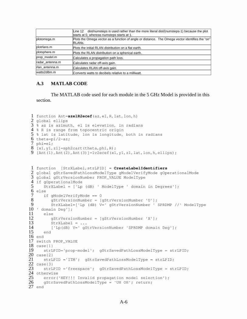
Line 12 dist/numsteps is used rather than the more literal dist/(numsteps-1) because the plot starts at 0, whereas numsteps starts at 1.

plotomega.m Plots the Omega vector as a function of angle or distance. The Omega vector identifies the “on” RLANs.

plotrlans.m Plots the initial RLAN distribution on a flat earth. plotsphere.m Plots the RLAN distribution on a spherical earth. prop_model.m Calculates a propagation path loss. radar_antenna.m Calculates radar off-axis gain. rlan_antenna.m Calculates RLAN off-axis gain. watts2dBm.m Converts watts to decibels relative to a milliwatt.

A.3 MATLAB CODE The MATLAB code used for each module in the 5 GHz Model is provided in this section. function Ant=azelR2ecef(az,el,R,lat,lon,h) 1

2 3 4 5 6 7 8 9

1 2 3 4 5 6 7 8 9

10 11 12 13 14 15 16 17 18 19 20 21 22 23 24 25 26 27

global ellips % az is azimuth, el is elevation, in radians % R is range from topocentric origin % lat is latitude, lon is longitude, both in radians theta=pi/2-az; phi=el; [x1,y1,z1]=sph2cart(theta,phi,R); [Ant(1),Ant(2),Ant(3)]=lv2ecef(x1,y1,z1,lat,lon,h,ellips); function [StrXLabel,strLPID] = CreateLabelIdentifiers global gStrSavedPathLossModelType gModelVerifyMode gOperationalMode global gStrVersionNumber PROP_VALUE ModelType if gOperationalMode StrXLabel = ['Lp (dB) ' ModelType ' domain in Degrees']; else if gModelVerifyMode == 0 gStrVersionNumber = [gStrVersionNumber 'U']; StrXLabel=['Lp (dB) V=' gStrVersionNumber ' SPRDMP //' ModelType ' domain Deg']; else gStrVersionNumber = [gStrVersionNumber 'X']; StrXLabel = ... ['Lp(dB) V=' gStrVersionNumber 'SPRDMP domain Deg']; end end switch PROP_VALUE case{1} strLPID='prop-model'; gStrSavedPathLossModelType = strLPID; case{2} strLPID ='ITM'; gStrSavedPathLossModelType = strLPID; case{3} strLPID ='freespace'; gStrSavedPathLossModelType = strLPID; otherwise error('HEY!!! Invalid propagation model selection'); gStrSavedPathLossModelType = 'UH OH'; return; end

A-6

function new_omega = do_DFS(I_rlan,rlan,omega,poc) 1

2 3 4 5 6 7 8 9

10 11 12 13 14 15

1 2

1 2 3 4 5 6 7 8 9

10 11 12 13 14 15 16 17 18 19 20 21 22 23 24 25 26 27 28 29 30 31 32 33

j=0; new_omega=[]; for i = 1:length(omega) if I_rlan(omega(i)) > rlan(omega(i)).threshold a = rand; if a > poc j = j+1; new_omega(j) = omega(i); end else j = j+1; new_omega(j) = omega(i); end end function [TT] = FDR(Btx,Brx) TT = max(0,10*log10(Btx/Brx)); function ItoN = fixedscan_do(ItIndex,Az,El) global rlan Irlan omega YMagOmega B_RLAN LT_RLAN LR_RLAN PROP_VALUE numsteps Animate global radar Iradar Gradar_b gNiterations POC omega = linspace(1,length(rlan),length(rlan)); k = 1.38e-23; T = 290; B = radar.B*1000000; N = k*T*B; YMagOmega=zeros(1,numsteps);Iradar=ones(1,numsteps)*1.000e-5*N*10^(radar.NF/10); if ItIndex == gNiterations YMagOmega(1) = length(omega); end VecLen=7000; if Animate & ItIndex == gNiterations close(figure(1)); plotsphere; zoom(400); view(0,90); radar.AntTip=azelR2ecef(Az,El,VecLen,radar.lat,radar.lon,radar.h); p=plot3([radar.Pos(1) radar.AntTip(1)],[radar.Pos(2) radar.AntTip(2)],... [radar.Pos(3) radar.AntTip(3)],'g-','EraseMode','xor');%'background' end Gradar_b=zeros(1,length(rlan)); Irlan=zeros(1,length(rlan)); if PROP_VALUE==2 loadlibrary('pmitm6','pmitm6'); end for j = 1:length(omega) rlan(omega(j)).Rlan2Radar=radar.Pos-rlan(omega(j)).Pos; rlan(omega(j)).R_b=mag(rlan(omega(j)).Rlan2Radar); rlan(omega(j)).gcd=get_gcd(radar.Pos,rlan(omega(j)).Pos); rlan(omega(j)).off_ax=get_off_ax(rlan(omega(j))); rlan(omega(j)).G_b=get_rlan_gain(rlan(omega(j))); rlan(omega(j)).Lp_b=get_pathloss(rlan(omega(j))); end if PROP_VALUE==2 unloadlibrary pmitm6; end for i = 1:numsteps radar.AntTip=... azelR2ecef(Az+deg2rad(i),El,VecLen,radar.lat,radar.lon,radar.h); if Animate & ItIndex == gNiterations

A-7

set(p,'xdata',[radar.Pos(1) radar.AntTip(1)],'ydata',... 34 35 36 37 38 39 40 41 42 43 44 45 46 47 48 49 50 51 52 53 54 55 56 57 58 59 60

1 2 3 4 5 6 7 8 9

10 11 12 13 14 15 16 17 18 19 20 21 22 23 24 25 26 27

[radar.Pos(2) radar.AntTip(2)],'zdata',[radar.Pos(3) radar.AntTip(3)]); drawnow end radar.Ant=radar.AntTip-radar.Pos; for j = 1:length(omega) off_ax=get_angle(radar.Ant,-rlan(omega(j)).Rlan2Radar); Gradar_b(omega(j))=radar_antenna(off_ax, radar.G); end Irlan(omega)= watts2dBm(radar.P) - radar.Lt + Gradar_b(omega) - ... [rlan(omega).Lp_b] + [rlan(omega).G_b] - LR_RLAN - FDR(radar.B,B_RLAN); omega = do_DFS(Irlan,rlan,omega,POC); if isempty(omega) break; end I = 0.001*power(10,(watts2dBm([rlan(omega).power]) - LT_RLAN + ... [rlan(omega).G_b] - [rlan(omega).Lp_b] + Gradar_b(omega) - radar.Lr - ... FDR(B_RLAN,radar.B))/10); %watts Iradar(i)=sum(I); if ItIndex == gNiterations if i < numsteps YMagOmega(i+1) = length(omega); end end end Iradar = 10*log10(Iradar); N = 10*log10(N); ItoN = Iradar - N - radar.NF; %fixedscan_main.m global gNiterations gFinalMatrix gStart_Az_deg gStart_El_deg global Irlan Iradar Gradar_b global Animate numsteps gHighGain loadrlan=1; PercentHG=.1; lo_el=-10; hi_el=50; fixedscan_setup; numsteps = 360; get_radar; [gStrXLabel,strLPID] = CreateLabelIdentifiers; gNiterations = input('How many iterations this run??--------------------------->'); start_az_rad = deg2rad(gStart_Az_deg); start_el_rad = deg2rad(gStart_El_deg); gFinalMatrix=ones(numsteps,gNiterations)*-700; % Initial if loadrlan %provides ability to reuse previous rlan distribution load('fixedscan_rlan.mat','rlan'); else get_rlans; save('fixedscan_rlan.mat','rlan'); end if gHighGain rlan=get_rlan_azel(rlan,PercentHG,deg2rad(hi_el),deg2rad(lo_el)); end; for i = 1:gNiterations clear ItoN; ItoN = fixedscan_do(i,start_az_rad,start_el_rad); gFinalMatrix(:,i) = ItoN; end

A-8

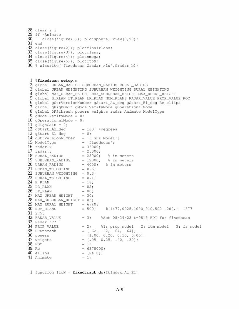
clear i j 28 29 30 31 32 33 34 35 36

1 2 3 4 5 6 7 8 9

10 11 12 13 14 15 16 17 18 19 20 21 22 23 24 25 26 27 28 29 30 31 32 33 34 35 36 37 38 39 40 41

1

if ~Animate close(figure(1)); plotsphere; view(0,90); end close(figure(2)); plotfinalrlans; close(figure(3)); plotrlans; close(figure(4)); plotomega; close(figure(5)); plotItoN; % xlswrite('fixedscan_Gradar.xls',Gradar_b); %fixedscan_setup.m global URBAN_RADIUS SUBURBAN_RADIUS RURAL_RADIUS global URBAN_WEIGHTING SUBURBAN_WEIGHTING RURAL_WEIGHTING global MAX_URBAN_HEIGHT MAX_SUBURBAN_HEIGHT MAX_RURAL_HEIGHT global B_RLAN LT_RLAN LR_RLAN NUM_RLANS RADAR_VALUE PROP_VALUE POC global gStrVersionNumber gStart_Az_deg gStart_El_deg Re ellips global gHighGain gModelVerifyMode gOperationalMode global DFSthresh powers weights radar Animate ModelType gModelVerifyMode = 0; gOperationalMode = 0; gHighGain = 0; gStart_Az_deg = 180; %degrees gStart_El_deg = 0; gStrVersionNumber = '5 GHz Model'; ModelType = 'fixedscan'; radar.x = 36000; radar.y = 25000; RURAL_RADIUS = 25000; % in meters SUBURBAN_RADIUS = 12000; % in meters URBAN_RADIUS = 4000; % in meters URBAN_WEIGHTING = 0.6; SUBURBAN_WEIGHTING = 0.3; RURAL_WEIGHTING = 0.1 ;B_RLAN = 18; LR_RLAN = 02; LT_RLAN = 00; MAX_URBAN_HEIGHT = 30; MAX_SUBURBAN_HEIGHT = 06; MAX_RURAL_HEIGHT = 6;%06 NUM_RLANS = 500; %{1477,0025,1000,010,500 ,200,} 1377 2753 RADAR_VALUE = 3; %Set 08/29/03 t=0815 EDT for fixedscan Radar "C" PROP_VALUE = 2; %1: prop_model 2: itm_model 3: fs_model DFSthresh = [-62, -62, -64, -64]; powers = [1.00, 0.20, 0.10, 0.05]; weights = [.05, 0.25, .40, .30]; POC = 1; Re = 6378000; ellips = [Re 0]; Animate = 1; function ItoN = fixedtrack_do(ItIndex,Az,El)

A-9

2 3 4 5 6 7 8 9

10 11 12 13 14 15 16 17 18 19 20 21 22 23 24 25 26 27 28 29 30 31 32 33 34 35 36 37 38 39 40 41 42 43 44 45 46 47 48 49 50 51 52 53 54 55 56 57 58

global rlan Irlan omega YMagOmega B_RLAN LT_RLAN LR_RLAN PROP_VALUE numsteps Animate global radar Iradar Gradar_b gNiterations POC omega = linspace(1,length(rlan),length(rlan)); k = 1.38e-23; T = 290; B = radar.B*1000000; N = k*T*B; YMagOmega=zeros(1,numsteps); Iradar=ones(1,numsteps)*1.000e-5*N*10^(radar.NF/10); if ItIndex == gNiterations YMagOmega(1) = length(omega); end VecLen=7000; if Animate & ItIndex == gNiterations close(figure(1)); plotsphere; zoom(400); view(0,0); radar.AntTip=azelR2ecef(Az,El,VecLen,radar.lat,radar.lon,radar.h); p=plot3([radar.Pos(1) radar.AntTip(1)],[radar.Pos(2) radar.AntTip(2)],... [radar.Pos(3) radar.AntTip(3)],'g-','EraseMode','xor');%'background' end Gradar_b=zeros(1,length(rlan)); Irlan=zeros(1,length(rlan)); if PROP_VALUE==2 loadlibrary('pmitm6','pmitm6'); end for j = 1:length(omega) rlan(omega(j)).Rlan2Radar=radar.Pos-rlan(omega(j)).Pos; rlan(omega(j)).R_b=mag(rlan(omega(j)).Rlan2Radar); rlan(omega(j)).gcd=get_gcd(radar.Pos,rlan(omega(j)).Pos); rlan(omega(j)).off_ax=get_off_ax(rlan(omega(j))); rlan(omega(j)).G_b=get_rlan_gain(rlan(omega(j))); rlan(omega(j)).Lp_b=get_pathloss(rlan(omega(j))); end if PROP_VALUE==2 unloadlibrary pmitm6; end for i = 1:numsteps radar.AntTip=... azelR2ecef(Az,El+deg2rad(i),VecLen,radar.lat,radar.lon,radar.h); if Animate & ItIndex == gNiterations set(p,'xdata',[radar.Pos(1) radar.AntTip(1)],'ydata',... [radar.Pos(2) radar.AntTip(2)],'zdata',[radar.Pos(3) radar.AntTip(3)]); drawnow end radar.Ant=radar.AntTip-radar.Pos; for j = 1:length(omega) off_ax=get_angle(radar.Ant,-rlan(omega(j)).Rlan2Radar); Gradar_b(omega(j))=radar_antenna(off_ax, radar.G); end Irlan(omega)= watts2dBm(radar.P) - radar.Lt + Gradar_b(omega) - ... [rlan(omega).Lp_b] + [rlan(omega).G_b] - LR_RLAN - FDR(radar.B,B_RLAN); omega = do_DFS(Irlan,rlan,omega,POC); if isempty(omega) break; end I = 0.001*power(10,(watts2dBm([rlan(omega).power]) - LT_RLAN + ... [rlan(omega).G_b] - [rlan(omega).Lp_b] + Gradar_b(omega) - radar.Lr - ... FDR(B_RLAN,radar.B))/10); %watts Iradar(i)=sum(I); if ItIndex == gNiterations if i < numsteps YMagOmega(i+1) = length(omega); end end end Iradar = 10*log10(Iradar);

A-10

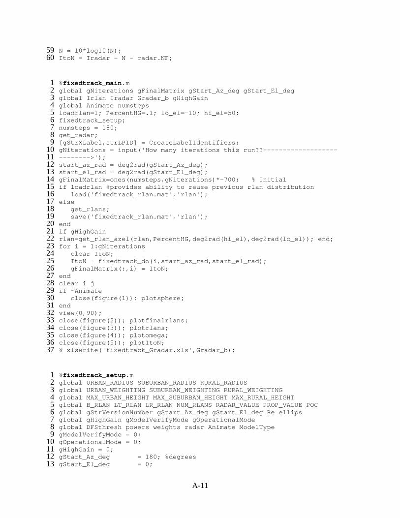
N = 10*log10(N); 59 60

1 2 3 4 5 6 7 8 9

10 11 12 13 14 15 16 17 18 19 20 21 22 23 24 25 26 27 28 29 30 31 32 33 34 35 36 37

1 2 3 4 5 6 7 8 9

10 11 12 13

ItoN = Iradar - N - radar.NF; %fixedtrack_main.m global gNiterations gFinalMatrix gStart_Az_deg gStart_El_deg global Irlan Iradar Gradar_b gHighGain global Animate numsteps loadrlan=1; PercentHG=.1; lo_el=-10; hi_el=50; fixedtrack_setup; numsteps = 180; get_radar; [gStrXLabel,strLPID] = CreateLabelIdentifiers; gNiterations = input('How many iterations this run??--------------------------->'); start_az_rad = deg2rad(gStart_Az_deg); start_el_rad = deg2rad(gStart_El_deg); gFinalMatrix=ones(numsteps,gNiterations)*-700; % Initial if loadrlan %provides ability to reuse previous rlan distribution load('fixedtrack_rlan.mat','rlan'); else get_rlans; save('fixedtrack_rlan.mat','rlan'); end if gHighGain rlan=get_rlan_azel(rlan,PercentHG,deg2rad(hi_el),deg2rad(lo_el)); end; for i = 1:gNiterations clear ItoN; ItoN = fixedtrack_do(i,start_az_rad,start_el_rad); gFinalMatrix(:,i) = ItoN; end clear i j if ~Animate close(figure(1)); plotsphere; end view(0,90); close(figure(2)); plotfinalrlans; close(figure(3)); plotrlans; close(figure(4)); plotomega; close(figure(5)); plotItoN; % xlswrite('fixedtrack_Gradar.xls',Gradar_b); %fixedtrack_setup.m global URBAN_RADIUS SUBURBAN_RADIUS RURAL_RADIUS global URBAN_WEIGHTING SUBURBAN_WEIGHTING RURAL_WEIGHTING global MAX_URBAN_HEIGHT MAX_SUBURBAN_HEIGHT MAX_RURAL_HEIGHT global B_RLAN LT_RLAN LR_RLAN NUM_RLANS RADAR_VALUE PROP_VALUE POC global gStrVersionNumber gStart_Az_deg gStart_El_deg Re ellips global gHighGain gModelVerifyMode gOperationalMode global DFSthresh powers weights radar Animate ModelType gModelVerifyMode = 0; gOperationalMode = 0; gHighGain = 0; gStart_Az_deg = 180; %degrees gStart_El_deg = 0;

A-11

gStrVersionNumber = 'SEAM 1.1'; 14 15 16 17 18 19 20 21 22 23 24 25 26 27 28 29 30 31 32 33 34 35 36 37 38 39 40 41

1 2 3 4 5

1 2

1 2 3

1 2 3 4 5 6 7 8 9

ModelType = 'fixedtrack'; radar.x = 36000; radar.y = 25000; RURAL_RADIUS = 25000; % in meters SUBURBAN_RADIUS = 12000; % in meters URBAN_RADIUS = 4000; % in meters URBAN_WEIGHTING = 0.6; SUBURBAN_WEIGHTING = 0.3; RURAL_WEIGHTING = 0.1; B_RLAN = 18; LR_RLAN = 02; LT_RLAN = 00; MAX_URBAN_HEIGHT = 30; MAX_SUBURBAN_HEIGHT = 06; MAX_RURAL_HEIGHT = 6;%06 NUM_RLANS = 500; %{1477,0025,1000,010,500 ,200,} 1377 2753 RADAR_VALUE = 11; %Set 08/29/03 t=0815 EDT for fixedtrack Radar "K" PROP_VALUE = 2; %1: prop_model 2: itm_model 3: fs_model DFSthresh = [-62, -62, -64, -64]; powers = [1.00, 0.20, 0.10, 0.05]; weights = [.05, 0.25, .40, .30]; POC = 1; Re = 6378000 ;ellips = [Re 0]; Animate = 1; function Lp = fs_model(dist_km) global radar Lprt = 13; Lpfs = 20*log10(radar.f) + 20*log10(dist_km) + 32.44; Lp = Lpfs + Lprt; function theta=get_angle(A,B) theta=acos(dot(A,B)/(mag(A)*mag(B))); function y=get_gcd(xPos,yPos) global Re y=Re*get_angle(xPos,yPos); function ang=get_off_ax(X) global gHighGain ellips if gHighGain & ~isempty(X.az) [lat,lon,h8]=ecef2geodetic(X.Pos(1),X.Pos(2),X.Pos(3),ellips); AntTip=azelR2ecef(X.az,X.el,1000,lat,lon,X.z_a); Ant=AntTip-X.Pos; ang=get_angle(Ant,X.Rlan2Radar); else ang=pi/2-get_angle(X.Rlan2Radar,X.Pos);

A-12

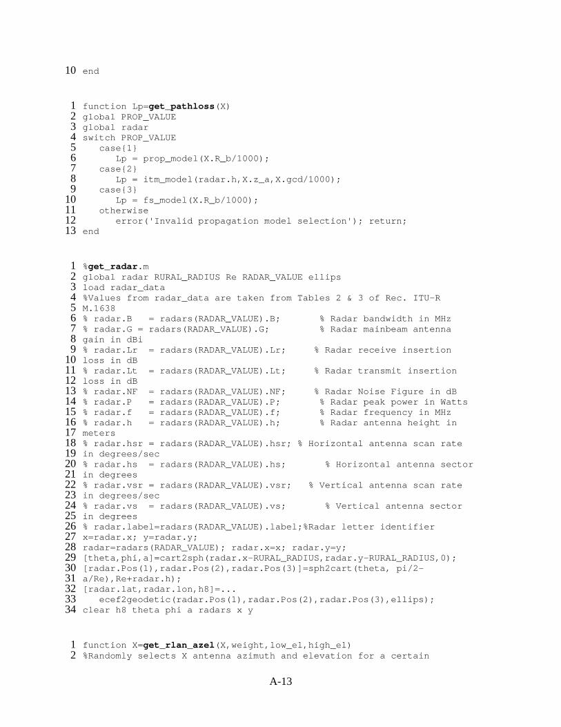
end 10

1 2 3 4 5 6 7 8 9

10 11 12 13

1 2 3 4 5 6 7 8 9

10 11 12 13 14 15 16 17 18 19 20 21 22 23 24 25 26 27 28 29 30 31 32 33 34

1 2

function Lp=get_pathloss(X) global PROP_VALUE global radar switch PROP_VALUE case{1} Lp = prop_model(X.R_b/1000); case{2} Lp = itm_model(radar.h,X.z_a,X.gcd/1000); case{3} Lp = fs_model(X.R_b/1000); otherwise error('Invalid propagation model selection'); return; end %get_radar.m global radar RURAL_RADIUS Re RADAR_VALUE ellips load radar_data %Values from radar_data are taken from Tables 2 & 3 of Rec. ITU-R M.1638 % radar.B = radars(RADAR_VALUE).B; % Radar bandwidth in MHz % radar.G = radars(RADAR_VALUE).G; % Radar mainbeam antenna gain in dBi % radar.Lr = radars(RADAR_VALUE).Lr; % Radar receive insertion loss in dB % radar.Lt = radars(RADAR_VALUE).Lt; % Radar transmit insertion loss in dB % radar.NF = radars(RADAR_VALUE).NF; % Radar Noise Figure in dB % radar.P = radars(RADAR_VALUE).P; % Radar peak power in Watts % radar.f = radars(RADAR_VALUE).f; % Radar frequency in MHz % radar.h = radars(RADAR_VALUE).h; % Radar antenna height in meters % radar.hsr = radars(RADAR_VALUE).hsr; % Horizontal antenna scan rate in degrees/sec % radar.hs = radars(RADAR_VALUE).hs; % Horizontal antenna sector in degrees % radar.vsr = radars(RADAR_VALUE).vsr; % Vertical antenna scan rate in degrees/sec % radar.vs = radars(RADAR_VALUE).vs; % Vertical antenna sector in degrees % radar.label=radars(RADAR_VALUE).label;%Radar letter identifier x=radar.x; y=radar.y; radar=radars(RADAR_VALUE); radar.x=x; radar.y=y; [theta,phi,a]=cart2sph(radar.x-RURAL_RADIUS,radar.y-RURAL_RADIUS,0); [radar.Pos(1),radar.Pos(2),radar.Pos(3)]=sph2cart(theta, pi/2-a/Re),Re+radar.h); [radar.lat,radar.lon,h8]=... ecef2geodetic(radar.Pos(1),radar.Pos(2),radar.Pos(3),ellips); clear h8 theta phi a radars x y function X=get_rlan_azel(X,weight,low_el,high_el) %Randomly selects X antenna azimuth and elevation for a certain

A-13

%percentage of Xs. All angles in radians 3 4 5 6 7 8 9

10 11 12 13

1 2 3 4 5 6 7

1 2 3 4 5 6 7 8 9

10 11 12 13 14 15 16 17 18 19 20 21 22 23 24 25 26 27 28 29 30 31 32 33 34

for i=1:length(X) a=rand; if a<weight X(i).az=2*pi*rand; X(i).el=(high_el-low_el)*rand+low_el; else X(i).az=[]; X(i).el=[]; end end function G=get_rlan_gain(X) global gHighGain if gHighGain & ~isempty(X.az) G=radar_antenna(X.off_ax, 26); else G=rlan_antenna(X.off_ax,X.power); end %get_rlans.m global DFSthresh powers weights rlan NUM_RLANS global URBAN_WEIGHTING SUBURBAN_WEIGHTING RURAL_WEIGHTING global URBAN_RADIUS SUBURBAN_RADIUS RURAL_RADIUS Re global MAX_URBAN_HEIGHT MAX_SUBURBAN_HEIGHT MAX_RURAL_HEIGHT rand('state',sum(100*clock)); for i = 1:NUM_RLANS a = rand; if a >= 0 & a < URBAN_WEIGHTING rlan(i).region = 'urban '; elseif a >= URBAN_WEIGHTING & a < URBAN_WEIGHTING + SUBURBAN_WEIGHTING rlan(i).region = 'suburban'; elseif a >= URBAN_WEIGHTING + SUBURBAN_WEIGHTING & ... a <= URBAN_WEIGHTING + SUBURBAN_WEIGHTING + RURAL_WEIGHTING rlan(i).region = 'rural '; end j = 1; while(j <= length(powers)) a = rand; if a <= sum(weights(1:j)) rlan(i).power = powers(j); rlan(i).threshold = DFSthresh(j); j = length(powers); end j = j+1; end if rlan(i).region == 'urban ' rlan(i).x_a = rand*2*URBAN_RADIUS; rlan(i).y_a = rand*2*URBAN_RADIUS; while rlan(i).y_a > URBAN_RADIUS ... + sqrt(URBAN_RADIUS^2-(rlan(i).x_a-URBAN_RADIUS)^2) |... rlan(i).y_a < URBAN_RADIUS ... - sqrt(URBAN_RADIUS^2-(rlan(i).x_a-URBAN_RADIUS)^2)

A-14

rlan(i).x_a = rand*2*URBAN_RADIUS; 35 36 37 38 39 40 41 42 43 44 45 46 47 48 49 50 51 52 53 54 55 56 57 58 59 60 61 62 63 64 65 66 67 68 69 70 71 72 73 74 75 76 77 78 79 80 81 82 83 84 85 86

1 2

rlan(i).y_a = rand*2*URBAN_RADIUS; end rlan(i).x_a = rlan(i).x_a + RURAL_RADIUS-URBAN_RADIUS; rlan(i).y_a = rlan(i).y_a + RURAL_RADIUS-URBAN_RADIUS; end if rlan(i).region == 'suburban' rlan(i).x_a = rand*2*SUBURBAN_RADIUS; rlan(i).y_a = rand*2*SUBURBAN_RADIUS; while rlan(i).y_a < SUBURBAN_RADIUS - ... sqrt(SUBURBAN_RADIUS^2 - (rlan(i).x_a - SUBURBAN_RADIUS)^2) |... rlan(i).y_a > SUBURBAN_RADIUS + ... sqrt(SUBURBAN_RADIUS^2 - (rlan(i).x_a - SUBURBAN_RADIUS)^2) |... (rlan(i).y_a < SUBURBAN_RADIUS + ... sqrt(URBAN_RADIUS^2 - (rlan(i).x_a - SUBURBAN_RADIUS)^2) &... rlan(i).y_a > SUBURBAN_RADIUS - ... sqrt(URBAN_RADIUS^2 - (rlan(i).x_a - SUBURBAN_RADIUS)^2)) rlan(i).x_a = rand*2*SUBURBAN_RADIUS; rlan(i).y_a = rand*2*SUBURBAN_RADIUS; end rlan(i).x_a = rlan(i).x_a + RURAL_RADIUS-SUBURBAN_RADIUS; rlan(i).y_a = rlan(i).y_a + RURAL_RADIUS-SUBURBAN_RADIUS; end if rlan(i).region == 'rural ' rlan(i).x_a = rand*2*RURAL_RADIUS; rlan(i).y_a = rand*2*RURAL_RADIUS; while rlan(i).y_a < RURAL_RADIUS - ... sqrt(RURAL_RADIUS^2 - (rlan(i).x_a - RURAL_RADIUS)^2) |... rlan(i).y_a > RURAL_RADIUS + ... sqrt(RURAL_RADIUS^2 - (rlan(i).x_a - RURAL_RADIUS)^2) |... (rlan(i).y_a < RURAL_RADIUS + ... sqrt(SUBURBAN_RADIUS^2 - (rlan(i).x_a - RURAL_RADIUS)^2) &... rlan(i).y_a > RURAL_RADIUS - ... sqrt(SUBURBAN_RADIUS^2 - (rlan(i).x_a - RURAL_RADIUS)^2)) rlan(i).x_a = rand*2*RURAL_RADIUS; rlan(i).y_a = rand*2*RURAL_RADIUS; end end if rlan(i).region == 'urban ' rlan(i).z_a = rand*MAX_URBAN_HEIGHT; elseif rlan(i).region == 'suburban' rlan(i).z_a = rand*MAX_SUBURBAN_HEIGHT; elseif rlan(i).region == 'rural ' rlan(i).z_a = rand*MAX_RURAL_HEIGHT; end [theta,phi,a]=cart2sph(rlan(i).x_a-RURAL_RADIUS,rlan(i).y_a-RURAL_RADIUS,0); [rlan(i).Pos(1),rlan(i).Pos(2),rlan(i).Pos(3)]=... sph2cart(theta, pi/2-a/Re,Re+rlan(i).z_a); end function Lp = itm_model(rht_m,tht_m,gcd_km) global radar

A-15

eno_ns_surfref = 301.0; 3 4 5 6 7 8 9

10 11 12 13 14 15 16 17 18 19 20 21 22 23 24 25 26 27 28 29 30 31 32 33 34 35 36 37 38 39 40 41 42 43 44 45 46 47 48 49 50 51 52 53

1 2

sgm_conductivity = 0.005 ;eps_dielect = 15.0; % pol: 0-Horizontal, 1-Vertical % TSiteCriteria, RSiteCriteria: 0 - random, 1 - careful, 2 - very careful % radio_climate: 1-Equatorial, 2-Continental Subtropical, 3-Maritime Tropical, % 4-Desert, 5-Continental Temperate, 6-Maritime Temperate, Over Land, % 7-Maritime Temperate, Over Sea % ModVar: 0 - Single: pctConf is "Time/Situation/Location", pctTime, pctLoc not used % 1 - Individual: pctTime is "Situation/Location", pctConf is "Confidence", % pctLoc not used % 2 - Mobile: pctTime is "Time/Locations (Reliability)", pctConf is % "Confidence", pctLoc not used % 3 - Broadcast: pctTime is "Time", pctLoc is "Location", pctConf is % "Confidence" % pctTime, pctLoc, pctConf: .01 to .99 % errnum: 0- No Error. % 1- Warning: Some parameters are nearly out of range. % Results should be used with caution. % 2- Note: Default parameters have been substituted for impossible ones. % 3- Warning: A combination of parameters is out of range. % Results are probably invalid. % Other- Warning: Some parameters are out of range. % Results are probably invalid. % NOTE: strmode is not used at this time. pol = 1; TSiteCriteria = 0; RSiteCriteria = 2; radio_climate = 5;%4; ModVar = 0; TIME = .5;% randint(1,1,[1,99])/100; pctTime = TIME; LOC = .5; PCON = .5;% randint(1,1,[1,99])/100; DH = 90; AdditionalLoss = 0;%20*rand; if gcd_km < 1 gcd_km = 1.0; end Lp = calllib('pmitm6','ITMAreadBLoss',ModVar, DH, tht_m, rht_m,... gcd_km, TSiteCriteria, RSiteCriteria,... eps_dielect, sgm_conductivity, eno_ns_surfref,... radar.f, radio_climate, pol, pctTime, LOC, PCON) + AdditionalLoss; function y=mag(A) y=sqrt(sum(A.^2));

A-16

function ItoN = mobile_do(ItIndex,Az,El) 1

2 3 4 5 6 7 8 9

10 11 12 13 14 15 16 17 18 19 20 21 22 23 24 25 26 27 28 29 30 31 32 33 34 35 36 37 38 39 40 41 42 43 44 45 46 47 48 49 50 51 52 53 54 55 56

global rlan Irlan omega YMagOmega B_RLAN LT_RLAN LR_RLAN PROP_VALUE numsteps Animate global radar Iradar Gradar_b gNiterations POC radarlat radarlon ellips dist omega = linspace(1,length(rlan),length(rlan)); k = 1.38e-23; T = 290; B = radar.B*1000000; N = k*T*B; YMagOmega=zeros(1,numsteps); Iradar=ones(1,numsteps)*1.000e-5*N*10^(radar.NF/10); if ItIndex == gNiterations YMagOmega(1) = length(omega); end VecLen=5000; if Animate & ItIndex == gNiterations close(figure(1)); plotsphere; zoom(200); view(0,90); radar.AntTip=azelR2ecef(Az,El,VecLen,radar.lat,radar.lon,radar.h); p=plot3([radar.Pos(1) radar.AntTip(1)],[radar.Pos(2) radar.AntTip(2)],... [radar.Pos(3) radar.AntTip(3)],'g-','EraseMode','xor');%'background' end Gradar_b=zeros(1,length(rlan)); Irlan=zeros(1,length(rlan)); dist=radar.x; flip=1; [radarlat,radarlon]=track1(radar.lat,radar.lon,0,dist,ellips,'radians',numsteps); for i = 1:numsteps [radar.Pos(1),radar.Pos(2),radar.Pos(3)]=... geodetic2ecef(radarlat(i),radarlon(i),radar.h,ellips); if flip & radarlon(i)~=0 Az=Az+pi; flip=0; end radar.AntTip=azelR2ecef(Az,El,VecLen,radarlat(i),radarlon(i),radar.h); if Animate & ItIndex == gNiterations set(p,'xdata',[radar.Pos(1) radar.AntTip(1)],'ydata',... [radar.Pos(2) radar.AntTip(2)],'zdata',[radar.Pos(3) radar.AntTip(3)]); drawnow end radar.Ant=radar.AntTip-radar.Pos; if PROP_VALUE==2 loadlibrary('pmitm6','pmitm6'); end for j = 1:length(omega) rlan(omega(j)).Rlan2Radar=radar.Pos-rlan(omega(j)).Pos; rlan(omega(j)).R_b=mag(rlan(omega(j)).Rlan2Radar); rlan(omega(j)).gcd=get_gcd(radar.Pos,rlan(omega(j)).Pos); rlan(omega(j)).off_ax=get_off_ax(rlan(omega(j))); rlan(omega(j)).G_b=get_rlan_gain(rlan(omega(j))); rlan(omega(j)).Lp_b=get_pathloss(rlan(omega(j))); off_ax=get_angle(radar.Ant,-rlan(omega(j)).Rlan2Radar); Gradar_b(omega(j))=radar_antenna(off_ax, radar.G); end if PROP_VALUE==2 unloadlibrary pmitm6; end Irlan(omega)= watts2dBm(radar.P) - radar.Lt + Gradar_b(omega) - ... [rlan(omega).Lp_b] + [rlan(omega).G_b] - LR_RLAN - FDR(radar.B,B_RLAN); omega = do_DFS(Irlan,rlan,omega,POC); if isempty(omega) break; end I = 0.001*power(10,(watts2dBm([rlan(omega).power]) - LT_RLAN + ... [rlan(omega).G_b] - [rlan(omega).Lp_b] + Gradar_b(omega) - radar.Lr - ...

A-17

FDR(B_RLAN,radar.B))/10); %watts 57 58 59 60 61 62 63 64 65

1 2 3 4 5 6 7 8 9

10 11 12 13 14 15 16 17 18 19 20 21 22 23 24 25 26 27 28 29 30 31 32 33 34 35 36 37

1 2 3 4 5 6

Iradar(i)=sum(I); if ItIndex == gNiterations if i < numsteps YMagOmega(i+1) = length(omega); end end end Iradar = 10*log10(Iradar); N = 10*log10(N); ItoN = Iradar - N - radar.NF; %mobile_main.m global gNiterations gFinalMatrix gStart_Az_deg gStart_El_deg global Irlan Iradar Gradar_b global Animate numsteps radarlat radarlon dist gHighGain loadrlan=1; PercentHG=.1; lo_el=-10; hi_el=50; mobile_setup; numsteps = 100; get_radar; [gStrXLabel,strLPID] = CreateLabelIdentifiers; gNiterations = input('How many iterations this run??--------------------------->'); start_az_rad = deg2rad(gStart_Az_deg); start_el_rad = deg2rad(gStart_El_deg); gFinalMatrix=ones(numsteps,gNiterations)*-700; % Initial if loadrlan %provides ability to reuse previous rlan distribution load('mobile_rlan.mat','rlan'); else get_rlans; save('mobile_rlan.mat','rlan'); end if gHighGain rlan=get_rlan_azel(rlan,PercentHG,deg2rad(hi_el),deg2rad(lo_el)); end; for i = 1:gNiterations clear ItoN; ItoN = mobile_do(i,start_az_rad,start_el_rad); gFinalMatrix(:,i) = ItoN; end clear i j if ~Animate close(figure(1)); plotsphere; end view(0,90); close(figure(2)); plotfinalrlans; close(figure(3)); plotrlans; close(figure(4)); plotomega ;close(figure(5)); plotItoN; % xlswrite('mobile_Gradar.xls',Gradar_b); %mobile_setup.m global URBAN_RADIUS SUBURBAN_RADIUS RURAL_RADIUS global URBAN_WEIGHTING SUBURBAN_WEIGHTING RURAL_WEIGHTING global MAX_URBAN_HEIGHT MAX_SUBURBAN_HEIGHT MAX_RURAL_HEIGHT global B_RLAN LT_RLAN LR_RLAN NUM_RLANS RADAR_VALUE PROP_VALUE POC global gStrVersionNumber gStart_Az_deg gStart_El_deg Re ellips

A-18

global gHighGain gModelVerifyMode gOperationalMode 7 8 9

10 11 12 13 14 15 16 17 18 19 20 21 22 23 24 25 26 27 28 29 30 31 32 33 34 35 36 37 38 39 40

1 2 3 4 5 6 7 8 9

10 11 12 13 14 15 16 17 18 19 20

global DFSthresh powers weights radar Animate ModelType gModelVerifyMode = 0; gOperationalMode = 0; gHighGain = 0; gStart_Az_deg = 0; %degrees gStart_El_deg = -50; gStrVersionNumber = '5 GHz Model'; ModelType = 'mobile'; radar.x = 50000;%125000 36000 radar.y = 25000; RURAL_RADIUS = 25000; % in meters SUBURBAN_RADIUS = 12000; % in meters URBAN_RADIUS = 4000; % in meters URBAN_WEIGHTING = 0.6; SUBURBAN_WEIGHTING = 0.3; RURAL_WEIGHTING = 0.1 ;B_RLAN = 18; LR_RLAN = 02; LT_RLAN = 00; MAX_URBAN_HEIGHT = 30; MAX_SUBURBAN_HEIGHT = 06; MAX_RURAL_HEIGHT = 6;%06 NUM_RLANS = 500; %{1477,0025,1000,010,500 ,200,} 1377 2753 RADAR_VALUE = 18; %Airborne Radar 18 or 19 PROP_VALUE = 2; %1: prop_model 2: itm_model 3: fs_model DFSthresh = [-62, -62, -64, -64]; powers = [1.00, 0.20, 0.10, 0.05]; weights = [.05, 0.25, .40, .30]; POC = 1; Re = 6378000; ellips = [Re 0]; Animate = 1; function ItoN = mobilescan_do(ItIndex,Az,El) global rlan Irlan omega YMagOmega B_RLAN LT_RLAN LR_RLAN PROP_VALUE numsteps Animate global radar Iradar Gradar_b gNiterations POC radarlat radarlon ellips gRadarSpeed omega = linspace(1,length(rlan),length(rlan)); k = 1.38e-23; T = 290; B = radar.B*1000000; N = k*T*B; YMagOmega=zeros(1,numsteps); Iradar=ones(1,numsteps)*1.000e-5*N*10^(radar.NF/10); if ItIndex == gNiterations YMagOmega(1) = length(omega); end VecLen=5000; if Animate & ItIndex == gNiterations close(figure(1)); plotsphere; zoom(1000); view(0,90); radar.AntTip=azelR2ecef(Az,El,VecLen,radar.lat,radar.lon,radar.h); p=plot3([radar.Pos(1) radar.AntTip(1)],[radar.Pos(2) radar.AntTip(2)],... [radar.Pos(3) radar.AntTip(3)],'g-','EraseMode','xor');%'background' end Gradar_b=zeros(1,length(rlan)); Irlan=zeros(1,length(rlan));

A-19

dist=numsteps/radar.hsr*gRadarSpeed; flip=1; 21 22 23 24 25 26 27 28 29 30 31 32 33 34 35 36 37 38 39 40 41 42 43 44 45 46 47 48 49 50 51 52 53 54 55 56 57 58 59 60 61 62 63 64 65 66

1 2 3 4 5 6 7 8

[radarlat,radarlon]=track1(radar.lat,radar.lon,0,dist,ellips,'radians',numsteps); for i = 1:numsteps [radar.Pos(1),radar.Pos(2),radar.Pos(3)]=... geodetic2ecef(radarlat(i),radarlon(i),radar.h,ellips); if flip & radarlon(i)~=0 Az=Az+pi; flip=0; end radar.AntTip=azelR2ecef(Az+deg2rad(i),El,VecLen,radarlat(i),radarlon(i),radar.h); if Animate & ItIndex == gNiterations set(p,'xdata',[radar.Pos(1) radar.AntTip(1)],'ydata',... [radar.Pos(2) radar.AntTip(2)],'zdata',[radar.Pos(3) radar.AntTip(3)]); drawnow end radar.Ant=radar.AntTip-radar.Pos; if PROP_VALUE==2 loadlibrary('pmitm6','pmitm6'); end for j = 1:length(omega) rlan(omega(j)).Rlan2Radar=radar.Pos-rlan(omega(j)).Pos; rlan(omega(j)).R_b=mag(rlan(omega(j)).Rlan2Radar); rlan(omega(j)).gcd=get_gcd(radar.Pos,rlan(omega(j)).Pos); rlan(omega(j)).off_ax=get_off_ax(rlan(omega(j))); rlan(omega(j)).G_b=get_rlan_gain(rlan(omega(j))); rlan(omega(j)).Lp_b=get_pathloss(rlan(omega(j))); off_ax=get_angle(radar.Ant,-rlan(omega(j)).Rlan2Radar); Gradar_b(omega(j))=radar_antenna(off_ax, radar.G); end if PROP_VALUE==2 unloadlibrary pmitm6; end Irlan(omega)= watts2dBm(radar.P) - radar.Lt + Gradar_b(omega) - ... [rlan(omega).Lp_b] + [rlan(omega).G_b] - LR_RLAN - FDR(radar.B,B_RLAN); omega = do_DFS(Irlan,rlan,omega,POC); if isempty(omega) break; end I = 0.001*power(10,(watts2dBm([rlan(omega).power]) - LT_RLAN + ... [rlan(omega).G_b] - [rlan(omega).Lp_b] + Gradar_b(omega) - radar.Lr - ... FDR(B_RLAN,radar.B))/10); %watts Iradar(i)=sum(I); if ItIndex == gNiterations if i < numsteps YMagOmega(i+1) = length(omega); end end end Iradar = 10*log10(Iradar); N = 10*log10(N); ItoN = Iradar - N - radar.NF; %mobilescan_main.m global gNiterations gFinalMatrix gStart_Az_deg gStart_El_deg global Irlan Iradar Gradar_b global Animate numsteps radarlat radarlon gHighGain loadrlan=1; PercentHG=.1; lo_el=-10; hi_el=50; mobilescan_setup; numsteps = 180; get_radar;

A-20

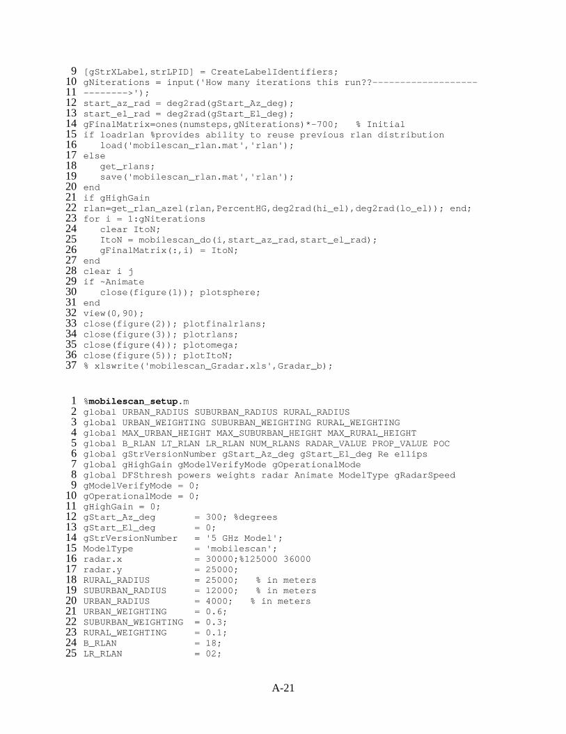
[gStrXLabel,strLPID] = CreateLabelIdentifiers; 9 10 11 12 13 14 15 16 17 18 19 20 21 22 23 24 25 26 27 28 29 30 31 32 33 34 35 36 37

1 2 3 4 5 6 7 8 9

10 11 12 13 14 15 16 17 18 19 20 21 22 23 24 25

gNiterations = input('How many iterations this run??--------------------------->'); start_az_rad = deg2rad(gStart_Az_deg); start_el_rad = deg2rad(gStart_El_deg); gFinalMatrix=ones(numsteps,gNiterations)*-700; % Initial if loadrlan %provides ability to reuse previous rlan distribution load('mobilescan_rlan.mat','rlan'); else get_rlans; save('mobilescan_rlan.mat','rlan'); end if gHighGain rlan=get_rlan_azel(rlan,PercentHG,deg2rad(hi_el),deg2rad(lo_el)); end; for i = 1:gNiterations clear ItoN; ItoN = mobilescan_do(i,start_az_rad,start_el_rad); gFinalMatrix(:,i) = ItoN; end clear i j if ~Animate close(figure(1)); plotsphere; end view(0,90); close(figure(2)); plotfinalrlans; close(figure(3)); plotrlans; close(figure(4)); plotomega; close(figure(5)); plotItoN; % xlswrite('mobilescan_Gradar.xls',Gradar_b); %mobilescan_setup.m global URBAN_RADIUS SUBURBAN_RADIUS RURAL_RADIUS global URBAN_WEIGHTING SUBURBAN_WEIGHTING RURAL_WEIGHTING global MAX_URBAN_HEIGHT MAX_SUBURBAN_HEIGHT MAX_RURAL_HEIGHT global B_RLAN LT_RLAN LR_RLAN NUM_RLANS RADAR_VALUE PROP_VALUE POC global gStrVersionNumber gStart_Az_deg gStart_El_deg Re ellips global gHighGain gModelVerifyMode gOperationalMode global DFSthresh powers weights radar Animate ModelType gRadarSpeed gModelVerifyMode = 0; gOperationalMode = 0; gHighGain = 0; gStart_Az_deg = 300; %degrees gStart_El_deg = 0; gStrVersionNumber = '5 GHz Model'; ModelType = 'mobilescan'; radar.x = 30000;%125000 36000 radar.y = 25000; RURAL_RADIUS = 25000; % in meters SUBURBAN_RADIUS = 12000; % in meters URBAN_RADIUS = 4000; % in meters URBAN_WEIGHTING = 0.6; SUBURBAN_WEIGHTING = 0.3; RURAL_WEIGHTING = 0.1; B_RLAN = 18; LR_RLAN = 02;

A-21

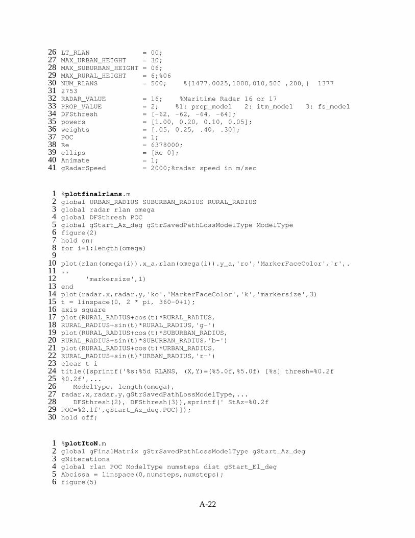
LT_RLAN = 00; 26 27 28 29 30 31 32 33 34 35 36 37 38 39 40 41

1 2 3 4 5 6 7 8 9

10 11 12 13 14 15 16 17 18 19 20 21 22 23 24 25 26 27 28 29 30

1 2 3 4 5 6

MAX_URBAN_HEIGHT = 30; MAX_SUBURBAN_HEIGHT = 06; MAX_RURAL_HEIGHT = 6;%06 NUM_RLANS = 500; %{1477,0025,1000,010,500 ,200,} 1377 2753 RADAR_VALUE = 16; %Maritime Radar 16 or 17 PROP_VALUE = 2; %1: prop_model 2: itm_model 3: fs_model DFSthresh = [-62, -62, -64, -64]; powers = [1.00, 0.20, 0.10, 0.05]; weights = [.05, 0.25, .40, .30]; POC = 1; Re = 6378000; ellips = [Re 0]; Animate = 1; gRadarSpeed = 2000;%radar speed in m/sec %plotfinalrlans.m global URBAN_RADIUS SUBURBAN_RADIUS RURAL_RADIUS global radar rlan omega global DFSthresh POC global gStart_Az_deg gStrSavedPathLossModelType ModelType figure(2) hold on; for i=1:length(omega) plot(rlan(omega(i)).x_a,rlan(omega(i)).y_a,'ro','MarkerFaceColor','r',... 'markersize',1) end plot(radar.x,radar.y,'ko','MarkerFaceColor','k','markersize',3) t = linspace(0, 2 * pi, 360-0+1); axis square plot(RURAL_RADIUS+cos(t)*RURAL_RADIUS, RURAL_RADIUS+sin(t)*RURAL_RADIUS,'g-') plot(RURAL_RADIUS+cos(t)*SUBURBAN_RADIUS, RURAL_RADIUS+sin(t)*SUBURBAN_RADIUS,'b-') plot(RURAL_RADIUS+cos(t)*URBAN_RADIUS, RURAL_RADIUS+sin(t)*URBAN_RADIUS,'r-') clear t i title([sprintf('%s:%5d RLANS, (X,Y)=(%5.0f,%5.0f) [%s] thresh=%0.2f %0.2f',... ModelType, length(omega), radar.x,radar.y,gStrSavedPathLossModelType,... DFSthresh(2), DFSthresh(3)),sprintf(' StAz=%0.2f POC=%2.1f',gStart_Az_deg,POC)]); hold off; %plotItoN.m global gFinalMatrix gStrSavedPathLossModelType gStart_Az_deg gNiterations global rlan POC ModelType numsteps dist gStart_El_deg Abcissa = linspace(0,numsteps,numsteps); figure(5)

A-22

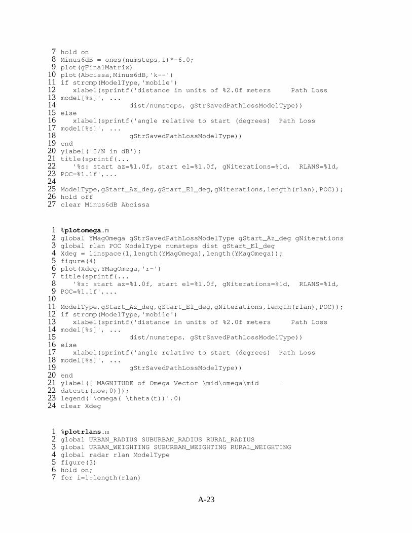
hold on 7 8 9

10 11 12 13 14 15 16 17 18 19 20 21 22 23 24 25 26 27

1 2 3 4 5 6 7 8 9

10 11 12 13 14 15 16 17 18 19 20 21 22 23 24

1 2 3 4 5 6 7

Minus6dB = ones(numsteps,1)*-6.0; plot(gFinalMatrix) plot(Abcissa,Minus6dB,'k--') if strcmp(ModelType,'mobile') xlabel(sprintf('distance in units of %2.0f meters Path Loss model[%s]', ... dist/numsteps, gStrSavedPathLossModelType)) else xlabel(sprintf('angle relative to start (degrees) Path Loss model[%s]', ... gStrSavedPathLossModelType)) end ylabel('I/N in dB'); title(sprintf(... '%s: start az=%1.0f, start el=%1.0f, gNiterations=%1d, RLANS=%1d, POC=%1.1f',... ModelType,gStart_Az_deg,gStart_El_deg,gNiterations,length(rlan),POC)); hold off clear Minus6dB Abcissa %plotomega.m global YMagOmega gStrSavedPathLossModelType gStart_Az_deg gNiterations global rlan POC ModelType numsteps dist gStart_El_deg Xdeg = linspace(1,length(YMagOmega),length(YMagOmega)); figure(4) plot(Xdeg,YMagOmega,'r-') title(sprintf(... '%s: start az=%1.0f, start el=%1.0f, gNiterations=%1d, RLANS=%1d, POC=%1.1f',... ModelType,gStart_Az_deg,gStart_El_deg,gNiterations,length(rlan),POC)); if strcmp(ModelType,'mobile') xlabel(sprintf('distance in units of %2.0f meters Path Loss model[%s]', ... dist/numsteps, gStrSavedPathLossModelType)) else xlabel(sprintf('angle relative to start (degrees) Path Loss model[%s]', ... gStrSavedPathLossModelType)) end ylabel(['MAGNITUDE of Omega Vector \mid\omega\mid ' datestr(now,0)]); legend('\omega( \theta(t))',0) clear Xdeg %plotrlans.m global URBAN_RADIUS SUBURBAN_RADIUS RURAL_RADIUS global URBAN_WEIGHTING SUBURBAN_WEIGHTING RURAL_WEIGHTING global radar rlan ModelType figure(3) hold on; for i=1:length(rlan)

A-23

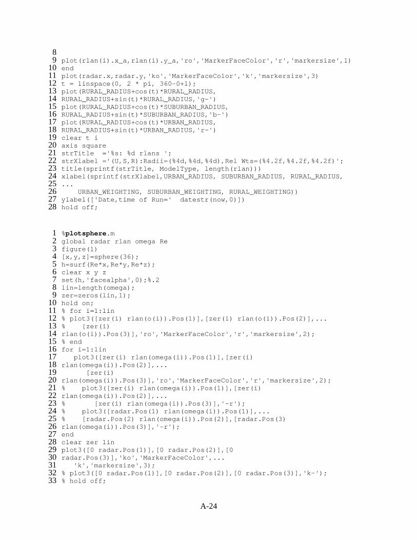
8 9

10 11 12 13 14 15 16 17 18 19 20 21 22 23 24 25 26 27 28

1 2 3 4 5 6 7 8 9

10 11 12 13 14 15 16 17 18 19 20 21 22 23 24 25 26 27 28 29 30 31 32 33

plot(rlan(i).x_a,rlan(i).y_a,'ro','MarkerFaceColor','r','markersize',1) end plot(radar.x,radar.y,'ko','MarkerFaceColor','k','markersize',3) t = linspace(0, 2 * pi, 360-0+1); plot(RURAL_RADIUS+cos(t)*RURAL_RADIUS, RURAL_RADIUS+sin(t)*RURAL_RADIUS,'g-') plot(RURAL_RADIUS+cos(t)*SUBURBAN_RADIUS, RURAL_RADIUS+sin(t)*SUBURBAN_RADIUS,'b-') plot(RURAL_RADIUS+cos(t)*URBAN_RADIUS, RURAL_RADIUS+sin(t)*URBAN_RADIUS,'r-') clear t i axis square strTitle ='%s: %d rlans '; strXlabel ='(U,S,R):Radii=(%4d,%4d,%4d),Rel Wts=(%4.2f,%4.2f,%4.2f)'; title(sprintf(strTitle, ModelType, length(rlan))) xlabel(sprintf(strXlabel,URBAN_RADIUS, SUBURBAN_RADIUS, RURAL_RADIUS, ... URBAN_WEIGHTING, SUBURBAN_WEIGHTING, RURAL_WEIGHTING)) ylabel(['Date,time of Run=' datestr(now,0)]) hold off; %plotsphere.m global radar rlan omega Re figure(1) [x,y,z]=sphere(36); h=surf(Re*x,Re*y,Re*z); clear x y z set(h,'facealpha',0);%.2 lin=length(omega) ;zer=zeros(lin,1); hold on; % for i=1:lin % plot3([zer(i) rlan(o(i)).Pos(1)],[zer(i) rlan(o(i)).Pos(2)],... % [zer(i) rlan(o(i)).Pos(3)],'ro','MarkerFaceColor','r','markersize',2); % end for i=1:lin plot3([zer(i) rlan(omega(i)).Pos(1)],[zer(i) rlan(omega(i)).Pos(2)],... [zer(i) rlan(omega(i)).Pos(3)],'ro','MarkerFaceColor','r','markersize',2); % plot3([zer(i) rlan(omega(i)).Pos(1)],[zer(i) rlan(omega(i)).Pos(2)],... % [zer(i) rlan(omega(i)).Pos(3)],'-r'); % plot3([radar.Pos(1) rlan(omega(i)).Pos(1)],... % [radar.Pos(2) rlan(omega(i)).Pos(2)],[radar.Pos(3) rlan(omega(i)).Pos(3)],'-r'); end clear zer lin plot3([0 radar.Pos(1)],[0 radar.Pos(2)],[0 radar.Pos(3)],'ko','MarkerFaceColor',... 'k','markersize',3); % plot3([0 radar.Pos(1)],[0 radar.Pos(2)],[0 radar.Pos(3)],'k-'); % hold off;

A-24

xlim([-Re Re]); ylim([-Re Re]); zlim([0 2*Re]); 34 35 36 37

1 2 3 4

1 2 3 4 5 6 7 8 9

10 11 12 13 14 15 16 17 18 19 20 21 22 23 24 25 26 27 28 29 30 31 32 33 34 35 36 37 38 39 40 41 42 43 44

axis square; rotate3d on; % view(0,90) % view(0,0) function Lp = prop_model(dist_km) global radar Lp = 20*log10(radar.f) + (20 + 15*rand).*log10(dist_km) + 32.4 + 20*rand; function [G_radar] = radar_antenna(ang,G_max) %Implements M.1652 Tables 8-11. ang is in radians, G_max in dBi ang = abs(ang*180/pi); if G_max < 10 error('Radar gain must be at least 10 dBi') return; elseif G_max < 22 th_m = 50*sqrt(0.25*G_max + 7)/power(10,G_max/20); th_r = 250/power(10,G_max/20); th_b = 131.8257*power(10,-G_max/50); if ang < th_m G_radar = G_max - .0004* power(10,G_max/10) * ang^2; elseif ang < th_r G_radar = 0.75 * G_max - 7; elseif ang < th_b G_radar = 53 - (G_max/2) - 25 * log10(ang); else G_radar = 0; end elseif G_max < 48 th_m = 50*sqrt(0.25*G_max + 7)/power(10,G_max/20); th_r = 250/power(10,G_max/20); th_b = 48; if ang < th_m G_radar = G_max - .0004* power(10,G_max/10) * ang^2; elseif ang < th_r G_radar = 0.75 * G_max - 7; elseif ang < th_b G_radar = 53 - (G_max/2) - 25 * log10(ang); else G_radar = 11-G_max/2; end else th_m = 50*sqrt(0.25*G_max + 7)/power(10,G_max/20); th_r = 27.466*power(10,-0.3*G_max/10); th_b = 48; if ang < th_m G_radar = G_max - 0.0004* power(10,G_max/10) * ang^2; elseif ang < th_r G_radar = 0.75 * G_max - 7; elseif ang < th_b G_radar = 29 - 25 * log10(ang); else G_radar = -13;

A-25

end 45 46

1 2 3 4 5 6 7 8 9

10 11 12 13 14 15 16 17 18 19 20 21 22 23 24 25 26 27 28 29 30 31 32 33 34 35 36 37 38

1 2

end function [G_rlan] = rlan_antenna(ang, p) %This pattern is M.1652 (2003) page 17 ang = ang*180/pi; if ang <= -90 | ang > 90 error('rlan off-axis angle out of range') return; end if p < 1.0 if ang <= -60 G_rlan = -5; elseif ang <= -30 G_rlan = -6; elseif ang <= -15 G_rlan = -4; elseif ang <= 0 G_rlan = -1; elseif ang <= 35 G_rlan = 0; elseif ang <= 45 G_rlan = -3; else G_rlan = -4; end % elseif p == 0.25 % G_rlan = max(6-12*(ang/27.0279)^2,6-12+10*... % log10(max(abs(ang)/27.0279,1)^(-1.5)+0.5)); elseif p == 1.00 G0=6; theta3=107.6*10^(-.1*G0); G1=G0-12*(ang/theta3)^2; G2=G0-12+10*log10((max(abs(ang)/theta3,2))^(-1.5)+.5); G_rlan=max(G1,G2); % G_rlan = max(6-12*(ang/27.0279)^2,6-12+10*... % log10(max(abs(ang)/27.0279,1)^(-1.5)+0.5)); else error('Power must be <= 1') return; end function [level_dBm] = watts2dBm(level_Watts) level_dBm = 10*log10(level_Watts/0.001);

A-26

description of a model to compute the aggregate

Documents