deriving the orbital properties of pulsators in binary … the...deriving the orbital properties of...

MNRAS 450, 4475–4485 (2015) doi:10.1093/mnras/stv884

Deriving the orbital properties of pulsators in binary systems throughtheir light arrival time delays

Simon J. Murphy1,2‹ and Hiromoto Shibahashi3‹1Sydney Institute for Astronomy, School of Physics, The University of Sydney, NSW 2006, Australia2Stellar Astrophysics Centre, Department of Physics and Astronomy, Aarhus University, DK-8000 Aarhus C, Denmark3Department of Astronomy, The University of Tokyo, Tokyo 113-0033, Japan

Accepted 2015 April 18. Received 2015 April 16; in original form 2015 February 10

ABSTRACTWe present the latest developments to the phase modulation method for finding binariesamong pulsating stars. We demonstrate how the orbital elements of a pulsating binary starcan be obtained analytically, that is, without converting time delays to radial velocities bynumerical differentiation. Using the time delays directly offers greater precision, and allowsthe parameters of much smaller orbits to be derived. The method is applied to KIC 9651065,KIC 10990452 and KIC 8264492, and a set of the orbital parameters is obtained for eachsystem. Radial velocity curves for these stars are deduced from the orbital elements thusobtained.

Key words: asteroseismology – stars: individual: KIC 8264492 – stars: individual:KIC 9651065 – stars: individual: KIC 10990452 – stars: oscillations.

1 IN T RO D U C T I O N

Radial velocities are fundamental data of astronomy. Not only in acosmological context, where the recessional and rotational veloc-ities of galaxies are of interest, but also in stellar astrophysics. Atime series of radial velocity (RV) data for a binary system allowsthe orbital parameters of that system to be calculated. However, theimportance of such data, which are meticulous and time-consumingto obtain, creates a large gap between demand and supply.

In the first paper of this series (Murphy et al. 2014), we describeda method of calculating RV curves using the pulsation frequenciesof stars as a ‘clock’. For a star in a binary system, the orbital motionleads to a periodic variation in the path length travelled by lightemitted from the star and arriving at Earth. Hence, if the star is pul-sating, the observed phase of the pulsation varies over the orbit. Wecalled the method ‘PM’ for phase modulation. Equivalently, onecan study orbital variations in the frequency domain, which leadto frequency modulation (FM; Shibahashi & Kurtz 2012). Similarmethods of using photometry to find binary stars have been devel-oped recently by Koen (2014) and Balona (2014), though the FMand PM methods are the first to provide a full orbital solution fromphotometry alone. Indeed, the application of PM to coherent pul-sators will produce RV curves for hundreds of Kepler stars withoutthe need for ground-based spectroscopy, alleviating the bottleneck.

The crux of the PM method is the conversion of pulsationalphase modulation into light arrival time delays (TDs), for severalpulsation frequencies in the same star. While the phase modulation

� E-mail: [email protected] (SJM); [email protected] (HS)

is a frequency-dependent quantity, the TD depends on the orbitalproperties, only. Hence for all pulsation frequencies, the responseof the TDs to the binary orbit is the same, which distinguishesthis modulation from other astrophysical sources, such as modeinteraction (see e.g. Buchler, Goupil & Hansen 1997).

Previously, our approach used numerical differentiation of theTDs to produce an RV curve, from which the final orbital solu-tion was determined. The RV curves thus obtained were sometimesunrealistic due to scatter in the TDs. Recognizing numerical differ-entiation as the weakness of the method, we have now developeda method of deriving the orbital properties from the TDs directly,without the need to convert TDs into RVs. It is this method thatwe describe in this paper. The RV curve is produced afterwards,from the orbital properties, and is no longer a necessary step in theanalysis.

2 T D A NA LY S I S : M E T H O D O L O G Y A N DE X A M P L E 1 : K I C 9 6 5 1 0 6 5

Let us divide the light curve into short segments and measure thephase of pulsation in each segment. This provides us with TDs,τ obs(tn), as observational data, where tn (n = 1, 2, . . . ) denotes thetime series at which observations are available. Fig. 1 shows anexample TD diagram (for the case of KIC 9651065), where TDsvary periodically with the binary orbital period. The TD differencebetween the maximum and the minimum gives the projected sizeof the orbit in units of light-seconds. Deviation from a sinusoidindicates that the orbit is eccentric. The TD curve is given a zero-point by subtracting the mean of the TDs from each observation.The pulsating star is furthest from us when the TD curve reachesits maxima, while the star is nearest to us at the minima. The sharp

C© 2015 The AuthorsPublished by Oxford University Press on behalf of the Royal Astronomical Society

at University of T

okyo Library on July 5, 2016

http://mnras.oxfordjournals.org/

Dow

nloaded from

mailto:[email protected]

mailto:[email protected] ignorespaces tokyo.ac.jp

mailto:[email protected] ignorespaces tokyo.ac.jp


4476 S. J. Murphy and H. Shibahashi

Figure 1. An example of TD curve (KIC 9651065) using nine different pul-sation modes, including one in the super-Nyquist frequency range (Murphy,Shibahashi & Kurtz 2013). The weighted average is shown as filled blacksquares.

minima and blunt maxima in Fig. 1 indicate that periapsis is at thenear side of the orbit. The asymmetry of the TD curve, showingfast rise and slow fall, reveals that the star passes the periapsis afterreaching the nearest point to us. In this way, TD curves provide uswith information about the orbit.

Theoretically, TD is expressed as a function τ th(t) of time t andthe orbital elements: (i) the orbital period Porb, or equivalently, theorbital frequency νorb := 1/Porb, or the orbital angular frequency� := 2πνorb, (ii) the projected semimajor axis a1sin i, (iii) the ec-centricity e, (iv) the angle between the nodal point and the periapsis� ,1 and (v) the time of periapsis passage tp. Hence, these orbitalelements can be determined from the observed TD as a set of pa-rameters giving the best-fitting τ th(t).

2.1 Least-squares method

The best-fitting parameters can be determined by searching for theminimum of the sum of square residuals

χ2(x, λ) :=∑

n

1

σ 2n

[τth(tn, x) − τobs(tn) − λ ]2 , (1)

where σ n denotes the observational error in measurement of τ obs(tn).Here the parameter dependence of τ th(t) is explicitly expressedwith the second argument x, which denotes the orbital elementsas a vector, and a parameter λ is introduced to compensate for thefreedom of τ obs(tn) = 0 (i.e. the arbitrary vertical zero-point). Hencethe parameters x and λ satisfying ∂χ2/∂x = 0 and ∂χ2/∂λ = 0 areto be found, that is,∑

n

1

σ 2n

[τth(tn, x) − τobs(tn) − λ ]∂τth(tn, x)

∂x= 0 (2)

and

λ =(∑

n

1

σ 2n

)−1 ∑n

1

σ 2n

[τth(tn, x) − τobs(tn)]. (3)

2.2 TDs as a function of orbital elements

In order to solve equation (2), we have to derive the explicit de-pendence of τ th on the orbital elements. The readers may consult

1 We have chosen to represent this angle with � , rather than with ω, becauseof the common use of ω to represent angular oscillation frequencies inasteroseismology.

with the literature such as Freire, Kramer & Lyne (2001, Erratum:Freire, Kramer & Lyne 2009). We derive τ th following Shibahashi& Kurtz (2012) in this subsection. See also Shibahashi, Kurtz &Murphy (2015).

Let us define a plane that is tangential to the celestial sphere onwhich the barycentre of the binary is located, and let the z-axis thatis perpendicular to this plane and passing through the barycentre ofthe binary be along the line-of-sight towards us (see Fig. 2). Theorbital plane of the binary motion is assumed to be inclined to thecelestial sphere by the angle i, which ranges from 0 to π. The orbitalmotion of the star is in the direction of increasing position angle,if 0 ≤ i < π/2, and in the direction of decreasing position angle, ifπ/2 < i ≤ π.

Let r be the distance between the centre of gravity and the starwhen its true anomaly is f. The difference in the light arrival time,τ , compared to the case of a signal arriving from the barycentre ofthe binary system is given by

τ = −r sin(f + � ) sin i/c, (4)

Figure 2. Top: schematic side view of the orbital plane, seen from a farawaypoint along the intersection of the orbital plane and the celestial sphere,NFN′, where the points N and N′ are the nodal points, respectively, andthe point F is the centre of gravity of the binary system; that is, a focusof the orbital ellipses. The orbital plane is inclined to the celestial sphereby the angle i, which ranges from 0 to π. In the case of 0 ≤ i < π/2, theorbital motion is in the direction of increasing position angle of the star,while in the case of π/2 < i ≤ π, the motion is the opposite. The z-axis isthe line-of-sight towards us, and z = 0 is the plane tangential to the celestialsphere. Bottom: schematic top view of the orbital plane along the normalto that plane. The periapsis of the elliptical orbit is P. The angle measuredfrom the nodal point N, where the motion of the star is directed towards us,to the periapsis in the direction of the orbital motion of the star is denoted as� . The star is located, at this moment, at S on the orbital ellipse, for whichthe focus is F. The semimajor axis is a and the eccentricity is e. Then OF isae. The distance between the focus, F, and the star, S, is r. The angle PFS is‘the true anomaly’, f, measured from the periapsis to the star at the momentin the direction of the orbital motion of the star. ‘The eccentric anomaly’,u, also measured in the direction of the orbital motion of the star, is definedthrough the circumscribed circle that is concentric with the orbital ellipse.Figure and caption from Shibahashi et al. (2015), this volume.

MNRAS 450, 4475–4485 (2015)

at University of T



Dow

nloaded from


PM stars II 4477

where � is the angle from the nodal point to the periapsis, i is theinclination angle and c is the speed of the light (see Fig. 2). Notethat τ is defined so that it is negative when the star is nearer to usthan the barycentre.2 The distance r is expressed with the help ofa combination of the semimajor axis a1, the eccentricity e, and thetrue anomaly f:

r = a1(1 − e2)

1 + e cos f. (5)

Hence,

τ (t, x) = −a1 sin i

c(1 − e2)

sin f cos � + cos f sin �

1 + e cos f. (6)

The trigonometric functions of f are expressed in terms of a seriesexpansion of trigonometric functions of the time after the star passedthe periapsis with Bessel coefficients:

cos f = −e + 2(1 − e2)

e

∞∑n=1

Jn(ne) cos n�(t − tp), (7)

sin f = 2√

1 − e2

∞∑n=1

Jn′(ne) sin n�(t − tp), (8)

where Jn(x) denotes the Bessel function of the first kind of integerorder n and Jn

′(x) := dJn(x)/dx. Equation (6) with the help ofequations (7) and (8) gives the TD τ th at time tn for a given set ofx = (�, a1 sin i/c, e, �, tp).

2.3 Simultaneous equations

Equation (2) forms a set of simultaneous equations for the unknownx with the help of equation (6). Let us rewrite symbolically equation(2) as

y(x) :=∑

n

αn(x)∂τth(tn, x)

∂x= 0, (9)

where

αn := 1

σ 2n

[τth(tn, x) − τobs(tn) − λ ] . (10)

This simultaneous equation can be solved by iteration, once we havea good initial guess x(0):

y(

x(0)) +

(∂ y

∂x(0)

)δx = 0, (11)

2 That convention is established as follows. When the star lies beyond thebarycentre, the light arrives later than if the star were at the barycentre: it isdelayed. When the star is nearer than the barycentre, the TD is negative. Anegative delay indicates an early arrival time. Since the observed luminosity,L, varies as

L ∼ cos ω(t − d/c),

where d is the path length travelled by the light on its way to Earth, thenthe phase change, φ, of the stellar oscillations is negative when the TD isincreasing. That is,

τ ∝ − φ.

The convention we hereby establish differs from that in PM I (Murphy et al.2014, equation 3), where the minus sign was not included. We thereforehad to introduce a minus sign into equations (6) and (7), there, in order tofollow the convention that RV is positive when the object recedes from us.Hence, while the RV curves in that paper have the correct orientation, theTD diagrams there are upside-down. Our convention here fixes this.

then

δx = −(

∂x∂x(0)

)−1

y(

x(0)). (12)

Hence we need a means to obtain a good initial guess x(0).

2.4 Initial guesses

2.4.1 Input parameters: observational constraints

An observed TD curve shows, of course, a periodic variation withthe angular frequency �. By carrying out the Fourier transform ofthe observed TD curve, we determine � accurately. The presenceof harmonics (2�, 3�, . . . ) indicates that the TDs deviate froma pure sinusoid. Hence, the angular frequency � is fairly accu-rately obtained from the Fourier transform of the observed TD curve(Fig. 3). Let A1 and A2 be the amplitudes in the frequency spectrumcorresponding to the angular frequencies � and 2�, respectively.They are also accurately determined, by a simultaneous non-linearleast-squares fit to the TD curve. By folding the observational data{τ obs(tn)} with the period 2π/�, we get the TD as a function oforbital phase, φn := �(tn − t0)/(2π), where t0 is the time of the firstdata point. We then know the orbital phases at which τ obs reachesits maximum and minimum. In the case of KIC 9651065, shown inFig. 1, the frequency spectrum is shown in Fig. 3, and the obtainedquantities are summarized in Table 1. They are used as input pa-rameters from which initial guesses for the orbital parameters arededuced.

Figure 3. Fourier transform of the TD curve of KIC 9651065 shown inFig. 1. After identification of A1 and A2 in the Fourier transform, theirexact values and uncertainties are determined by a non-linear least-squaresfit to the TD curve.

Table 1. Observational constraints forKIC 9651065.

Quantity Value Units

τmax 136 ± 27 sτmin −211 ± 42 sνorb 0.003 685 ± 0.000 011 d−1

A1 167.1 ± 3.06 sA2 35.7 ± 3.06 sφ(τmax) 0.54 ± 0.02φ(τmin) 0.08 ± 0.02

MNRAS 450, 4475–4485 (2015)

at University of T



Dow

nloaded from



Figure 4. The amplitude ratio between the two components A1 and A2 ofKIC 9651065 provides us with an initial guess of e. The thick horizontal redline is the measured 2A2/A1, and the thin lines above and below it are theuncertainties.

2.4.2 Initial guess for e

The amplitude ratio between the two components A1 and A2 providesus with an initial guess of e (Shibahashi & Kurtz 2012; Murphy et al.2014):

J2(2e(0))

J1(e(0))= 2A2

A1, (13)

where J1(x) and J2(x) denote the first kind of Bessel function, ofthe order of 1 and 2, respectively. This approximation is justified,as the � dependence on the amplitude ratio is weak. In fact, thisapproximation is good for a wide range of � . Even in the case ofe � 1, the approximation gives e(0) = 0.80 (see Fig. 4), from whichthe correct value of e is recoverable. In the case of e 1, the LHSof the above equation is further reduced to ∼e (Murphy et al. 2014).

2.4.3 Initial guess for tp

The largest and the smallest values of τ obs are well defined andeasily identified, as are the epochs of these extrema. Therefore, theextrema and their epochs are useful for providing initial guesses forthe remaining orbital elements.

First, let us see when these extrema occur. With the help of theknown laws of motion in an ellipse (Brouwer & Clemence 1961),

rdf

dt= a1�(1 + e cos f )√

1 − e2(14)

and

dr

dt= a1�e sin f√

1 − e2, (15)

where � denotes the orbital angular frequency, the time variationof τ shown in equation (4) is given by

dτ

dt= −1

c

�a1 sin i√1 − e2

[cos(f + � ) + e cos � ] . (16)

Hence, when τ reaches the extrema

cos(f + � ) = −e cos �, (17)

therefore

sin(f + � ) = ±√

1 − e2 cos2 �. (18)

Since c dτ/dt = vrad, the extrema of τ correspond to the epochsof vrad = 0. Geometrically, in Fig. 2, the extrema correspond tothe tangential points of the ellipse to lines parallel to NN′. Notethat the nearer side corresponds to negative TD while the fartherside corresponds to positive TD. Hereafter, the orbital elementscorresponding to the extremum of the nearer side are written with asubscript ‘Near’, and those of the farther side are distinguished witha subscript ‘Far’. These two points are rotationally symmetric withrespect to the centre of the ellipse, O. Hence the eccentric anomaliesof these two points, uNear and uFar, are different from each other byπ radians:

uFar − uNear = π. (19)

The eccentric anomaly u is written with �, e and tp as

u = �(t − tp) + 2∞∑

n=1

1

nJn(ne) sin n�(t − tp). (20)

Since the initial guesses for � and e are already available, theeccentric anomaly u in equation (20) is regarded as a function of twith a free parameter tp. The epochs of the extrema of τ obs, notedas tNear and tFar, respectively, are observationally determined. Then,by substituting tNear and tFar into equation (20) and with a constraintgiven by equation (19),

�(tFar − tNear) + 2∞∑

n=1

1

nJn(ne)

× {sin n�(tFar − tp) − sin n�(tNear − tp)

} − π = 0. (21)

This equation should be regarded as an equation with an unknowntp. To get a good initial guess for t (0)

p , we define

φp := �

2π(tp − t0) (22)

and

�(φp) := 2π(φFar − φNear) + 2∞∑

n=1

1

nJn(ne)

× {sin 2πn(φFar − φp) − sin 2πn(φNear − φp)

} − π. (23)

We search for zero-points of �(φp) for a given set of (φNear, φFar) ande = e(0), where φFar and φNear are the orbital phases correspondingto τmax and τmin, respectively, that are already measured.

As in the case shown in Fig. 5, there are two roots satisfying

�(φ(0)

p

)= 0, (24)

one corresponding to the case (A) that the pulsating star in questionpasses the periapsis soon after the nearest point to us, and the othercorresponding to the case (B) that the star passes the apoapsis justbefore the nearest point to us. It is expected then that the sum of �

derived from these two solutions is 2π, that is, these two solutionsare explementary angles.

2.4.4 Initial guess for �

Once φp is determined, equations (7) and (8) give the true anomalyat the nearest point, fNear;

cos f(0)Near = −e + 2(1 − e2)

e

∞∑n=1

Jn(ne) cos 2πn(φNear − φp),

(25)

MNRAS 450, 4475–4485 (2015)

at University of T



Dow

nloaded from


PM stars II 4479

Figure 5. �(φp) (red curve) for KIC 9651065. The zero crossings each

give an initial estimate for φ(0)p ; �(φ(0)

p ) = 0. Vertical lines at ‘φF’ and ‘φN’show the orbital phases of the furthest and the nearest points, correspondingto the maximum and the minimum of the TD, respectively. The light cyanbands show the uncertainty ranges of φF and φN.

sin f(0)Near = 2

√1 − e2

∞∑n=1

Jn′(ne) sin 2πn(φNear − φp). (26)

Since equations (17) and (18) should be satisfied at the nearestpoint, we define two discriminants

D1(� ) := cos(fNear + � ) + e cos � (27)

D2(� ) := sin(fNear + � ) −√

1 − e2 cos2 � (28)

and search for � (0) satisfying both of D1(� (0)) = 0 and D2(� (0)) = 0(Fig. 6). Corresponding to the presence of two possible solutionsof φp, there are two solutions of � , which are explementary angles(see Fig. 7).

It should be noted here that both φp and � are determined asfunctions of e. Their dependence on e for a given set of τ F and τN

is shown in Fig. 8.

2.4.5 Initial guess for a1sin i

Once e and � are determined, the projected semimajor axis, a1sin i,is determined in units of light travel time, with the help of τmax −τmin, by

a1 sin i

c= (τmax − τmin)

2

(1 − e2 cos2 �

)−1/2. (29)

Note that the two solutions of � obtained above lead to an identicalvalue of a1sin i/c.

2.4.6 TD curve for initial guesses

Substitution of the initial guesses thus obtained into equation (6)leads to an initial guess for the TD curve. Among the two possiblepairs of solutions, one of them generates a reasonable TD curvethat fits the observations, while the other generates a TD curvethat is an almost mirror image of the observed TD curve. The χ2

value easily discriminates between the two values of � , so this canbe automated. Fig. 9 demonstrates the situation, using the initialguesses for the orbital parameters tabulated in Table 2. One of thesolutions, with periapsis at the far side, fits the data well, while

Figure 6. Discriminants from equations (27) and (28) for � ofKIC 9651065. The value of � satisfying both of D1(� ) = 0 and D2(� ) = 0can be the solution. The upper panel is the case (A) that the periapsis in thenear side to us, while the lower panel indicates the case (B) that the periapsisin the far side from us. It is clearly seen that the angle � of the case (A) andthat of the case (B) are explementary angles.

Figure 7. Two solutions satisfying D1(� ) = D2(� ) = 0. The line of sightis assumed to be perpendicular to NN′ and the star is viewed from the right-hand side. The left-hand panel is the case (A) that the periapsis in the nearside to us, while the right-hand panel indicates the case (B) that the periapsisin the far side from us. It is clearly seen that the solution of the case (A) andthat of the case (B) are explementary angles.

the other one having periapsis at the near side has a larger valueof χ2/N, so the latter is rejected. Of course, the correct solution isconsistent with qualitative expectations described in Section 1; theperiapsis of the star is at the near side of the orbit, and the pulsatingstar passes the periapsis after reaching the nearest point to us, thatis, π/2 < � < π.

MNRAS 450, 4475–4485 (2015)

at University of T



Dow

nloaded from



Figure 8. The dependence of φp (top panel) and � (bottom panel) on e fora given set of τF and τN of KIC 9651065. In this case, for e � 0.13, thereis no solution satisfying �(φp) = 0. It is clearly seen that � of the case(A) and that of the case (B) are explementary angles.

Figure 9. The TD curves for KIC 9651065 constructed with the two setsof initial guesses for the orbital parameters. The red curve, generated withthe parameters in the first line of Table 2, matches the observed ‘TD’ τ obs

(violet dots with error bars), wrapped with the orbital period. On the otherhand, the green curve generated with the parameters in the second line ofTable 2 has a larger value of χ2/N, so it is rejected. The periapsis passageφp was chosen as the orbital phase of zero. The data points τ obs were shiftedvertically by the amount λ so that they match the red curve.

Fig. 9 demonstrates how well the TD curve computed from theinitial guesses reproduces the observed TDs. The orbital phase ofzero is chosen so that φp = 0. The data points of τ obs were verti-cally shifted by the amount λ defined by equation (3), so that theymatch τ th.

Table 2. Possible solutions as initial guessesfor the orbital parameters of KIC 9651065 de-duced from the observational constraints listedin Table 1. The parameters φp and � given inthe first line of each are appropriate to be ini-tial guesses, while those in the second line areunsuitable.


νorb 0.003 685 ± 0.000 011 d−1

(a1sin i)/c 174 ± 25 se 0.427 ± 0.037

φp 0.11 ± 0.040.51

� 1.90 ± 0.23 rad4.39

2.5 Search for the best-fitting parameters

Once a set of initial guesses for a1sin i, e, φp and � are obtained, wemay search for the best-fitting values of these parameters that min-imize χ2/N by iteration. We regard � as a fixed value, because theorbital period is already well determined from the Fourier transformof the TD curve. The best-fitting values of the orbital parameters aresummarized in Table 3, and the TD curve obtained thusly, matchingbest the observed TD according to the χ2 minimization illustratedin Fig. 10, is shown in Fig. 11.

The bottom line of Table 3 lists the mass function f(m1, m2, sin i),defined by

f (m1, m2, sin i) := (m2 sin i)3

(m1 + m2)2

= (2π)2c3

Gν2

orb

(a1 sin i

c

)3

, (30)

where m1 and m2 denote the masses of the primary (the pulsatingstar in the present case) and the secondary stars, respectively, and

Table 3. The best-fitting orbital parameters ofKIC 9651065 deduced from the observational con-straints listed in Table 1.


νorb 0.003 684 ± 0.000 011 d−1

(a1sin i)/c 183.2 ± 5.0 se 0.44 ± 0.02φp 0.14 ± 0.02� 2.11 ± 0.05 radf(m1, m2, sin i) 0.0896 ± 0.0074 M�

Figure 10. χ2/N as a function of (e, a1sin i/c) for KIC 9651065.

MNRAS 450, 4475–4485 (2015)

at University of T



Dow

nloaded from


PM stars II 4481

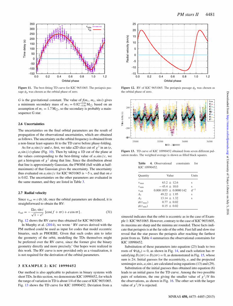
Figure 11. The best-fitting TD curve for KIC 9651065. The periapsis pas-sage φp was chosen as the orbital phase of zero.

G is the gravitational constant. The value of f(m1, m2, sin i) givesa minimum secondary mass of m2 = 0.82+0.04

−0.06 M� based on anassumption of m1 = 1.7 M�, so the secondary is probably a main-sequence G star.

2.6 Uncertainties

The uncertainties on the final orbital parameters are the result ofpropagation of the observational uncertainties, which are obtainedas follows. The uncertainty on the orbital frequency is obtained froma non-linear least-squares fit to the TD curve before phase-folding.

As for a1sin i/c and e, first, we take a2D slice cut of χ2 in an (e,a1sin i/c)-plane (Fig. 10). Then by taking a 1D cut of the plane atthe values corresponding to the best-fitting value of a1sin i/c, weget a histogram of χ2 along that line. Since the distribution aboutthat line is approximately Gaussian, the FWHM (full width at half-maximum) of that Gaussian gives the uncertainty. The uncertaintythus evaluated on a1sin i/c for KIC 9651065 is ∼5 s, and that on eis 0.02. The uncertainties on the other parameters are evaluated inthe same manner, and they are listed in Table 3.

2.7 Radial velocity

Since vrad = c dτ/dt, once the orbital parameters are deduced, it isstraightforward to obtain the RV:

vrad = −�a1 sin i√1 − e2

[cos(f + � ) + e cos � ] . (31)

Fig. 12 shows the RV curve thus obtained for KIC 9651065.In Murphy et al. (2014), we wrote ‘ RV curves derived with the

PM method could be used as input for codes that model eccentricbinaries, such as PHOEBE. Given that such codes aim to inferthe geometry of the orbit, modelling the TDs themselves mightbe preferred over the RV curve, since the former give the binarygeometry directly and more precisely.’ Our hopes were realized inthis work. The RV curve is now provided only as a visualization, itis not required for the derivation of the orbital parameters.

3 EX A M P L E 2 : K I C 1 0 9 9 0 4 5 2

Our method is also applicable to pulsators in binary systems withshort TDs. In this section, we demonstrate KIC 10990452, for whichthe range of variation in TD is about 1/4 of the case of KIC 9651065.Fig. 13 shows the TD curve for KIC 10990452. Deviation from a

Figure 12. RV of KIC 9651065. The periapsis passage φp was chosen asthe orbital phase of zero.

Figure 13. TD curve of KIC 10990452 obtained from seven different pul-sation modes. The weighted average is shown as filled black squares.



τmax 63.2 ± 12.6 sτmin − 45.4 ± 10.0 sνorb 0.008 1855 ± 0.0000 142 d−1

A1 49.22 ± 1.95 sA2 13.14 ± 1.32 sφ(τmax) 0.77 ± 0.02φ(τmin) 0.15 ± 0.02

sinusoid indicates that the orbit is eccentric as in the case of Exam-ple 1: KIC 9651065. However, contrary to the case of KIC 9651605,its maxima are sharp and the minima are rounded. These facts indi-cate that periapsis is at the far side of the orbit. Fast fall and slow risereveal that the star passes the periapsis after reaching the farthestpoint from us. Table 4 summarizes the observational constraints forKIC 10990452.

Substitution of these parameters into equation (23) leads to tworoots of �(φp) = 0, as shown in Fig. 14, and each solution has �

satisfying D1(� ) = D2(� ) = 0, as demonstrated in Fig. 15, whosesum is 2π. Initial guesses for the eccentricity, e, and the projectedsemimajor axis, a1sin i, are calculated using equations (13) and (29).

Substitution of the initial guesses thus obtained into equation (6)leads to an initial guess for the TD curve. Among the two possiblepairs of solutions, the one giving the smaller value of χ2/N fitsthe observations, as shown in Fig. 16. The other set with the largervalue of χ2/N is rejected.

MNRAS 450, 4475–4485 (2015)

at University of T



Dow

nloaded from



Figure 14. Same as Fig. 5, but for KIC 10990452.

Figure 15. Same as Fig. 6, but for KIC 10990452.

The best-fitting parameters are obtained by searching for theminimum of χ2/N as a function of (e, a1sin i). Fig. 17 shows a 2Dcolour map of χ2/N. The best-fitting parameters are summarized inTable 5, and the TD curve generated with these parameters is shownin Fig. 18. Finally, the RV curve is obtained as shown in Fig. 19.

As seen in the case of KIC 10990452, the present method isapplicable without any difficulty to pulsators in binary systemsshowing TD variations of several tens of seconds. Judging fromthe error bars in the observed TDs of Kepler pulsators, and fromthe binaries we have found so far, we are confident that the presentmethod is valid for stars showing TD variations exceeding ∼±20 s.While it may be possible to find binaries with even smaller TDvariations, such cases will be close to the noise level of the data

Figure 16. Same as Fig. 9 but for KIC 10990452. The green curve, gen-erated with one of the solutions of parameters giving the smaller value ofχ2/N, where N denotes the number of data points, fits the data well. On theother hand, the red curve generated with the other set of parameters has alarger value, so it is rejected. The periapsis passage φp was chosen as theorbital phase of zero.


Table 5. The best-fitting orbital parameters ofKIC 10990452.


νorb 0.008 190 ± 0.000 014 d−1

(a1sin i)/c 61.3 ± 8.0 se 0.55 ± 0.03φp 0.89 ± 0.02� 5.81 ± 0.05 radf(m1, m2, sin i) 0.01 658 ± 0.00 649 M�

Figure 18. The best-fitting TD curve for KIC 10990452. The periapsispassage φp was chosen as the orbital phase of zero.

MNRAS 450, 4475–4485 (2015)

at University of T



Dow

nloaded from


PM stars II 4483

Figure 19. RV of KIC 10990452. The periapsis passage φp was chosen asthe orbital phase of zero.

and may require external confirmation. The noise limit is discussedfurther in Section 4.

4 E X A M P L E 3 : T H E M O R E E C C E N T R I C C A S EO F K I C 8 2 6 4 4 9 2

Fig. 20 shows the TD curve for another star, KIC 8264492. Devia-tion from a sinusoid indicates that the orbit is highly eccentric, andthe number of harmonics to the orbital period visible in Fig. 21, aswell as their high amplitudes, confirm this. Let us see if our methodis valid for such a highly eccentric binary system. Its maxima aresharp and the minima are rounded, indicating that periapsis is at thefar side of the orbit. Fast fall and slow rise reveal that the star passesthe periapsis after reaching the farthest point from us.

Figure 20. TD curve of KIC 8264492 obtained from seven different pulsa-tion modes. The weighted average is shown as filled black squares.

Figure 21. Fourier transform of the TD curve of KIC 8264492 shown inFig. 20. Exact multiples of the orbital frequency (0.003 94 d−1) are indicated,showing the many harmonics and implying high eccentricity.



τmax 214.6 ± 42.9 sτmin − 132.5 ± 26.5 sνorb 0.003 9408 ± 0.0000 158 d−1

A1 159.90 ± 3.61 sA2 50.41 ± 3.61 sφ(τmax) 0.76 ± 0.02φ(τmin) 0.12 ± 0.02

Figure 22. Same as Fig. 5, �(φp) (red curve), but for KIC 8264492.

The orbital frequency, the amplitudes of the highest componentand the second one, and the orbital phases at the maximum andthe minimum of the TDs are deduced from the Fourier transform.They are summarized in Table 6. Substitution of these parametersinto equation (23) enables numerical root-finding of �(φp) = 0,as shown in Fig. 22. One root corresponds to the case (A) thatthe pulsating star in question passes the periapsis soon after thenearest point to us, and the other corresponds to the case (B) thatthe star passes the apoapsis just before the furthest point from us.Corresponding to the presence of two possible solutions of φp, thereare two solutions of � , which are explementary angles (see Fig. 23).

Substitution of the initial guesses thus obtained into equation (6)leads to an initial guess for the TD curve. As in the case ofKIC 9651605, among the two possible pairs of solutions, one ofthem generates a reasonable TD curve that fits the observations,while the other generates a TD curve that is an almost mirror imageof the observed TD curve, with a larger value of χ2/N (Fig. 24).The correct solution is consistent with qualitative expectations de-scribed at the beginning of this subsection; the periapsis of the staris at the far side of the orbit, and the star passes the periapsis afterreaching the farthest point from us, that is, 3π/2 < � < 2π.

Fig. 24 shows the TD curve, computed for the initial guesses,plotted with the observed TDs. The orbital phase of zero is chosenso that φp = 0. The data points of τ obs were vertically shifted by theamount λ, defined by equation (3), so that they match τ th. Unlike theearlier example of KIC 9651065, there remain systematic residualsin the TD curve for KIC 8264492.

The best-fitting parameter derived from a 2D colour map of χ2/N(Fig. 25) are summarized in Table 7, and Fig. 26 and Fig. 27 showthe TD curve and the RV curve generated with these parameters,respectively. Hence, with KIC8264492, we have demonstrated thevalidity and utility of the PM method, even for systems with higheccentricity.

MNRAS 450, 4475–4485 (2015)

at University of T



Dow

nloaded from



Figure 23. Same as Fig. 6 but for KIC 8264492. The upper panel is the casethat the periapsis is in the near side to us, while the lower panel indicatesthe case that the periapsis is in the far side from us.

Figure 24. Same as Fig. 9 but for KIC 8264492. The violet curve, generatedwith the parameters in the first line of Table 6, fits the data well. On theother hand, the red curve generated with the other set of parameters has alarger value of χ2/N, so it is rejected. The periapsis passage φp was chosenas the orbital phase of zero.

5 D ISCUSSION

In this work, we have primarily focussed on deriving full or-bital solutions for highly eccentric binaries. Our first example,KIC 9651065, was also studied in our previous work (Murphy et al.2014), and so a direct evaluation of the improvement in techniqueis possible.


Table 7. The best-fitting orbital parameters ofKIC 8264492 deduced from the observational con-straints listed in Table 6.


νorb 0.003 940 ± 0.000 016 d−1

(a1sin i)/c 204.8 ± 25.8 se 0.67 ± 0.04φp 0.80 ± 0.02� 5.28 ± 0.05 radf(m1, m2, sin i) 0.143 08 ± 0.05 410 M�

Figure 26. The best-fitting TD curve for KIC 8264492. The periapsis pas-sage φp was chosen as the orbital phase of zero.

Figure 27. Same as Fig. 12 but for KIC 8264492.

MNRAS 450, 4475–4485 (2015)

at University of T



Dow

nloaded from


PM stars II 4485

Table 8. Comparison of the uncertainties in the orbital parameters forKIC 9651065. (i) Those calculated here by fitting the TD data in this workversus (ii) those calculated through fitting RVs obtained by taking pairwisedifferences of the TD data in previous work.

Quantity Units Value ValueThis work Previous work

νorb d−1 0.003 684 ± 0.000 011 0.003 667 ± 0.000 016(a1sin i)/c s 183.2 ± 5.0 185.0 ± 10.0e 0.44 ± 0.02 0.47 ± 0.03� rad 2.11 ± 0.05 2.01 ± 0.30f(m1, m2, sin i) M� 0.0896 ± 0.0074 0.0916 ± 0.0108χ2/N 1.80 2.21

5.1 Improvement in technique

The improvement can be seen in two ways. Firstly, the quality ofthe fit of the theoretical TD curve to the data can be evaluatedin terms of the reduced χ2 parameter. The former method gave avalue of 2.21 for KIC 9651065, compared to 1.80 for the analyticalapproach presented in this work. Secondly, one can compare theuncertainties in the orbital parameters obtained by each method.Table 8 shows that smaller uncertainties, particularly in � , resultfrom fitting the TDs directly, rather than fitting the RVs obtained bypairwise differences of the TD data.

There are also new improvements in the elimination of systematicerrors. Previously, the eccentricity would be underestimated due tothe reliance on the approximation in equation (13) (equation 5 inMurphy et al. 2014). This was also strongly subject to noise spikesin the Fourier transform of the TDs. Now, that approximation isonly used as an initial guess, and the search for the minimum in theχ2 distribution obtains the best-fitting value more reliably.

5.2 Factors affecting the minimum measurable TD

The detection of the smallest companions, which give rise to thesmallest TDs, requires a thorough understanding of the dominantcontributors to the noise and how that noise can be mitigated.

There are many ways that the noise level is affected by the prop-erties of the pulsation and/or the sampling. The cadence of the ob-servations has little impact on the quoted 20-s limit because Keplerobservations were mostly made in a single cadence (long-cadenceat 30 min), though for stars with ample short-cadence (60-s) datathe phase errors can be reduced by a factor ∼5 (Murphy 2012). Thenoise can be reduced when the star oscillates in many modes, pro-viding they have similar amplitudes to the highest amplitude mode.The noise in the weighted average TDs is then reduced, though tak-ing the weighted average means that the inclusion of more modesof much lower amplitudes than the strongest mode does not help,since phase uncertainties scale inversely with amplitude. Also forthis reason, we do not consider modes with amplitudes below onetenth of that of the strongest mode in each star, and high-amplitudepulsators are clearly more favourable. Furthermore, we consider amaximum of nine modes per star due to diminishing return in com-putation time. Finally, it is noteworthy that the smallest detectableTD variation has no theoretical dependence on the orbital period,providing the orbit is adequately sampled.

6 C O N C L U S I O N S

We have developed upon our previous work (Murphy et al. 2014),where we showed how light arrival TDs can be obtained through

pulsational phase modulation of binary stars. Formerly, RVs werecalculated numerically from the TDs and the orbital parameterswere obtained from the RV curve. Here, we have shown how thesame orbital parameters are obtainable directly from the TDs. TheRV curve is now provided only as a visualization; it is not a necessarystep in solving the orbit.

We will be applying this method to the hundreds of classicalpulsators for which we have measured TDs with Kepler data, withthe aim of delivering a catalogue of TD and RV curves alongsideorbital parameters in the near future. We likewise encourage devel-opers and users of binary modelling codes to consider taking TDsas inputs.

AC K N OW L E D G E M E N T S

We are grateful to the entire Kepler team for such exquisite data.We would like to thank Tim Bedding for his suggestions and en-couragement to pursue a method that derives orbital parametersthrough direct fitting of the TDs. We thank the anonymous refereefor suggestions that improved this paper.

This research was supported by the Australian Research Council,and by the Japan Society for the Promotion of Science. Fundingfor the Stellar Astrophysics Centre is provided by the Danish Na-tional Research Foundation (grant agreement no. DNRF106). Theresearch is supported by the ASTERISK project (ASTERoseismicInvestigations with SONG and Kepler) funded by the EuropeanResearch Council (grant agreement no. 267864).

R E F E R E N C E S

Balona L. A., 2014, MNRAS, 443, 1946Brouwer D., Clemence G. M., 1961, Methods of Celestial Mechanics.

Academic Press, New YorkBuchler J. R., Goupil M.-J., Hansen C. J., 1997, A&A, 321, 159Freire P. C., Kramer M., Lyne A. G., 2001, MNRAS, 322, 885Freire P. C., Kramer M., Lyne A. G., 2009, MNRAS, 395, 1775Koen C., 2014, MNRAS, 444, 1486Murphy S. J., 2012, MNRAS, 422, 665Murphy S. J., Shibahashi H., Kurtz D. W., 2013, MNRAS, 430, 2986Murphy S. J., Bedding T. R., Shibahashi H., Kurtz D. W., Kjeldsen H., 2014,

MNRAS, 441, 2515Shibahashi H., Kurtz D. W., 2012, MNRAS, 422, 738Shibahashi H., Kurtz D. W., Murphy S. J., 2015, MNRAS, in press

This paper has been typeset from a TEX/LATEX file prepared by the author.

MNRAS 450, 4475–4485 (2015)

at University of T



Dow

nloaded from


deriving the orbital properties of pulsators in binary … the...deriving the orbital properties of...

Documents