derivatives debacles - federal reserve bank of st. louis
TRANSCRIPT
To avoid all mistakes in the conduct of great enterprises is beyondman’s powers. Plutarch, Lives: Fabius.
Derivatives DebaclesCase Studies of Large Losses in Derivatives Markets
Anatoli Kuprianov
R ecent years have witnessed numerous accounts of derivatives-relatedlosses on the part of established and reputable firms. These episodeshave precipitated concern, and even alarm, over the recent rapid growth
of derivatives markets and the dangers posed by the widespread use of suchinstruments.
What lessons do these events hold for policymakers? Do they indicate theneed for stricter government supervision of derivatives markets, or for new lawsand regulations to limit the use of these instruments? A better understandingof the events surrounding recent derivatives debacles can help to answer suchquestions.
This article presents accounts of two of the costliest and most highly pub-licized derivatives-related losses to date. The episodes examined involve thefirms of Metallgesellschaft AG and Barings PLC. Each account begins with areview of the events leading to the derivatives-related loss in question, followedby an analysis of the factors responsible for the debacle. Both incidents raisea number of public policy questions: Can government intervention stop suchincidents from happening again? Is it appropriate for the government even totry? And if so, what reforms are indicated? These issues are addressed at the endof each case study, where the lessons and public policy concerns highlightedby each episode are discussed.
Alex Mendoza assisted in the preparation of this article. Ned Prescott, John Walter, and JohnWeinberg provided valuable comments on earlier drafts. Any remaining errors or omissionsare the responsibility of the author. The views expressed are those of the author and do notnecessarily represent those of the Federal Reserve Bank of Richmond or the Federal ReserveSystem.
Federal Reserve Bank of Richmond Economic QuarterlyVolume 81/4 Fall 1995 1

2 Federal Reserve Bank of Richmond Economic Quarterly
1. RISK AND REGULATION IN DERIVATIVES MARKETS
Perhaps the most widely cited report on the risks associated with derivativeswas published in 1993 by the Group of Thirty—a group consisting of prominentmembers of the international financial community and noted academics. Thereport identified four basic kinds of risks associated with the use of derivatives.1
Market riskis defined as the risk to earnings from adverse movements in marketprices. Press accounts of derivatives-related losses have tended to emphasizemarket risk; but the incidents examined in this article illustrate the importance ofoperational risk—the risk of losses occurring as a result of inadequate systemsand control, human error, or management failure.
Counterparty credit riskis the risk that a party to a derivative contractwill fail to perform on its obligation. Exposure to counterparty credit risk isdetermined by the cost of replacing a contract if a counterparty (as a party toa derivatives contract is known) were to default.
Legal risk is the risk of loss because a contract is found not to be legallyenforceable. Derivatives are legal contracts. Like any other contract, they re-quire a legal infrastructure to provide for the resolution of conflicts and theenforcement of contract provisions. Legal risk is a prime public policy concern,since it can interfere with the orderly functioning of markets.
These risks are not unique to derivative instruments. They are the sametypes of risks involved in more traditional types of financial intermediation,such as banking and securities underwriting. Legal risk does pose special prob-lems for derivatives markets, however. The novelty of many derivatives makesthem susceptible to legal risk because of the uncertainty that exists over theapplicability of existing laws and regulations to such contracts.
Although the risks associated with derivatives are much the same as thosein other areas of finance, there nonetheless seems to be a popular perception thatthe rapid growth of derivatives trading in recent years poses special problemsfor financial markets. Most of these concerns have centered on the growth ofthe over-the-counter (OTC) derivatives market. As Stoll (1995) notes, concernabout the growth of OTC derivatives markets has arisen because these instru-ments are nonstandard contracts, without secondary trading and with limitedpublic price information. Moreover, OTC markets lack some of the financialsafeguards used by futures and options exchanges, such as margining systemsand the daily marking to market of contracts, designed to ensure that all marketparticipants settle any losses promptly. The absence of such safeguards, alongwith the complexity of many of the new generation of financial derivativesand the sheer size of the market, has given rise to concerns that the growth ofderivatives trading might somehow contribute to financial instability. Finally,
1 See Global Derivatives Study Group (1993).

A. Kuprianov: Derivatives Debacles 3
there is some concern among policymakers that the federal financial regulatoryagencies have failed to keep pace with the rapid innovation in OTC deriva-tives markets.2 Such concerns have only been reinforced by frequent reportsof derivatives-related losses in recent years.
The traditional rationale for regulating financial markets stems from con-cerns that events in these markets can have a significant impact on the econ-omy. Much of the present-day financial regulatory system in the United Statesevolved as a response to financial panics that accompanied widespread eco-nomic recessions and depressions. For example, the creation of the FederalReserve System was prompted in large part by the Panic of 1907; the adventof federal deposit insurance was a response to the thousands of bank failuresthat accompanied the Great Depression.
The present-day financial regulatory system has several goals. The mostimportant is to maintain smoothly functioning financial markets. A prime re-sponsibility of institutions like the Federal Reserve is to keep isolated events,such as the failure of a single bank, from disrupting the operation of financialmarkets generally. During the twentieth century, U.S. financial market regu-lation expanded to encompass at least two more goals. The creation of asystem of federal deposit insurance in 1933 gave the federal government astake in the financial condition of individual commercial banks, since a federalagency was now responsible for meeting a bank’s obligations to its insureddepositors in the event of insolvency. In addition, Congress enacted the Securi-ties Exchange Act to help protect investors by requiring firms issuing publiclytraded securities to provide accurate financial reports. The act created the Se-curities and Exchange Commission (SEC) to regulate the sales and tradingpractices of securities brokers, as well as to enforce the provisions of the lawmore generally.
Although financial market regulation deals largely with the problem ofmanaging risk, it cannot eliminate all risk. Risk is inherent in all economicactivity. Financial intermediaries such as commercial and investment banksspecialize in managing financial risks. Regulation can seek to encourage suchinstitutions to manage risks prudently, but it cannot eliminate the risks inherentin financial intermediation. There is a tension here. Regulators seek to reducethe risks taken on by the firms they regulate. At the same time, however, firmscannot earn profits without taking risks. Thus, an overzealous attempt to reducerisk could prove counterproductive—a firm will not survive if it cannot earnprofits.
Conventional wisdom views derivatives markets as markets for risk trans-fer. According to this view, derivatives markets exist to facilitate the transferof market risk from firms that wish to avoid such risks to others more willing
2 See U.S. General Accounting Office (1994).

4 Federal Reserve Bank of Richmond Economic Quarterly
or better suited to manage those risks. The important thing to note in thisregard is that derivatives markets do not create new risks—they just facilitaterisk management. Viewed from this perspective, the rapid growth of deriva-tives markets in recent years simply reflects advances in the technology of riskmanagement. Used properly, derivatives can help organizations reduce financialrisk. Although incidents involving large losses receive the most public attention,such incidents are the exception rather than the rule in derivatives markets.
Most public policy concerns center around the speculative use of deriva-tives. Speculation involves the voluntary assumption of market risk in the hopeof realizing a financial gain. The existence of speculation need not concern pol-icymakers as long as all speculative losses are borne privately—that is, onlyby those individuals or organizations that choose to engage in such activities.But many policymakers fear that large losses on the part of one firm maylead to a widespread disruption of financial markets. The collapse of Baringsillustrates some of the foundations for such concerns. In the case of an insuredbank, regulators discourage speculation because it can lead to losses that mayultimately become the burden of the government.3
A view implicit in many recent calls for more comprehensive regulation ofderivatives markets is that these markets are subject to only minimal regulationat present. But exchange-traded derivatives, such as futures contracts, have longbeen subject to comprehensive government regulation. In the United States, theSEC regulates securities and options exchanges while the Commodity FuturesTrading Commission (CFTC) regulates futures exchanges and futures brokers.Although OTC derivatives markets are not regulated by any single federalagency, most OTC dealers, such as commercial banks and brokerage firms, aresubject to federal regulation.4 As it happens, both incidents examined in thisarticle involve instruments traded on regulated exchanges. Any judgment as towhether these incidents indicate a need for more comprehensive regulation ofthese markets requires some understanding of just what happened in each case.
2. METALLGESELLSCHAFT
Metallgesellschaft AG (hereafter, MG) is a large industrial conglomerate en-gaged in a wide range of activities, from mining and engineering to trade andfinancial services. In December 1993, the firm reported huge derivatives-related
3 Recent losses by firms such as Gibson Greetings and Procter & Gamble have also raisedconcerns about sales practices and the disclosure of risks associated with complex financial deriva-tives. Neither of the cases examined in this study involves such concerns, however.
4 Many securities companies book their OTC derivatives through unregulated subsidiaries.Although these subsidiaries are not subject to formal SEC regulation, the largest brokerage firmshave agreed to abide by certain regulatory guidelines and to make regular disclosures to both theSEC and CFTC about their management of derivatives-related risks. See Taylor (1995a).
A. Kuprianov: Derivatives Debacles 5
losses at its U.S. oil subsidiary, Metallgesellschaft Refining and Marketing(MGRM). These losses were later estimated at over $1 billion, the largestderivatives-related losses ever reported by any firm at the time. The incidenthelped bring MG—then Germany’s fourteenth largest industrial corporation—to the brink of bankruptcy. After dismissing the firm’s executive chairman,Heinz Schimmelbusch, and several other senior managers, MG’s board of su-pervisors was forced to negotiate a $1.9 billion rescue package with the firm’s120 creditor banks (Roth 1994a, b).
MG’s board blamed the firm’s problems on lax operational control bysenior management, charging that “speculative oil deals . . . had plungedMetallgesellschaft into the crisis.”5 Early press reports on the incident echoedthis interpretation of events, but subsequent studies report that MGRM’s use ofenergy derivatives was an integral part of a combined marketing and hedgingprogram under which the firm offered customers long-term price guarantees ondeliveries of petroleum products such as gasoline and heating oil. Reports thatMG’s losses were attributable to a hedging program have raised a host of newquestions. Many analysts remain puzzled by the question of how a firm couldlose over $1 billion by hedging.
The Metallgesellschaft debacle has sparked a lively debate on the short-comings of the firm’s hedging strategy and the lessons to be learned from theincident. The ensuing account draws from a number of recent articles, notablyCulp and Hanke (1994); Culp and Miller (1994a, b, 1995a, b, c, d); Edwardsand Canter (1995a, b); and Mello and Parsons (1995a, b).
MGRM’s Marketing Program
In 1992, MGRM began implementing an aggressive marketing program inwhich it offered long-term price guarantees on deliveries of gasoline, heatingoil, and diesel fuels for up to five or ten years. This program included severalnovel contracts, two of which are relevant to this study. The first was a “firm-fixed” program, under which a customer agreed to fixed monthly deliveriesat fixed prices. The second, known as the “firm-flexible” contract, specified afixed price and total volume of future deliveries but gave the customer someflexibility to set the delivery schedule. Under the second program, a customercould request 20 percent of its contracted volume for any one year with 45days’ notice. By September 1993, MGRM had committed to sell forward theequivalent of over 150 million barrels of oil for delivery at fixed prices, withmost contracts for terms of ten years.
Both types of contracts included options for early termination. These“cash-out provisions” permitted customers to call for cash settlement on thefull volume of outstanding deliveries if market prices for oil rose above the
5 As cited in Edwards and Canter (1995b), p. 86.
6 Federal Reserve Bank of Richmond Economic Quarterly
contracted price. The firm-fixed contract permitted a customer to receive one-half the difference between the current nearby futures price (that is, the priceof the futures contract closest to expiration) and the contracted delivery price,multiplied by the entire remaining quantity of scheduled deliveries. The firm-flexible contract permitted a customer to receive the full difference between thesecond-nearest futures price and the contract price, multiplied by all remainingdeliverable quantities.6
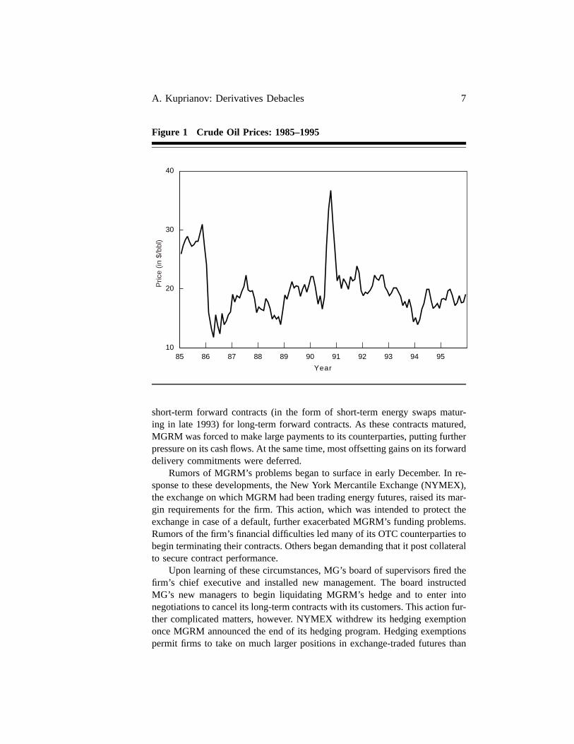
MGRM negotiated most of its contracts in the summer of 1993. Its con-tracted delivery prices reflected a premium of $3 to $5 per barrel over theprevailing spot price of oil. As is evident in Figure 1, energy prices were rela-tively low by recent historical standards during this period and were continuingto fall. As long as oil prices kept falling, or at least did not rise appreciably,MGRM stood to make a handsome profit from this marketing arrangement. Buta significant increase in energy prices could have exposed the firm to massivelosses unless it hedged its exposure.
MGRM sought to offset the exposure resulting from its delivery commit-ments by buying a combination of short-dated oil swaps and futures contractsas part of a strategy known as a “stack-and-roll” hedge. In its simplest form, astack-and-roll hedge involves repeatedly buying a bundle, or “stack,” of short-dated futures or forward contracts to hedge a longer-term exposure. Each stackis rolled over just before expiration by selling the existing contracts whilebuying another stack of contracts for a more distant delivery date; hence theterm stack-and-roll. MGRM implemented its hedging strategy by maintaininglong positions in a wide variety of contract months, which it shifted betweencontracts for different oil products (crude oil, gasoline, and heating oil) in amanner intended to minimize the costs of rolling over its positions.
Had oil prices risen, the accompanying gain in the value of MGRM’shedge would have produced positive cash flows that would have offset lossesstemming from its commitments to deliver oil at below-market prices. As ithappened, however, oil prices fell even further in late 1993. Moreover, declinesin spot and near-term oil futures and forward prices significantly exceeded de-clines in long-term forward prices. As a result, contemporaneous realized lossesfrom the hedge appeared to exceed any potential offsetting gains accruing toMGRM’s long-term forward commitments.
This precipitous decline in oil prices caused funding problems for MGRM.The practice in futures markets of marking futures contracts to market atthe end of each trading session forced the firm to recognize its futures trad-ing losses immediately, triggering huge margin calls. Normally, forward con-tracts have the advantage of permitting hedgers to defer recognition of losseson long-term commitments. But MGRM’s stack-and-roll hedge substituted
6 Mello and Parsons (1995b) provide a detailed description of these contracts.
A. Kuprianov: Derivatives Debacles 7
Figure 1 Crude Oil Prices: 1985–1995
85 86 87 88 89 90 91 92 93 94 9510
20
30
40
Pric
e (in
$/b
bl)
Year+
short-term forward contracts (in the form of short-term energy swaps matur-ing in late 1993) for long-term forward contracts. As these contracts matured,MGRM was forced to make large payments to its counterparties, putting furtherpressure on its cash flows. At the same time, most offsetting gains on its forwarddelivery commitments were deferred.
Rumors of MGRM’s problems began to surface in early December. In re-sponse to these developments, the New York Mercantile Exchange (NYMEX),the exchange on which MGRM had been trading energy futures, raised its mar-gin requirements for the firm. This action, which was intended to protect theexchange in case of a default, further exacerbated MGRM’s funding problems.Rumors of the firm’s financial difficulties led many of its OTC counterparties tobegin terminating their contracts. Others began demanding that it post collateralto secure contract performance.
Upon learning of these circumstances, MG’s board of supervisors fired thefirm’s chief executive and installed new management. The board instructedMG’s new managers to begin liquidating MGRM’s hedge and to enter intonegotiations to cancel its long-term contracts with its customers. This action fur-ther complicated matters, however. NYMEX withdrew its hedging exemptiononce MGRM announced the end of its hedging program. Hedging exemptionspermit firms to take on much larger positions in exchange-traded futures than

8 Federal Reserve Bank of Richmond Economic Quarterly
those allowed for unhedged, speculative positions. The loss of its hedgingexemption forced MGRM to reduce its positions in energy futures still further(Culp and Miller 1994b).
The actions of MG’s board of supervisors in this incident have spurredwidespread debate and criticism, as well as several lawsuits. Some analysts ar-gue that MGRM’s hedging program was seriously flawed and that MG’s boardwas right to terminate it. Others, including Nobel Prize-winning economistMerton Miller, argue that the hedging program was sound and that MG’s boardexacerbated any hedging-related losses by terminating the program prematurely.The discussion that follows reviews the hedging alternatives that were open tothe firm, the risks associated with the strategy it chose, and critiques of thatstrategy offered by a number of economists.
Hedging Alternatives
In common usage, the term “hedging” refers to an attempt to avoid the riskof loss by matching a given risk exposure with a counterbalancing risk, asin hedging a bet. Elementary finance textbooks are replete with examples ofperfect hedges, wherein a firm uses futures or forward contracts to offset per-fectly some given exposure. Hedging strategies employed by firms tend to besomewhat more complex, however. In practice, a perfect hedge can be difficultto arrange. And even when feasible, such a strategy often leaves little room forprofit.
Edwards and Canter (1995a, b) note that MGRM had at least three hedg-ing options open to it: physical storage, long-dated forward contracts, andsome variant of a stack-and-roll strategy. Physical storage would have requiredMGRM to purchase the oil products it had committed itself to deliver in thefuture and then store those products until the promised delivery dates. Physicalstorage would have been expensive, however. First, it would have requiredMGRM to finance the cost of the required inventories. Second, it would haveentailed the cost of the requisite storage facilities. Together, these two costscomprise what is known as the cost of carry. Available evidence suggests thatthe costs associated with physical storage would have rendered MGRM’s mar-keting program unprofitable.7
Alternatively, MGRM could have chosen among a number of derivatives-based hedging strategies involving either futures or forward contracts, or somecombination of both. Putting together a perfect hedge using such instrumentswould have required the purchase of a bundle of oil futures or forward contractswith expiration dates just matching MGRM’s promised delivery dates. But oilfutures typically trade only for maturities of three years or less. Moreover,liquidity tends to be poor for contracts with maturities over 18 months. Thus,MGRM would have had to buy a bundle of long-dated forward contracts from
7 See Edwards and Canter (1995a, b), and Mello and Parsons (1995b).
A. Kuprianov: Derivatives Debacles 9
an OTC derivatives dealer to put together a hedge that just offset its exposureto long-term energy prices.
Like physical storage, however, the cost associated with buying a bundleof long-dated forward contracts probably would have been prohibitive. To un-derstand why, note that buying a futures or forward contract is equivalent tophysical storage in the sense that both strategies ensure the future availabilityof an item at some predetermined cost. For this reason, the strategy of buyingfutures or forward contracts to lock in the cost of future delivery is sometimestermed “synthetic storage.” Accordingly, Arbitrage Pricing Theory predicts thatthe forward price for a commodity should reflect its cost of carry. Based on thefactors considered to this point, then, the theoretical no-arbitrage or benchmarkforward price should be
THEORETICAL FORWARD PRICE = SPOT PRICE + COST OF CARRY.
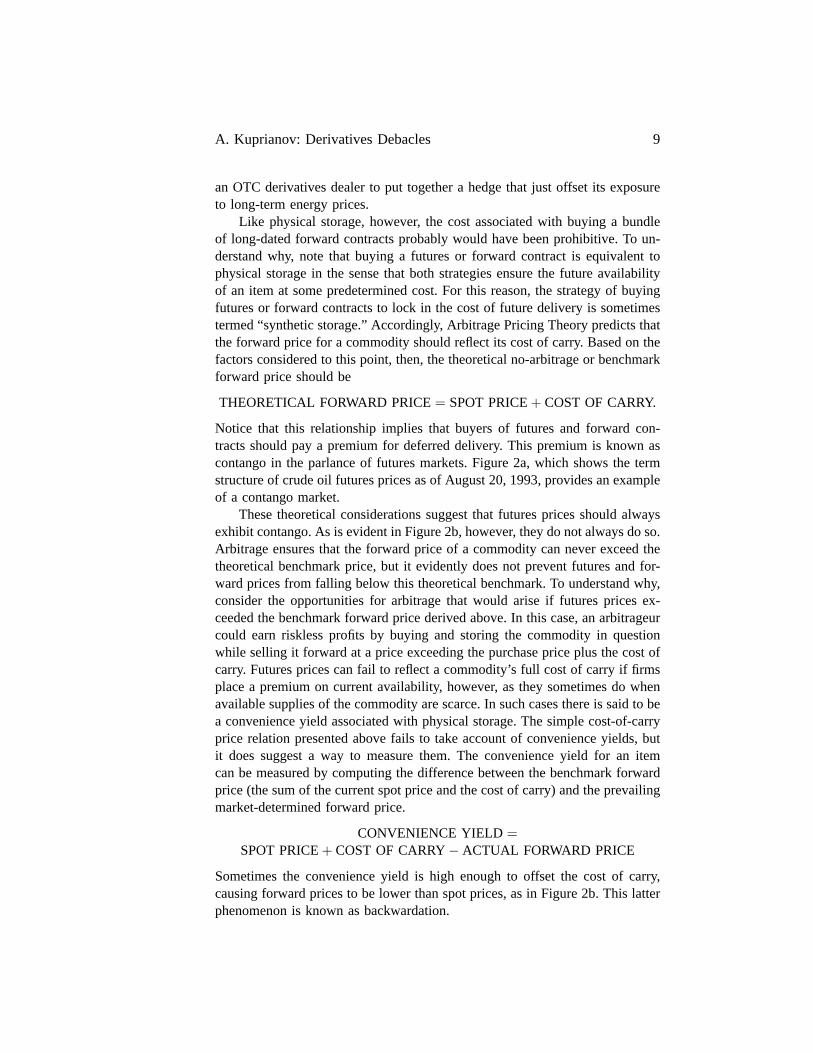
Notice that this relationship implies that buyers of futures and forward con-tracts should pay a premium for deferred delivery. This premium is known ascontango in the parlance of futures markets. Figure 2a, which shows the termstructure of crude oil futures prices as of August 20, 1993, provides an exampleof a contango market.
These theoretical considerations suggest that futures prices should alwaysexhibit contango. As is evident in Figure 2b, however, they do not always do so.Arbitrage ensures that the forward price of a commodity can never exceed thetheoretical benchmark price, but it evidently does not prevent futures and for-ward prices from falling below this theoretical benchmark. To understand why,consider the opportunities for arbitrage that would arise if futures prices ex-ceeded the benchmark forward price derived above. In this case, an arbitrageurcould earn riskless profits by buying and storing the commodity in questionwhile selling it forward at a price exceeding the purchase price plus the cost ofcarry. Futures prices can fail to reflect a commodity’s full cost of carry if firmsplace a premium on current availability, however, as they sometimes do whenavailable supplies of the commodity are scarce. In such cases there is said to bea convenience yield associated with physical storage. The simple cost-of-carryprice relation presented above fails to take account of convenience yields, butit does suggest a way to measure them. The convenience yield for an itemcan be measured by computing the difference between the benchmark forwardprice (the sum of the current spot price and the cost of carry) and the prevailingmarket-determined forward price.
CONVENIENCE YIELD =SPOT PRICE + COST OF CARRY − ACTUAL FORWARD PRICE
Sometimes the convenience yield is high enough to offset the cost of carry,causing forward prices to be lower than spot prices, as in Figure 2b. This latterphenomenon is known as backwardation.
10 Federal Reserve Bank of Richmond Economic Quarterly
Figure 2 Term Structure of Crude Oil Futures Prices
0 1 2 3 4 5 6 7 8 9 10 11 12 13 14 15 16 1718
18.5
19
19.5
20
Pric
e (in
$/b
bl)
0 1 2 3 4 5 6 7 8 9 10 11 12 13 14 15 16 1719.8
20.2
20.6
21
Pric
e (in
$/b
bl)
0 1 2 3 4 5 6 7 8 9 10 11 12 13 14 15 16 1716
16.2
16.4
16.6
16.8
17
Pric
e (in
$/b
bl)
Example of a Market in Contango
Example of a Market in Backwardation
Example of a Market Exhibit ingBoth Backwardation and Contango
a. As of August 20, 1993
b. As of August 21, 1992
c. As of April 20, 1994
Months to Expiration
Months to Expiration
Months to Expiration
+
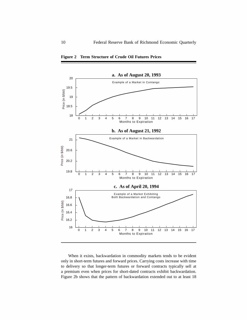
When it exists, backwardation in commodity markets tends to be evidentonly in short-term futures and forward prices. Carrying costs increase with timeto delivery so that longer-term futures or forward contracts typically sell ata premium even when prices for short-dated contracts exhibit backwardation.Figure 2b shows that the pattern of backwardation extended out to at least 18
A. Kuprianov: Derivatives Debacles 11
months as of August 21, 1992. At other times, however, futures prices beginincreasing at shorter horizons. Figure 2c shows the term structure of crude oilfutures prices as of April 20, 1994. On this latter date, futures prices exhibitedbackwardation only for the first four delivery months and then began rising.
The foregoing discussion shows that a hedging strategy based on long-term forward contracts can be almost as expensive as physical storage, evenwhen short-term futures and forward prices exhibit backwardation. So althoughMGRM could have hedged its exposure by buying long-term forward contractsfrom an OTC derivatives dealer, doing so would have reduced, if not elim-inated, any profits from its marketing program. Moreover, any dealer sellingsuch contracts would have faced similar hedging problems.
A stack-and-roll strategy appeared to offer a means of avoiding such carry-ing costs because short-dated futures markets for oil products historically havetended to exhibit backwardation. In markets that exhibit persistent backwarda-tion, a strategy of rolling over a stack of expiring contracts every month cangenerate profits. Thus, MGRM’s management apparently thought that a stack-and-roll hedging strategy offered a cost-effective means of locking in a spreadbetween current spot prices and the long-term price guarantees it had sold toits customers. As noted earlier, however, this strategy was not without risks.These risks are examined in more detail below.
Basis Risk
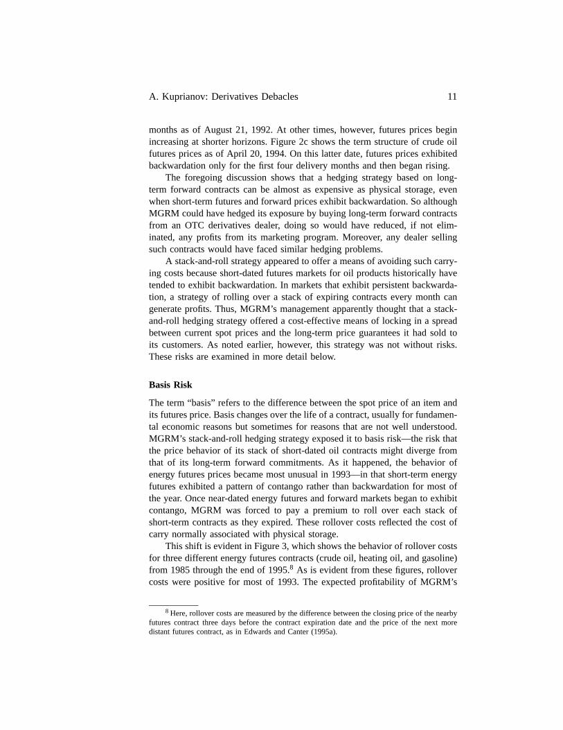
The term “basis” refers to the difference between the spot price of an item andits futures price. Basis changes over the life of a contract, usually for fundamen-tal economic reasons but sometimes for reasons that are not well understood.MGRM’s stack-and-roll hedging strategy exposed it to basis risk—the risk thatthe price behavior of its stack of short-dated oil contracts might diverge fromthat of its long-term forward commitments. As it happened, the behavior ofenergy futures prices became most unusual in 1993—in that short-term energyfutures exhibited a pattern of contango rather than backwardation for most ofthe year. Once near-dated energy futures and forward markets began to exhibitcontango, MGRM was forced to pay a premium to roll over each stack ofshort-term contracts as they expired. These rollover costs reflected the cost ofcarry normally associated with physical storage.
This shift is evident in Figure 3, which shows the behavior of rollover costsfor three different energy futures contracts (crude oil, heating oil, and gasoline)from 1985 through the end of 1995.8 As is evident from these figures, rollovercosts were positive for most of 1993. The expected profitability of MGRM’s
8 Here, rollover costs are measured by the difference between the closing price of the nearbyfutures contract three days before the contract expiration date and the price of the next moredistant futures contract, as in Edwards and Canter (1995a).

12 Federal Reserve Bank of Richmond Economic Quarterly
Figure 3
85 86 87 88 89 90 91 92 93 94 95-25
-20
-15
-10
-5
0
5
Cos
t (in
cen
ts/g
al)
Year
85 86 87 88 89 90 91 92 93 94 95-10
-5
0
5
10
Cos
t (in
cen
ts/g
al)
Year
85 86 87 88 89 90 91 92 93 94 95-2
-1
0
1
2
Cos
t (in
$/b
bl)
Year
Rollover Costs for Crude Oil Futures
Rollover Costs for Gasoline Futures
+
Rollover Costs for Heating Oil Futures
Note: Rollover costs are measured as of three days before contract expiration.
A. Kuprianov: Derivatives Debacles 13
combined marketing and hedging program was predicated on the assumptionthat energy futures markets would continue to exhibit a pattern of backwar-dation, however. MG’s board of supervisors apparently feared that the needto pay these rollover costs could add further to MGRM’s losses and chose toliquidate the subsidiary’s hedge and terminate its long-term delivery contractswith its customers.
Critiques of MGRM’s Hedging Program
As Figure 1 shows, oil prices began rising in 1994, soon after MGRM’s newmanagement lifted the firm’s hedge. It thus appears that MGRM could haverecouped most if not all of its losses simply by sticking to its hedging program.Whether management should have been able to anticipate this outcome is thetopic of an active debate, however.
Criticisms of MGRM’s hedging program have focused on two issues. Thefirst deals with the assumptions the architects of MGRM’s hedging strategymade regarding the likely future behavior of basis in oil futures and forwardmarkets. The second concerns the steps MGRM could have taken to reduce thevariability of its cash flows.
Both Edwards and Canter (1995a) and Mello and Parsons (1995b) showthat MGRM’s hedging program would have generated huge losses if contangoenergy markets had persisted throughout 1994. A key question, then, is whetherMG’s board of supervisors should have viewed the behavior of energy futuresprices during 1993 as a temporary aberration, or whether it had reasonablegrounds to believe that this price behavior could persist indefinitely.
Edwards and Canter conclude that permanent changes in the behavior ofbasis are possible and have occurred in other futures markets. As evidence,they cite experience with two other commodity futures contracts: soybeansand copper. Both markets were characterized by backwardation from 1965 to1975, but then began exhibiting persistent contango. Thus, while a stack-and-roll hedging strategy for either commodity would have produced positive cashflows on average before 1975, such a strategy would have lost money consis-tently over the ensuing ten-year period—meaning that a hedger employing astack-and-roll strategy of the type used by MGRM in either soybean or copperfutures markets would have experienced large and persistent losses after 1975.
Along with Mello and Parsons (1995a, b), Edwards and Canter (1995a,b) argue that MGRM was overhedged because short-term oil futures pricestend to be much more volatile than prices on long-term forward contracts.According to these authors, MGRM’s managers could have—and shouldhave—designed a hedge that would have reduced the variability of the firm’sshort-term cash flows. Edwards and Canter find that the correlation of short-term energy futures and forward prices with long-term prices is approximately50 percent. Thus, they argue that MGRM could have minimized the variance of
14 Federal Reserve Bank of Richmond Economic Quarterly
its cash flows with a hedge approximately 50 percent smaller than the total of itsfuture delivery commitments.9 Mello and Parsons observe that the exact size ofa minimum-variance hedge is difficult to calculate because MGRM’s contractsgave its customers options to terminate their contracts after three years. Theyfind that the minimum-variance hedge ratio could be as high as 75 percent ifone assumes that all such options would be exercised at the end of three years.
While critical of certain aspects of MGRM’s hedging strategy, Edwardsand Canter are agnostic as to whether MG’s board was correct to terminateits U.S. subsidiary’s oil-hedging program.10 Mello and Parsons (1995a, b) aremore critical of MGRM’s hedging strategy, arguing that it was speculative inits design and intent. They base their views on a written strategic plan preparedby MGRM’s management, which outlined a plan to exploit backwardation infutures markets as part of its hedging program. Where the plan went wrong,according to Mello and Parsons, was in assuming that the firm could take advan-tage of backwardation to price its long-term customer contracts below the fullcost of carry. They conclude that viewing MGRM’s stack-and-roll strategy asa hedge reverses the order of cause and effect, arguing that it should be viewedas a misguided speculative attempt to profit from the backwardation normallypresent in futures markets for petroleum products while using forward deliverycontracts as a partial hedge.
A Defense of MGRM’s Hedging Strategy
Culp and Miller (1994a, b, 1995a, b, c, d) and Culp and Hanke (1994) arecritical of MG’s board of supervisors for terminating MGRM’s marketing andhedging program. These authors argue that MGRM’s hedging strategy wassound and that the firm’s losses are attributable primarily to the way the boardterminated the program.
While acknowledging that the volatility of short-term oil prices did makeMGRM’s cash flows volatile, Culp and Miller argue that short-term cash flowvolatility is irrelevant to judgments about the efficacy of MGRM’s hedgingprogram. They base this argument on two considerations. The first stems froma theoretical analysis of the properties of a stack-and-roll hedge, the secondfrom a practical analysis of MG’s ability to continue funding the program.
First, Culp and Miller (1994b, 1995d) demonstrate that a stack-and-rollhedge of the type employed by MGRM will offset perfectly any changes in the
9 A 50 percent hedge ratio does not take into account that changes in the value of a long-term forward contract will not be realized for many years, however. The procedure for doing sois known as “tailing the hedge” (see Kawaller [1986] for a description). Tailing the hedge lowersthe recommended hedge ratio even further. Edwards and Canter estimate that MGRM could haveminimized the variance of its cash flows by buying short-term futures contracts for 61 millionbarrels of oil to hedge a 160 million barrel long-term exposure.
10 In a more recent article, however, Edwards (1995) is somewhat more critical of the decisionto liquidate MGRM’s forward delivery contracts.
A. Kuprianov: Derivatives Debacles 15
value of a long-term forward commitment so long as the factors determiningbasis—interest rates, storage costs, and the implicit convenience yield associ-ated with physical storage—do not change. Thus, according to Culp and Miller,it is misleading to blame MG’s losses on changes in the term structure of oilprices. While short-term price volatility can make cash flows volatile, it doesnot affect the net present value of the hedged exposure as long as basis remainsunchanged.
As noted earlier, however, the behavior of basis did change in the summerof 1993. Culp and Miller acknowledge that MGRM’s hedging strategy exposedthe firm to basis risk, but they argue that this risk was relatively small con-sidering the historical behavior of energy futures prices. Their analysis showsthat changes in basis affect only the portion of carrying costs borne by thehedger. The hedger bears no carrying costs as long as the convenience yieldis greater than or equal to the cost of carry—that is, when the market exhibitsbackwardation—but must bear at least some portion of carrying costs in acontango market. These carrying costs appear as rollover costs.
No one has attempted to refute Culp and Miller’s theoretical results. Rather,other authors question the presumption that oil markets would always tend toexhibit backwardation, whereas Culp and Miller argue that any long-run ex-pected losses due to basis risk were minimal considering historical patterns ofbackwardation in energy markets.
At first glance, the results of Culp and Miller’s analysis appear difficultto reconcile with the $1.3 billion loss auditors later attributed to MGRM’smarketing and hedging program. Culp and Miller (1995c) take issue with thisestimate, however, arguing that MG’s auditors underestimated the value ofMGRM’s contracts with its customers. They argue that taking proper accountof unrealized gains in the value of such contracts results in a net loss of $170million rather than $1.3 billion. According to Culp and Miller, most of MG’sreported losses were attributable to the manner in which its new managementchose to terminate its subsidiary’s marketing program, not to defects in itshedging strategy. It is not unusual for the parties to such agreements to nego-tiate termination of a contract before it expires. The normal practice in suchcircumstances involves payment by one party to the other to compensate for anychanges in the value of the contract. In contrast, it appears that MGRM’s newmanagement simply agreed to terminate its contracts with its customers withoutasking for any payment to reflect changes in the value of those contracts. Thehedge—however imperfect—effectively was transformed by this action into ahuge speculative transaction after the fact.
Although Culp and Miller do find that MGRM’s hedging program hadsuffered losses (albeit much smaller losses than those calculated by MG’sauditors), they argue that those losses did not justify terminating MGRM’shedging program. First, they emphasize that any past losses were sunk costs.At the same time, they find that the program had a positive expected net present
16 Federal Reserve Bank of Richmond Economic Quarterly
value at the end of 1993.11 Thus, they argue that the firm had good reason tocontinue the program. Culp and Miller reject the board’s argument that ter-minating MGRM’s hedge was the only way of dealing with the subsidiary’smassive cash outflows. They note that the firm could have bought options toremain hedged while it sought solutions to its longer-term funding problems.Moreover, they argue that short-term cash flow constraints should not havepresented any insurmountable problems in view of MG’s long-standing andclose relations with Deutsche Bank, Germany’s largest commercial bank. Theyemphasize that Deutsche Bank was not only a creditor to MG but also oneof its largest shareholders. In addition, a Deutsche Bank executive, RonaldoSchmitz, was chairman of MG’s board of supervisors at the time. Accordingly,Culp and Miller conclude that the Deutsche Bank should have been willing tocontinue financing MGRM’s hedge in view of its close relations with MG andits expertise in finance.
At the very least, Culp and Miller suggest, MG’s management could havebought options to hedge its oil exposure while seeking a longer-term solution toits funding problems, as suggested by MGRM’s management. As a longer-termsolution, they argue that the firm could have spun off the combined marketingand hedging program into a separate subsidiary, which could have been soldto another firm. This argument is supported by Edwards (1995), who reportsthat at least one major U.S. bank had offered to provide secured financing toMGRM based on a plan to securitize its forward delivery contracts.
Besides taking issue with the actions of MG’s board of supervisors, Culpand Hanke (1994) fault NYMEX for the actions the exchange took againstMGRM. They argue that these actions needlessly exacerbated MGRM’s tem-porary cash flow problems and thereby helped to precipitate a funding crisisfor the firm.
Reconciling Opposing Views
Disagreements over the efficacy of MGRM’s hedging program stem from dif-fering assumptions about (1) the goal of the hedging program (or, perhapsmore accurately, what the goal should have been), and (2) the feasibility ofcontinuing the program in light of the large negative cash flows MGRM ex-perienced in late 1993. Both Edwards and Canter (1995a, b) and Mello andParsons (1995a, b) emphasize the difficulties that the large negative cash flowsproduced by the hedging program caused the parent company. These authorsargue that MGRM’s management should have sought to avoid such difficultiesby designing a hedge that would have minimized the volatility of its cash flows.
Although they are critical of MGRM’s hedging strategy, Edwards andCanter offer no opinion as to whether MG’s board was right to terminate
11 Note, however, that this estimate is based on the assumption that expected carrying costswould be zero over the long run. See Culp and Miller (1995a, b, d).
A. Kuprianov: Derivatives Debacles 17
the program. Like Culp and Miller, they are puzzled about the decision toterminate existing contracts with customers without negotiating some paymentto compensate for the increase in the value of those contracts.
Mello and Parsons’s criticisms of MGRM’s hedging strategy are unequivo-cal. They argue that MGRM’s strategy was fatally flawed, and they defend thedecision to terminate the hedging program as the only means of limiting evengreater potential future losses. They also emphasize the difficulty that MG’s newmanagement would have had in securing the financing necessary to maintainMGRM’s hedging program and argue that funding considerations should haveled the subsidiary’s managers to synthesize a hedge using long-dated forwardcontracts. In this context, Mello and Parsons note that the parent firm alreadyhad accumulated a cash flow deficit of DM 5.65 billion between 1988 and1993. This deficit had been financed largely by bank loans. Considering thesecircumstances, they find the reluctance of MG’s creditor banks to fund thecontinued operation of the oil marketing program understandable.
Culp and Miller accept that MGRM’s hedge was intended to exploit thebackwardation normally present in energy futures markets, but they reject theargument that its hedging program represented reckless speculation. They em-phasize that few, if any, commodity dealers always hedge away all risks, citingthe results of previous studies on the behavior of commodity dealers to supporttheir assertions (Culp and Miller 1995a, b). Thus, they conclude that short-termcash flow constraints should not have presented any insurmountable problems inview of MG’s long-standing and close relations with Deutsche Bank, which theyfeel should have been willing to continue financing MGRM’s hedging program.
These disagreements over the efficacy of MGRM’s hedging strategy seemunlikely ever to be resolved, based as they are on different assumptions aboutthe goals management should have had for its strategy. The main issue, then, iswhether MG’s senior management and board of supervisors fully appreciatedthe risks the firm’s U.S. oil subsidiary had assumed. If they did, the firm shouldhave arranged for a line of credit to fund its short-term cash flows. Indeed, Culpand Miller (1995a, b, d) claim that MGRM had secured lines of credit withits banks just to prepare for such contingencies. Yet the subsequent behaviorof MG’s board suggests that its members had very little prior knowledge ofMGRM’s marketing program and were uncomfortable with its hedging strategy,despite the existence of a written strategic plan.
It is difficult for an outside observer to assign responsibility for any misun-derstandings between MG’s managers and its board of supervisors. MG’s boardultimately held Heinz Schimmelbusch, the firm’s executive chairman, respon-sible for the firm’s losses, claiming that he and other senior managers had lostcontrol over the activities of the firm and concealed evidence of losses.12 In
12 See The Wall Street Journal(1993) and The Economist(1993).

18 Federal Reserve Bank of Richmond Economic Quarterly
response, Schimmelbusch has filed suit against Ronaldo Schmitz and DeutscheBank, seeking $10 million in general and punitive damages (Taylor 1995b).Arthur Benson, former head of MGRM and architect of the firm’s ill-fatedhedging program, is suing MG’s board for $1 billion on charges of defamation(Taylor 1994). Thus, the issue of blame appears destined to be settled by theU.S. courts.
Response of the CFTC
The Metallgesellschaft debacle did not escape the attention of U.S. regula-tors. In July 1995, the U.S. Commodity Futures Trading Commission (CFTC)instituted administrative proceedings against MGRM and MG Futures, Inc.(MGFI), an affiliated Futures Commission Merchant that processed trades forMGRM and other MG subsidiaries.13 The CFTC order charged both MGRMand MGFI with “material inadequacies in internal control systems” associatedwith MGRM’s activity in energy and futures markets. In addition, MGFI wascharged with failing to inform the CFTC of these material inadequacies, whileMGRM was charged with selling illegal, off-exchange futures contracts. Thetwo MG subsidiaries settled the CFTC action without admitting or denying thecharges and agreed to pay the CFTC a $2.5 million settlement. They also agreedto implement a series of CFTC recommendations to reform their internal con-trols and to refrain from violating CFTC regulations. The CFTC’s action ren-dered MGRM’s firm-fixed agreements “illegal and void.”14 Thus, the CFTC’saction would have created legal risk for Metallgesellschaft and its customersexcept that the firm had already canceled most of the contracts in question.
The CFTC’s actions in this case have proven somewhat controversial.Under the Commodity Exchange Act, the CFTC is charged with regulatingexchange-traded futures contracts. At the same time, the act explicitly excludesordinary commercial forward contracts from the jurisdiction of the CFTC. Thelegal definition of a futures contract is open to differing interpretations, how-ever, leading to some uncertainty over the legal status of OTC derivatives underthe Commodity Exchange Act. Most market participants felt that this uncer-tainty was resolved in 1993 when, at the behest of Congress, the CFTC agreed toexempt off-exchange forward and swaps contracts from regulations governingexchange-traded contracts. CFTC chairman Mary Schapiro maintains that theagency’s action against MGRM does not represent a reversal of its policy onOTC contracts. According to Schapiro, the CFTC’s order is worded narrowlyso as to apply only to contracts such as the firm-fixed (45-day) agreements sold
13 A Futures Commission Merchant is a broker that accepts and executes orders for trans-actions on futures exchanges for customers. Futures Commission Merchants are regulated by theCFTC.
14 See U.S. Commodity Futures Trading Commission (1995a, b).

A. Kuprianov: Derivatives Debacles 19
by MGRM in this case.15 Nonetheless, this action has prompted some criticsto charge the agency with creating uncertainty about the legal status of com-mercial forward contracts. Critics of the action include Miller and Culp (1995)and Wendy Gramm, a former chairman of the CFTC.16 The CFTC’s actionhas also been criticized by at least two prominent members of Congress—Rep.Thomas J. Bliley, Jr., Chairman of the House Commerce Committee; and Rep.Pat Roberts, Chairman of the House Agricultural Committee.17
Since the CFTC’s action against Metallgesellschaft is narrowly directed andinvolves somewhat esoteric legal arguments, it is too soon to know what itseffect will be on OTC derivatives markets generally. Still, commodity dealersmust now take extra care in designing long-term delivery contracts to avoidpotential legal problems.18
An Overview of Policy Concerns
Considering the debate over the merits of MGRM’s hedging strategy, it wouldseem naive simply to blame the firm’s problems on its speculative use ofderivatives. It is true that MGRM’s hedging program was not without risks.But the firm’s losses are attributable more to operational risk—the risk of losscaused by inadequate systems and control or management failure—than tomarket risk. If MG’s supervisory board is to be believed, the firm’s previousmanagement lost control of the firm and then acted to conceal its losses fromboard members. If one sides with the firm’s previous managers (as well as withCulp, Hanke, and Miller), then the supervisory board and its bankers misjudgedthe risks associated with MGRM’s hedging program and panicked when facedwith large, short-term funding demands. Either way, the loss was attributableto poor management.
Does this episode indicate the need for new government policies or morecomprehensive regulation of derivatives markets? The answer appears to be no.MGRM’s losses do not appear ever to have threatened the stability of financialmarkets. Moreover, those losses were due in large part to the firm’s use offutures contracts, which trade in a market that is already subject to comprehen-sive regulation. The actions taken by the CFTC in this instance demonstrateclearly that U.S. regulators already have the authority to intervene when theydeem it necessary. Unfortunately, the nature of those actions in this case maycreate added legal risk for other market participants.
To view the entire incident in its proper perspective, it must be remem-bered that MG’s losses were incurred in connection with a marketing program
15 See BNA’s Banking Report(1995a).16 For a summary of Gramm’s comments see The Wall Street Journal(1995).17 See Fox (1995).18 See Rance (1995) for a legal analysis of these issues.

20 Federal Reserve Bank of Richmond Economic Quarterly
aimed at providing long-term, fixed-price delivery contracts to customers—atype of arrangement common to many types of commercial activity. Systematicattempts to discourage such arrangements would seem to be poor public policy.
Finally, MG’s financial difficulties were not attributable solely to its useof derivatives. As noted earlier, the firm’s troubles stemmed in part from theheavy debt load it had accumulated in previous years. Moreover, MGRM’soil marketing program was not the only source of its parent company’s lossesduring 1993. MG reported losses of DM 1.8 billion on its operations for thefiscal year ended September 30, 1993, in addition to the DM 1.5 billion lossauditors attributed to its hedging program as of the same date (Roth 1994a).Simply stated, the MG debacle resulted from poor management. As a practicalmatter, government policy cannot prevent firms such as Metallgesellschaft frommaking mistakes. Nor should it attempt to do so.
3. BARINGS
At the time of its demise in February 1995, Barings PLC was the oldestmerchant bank in Great Britain. Founded in 1762 by the sons of Germanimmigrants, the bank had a long and distinguished history. Barings had helpeda fledgling United States of America arrange the financing of the LouisianaPurchase in 1803. It had also helped Britain finance the Napoleonic Wars, afeat that prompted the British government to bestow five noble titles on theBaring family.
Although it was once the largest merchant bank in Britain, Barings wasno longer the powerhouse it had been in the nineteenth century. With totalshareholder equity of £440 million, it was far from the largest or most impor-tant banking organization in Great Britain. Nonetheless, it continued to rankamong the nation’s most prestigious institutions. Its clients included the Queenof England and other members of the royal family.
Barings had long enjoyed a reputation as a conservatively run institution.But that reputation was shattered on February 24, 1995, when Peter Baring,the bank’s chairman, contacted the Bank of England to explain that a trader inthe firm’s Singapore futures subsidiary had lost huge sums of money speculat-ing on Nikkei-225 stock index futures and options. In the days that followed,investigators found that the bank’s total losses exceeded US$1 billion, a sumlarge enough to bankrupt the institution.
Barings had almost failed once before in 1890 after losing millions inloans to Argentina, but it was rescued on that occasion by a consortium ledby the Bank of England. A similar effort was mounted in February 1995, butthe attempt failed when no immediate buyer could be found and the Bank ofEngland refused to assume liability for Barings’s losses. On the evening ofSunday, February 26, the Bank of England took action to place Barings into

A. Kuprianov: Derivatives Debacles 21
administration, a legal proceeding resembling Chapter 11 bankruptcy-court pro-ceedings in the United States. The crisis brought about by Barings’s insolvencyended just over one week later when a large Dutch financial conglomerate, theInternationale Nederlanden Groep (ING), assumed the assets and liabilities ofthe failed merchant bank.
What has shocked most observers is that such a highly regarded institutioncould fall victim to such a fate. The ensuing account examines the eventsleading up to the failure of Barings, the factors responsible for the debacle,and the repercussions of that event on world financial markets.19 This accountis followed by an examination of the policy concerns arising from the episodeand the lessons these events hold for market participants and policymakers.
Unauthorized Trading Activities
In 1992, Barings sent Nicholas Leeson, a clerk from its London office, tomanage the back-office accounting and settlement operations at its Singaporefutures subsidiary. Baring Futures (Singapore), hereafter BFS, was establishedto enable Barings to execute trades on the Singapore International MonetaryExchange (SIMEX). The subsidiary’s profits were expected to come primarilyfrom brokerage commissions for trades executed on behalf of customers andother Barings subsidiaries.20
Soon after arriving in Singapore, Leeson asked permission to take theSIMEX examinations that would permit him to trade on the floor of the ex-change. He passed the examinations and began trading later that year. Sometime during late 1992 or early 1993, Leeson was named general manager andhead trader of BFS. Normally the functions of trading and settlements arekept separate within an organization, as the head of settlements is expectedto provide independent verification of records of trading activity. But Leesonwas never relieved of his authority over the subsidiary’s back-office operationswhen his responsibilities were expanded to include trading.
19 This account is based on the findings of a report by the Board of Banking Supervision ofthe Bank of England (1995) and on a number of press accounts dealing with the episode. Exceptwhere otherwise noted, all information on this episode was taken from the Board of BankingSupervision’s published inquiry.
20 Most of BFS’s business was concentrated in executing trades for a limited number offinancial futures and options contracts. These were the Nikkei-225 contract, the 10-year Japan-ese Government Bond (JGB) contract, the three-month Euroyen contract, and options on thosecontracts (known as futures options). The Nikkei-225 contract is a futures contract whose valueis based on the Nikkei-225 stock index, an index of the aggregate value of the stocks of 225 ofthe largest corporations in Japan. The JGB contract is for the future delivery of ten-year Japanesegovernment bonds. The Euroyen contract is a futures contract whose value is determined bychanges in the three-month Euroyen deposit rate. A futures option is a contract that gives thebuyer the right, but not the obligation, to buy or sell a futures contract at a stipulated price on orbefore some specified expiration date.
22 Federal Reserve Bank of Richmond Economic Quarterly
Leeson soon began to engage in proprietary trading—that is, trading forthe firm’s own account. Barings’s management understood that such tradinginvolved arbitrage in Nikkei-225 stock index futures and 10-year Japanese Gov-ernment Bond (JGB) futures. Both contracts trade on SIMEX and the OsakaSecurities Exchange (OSE). At times price discrepancies can develop betweenthe same contract on different exchanges, leaving room for an arbitrageur toearn profits by buying the lower-priced contract on one exchange while sellingthe higher-priced contract on the other. In theory this type of arbitrage involvesonly perfectly hedged positions, and so it is commonly regarded as a low-riskactivity. Unbeknownst to the bank’s management, however, Leeson soon em-barked upon a much riskier trading strategy. Rather than engaging in arbitrage,as Barings management believed, he began placing bets on the direction ofprice movements on the Tokyo stock exchange.
Leeson’s reported trading profits were spectacular. His earnings soon cameto account for a significant share of Barings total profits; the bank’s seniormanagement regarded him as a star performer. After Barings failed, however,investigators found that Leeson’s reported profits had been fictitious from thestart. Because his duties included supervision of both trading and settlementsfor the Singapore subsidiary, Leeson was able to manufacture fictitious reportsconcerning his trading activities. He had set up a special account—accountnumber 88888—in July 1992, and instructed his clerks to omit information onthat account from their reports to the London head office. By manipulatinginformation on his trading activity, Leeson was able to conceal his tradinglosses and report large profits instead.
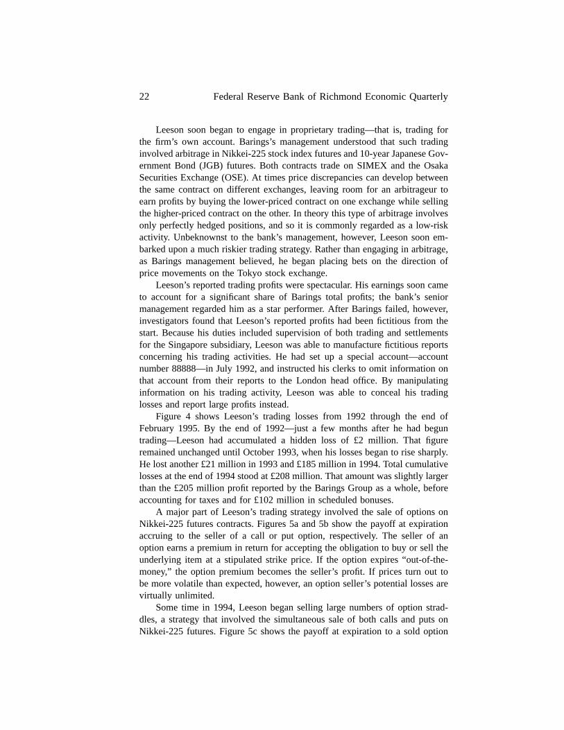
Figure 4 shows Leeson’s trading losses from 1992 through the end ofFebruary 1995. By the end of 1992—just a few months after he had beguntrading—Leeson had accumulated a hidden loss of £2 million. That figureremained unchanged until October 1993, when his losses began to rise sharply.He lost another £21 million in 1993 and £185 million in 1994. Total cumulativelosses at the end of 1994 stood at £208 million. That amount was slightly largerthan the £205 million profit reported by the Barings Group as a whole, beforeaccounting for taxes and for £102 million in scheduled bonuses.
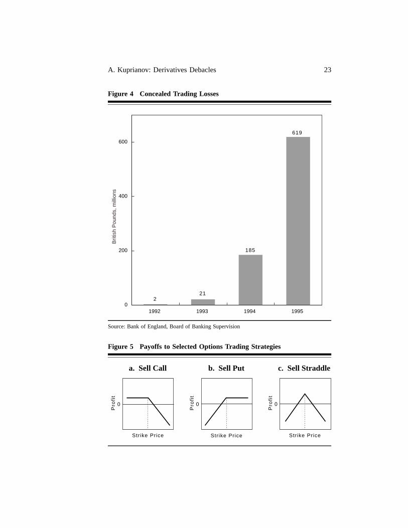
A major part of Leeson’s trading strategy involved the sale of options onNikkei-225 futures contracts. Figures 5a and 5b show the payoff at expirationaccruing to the seller of a call or put option, respectively. The seller of anoption earns a premium in return for accepting the obligation to buy or sell theunderlying item at a stipulated strike price. If the option expires “out-of-the-money,” the option premium becomes the seller’s profit. If prices turn out tobe more volatile than expected, however, an option seller’s potential losses arevirtually unlimited.
Some time in 1994, Leeson began selling large numbers of option strad-dles, a strategy that involved the simultaneous sale of both calls and puts onNikkei-225 futures. Figure 5c shows the payoff at expiration to a sold option
A. Kuprianov: Derivatives Debacles 23
Figure 4 Concealed Trading Losses
1992 1993 1994 19950
200
400
600
Brit
ish
Pou
nds,
mill
ions
221
185
619
+
Source: Bank of England, Board of Banking Supervision
Figure 5 Payoffs to Selected Options Trading Strategies
a. Sell Call c. Sell Straddle
Strike Price Strike Price Strike Price
b. Sell Put
Pro
fit
0
Pro
fit
0
Pro
fit
0
+
24 Federal Reserve Bank of Richmond Economic Quarterly
straddle. Option prices reflect the market’s expectation of the price volatilityof the underlying item. The seller of an option straddle earns a profit only ifthe market proves less volatile than predicted by option prices. As is evidentin Figure 5c, Leeson’s strategy amounted to a bet that the Japanese stockmarket would neither fall nor increase by a great deal—any large movement inJapanese stock prices would result in losses. By January 1, 1995, Leeson wasshort 37,925 Nikkei calls and 32,967 Nikkei puts. He also held a long positionof just over 1,000 contracts in Nikkei stock index futures, which would gainin value if the stock market were to rise.
Disaster struck on January 17 when news of a violent earthquake in Kobe,Japan, sent the Japanese stock market into a tailspin. Over the next five days,the Nikkei index fell over 1,500 points—Leeson’s options positions sustained aloss of £68 million. As stock prices fell, he began buying massive amounts ofNikkei stock index futures. He also placed a side bet on Japanese interest rates,selling Japanese government bond futures by the thousands in the expectationof rising interest rates.
This strategy seemed to work for a short time. By February 6, the Japan-ese stock market had recovered by over 1,000 points, making it possible forLeeson to recoup most of the losses resulting from the market’s reaction to theearthquake. His cumulative losses on that date totaled £253 million, about 20percent higher than they had been at the start of the year. But within days themarket began falling again—Leeson’s losses began to multiply. He continuedto increase his exposure as the market kept falling. By February 23, Leesonhad bought over 61,000 Nikkei futures contracts, representing 49 percent oftotal open interest in the March 1995 Nikkei futures contract and 24 percentof the open interest in the June contract. His position in Japanese governmentbond futures totaled just over 26,000 contracts sold, representing 88 percentof the open interest in the June 1995 contract. Leeson also took on positionsin Euroyen futures. He began 1995 with long positions in Euroyen contracts(a bet that Japanese interest rates would fall) but then switched to sellingthe contracts. By February 23 he had accumulated a short position inEuroyen futures equivalent to 5 percent of the open interest in the June 1995contract and 1 percent of the open interest in both the September and Decembercontracts.
Barings faced massive margin calls as Leeson’s losses mounted. Whilethese margin calls raised eyebrows at the bank’s London and Tokyo offices,they did not prompt an immediate inquiry into Leeson’s activities. It was notuntil February 6 that Barings’s group treasurer, Tony Hawes, flew to Singaporeto investigate irregularities with the accounts at BFS. Accompanying Haweswas Tony Railton, a settlements clerk from the London office.
While in Singapore, Hawes met with SIMEX officials, who had expressedconcern over Barings’s extraordinarily large positions. Hawes assured them thathis firm was aware of these positions and stood ready to meet its obligations
A. Kuprianov: Derivatives Debacles 25
to the exchange. His assurances were predicated on the belief that the firm’sexposure on the Singapore exchange had been hedged with offsetting positionson the Osaka exchange. He was soon to learn that this belief was incorrect.
Leeson’s requests for additional funding continued during February, andBarings’s London office continued to meet those requests—in all, Barings hadcommitted a total of £742 million to finance margin calls for BFS. Meanwhile,Tony Railton, the clerk Hawes had dispatched to Singapore, found that he couldnot reconcile the accounts of BFS. Particularly disturbing was a US$190 milliondiscrepancy in one of BFS’s accounts. For over a week, Railton attempted tomeet with Leeson to resolve these discrepancies. Leeson had become hard tofind, however. Railton finally tracked him down on the floor of the Singaporeexchange on Thursday, February 23, and persuaded Leeson to meet with himthat evening. When the meeting began, Railton began asking a series of difficultquestions. At that point Leeson excused himself, stating that he would returnshortly. But he never did return. Instead, he and his wife left Singapore thatevening. The next day, Leeson faxed his resignation to Barings’s London officefrom a hotel in Kuala Lumpur, stating in part, “My sincere apologies for thepredicament I have left you in. It was neither my intention nor aim for this tohappen.”21
After Leeson failed to return, Railton and others at Barings’s Singaporeoffice began investigating his private records and quickly discovered evidencethat he had lost astronomical sums of money. Peter Baring, the bank’s chairman,did not learn of the bank’s difficulties until the next day, when he was forcedto call the Bank of England to ask for assistance. Ironically, this was the sameday that Barings was to inform its staff of their bonuses. Leeson was to receivea £450,000 bonus, up from £130,000 the previous year, on the strength of hisreported profits. Baring himself expected to receive £1 million.
The Bank of England’s Board of Banking Supervision (1995) subsequentlyconducted an inquiry into the collapse of Barings. According to the Board’sreport, total losses attributable to Leeson’s actions came to £927 million (ap-proximately US$1.4 billion), including liquidation costs; an amount far inexcess of Barings total equity of £440 million. Most of the cost of the Baringsdebacle was borne by its shareholders and by ING, the firm that bought Barings.Barings was a privately held firm; most of its equity was held by the BaringFoundation, a charity registered in the United Kingdom. Barings’s executivecommittee held the firm’s voting shares, which constituted a small fraction ofthe firm’s total equity. Although ING was able to buy the failed merchant bankfor a token amount of £1, it had to pay £660 million to recapitalize the firm.SIMEX subsequently reported that the funds Barings had on deposit with theexchange were sufficient to meet the costs incurred in liquidating its positions
21 The full text of Leeson’s letter of resignation can be found in Springett (1995).
26 Federal Reserve Bank of Richmond Economic Quarterly
(Szala, Nusbaum, and Reerink 1995). It is not known whether the OSE sufferedany losses as a result of Barings’s collapse.
Leeson was later detained by authorities at the airport in Frankfort, Ger-many, and was extradited to Singapore the following November. In Singapore,Leeson pleaded guilty to charges of fraud and was sentenced to a 61⁄2-yearprison term (Mark 1995).
Certain material facts regarding the entire incident are not yet known, asLeeson refused to cooperate with British authorities unless extradited to GreatBritain. He later contested the findings of the Banking Board’s inquiry, however.A letter to the board from his solicitors states,
These conclusions are inaccurate in various respects. Indeed, in relation to cer-tain of the matters they betray a fundamental misunderstanding of the actualevents. Unfortunately, given the uncertainty regarding Mr. Leeson’s positionwe are not able to provide you with a detailed response to your letter.22
Leeson has promised to write a book describing his own version of eventswhile serving out his prison term in Singapore.
Market Aftershocks
Once the Singapore and Osaka exchanges learned that Barings would not beable to meet its margin calls, they took control of all the bank’s open positions.The Nikkei index fell precipitously when market participants learned that theexchanges would be liquidating such large positions. Thus, in the days imme-diately following the announcement of Barings’s collapse, it was not knownwhether the margin money the bank had deposited with the exchanges wouldcover the losses stemming from the liquidation of its positions.
Matters were further complicated when SIMEX announced it would dou-ble margin requirements on its Nikkei stock index futures contract effectiveTuesday, February 28. Fearing that their margin money might be used to payfor Barings’s losses, several of the exchange’s U.S. clearing members threat-ened to withhold payment of the additional margin SIMEX was demandingof them unless given assurances that such margin payments would be usedsolely to collateralize their own accounts. A refusal to pay would have causedthe affected dealers to forfeit their positions. If that had happened, SIMEXwould have been faced with a series of defaults. According to CFTC chairmanSchapiro, such an event could have “destroyed the ability of SIMEX to man-age the situation.”23 Indeed, there are reports that many market participantsfeared that the very solvency of the SIMEX clearinghouse was in question. Tocomplicate matters further, Japanese and Singaporean regulators were slow to
22 Board of Banking Supervision (1995), para. 1.77.23 As cited in McGee (1995b).
A. Kuprianov: Derivatives Debacles 27
inform market participants of the steps they were taking to insure the financialintegrity of the exchange clearinghouses. This lack of communication servedonly to exacerbate the fears of market participants (Falloon 1995; Irving 1995;McGee 1995b, c; Szala, Nusbaum, and Reerink 1995).
Upon learning of the situation, Chairman Schapiro contacted the MonetaryAuthority of Singapore (MAS) to persuade the agency to assure SIMEX’sclearing members that their margin deposits would not be used to offset Bar-ings’s proprietary losses. The MAS subsequently acceded to these requests andprovided its assurance in a short statement released before the start of tradingon Tuesday. SIMEX’s margin calls were met and a potential crisis was avoided.
This was not the end of headaches for Barings’s customers, however. BFSwas one of the largest clearing member firms on SIMEX. As such, it handledclearing and settlement for 16 U.S. firms and held approximately $480 millionin margin funds on their behalf when it went bankrupt.
U.S. futures exchanges typically arrange the immediate transfer to otherfirms of all customer accounts of a financially troubled clearing member. Lawsin the United States facilitate such transfers because they provide for strictsegregation of customer accounts, which prevents the creditors of a broker orclearing member firm from attaching the assets of customers. That Japaneselaw contains no such provisions was not well known before the collapse ofBarings. Although laws in Singapore do recognize the segregation of accounts,SIMEX had never before dealt with the insolvency of a clearing member firm.To complicate matters further, most of BFS’s customer accounts had beenbooked through Baring Securities in London. Consequently, SIMEX did nothave detailed information on individual customer positions. It had records onlyon a single commingled account for Baring Securities. Finally, much of theinformation that Leeson had provided to the exchange, as well as to Barings’sother offices, was false. These circumstances made the task of sorting out thepositions of individual customers extremely difficult.
During the next week, Barings’s U.S. customers scrambled to reproducedocumentation of their transactions with the bank and supplied this informationto SIMEX and the OSE. But while this information made it possible for theexchanges to identify customer positions, Barings’s bankruptcy administratorin London had asked the exchanges to block access to all Barings’s margin de-posits. The bankruptcy administrator had raised questions about whether U.K.laws on the segregation of customer accounts were applicable in an insolvencyof this kind (Szala, Nusbaum, and Reerink 1995).
It was not until ING took over Barings on March 9 that the bank’s cus-tomers were assured of access to their funds. Even then, access was delayedin many cases. By one account, several major clients waited more than threeweeks before their funds were returned (Irving 1995).

28 Federal Reserve Bank of Richmond Economic Quarterly
Policy Concerns Highlighted by Barings’s Default
All futures exchanges maintain systems to prevent the accumulation of largespeculative losses. But events surrounding the collapse of Barings have servedto highlight weaknesses in risk management on the part of SIMEX and otherfutures exchanges. They also suggest a need for closer international cooperationamong futures exchanges and their regulators, and for clearer laws on the statusof customer accounts when a clearing member firm becomes insolvent.
Futures exchanges maintain stringent speculative position limits for indi-vidual firms and traders to prevent large losses and to limit their exposure. Itappears that SIMEX relaxed some of these restrictions for BFS, however. It isnot unusual for futures exchanges to grant exemptions to established positionlimits for hedged positions, such as those Leeson claimed to maintain. But it isnormal for the exchange clearinghouse to monitor closely the activities of firmsreceiving such exemptions and to take steps to verify the existence of offsettingexposures. It now appears that SIMEX failed to pursue such precautions in itsdealings with Barings.
The exchange’s attitude toward Barings was influenced in part by thebank’s strong international reputation, but its willingness to relax normal riskmanagement guidelines also may have been attributable to its desire to attractbusiness. Although the OSE was first to list Japanese government bond andNikkei-225 stock index futures, SIMEX soon began listing similar contractsin direct competition with the Osaka exchange. Thereafter, the two exchangesbattled each other for market share. Barings was one of the most active firmson SIMEX—and Leeson was responsible for much of the exchange’s tradingvolume in Nikkei stock index futures and options. Thus, some observers believethat SIMEX may have been too willing to accommodate BFS (McGee 1995c).Critics include representatives of U.S. futures exchanges, who maintain thattheir risk management standards are more stringent.24 A report on the incidentcommissioned by the government of Singapore came to a similar conclusion,finding that the exchange may have been too liberal in granting increases inposition limits.25
Communication between exchanges can be important for identifying andresolving potential problems. Communication between SIMEX and the OSEwas minimal, however. This lack of communication not only helped make itpossible for Leeson to accumulate large losses but also hampered efforts tocontain the damage once Barings collapsed. Although the OSE routinely pub-lished a list of the positions of its most active traders, SIMEX did not makesuch disclosures. It now seems apparent that SIMEX officials never consulted
24 See BNA’s Banking Report(1995f) and Falloon (1995).25 See The Economist(1995).

A. Kuprianov: Derivatives Debacles 29
the OSE’s list to verify Leeson’s claim that he was hedging his large positionsin Singapore with offsetting exposures on the Osaka exchange.
Some observers blame this lack of communication on the rivalry betweenthe two exchanges. Arrangements existing between U.S. exchanges suggestthat competition need not preclude information sharing, however. In the UnitedStates, futures exchanges attempt to coordinate their activities with the CFTCand other futures exchanges. Each exchange maintains strict speculative posi-tion limits established under CFTC oversight. The CFTC monitors compliancethrough a comprehensive surveillance policy that includes a large-trader report-ing system. Market participants are required to justify unusually large positions.This system enabled the CFTC to ascertain quickly that Barings had no signif-icant positions on any U.S. futures exchange at the time of its collapse.26
While competitive concerns may sometimes give exchanges incentives torelax prudential standards, as many observers seem to think that SIMEX did,it does not follow that regulators should seek to discourage such competition.Competition among exchanges serves an important economic function by en-couraging innovation. Securities and futures exchanges constantly compete withone another to provide new products to their customers. Thus, whereas futuresexchanges once listed contracts only for agricultural and other commodities, asignificant fraction of all futures trading today involves contracts for financialinstruments. The growth of trading in such instruments has provided importantbenefits to international financial markets, helping to make them more efficientwhile facilitating risk management by financial intermediaries and commercialfirms alike. Moreover, competition gives futures exchanges an incentive tomaintain strong financial controls and risk management systems, as most mar-ket participants seek to avoid risks like those faced by SIMEX customers afterthe collapse of Barings. Finally, policymakers need not restrict competition toaddress the problems highlighted by the Barings debacle.
The events surrounding the collapse of Barings led futures industry regula-tors from 16 nations to meet in Windsor, England, in May 1995 to discuss theneed for legal and regulatory reform. At that meeting, officials agreed on a planof action now known as the Windsor Declaration. The declaration calls for reg-ulators to promote, as appropriate, “national provisions and market proceduresthat facilitate the prompt liquidation and/or transfer of positions, funds and as-sets, from failing members of futures exchanges,” and to support measures “toenhance emergency procedures at financial intermediaries, market members andmarkets and to improve existing mechanisms for international co-operation andcommunication among market authorities and regulators.”27 The InternationalOrganization of Securities Commissions (IOSCO) later endorsed the Windsor
26 See the summary of Chairman Schapiro’s testimony before Congress in BNA’s BankingReport(1995e, f).
27 As cited in BNA’s Banking Report(1995d).
30 Federal Reserve Bank of Richmond Economic Quarterly
Declaration and pledged to study the issues it raised. IOSCO also asked itsmembers to promote declaration measures in cross-border transactions.28
The Barings debacle has also spurred efforts by market participants tostrengthen financial safeguards at futures and options exchanges. In March1995, the Futures Industry Association (FIA) organized a task force to in-vestigate measures to improve the financial integrity of futures and optionsexchanges. The association’s Global Task Force on Financial Integrity (1995)subsequently published a report containing 60 recommendations, ranging fromrisk management practices to customer protection issues. The FIA report en-courages all nations to review their bankruptcy laws to clarify the status ofcustomer funds and to modify provisions that might conflict with the lawsof other nations. It recommends that exchanges and their regulators establishprocedures for the transfer of a troubled clearing member firm’s customer assetsbefore it is declared insolvent, as is now typically done in the United States.In addition, the report encourages exchange clearinghouses to monitor theirclearing member firms closely and to perform periodic audits. Thus, the FIA’srecommendations are broadly consistent with the principles espoused by theWindsor Declaration, especially in their emphasis on customer protection andthe need for improved information sharing among exchanges and governmentauthorities.
Subsequently, the clearing organizations for 19 U.S. stock, stock option,and futures exchanges announced their intent to begin pooling data on transac-tions of member firms (McGee 1995a). In addition, CFTC Chairman Schapirohas announced that her staff will work with the futures industry to developconcrete customer protection proposals.29
The Barings debacle has served to galvanize an international effort—onethat has been joined by government officials and market participants alike—toreevaluate risk management systems, customer protection laws, and proce-dures for dealing with the failure of a large clearinghouse member. It also hasprompted increased communication and pledges of greater cooperation amongregulators from different nations. It is still too early to pass judgment on theultimate success of such initiatives, however. While regulators have pledgedincreased international cooperation, recent press accounts have noted that of-ficials in Britain, Japan, and Singapore have not always cooperated with oneanother in conducting their investigations of the Barings case.30
Lessons from the Barings Debacle
The losses suffered by Barings provide a good example of the market riskassociated with derivatives. But, as with the case of Metallgesellschaft, the
28 See BNA’s Banking Report(1995b).29 See BNA’s Banking Report(1995c).30 See The Economist(1995).

A. Kuprianov: Derivatives Debacles 31
Barings debacle best illustrates operational risk and legal risk. In this regard,the Bank of England’s Board of Banking Supervision inquiry concluded,
Barings’ collapse was due to the unauthorized and ultimately catastrophicactivities of, it appears, one individual (Leeson) that went undetected as aconsequence of a failure of management and other internal controls of themost basic kind. Management failed at various levels and in a variety of ways. . . to institute a proper system of internal controls, to enforce accountabilityfor all profits, risks and operations, and adequately to follow up on a numberof warning signals over a prolonged period.31
The board’s inquiry found nine separate warning signs that should havealerted Barings management to problems with its Singapore futures subsidiary.A partial list of those warning signs includes the following:
• The lack of segregation of duties between front and back offices. This lackwas identified as a weakness and potential problem area in an internal auditreport following a review of BFS’s operations in the summer of 1994.Barings’s management failed to act on the report’s recommendations toremedy this situation.
• The high level of funding requested by Leeson.Between December 31,1994, and February 24, 1995, Barings provided Leeson with £521 millionto meet margin calls. Total funding of BFS stood at £742 million, more thantwice the reported capital of the Barings Group, when Leeson’s activitieswere finally discovered on February 24.32
• The unreconciled balance of funds transferred to BFS to meet margin calls.In his requests for additional funding, Leeson often claimed the moneywas needed for client accounts but never provided detailed informationabout these accounts as was the usual practice. Nonetheless, the bank’s headoffice in London paid those funds without any independent check on thevalidity of Leeson’s requests and with no attempt to reconcile thoserequests with known trading positions. Perhaps the most troubling aspect ofBarings’s behavior in this regard is that SIMEX rules prohibit its membersfrom financing the margin accounts of customers. Barings’s managementapparently ignored evidence that the firm might be doing so in violationof SIMEX rules.
• The apparent high profitability of Leeson’s trading activities relative tothe low level of risk as perceived and authorized by Barings’s managementin London. High returns typically entail high risk. Yet no one in seniormanagement seriously questioned how Leeson’s strong reported profits
31 Board of Banking Supervision (1995), para. 14.1.32 Board of Banking Supervision (1995), para. 6.21.
32 Federal Reserve Bank of Richmond Economic Quarterly
could result from what was supposed to have been a low-risk activity.To be sure, at least one executive observed that “This guy must be bustinghis intraday limits or something.”33 But Leeson’s reports were never chal-lenged until too late, and management did little to restrain his tradingactivities. According to interviews with Barings’s staff, Leeson was re-garded as “almost a miracle worker,” and there was “a concern not to doanything which might upset him.”34
• The discovery of discrepancies in Leeson’s accounts by outside auditors.Barings’s auditors, the firm of Coopers & Lybrand, informed the bank’smanagement of a £50 million discrepancy in BFS’s accounts on orbefore February 1, 1995. Although this discrepancy ultimately did promptBarings’s treasurer to investigate Leeson’s accounts, the Board of BankingSupervision concluded that management was too slow in responding to thiswarning sign.
• Communications from SIMEX.The rapid buildup of Leeson’s positionsduring January 1995 prompted SIMEX to seek assurances from Barings’smanagement in London regarding the ability of BFS to fund its margincalls. In retrospect, it appears that Barings’s management was too hastyin providing such assurances.
• Market rumors and concerns made known to Barings’s management inJanuary and February.By late January, rumors were circulating on theOSE regarding Barings’s large positions in Nikkei futures. On January 27,the Bank for International Settlements in Basle, Switzerland, raised a high-level inquiry with Barings executives in London regarding a rumor thatthe bank had experienced losses and could not meet its margin calls onthe OSE. On the same day, another Barings executive received a call fromthe Bloomberg information service inquiring into the bank’s large posi-tions on the OSE.
Taken together, these warning signs suggest that Barings’s management hadample cause to be concerned about Leeson’s activities. But management wastoo slow to act on these warning signs. An on-site examination of Leeson’saccounts came too late to save the bank.
The Board of Banking Supervision’s report outlined a number of lessonsto be learned from the failure of Barings. They emphasize five lessons for themanagement of financial institutions:
• Management teams have a duty to understand fully the businesses theymanage;
33 Board of Banking Supervision (1995), para. 3.57.34 Board of Banking Supervision (1995), para. 7.12.

A. Kuprianov: Derivatives Debacles 33
• Responsibility for each business activity has to be clearly establishedand communicated;
• Clear segregation of duties is fundamental to any effective control system;
• Relevant internal controls, including independent risk management, have tobe established for all business activities;
• Top management and the Audit Committee have to ensure that significantweaknesses, identified to them by internal audit or otherwise, are resolvedquickly.35
The report also had some criticisms for the Bank of England’s supervisionof Barings. U.K. banking regulations require all banks to notify the Bank ofEngland before entering into a transaction that would expose more than 25percent of the organization’s capital to the risk of loss. A Bank of Englandmanager granted Barings an informal concession permitting it to exceed thislimit in its exposure to SIMEX and the OSE without first referring the matterto the Bank’s senior management. But while the report is somewhat critical ofthe Bank of England on this matter, it concludes,
The events leading up to the collapse of Barings do not, in our view, ofthemselves point to the need for any fundamental change in the frameworkof regulation in the UK. There is, however, a need for improvements in theexisting arrangements.36
The report goes on to suggest a number of ways to improve the Bank ofEngland’s supervision of banks. According to the report,
• the Bank should explore ways of increasing its understanding of thenon-banking businesses . . . undertaken by those banks for which it isresponsible;37
• it should prepare explicit internal guidelines to assist its supervisory staffin identifying activities that could pose material risks to banks and ensurethat adequate safeguards are in place;
• it should work more closely with the Securities and Futures Authority, theagency responsible for regulating the domestic operations of British-basedsecurities firms, as well as with regulators from other nations; and
• it should address deficiencies in the implementation of rules dealing withlarge exposures.
35 Board of Banking Supervision (1995), para. 14.2.36 Board of Banking Supervision (1995), para. 14.5.37 Board of Banking Supervision (1995), para. 14.35.
34 Federal Reserve Bank of Richmond Economic Quarterly
The report also recommended an independent quality assurance review of theBank of England’s supervisory function.
The Board of Banking Supervision’s report did not blame the collapse ofBarings on its use of derivatives. Instead, it placed responsibility for the debacleon poor operational controls at Barings:
The failings at Barings were not a consequence of the complexity of thebusiness, but were primarily a failure on the part of a number of individualsto do their jobs properly....While the use of futures and options contracts didenable Leeson to take much greater levels of risk (through their leverage)than might have been the case in some other markets, it was his ability to actwithout authority and without detection that brought Barings down.38
This point has been reinforced recently by news of a similar debacle at theNew York office of Daiwa Bank, where a trader concealed large trading lossesfor over ten years before finally confessing to his activities.39 Parallels betweenthe Daiwa and Barings debacles are striking, as both incidents resulted fromthe unauthorized activities of a single trader. Daiwa’s losses were in no wayrelated to derivatives, however. The bank incurred over $1 billion in losses asa result of unauthorized trading in U.S. government bonds, widely regarded asthe safest of financial instruments.
Some Final Observations on the Barings Debacle
The events surrounding the collapse of Barings have highlighted certain weak-nesses in international financial markets that represent legitimate concerns forpolicymakers. The most notable of these weaknesses relate to (1) the lackof communication between securities and futures exchanges and regulators indifferent countries, and (2) conflicting laws on the legal status of customeraccounts at futures brokers and clearing agents in the event of insolvency.These weaknesses can be addressed only by increased international cooperationamong futures exchanges, regulators, and lawmakers.
At the same time, it does not appear that more stringent government reg-ulation of futures markets could have prevented the Barings debacle. Leesonacted outside existing regulatory guidelines and outside the law in concealingthe true nature of his trading activities and the losses resulting therefrom. Ex-isting laws and regulations should have been able to prevent, or at least todetect, Leeson’s activities before he could incur such astronomical losses. ButBarings, SIMEX, and the Bank of England were all lax in enforcing thoserules. Barings was lax in enforcing basic operational controls. In doing so,it violated not only official regulations but also commonly accepted marketstandards for managing risk. Similarly, it appears that SIMEX may have been
38 Board of Banking Supervision (1995), para. 14.35.39 See Sapsford, Sesit, and O’Brien (1995) for early details of the Daiwa debacle.

A. Kuprianov: Derivatives Debacles 35
too liberal in granting increases in position limits to BFS. Finally, the Bank ofEngland granted Barings an exemption that helped make it possible for Leesonto continue his illicit activities undetected.
4. CONCLUDING COMMENTS
The cases of Metallgesellschaft and Barings provide an interesting study incontrasts. Both cases involve exchange-traded derivatives contracts. In bothcases, senior management has been criticized for making an insufficient effortto understand fully the activities of their firms’ subsidiaries and for failing tomonitor and supervise the activities of those subsidiaries adequately. But whilecritics have faulted MG’s management for overreacting to the large margincalls faced by one of its subsidiaries, Barings’s management has been faultedfor being overly complacent in the face of a large number of warning signs.
If these two disparate incidents offer any single lesson, it is the need forsenior management to understand the nature of the firm’s activities and the risksthat those activities involve. In the case of Metallgesellschaft, the sheer scaleof its U.S. oil subsidiary’s marketing program exposed the firm to large risks.Although there is a great deal of disagreement over the efficacy of the hedgingstrategy employed by MGRM, it would seem difficult to argue that membersof MG’s board of supervisors fully appreciated the nature or magnitude of therisks assumed by the firm’s U.S. oil subsidiary. If they had, they would nothave been so shocked to find the firm facing large margin calls. In the case ofBarings, senior management seemed content to accept that a single trader couldearn huge profits without exposing the firm to large risks. With the benefit ofhindsight, it seems clear that senior executives of both firms should have takenmore effort to understand the activities of subordinates.
News of derivatives-related losses often prompts calls for more compre-hensive regulation of derivatives markets. But the cases of Metallgesellschaftand Barings—which rank among the largest derivatives-related losses to date—involve instruments traded in markets already subject to comprehensive regu-lation. In the case of Barings, the debacle involved a regulated merchant banktrading in regulated futures markets. If anything, the Barings debacle illus-trates the limits of regulation. Established rules and regulations should havebeen able to prevent a single trader from accumulating catastrophic losses. Butboth SIMEX and the Bank of England granted exemptions that helped makeit possible for Leeson to continue his activities for years without being de-tected. It appears that regulatory organizations can also be subject to operationalweaknesses.
Moreover, the instruments traded by these two firms—oil futures, stock in-dex futures, and stock index options—are not the kinds of complex and exoticinstruments responsible for concerns often expressed in connection with the

36 Federal Reserve Bank of Richmond Economic Quarterly
growth of derivatives markets. In the case of Barings, the Bank of England’sBoard of Banking Supervision concluded that it was not the complexity of thebusiness but the failure of a large number of individuals to do their jobs properlythat made the bank susceptible to catastrophic losses by a single trader. As therecent misfortune of Daiwa Bank shows, weaknesses in operational controlscan lead to losses in many areas of a firm’s operations, not just those involvedwith derivatives. The losses suffered by Daiwa resulted from trading in U.S.Treasury bonds, widely regarded as the safest of all securities.
Unfortunately, no amount of regulation can remove all risk from financialmarkets. Risk is inherent in all economic activity, and financial markets exist tohelp market participants diversify such risks. At the same time, regulation canimpose costs on market participants. The Metallgesellschaft case shows thatattempts at stringent regulation can sometimes have undesirable side effects.According to critics, the CFTC’s action against MG’s U.S. subsidiaries hasintroduced uncertainty about the legal status of commercial forward contracts.As a general rule, government policy should attempt to minimize legal riskrather than create it.
To be sure, the Barings debacle did highlight the need for certain legal andregulatory reforms and for more international cooperation among exchangesand their regulators. But market discipline is also a powerful form of regula-tion. Highly publicized accounts of derivatives-related losses have led manyfirms to scrutinize their risk management practices—not only in the area ofderivatives, but in other areas of their operations as well. Thus, while it is truethat derivatives debacles often reveal the existence of disturbing operationalweaknesses among the firms involved, such incidents can also teach lessonsthat help to make financial markets safer in the long run. As the foregoingaccounts show, regulation cannot substitute for sound management practices.At the same time, government policymakers can act to minimize the potentialfor disruption to financial markets by promoting laws and policies that minimizelegal risk.
REFERENCES
BNA’s Banking Report. “Schapiro Defends CFTC Action against Two MGSubsidiaries,” vol. 65 (September 25, 1995a), p. 503.
. “IOSCO Endorses Value-at-Risk Models for Capital AdequacyCalculations,” vol. 65 (July 17, 1995b), pp. 120–21.
. “Schapiro Says CFTC, Industry to Craft Customer ProtectionProposals,” vol. 65 (July 3, 1995c), pp. 15–16.

A. Kuprianov: Derivatives Debacles 37
. “World Futures Regulators Adopt Plan of Action in View ofBarings,” vol. 64 (May 22, 1995d), pp. 1017–18.
. “CFTC Undertaking Regulatory Review: Schapiro Address[es]Failure of Barings PLC,” vol. 64 (March 6, 1995e), pp. 469–70.
. “CFTC Chairman Schapiro Tells Congress Barings-Type DisasterUnlikely in U.S.,” vol. 64 (March 6, 1995f), pp. 468–69.
Board of Banking Supervision. Report of the Board of Banking SupervisionInquiry into the Circumstances of the Collapse of Barings. London:HMSO, 1995.
Culp, Christopher L., and Steve H. Hanke. “Derivative Dingbats,” TheInternational Economy(July/August 1994).
Culp, Christopher L., and Merton H. Miller. “Basis Risk and HedgingStrategies: Reply to Mello and Parsons,” Derivatives Quarterly,vol. 1(Summer 1995a), pp. 20–26.
. “Hedging in the Theory of Corporate Finance: A Reply to OurCritics,” Journal of Applied Corporate Finance,vol. 8 (Spring 1995b),pp. 121–27.
. “Auditing the Auditors,” Risk,vol. 8 (April 1995c), pp. 36–39.
. “Metallgesellschaft and the Economics of Synthetic Storage,”Journal of Applied Corporate Finance,vol. 7 (Winter 1995d), pp. 62–76.
. “Letter to the Editor,” Risk,vol. 11 (November 1994a), p. 18.
. “Hedging a Flow of Commodity Deliveries with Futures: Lessonsfrom Metallgesellschaft,” Derivatives Quarterly,vol. 1 (Fall 1994b), pp.7–15.
The Economist. “The Barings Collapse: Spot the Smoking Receivable,”October 21, 1995, p. 79.
. “Revolution at Metallgesellschaft,” December 25, 1993, p. 90.
Edwards, Franklin R. “Derivatives Can Be Hazardous to Your Health: TheCase of Metallgesellschaft,” Derivatives Quarterly,vol. 1 (Spring 1995),pp. 8–17.
, and Michael S. Canter. “The Collapse of Metallgesellschaft:Unhedgeable Risks, Poor Hedging Strategy, or Just Bad Luck?” TheJournal of Futures Markets,vol. 15 (May 1995a), pp. 211–64.
. “The Collapse of Metallgesellschaft: Unhedgeable Risks, PoorHedging Strategy, or Just Bad Luck?” Journal of Applied CorporateFinance,vol. 8 (Spring 1995b), pp. 86–105.
Falloon, William. “Who’s Missing from the Picture?” Risk,vol. 8 (April 1995),pp. 19–22.
Fox, Justin. “2 in House Fault Futures Trading Panel on Over-the-CounterDerivatives Ruling,” American Banker,December 26, 1995.

38 Federal Reserve Bank of Richmond Economic Quarterly
Futures Industry Association Global Task Force on Financial Integrity.Financial Integrity Recommendations. Washington: Futures IndustryAssociation, 1995.
Global Derivatives Study Group. Derivatives: Practices and Principles.Washington: Group of Thirty, 1993.
Irving, Richard. “Beyond Barings,” Risk,vol. 8 (April 1995), p. 6.
Kawaller, Ira. “Hedging with Futures Contracts: Going the Extra Mile,”Journal of Cash Management,vol. 6 (July/August 1986), pp. 34–36.
Mark, Jeremy. “With Leeson in Singapore Prison, Focus Shifts to BaringsExecutives,” The Wall Street Journal,December 4, 1995.
McGee, Suzanne. “Nineteen U.S. Exchanges To Share Data on Dealings,” TheWall Street Journal,September 6, 1995a.
. “New U.S. Futures Chief Is Crafting a Global Role,” The WallStreet Journal,May 17, 1995b.
. “Reform Sought to Prevent Future Barings,” The Wall StreetJournal, March 17, 1995c.
Mello, Antonio S., and John E. Parsons. “Hedging a Flow of CommodityDeliveries with Futures: Problems with a Rolling Stack,” DerivativesQuarterly, vol. 1 (Summer 1995a), pp. 16–19.
. “Maturity Structure of a Hedge Matters: Lessons from theMetallgesellschaft Debacle,” Journal of Applied Corporate Finance,vol.8 (Spring 1995b), pp. 106–20.
Miller, Merton H., and Christopher L. Culp. “Rein in the CFTC,” The WallStreet Journal,August 17, 1995.
Rance, Brian D. “The Commodity Futures Trading Commission Order ofSettlement with MG Refining and Marketing, Inc. and MF Futures, Inc.,”Derivatives Quarterly,vol. 2 (Winter 1995), pp. 13–17.
Roth, Terrence. “German Firm’s Bailout Package Gets Approved,” The WallStreet Journal,January 17, 1994a.
. “Metallgesellschaft Sets Shareholder Vote Despite Worries overFinancial Package,” The Wall Street Journal,January 14, 1994b.
Sapsford, Jathon, Michael R. Sesit, and Timothy L. O’Brien. “How DaiwaBond Man in New York Cost Bank $1.1 Billion in Losses,” The WallStreet Journal,September 27, 1995.
Springett, Pauline. “The Barings Rescue: ‘Apologies, but the pressures havebecome too much to bear,’ ” The Guardian(London), March 7, 1995.
Stoll, Hans R. “Lost Barings: A Tale in Three Parts Concluding with a Lesson,”The Journal of Derivatives,vol. 3 (Fall 1995), pp. 109–15.
Szala, Ginger, David Nusbaum, and Jack Reerink. “Barings Abyss,” Futures,vol. 24 (May 1995), pp. 68–74.

A. Kuprianov: Derivatives Debacles 39
Taylor, Jeffrey. “Securities Firms Agree to Set Controls on Derivatives,” TheWall Street Journal,March 9, 1995a.
. “Documents at MG Appear to Contradict Fired Chairman’s Stanceon Derivatives,” The Wall Street Journal,January 27, 1995b.
. “MG Corp. Aims to Stay Active in Oil Business,” The Wall StreetJournal, March 14, 1994.
U.S. Commodity Futures Trading Commission. “Order Instituting ProceedingsPursuant to Sections 6(c) and 8(a) of the Commodity Exchange Act andFindings and Order Imposing Remedial Sanctions,” CFTC Docket No.95-14 (1995a).
. “CFTC Order Imposes $2.25 Million Civil Penalty against MGRefining and Marketing, Inc. and MG Futures, Inc.; Other Remedial Sanc-tions Include Review of Internal Control Systems for Risk Management,”Release No. 3859-95 (July 27, 1995b).
U.S. General Accounting Office. Financial Derivatives: Actions Needed toProtect the Financial System.GAO/GCD-94-133, May 1994.
The Wall Street Journal.“Former CFTC Chief Scores Agency’s Move inDerivatives Case,” December 1, 1995.
. “Metallgesellschaft A.G. Dismisses Chairman and Finance Chief,”December 20, 1993.


Was the Disinflation of theEarly 1980s Anticipated?
Michael Dotsey and Jed L. DeVaro
T he United States experienced a rise in inflation from 5.5 percent inthe first quarter of 1976 to 9.4 percent in the first quarter of 1980.This steep increase was followed by the desire to stem inflation and to
reverse its course. Therefore, soon after Paul Volcker was appointed chairmanof the Federal Reserve Board in August 1979, the Federal Reserve (the Fed)announced new operating procedures and put in place a disinflationary policy.
During the implementation of that policy, two recessions came in rapidsuccession. The first began in January 1980 and lasted through the middle ofthat year. Although short in duration, the recession was deep, with real GDPfalling at an annual rate of 10.4 percent in the second quarter of 1980, the largestpostwar decline on record. The second recession followed almost immediately,beginning in July 1981 and ending in November 1982. At approximately thesame time, the Fed’s aggressive disinflationary policy ended. Some economistshave calculated the cost in terms of cumulative output lost to be roughly 24percent of total output over the period 1980:1 to 1983:4.1 But during thatperiod, inflation was brought down from 10.1 percent in 1980 to 4.4 percentin 1982.
This episode was dramatic because of both the significant loss of output andthe equally significant decline in inflation. Also, the policy of disinflation wasannounced and was carried out over a period of three years. Thus, the episodehas the potential to shed light on a number of competing macroeconomictheories that attempt to explain the linkage between real economic activity and
We wish to thank Alan Stockman for suggesting this topic. We are also indebted to JamesHamilton for many helpful discussions and for providing the programs that with slight mod-ifications were used in the statistical analysis. Mary Finn, Tom Humphrey, Peter Ireland, andRoy Webb contributed a number of useful suggestions. The views expressed are those of theauthors and do not necessarily reflect those of the Federal Reserve Bank of Richmond or theFederal Reserve System.
1 Using somewhat different procedures, both Fischer (1986) and Ball (1993) arrive at thisconclusion.
Federal Reserve Bank of Richmond Economic Quarterly Volume 81/4 Fall 1995 41

42 Federal Reserve Bank of Richmond Economic Quarterly
nominal disturbances. The usefulness of the 1980’s experience in this purposedepends critically on whether the decline in inflation was anticipated. If thedisinflation was largely unexpected, even after the policy had been in place forsome time, then it will be difficult to discriminate between the theories.
The first set of theories can broadly be classified as Keynesian and arecharacterized by elements of nominal rigidities in prices and wages. Specif-ically, we have in mind models like those of Fischer (1977), Taylor (1980),or Ball, Mankiw, and Romer (1988). In these models, staggered price settingslows the adjustment of the price level to changes in the money stock. Thus,inflation has inertia, and anticipated monetary contractions can precipitate arecession by causing aggregate demand to fall. The fall in aggregate demandwill of course be greater if the disinflationary policy is unanticipated, sinceeven those firms in the process of resetting their prices will make mistakes.
Other models in which unanticipated changes in monetary policy have aneffect on real economic activity are the neoclassical monetary business-cyclemodels of Lucas (1973), McCallum (1980), and Sargent and Wallace (1975). Inthese models, agents partially infer nominally induced movements in prices asbeing driven by real disturbances. Thus, an unanticipated fall in money causesprices to be lower than expected, resulting in a decline in the supply of output.If policy is anticipated, however, and there is no confusion about the impulsesdriving prices, agents are not induced to supply less output. The entire effectof policy is nominal.
Economists have varying opinions concerning the extent to which disin-flation was anticipated during the 1980-83 period, and these views partiallydetermine their preferred theory. For example, in discussing a number of pol-icy changes, including the one in which we are interested, Akerlof, Rose, andYellen (1988) argue that
Mr. Volcker’s similar policy produced changes in equilibrium output long afterthe policies were announced (and seem to be credible). The changes persistedsufficiently long after their announcement that it is extraordinarily difficult tobelieve that the changes in employment and output they caused were due tothe slow propagation of unanticipated shocks. (P. 68)
Their view is that the Fed possessed sufficient credibility, implying that thepolicy change was believed either immediately or soon thereafter and hencethat the disinflation was largely anticipated. If that was indeed the case, thentheir conclusion that the episode was more in line with Keynesian-style theoriesthan neoclassical ones is well taken.
The degree of Fed credibility, and hence the extent to which the disinflationwas anticipated, is open to question. Goodfriend (1992), in his description ofthe Fed’s fight against inflation, divides the period into three distinct parts: theaborted fight against inflation from October 1979 to April 1980, when short-term interest rates rose by over 600 basis points; an easing of policy during

M. Dotsey and J. L. DeVaro: Disinflation of the Early 1980s 43
the first recession, when rates fell by 800 basis points; and a second aggres-sive disinflationary policy from August 1980 to October 1982, when rates wereeventually pushed up by 1000 basis points over their July 1980 levels. This lastsustained tightening broke the inflationary environment. Thus Federal Reservepolicy was far from uniform and this lack of uniformity may have impairedthe Fed’s credibility, implying that the disinflation could very well have beenunanticipated. Thus, how well the public anticipated the disinflation can helpmeasure the Federal Reserve’s credibility during that period.
1. DESCRIPTION OF THE 1976−−1983 PERIOD
We begin with a brief overview of the period in question, confining ourselvesto a description of the behavior of inflation, real GDP growth, M1 growth, andthe federal funds rate (see Figures 1a to 1c). Inflation is measured by quarterlychanges in the GDP deflator and all quarterly growth rates are annualized.
As Figure 1a illustrates, the period was characterized by a run-up in in-flation from 5.5 percent in 1976:1 to 11.1 percent in 1981:1 and then by arapid decline to 4.09 percent in 1983:4. Associated with this rapid disinflationwere two recessions (Figure 1b). The first one began in January 1980 andwas accompanied by a 10.4 percent annualized decline in real GDP during thesecond quarter of that year, and the second one began in July 1981.
Figure 1a GDP Deflator Inflation: 1970 to 1986
70:1 72:1 74:1 76:1 78:1 80:1 82:1 84:1 86:10
2
4
6
8
10
12
14
Per
cent
+
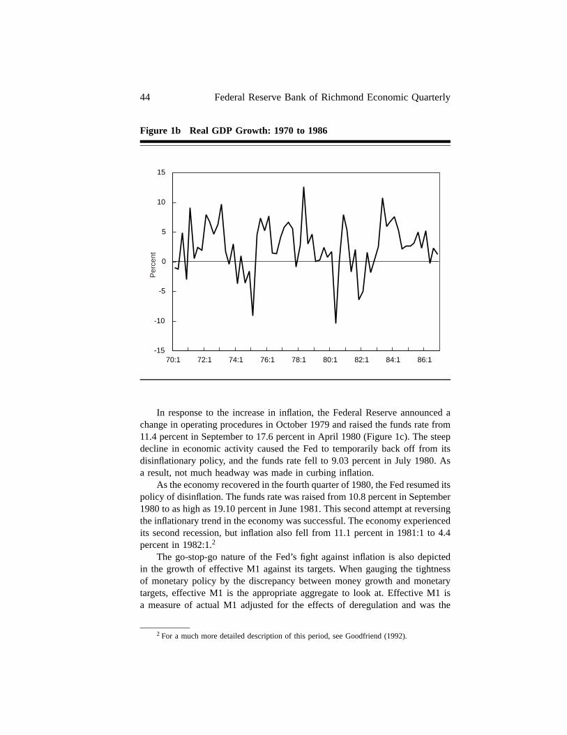
44 Federal Reserve Bank of Richmond Economic Quarterly
Figure 1b Real GDP Growth: 1970 to 1986
70:1 72:1 74:1 76:1 78:1 80:1 82:1 84:1 86:1-15
-10
-5
0
5
10
15
Per
cent
+
In response to the increase in inflation, the Federal Reserve announced achange in operating procedures in October 1979 and raised the funds rate from11.4 percent in September to 17.6 percent in April 1980 (Figure 1c). The steepdecline in economic activity caused the Fed to temporarily back off from itsdisinflationary policy, and the funds rate fell to 9.03 percent in July 1980. Asa result, not much headway was made in curbing inflation.
As the economy recovered in the fourth quarter of 1980, the Fed resumed itspolicy of disinflation. The funds rate was raised from 10.8 percent in September1980 to as high as 19.10 percent in June 1981. This second attempt at reversingthe inflationary trend in the economy was successful. The economy experiencedits second recession, but inflation also fell from 11.1 percent in 1981:1 to 4.4percent in 1982:1.2
The go-stop-go nature of the Fed’s fight against inflation is also depictedin the growth of effective M1 against its targets. When gauging the tightnessof monetary policy by the discrepancy between money growth and monetarytargets, effective M1 is the appropriate aggregate to look at. Effective M1 isa measure of actual M1 adjusted for the effects of deregulation and was the
2 For a much more detailed description of this period, see Goodfriend (1992).
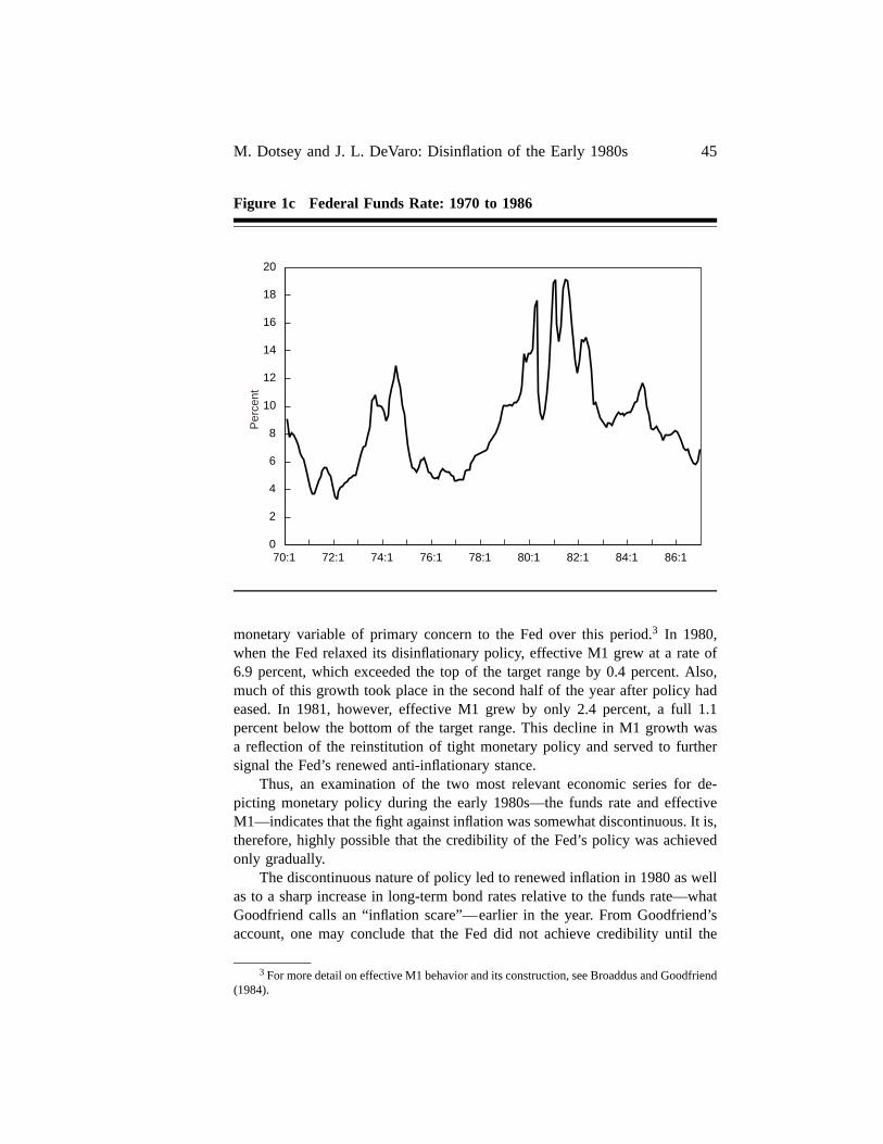
M. Dotsey and J. L. DeVaro: Disinflation of the Early 1980s 45
Figure 1c Federal Funds Rate: 1970 to 1986
70:1 72:1 74:1 76:1 78:1 80:1 82:1 84:1 86:10
2
4
6
8
10
12
14
16
18
20P
erce
nt
+
monetary variable of primary concern to the Fed over this period.3 In 1980,when the Fed relaxed its disinflationary policy, effective M1 grew at a rate of6.9 percent, which exceeded the top of the target range by 0.4 percent. Also,much of this growth took place in the second half of the year after policy hadeased. In 1981, however, effective M1 grew by only 2.4 percent, a full 1.1percent below the bottom of the target range. This decline in M1 growth wasa reflection of the reinstitution of tight monetary policy and served to furthersignal the Fed’s renewed anti-inflationary stance.
Thus, an examination of the two most relevant economic series for de-picting monetary policy during the early 1980s—the funds rate and effectiveM1—indicates that the fight against inflation was somewhat discontinuous. It is,therefore, highly possible that the credibility of the Fed’s policy was achievedonly gradually.
The discontinuous nature of policy led to renewed inflation in 1980 as wellas to a sharp increase in long-term bond rates relative to the funds rate—whatGoodfriend calls an “inflation scare”—earlier in the year. From Goodfriend’saccount, one may conclude that the Fed did not achieve credibility until the
3 For more detail on effective M1 behavior and its construction, see Broaddus and Goodfriend(1984).
46 Federal Reserve Bank of Richmond Economic Quarterly
summer of 1982. It is thus entirely possible that although the Fed announcedits resolve to fight inflation as early as October 1979, the policy was not fullycredible until mid-1982. Thus, it may be that much of the disinflation was unex-pected and that the 1980-83 period is perfectly consistent with the neoclassicalmodel.
To shed further light on the degree to which the disinflation was antici-pated, we adopt the innovative empirical methodology of Hamilton (1992). Bycombining information in commodity futures markets with the macroeconomicinformation readily available at the time, we decompose actual inflation into itsanticipated and unanticipated components. Our results imply that a substantialportion of the disinflation was unanticipated and that the Fed suffered from acredibility problem.
2. METHODOLOGY4
To analyze the degree to which the disinflation of the early 1980s was an-ticipated, we must construct a series depicting the public’s expectations ofinflation. The methodology we use for constructing such a series is that ofHamilton (1992). His procedure incorporates publicly available aggregate dataand financial market data on commodity futures contracts to estimate price-levelexpectations. The data on futures contracts are optimally weighted in an effortto uncover information possessed by the public but not by the econometrician.The use of future changes in commodity prices from their expected valuesrepresents a novel way to uncover what agents believed at any given moment.Because the change in policy was a major one, these data are potentially use-ful for uncovering beliefs about inflation since financial markets often reactaggressively to changing inflationary expectations.5
Specifically, suppose that the public’s expectation of next period’s pricelevel, pt+1, is given by
pet+1 = x′tδ + αt, (1)
where the superscript e denotes an expectation, xt is a vector of all relevantaggregate information, and αt represents information that agents find valuablein forecasting prices but that is unavailable to the econometrician. For example,xt could include economic time series published by the Commerce Departmentor the Federal Reserve, while αt could involve disaggregated information thatindividuals observe but that is unpublished.
4 The description in this section draws heavily on Hamilton (1992), who provides a moredetailed and technically rigorous description.
5 The model does not explicitly incorporate regime changes and to some extent suffers fromthe same problems as a standard VAR when regimes actually do change.

M. Dotsey and J. L. DeVaro: Disinflation of the Early 1980s 47
Let the public’s true expectational error be defined by at+1 ≡ pt+1 − pet+1.
Note that under rational expectations at+1 is white noise and uncorrelated withtime t information. Next, consider the forecasting error, ut+1, that occurs fromthe prediction of pt+1 using only the information in xt. Specifically, ut+1 is theerror term in
pt+1 = x′tδ + ut+1, (2)
which is a typical forecasting equation. From equation (1) and the definitionof at+1, ut+1 is equal to αt + at+1. By including enough own lags of pt in xt,ut+1 can be made white noise. A simple and consistent assumption is to treatαt as white noise as well.
Because the variance of ut+1, σ2u is equal to σ2
α+σ2a , we observe that if the
econometrician uses only the information in xt to forecast pt+1, the varianceof the forecast errors will exceed that of the true forecast errors. Improvingupon these forecasts requires inferences of αt. The better the inference of αt thecloser the econometrician’s forecast will coincide with the public’s. Hamiltonproposes that data from commodities markets be used to help form an optimalprediction of αt.
For ease of exposition, we will analyze the case in which there is onecommodity. Using data on the log of the commodity’s forward price at date t,ft, and the log of its expected future spot price next period, Etst+1, a simpleefficient markets model implies that
ft = Etst+1 − k, (3)
where k incorporates the variance of st and a constant risk premium. Equation(3) implies that the forecast error of the spot price is observable and given by
st+1 − ft = k + vt+1, (4)
where vt+1 is the forecast error. Under rational expectations, vt+1 is uncorre-lated with time t information. In particular, it is uncorrelated with the elementsof xt and αt. It is reasonable, however, to believe that the forecast error fora given commodity and the aggregate price level are correlated. For example,any demand shock (such as a monetary policy shock) could influence all prices,including commodity prices, in a similar way. This relationship is given by
vt+1 = qaat+1 + et+1. (5)
Hence, observation of vt+1 implies some knowledge of at+1.Next, consider a regression of the forward price on information available
to the econometrician,
ft = x′tβ + ωt. (6)
In this regression, ωt represents information that agents find relevant for pric-ing a commodity and that is unavailable to the econometrician, because ft is

48 Federal Reserve Bank of Richmond Economic Quarterly
observed at time t, and if the econometrician had all the relevant informationthen ωt would be zero. Thus, ωt has an interpretation similar to αt, and the twoshould be related. Let this relationship be described by the linear projection
ωt = qααt + εt, (7)
where εt denotes information that agents have about future commodity pricemovements that is uncorrelated with aggregate price movements.
The statistical problem is to form an optimal forecast of αt given knowledgeof ut+1, vt+1, and ωt, because it is these three observed disturbances that containinformation about αt. This optimal forecast allows us to form the expectationof the aggregate price level that best represents the one formed by the public.Using data on aggregate prices, commodity spot and forward prices, and xt,construct the error terms ut+1, vt+1, and ωt according to equations (2), (4), and(6). The optimal predictor of αt can then be formulated as
Et+1αt = A1ut+1 + A2ωt + A3vt+1, (8)
whereA1
A2
A3
=
σ
2a + σ2
α qασ2α qaσ2
a
qασ2α (qα)2σ2
α + σ2ε 0
qaσ2a 0 (qa)2σ2
a + σ2e
−1 σ2
α
qασ2α
0
. (9)
The coefficients in equation (8) are population regression coefficients. The ma-trix in (9) is the variance-covariance matrix of the disturbances ut+1 = at+1+αt.In deriving this matrix, various orthogonality conditions implied by rationalexpectations were used. The vector [σ2
α, qασ2α, 0]′ is the covariance between
αt and the three observed disturbance terms.The optimal forecast of next period’s price level is then depicted by
pet+1 = x′tδ + A1(pt+1 − x′tδ) + A2(ft − x′tβ) + A3(st+1 − ft − k). (10)
In calculating the public’s expectations of next period’s price level, the econo-metrician uses time t + 1 information from commodity spot markets. Thisinformation is needed to extract the optimal forecast of αt, which containsrelevant information available to the public but not to the econometrician.
Unfortunately, there is one technical difficulty. To estimate the coefficientsA1, A2, and A3, we must have estimates of qa, qα, σ2
a , σ2α, σ2
e , and σ2ε. The
variance-covariance matrix in (9), however, has only five independent piecesof information, which means that the system is not identified. An additionalrestriction is needed, and we follow Hamilton by imposing qa = qα.6
6 The solution is A1 = (1/∆)[q2σ2ασ
2ε(σ2
a + σ2e )]
A2 = (1/∆)qσ2aσ
2ασ
2e
A3 = −(1/∆)qσ2aσ
2ασ
2ε and ∆ = (σ2
a + σ2α)σ2
eσ2ε + q2σ2
aσ2α(σ2
e + σ2ε).
M. Dotsey and J. L. DeVaro: Disinflation of the Early 1980s 49
This restriction has some intuitive appeal. Suppose, for example, that therelevant aggregate information that agents possess is a demand shock that af-fects commodity prices and the aggregate price level in similar ways. That is,anticipated and unanticipated movements affect st+1 and pt+1 proportionately,although the absolute effects of an anticipated movement need not be the sameas those of an unanticipated movement. Then qa and qα should be equal.Under the restriction qa = qα, the ratio of the covariance of ut+1 and vt+1 tothe covariance of ut+1 and ωt is equal to σ2
a /σ2α, which reflects the extent that
agents are actually surprised by movements in the aggregate price level.However, this restriction may not be valid. If, for example, the unantici-
pated disturbances that affect commodity prices are largely idiosyncratic, whilethe information that agents actually possess affects both markets similarly, thenqa would not equal qα. In any event, the restriction can be tested. And withmultiple commodities, the restriction need only be placed on one commodityto achieve identification.
3. ESTIMATIONBefore estimating the analogous multivariate system given by (1), (4), (6), andthe variance-covariance matrix in (9), we describe our commodity price dataand perform some necessary diagnostic tests. We used data on wheat, corn,oats, and soybean futures, since these were the only commodity data availablefor our sample period. In what follows, we use the price of a futures contractthat is about to expire as the measure of the spot price. Because the futurescontracts are four months in duration, the data set is three times per year (suchintervals are denoted by roman numerals).
Commodity Price Behavior
Expected and actual inflation rates for the four commodities are given inTable 1. Actual inflation in a commodity market is calculated as the change inthe log of the spot price during the period in question, while expected inflationis represented by three times the average log difference between the four-monthfutures price and the spot price at each four-month interval. From the table itis evident that expected commodity price increases greatly exceeded actualincreases during the 1981-83 period. Further, graphs of expected commodityprice inflation versus actual commodity price inflation (Figures 2a to 2d) showthat, with the exception of oats, expected inflation was generally higher thanactual inflation. These results foreshadow the main results of the statisticalmodel: the overestimate of commodity price inflation will be mirrored in anoverprediction of the aggregate inflation rate.
Commodity Market Efficiency
One of the maintained hypotheses of the model discussed in Section 2 is thatthe commodity market is efficient. This was depicted by equation (4) in which
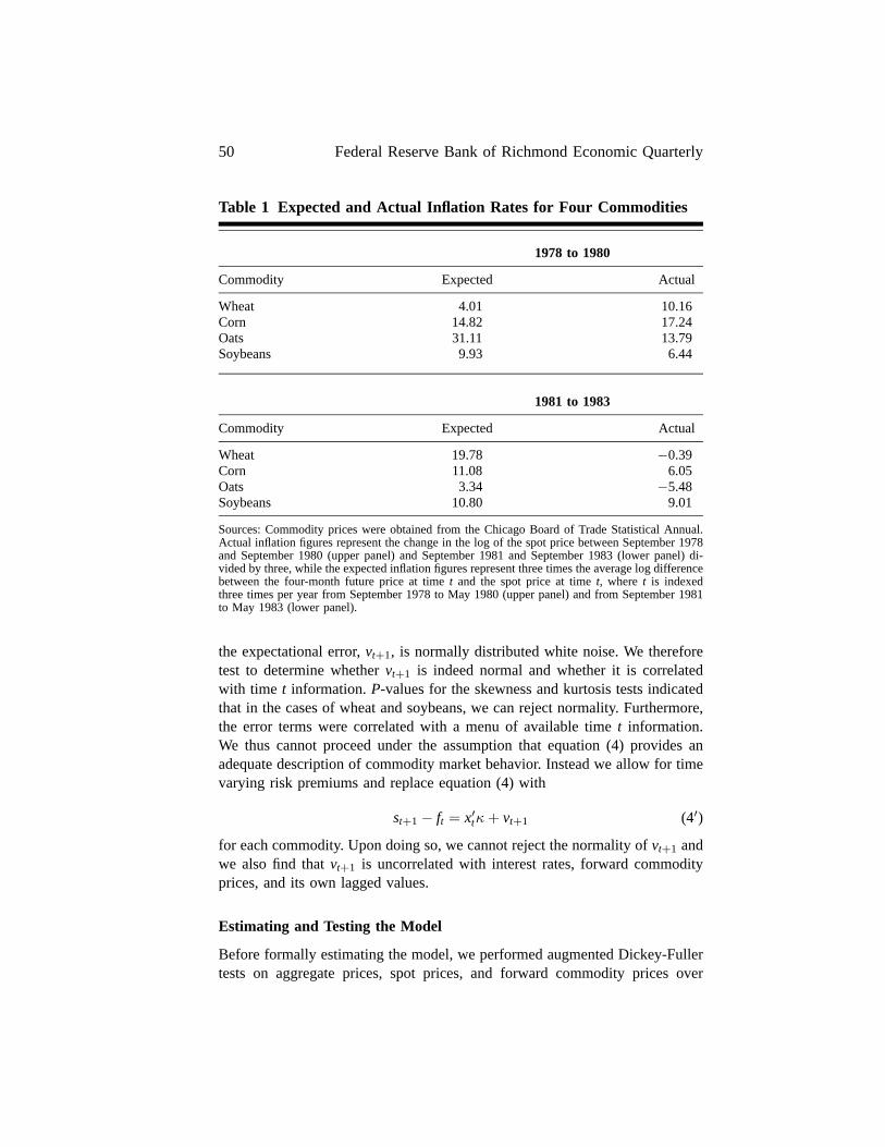
50 Federal Reserve Bank of Richmond Economic Quarterly
Table 1 Expected and Actual Inflation Rates for Four Commodities
1978 to 1980
Commodity Expected Actual
Wheat 4.01 10.16Corn 14.82 17.24Oats 31.11 13.79Soybeans 9.93 6.44
1981 to 1983
Commodity Expected Actual
Wheat 19.78 −0.39Corn 11.08 6.05Oats 3.34 −5.48Soybeans 10.80 9.01
Sources: Commodity prices were obtained from the Chicago Board of Trade Statistical Annual.Actual inflation figures represent the change in the log of the spot price between September 1978and September 1980 (upper panel) and September 1981 and September 1983 (lower panel) di-vided by three, while the expected inflation figures represent three times the average log differencebetween the four-month future price at time t and the spot price at time t, where t is indexedthree times per year from September 1978 to May 1980 (upper panel) and from September 1981to May 1983 (lower panel).
the expectational error, vt+1, is normally distributed white noise. We thereforetest to determine whether vt+1 is indeed normal and whether it is correlatedwith time t information. P-values for the skewness and kurtosis tests indicatedthat in the cases of wheat and soybeans, we can reject normality. Furthermore,the error terms were correlated with a menu of available time t information.We thus cannot proceed under the assumption that equation (4) provides anadequate description of commodity market behavior. Instead we allow for timevarying risk premiums and replace equation (4) with
st+1 − ft = x′tκ + vt+1 (4′)
for each commodity. Upon doing so, we cannot reject the normality of vt+1 andwe also find that vt+1 is uncorrelated with interest rates, forward commodityprices, and its own lagged values.
Estimating and Testing the Model
Before formally estimating the model, we performed augmented Dickey-Fullertests on aggregate prices, spot prices, and forward commodity prices over

M. Dotsey and J. L. DeVaro: Disinflation of the Early 1980s 51
Figure 2a Expected and Actual Commodity Price Inflation for Wheat:1970 to 1985
1970:III 1973:III 1976:III 1979:III 1982:III 1985:III-40
-20
0
20
40
60
80
Per
cent
Actual
Expected
+
Note: Roman numerals denote four-month intervals.
the period 1970:II to 1986:III. We could not reject nonstationarity of the pricelevel, but we were able to reject nonstationarity of commodity prices. Also, forut+1 to be white noise required the inclusion of two lags of the inflation rate.The system that we estimate is depicted by
∆pt+1
ftst+1 − ft
=
δ′
β′
κ′
xt +
ut+1
ωt
vt+1
, (11)
where f and s are 4 by 1 vectors, δ is a 9 by 1 coefficient vector, β and κare 9 by 4 matrices of coefficients, and u, ω, and v are the disturbance terms.The vector of explanatory variables xt includes a constant term, two seasonaldummies (d1 and d2), two lags of the inflation rate, and the four commodityspot prices.7
7 This is a fairly parsimonious statistical model. In principle, other variables such as incomeor money could be included, but doing so would greatly increase the computational burden. Ourrepresentation of the inflation process follows Hamilton (1992).

52 Federal Reserve Bank of Richmond Economic Quarterly
Figure 2b Expected and Actual Commodity Price Inflation for Corn:1970 to 1985
1970:III 1973:III 1976:III 1979:III 1982:III 1985:III-50
-40
-30
-20
-10
0
10
20
30
40
Per
cent
Actual
Expected
+
Note: Roman numerals denote four-month intervals.
The variance-covariance matrix in (9) is now 9 by 9 and is given by
Ω =
σ
2a + σ2
α
σ2α(qα)′
σ2a(qa)′
σ2α(qα)′
σ2αqα(qα)′ + Σ
0
σ2a(qa)′
0σ2
aqa(qa)′ + S
, (12)
where Σ = E[εtε′t] and S = E[ete′t]. We estimate equations (11) and (12)
by full-information maximum-likelihood and jointly test the orthogonalityconditions assumed under rational expectations and the identifying restrictionqα = qa. We use the Sims (1980) adjusted likelihood-ratio test, which is distrib-uted χ2(19).8 The p-value for the test statistic was 0.45, implying that we cannotjointly reject the restrictions at standard confidence levels. However, for thesystem using all four commodities, there is not significant covariation betweenωt and ut+1, and ωt and vt+1. As a result, we cannot reject the hypothesis thatqa = qα = 0.
This lack of rejection is due largely to the inclusion of wheat. Figure2a shows that actual wheat inflation is volatile, especially early in the sample
8 The test statistic is 2( T−kT ) (likelihood [unrestricted]-likelihood [restricted]).
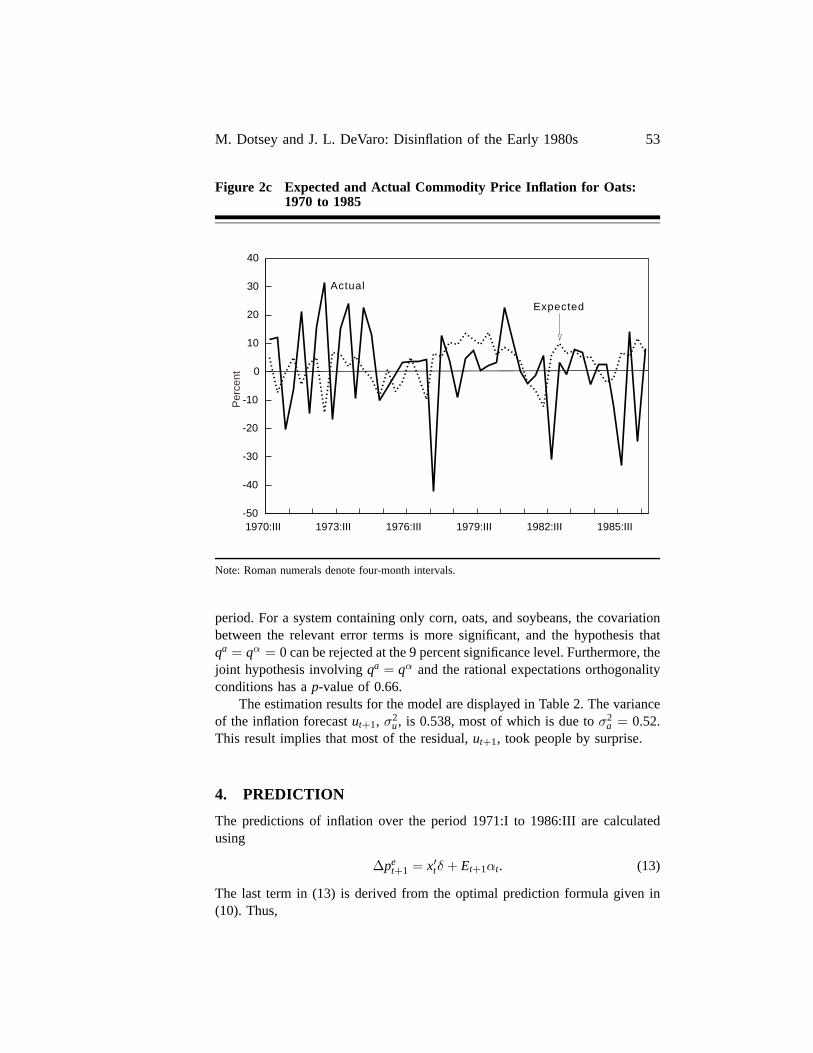
M. Dotsey and J. L. DeVaro: Disinflation of the Early 1980s 53
Figure 2c Expected and Actual Commodity Price Inflation for Oats:1970 to 1985
1970:III 1973:III 1976:III 1979:III 1982:III 1985:III-50
-40
-30
-20
-10
0
10
20
30
40
Per
cent
Actual
Expected
+
Note: Roman numerals denote four-month intervals.
period. For a system containing only corn, oats, and soybeans, the covariationbetween the relevant error terms is more significant, and the hypothesis thatqa = qα = 0 can be rejected at the 9 percent significance level. Furthermore, thejoint hypothesis involving qa = qα and the rational expectations orthogonalityconditions has a p-value of 0.66.
The estimation results for the model are displayed in Table 2. The varianceof the inflation forecast ut+1, σ2
u , is 0.538, most of which is due to σ2a = 0.52.
This result implies that most of the residual, ut+1, took people by surprise.
4. PREDICTION
The predictions of inflation over the period 1971:I to 1986:III are calculatedusing
∆pet+1 = x′tδ + Et+1αt. (13)
The last term in (13) is derived from the optimal prediction formula given in(10). Thus,

54 Federal Reserve Bank of Richmond Economic Quarterly
Figure 2d Expected and Actual Commodity Price Inflation for Soybeans:1970 to 1985
1970:III 1973:III 1976:III 1979:III 1982:III 1985:III-80
-60
-40
-20
0
20
40
60
Per
cent
Actual
Expected
+
Note: Roman numerals denote four-month intervals.
∆pet+1 = −1.76 − 0.08d1t − 0.08d2t + 0.35∆pt + 0.14∆pt−1 (14)
−0.006sc,t − 0.012so,t + 0.018ss,t
+0.0045(pt+1 − x′tδ)
−0.011(fc,t − x′tβc) − 0.012(fo,t − x′tβo)
+0.041(fs,t − x′tβs)
−0.000041(sc,t+1 − x′tκc) − 0.000027(so,t+1 − x′tκo)
−0.000013(ss,t+1 − x′tκs),
where the subscripts c, o, and s refer to corn, oats, and soybeans.Using (14) we can decompose the forecasts of inflation into simple fore-
casts, x′tδ, and the individual contributions from the price term (pt+1 − x′tδ),the three futures terms (ft − x′tβ), and the three commodity market surpriseterms (st+1 − ft − x′tκ). These decompositions are given in Table 3. Examiningthe entire sample period, the contributions of the price term and the futuresterm can at times be meaningful, affecting the forecasts by an annual rate ashigh as 87 and 51 basis points, respectively. The commodity market surprise

M. Dotsey and J. L. DeVaro: Disinflation of the Early 1980s 55
Table 2 Estimation Results+
unrestricted log likelihood : −760.43
restricted log likelihood : −765.55(qa = qα and orthogonality conditions imposed)
restricted log likelihood : −769.46(qa = qα = 0 and orthogonality conditions imposed)
σ2α = 0.017 σ2
a = 0.52 q ′ =
[4.60 2.59 23.41
(0.65) (0.60) (0.39)
]
Σ =
5.84 4.62 3.18
4.62 25.42 9.093.18 9.09 4.80
S =
171.08 72.26 45.97
72.26 123.17 − 69.9445.97 − 69.94 3712.3
Ω =
0.54 0.08 0.04 0.40 2.40 1.35 12.220.08 6.21 4.82 5.03 0 0 00.04 4.82 25.53 10.13 0 0 00.40 5.03 10.13 14.19 0 0 02.40 0 0 0 182.1 78.48 102.21.35 0 0 0 78.48 126.7 −38.3
12.22 0 0 0 102.2 − 38.3 39.98
+ Standard errors for the elements of q′ are in parentheses. The commodities are ordered corn,oats, and soybeans.
term, however, rarely has much effect on the forecasts, which is attributableto the small covariance between ut+1 and vt+1. Expectations of inflation aredisplayed in Table 4. The first two columns give the four-month actual andexpected inflation rates at annualized rates, the third and fourth columns giveeight-month actual and expected inflation at annualized rates, and the fifth andsixth columns give the annual actual and expected inflation rates. The firstexpectation reported in each instance is the one that is conditional on 1979:IIIinformation, since this is the period in which the Fed announced its disinfla-tionary objectives. For example, 13.78, the first number in column 6, is theinflation rate expected for 1980 given 1979:III information.
The eight-month-ahead and the one-year-ahead forecast errors strongly im-ply that a significant part of the disinflation in the early 1980s was unanticipated.Expected inflation exceeds actual inflation in all but three periods in the eight-month forecasts and in every period in the one-year forecast. On average, agents

56 Federal Reserve Bank of Richmond Economic Quarterly
Table 3 Decomposition of Expectation of Inflation
PeriodEnding Actual
SimpleForecast1
PriceTerm2
FuturesTerm3
SurpriseTerm4
1970:III 1.77 1.43 0.049 0.0005 0.0081971:I 1.00 1.38 −0.055 −0.028 0.0151971:II 1.23 1.56 −0.047 −0.072 0.0171971:III 0.98 1.54 −0.081 0.046 0.0021972:I 0.97 1.25 −0.040 0.033 0.0131972:II 1.19 1.58 −0.055 −0.11 −0.0061972:III 1.42 1.35 0.010 0.002 −0.0111973:I 2.77 1.44 0.19 0.17 −0.0061973:II 2.92 3.28 −0.052 −0.009 −0.0231973:III 3.48 3.29 0.027 −0.041 0.0101974:I 3.77 7.84 0.13 0.046 0.0041974:II 4.03 3.27 0.11 0.065 −0.0261974:III 3.30 3.53 −0.033 −0.012 0.0071975:I 1.52 3.15 −0.23 0.021 0.0131975:II 2.79 2.04 0.11 0.071 −0.0111975:III 2.17 1.70 0.068 −0.048 0.0081976:I 1.07 1.80 −0.10 −0.060 −0.0121976:II 2.11 1.27 0.12 −0.041 −0.0141976:III 1.89 1.58 0.04 0.023 0.0061977:I 2.52 2.11 0.060 0.049 −0.0101977:II 1.81 2.92 −0.16 −0.014 0.0321977:III 2.26 2.37 −0.016 −0.055 −0.0021978:I 2.83 2.16 0.10 0.075 −0.0081978:II 3.05 2.87 0.025 0.049 0.0151978:III 2.96 3.16 −0.028 −0.007 0.0121979:I 4.15 3.21 0.14 −0.047 −0.0001979:II 4.12 3.57 0.078 −0.066 0.0031979:III 4.73 3.91 0.12 0.072 0.0041980:I 4.63 3.94 0.10 −0.026 0.0011980:II 2.66 4.08 −0.20 −0.074 −0.0211980:III 3.86 3.36 0.072 0.009 0.0021981:I 2.83 2.73 0.013 0.005 −0.0031981:II 3.72 2.97 0.118 −0.067 0.0111981:III 1.39 2.64 −0.18 0.025 0.0091982:I 1.58 2.18 −0.086 −0.039 −0.0111982:II 1.86 1.27 0.084 −0.013 0.0141982:III 0.20 1.57 −0.20 0.080 0.0041983:I 1.32 1.11 0.030 −0.11 −0.0101983:II 1.20 0.89 0.044 −0.05 0.0211983:III 1.68 1.68 −0.001 −0.13 −0.0011984:I 1.36 1.55 −0.027 0.003 −0.0071984:II 1.15 1.74 −0.085 0.059 −0.0051984:III 0.95 1.10 −0.021 0.069 0.0011985:I 1.41 0.83 0.083 −0.066 −0.0061985:II .084 1.13 −0.042 0.099 0.0191985:III 1.65 1.34 0.045 0.036 −0.0071986:I −0.82 1.22 −0.29 −0.031 0.0161986:II 0.91 1.13 −0.031 0.11 0.0151986:III 1.35 0.49 0.12 −0.071 −0.019
1The simple forecast is equal to x′t δ.2The price term is given by A1(pt+1 − x′tδ) in equation (10).3The futures term is given by A2(ft − x′tβ) in equation (10).4The surprise term is given by A3(st+1 − ft − x′tκ).
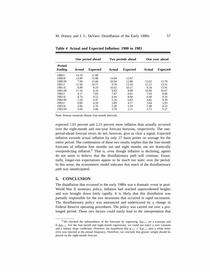
M. Dotsey and J. L. DeVaro: Disinflation of the Early 1980s 57
Table 4 Actual and Expected Inflation: 1980 to 1983
One period ahead Two periods ahead One year ahead
PeriodEnding Actual Expected Actual Expected Actual Expected
1980:I 14.19 11.881980:II 13.89 11.88 14.04 12.871980:III 7.98 12.66 10.94 12.80 12.02 13.781981:I 11.58 10.17 9.78 13.10 11.15 13.311981:II 8.49 8.19 10.02 10.17 9.34 13.911981:III 11.16 9.18 9.83 8.88 10.40 10.671982:I 4.17 7.83 7.67 8.81 7.93 8.901982:II 4.74 6.51 4.44 8.84 6.68 9.101982:III 5.58 4.47 5.16 6.03 4.82 9.291983:I 0.60 4.59 3.09 4.17 3.64 5.931983:II 3.96 2.76 2.28 5.03 3.38 4.231983:III 3.60 3.06 3.78 2.11 2.73 5.27
Note: Roman numerals denote four-month intervals.
expected 1.03 percent and 2.23 percent more inflation than actually occurredover the eight-month and one-year forecast horizons, respectively. The one-period-ahead forecast errors do not, however, give as clear a signal. Expectedinflation exceeds actual inflation by only 27 basis points on average for theentire period. The combination of these two results implies that the four-monthforecasts of inflation four months out and eight months out are drasticallyoverpredicting inflation.9 That is, even though inflation is declining, agentsdo not seem to believe that the disinflationary path will continue. Essen-tially, longer-run expectations appear to be much too static over the period.In this sense, the econometric model indicates that much of the disinflationarypath was unanticipated.
5. CONCLUSIONThe disinflation that occurred in the early 1980s was a dramatic event in post-World War II monetary policy. Inflation had reached unprecedented heightsand was brought down fairly rapidly. It is likely that this disinflation waspartially responsible for the two recessions that occurred in rapid succession.The disinflationary policy was announced and underscored by a change inFederal Reserve operating procedures. The policy was carried out over a pro-longed period. These two factors could easily lead to the interpretation that
9 We checked the unbiasedness of the forecasts by regressing ∆pt+1 on a constant andEt∆pt+1. For the four-month and eight-month regressions, we could not reject a zero constantand a unitary slope coefficient. However, the hypothesis that pt+1 = Etpt+1 plus a white noiseerror was rejected at the annual frequency. Therefore, we conclude that greater weight should beplaced on the eight-month forecast.

58 Federal Reserve Bank of Richmond Economic Quarterly
the disinflation was anticipated and, therefore, that this episode is consistentwith theories emphasizing the impact of anticipated monetary policy on realeconomic activity.
Although the policy was announced, evidence documented by Goodfriend(1992) suggests that it may not have been entirely credible. Hence the actualdisinflation could still have been unanticipated. Determining the extent to whichthe disinflation was unanticipated can help ascertain the degree to which Fedcredibility was lacking.
In an attempt to resolve whether the disinflation was anticipated, we per-formed a statistical analysis of the public’s expectations of inflation using themethodology developed in Hamilton (1992). Our conclusion is that much ofthe disinflation was unanticipated and that the Fed suffered from a credibilityproblem. The fact that much of the disinflation was unanticipated, however,does not allow us to discriminate among the competing models outlined inthe introduction. Such discrimination would necessarily involve a more subtlehypothesis test.
REFERENCES
Akerlof, George A., Andrew Rose, and Janet Yellen. “Comments andDiscussion,” Brookings Papers on Economic Activity, 1:1988, pp. 66-75.
Ball, Lawrence. “What Determines the Sacrifice Ratio?” Working Paper No.4306. Cambridge: National Bureau of Economic Research, March 1993.
, N. Gregory Mankiw, and David Romer. “The New KeynesianEconomics and the Output-Inflation Trade Off,” Brookings Papers onEconomic Activity, 1:1988, pp. 1-65.
Broaddus, J. Alfred, and Marvin Goodfriend. “Base Drift and the Longer-RunGrowth of M1: Experience from a Decade of Monetary Targeting,”Federal Reserve Bank of Richmond Economic Review, vol. 70 (Novem-ber/December 1984), pp. 3-14.
Fischer, Stanley. “Contracts, Credibility, and Disinflation,” in John W. Nevilleand Victor E. Argy, eds., Inflation and Unemployment: Theory, Experience,and Policymaking. Boston: Allen and Unwin, 1985.
. “Wage Indexation and Disinflation,” in Stabilization of theDomestic and International Economy. Carnegie-Rochester ConferenceSeries on Public Policy, vol. 5 (1977), pp. 107-48.
Goodfriend, Marvin. “Interest Rate Policy and the Inflation Scare Problem:1979-1992,” Federal Reserve Bank of Richmond Annual Report (1992),pp. 7-19.

M. Dotsey and J. L. DeVaro: Disinflation of the Early 1980s 59
Hamilton, James D. “Was the Deflation during the Great Depression An-ticipated? Evidence from the Commodity Futures Market,” AmericanEconomic Review, vol. 82 (March 1992), pp. 157-78.
Lucas, Robert E. “Some International Evidence on Output-Inflation Tradeoffs,”American Economic Review, vol. 63 (June 1973), pp. 326-34.
McCallum, Bennett T. “Rational Expectations and Macroeconomic Stabiliza-tion Policy: An Overview,” Journal of Money, Credit, and Banking, vol.12 (November 1980), pp. 716-46.
Sargent, Thomas J., and Neil Wallace. “Rational Expectations, the OptimalMonetary Instrument, and the Optimal Money Supply Rule,” Journal ofPolitical Economy, vol. 83 (April 1975), pp. 241-54.
Sims, Christopher A. “Macroeconomics and Reality,” Econometrica, vol. 48(January 1980), pp. 1-48.
Taylor, John B. “Aggregate Dynamics and Staggered Contracts,” Journal ofPolitical Economy, vol. 88 (February 1980), pp. 1-23.

The Fair Lending Lawsand Their Enforcement
John R. Walter
J ournalists, businessmen, politicians, and regulators are paying increasingattention to the subject of discrimination in lending, with particular em-phasis on mortgage lending. It sometimes seems as though the main issues
in antidiscrimination efforts have shifted from education and labor markets tothe credit markets.
Two different federal laws deal with discrimination in lending: the FairHousing Act (FHAct) and the Equal Credit Opportunity Act (ECOA). Thesefair lending laws prohibit lenders from discriminating in credit transactionson the basis of race, color, national origin, religion, sex, and other specifiedgrounds.1 But the laws provide little practical guidance for enforcement, par-ticularly with regard to the role of the banking regulatory bodies. Congress leftto these agencies and to the courts the job of working out the specifics of howto define and promote the laws’ purpose—fair lending.
While discrimination has been discussed widely in the popular and profes-sional press, an overview of the two fair lending laws and their enforcementis difficult to find. Section 1 describes these laws, their origins, and the in-terpretations that the courts and enforcement agencies have given some of
This article has benefited greatly from comments and suggestions from Marvin Goodfriend,Tom Humphrey, Anatoli Kuprianov, Jeffrey Lacker, Roy Webb, and John Weinberg. AlexMendoza provided excellent research assistance. The views expressed herein are the author’sand do not represent the views of the Federal Reserve Bank of Richmond or the FederalReserve System.1 Two other laws often mentioned in discussions of fair lending are the Home Mortgage
Disclosure Act of 1975 (HMDA) and the Community Reinvestment Act of 1977 (CRA). Whileboth laws play a part in current fair lending enforcement, neither prohibits discriminatory lending,so neither is defined as a fair lending law. The HMDA requires depository institutions to reportdata that are frequently used in investigations and studies of lending discrimination. The CRArequires the banking agencies to consider a depository institution’s efforts to meet the needs ofits community when it applies to the banking agencies for permission to expand. As currentlyinterpreted by the agencies, this has meant that a bank’s fair lending performance is weighedwhen considering such an application. For discussions of the HMDA and the CRA, see Cannerand Smith (1991) and Lacker (1995), respectively.
Federal Reserve Bank of Richmond Economic Quarterly Volume 81/4 Fall 1995 61

62 Federal Reserve Bank of Richmond Economic Quarterly
their provisions. Section 2 discusses the three major methods of enforcementof the laws: (1) complaints from aggrieved parties leading to investigationsby enforcement agencies, (2) civil court actions, and (3) examination by thefederal banking agencies.2 When it comes to their part of enforcing the fairlending laws, the banking agencies follow procedures long used in carrying outtheir responsibilities for bank safety and soundness. Specifically, they employperiodic fair lending examinations of all banks.3 Yet the examination of everyinstitution, whether or not the agency suspects discrimination, is strikinglydifferent from the practices of the federal agencies responsible for other areasof anti-discrimination law enforcement. Section 3 discusses the enforcement ofother antidiscrimination laws. The absence of periodic exams in other areas ofantidiscrimination law enforcement naturally leads one to ask whether routineuse of exams for banks is the most efficient means of enforcing the fair lend-ing laws. The concluding section raises briefly some issues that bear on thisquestion.
1. THE FAIR LENDING LAWS
The Fair Housing Act (FHAct) was passed as part of the Civil Rights Act of1968, which Congress enacted following urban unrest in many U.S. cities in1965, 1966, 1967, and after Rev. Martin Luther King, Jr.’s assassination in early1968. According to a Supreme Court opinion, Congress intended the FHActto contribute to the elimination of ghettos by reducing discriminatory housingpractices (Trafficante v. Metropolitan Life Insurance Company, 409 U.S. 205[1972], cited in Board of Governors, Consumer Compliance Handbook [1995]).
The FHAct prohibits discrimination in many activities of the residential realestate industry besides lending. The act prohibits discrimination by race, color,religion, sex, handicap, familial status (if a household includes children), andnational origin.4,5 It prohibits the refusal to sell, rent, or negotiate for the sale orrental of housing for discriminatory reasons. Varying the terms of sale or rentalin a discriminatory manner is prohibited, as is falsely claiming that housing isnot available for inspection, sale, or rental. The act also prohibits real estate
2 These agencies are the Federal Deposit Insurance Corporation, the Federal Reserve, theOffice of the Comptroller of the Currency, the Office of Thrift Supervision, and the NationalCredit Union Administration.
3 I will use the term “banks” throughout to refer to commercial banks, thrifts, and creditunions.
4 As passed, the FHAct prohibited discrimination on the basis of race, color, religion, andnational origin. A 1974 amendment added sex as a basis. A 1988 amendment added handicapand familial status.
5 Unless otherwise noted, I will use the word “discrimination” throughout to mean discrim-inating on the basis of categories such as race, gender, or familial status.

J. R. Walter: Fair Lending Laws and Their Enforcement 63
brokerage organizations, such as multiple-listing services, from discriminatingin their terms of access to the organization.
Section 805, the fair lending portion of the FHAct, makes discriminationunlawful in several aspects of home finance. Specifically, it prohibits discrim-ination in the making or purchasing of loans, the proceeds of which are forpurchasing, constructing, improving, repairing, or maintaining a dwelling. Theprohibition applies to any person or entity whose business includes engagingin residential real estate-related credit transactions.
The FHAct is enforced by the Department of Housing and Urban Devel-opment (HUD), by individuals, and by the Justice Department. Under the act,HUD may take enforcement actions against lenders based on complaints fromindividuals or on its own initiative. Individuals, or organizations representingindividuals, may pursue civil court actions under the act for discriminationagainst them. A civil action may be brought in a federal court by the Jus-tice Department whenever it believes that a lender is engaged in a pattern ofdiscrimination.
The federal bank regulatory agencies also enforce the act. These agenciesare the Federal Deposit Insurance Corporation (FDIC), the Federal Reserve(Fed), the Office of the Comptroller of the Currency (OCC), the Office of ThriftSupervision (OTS), and the National Credit Union Administration (NCUA).Since the act says little about their enforcement responsibilities, the bankingagencies have been left to determine largely on their own how to enforce theFHAct.
The fair lending section of the FHAct does not specify actions or policiesthat are considered discrimination.6 This means that the agencies responsiblefor the act’s enforcement have little to guide them in the investigation of lend-ing discrimination. At first blush, the identification of lending discriminationmight seem a simple matter. The difficulty arises because discrimination, in thebroad sense of the word, is a fundamental function of a successful lender. Toremain profitable, a lender must avoid (discriminate against) borrowers who areunlikely to repay, and favor those who will repay. Enforcement agencies areleft with the difficult job of separating appropriate discrimination from discrim-ination prohibited by the act. Court decisions have provided broad guidance,but detailed direction is lacking.
In 1972, a U.S. Supreme Court ruling established a procedure for deter-mining whether an individual has been treated differently based on his minoritystatus. Such discrimination goes by the phrase “disparate treatment.” The casedealt with employment discrimination, but the courts later applied the precedentto lending discrimination. The Supreme Court set out four factors that a plaintiff
6 This contrasts with the housing section of the FHAct, which provides an explicit list ofactions which are discriminatory under the law.

64 Federal Reserve Bank of Richmond Economic Quarterly
must establish to make a prima facie case of employment discrimination. Theplaintiff must show (1) that he belongs to a racial minority, (2) that he appliedand was qualified for a job for which the employer was seeking applicants, (3)that, despite his qualifications, he was rejected, and (4) that, after his rejection,the position remained open and the employer continued to seek equivalentlyqualified applicants (McDonnell-Douglas Corp. v. Green, 411 U.S. 792 [1973],cited in Board of Governors, Consumer Compliance Handbook [1995]).
To translate these standards for use in lending cases, the courts simplysubstituted the idea of creditworthiness qualifications for job qualifications(Hickson v. Home Federal of Atlanta, 805 F. Supp. 1567 [N.D. Ga., 1992];aff’d, 14 F.3d 59 [11th Cir. 1994], Gross v. U.S. Small Business Admin., 669F. Supp. 50 [N.D. N.Y., 1987]). Therefore, to make a prima facie case, theplaintiff must show (1) that he is a member of a protected class, (2) that heattempted to get a loan and met all relevant qualifications for doing so, (3)that the bank refused to make the loan despite the plaintiff’s qualifications, and(4) that, after his rejection, the bank continued to make loans to equivalentlyqualified applicants. Banking agency investigation procedures are based in parton determining whether these factors are met (see Board of Governors, Con-sumer Compliance Handbook [1995], p. 1.19). The courts and the agencies areleft to make difficult decisions, however. No two loan applications are exactlyalike, so it is impossible to match a rejected minority application perfectly to anaccepted non-minority application, and by doing so show discrimination. Thecourts and agencies must decide whether similar applications are enough likethe rejected minority application to persuasively show discrimination. At thevery least, however, this ruling provided what the statute lacked—a doctrine toguide policy.
In addition, courts and banking agencies have recognized that the FHAct’sprohibitions against discrimination extend to “redlining” (Laufman v. OakleyBuilding and Loan Co., 408 F. Supp. 489 [S.D. Ohio, 1976]; Ring v. First In-terstate Mortgage, Inc., 984 F.2d 924 [8th Cir. 1993]; Cloud and Galster 1993,p. 109; Board of Governors, Consumer Compliance Handbook [1995], p. 1.59).Redlining is the practice of denying loans for housing in certain neighborhoods,even if the loan applicants are creditworthy. According to the courts and bank-ing agencies, redlining is unlawful when the decision to avoid making loansin a particular neighborhood is based on the race, national origin, religion, orother similar categorization of residents of the neighborhood. Redlining is notunlawful when based entirely on economic considerations, such as the locationof a neighborhood in a flood plain (Interagency Task Force on Fair Lending[1994], p. 5; Board of Governors, Consumer Compliance Handbook [1995],pp. 1.58–1.59).
The Equal Credit Opportunity Act also prohibits lending discrimination.This act was passed in 1974 as an amendment to the much broader Consumer
J. R. Walter: Fair Lending Laws and Their Enforcement 65
Credit Protection Act, passed in 1968.7 Specifically, the ECOA prohibits dis-crimination in all personal and commercial credit transactions based on race,color, religion, national origin, sex, marital status, age, and other bases.8 Theprohibitions apply to anyone regularly extending credit or arranging for theextension of credit. The ECOA is broader than the FHAct since the ECOAcovers virtually all lenders while the FHAct covers only real estate-relatedlending. Housing lenders are subject to both statutes.
As originally passed in 1974, the ECOA only prohibited discriminationbased on sex and marital status. Congressional hearings preceding the passageof the ECOA had produced testimony of lending discrimination against womenand particularly of women denied credit without the signature of a male (SenateRep. No. 589, 94th Cong., 2d Sess. 2, reprinted in U.S. Code: Congressionaland Administrative News 403, 404 [1976]; Board of Governors, ConsumerCompliance Handbook [1995], p. 1.12). Additional bases were added by a1976 amendment. In 1974 hearings, instances were reported of discriminationbased on age and race. In addition, during 1974 the banking agencies conductedstudies on loan acceptance and rejection rates for minority versus non-minorityapplicants. Holding creditworthiness factors constant, the studies found muchhigher rejection rates for minorities (Senate Rep. No. 589, 94th Cong., 2d Sess.2, reprinted in U.S. Code: Congressional and Administrative News 403, 405[1976]; U.S. Congress, Senate [1993], pp. 570–71).
Besides prohibiting lending discrimination, the ECOA includes some re-quirements not explicitly related to fair lending. Within thirty days of anapplication, a lender must notify the loan applicant whether the applicationhas been accepted or rejected. In the case of a rejected application, a lendermust state the reasons for the denial or tell the denied applicant that he mayhave a statement of the reasons on request. Lenders also must provide, eitherroutinely or at the applicant’s request, copies of any appraisal reports.
The ECOA requires the banking agencies to ensure that depository insti-tutions comply with the act’s requirements. The ECOA delegates to the Fedthe authority to “prescribe regulations to carry out the purposes of the title.”These regulations are the Fed’s Regulation B. Each regulatory agency is re-sponsible for ensuring that the depository institutions it normally supervisescomply with the ECOA and Regulation B. Several other federal agencies areresponsible for enforcing compliance by other types of firms that make loans.
7 The Consumer Credit Protection Act encompasses the Truth in Lending Act, the Fair CreditReporting Act, the Equal Credit Opportunity Act, the Fair Debt Collection Practices Act, and theElectronic Fund Transfer Act.
8 Other bases on which lenders may not discriminate include an applicant’s status as arecipient of public assistance and an applicant’s claim of any right under the Consumer CreditProtection Act.

66 Federal Reserve Bank of Richmond Economic Quarterly
These agencies include the Federal Trade Commission, the Small BusinessAdministration, the Farm Credit Administration, and others.
The ECOA has left the agencies and the courts with much to work outconcerning its enforcement. For instance, like the FHAct, the ECOA leaveslargely undefined the actions and policies that are considered discrimination. Inaddition, the act does not tell the enforcement agencies how to uncover discrim-inating creditors or discriminating actions. While the FHAct outlines HUD’scomplaint response procedures, the ECOA does not address such procedures.
Nevertheless, like the FHAct, the ECOA stipulates that any creditor issubject to one of three enforcement actions. First, a person alleging injury maysue the creditor in a federal district court. Second, the federal agency withjurisdiction may take action against the creditor. Third, the Justice Departmentmay pursue a civil action against a suspected violator. Such action may occurif another enforcement agency refers the case to the Justice Department or ifthe Justice Department suspects a pattern of violations.
Court decisions have helped to define discrimination under the ECOA asthey have under the FHAct. In the legislative history of the 1976 amend-ment to the ECOA, Congress showed that it meant for the act to encompassa new concept of lending discrimination. Discrimination is to include not onlydisparate treatment (discussed above) but a discrimination standard recentlydeveloped by the courts, “disparate impact” (Senate Rep. No. 589, 94th Cong.,2d Sess. 2, reprinted in U.S. Code: Congressional and Administrative News403, 406 [1976]). Disparate treatment occurs when individuals receive differ-ent treatment because of their minority status. Disparate impact occurs whenminority individuals and non-minority individuals receive equivalent treatmentbut a lending policy has a disparate effect on minorities. Making loans foramounts no smaller than a set minimum is the classic example of a policy witha disparate impact. Since, on average, minorities are over-represented in lowincome brackets, they will more frequently seek low value loans. Therefore,they will be rejected more frequently for loans than will non-minorities undera minimum-loan-amount policy.
The courts developed the disparate impact standard in employment dis-crimination cases, including a 1971 Supreme Court ruling, Griggs v. DukePower Co. (401 U.S. 424 [1971]). In that case, several black employees ofDuke Power Company challenged as discriminatory the company’s policy ofrequiring a high school diploma and a passing score on an intelligence test asa prerequisite for hiring and promotion. The Court ruled that the Civil RightsAct of 1964 outlawed practices that had the effect of discriminating and thatDuke’s prerequisites had such an effect and were not significantly related toperformance of the jobs in question (Board of Governors [1977b], p. 106;Griggs v. Duke Power Co. (401 U.S. 424 [1971]).
Following the 1976 amendment to the ECOA, courts extended this rule tolending discrimination. They ruled that a complainant can make a prima facie
J. R. Walter: Fair Lending Laws and Their Enforcement 67
case of illegal lending discrimination if he can show that a lender’s policy hasa disproportionately adverse effect on a protected class. A policy is said to failthe so-called “effects test” if it has a disproportionately adverse effect (Cherryv. Amoco Oil Co., 490 F. Supp. 1026 [N.D. Ga., 1980]).
Various courts have come to different conclusions over the burden of proofthe lender must carry to rebut the complainant’s prima facie disparate impactcase. Some courts have ruled that a lender must show a “legitimate businessreason” for a practice that produces the disparate impact. Other courts haveruled that the lender must show a “business necessity,” a more stringent stan-dard. In 1994 the federal agencies enforcing the fair lending laws came outin favor of requiring the more strict burden for the lender (Interagency TaskForce on Fair Lending [1994], p. 7).9
2. ENFORCEMENT OF THE FAIR LENDING LAWS
There are three methods of enforcing the fair lending laws. First, the enforce-ment agencies may take action in response to complaints. Second, individualsor the Justice Department may bring civil court actions. Third, the bankingagencies periodically examine every bank for evidence of discrimination. Theagencies take remedial or punitive action if evidence of discrimination is found.
Complaints
An individual who believes he has suffered prohibited credit discriminationmay complain to (1) the Justice Department, (2) HUD if the loan is for realestate, or (3) the federal agency with fair lending enforcement powers over theinstitution believed to have discriminated. The FHAct requires HUD to receiveand respond to complaints of fair lending violations. The FDIC, the Fed, andthe OCC are each required to maintain a consumer affairs division by theMagnuson-Moss Warranty—Federal Trade Commission Improvement Act of1975 (U.S. Congress, Senate [1976], p. 1).10 These divisions receive and takeaction upon consumer complaints, such as complaints of fair lending violations.The Justice Department also responds to lending discrimination complaints thatit receives.
Each year these organizations together receive over a thousand complaintsof alleged credit discrimination (see U.S. Congress, Senate [1993], pp. 668–69,
9 For further discussion of the history and current status of the disparate impact standardin lending discrimination, see Vartanian, Ledig, and Babitz (1995), Dennis and Bachman (1995),and Board of Governors of the Federal Reserve System, Official Staff Commentary on RegulationB, Equal Credit Opportunity (1995), sect. 202.6(a)-2.
10 The name of the act derives from its sponsors Senator Warren G. Magnuson and Repre-sentative John E. Moss.
68 Federal Reserve Bank of Richmond Economic Quarterly
680, 700, and 742; U.S. Department of Justice, annual reports of the AttorneyGeneral [1977–1987]; U.S. Congress, Senate [1990], p. 119). The agenciesinvestigate each complaint of suspected lending discrimination. If the agenciesuncover evidence of discrimination, they may attempt to resolve the complaintby obtaining agreement between the parties. Beyond this, the banking agenciesand HUD may require remedial action or may penalize the violator, while theJustice Department can sue. Sometimes one agency refers the case to anotheragency.
Courts
Based on provisions in both the ECOA and the FHAct, an individual whobelieves he has suffered prohibited credit discrimination may also seek reliefdirectly from the courts. According to the legislative history of the ECOA,Congress viewed the power of individual claimants to bring civil court casesas a primary mode of enforcement of the statute (Senate Rep. No. 589, 94thCong., 2d Sess. 2, reprinted in U.S. Code: Congressional and AdministrativeNews 403, 415 [1976]).
Private fair housing and civil rights agencies have become more activein facilitating fair lending actions taken by individuals. For instance, one ofthe first agencies, the Toledo Fair Housing Center, has produced a number ofvictories for borrowers either in court, in settlements outside court, or throughcomplaints made to the federal enforcement agencies (Cloud and Galster 1993).Similar organizations also have become active recently, producing several largesettlements for their clients, and initiating additional suits (Sweet 1995, p. 4;Washington Post, September 22, 1995; American Banker, January 10, 1995).
Beyond the ability of individuals to bring court cases, the Justice De-partment may bring civil court actions under both the FHAct and the ECOA.Before 1988, Justice Department enforcement powers were limited under theFHAct and the ECOA; the Justice Department was not granted the powerto seek monetary awards. In 1988, an amendment to the FHAct granted theJustice Department the authority to seek monetary awards for damages andcivil penalties. A 1991 amendment to the ECOA similarly expanded the typesof relief the Justice Department could seek in fair lending cases brought underthat statute.
Before these amendments provided the Justice Department with the author-ity to seek monetary awards, most fair lending actions by the Justice Departmentresulted in small out-of-court settlements that aroused little popular interest.11
Since the early 1990s, however, every suit brought by the U.S. Department ofJustice has been the focus of great interest, at least among lenders. Each year
11 At least one lending discrimination case brought by the U.S. Justice Department went totrial (U.S. v. American Future Systems, Inc., 743 F.2d 169 [3d Cir. 1984]).
J. R. Walter: Fair Lending Laws and Their Enforcement 69
since 1992 the Justice Department has investigated several fair lending casesresulting in large out-of-court settlements against lenders. In these settlements,the lenders agreed to significant penalties, including compensation for victims,modification of lending procedures, and increased efforts to reach minorityindividuals or communities.
In civil court cases brought by individuals under the FHAct, the courtsmay award actual and punitive damages and other equitable relief. The act setsno maximum for these damage awards. In court cases brought by the JusticeDepartment under the FHAct, penalties for violations are the same as in casesbrought by individuals, except that civil penalties beyond actual damages arelimited to $50,000 for the first violation and $100,000 for any subsequentviolations. Under the ECOA, individuals and the Justice Department may seekactual damages and the imposition of injunctions. An injunction is a court orderrequiring a party to do or refrain from doing a specified act. But lenders maynot be made to pay punitive damages to an aggrieved individual greater than$10,000. In class action suits, punitive damages are limited to the lesser of$500,000 or 1 percent of the lender’s net worth.
Examination
Examination by the banking agencies provides the third method of enforcingthe fair lending laws. The banking agencies probe the institutions they supervisefor evidence of lending discrimination in periodic, on-site fair lending exami-nations. For banks examined by the Fed, a fair lending examination occurs atleast every two years. The other agencies have differing schedules.
Fair lending examinations have their origin in, and are modeled after, banksafety and soundness examinations. In a safety and soundness examination,examiners from a federal banking agency investigate a bank’s riskiness andfinancial health. The agencies examine every bank periodically. The examina-tions include an on-site analysis of the bank’s management, its policies andprocedures, and its key financial factors. Additionally, examiners verify that abank is complying with banking laws and regulations. Because of this, exam-iners gained responsibility for verifying compliance with the fair lending lawswhen these laws were passed.
Besides the fair lending laws, a number of other banking consumer pro-tection laws, such as the Truth in Lending Act, the Fair Credit Reporting Act,and the Fair Credit Billing Act, were passed by Congress during the 1960sand early 1970s. Examiners gained responsibility for banks’ compliance withthese laws too. Between 1976 and 1980 the FDIC, the Fed, the OCC, and theNCUA established “consumer compliance” examinations separate from safetyand soundness examinations because performing both consumer law compli-ance and safety and soundness tasks within the same examination was too

70 Federal Reserve Bank of Richmond Economic Quarterly
burdensome.12 Examiners who specialize in consumer law compliance (compli-ance examiners) perform fair lending examinations. The consumer complianceexamination covers the fair lending laws and the other consumer protectionlaws. While separate from the soundness examination, the consumer compli-ance examination follows the model of periodic, on-site examinations used inthe soundness examination.13
In the fair lending portion of compliance examinations, the examiner checksfor evidence of disparate treatment, redlining, and disparate impact. The exam-ination for disparate treatment of minorities may proceed along several lines.Since the early 1990s, the banking agencies have been using statistical teststo aid them in their search for evidence of discrimination.14 Compliance ex-aminers may run statistical tests on the outcomes of a bank’s loan approvalprocess to decide if minority status is correlated with the frequency of denial,factors other than minority status held equal. When such a correlation is found,examiners manually review a sample of loan application files to determinewhether factors omitted by the statistical testing methods explain the statisticalresults. The main focus of statistical testing is mortgage lending, since minoritystatus data are available only for mortgage loans.
Relatively large numbers of mortgage applications from both minoritiesand non-minorities are necessary for valid testing. Without large numbers, thetests cannot produce meaningful results. Only one in ten banks receives enoughmortgage loan applications to allow the use of these tests.15 Since these bankstend to be the largest mortgage lenders, large portions of all outstanding mort-gage loans are therefore made by banks subject to statistical testing.16
12 In January 1989, separate consumer compliance examinations for savings institutions wereestablished by the Federal Home Loan Bank Board (U.S. Congress, Senate [1990], pp. 36–37;U.S. Congress, Senate [1993], p. 693). In late 1989, Congress created the OTS to replace theFederal Home Loan Bank Board as supervisor of savings institutions, following the thrift crisisof the 1980s. The OTS continued the practice of separate consumer compliance examinations.
13 See Board of Governors (1977a) for a discussion of the history of consumer complianceexamination.
14 In the late 1970s and early 1980s, two of the banking agencies began using functionallysimilar but less sophisticated tests. The OCC and the FDIC collected data from banks they super-vised regarding loans accepted and rejected, race, income, and measures of creditworthiness ofthe applicant. They then ran statistical analyses that tested for correlations between minority statusand rejection, with creditworthiness held equal. The results of these tests guided examiner effortsin searching for evidence of discrimination. While the statistical testing procedures begun in the1990s are more sophisticated and employ more creditworthiness variables, the methodology andgoals are equivalent. The FDIC dropped its use of this technique in 1982 (U.S. Congress, Senate[1990], pp. 44, 155, and 170–71). For discussion of these early techniques, see U.S. GeneralAccounting Office (1981), pp. 50 and 84, and Milroy (1980), pp. 17–33, and 128.
15 Calem and Canner (1995), p. 121.16 For discussions of fair lending testing techniques, see Calem and Canner (1995), Bauer
and Cromwell (1994), and Stengel and Glennon (1995).
J. R. Walter: Fair Lending Laws and Their Enforcement 71
Examiners use only informal techniques when examining most banks, sinceformal statistical tests can be used only on a small portion of banks. Fair lend-ing examinations have included informal techniques since the late 1970s. Theexaminer typically chooses a sample of accepted and rejected applicants andgathers key creditworthiness information for the applicants from the bank’s loanapplication files. The examiner secures a written copy of the bank’s lendingdecision criteria or interviews bank officials to learn the criteria. For example,lending decision criteria might include the bank’s minimum down paymentpercentage, its maximum loan-to-value ratio, and its maximum debt-payments-to-income ratio. The examiner determines whether treatment of accepted andrejected applicants accords with the bank’s written or articulated loan criteria. Ifthe bank rejects minorities when its loan criteria suggest acceptance, or acceptsnon-minorities when the loan criteria suggest rejection, the examiner has reasonto suspect discrimination. The examiner will then expand his investigation. Forexample, assume a bank has a policy of normally rejecting applicants whosedebt-payments-to-income ratio will exceed 36 percent if granted the loan. Theexaminer might become suspicious if this bank allows higher ratios more fre-quently for whites than for Hispanics. Characteristics of sampled rejected andaccepted applicants are also compared directly to determine if the bank acceptsnon-minority applicants but rejects similarly qualified minority applicants. Ifthis comparison leads the examiner to suspect disparate treatment, he conductsa more intensive investigation.
In searching for signs of disparate treatment by a bank, the examiner alsocompares the racial and ethnic makeup of the bank’s application and loan poolsto the racial and ethnic makeup of its market area. If the proportion of appli-cations from minorities differs significantly from the proportion in the bank’smarket area, the examiner might suspect that the bank is discouraging minoritiesfrom applying for loans (“prescreening” minority applicants). Alternatively, asignificant differential between the proportion of minority loan approvals andthe proportion of minorities in the bank’s market area could be a sign that thebank is rejecting minorities for discriminatory reasons. In either case, furtherinvestigation would be called for (Board of Governors, Consumer ComplianceHandbook [1995], pp. 1.43–1.48).
Next, the examiner reviews the bank’s loan policies for any that couldamount to redlining or for any discriminatory impact. If the examiner findspolicies he believes may have such effects, the bank is allowed to present anexplanation.
The agencies’ responses to violations uncovered during examinations canvary. They may simply require the bank to change its loan policy. They may gofurther and require it to pay a sizeable monetary penalty either as restitution toinjured parties or to the U.S. Treasury. More serious or repeated violations canearn more severe penalties. Whenever an examination uncovers a pattern of fairlending violations, a provision of the ECOA requires the agencies to notify the

72 Federal Reserve Bank of Richmond Economic Quarterly
Justice Department.17 While the requirement applies explicitly only to ECOAviolations, it covers most FHAct violations as well. Most fair lending violationsof the FHAct will be violations of the ECOA, since the former act includesonly real estate lending, while the latter covers all types of lending. SomeFHAct violations will not be ECOA violations because protected classes differslightly under the two acts. Once notified, the Justice Department may thenchoose to investigate and bring a civil action. If the agencies find violations ofthe FHAct, they must report them either to HUD or to the Justice Department.
3. ENFORCEMENT OF OTHERANTIDISCRIMINATION LAWS
The first two sections of this article have discussed the fair lending laws andtheir enforcement. But these fair lending laws are only part of antidiscrim-ination law. For instance, laws also prohibit discrimination in employment,housing, and voting opportunities. This section contains a brief description ofthe enforcement activities of several major federal agencies responsible foremployment and housing antidiscrimination law. In contrast to the bankingagencies’ practice of examining all banks for evidence of credit discrimination,the federal employment and housing agencies do not employ routine examina-tions to enforce antidiscrimination statutes. Instead they investigate institutionsonly in response to a complaint or other signal of a possible violation. Alterna-tively, one employment-discrimination law-enforcement agency conducts audits(examinations) of a small subset of institutions. It also responds to complaints.
The major federal agency responsible for employment-discrimination lawenforcement investigates employers only if there is prior suspicion of discrim-inatory activity. The Equal Employment Opportunity Commission (EEOC) isresponsible for enforcing four laws prohibiting employment discrimination:the Civil Rights Act of 1964, the Equal Pay Act, the Age Discrimination inEmployment Act, and the Americans with Disabilities Act. The EEOC’s prin-cipal means of enforcing these statutes is through response to complaints ofdiscrimination. These complaints may come from an employee, a rejected jobapplicant, or an individual or organization acting on an employee’s behalf. TheEEOC handles complaints by investigating and making a determination on themerits of the complaint. It may seek a settlement between the parties. If theEEOC cannot produce a settlement, it may litigate the case (Bureau of NationalAffairs 1995, pp. 0:3101–0:3812).
Though complaints are the primary source of EEOC action, the EEOCmay itself initiate an investigation. Leads for these charges may come fromtips gathered during investigations of other employers. They also may come
17 This requirement was established by a 1991 amendment to the ECOA.

J. R. Walter: Fair Lending Laws and Their Enforcement 73
from the media, other government or private civil rights groups, union andtrade associations, and employment agencies. Data from employers on num-bers and classifications of minority and non-minority employees can provide alead (Bureau of National Affairs 1995, p. 8:0002).
Another leading federal employment discrimination enforcement agencyis the Office of Federal Contract Compliance Programs (OFCCP), a divisionof the Department of Labor. The OFCCP is responsible for the enforcementof three antidiscrimination and affirmative action statutes covering institutionsreceiving government contracts. It enforces the statutes with complaint inves-tigations and compliance reviews (“audits”), which are similar to the bankingagencies’ examinations.
Although the techniques used in an OFCCP audit are similar to thoseused in a bank fair lending examination, OFCCP audits only a small subset ofcontractors.18 For example, in 1994 it audited 4,100 contractors, selected froma population of 192,500, for compliance with the laws (Office of Federal Con-tract Compliance Programs [Undated]). Contractors are selected to be auditedbased in part on the percentage of women and minorities employed relativeto comparable percentages employed by the aggregate of all such employers(Fox 1993). Even if no problems are found, an audit is costly for the auditedcontractor.19 Therefore, the threat of an audit provides an incentive for con-tractors to maintain the percentage of women and minorities they employ ator above their peer group’s average. This helps the OFCCP meet its affirma-tive action responsibilities. Other factors are considered when deciding whichcontractor to audit. These factors are the time elapsed since the last audit,employee or job applicant complaints, negative community group comments,and whether the contractor is adding employees (Fox 1993). Unlike bank fairlending examinations, to which all banks are subject periodically, contractorsmay go years without an OFCCP audit, if they are audited at all.
The primary federal enforcement agency responsible for housing discrim-ination is HUD. Like the EEOC, HUD investigations typically result fromcomplaints of discrimination. Occasionally HUD initiates an investigation. Forexample, some sign of housing discrimination, such as a newspaper story, cangenerate this type of investigation.
18 During OFCCP audits, personnel files are examined to determine if comparable minorityand non-minority individuals are treated similarly. Personnel policies are examined for any poli-cies that may have a discriminatory effect. The treatment of minorities relative to policies areexamined for signs of discrimination.
19 According to Fox (1993), an audit costs a contractor an average of $25,000.
74 Federal Reserve Bank of Richmond Economic Quarterly
4. CONCLUDING COMMENT
Banking agencies enforce fair lending laws by examining all banks for evi-dence of discrimination. As we saw in Section 3, this contrasts sharply withenforcement in other areas of antidiscrimination law, where routine examina-tions are not employed. The banking agencies’ general use of routine examshas evolved as the best means of guaranteeing the safety and soundness ofthe banking system. But are routine examinations the most efficient means ofensuring fair lending? This is a difficult question.
The examination of every bank, whether or not it is suspected of discrim-ination, is expensive for both banking agencies and banks themselves. Relyinginstead on other enforcement mechanisms, such as complaints and legal actions,has the great advantage of directing scarce resources to identifiable problems.Nevertheless, one can imagine several issues that ought to be considered inweighing the costs and benefits of the alternatives. Victims of discriminatorylending practices may not always be aware of the discrimination. If this is thecase, then complaints and private lawsuits might not induce sufficient enforce-ment. On the other hand, enforcement agencies receive hundreds of complaintsof discrimination each year. Moreover, the growing interest of housing groups,the press, and attorneys in credit discrimination will expand borrowers’ knowl-edge of the laws that protect them and thus encourage complaints and lawsuits.
Matters are complicated further by the fact that fair lending legal actionsseem likely to produce benefits to society beyond those received by the plain-tiff alone. For example, policies of a defendant bank that are unknowinglydiscriminatory may be identified by a lawsuit, and eliminated as a result. Con-sequently, future customers will be less likely to be victims of discrimination.Since plaintiffs do not reap all the benefits of their own legal actions, the num-ber of court cases brought may be too low from society’s point of view. Onthis basis one might argue that routine examination of all banks, coupled withthe threat of penalties, supplements the antidiscrimination benefits provided bylawsuits. But an alternative to employing routine exams to supplement legalactions would be to increase monetary awards to successful plaintiffs or toperform random examinations on a small percentage of banks as done by theOFCCP on government contractors.
From long practical experience, routine exams have been found necessaryto ensure the safety and soundness of the banking system. Whether or notroutine exams are also the most efficient means of ensuring fair lending is amatter deserving of further research.

J. R. Walter: Fair Lending Laws and Their Enforcement 75
REFERENCES
Bauer, Paul W., and Brian A. Cromwell. “A Monte Carlo Examination ofBias Tests in Mortgage Lending,” Federal Reserve Bank of ClevelandEconomic Review, vol. 30 (Quarter 3, 1994), pp. 27–40.
Board of Governors of the Federal Reserve System. Consumer ComplianceHandbook. Washington: Board of Governors, 1995.
. Official Staff Commentary on Regulation B, Equal CreditOpportunity. Washington: Board of Governors, 1995.
. “Complying with Consumer Credit Regulations: A Challenge,”Federal Reserve Bulletin, vol. 63 (September 1977a), pp. 769–74.
. “Equal Credit Opportunity,” Federal Reserve Bulletin, vol. 63(February 1977b), pp. 101–07.
Bureau of National Affairs. EEOC Compliance Manual, 1995. Washington:Bureau of National Affairs, 1995.
Calem, Paul S., and Glenn B. Canner. “Integrating Statistical Analysis intoFair Lending Exams: The Fed’s Approach,” in Anthony M. Yezer, ed.,Fair Lending Analysis: A Compendium of Essays on the Use of Statistics.Washington: American Bankers Association, 1995.
Canner, Glenn B., and Dolores S. Smith. “Home Mortgage Disclosure Act:Expanded Data on Residential Lending,” Federal Reserve Bulletin, vol.77 (November 1991), pp. 859–81.
Cherry v. Amoco Oil Co., 490 F. Supp. 1026 (N.D. Ga., 1980). St. Paul, Minn.:West Publishing Co., 1980.
Cloud, Cathy, and George Galster. “What Do We Know about Racial Discrim-ination in Mortgage Markets?” The Review of Black Political Economy,vol. 22 (Summer 1993), pp. 101–20.
Dennis, Warren L., and Christine DiBacco Bachman. “Are DOJ and FTCPoised for Fair Lending Attack against Credit Scoring?” Banking PolicyReport, vol. 14 (November 20, 1995), pp. 1, 14–20.
Fox, John C. “1994 Affirmative Action Briefing,” Newsletter from the LawFirm of Fenwick and West, Palo Alto, Calif. (October/November 1993).
Gross v. U.S. Small Business Admin., 669 F. Supp. 50 (N.D. N.Y., 1987). St.Paul, Minn.: West Publishing Co., 1988.
Hickson v. Home Federal of Atlanta, 805 F. Supp. 1567 (N.D. Ga., 1992). St.Paul, Minn.: West Publishing Co., 1993.
Interagency Task Force on Fair Lending. “Joint Policy Statement on FairLending,” March 8, 1994. Washington: U.S. Department of Housing andUrban Development, 1994.

76 Federal Reserve Bank of Richmond Economic Quarterly
Lacker, Jeffrey M. “Neighborhoods and Banking,” Federal Reserve Bank ofRichmond Economic Quarterly, vol. 81 (Spring 1995), pp. 13–38.
Laufman v. Oakley Building and Loan Co., 408 F. Supp. 489 (S.D. Ohio,1976). St. Paul, Minn.: West Publishing Co., 1976.
Milroy, Michael S. Compliance Manual: Fair Housing Examinations, TheConsumer Bankers Association. Washington: The Consumer BankersAssociation, 1980.
Office of Federal Contract Compliance Programs. Fact Sheet, (Undated).Washington: Office of Federal Contract Compliance Programs, U.S.Department of Labor.
Ring v. First Interstate Mortgage, Inc., 984 F.2d 924 (8th Cir. 1993). St. Paul,Minn.: West Publishing Co., 1993.
Segal, David. “African Americans Accuse NationsBank of Loan Bias,”Washington Post, September 22, 1995.
Seiberg, Jaret. “Fair-Lending Cases Will Grab Headlines; Lawyers, ActivistsSay,” American Banker, January 10, 1995.
Stengel, Mitchell, and Dennis C. Glennon. “Evaluating Statistical Models ofMortgage Lending Discrimination: A Bank-Specific Analysis,” Economicand Policy Working Paper 95-3. Comptroller of the Currency, May 1995.
Supreme Court Reporter. St. Paul, Minn: West Publishing Company, 1971,1973.
Sweet, William J. “Fair Lending Pressures Spread to Regulations and PrivateLitigation,” Banking Policy Report, vol. 14 (February 6-20, 1995), pp.16–19.
U.S. Code: Congressional and Administrative News. St. Paul, Minn: WestPublishing Company, 1976.
U.S. Congress, Senate. Problems in Community Development Banking,Mortgage Lending Discrimination, Reverse Redlining, and Home EquityLending. Hearing, 103 Cong. 1 Sess. Washington: Government PrintingOffice, 1993.
. Discrimination in Home Mortgage Lending. Hearing, 101 Cong.1 Sess. Washington: Government Printing Office, 1990.
. Consumer Protection Enforcement Activities by the ThreeCommercial Bank Regulatory Agencies. Senate Report, 94 Cong. 2 Sess.Washington: Government Printing Office, 1976.
U.S. Department of Justice. “The Attorney General’s Report to CongressPursuant to the Equal Credit Opportunity Act Amendments of 1976.Washington: U.S. Department of Justice, 1977-1987.

J. R. Walter: Fair Lending Laws and Their Enforcement 77
U.S. General Accounting Office. “Examinations of Financial Institutions DoNot Assure Compliance with Consumer Credit Laws.” Washington: U.S.General Accounting Office, January 2, 1981.
U.S. v. American Future Systems, Inc., 743 F.2d 169 (3d Cir. 1984). St. Paul,Minn.: West Publishing Co., 1985.
Vartanian, Thomas P., Robert H. Ledig, and Alisa Babitz. “Revising RegulationB: Codifying the Obvious or Making New Law?” Banking Policy Report,vol. 14 (February 6-20, 1995), pp. 16–19.

The Increasing-Returns-to-Scale/Sticky-Price Approachto Monetary Analysis
Mary G. Finn
A new approach to the analysis of the effects of monetary policy oneconomic activity is developing. Its pioneers are Benhabib and Farmer(1992) and Beaudry and Devereux (1993, 1995). The combined as-
sumptions of increasing returns to scale (IRS) in production and sticky pricesidentify this approach.1 The goal is to rationalize slow price adjustment in re-sponse to monetary shocks and, consequently, strong and persistent real effectsof monetary policy in a fashion consistent with market clearing.
The IRS/sticky-price theory is new, ambitious, and exciting. The traditionalapproach to sticky prices of the type advanced by Phelps and Taylor (1977) andFischer (1977) assumes (with no attachment to IRS) that prices are preset fora certain period of time. Thus, when new information on economic conditionsarises that was unanticipated when prices were set, those prices are necessarilyinconsistent with full optimization on the part of all agents and hence with mar-ket clearing. Furthermore, the real effects of money shocks are of short duration,stemming from the short period over which prices are preset. The inconsistencywith market clearing and the lack of persistence in the real effects of moneyare widely viewed as significant weaknesses in the traditional theory. The newtheory comes to grips with both of these weaknesses. In striking contrast tothe traditional theory, the IRS/sticky-price theory explains how prices are free
The author thanks Jeff Lacker, Yash Mehra, John Weinberg, and Tom Humphrey for helpfulcomments. The views expressed are those of the author and do not necessarily reflect thoseof the Federal Reserve Bank of Richmond or the Federal Reserve System.1 Strictly speaking, the Benhabib and Farmer (1992) model does not maintain IRS in produc-
tion. Instead, firms’ production functions are influenced by an externality factor that depends onthe economy’s real money balances. This externality factor, like IRS, causes equilibrium indeter-minacy, creating the avenue for introducing sticky prices and propagating the effects of monetaryshocks. For this reason, the Benhabib and Farmer study is included among those forming thenew approach. Moreover, Farmer (1993) views the monetary externality as a proxy for IRS inproduction.
Federal Reserve Bank of Richmond Economic Quarterly Volume 81/4 Fall 1995 79
80 Federal Reserve Bank of Richmond Economic Quarterly
to change sluggishly over time. The explanation is consistent not only withoptimization by all agents and market clearing but also with prolonged realeffects from money. Also, the IRS/sticky-price theory marks initial progress inincorporating monetary policy into the recent prominent research area featur-ing the importance of IRS for explaining business-cycle fluctuations (see, forexample, Rotemberg and Woodford [1995] for a review of this research).
The essential ideas of the IRS/sticky-price theory may be described as fol-lows: IRS amplify the economy’s response to shocks arising from any source.When large enough, IRS cause the economy’s equilibrium to become indeter-minate. The assumption of sticky prices resolves this indeterminacy, and indoing so, perhaps surprisingly, allows markets to clear. The combination of theassumptions of IRS and sticky prices is a powerful force that produces slowprice adjustment and, therefore, significant as well as prolonged nonneutraleffects from money shocks.
The purpose of this article is to access and to explain, as nontechnically aspossible, the ideas of the IRS/sticky-price theory.2 The discussion focuses onlyon the Beaudry and Devereux (1995) model (the BD model).3,4 Not only is theBD model representative of the models in its class, but its quantitative impli-cations have been the most fully developed, which enables it to be evaluatedin terms of its ability to explain empirical evidence.
The remainder of the article is organized as follows: Section 1 considersthe assumption of IRS, Section 2 discusses the sticky price assumption, Section3 explains how sluggish price adjustment and monetary nonneutrality occur,Section 4 compares the IRS/sticky-price theory’s predictions with the facts, andSection 5 presents some conclusions.
1. THE ASSUMPTION OF INCREASINGRETURNS TO SCALE
IRS, which work through an externality factor in the individual productionfunctions of firms that produce intermediate goods, magnify the parametersin the relationship between aggregate final output and the aggregate amountsof factors of production. In so doing, they amplify the response of output tothe fluctuations in productive factors that are induced by exogenous shocks.To see more exactly how IRS work, consider the following: an intermediate
2 The article draws partly on the author’s discussion in Finn (1995). See Salyer (1995) fora review of IRS models that do not have money or sticky prices.
3 The models in the studies forming the new approach, listed in the text, do differ in specifi-cation, including the dimensions involving IRS and the transactions role of money. But the logicof the explanations and assessments presented in the article easily extends to those models.
4 There are two perfectly symmetrical economies in the BD model. For simplicity of expo-sition, this article’s discussion pertains to one of these economies.

M. G. Finn: Increasing-Returns-to-Scale/Sticky-Price Approach 81
goods firm produces a unique intermediate good i according to the productionfunction F:
xi = F(ki, li, Λ) = kαi l(1−α)i Λ , 0 < α < 1, (1)
where xi is the output of intermediate good i, ki(li) is the input of capital (labor)into the production of intermediate good i, Λ is the externality factor, and αis a parameter. (For simplicity, fixed costs of production and imported capital,present in the BD model, are ignored here.) F exhibits constant returns to scalewith respect to the individual firm inputs, ki and li. The externality, exogenousto the individual firm because it depends on aggregate economic activity, isdetermined by
Λ = [KαL(1−α)]γ−1 , γ > 1, (2)
where K and L are the aggregate amounts of ki and li, respectively, employedin the economy, and γ is the IRS parameter. The number of intermediate goodsfirms measures unity so that aggregate input equals per-firm input of each fac-tor of production. Intermediate firms’ output is combined by many final goodsfirms to produce the final good. The production function linking the aggregateoutput of the final good, denoted by X, to intermediate goods is
X = [∫
xρi di]1/ρ , 0 < ρ < 1, (3)
where ρ is a parameter determining the elasticity of substitution in productionbetween the intermediate inputs 1/(1 − ρ). The relationship in equation (3)displays constant returns to scale.
In equilibrium, all intermediate goods firms behave identically. That is,they employ identical amounts of the factors of production which, as mentionedabove, coincide with K and L; and they produce the same amount of output,denoted by x. Noting these results in equations (1) through (3), it follows thatin equilibrium the relationship between aggregate final output and aggregatefactors of production is
X = x = F(K, L, Λ) = KαL(1−α)Λ = [KαL(1−α)]γ . (4)
Since γ > 1, this relationship shows IRS. The IRS can now be seen to workthrough the externality factor, Λ, to increase the parameters linking aggregatefinal output, X, to each of the aggregate factors of production, K and L. Ac-cordingly, X is more responsive to K and L than it otherwise would be. Twoimportant issues arise.5
5 Beaudry and Devereux (1993) assume that IRS are internal to the individual intermediategoods firm. The internal IRS, just like the external IRS, work to magnify the parameters linkingX to K and L. Benhabib and Farmer (1992) do not assume IRS in production. Individual firmproduction functions are affected, though, by an externality factor, depending on the economy’sreal money balances (see footnote 1 for more detail). The essence of the two discussion issues,following in the text, applies to Beaudry and Devereux (1993) and Benhabib and Farmer (1992).
82 Federal Reserve Bank of Richmond Economic Quarterly
Why IRS?
What explains the existence of an externality factor in individual firms’ produc-tion functions that depends on aggregate economywide employment of capitaland, especially, of labor?6 For instance, how could an increase in labor employ-ment by a motor engine-producing firm simultaneously enhance productivityin a paper-producing firm? The studies forming the IRS/sticky-price approachprovide no discussion of these questions.
The most obvious possible answer invokes the learning-by-doing idea(Arrow 1962). According to this idea, the people involved in any produc-tion activity learn more efficient ways of doing it. Sometimes such learning iseasily disseminated and applied to other production activities. When this hap-pens, the higher the aggregate production activity in the economy, the higherthe productivity/efficiency of any individual firm’s production method. Butlearning-by-doing tends to occur and is disseminated fairly slowly over time.Hence, it is better captured by an externality factor that depends on the econ-omy’s slowly changing aggregate capital stock than by one that depends on theeconomy’s quickly changing aggregate labor employment. That is, it is difficultto see how learning-by-doing would lead to the magnification of labor input’sexponent in the aggregate production function.
Future research may provide a clear-cut answer to the above question. Itis an important one, and an answer seems necessary before confidence canbe placed in the IRS/sticky-price approach to analyzing monetary policy. Thatapproach hinges sensitively on the size of labor’s exponent in the aggregateproduction function, which will be explained next.
The Importance of the Magnitude of IRS
The IRS/sticky-price theory of the effects of monetary shocks crucially dependson the size of the IRS parameter, γ. Two points are at stake. First, γ must besufficiently big to cause equilibrium indeterminacy. It is only when indetermi-nacy arises that the sticky price assumption can be made, thereby renderingthe equilibrium determinate. Furthermore, sticky prices are at the source of thepowerful nonneutral effects of monetary shocks. Second, γ must not be too bigbecause, for high values of γ, the volatility of real variables is decreasing inthe magnitude of γ. Thus, the nonneutral effects of monetary shocks diminishas γ rises. These two points are more fully explained in this section.
An essential component of the IRS/sticky-price theory is that equilibriumis indeterminate prior to imposing the sticky price assumption. A necessarycondition for this indeterminacy is that, at the level of the aggregate economy,
6 Prescott (1989) raises questions and arguments similar to those presented here.

M. G. Finn: Increasing-Returns-to-Scale/Sticky-Price Approach 83
labor’s marginal productivity is increasing in labor. That is, the productionfunction in equation (4) must satisfy the parametric restriction
(1 − α)γ > 1 or(5)
γ > γ ≡ 1/(1 − α).
Strong empirical evidence gives a value for labor’s output share, (1 − α), thatis close to 0.70 (see, for example, Lucas [1990]). Using 0.70 as an example,the condition in equation (5) is γ > γ = 1.43.
Some intuition for the necessity of rising marginal labor productivity is ob-tained by following the BD model in considering behavior in the labor marketunder two alternative assumptions regarding (aggregate) returns to scale—IRSand constant returns to scale (CRS). Figure 1 shows the labor market situationfor both cases.
The labor supply curve, Ls, reflects agents’ desire to provide an amountof labor ensuring equality between the real wage W/P and the marginal rateof substitution between leisure and consumption. An increase in W/P, whichrepresents the opportunity cost of leisure in terms of consumption, generates asubstitution effect away from leisure and toward labor, output, and consump-tion. Therefore, Ls is positively sloped and as labor rises along Ls, so doesconsumption. One important variable that can shift Ls is investment. In partic-ular, an increase in investment, by setting in motion a force to sharply reducethe amount of output available for consumption, operates on labor incentivesanalogously to a negative wealth effect. Thus, at any given real wage rate, anincrease in investment is accommodated by a rise in labor and output and amitigated decline in consumption. Graphically, investment increases shift Ls tothe right, and as it does, at any given real wage, consumption falls.7
The labor demand curves are Ldc and Ld
I under the assumption of CRS andIRS, respectively. Both curves capture firms’ decisions to hire labor up to thepoint that equates labor’s marginal product to the real wage. With CRS (i.e.,γ = 1 in equation [4]), the marginal productivity of labor is declining in labor,giving Ld
c its negative slope. But with sufficiently high IRS (i.e., γ satisfyingequation [5]), labor’s marginal productivity increases with increases in labor,imparting a positive slope to Ld
I .Initially, the labor market is in equilibrium at E. Now consider an experi-
ment in which firms suddenly wish to increase investment even though nothingfundamental has changed. The question is whether this desired increase ininvestment could be supported by a new equilibrium that is different from E.An increase in investment would shift Ls to the right, say to Ls′ , giving rise
7 If the marginal utility of leisure is a constant (invariant to the level of leisure) then, atany given real wage, consumption will stay constant as investment increases. In that case, at anygiven real wage, labor rises enough to cause output increases that exactly match the increases ininvestment.
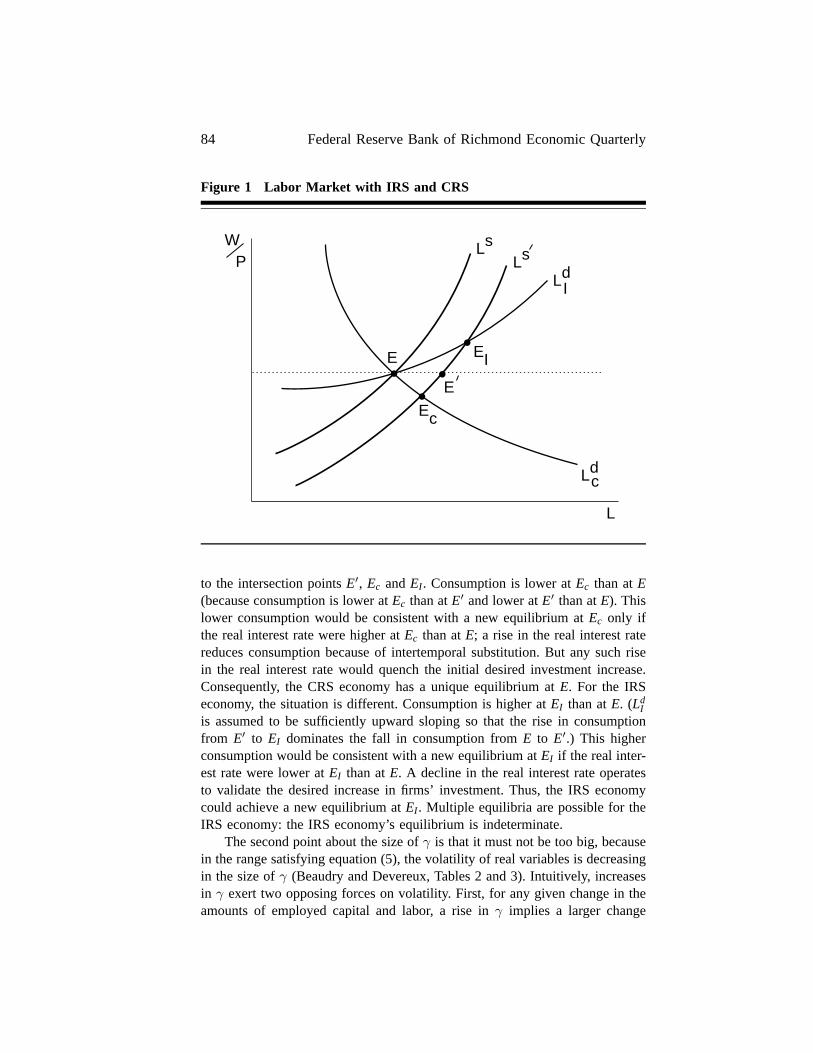
84 Federal Reserve Bank of Richmond Economic Quarterly
Figure 1 Labor Market with IRS and CRS
Ld
Ls
L
E•
•• •
Ec
EI
Ls
E
Ldc
PW
I
+
to the intersection points E′, Ec and EI. Consumption is lower at Ec than at E(because consumption is lower at Ec than at E′ and lower at E′ than at E). Thislower consumption would be consistent with a new equilibrium at Ec only ifthe real interest rate were higher at Ec than at E; a rise in the real interest ratereduces consumption because of intertemporal substitution. But any such risein the real interest rate would quench the initial desired investment increase.Consequently, the CRS economy has a unique equilibrium at E. For the IRSeconomy, the situation is different. Consumption is higher at EI than at E. (Ld
Iis assumed to be sufficiently upward sloping so that the rise in consumptionfrom E′ to EI dominates the fall in consumption from E to E′.) This higherconsumption would be consistent with a new equilibrium at EI if the real inter-est rate were lower at EI than at E. A decline in the real interest rate operatesto validate the desired increase in firms’ investment. Thus, the IRS economycould achieve a new equilibrium at EI. Multiple equilibria are possible for theIRS economy: the IRS economy’s equilibrium is indeterminate.
The second point about the size of γ is that it must not be too big, becausein the range satisfying equation (5), the volatility of real variables is decreasingin the size of γ (Beaudry and Devereux, Tables 2 and 3). Intuitively, increasesin γ exert two opposing forces on volatility. First, for any given change in theamounts of employed capital and labor, a rise in γ implies a larger change
M. G. Finn: Increasing-Returns-to-Scale/Sticky-Price Approach 85
in output and, hence, in most other real variables, such as consumption andinvestment. Second, when γ satisfies equation (5), a higher value of γ causesthe aggregate marginal productivity of labor to rise more quickly with anyincrease in labor. Consequently, smaller changes in labor and hence in capital,output, and most other real variables are needed to equilibrate the economy inresponse to a shock. The second force is the dominant one (again when γ sat-isfies equation [5]), so the volatility of real variables decreases as γ decreases.
The result of the two points concerning the magnitude of γ is that theIRS/sticky-price theory requires γ to lie in a narrow range above γ. This out-come is somewhat troubling for the theory, at least given the current state ofknowledge. Existing empirical evidence is far from precise. Studies by Hall(1990), Caballero and Lyons (1992), Eden and Griliches (1993), Basu andFernald (1994), and Burnside, Eichenbaum, and Rebelo (1995) give point es-timates of γ ranging from one to ten. But perhaps by being explicit about themicrotheoretic foundations of IRS, future research will develop more preciseestimates of γ or will extend the theory in a way that lessens its dependenceon the size of γ.
2. THE STICKY PRICE ASSUMPTION
Once indeterminacy of equilibrium arises because of IRS, the assumption ofsticky prices is made to eliminate that indeterminacy. Alternatively viewed, thesticky price assumption selects one of the multiple equilibria engendered byIRS. This section provides an intuitive explanation of how sticky prices achievedeterminacy of equilibrium and discusses two characteristics of this particularapproach to sticky prices.8
The intermediate goods market is monopolistically competitive. Each inter-mediate goods firm chooses the optimal price of its good each period accordingto the constant markup rule
pt = (1/ρ)MCt , MCt =[Rα
t W(1−α)t ]AΛt
, A > 0, (6)
where p is the nominal price of any intermediate good, MC is the nominalmarginal cost of producing any intermediate good, R is the nominal rentalprice of capital that firms pay, W is the nominal wage of labor faced by firms,A is a parameter, and subscript t denotes time. The marginal cost is increas-ing in an index of factor prices and decreasing in the externality factor thatenhances the productivity of firm inputs. Noting that the absolute value of the
8 The discussion in this section extends easily to Beaudry and Devereux (1993), where IRSare internal to firms, and to Benhabib and Farmer (1992), where the production externality is amonetary one and where firms are perfectly competitive price takers.
86 Federal Reserve Bank of Richmond Economic Quarterly
price elasticity of demand for intermediate goods (by final goods firms) is thesame as the elasticity of substitution of intermediate goods, 1/(1 − ρ), and isthus increasing in ρ, equation (6) shows that the markup is inversely related tothat price elasticity. Equation (6) also shows that all intermediate goods firmschoose the same price because marginal cost is identical across firms.
The final goods market is perfectly competitive. There, because final goodsfirms choose their optimal output each period, the nominal price of the finalgood, denoted by Pt, always equals the nominal marginal cost of its production,which can be shown to equal pt. Therefore
Pt = pt. (7)
The sticky price assumption imposes the requirement that Pt is unresponsive orrigid with respect to any new information that becomes available at time t. Thatis, Pt is assumed to be predetermined at time t. Following equations (6) and (7),pt and MCt must also be predetermined at time t. Thus, with the sticky priceassumption in place, any unanticipated movement in the externality factor attime t, Λt has to be matched by an equal movement in the factor price index,[Rα
t W(1−α)t ] to keep equation (6) intact. This also means that real return to
capital, or the real interest rate, rises at time t if an unanticipated expansionaryforce increases the economy’s output, and thus Λ, at time t. One exampleof such an unanticipated expansionary force is the sudden desire to increaseinvestment that was considered in the experiment of Section 1. Rerunning thatexperiment for the IRS economy under conditions of sticky goods prices showsthat the desired investment increase is vitiated by the increase in the real interestrate. Therefore, the IRS economy with sticky prices has a unique equilibrium.The assumption of sticky prices is responsible for ensuring the determinacy ofequilibrium.
A unique feature of the sticky price assumption is that it is made at the laststage of the modeling procedure. All other assumptions (for instance, those de-scribing preferences, production technologies, and market structure) are made,in standard fashion, at the beginning of the model specification. Next, theequations defining the economy’s equilibrium are deduced. If that equilibriumis indeterminate, the last step of the modeling process is to obtain determinacyof equilibrium by making the sticky price assumption. This unique feature isimportant for at least two reasons.
First, to arrive at the point of assuming sticky prices, the economy’sstructure must give rise to equilibrium indeterminacy. This is somewhat ofa drawback because the required structure is not necessarily easy to justify ontheoretical and empirical grounds. In the IRS/sticky-price theory case, a strongstand needs to be taken on the nature and magnitude of IRS, as discussedearlier.
Second, the approach to sticky prices described above is consistent withall firms optimizing and, consequently, with market clearing. This aspect is
M. G. Finn: Increasing-Returns-to-Scale/Sticky-Price Approach 87
appealing. As mentioned before, all firms choose plans that maximize profitevery period. In particular, intermediate goods firms always choose their pricesaccording to their optimal markup pricing rule (equation [6]). By imposingsticky prices on those optimization rules, optimization continues to hold. Curi-ously, one may imagine, even though it is not literally true, that the intermediategoods firms are choosing prices one period in advance (i.e., choosing pt at timet−1), because firms never want to adjust pt to information that is new at time t.
This approach to sticky prices sharply contrasts with the approach takenin traditional macroeconomic models (e.g., Phelps and Taylor [1977]; Fischer[1977]). The traditional approach does not require initial equilibrium indeter-minacy, and it is inconsistent with full optimization and market clearing. In thatapproach, by assumption, prices truly are set in advance. Consequently, whennew, unanticipated information on demand and supply conditions emerges,those prices are inconsistent with all agents optimizing and thus with marketclearing.
3. SLUGGISH PRICE ADJUSTMENT ANDMONETARY NONNEUTRALITY
The combination of the IRS and sticky price assumptions acts as a powerfulforce to engender sluggish price adjustment and, therefore, monetary nonneu-trality. To explain how this force operates, this section analyzes the effects onthe economy of a permanent increase in the money stock.9
The fundamental role of money is to mitigate the transactions costs arisingfrom the process of allocating factors of production to production activity. Moreexactly, the transactions costs are increasing in the economy’s employment ofcapital and labor and decreasing in real money balances as captured by therelationship
φ(N/P, X) = B(N/P)(1−ν)Xν , B > 0 , v > 1, (8)
where φ is transactions costs (measured in units of output), N is the moneystock, B and ν are parameters, and X is directly related to factor employment
9 The main modification required to apply this explanation to Beaudry and Devereux (1993)is simply to recognize the different transactions role for money in that study. The consequentialdifferent effect of a permanent money stock increase is that nominal interest rates fall in Beaudryand Devereux (1993) while they stay approximately constant in the BD model. The explanation ofmonetary nonneutrality is quite different across the BD and Benhabib and Farmer (1992) models,primarily because the production externality is monetary (and not real) in nature and there isno investment in the latter model. The important point common to both explanations is that theproduction externality ensures that the money supply increase leads to such a sizable expansionof output (at predetermined current prices) and the real demand for money that money marketequilibrium is reestablished by tiny and sluggish increases in future price inflation.

88 Federal Reserve Bank of Richmond Economic Quarterly
according to equation (4). Because of these transactions costs, households re-ceive payments for providing factor services that fall short of the marginalproductivities of those services. In fact, it is straightforward to show that thefactor prices received by households are
W = MC(MPL)[1 − φ2(N/P, X)] and (9)
R = MC(MPK)[1 − φ2(N/P, X)], (10)
where W is the nominal wage of labor received by households; R is the rentalprice of capital received by households; MPL and MPk are the marginal pro-ductivities of L and K in producing the output of the typical intermediate goodsfirm; φ2, the marginal transactions cost of increasing output, denotes the partialderivative of φ with respect to X. Equations (9) and (10), together with theproperties of φ2, make clear that transactions costs shrink the value of factorpayments to households while money holdings help mitigate the extent of thatshrinkage.
If the monetary authority permanently increases the money stock at timet, what will happen at time t? With Pt predetermined at time t, by assumption,the effect of a rise in Nt is a proportionate rise in Nt/Pt. Consequently, themarginal transactions cost of hiring all factors in goods production falls (i.e.,φ2 declines), implying an increase in Wt and Rt (see equations [9] and [10]).This increase in factor payments invokes a rise in households’ desire to supplyfactors to intermediate goods firms. The firms willingly hire the desired increasein factor supply—in a sense they are indifferent because, as explained earlier,both the price and marginal cost of their goods stay constant. The resultantincrease in Kt and Lt expands the output of all goods; thus, Xt rises. On theopposite side of the supply response is the demand response. The increasein Nt/Pt, by raising household wealth, causes an expansion in spending forboth consumption and investment purposes. Denoting aggregate consumptionand investment of the final good by Ct and It, respectively, the rise in Xt
is absorbed by the rise in Ct and It. Because of the presence of IRS, all ofthese expansions in factor employment, output, consumption, and investmentare sizable. Furthermore, IRS together with the large increase in (It implies thatall of these real expansionary effects are strongly propagated into the future.
The sticky price assumption makes current prices predetermined only attime t. Future prices are perfectly free to respond to the money supply increase,starting from time (t + 1). But they do so gradually, and Pt+1 responds hardlyat all. Pt+1 is essentially determined by its role in ensuring equilibrium in themoney market at time t. The money market equilibrium condition is
Nt/Pt = G(Xt, it) , G1 > O , G2 < 0, (11)
where G is a function, Gj is the first derivative of G with respect to its jthargument, (j = 1, 2), and it is the net nominal interest rate. This condition
M. G. Finn: Increasing-Returns-to-Scale/Sticky-Price Approach 89
sets money demand equal to money supply. Stemming from the role of moneyin alleviating the transactions costs arising in production activity, real moneydemand is increasing in Xt. The opportunity cost of money is the forgonenominal interest rate on bonds and so the demand for real money balancesis declining in it. Equation (11) captures both of these effects on real moneyholdings. Furthermore, an intertemporal efficiency condition governing optimalnominal (discount) bond holdings in the economy gives rise to the equilibriumasset-pricing relationship
(1 + it) =
(Pt+1Ct+1
PtCt
)β−1. (12)
The gross nominal interest rate at time t is the product of price inflation andconsumption growth between time t and time (t + 1) and the reciprocal of thesubjective discount factor β.10
While Pt+1 can in principle respond to the increase in Nt, there are two rea-sons why its response is negligible. First, the expansion of Xt is large enoughrelative to that in (Nt/Pt) to create a small incipient excess demand for realbalances. Second, the strong increase in It propagates the increase in Xt sostrongly into the future that consumption grows slightly for a time. The smallincrease in Ct+1/Ct causes a small rise in it that is sufficient to eliminate theincipient excess demand for money. Consequently, Pt+1 does not need to changesignificantly.
IRS and capital accumulation act to strongly propagate, though at a dimin-ishing rate, the real expansionary effect of the money supply increase well intothe future. Similar reasoning explains that prices at time (t + 2) and beyondare also slow to change. It is only after about four periods (at time t + 4),as consumption growth slows and becomes negative, that P eventually andslowly increases. At any time, the increase in future P keeps i approximatelyconstant in face of the small negative consumption growth rates because anapproximately constant i is sufficient to ensure money market equilibrium.Meanwhile, the increase in current P engineers the reductions in N/P that, eachperiod, closely match the declines in X as the economy returns to its steadystate. In the steady state, all real variables take on their original values—theirvalues prior to the increase in Nt—and P rises in the same proportion as Nt.That is, the steady state is neutral with respect to the increase in Nt. Thus,the sluggish price adjustment and consequential monetary nonneutrality areshort-run phenomena.
10 The utility function here is assumed to be an additively separable and logarithmic functionof consumption. Also, for simplicity, the expectations operator is omitted.
90 Federal Reserve Bank of Richmond Economic Quarterly
4. EXPLAINING THE FACTS
How well does the IRS/sticky-price theory explain the empirical evidence?To address this question, this section evaluates the theory along four keydimensions—price, output, nominal interest rate responses to monetary shocks,and the correlation between productivity and employment.
Sluggish Price Adjustment
Empirical evidence indicates that the price level exhibits a slow and lengthyresponse to monetary innovations.11 The theory well captures this evidence.However, it is not entirely clear that the theory’s ability to mimic the dataalong this dimension should be viewed as an explanation. By assumption,prices cannot contemporaneously respond to monetary shocks. Furthermore,the endogenous propagation mechanism delivers sluggish price adjustment insuch a direct fashion that it is almost tantamount to building in sluggish priceadjustment over time by assumption. Admittedly this is somewhat of a finepoint, but it does, at least, prompt less serious evaluation of the theory along thesluggish price dimension and more serious evaluation along other dimensions.
Output Response
Stemming primarily from the assumptions of IRS and sticky prices, the BDmodel has strong implications for the magnitude of the output response toa money shock.12 For example, the model implies that a 1 percentage pointincrease in the money stock contemporaneously causes a 7 percentage pointrise in real output. An output response of this magnitude seems much too big.Sims’s (1980) evidence for the U.S. economy over the postwar period showsthat a 1 percent money stock innovation within the same period causes only a0.42 percent increase in output. Part of the model’s excessive contemporaneousoutput response may be due to the manner in which IRS works. Specifically,by magnifying labor’s exponent in the production function, IRS permits theeconomy to instantly and significantly respond to shocks from any source.
Nominal Interest Rate Response
As described earlier, the BD model predicts essentially no nominal interestrate response to monetary shocks, which seems counterfactual. Strong evi-dence documents the liquidity effect—the negative effect on nominal interestrates exerted by positive monetary innovations (Cochrane 1989). However, the
11 See, for instance, Sims (1980, 1989) for evidence pertaining to the United States.12 This is also true of the Beaudry and Devereux (1993) model. The same strong implications
hold for the Benhabib and Farmer (1992) model, but in that case they stem from the assumptionsof the monetary externality and sticky prices.
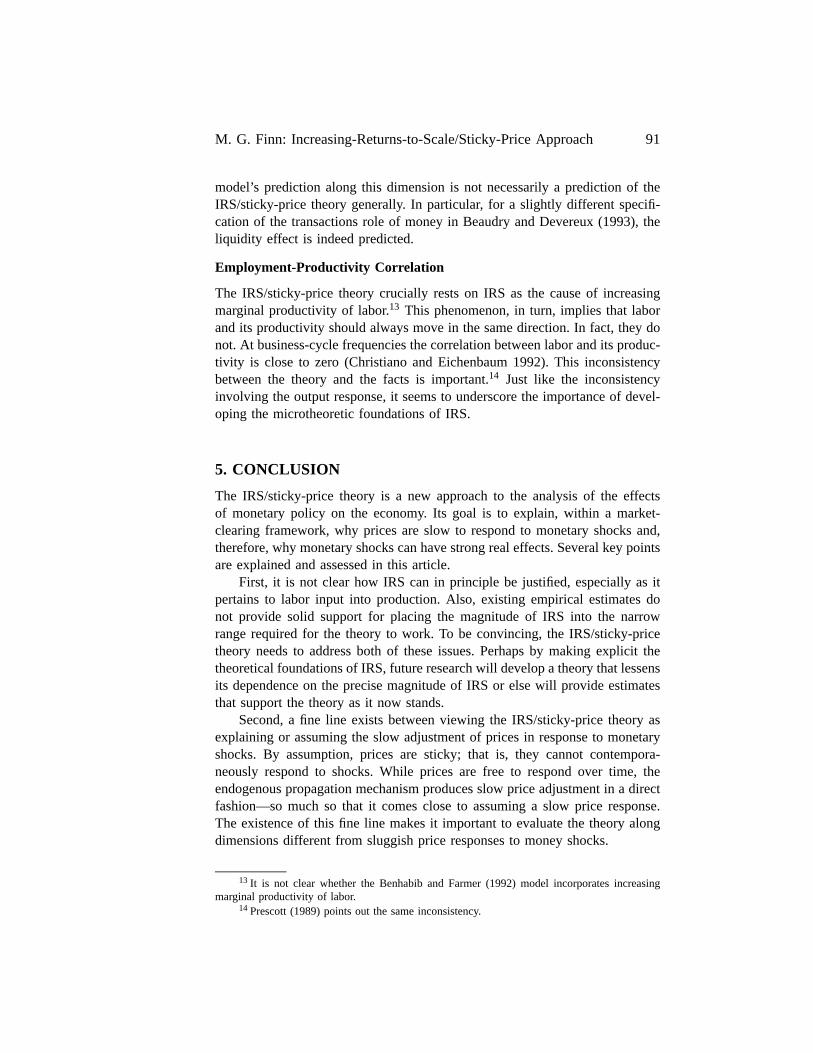
M. G. Finn: Increasing-Returns-to-Scale/Sticky-Price Approach 91
model’s prediction along this dimension is not necessarily a prediction of theIRS/sticky-price theory generally. In particular, for a slightly different specifi-cation of the transactions role of money in Beaudry and Devereux (1993), theliquidity effect is indeed predicted.
Employment-Productivity Correlation
The IRS/sticky-price theory crucially rests on IRS as the cause of increasingmarginal productivity of labor.13 This phenomenon, in turn, implies that laborand its productivity should always move in the same direction. In fact, they donot. At business-cycle frequencies the correlation between labor and its produc-tivity is close to zero (Christiano and Eichenbaum 1992). This inconsistencybetween the theory and the facts is important.14 Just like the inconsistencyinvolving the output response, it seems to underscore the importance of devel-oping the microtheoretic foundations of IRS.
5. CONCLUSION
The IRS/sticky-price theory is a new approach to the analysis of the effectsof monetary policy on the economy. Its goal is to explain, within a market-clearing framework, why prices are slow to respond to monetary shocks and,therefore, why monetary shocks can have strong real effects. Several key pointsare explained and assessed in this article.
First, it is not clear how IRS can in principle be justified, especially as itpertains to labor input into production. Also, existing empirical estimates donot provide solid support for placing the magnitude of IRS into the narrowrange required for the theory to work. To be convincing, the IRS/sticky-pricetheory needs to address both of these issues. Perhaps by making explicit thetheoretical foundations of IRS, future research will develop a theory that lessensits dependence on the precise magnitude of IRS or else will provide estimatesthat support the theory as it now stands.
Second, a fine line exists between viewing the IRS/sticky-price theory asexplaining or assuming the slow adjustment of prices in response to monetaryshocks. By assumption, prices are sticky; that is, they cannot contempora-neously respond to shocks. While prices are free to respond over time, theendogenous propagation mechanism produces slow price adjustment in a directfashion—so much so that it comes close to assuming a slow price response.The existence of this fine line makes it important to evaluate the theory alongdimensions different from sluggish price responses to money shocks.
13 It is not clear whether the Benhabib and Farmer (1992) model incorporates increasingmarginal productivity of labor.
14 Prescott (1989) points out the same inconsistency.

92 Federal Reserve Bank of Richmond Economic Quarterly
Third, in its current state, the IRS/sticky-price theory predicts huge outputresponses to monetary shocks and correlations between labor and its productiv-ity that are noticeably counterfactual. This inconsistency between the theory’spredictions and the facts underscores the importance for the theory to developthe theoretical rationale for IRS.
The IRS/sticky-price theory is innovative and ambitious in tackling thedifficult issue of explaining the effects of money on the economy. The pointsraised in this article suggest, on the one hand, that it would be premature to usethis theory as a basis for understanding the monetary transmission mechanism.In particular, the theory is too inconsistent with key facts to be useful for thatpurpose. On the other hand, the article suggests that it may be fruitful to explorethis theoretical approach further by developing the theory underlying IRS.
REFERENCES
Arrow, Kenneth J. “The Economic Implications of Learning by Doing,” Reviewof Economic Studies, vol. 29 (June 1962), pp. 155–73.
Basu, Susanto, and John G. Fernald. “Constant Returns and Small Markupsin U.S. Manufacturing,” in International Finance Discussion Papers, No.483. Washington: Board of Governors of the Federal Reserve System.
Beaudry, Paul, and Michael B. Devereux. “Money and the Real ExchangeRate with Sticky Prices and Increasing Returns,” Carnegie-RochesterConference Series on Public Policy, vol. 43 (December 1995).
. “Monopolistic Competition, Price Setting, and the Effects ofReal and Monetary Shocks.” Manuscript. University of British Columbia,October 1993.
Benhabib, Jess, and Roger E. A. Farmer. “The Aggregate Effects of MonetaryExternalities.” Manuscript. University of California at Los Angeles, April1992.
Burnside, Craig, Martin Eichenbaum, and Sergio Rebelo. “Capital Utilizationand Returns to Scale.” Manuscript. University of Rochester, February1995.
Caballero, Ricardo J., and Richard K. Lyons. “External Effects in U.S.Procyclical Productivity,” Journal of Monetary Economics, vol. 29 (April1992), pp. 209–25.
Christiano, Lawrence J., and Martin Eichenbaum. “Current Real BusinessCycle Theories and Aggregate Labor Market Fluctuations,” AmericanEconomic Review, vol. 82 (June 1992), pp. 430–50.

M. G. Finn: Increasing-Returns-to-Scale/Sticky-Price Approach 93
Cochrane, John H. “The Return of the Liquidity Effect: A Study of the Short-Run Relation Between Money Growth and Interest Rates,” Journal ofBusiness & Economic Statistics, vol. 7 (January 1989), pp. 75–83.
Eden, Benjamin, and Zvi Griliches. “Productivity, Market Power, and CapacityUtilization When Spot Markets Are Complete,” American EconomicReview, vol. 83 (May 1993), pp. 219–23.
Farmer, Roger E. A. The Macroeconomics of Self-Fulfilling Prophecies.Cambridge, Mass.: MIT Press, 1993.
Finn, Mary G.. “Increasing Returns to Scale and Sticky Prices: Are TheyImportant for Real Exchange Rates? A Comment,” Carnegie-RochesterConference Series on Public Policy, vol. 43 (December 1995).
Fischer, Stanley. “Long-Term Contracts, Rational Expectations, and theOptimal Money Supply Rule,” Journal of Political Economy, vol. 85(February 1977), pp. 191–205.
Hall, Robert E. “Invariance Properties of Solow’s Productivity Residual,”in Peter Diamond, ed., Growth/Productivity/Unemployment: Essays toCelebrate Bob Solow’s Birthday. Cambridge, Mass.: MIT Press, 1990.
Lucas, Robert E. “Supply-Side Economics: An Analytical Review,” OxfordEconomic Papers, vol. 42 (April 1990), pp. 293–316.
Phelps, Edmund S., and John B. Taylor. “Stabilizing Powers of MonetaryPolicy under Rational Expectations,” Journal of Political Economy, vol.85 (February 1977), pp. 163–90.
Prescott, Edward C. “Comment on Building Blocks of Market ClearingBusiness Cycle Models,” Macroeconomics Annual, National Bureau ofEconomic Research, 1989, pp. 287–91.
Rotemberg, Julio J., and Michael Woodford. “Dynamic General EquilibriumModels with Imperfectly Competitive Product Markets,” in ThomasCooley, ed., Frontiers of Business Cycle Research. Princeton, N.J.:Princeton University Press, 1995.
Salyer, Kevin D. “The Macroeconomics of Self-Fulfilling Prophecies: AReview Essay,” Journal of Monetary Economics, vol. 35 (February 1995),pp. 215–42.
Sims, Christopher A. “Models and Their Uses,” American Journal of Agricul-tural Economics, vol. 71 (May 1989), pp. 489–94.
. “Comparison of Interwar and Postwar Business Cycles: Mone-tarism Reconsidered,” American Economic Review, vol. 70 (May 1980),pp. 250–57.