Dependence of Power Performance on Atmospheric Conditions and Possible

Corrections

J.W. WagenaarP.J. Eecen

This paper has been presented at the EWEA 2011,Brussels, Belgium, 14-17 March 2011

ECN-M--11-033 MARCH 2011

Dependence of Power Performance on Atmospheric Conditions and Possible Corrections

J.W. Wagenaarj.wagenaar@ecn.nlECN Wind Energy

P.J. Eeceneecen@ecn.nl

ECN Wind Energy

Abstract

The dependence of the power curve on at-mospheric conditions like air density, tempera-ture, turbulence and vertical wind shear is in-vestigated. For this a 2.5MW ECN research turbine and a nearby meteo mast on ECN’s test field are considered. It is shown that all mentioned atmospheric conditions have effecton either the power curve itself or on the stan-dard deviation of the power.

Correction with respect to air density, as is prescribed by IEC 61400-12-1, and turbulence have been shown to be effective with respect to the standard deviation of the power for (most) interesting wind speeds. Both correc-tions cause the power to be lower than the un-corrected power.

Based on a power law profile, two vertical wind shear corrections are examined and they both, basically, show the same result. For most (in-teresting) wind speeds the standard deviation of the power is decreased, but for some wind speeds an increase of the standard deviation is seen. The power itself is increased, due to the correction.

A so-called rotor averaged wind speed, based on wind speed measurements at multiple heights, is examined to also correct for wind shear. The effect of this correction with respect to the standard deviation of the power is shown to be small for the ECN research tur-bine. Also in this case the power itself is in-creased with respect to the uncorrected power.

Keywords: Power performance, power correc-tions, atmospheric conditions, air density, tur-bulence, vertical wind shear

1. Introduction

The UpWind project (see www.upwind.eu) is a European research project, funded under the EU's Sixth Framework Programme (FP6), that focuses on the necessary up-scaling of wind energy in 2020. Among the problems that hin-der the development of wind energy aremeasurement problems. For example: to ex-perimentally confirm a theoretical improvement in energy production of a few percent of a new design by field experiments is very hard to al-most impossible. As long as convincing field tests have not confirmed the actual improve-ment, industry will not invest to change turbine design. The objective of the Metrology work package (1A2) is to develop metrology tools in wind energy to significantly enhance the qual-ity of measurement and testing techniques.

One of the subjects taken up within the Me-trology work package is the power perform-ance of wind turbines. This work focuses on the analyses of the largest sources of uncer-tainties in power performance testing. It is known that the power performance of a wind turbine depends on atmospheric conditions as for instance the air density. The IEC regula-tions for power performance [1] already in-clude an air density correction. Besides that it is also known that other atmospheric condi-tions play a role as well, such as turbulenceand wind shear, which was already noticed in [2] [3] [4] [5] [6]. Corrections for turbulence and wind shear have been suggested and have been shown to be effective.

We examine the power performance of a 2.5MW turbine on the ECN test field on those atmospheric conditions. This is done in section 2, where the dependence of the power per-formance on the air density (, temperature), stability, turbulence and vertical wind shear is examined. Corrections for these effects are studied in section 3 and the results are con-cluded and discussed in section 4. The work is closely related to the work in the MT12 main-tenance team.

2. Dependence of Power Per-formance on Atmospheric Conditions

Data are taken from the test field of ECN, the ECN Wind Turbine Test station Wieringermeer (EWTW) [7] [8]. It is located in the North East of the Province ‘Noord-Holland’, 1 - 2km West of the lake ‘IJsselmeer’. The test site and its surroundings are characterised by flat terrain.

Among others, the test field consists of 5 re-search turbines named T5 - T9. They have a hub height (H) of 80m, a rotor diameter (D) of 80m and a rated power of 2.5MW. A meteo mast measures wind speed and wind direction at 52m, 80m (hub height) and 108m. From now on, if not mentioned differently, the wind speed and direction always refers to the wind speed and direction at 80m. Also measured are temperature, temperature difference and pressure. Turbines T5 and T6 are suitable to perform power performance measurements [1]. Data from the turbines and the meteo mast have been gathered since 2004. These data involve 10 minute statistics as for instance mean and standard deviation.

For the analysis turbine T6 is used, which is at a distance of 2.5D from the meteo mast. For the entire period of about 6 years of data tak-ing power curves are constructed, either by using scatter data or by using binned values according to IEC regulations [1]. They are given in Figure 2.1. For the scatter data no data selection, other than required for IEC 61400-12-1 [1], has been applied.

Figure 2.1 Power curve for turbine T6.

We note the three ‘tails’ in Figure 2.1 for wind speeds above 15m/s. In the remainder differ-ent (sub) data sets will be considered and the distribution of the data points for wind speeds above 15m/s over the three ‘tails’ may be dif-ferent from one situation to another. This influ-ences the standard deviation of the power. Therefore, when comparing standard devia-tions of the power, wind speeds above 15m/s are not considered in this paper.

Because of the huge database it is possible to select data based on certain atmospheric con-ditions to see whether the power curve de-pends on these conditions. The atmospheric conditions considered are air density, tempera-ture, atmospheric stability, turbulence and ver-tical wind shear.

2.1 Air densityThe power that a turbine can extract from a volume of wind is [9]

3

21 UAcP p , (1)

where U is the horizontal wind speed, A is the rotor swept area, ρ is the air density and cp is the power coefficient. P is the power. Clearly, the power depends on the air density and therefore also the power curve does. The air density values encountered at the site1 are mostly between 1.20 kg/m3 and 1.27 kg/m3

and the mean value is 1.237 kg/m3.

Power curves for various values of the air den-sity can clearly be distinguished. The maxi-mum difference with the power curve for all densities occurs for the power curve for

1 The air densities encountered are extracted from the same data set as used for the power performance. This will also be the case for the other atmospheric quantities.

ρ=1.205 kg/m3. This difference is at most 4% for (unnormalized) wind speeds above 5m/s.

Also for different values of temperature power curves can be distinguished. However, be-cause the air density is calculated from tem-perature (and pressure) measurements, it is obvious that the two are related. This is alsoreflected in the power curves.

2.2 StabilityThe stability of the atmosphere is determined by means of the environmental lapse rate:

-dT/dh < 6K/km = stable atmospheric conditions

6K/km < -dT/dh < 10K/km = condi-tionally unstable atmospheric condi-tions

-dT/dh > 10K/km = unstable atmospheric conditions,

where T is the temperature and h is the height. The lapse rate is determined using the tem-perature difference instrument, which meas-ures the temperature difference between a height of 37m and 10m. It is observed that un-stable conditions happen the most during day-time and during summer. For stable conditions the opposite is valid. The frequency of occur-rence of stable conditions is about 7 times higher than that for conditionally stable or un-stable conditions.

Power curves for stable, unstable and all at-mospheric conditions have been constructed and, generally, the differences between the various power curves are small. For wind speeds above, say, 6m/s the difference be-tween the power for all atmospheric conditions and stable conditions and the between the power curve all atmospheric conditions and unstable conditions is lower than about 2%.

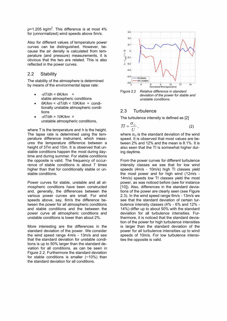
More interesting are the differences in the standard deviation of the power. We consider the wind speed range 4m/s - 13m/s and see that the standard deviation for unstable condi-tions is up to 50% larger than the standard de-viation for all conditions, as can be seen in Figure 2.2. Furthermore the standard deviation for stable conditions is smaller (~10%) than the standard deviation for all conditions.

Figure 2.2 Relative difference in standard deviation of the power for stable and unstable conditions.

2.3 TurbulenceThe turbulence intensity is defined as [2]

UTI U , (2)

where σU is the standard deviation of the wind speed. It is observed that most values are be-tween 2% and 12% and the mean is 8.1%. It is also seen that the TI is somewhat higher dur-ing daytime.

From the power curves for different turbulence intensity classes we see that for low wind speeds (4m/s - 10m/s) high TI classes yield the most power and for high wind (12m/s -14m/s) speeds low TI classes yield the most power, as was noticed before (see for instance [10]). Also, differences in the standard devia-tions of the power are clearly seen (see Figure 2.3). In the wind speed range 6m/s - 13m/s we see that the standard deviation of certain tur-bulence intensity classes (4% - 6% and 12% -14%) differ up to about 50% with the standard deviation for all turbulence intensities. Fur-thermore, it is noticed that the standard devia-tion of the power for high turbulence intensities is larger than the standard deviation of the power for all turbulence intensities up to wind speeds of 10m/s. For low turbulence intensi-ties the opposite is valid.

Figure 2.3 Relative difference in standard deviation of the power for different TI classes.

2.4 Vertical wind shearVertical wind shear is important because wind turbines become larger and larger. It is there-fore questionable whether the hub height windspeed is still representative.

The vertical wind shear can be quantified by assuming a power law profile [9]

rr z

zzUzU )()( , (3)

where U(z) is the horizontal wind speed at height z. The subscript r indicates the refer-ence height and α is a dimensionless constant.

Because the horizontal wind speed is meas-ured at three different heights, two α expo-nents are determined: α1 for the heights 108m and 80m and α2 for the heights 80m and 52m. Both αi exponents are distributed over bins of 0.1 wide. Those cases are considered where both αi exponents are in the same bin. In 1/3 of all possibilities the wind shear shows a profile as assumed in (3). It is noticed that most val-ues are within α=0.1 and α=0.4. The mean value is α=0.3.

The differences between the power curves for various values of α with respect to the power curve for all α are relatively small; they are a few percent. However, differences in the stan-dard deviation of the power are clearly seen, as can be seen from Figure 2.4. In the wind speed range, say, 5m/s - 13m/s the standard deviation of the power for different values of α differs up to about 30% with the standard de-viation of the power for all values of α. It is also seen in this same wind speed range that the standard deviation for a low values of α (α=0.1) is larger than the standard deviation

for all values of α and the standard deviation for a higher value of α (α=0.3, 0.5) is smaller.

Figure 2.4 Relative difference in standard deviation of the power for different values of α.

2.5 Cross correlationsAlthough stability, turbulence and vertical wind shear are treated separately in the foregoing, it may be expected that these phenomena are correlated.

It is noticed that low values of α (say α=0.1) occur most frequent for unstable conditions and high turbulence intensity and high values of α (say α=0.3, 0.4) occur most frequent for stable conditions and low turbulence intensity. Also, in the former case the distribution of α is much sharper.

These phenomena are explained by the fact that for unstable conditions and high turbu-lence different layers of air mix, which in-creases the correlation of the horizontal wind speeds at different heights. This decreases the value of α and broadens the distribution. For a value of α=0 all horizontal wind speeds at dif-ferent heights are the same.

3. Corrections for Impact of Atmospheric Conditions on Power Performance

Since it is shown in section 2 that the power curve depends on atmospheric conditions it is desirable to correct for these conditions such that the power curve becomes independent ofthese conditions or that the dependence of the power curve on these conditions reduces. As mentioned, [1] already prescribes an air den-sity correction. Besides that we also consider turbulence and vertical wind shear correction.

A correction with respect to stability is not con-sidered, however, as we have seen, stability is correlated to turbulence and wind shear.

3.1 Air densityThe ECN research turbines are pitch-regulated. Therefore, according to [1], the air density normalization is applied to the wind speed

3/1

0

UU norm . (4)

Here, Unorm is the normalized wind speed and ρ0 is the reference air density. As a reference the sea level air density is taken (1.225 kg/m3).

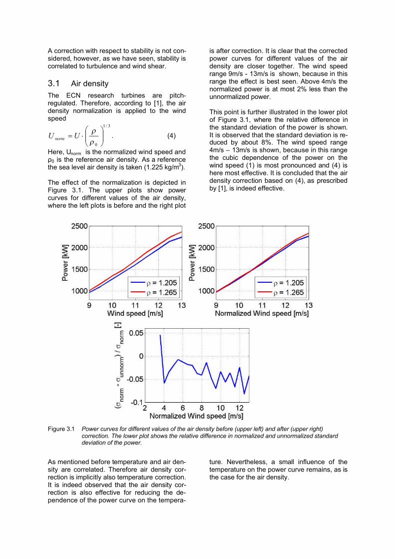
The effect of the normalization is depicted in Figure 3.1. The upper plots show power curves for different values of the air density, where the left plots is before and the right plot

is after correction. It is clear that the corrected power curves for different values of the air density are closer together. The wind speed range 9m/s - 13m/s is shown, because in thisrange the effect is best seen. Above 4m/s the normalized power is at most 2% less than the unnormalized power.

This point is further illustrated in the lower plot of Figure 3.1, where the relative difference in the standard deviation of the power is shown. It is observed that the standard deviation is re-duced by about 8%. The wind speed range 4m/s – 13m/s is shown, because in this range the cubic dependence of the power on the wind speed (1) is most pronounced and (4) is here most effective. It is concluded that the air density correction based on (4), as prescribed by [1], is indeed effective.

Figure 3.1 Power curves for different values of the air density before (upper left) and after (upper right) correction. The lower plot shows the relative difference in normalized and unnormalized standard deviation of the power.

As mentioned before temperature and air den-sity are correlated. Therefore air density cor-rection is implicitly also temperature correction.It is indeed observed that the air density cor-rection is also effective for reducing the de-pendence of the power curve on the tempera-

ture. Nevertheless, a small influence of the temperature on the power curve remains, as is the case for the air density.

3.2 TurbulenceIn (1) it is shown that the power depends cubi-cally on the wind speed. Implicitly, the third power of the averaged wind speed was con-sidered. However, the average of the power depends on the average of the cubed wind speed. It can be shown [5] that in this way a correction factor is added or, equivalently, a corrected wind speed is defined

3/12

31

UUU U

normcorr

. (5)

Here, σU/U is the TI (2).

The turbulence corrected power is shown in Figure 3.2 for low and high values of TI. Also shown is the uncorrected power for the samevalues of TI for comparison. The two curves are in the corrected case somewhat closer to-gether with respect to the uncorrected case. This is made more quantitative in the relative

difference in the standard deviation of the power before and after the correction, also shown in Figure 3.2. Here, the standard devia-tion of the corrected power is for almost all wind speeds in the range up to 12m/s lower than the standard deviation of the uncorrected power. A reduction up to 9% is seen. The cor-rection (5) is based on the cubical dependence of the power on the wind speed. This behav-iour is most pronounced in the mentioned wind speed range. Therefore, it is concluded that the turbulence correction (5) is effective.

A difference in corrected and uncorrected power is observed up to 7%; for higher wind speeds (>6m/s) this is less than 2%. For al-most all wind speeds the corrected power is lower than the uncorrected power. This is caused by the fact that the corrected wind speed is always larger that the uncorrected wind speed, due to the correction as given by (5).

Figure 3.2 Power curves for different TI classes before (upper left) and after (upper right) correction. The lower plot shows the relative difference in uncorrected and corrected standard deviation of the power.

3.3 Vertical wind shearTo correct for the wind shear various ap-proaches are considered. The first approach is to determine the power law profile (3), i.e. to determine α, based on the measurements and to correct the wind speeds according to this

profile. An other approach is to directly use the measurements at multiple heights in a redefini-tion of the wind speed.

Wind shear corrected wind speed:Attempts to correct for vertical wind shear are sought in the assumption of a power law pro-

file of the wind shear. Here, we first average the (horizontal) wind speed vertically

11

2/

2/,

21

23

11)(

)(21

HU

dzzUR

UDH

DHvertave

, (6)

where U(z) is defined in (1) and (3) and zr = H. Furthermore, it has been used that H=D. From (6) it is obvious that the hub height wind speed U(H) is α corrected based on the profile it is experiencing. These corrections are in the range 0.989 - 1.0353 for the α values in the range -0.5 to 1.

A second possibility is to average the wind speed over the rotor plane [4]. Again, a power law wind profile is assumed (3)

dyyyHU

dAzUA

UDH

DHrotave

12112)(

)(1

1

1

2

2/

2/,

,(7)

where y is a dummy integration variable. Also in this case the hub height wind speed is αcorrected based on the profile it is experienc-ing. Now, the corrections are in the range 0.9918 - 1.0259 for the same α range as be-fore.

It is observed that both corrections have more are less the same effect.

A difference between the corrected and uncor-rected power up to 12 % is seen. For wind speeds, say, above 5m/s the corrected power differs less than 3% from the uncorrected power. In all cases the corrected power is lar-ger than the uncorrected power.

In Figure 3.3 the relative difference in the standard deviation of the corrected and uncor-rected power is shown. For most wind speeds a decrease of the standard deviation of at most 10% is seen as a result of the α correc-tion. However, for some wind speeds in theregime up to 12m/s an increase is seen.

Figure 3.3 Relative difference in uncorrected and corrected standard deviation of the power.

Rotor averaged wind speed:Besides assuming a power law profile of the vertical wind shear also real measurements at multiple heights can be used by redefining the wind speed. At the meteo mast the wind speed is measured at three different heights: 52m, 80m and 108m. With these measurements a so-called rotor averaged wind speed is de-fined, similar to for instance [5] [11]

108108808052521 UAUAUAA

Uaveragedrotor

, (8)

Here, Urotor-averaged is the rotor averaged wind speed and U52 , U80 and U108 are the wind speed at the various height. A is the entire ro-tor swept area and A52, A80 and A108 are differ-ent sections of this area defined by height x(see Figure 3.4).

2RA

42arcsin2

222

80xRx

RxRA

,(9)

280

10852AAAA

We notice that for x=80m the rotor averaged wind speed is equal to the wind speed at hub height.

Figure 3.4 Rotor swept area divided in three sections.

The different corrected power curves differ up to 4% for wind speeds above 6m/s from the uncorrected power curve. In practically all cases (all x-values and wind speeds) the cor-rected power is larger than the uncorrected power.

Based on Figure 3.5, only for x=60m the stan-dard deviation of the power shows for most wind speeds a decrease of about 3%. In prac-tice, for values of x above 50m the standard deviation of the power is decreased about a few percent. Therefore, this correction is only effective for these values of x, although the ef-fect is relatively small.

Figure 3.5 Relative difference in standard deviation of the power for the different values of x.

4. Conclusion and Discussion

All atmospheric conditions that have been considered, i.e. air density, temperature, turbu-

lence and vertical wind shear, have been shown to have effect on either the power curves themselves or on the standard devia-tion of the power.

Corrections with respect to air density, as pre-scribed by [1], turbulence and vertical wind shear are examined. Corrections with respect to temperature and stability are not consid-ered. This because temperature is correlated to air density and stability is correlated to tur-bulence and wind shear, as we have seen.

Correction with respect to air density (4) and turbulence (5) have been shown to be effectivefor (most) wind speeds in the range where the cubic dependence of the power on the wind speed is most pronounced, say 4m/s - 12m/s. In case of the air density the standard devia-tion is reduced up to about 8% and in case of the turbulence a reduction up to about 9% is seen. Both corrections cause the power to be lower than the uncorrected power. Above 6m/s these differences are at most 2%.

Both vertical wind shear corrections based on the α parameter basically show the same re-sult. In the most interesting wind speed regime the standard deviations are in most cases re-duced up to about 10%, but for some wind speeds a increase of the standard deviation is seen.

In case of the rotor averaged wind speed cor-rection, only for x values above 50m an im-provement in the standard deviation is seen ofabout 3%. The effect of the correction is con-sidered to be small.

All considered wind shear corrections, based on a power law profile and based on meas-urements at multiple heights, cause the power to be higher than the uncorrected power. These differences are less than 4% above wind speeds of 6m/s.

Acknowledgements

This work was performed in the framework of the project UpWind FP6; work package 1A2 Metrology.

References

[1] “IEC 61400-12-1:2005(e): Wind tur-bines - Part 12-1: Power performance measurements of electricity producing wind turbines,” 2005.

[2] Elliott and Cadogan, “Effects of wind shear and turbulence on wind turbine power curves,” Proceedings European Community Wind Energy Conference, 1990.

[3] Pedersen, Gjerding, Ingham, Enevold-sen, Hansen, and Jorgensen, “Wind turbine power performance verification in complex terrain and wind farms,” Riso Report, April 2002. Riso-R-1330(EN).

[4] Sumner and Masson, “Influence of at-mospheric stability on wind turbine power performance curves,” Journal of Solar Energy Engineering, vol. 128, 2006.

[5] Antoniou, Wagner, Pedersen, Paulsen, Madsen, Jorgensen, Thomsen, Enevoldsen, and Thesbjerg, “Influence of wind characteristics on turbine per-formance,” Poceedings EWEC, 2007.

[6] Rareshide, Tindal, Johnson, Graves, Simpson, Bleeg, Harris, and Schoborg, “Effects of complex wind regimes on turbine performance”, Proceedings AWEA Windpower, 2009.

[7] P.J. Eecen, et al., “Measurements at the ECN Wind Turbine Test Location Wieringermeer”, Proceedings EWEC,2006, ECN-RX--06-055.

[8] P. J. Eecen and J. P. Verhoef, “EWTW Meteorological database. Description June 2003 - May 2007,” ECN Report, June 2007. ECN-E–07-041.

[9] Manwell, McGowan, and Rogers, Wind Energy Explained, Theory, Design and Application. Wiley, 2002.

[10] Kaiser, Hohlen and Langreder, “Turbu-lence Correction for Power Curve”, Proceedings EWEC, 2003.

[11] Wagner, et al., “The Influence of Wind Speed Profile on Wind Turbine Per-formance Measurements”, Wind En-ergy, vol. 12, 2009.

12 ECN-0--10-000

1. IEC 61400-12-1:2005(E); Wind turbines – Part 12-1:Power performance measurements of electricity producingwind turbines

2. Antoniou, et al . “Influence of wind characteristics on turbine performance,” Proceedings EWEC, 2007.3. Sumner and Masson, “Influence of atmospheric stability on wind turbine power performance curves,” Journal of

Solar Energy Engineering, vol. 128, 2006.4. Wagner, et al., “The Influence of W ind Speed Profile on Wind Turbine Performance Measurements”, Wind

Energy, vol. 12, 2009.

Data are taken from the research wind turbines at ECN Wind Turbine Test station Wieringermeer (EWTW) [3] since 2004. The test site is located 1 – 2km West of the lake ‘IJsselmeer’ and the terrain and its surroundings are characterised as flat.

Introduction

Power Performance and Atmospheric Conditions

J.W. Wagenaar and P.J. EecenEnergy Research Centre of the Netherlands

P.O. Box 1, 1755 ZG Petten, The Netherlands. E-mail: j.wagenaar@ecn.nl

PO. 463

Results

Data and Atmospheric Conditions

Corrections

References

EWEA 2011, Brussels, Belgium: Europe’s Premier Wind Energy Event

The demonstration of the value of innovations in wind energy applications is difficultdue to the relatively large uncertainty in measurements – the main reason is the natureof the source of energy: the turbulent wind

This work focuses on the analyses of sources of uncertainties in power performancetesting. Based on an extensive set of measured data at ECN test site, the dependenceof the power curve on atmospheric conditions is determined:

• Air density• Turbulence• Vertical wind shear

Possible correction methods are investigated to reduce the uncertainty in powerperformance measurements. The work is closely related to the work in the MT12maintenance team and MEASNET.

3/1

0

UUnorm

3/12

31

UUU U

normcorr

dAzUA

U

dzzUR

U

HzHUzU

DH

DHrotave

DH

DHvertave

)(1

)(21

)()(

2/

2/,

2/

2/,

Air density correction (IEC):IEC regulations [1] prescribe to correct the wind speed for air density for pitchregulated turbines.

Turbulence correction:Considering the average of the cubed wind speed, it can be shown [2] that a TI-corrected wind speed is defined, where the turbulence intensity TI=s U/U.

Vertical wind shear correction: (II) Measurements at multiple heightsWind speed measurements at multiple heights are directly used in a redefinition [2][4]of the wind speed.

2

42arcsin2

:)(

:)(

8010852

222

80

2

3/13108108

38080

35252

,

10810880805252

AAAA

xRxRxRA

RA

AUA

AUA

AUA

Ub

AUA

AUA

AUAUa

cubeaveragedrotor

averagedrotor

Vertical wind shear correction: (I) Power law profileThe horizontal wind speed is corrected either by vertical averaging or by averaging over therotor plane [3], based on a power law profile it is experiencing.

Air density (IEC):

• Most effective in wind speed range 4m/s – 12m/s

• Power is decreased by at most 2% for wind speeds above 6m/s

• Standard deviation is reduced up to 8%

Turbulence:

• Most effective in wind speed range 4m/s – 12m/s

• Power is decreased by at most 2% for wind speeds above 6m/s

• Standard deviation is reduced up to 9%

Vertical wind shear: (I) Power law

• Both power law corrections have the same effect

• Power is increased by at most 4% for wind speeds above 6m/s

• Standard deviation is reduced up to 10% for most wind speeds

• For some wind speeds an increase in standard deviation is seen

Vertical wind shear: (IIa) Measurements at multiple heights

• Only effective for x>50m• Power is increased by at most 4% for wind

speeds above 6m/s• Standard deviation is reduced up to 3%

Turbine:

• 2.5MW rated power• Hub height (H) 80m• Rotor diameter (D=2R)

80m

Meteo mast:

• Wind speed 52m, 80m and 108m• Wind direction 52m, 80m and 108m • Temperature and temperature difference• Pressure

Conclusions

• The air density and turbulence corrections are most effective. s P is reduced up to 9% - 10% for wind speeds of 4m/s - 12m/s.

• Wind shear correction:• The power law correction reduces s P up to 10%, but shows

for some wind speeds an increase.• The multiple measurements (IIa) correction reduces sP up to

3% for x>50m.• The multiple measurements (IIb) correction reduces sP up to

5% for x>40m.

• Changes in power are at most +/- 4% for wind speeds above 6m/s.

Vertical wind shear: (IIb) Measurements at multiple heights (ongoing research)

• Power is increased by at most 1% for wind speeds above 6m/s (x>40m)

• Standard deviation is reduced up to 5%• Better than the linear case (IIa)