Formulation and numerical implementation of micro-scaleboundary conditions for particle aggregates

J. Liu, E. Bosco, A.S.J. Suiker∗.

Department of the Built Environment,Eindhoven University of Technology, The Netherlands

February 13, 2017

Abstract

Novel numerical algorithms are presented for the implementation of micro-scale boundary conditions ofparticle aggregates modelled with the discrete element method. The algorithms are based on a servo-controlmethodology, using a feedback principle comparable to that of algorithms commonly applied within controltheory of dynamic systems. The boundary conditions are defined in accordance with the large deformationtheory, and are imposed on a frame of boundary particles surrounding the interior granular micro-structure.Following the formulation presented in Miehe et al., (2010), Int. J. Num. Meth. Engng. 83, pp. 1206-1236, first three types of classical boundary conditions are considered, in accordance with i) a homogeneousdeformation and zero particle rotation (D), ii) a periodic particle displacement and rotation (P), and iii) auniform particle force and free particle rotation (T). The algorithms can be straightforwardly combined withcommercially available discrete element codes, thereby enabling the determination of the solution of boundary-value problems at the micro-scale only, or at multiple scales via a micro-to-macro coupling with a finite elementmodel. The performance of the algorithms is tested by means of discrete element method simulations onregular monodisperse packings and irregular polydisperse packings composed of frictional particles, whichwere subjected to various loading paths. The simulations provide responses with the typical stiff and softbounds for the (D) and (T) boundary conditions, respectively, and illustrate for the (P) boundary condition arelatively fast convergence of the apparent macroscopic properties under an increasing packing size. Finally, ahomogenization framework is derived for the implementation of mixed (D)-(P)-(T) boundary conditions thatsatisfy the Hill-Mandel micro-heterogeneity condition on energy consistency at the micro- and macro-scalesof the granular system. The numerical algorithm for the mixed boundary conditions is developed and testedfor the case of an infinite layer subjected to a vertical compressive stress and a horizontal shear deformation,whereby the response computed for a layer of cohesive particles is compared against that for a layer of frictionalparticles.

keywords: granular materials, multi-scale modeling, discrete element method, servo-control algorithm,boundary conditions

1 Introduction

The accurate computation of the non-linear failure and deformation behavior of heterogeneous granular systemscommonly requires a resolution of the complex mechanical interactions and deformation mechanisms at theparticle scale, which can be adequately accounted for by using the discrete element method (DEM), see e.g.,[1, 2, 3, 4, 5, 6, 7, 8, 9, 10] and references therein. For practical granular systems composed of a vast numberof particles, however, it is infeasible to simulate each particle as an individual discrete object, since this leadsto DEM models with an enormously large number of degrees of freedom, and consequently, to impracticalcomputation times. To circumvent this problem, advanced multi-scale frameworks have been developed, wherethe mechanical responses at the particle micro-scale and the structural macro-scale are hierarchically coupledin an computationally economical fashion. This is accomplished by simulating the macro-scale problem underconsideration with the finite element method (FEM), whereby in every integration point the response to thecorresponding deformation is calculated by means of a DEM model that accurately and efficiently represents thecomplex particle behavior at the micro-scale. Examples of coupled FEM-DEM approaches for granular materialscan be found in [11, 12, 13, 14, 15], illustrating the use of various averaging theorems for relating force

∗Correspondence to: a.s.j.suiker@tue.nl, Department of the Built Environment, Eindhoven University of Technology, P.O. Box 513, 5600MB Eindhoven, The Netherlands.

1

arX

iv:1

612.

0700

6v2

[co

nd-m

at.s

oft]

24

Feb

2017

and displacement measures at the particle micro-scale to stress and strain measures at the structural macro-scale. Specific aspects that should deserve more attention in FEM-DEM homogenization methods, but often areneglected for reasons of simplicity, refer to i) the Hill-Mandel micro-heterogeneity condition, which enforcesconsistency of energy at the micro- and macro-scales, ii) the effect of particle rotations in the formulation ofmicro-to-macro scale-transitions, and iii) a rigorous generalization of the multi-scale approach within the theoryof large deformations.

The computational homogenization framework presented in [16] does include the three aspects mentionedabove, and calculates the micro-scale response of a granular packing with a DEM model equipped with a frameof boundary particles at which the finite deformation following from the macro-scale is imposed. The formu-lation considers three types of micro-scale boundary conditions for the boundary particles, namely i) homoge-neous deformation and zero particle rotation (D), ii) periodic particle displacements and rotations (P), and iii)uniform particle force and free particle rotation (T), where the abbreviations (D), (P) and (T) are adopted fromanalogous, classical boundary conditions used in continuum homogenization theories, referring to the displace-ment, periodic and traction boundary conditions, respectively. The numerical implementation of the boundaryconditions in [16] is done via a penalty method, where the violation of the boundary conditions is punishedby increasing the total virtual work of the particle packing, through the introduction of additional forces andmoments on the frame of boundary particles. Although the algorithm presented in [16] has been nicely gen-eralized for the three types of boundary conditions in a mathematically elegant and transparent fashion, dueto the nature of the penalty method the expression for the homogenized stress of the particle packing becomesexplicitly dependent on the value of the penalty parameter, and thereby looses its physical interpretation. Inaddition, in DEM models the penalty parameter may be difficult to control and must be chosen sufficiently largein order for the penalty function to be effective, which may induce numerical instabilities [17, 18]. Anothercharacteristic of the penalty method is that it requires the constraint equations to be satisfied “approximately”instead of “exactly”, whereby the accuracy of the approximation is determined by the magnitude of the penaltyparameter. As a consequence, the limit case at which the boundary conditions are met exactly is not rigor-ously retrieved from the formulation, since the homogenized stress of the particle packing then vanishes, seeexpression (44) in [16].

In order to improve on the algorithmic drawbacks mentioned above, in the present communication an alter-native numerical algorithm is proposed for the implementation of the homogenization framework presented in[16]. This algorithm is based on a servo-control methodology, using a feedback principle comparable to that ofalgorithms commonly applied within control theory of dynamic systems [19]. Accordingly, the displacementsand rotations of the particles of the boundary frame are iteratively adapted from a gradually diminishing dis-crepancy between the measured and desired values of the micro-scale boundary condition. A strong point ofthis approach is that it is relatively simple to implement, and only affects the interface communicating informa-tion between the macro-scale FEM and micro-scale DEM models. In other words, it does not require internalmodifications of the FEM and DEM source codes, so that the approach can also be combined with commerciallyavailable software for which the user typically has no access to the source code. In addition to its simplicity, theservo-control algorithm preserves the physical interpretation of the homogenized stress measure derived for theparticle packing, and furnishes a realistic value for the stress in the limit case at which the micro-scale boundarycondition is met exactly. It is noted that the algorithm only considers the (P) and (T) boundary conditions, sincefor a macro-scale problem discretized with a displacement-based FEM code, the (D) boundary condition can beimplemented in a straightforward fashion, without the use of iterations.

Apart from providing servo-control algorithms for the individual (P) and (T) boundary conditions, a novelformulation for mixed (D)-(P)-(T) boundary conditions is derived, and subsequently cast into a numerical for-malism. The formulation is proven to satisfy the Hill-Mandel micro-heterogeneity condition, and therefore isvery useful for i) a consistent derivation of macro-scale constitutive relations from standard material tests onparticle aggregates subjected to any combination of (D)-, (P)- and/or (T)-type boundary conditions, and ii) theefficient computation of the homogenized response of large-scale particle aggregates characterized by a spatialperiodicity in one or two directions, i.e., granular layers exposed to uniform (D) and/or (T) boundary conditionsat their top and bottom surfaces. It will be demonstrated that the formulation allows to impose the (D) and (T)boundary conditions both at separate and identical parts of the layer boundary, where in the latter case the (D)and (T) contributions obviously need to be applied along different orthonormal directions.

The performance of the servo-control algorithms developed for the various micro-scale boundary conditionsis tested by using monodisperse and polydisperse frictional and cohesive packings composed of two-dimensio-nal, circular particles and subjected to various loading paths. These examples illustrate the basic features ofeach of the boundary conditions in full detail. Despite the focus on two-dimensional particle systems, it shouldbe mentioned that the extension of the present framework towards three-dimensional granular systems is trivial,and can be made without the introduction of additional prerequisites.

The paper is organized as follows. Section 2 presents a review of the numerical homogenization frameworkfor particle aggregates, and outlines the formulations of the micro-scale (D), (P) and (T) boundary conditionsproposed in [16]. Section 3 discusses the numerical implementation of the micro-scale boundary conditions,

2

where for the (P) and (T) boundary conditions two different servo-control algorithms are presented, whichinclude or not an initial prediction of the displacements of the boundary particles based on their positionscalculated at the previous loading step. In Section 4 the performance of the numerical algorithms is testedon monodisperse and polydisperse frictional packings subjected to various loading paths. The numerical re-sults clearly illustrate the characteristic differences in response for the three types of boundary conditions, andshow their response convergence behavior under increasing sample size. Section 5 presents the formulationfor the mixed boundary conditions, and provides the details of the servo-control algorithm and its numericalperformance for the cases of infinite frictional and cohesive granular layers loaded by a vertical compressivestress, and subsequently subjected to a horizontal shear deformation. Some concluding remarks are providedin Section 6.

In terms of notation, the cross product and dyadic product of two vectors are, respectively, designated asa×b = eijkaibjek and a⊗b = aibjei⊗ ej , where eijk is the permutation symbol, ei, ej and ek are unit vectorsin a Cartesian vector basis, and Einstein’s summation convention is used on repeated tensor indices. The innerproduct between two vectors is given by a ·b = aibi, and between two second-order tensors by A : B = AijBij .The action of a second-order tensor on a vector is indicated as A · b = Aijbjei. The superscript T is used toindicate the transpose of a vector or a tensor. Further, I = δijei ⊗ ej denotes the second-order identity tensor,with δij the Kronecker delta symbol.

Since the present study focuses on two-dimensional particle aggregates, throughout the paper the dimen-sions related to volume, area, stress and mass density are consistently presented in their reduced form aslength2, length, force/length and mass/length2, respectively.

2 Micro-macro transitions for particle aggregates

2.1 Micro-scale geometry

The initial micro-scale granular system is characterized by a two-dimensional square domain of P + Q rigidparticles, which are partitioned into P inner particles Pp, with p = 1, .., P , and Q boundary particles Pq, withq = 1, .., Q, colored in yellow and red in Figure 1(a), respectively. The boundary particles can be further splitinto corner particles Pc with c = 1, .., 4 and the remaining edge particles Pe with e = 1, .., E = Q − 4. Theinitial interior domain V comprises the inner particles with their center points as Xp ∈ Pp with p = 1, .., P . Theboundary ∂V is defined by the boundary particles, whose center points in the initial configuration are Xq ∈ Pqwith q = 1, .., Q. The macroscopic deformation of the granular microstructure is imposed via the frame ofboundary particles Pq, as a result of which the center points of the inner and boundary particles become locatedat xp and xq, respectively, see Figure 1(b). In the current configuration, the boundary particles Pq are subjectedto boundary forces aq, boundary moments mq, and particle contact forces f cq , see Figure 1(c), while the innerparticles Pp are subjected to particle contact forces f cp , see Figure 1(d), with the superscript c denoting a contactwith a neighbour particle.

The macroscopic response of a granular assembly is derived by transforming relevant principles used in first-order homogenization theories [20, 21, 22, 23] from a continuous setting to a discrete setting. Accordingly, atthe centroids of the boundary particles Pq the finite area vectors Aq and forces aq are derived from infinitesimalarea vectors and forces, respectively,

∫

∂V

Nds→ Aq and∫

∂V

t ds→ aq for q = 1..., Q , (1)

with N the vector pointing in the outward normal direction of the boundary ∂V of the initial particle volumeV , t being the boundary traction, and ds indicating an infinitesimal part of the boundary surface. Variousexpressions for Aq have been presented in the literature, see e.g., [24, 25]. In the present communication theinitial area vector is computed by accounting for the different radii of the boundary particles:

Aq =Rq

Rq +Rq−1(Xq −Xq−1)× e3 +

RqRq +Rq+1

(Xq+1 −Xq)× e3 , (2)

where Rq+1, Rq and Rq−1 are the radii of adjacent boundary particles q + 1, q and q − 1, respectively. Further,e3 represents the unit vector in the out-of-plane direction of the two-dimensional particle structure, see alsoFigure 1(a). Note that in (2) the boundary particles must be numbered in the anti-clockwise direction in orderto obtain an area vector pointing in the outward normal direction of the boundary.

3

Figure 1: (a) Two-dimensional particle aggregate of initial volume V and boundary ∂V . Yellow and red colorsrefer to inner Pp and boundary Pq particles, respectively; (b) Particle aggregate in the current configuration;(c) Boundary forces aq, boundary moments mq, and particle contact forces f cq acting on the boundary particlesPq; (d) Particle contact forces f cp acting on the inner particles Pp.

2.2 Micro-scale governing equations

2.2.1 Equilibrium conditions

In the absence of body forces, the mechanical equilibrium of a granular microstructure can be formulated interms of the boundary forces aq and moments mq acting on the boundary particles Pq:

Q∑

q=1

aq = 0 andQ∑

q=1

(xq × aq + mq) = 0 for q = 1..., Q , (3)

with xq the current position vector of the boundary particles. The boundary forces aq and moments mq thusdrive the overall, macroscopic deformation of the granular system via the frame of boundary particles.

Note that, besides global equilibrium (3), local equilibrium conditions may be formulated for each of theinner particles Pp, which interact through contact forces f cp at discrete contact points xcp on the particle surfaces:

Ncp∑

c=1

f cp = 0 andNc

p∑

c=1

(xcp − xp)× f cp = 0 for p = 1..., P , (4)

with the superscript c referring to a particle contact, N cp being the number of contact forces related to particle p

and xp is the current position vector of the inner particle. Analogous conditions may be written for the boundaryparticles Pq, for which discrete contact forces f cq act at contact points xcq on the particle surfaces. The frame ofboundary particles is driven by boundary forces aq and boundary moments mq,

Ncq∑

c=1

f cq = −aq andNc

q∑

q=1

(xcq − xq)× f cq = −mq for q = 1..., Q , (5)

where N cq is the number of contact forces for particle q. Note that the combination of expressions (4) and (5) is

in correspondence with relation (3).

2.2.2 Particle contact laws

In order to solve the micro-scale problem, the constitutive response of the granular assembly needs to be definedthrough a relation between the contact forces f ci (or contact moments mc

i), with i = 1, ..., P + Q, and thecorresponding contact displacements ∆uci (or contact rotations ∆θci). For the sake of clarity, in the followingthe superscript c and subscript i will be dropped. Two types of particle contact interactions will be considered,which are referred to as frictional contact and cohesive contact.

4

In accordance with [1], in the frictional contact law the normal particle contact force fn is proportional tothe normal overlap ∆un between two particles in contact via a multiplication by the normal contact stiffnesskn. The tangential particle contact force fs is proportional to the relative tangential displacement ∆us at theparticle contact via a multiplication by the tangential contact stiffness ks, up to a limit value at which frictionalsliding starts, as defined by the normal force multiplied by the friction coefficient µ. The contact law is thusexpressed as

fn = kn∆un and fs =

{ks∆us if fs < µfn ,

µfn otherwise .(6)

For the cohesive contact law, two particles in contact are assumed to be initially bonded according to theconstitutive model presented in [26, 27], which proposes a linear relation between the force (or moment) andthe corresponding relative displacement (or rotation) at the particle contact:

f bn = kbn∆un and f bs = kbs∆us and mbθ = kbθ∆θ

b , (7)

where the superscript b refers to “bond”. In specific, the relative displacements between two particles in thenormal and tangential directions of the contact, ∆un and ∆us, are, respectively, related to the normal andtangential bond forces f bn and f bs through a multiplication by the bond stiffnesses kbn and kbs, respectively. Sim-ilarly, the relative angular rotation ∆θb is related to the contact moment mb

θ through a multiplication by thebond bending stiffness kbθ. The bond between two particles is considered as broken when the following failurecriterion is met:

f bn

f b,un+

f bs

f b,us+

mbθ

mb,uθ

= 1 , (8)

where f b,un is the (ultimate) tensile strength, f b,us is the shear strength and mb,uθ is the bending strength. After

breakage of the contact the particle interaction is described by the frictional contact law presented in expression(6).

2.2.3 Dynamic relaxation

The equilibrium conditions described by equations (3) to (5) are solved by applying a dynamic relaxationmethod, in which the kinetic energy activated by the applied deformation is dissipated to arrive at the equi-librium state. For each particle i, where i = 1, .., P + Q, a vector of generalized coordinates is defined asdi = [xi, θi · e3]

T , which includes the particle center location xi and rotation θi. In addition, a generalizedforce vector is introduced, pi = [fi, mi · e3]

T , which contains the forces and moments acting on the particle.Accordingly, the generalized equation of motion of particle i can be expressed as

Midi = (pr + pd)i for i = 1..., P +Q , (9)

where the mass matrix Mi = diag [Mi, Ii] includes the particle mass Mi and particle mass moment of inertiaIi = 1/2 MiR

2i , with Ri the particle radius. The term di represents the generalized acceleration vector, with

a superimposed dot indicating a derivative with respect to time. The vector pr is the generalized force vectorcomposed of the resultant force fr and moment mr acting on particle i, and pd = [fd, md · e3]

T is the vectorcontaining the resulting particle force and moment following from the artificial dissipation applied in the simu-lations to improve the convergence rate towards the equilibrium state. Following [28], the artificial dissipativeforce fd and moment md are here defined as

fd = −α|fr| sign(xi) and md = −β|mr| sign(θi) , (10)

where α and β are damping values related to (signum functions of) the particle translational velocity xi and ro-tational velocity θi, respectively. Further, |.| refers to the absolute values of the components of the correspondingvector.

The time integration of the governing equations is performed by applying an explicit, first-order finite dif-ference scheme, which, for each time step th+1, with the time increment given by ∆t = th+1 − th, allows for anexplicit update of the particle acceleration, velocity and displacement, see [29] for more details. The dynamicrelaxation process is considered to be converged towards the equilibrium state when the ratio between the ki-netic energy Ek of the inner particles in the aggregate and their potential energy Ep is lower than a prescribedtolerance [30], i.e.,

Ek/Ep ≤ tolE , (11)

5

in accordance with the following definitions

Ek =P∑

i=1

1

2dTi Midi and Ep =

Nc∑

c=1

1

2

(kn (∆ucn)2 + ks (∆ucs)

2), (12)

where ∆ucn and ∆ucs are the relative displacements in the normal and tangential direction of particle contact cand N c is the total number of particle contacts. Note that for the cohesive contact law given by equations (7)and (8) the potential energy in (12) needs to be extended with the rotational term kθ(∆θ

c)2/2.Obviously, for deriving the solution of a boundary value problem, the equation of motion (9) and the consti-

tutive response of the particles (6) and (7) should be complemented by the appropriate boundary conditions. Asmentioned in the introduction, the numerical implementation of the micro-scale boundary conditions is basedon the formulation presented in [16], and the main equations are summarized in Section 2.3 for the sake ofclarity.

2.3 Micro-scale kinematics and boundary conditions

Consider a rigid particle i within a granular assembly. The current location x of an arbitrary material point,located within the initial particle volume at X, is defined through the non-linear deformation map x = ψi(X),with ψi as

ψi(X) = xi + Qi · (X−Xi) for i = 1..., P +Q , (13)

where xi and Xi are the current and original positions of the center of particle i, and Qi is the second-orderparticle transformation tensor. For plane problems defined with respect to the orthonormal tensor basis {ek ⊗el}2k,l=1,2, the transformation tensor of particle i can be expressed as Qi = cos θie1⊗e1−sin θie1⊗e2 +sin θie2⊗e1 + cos θie2 ⊗ e2, with θi the magnitude of the particle center rotation θi = θie3, where e3 is the unit vectornormal to the plane. In addition, the current position of the particle center xi can be expressed as the sum of acontribution affine to the macroscopic deformation gradient F and a local, micro-scale fluctuation wi:

xi = F ·Xi + wi for i = 1..., P +Q . (14)

In homogenization schemes for continuous media, the macro-to-micro scale transition is enforced by requir-ing the macro-scale deformation gradient to be equal to the volume average of the micro-scale deformationgradient. In a discrete setting, this is equivalent to the condition

F =1

V

Q∑

q=1

xq ⊗Aq . (15)

Relation (15) can be derived by transforming the volume average of the macro-scale deformation into a surfaceintegral

F =1

V

∫

V

F dv =1

V

∫

V

∇xdv =1

V

∫

∂V

x⊗Nds , (16)

with N the vector normal to the outer boundary of the original particle volume, and subsequently performingthe transition from a continuous to a discrete setting with the aid of (1)1.

Equation (15) needs to be satisfied by applying specific boundary conditions to the boundary particles of thegranular microstructure. For continuous media, this goal is typically accomplished by applying one of the threeclassical types of boundary conditions, namely i) a homogeneous deformation, also known as the displacementboundary condition and thus abbreviated as (D), ii) periodic displacements (P), and iii) a uniform traction(T), see, e.g., [21, 22, 23]. For discrete particle structures, however, additional conditions need to be imposedon the rotations or moments of the boundary particles. Correspondingly, along the lines of [16], the threeboundary conditions mentioned above are extended as i) homogeneous deformation and zero rotation (D),ii) periodic displacement and periodic rotation (P), and iii) uniform force and free rotation (T), of which theformulations are presented below. The abbreviations (D), (P) and (T), although typically used in continuumhomogenization theories, are maintained here for reasons of consistency. In addition to the three classicalboundary conditions, a novel combination of these boundary conditions has been derived, which will be referredto as “mixed boundary conditions”. The corresponding formulation is proven to satisfy the consistency of energybetween the microscopic and macroscopic scales of observation, known as the Hill-Mandel micro-heterogeneitycondition, and the details are provided in Section 5.

6

2.3.1 Homogeneous deformation and zero rotation (D)

In accordance with this boundary condition, all the boundary particles Pq are prescribed to have zero micro-scale displacement fluctuations and zero rotations:

xq = F ·Xq and Qq = I on ∂V , (17)

where the first expression follows from (14) with the displacement fluctuations as wq = 0. Due to the secondcondition in (17) the boundary moments do not vanish, i.e.,

mq 6= 0 on ∂V . (18)

The homogeneous deformation and zero rotation boundary condition is expected to result in a relatively stiffmacroscopic response of the particle aggregate.

2.3.2 Periodic displacement and periodic rotation (P)

For this boundary condition, both the displacements and rotations of the boundary particles Pq are related byperiodicity requirements:

x+q − x−q = F · (X+

q −X−q ) and Q+q −Q−q = 0 on ∂V , (19)

where the superscripts + and − refer to corresponding particles on opposite boundaries of the granular assembly.From the viewpoint of equilibrium, the forces and moments on opposite boundaries need to be anti-periodic,thus satisfying the relations

a+q + a−q = 0 and m+

q + m−q = 0 on ∂V . (20)

2.3.3 Uniform force and free rotation (T)

The boundary forces aq of the boundary particles Pq are here determined from the product of the macroscopicfirst Piola-Kirchhoff stress P and the discrete area vectors Aq introduced in equation (1)1:

aq = P ·Aq on ∂V . (21)

In addition, no constraint is applied to the boundary rotations, so that the boundary moments vanish:

mq = 0 on ∂V . (22)

The uniform force and free rotation boundary condition is expected to provide a relatively soft macroscopicresponse of the particle aggregate.

2.4 Macro-scale stress and Hill-Mandel condition

The first Piola-Kirchhoff stress at the macro scale is defined in terms of the boundary forces aq acting on theparticle aggregate:

P =1

V

Q∑

q=1

aq ⊗Xq . (23)

The Hill-Mandel micro-heterogeneity condition expresses the equality between the volume average of the virtualwork applied at the boundaries of the micro-structure and the virtual work of a macroscopic material point [31].For a discrete particle system this condition specifies into

P : δF =1

V

Q∑

q=1

aq · δxq . (24)

The macroscopic stress P given by (23) must satisfy the energy consistency between the two scales. Accordingly,considering definition (15), the following identity holds

P : δF = P :1

V

Q∑

q=1

δxq ⊗Aq =1

V

Q∑

q=1

(P ·Aq

)· δxq . (25)

7

Alternatively, by making use of the definition of the macro-scale stress (23), the inner product P : δF can beexpanded as

P : δF =1

V

Q∑

q=1

aq ⊗Xq : δF =1

V

Q∑

q=1

aq ·(δF ·Xq

)=

1

V

Q∑

q=1

(P ·Aq

)·(δF ·Xq

). (26)

Subsequently, reformulating equation (24) as

1

V

Q∑

q=1

aq · δxq − P : δF − P : δF + P : δF = 0 , (27)

and substituting equations (25) and (26), leads to

1

V

Q∑

q=1

(aq − P ·Aq

)·(δxq − δF ·Xq

)= 0 . (28)

Invoking the micro-scale displacement fluctuations in accordance with relation (14) turns expression (28) finallyinto

1

V

Q∑

q=1

(aq − P ·Aq

)· δwq = 0 . (29)

Note that the recast form (29) of the Hill-Mandel condition is satisfied for all three types of boundary conditionsintroduced above: For the (D) boundary condition, the combination of equations (14) and (17) results in δwq =0. For the (P) boundary condition, the periodicity of the micro-fluctuations of the boundary displacementsw+q = w−q and the anti-periodicity of the boundary forces a+

q = −a−q , following from equations (19) and (20),respectively, make that their products in expression (29) vanish for opposite boundaries. For the (T) boundarycondition, relation (21) leads to aq − P ·Aq = 0.

It should be mentioned that the Hill-Mandel condition elaborated above only accounts for the influence ofcontact forces acting on inner particles, and does not include the effect of contact moments. Although in thefrictional contact law the contact moments are absent, see expression (6), for the cohesive contact law theycontribute both to the elastic behavior and the strength criterion, see expressions (7) and (8), respectively.The extension of a contact law with a contact moment contribution formally introduces a couple stress in themacroscopic response of the particle aggregate, which is energetically conjugated to the gradient of the overallrotation, see e.g., [32, 33, 34, 35, 36, 37]. These higher-order stress and deformation measures correspondto higher-order natural and essential boundary data [37], which are known to be difficult to measure in ex-periments, and commonly are (substantially) lower in magnitude than the classical boundary data. For thesereasons, and from the fact that the cohesive contact law defined by equations (7) and (8) is used only for oneexample discussed at the end of this communication, see Section 5.3, an extension of the Hill-Mandel conditionwith the effect of a contact moments is omitted here, but may be considered as a topic for future research.Correspondingly, for the cohesive contact law a consistency in energy between the micro- and macro- scales ofa particle aggregate can only be warranted in an approximate fashion.

In Sections 4 and 5, the results of the DEM analyses will be presented in terms of components of the macro-scale Cauchy stress tensor σ. This stress measure can be derived from the first Piola-Kirchhoff stress P computedthrough (23) by using the common transformation rule:

σ =1

det(F) P · F T . (30)

3 Numerical implementation of micro-scale boundary conditions

The micro-scale boundary conditions outlined above were implemented by using the open-source discrete ele-ment code ESyS-Particle [38, 39]. The numerical algorithms developed for this purpose are described below.

3.1 Homogeneous deformation and zero rotation (D)

The homogeneous deformation and zero rotation boundary condition (D) given by equation (17) can be imple-mented straightforwardly by imposing this condition in an incremental fashion on the boundary particles Pq.After moving the boundary particles in accordance with the incremental update of the deformation F , dynamicrelaxation is applied to reach the equilibrium state of the particle aggregate, during which the displacementsimposed on the boundary particles remain fixed. The particle configuration corresponding to the equilibriumstate is stored, and the next deformation increment is applied. This process is repeated until the total numberof deformation increments itot is reached. The details of the algorithm are summarized in Table 1.

8

1. DEM simulation. Increments 0 ≤ i ≤ itot1.1 Apply updated boundary conditions

xq = FXq and Qq = I for q = 1..., Q1.2 Dynamic relaxation1.3 Save current configuration and go to 1 (next increment i+ 1)

Table 1: Algorithm for the (D) boundary condition.

3.2 Periodic displacement/periodic rotation (P) and uniform force/free rotation (T)

The periodic displacement and periodic rotation boundary condition (P) and the uniform force and free rotationboundary condition (T) were numerically implemented by means of a servo-control algorithm, which uses afeedback principle similar to that of algorithms commonly applied within control theory of dynamic systems[19]. More specifically, the algorithms iteratively correct the boundary particle displacements and rotationsfrom a gradually diminishing discrepancy between the measured and the required values of the boundarycondition.

For the periodic displacement and periodic rotation boundary condition (P), the boundary forces and bound-ary moments should satisfy the anti-periodicity conditions presented in equation (20). Accordingly, the corre-sponding residuals for the edge particles are

∆ae = a+e + a−e , ∆me = (m+

e + m−e ) · e3 for e = 1..., E/2 . (31)

Multiplying the residuals by corresponding gain parameters gpa and gpm results into the following displacementand rotation corrections for the edge particles:

∆u+e = ∆u−e = gpa∆ae, ∆θ+

e = ∆θ−e = gpm∆me for e = 1..., E/2 , (32)

which are added to the particle locations and rotations from the previous iteration. Note that the four cornerparticles straightforwardly follow the macroscopic deformation F , by prescribing their displacements in accor-dance with equation (17). Hence, for these particles no displacement correction is needed. The rotations of thefour corner particles will be updated similarly to (32), using the corrections

∆θ+c = ∆θ−c = gpm∆mc with ∆mc =

4∑

c=1

mc · e3 . (33)

For the uniform force and free rotation boundary condition (T), the boundary forces ensue from the appliedmacroscopic stress through relation (21), whereby the imposed macroscopic deformation is given by expression(15). The corresponding residuals can be formulated as

∆aq = P ·Aq − aq, ∆F q =

Q∑

r=1

[V F ·Aq − (Aq ·Ar) xr

]for q = 1..., Q . (34)

The correction for the displacement of the boundary particles is derived by multiplying the force and deforma-tion residuals in (34) by the gain parameters gta and gtF , respectively, leading to

∆uq = gta∆aq + gtF∆F q for q = 1..., Q . (35)

When performing numerical simulations, the specific values of the gain parameters gpa, gpm, g

ta, g

tF need to be

fine-tuned from accuracy and stability considerations of preliminary numerical benchmark tests.The corrections for the displacement and rotation of the boundary particles were implemented by means

of two different algorithms, which consider or not an initial prediction of the position of the boundary parti-cles based on their positions calculated at the previous loading step. These algorithms are therefore given thelabels “with initial displacement prediction” and “without initial displacement prediction”. The algorithms arediscussed below, and their effect on the computational results will be investigated in Section 4. The specificparts of the algorithms that refer to the periodic displacement and periodic rotation boundary condition willbe denoted by the symbol (P), while the symbol (T) indicates the uniform force and free rotation boundarycondition. Finally, the residuals defined in expressions (31) and (34), which relate to the particle force, particlemoment and macroscopic deformation gradient, are evaluated at each iteration by subjecting their dimension-less form to a convergence check. The dimensionless forms are obtained through, respectively, a normalizationby the following parameters:

ak =MkRk

∆t2, mk =

MkR2k

∆t2, Fk = R3

k , (36)

9

with k = c, e, q referring to corner, edge, and boundary particles, respectively. In (36), Mk is the mass of particlek, Rk is its radius and ∆t is the time increment used in the dynamic relaxation procedure.

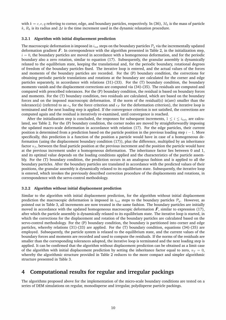
3.2.1 Algorithm with initial displacement prediction

The macroscopic deformation is imposed in itot steps on the boundary particles Pq via the incrementally updateddeformation gradient F . In correspondence with the algorithm presented in Table 2, in the initialization step,i = 0, the boundary particles are moved in accordance with a homogeneous deformation, and for the periodicboundary also a zero rotation, similar to equation (17). Subsequently, the granular assembly is dynamicallyrelaxed to the equilibrium state, keeping the translational and, for the periodic boundary, rotational degreesof freedom of the boundary particles fixed. The iterative loop is entered, and the actual values of the forcesand moments of the boundary particles are recorded. For the (P) boundary condition, the corrections forobtaining periodic particle translations and rotations at the boundary are calculated for the corner and edgeparticles separately, in accordance with relations (31)-(33). For the (T) boundary condition, the boundarymoments vanish and the displacement corrections are computed via (34)-(35). The residuals are computed andcompared with prescribed tolerances. For the (P) boundary condition, the residual is based on boundary forcesand moments. For the (T) boundary condition, two residuals are calculated, which are based on the boundaryforces and on the imposed macroscopic deformation. If the norm of the residual(s) is(are) smaller than thetolerance(s) (referred to as εa for the force criterion and εF for the deformation criterion), the iterative loop isterminated and the next loading step is applied. If the convergence criterion is not satisfied, the corrections arecomputed again and the residual is iteratively re-examined, until convergence is reached.

After the initialization step is concluded, the responses for subsequent increments, 1 ≤ i ≤ itot, are calcu-lated, see Table 2. For the (P) boundary condition, the corner nodes are moved by straightforwardly imposingthe updated macro-scale deformation in accordance with relation (17). For the edge particles, their currentposition is determined from a prediction based on the particle position in the previous loading step i− 1. Morespecifically, this prediction is a function of the position a particle would have in case of a homogeneous de-formation (using the displacement boundary condition (17)), plus the difference, multiplied by an inheritancefactor nf , between the final particle position at the previous increment and the position the particle would haveat the previous increment under a homogeneous deformation. The inheritance factor lies between 0 and 1,and its optimal value depends on the loading conditions applied and the characteristics of the particle assem-bly. For the (T) boundary condition, the prediction occurs in an analogous fashion and is applied to all theboundary particles. After the boundary particles are translated in accordance with the predicted values of theirpositions, the granular assembly is dynamically relaxed to its equilibrium state. Subsequently, the iterative loopis entered, which invokes the previously described correction procedure of the displacements and rotations, incorrespondence with the servo-control methodology.

3.2.2 Algorithm without initial displacement prediction

Similar to the algorithm with initial displacement prediction, for the algorithm without initial displacementprediction the macroscopic deformation is imposed in itot steps to the boundary particles Pq. However, aspointed out in Table 3, all increments are now treated in the same fashion. The boundary particles are initiallymoved in accordance with the updated homogeneous macroscopic deformation F , similar to expression (17),after which the particle assembly is dynamically relaxed to its equilibrium state. The iterative loop is started, inwhich the corrections for the displacement and rotation of the boundary particles are calculated based on theservo-control methodology. For the (P) boundary condition, the boundary is partitioned into corner and edgeparticles, whereby relations (31)-(33) are applied. For the (T) boundary condition, equations (34)-(35) areemployed. Subsequently, the particle system is relaxed to the equilibrium state, and the current values of theboundary forces and moments are recorded and used to compute the residuals. If the norms of the residuals aresmaller than the corresponding tolerances adopted, the iterative loop is terminated and the next loading step isapplied. It can be confirmed that the algorithm without displacement prediction can be obtained as a limit caseof the algorithm with initial displacement prediction by setting the inheritance factor equal to zero, nf = 0,whereby the algorithmic structure provided in Table 2 reduces to the more compact and simpler algorithmicstructure presented in Table 3.

4 Computational results for regular and irregular packings

The algorithms proposed above for the implementation of the micro-scale boundary conditions are tested on aseries of DEM simulations on regular, monodisperse and irregular, polydisperse particle packings.

10

ALGORITHM WITH INITIAL DISPLACEMENT PREDICTION

1. Initialization DEM simulation. Increment i = 01.1 Initialize boundary conditions by applying updated macro-scale deformation homogeneously

1.1.A if (P) =⇒ xq = FXq and Qq = I for q = 1..., Q1.1.B if (T) =⇒ xq = FXq and mq = 0 for q = 1..., Q

1.2 Dynamic relaxation. Obtain boundary forces and moments.1.3 Update particle configuration

1.3.A if (P) =⇒ Partition the boundary into corner c and edge e particlesCalculate edge particles displacement ∆ue and rotation ∆θe corrections via (31)-(32)and corner particles rotation corrections ∆θc via (33)

1.3.B if (T) =⇒ Calculate boundary particles displacement correction ∆uq via (34)-(35)1.4 Dynamic relaxation. Obtain boundary forces and moments.1.5 Calculate residual(s)

1.5.A if (P) =⇒ ra =

√∑E/2e=1(∆ae ·∆ae/a2

e + (∆me/me)2) + (∆mc/mc)2

1.5.B if (T) =⇒ ra =√∑Q

q=1 ∆aq ·∆aq/a2q and rF =

√∑Qq=1 ∆F q ·∆F q/F 2

q

1.6 Check for convergence: ra ≤ εa for (P); ra ≤ εa and rF ≤ εF for (T)1.6.A if converged =⇒ Save current configuration and go to 21.6.B if not converged =⇒ Return to 1.3

2. Subsequent increments 1 ≤ i ≤ itot2.1 Apply updated boundary conditions

2.1.A if (P) =⇒Impose updated macro-scale deformation on corner nodes: xc = FXc and Qq = IPrediction of the positions of edge particles:

xie = xi,(D)e + nf

(xi−1e − x

i−1,(D)e

)for e = 1...E/2

with x(D)e = FXe and the inheritance factor 0 < nf ≤ 1

2.1.B if (T) =⇒Prediction of the positions of boundary particles:

xiq = xi,(D)q + nf

(xi−1q − x

i−1,(D)q

)for q = 1..., Q

with x(D)q = FXq and the inheritance factor 0 < nf ≤ 1

2.2 Translate particles according to predictions 2.1.A, or 2.1.B2.3 Dynamic relaxation. Obtain boundary forces and moments.2.4 Update particle configuration with displacement and rotation corrections ∆u and ∆θ

2.4.A if (P) =⇒ Refer to 1.3.A2.4.B if (T) =⇒ Refer to 1.3.B

2.5 Dynamic relaxation. Obtain boundary forces and moments.2.6 Calculate residual(s)

2.6.A if (P) =⇒ Refer to 1.5.A2.6.B if (T) =⇒ Refer to 1.5.B

2.7 Check for convergence: ra ≤ εa for (P); ra ≤ εa and rF ≤ εF for (T)2.7.A if converged =⇒ Save current configuration and go to 2 (next increment i+ 1)2.7.A if not converged =⇒ Return to 2.4

Table 2: Algorithm for the (P) and (T) boundary conditions with initial displacement prediction.

4.1 Regular monodisperse packing

In this section the responses of three different regular, monodisperse particle packings are considered, whichconsist of circular particles of radius R = 1.02 mm, where the centroids of two particles in contact initially areat a distance of 2.0 mm. The initial volumes of the packings are V = [64, 324, 784] mm2, which are calculatedfrom the locations of the centroids of the four corner particles. The number of particles of the three prackingsare equal to np = [25, 100, 225]. The particle volume fraction related to initial volume occupied by the innerparticles is v = 0.785. The corresponding coordination number, which reflects the average number of contactsof the inner particles, equals 4.

11

ALGORITHM WITHOUT INITIAL DISPLACEMENT PREDICTION

1. DEM simulation. Increments 0 ≤ i ≤ itot1.1 Initialize boundary conditions by applying updated macro-scale deformation homogeneously

1.1.A if (P) =⇒ xq = FXq and Qq = I for q = 1..., Q1.1.B if (T) =⇒ xq = FXq and mq = 0 for q = 1..., Q

1.2 Dynamic relaxation. Obtain boundary forces and moments.1.3 Update particle configuration

1.3.A if (P) =⇒ Partition the boundary into corner c and edge e particlesCalculate edge particles displacement ∆ue and rotation ∆θe corrections via (31)-(32)and corner particles rotation corrections ∆θc via (33)

1.3.B if (T) =⇒ Calculate boundary particles displacement correction ∆uq via (34)-(35)1.4 Dynamic relaxation. Obtain boundary forces and moments.1.5 Calculate residual(s)

1.5.A if (P) =⇒ ra =

√∑E/2e=1(∆ae ·∆ae/a2

e + (∆me/me)2) + (∆mc/mc)2

1.5.B if (T) =⇒ ra =√∑Q

q=1 ∆aq ·∆aq/a2q and rF =

√∑Qq=1 ∆F q ·∆F q/F 2

q

1.6 Check for convergence: ra ≤ εa for (P); ra ≤ εa and rF ≤ εF for (T)1.6.A if converged =⇒ Save current configuration and go to 1 (next increment i+ 1)1.6.B if not converged =⇒ Return to 1.3

Table 3: Algorithm for the (P) and (T) boundary conditions without initial displacement prediction.

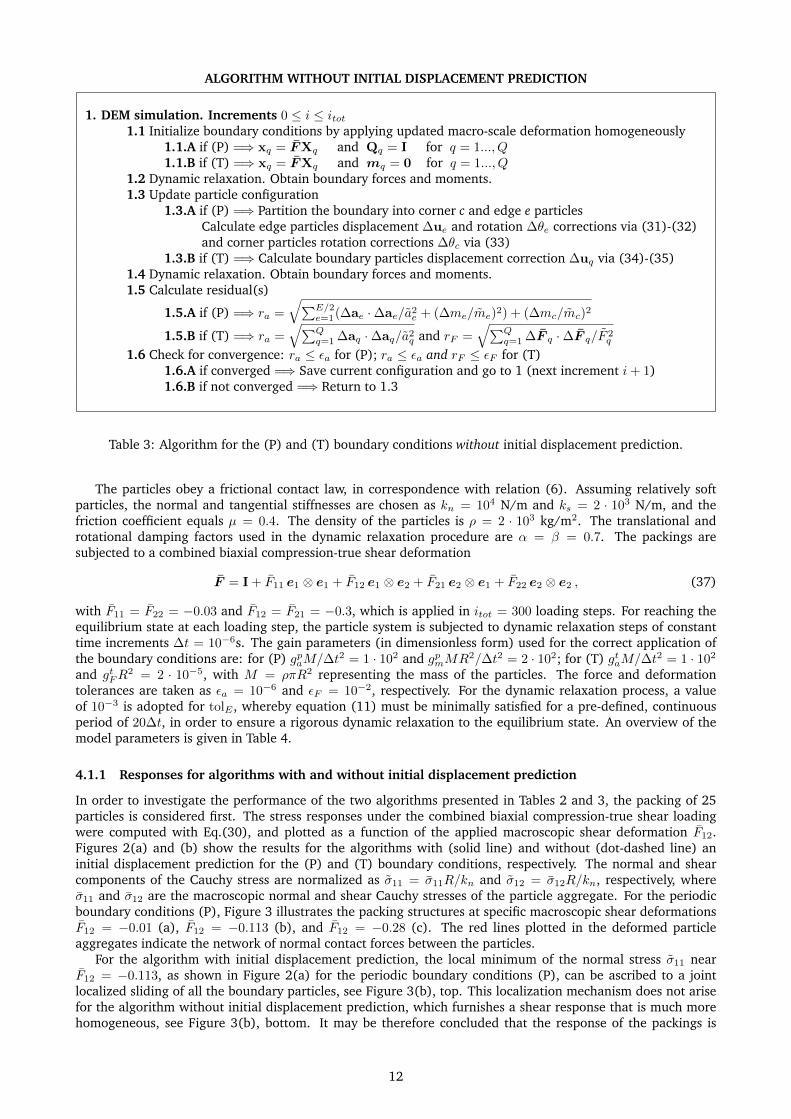
The particles obey a frictional contact law, in correspondence with relation (6). Assuming relatively softparticles, the normal and tangential stiffnesses are chosen as kn = 104 N/m and ks = 2 · 103 N/m, and thefriction coefficient equals µ = 0.4. The density of the particles is ρ = 2 · 103 kg/m2. The translational androtational damping factors used in the dynamic relaxation procedure are α = β = 0.7. The packings aresubjected to a combined biaxial compression-true shear deformation

F = I + F11 e1 ⊗ e1 + F12 e1 ⊗ e2 + F21 e2 ⊗ e1 + F22 e2 ⊗ e2 , (37)

with F11 = F22 = −0.03 and F12 = F21 = −0.3, which is applied in itot = 300 loading steps. For reaching theequilibrium state at each loading step, the particle system is subjected to dynamic relaxation steps of constanttime increments ∆t = 10−6s. The gain parameters (in dimensionless form) used for the correct application ofthe boundary conditions are: for (P) gpaM/∆t2 = 1 · 102 and gpmMR2/∆t2 = 2 · 102; for (T) gtaM/∆t2 = 1 · 102

and gtFR2 = 2 · 10−5, with M = ρπR2 representing the mass of the particles. The force and deformation

tolerances are taken as εa = 10−6 and εF = 10−2, respectively. For the dynamic relaxation process, a valueof 10−3 is adopted for tolE , whereby equation (11) must be minimally satisfied for a pre-defined, continuousperiod of 20∆t, in order to ensure a rigorous dynamic relaxation to the equilibrium state. An overview of themodel parameters is given in Table 4.

4.1.1 Responses for algorithms with and without initial displacement prediction

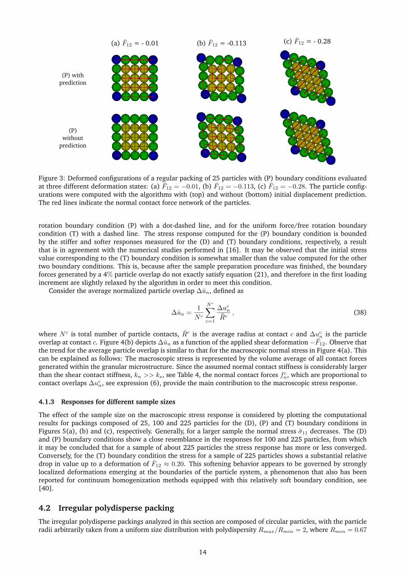
In order to investigate the performance of the two algorithms presented in Tables 2 and 3, the packing of 25particles is considered first. The stress responses under the combined biaxial compression-true shear loadingwere computed with Eq.(30), and plotted as a function of the applied macroscopic shear deformation F12.Figures 2(a) and (b) show the results for the algorithms with (solid line) and without (dot-dashed line) aninitial displacement prediction for the (P) and (T) boundary conditions, respectively. The normal and shearcomponents of the Cauchy stress are normalized as σ11 = σ11R/kn and σ12 = σ12R/kn, respectively, whereσ11 and σ12 are the macroscopic normal and shear Cauchy stresses of the particle aggregate. For the periodicboundary conditions (P), Figure 3 illustrates the packing structures at specific macroscopic shear deformationsF12 = −0.01 (a), F12 = −0.113 (b), and F12 = −0.28 (c). The red lines plotted in the deformed particleaggregates indicate the network of normal contact forces between the particles.

For the algorithm with initial displacement prediction, the local minimum of the normal stress σ11 nearF12 = −0.113, as shown in Figure 2(a) for the periodic boundary conditions (P), can be ascribed to a jointlocalized sliding of all the boundary particles, see Figure 3(b), top. This localization mechanism does not arisefor the algorithm without initial displacement prediction, which furnishes a shear response that is much morehomogeneous, see Figure 3(b), bottom. It may be therefore concluded that the response of the packings is

12

Parameter Value UnitElastic normal stiffness kn 1 · 104 N/mElastic tangential stiffness ks 2 · 103 N/mFriction coefficient µ 0.4 -Density ρ 2 · 103 kg/m2

Translational damping α 0.7 -Rotational damping β 0.7 -Time increment ∆t 10−6 sTolerance force (P), (T) εa 10−6 -Tolerance deformation (T) εF 10−2 -Gain force (P) gpaM/∆t2 1 · 102 -Gain moment (P) gpmMR2/∆t2 2 · 102 -Gain force (T) gtaM/∆t2 1 · 102 -Gain deformation (T) gtFR

2 2 · 10−5 -Tolerance dynamic relaxation tolE 10−3 -

Table 4: Physical and algorithmic model parameters.

rather sensitive to bifurcations in the equilibrium path followed, which here become evident due to the rela-tively low number of particles present in the packing. Under continuing deformation towards F12 = −0.28,the inner particles of the aggregate also develop substantial sliding, such that for both algorithms the particlestructure gradually reaches its densest packing structure, at which the deformation as well as the normal contactforce network become strongly homogeneous. Both for the normal and shear stress components the responsescomputed by the two algorithms at this stage have coalesced, and steadily grow under further increasing defor-mation.

A similar trend can be observed for the normal and shear stress responses of the particle aggregates with the(T) boundary condition, see Figure 2(b). The discrepancies in the responses computed by the two algorithmsappears to be less than for the (P) boundary condition. Since the computational robustness and efficiencyof the two algorithms is comparable in the present simulations, no clear distinction can be made in terms oftheir overall performance. Hence, as an arbitrary choice, the forthcoming DEM results are computed with thealgorithm without initial displacement prediction.

0 0.1 0.2 0.3

−F12

-0.025

0

0.025

0.05

−σ11,−σ12

−σ12

−σ11

With prediction

Without prediction

0 0.1 0.2 0.3

−F12

-0.025

0

0.025

0.05

−σ11,−σ12

−σ12

−σ11

With prediction

Without prediction

(a) (P) boundary condition (b) (T) boundary condition

Figure 2: Normalized macroscopic Cauchy stresses −σ11 and −σ12 versus the shear deformation −F12 for (a)periodic displacement/periodic rotation boundary condition (P) and (b) uniform force/free rotation boundarycondition (T). The responses relate to a regular monodisperse packing of 25 particles, and were computed bythe algorithms with (solid line) and without (dot-dashed line) initial displacement predictions.

4.1.2 Responses for the (D), (P) and (T) boundary conditions

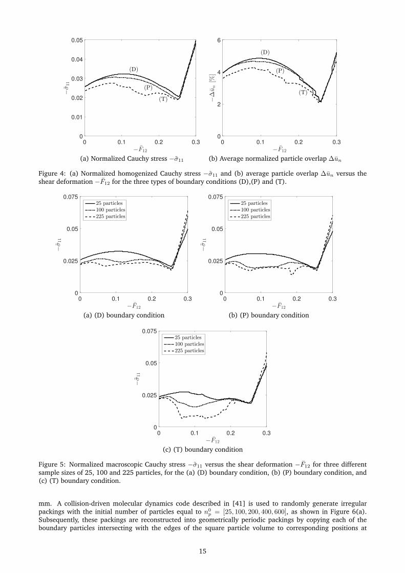
The influence of the choice of the boundary condition on the overall packing response is illustrated in Figure4(a). The (normalized) normal stress σ11 is shown as a function of the applied shear deformation F12 for thedisplacement/zero rotation boundary condition (D) with a solid line, for the periodic displacement/periodic

13

(a) F12 = - 0.01 (b) F12 = -0.113 (c) F12 = - 0.28

(P) withprediction

(P)without

prediction

Figure 3: Deformed configurations of a regular packing of 25 particles with (P) boundary conditions evaluatedat three different deformation states: (a) F12 = −0.01, (b) F12 = −0.113, (c) F12 = −0.28. The particle config-urations were computed with the algorithms with (top) and without (bottom) initial displacement prediction.The red lines indicate the normal contact force network of the particles.

rotation boundary condition (P) with a dot-dashed line, and for the uniform force/free rotation boundarycondition (T) with a dashed line. The stress response computed for the (P) boundary condition is boundedby the stiffer and softer responses measured for the (D) and (T) boundary conditions, respectively, a resultthat is in agreement with the numerical studies performed in [16]. It may be observed that the initial stressvalue corresponding to the (T) boundary condition is somewhat smaller than the value computed for the othertwo boundary conditions. This is, because after the sample preparation procedure was finished, the boundaryforces generated by a 4% particle overlap do not exactly satisfy equation (21), and therefore in the first loadingincrement are slightly relaxed by the algorithm in order to meet this condition.

Consider the average normalized particle overlap ∆un, defined as

∆un =1

N c

Nc∑

c=1

∆ucnRc

, (38)

where N c is total number of particle contacts, Rc is the average radius at contact c and ∆ucn is the particleoverlap at contact c. Figure 4(b) depicts ∆un as a function of the applied shear deformation −F12. Observe thatthe trend for the average particle overlap is similar to that for the macroscopic normal stress in Figure 4(a). Thiscan be explained as follows: The macroscopic stress is represented by the volume average of all contact forcesgenerated within the granular microstructure. Since the assumed normal contact stiffness is considerably largerthan the shear contact stiffness, kn >> ks, see Table 4, the normal contact forces f cn, which are proportional tocontact overlaps ∆ucn, see expression (6), provide the main contribution to the macroscopic stress response.

4.1.3 Responses for different sample sizes

The effect of the sample size on the macroscopic stress response is considered by plotting the computationalresults for packings composed of 25, 100 and 225 particles for the (D), (P) and (T) boundary conditions inFigures 5(a), (b) and (c), respectively. Generally, for a larger sample the normal stress σ11 decreases. The (D)and (P) boundary conditions show a close resemblance in the responses for 100 and 225 particles, from whichit may be concluded that for a sample of about 225 particles the stress response has more or less converged.Conversely, for the (T) boundary condition the stress for a sample of 225 particles shows a substantial relativedrop in value up to a deformation of F12 ≈ 0.20. This softening behavior appears to be governed by stronglylocalized deformations emerging at the boundaries of the particle system, a phenomenon that also has beenreported for continuum homogenization methods equipped with this relatively soft boundary condition, see[40].

4.2 Irregular polydisperse packing

The irregular polydisperse packings analyzed in this section are composed of circular particles, with the particleradii arbitrarily taken from a uniform size distribution with polydispersity Rmax/Rmin = 2, where Rmin = 0.67

14

0 0.1 0.2 0.3

−F12

0

0.01

0.02

0.03

0.04

0.05

−σ11

(T)

(P)

(D)

0 0.1 0.2 0.3

−F12

0

2

4

6

−∆un[%

]

(T)

(P)

(D)

(a) Normalized Cauchy stress −σ11 (b) Average normalized particle overlap ∆un

Figure 4: (a) Normalized homogenized Cauchy stress −σ11 and (b) average particle overlap ∆un versus theshear deformation −F12 for the three types of boundary conditions (D),(P) and (T).

0 0.1 0.2 0.3

−F12

0

0.025

0.05

0.075

−σ11

25 particles

100 particles

225 particles

0 0.1 0.2 0.3

−F12

0

0.025

0.05

0.075−σ11

25 particles

100 particles

225 particles

(a) (D) boundary condition (b) (P) boundary condition

0 0.1 0.2 0.3

−F12

0

0.025

0.05

0.075

−σ11

25 particles

100 particles

225 particles

(c) (T) boundary condition

Figure 5: Normalized macroscopic Cauchy stress −σ11 versus the shear deformation −F12 for three differentsample sizes of 25, 100 and 225 particles, for the (a) (D) boundary condition, (b) (P) boundary condition, and(c) (T) boundary condition.

mm. A collision-driven molecular dynamics code described in [41] is used to randomly generate irregularpackings with the initial number of particles equal to n0

p = [25, 100, 200, 400, 600], as shown in Figure 6(a).Subsequently, these packings are reconstructed into geometrically periodic packings by copying each of theboundary particles intersecting with the edges of the square particle volume to corresponding positions at

15

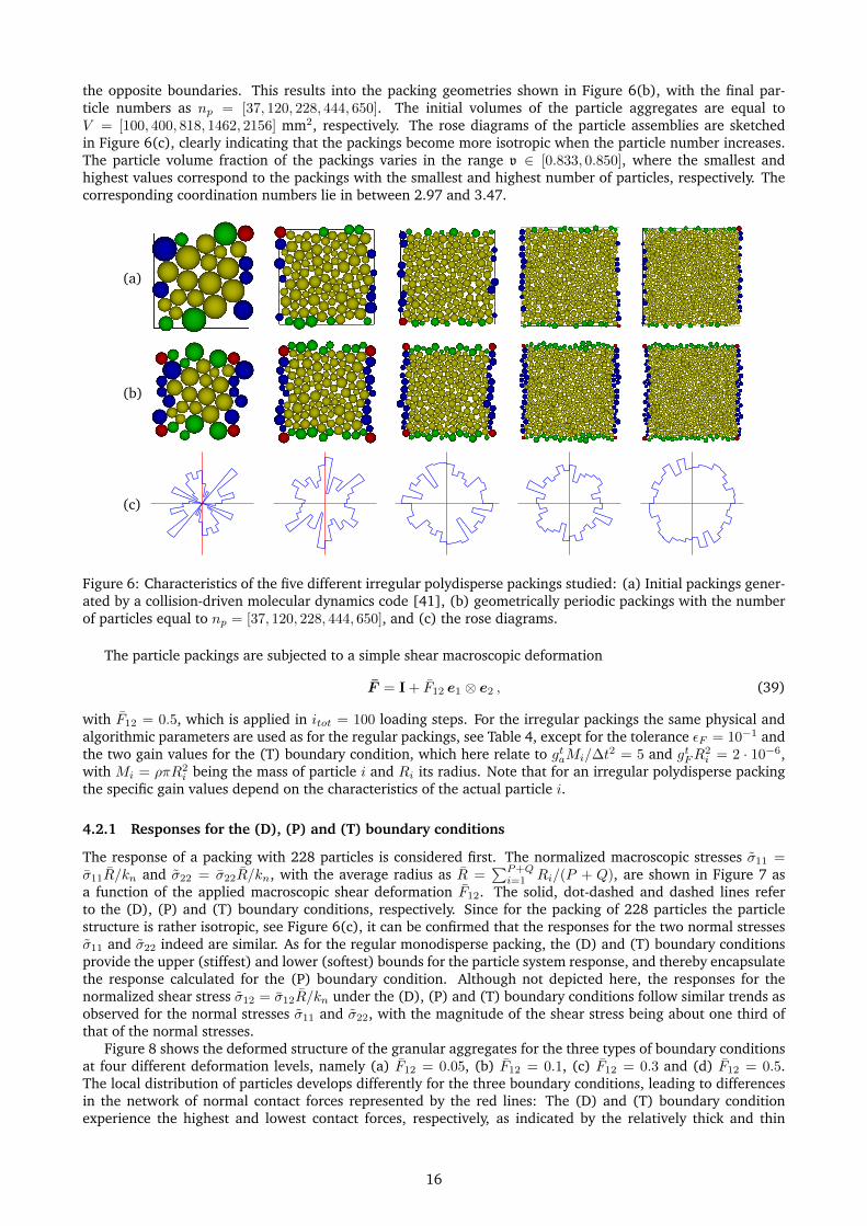
the opposite boundaries. This results into the packing geometries shown in Figure 6(b), with the final par-ticle numbers as np = [37, 120, 228, 444, 650]. The initial volumes of the particle aggregates are equal toV = [100, 400, 818, 1462, 2156] mm2, respectively. The rose diagrams of the particle assemblies are sketchedin Figure 6(c), clearly indicating that the packings become more isotropic when the particle number increases.The particle volume fraction of the packings varies in the range v ∈ [0.833, 0.850], where the smallest andhighest values correspond to the packings with the smallest and highest number of particles, respectively. Thecorresponding coordination numbers lie in between 2.97 and 3.47.

(a)

(b)

(c)

Figure 6: Characteristics of the five different irregular polydisperse packings studied: (a) Initial packings gener-ated by a collision-driven molecular dynamics code [41], (b) geometrically periodic packings with the numberof particles equal to np = [37, 120, 228, 444, 650], and (c) the rose diagrams.

The particle packings are subjected to a simple shear macroscopic deformation

F = I + F12 e1 ⊗ e2 , (39)

with F12 = 0.5, which is applied in itot = 100 loading steps. For the irregular packings the same physical andalgorithmic parameters are used as for the regular packings, see Table 4, except for the tolerance εF = 10−1 andthe two gain values for the (T) boundary condition, which here relate to gtaMi/∆t

2 = 5 and gtFR2i = 2 · 10−6,

with Mi = ρπR2i being the mass of particle i and Ri its radius. Note that for an irregular polydisperse packing

the specific gain values depend on the characteristics of the actual particle i.

4.2.1 Responses for the (D), (P) and (T) boundary conditions

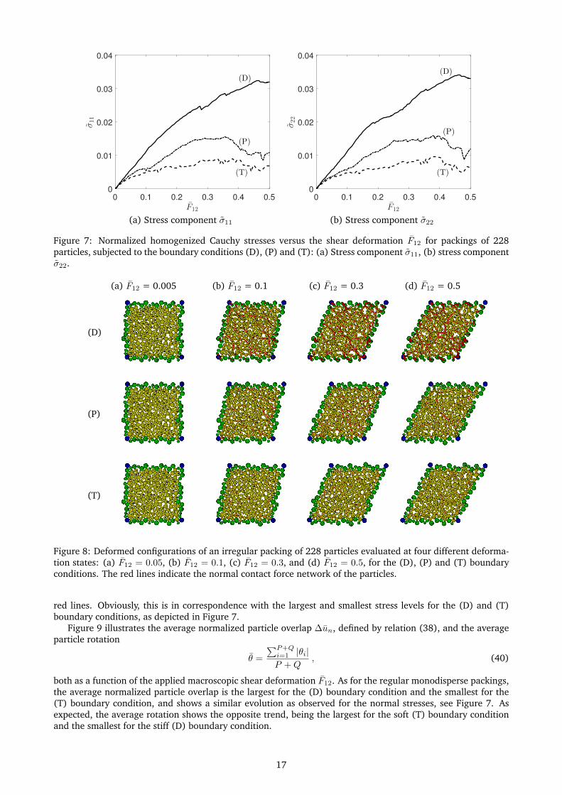
The response of a packing with 228 particles is considered first. The normalized macroscopic stresses σ11 =σ11R/kn and σ22 = σ22R/kn, with the average radius as R =

∑P+Qi=1 Ri/(P + Q), are shown in Figure 7 as

a function of the applied macroscopic shear deformation F12. The solid, dot-dashed and dashed lines referto the (D), (P) and (T) boundary conditions, respectively. Since for the packing of 228 particles the particlestructure is rather isotropic, see Figure 6(c), it can be confirmed that the responses for the two normal stressesσ11 and σ22 indeed are similar. As for the regular monodisperse packing, the (D) and (T) boundary conditionsprovide the upper (stiffest) and lower (softest) bounds for the particle system response, and thereby encapsulatethe response calculated for the (P) boundary condition. Although not depicted here, the responses for thenormalized shear stress σ12 = σ12R/kn under the (D), (P) and (T) boundary conditions follow similar trends asobserved for the normal stresses σ11 and σ22, with the magnitude of the shear stress being about one third ofthat of the normal stresses.

Figure 8 shows the deformed structure of the granular aggregates for the three types of boundary conditionsat four different deformation levels, namely (a) F12 = 0.05, (b) F12 = 0.1, (c) F12 = 0.3 and (d) F12 = 0.5.The local distribution of particles develops differently for the three boundary conditions, leading to differencesin the network of normal contact forces represented by the red lines: The (D) and (T) boundary conditionexperience the highest and lowest contact forces, respectively, as indicated by the relatively thick and thin

16

0 0.1 0.2 0.3 0.4 0.5

F12

0

0.01

0.02

0.03

0.04

σ11

(D)

(P)

(T)

0 0.1 0.2 0.3 0.4 0.5

F12

0

0.01

0.02

0.03

0.04

σ22

(D)

(P)

(T)

(a) Stress component σ11 (b) Stress component σ22

Figure 7: Normalized homogenized Cauchy stresses versus the shear deformation F12 for packings of 228particles, subjected to the boundary conditions (D), (P) and (T): (a) Stress component σ11, (b) stress componentσ22.

(a) F12 = 0.005 (b) F12 = 0.1 (c) F12 = 0.3 (d) F12 = 0.5

(D)

(P)

(T)

Figure 8: Deformed configurations of an irregular packing of 228 particles evaluated at four different deforma-tion states: (a) F12 = 0.05, (b) F12 = 0.1, (c) F12 = 0.3, and (d) F12 = 0.5, for the (D), (P) and (T) boundaryconditions. The red lines indicate the normal contact force network of the particles.

red lines. Obviously, this is in correspondence with the largest and smallest stress levels for the (D) and (T)boundary conditions, as depicted in Figure 7.

Figure 9 illustrates the average normalized particle overlap ∆un, defined by relation (38), and the averageparticle rotation

θ =

∑P+Qi=1 |θi|P +Q

, (40)

both as a function of the applied macroscopic shear deformation F12. As for the regular monodisperse packings,the average normalized particle overlap is the largest for the (D) boundary condition and the smallest for the(T) boundary condition, and shows a similar evolution as observed for the normal stresses, see Figure 7. Asexpected, the average rotation shows the opposite trend, being the largest for the soft (T) boundary conditionand the smallest for the stiff (D) boundary condition.

17

0 0.1 0.2 0.3 0.4 0.5

F12

0

2

4

6

8

∆un[%

]

(D)

(P)

(T)

0 0.1 0.2 0.3 0.4 0.5

F12

0

0.5

1

1.5

θ

(D)

(P)

(T)

(a) Particle overlap ∆un (b) Particle rotation θ

Figure 9: (a) Average normalized particle overlap ∆un and (b) average particle rotation θ versus the sheardeformation F12 for a packing of 228 particles subjected to the (D), (P) and (T) boundary conditions.

4.2.2 Convergence behavior of macroscopic response under increasing sample size

The convergence behavior of the apparent macroscopic response of the particle aggregate towards its effectiveresponse under increasing sample size is studied by subjecting the five microstructures depicted in Figure 6(b)to a simple shear deformation given by (39). In convergence studies, this type of loading condition occasionallyis characterized as “critical”, because of a relatively slow convergence behavior towards a representative vol-ume element (RVE). The convergence behavior is evaluated here by means of the L2-norm of the normalized,homogenized Cauchy stress tensor σ, integrated along the entire deformation path

‖σ‖L2=

( ∑

ij=11,22,12,21

∫ F12=0.5

F12=0

σ2ijdF12

)1/2

. (41)

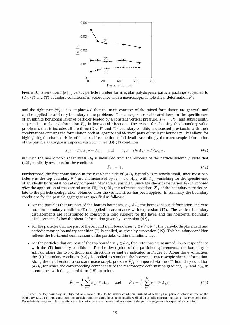
Figure 10 illustrates the stress norm‖σ‖L2as a function of the sample size, expressed in terms of the number of

particles. It can be observed that for the stiff (D) and soft (T) boundary conditions the stress norm, respectively,decreases and increases with increasing sample size, while for the periodic (P) boundary condition it remainsapproximately constant. These trends are typical for a change in apparent properties under increasing samplesize, see e.g., [21]. However, for arriving at an RVE the curves for the (D) (P) and (T) boundary conditionsmust coincide [31], which indeed is not the case for the largest sample of 650 particles. As already indicatedabove, the minimum size of the RVE depends on the type of loading condition applied, which is known to berelatively large under a macroscopic shear deformation. From the approximately constant stress value observedin Figure 10 for the (P) boundary condition, it may be expected that the stress response of the RVE will be closeto‖σ‖L2

≈ 0.011. Hence, in multi-scale simulations on granular materials, the computational costs can be keptmanageable by adopting the (P) boundary condition for a micro-structural sample of relatively small size, forwhich the homogenized response is similar to that of the minimal RVE with a much larger size.

5 Mixed boundary conditions

In this section the formulation and numerical implementation of mixed (D)-(P)-(T) boundary conditions is pre-sented. The homogenization framework proposed satisfies the Hill-Mandel micro-heterogeneity condition, andthus can be used for i) a consistent derivation of macro-scale constitutive relations from standard material testson particle aggregates subjected to any combination of (D)-, (P)- and/or (T)-type boundary conditions, andii) the efficient computation of the homogenized response of large-scale particle aggregates characterized by aspatial periodicity in one or two directions, i.e., granular layers exposed to uniform (D) and/or (T) boundaryconditions at their top and bottom surfaces. To the best of the authors’ knowledge, the formulation presentedis novel in the field of granular materials.

5.1 Formulation

For the formulation of the mixed boundary conditions, the basic particle configuration sketched in Figure 1is considered, with the boundary being split up into the top part ∂Vt, the bottom part ∂Vb, the left part ∂Vl

18

0 200 400 600 800

Particle number

0

0.01

0.02

0.03

0.04

‖σ‖L2

(D)

(P)

(T)

Figure 10: Stress norm ‖σ‖L2versus particle number for irregular polydisperse particle packings subjected to

(D), (P) and (T) boundary conditions, in accordance with a macroscopic simple shear deformation F12.

and the right part ∂Vr. It is emphasized that the main concepts of the mixed formulation are general, andcan be applied to arbitrary boundary value problems. The concepts are elaborated here for the specific caseof an infinite horizontal layer of particles loaded by a constant vertical pressure, P22 = P ∗22, and subsequentlysubjected to a shear deformation F12 in horizontal direction. The reason for choosing this boundary valueproblem is that it includes all the three (D), (P) and (T) boundary conditions discussed previously, with theircombinations entering the formulation both at separate and identical parts of the layer boundary. This allows forhighlighting the characteristics of the mixed formulation in full detail. Accordingly, the macroscopic deformationof the particle aggregate is imposed via a combined (D)-(T) condition

xq,1 = F12Xq,2 +Xq,1 and aq,2 = P21Aq,1 + P ∗22Aq,2 , (42)

in which the macroscopic shear stress P21 is measured from the response of the particle assembly. Note that(42)1 implicitly accounts for the condition

F11 = 1 . (43)

Furthermore, the first contribution in the right-hand side of (42)2 typically is relatively small, since most par-ticles q at the top boundary ∂Vt are characterized by Aq,1 << Aq,2, with Aq,1 vanishing for the specific caseof an ideally horizontal boundary composed of identical particles. Since the shear deformation F12 is imposedafter the application of the vertical stress P ∗22, in (42)1 the reference positions Xq of the boundary particles re-late to the particle configuration obtained after the vertical stress has been applied. In summary, the boundaryconditions for the particle aggregate are specified as follows:

• For the particles that are part of the bottom boundary, q ∈ ∂Vb, the homogeneous deformation and zerorotation boundary condition (D) is applied in accordance with expression (17). The vertical boundarydisplacements are constrained to construct a rigid support for the layer, and the horizontal boundarydisplacements follow the shear deformation given by expression (42)1.

• For the particles that are part of the left and right boundaries, q ∈ ∂Vl∪∂Vr, the periodic displacement andperiodic rotation boundary condition (P) is applied, as given by expression (19). This boundary conditionreflects the horizontal confinement of the particles within the infinite layer.

• For the particles that are part of the top boundary, q ∈ ∂Vt, free rotations are assumed, in correspondencewith the (T) boundary condition1. For the description of the particle displacements, the boundary issplit up along the two orthonormal directions e1 and e2 indicated in Figure 1. Along the e1-direction,the (D) boundary condition (42)1 is applied to simulate the horizontal macroscopic shear deformation.Along the e2-direction, a constant macroscopic pressure P ∗22 is imposed via the (T) boundary condition(42)2, for which the corresponding components of the macroscopic deformation gradient, F21 and F22, inaccordance with the general form (15), turn into

F21 =1

V

Q∑

q=1

xq,2 ⊗Aq,1 and F22 =1

V

Q∑

q=1

xq,2 ⊗Aq,2 . (44)

1Since the top boundary is subjected to a mixed (D)-(T) boundary condition, instead of leaving the particle rotations free at theboundary, i.e., a (T)-type condition, the particle rotations could have been equally well taken as fully constrained, i.e., a (D)-type condition.For relatively large samples the effect of this choice on the homogenized response of the particle aggregate is expected to be minor.

19

Note that the two deformation components above should be considered as a computational result obtainedby prescribing the stress component P ∗22.

The macroscopic deformation gradient F , which is followed by the four corner nodes of the sample, now is fullyspecified through its “(D)-type components” provided by (42)1 and (43), and its “(T)-type components” givenby (44)1,2. The corresponding macroscopic Piola-Kirchhoff stress tensor is defined by equation (23). For theadopted mixed-boundary conditions it will now be demonstrated that this stress definition satisfies the recastHill-Mandel condition given by expression (29), i.e., the energy consistency between the macro- and microscales. Accordingly, relation (29) is first split up with respect to the different boundary parts considered above,i.e., ∑

q∈∂Vb

(aq − P ·Aq

)· δwq +

∑

q∈∂Vl∪∂Vr

(aq − P ·Aq

)· δwq +

∑

q∈∂Vt

(aq − P ·Aq

)· δwq = 0 . (45)

For the bottom boundary ∂Vb, boundary condition (D) holds, which, by comparing equations (17) and (14),lets the micro-fluctuations of the displacements vanish, wq = 0. Hence, the first term in (45) is equal to zero.At the left and right boundaries q ∈ ∂Vl ∪ ∂Vr, the (P) boundary condition is imposed, for which the micro-fluctuations of the displacements are periodic, wl

q = wrq , see (14) and (19). Together with the anti-periodicity

of the boundary forces alq + arq = 0, see (20), the second term in (45) vanishes. Finally, for the top boundary∂Vt, the last term in (45) may be further developed as

∑

q∈∂Vt

[(aq,1 − P1jAq,j

)δwq,1 +

(aq,2 − P2jAq,j

)δwq,2

]= 0 . (46)

Along the e1-direction, the micro-fluctuations of the boundary particle displacements vanish, wq,1 = 0, incorrespondence with equation (42)1, by which the first term in (46) becomes zero. Along the e2-direction,the boundary forces are uniform, aq,2 − P2jAq,j = 0, see equation (42)2, so that the second term in (46)becomes zero. With this result, the Hill-Mandel condition (45) is proven to be satisfied for the mixed boundaryconditions.

5.2 Numerical implementation

The numerical algorithm for the implementation of the mixed boundary conditions is outlined in Table 5, and isbased on a combination of the algorithms presented in Section 3 for the (D), (P) and (T) boundary conditions,without an initial displacement prediction.

During stage 1 of the loading process, the vertical compressive stress P22 = P ∗22 is applied to the particleaggregate in a stepwise fashion2, using a total of ivs loading increments, with the subscript vs designating“vertical stress”. After initiating the displacement and rotation boundary conditions at the top ∂Vt and bottom∂Vb boundaries, the vertical stress is incrementally updated and subsequently used to compute the displacementand rotation corrections at the left and right boundaries with expressions (31)-(32), and the displacementcorrection at the top boundary boundary with

∆uq,2 = gta∆aq,2 with ∆aq,2 = aq,2 − P21Aq,1 − P ∗22Aq,2 . (47)

The expression above is derived from (42)2, whereby during the incremental application of the vertical stressP ∗22 the value of P21 is prescribed as zero, in order to avoid the initial development of a shear stress. After theparticle aggregate has reached its equilibrium state under dynamic relaxation, the boundary forces and momentsof the particles at the top, left and right boundaries are recorded and employed to compute the correspondingresiduals. When all residuals are lower than the prescribed values of the corresponding tolerances, the iterativeloop is stopped and the next vertical stress increment is applied. Otherwise, the iterative loop is entered again,until a converged solution is found. After the application of ivs increments the vertical stress has reached thedesired value, and stage 1 of the loading process has completed.

During stage 2 of the loading process, the horizontal shear deformation F12 is imposed on the particles at thetop ∂Vt and bottom ∂Vb boundaries of the granular assembly, by displacing these in a stepwise manner usingitot − ivs increments. The rotations of the particles at the top boundary are free, and the vertical displacementand rotation of the particles at the bottom boundary are fully constrained. In a similar way as explainedabove for stage 1, the boundary forces and moments in the relaxed equilibrium state are used to compute thedisplacement and rotation corrections at the periodic left and right boundaries ∂Vl and ∂Vr, and at the topboundary boundary ∂Vt. However, the only difference is that in (47) the shear stress P21 here is not prescribedas zero, but is calculated from the homogenized response of the particle assembly using equation (23). After the

2Instead of applying the vertical compressive stress by means of the first Piola-Kirchhoff stress P22, the Cauchy stress σ22 could havebeen used. The conversion of the Cauchy stress into the first Piola-Kirchhoff stress, which is the stress measure used in the numericalalgorithm presented in Table 5, can straightforwardly be accomplished by using the inverse form of expression (30).

20

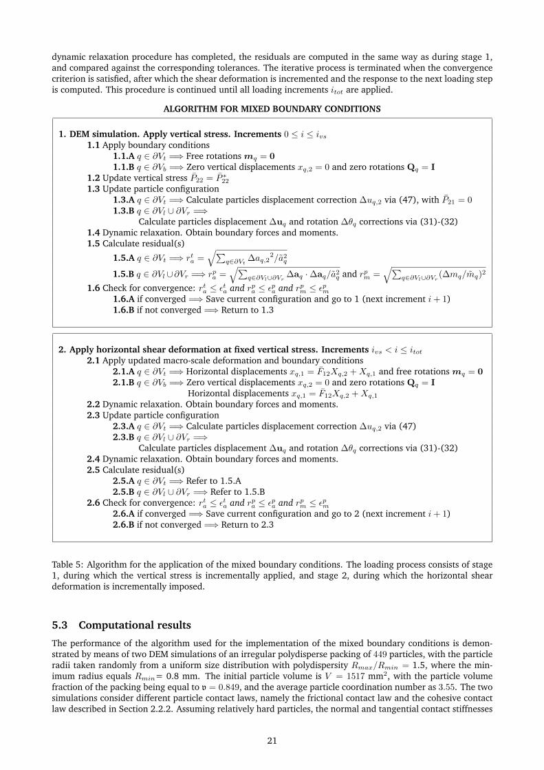
dynamic relaxation procedure has completed, the residuals are computed in the same way as during stage 1,and compared against the corresponding tolerances. The iterative process is terminated when the convergencecriterion is satisfied, after which the shear deformation is incremented and the response to the next loading stepis computed. This procedure is continued until all loading increments itot are applied.

ALGORITHM FOR MIXED BOUNDARY CONDITIONS

1. DEM simulation. Apply vertical stress. Increments 0 ≤ i ≤ ivs1.1 Apply boundary conditions

1.1.A q ∈ ∂Vt =⇒ Free rotations mq = 01.1.B q ∈ ∂Vb =⇒ Zero vertical displacements xq,2 = 0 and zero rotations Qq = I

1.2 Update vertical stress P22 = P ∗22

1.3 Update particle configuration1.3.A q ∈ ∂Vt =⇒ Calculate particles displacement correction ∆uq,2 via (47), with P21 = 01.3.B q ∈ ∂Vl ∪ ∂Vr =⇒

Calculate particles displacement ∆uq and rotation ∆θq corrections via (31)-(32)1.4 Dynamic relaxation. Obtain boundary forces and moments.1.5 Calculate residual(s)

1.5.A q ∈ ∂Vt =⇒ rta =√∑

q∈∂Vt∆aq,2

2/a2q

1.5.B q ∈ ∂Vl∪∂Vr =⇒ rpa =√∑

q∈∂Vl∪∂Vr∆aq ·∆aq/a2

q and rpm =√∑

q∈∂Vl∪∂Vr(∆mq/mq)2

1.6 Check for convergence: rta ≤ εta and rpa ≤ εpa and rpm ≤ εpm1.6.A if converged =⇒ Save current configuration and go to 1 (next increment i+ 1)1.6.B if not converged =⇒ Return to 1.3

2. Apply horizontal shear deformation at fixed vertical stress. Increments ivs < i ≤ itot2.1 Apply updated macro-scale deformation and boundary conditions

2.1.A q ∈ ∂Vt =⇒ Horizontal displacements xq,1 = F12Xq,2 +Xq,1 and free rotations mq = 02.1.B q ∈ ∂Vb =⇒ Zero vertical displacements xq,2 = 0 and zero rotations Qq = I

Horizontal displacements xq,1 = F12Xq,2 +Xq,1

2.2 Dynamic relaxation. Obtain boundary forces and moments.2.3 Update particle configuration

2.3.A q ∈ ∂Vt =⇒ Calculate particles displacement correction ∆uq,2 via (47)2.3.B q ∈ ∂Vl ∪ ∂Vr =⇒

Calculate particles displacement ∆uq and rotation ∆θq corrections via (31)-(32)2.4 Dynamic relaxation. Obtain boundary forces and moments.2.5 Calculate residual(s)

2.5.A q ∈ ∂Vt =⇒ Refer to 1.5.A2.5.B q ∈ ∂Vl ∪ ∂Vr =⇒ Refer to 1.5.B

2.6 Check for convergence: rta ≤ εta and rpa ≤ εpa and rpm ≤ εpm2.6.A if converged =⇒ Save current configuration and go to 2 (next increment i+ 1)2.6.B if not converged =⇒ Return to 2.3

Table 5: Algorithm for the application of the mixed boundary conditions. The loading process consists of stage1, during which the vertical stress is incrementally applied, and stage 2, during which the horizontal sheardeformation is incrementally imposed.

5.3 Computational results

The performance of the algorithm used for the implementation of the mixed boundary conditions is demon-strated by means of two DEM simulations of an irregular polydisperse packing of 449 particles, with the particleradii taken randomly from a uniform size distribution with polydispersity Rmax/Rmin = 1.5, where the min-imum radius equals Rmin= 0.8 mm. The initial particle volume is V = 1517 mm2, with the particle volumefraction of the packing being equal to v = 0.849, and the average particle coordination number as 3.55. The twosimulations consider different particle contact laws, namely the frictional contact law and the cohesive contactlaw described in Section 2.2.2. Assuming relatively hard particles, the normal and tangential contact stiffnesses

21

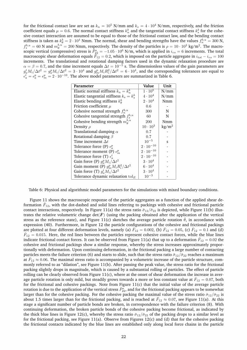
for the frictional contact law are set as kn = 105 N/mm and ks = 4 · 104 N/mm, respectively, and the frictioncoefficient equals µ = 0.6. The normal contact stiffness kbn and the tangential contact stiffness kbs for the cohe-sive contact interaction are assumed to be equal to those of the frictional contact law, and the bending contactstiffness is taken as kbθ = 2 · 104 Nmm. The normal, shear and bending strengths have the values f b,un = 300 N,f b,us = 60 N and mb,u

θ = 200 Nmm, respectively. The density of the particles is ρ = 10 · 103 kg/m2. The macro-scopic vertical (compressive) stress is P ∗22 = −1.05 · 106 N/m, which is applied in ivs = 6 increments. The totalmacroscopic shear deformation equals F12 = 0.2, which is imposed on the particle aggregate in itot − ivs = 100increments. The translational and rotational damping factors used in the dynamic relaxation procedure areα = β = 0.7, and the time increment equals ∆t = 10−5 s. The dimensionless values of the gain parameters aregtaMi/∆t

2 = gpaMi/∆t2 = 3 · 104 and gpmMiR

2i /∆t

2 = 6 · 104, and the corresponding tolerances are equal toεta = εpa = εpm = 2 · 10−10. The above model parameters are summarized in Table 6.

Parameter Value UnitElastic normal stiffness kn = kbn 1 · 105 N/mmElastic tangential stiffness ks = kbs 4 · 104 N/mmElastic bending stiffness kbθ 2 · 104 NmmFriction coefficient µ 0.6 -Cohesive normal strength f b,un 300 NCohesive tangential strength f b,us 60 NCohesive bending strength mb,u

θ 200 NmmDensity ρ 10 · 103 kg/m2

Translational damping α 0.7 -Rotational damping β 0.7 -Time increment ∆t 10−5 sTolerance force (P) εpa 2 · 10−10 -Tolerance moment (P) εpm 2 · 10−10 -Tolerance force (T) εta 2 · 10−10 -Gain force (P) gpaMi/∆t

2 3 · 104 -Gain moment (P) gpmMiR

2i /∆t

2 6 · 104 -Gain force (T) gtaMi/∆t

2 3 · 104 -Tolerance dynamic relaxation tolE 10−3 -

Table 6: Physical and algorithmic model parameters for the simulations with mixed boundary conditions.

Figure 11 shows the macroscopic response of the particle aggregates as a function of the applied shear de-formation F12, with the dot-dashed and solid lines referring to packings with cohesive and frictional particlecontact interactions, respectively. In Figure 11(a) the stress ratio σ12/σ22 is depicted, while Figure 11(b) illus-trates the relative volumetric change det(F ) (using the packing obtained after the application of the verticalstress as the reference state), and Figure 11(c) sketches the average particle rotation θ, in accordance withexpression (40). Furthermore, in Figure 12 the particle configurations of the cohesive and frictional packingsare plotted at four different deformation levels, namely (a) F12 = 0.002, (b) F12 = 0.05, (c) F12 = 0.1 and (d)F12 = 0.015. Here, the red lines between the particles represent cohesive contact forces, while the blue linesindicate frictional contact forces. It can be observed from Figure 11(a) that up to a deformation F12 = 0.02 thecohesive and frictional packings show a similar response, whereby the stress increases approximately propor-tionally with deformation. Upon continuing deformation, in the frictional packing a large number of contactingparticles meets the failure criterion (6) and starts to slide, such that the stress ratio σ12/σ22 reaches a maximumat F12 ≈ 0.06. The maximal stress ratio is accompanied by a volumetric increase of the particle structure, com-monly referred to as “dilation”, see Figure 11(b). After passing the peak value, the stress ratio for the frictionalpacking slightly drops in magnitude, which is caused by a substantial rolling of particles. The effect of particlerolling can be clearly observed from Figure 11(c), where at the onset of shear deformation the increase in aver-age particle rotation is only mild, but steadily grows towards a more or less constant value at F12 = 0.07, bothfor the frictional and cohesive packings. Note from Figure 11(c) that the initial value of the average particlerotation is due to the application of the vertical stress P ∗22, and for the frictional packing appears to be somewhatlarger than for the cohesive packing. For the cohesive packing the maximal value of the stress ratio σ12/σ22 isabout 1.5 times larger than for the frictional packing, and is reached at F12 ≈ 0.07, see Figure 11(a). At thisstage a significant number of particle bonds are broken, in correspondence with the failure criterion (8). Withcontinuing deformation, the broken particle bonds of the cohesive packing become frictional, as indicated bythe thick blue lines in Figure 12(c), whereby the stress ratio σ12/σ22 of the packing drops to a similar level asfor the frictional packing, see Figure 11(a). Observe from Figures 12(c) and (d) that for the cohesive packingthe frictional contacts indicated by the blue lines are established only along local force chains in the particle

22

structure, whereby the rest of the contacts remain cohesive, as indicated by the red lines. This implies that theoverall deformation of the packing towards the end of the loading process becomes governed by a localizedfailure zone, which indeed is associated to a strong softening behavior in the stress response, see Figure 11(a).Close to a shear deformation of F12 = 0.20, both the stress ratio σ12/σ22 and the relative volumetric changedet(F ) of the frictional and cohesive packings become approximately constant, characterizing the occurrence ofa so-called “critical state”. The overall residual strength at the critical state is σ12/σ22 ≈ 0.28. This value is onlyabout half of the value of 0.6 adopted for the local particle contact friction µ, which can be explained from thefact that at the end of the deformation process the dilating particle structure, instead of sliding, is predominatedby rolling of particles, see [7] for a more detailed discussion on this aspect.

As a final note, it is mentioned that the contact moments in the cohesive packing determine about 10% of thetotal potential energy. The reason that this contribution does not become manifest in the stress ratio σ12/σ22

depicted in Figure 11(a), is because the Cauchy stress is determined by contact forces only, see expressions(23) and (30). As already mentioned in Section 2.4, the overall effect by the contact moments on the particleaggregate can be accounted for through the introduction of a couple stress, but this stress measure is left out ofconsideration in the present study.

0 0.05 0.1 0.15 0.2

F12

0

0.2

0.4

0.6

σ12/σ22

Frictional

Cohesive

0 0.05 0.1 0.15 0.2

F12

0.975

1

1.025

1.05

det(F

)

FrictionalCohesive

(a) Stress ratio σ12/σ22 (b) Relative volumetric change det(F )

0 0.05 0.1 0.15 0.2

F12

0

0.2

0.4

0.6

θ

Frictional

Cohesive

(c) Average particle rotation θ

Figure 11: Macroscopic response of an infinite granular layer subjected to a vertical compressive stress P22 = P ∗22

and a horizontal shear deformation F12. (a) Stress ratio σ12/σ22, (b) relative volumetric change det(F ), and (c)average particle rotation θ, all plotted versus the applied shear deformation F12 for cohesive (dot-dashed line)and frictional (solid line) packings.

6 Conclusions

Novel numerical algorithms have been presented for the implementation of three types of classical boundaryconditions for a particle aggregate. The micro-scale boundary conditions are formulated within the discrete ele-ment method using large deformation theory, and, along the lines of [16], are imposed on a frame of boundaryparticles of the particle packing, in accordance with i) a homogeneous deformation and zero particle rotation

23

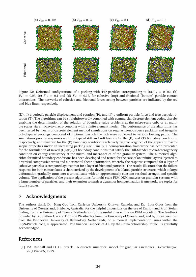
(a) F12 = 0.002 (b) F12 = 0.05 (c) F12 = 0.1 (d) F12 = 0.15

Coh

esiv

eFr

icti

onal

Figure 12: Deformed configurations of a packing with 449 particles corresponding to (a)F12 = 0.002, (b)F12 = 0.05, (c) F12 = 0.1 and (d) F12 = 0.15, for cohesive (top) and frictional (bottom) particle contactinteractions. The networks of cohesive and frictional forces acting between particles are indicated by the redand blue lines, respectively.

(D), ii) a periodic particle displacement and rotation (P), and iii) a uniform particle force and free particle ro-tation (T). The algorithms can be straightforwardly combined with commercial discrete element codes, therebyenabling the determination of the solution of boundary-value problems at the micro-scale only, or at multi-ple scales via a micro-to-macro coupling with a finite element model. The performance of the algorithms hasbeen tested by means of discrete element method simulations on regular monodisperse packings and irregularpolydisperse packings composed of frictional particles, which were subjected to various loading paths. Thesimulations provide responses with the typical stiff and soft bounds for the (D) and (T) boundary conditions,respectively, and illustrate for the (P) boundary condition a relatively fast convergence of the apparent macro-scopic properties under an increasing packing size. Finally, a homogenization framework has been presentedfor the formulation of mixed (D)-(P)-(T) boundary conditions that satisfy the Hill-Mandel micro-heterogeneitycondition on energy consistency at the micro- and macro-scales of the granular system. The numerical algo-rithm for mixed boundary conditions has been developed and tested for the case of an infinite layer subjected toa vertical compressive stress and a horizontal shear deformation, whereby the response computed for a layer ofcohesive particles is compared against that for a layer of frictional particles. The results illustrate that the failureresponse for both contact laws is characterized by the development of a dilated particle structure, which at largedeformation gradually turns into a critical state with an approximately constant residual strength and specificvolume. The application of the present algorithms for multi-scale FEM-DEM analyses on granular systems witha large number of particles, and their extension towards a dynamics homogenization framework, are topics forfuture studies.

7 Acknowledgments

The authors thank Dr. Ning Guo from Carleton University, Ottawa, Canada, and Dr. Lutz Gross from theUniversity of Queensland, Brisbane, Australia, for the helpful discussions on the use of Escript, and Prof. StefanLuding from the University of Twente, Netherlands for the useful interactions on DEM modeling. The feedbackprovided by Dr. Steffen Abe and Dr. Dion Weatherley from the University of Queensland, and by Joran Jessurunfrom the Eindhoven University of Technology, Netherlands, on numerical implementation issues within theESyS-Particle code, is appreciated. The financial support of J.L. by the China Scholarship Council is gratefullyacknowledged.

References

[1] P.A. Cundall and O.D.L. Strack. A discrete numerical model for granular assemblies. Geotechnique,29(1):47–65, 1979.

24

[2] H.J. Herrmann and S. Luding. Modeling granular media on the computer. Continuum Mechanics andThermodynamics, 10(4):189–231, 1998.

[3] F. Kun and H.J. Herrmann. A study of fragmentation processes using a discrete element method. ComputerMethods in Applied Mechanics and Engineering, 138(1):3 – 18, 1996.

[4] J.M. Ting, M. Khwaja, L.R. Meachum, and J.D. Rowell. An ellipse-based discrete element model for granu-lar materials. International Journal for Numerical and Analytical Methods in Geomechanics, 17(9):603–623,1993.

[5] R.I. Borja and J.R. Wren. Micromechanics of granular media. part I: Generation of overall constitu-tive equation for assemblies of circular disks. Computer Methods in Applied Mechanics and Engineering,127(1):13 – 36, 1995.

[6] K. Kaneko, K. Terada, T. Kyoya, and Y. Kishino. Global-local analysis of granular media in quasi-staticequilibrium. International Journal of Solids and Structures, 40(15):4043 – 4069, 2003.

[7] A.S.J. Suiker and N.A. Fleck. Frictional collapse of granular assemblies. Journal of Applied Mechanics,71(3):350–358, 2004.

[8] S. Luding. Micro-macro transition for anisotropic, frictional granular packings. International Journal ofSolids and Structures, 41:5821–5836, 2004.

[9] S. Luding and A.S.J. Suiker. Self-healing of damaged particulate materials through sintering. PhilosophicalMagazine, 88(28-29):3445–3457, 2008.

[10] A. Sing, V. Magnanimo, K. Saitoh, and S. Luding. Effect of cohesion on shear banding in quasistaticgranular materials. Physical Review E, 90(2), 022202, 2014.

[11] C. Wellmann, C. Lillie, and P. Wriggers. Homogenization of granular material modeled by a three-dimensional discrete element method. Computers and Geotechnics, 35(3):394 – 405, 2008.

[12] T.K. Nguyen, G. Combe, D. Caillerie, and J. Desrues. Modeling of cohesive granular materials by a multi-scale approach. In A. Yu, K. Dong, and S. Luding, editors, 7th International Conference on Micromechanicsof Granular Media (Powders and Grains), Sydney, Australia, volume 1542, pages 1194–1197, 2013.

[13] N. Guo and J. Zhao. A coupled FEM/DEM approach for hierarchical multiscale modelling of granularmedia. International Journal for Numerical Methods in Engineering, 99(11):789–818, 2014.

[14] G. Shahin, J. Desrues, S.D. Pont, G. Combe, and A. Argilaga. A study of the influence of rev variability indouble scale fem× dem analysis. International Journal for Numerical Methods in Engineering, 107(10):882–900, 2016.

[15] N. Guo and J. Zhao. Multiscale insights into classical geomechanics problems. International Journal forNumerical and Analytical Methods in Geomechanics, 2015.

[16] C. Miehe, J. Dettmar, and D. Zah. Homogenization and two-scale simulations of granular materials fordifferent microstructural constraints. International Journal for Numerical Methods in Engineering, 83(8-9):1206–1236, 2010.

[17] J.P. Dussault. Numerical stability and efficiency of penalty algorithms. SIAM Journal on Numerical Analysis,32:296–317, 1995.

[18] A. Gunaratne and Z. Wu. A penalty function method for constrained molecular dynamics simulation.International Journal of Numerical Analysis and Modeling, 8:496–517, 2011.

[19] K.J. Astrom and R.M. Murray. Feedback Systems: An Introduction for Scientists and Engineers. PrincetonUniversity Press, 2008.

[20] P.M. Suquet. Local and global aspects in the mathematical theory of plasticity. In A. Sawczuk andG. Bianchi, editors, Plasticity today: modelling, methods and applications, pages 279–310. Elsevier AppliedScience Publishers, London, 1985.

[21] V. Kouznetsova, W.A.M. Brekelmans, and F.P.T. Baaijens. An approach to micro-macro modeling of het-erogeneous materials. Computational Mechanics, 27(1):37–48, 2001.

[22] K. Terada, M. Hori, T. Kyoya, and N. Kikuchi. Simulation of the multi-scale convergence in computationalhomogenization approaches. International Journal of Solids and Structures, 37(16):2285 – 2311, 2000.

25

[23] C. Miehe, J. Schotte, and M. Lambrecht. Homogenization of inelastic solid materials at finite strains basedon incremental minimization principles. Application to the texture analysis of polycrystals. Journal of theMechanics and Physics of Solids, 50:2123–2167, 2002.

[24] C. Miehe and A. Koch. Computational micro-to-macro transitions of discretized microstructures undergo-ing small strains. Archive of Applied Mechanics, 72(4-5):300–317, 2002.

[25] J.P. Dettmar. Static and dynamic homogenization analyses of discrete granular and atomistic structures ondifferent time and length scales. PhD thesis, University of Stuttgart, 2006.

[26] Y. Wang and P. Mora. Modeling wing crack extension: Implications for the ingredients of discrete elementmodel. Pure and Applied Geophysics, 165(3-4):609–620, 2008.

[27] Y. Wang. A new algorithm to model the dynamics of 3-D bonded rigid bodies with rotations. Acta Geotech-nica, 4(2):117–127, 2009.

[28] D.O. Potyondy and P.A. Cundall. A bonded-particle model for rock. International Journal of Rock Mechanicsand Mining Sciences, 41(8):1329–1364, 2004.

[29] D. Weatherley, W. Hancock, V. Boros, and S. Abe. ESyS-Particle tutorial and user’s guide, version 2.3.1,2014.

[30] O.I. Imole, N. Kumar, V. Magnanimo, and S. Luding. Hydrostatic and shear behavior of frictionless granularassemblies under different deformation conditions. Kona Powder and Particle Journal, 30:84 – 108, 2013.

[31] R. Hill. Elastic properties of reinforced solids: some theoretical principles. Journal of the Mechanics andPhysics of Solids, 11(5):357–372, 1963.

[32] H.B. Muhlhaus and I. Vardoulakis. The thickness of shear bands in granular materials. Geotechnique,37(3):271–283, 1987.

[33] C.S. Chang and C.L. Liao. Constitutive relation for a particulate medium with the effect of particle rotation.International Journal of Solids and Structures, 26:437–453, 1990.

[34] C.S. Chang and L. Ma. Elastic material constants for isotropic granular solids with particle rotation.International Journal of Solids and Structures, 29:1001–1018, 1992.

[35] A.S.J. Suiker, R. de Borst, and C.S. Chang. Micro-mechanical modelling of granular material. Part 1:Derivation of a second-gradient micro-polar constitutive theory. Acta Mechanica, 149:161–180, 2001.

[36] A.S.J. Suiker, R. de Borst, and C.S. Chang. Micro-mechanical modelling of granular material. Part 2: Planewave propagation propagation in infinite media. Acta Mechanica, 149:181–200, 2001.

[37] A.S.J. Suiker and R. de Borst. Enhanced continua and discrete lattices for modelling granular assemblies.Philosophical Transactions of the Royal Society series A., 363:2543–2580, 2005.

[38] S. Virgo, S. Abe, and J.L. Urai. Extension fracture propagation in rocks with veins: Insight into thecrack-seal process using discrete element method modeling. Journal of Geophysical Research: Solid Earth,118(10):5236–5251, 2013.

[39] N. Guo and J. Zhao. The signature of shear-induced anisotropy in granular media. Computers and Geotech-nics, 47:1–15, 2013.

[40] E.W.C. Coenen, V.G. Kouznetsova, and M.G.D. Geers. Novel boundary conditions for strain localizationanalyses in microstructural volume elements. International Journal for Numerical Methods in Engineering,90(1):1–21, 2012.

[41] A. Donev, S. Torquato, and F.H. Stillinger. Neighbor list collision-driven molecular dynamics simulationfor nonspherical hard particles. I. algorithmic details. Journal of Computational Physics, 202(2):737–764,2005.

26