Department of Meteorology

Parallel Worlds with Extra Non-Hydrostaticness

Erin Thomson

A dissertation submitted in partial fulfilment of the requirement for the degree of MSc in Atmosphere, Oceans and Climate

August 2007

Acknowledgements

I would like to thank my supervisor Dr Robert Plant for all of his advice and support during

this project, and for performing all of the model runs for me. I would also like to thank Laura

Davies for pointing out a few silly mistakes I made when working with the model output, thus

preventing my nervous breakdown.

Thanks also go to my parents for supporting me throughout the course.

Abstract

Representation of cumulus convection in circulation models is an ongoing problem. The

traditional method is a parameterization, but this field is still far from providing an accurate

scheme with sensible assumptions. Cloud resolving models (CRMs) offer a more realistic

simulation of convective systems, but current computing capabilities prevent their use on a

global scale. There are various systems that have been suggested to allow the use of cloud

resolving models in a system covering the whole globe without requiring the computing

power needed to run a global CRM. One such approach, known as DARE, was proposed by

Kuang et al. (2005), in which the hydrostaticness of the system was reduced. Rescaling the

system to make it more non-hydrostatic increases the scale of convective cells, allowing them

to be resolved at resolutions more realistically computationally feasible.

Simulations using a CRM with a resolution of 2km were studied and compared to evaluate the

effects of the rescaling in both two and three dimensions. The effects noted were similar in

both dimensions, generally reducing the vertical velocities, increasing horizontal scales and

moistening the atmosphere. The effects of the rescaling on the differences caused by

dimensionality were also studied. The rescaling in general reduces the differences between

2D and 3D simulations, making 2D simulations in the rescaled system an attractive and

sensible prospect.

Contents

Acronyms and Abbreviations............................................................................................... i

1. Introduction ......................................................................................................................1

1.1 Importance of Convective Clouds on the Climate System ........................................1

1.2 Aims of the Project......................................................................................................1

2. The Interaction of Tropical Convection and Large Scale Dynamics..............................3

2.1 Introduction ................................................................................................................3

2.2 Influence of Large Scale Dynamics on Convection....................................................3

2.3 Effects of Convection on Large Scale Properties.......................................................5

3. Modelling The Interaction................................................................................................7

3.1 Introduction ................................................................................................................7

3.2 The Parameterization Problem ..................................................................................8

3.3 Cloud Resolving Models ...........................................................................................10

3.3.1 The Impact of Dimensionality on Cloud Resolving Models..............................13

3.4 Superparameterization .............................................................................................18

4. The Hypohydrostatic Approach.....................................................................................22

4.1 Introduction ..............................................................................................................22

4.1.1 Proof of Equivalency ..........................................................................................23

4.2 Implementing the Approach.....................................................................................27

4.3 Evaluation of the Approach......................................................................................28

4.3.1 Impact on Convective Scales..............................................................................28

4.3.2 Impacts on Large Scales ....................................................................................33

5. Model Setup ....................................................................................................................36

5.1 The Model .................................................................................................................36

5.2 Data Collected ...........................................................................................................38

6. Discussion of Experiments..............................................................................................41

6.1 Unconstrained Model Winds in Two Dimensions....................................................41

6.2 Applying the Hypohydrostatic Rescaling.................................................................50

6.2.1 In Two Dimensions.............................................................................................50

6.2.2 In Three Dimensions ..........................................................................................57

6.3 Comparing Two and Three Dimensions ..................................................................60

6.3.1 Without Rescaling ..............................................................................................60

6.3.2 With Rescaling ...................................................................................................63

6.4 Discussion ..................................................................................................................66

7. Conclusions .....................................................................................................................70

References ...........................................................................................................................72

Appendix: Implementation of Hypohydrostatic Rescaling in the Met Office LEM ........76

- i -

Acronyms and Abbreviations

2D Two-Dimensional

3D Three-Dimensional

ARM Atmospheric Radiation Measurement

CAPE Convective Available Potential Energy

CISK Conditional Instability of the Second Kind

COARE Coupled Ocean-Atmosphere Response Experiment

CRCP Cloud Resolving Convection Parameterization

CRM/CSRM Cloud/Cumulus (System) Resolving Model

DARE Diabatic Acceleration and Rescaling

DOE Department of Energy

GCM General Circulation Model

GCSS GEWEX Cloud Systems Study

GEWEX Global Energy and Water Cycle Experiment

LCL Lifting Condensation Level

LNB Level of Neutral Buoyancy

NWP Numerical Weather Prediction

PBL Planetary Boundary Layer

QBO Quasi-Biennial Oscillation

RAVE Reduced Acceleration in the Vertical

RCE Radiative-Convective Equilibrium

SCM Single Column Model

SGP Southern Great Plains

TOGA Tropical Ocean – Global Atmosphere

VME Vertical Momentum Equation

WISHE Wind-Induced Surface Heat Exchange

- 1 -

1. Introduction

1.1 Importance of Convective Clouds on the Climate System

Cumulus convection plays a very

important part in the atmospheric

circulation. Clouds and their

associated processes have

interactions with a number of

other processes in the climate

system, as illustrated in Figure

1.1. These feedbacks influence

the climate system in a number of

ways (Arakawa, 2004).

Convection also has an important

role in global atmospheric energy

transports, as while large scale

planetary circulations are

responsible for much of the

meridional energy transport, convective motions are responsible for most of the vertical

energy transport (Pauluis et al., 2006).

It is therefore very important that convective systems are accurately represented in climate

models. Unfortunately, the current representations of clouds account for a large fraction of the

errors in predicting climate variability (Randall et al., 2003b).

1.2 Aims of the Project

Representing convection explicitly in climate models is still computationally prohibitive, but

in 2005, Kuang et al. suggested a method to reduce the computational power needed while

allowing for convective systems to be resolved. A number of experiments have been carried

out to evaluate this approach, all of which have been performed in three dimensions. This

project aims to investigate the validity of this new approach when run in two dimensions, as

this is still more computationally cheap. The differences caused by dimensionality of the

Figure 1.1: Interaction between various processes in the climate system. Adapted from Arawaka (2004)

- 2 -

model when run conventionally and under the scheme of Kuang et al. will be compared, to

evaluate whether the changes made by the new approach improve or exacerbate the known

problems in two dimensions.

The next two chapters will discuss the interactions between convective systems and the large

scale environment, and current progress in their representations in numerical models. Chapter

4 will introduce the new approach and discuss previous experiments carried out with it. This

will be followed by a description of the model to be used in the project. Chapter 6 will then

contain a discussion of the experiments and comparisons carried out, and then finally a

summary of the important conclusions and suggestions for further work will be given in

chapter 7.

- 3 -

2. The Interaction of Tropical Convection and Large Scale

Dynamics

2.1 Introduction

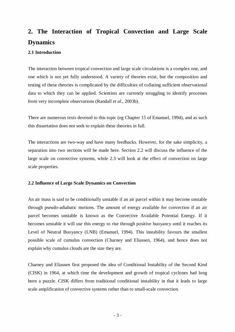
The interaction between tropical convection and large scale circulations is a complex one, and

one which is not yet fully understood. A variety of theories exist, but the composition and

testing of these theories is complicated by the difficulties of collating sufficient observational

data to which they can be applied. Scientists are currently struggling to identify processes

from very incomplete observations (Randall et al., 2003b).

There are numerous texts devoted to this topic (eg Chapter 15 of Emanuel, 1994), and as such

this dissertation does not seek to explain these theories in full.

The interactions are two-way and have many feedbacks. However, for the sake simplicity, a

separation into two sections will be made here. Section 2.2 will discuss the influence of the

large scale on convective systems, while 2.3 will look at the effect of convection on large

scale properties.

2.2 Influence of Large Scale Dynamics on Convection

An air mass is said to be conditionally unstable if an air parcel within it may become unstable

through pseudo-adiabatic motions. The amount of energy available for convection if an air

parcel becomes unstable is known as the Convective Available Potential Energy. If it

becomes unstable it will use this energy to rise through positive buoyancy until it reaches its

Level of Neutral Buoyancy (LNB) (Emanuel, 1994). This instability favours the smallest

possible scale of cumulus convection (Charney and Eliassen, 1964), and hence does not

explain why cumulus clouds are the size they are.

Charney and Eliassen first proposed the idea of Conditional Instability of the Second Kind

(CISK) in 1964, at which time the development and growth of tropical cyclones had long

been a puzzle. CISK differs from traditional conditional instability in that it leads to large

scale amplification of convective systems rather than to small-scale convection.

- 4 -

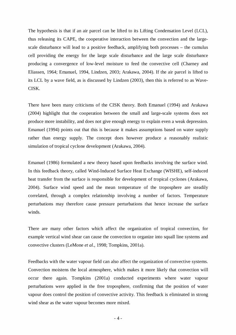
The hypothesis is that if an air parcel can be lifted to its Lifting Condensation Level (LCL),

thus releasing its CAPE, the cooperative interaction between the convection and the large-

scale disturbance will lead to a positive feedback, amplifying both processes – the cumulus

cell providing the energy for the large scale disturbance and the large scale disturbance

producing a convergence of low-level moisture to feed the convective cell (Charney and

Eliassen, 1964; Emanuel, 1994, Lindzen, 2003; Arakawa, 2004). If the air parcel is lifted to

its LCL by a wave field, as is discussed by Lindzen (2003), then this is referred to as Wave-

CISK.

There have been many criticisms of the CISK theory. Both Emanuel (1994) and Arakawa

(2004) highlight that the cooperation between the small and large-scale systems does not

produce more instability, and does not give enough energy to explain even a weak depression.

Emanuel (1994) points out that this is because it makes assumptions based on water supply

rather than energy supply. The concept does however produce a reasonably realistic

simulation of tropical cyclone development (Arakawa, 2004).

Emanuel (1986) formulated a new theory based upon feedbacks involving the surface wind.

In this feedback theory, called Wind-Induced Surface Heat Exchange (WISHE), self-induced

heat transfer from the surface is responsible for development of tropical cyclones (Arakawa,

2004). Surface wind speed and the mean temperature of the troposphere are steadily

correlated, through a complex relationship involving a number of factors. Temperature

perturbations may therefore cause pressure perturbations that hence increase the surface

winds.

There are many other factors which affect the organization of tropical convection, for

example vertical wind shear can cause the convection to organize into squall line systems and

convective clusters (LeMone et al., 1998; Tompkins, 2001a).

Feedbacks with the water vapour field can also affect the organization of convective systems.

Convection moistens the local atmosphere, which makes it more likely that convection will

occur there again. Tompkins (2001a) conducted experiments where water vapour

perturbations were applied in the free troposphere, confirming that the position of water

vapour does control the position of convective activity. This feedback is eliminated in strong

wind shear as the water vapour becomes more mixed.

- 5 -

While carrying out these experiments, Tompkins noticed that peak CAPE values were found

on the boundaries of the cold pools formed by the downdrafts of previous convective cells.

Upon further investigation, Tompkins (2001b) discovered that the spreading cold pool formed

as downdrafts inject cold, dry air into the Planetary Boundary Layer (PBL) is moister at its

boundaries and drier in the centre. These pools can trigger new daughter cells. This effect is

strongly related to the water vapour field.

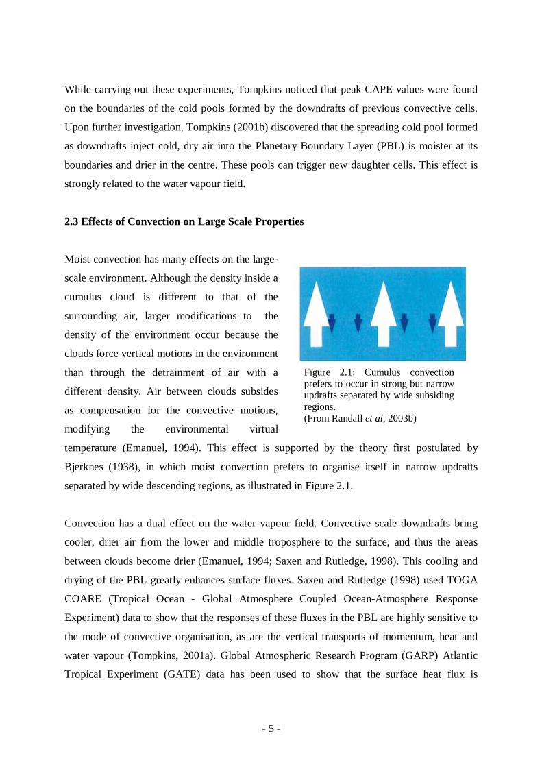
2.3 Effects of Convection on Large Scale Properties

Moist convection has many effects on the large-

scale environment. Although the density inside a

cumulus cloud is different to that of the

surrounding air, larger modifications to the

density of the environment occur because the

clouds force vertical motions in the environment

than through the detrainment of air with a

different density. Air between clouds subsides

as compensation for the convective motions,

modifying the environmental virtual

temperature (Emanuel, 1994). This effect is supported by the theory first postulated by

Bjerknes (1938), in which moist convection prefers to organise itself in narrow updrafts

separated by wide descending regions, as illustrated in Figure 2.1.

Convection has a dual effect on the water vapour field. Convective scale downdrafts bring

cooler, drier air from the lower and middle troposphere to the surface, and thus the areas

between clouds become drier (Emanuel, 1994; Saxen and Rutledge, 1998). This cooling and

drying of the PBL greatly enhances surface fluxes. Saxen and Rutledge (1998) used TOGA

COARE (Tropical Ocean - Global Atmosphere Coupled Ocean-Atmosphere Response

Experiment) data to show that the responses of these fluxes in the PBL are highly sensitive to

the mode of convective organisation, as are the vertical transports of momentum, heat and

water vapour (Tompkins, 2001a). Global Atmospheric Research Program (GARP) Atlantic

Tropical Experiment (GATE) data has been used to show that the surface heat flux is

Figure 2.1: Cumulus convection prefers to occur in strong but narrow updrafts separated by wide subsiding regions. (From Randall et al, 2003b)

- 6 -

especially increased in the region of the cold pool (Gaynor and Ropelewski, 1979; Johnson

and Nicholls, 1983).

As these effects change the large scale environment, they alter their own forcing, thus causing

complex feedbacks. There are many more effects in both directions, but this chapter

summarises some of the principal ones.

- 7 -

3. Modelling The Interaction

3.1 Introduction

Given our limited understanding of the mechanisms of the interactions discussed in the

previous chapter, it is unsurprising that modelling the situation is a problem. Modelling cloud

processes has a huge number of inherent uncertainties, some of which are illustrated in Figure

3.1. The vast scale differences between the various atmospheric systems that require

modelling also causes a problem when trying to create either a climate model or even a

numerical weather prediction (NWP) model in order for deep convection to be taken into

account.

General Circulation Models (GCMs), the primary atmospheric models used to simulate the

climate, are generally limited by computational resources to a resolution of the order of

100km, a scale much larger than the ~1km resolution that would be required to resolve

convective systems explicitly (Grabowski, 2001; Randall et al., 2003b; Pauluis et al., 2006;

Shutts and Palmer, 2007).

Instead, these models rely on parameterizations, the formulation of which is an ongoing

problem.

Figure 3.1: Cloud and associated processes for which major uncertainties in formulation exist. Adapted from Arakawa (2004).

- 8 -

3.2 The Parameterization Problem

A cloud parameterization is an idealized statistical or deterministic scheme designed to

represent the effects of the irresolvable clouds and their related small-scale systems on the

large scale atmospheric state using a set of semiempirical assumptions (Tiedtke, 1989;

Grabowski, 2001; Randall et al., 2003b; Kuang et al., 2005; Tomita et al., 2005; Pauluis and

Garner, 2006; Pauluis et al., 2006; Shutts and Palmer, 2007).

Research into cloud parameterizations began decades ago in the 1960s, and work on the

subject has remained intensive up to this day and will continue into the future. However,

despite this great accumulation of experience and many significant developments, the

progress made remains insufficient for its purpose (Randall et al., 2003b; Arakawa, 2004;

Kuang et al., 2005). As stated in Randall et al. (2003b), there is a reason that the

parameterization problem has yet to be solved: it is “very, very hard”; an appropriate set of

assumptions must be specified that reduce the real system with a huge number of dimensions

to a small number of equations (Arakawa, 2004).

Arakawa (2004) specifies a shortlist of important requirements that must be met to ensure the

validity of the principal closure, which links the overall properties and existence of cumulus

clouds to the large scale processes.

• The extent of the parameterizability of cumulus convection is unknown. The

hypotheses used to specify this should be logical and clearly stated.

• Balances in large-scale budgets should not be used as a closure. The prognostic

equations of a circulation model depend on the imbalances in these equations, and

therefore they cannot be assumed to balance for one part of the model and be

imbalanced for another. Only variables which are not predicted by the model may be

assumed to be at equilibrium.

• Cumulus convection is dependent on the buoyancy force, hence the parameterization

should be based on buoyancy.

When research into parameterization initially began, it was naively thought of as a much

simpler problem than it is now known to be, due to the more limited understanding at the time

of the complex nature of our atmosphere (Frank, 1983). The predecessors of many of the

parameterizations used in current climate models were constructed during these early years

- 9 -

(Arakawa, 2004). Among these were the parameterizations proposed by Manabe et al. (1965),

Kuo (1974) and Arakawa and Schubert (1974). Each was established from a very different set

of reasoning, yet the current schemes based upon them produce remarkably similar results

when applied to the same simulation (Arakawa, 2004).

The Manabe et al. scheme is among the earliest schemes formulated, and is one of the

simplest. In this scheme, if the air is supersaturated and conditionally unstable (Γ > Γm, where

Γ is the temperature lapse rate and Γm is the moist adiabatic lapse rate), moist convection is

assumed to occur. The profiles are then adjusted such that the air is saturated and neutrally

stable. While this scheme has many problems, not least of which that it requires

supersaturation on a grid-scale level for sub-grid scale convection to occur, it is a basis for

other, more complex, adjustment schemes developed later (Arakawa, 2004).

The Kuo scheme is a more complicated scheme based on the idea of CISK, considering a

convergence in the moisture budget, an approach which can be misleading (Arakawa, 2004).

This scheme has been subjected to tough criticism by Emanuel (1994) and Emanuel et al.

(1994), among others, on the basis that it assumes empirical agreements for which there is

little justification (Emanuel, 1994). Many later schemes, such as that proposed by Tiedtke

(1989) have been formulated with this scheme as a basis, and are intended to address such

issues.

The Arakawa-Schubert scheme introduces a quantity, A, the cloud-work function. A precise

definition of this quantity is given in Arakawa and Schubert (1974), but it can be considered

to be a measure of the moist-convective instability. It is assumed that if this is positive,

convective activity will occur. A = 0 represents a quasi-equilibrium state, to which the model

is adjusted if convection occurs. The specification of this quasi-equilibrium state is an issue

with this scheme (Emanuel, 1994; Arakawa, 2004). Many schemes have since been built upon

the foundations of this scheme. The assumption is that real convective systems respond

extremely quickly to changes in the large scale forcing; although the response time is usually

regarded as rapid, Cohen and Craig (2004) showed that it cannot be assumed to be

instantaneous. Betts (1986) and Emanuel (1991) incorporated a convective response time into

this scheme, introducing a relaxation timescale for the adjustment of the system to the quasi-

equilibrium.

- 10 -

All of these schemes have significant problems with their formulation, yet most do a

reasonable job of representing the effects of convection in models. Arakawa (2004) states that

we cannot keep relying on this kind of ‘luck’ when developing future schemes.

Another option is to avoid parameterizations completely, as discussed presently.

3.3 Cloud Resolving Models

In order to model convective clouds realistically, a much smaller grid size must be used than

that of a GCM. A Cloud Resolving Model (CRM, also known as a Cloud System Resolving

model or CSRM) represents moist cumulus convection explicitly rather than using a

parameterization, although cloud microphysics and other microprocesses are still represented

through parameterizations. CRMs usually have grid sizes of 2km or smaller, in line with

‘conventional’ wisdom that states this as the maximum resolution required to resolve

convection (Pauluis and Garner, 2006; Pauluis et al., 2006). Some sensitivity studies advise

that even grid sizes of this scale are too coarse, suggesting that resolutions of the order of

100m are required to properly simulate important cloud processes (Bryan et al., 2003; Petch,

2006).

CRMs have been used since the 1980s to evaluate the performance of cloud parameterizations

after the first CRM was developed by Yamazski in 1975 (Randall et al. 2003b). A CRM can

be used to create a simulated data set against which parameterizations can be tested, as they

can compute and output many quantities that are difficult to observe and record. Careful

analysis of these results can be used to develop and improve the parameterizations, although

this is not a simple process (Randall et al. 2003b; Moeng et al., 2004). The GEWEX (Global

Energy and Water Cycle Experiment) Cloud Systems Study (GCSS) was set up by K.

Browning and colleagues in the early 1990s to bring the parameterization and CRM

modelling communities together in order that they could more easily cooperate on this type of

venture and further research in both fields (Randall et al., 2003a).

When modelling deep convective clouds and their associated stratiform clouds, even without

tuning, CRMs uniformly give better results than Single Column Models (SCMs), which are

basically the column physics of GCMs, but considered in isolation (Randall et al, 2003a;

Randall et al, 2003b). Both models can be considered as representing a single grid column in

- 11 -

a GCM, with large scale processes imposed as boundary or initial conditions upon them.

(Randall et al., 2003a; Arakawa, 2004). These artificial boundary conditions should, as much

as possible, give the appearance that the CRM is running in the real atmosphere (Emanuel,

1994). This idea is taken further in the superparameterization approach discussed in the next

section. The superiority of CRMs is only to be expected, considering the vast differences in

formulation and the significantly greater computing time required to run them.

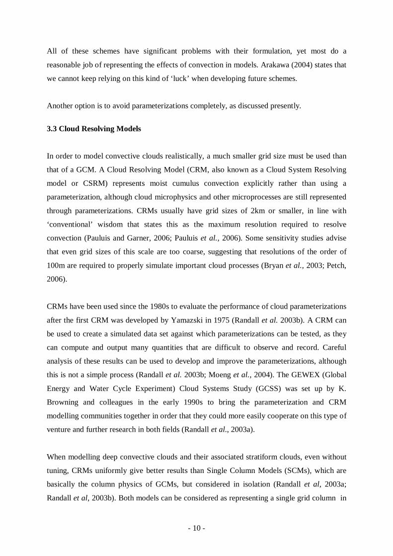
The GCSS tested several models of both kinds to actually demonstrate this fact. They

compared the outputs of these models with data from the US Department of Energy (DOE)

Atmospheric Radiation Measurement (ARM) Southern Great Plains (SGP) site in Oklahoma.

Figure 3.2 shows a selection of this data. The same results are found when using data from

other observational studies such as TOGA COARE (Randall et al, 2003a).

It can be seen that the CRM data is mostly in fairly good agreement with the observed data for

all three quantities, with the SCM outputs almost always producing worse results (Randall et

al. 2003a).

Considering the remarkably good results from CRMs, the ideal situation would be to perform

a global simulation using a CRM (Randall et al., 2003b). The computing power required to do

this, however, is immense, and almost all CRM simulations are run in a limited domain

(Emanuel, 1994; Peters and Bretherton, 2006)

Tomita et al. (2005) have performed some preliminary studies of a global 3D CRM with an

aqua-planet. Simulations were executed at resolutions of 14, 7 and 3.5km, with durations of

30, 30 and 10 days respectively. The 3.5 and 7km simulations in particular produced some

realistic features including a diurnal precipitation cycle and hierarchical cloud structures,

which were also captured in the 14km run. The higher resolution runs are likely the more

realistic.

- 12 -

Figure 3.2: A comparison of time-averaged C(S)RM and SCM results, based on data from the DOE ARM SGP site. (a) Water vapour, (b) Temperature and (c) Cloud occurrence. (a) and (b) are shown relative to observations for a single multiweek observing period. (c) is shown relative to three shorter observation periods. (a) and (b) are functions of pressure, (c) is a function of height. Taken from Randall et al. (2003a)

- 13 -

Computing limitations still prohibit the use of a global CRM for a simulation on climatic

timescales (Tompkins and Craig, 1998; Randall et al., 2003b; Kuang et al., 2005; Tomita et

al, 2005; Pauluis et al., 2006). Powerful enough machines may exist within the next few

decades to allow for this (Pauluis et al., 2006), but currently models must rely on

parameterizations or other methods to work around the cloud resolving issue (Peters and

Bretherton, 2006).

3.3.1 The Impact of Dimensionality on Cloud Resolving Models

Modelling in two dimensions is an attractive prospect computationally, as it naturally uses far

fewer resources to simulate the same time period, and until recently two-dimensional

simulations were the only way to carry out experiments with large computational domains

(Grabowski and Moncrieff, 2001). However, 2D modelling also has its drawbacks, as a two

dimensional model simply cannot capture all of the complexities of a three dimensional

system. Even cloud systems that are commonly described as two-dimensional, such as the

squall line, contain some three-dimensional dynamics, thus necessitating the use of a 3D

model to accurately represent cloud interactions (Tompkins and Craig, 1998). Using two-

dimensions is therefore a compromise between computational expense and accuracy in

representing the atmosphere (Moeng et al, 2004).

Various studies have been carried out to investigate the effects of modelling in 2D. Some of

these differences are discussed below.

Winds

An issue that affects all of the studies is the tendency for two dimensional models to create a

significant mean horizontal wind (Held et al, 1993; Tompkins, 2000). Figure 3.3 shows the

vertical profile of these winds in the simulations run by Tompkins (2000). The winds in the

corresponding three dimensional simulation remained weak and insignificant.

These winds have been compared to the Quasi-Biennial Oscillation (QBO) in the stratosphere

(Held et al., 1993). This ‘QBO-like oscillation’ generates a switch in direction of convective

propagation linked with a change in wind direction at lower levels, and is estimated to have a

period of around 6 x 106s or 70 days.

- 14 -

These wind shears have considerable effects on statistical properties of the system such as

temperature and cloud cover (Tompkins, 2000). To avoid the complications of this, most 2D

studies prescribe a wind profile to which the model profile is relaxed (Held et al., 1993;

Tompkins, 2000; Grabowski and Moncrieff, 2001).

Updrafts

Tao et al. (1987) discovered that the cloud updrafts and downdrafts were, on average, more

intense in their three-dimensional simulations than in two dimensions. They found, however,

that the differences between the statistical properties of clouds in identical large-scale

environments were limited by the organisation of the clouds into a line structure in the three-

Figure 3.3: One-day average mean horizontal mean winds at 10 day intervals through a 2D simulation by Tompkins (2000), in which the winds were unconstrained.

- 15 -

dimensional simulations. Tompkins (2000) and Tompkins and Craig (1998) attribute this

organisation to the large wind shear imposed on their experiments and the 2D nature of the

forcing.

Energy

Simulations carried out by Lipps and

Hemler (1986) revealed differences in

the volume-averaged kinetic energy (K)

between their 2 and 3 dimensional runs.

This can be seen in Figure 3.4, which

shows the time variation of K for their

experiments – A is run in 3D with a

domain size of 24km by 16km, B and C

are 2D with domain sizes of 32km and

64km respectively. This property was

also a concern in the simulations of

Moeng et al. (2004).

Thermodynamics

Running a pair of 900-point simulations, now with horizontal mean winds constrained to

vanish, Tompkins (2000) discovered that although the frequency of convection (taking

vertical velocities over a certain threshold to indicate convective activity) was similar, the 2D

run was rather drier and had a mean temperature at equilibrium several degrees warmer than

its 3D counterpart, as shown in Figure 3.5.

These differences were somewhat unexpected, as the mean winds in each run were

constrained identically to be zero, and the latent and sensible heat fluxes constrained to

balance the identical imposed forcing. However, the differences can be explained by the

larger horizontal wind perturbations in the 2D case. The energy balance between surface

fluxes and imposed radiative cooling has the result that an increase in surface winds means a

smaller difference between the temperature and moisture of the boundary layer air and the

Figure 3.4: Time variation of volume-mean kinetic energy for runs A-C in the experiments of Lipps and Helmer (1986).

- 16 -

surface (in this case a sea surface). This implies warmer, moister air in the boundary layer,

which is what is seen in the 2D case. The increased surface perturbation winds in two

dimensions occur as a direct result of the geometric restrictions.

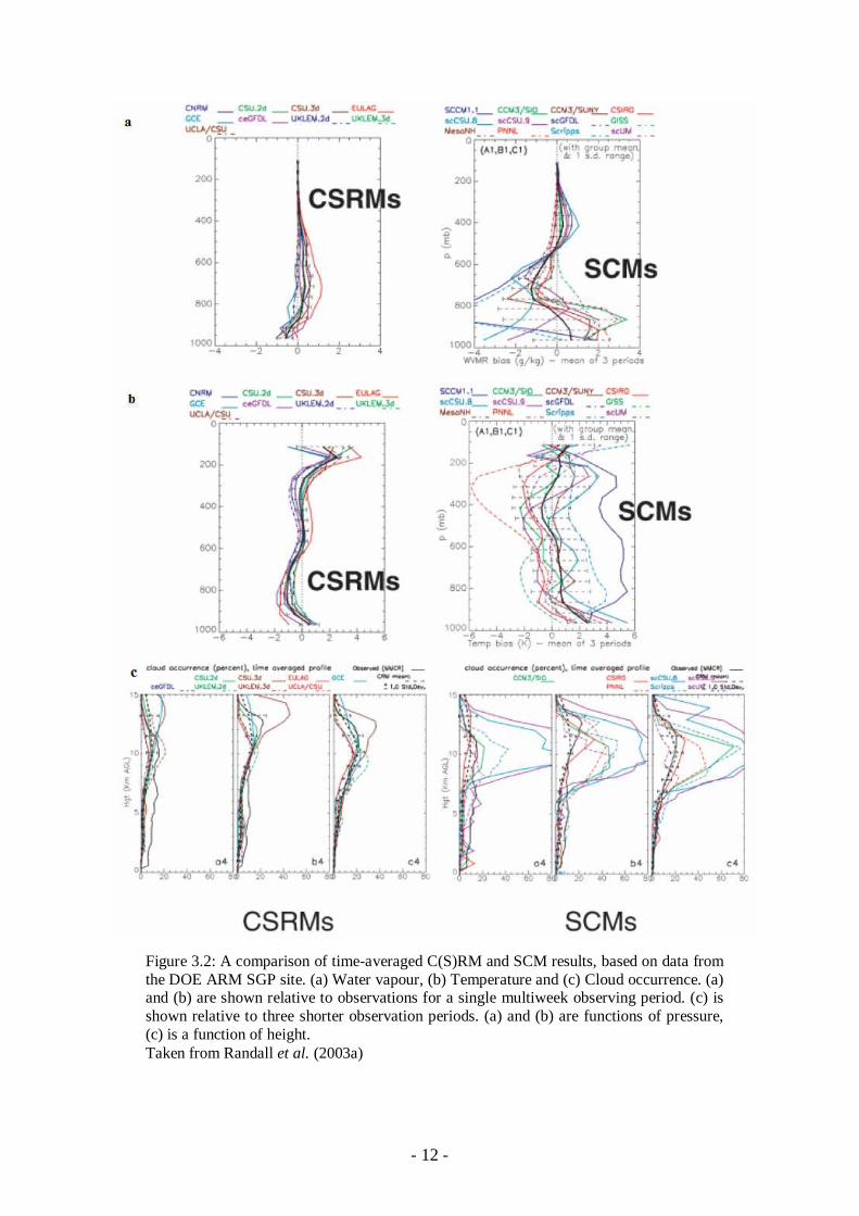
A convectively generated downdraft produces surface winds behind a gust front which

spreads outwards from the point of the convective activity, spreading out the downdraft air. In

three dimensions the velocity of these winds decreases as it spreads, due to the increasing

Figure 3.5: Time series of maximum vertical velocity (top), total column integrated water vapour (middle) and mean temperature (bottom) for 2D and 3D runs conducted by Tompkins (2000).

- 17 -

radius of the gust front, whereas in two dimensions the ‘radius’ of the spreading gust front

remains the same with increasing distance from the source, as illustrated by the schematic

diagram in Figure 3.6.

While the boundary layer is moister in two dimensions, the overall atmosphere is drier, which

does not appear to agree with the warmer temperatures. However, in two dimensions,

Tompkins noted that the convection appears to organise into bands, with no convection

occurring in some areas. The reason for these dry areas is unclear, but they appear to inhibit

any further convection from occurring in those areas, and those areas which are convective

become moister. These highly saturated areas are more likely to rain out, reducing the overall

water vapour content of the atmosphere (Tompkins, 2000).

Imposing a non-zero mean wind profile reduces the differences in the surface fluxes, therefore

also decreasing the differences in the temperature and moisture profiles (Tompkins, 2000).

The differences between 2D and 3D simulations are much reduced when a smaller 2D domain

is used. This is partly as a result of lower horizontal perturbation velocities, as the winds can

travel across the domain relatively quickly, and, due to the periodic boundary conditions,

meet and cancel each other out to some degree (Tompkins, 2000). The use of a smaller

domain also inhibits the organisation of the convective activity into clusters or other

structures.

Figure 3.6: Schematic of expected differences in surface winds between two and three dimensions. The arrows indicate surface winds and downdrafts, with thicker arrows representing stronger winds. Adapted from Tompkins (2000).

- 18 -

Two-dimensional simulations have also been utilised in the following unique approach to the

parameterization problem.

3.4 Superparameterization

Superparameterization, or Cloud Resolving Cumulus Parameterization (CRCP), is an

alternative approach to the problem of modelling cumulus convection that was suggested by

Grabowski (Grabowski and Smolarkiewicz, 1999; Grabowski, 2001) as a possible way out of

the parameterization ‘deadlock’. In this approach, several small-domain CRMs are used to

replace the traditional parameterizations of a GCM, with a single two dimensional CRM being

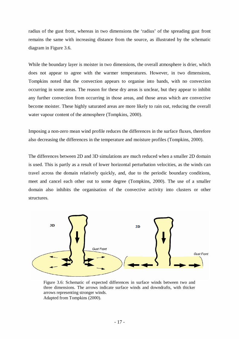
embedded into each grid box of the GCM, as illustrated in Figure 3.7 (a), and thus reducing

uncertainties in the ouput. (Tomita et al. 2005). The CRM has periodic horizontal boundary

conditions to maintain energy conservation (Grabowski and Smolarkiewicz, 1999) and does

not fill the GCM grid box, representing instead only a sample area of the box, which is

assumed to be statistically representative of the whole grid box (Randall et al., 2003b). At the

point of interaction between the GCM and the CRM, the GCM passes information about large

scale systems into the CRM, the CRM simulates the cloud system based on this information,

and, after using statistics to fill the grid box, passes the relevant information back to the GCM.

Grabowski and Smolarkiewicz (1999) ran a comparison of this method with a full 3D CRM in

a small domain of 400kmx400km. The ‘GCM’ ran with a horizontal grid length of 40km, and

the CRM with 2km. They discovered that the patterns of precipitation that developed in each

of the experiments were similar, as can be seen in Figure 3.8. There are some issues related to

this approach, however. The first of which is that, as in a traditional parameterization, cloud

systems that develop in one grid box cannot propagate into the next grid box, as the CRMs in

each of these boxes are not connected. A cloud system may appear to propagate, but this is

only due to the fact that the large scale information passed from the GCM can propagate

across grid boxes (Grabowski, 2001; Randall et al, 2003; Arakawa, 2004). Another issue is

caused by the CRM being two-dimensional, as there are many possible orientations of the

model within the three-dimensional GCM grid box. Different orientations, as one would

expect, result in different outputs (Randall et al, 2003b). The 2D CRM also, naturally, suffers

from the issues inherent with 2D modelling, as discussed in the previous section.

- 19 -

An improvement to this scheme was suggested in 2003 by Arakawa (Randall et al, 2003;

Arakawa, 2004), in which two CRMs are embedded in each grid box, as illustrated in Figure

3.7 (b). These two CRMs are orthogonal, interacting at a single grid point in the GCM grid

box. This alleviates the problem of orientation, and can be used to create a quasi-3D CRM

using interpolation. (Randall et al, 2003b; Arakawa, 2004). The CRM system is actually 3D

only at the points of interaction between the two high resolution models.

A further improvement is to extend the boundaries of the CRMs to the walls of the GCM grid

boxes. This system, shown in Figure 3.7 (c), allows the CRMs to interact directly, and

simulated cloud systems that develop in one grid box can therefore now propagate into the

Figure 3.7: Illustrations of CRCP/Superparameterization. The black boxes represent grid cells in the GCM, the red lines represent the 2D CRMs that are embedded within them. The GCM and the domain average of the CRM interact at the black dots. (a) A single CRM embedded in each grid box. The CRM does not reach the edges of the

GCM grid box. (b) Two perpendicular 2D CRMs are embedded in each box. They still do not reach the

edges of the GCM grid box. The two CRMs interact at the black dot, where they overlap. The CRM is 3D at this point.

(c) The CRMs now reach the edges of the GCM grid boxes, thus allowing them to interact with the CRMs in the neighbouring grid boxes, depicted by the blue arrows. The large-scale winds are predicted at the white circles.

Adapted from Randall et al. (2003b)

- 20 -

next (Randall et al, 2003b; Arakawa, 2004). Convergence to a global CRM can be achieved

using this arrangement as the resolution of the GCM is refined until only a single grid point of

CRM exists within each GCM grid box.

Until the resolutions of the two models are of the same order of magnitude, the problem of

artificially separating the cloud-scale and large-scale motions will remain an issue using the

CRCP method (Tomita at al., 2005).

A major downside to the CRCP/Superparameterization approach is the computing power

required to carry it out. Even with a simplified CRM and the arrangement illustrated in Figure

3.7 (a), a superparameterized simulation requires computer time of at least two to three orders

of magnitude more than one using a traditional parameterization (Arakawa, 2004). This

system is however “perfectly parallel”, and the number of GCM grid boxes can be increased

without increasing the run time if the number of processors are also increased proportionally

(Randall et al., 2003b). The system in Figure 3.7 (c) does not have this advantage, and would

Figure 3.8 Hovmöller diagrams of NS-averaged precipitation rate with the light and dark shading representing 0.2 and 1mm/h respectively. (a) CRCP experiment (b) 3D CRM experiment From Grabowski and Smolarkiewicz, (1999)

- 21 -

take yet longer to run. This should, however, be compared with the computational cost of

running a global CRM, which would be at least six orders of magnitude greater than a current

GCM (Randall et al., 2003b).

Another inventive approach to the parameterization problem, and the one on which this

dissertation concentrates, is discussed in the following chapter.

- 22 -

4. The Hypohydrostatic Approach

4.1 Introduction

In order to circumvent the representation problems caused by the scale difference, as

discussed in the previous chapter, Kuang et al. (2005) proposed a new method, in which this

scale difference was artificially reduced. They presented this under the acronym DARE,

standing for Diabatic Acceleration and REscaling. The application of DARE reduces both the

spatial and temporal scales of large scale circulations by making the radius of the Earth

smaller by some factor (often written as γ) and increasing its rotation rate by the same factor,

which is referred to by Kuang et al. (2005) as the DARE factor. The response time of the

convective systems is also shortened by this factor in order to maintain the interaction

mechanism between them and the large scale circulations. This is achieved by multiplying all

diabatic fluxes, microphysical process rates and precipitation fall velocities by the DARE

factor (Kuang et al., 2005; Peters and Bretherton, 2006). This approach has also been referred

to as the ‘small Earth’ approach (Garner et al. 2007), for obvious reasons.

Other interpretations suggested by Garner et al. (2007) and Pauluis et al. (2006) are the ‘deep

Earth’ system and the hypohydrostatic model, the latter of which is referred to by Kuang et al.

(2005) as RAVE (Reduced Acceleration in the VErtical). The ‘deep Earth’ approach involves

a reduction of the Earth’s gravitational acceleration, which increases the pressure scale height

and hence the depth of the atmosphere. In the hypohydrostatic or RAVE approach, vertical

accelerations are reduced via the multiplication of the Dw/Dt term in the vertical momentum

equation (VME) by a factor greater than one.

All of these systems are, despite their very different approaches to the problem,

mathematically equivalent (Pauluis et al., 2006; Garner et al., 2007), as is shown here using a

simple basic equation set.

- 23 -

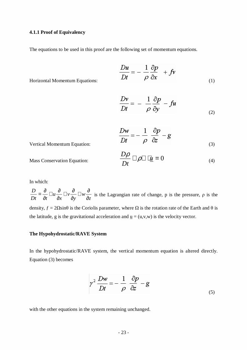
4.1.1 Proof of Equivalency

The equations to be used in this proof are the following set of momentum equations.

Horizontal Momentum Equations: (1)

(2)

Vertical Momentum Equation: (3)

Mass Conservation Equation: 0=⋅∇+ uDt

D ρρ (4)

In which:

zw

yv

xu

tDt

D

∂∂+

∂∂+

∂∂+

∂∂= is the Lagrangian rate of change, p is the pressure, ρ is the

density, ƒ = 2Ωsinθ is the Coriolis parameter, where Ω is the rotation rate of the Earth and θ is

the latitude, g is the gravitational acceleration and u = (u,v,w) is the velocity vector.

The Hypohydrostatic/RAVE System

In the hypohydrostatic/RAVE system, the vertical momentum equation is altered directly.

Equation (3) becomes

(5)

with the other equations in the system remaining unchanged.

- 24 -

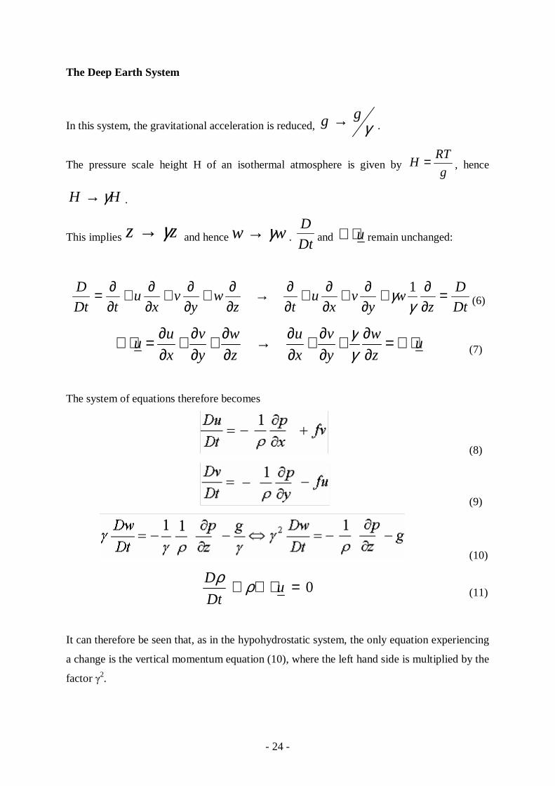
The Deep Earth System

In this system, the gravitational acceleration is reduced, γgg → .

The pressure scale height H of an isothermal atmosphere is given by g

RTH = , hence

HH γ→ .

This implies zz γ→ and hence ww γ→ . Dt

Dand u⋅∇ remain unchanged:

Dt

D

zw

yv

xu

tzw

yv

xu

tDt

D =∂∂+

∂∂+

∂∂+

∂∂→

∂∂+

∂∂+

∂∂+

∂∂=

γγ 1

(6)

uz

w

y

v

x

u

z

w

y

v

x

uu ⋅∇=

∂∂+

∂∂+

∂∂→

∂∂+

∂∂+

∂∂=⋅∇

γγ

(7)

The system of equations therefore becomes

(8)

(9)

(10)

0=⋅∇+ uDt

D ρρ (11)

It can therefore be seen that, as in the hypohydrostatic system, the only equation experiencing

a change is the vertical momentum equation (10), where the left hand side is multiplied by the

factor γ2.

- 25 -

The Small Earth/DARE System

This approach involves reducing the radius of the Earth and increasing its rotation rate:

Ω→Ω→ γγ ,aa . The reduction of the Earth’s radius reduces the horizontal scale in

all directions, and hence γxx → and γ

yy → . The increased rotation rate reduces the

length of a day and thus also the time scale, i.e. γtt → . The rotation rate also affects the

Coriolis parameter, ff γθγθ =Ω→Ω= sin2sin2 .

In this approach, Dt

Dand u⋅∇ are also affected as follows:

zw

yv

xu

tzw

yv

xu

tDt

D

∂∂+

∂∂+

∂∂+

∂∂→

∂∂+

∂∂+

∂∂+

∂∂= γγγ (12)

z

w

y

v

x

u

z

w

y

v

x

uu

∂∂+

∂∂+

∂∂→

∂∂+

∂∂+

∂∂=⋅∇ γγ (13)

These are not simple rescalings, and application of these in the mass conservation equation

reveals a problem, as shown below.

0≠

∂∂+

∂∂+

∂∂+

∂∂+

∂∂+

∂∂+

∂∂

→⋅∇+

z

w

y

v

x

u

zw

yv

xu

t

uDt

D

γγρρργργργ

ρρ

(14)

In order for the mass conservation equation to hold true, which it must always do, an

additional rescaling ww γ→ must be applied.

With the addition of this, the rescalings for Dt

Dand u⋅∇ are now:

Dt

D

zw

yv

xu

t

zw

yv

xu

tDt

D

γγγγγ =∂∂+

∂∂+

∂∂+

∂∂

→∂∂+

∂∂+

∂∂+

∂∂=

(15)

- 26 -

uz

w

y

v

x

u

z

w

y

v

x

uu ⋅∇=

∂∂+

∂∂+

∂∂→

∂∂+

∂∂+

∂∂=⋅∇ γγγγ (16)

The system of equations is therefore as follows:

(17)

(18)

(19)

000 =⋅∇+⇔

=⋅∇+⇔=⋅∇+ uDt

Du

Dt

Du

Dt

D ρρρργργργ (20)

Again, the only equation to undergo a change is the vertical momentum equation (19).

The three interpretations are hence mathematically equivalent.

In the DARE approach only, various parameters of the system must be rescaled to maintain

this equivalency, including the source terms for such quantities as θ. This is due to the

rescaling of the Dt

D term in this approach.

i.e. DtD

= S → DtD

= S etc. (21)

- 27 -

4.2 Implementing the Approach

From a modelling standpoint, the hypohydrostatic approach is the easiest interpretation to

introduce into a model, although its physical attributes are less clearly defined than in the

deep or small Earth analogues, as the γ2 factor needs only to be introduced in the Vertical

Momentum Equation. Scaling may also be required in the sub-grid scale viscosity to maintain

conservation of kinetic energy (Pauluis et al., 2006).

The idea of modifying the equations of motion to improve the performance of numerical

models is not new; it has been previously suggested as a method of improving computational

stability by reducing the hydrostatic-ness of fast inertia-gravity waves (Browning and Kreiss,

1986; Garner et al., 2007). It has not, however, previously been used as a method to assist in

the representation of convective dynamics, and no physical analogues were previously made

to these modified systems.

This approach is, of course, only useful if convection in the rescaled system responds to large-

scale forcing in a realistic manner, and if large scale dynamics are sufficiently unchanged as

to reliably represent the real atmosphere. Those large-scale motions which are in hydrostatic

balance are, naturally, unaffected directly by the rescaling as the term in the VME to be

multiplied is zero (Kuang et al., 2005). An assumption is also made that changing the scale

difference between the convective and large scale systems does not change their method of

interaction, as long as some difference in scale remains. Kuang et al (2005) liken this latter

assumption to the assumption that, with a sufficiently large Reynolds number, turbulent

behaviour is independent of viscosity. A difficulty with the approach is that timescales of

convective and large-scale motions are affected differently, and it is therefore impossible to

rescale microphysical processes consistently with both. As microphysics is important to

processes at both of these scales, this could cause an issue (Pauluis et al., 2006).

The initial assumptions must be tested through experimentation and comparison with

unscaled control model runs where possible.

- 28 -

4.3 Evaluation of the Approach

4.3.1 Impact on Convective Scales

Kuang et al. (2005) performed a comparison of an unscaled control CRM and a model run

with a DARE factor γ = 4, both run to Radiative-Convective Equilibrium (RCE – see Chapter

5 for more details about this). The model resolution remains the same, but the DARE run has

a domain smaller by a factor of 4 in both horizontal directions. They found that the

convection behaved similarly in both cases, and, as shown in Figure 4.1, that the domain

averaged temperature, cloud fraction and relative humidity profiles were a remarkably good

match.

The cloud fraction and relative humidity are slightly higher in the upper troposphere in the

DARE scaled run, due to the stronger updrafts required for the rescaling (w→γw), but the

differences are of a similar or smaller scale than the differences that can be caused by

microphysical uncertainties, so are not considered significant (Kuang et al., 2005).

As the DARE approach involves a rescaling of time, in order to compare the responses of

convection to a periodic large-scale forcing in the control and DARE runs, Kuang et al.

(2005) also had to rescale both the period of the forcing and its amplitude (Sθ(t)→ γSθ(t/γ), as

in equation 21). When the DARE results are scaled back for comparison, the two runs are

very similar in their responses, as shown in Figure 4.2.

DARE hence appears to faithfully simulate the convective activity which would appear in an

unscaled domain which is larger by a factor of γ, has the same grid size, and is run for a

period a factor of γ longer (Kuang et al., 2005; Peters and Bretherton, 2006).

Garner et al. (2007) performed simulations with a global coarse resolution model (grid lengths

of 2° latitude and 2.5° longitude) with very high values of the hypohydrostatic rescaling factor

(100, 200 and 300). They discovered that, even with these enormous rescalings, many features

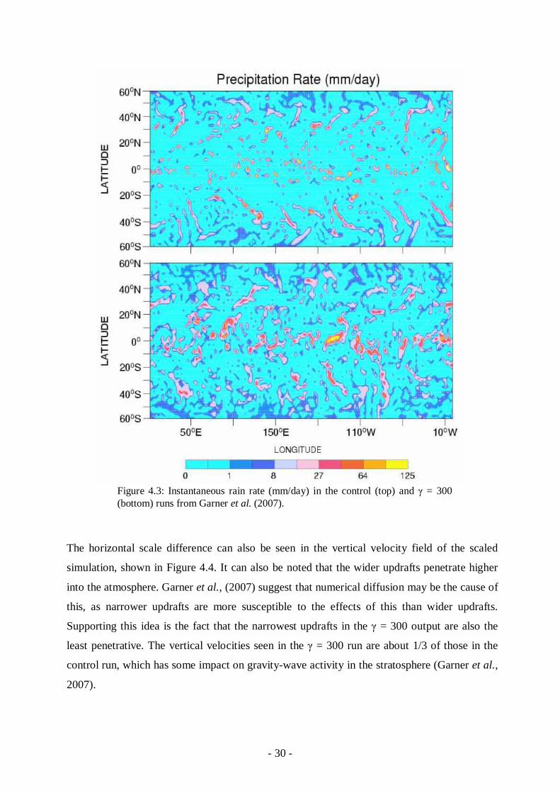
of the convection remained remarkably similar. Figure 4.3 shows the instantaneous rain rate at

equilibrium for the unscaled control and γ = 300 runs from their experiment. Individual storms

in the tropics have a larger horizontal scale, generally between 2 and 8 times the size of those

in the control. Extra-tropical convective structures are also expanded a little. The precipitation

rate remains almost the same, even with the rescaling factor of 300 (Garner et al., 2007).

- 29 -

Figure 4.1: Domain-averaged RCE profiles of Temperature, Cloud fraction and Relative Humidity for the control (solid line) and DARE scaled (dashed line) model runs performed by Kuang et al. (2005).

Figure 4.2: Hourly averaged responses of the domain averaged OLR (top) and precipitation (bottom) to an imposed periodic large-scale forcing in an experiment carried out by Kuang et al. (2005). Control simulations represented by thick lines and DARE by thin. All variables including time are scaled back for the DARE results.

- 30 -

The horizontal scale difference can also be seen in the vertical velocity field of the scaled

simulation, shown in Figure 4.4. It can also be noted that the wider updrafts penetrate higher

into the atmosphere. Garner et al., (2007) suggest that numerical diffusion may be the cause of

this, as narrower updrafts are more susceptible to the effects of this than wider updrafts.

Supporting this idea is the fact that the narrowest updrafts in the γ = 300 output are also the

least penetrative. The vertical velocities seen in the γ = 300 run are about 1/3 of those in the

control run, which has some impact on gravity-wave activity in the stratosphere (Garner et al.,

2007).

Figure 4.3: Instantaneous rain rate (mm/day) in the control (top) and γ = 300 (bottom) runs from Garner et al. (2007).

- 31 -

The DARE rescaling implies that

)1,(),( 1 xwxw ∆≈∆ −γγγ (22)

where w(∆x,γ) is the vertical velocity for a simulation with resolution ∆x and a rescaling factor

of γ. This assumes that the convective updraft buoyancy is independent of γ (Pauluis et al.,

2006). However, experiments find that the vertical velocity is not as sensitive as this (Pauluis

et al., 2006; Garner et al., 2007). Figure 4.5 shows the vertical velocity probability distribution

of a set of simulations carried out by Pauluis et al. (2006) where the resolution is decreased

with the hypohydrostatic rescaling factor chosen such as to keep the effective resolution

constant (ie if the grid size is doubled, the rescaling factor is also doubled). It is clear to see

that the vertical velocities in these simulations, while greatly reduced for large values of γ (at

large resolutions), do not scale as predicted by equation 22. A possible explanation for this is

that the convective updraft buoyancy increases to compensate for the effects of the

hypohydrostatic rescaling (Pauluis et al., 2006).

Figure 4.4: Instantaneous vertical velocity cross section at the Equator at the same time as Figure 4.3. Control run (top) and γ = 300 run (bottom) from Garner et al. (2007). The vertical axis should read km, not m3.

- 32 -

Figure 4.5: Vertical velocity probability distribution function for hypohydrostatically scaled runs with varying resolutions. From Pauluis et al. (2006).

Figure 4.6: Temperature and specific humidity biases in simulations carried out by Pauluis et al. (2006). Bias is difference between named run and the control simulation (∆x=2km, γ = 1 – note that γ is referred to as α in these plots). For each pair of plots the hypohydrostatically rescaled runs are on the left and the coarse resolution runs are on the right.

- 33 -

An important issue in assessing the usefulness of hypohydrostatic simulations is to examine

whether they are better or worse than simulations that simply have a coarser resolution, but

requiring the same computation resources as the scaled runs. Pauluis et al. (2006) compare a

set of hypohydrostatic simulations with coarse resolution runs which have the same resolution.

Figure 4.6 shows the temperature and specific humidity biases between the control run (which

has ∆x=2km, γ = 1) and the two sets of experiments. Both sets of runs show similar

characteristics – a warm bias in the deep troposphere and a dry bias above the boundary layer.

While the temperature bias is significantly smaller in the hypohydrostatic runs, the humidity

bias is greater than in the coarse resolution runs requiring the same respective computational

cost. The humidity bias in the coarse resolution runs is believed to be caused by the inability of

coarse resolutions to simulate shallow overturning and the mixing of low cloud with the

environment (Pauluis and Garner, 2006; Pauluis et al., 2006). While this is not a direct

problem in the hypohydrostatic case, as the rescaling “corrects” for the coarse resolution, the

scaling of the convective overturning time has the effect of reducing the low-level mixing

(Pauluis et al., 2006), leading to a larger dry bias overall.

In terms of predicting cloud water, both sets of simulations produce an excess at low levels,

again caused by the lack of mixing and shallow overturning. This effect is particularly strong if

the vertical wind shear is strong, in which case the coarse resolution runs dramatically

outperform the hypohydrostatic runs. Both sets of runs perform better when predicting cloud

ice, although runs with a high value for γ fail to predict the peak distributions of the ice

correctly (Pauluis et al., 2006).

4.3.2 Impacts on Large Scales

The intention of hypohydrostatic rescaling is that it should not affect the large-scale

circulation, or at least affect it very little. Figure 4.7 shows the zonal-mean differences

between an unscaled control run and a run with γ = 300 carried out by Garner et al. (2007).

The main differences include a weakened subtropical jet, evidenced by the negative

perturbation in the zonal wind, and the related weakening in the Hadley cell, as seen in the

meridional streamfunction. These are related to the decreased latent heating in the tropics, as

the strength of the Hadley cell is extremely sensitive to changes in the latent heating

distribution in the tropics (Hou and Lindzen, 1992). The latent heating in the tropics decreases

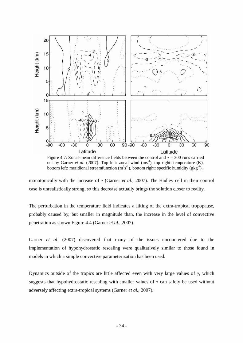
- 34 -

monotonically with the increase of γ (Garner et al., 2007). The Hadley cell in their control

case is unrealistically strong, so this decrease actually brings the solution closer to reality.

The perturbation in the temperature field indicates a lifting of the extra-tropical tropopause,

probably caused by, but smaller in magnitude than, the increase in the level of convective

penetration as shown Figure 4.4 (Garner et al., 2007).

Garner et al. (2007) discovered that many of the issues encountered due to the

implementation of hypohydrostatic rescaling were qualitatively similar to those found in

models in which a simple convective parameterization has been used.

Dynamics outside of the tropics are little affected even with very large values of γ, which

suggests that hypohydrostatic rescaling with smaller values of γ can safely be used without

adversely affecting extra-tropical systems (Garner et al., 2007).

Figure 4.7: Zonal-mean difference fields between the control and γ = 300 runs carried out by Garner et al. (2007). Top left: zonal wind (ms-1), top right: temperature (K), bottom left: meridional streamfunction (m2s-1), bottom right: specific humidity (gkg-1).

- 35 -

A possible issue that has yet to be tested is the effect of the hypohydrostatic rescaling on

intermediate mesoscale systems and their interactions with the large and convective scales

(Pauluis et al., 2006; Garner et al., 2007). However, for modest values of γ (on the order of 2-

8), the approach appears to simulate systems without massively deforming motions on either

the convective or planetary scales, making it a useful tool in global circulation modelling

(Kuang et al., 2005; Peters and Bretherton, 2006, Garner et al., 2007).

- 36 -

5. Model Setup

5.1 The Model

The studies discussed in the previous chapter evaluate the applicability of the hypohydrostatic

rescaling in three dimensional simulations. In order to assess the usefulness of the approach in

two dimensions, a number of simulations in both two and three dimensions were examined.

The model used to carry out the numerical experiments is the Met Office Large Eddy Model.

This is a high resolution model that can be used to represent a variety of atmospheric

situations, from dry turbulence to mesoscale convective systems, over time scales ranging

from hours to days. This model uses a Boussinesq-type system, with parameterizations for

sub-grid-scale turbulence, cloud microphysics and radiation (the radiation scheme was not

used in the experiments).

The basic equation set used in the model is as follows, shown in tensor notation, as in the

documentation associated with the model (Gray et al., 2001):

kjijkj

ji

sij

si

i ux

Bp

xDt

Du Ω−∂∂

+′+

′∂∂−= ε

τρ

δρ

21

(23)

( ) 0=∂∂

isi

ux

ρ (24)

radmphysi

i

s ttx

h

Dt

D

∂∂+

∂∂+

∂∂= θθ

ρθ θ1

(25)

mphys

n

i

qi

s

n

t

q

x

h

Dt

Dq n

∂∂−

∂∂=

ρ1

(26)

In which:

ii x

utDt

D

∂∂+

∂∂= is the Lagrangian rate of change, δij is the Kroneker delta function, εijk is

the alternating pseudo-tensor, u = (u,v,w) is the velocity vector, p' is the pressure perturbation,

ρs is the reference density, B' is the buoyancy, τ is the subgrid stress, Ω is the angular velocity

of the Earth, θ is the potential temperature, hθ is the subgrid scalar flux of θ, mphyst

∂∂θ

is the

- 37 -

source term of θ due to microphysics and radt

∂∂θ

is the source term of θ due to radiation. qn

represents all other scalar variables, with nqh the subgrid scalar flux of qn and mphys

n

t

q

∂∂

the

source term of qn due to microphysics.

The runs have a horizontal grid spacing of 2km, following the reasoning outlined in Section

3.3. The computing time required to run a large simulation limited the domains to 30 grid

points for the 2D runs and a 20x20 square of grid points for the 3D runs. The domain size of

the two-dimensional runs is small enough that it inhibits organisation of convective activity,

as discussed in Section 3.3.1. As discussed in Section 2.3, the mode of organisation has an

effect on the equilibrium state which is avoided by using a small domain.

There are 76 vertical levels within the model height of 20km, with grid spacing varying from

50m near the surface to 500m at the upper limit. The top boundary has a damping layer above

16km, which prevents gravity waves reflecting off the top boundary and causing problems in

the main simulation.

Three-phase microphysics parameterization is used, dividing moisture into various categories.

A total of nine moisture variables represent water vapour, cloud water, cloud ice, rain, snow,

graupel, and number concentrations of ice, snow and graupel.

The model is run over a fixed sea surface of temperature θ = 300K, which avoids any

organization of convection by temperature gradients, as explored by Tompkins (2001b). The

Coriolis effect is ignored by setting ƒ = 0, and no geostrophic wind is imposed. This prevents

any organization or clustering of the convection caused by the effects of rotation. To represent

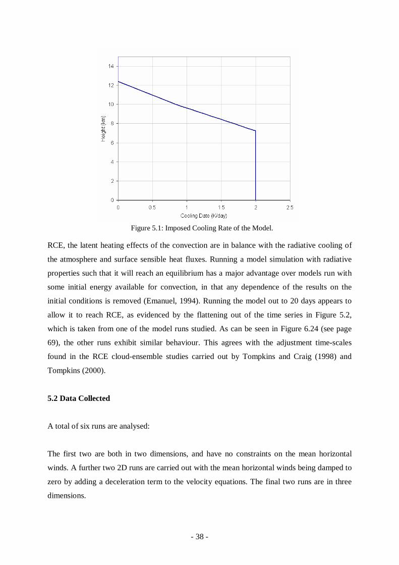
the radiation, instead of using a radiation parameterization, a cooling profile is imposed. This

cooling profile has a cooling rate of 2K/day up to 400mb which then tapers linearly with

pressure to zero at 200mb, as shown in Figure 5.1. This cooling rate matches that in

Tompkins (2000), which should allow for some meaningful comparisons to be made with this

study.

In order to properly assess the effects of the differences in each model run, each run should be

run out until it reaches Radiative-Convective Equilibrium (RCE). When a run has achieved

- 38 -

RCE, the latent heating effects of the convection are in balance with the radiative cooling of

the atmosphere and surface sensible heat fluxes. Running a model simulation with radiative

properties such that it will reach an equilibrium has a major advantage over models run with

some initial energy available for convection, in that any dependence of the results on the

initial conditions is removed (Emanuel, 1994). Running the model out to 20 days appears to

allow it to reach RCE, as evidenced by the flattening out of the time series in Figure 5.2,

which is taken from one of the model runs studied. As can be seen in Figure 6.24 (see page

69), the other runs exhibit similar behaviour. This agrees with the adjustment time-scales

found in the RCE cloud-ensemble studies carried out by Tompkins and Craig (1998) and

Tompkins (2000).

5.2 Data Collected

A total of six runs are analysed:

The first two are both in two dimensions, and have no constraints on the mean horizontal

winds. A further two 2D runs are carried out with the mean horizontal winds being damped to

zero by adding a deceleration term to the velocity equations. The final two runs are in three

dimensions.

Figure 5.1: Imposed Cooling Rate of the Model.

- 39 -

For each of these pairs, one control run has no hypohydrostatic rescaling; or in other words, γ

= 1. This will subsequently be referred to as the unscaled run. The other run has a

hypohydrostatic rescaling of γ = 4. This run will be referred to as the scaled run.

A summary of these runs is given in Table 5.1.

Figure 5.2: Total Column Integrated Water Vapour Timeseries for the 2D model run with no constraining of model winds and a hypohydrostatic rescaling factor of 4.

Runs 2D Unconstrained Winds No Rescaling 2D Unconstrained Winds Scaling, γ= 4 2D Constrained Winds No Rescaling 2D Constrained Winds Scaling, γ= 4 3D No Rescaling 3D Scaling, γ= 4 Table 5.1: Summary of the model runs to be analysed

- 40 -

Data is available for each of these runs at days 0, 2, 4, 6, 8, 10, 12, 14, 15, 16, 17, 18, 19 and

20 of the simulation and includes a wide variety of diagnostics. The majority of these

diagnostics are horizontally averaged and given as a vertical profile, or domain averaged and

given as a time series. Complete 2D fields are also available for some quantities in the 2D

runs only. The diagnostics that will be concentrated upon for analysis are the horizontal and

vertical winds, cloud cover, cloud moisture content, temperature and relative humidity.

- 41 -

6. Discussion of Experiments

Using the model data from the six runs described in the previous chapter, several comparisons

were analysed. Firstly, the effect of the rescaling upon the two dimensional model without

any constraining of horizontal winds is studied, and is discussed in section 6.1. Section 6.2

discusses effect of the hypohydrostatic rescaling upon the model runs with two (6.2.1) and

three (6.2.2) dimensions. The differences between the two and three dimensional model runs

are then analysed in section 6.3, considering the runs with (6.3.1) and without (6.3.2) the

hypohydrostatic rescaling. Finally, a discussion of the results found in sections 6.2 and 6.3

can be found in section 6.4.

6.1 Unconstrained Model Winds in Two Dimensions

As discussed in section 3.3.1, one of the problems encountered when modelling in two

dimensions is the creation of erroneous mean horizontal winds. To investigate the effect of

Figure 6.1: Comparison of Horizontal Winds after 20 Days in the Unscaled (Blue) and Scaled (Red) 2D Model Runs

- 42 -

the hypohydrostatic rescaling on this issue, a pair of two dimensional model runs were carried

out with no damping or constraining of horizontal winds other than the damping taking place

on all variables in the top four kilometres of the model. One run had no hypohydrostatic

scaling, the other was hypohydrostatically scaled with a scaling factor γ = 4. As expected,

fictitious mean horizontal wind speeds were observed in both runs. However, as can be seen

in Figure 6.1, there were large differences between the unscaled and scaled runs. The

maximum mean windspeed in the scaled run is more than six times that of the unscaled run.

The magnitudes of the mean winds in the unscaled run are comparable with the similar

simulation carried out by Tompkins (2000).

As can be seen, the vertical profile is also very different. The unscaled run has two peaks - a

negative peak at around 5.5km, and a smaller positive peak at around 9km. The scaled run has

three distinct peaks; positive peaks at around 4 and 15km, and a strong negative peak at

11km. The height of this strong negative peak in pressure terms is roughly 200mb. This is the

point at which the taper-off of the imposed cooling rate reaches zero. There is a possibility

that these two facts are related, although the mechanism by which this relation would take

effect is unknown. It is impossible to confirm or disprove any relation without running further

scaled model runs with different imposed cooling profiles and analysing the horizontal wind

patterns.

In both runs, the strength of these model winds increases with time. Profiles taken every 4

days through each run are shown in Figure 6.2. The different horizontal scales in the unscaled

and scaled plots should be noted. It is evident from these plots that the windspeeds increased

much more rapidly in the scaled run, with the relative differences in the profiles between days

8 and 20 significantly reduced compared to the unscaled run. The maximum windspeed

recorded in the scaled run does not vary substantially after 8 days, whereas in the unscaled

run it continues to increase right to the end of the model run. This indicates the possibility that

some of the differences noted can be explained based on the DARE interpretation of the

hypohydrostatic rescaling, where timescales are reduced by a factor of γ. The 20 day state of

the hypohydrostatic model run would then be comparable to the 80th day of an unscaled

model run. This timescale rescaling results in a much faster ‘spin up’ time of the model winds

in the hypohydrostatic run. This hypothesis could be tested by running a longer simulation of

the unscaled run and comparing the 80-day output with the 20-day output of the scaled run.

- 43 -

Figure 6.2: Mean Horizontal Wind Speed Profiles at 4, 8, 12, 16 and 20 days in the Unscaled (left) and Scaled (right) 2D Model Runs with no damping of horizontal winds.

- 44 -

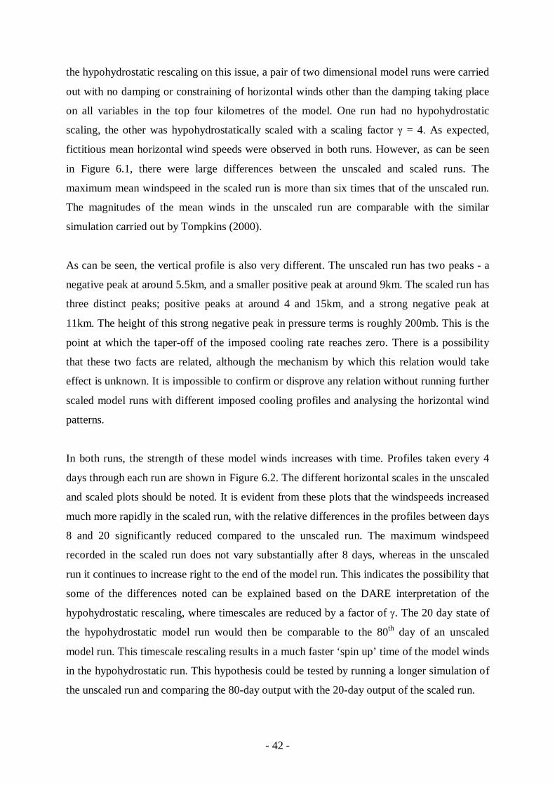
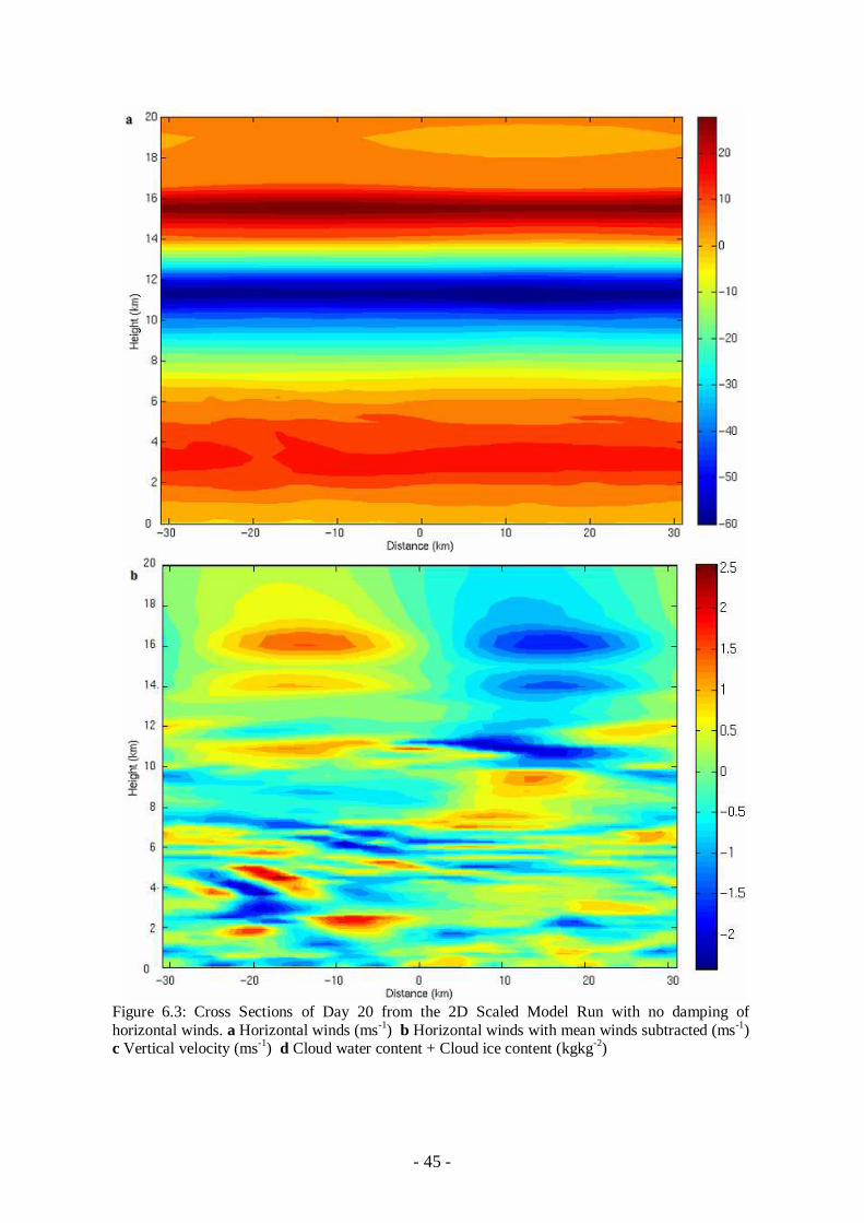
Figure 6.3 shows a variety of 2D ‘snapshots’ from the end of day 20 of the γ = 4 scaled 2D

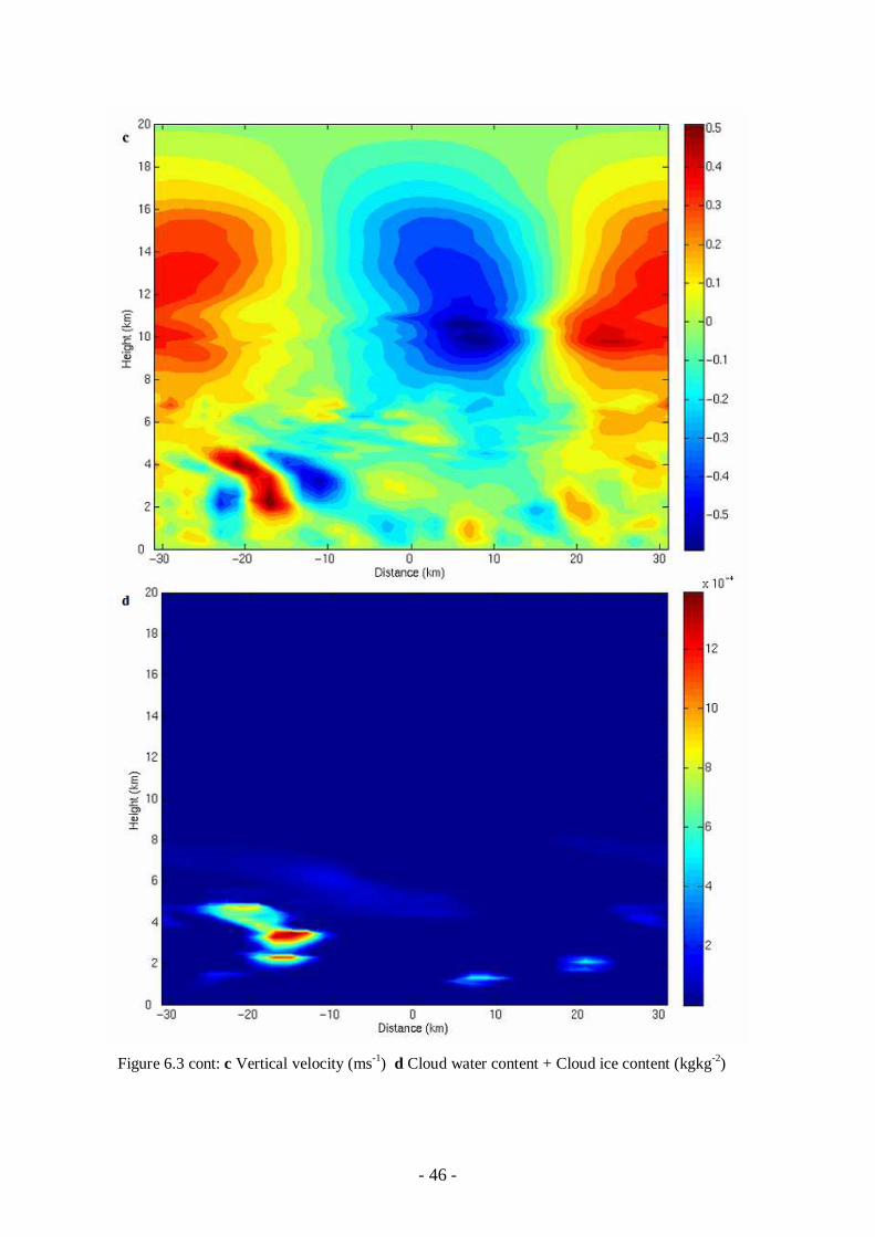
model run with no damping of winds. Figure 6.4 shows the same thing for the unscaled run.

As the model is run in a non-rotating atmosphere, the orientation of the model has no effect.

For the convenience of discussion, it has arbitrarily been chosen to align it East-West, with

East on the right of the cross-sections shown, and West on the left. This convention is carried

throughout this chapter.

As can be seen in Figure 6.3(a), the total wind at any point in the model is dominated by the

horizontal mean wind, masking any smaller patterns. Some structure becomes more apparent

if the mean winds are subtracted from the profile, as in Figure 6.3 (b). This is also true for the

unscaled case, as seen in Figure 6.4. The next step is to analyse this structure with reference to

the vertical motion and cloud moisture content distributions, as shown in Figure 6.3 (c) and

(d) respectively. Cloud moisture content is here calculated by the addition of the cloud water

and cloud ice distributions. This can tell us something about the convective activity in this

simulation and its relationship to the local horizontal winds. In the lower regions of the scaled

domain the wind structures are generally of the order of 10km across (6.4c). In the cloud

moisture cross section (6.3d), a cloud structure can easily be identified at a height of around

4km around 20km West of the centre of the domain. This corresponds to a region of relatively

Easterly moving ascent, with regions of more Westerly moving descent surrounding it. Other

small regions of ascent also have associated regions of cloud moisture and also appear to be

moving relatively Westwards with respect to the mean flow. As the mean winds at this level

are Westerly, it appears that the convective updrafts are opposing this motion, attempting to

rise more vertically in an atmosphere that is attempting to shear them to the East.

Higher in the atmosphere, predominantly above the height of the tropopause, there is a much

larger dry circulation in place, which is moving Westwards with time due to the high mean

winds at that height. This circulation does not appear to be directly connected with the

convective activity lower in the atmosphere. The wavelength of this circulation is equal to the

domain length, and it is impossible to say whether this would remain true for a larger domain

or if multiple patterns would be seen. Partly due to this uncertainty, this feature cannot be

linked conclusively to any feature of the real atmosphere.

- 45 -

Figure 6.3: Cross Sections of Day 20 from the 2D Scaled Model Run with no damping of horizontal winds. a Horizontal winds (ms-1) b Horizontal winds with mean winds subtracted (ms-1) c Vertical velocity (ms-1) d Cloud water content + Cloud ice content (kgkg-2)

- 46 -

Figure 6.3 cont: c Vertical velocity (ms-1) d Cloud water content + Cloud ice content (kgkg-2)

- 47 -

Figure 6.4: As Figure 6.3 but for the Unscaled run.

- 48 -

Figure 6.4 cont.

- 49 -

In the unscaled domain, the large-scale structures in the horizontal and vertical wind fields are

less immediately evident as the fields are generally more disorganised. However, some

similar observation can be made to those in the scaled case – individual cloud systems are

associated with ascent and Westerly flow relative to the overall mean flow. The vertical

motion is slightly less active, resulting in lower concentrations of condensed water in the

atmosphere. The large dry stratospheric circulation seen in the scaled case is also absent here.

Despite the differences in the behaviour of horizontal winds between the two runs, there are

many quantities for which the rescaling has little effect. The temperature profiles, as seen in

Figure 6.5, are very similar, although vertically and time averaged (over days 18-20 of the

runs) temperatures differ by two standard deviations (See Table 6.1 on page 66).

Figure 6.5: Temperature Profiles at 20 days in the Unscaled (blue) and Scaled (green) 2D Model Runs with no damping of horizontal winds.

- 50 -

6.2 Applying the Hypohydrostatic Rescaling

6.2.1 In Two Dimensions

As is customary in 2D simulations (see Section 3.3.1), the problems of the unconstrained

winds discussed in the previous section are circumvented by prescribing a fixed wind profile,

in this case zero at all heights.

This is carried out using an extra relaxation term in the calculation of the horizontal wind at

each timestep, as follows:

τv

termsequationusualt

v −=∂∂

(23)

In this extra term, v is the mean horizontal wind, and τ is an averaging timescale, in this case

chosen to be 10 minutes. This term ‘nudges’ the mean winds back towards zero at each

timestep.

With the mean horizontal winds constrained, negating any differences caused by the larger

mean winds in the hypohydrostatic case, the effects of the hypohydrostatic rescaling on two

dimensional studies can be further studied. The mean winds in these runs are of the order of

1cm/s at their maximum.

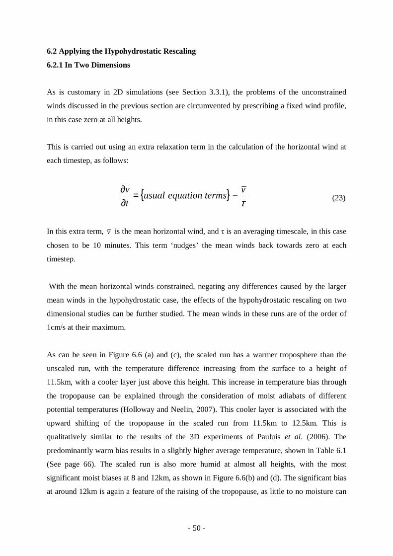
As can be seen in Figure 6.6 (a) and (c), the scaled run has a warmer troposphere than the

unscaled run, with the temperature difference increasing from the surface to a height of

11.5km, with a cooler layer just above this height. This increase in temperature bias through

the tropopause can be explained through the consideration of moist adiabats of different

potential temperatures (Holloway and Neelin, 2007). This cooler layer is associated with the

upward shifting of the tropopause in the scaled run from 11.5km to 12.5km. This is

qualitatively similar to the results of the 3D experiments of Pauluis et al. (2006). The

predominantly warm bias results in a slightly higher average temperature, shown in Table 6.1

(See page 66). The scaled run is also more humid at almost all heights, with the most

significant moist biases at 8 and 12km, as shown in Figure 6.6(b) and (d). The significant bias

at around 12km is again a feature of the raising of the tropopause, as little to no moisture can

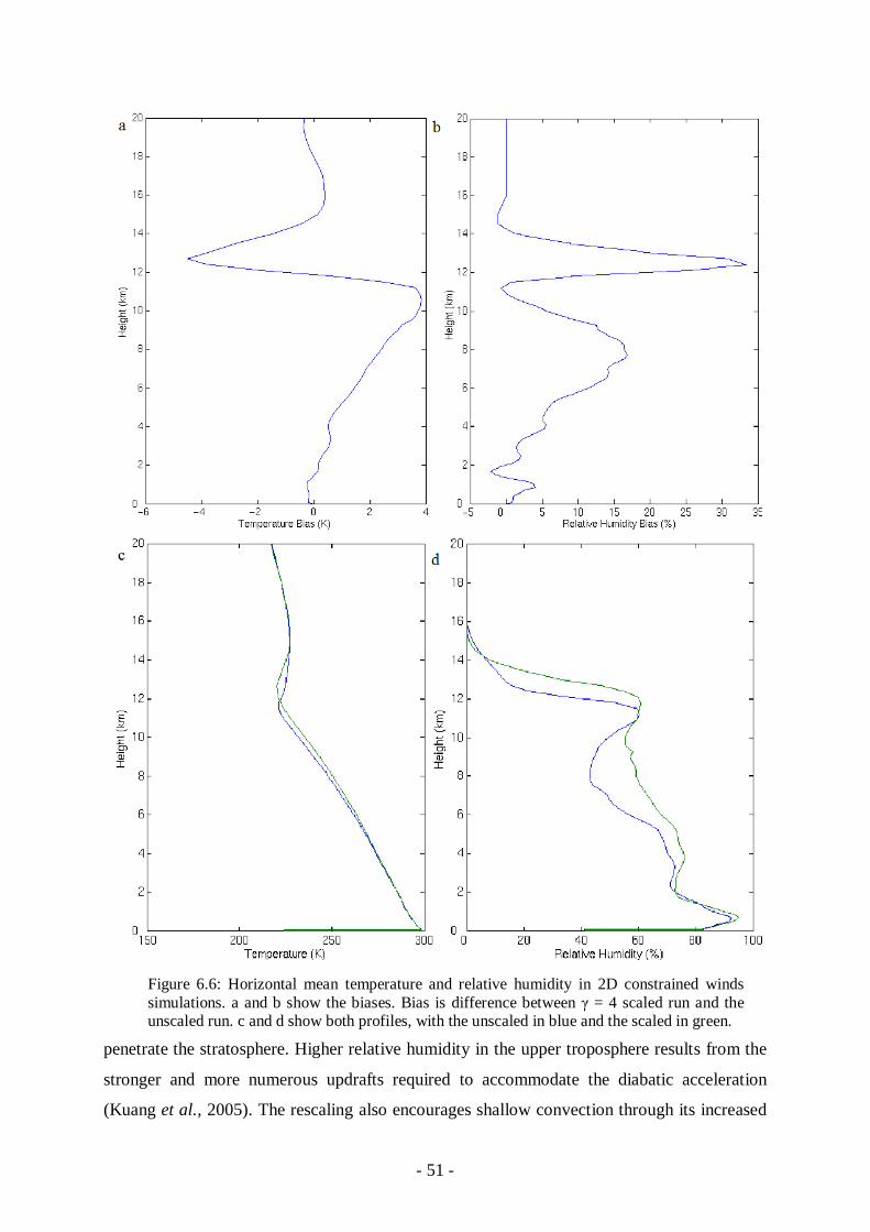
- 51 -

penetrate the stratosphere. Higher relative humidity in the upper troposphere results from the

stronger and more numerous updrafts required to accommodate the diabatic acceleration

(Kuang et al., 2005). The rescaling also encourages shallow convection through its increased

Figure 6.6: Horizontal mean temperature and relative humidity in 2D constrained winds simulations. a and b show the biases. Bias is difference between γ = 4 scaled run and the unscaled run. c and d show both profiles, with the unscaled in blue and the scaled in green.

- 52 -

effective resolution, which increases the moisture content in the lower part of the troposphere

(Garner et al., 2007). The rescaled overturning time, however, prevents shallow overturning,

which reduces the mixing between the boundary layer and the lower troposphere and also

inhibits the dissipation of shallow clouds. This is evidenced in the relative humidity profile by

the slight dry bias at the top of the boundary layer. It can also be seen by viewing the cloud

fraction, shown in Figure 6.7. The high level ice distribution in the hypohydrostatic run is of

similar magnitude but greater height than the unscaled run, which is probably due to the

higher penetration of updrafts in the scaled case, an example of which from day 20 can be

seen in Figure 6.8 (this can also be seen in plots from other days of the model runs). The

deepening of the penetration of the updrafts is assisted by the widening effect the rescaling

has upon them. The entrainment rate of atmospheric air into a cloud has, roughly, an inverse

linear relationship with the width of the updraft, hence wider updrafts have less environmental

air entrained into them per unit area than narrowed updrafts, allowing them to retain more

buoyancy. Updrafts in the scaled run are, on average, around 5km wide, whereas those in the

unscaled simulations average at around 2.5km.

Figure 6.7: Cloud water (left) and cloud ice (right) fractions in the unscaled (blue) and γ = 4 scaled (red) runs, averaged over the final 3 days of the simulations. Cloud water fraction is defined as the fraction of grid points at each level with a cloud water content of more than 0.05g/kg, as in Pauluis et al. (2006), and similarly for cloud ice.

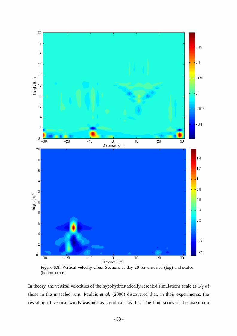
- 53 -

In theory, the vertical velocities of the hypohydrostatically rescaled simulations scale as 1/γ of

those in the unscaled runs. Pauluis et al. (2006) discovered that, in their experiments, the

rescaling of vertical winds was not as significant as this. The time series of the maximum

Figure 6.8: Vertical velocity Cross Sections at day 20 for unscaled (top) and scaled (bottom) runs.

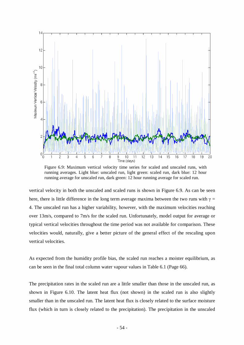
- 54 -

vertical velocity in both the unscaled and scaled runs is shown in Figure 6.9. As can be seen

here, there is little difference in the long term average maxima between the two runs with γ =

4. The unscaled run has a higher variability, however, with the maximum velocities reaching

over 13m/s, compared to 7m/s for the scaled run. Unfortunately, model output for average or

typical vertical velocities throughout the time period was not available for comparison. These

velocities would, naturally, give a better picture of the general effect of the rescaling upon

vertical velocities.

As expected from the humidity profile bias, the scaled run reaches a moister equilibrium, as

can be seen in the final total column water vapour values in Table 6.1 (Page 66).

The precipitation rates in the scaled run are a little smaller than those in the unscaled run, as

shown in Figure 6.10. The latent heat flux (not shown) in the scaled run is also slightly

smaller than in the unscaled run. The latent heat flux is closely related to the surface moisture

flux (which in turn is closely related to the precipitation). The precipitation in the unscaled

Figure 6.9: Maximum vertical velocity time series for scaled and unscaled runs, with running averages. Light blue: unscaled run, light green: scaled run, dark blue: 12 hour running average for unscaled run, dark green: 12 hour running average for scaled run.

- 55 -

run does, however, show a greater degree of variability than that of the scaled run, with peaks

reaching to over 2mm hr-1 compared to less than 1.5mm hr-1 in the scaled run. This agrees

with the general finding that the unscaled 2D runs are more variable than the scaled 2D runs.

Figure 6.10: Time series of precipitation rate in mm hr-1 for the unscaled (top) and γ = 4 scaled (bottom) runs, with raw data in light blue and 12 hour running average in dark blue.

Figure 6.10: Time series of precipitation rate in mm hr-1 for the unscaled (top) and γ = 4 scaled (bottom) runs, with raw data in light blue and 12 hour running average in dark blue.

- 56 -

The deepened convective updrafts of the scaled run exhibit quite strong gravity wave

behaviour especially when they are most penetrative. An example of this can be seen in

Figure 6.11(a-c), taken from day 18 of the γ = 4 run. This activity is not as prominent in the

unscaled run, where the updrafts do not generally penetrate as far, as can also be seen in

Figure 6.11: Day 18 of the 2D constrained-wind simulations. (a) Vertical velocity in the γ = 4 scaled run (ms-1) (b) Horizontal winds in the γ = 4 scaled run (ms-1) (c) Cloud water + ice in the γ = 4 scaled run (kgkg-1) (d) Vertical velocity in the unscaled run (ms-1) (e) Horizontal winds in the unscaled run (ms-1) (f) Cloud water + ice in the unscaled run (kgkg-1)

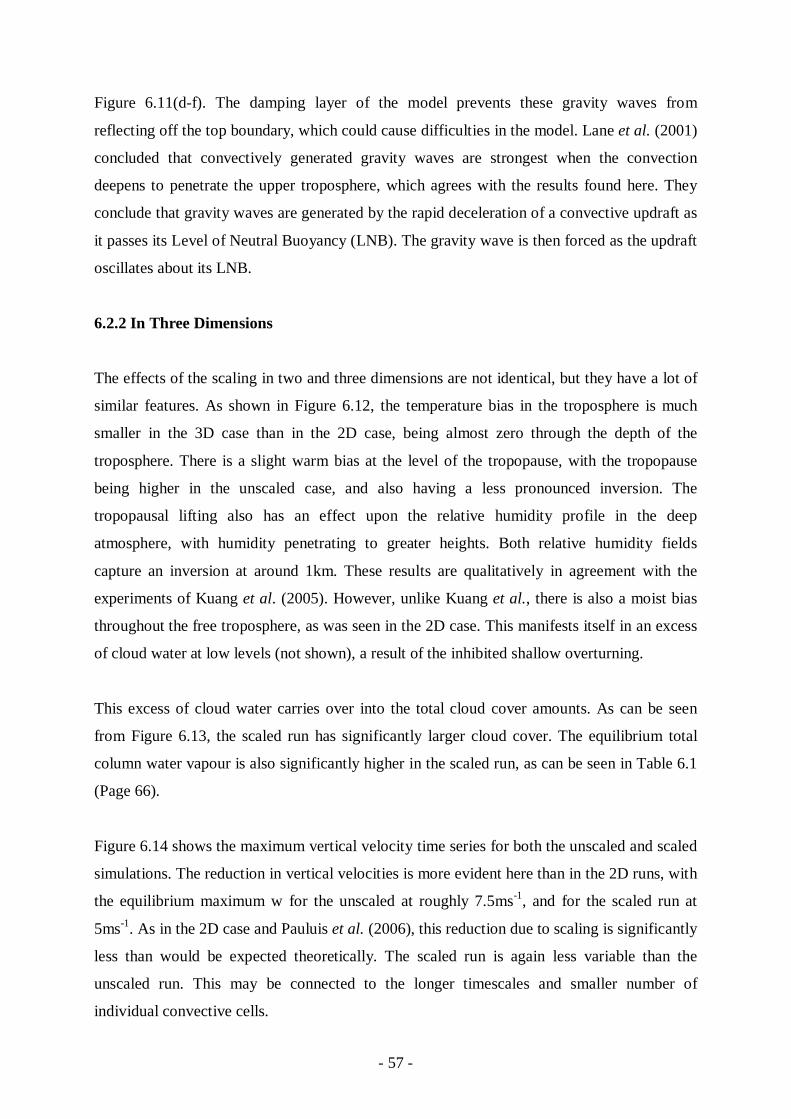
- 57 -

Figure 6.11(d-f). The damping layer of the model prevents these gravity waves from

reflecting off the top boundary, which could cause difficulties in the model. Lane et al. (2001)

concluded that convectively generated gravity waves are strongest when the convection

deepens to penetrate the upper troposphere, which agrees with the results found here. They

conclude that gravity waves are generated by the rapid deceleration of a convective updraft as

it passes its Level of Neutral Buoyancy (LNB). The gravity wave is then forced as the updraft

oscillates about its LNB.

6.2.2 In Three Dimensions

The effects of the scaling in two and three dimensions are not identical, but they have a lot of

similar features. As shown in Figure 6.12, the temperature bias in the troposphere is much

smaller in the 3D case than in the 2D case, being almost zero through the depth of the

troposphere. There is a slight warm bias at the level of the tropopause, with the tropopause

being higher in the unscaled case, and also having a less pronounced inversion. The

tropopausal lifting also has an effect upon the relative humidity profile in the deep

atmosphere, with humidity penetrating to greater heights. Both relative humidity fields

capture an inversion at around 1km. These results are qualitatively in agreement with the

experiments of Kuang et al. (2005). However, unlike Kuang et al., there is also a moist bias

throughout the free troposphere, as was seen in the 2D case. This manifests itself in an excess

of cloud water at low levels (not shown), a result of the inhibited shallow overturning.

This excess of cloud water carries over into the total cloud cover amounts. As can be seen

from Figure 6.13, the scaled run has significantly larger cloud cover. The equilibrium total

column water vapour is also significantly higher in the scaled run, as can be seen in Table 6.1

(Page 66).

Figure 6.14 shows the maximum vertical velocity time series for both the unscaled and scaled

simulations. The reduction in vertical velocities is more evident here than in the 2D runs, with

the equilibrium maximum w for the unscaled at roughly 7.5ms-1, and for the scaled run at

5ms-1. As in the 2D case and Pauluis et al. (2006), this reduction due to scaling is significantly

less than would be expected theoretically. The scaled run is again less variable than the

unscaled run. This may be connected to the longer timescales and smaller number of

individual convective cells.

- 58 -

Figure 6.12: Horizontal mean temperature and relative humidity in the 3D simulations. a and b show the biases. Bias is difference between γ = 4 scaled run and the unscaled run. c and d show both profiles, with the unscaled in blue and the scaled in green.

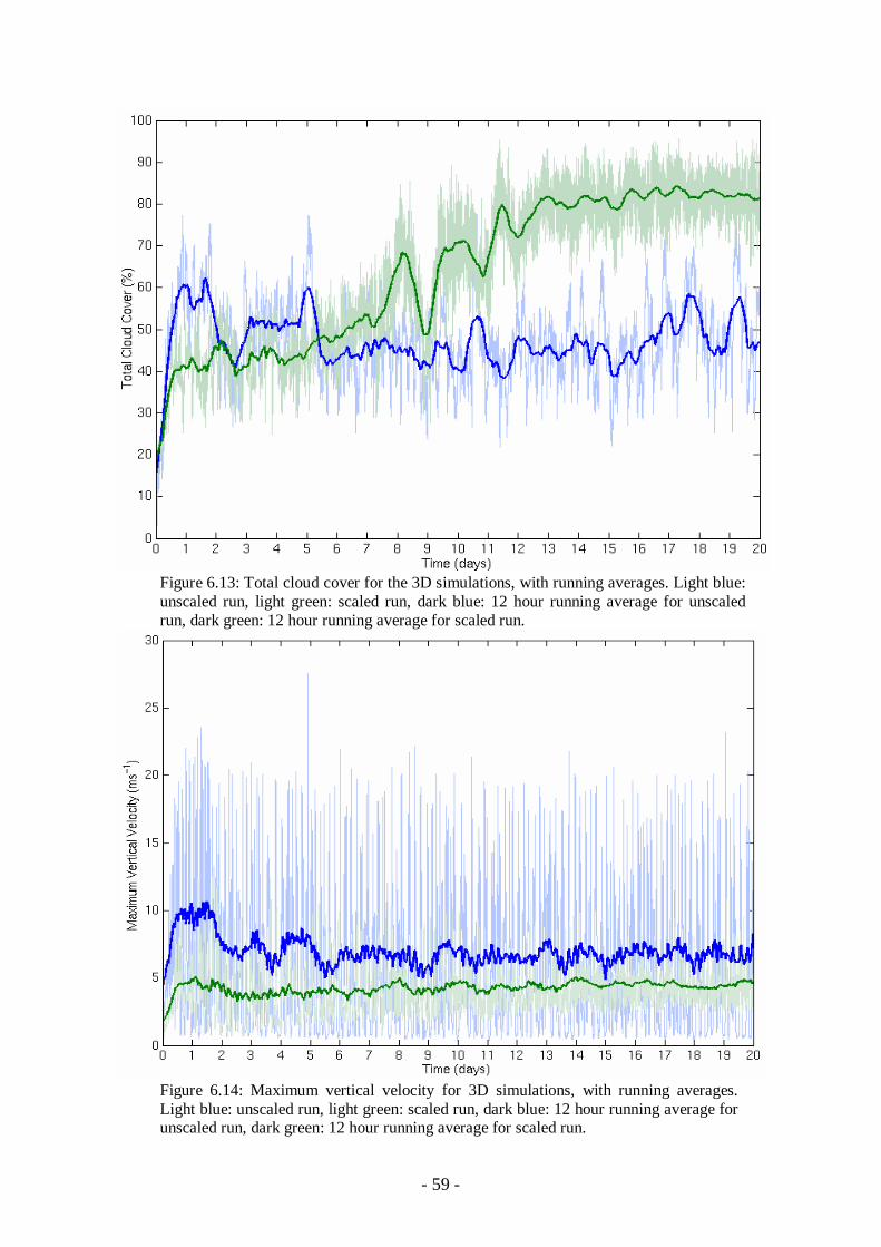
- 59 -

Figure 6.13: Total cloud cover for the 3D simulations, with running averages. Light blue: unscaled run, light green: scaled run, dark blue: 12 hour running average for unscaled run, dark green: 12 hour running average for scaled run.

Figure 6.14: Maximum vertical velocity for 3D simulations, with running averages. Light blue: unscaled run, light green: scaled run, dark blue: 12 hour running average for unscaled run, dark green: 12 hour running average for scaled run.

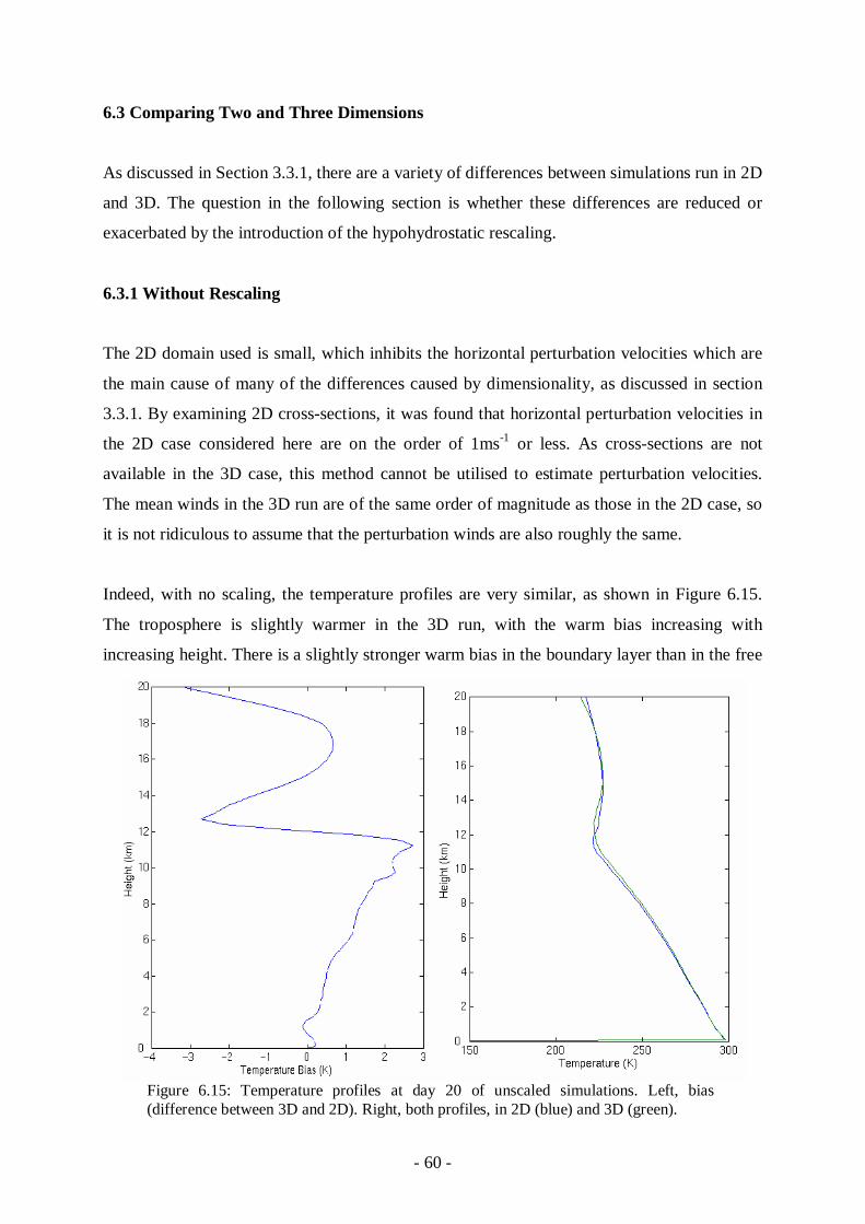
- 60 -

6.3 Comparing Two and Three Dimensions

As discussed in Section 3.3.1, there are a variety of differences between simulations run in 2D

and 3D. The question in the following section is whether these differences are reduced or

exacerbated by the introduction of the hypohydrostatic rescaling.

6.3.1 Without Rescaling

The 2D domain used is small, which inhibits the horizontal perturbation velocities which are

the main cause of many of the differences caused by dimensionality, as discussed in section

3.3.1. By examining 2D cross-sections, it was found that horizontal perturbation velocities in

the 2D case considered here are on the order of 1ms-1 or less. As cross-sections are not

available in the 3D case, this method cannot be utilised to estimate perturbation velocities.

The mean winds in the 3D run are of the same order of magnitude as those in the 2D case, so

it is not ridiculous to assume that the perturbation winds are also roughly the same.

Indeed, with no scaling, the temperature profiles are very similar, as shown in Figure 6.15.

The troposphere is slightly warmer in the 3D run, with the warm bias increasing with

increasing height. There is a slightly stronger warm bias in the boundary layer than in the free

Figure 6.15: Temperature profiles at day 20 of unscaled simulations. Left, bias (difference between 3D and 2D). Right, both profiles, in 2D (blue) and 3D (green).

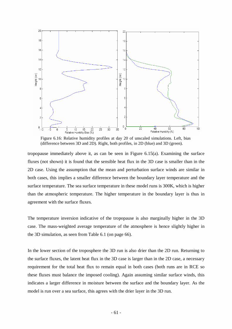
- 61 -

tropopause immediately above it, as can be seen in Figure 6.15(a). Examining the surface

fluxes (not shown) it is found that the sensible heat flux in the 3D case is smaller than in the

2D case. Using the assumption that the mean and perturbation surface winds are similar in

both cases, this implies a smaller difference between the boundary layer temperature and the

surface temperature. The sea surface temperature in these model runs is 300K, which is higher

than the atmospheric temperature. The higher temperature in the boundary layer is thus in

agreement with the surface fluxes.

The temperature inversion indicative of the tropopause is also marginally higher in the 3D

case. The mass-weighted average temperature of the atmosphere is hence slightly higher in

the 3D simulation, as seen from Table 6.1 (on page 66).

In the lower section of the troposphere the 3D run is also drier than the 2D run. Returning to

the surface fluxes, the latent heat flux in the 3D case is larger than in the 2D case, a necessary

requirement for the total heat flux to remain equal in both cases (both runs are in RCE so

these fluxes must balance the imposed cooling). Again assuming similar surface winds, this

indicates a larger difference in moisture between the surface and the boundary layer. As the

model is run over a sea surface, this agrees with the drier layer in the 3D run.

Figure 6.16: Relative humidity profiles at day 20 of unscaled simulations. Left, bias (difference between 3D and 2D). Right, both profiles, in 2D (blue) and 3D (green).

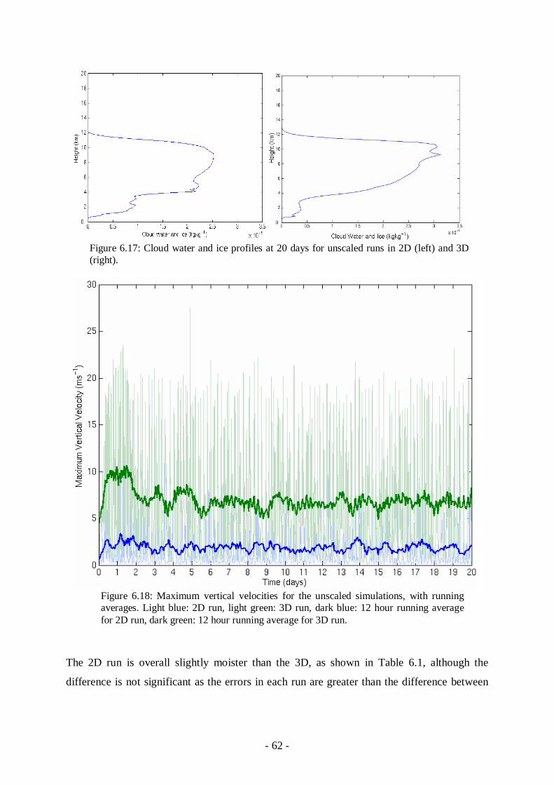
- 62 -

The 2D run is overall slightly moister than the 3D, as shown in Table 6.1, although the

difference is not significant as the errors in each run are greater than the difference between

Figure 6.17: Cloud water and ice profiles at 20 days for unscaled runs in 2D (left) and 3D (right).

Figure 6.18: Maximum vertical velocities for the unscaled simulations, with running averages. Light blue: 2D run, light green: 3D run, dark blue: 12 hour running average for 2D run, dark green: 12 hour running average for 3D run.

- 63 -

them. This is supported by Figure 6.24 (page 69), where it can be seen that the unscaled runs

are very similar as they reach equilibrium.

The relative humidity biases are backed up by the cloud moisture profiles, shown in Figure

6.17. The 2D simulation has a higher cloud water content below 4km, but the 3D simulation

has a higher cloud ice content higher in the troposphere. The total cloud cover in each run

averages out to be roughly equal.

As can be seen in Figure 6.18, the maximum vertical velocities in the 3D case are, on average,

around 7.5ms-1, significantly higher than the 2.5ms-1 of the 2D case, which is in qualitative

agreement with the simulations carried out by Tao et al. (1987). The warmer environment in

the lower tropopause of the 3D run is likely to further increase the updraft intensity, hence

also increasing the differences between 2D and 3D runs.

6.3.2 With Rescaling

In the scaled case, the temperature differences through most of the troposphere are again very

small. The weakness of the temperature inversion in the 3D scaled simulation results in a

warm bias of around 7K at the tropopause, as can be seen in Figure 6.19. The 3D simulation

Figure 6.19: Temperature (left) and Relative Humidity (right) profiles for day 20 of the γ = 4 scaled runs in 2D (blue) and 3D (green).

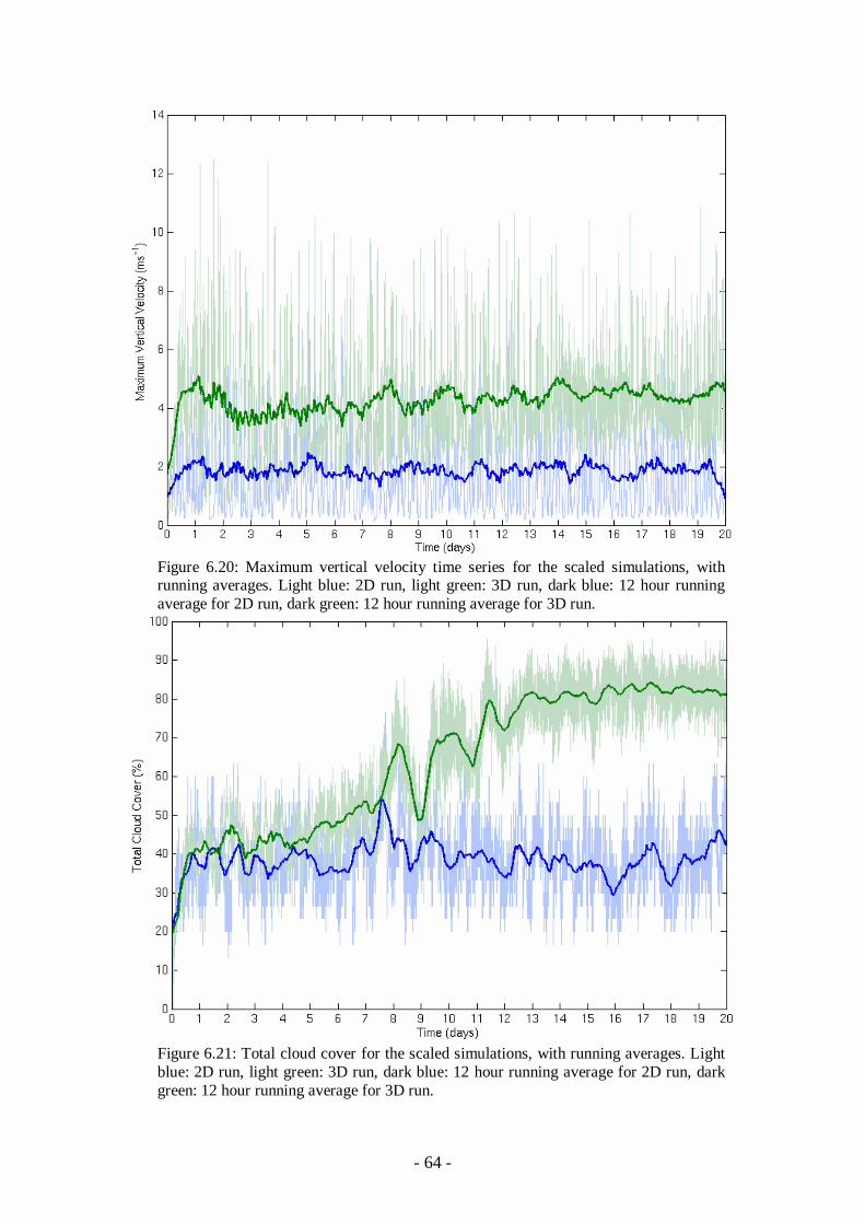
- 64 -

Figure 6.20: Maximum vertical velocity time series for the scaled simulations, with running averages. Light blue: 2D run, light green: 3D run, dark blue: 12 hour running average for 2D run, dark green: 12 hour running average for 3D run.

Figure 6.21: Total cloud cover for the scaled simulations, with running averages. Light blue: 2D run, light green: 3D run, dark blue: 12 hour running average for 2D run, dark green: 12 hour running average for 3D run.

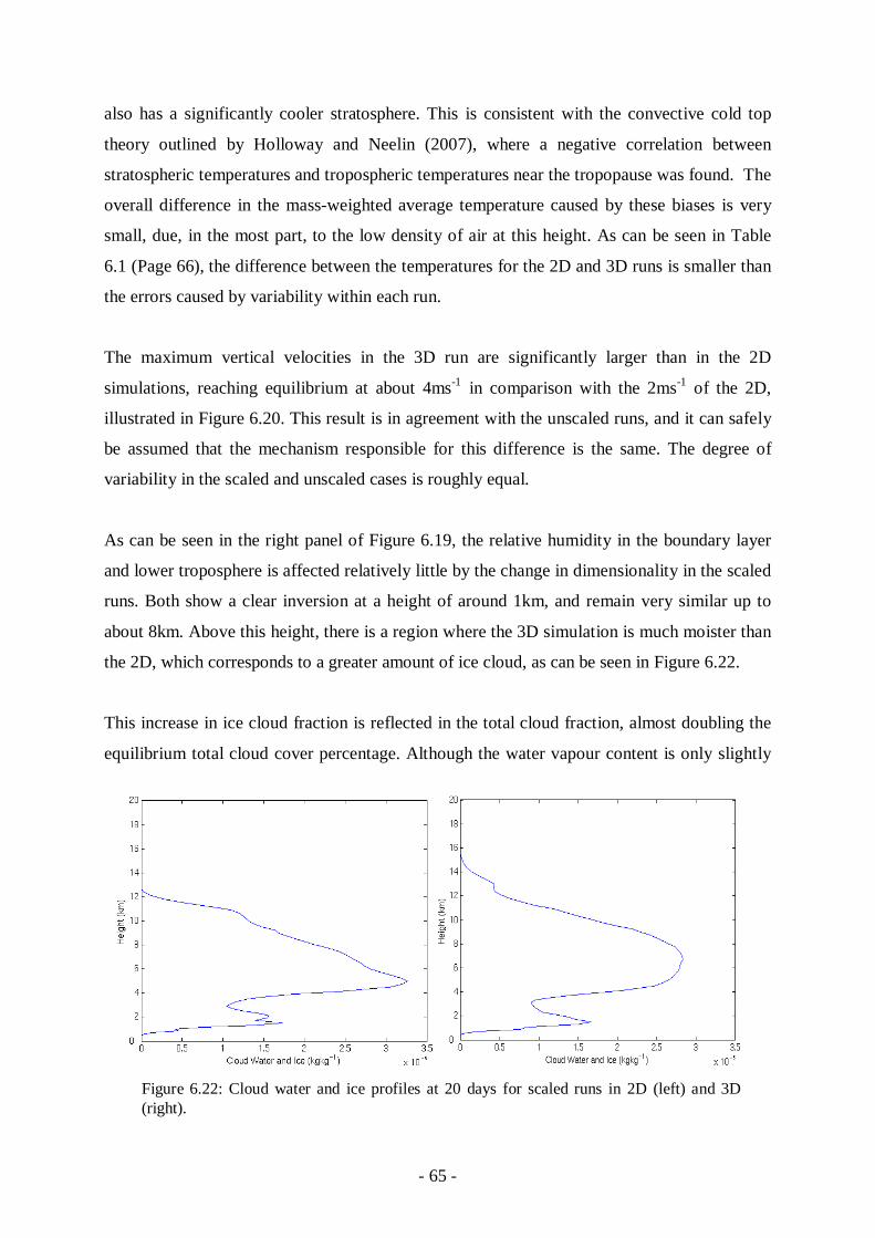
- 65 -

also has a significantly cooler stratosphere. This is consistent with the convective cold top

theory outlined by Holloway and Neelin (2007), where a negative correlation between

stratospheric temperatures and tropospheric temperatures near the tropopause was found. The

overall difference in the mass-weighted average temperature caused by these biases is very

small, due, in the most part, to the low density of air at this height. As can be seen in Table

6.1 (Page 66), the difference between the temperatures for the 2D and 3D runs is smaller than

the errors caused by variability within each run.

The maximum vertical velocities in the 3D run are significantly larger than in the 2D

simulations, reaching equilibrium at about 4ms-1 in comparison with the 2ms-1 of the 2D,

illustrated in Figure 6.20. This result is in agreement with the unscaled runs, and it can safely

be assumed that the mechanism responsible for this difference is the same. The degree of

variability in the scaled and unscaled cases is roughly equal.

As can be seen in the right panel of Figure 6.19, the relative humidity in the boundary layer

and lower troposphere is affected relatively little by the change in dimensionality in the scaled

runs. Both show a clear inversion at a height of around 1km, and remain very similar up to

about 8km. Above this height, there is a region where the 3D simulation is much moister than

the 2D, which corresponds to a greater amount of ice cloud, as can be seen in Figure 6.22.

This increase in ice cloud fraction is reflected in the total cloud fraction, almost doubling the

equilibrium total cloud cover percentage. Although the water vapour content is only slightly

Figure 6.22: Cloud water and ice profiles at 20 days for scaled runs in 2D (left) and 3D (right).

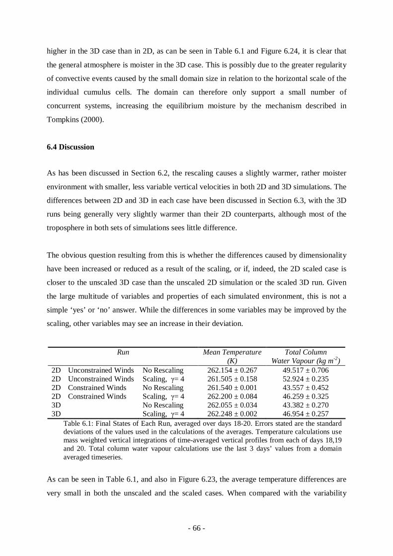
- 66 -

higher in the 3D case than in 2D, as can be seen in Table 6.1 and Figure 6.24, it is clear that

the general atmosphere is moister in the 3D case. This is possibly due to the greater regularity

of convective events caused by the small domain size in relation to the horizontal scale of the

individual cumulus cells. The domain can therefore only support a small number of

concurrent systems, increasing the equilibrium moisture by the mechanism described in

Tompkins (2000).

6.4 Discussion

As has been discussed in Section 6.2, the rescaling causes a slightly warmer, rather moister

environment with smaller, less variable vertical velocities in both 2D and 3D simulations. The

differences between 2D and 3D in each case have been discussed in Section 6.3, with the 3D

runs being generally very slightly warmer than their 2D counterparts, although most of the

troposphere in both sets of simulations sees little difference.

The obvious question resulting from this is whether the differences caused by dimensionality

have been increased or reduced as a result of the scaling, or if, indeed, the 2D scaled case is

closer to the unscaled 3D case than the unscaled 2D simulation or the scaled 3D run. Given

the large multitude of variables and properties of each simulated environment, this is not a

simple ‘yes’ or ‘no’ answer. While the differences in some variables may be improved by the

scaling, other variables may see an increase in their deviation.

As can be seen in Table 6.1, and also in Figure 6.23, the average temperature differences are

very small in both the unscaled and the scaled cases. When compared with the variability

Run Mean Temperature (K)

Total Column Water Vapour (kg m-2)

2D Unconstrained Winds No Rescaling 262.154 ± 0.267 49.517 ± 0.706 2D Unconstrained Winds Scaling, γ= 4 261.505 ± 0.158 52.924 ± 0.235 2D Constrained Winds No Rescaling 261.540 ± 0.001 43.557 ± 0.452 2D Constrained Winds Scaling, γ= 4 262.200 ± 0.084 46.259 ± 0.325 3D No Rescaling 262.055 ± 0.034 43.382 ± 0.270 3D Scaling, γ= 4 262.248 ± 0.002 46.954 ± 0.257

Table 6.1: Final States of Each Run, averaged over days 18-20. Errors stated are the standard deviations of the values used in the calculations of the averages. Temperature calculations use mass weighted vertical integrations of time-averaged vertical profiles from each of days 18,19 and 20. Total column water vapour calculations use the last 3 days’ values from a domain averaged timeseries.

- 67 -

within each individual simulation, however, it can be seen that the anomaly in the scaled case

is decidedly less significant. This is easily seen in Figure 6.23, where the 3D scaled run falls

within the error bar for the 2D scaled run. If the 3D unscaled run is considered as the ‘ideal’

simulation, then it can also be seen that, in terms of average temperature, the 2D scaled run is

in fact the closest other run. This average temperature does, however, mask many differences

which may occur within the data, as a positive bias in one part of the atmosphere can cancel

Figure 6.23: Data from Table 6.1 in graphical format for easier interpretation.

- 68 -

out a negative bias in another part. To investigate this, average temperatures are worked out

for the main four runs, splitting the atmosphere into three layers: the Boundary Layer (0-

1km), the Free Troposphere (1-10km) and the Stratosphere (10-20km). The results are shown

in Table 6.2.

From these values it can be seen that, below the tropopause, the rescaling does decrease the

temperature difference between the 2D and 3D runs, while in the stratosphere the scaled runs

are significantly different. These values have little effect on the overall mean temperature as

the vertical integration is mass weighted.

The picture when it comes to the total column water vapour is rather different. Here, the

anomalies between 2D and 3D are fairly insignificant compared to the variability in both

cases, as seen in Figure 6.23. The unscaled runs here have a very slightly smaller relative

difference, with their difference being 0.8% in comparison with 1.5% for the scaled runs.

Considering this in terms of Figure 6.24, it is not clear which pair of simulations are actually

closer, as it is clear from the figure that the precise difference calculated is highly dependent

on the averaging period chosen. It is very clear, however, that the closest simulation to the

‘ideal’ 3D unscaled run is the unscaled 2D run, as the scaled runs are rather moister.

In both cases, the maximum vertical velocities are higher in the 3D case (see Figures 6.18 and

6.20). The difference between the runs is slightly smaller in the scaled case, which is rather to

be expected as the vertical velocities themselves are smaller due to the rescaling. The

dimensionality difference does not scale linearly with the scaling factor as predicted by the

theory, but is rather less sensitive than this.

Run Mean Boundary Layer Temp. (K)

Mean Free Tropopause Temp.(K)

Mean Stratosphere

Temp. (K) 2D Constrained Winds No Rescaling 294.548 ± 0.059 268.258 ± 0.007 224.919 ± 0.057 2D Constrained Winds Scaling, γ= 4 294.834 ± 0.091 268.694 ± 0.158 223.352 ± 0.194 3D No Rescaling 294.740 ± 0.003 269.005 ± 0.026 224.929 ± 0.077 3D Scaling, γ= 4 294.726 ± 0.001 269.245 ± 0.036 225.095 ± 0.096 Table 6.2: Mean Temperatures, calculated as in the figures in Table 6.1, split into three layers: The Boundary Layer from ground level to 1km, the Free Troposphere from 1km to 10km, and the Stratosphere from 10km to the model top at 20km.

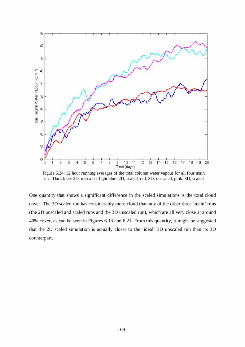
- 69 -

One quantity that shows a significant difference in the scaled simulations is the total cloud

cover. The 3D scaled run has considerably more cloud than any of the other three ‘main’ runs

(the 2D unscaled and scaled runs and the 3D unscaled run), which are all very close at around

40% cover, as can be seen in Figures 6.13 and 6.21. From this quantity, it might be suggested

that the 2D scaled simulation is actually closer to the ‘ideal’ 3D unscaled run than its 3D

counterpart.

Figure 6.24: 12 hour running averages of the total column water vapour for all four main runs. Dark blue: 2D, unscaled, light blue: 2D, scaled, red: 3D, unscaled, pink: 3D, scaled

- 70 -

7. Conclusions

The interaction of cumulus convection with the large-scale climate system is a complicated

issue, which is as yet poorly understood. This lack of understanding translates into a difficulty

in providing an accurate representation of these systems in general circulation models. The

main method used, parameterization, has improved greatly in the past decades but it still has a

long way to go. The hypohydrostatic rescaling method introduced by Kuang et al. (2005)

eliminates the need for a parameterization by increasing the scale of convective motions so

they can be explicitly resolved.

Using a cloud resolving model with a grid size of 2km, this project investigated the validity of

this rescaling in two and three dimensions. When run in two dimensions without any

constraints upon the horizontal mean winds, the rescaled simulation generated mean winds an

order of magnitude greater than those in the unscaled control simulation. A large dry

stratospheric circulation was also produced for which no physical analogue is apparent.

Constraining the mean winds to vanish identically eradicated these issues, and the 2D

simulations in this case were much more similar. The rescaling does appear to increase the

horizontal scale of the convective updrafts as intended, which are also slower and penetrate

further into the atmosphere. The rescaled simulations are also invariably moister than their

unscaled equivalent. These differences are, on the whole, consistent with the changes that

have been found previously. They are also consistent with the three-dimensional runs in this

study.

When comparing the differences between 2D and 3D runs in the scaled and unscaled cases, it

was noted that most properties of the system vary less with dimension in the scaled case than

in the unscaled case, although total cloud cover is a significant exception to this rule. This

property is, indeed, closer to the control runs in the 2D simulation than in the 3D.

Overall, it has been discovered that the known issues in modelling in 2D and the known

issues of the hypohydrostatic rescaling do not compound upon one another, and in fact appear

to have the opposite effect in many properties of the atmosphere, reducing the overall

deviations from “reality”.

- 71 -

This suggests that the use of the rescaling is as valid, and perhaps even better, in two

dimensions as in three. This has implications for approaches that make use of two-

dimensional modelling, such as superparameterization, indicating that these two methods

could possibly be combined.

Further work to evaluate whether this result holds for longer and larger simulations is

required. The domain used in the 2D simulation of this study is small, which inhibits the

organisation of convection and hence has a large effect on the equilibrium state reached. The

differences caused by dimensionality are larger in bigger domains, and while the theory

would suggest that many differences would still be reduced in this case, experimental work is

needed to confirm this.

- 72 -

References

Arakawa, A. (2004). The Cumulus Parameterization Problem: Past, Present, and Future. Journal of. Climate, 17, 2493-2525 Arakawa, A. and W.H. Schubert (1974). Interaction of a Cumulus Cloud Ensemble with the Large-Scale Environment, Part I. Journal of the Atmospheric Sciences, 31, 674-701 Betts, A.K. (1986). A new convective adjustment scheme, Part 1: observational and theoretical basis. Quarterly Journal of the Royal Meteorological Society, 112, 677-691 Bjerknes, J. (1938). Saturated-adiabatic ascent of air through dry-adiabatically descenting environment. Quarterly Journal of the Royal Meteorological Society, 64, 325-330 Browning, G.L. and H.-O. Kreiss (1986). Scaling and Computation of Smooth atmospheric motions. Tellus, 38A, 295-313 Bryan, G.H., J.C. Wyngaard and J.M. Fritsch (2003). Resolution Requirements for the Simulations of Deep Moist Convection. Monthly Weather Review, 131, 2394-2416 Charney, J.G. and A. Eliassen (1964). On the growth of the hurricane depression. Journal of the Atmospheric Sciences, 21, 68-75 Cohen, B.G. and G.C. Craig (2004). The response time of a convective cloud ensemble to a change in forcing. Quarterly Journal of the Royal Meteorological Society, 130, 933-944 Emanuel, K.A. (1986). An air-sea interaction theory for tropical cyclones, Part 1: Steady-state maintenance. Journal of the Atmospheric Sciences, 42, 1062-1071 Emanuel, K.A. (1991). A Scheme for Representing Cumulus Convection in Large-Scale Models. Journal of the Atmospheric Sciences, 48, 2313-2335 Emanuel, K.A. (1994). Atmospheric Convection. Oxford University Press, New York Emanuel, K.A., J.D. Neelin and C.S. Bretherton (1994). On large-scale circulations in convecting atmospheres. Quarterly Journal of the Royal Meteorological Society, 120, 1111-1143 Frank, W.M. (1983). The Cumulus Parameterization Problem. Monthly Weather Review, 111, 1859-1871 Garner, S.T., D.M.W. Frierson, I.M. Held, O. Pauluis and G.K. Vallis (2007). Resolving Convection in a Global Hypohydrostatic Model. Journal of the Atmospheric Sciences, 64, 2061-2075 Gaynor, J.E. and C.F. Ropelewski (1979). Analysis of the convectively modified GATE boundary layer using in situ and acoustic sounder data. Monthly Weather Review, 107, 985-993

- 73 -

Grabowski, W.W. (2001). Coupling Cloud Processes with the Large-Scale Dynamics Using the Cloud-Resolving Convection Parameterization (CRCP). Journal of the Atmospheric Sciences, 58, 978-996 Grabowski, W.W. and M.W. Moncrieff (2001). Large-scale organization of tropical convection in two-dimensional explicit numerical simulations. Quarterly Journal of the Royal Meteorological Society, 127, 445-468 Grabowski, W.W. and P.K. Smolarkiewicz (1999). CRCP: a Cloud Resolving Convection Parameterization for modelling the tropical convecting atmosphere. Physica D, 133, 171-178 Gray, M.E.B., J. Petch, S.H. Derbyshire, A.R. Brown, A.P. Lock, H.A. Swann and P.R.A. Brown (2001). Version 2.3 of The Met Office Large Eddy Model: Part II. Scientific Documentation. Met Office Held, I.M., R.S. Helmer and V. Ramaswamy (1993). Radiative-Convective Equilibrium with Explicit Two-Dimensional Moist Convection. Journal of the Atmospheric Sciences, 50, 3909-3927 Holloway, C.E. and J.D. Neelin (2007). The Convective Cold Top and Quasi Equilibrium. Journal of the Atmospheric Sciences, 64, 1467-1487 Hou and Lindzen (1992). The Influence of Concentrated Heating on the Hadley Circulation. Journal of the Atmospheric Sciences, 49, 1233–1241 Johnson, R.H. and M.E. Nicholls (1983). A composite analysis of the boundary layer accompanying a tropical squall line. Monthly Weather Review, 111, 308-319 Kuang, Z., P.N. Blossey and C.S. Bretherton (2005). A new approach for 3D cloud-resolving simulations of large-scale atmospheric circulation. Geophysical Research Letters, 32, L02809 Kuo, H.L. (1974). Further Studies of the Parameterization of the Influence of Cumulus Convection on Large-Scale Flow. Journal of the Atmospheric Sciences, 31, 1232-1240 Lane, T.P., M.J. Reeder and T.L. Clark (2001). Numerical Modelling of Gravity Wave Generation by Deep Tropical Convection. Journal of the Atmospheric Sciences, 58, 1249–1274 LeMone, M.A., E.J. Zipser and S.B. Trier (1998). The role of environmental shear and thermodynamic conditions in determining the structure and evolution of mesoscale convective systems during TOGA COARE. Journal of the Atmospheric Sciences, 55, 3493-3518 Lindzen, R.S. (2003). The Interaction of Waves and Convection in the Tropics. Journal of the Atmospheric Sciences, 60, 3009-3020 Lipps, F.B. and R.S. Hemler (1986). Numerical Simulation of Deep Tropical Convection associated with Large-Scale Convergence. Journal of the Atmospheric Sciences, 43, 1796-1816

- 74 -

Manabe, S., J. Smagorinsky and R.F. Strickler (1965). Simulated climatology of a general circulation model with a hydrological cycle. Monthly Weather Review, 93, 769-798 Moeng, C.-H., J.C. McWilliams, R. Rotunno, P.P. Sullivan and J. Weil (2004). Investigating 2D Modeling of Atmospheric Convection in the PBL. Journal of the Atmospheric Sciences, 61, 889-903 Pauluis, O. and S. Garner (2006). Sensitivity of radiative-convective equilibrium simulations to horizontal resolution. Journal of the Atmospheric Sciences, 63, 1910–1923 Pauluis, O., D.M.W. Frierson, S.T. Garner, I.M. Held and G.K. Vallis (2006). The hypohydrostatic rescaling and its impacts on modelling of atmospheric convection. Theoretical and Computational Fluid Dynamics, 20, 485-499 Petch, J.C. (2006). Sensitivity studies of developing convection in a cloud-resolving model. Quarterly Journal of the Royal Meteorological Society, 132, 345–358 Peters, M.E. and C.S. Bretherton (2006). Structure of tropical variability from a vertical mode perspective. Theoretical and Computational Fluid Dynamics, 20, 501-524 Randall, D., S. Krueger, C. Bretherton, J. Curry, P. Duynkerke, M. Moncrieff, B. Ryan, D. Starr, M. Miller, W. Rossow, G. Tselioudis and B. Wielicki (2003a). Confronting Models with Data: The GEWEX Cloud Systems Study. Bulletin of the American Meteorological Society, 84, 455-469 Randall, D., M. Khairoutdinov, A. Arakawa and W. Grabowski (2003b). Breaking The Cloud Parameterization Deadlock. Bulletin of the American Meteorological Society, 84, 1547-1564 Saxen, T.R. and S.A. Rutledge (1998). Surface Fluxes and Boundary Layer Recovery in TOGA COARE: Sensitivity to Convective Organization. Journal of the Atmospheric Sciences, 55, 2763-2781 Shutts, G.J. and T.N. Palmer (2007). Convective Forcing Fluctuations in a Cloud-Resolving Model: Relevance to the Stochastic Parameterization Problem. Journal of Climate, 20, 187-202 Tao, W.-K., J. Simpson and S.-T. Soong (1987). Statistical Properties of a Cloud Ensemble: A Numerical Study. Journal of the Atmospheric Sciences, 44, 3175-3187 Tiedtke, M. (1989). A Comprehensive mass Flux Scheme for Cumulus parameterization in Large-Scale Models. Monthly Weather Review, 117, 1779-1800 Tomita, H., H. Miura, S. Iga, T. Nasuno, and M. Satoh (2005). A global cloud-resolving simulation: Preliminary results from an aqua planet experiment. Geophysical Research Letters, 32, L08805 Tompkins, A.M. (2000). The Impact of Dimensionality of Long-Term Cloud-Resolving Model Simulations. Monthly Weather Review, 128, 1521-1535

- 75 -

Tompkins, A.M. (2001a). Organization of Tropical Convection in Low Vertical Wind Shears: The Role of Water Vapour. Journal of the Atmospheric Sciences, 58, 529-545 Tompkins, A.M. (2001b). Organization of Tropical Convection in Low Vertical Wind Shears: The Role of Cold Pools. Journal of the Atmospheric Sciences, 58, 1650-1672 Tompkins, A.M. and G.C. Craig (1998). Radiative-convective equilibrium in a three-dimensional cloud-ensemble model. Quarterly Journal of the Royal Meteorological Society, 124, 2073-2976

- 76 -

Appendix: Implementation of Hypohydrostatic Rescaling in the Met Office LEM

R. S. Plant

This is a short note detailing the implementation of hypohydrostatic rescaling in the Met Office LEM. It is included here in order to clarify the “scaled” LEM simulations performed and to ensure reproducibility of the results. The scaling is to transform the w equation of motion in the inertial frame from

into

where no Reynolds decomposition has been performed. For the complete picture, this note is intended to be read alongside the LEM documentation, particularly the scientific (Gray et al. 2001a) and programming (Gray et al. 2001b) guides. Following the notation of Gray et al. (2001a), the w equation used in the LEM reads

In the hypohydrostatic case this becomes

Notice that the rescaling factor appears not just in the Lagrangian derivative but also in the stress-tensor gradient and Coriolis terms on the right-hand-side. This is, of course, because those terms originate from the Lagrangian derivative in an inertial frame prior to Reynolds decomposition. In order to understand the implementation of the hypohydrostatic scaling in the LEM code, it is convenient to rewrite Eq. 4 as

- 77 -

We consider the implementation in two parts: first, the factor 1/α2 outside the main brackets on the right hand side of Eq. 5; and second, the scaling factors inside the main brackets. 1. The LEM calculates a source term for w such that Eq. 3 is represented as

It updates with the product of this source term and the timestep in subroutine STEPW. Note, however, that the source term at that stage does not include the contribution from the pressure gradient. Rather w is updated with the pressure gradient contribution to Sw in subroutine PSTEP. We scale both of these updates so that

2. It remains to rescale certain of the controbutions to Sw, specifically the first, fourth and fifth terms in the main bracket of Eq. 5. The first and fourth terms may be computed within various subroutines of the LEM, according to which advection scheme has been chosen and whether the simulation is in two or three dimensions. For the present purposes, it suffices to record than the rescalings are performed in the subroutine UVWSRCE or its equivalent1. The fifth term does not need to be explicitly rescaled here since the Coriolis force is absent entirely for the simulations in a non-rotation system that are performed here.

References

Gray, M.E.B., Petch, J., Derbyshire, S.H., Brown, A.R., Lock, A.P., Swann, H.A. and Brown, P.R.A. 2001a. Version 2.3 of the Met Office Large Eddy Model: Part II. Scientific Documentation. Met Office.

Gray, M.E.B., Brown, A.E., Lock, A.P. and Petch, J. 2001b. Version 2.3 of the Met Office

Large Eddy Model: Part III. Software Documentation. Met Office.

1 See Gray et al. (2001b) for the details of “equivalent”.