department of industrial electrical engineering and

Department of Industrial Electrical Engineering and Automation

Fast Estimation of Symmetrical Components Master’s Thesis by Jonas Johansson 2002-10-15

Acknowledgements This work was carried out for ABB Automation Technology Products AB at the Department of Industrial Electrical Engineering and Automation (IEA), Lund University, Sweden, under supervision of Professor Sture Lindahl and Dr. Olof Samuelsson. I wish to thank those persons for their guidance and support. I also would like to thank Bengt Wahnström at Sydkraft AB who provided the Comtrade-files. Big thanks also to all other persons at IEA who have helped me with various things.

Abstract In a power system there is a significant difference between symmetrical conditions and unsymmetrical conditions. Unsymmetrical conditions may occur during power system faults caused by, e.g. lightning, switching surges, insulating contamination or by unsymmetrical loads. Estimation of symmetrical components is a widely used method in protective relays to detect unsymmetrical conditions in three phase power systems. Directional elements and fault classifiers in line protections may, e.g. use negative sequence components. It is of great importance to detect an unsymmetrical condition as fast as possible. Many estimation methods use one cycle Fourier filtering which means an operating time of more than one cycle. The aim for this project is to detect an unsymmetrical condition in a quarter of a cycle or less. This work proposes a method with a filter algorithm using least squares method and variable window size to estimate the symmetrical components. The aim of this MSc work is not to make a real-time implementation of the filter, but to investigate the feasibility of proposed methods by simulations. Therefore the implementation is made in Matlab where the phase signals are known in advance. Various test signals have been used to verify the filter, both basic signals created in Matlab, signals from a simulated power system in Simulink and real measurements from a network during unsymmetrical conditions. The results from these simulations show that it would be possible to detect and estimate a new state in less than a quarter of a 50 Hz cycle. Some limitations in the filter properties are made: It is assumed that outliers and faults shorter than 5 ms are removed in prior signal processing. The filter has been designed under the assumption that the system frequency is known. Furthermore, it is probably necessary to HP-filter the signal to reduce the influence of DC components. Chapter 1 is an explanation to the notations used in the equations. Chapter 2 gives an introduction to the subject. Chapter 3 is a literature study describing what has previously been done in this field. Chapter 4 gives the basic theory of symmetrical components and other methods used in this work. Chapter 5 deals with the algorithms for the Matlab programming and its implementation. Chapter 6 contains simulation results and analyses of the results. Chapter 7 contains conclusions and aspects that have not been covered in this work and finally suggestions for further work are given.

Contents

1 Notation ...............................................................................................................6

2 Introduction..........................................................................................................7 3 Literature study....................................................................................................9 4 Theory................................................................................................................10

4.1 Basic Relations ..............................................................................................10 4.2 Sequence Components in Rectangular Coordinates ......................................12 4.3 Least Squares Method....................................................................................14 4.4 Distortion detection .......................................................................................19 4.5 Determination of deviation limit ...................................................................19

5 Implementation, Matlab programming..............................................................21

5.1 Flow chart ......................................................................................................22 5.2 Comments to the flow chart...........................................................................23 5.3 Considerations ...............................................................................................23

6 Tests, simulations, analysis, results ...................................................................24

6.1 Simulations with signals created in Matlab ...................................................24 6.1.1 Fundamental sinusoidal waves ..................................................................25 6.1.2 Fundamental sinusoidal waves with symmetrical fault (sag) ....................26 6.1.3 Fundamental sinusoidal waves with symmetrical fault (swell) .................27 6.1.4 Fundamental sinusoidal waves with single phase-to-ground fault ............28 6.1.5 Fundamental sinusoidal waves with double phase-to-ground fault...........29 6.1.6 Fundamental sinusoidal waves with three phase-to-ground fault..............30 6.1.7 Noisy sinusoidal waves with single phase-to-ground fault .......................31 6.1.8 Sinusoidal waves with third harmonic, single phase-to-ground fault........32

6.2 Simulations with signals created in Simulink................................................33

6.2.1 Steady state ................................................................................................34 6.2.2 Single phase-to-ground fault......................................................................35 6.2.3 Phase-to-phase fault...................................................................................36 6.2.4 Double phase-to-ground fault ....................................................................37 6.2.5 Three phase fault........................................................................................38 6.2.6 Three phase-to-ground fault ......................................................................39

6.3 Recordings from a real power system ...........................................................40

6.3.1 Case 1 (voltage) .........................................................................................40 6.3.2 Case 1 (current)..........................................................................................41 6.3.3 Case 2 (voltage) .........................................................................................42

6.3.4 Case 2 (current)..........................................................................................43 6.3.5 Case 3 (voltage) .........................................................................................44 6.3.6 Case 3 (current)..........................................................................................45 6.3.7 Case 4 (voltage) .........................................................................................46 6.3.8 Case 4 (current)..........................................................................................47 6.3.9 Case 5 (voltage) .........................................................................................48 6.3.10 Case 5 (current)..........................................................................................49 6.3.11 Case 6 (voltage) .........................................................................................50 6.3.12 Case 7 (voltage) .........................................................................................51 6.3.13 Case 8 (current)..........................................................................................52

7 Conclusions and Suggestions for Future Work .................................................53 8 References..........................................................................................................55 9 Appendix............................................................................................................56

6

1 Notation

as sample of the a-phase signal

bs sample of the b-phase signal

cs sample of the c-phase signal

1A y-coordinate of positive sequence component

1B x-coordinate of positive sequence component

2A y-coordinate of negative sequence component

2B x-coordinate of negative sequence component

0A y-coordinate of zero sequence component

0B x-coordinate of zero sequence component

1S absolute value of positive sequence component

2S absolute value of negative sequence component

0S absolute value of zero sequence component

1φ argument of positive sequence component

2φ argument of negative sequence component

0φ argument of zero sequence component

as1 a-phase positive sequence component

bs1 b-phase positive sequence component

cs1 c-phase positive sequence component

as2 a-phase negative sequence component

bs2 b-phase negative sequence component

cs2 c-phase negative sequence component

as0 a-phase zero sequence component

bs0 b-phase zero sequence component

cs0 c-phase zero sequence component

0ω nominal angular frequency ω actual angular frequency

M window size

t∆ sample period time

k sample number ei residual between actual sample and predicted sample σ standard deviation of residuals

7

2 Introduction Traditionally, a complete relay protection system consists of different kind of relays: over current relays, earth fault current relays, over voltage relays, differential relays and distance relays. Common for all these are that they use instrument transformers to measure the conditions of the power system. The introduction of microprocessor protective relays in the 1980s offered new possibilities and benefits, such as: flexibility, lower costs, reliability with self-checking capability, and fault location/event-recording capabilities with local and remote reporting. Samples are taken from the protected object that then get processed in a microprocessor. This led to the possibility to use symmetrical components in distance relays. The positive sequence component exists during all system conditions and is dominating during symmetrical conditions, including three phase faults. The negative sequence component exists during unsymmetrical conditions. The zero sequence component exists when ground is involved in a fault. During symmetrical and stationary conditions the symmetrical components have stationary values, the positive-sequence voltage equals the peak phase-to-earth voltage of the a-phase and the negative and zero-sequences are close to zero. When a fault occurs the symmetrical components will change and reach new stationary values that indicate a new state in the power system. To detect fault conditions as fast as possible is of great importance. The faster a fault is detected, the faster actions can be made to disconnect the faulted line. The risk for transient instability is then reduced which in turn increases the transmission capacity. This means that the equipment can be designed in a more efficient way, which in turn can reduce the overall cost for a power system. Figure 2.1 shows the transmission capacity-fault clearing time relation for a symmetrical three-phase fault where the negative and the zero-sequence components are very close to zero, and a single-phase fault. A phase-to-phase-to-earth fault is almost as serious as a three-phase fault.

TRANSMISSION CAPACITY LIMITED BY RISK FOR TRANSIENT INSTABILITY

Fault Clearing T ime

[MW

]

Three-phase Fault and Three-phase Reclosing

Single-phase Fault and Single-phase Reclosing

Figure 2.1. The relationship between fault clearing time and transmission capacity.

8

Another application is to use the negative zero sequence current for generator protection. Here the operating speed is, however, not as important as for line protection. An advantage of the proposed method is that it can be applied at frequencies that deviate from the nominal frequency. With these aspects kept in mind it is clear that fast estimation methods is of great importance. On the market there is a demand for estimation methods faster than 10 ms. The aim of this study is to detect an unsymmetrical condition within a quarter of a 50 Hz cycle, i.e.5 ms. Many fast estimation methods (please refer the literature study) use one cycle Fourier filtering which means a computation time of at least one period. The approach used here uses variable window size and statistical analysis to detect a new state. This study is made using Matlab in order to investigate if it might be possible to implement the method in a real microprocessor protective relay. In Matlab, the sample sequences have to be known in advance and hence it does not work in real time, even though the algorithm treat the samples as they appear in real time. As a consequence of that, the program cannot directly be implemented in a real microprocessor protective relay. Main focus is to investigate whether this new approach seems to work or not in a simulation environment. Both sequences generated in Matlab and Simulink as well as real network measurements from Sydkraft AB have been used to verify the program. In the Matlab program, no considerations have been taken whether the samples represent voltages or currents. The input samples are just referred to as signals. Frequency deviations have not been considered, it is assumed that the frequency is known. The study is limited to the estimation of the symmetrical components. Further steps in the relaying process, such as trip decisions, fault location and fault classification, are not within the scope. The sampling frequency used in the simulations is 1000 Hz. One might ask why not just simply increase the sampling frequency to get faster estimations. The answer is that the 1000 Hz frequency has a long tradition in computer based relay protection systems and has become the standard sampling rate for ABB protection systems. Other manufacturers use sampling rates ranging from 600 to 1440 Hz. Attempts to use sampling rates up to about 4000 Hz have been made.

9

3 Literature study

Much works have been done in this subject before and most of them use Fourier algorithms in different forms that need at least one cycle to estimate the sequence components. Here follows a short description of those who are of interest.

One of the earliest computer implementations was presented by Degens in 1982 [1], see list of references in chapter 8. The paper describes an implementation of a digital filter with constant sampling window. Six samples per period are used. The estimation time is poor though, 33 ms, or two cycles, at 60 Hz. Kolla [2] uses a method called block pulse functions. The fundamental frequency components are first computed with block pulse functions and then transformed into symmetrical components. It is stated that the sequence components can be detected within a cycle. Lobos shows in [3] a comparison between a Fourier algorithm with constant sampling and a Fourier algorithm with variable sampling window and finally a Kalman algorithm. The estimation times are not mentioned, neither is the zero sequence component calculated by the algorithms. Reference [4] uses a technique based on stochastic estimation theory. Bad measurements have effect on the final accuracy of the estimation and the estimation time is about 112 ms. None of these methods have an estimation time less than at least ¾ of a fundamental period time. An exception is reference [5] which claims to estimate the sequence components with only one sample delay. It is only verified with fundamental frequencies without noise and with step changes in the input signals. A three-point median filter is utilized to remove the noise that appears during the transient process. The results are confusing though, since the sequence components have the shape of sinusoidal waves when they are supposed to be constant when the input signals are stationary. A description of how symmetrical components can be used in protection systems is presented in [6].

10

4 Theory The basic idea with this work is to implement a filter that transforms sampled values from the phase signals to symmetrical components. During steady state conditions the order of the filter is twenty that means that the twenty most recent samples are used in the estimation. The least-square method is used to restrain noise and harmonics and to find the parameters defining the symmetrical components. This gives a linear equation system with six equations and six unknown parameters (A1, B1, A2, B2, A0, B0) that can be solved. By predicting the next samples and comparing them with the actual samples it is possible to detect new states. If the next sample exceeds a certain level, a new state is considered to have occurred. If a new state occurs the stored samples will be erased and the window size will be minimized. By doing this the pre-fault samples do not affect the new estimation. The window length is then built up again step-by-step until it reaches its full size. The estimates become more accurate as the size increases. With variable window size it is possible to make faster and better estimations of the symmetrical components compared to the use of a constant window size. 4.1 Basic Relations The theory of symmetrical components was developed by C.L. Fortescue in 1918 [7] and has become a very important tool for the analysis of power systems. Only the definition of symmetrical components is given here, but more information in this topic can be found in [8] for instance. A set of three-phase signals, (voltage or current), can be resolved into the following three sets of sequence components:

1. Zero-sequence components, consisting of three phasors with equal magnitudes and with zero phase displacement.

Figure 4.1 2. Positive-sequence components, consisting of three phasors with equal magnitudes, ±120°

phase displacement, and positive phase sequence.

Figure 4.2.

a

b

c

a

b

c

11

c

3. Negative-sequence components, consisting of three phasors with equal magnitudes, ±120° phase displacement, and negative phase sequence.

Figure 4.3. The phase signals can be expressed in discrete time as:

,.........2,1,0

)sin()(

)sin()(

)sin()(

=

+∆=+∆=+∆=

kfor

tkSks

tkSks

tkSks

ccc

bbb

aaa

ϕωϕωϕω

(4.1)

This means that the signals are defined by the six parameters Sa, Sb, Sc, ϕa, ϕb and ϕc.

These phase signals can be expressed as a sum of the positive-, negative- and zero-sequence components.

)()()()(

)()()()(

)()()()(

021

021

021

ksksksks

ksksksks

ksksksks

cccc

bbbb

aaaa

++=++=++=

(4.2)

The positive-sequence components are defined as follows:

−+∆⋅=

−+∆⋅=

+∆⋅=

3

4sin)(

3

2sin)(

)sin()(

111

111

111

πφω

πφω

φω

tkSks

tkSks

tkSks

c

b

a

(4.3)

a

b

12

The negative-sequence components are defined as follows:

−+∆⋅=

−+∆⋅=

+∆⋅=

3

2sin)(

3

4sin)(

)sin()(

222

222

222

πφω

πφω

φω

tkSks

tkSks

tkSks

c

b

a

(4.4)

The zero-sequence components are defined as follows:

( )( )000

000

000

sin)(

sin)(

)sin()(

φωφωφω

+∆⋅=+∆⋅=+∆⋅=

tkSks

tkSks

tkSks

c

b

a

(4.5)

This means that the original phase signals can be expressed by symmetrical components which are defined by the six parameters S1, S2, S0, φ 1, φ 2 and φ 0. In this way the symmetrical components are represented in polar coordinates. Based on the sampled values of the phase signals we want to find those six parameters. 4.2 Sequence Components in Rectangular Coordinates In order to simplify the parameter estimation it is a good idea to use rectangular coordinates instead of polar coordinates. From now on we assume that the angular frequency is equal to the nominal angular frequency and the variable θk=kω0∆t is used to further simplify the notation. The sequence components then become as follows: The positive-sequence components:

−⋅+

−⋅=

−⋅+

−⋅=

⋅+⋅=

3

4sin

3

4cos)(

3

2sin

3

2cos)(

)sin()cos()(

111

111

111

πθπθ

πθπθ

θθ

kkc

kkb

kka

BAks

BAks

BAks

(4.6)

The relations between S1, φ 1 and the new parameters A1, B1 are as follows:

=

+=

1

11

21

211

arctanB

A

BAS

φ (4.7)

13

The negative-sequence components:

−⋅+

−⋅=

−⋅+

−⋅=

⋅+⋅=

3

2sin

3

2cos)(

3

4sin

3

4cos)(

)sin()cos()(

222

222

222

πθπθ

πθπθ

θθ

kkc

kkb

kka

BAks

BAks

BAks

(4.8)


=

+=

2

22

22

222

arctanB

A

BAS

φ (4.9)

The zero-sequence components:

( ) ( )( ) ( )kkc

kkb

kka

BAks

BAks

BAks

θθθθθθ

sincos)(

sincos)(

)sin()cos()(

000

000

000

⋅+⋅=⋅+⋅=⋅+⋅=

(4.10)


=

+=

0

00

20

200

arctanB

A

BAS

φ (4.11)

Finally, by putting (4.6), (4.8) and (4.10) into (4.2) makes that the original sampled phase signals can be expressed as follows: (4.12)

( ) ( )

( ) ( )kkkkkkc

kkkkkkb

kkkkkka

BABABAks

BABABAks

BABABAks

θθπθπθπθπθ

θθπθπθπθπθ

θθθθθθ

sincos3

2sin

3

2cos

3

4sin

3

4cos)(

sincos3

4sin

3

4cos

3

2sin

3

2cos)(

)sin()cos()sin()cos()sin()cos()(

002211

002211

002211

⋅+⋅+

−⋅+

−⋅+

−⋅+

−⋅=

⋅+⋅+

−⋅+

−⋅+

−⋅+

−⋅=

⋅+⋅+⋅+⋅+⋅+⋅=

14

4.3 Least Squares Method The least squares method is used to estimate unknown parameters for a function based on samples from a distribution, see [10]. In this case the six unknown parameters are: A1, B1, A2, B2, A0 and B0. The function that shall be minimized is then: (4.13)

To find the minimum of the function it is differentiated with respect to each parameter yielding six equations. Each equation is then set equal to zero as follows:

0),,,,,(

0),,,,,(

0),,,,,(

0),,,,,(

0),,,,,(

0),,,,,(

0

002211

0

002211

2

002211

2

002211

1

002211

1

002211

=

=

=

=

=

=

dB

BABABAdV

dA

BABABAdV

dB

BABABAdV

dA

BABABAdV

dB

BABABAdV

dA

BABABAdV

(4.14)

( ) [

] [

( ) ( ) ] [

( ) ( ) ]200221

1

1

0

20022

11

1

0

200

1

0

2211002211

)(sincos3

2sin

3

2cos

3

4sin

3

4cos)(sincos

3

4sin

3

4cos

3

2sin

3

2cos)()sin()cos(

)sin()cos()sin()cos(,,,,,

ksBABAB

AksBABA

BAksBA

BABABABABAV

ckkkkk

k

M

k

bkkkk

kk

M

k

akk

M

k

kkkk

−⋅+⋅+

−⋅+

−⋅+

−⋅+

−⋅+−⋅+⋅+

−⋅+

−⋅

+

−⋅+

−⋅+−⋅+⋅

+⋅+⋅+⋅+⋅=

∑

∑

∑

−

=

−

=

−

=

θθπθπθπθ

πθθθπθπθ

πθπθθθ

θθθθ

15

Applying (4.13) on the function (4.14) gives following six equations: (4.15)

[

] [

( ) ( ) ] [

( ) ( ) ]

−⋅+

−⋅+⋅

=

−⋅⋅+⋅+

−⋅+

−⋅+

−⋅+

−⋅+

−⋅⋅+⋅+

−⋅+

−⋅

+

−⋅+

−⋅+⋅⋅+⋅

+⋅+⋅+⋅+⋅

∑

∑

∑

∑

−

=

−

=

−

=

−

=

3

4cos)(

3

2cos)()cos()(

3

4cossincos

3

2sin

3

2cos

3

4sin

3

4cos

3

2cossincos

3

4sin

3

4cos

3

2sin

3

2cos)cos()sin()cos(

)sin()cos()sin()cos(

1

0

00221

1

1

00022

11

1

000

1

02211

πθπθθ

πθθθπθπθπθ

πθπθθθπθπθ

πθπθθθθ

θθθθ

kckbk

M

ka

kkkkkk

k

M

kkkkkk

kk

M

kkkk

M

kkkkk

ksksks

BABAB

ABABA

BABA

BABA

(4.16)

[

] [

( ) ( ) ] [

( ) ( ) ]

−⋅+

−⋅+⋅

=

−⋅⋅+⋅+

−⋅+

−⋅+

−⋅+

−⋅+

−⋅⋅+⋅+

−⋅+

−⋅

+

−⋅+

−⋅+⋅⋅+⋅

+⋅+⋅+⋅+⋅

∑

∑

∑

∑

−

=

−

=

−

=

−

=

3

4sin)(

3

2sin)()sin()(

3

4sinsincos

3

2sin

3

2cos

3

4sin

3

4cos

3

2sinsincos

3

4sin

3

4cos

3

2sin

3

2cos)sin()sin()cos(


1

0

00221

1

1

00022

11

1

000

1

02211

πθπθθ



πθπθθθθ

θθθθ

kckbk

M

ka

kkkkkk

k

M

kkkkkk

kk

M

kkkk

M

kkkkk

ksksks

BABAB

ABABA

BABA

BABA

(4.17)

[

] [

( ) ( ) ] [

( ) ( ) ]

−⋅+

−⋅+⋅

=

−⋅⋅+⋅+

−⋅+

−⋅+

−⋅+

−⋅+

−⋅⋅+⋅+

−⋅+

−⋅

+

−⋅+

−⋅+⋅⋅+⋅

+⋅+⋅+⋅+⋅

∑

∑

∑

∑

−

=

−

=

−

=

−

=

3

2cos)(

3

4cos)()cos()(

3

2cossincos

3

2sin

3

2cos

3

4sin

3

4cos

3

4cossincos

3

4sin

3

4cos

3

2sin

3

2cos)cos()sin()cos(


1

0

00221

1

1

00022

11

1

000

1

02211

πθπθθ



πθπθθθθ

θθθθ

kckbk

M

ka

kkkkkk

k

M

kkkkkk

kk

M

kkkk

M

kkkkk

ksksks

BABAB

ABABA

BABA

BABA

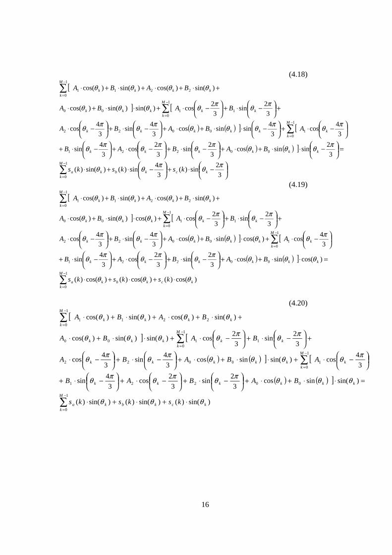
16

(4.18)

[

] [

( ) ( ) ] [

( ) ( ) ]

−⋅+

−⋅+⋅

=

−⋅⋅+⋅+

−⋅+

−⋅+

−⋅+

−⋅+

−⋅⋅+⋅+

−⋅+

−⋅

+

−⋅+

−⋅+⋅⋅+⋅

+⋅+⋅+⋅+⋅

∑

∑

∑

∑

−

=

−

=

−

=

−

=

3

2sin)(

3

4sin)()sin()(

3

2sinsincos

3

2sin

3

2cos

3

4sin

3

4cos

3

4sinsincos

3

4sin

3

4cos

3

2sin

3

2cos)sin()sin()cos(


1

0

00221

1

1

00022

11

1

000

1

02211

πθπθθ



πθπθθθθ

θθθθ

kckbk

M

ka

kkkkkk

k

M

kkkkkk

kk

M

kkkk

M

kkkkk

ksksks

BABAB

ABABA

BABA

BABA

(4.19)

[

] [

( ) ( ) ] [

( ) ( ) ]

)cos()()cos()()cos()(

)cos(sincos3

2sin

3

2cos

3

4sin

3

4cos)cos(sincos

3

4sin

3

4cos

3

2sin

3

2cos)cos()sin()cos(


1

0

00221

1

1

00022

11

1

000

1

02211

kckbk

M

ka

kkkkkk

k

M

kkkkkk

kk

M

kkkk

M

kkkkk

ksksks

BABAB

ABABA

BABA

BABA

θθθ

θθθπθπθπθ

πθθθθπθπθ

πθπθθθθ

θθθθ

⋅+⋅+⋅

=⋅⋅+⋅+

−⋅+

−⋅+

−⋅+

−⋅+⋅⋅+⋅+

−⋅+

−⋅

+

−⋅+

−⋅+⋅⋅+⋅

+⋅+⋅+⋅+⋅

∑

∑

∑

∑

−

=

−

=

−

=

−

=

(4.20)

[

] [

( ) ( ) ] [

( ) ( ) ]

)sin()()sin()()sin()(

)sin(sincos3

2sin

3

2cos

3

4sin

3

4cos)sin(sincos

3

4sin

3

4cos

3

2sin

3

2cos)sin()sin()cos(


1

0

00221

1

1

00022

11

1

000

1

02211

kckbk

M

ka

kkkkkk

k

M

kkkkkk

kk

M

kkkk

M

kkkkk

ksksks

BABAB

ABABA

BABA

BABA

θθθ

θθθπθπθπθ

πθθθθπθπθ

πθπθθθθ

θθθθ

⋅+⋅+⋅

=⋅⋅+⋅+

−⋅+

−⋅+

−⋅+

−⋅+⋅⋅+⋅+

−⋅+

−⋅

+

−⋅+

−⋅+⋅⋅+⋅

+⋅+⋅+⋅+⋅

∑

∑

∑

∑

−

=

−

=

−

=

−

=

17

Now the six equations can be arranged in an equation system and solved to give the six unknown parameters. In order to simplify the notation, the expressions in (4.21) are introduced.

(4.21)

Writing the equation system in the matrix form of A*X=B, where it is understood that fx=fx(k), yields:

(4.22)

++++++++++++

++++++++++++

++++++++++++

++++++++++++

++++++++++++

++++++++++++

=

∑∑∑∑∑∑

∑∑∑∑∑∑

∑∑∑∑∑∑

∑ ∑ ∑∑∑∑

∑∑∑∑∑∑

∑ ∑ ∑∑∑∑

−

=

−

=

−

=

−

=

−

=

−

=

−

=

−

=

−

=

−

=

−

=

−

=

−

=

−

=

−

=

−

=

−

=

−

=

−

=

−

=

−

=

−

=

−

=

−

=

−

=

−

=

−

=

−

=

−

=

−

=

−

=

−

=

−

=

−

=

−

=

−

=

1

0

222222

1

0

212121

1

0

242622

1

0

232521

1

0

262422

1

0

252321

1

0

121212

1

0

111111

1

0

141612

1

0

131511

1

0

161412

1

0

151311

1

0

426222

1

0

416121

1

0

446622

1

0

436521

1

0

466422

1

0

456321

1

0

1

0

1

0

325212

1

0

315111

1

0

345612335511

1

0

365412355311

1

0

624222

1

0

614121

1

0

644622

1

0

634521

1

0

664422

1

0

654321

1

0

1

0

1

0

523212

1

0

513111

1

0

543612

1

0

533511563412553311

M

k

M

k

M

k

M

k

M

k

M

k

M

k

M

k

M

k

M

k

M

k

M

k

M

k

M

k

M

k

M

k

M

k

M

k

M

k

M

k

M

k

M

k

M

k

M

k

M

k

M

k

M

k

M

k

M

k

M

k

M

k

M

k

M

k

M

k

M

k

M

k

ffffffffffffffffffffffffffffffffffff






A

−=

−=

−=

−=

==

3

4sin)(

3

4cos)(

3

2sin)(

3

2cos)(

)sin()(

)cos()(

6

5

4

3

2

1

πθ

πθ

πθ

πθ

θθ

k

k

k

k

k

k

kf

kf

kf

kf

kf

kf

18

(4.23)

And finally the estimation of the symmetrical components is solved by:

=∗= −

0

0

2

2

1

1

1

B

A

B

A

B

A

BAX (4.24)

++

++

++

++

++

++

=

∑

∑

∑

∑

∑

∑

−

=

−

=

−

=

−

=

−

=

−

=

1

0

222

1

0

111

1

0

462

1

0

351

1

0

642

1

0

531

)()()(

)()()(

)()()(

)()()(

)()()(

)()()(

M

k

cba

M

k

cba

M

k

cba

M

k

cba

M

k

cba

M

k

cba

fksfksfks

fksfksfks

fksfksfks

fksfksfks

fksfksfks

fksfksfks

B

19

4.4 Distortion detection Next step is to detect an abrupt change in the phase signals. This is done by comparing the estimate of the next sample with next observation and then determine if a transition from normal to an abnormal state has occurred.

Figure 4.4 If next sample differ more than a certain level from the predicted value of next sample, a new state is considered to have occurred. How to determine this level is described in chapter 4.5. The prediction is very easily done once the symmetrical components are determined. The samples are predicted by transforming the symmetrical components back to the input signals. This is done by using equation (4.12) and increasing k one step. 4.5 Determination of deviation limit An important aspect is to determine how much the actual sample is allowed to deviate from the predicted sample without being considered as an abnormal state. The input signals are supposed to be corrupted with harmonics and random noise. Hence, the approach is to calculate the standard deviation of the residuals between the actual sample and the predicted samples and then compare next residual to the standard deviation. The residuals are calculated as the difference between an observation and the expectation.

{ }xExe ii −= (4.25) The standard deviation of the residuals is then calculated as:

( )∑ −

−=

n

i

i een

2

1

1σ (4.26)

k

signal

prediction

k+1

20

Maximum allowable deviation for next sample compared to the predicted value is then set to a multiple of the standard deviation, for instance 3σ. The multiple has to be decided when calibrating the filter to find the optimal balance between sensitivity and security to false trips. This is treated in chapter 5.

21

5 Implementation, Matlab programming In the previous chapter the principal theory for the filter implementation was described. Now the aim is to transform the theory into a working Matlab-model. The development of the program was divided into four steps.

1. Create a model with constant window size that can handle fundamental sinusoidal waveforms and make accurate estimates of the symmetrical components.

2. Make the program work with variable window size.

3. Create a distortion detector that can judge if a fault has occurred.

4. Make the program work with signals looking like real signals that appear in a power

system. The crucial part in the algorithm is the distortion detector and the variable window size. When a new state occurs the window size will be minimized and then successive built up to full size again. As full size is reached it will work as a moving window, pick up the most recent sample and discard the oldest sample. A principal flow chart of the program is shown in figure 5.1.

22

yes

no

yes

yes

yes

no

5.1 Flow chart

Calculate residuals

Check if residual > limit Abnormal state detected! Minimize window (M=1)

Create A-matrix transformation, Least squares method

Create B-matrix transformation, Least squares method

Check if M ≥ 2

Calculate symmetrical components, X=A-1*B

Calculate σ of the residuals to determine limit

Predict next samples

no

Output, symmetrical components: Sa, Sb, Sc, ϕa, ϕb, ϕc.

Figure 5.1

If M < 20, increase M

Input samples

23

5.2 Comments to the flow chart Here follows an explanation to the flow chart. Let’s start with the assumption that the power system is in balance and suddenly a fault occurs. This is detected because the residual between the actual sample and the predicted sample is larger than the max allowable deviation limit. Step one then is to interrupt the current estimation process and discard all samples stored in the window, discard all residuals stored for standard deviation calculations and to minimize the window size. The filter is now reset and contains no pre-fault observations. At least two samples are needed to solve the equation system for the symmetrical components estimate, so the first post-fault sample is just stored in the filter without any further calculations. Meantime, the limit for max allowable residuals is set to a high value to avoid new fault detection and window minimizing. The second post-fault sample is now put into the filter and consequently the window size is increased by one (M=2). The first estimate of the symmetrical components is now made which means that next sample can be predicted. When the third post-fault sample is put into the filter it will be compared to the predicted value and the first residual is achieved and stored in a vector. The window size is now three (M=3) and the second estimate is achieved and next sample is of course predicted. One residual is now stored but since the standard deviation of one sample equals zero, the limit is raised again to avoid fault detection in next run. The fourth post-fault run equals the third except that two residual values are stored which means that the standard deviation and max allowable deviation limit can be calculated. The procedure for the following runs are now identical until the window reaches its maximum size providing a new fault is not detected. When the window has reached full size the oldest sample in the window and the oldest value in the residual vector are discarded as a new sample enter the filter. This goes on until a new fault is detected and the procedure described here starts all over again. The actual Matlab program code is attached in the Appendix. 5.3 Considerations Theoretically the algorithm presented above can be used to detect a fault and estimate new symmetrical components in four samples, i.e. 4 ms at a sampling frequency of 1000 Hz. Simulations, see chapter 6, shows that this works perfect if the input signals are undisturbed and make a step change without any transient behavior. Under real circumstances the signals will most likely have a transient behavior during a certain time after a fault. During this time the real samples will of course differ a lot from the predicted samples, causing the filter to react as a new fault has occurred. This will go on-and-on until a new stationary condition in the power system is reached and the result will be discontinuities in the output estimates. Discontinuities are of course unwanted and have to be avoided. The solution to the problem chosen here is to increase the max allowable deviation limit for the residuals for the first samples after a fault. In practice this means that the distortion detector is not in use for the first samples after a fault incident. The accuracy of the estimates will suffer during this period. A trade off between sensitiveness and accuracy has to be made. Two factors are used to calibrate the filter; the number of samples the distortion detector is not in use and the factor the standard deviation of the residuals is multiplied by. The settings of the filter for different signals are investigated in chapter 6.

24

6 Tests, simulations, analysis, results

In this chapter the results from simulations for different signals and fault cases are presented and analyzed. Three different origins for the input signals have been used. First basic signals created in Matlab have been used, then more power system look-alike signals have been created in Simulink with the Power System Blockset, and finally measurements from a real power system have been used to verify the filter. The results are also presented in that order. 6.1 Simulations with signals created in Matlab These tests were performed to verify that the filter worked as expected.

1. Fundamental sinusoidal waves. 2. Fundamental sinusoidal waves with symmetrical fault (sag). 3. Fundamental sinusoidal waves with symmetrical fault (swell). 4. Fundamental sinusoidal waves with single phase-to-ground fault. 5. Fundamental sinusoidal waves with double phase-to-ground fault. 6. Fundamental sinusoidal waves with three phase-to-ground fault. 7. Noisy sinusoidal waves with single phase-to-ground fault. 8. Sinusoidal waves with third harmonic, single phase-to-ground fault.

25

6.1.1 Fundamental sinusoidal waves First the filter is verified by using fundamental sinusoidal waves with amplitudes of 0.5 p.u. and 120° phase displacement. The phase angle is 30°.

0 5 10 15 20 25 30 35 40 45 50

-0.5

0

0.5

Input Signals, a-phase(red), b-phase(green), c-phase(blue)

Time [ms]

Vol

tage

or

Cur

rent

[p.

u.]

0 5 10 15 20 25 30 35 40 45 50

-0.5

0

0.5

Absolute Value of Symmetrical Components

Time [ms]

S1(

red)

, S

2(gr

een)

, S

0(bl

ue)

[p.u

.]

0 5 10 15 20 25 30 35 40 45 50-180

-150

-100

-50

0

50

100

150

180Argument of Symmetrical Components

Time [ms]

S1(

red)

,S2(

gree

n),S

0(bl

ue)

[deg

rees

]

Figure 6.1

The absolute value of the positive component is 0.5 p.u. and the negative and zero components are zero. The argument of the positive component is 30° and the negative and zero components are zero. These results equal the theoretically values and show that the filter gives accurate estimates.

26

6.1.2 Fundamental sinusoidal waves with symmetrical fault (sag) In next simulation we make a step change in the magnitudes of the input signals from 0.5 p.u. to 0.25 p.u. after 25 ms.

0 5 10 15 20 25 30 35 40 45 50

-0.5

0

0.5


Time [ms]

Vol

tage

or

Cur

rent

[p.

u.]

0 5 10 15 20 25 30 35 40 45 50

-0.5

0

0.5


Time [ms]

S1(

red)

, S

2(gr

een)

, S

0(bl

ue)

[p.u

.]

0 5 10 15 20 25 30 35 40 45 50-180

-150

-100

-50

0

50

100

150


Time [ms]

S1(

red)

,S2(

gree

n),S

0(bl

ue)

[deg

rees

]

Figure 6.2

At 25 ms the new state is detected and the estimation is interrupted. The outputs have a discontinuity for 4 ms until the new estimates are available. Since it is a symmetrical fault the arguments should not be affected, only the absolute value of the positive component. The post-fault absolute value of the positive component equals the magnitude of the post-fault input signals and the argument of the positive component is still 30°, which shows that the filter works properly.

27

6.1.3 Fundamental sinusoidal waves with symmetrical fault (swell) In next simulation the magnitudes of the input signals increase with a step change instead.

0 5 10 15 20 25 30 35 40 45 50

-1

-0.5

0

0.5

1


Time [ms]

Vol

tage

or

Cur

rent

[p.

u.]

0 5 10 15 20 25 30 35 40 45 50

-1

-0.5

0

0.5

1


Time [ms]

S1(

red)

, S

2(gr

een)

, S

0(bl

ue)

[p.u

.]

0 5 10 15 20 25 30 35 40 45 50-180

-150

-100

-50

0

50

100

150


Time [ms]

S1(

red)

,S2(

gree

n),S

0(bl

ue)

[deg

rees

]

Figure 6.3

The results should be identical to previous simulation, except that the post-fault value of the positive component should be 1 p.u. The results confirm this.

28

6.1.4 Fundamental sinusoidal waves with single phase-to-ground fault In this test a one phase-to-ground fault occurring at 25 ms is simulated. This is an unsymmetrical fault with ground involved. From chapter 2 we know that the negative component should be affected because the fault is unsymmetrical and the zero component should be affected because ground is involved.

0 5 10 15 20 25 30 35 40 45 50

-0.5

0

0.5


Time [ms]

Vol

tage

or

Cur

rent

[p.

u.]

0 5 10 15 20 25 30 35 40 45 50

-0.5

0

0.5


Time [ms]

S1(

red)

, S

2(gr

een)

, S

0(bl

ue)

[p.u

.]

0 5 10 15 20 25 30 35 40 45 50-180

-150

-100

-50

0

50

100

150


Time [ms]

S1(

red)

,S2(

gree

n),S

0(bl

ue)

[deg

rees

]

Figure 6.4

The absolute value of the positive component has decreased to 0.333 p.u. and the negative and zero sequences have increased to 0.167 p.u. The argument of the positive component is still 30° but the argument of the negative and zero components have changed to -150°. These results also equal the theoretical values.

29

6.1.5 Fundamental sinusoidal waves with double phase-to-ground fault In this test a two phase-to-ground fault occurring at 25 ms is simulated. This is also an unsymmetrical fault with ground involved. From chapter 2 we know that the negative component should be affected because the fault is unsymmetrical and the zero component should be affected because ground is involved.

0 5 10 15 20 25 30 35 40 45 50

-0.5

0

0.5


Time [ms]

Vol

tage

or

Cur

rent

[p.

u.]

0 5 10 15 20 25 30 35 40 45 50

-0.5

0

0.5


Time [ms]

S1(

red)

, S

2(gr

een)

, S

0(bl

ue)

[p.u

.]

0 5 10 15 20 25 30 35 40 45 50-180

-150

-100

-50

0

50

100

150


Time [ms]

S1(

red)

,S2(

gree

n),S

0(bl

ue)

[deg

rees

]

Figure 6.5

The absolute value of all components has changed to 0.167 p.u. The argument of the positive component is still 30° but the argument of the negative components has changed to -90° and the zero components have changed to 150°. These results also equal the theoretical values.

30

6.1.6 Fundamental sinusoidal waves with three phase-to-ground fault A three-phase fault is a symmetrical fault and since the magnitudes of the signals are zero the components also are expected to be zero. The results confirm this.

0 5 10 15 20 25 30 35 40 45 50

-0.5

0

0.5


Time [ms]

Vol

tage

or

Cur

rent

[p.

u.]

0 5 10 15 20 25 30 35 40 45 50

-0.5

0

0.5


Time [ms]

S1(

red)

, S

2(gr

een)

, S

0(bl

ue)

[p.u

.]

0 5 10 15 20 25 30 35 40 45 50-180

-150

-100

-50

0

50

100

150


Time [ms]

S1(

red)

,S2(

gree

n),S

0(bl

ue)

[deg

rees

]

Figure 6.6

The conclusion is that the filter works for ideal input signals and step change faults.

31

6.1.7 Noisy sinusoidal waves with single phase-to-ground fault In this test the input signals are disturbed with normally distributed white noise with a standard deviation and variance of 0.05. Otherwise the test is identical to 6.1.4.

0 5 10 15 20 25 30 35 40 45 50

-0.6

-0.4

-0.2

0

0.2

0.4

0.6


Time [ms]

Vol

tage

or

Cur

rent

[p.

u.]

0 5 10 15 20 25 30 35 40 45 50

-0.6

-0.4

-0.2

0

0.2

0.4

0.6


Time [ms]

S1(

red)

, S

2(gr

een)

, S

0(bl

ue)

[p.u

.]

0 5 10 15 20 25 30 35 40 45 50-180

-150

-100

-50

0

50

100

150


Time [ms]

S1(

red)

,S2(

gree

n),S

0(bl

ue)

[deg

rees

]

Figure 6.7

The outputs show some ripple due to the noisy input signals but otherwise the results are almost identical to the results in 6.1.4.

32

6.1.8 Sinusoidal waves with third harmonic, single phase-to-ground fault Finally, the filter was tested with a third harmonic added to the fundamental frequency.

0 5 10 15 20 25 30 35 40 45 50

-0.5

0

0.5


Time [ms]

Vol

tage

or

Cur

rent

[p.

u.]

0 5 10 15 20 25 30 35 40 45 50

-0.5

0

0.5


Time [ms]

S1(

red)

, S

2(gr

een)

, S

0(bl

ue)

[p.u

.]

0 5 10 15 20 25 30 35 40 45 50-180

-150

-100

-50

0

50

100

150


Time [ms]

S1(

red)

,S2(

gree

n),S

0(bl

ue)

[deg

rees

]

Figure 6.8

The harmonics make the standard deviation of the residuals increase and in turn increase the max allowable deviation for the samples versus the predicted samples. This makes a new state hard to detect. The highest allowable magnitude of the third harmonic with current filter settings is 20% of the fundamental frequency. It is hard to create more authentic power system signals in Matlab. In next part Simulink is used to create more authentic signals.

33

6.2 Simulations with signals created in Simulink Figure 6.9 shows the model of a power system used in the simulations. It consists of a power plant with six 350 MVA synchronous machines, a 100 MW RLC load, six 350 MVA, 13.8/735 kV step up-transformers, a 300 km three-phase transmission line, a 300MVA, 735/230 kV step down-transformer and finally a 250 MW RLC load.

Machine initialized for P=1500 MW Vt=13.8kV

735 kV Transmission SystemDouble click on the Help button (?) for details

powergui

1

2

3

1

2

3

line 1300 km

V_I Line1 Bus2 &Fault

V_I Line1 Bus1simb

To Workspace2

simc

To Workspace2

0.72184

Pm

?

+i -Ia

1.0075

E

Discrete systemTs=5e-005

A

B

C

A

B

C

NoSwitch.

CB1

A

B

C

A

B

C

B2

A

B

C

B1

Pm

E

A

B

C

m_pu

6*350MVA13.8 kV

A

B

C

a

b

c

6*350 MVA13.8/735 kV

A

B

C

a2b2c2a3b3c3

300 MVA735/230 kV

A

B

C

FaultA-G

3-Phase Fault

A B C

250 MWA B C

100 MW

Vabc (pu)

Iabc (pu/100 MVA)

Iabc (pu/100 MVA)

Ia Fault

Figure 6.9

To verify the function of the filter similar tests as in previous chapter are performed.

34

6.2.1 Steady state First, the filter is verified with steady state signals.

0 10 20 30 40 50 60 70 80 90 100 110 120 130 140 150 160 170 180 190 200

-3

-2

-1

0

1

2

3


Time [ms]

Vol

tage

or

Cur

rent

[p.

u.]

0 10 20 30 40 50 60 70 80 90 100 110 120 130 140 150 160 170 180 190 200

-3

-2

-1

0

1

2

3


Time [ms]

S1(

red)

, S

2(gr

een)

, S

0(bl

ue)

[p.u

.]

0 10 20 30 40 50 60 70 80 90 100 110 120 130 140 150 160 170 180 190 200-180

-150

-100

-50

0

50

100

150


Time [ms]

S1(

red)

,S2(

gree

n),S

0(bl

ue)

[deg

rees

]

Figure 6.10

The circuit breaker switch on at t=0 causing the transient behavior of the input signals in the beginning. After approximately one cycle the transient has faded and the filter makes accurate estimates as in example 6.1.1.

35

6.2.2 Single phase-to-ground fault In this test a single phase-to-ground fault is simulated.

0 10 20 30 40 50 60 70 80 90 100 110 120 130 140 150 160 170 180 190 200

-3

-2

-1

0

1

2

3


Time [ms]

Vol

tage

or

Cur

rent

[p.

u.]

0 10 20 30 40 50 60 70 80 90 100 110 120 130 140 150 160 170 180 190 200

-3

-2

-1

0

1

2

3


Time [ms]

S1(

red)

, S

2(gr

een)

, S

0(bl

ue)

[p.u

.]

0 10 20 30 40 50 60 70 80 90 100 110 120 130 140 150 160 170 180 190 200-180

-150

-100

-50

0

50

100

150


Time [ms]

S1(

red)

,S2(

gree

n),S

0(bl

ue)

[deg

rees

]

Figure 6.11

The fault occurs at t = 80 ms and last until t = 144 ms. The fault detection and new estimation are made within 4 ms. When the fault is cleared a new state is detected again. The first estimates are available after 4 ms but the accuracy is poor initially. This is caused by the fact that large residuals are allowed in the beginning.

36

6.2.3 Phase-to-phase fault A short circuit between a-phase and b-phase is simulated.

0 10 20 30 40 50 60 70 80 90 100 110 120 130 140 150 160 170 180 190 200

-3

-2

-1

0

1

2

3


Time [ms]

Vol

tage

or

Cur

rent

[p.

u.]

0 10 20 30 40 50 60 70 80 90 100 110 120 130 140 150 160 170 180 190 200

-3

-2

-1

0

1

2

3


Time [ms]

S1(

red)

, S

2(gr

een)

, S

0(bl

ue)

[p.u

.]

0 10 20 30 40 50 60 70 80 90 100 110 120 130 140 150 160 170 180 190 200-180

-150

-100

-50

0

50

100

150


Time [ms]

S1(

red)

,S2(

gree

n),S

0(bl

ue)

[deg

rees

]

Figure 6.12

The first estimates of the arguments after the fault is detected show some inaccuracy, but otherwise the filter behaves as expected.

37

6.2.4 Double phase-to-ground fault Here, a bolted double phase-to-ground fault is simulated.

0 10 20 30 40 50 60 70 80 90 100 110 120 130 140 150 160 170 180 190 200

-3

-2

-1

0

1

2

3


Time [ms]

Vol

tage

or

Cur

rent

[p.

u.]

0 10 20 30 40 50 60 70 80 90 100 110 120 130 140 150 160 170 180 190 200

-3

-2

-1

0

1

2

3


Time [ms]

S1(

red)

, S

2(gr

een)

, S

0(bl

ue)

[p.u

.]

0 10 20 30 40 50 60 70 80 90 100 110 120 130 140 150 160 170 180 190 200-180

-150

-100

-50

0

50

100

150


Time [ms]

S1(

red)

,S2(

gree

n),S

0(bl

ue)

[deg

rees

]

Figure 6.13

Two interrupts are present in the outputs after the fault is cleared. The reason is that the b-phase is re-connected approximately one cycle after the a-phase and the distortion detector then regard this occurrence as a new state.

38

6.2.5 Three phase fault In this case all three phases are short-circuited.

0 10 20 30 40 50 60 70 80 90 100 110 120 130 140 150 160 170 180 190 200

-3

-2

-1

0

1

2

3


Time [ms]

Vol

tage

or

Cur

rent

[p.

u.]

0 10 20 30 40 50 60 70 80 90 100 110 120 130 140 150 160 170 180 190 200

-3

-2

-1

0

1

2

3


Time [ms]

S1(

red)

, S

2(gr

een)

, S

0(bl

ue)

[p.u

.]

0 10 20 30 40 50 60 70 80 90 100 110 120 130 140 150 160 170 180 190 200-180

-150

-100

-50

0

50

100

150


Time [ms]

S1(

red)

,S2(

gree

n),S

0(bl

ue)

[deg

rees

]

Figure 6.14

The fault is detected within 4 ms. The argument of the negative component vary a lot after the fault is cleared because it is close to 180° and when it gets more than 180° it is represented as a negative angle in the picture. In other words, the domain of definition of the argument is: -π<arg z <π. This is called the principal branch, see reference [13]. However, it is indicating unsymmetrical conditions in the power system.

39

6.2.6 Three phase-to-ground fault This example is similar to example 6.2.5 but with the fault connected to ground.

0 10 20 30 40 50 60 70 80 90 100 110 120 130 140 150 160 170 180 190 200

-3

-2

-1

0

1

2

3


Time [ms]

Vol

tage

or

Cur

rent

[p.

u.]

0 10 20 30 40 50 60 70 80 90 100 110 120 130 140 150 160 170 180 190 200

-3

-2

-1

0

1

2

3


Time [ms]

S1(

red)

, S

2(gr

een)

, S

0(bl

ue)

[p.u

.]

0 10 20 30 40 50 60 70 80 90 100 110 120 130 140 150 160 170 180 190 200-180

-150

-100

-50

0

50

100

150


Time [ms]

S1(

red)

,S2(

gree

n),S

0(bl

ue)

[deg

rees

]

Figure 6.15

The results are as expected, the negative component are present after the fault is cleared indicating unsymmetrical conditions in the power system.

40

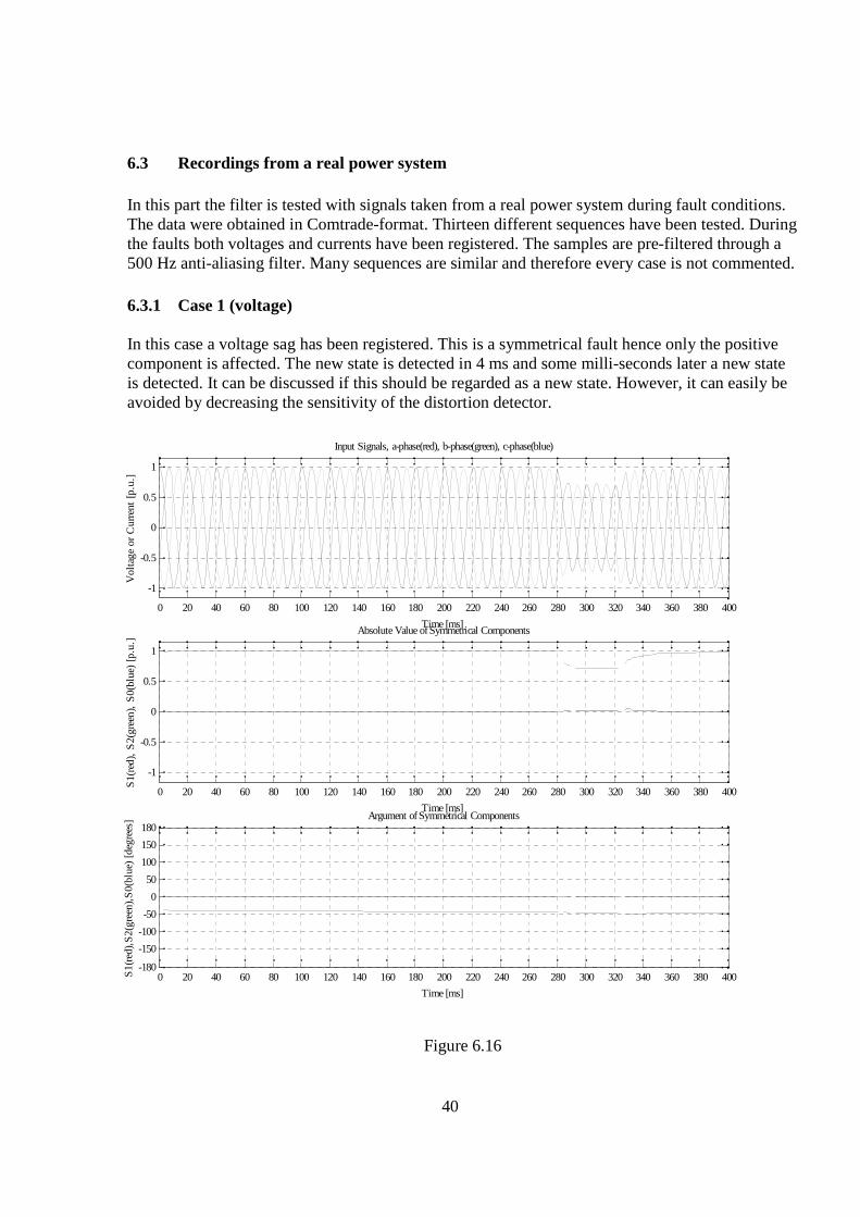
6.3 Recordings from a real power system In this part the filter is tested with signals taken from a real power system during fault conditions. The data were obtained in Comtrade-format. Thirteen different sequences have been tested. During the faults both voltages and currents have been registered. The samples are pre-filtered through a 500 Hz anti-aliasing filter. Many sequences are similar and therefore every case is not commented. 6.3.1 Case 1 (voltage) In this case a voltage sag has been registered. This is a symmetrical fault hence only the positive component is affected. The new state is detected in 4 ms and some milli-seconds later a new state is detected. It can be discussed if this should be regarded as a new state. However, it can easily be avoided by decreasing the sensitivity of the distortion detector.

0 20 40 60 80 100 120 140 160 180 200 220 240 260 280 300 320 340 360 380 400

-1

-0.5

0

0.5

1


Time [ms]

Vol

tage

or

Cur

rent

[p.

u.]

0 20 40 60 80 100 120 140 160 180 200 220 240 260 280 300 320 340 360 380 400

-1

-0.5

0

0.5

1


Time [ms]

S1(

red)

, S

2(gr

een)

, S

0(bl

ue)

[p.u

.]

0 20 40 60 80 100 120 140 160 180 200 220 240 260 280 300 320 340 360 380 400-180

-150

-100

-50

0

50

100

150


Time [ms]

S1(

red)

,S2(

gree

n),S

0(bl

ue)

[deg

rees

]

Figure 6.16

41

6.3.2 Case 1 (current) Simultaneous with the voltage sag, the magnitudes of the currents swell. The currents are not symmetrical during the fault and therefore the negative component appears. At the end of the fault period some zero sequence current appears. Again the big fluctuations of the arguments are due to that the argument is defined on the principal branch, see example 6.2.5.

0 20 40 60 80 100 120 140 160 180 200 220 240 260 280 300 320 340 360 380 400-6

-4

-2

0

2

4

6


Time [ms]

Vol

tage

or

Cur

rent

[p.

u.]

0 20 40 60 80 100 120 140 160 180 200 220 240 260 280 300 320 340 360 380 400-6

-4

-2

0

2

4

6


Time [ms]

S1(

red)

, S

2(gr

een)

, S

0(bl

ue)

[p.u

.]

0 20 40 60 80 100 120 140 160 180 200 220 240 260 280 300 320 340 360 380 400-180

-150

-100

-50

0

50

100

150


Time [ms]

S1(

red)

,S2(

gree

n),S

0(bl

ue)

[deg

rees

]

Figure 6.17

42

6.3.3 Case 2 (voltage) This case is similar to 6.3.1. The voltage sag is symmetrical and only the positive component is affected.

0 20 40 60 80 100 120 140 160 180 200 220 240 260 280 300 320 340 360 380 400

-1

-0.5

0

0.5

1


Time [ms]

Vol

tage

or

Cur

rent

[p.

u.]

0 20 40 60 80 100 120 140 160 180 200 220 240 260 280 300 320 340 360 380 400

-1

-0.5

0

0.5

1


Time [ms]

S1(

red)

, S

2(gr

een)

, S

0(bl

ue)

[p.u

.]

0 20 40 60 80 100 120 140 160 180 200 220 240 260 280 300 320 340 360 380 400-180

-150

-100

-50

0

50

100

150


Time [ms]

S1(

red)

,S2(

gree

n),S

0(bl

ue)

[deg

rees

]

Figure 6.18

43

6.3.4 Case 2 (current) Consequently, this case is similar to 6.3.2. The negative component appears during the fault and a zero sequence current appears immediately after the fault period. Again the big fluctuation of the argument is due to that the argument is defined on the principal branch, see example 6.2.5.

0 20 40 60 80 100 120 140 160 180 200 220 240 260 280 300 320 340 360 380 400

-3

-2

-1

0

1

2

3


Time [ms]

Vol

tage

or

Cur

rent

[p.

u.]

0 20 40 60 80 100 120 140 160 180 200 220 240 260 280 300 320 340 360 380 400

-3

-2

-1

0

1

2

3


Time [ms]

S1(

red)

, S

2(gr

een)

, S

0(bl

ue)

[p.u

.]

0 20 40 60 80 100 120 140 160 180 200 220 240 260 280 300 320 340 360 380 400-180

-150

-100

-50

0

50

100

150


Time [ms]

S1(

red)

,S2(

gree

n),S

0(bl

ue)

[deg

rees

]

Figure 6.19

44

6.3.5 Case 3 (voltage) This case is similar to 6.3.1, please refer that part for comments.

0 20 40 60 80 100 120 140 160 180 200 220 240 260 280 300 320 340 360 380 400 420 440

-1

-0.5

0

0.5

1


Time [ms]

Vol

tage

or

Cur

rent

[p.

u.]

0 20 40 60 80 100 120 140 160 180 200 220 240 260 280 300 320 340 360 380 400 420 440

-1

-0.5

0

0.5

1


Time [ms]

S1(

red)

, S

2(gr

een)

, S

0(bl

ue)

[p.u

.]

0 20 40 60 80 100 120 140 160 180 200 220 240 260 280 300 320 340 360 380 400 420 440-180

-150

-100

-50

0

50

100

150


Time [ms]

S1(

red)

,S2(

gree

n),S

0(bl

ue)

[deg

rees

]

Figure 6.20

45

6.3.6 Case 3 (current) This case is similar to 6.3.2, please refer that part for comments.

0 20 40 60 80 100 120 140 160 180 200 220 240 260 280 300 320 340 360 380 400 420 440

-20

-10

0

10

20


Time [ms]

Vol

tage

or

Cur

rent

[p.

u.]

0 20 40 60 80 100 120 140 160 180 200 220 240 260 280 300 320 340 360 380 400 420 440

-20

-10

0

10

20


Time [ms]

S1(

red)

, S

2(gr

een)

, S

0(bl

ue)

[p.u

.]

0 20 40 60 80 100 120 140 160 180 200 220 240 260 280 300 320 340 360 380 400 420 440-180

-150

-100

-50

0

50

100

150


Time [ms]

S1(

red)

,S2(

gree

n),S

0(bl

ue)

[deg

rees

]

Figure 6.21

46

6.3.7 Case 4 (voltage) In this case only the b and c-phases sag during the fault. This is an unsymmetrical fault that is proved by the negative component occurring during the fault.

0 20 40 60 80 100 120 140 160 180 200 220 240 260 280 300 320 340 360 380 400 420 440

-1

-0.5

0

0.5

1


Time [ms]

Vol

tage

or

Cur

rent

[p.

u.]

0 20 40 60 80 100 120 140 160 180 200 220 240 260 280 300 320 340 360 380 400 420 440

-1

-0.5

0

0.5

1


Time [ms]

S1(

red)

, S

2(gr

een)

, S

0(bl

ue)

[p.u

.]

0 20 40 60 80 100 120 140 160 180 200 220 240 260 280 300 320 340 360 380 400 420 440-180

-150

-100

-50

0

50

100

150


Time [ms]

S1(

red)

,S2(

gree

n),S

0(bl

ue)

[deg

rees

]

Figure 6.22

47

6.3.8 Case 4 (current) In this case the negative component is present almost all the time in the argument plot indicating an unsymmetrical condition. In the program the absolute value of a component has to exceed a threshold value in order to calculate the argument of the same component. Otherwise the program would calculate arguments even for infinite small absolute values of the components. In this case maybe the threshold value was set too low. The absolute values of the components look accurate though.

0 20 40 60 80 100 120 140 160 180 200 220 240 260 280 300 320 340 360 380 400 420 440

-30

-20

-10

0

10

20

30


Time [ms]

Vol

tage

or

Cur

rent

[p.

u.]

0 20 40 60 80 100 120 140 160 180 200 220 240 260 280 300 320 340 360 380 400 420 440

-30

-20

-10

0

10

20

30


Time [ms]

S1(

red)

, S

2(gr

een)

, S

0(bl

ue)

[p.u

.]

0 20 40 60 80 100 120 140 160 180 200 220 240 260 280 300 320 340 360 380 400 420 440-180

-150

-100

-50

0

50

100

150


Time [ms]

S1(

red)

,S2(

gree

n),S

0(bl

ue)

[deg

rees

]

Figure 6.23

48


0 20 40 60 80 100 120 140 160 180 200 220 240 260 280 300 320 340 360 380 400 420 440

-1

-0.5

0

0.5

1


Time [ms]

Vol

tage

or

Cur

rent

[p.

u.]

0 20 40 60 80 100 120 140 160 180 200 220 240 260 280 300 320 340 360 380 400 420 440

-1

-0.5

0

0.5

1


Time [ms]

S1(

red)

, S

2(gr

een)

, S

0(bl

ue)

[p.u

.]

0 20 40 60 80 100 120 140 160 180 200 220 240 260 280 300 320 340 360 380 400 420 440-180

-150

-100

-50

0

50

100

150


Time [ms]

S1(

red)

,S2(

gree

n),S

0(bl

ue)

[deg

rees

]

Figure 6.24

49

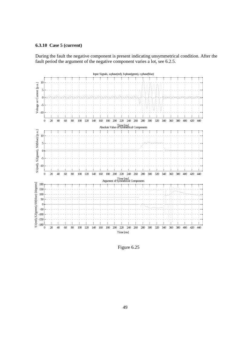
6.3.10 Case 5 (current) During the fault the negative component is present indicating unsymmetrical condition. After the fault period the argument of the negative component varies a lot, see 6.2.5.

0 20 40 60 80 100 120 140 160 180 200 220 240 260 280 300 320 340 360 380 400 420 440

-10

-5

0

5

10


Time [ms]

Vol

tage

or

Cur

rent

[p.

u.]

0 20 40 60 80 100 120 140 160 180 200 220 240 260 280 300 320 340 360 380 400 420 440

-10

-5

0

5

10


Time [ms]

S1(

red)

, S

2(gr

een)

, S

0(bl

ue)

[p.u

.]

0 20 40 60 80 100 120 140 160 180 200 220 240 260 280 300 320 340 360 380 400 420 440-180

-150

-100

-50

0

50

100

150


Time [ms]

S1(

red)

,S2(

gree

n),S

0(bl

ue)

[deg

rees

]

Figure 6.25

50

6.3.11 Case 6 (voltage) In this case the a-phase sags during the fault making it look like a single line-to-ground fault. Hence, both positive, negative and zero components are affected during the fault period.

0 20 40 60 80 100 120 140 160 180 200 220 240 260 280 300 320 340 360 380 400 420 440

-1

-0.5

0

0.5

1


Time [ms]

Vol

tage

or

Cur

rent

[p.

u.]

0 20 40 60 80 100 120 140 160 180 200 220 240 260 280 300 320 340 360 380 400 420 440

-1

-0.5

0

0.5

1


Time [ms]

S1(

red)

, S

2(gr

een)

, S

0(bl

ue)

[p.u

.]

0 20 40 60 80 100 120 140 160 180 200 220 240 260 280 300 320 340 360 380 400 420 440-180

-150

-100

-50

0

50

100

150


Time [ms]

S1(

red)

,S2(

gree

n),S

0(bl

ue)

[deg

rees

]

Figure 6.26

51


0 20 40 60 80 100 120 140 160 180 200 220 240 260 280 300 320 340 360 380 400 420 440

-1

-0.5

0

0.5

1


Time [ms]

Vol

tage

or

Cur

rent

[p.

u.]

0 20 40 60 80 100 120 140 160 180 200 220 240 260 280 300 320 340 360 380 400 420 440

-1

-0.5

0

0.5

1


Time [ms]

S1(

red)

, S

2(gr

een)

, S

0(bl

ue)

[p.u

.]

0 20 40 60 80 100 120 140 160 180 200 220 240 260 280 300 320 340 360 380 400 420 440-180

-150

-100

-50

0

50

100

150


Time [ms]

S1(

red)

,S2(

gree

n),S

0(bl

ue)

[deg

rees

]

Figure 6.27

52

6.3.13 Case 8 (current) This case is similar to 6.3.2, please refer that part for comments.

0 20 40 60 80 100 120 140 160 180 200 220 240 260 280 300 320 340 360 380 400 420 440

-3

-2

-1

0

1

2

3


Time [ms]

Vol

tage

or

Cur

rent

[p.

u.]

0 20 40 60 80 100 120 140 160 180 200 220 240 260 280 300 320 340 360 380 400 420 440

-3

-2

-1

0

1

2

3


Time [ms]

S1(

red)

, S

2(gr

een)

, S

0(bl

ue)

[p.u

.]

0 20 40 60 80 100 120 140 160 180 200 220 240 260 280 300 320 340 360 380 400 420 440-180

-150

-100

-50

0

50

100

150


Time [ms]

S1(

red)

,S2(

gree

n),S

0(bl

ue)

[deg

rees

]

Figure 6.28

53

7 Conclusions and Suggestions for Future Work Conclusions Symmetrical components are widely used in relay protection systems to detect abnormal conditions in a power system. In the relay protection industry there is a demand for an ultra fast estimation method of symmetrical components. An estimation time of 5 ms or less is desirable. Most methods used today utilize one cycle Fourier filtering algorithms, resulting in an estimation time of at least one cycle. In this work a method based on variable window size, the least squares method and sample prediction has been developed. The least squares method is used to suppress noise and harmonics of the fundamental frequency. During steady state in the power system the window size is equal to the number of samples per fundamental frequency cycle. If for instance the fundamental frequency is 50 Hz, the twenty most recent samples are used for the estimation of the symmetrical components. When a fault is detected the window will be minimized and all pre-fault samples will be discarded. After the fault is detected the window will be built up step by step until it reaches full size again. The variable window size enables fast estimations after a fault has occurred with better accuracy of the estimates as the window size grows. The filter algorithm is implemented and verified in Matlab. The sampling frequency of the input signals is 1000 Hz that is standard in ABB relay protection systems. It is assumed that the frequency of the input signals is known. Outliers in the input samples have not been considered either since in real applications the input signals already are lowpass filtered. It is also assumed that the fault time is longer than the estimation time. Simulations have been made with signals created in Matlab and Simulink and with real signals measured from a real power system. The results show that it is possible to detect a fault and estimate new symmetrical components in 4 ms with exact results if the signals are undisturbed and if they make a step change to a new stationary state. In reality the signals are disturbed with noise and harmonics and after a fault the signals contain a lot of transients. In general noisy signals do not affect the possibility to detect a fault, but the post-fault transients affects the accuracy of the estimates. If good accuracy is needed it might be needed to wait some samples before starting the estimation. This increases the estimation time of course. Here the filter has been adjusted to find a good balance between sensitivity, security to false trips, speed and accuracy. Same settings have been used both for signals representing currents and voltages. This is a compromise and in order to increase the performance, the filter might be individual set for each application. It might also be necessary to high-pass filter the input signals to eliminate possible DC-components since DC-components most likely will disturb the estimates. Suggestions for Future Work These results are achieved with simulations in Matlab and might not be directly transferable to a real-time implementation. It is for instance hard to predict exactly how the input signals will look like and all other problems that possibly will occur. A real-time implementation will require both hardware design and probably new software design. This would be the natural continuation of this study but that is beyond the scope of this work though. As mentioned before, high-pass pre-filtering of the input signals might be necessary. It may most likely be possible to write the filter algorithm in a more efficient way, especially the least-squares method. Now the summation starts

54

all over each time a new sample enters the filter, probably it is more efficient to store the last sum and add the new sample to it instead.

55

8 References

1. A.J. Degens: Microprocessor-implemented digital filters for the calculation of symmetrical components, IEE PROC, Vol. 129, Pt. C, No. 3, MAY 1982

2. S.R. Kolla: Block pulse functions based algorithm for symmetrical components calculation, IEE PROC, Vol.135, Pt. C, No.6, NOVEMBER 1988

3. T.Lobos: Fast estimation of symmetrical components in real time, IEE PROCEEDINGS-C,

Vol. 139, No. 1, JANUARY 1992

4. K.M. El-Naggar: A fast method for identification of symmetrical components for power system protection, Electrical Power and Energy Systems 23(2001) 813-817

5. Chunlin Li, F.P. Dawson: A new algorithm for fast retrieval of sequence components in 3-

phase networks, 0-7803-7156-9/02 2002 IEEE

6. Lj. A. Kojovic, J.F. Witte: Improved Protection Systems using Symmetrical Components, 0-7803-7285-9/01 © 2001 IEEE

7. C.L. Fortescue: Method of Symmetrical Co-ordinates Applied to the Solution of Polyphase

Networks, AIEE Transactions, vol. 37, pt. II, pp. 1027-1140, June 1918

8. J. Duncan Glover, Mulukutla Sarma: Power System Analysis and Design, PWS Publishing Company, 1994

9. Sture Lindahl: Estimation of Symmetrical Components, 2002

10. Gunnar Blom, Björn Holmquist: Statistikteori med tillämpningar, Studentlitteratur, 1998

11. Karl J. Åström, Björn Wittenmark: Computer Controlled Systems, Theory and Design,

Prentice-Hall Information and System Sciences Series, 1984

12. Gunnar Elfving, m.fl.: ABB HANDBOK ELKRAFT, Asea Distribution AB, Västerås, 1987

13. Sven Spanne: Konkret analys, Matematiska Institutionen, Lunds Tekniska Högskola, 1997

56

9 Appendix %%%%%%%%%%%%%%%%%%%%%%%%%%%%%%%%%%%%%%%%%%%%%%%%%%%%%%%%%%%%%% % Program for fast estimation of symmetrical components % % Jonas Johansson 2002 % %%%%%%%%%%%%%%%%%%%%%%%%%%%%%%%%%%%%%%%%%%%%%%%%%%%%%%%%%%%%%% clear format short %%%%%%%%% Generating input signals %%%%%%%%%%%%%%%%%%%%%%%%%%%%%%%%%%%%%%%%%%%%%%%%%%%%% load safhtI; % Load input signals from Comtrade-files load sbfhtI; load scfhtI; pu = max(safhtI(1:100)); % determine per unit base sa = (safhtI’)/pu; % convert input signals to p.u. sb = (sbfhtI’)/pu; sc = (scfhtI’)/pu; %simugen2; % Load input signals from Simulink %Ts = 50e-6; %sim(’simugen2’); %load simc; %load sima; %load sima; %sa = simc(1:end,1); %sb = simc(1:end,2); %sc = simc(1:end,3); t = 0:1/1000:0.7; % Create own input signals fas = pi/6; frek = 50; %sa = 0.5*sin(2*pi*frek*t + fas)+0*sin(2*pi*2*frek*t + fas)+0.1*sin(2*pi*3*frek*t + fas)+0*sin(2*pi*4*frek*t + fas);%+0.108*sin(2*pi*4*frek*t + fas)+0.08*sin(2*pi*5*frek*t + fas);% + 0.01*randn(size(t));%+ 0.2*sin(2*pi*150*t + fas); %sb = 0.5*sin(2*pi*frek*t - 2*pi/3 + fas)+0*sin(2*pi*2*frek*t - 2*pi/3 + fas)+0.1*sin(2*pi*3*frek*t - 2*pi/3 + fas)+0*sin(2*pi*4*frek*t - 2*pi/3 + fas);%+0.108*sin(2*pi*4*frek*t - 2*pi/3 + fas)+0.08*sin(2*pi*5*frek*t - 2*pi/3 + fas);% + 0.01*randn(size(t)); %0.2*sin(2*pi*150*t - 2*pi/3 + fas);% %sc = 0.5*sin(2*pi*frek*t - 4*pi/3 + fas)+0*sin(2*pi*2*frek*t - 4*pi/3 + fas)+0.1*sin(2*pi*3*frek*t - 4*pi/3 + fas)+0*sin(2*pi*4*frek*t - 4*pi/3 + fas);%+0.108*sin(2*pi*4*frek*t - 4*pi/3 + fas);+0.08*sin(2*pi*5*frek*t - 4*pi/3 + fas);% + 0.01*randn(size(t));% + 0.2*sin(2*pi*150*t - 4*pi/3 + fas); %%%%%%%%% Estimation of symmetrical components %%%%%%%%%%%%%%%%%%%%%%%%%%%%%%%%%%%%%%%% sap = sa(1); % Predicted sample of a-phase, initially % set to equal the first sample sbp = sb(1); % Predicted sample of b-phase, initially

% set to equal the first sample scp = sc(1); % Predicted sample of c-phase, initially

% set to equal the first sample % k = current sample in the window G = 5; % Gain factor for adjustment of deviation

% limit for residuals h = 1; % First sample in the window n = 1; % Last sample in the window p = 1; % Index for estimated components vector f = 1; % Index for residual vector for standard

% deviation calculation M = 0; % Window size lima = 3; % Deviation limit for residuals of

57

% a-phase, initially set to 3 limb = 3; % Deviation limit for residuals of

% b-phase, initially set to 3 limc = 3; % Deviation limit for residuals of

% c-phase, initially set to 3 range = 1.1*max(abs(sb)); % Adjust plot window size for l = 1:450 % an infinite loop in reality f1f1=0;f1f2=0;f1f3=0;f1f4=0;f1f5=0;f1f6=0; % Reset the A-matrix before building up

% the window size f2f1=0;f2f2=0;f2f3=0;f2f4=0;f2f5=0;f2f6=0; f3f1=0;f3f2=0;f3f3=0;f3f4=0;f3f5=0;f3f6=0; f4f1=0;f4f2=0;f4f3=0;f4f4=0;f4f5=0;f4f6=0; f5f1=0;f5f2=0;f5f3=0;f5f4=0;f5f5=0;f5f6=0; f6f1=0;f6f2=0;f6f3=0;f6f4=0;f6f5=0;f6f6=0; F1F1=0;F1F2=0;F1F3=0;F1F4=0;F1F5=0;F1F6=0; F2F1=0;F2F2=0;F2F3=0;F2F4=0;F2F5=0;F2F6=0; F3F1=0;F3F2=0;F3F3=0;F3F4=0;F3F5=0;F3F6=0; F4F1=0;F4F2=0;F4F3=0;F4F4=0;F4F5=0;F4F6=0; F5F1=0;F5F2=0;F5F3=0;F5F4=0;F5F5=0;F5F6=0; F6F1=0;F6F2=0;F6F3=0;F6F4=0;F6F5=0;F6F6=0; F1Y=0;F2Y=0;F3Y=0;F4Y=0;F5Y=0;F6Y=0; f1y=0;f2y=0;f3y=0;f4y=0;f5y=0;f6y=0; % Reset the B-matrix before building up

% the window size z = 0; % Help variable to count number of loop

% runs p = p+1; sadev = (sap-sa(n)); % Calculate a-phase residuals between % predicted sample and actual sample sbdev = (sbp-sb(n)); % Calculate b-phase residuals between % predicted sample and actual sample scdev = (scp-sc(n)); % Calculate c-phase residuals between % predicted sample and actual sample for k = h:n % Create A and B-matrix elements, least % squares method if abs(sadev)>lima | abs(sbdev)>limb | abs(scdev)>limc % Fault detector h = n+1; % Start up new window at next sample M = 0; % Minimize window size sares = [sares(end:end)]; % Minimize a-phase residual vector to a % 1x1 matrix sares = 0; % Reset the element sbres = [sbres(end:end)]; % Minimize b-phase residual vector to a % 1x1 matrix sbres = 0; % Reset the element scres = [scres(end:end)]; % Minimize c-phase residual vector to a % 1x1 matrix scres = 0; % Reset the element f = 0; break % Exit the loop end

Ok = (k-1)*2*pi*frek*0.001; % Help variables to make the A-matrix % more foreseeable

f1 = cos(Ok); f2 = sin(Ok); f3 = cos(Ok-2*pi/3); f4 = sin(Ok-2*pi/3); f5 = cos(Ok-4*pi/3); f6 = sin(Ok-4*pi/3);

58

F1F1 = f1*f1+f3*f3+f5*f5; % A-matrix elements f1f1 = f1f1 + F1F1; F1F2 = f2*f1+f4*f3+f6*f5; f1f2 = f1f2 + F1F2; F1F3 = f1*f1+f5*f3+f3*f5; f1f3 = f1f3 + F1F3; F1F4 = f2*f1+f6*f3+f4*f5; f1f4 = f1f4 + F1F4; F1F5 = f1*f1+f1*f3+f1*f5; f1f5 = f1f5 + F1F5; F1F6 = f2*f1+f2*f3+f2*f5; f1f6 = f1f6 + F1F6; F2F1 = f1*f2+f3*f4+f5*f6; f2f1 = f2f1 + F2F1; F2F2 = f2*f2+f4*f4+f6*f6; f2f2 = f2f2 + F2F2; F2F3 = f1*f2+f5*f4+f3*f6; f2f3 = f2f3 + F2F3; F2F4 = f2*f2+f6*f4+f4*f6; f2f4 = f2f4 + F2F4; F2F5 = f1*f2+f1*f4+f1*f6; f2f5 = f2f5 + F2F5; F2F6 = f2*f2+f2*f4+f2*f6; f2f6 = f2f6 + F2F6; F3F1 = f1*f1+f3*f5+f5*f3; f3f1 = f3f1 + F3F1; F3F2 = f2*f1+f4*f5+f6*f3; f3f2 = f3f2 + F3F2; F3F3 = f1*f1+f5*f5+f3*f3; f3f3 = f3f3 + F3F3; F3F4 = f2*f1+f6*f5+f4*f3; f3f4 = f3f4 + F3F4; F3F5 = f1*f1+f1*f5+f1*f3; f3f5 = f3f5 + F3F5; F3F6 = f2*f1+f2*f5+f2*f3; f3f6 = f3f6 + F3F6; F4F1 = f1*f2+f3*f6+f5*f4; f4f1 = f4f1 + F4F1; F4F2 = f2*f2+f4*f6+f6*f4; f4f2 = f4f2 + F4F2; F4F3 = f1*f2+f5*f6+f3*f4; f4f3 = f4f3 + F4F3; F4F4 = f2*f2+f6*f6+f4*f4; f4f4 = f4f4 + F4F4; F4F5 = f1*f2+f1*f6+f1*f4; f4f5 = f4f5 + F4F5; F4F6 = f2*f2+f2*f6+f2*f4; f4f6 = f4f6 + F4F6; F5F1 = f1*f1+f3*f1+f5*f1; f5f1 = f5f1 + F5F1; F5F2 = f2*f1+f4*f1+f6*f1; f5f2 = f5f2 + F5F2; F5F3 = f1*f1+f5*f1+f3*f1; f5f3 = f5f3 + F5F3; F5F4 = f2*f1+f6*f1+f4*f1; f5f4 = f5f4 + F5F4; F5F5 = f1*f1+f1*f1+f1*f1; f5f5 = f5f5 + F5F5; F5F6 = f2*f1+f2*f1+f2*f1;

59

f5f6 = f5f6 + F5F6; F6F1 = f1*f2+f3*f2+f5*f2; f6f1 = f6f1 + F6F1; F6F2 = f2*f2+f4*f2+f6*f2; f6f2 = f6f2 + F6F2; F6F3 = f1*f2+f5*f2+f3*f2; f6f3 = f6f3 + F6F3; F6F4 = f2*f2+f6*f2+f4*f2; f6f4 = f6f4 + F6F4; F6F5 = f1*f2+f1*f2+f1*f2; f6f5 = f6f5 + F6F5; F6F6 = f2*f2+f2*f2+f2*f2; f6f6 = f6f6 + F6F6; F1Y = f1*sa(k)+f3*sb(k)+f5*sc(k); % B-matrix elements f1y = f1y + F1Y; F2Y = f2*sa(k)+f4*sb(k)+f6*sc(k); f2y = f2y + F2Y; F3Y = f1*sa(k)+f5*sb(k)+f3*sc(k); f3y = f3y + F3Y; F4Y = f2*sa(k)+f6*sb(k)+f4*sc(k); f4y = f4y + F4Y; F5Y = f1*sa(k)+f1*sb(k)+f1*sc(k); f5y = f5y + F5Y; F6Y = f2*sa(k)+f2*sb(k)+f2*sc(k); f6y = f6y + F6Y; z = z+1; % Loop count end A = [f1f1 f1f2 f1f3 f1f4 f1f5 f1f6; % Create the A-matrix f2f1 f2f2 f2f3 f2f4 f2f5 f2f6; f3f1 f3f2 f3f3 f3f4 f3f5 f3f6; f4f1 f4f2 f4f3 f4f4 f4f5 f4f6; f5f1 f5f2 f5f3 f5f4 f5f5 f5f6; f6f1 f6f2 f6f3 f6f4 f6f5 f6f6]; B = [f1y f2y f3y f4y f5y f6y]’; % Create the B-matrix if z<=2 % Calculate symmetrical components when

% window size is two or bigger X = [NaN NaN NaN NaN NaN NaN]’; else X = (A\B)’; % Determine A1,B1,A2,B2,A0,A0 end absS1(p) = abs(X(2)+i*X(1)); % Calculate absolute value of positive

% sequence component absS2(p) = abs(X(4)+i*X(3)); % Calculate absolute value of negative

% sequence component absS0(p) = abs(X(6)+i*X(5)); % Calculate absolute value of zero

% sequence component if absS1(p) < 1e-1 % Calculate argument of positive sequence

% component argS1(p) = 0; else argS1(p) = angle(X(2)+i*X(1))*180/pi; end if absS2(p) < 3e-1 % Calculate argument of negative sequence

% component argS2(p) = 0;

60

else argS2(p) = angle(X(4)+i*X(3))*180/pi; end if absS0(p) < 1e-1 % Calculate argument of zero sequence

% component argS0(p) = 0; else argS0(p) = angle(X(6)+i*X(5))*180/pi; end if M < 20 % Increase window size if it has not

% reached full size n = n+1; end if M == 20 % When full window size, "move" the

% window one sample to the right M = 19; h = h+1; % Discard the oldest sample n = n+1; % Put in the most recent sample in the

% window end M = M+1; %%%%%%%% Prediction of next sample %%%%%%%%%%%%%%%%%%%%%%%%%%%%%%%%%%%%%%%%%%%%%%%%%%%%% Okp = (k)*2*pi*frek*0.001;

sap = X(1)*cos(Okp)+X(2)*sin(Okp) + X(3)*cos(Okp)+X(4)*sin(Okp) + X(5)*cos(Okp)+X(6)*sin(Okp); % Predict next a-phase sample sapplot(p) = sap; % plot vector for predicted a-phase

% samples sbp = X(1)*cos(Okp-2*pi/3)+X(2)*sin(Okp-2*pi/3) + X(3)*cos(Okp-4*pi/3)+X(4)*sin(Okp- 4*pi/3) + X(5)*cos(Okp)+X(6)*sin(Okp); % Predict next b-phase sample

sbpplot(p) = sbp; % plot vector for predicted b-phase % samples

scp = X(1)*cos(Okp-4*pi/3)+X(2)*sin(Okp-4*pi/3) + X(3)*cos(Okp-2*pi/3)+X(4)*sin(Okp- 2*pi/3) + X(5)*cos(Okp)+X(6)*sin(Okp); % Predict next c-phase sample

scpplot(p) = scp; % plot vector for predicted c-phase % samples

%%%%%%%% Determination of deviation limit %%%%%%%%%%%%%%%%%%%%%%%%%%%%%%%%%%%%%%%%%%%%%% if M > 2 f = f+1; sares(f) = sadev; % Create a residual vector for the a-phase sbres(f) = sbdev; % Create a residual vector for the b-phase scres(f) = scdev; % Create a residual vector for the c-phase saresplot(p) = sadev; % Create a plot vector for the a-phase

% residuals sbresplot(p) = sbdev; % Create a plot vector for the b-phase

% residuals scresplot(p) = scdev; % Create a plot vector for the c-phase

% residuals if size(sares) == [1 21] % When full window size, discard the

% oldest residual sares = [sares(2:end)]; sbres = [sbres(2:end)]; scres = [scres(2:end)]; f = f-1; end sares = sares(find(~isnan(sares))); % Remove NaN’s from the vector

61

if size(sares) > [0 0] lima = G*std(sares); % Determine deviation limit if lima < 1e-3 % Avoid too narrow limit to avoid false

% trips lima = 0.1; end end sbres = sbres(find(~isnan(sbres))); % Remove NaN’s from the vector if size(sbres) > [0 0] limb = G*std(sbres); % Determine deviation limit if limb < 1e-3 % Avoid too narrow limit to avoid false

% trips limb = 0.1; end end scres = scres(find(~isnan(scres))); % Remove NaN’s from the vector if size(scres) > [0 0] limc = G*std(scres); % Determine deviation limit if limc < 1e-3 % Avoid too narrow limit to avoid false

% trips limc = 0.1; end end if M <6 % Increase the deviation limit for the

% first six samples following a fault lima = 3; % to avoid a new fault detection during

% the transient period limb = 3; limc = 3; end end end %%%%%%%%%% Plots %%%%%%%%%%%%%%%%%%%%%%%%%%%%%%%%%%%%%%%%%%%%%%%%%%%%%%%%%%%%%%%%%%%%%%% figsize = [250, -350, 800, 1200]; figure(’Pos’,figsize); % Plot of input signals subplot(3,1,1) plot(t(1:p),sa(1:p),’r’,t(1:p),sb(1:p),’g’,t(1:p),sc(1:p),’b’) title(’Input Signals, a-phase(red), b-phase(green), c-phase(blue)’,’FontSize’,8); xlabel(’Time [ms]’,’FontSize’,8); ylabel(’Voltage or Current [p.u.]’,’FontSize’,8); set(gca,’FontSize’,8); axis([0 0.45 -range range]); set(gca,’XTick’,0:0.02:0.45) set(gca,’XTickLabel’,{’0’,’20’,’40’,’60’,’80’,’100’,’120’,’140’,’160’,’180’,’200’,’220’,’240’,’260’,’280’,’300’,’320’,’340’,’360’,’380’,’400’,’420’,’440’,’460’}) grid on subplot(3,1,2) % Plot absolute value of S1, S2, S0 plot(t(1:p),absS1(1:p),’r’,t(1:p),absS2(1:p),’g’,t(1:p),absS0(1:p),’b’) title(’Absolute Value of Symmetrical Components’,’FontSize’,8); xlabel(’Time [ms]’,’FontSize’,8); ylabel(’S1(red), S2(green), S0(blue) [p.u.]’,’FontSize’,8); set(gca,’FontSize’,8); axis([0 0.45 -range range]); set(gca,’XTick’,0:0.02:0.45) set(gca,’XTickLabel’,{’0’,’20’,’40’,’60’,’80’,’100’,’120’,’140’,’160’,’180’,’200’,’220’,’240’,’260’,’280’,’300’,’320’,’340’,’360’,’380’,’400’,’420’,’440’,’460’}) grid on

62

subplot(3,1,3) % Plot argument of S1, S2, S0 plot(t(1:p),argS1(1:p),’r’,t(1:p),argS2(1:p),’g’,t(1:p),argS0(1:p),’b’) title(’Argument of Symmetrical Components’,’FontSize’,8); xlabel(’Time [ms]’,’FontSize’,8); ylabel(’S1(red),S2(green),S0(blue) [degrees]’,’FontSize’,8); set(gca,’FontSize’,8); set(gca,’YTick’,-200:50:200) set(gca,’YTickLabel’,{’-180’,’-150’,’-100’,’-50’,’0’,’50’,’100’,’150’,’180’}) axis([0 0.45 -200 200]); set(gca,’XTick’,0:0.02:0.45) set(gca,’XTickLabel’,{’0’,’20’,’40’,’60’,’80’,’100’,’120’,’140’,’160’,’180’,’200’,’220’,’240’,’260’,’280’,’300’,’320’,’340’,’360’,’380’,’400’,’420’,’440’,’460’}) grid on figure(4) % Plot predicted input signals plot(t(1:p),sapplot(1:p),’r’,t(1:p),sbpplot(1:p),’g’,t(1:p),scpplot(1:p),’b’) xlabel(’Time [s]’,’FontSize’,10); ylabel('Predikterade fassignaler[a(röd), b(blå), c(grön)]'); axis([0 0.45 -range range]); grid on figure(5) % Plot residuals plot(t(1:p),saresplot(1:p),'r',t(1:p),sbresplot(1:p),'g',t(1:p),scresplot(1:p),'b') xlabel('Time[s]','FontSize',10); ylabel('Residualer[a(röd), b(blå), c(grön)]'); axis([0 0.45 -0.15 0.15]);

department of industrial electrical engineering and

Documents