Department of Economics Working Paper Series

Monetary Policy in a Portfolio Balance Model with EndogenousPhysical Capital

Habib AhmedNational University of Singapore

C. Paul HallwoodUniversity of Connecticut

Stephen M. MillerUniversity of Connecticut

Working Paper 1997-08

July 1997

341 Mansfield Road, Unit 1063Storrs, CT 06269–1063Phone: (860) 486–3022Fax: (860) 486–4463http://www.econ.uconn.edu/

AbstractWe develop a portfolio balance model with real capital accumulation. The

introduction of real capital as an asset as well as a good produced and demandedby firms enriches extant portfolio balance models of exchange rate determination.We show that expansionary monetary policy causes exchange rate overshooting,not once, but twice; the secondary repercussion comes through the reaction offirms to changed asset prices and the firms’ decisions to invest in real capital. Themodel sheds further light on the volatility of real and nominal exchange rates, andit suggests that changes in corporate sector profitability may affect exchange ratesthrough portfolio diversification in corporate securities.

Journal of Economic Literature Classification: F31, F32

2

1. Introduction

Even though capital goods constitute a large percentage of total trade and

empirical studies show that investment affects the long-term current account balance,1

few portfolio balance models incorporate investment in physical capital (Krueger, 1983).

Rather, these models typically postulate a fixed capital stock, and consider only financial

assets in the portfolios of households (e.g., Allen and Kenen, 1980, Branson, 1978,

Dornbusch and Fischer, 1980, Dornbusch, 1975, chapter 5, Genberg and Kierzkowski,

1979, Isard, 1977, Kouri, 1976, and Rodrigues, 1980).2 A similar state of affairs holds for

empirical tests of portfolio balance models (e.g., Hooper and Morton 1983, and Frankel

1983).

The omission of investment in models that consider the current account poses a

theoretical problem, since the current account is defined as the (ex-post) difference

between saving and investment. By considering investment as fixed, fluctuations in the

current account correspond only to adjustments in national saving. Those few models that

do incorporate capital do not consider an array of assets. For example, Dornbusch (1975,

chapter 6) includes the capital stock in a portfolio balance model, but does not consider

domestic (private or government) bonds. Furthermore, capital, a nontraded good in his

model, does not affect the current account directly. In our model, however, physical

capital is a traded good and, as such, affects the current account.

The current account does have an important role to play in existing portfolio

balance models. That is, changes in the current account affect income and wealth that, in

turn, affect consumption, money demand, the equilibrium exchange rate, domestic bond

prices, and, given the usual risk aversion assumption, domestic wealthholders' preferences

between holding domestic and foreign government bonds. But what the extant portfolio

balance literature fails to consider is any effect of changes in asset prices, including the

exchange rate, on the level of domestic real corporate investment and the size of the

capital stock. And, of course, there is no consideration of feedbacks from changes in the

level of corporate investment to asset prices and the current account. Furthermore, as we

note in our conclusion, because they ignore the effect of changes in the real exchange rate

1 In a sample of 82 countries, capital imports represented about 30 percent of total imports (Serven, 1995).Dar and Amirkhalkhali (1991) and Sachs (1981, 1983) show the effects of investment on the currentaccount.2Some current account models incorporate investment in physical capital, but these models do notconsider asset markets (e.g., Kouri, 1978, Sachs, 1981, and Ruffin, 1979). Some monetary models alsoconsider capital, but the exchange rate is not an asset price as in portfolio balance models (e.g., Connollyand Taylor, 1976, and Frenkel and Rodriguez, 1975).

3

on the level of private sector profits and corporate investment, extant portfolio balance

models may incorrectly perceive the effect of an increase in a country's money supply, and

consequent corporate sector profitability, on currency risk premia.

Since we think that feedbacks from changes in the level of investment to asset

prices and the current account are important in a properly specified model, we extend a

representative portfolio balance model, that of Hallwood and MacDonald (1994, chapter

10), by adding endogenous physical capital. Endogenous physical capital in a portfolio

balance model differs from financial assets because it is produced, supplied, and demanded

by firms. Such investment directly links the asset and goods markets, and this is a different

emphasis than is found in other portfolio balance models for, as Allen and Kenen (1978)

and Hallwood and MacDonald (1994) note, the goods market is only indirectly linked to

the asset market through the exchange rate; no direct link exists. We also show, and

emphasize, how endogenous physical capital affects both the current and capital accounts

of the balance of payments.

The most important implication of endogenous physical capital is that innovations

in monetary policy have longer-lasting and even more volatile effects on the time-path of

equilibrium exchange rates than they do in existing portfolio balance models. Thus, by

pointing to a previously over-looked dynamic specification, our analytical results may help

to explain the poor empirical performance of earlier portfolio balance models for, as

Meese and Rogoff (1983) note, in out of sample exchange rate predictions, portfolio

balance models are unable to beat a random walk.

In the interest of clarity, we make certain simplifying assumptions in addition to

those usually made in the portfolio balance model literature. First, physical capital is

rendered endogenous in the context of just two time periods, periods t and t+1. The

advantage of this is to avoid the complication of using discounted values. Second, we

assume that capital fully depreciates over the course of a single time period, which defines

the outstanding capital stock to equal the current period's level of investment. The

advantage of this is again one of simplification. Third, while the novelty of this paper is to

render endogenous the stock of physical capital, we think that our most important results

stand even making the assumption that the rates of interest on domestic government and

corporate bonds are at all times equal. That is, we assume that these bonds are perfect

substitutes.

The rest of the paper is organized as follows: section 2 describes our model;

section 3 illustrates how exchange rate volatility is engendered following a monetary

innovation; and the final section draws conclusions.

4

2. The Model

Consider a small open economy producing three goods -- traded and nontraded

consumption goods, and a traded capital good (T, N, and K, respectively). The household

sector's wealth consists of money (M), domestic government and private bonds (Bh and

Bk, respectively), and foreign government bonds (F).3 Private bonds finance investment in

capital. Since capital goods are produced by firms, we first consider the demand for and

supply of capital as a good. Then we discuss the demand for and supply of capital as an

asset in the asset market.

Demand for and Supply of Capital

Assume that firms make investment decisions and that all capital fully depreciates

within the period. Thus, the capital stock equals investment.4 The demand for physical

capital emerges from the profit maximization decisions of firms as in, inter alia, Frenkel

and Rodriguez (1975), Dornbusch (1975), and Sachs (1981). Once firms know their

demand for capital, they float bonds to finance this demand. We assume that the rate of

interest at which firms borrow equals that of the domestic government bond, r, implying

that government bonds and bonds supplied by firms are perfect substitutes.

The price of the nontraded good (PN) clears the market and, given the assumption

of a small open economy, the prices of the traded consumption (PT) and capital (PK) goods

equal prices, adjusting for the exchange rate, in the rest of the world. That is,

(1) PT = EP*T, and PK = EP*K,

where E is the nominal exchange rate defined as the domestic currency price of a unit of

foreign exchange, and P*T and P*K are exogenously given prices of the traded

consumption and capital goods in foreign currency. For given expected values of r, PN, E,

and P*i (i = T, K), the demand for capital emerges from profit maximization as shown

below. The nature of expectations appears in due course.

Production of good i (i = T, N, and K) responds positively to the amount of capital

used as follows:

(2) Yi = yi (Ki), yiK > 0,

where yiK is the marginal physical product of capital in sector i. Firms in sector i maximize

profit (Πi) defined as follows:

3 Like other portfolio balance models, we assume that the household sector holds foreign governmentbonds (F), which is a portion of the total exogenously given quantity F*, and that foreigners do not holddomestic (government or private) bonds (see Branson and Henderson, 1985 ).4 This assumption keeps some rather complex analysis as simple as possible. The analysis does not changeif the depreciation rate is less than 100 percent. For the analysis to proceed, the depreciation rate must bepositive so that, in equilibrium, firms have positive investment (equal to depreciated capital).

5

Πi = Pi yi (Ki) - (1+r)EP*K Ki > 0,

where Pi is the price of the good in sector i, and (1+r)EP*K is the rental rate on capital.

From the first-order conditions, the demands for capital in the different sectors are derived

as follows:

(3) yTK = (1+r)PK /PT = (1+r)P*K /P*T → KT = kT (r, P*K, P*T );

(4) yNK = (1+r)PK /PN = (1+r)EP*K /PN → KN = kN (r, P*K, PN, E ); and

(5) yKK = (1+r)PK /PK = 1+r → KK = kK (r ).

Firms in different sectors demand capital until the marginal product of capital

equals the rental price of capital divided by the price of the good produced in that sector.

All firms finance their investment by selling bonds; and, as such, the interest rate (r) enters

the demand for capital function in each sector. The demand for capital in the nontraded

sector (equation 4) depends on its own price, the price of the capital good in the foreign

currency, and the exchange rate (E). In the traded goods sectors, however, because the

prices of traded goods are determined in world markets (equation 1), changes in the

exchange rate do not affect the demand for capital in these sectors. This is shown by

equation (3), where the demand for capital in the traded consumption good sector depends

on the world prices of its good and that of the capital good (P*T and P*K, respectively).

In the capital good sector (equation 5), the demand for capital depends only on the rate of

interest, as the price of capital cancels. Note that the effect of changes in the rate of

interest (and other determinants) on the demand for capital depends on the elasticities of

demand for the capital good in different sectors.

Firms make their investment decisions based on expectations of prices and the

exchange rate. To keep the model dynamics simple, we assume that agents have static

expectations.5 That is,

PeN,t+1 = PN,t,

where PeN,t+1 is the expected price and PN,t, is the actual price of the nontraded

consumption good in period t. A similar specification characterizes other prices and the

exchange rate.

The total demand for capital in the economy (K=I) equals the sum of the total

demands by different sectors. That is,

(6) K= KK + KT + KN = k (r, P*K, P*T, E, PN ),

kr<0, kP*k<0, kP*T>0, kE<0, and kPN>0.

5 Portfolio balance models assume both perfect foresight and static expectations (e.g., Dornbusch, 1975and Hallwood and MacDonald, 1994, respectively). The assumption of perfect foresight makes the modelmore complicated without necessarily adding much to the analysis.

6

The total demand for capital, thus, responds positively to the prices of traded and

nontraded consumption goods and negatively to the interest rate, the exchange rate, and

the price of the capital good. Note, however, that the exchange rate affects the nontraded

sector only, giving kr>kE in the aggregate. The supply of capital emerges after

inserting KK from equation (5) into the production function of the capital goods sector

(equation 2), giving

(7) YK = yK (r), yKr <0.

Given the supply of capital, and the determinants of the demand for capital, the

exchange rate determines the quantity demanded and whether the economy imports or

exports capital. This is shown, following Witte (1963), in Figure 1. For a given exchange

rate, a lower interest rate leads to, on the one hand, a higher demand for capital and, on

the other hand, more supply, as shown in Figure 1 by the rightward movement of the

capital demand and supply curves.

Goods Market Equilibrium and the Current Account

The supply and demand in the different sectors are given as follows:

(8) YT = yT (r, P*T, P*K ), yTr<0, yT

PT>0, yTPK<0;

(9) YN = yN (r, P*K, PN, E ), yNr<0, yN

PN>0, yNPK<0, yT

E<0;

(10) CT = cT (q, Y ), cTq<0, cT

w>0;

(11) CN = cN (q, Y ), cNq>0, cN

w>0;

(6) K= k (r, P*K, P*T, E PN ); and

(7) YK = yK (r);

where q = EP*/PN is the real exchange rate, and Y is the total income (defined later).

Given expected values of prices, of the interest rate, and of the exchange rate,

output supplied by the different sectors is fixed. Equation (8) shows that output supplied

in the traded consumption sector responds negatively to the interest rate (r) and the price

of the capital good in foreign currency (P*K), and positively to the price of the traded

consumption good (P*T). Similarly, equation (9) says that the supply of the nontraded

good is a negative function of the interest rate, the nominal exchange rate, and the price of

the capital good in foreign currency and a positive function of the price of the nontraded

good. Equation (10) illustrates that the demand for the traded consumption good is a

negative function of the real exchange rate and a positive function of income. The demand

for the nontraded good (equation 11) is a positive function of both the real exchange rate

and income. Equations (6) and (7) are the demand for and supply of the capital good, the

determinants of which have been discussed earlier. As mentioned before, the price of the

nontraded consumption good PN clears the market (i.e., YN = CN), and that of the traded

7

consumption and capital goods is determined by equation (1). The determination of the

exchange rate E is discussed later.

Total income (Y) is defined as follows:

(12) Y = YN + YT + YK + rEF,

where rEF is the domestic currency interest earnings from foreign assets. Total saving S

equals disposable income less consumption (CT + CN) or

(13) S = (YT - CT)+ YK + rEF,

where YN = CN. Consumption of the traded consumption good is a positive function of

income (equation 11).

From national income accounting identities in a small country whose traded goods

are identical to those abroad, the current account (CA) equals the difference between

household saving and investment. That is,

(14) CA= S - I= (YN - CN)+ (YT - CT)+ (YK -I)+ rEF = -∆F.

where (∆F) is the capital outflow, or the increase in foreign held assets. The current

account is the negative of the capital account, defined as the change in the foreign assets

held by the household during the period. In Figure 2, the left-hand quadrant shows the

demand for the two traded goods (the sum of consumption and capital goods) as a

negative function of the exchange rate. The total supply (the sum of the supplies of these

two goods) is, for given expected interest rates and world prices of the traded and capital

goods, fixed. This is seen in equations (7) and (8) and in Figure 2.

Asset Market Equilibrium

Households' total nominal wealth (W) consists of money (M), domestic

government bonds held by the household sector (Bh), foreign bonds (EF), and domestic

private bonds (BK). That is,

(15) W = M + EF + B = M + EF + Bh + BK.

The central bank's balance sheet is given as follows:

(16) M = Bc + RError! Switch argument not specified.

where R is the foreign currency reserves held by the central bank (which with our

assumption of a flexible exchange rate is held constant) and Bc is the domestic government

bonds held by the central bank. Note that BG = Bc + Bh is the total outstanding

government bonds in the economy, and equals the summation of bonds issued to finance

deficits of the previous periods.6 That is,

6 We do not discuss the government budget constraint because we analyze the effects of monetary policyonly and not that of fiscal policy.

8

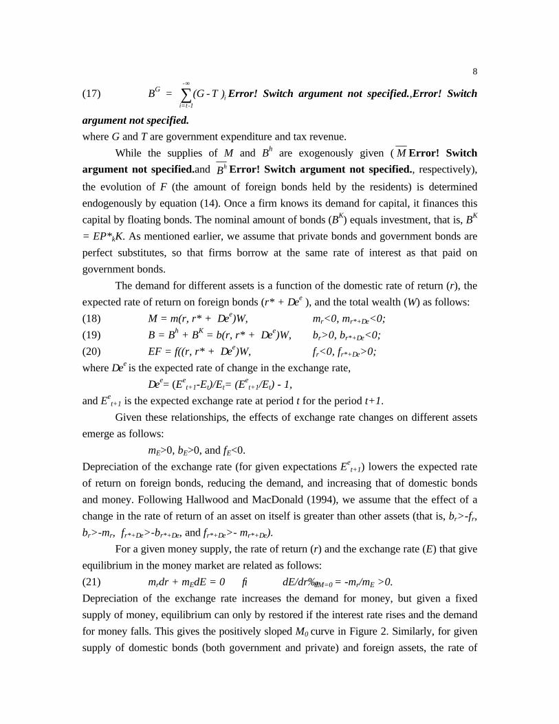
(17) BG = i=t-1

-

i(G - T )∞

∑ Error! Switch argument not specified.,Error! Switch

argument not specified.

where G and T are government expenditure and tax revenue.

While the supplies of M and Bh are exogenously given ( M Error! Switch

argument not specified.and hB Error! Switch argument not specified., respectively),

the evolution of F (the amount of foreign bonds held by the residents) is determined

endogenously by equation (14). Once a firm knows its demand for capital, it finances this

capital by floating bonds. The nominal amount of bonds (BK) equals investment, that is, BK

= EP*kK. As mentioned earlier, we assume that private bonds and government bonds are

perfect substitutes, so that firms borrow at the same rate of interest as that paid on

government bonds.

The demand for different assets is a function of the domestic rate of return (r), the

expected rate of return on foreign bonds (r* + ∆ee ), and the total wealth (W) as follows:

(18) M = m(r, r* + ∆ee)W, mr<0, mr*+∆e<0;

(19) B = Bh + BK = b(r, r* + ∆ee)W, br>0, br*+∆e<0;

(20) EF = f((r, r* + ∆ee)W, fr<0, fr*+∆e>0;

where ∆ee is the expected rate of change in the exchange rate,

∆ee= (Eet+1-Et)/Et= (Ee

t+1/Et) - 1,

and Eet+1 is the expected exchange rate at period t for the period t+1.

Given these relationships, the effects of exchange rate changes on different assets

emerge as follows:

mE>0, bE>0, and fE<0.

Depreciation of the exchange rate (for given expectations Eet+1) lowers the expected rate

of return on foreign bonds, reducing the demand, and increasing that of domestic bonds

and money. Following Hallwood and MacDonald (1994), we assume that the effect of a

change in the rate of return of an asset on itself is greater than other assets (that is, br>-fr,

br>-mr, fr*+∆e>-br*+∆e, and fr*+∆e>- mr*+∆e).

For a given money supply, the rate of return (r) and the exchange rate (E) that give

equilibrium in the money market are related as follows:

(21) mrdr + mEdE = 0 → dE/drdM=0 = -mr/mE >0.

Depreciation of the exchange rate increases the demand for money, but given a fixed

supply of money, equilibrium can only by restored if the interest rate rises and the demand

for money falls. This gives the positively sloped M0 curve in Figure 2. Similarly, for given

supply of domestic bonds (both government and private) and foreign assets, the rate of

9

return (r) and the exchange rate (E) that give equilibrium in the domestic bonds and

foreign assets market are shown by the following equations:

(22) brdr + bEdE = 0 → dE/drdB=0 = -br/bE <0; and

(23) frdr + fEdE = 0 → dE/drdF=0 = -fr/fE <0.

The B0 curve in Figure 2 is negatively sloped because an increase is the exchange rate

increases the demand for bonds, and equilibrium is restored if the demand equals the

supply of bonds by decreasing the interest rate (r). Note that dE/drdB=0 > dE/drdF=0 (as

br>-fr and fE >-bE ).

Asset market equilibrium occurs when the demands for the different assets equal

their respective supplies. There are, however, only two independent equations to

determine two independent variables that give asset market equilibrium (the wealth

constraint, equation 17, makes equilibrium in the third market redundant). Thus, the

interest rate and exchange rate that give asset market equilibrium emerge from solving the

following two implicit equations:

(24) M Error! Switch argument not specified.- m(r, r* + ∆ee)W =0, and

(25) B Error! Switch argument not specified.- b(r, r* + ∆ee)W = 0.

This is shown by the intersection of the B0 and M0 curves in Figure 2.

Exchange Rate Determination in the Short-Run and the Long-Run

Broadly speaking, the short-run exchange rate clears the asset market while the

current account balance, by changing foreign held assets (F), determines the long-run

exchange rate. The introduction of physical capital, as mentioned earlier, causes

adjustments in both the asset and goods markets. Changes in firms' investment decisions

lead to an increase/decrease of the supply of private bonds, where instantaneous

adjustments determine the short-run exchange rate and the interest rate. Investment

decisions of firms also affect the supply-side of the goods market. This effect, along with

the demand for capital goods (which is a traded good) affects the current account and

long-run equilibrium exchange rate and interest rate.

To analyze the effects of an exogenous disturbance in the economy, we distinguish

between the short-run and the long-run adjustment periods. In both periods, asset market

and current account adjustments occur. In the short-run, the initial adjustments in the

economy are analyzed, while in the long-run, the investment decisions of firms and their

effects in the economy are analyzed.

Adjustment processes after shocks to our system of equations with endogenous

capital are distinguished as follows:

10

(i) Short-Run Asset Market Adjustments: The instantaneous effects of a

disturbance in the asset market are analyzed. The changes in the demands for different

assets are examined, and the adjustment to the asset market equilibrium leading to the

determination of the short-run exchange rate and interest rate are analyzed.

(ii) Short-Run Current Account Adjustments: In this period, the effects of asset

price changes on the demand side of the goods market are studied. Specifically, the effects

of price changes on income, saving, consumption, and the current account are examined.

The end-of-the-period equilibrium exchange rate and interest rate are determined by

capital flows resulting from changes in the current account balance.

(iii) Long-Run Asset Market Adjustments: Here, the effects of monetary policy on

the private sector are considered. In this period, firms make adjustments to their capital

stocks, given the new exchange rate and interest rate. We explore the effects of these

investment decisions on the asset market and the determination of the equilibrium values

of the exchange rate and the interest rate.

(iv) Long-Run Current Account Adjustments: In this period, the effects of

investment decisions on the current account, capital flows, and the determination of the

final interest rate and exchange rate are determined. Investment decisions affect both the

supply side and the demand side of the traded goods sector and, as such, affect the current

account. The movement of the economy to the equilibrium exchange rate and interest rate

that together give current account balance is studied. Final (long-run) equilibrium is a state

where no wealth is accumulating, with no changes in net-investment, saving equals

investment, and the current account balances.

Given this set-up, an increase in the money supply by open market operations is

considered next.

3. Effects of Increases in the Money Supply by Open Market Operations

The initial equilibrium appears in Figure 2 with the B0 and M0 curves in the asset

market and Y0 and D0 in the traded goods sector. The equilibrium exchange rate and

interest rate are E0 and r0, respectively, and the current account balances. When the

central bank increases the money supply by an open market purchase of bonds,

government bonds held by the household (Bh) decrease and the money supply (M)

increases. This causes the following sequence of events in the economy, which follows our

schema enumerated in the last section.

(i) Short-Run Asset Market Adjustments: When the money supply increases by

open market operations, equilibrium in the money market is restored by either decreasing

the interest rate or increasing the exchange rate, both of which increase the demand for

11

money. Similarly, when the supply of bonds decreases, equilibrium in this market is

restored by decreasing the demand for bonds by decreasing either the interest rate or the

exchange rate.

The effects these changes have on the equilibrium exchange rate and interest rate

emerge by using the implicit function rule on equations (24)-(25) and Crammer's rule. The

results are as follows:

(26) δr/δM = [(1-m)bE + mEb]/D1<0; δE/δM = -[mrb+ br(1-m)]/D1>0;

(27) δr/δB = -[(1-b)mE + bEm]/D1>0; δE/δB = [mr(1-b)+ brm)]/D1=?;

where D1 = mrbE - brmE <0 since br > -mr, and (1-b)>m and the sign of δE/δB can be

either positive or negative.

The total effect of open market operations on the interest rate and the exchange

rate adds the effects of the increase in money supply and the decrease in the bond supply

as follows:

(28) δr/δM - δr/δB = (bE + mE )/D1<0, and

(29) δE/δM -δE/δB =-( mr+ br)/D1>0.

This is the leftward movement of M0 to M1 and B0 to B1 seen in Figure 2, with the new

equilibrium represented by the intersection of the M1 and B1 curves in Figure 2. Reduction

in the supply of domestic bonds creates an excess demand, pushing the interest rate down.

A lower interest rate, however, leads to a higher demand for foreign bonds, putting

downward pressure on the exchange rate.7 Thus, the short-run effect of an open market

operation (derived from asset market equilibrium) gives a higher (depreciated) exchange

rate (E1) and a lower interest rate (r1) than the initial values. Note that the real exchange

rate (q= EP*/PN) increases by the same proportion as that of the nominal exchange rate.

(ii) Short-Run Current Account Adjustment: Here, the effects of changes in the

exchange rate and the interest rate are studied on the demand side of the goods market.

The initial effect of a higher exchange rate is an increase in the real exchange rate that

decreases the quantity demanded of the traded consumption good. This, with a fixed

supply, improves the current account as follows:(30) dCA= - q

Tc Error! Switch argument not specified.P*T/PN dE>0,

qTc Error! Switch argument not specified.<0,

where qTc Error! Switch argument not specified. is the partial derivative of the traded

consumption good with respect to the real exchange rate. A decrease in consumption of

the traded good increases saving (see equation 13) that can either cause increased 7 Note that with no adjustment in the current account in this period, the supply of foreign bonds availabledomestically is fixed.

12

investment in physical capital or the accumulation of foreign assets. Since investment

decisions are made in the long run (discussed later), however, all increased saving during

this period leads to the accumulation of foreign assets. This manifests itself in the deficit in

the capital account (equal to the current account surplus). Thus, the current account

equals the excess of saving over the current level of investment.

The current account surplus puts downward pressure on the exchange rate and, as

such, it appreciates (i.e., E decreases). This is shown in the asset market as an increase in

foreign assets and thereby in nominal wealth, leading to the rightward movement of the M

curve (to M2) and the leftward movement of the B curve (to B2) in Figure 2. These results

are given as follows:

(31) dr/dFdM=0 = -mE/mr >0; and

(32) dr/dFdB=0 = -bE/br <0.

The end-of-the-period equilibrium exchange rate (E2) is lower than the initial short-run

level (E1).8 As foreign assets (F) accumulate, income increases (see equation 12) and

consumption of the traded consumption good increases, moving the current account

toward balance. The increase in consumption appears as the movement of the demand for

traded goods leftwards (from D0 to D1) in Figure 2. Note that in equilibrium, the economy

runs a trade-account deficit, financed by the interest earnings from foreign assets.

In the nontraded sector, a higher short-run asset market equilibrium nominal

exchange rate and a larger income increase the demand for goods produced in the sector,

increasing the price of nontraded goods. This, along with a falling nominal exchange rate

in the current-account adjustment period (from E1 to E2), decreases the real exchange

rate. Because the price of the nontraded good increases and the nominal exchange rate

decreases in this period, the decrease in the real exchange rate is proportionally more than

the nominal rate.

(iii) Long-Run Asset Market Adjustment: Given the new interest rate and exchange

rate, firms make their investment decisions. Note that these variables affect investment in

the various sectors differently. For example, while a lower interest rate increases

investment in all sectors (though with different intensities, depending on the respective

elasticities of capital demand), a higher exchange rate (E2 as compared to E0) lowers

investment in the nontraded sector only. In this sector, an increase in the exchange rate

works in the opposite direction to the decrease in the interest rate. Depending on which

8 Note that the interest rate may also change in this period. This new interest rate, however, will be lowerthan the initial rate r0, and not shown in the Figure as we are interested in exchange rate volatility.

13

effect is stronger, the nontraded sector invests/disinvests. Overall investment in the

economy depends on the relative capital intensities of the different sectors. Assuming that

investment in the traded and capital goods sectors dominates that in the nontraded sector

(if negative), the overall investment in the economy increases.

As mentioned earlier, the increase in the demand for capital goods affects both the

goods and asset markets. In the long-run asset market adjustment period, however, the

asset market equilibrium and the determination of the exchange rate and the interest rate

are explored. To invest in capital, firms float new bonds (equal to the nominal value of

investment). This increases the supply of domestic bonds, lowering their price and

increasing the interest rate. The effects of an increase in the private bond supply on the

interest rate and the exchange rate is shown by a rightward shift in the B2 curve to B3 in

Figure 3. Higher wealth increases the demand for both money holdings and foreign bonds.

The former is shown by a rightward movement of the M curve (from M2 to M3). The

change in the equilibrium exchange rate and interest rate due to increased private bond

supply is derived by using implicit function rule. The result is as follows:

(33) δr/δB = -[(1-b)mE + mbE]/D1>0, and δE/δB = [mr(1-b)+ mbr]/D1,

where D1 was defined earlier and δE/δB can be either positive or negative. Again, asset

market equilibrium determines the short-run interest rate and exchange rate. Note that

while the effect of an increase in the supply of bonds on the interest rate is positive, the

effect on the exchange rate is ambiguous. Two opposing effects act on the exchange rate.

First, increases in bond supply raise nominal wealth (W), thereby strengthening the

demand for all assets including foreign bonds. This puts downward pressure on the

exchange rate. Second, the higher interest rate decreases the demand for foreign bonds

and appreciates the currency. Depending on which of these effects dominate, the exchange

rate in the long-run asset market equilibrium may go up or down. These cases are shown

in Figures 3a and 3b, respectively.

(iv) Long-Run Current Account Adjustment: Higher capital investment affects the

current account in two ways. On the one hand, an increase in the demand for capital goods

occurs in different sectors, and this worsens the current account deficit. This appears in

Figures 3a and 3b as leftward shifts in the demand curve for traded goods (from D1 to D2).

On the other hand, more investment leads to an increase in output supplied by firms that

improves the current account. In Figures 3a and 3b, this appears as a leftward shift in the

supply curve (from Y0 to Y1). The total effect of investment on the current account, thus,

depends on these two effects as follows:

(34) dCA = (yTr + yK

r)dr- (krdr + kE dE),

14

yTr<0, yK

r<0, kE<0, kr<0, and kr > kE .

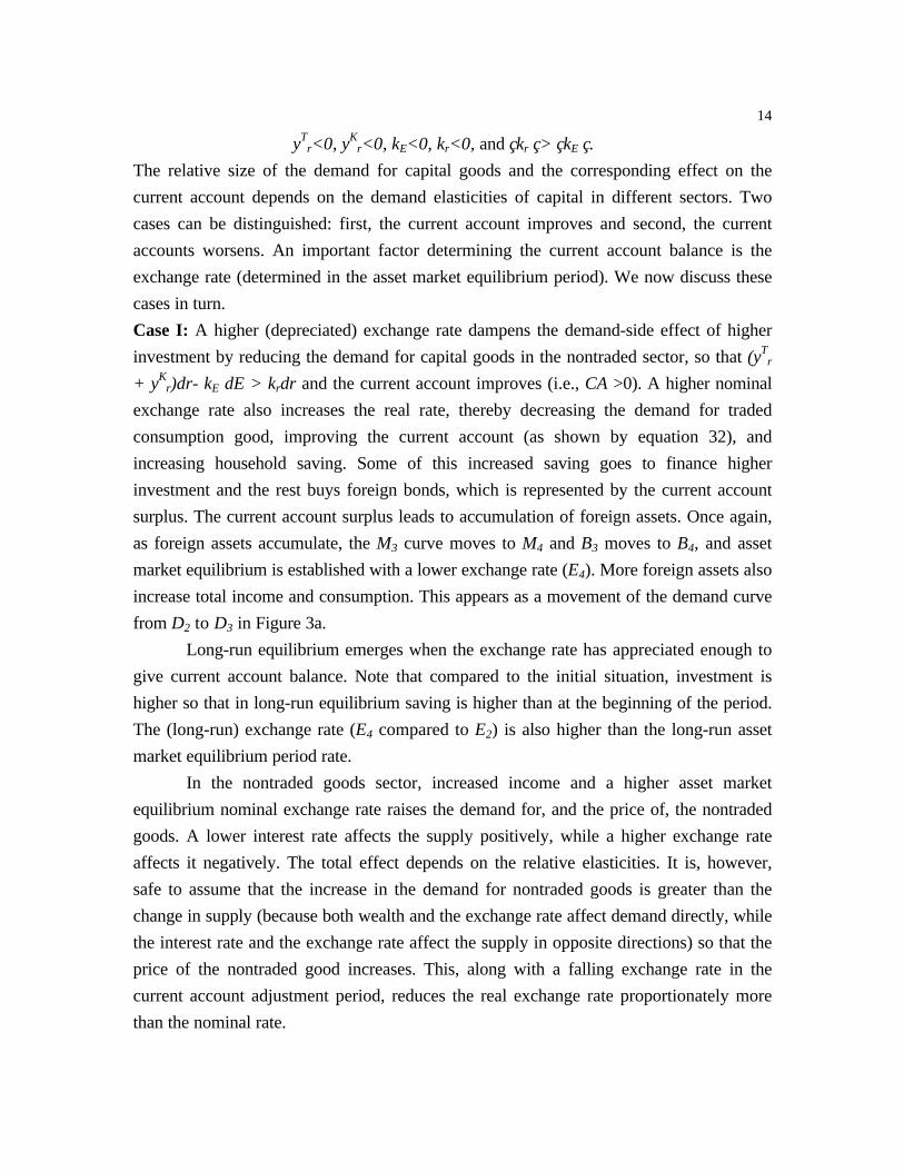
The relative size of the demand for capital goods and the corresponding effect on the

current account depends on the demand elasticities of capital in different sectors. Two

cases can be distinguished: first, the current account improves and second, the current

accounts worsens. An important factor determining the current account balance is the

exchange rate (determined in the asset market equilibrium period). We now discuss these

cases in turn.

Case I: A higher (depreciated) exchange rate dampens the demand-side effect of higher

investment by reducing the demand for capital goods in the nontraded sector, so that (yTr

+ yKr)dr- kE dE > krdr and the current account improves (i.e., CA >0). A higher nominal

exchange rate also increases the real rate, thereby decreasing the demand for traded

consumption good, improving the current account (as shown by equation 32), and

increasing household saving. Some of this increased saving goes to finance higher

investment and the rest buys foreign bonds, which is represented by the current account

surplus. The current account surplus leads to accumulation of foreign assets. Once again,

as foreign assets accumulate, the M3 curve moves to M4 and B3 moves to B4, and asset

market equilibrium is established with a lower exchange rate (E4). More foreign assets also

increase total income and consumption. This appears as a movement of the demand curve

from D2 to D3 in Figure 3a.

Long-run equilibrium emerges when the exchange rate has appreciated enough to

give current account balance. Note that compared to the initial situation, investment is

higher so that in long-run equilibrium saving is higher than at the beginning of the period.

The (long-run) exchange rate (E4 compared to E2) is also higher than the long-run asset

market equilibrium period rate.

In the nontraded goods sector, increased income and a higher asset market

equilibrium nominal exchange rate raises the demand for, and the price of, the nontraded

goods. A lower interest rate affects the supply positively, while a higher exchange rate

affects it negatively. The total effect depends on the relative elasticities. It is, however,

safe to assume that the increase in the demand for nontraded goods is greater than the

change in supply (because both wealth and the exchange rate affect demand directly, while

the interest rate and the exchange rate affect the supply in opposite directions) so that the

price of the nontraded good increases. This, along with a falling exchange rate in the

current account adjustment period, reduces the real exchange rate proportionately more

than the nominal rate.

15

Case II: An appreciated exchange rate induces effects that worsen the current account.

On the one hand, the appreciated exchange rate increases the demand for capital goods in

the nontraded sector and also increases the demand for traded consumption goods

(relative to nontraded consumption goods). A worsening current account translates into

selling foreign bonds. A fall in foreign bonds held by residents decreases nominal wealth

shifting the M curve leftwards (from M3 to M4) and the B curve rightwards (from B3 to

B4,) in Figure 3b. The worsening current account is cushioned as fewer foreign assets

dampen total income and consumption and appear as rightward movement of the D curve

(from D2 to D3).

Long-run equilibrium emerges when the exchange rate adjusts enough to give

current account balance. As long as residents hold foreign bonds, this will occur with a

trade deficit financed by foreign interest earnings. Investment is higher than initial

situation, implying (ex-post) saving to be higher. Note, however, that composition of

saving (and wealth) is different than what we had in case I. Now, foreign bonds held by

residents are lower than the initial situation.

In the nontraded-goods sector, higher output (resulting from higher investment)

and lower demand (due to lower asset market equilibrium exchange rate) lowers the price

of the traded goods. During the current account adjustment period, when the nominal

exchange rate adjusts upwards, increases the real exchange rate proportionally more than

the nominal rate.

4. Conclusion

Admittedly when endogenous physical capital enters a portfolio balance model, the

model becomes more complicated, but, as we have shown, it does remain tractable and

plausible results were derived. Nor is the insertion of endogenous physical capital an idle

exercise. This is because extant portfolio balance models, which many international

economists would regard as being on the cutting edge of analytical exchange rate

modeling, ignore the interplay that may well exist between changes in private sector

investment and the equilibrium exchange rate. This would not matter except that extant

portfolio balance exchange rate models are known to have a poor track record, even

'within sample', of tracking the exchange rate over time. Thus, at the very least, this paper

should be regarded as an exercise in persuasion -- encouraging exchange rate

econometricians to include proxies for domestic investment in their estimating equations.

We have developed a portfolio balance model where capital is considered both as

an asset and as a good produced and demanded by firms. The effects of a monetary

disturbance were then examined. Consideration of capital leads to adjustments in the

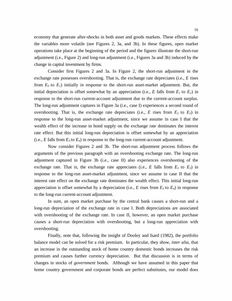
16

economy that generate after-shocks in both asset and goods markets. These effects make

the variables more volatile (see Figures 2, 3a, and 3b). In these figures, open market

operations take place at the beginning of the period and the figures illustrate the short-run

adjustment (i.e., Figure 2) and long-run adjustment (i.e., Figures 3a and 3b) induced by the

change in capital investment by firms.

Consider first Figures 2 and 3a. In Figure 2, the short-run adjustment in the

exchange rate possesses overshooting. That is, the exchange rate depreciates (i.e., E rises

from E0 to E1) initially in response to the short-run asset-market adjustment. But, the

initial depreciation is offset somewhat by an appreciation (i.e., E falls from E1 to E2) in

response to the short-run current-account adjustment due to the current-account surplus.

The long-run adjustment captures in Figure 3a (i.e., case I) experiences a second round of

overshooting. That is, the exchange rate depreciates (i.e., E rises from E2 to E3) in

response to the long-run asset-market adjustment, since we assume in case I that the

wealth effect of the increase in bond supply on the exchange rate dominates the interest

rate effect. But this initial long-run depreciation is offset somewhat by an appreciation

(i.e., E falls from E3 to E4) in response to the long-run current-account adjustment.

Now consider Figures 2 and 3b. The short-run adjustment process follows the

arguments of the previous paragraph with an overshooting exchange rate. The long-run

adjustment captured in Figure 3b (i.e., case II) also experiences overshooting of the

exchange rate. That is, the exchange rate appreciates (i.e., E falls from E2 to E3) in

response to the long-run asset-market adjustment, since we assume in case II that the

interest rate effect on the exchange rate dominates the wealth effect. This initial long-run

appreciation is offset somewhat by a depreciation (i.e., E rises from E3 to E4) in response

to the long-run current-account adjustment.

In sum, an open market purchase by the central bank causes a short-run and a

long-run depreciation of the exchange rate in case I. Both depreciations are associated

with overshooting of the exchange rate. In case II, however, an open market purchase

causes a short-run depreciation with overshooting, but a long-run appreciation with

overshooting.

Finally, note that, following the insight of Dooley and Isard (1982), the portfolio

balance model can be solved for a risk premium. In particular, they show, inter alia, that

an increase in the outstanding stock of home country domestic bonds increases the risk

premium and causes further currency depreciation. But that discussion is in terms of

changes in stocks of government bonds. Although we have assumed in this paper that

home country government and corporate bonds are perfect substitutes, our model does

17

suggest that attention should be paid to corporate bonds (and, for that matter, other

private sector securities including stocks and shares). Thus, we have shown that following

a monetary expansion and consequent currency depreciation, profitability in the traded

goods sector increases. We expect, ceteris paribus, that the latter will tend to reduce any

risk premium on home country corporate securities and, therefore, to strengthen -- relative

to what it would have been -- the domestic currency on the foreign exchanges.

Furthermore, we think that emphasizing the role of private-sector profitability in the

exchange rate adjustment process is in keeping with the recent phenomenon of

international portfolio diversification across other countries' corporate securities.

References

Allen, P. R. and P. B. Kenen (1976), “Portfolio Adjustment in Open Economies: AComparison of Alternative Specifications,” Welfwirtschaftliches Archiv, (Reviewof World Economics), 112 (1), 33-72.

Allen, P. R. and P. B. Kenen (1978), The Balance of Payments, Exchange Rates andEconomic Policy (A Survey and Synthesis of Recent Developments), Centre ofPlanning and Economic Research, Athens.

Branson, W. H. (1977), “Asset Markets and Relative Prices in Exchange RateDetermination,” Sozial Wissenchaftliche Annalen, Band 1.

Branson, W. H. and D. W. Henderson (1985), “The Specification and Influence of AssetMarkets,” in R. W. Jones and P. B. Kenen (eds.) Handbook of InternationalEconomics, Volume II, North Holland, Amsterdam.

Connolly, Michael and Dean Taylor (1976), “Devaluation, Traded Goods andInternational Assets,” in E. Classen and P. Salin (eds.) Recent Issues inInternational Monetary Economics, North Holland Publishing Company,Amsterdam.

Dar, Atul A. and Saleh Amirkhalkhali (1991), “The Behaviour of the Current AccountBalance: An Empirical Study of OECD Countries,” Economic Notes, 20 (3), 561-70.

Dooley, M. P. and P. Isard (1982), “A Portfolio Balance Rational Expectations Model ofthe Dollar-Mark Exchange rate,” Journal of International Economics 12, 257-76.

Dornbusch, Rudiger (1975), Open Economy Macroeconomics, Basic Books, Inc.Publishers, New York.

18

Dornbusch, Rudiger and Stanley Fischer (1980), “Exchange Rates and the CurrentAccount,” American Economic Review, 70 (5), 960-971.

Franlel, J. A. (1983), “Monetary and Portfolio Balance Models of Exchange RateDetermination,” In J. Bhandari and B. Putnam (eds.) Economic Interdependenceand Flexible Exchange Rates, Cambridge, MIT Press.

Frankel, J. A. (1979), “On the Mark: A Theory of Floating Exchange Rates Based on RealInterest Rate Differences,” American Economic Review 69, 610-22.

Frenkel, Jacob A. and Carlos A. Rodriguez (1975), “Portfolio Equilibrium and the Balanceof Payments: A Monetary Approach,” American Economic Review, 65 (4), 674-688.

Genberg, H. and H. Kierzkowski (1979), “Impact and Long run Effects of economicDisturbances in a Dynamic Model of Exchange Rate Determination,”Welfwirtschaftliches Archiv, (Review of World Economics), 116 (1), 605-27.

Hallwood, Paul and Ronald MacDonald (1994), International Money and Finance,Second edition, Basil Blackwell, Oxford.

Hooper, P and J. Morton (1983), “Fluctuations in the Dollar: A Model of Nominal andReal Exchange Rate Determination,” Journal of International Money and Finance1, 39-56.

Isard, P. (1978), Exchange Rate Determination: A Survey of Popular Views and RecentModels, Princeton Studies in International Finance, No. 42.

Kouri, Pentti, J. K. (1976), “The Exchange Rate and the Balance of Payments in the Shortrun and the Long run: A Monetary Approach,” The Scandanavian Journal ofEconomics, 78 (2), 280-304.

Kouri, Pentti, J. K. (1978), Balance of Payments and the Foreign Exchange Market: ADynamic Partial Equilibrium Model, NBER Working Paper, No. 644, NBER,Cambridge, MA.

Krueger, Anne O. (1983), Exchange Rate Determination, Cambridge University Press,New York.

Meese, R. A. and K. Rogoff (1983), “Empirical Exchange Rate Models of the Seventies:Do They Fit Out of Sample?” Journal of International Economics 14, 3-24.

19

Rodriguez, Carlos A. (1980), “The Role of Trade Flows in Exchange Rate Determination:A Rational Expectations Approach,” Journal of Political Economy, 80 (6), 1148-58.

Ruffin, Roy J. (1979), “Growth and the Long run Theory of International CapitalMovement,” American Economic Review, 69 (5), 832-42.

Sachs, Jeffrey D. (1981), “The Current Account and Macroeconomic Adjustment in the1970s,” Brookings Papers on Economic Activity, 1, 201-268.

Sachs, Jeffrey D. (1983), “Aspects of Current Account Behavior of OECD Economies,”in E. Claasen and P. Salin (Eds.), Recent Issues in the Theory of Exchange Rates,1, North Holland, Amsterdam & New York.

Serven, Luis (1995), “Capital Goods Imports, the Real Exchange Rate and the CurrentAccount,” Journal of International Economics, 39, 79-101.

Witte, James G. (1963), “The Microfoundations of the Social Investment Function,”Journal of Political Economy, 71 (3), 441-56.

20

Figure 1: Demand and Supply of Capital

EPk*

I(r1)

I(r0)

Y0k Y1

k Yk

21

Figure 2: Short-run Adjustments

E M1

M2 M0

D1

D0

E1

E2

E0

B2 B1 B0

Y Y0 r1 r0 r

22

Figure 3a: Long-run Adjustments: Exchange Rate Depreciation in the Asset Market Equilibrium and Improvement in the Current Account

E D3

B4 B3

D2 B2 M2 M3

M4

D1

E3

E4

E2

Y Y1 Y0 r1 r2 r

23

Figure 3b: Long-run Adjustments: Exchange Rate Appreciation in the Asset-Market Equilibrium and Worsening of the Current-Account

D2 E B2 B3 B4

D3

D1 M2

M4

M3

E2

E4

E3

Y Y1 Y0 r1 r2 r