density variations during solidification of lamellar graphite iron1156419/fulltext01.pdf · 2017....

LICENTIATE THESIS

Density variations during solidification of lamellar graphite iron

Kristina Hellström

Department of Materials and Manufacturing

SCHOOL OF ENGINEERING, JÖNKÖPING UNIVERSITY

Jönköping, Sweden 2017

Licentiate Thesis in Materials and Manufacturing

Density variations during solidification of lamellar graphite iron Kristina Hellström Department of Materials and Manufacturing School of Engineering, Jönköping University SE-551 11 Jönköping, Sweden [email protected] Copyright © Kristina Hellström Research Series from the School of Engineering, Jönköping University Department of Materials and Manufacturing Dissertation Series No. 32, 2017 ISBN: 978-91-87289-33-00 Published and Distributed by School of Engineering, Jönköping University Department of Materials and Manufacturing SE-551 11 Jönköping, Sweden Printed in Sweden by BrandFactory AB Kållered, 2017

mailto:[email protected]


i

ABSTRACT With increasing legislative demands on the reduction of emissions from combustion engines, manufacturers of heavy vehicles are looking to increase the pressure during the combustion process. This will put higher demands on the material used in engine applications and the importance of sound components increases. One factor that has to be gained control over is the formation of shrinkage porosity, which in lamellar graphite iron is forming a network of voids, thereby reducing the mechanical properties.

The mechanisms behind shrinkage porosity formation are many and complex. However, one factor of great importance is the volume and density changes that the material goes through during solidification. Browsing through literature, few data could be found regarding density measurements of liquid cast iron. This has to do with the difficulties of measuring the property in question correctly. Although many methods have been employed for measurements of liquid metals and alloys, none of them measure the density directly, calculations are always required.

In order to reduce the occurrence of defects in castings of complex geometry, the industry relies heavily on different simulation software. For casting simulation, these mathematical models are most often based on the laws of heat transfer. These laws consist of heat balances and, within them, relations between the so called thermophysical properties, of which density is one.

The aim of the work at hand has been to establish a picture of the field – the existing body of data and measurement methods has been mapped – and to investigate the volume and density changes displayed by grey cast iron during solidification. Experimental investigations of lamellar graphite iron of varying carbon content have been performed in the liquid state. Measurements have also been performed in the solid state, in the austenitic range, then on low-carbon steels. The results from these investigations have then been used for modelling and simulation of volume change, with MATLAB as calculation tool. The model has been based on the finite volume method, FVM (also known as control volume finite difference method, CV-FDM) with both cylindrical and spherical polar co-ordinates. Modelling of the influence of the graphite fraction in the austenitic range has also been initiated.

Keywords: density, grey cast iron, measurements, modelling


iii

SAMMANFATTNING Lagstiftning med krav på minskade avgasutsläpp från förbränningsmotorer gör att tillverkare önskar öka förbränningstrycket i motorn. Detta medför en ökad påkänning på materialet i motorkomponenterna och betydelsen av defektfritt gjutgods ökar. En defekt som är särskilt intressant i sammanhanget är krympporer, som i lamellärt gjutjärn bildar ett nätverk av hålrum, något som påverkar hållfasthetsegenskaperna negativt.

Mekanismerna för bildning av krympporer är flera och komplexa. En faktor av avgörande betydelse är dock de volym- och densitetsförändringar som materialet genomgår vid stelning. Vid en litteraturgenomgång konstaterades att få mätdata kunde hittas för gjutjärns densitet i smält tillstånd. Detta har att göra med svårigheterna att mäta just denna materialegenskap korrekt. Även om flera olika mätmetoder har tillämpats på flytande metaller och legeringar mäter ingen metod densiteten direkt, beräkningar måste alltid göras.

För att minska defektförekomsten i gjutgods med komplex geometri, förlitar sig industrin i hög grad på olika simuleringsprogram. När det gäller gjutsimulering är dessa program baserade på värmeöverföringslagarna, vilka består av energibalanser och samband mellan termofysikaliska egenskaper, såsom bl.a. densitet.

Målet med föreliggande undersökning har varit att bilda sig en uppfattning om hur mycket och vilka densitetsdata som finns i litteraturen, samt att experimentellt undersöka de volym- och densitetsförändringar gråjärn genomgår vid stelning. När det gäller undersökningarna av de olika legeringarna i flytande tillstånd har dessa genomförts på lamellärt gjutjärn med flera olika kolhalter. Mätningar har också genomförts i austenitområdet, då på lågkolhaltiga stål. Resultaten från undersökningarna har sedan använts för modellering och simulering av volymförändring, som sedan jämförts med utförda mätningar. Modelleringen har gjorts i MATLAB med finita volymmetoden (även känd som finita differensmetoden med kontrollvolym) med både cylindriska och sfäriska polära koordinater. Modellering av grafitfraktionens inverkan vid volymförändringar under austenitfasen har inletts.

Nyckelord: densitet, gjutjärn, mätning, simulering


v

ACKNOWLEDGEMENTS I would like to express my sincere gratitude to:

My main supervisor, Professor Attila Diószegi, first and foremost, for giving me the opportunity to return to the field of metallurgy and for giving me the guidance and the freedom I have needed to reach this point. My supervisor Dr Lucian Diaconu for displaying a true interest in my work, for giving valuable comments and for the hours in the foundry. Peter Gunnarsson, for machining many of the tiny dilatometer samples by hand. Taishi Matsushita, for issues regarding dilatometer measurements and Thermo-calc. Jacob Steggo and Toni Bogdanoff, for matters regarding the measurement equipment. Jörgen Bloom, for teaching me the SEM. Åsa Hansen, for preparing different etchants and Esbjörn Ollas and Lars Johansson, for providing excellent service in the workshop. All the members of the SPOFIC I & II projects, for enjoyable project meetings, and especially project leader Dr Jessica Elfsberg, for creating such a nice work atmosphere. The funding agency VINNOVA, for financial support. Colleagues and friends at Jönköping University, especially at the Department of Materials and Manufacturing, for making it a pleasure to go to work. Rev. Hans Boeryd, for the encouragement to take up these studies in the first place and for the support during the course of this work. Finally, I would like to thank my relatives and friends for inviting me to dinner now and then, with interesting (and long) discussions. I am very grateful to my cousin Kerstin and her family, for all the support, patience and good times.

Kristina Hellström Jönköping, August 2017


vii

SUPPLEMENTS The following supplements constitute the basis of this thesis:

Supplement I K. Hellström, A. Diószegi, and L. Diaconu; A Broad Literature Review of Density Measurements of Liquid Cast Iron.

Published in Metals, 2017, 7(5), 165.

K. Hellström was the main author. A. Diószegi provided the idea for the paper and reviewed it. L. Diaconu contributed the diagrams and reviewed the paper.

Supplement II K. Hellström, L. Diaconu and A. Diószegi; Density and thermal expansion coefficients of liquid grey cast iron and austenite.

Manuscript submitted to Metallurgical and Materials Transactions A.

K. Hellström was the main author. A. Diószegi provided the idea and guided the work. L. Diaconu planned and performed the casting of the alloys, assisted by K. Hellström. L. Diaconu also contributed with Thermo-calc calculations, diagrams and reviewing of the paper.

Supplement III K. Hellström, P. Svidró, L. Diaconu and A. Diószegi; Density variations during solidification of grey cast iron.

Presented at the International Symposium on the Science and Processing of Cast Iron (SPCI-XI), 4-7 September 2017 in Jönköping, Sweden

K. Hellström was the main author. Measurement data was provided by K. Hellström and P. Svidró. Modelling was performed by A. Diószegi and K. Hellström. A. Diószegi and L. Diaconu reviewed the paper. L. Diaconu prepared the graphs.

viii

Additional work:

Other relevant publications not included in the thesis.

T. Andriollo, K. Hellström, M. Rostgaard Sonne, J. Thorborg, N. Tiedje and J. Hattel: Uncovering the local inelastic interactions during manufacture of ductile cast iron: How the substructure of the graphite particles can induce residual stress concentrations in the matrix. Accepted for publication in Journal of the Mechanics and Physics of Solids.


ix

TABLE OF CONTENTS

CHAPTER 1 INTRODUCTION .............................................................................................................................. 1 1.1 BACKGROUND ................................................................................................................................................................................... 1 1.2 CAST IRON ........................................................................................................................................................................................... 2 1.3 SOLIDIFICATION .............................................................................................................................................................................. 3 1.4 WHAT IS DENSITY AND WHY MEASURE IT? ..................................................................................................................... 5 1.5 DENSITY MEASUREMENT METHODS ................................................................................................................................... 6 1.6 THERMAL EXPANSION COEFFICIENT ................................................................................................................................ 11 1.7 THE EFFECT OF ALLOYING ELEMENTS ON DENSITY ................................................................................................ 11 1.8 CALCULATION METHODS ........................................................................................................................................................ 15

CHAPTER 2 RESEARCH APPROACH .............................................................................................................. 21 2.1 PURPOSE AND AIM ...................................................................................................................................................................... 21 2.2 RESEARCH DESIGN ...................................................................................................................................................................... 21 2.3 MATERIAL AND EXPERIMENTAL PROCEDURE ............................................................................................................ 22 2.4 CALCULATIONS ............................................................................................................................................................................. 25

CHAPTER 3 SUMMARY OF RESULTS AND DISCUSSION ......................................................................... 31 3.1 DENSITY ............................................................................................................................................................................................ 31 3.2 THERMAL EXPANSION COEFFICIENT ................................................................................................................................ 38 3.3 MATERIAL CHARACTERISATION ......................................................................................................................................... 40 3.4 MODELLING BASED ON THE RESULTS (SUPPLEMENT III) .................................................................................... 40 3.5 FURTHER OBSERVATIONS ...................................................................................................................................................... 43

CHAPTER 4 CONCLUDING DISCUSSION ....................................................................................................... 45

CHAPTER 5 CONCLUSIONS ............................................................................................................................... 49

CHAPTER 6 FUTURE WORK ............................................................................................................................. 51

REFERENCES...........................................................................................................................................................53

APPENDED PAPERS ............................................................................................................................................... 57


xi

NOMENCLATURE

A Area of the surface [m2]

cp Specific heat [J/(kgK)]

𝐷𝐷𝐼𝐼𝐼𝐼𝐻𝐻𝐻𝐻𝐻𝐻 Hydraulic diameter [m]

d and Δd Diameter and change in diameter [m]

fs Fraction solid f γ and f gr Fraction austenite and fraction graphite

k Thermal conductivity [W/(mK)] L Total solidification heat [J/kg]

l and Δl Length and change in length [m] l0 and d0 Initial length and diameter [m]

𝑀𝑀𝑖𝑖−1→𝑖𝑖 and 𝑀𝑀𝑖𝑖→𝑖𝑖+1 Heat resistances between node i-1 and i and between i and i+1

m Mass [kg] ma Mass [kg] (weighed in air)

P Pressure [Pa]

�̇�𝑄 Change of heat content per unit time [W]

�̇�𝑄𝑔𝑔𝑔𝑔𝑔𝑔 Volumetric heat generation [W/m3]

𝑄𝑄𝑟𝑟𝑔𝑔𝑟𝑟𝑟𝑟𝑟𝑟𝑔𝑔𝐻𝐻′′′ Heat released [J/m3] q Diffusive heat flow (heat flux) perpendicular to the surface of

the area [W] r Radius [m]

Sγ Envelope of the primary dendrite T and ΔT Temperature and temperature difference [K] or [°C]

t and Δt Time and time difference [s] V Volume [m3]

x Descriptive space parameter perpendicular to the surface [m] Λ Temperature dependence of liquid density [kg/m3K]

ρ Density [kg/m3] ργ and ρgr Density of austenite and density of graphite [kg/m3]

∇2𝑇𝑇 Laplace operator [°C/m2]


1

CHAPTER 1

INTRODUCTION

CHAPTER INTRODUCTION

Why is knowledge about density variations important? Having used cast iron for such a long time, do we not know everything there is to know about the material? In this chapter, the background and context of the current work is presented. Furthermore, an introduction to measurement methods, solidification and numerical modelling is given, to facilitate further reading.

1.1 BACKGROUND

As part of moving towards a more sustainable society, producers of heavy vehicles are facing stricter regulations regarding emissions from combustion engines. In order to respond to these demands the industry has looked to augmentation of the pressure during the combustion process. This means that higher strain will be put on the material of the engine components. It is therefore ever so important that the material is sound and free from defects.

Even though cast iron has a long history, production has been dated back to 800-700 B.C. (in China) [1], it is still not understood in all details. One issue in particular, known to every person involved in foundry practice, is porosity. These can be of different sorts: gas porosity and shrinkage porosity. The former is developed when gas is precipitated to form “bubbles” in the cast products. The trait of gas porosities is that the surface of the cavity is smooth and lacks protuberances. Shrinkage porosity, on the other hand, has dendrites protruding the cavity surface. The formation mechanisms behind shrinkage porosity are not fully understood, but it has been suggested that solidification shrinkage and gas precipitation cooperate.[2]

Shrinkage porosity in cast components is detrimental to the mechanical properties of the material. It may also, in some varieties of cast iron, form a network of voids in the casting, a network that could act as a gateway between the channels for fuel and cooling agent. Defects of this type may reveal themselves only after machining, hereby making the component a quite costly piece of scrap.

To maintain a sustainable production, resources must be used in an efficient way. Scrapping in too high amounts must therefore be avoided. This is beneficial not only from an environmental perspective but also from an economical viewpoint. To achieve sustainable production, prediction of casting outcome is an important tool. Various simulation software is available on the market, however, the result in terms of outcome will only be as good as the database and the model will allow.

2

1.2 Cast iron

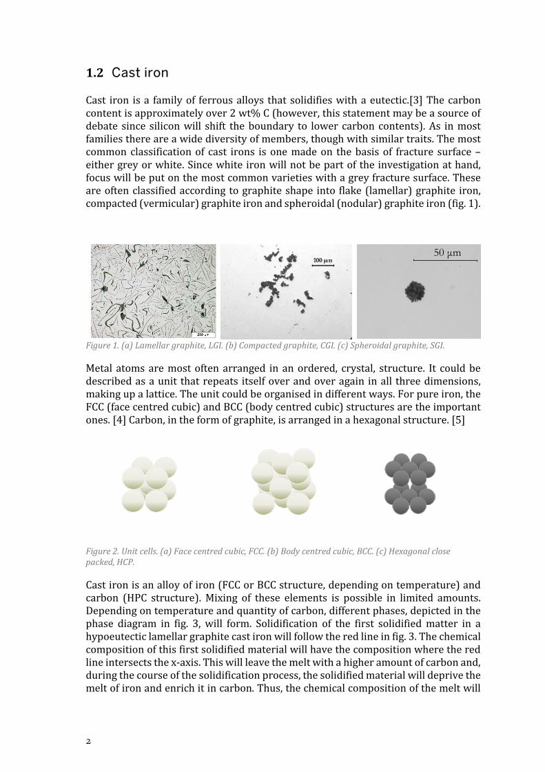
Cast iron is a family of ferrous alloys that solidifies with a eutectic.[3] The carbon content is approximately over 2 wt% C (however, this statement may be a source of debate since silicon will shift the boundary to lower carbon contents). As in most families there are a wide diversity of members, though with similar traits. The most common classification of cast irons is one made on the basis of fracture surface – either grey or white. Since white iron will not be part of the investigation at hand, focus will be put on the most common varieties with a grey fracture surface. These are often classified according to graphite shape into flake (lamellar) graphite iron, compacted (vermicular) graphite iron and spheroidal (nodular) graphite iron (fig. 1).

Figure 1. (a) Lamellar graphite, LGI. (b) Compacted graphite, CGI. (c) Spheroidal graphite, SGI.

Metal atoms are most often arranged in an ordered, crystal, structure. It could be described as a unit that repeats itself over and over again in all three dimensions, making up a lattice. The unit could be organised in different ways. For pure iron, the FCC (face centred cubic) and BCC (body centred cubic) structures are the important ones. [4] Carbon, in the form of graphite, is arranged in a hexagonal structure. [5]

Figure 2. Unit cells. (a) Face centred cubic, FCC. (b) Body centred cubic, BCC. (c) Hexagonal close packed, HCP.

Cast iron is an alloy of iron (FCC or BCC structure, depending on temperature) and carbon (HPC structure). Mixing of these elements is possible in limited amounts. Depending on temperature and quantity of carbon, different phases, depicted in the phase diagram in fig. 3, will form. Solidification of the first solidified matter in a hypoeutectic lamellar graphite cast iron will follow the red line in fig. 3. The chemical composition of this first solidified material will have the composition where the red line intersects the x-axis. This will leave the melt with a higher amount of carbon and, during the course of the solidification process, the solidified material will deprive the melt of iron and enrich it in carbon. Thus, the chemical composition of the melt will

50 μm


3

be moved to the right on the x-axis, until the eutectic point is reached. From then on, a joint growth of carbon, precipitated as graphite, will form a eutectic structure with iron, in this case with an FCC lattice - commonly known as austenite. The process of dividing the melt in this manner is known as segregation.

Figure 3. The iron-carbon phase diagram, generated in Thermo-calc. Initial solidification of an alloy with the composition 3 wt% C and 97 wt% Fe. The first solidified particles will have the chemical composition where the arrow intersects the x-axis. The next layer, at a slightly lower temperature, will have a composition slightly to the right of the first series of arrows. This will continue until the eutectic point is reached, when a joint growth of graphite and austenite will occur.

Cast iron is rarely just an alloy of iron and carbon, other elements are present to a varying degree. These elements have their own segregation patterns - they will either enrich in the melt or form a constituent of the solidifying phase. However, some elements, like magnesium, have been seen to distribute themselves rather uniformly across the metal matrix. [6]

1.3 Solidification

Solidification of cast iron, as well as most materials, will start because of the differences in heat (energy contents) between the melt and the surroundings, i.e. the mould. With a decrease in heat, the constituents of the melt must find a way to order themselves in a manner that is the most advantageous from an energy point of view.

(γ)

Austenite

Liquid

Solid (FCC)

Solid (BCC)

Eutectic point

L + S

4

The atoms which have previously been disarranged are now forming an ordered, crystal structure. [7]

The energy transport that occurs during solidification are well described in the literature on thermodynamics. The equations that describe this mechanism consists of relations between thermophysical properties, of which density is one of the more fundamental. It is also these equations that constitute the foundation for many simulation software products.

Solidification of hypoeutectic grey cast irons generally starts with nucleation and growth of austenite dendrites, hereby causing a more rapid increase in density than that of the cooling melt. This increase is soon followed by a decrease when the lower density graphite precipitates [8]. In hypereutectic grey iron the increase of melt density with temperature has been seen to slow down when the temperature has reached below the liquidus temperature, indicating the precipitation of primary graphite [9].

Investigations of solidification of cast iron by the means of DAAS (Direct Austempering After Solidification) treatment could reveal the austenite grains in samples cooled to room temperature. The grain size turned out to be rather large and each grain hosted several eutectic cells. Austenite dendrites would thus seem to provide a good number of seeds for the eutectic austenite to grow on. [10] Since the austenite of the eutectic cells share the same crystallographic orientation as the dendritic network making up the grain, it is hard to believe that the eutectic cells have been formed independently in the melt and then adhered to the dendritic network. In a later work [11] the idea that both hypo-and hyper-eutectic grey iron start to solidify by growing austenite dendrites was further developed and it was inferred that cast irons of widespread CE values, and of all graphite morphologies, solidify in a similar way – i.e. that “solidification begins with the nucleation and growth of austenite dendrites”[11] (p.49). A dissimilarity, however, was that the CGI specimen in the study showed a much finer grain structure than the lamellar and nodular irons.

From the information given above it is also clear that consensus is not established when it comes to the solidification of cast irons.

Transformation of phases are governed by the change in free energy. [7] For a unit volume of a substance, the Heimholtz free energy can be expressed comprising internal energy, pressure, volume temperature and entropy. The entropy is a measure of the amount of disorder in a system, in a crystal structure the entropy is low and in a gas the entropy is high. [12] Disorder in the solid, crystal, state comes from the thermal vibrations of the atoms at the lattice points. [7] In the liquid state disorder also results from structural disorder.

The thermal energy at higher temperatures will increase the occurrence of vacancies in the lattice structure until the long-range order of the crystalline lattice is dispersed and replaced by a short-range order. [7] Hence, the liquid has not the fully ordered structure of the solid state but it is not as chaotic as the gaseous state. This change from ordered, crystal, structure to less ordered structure will in most materials entail an increase in volume. Likewise, the arrangement of atoms into a crystal structure at solidification will in most cases mean a decrease in volume. Looking closer at the


5

formation of disordered systems into ordered ones, the bonds to the nearest neighbour must be investigated. In solids, these bonds will point in specific directions but in liquids it is equally probable that the nearest neighbour would be found in any direction. [13] Structures of liquids are therefore represented by distribution functions that will give the probability of the existence of a given number of atoms at certain positions. Investigations of undercooled metallic melts have shown that an icosahedral structure is present in these melts, more pronounced the lower the temperature. [14] This structure could also be found in melts above the liquidus temperature. There are observations of the icosahedral structure both in melts forming fcc and bcc structures in the solid state.

1.4 What is density and why measure it?

Density is defined as mass per unit volume and is written as:

𝜌𝜌 =𝑚𝑚𝑉𝑉

. (1)

The SI-unit for density is [kg/m3], but [g/cm3] is also a common way of expressing the value.

Density is generally referred to as a thermophysical property, i.e. the value is temperature dependent. As can be seen from the above equation (eq. 1) it is a measure of how much mass is concentrated in a unit volume. Irrespective of size and mass of an object, density stays the same for any pure substance, at constant temperature and pressure. [15]

At the solidification of castings, the density will vary throughout the whole process and it is of essence to have a thorough knowledge of these variations since density is one of the more fundamental thermophysical properties. The temperature dependence of the density in the liquid state, Λ, at constant pressure [16], can be written as:

Λ = �𝜕𝜕𝜕𝜕𝜕𝜕𝜕𝜕�𝐼𝐼

. (2)

With the increasing use of simulation software to predict casting outcomes it has become even more important to base the calculations on reliable data, to obtain consistent results. The accuracy of these data determines the accuracy of the whole simulation [17, 18]. As density is also a parameter at the measurements of e.g. surface tension, viscosity and thermal conductivity, bad accuracy will affect these parameters as well [19]. A thorough knowledge of density variations will enable simulation of heat conduction, solidification, elastic-plastic deformation and fluid flow, which in turn will improve product quality [20].

Accurate values of thermophysical properties are thus beneficial both for the industry (as a means for the solution of problems arising at casting of complex components) and as input data for mathematical modelling. In the latter application it has proven a valuable means in the enhancement of process control and product quality [21].

6

One of the more detrimental defects in cast iron is shrinkage cavity or shrinkage porosity. The formation of these are closely linked to the volume and density changes the material goes through during solidification. [9] It is generally known that SGI and CGI are more prone to this kind of defect than LGI is. The propensity for micro shrinkage in cast iron has been believed to be related to the amount of graphite expansion during solidification [8].

Also the structure (e.g. bond lengths, coordination numbers and bond angles) of liquids and solids has some influence on the value of the thermophysical properties. [21] The effect on density values of crystalline metals is, however, regarded to be small. (For slags and glasses, on the other hand, the structural effects are much larger.)

There are a number of different methods for density measurement of liquid and solid metals and alloys. A method can be based on the measurement of either buoyancy, hydrostatic pressure, volume or shape [22]. Some of the more frequent techniques will be reviewed below. They all have their advantages and disadvantages, and the context will decide which one will be the more suiting. One of the things all methods have in common is that the density must be calculated, by one or several operations, from data obtained in a direct or an indirect way.

1.5 Density measurement methods

As mentioned above, there are many different methods for measuring density of both pure metals and of alloys. These techniques can be based on e.g. buoyancy, hydrostatic pressure, volume or shape. There are also methods that use radiation or electric current to measure density. The most common ones are described and compared in the following paragraphs.

Archimedean method (buoyancy)

Perhaps the oldest and most well-known method of measuring density is through the use of the Archimedean principle, which says that a fluid is exerting an upward force on a body immersed in it, and that that force is equal to the weight of the displaced liquid[23]. The method is thus based on buoyancy [22] and measurements can be made either on the immersed body – then the density of the liquid has to be known, or on the liquid - with a body of known density. In the case of liquid metals a setup with a sinker and a counter weight suspended from an analytical balance has been used. In order to obtain reliable results from this kind of measurements a number of corrections must be made. [24] In the case of measurements of a liquid, the expansion of the sinker must be known and taken into account, as well as the thread suspending the sinker. Also the surface tension must be known, as well as the contact angle. [25] An advantage is that the method can be used continuously during changing temperature. [26]

Pycnometric method (volume)

The pycnometric method involves a vessel of known volume, which is completely filled with liquid metal and then left to solidify. The sample is then weighed and the


7

density can be calculated at the temperature when the vessel was filled. [9] The method is considered accurate if the volume of the vessel is truly known [27]. It is therefore preferable that the vessel material has a low coefficient of thermal expansion. The drawback of the method is that it does not allow for continuous monitoring of the expansion and contraction behaviour of the metal with temperature.

Maximum bubble pressure method (hydrostatic pressure)

Like the pycnometric method the maximum bubble pressure method allows measurements at one temperature at a time. It is based on the measurement of the pressure required to form a bubble of an inert gas at the end of a capillary immersed in the liquid metal. [26] The measurements are performed at two different levels, or depths, in the liquid and from the difference in pressure required to form a bubble at these two levels, the density can be calculated [27]. One or two capillaries can be used, in the case of one capillary, a reposition must be performed. Corrections must then be made to account for the change in liquid surface level [26].

The method is not regarded as accurate as the pycnometric method [27], however, it has the advantage over the Archimedean method in that the surface tension of the liquid does not have to be known, as long as the contact angle does not change [26]. Nor does the thermal expansion of the crucible has to be considered. It is, however, important that the temperature is kept stable during the entire two-level measurements.

The method generally requires high precision in the positioning of the capillary tip and the thermal expansion of the capillary must also be taken into account [26]. Improvements of the capillary tip (curved walls) have been made in some experiments [28] to avoid the problem of bubbles leaving the tip before they are mature.

Sessile drop (shape)

The sessile drop method employs a cylindrical sample, of known mass and volume, which is melted to form a drop on a flat surface or substrate. The drop must form symmetrically, which is most likely if the initial sample is a cylinder with sharp edges [27]. However, cylindrical samples with a conical top and chamfered at the bottom have also been used [20]. The shape of the drop, recorded by e.g. x-ray pictures or CCD camera, is then used to calculate the volume of the drop. The method allows for continuously monitoring of the drop during a temperature interval. The shape of the drop is often measured from different angles, e.g. by rotating the sample [20]. The sample temperature is detected by a thermocouple in the chamber. With the knowledge of the mass of the drop, together with the volume of it, the density can be calculated. Measurements using this technique is often performed in an atmosphere of argon gas, or a mixture of argon and carbon monoxide. [18, 20].

The method is regarded as accurate if the drop is fully symmetrical [27]. If the drop is not fully symmetrical, the accuracy of the calculated density can be improved by employing different curve fitting algorithms.

8

Levitation technique (shape)

Density measurements employing the levitation technique is, just as the sessile drop method, aimed at measurements of sample volume, which, together with the weight of the sample will give the density. It is suited for liquid metals or alloys that are highly reactive [22] or (deeply) undercooled [29] since there is no container to interfere with the sample. Levitation of a liquid sample in the form of a sphere can be made in three ways: aerodynamically, electrostatically or by electromagnetic forces [27]. In the case of aerodynamic levitation, the sample is supported by a gas, e.g. argon or argon-hydrogen. The method has been regarded as simple, robust and versatile [30]. Laser radiation is used to melt the samples and the temperature is measured by one or several pyrometers. One or several high-speed cameras, positioned at different angles, record the shape of the drop. Conversion of pixels to millimetres is made by calibrating the system with one or several spheres of known diameter, prior to the experiment. The density of the drops can be calculated by a relation between the mass and the surface area.

Electromagnetic levitation is often used for metals with high conductivity [29]. An electromagnetic field is created by running electrical current through a coil. This will induce currents in the sample, resulting in a force which will position the sample through balancing the gravitation force. Melting will occur because of material resistivity [31]. Measurements are performed in a chamber with an inert atmosphere, e.g. argon or helium. The process gas is also used to cool the sample and thereby achieve temperature control. The temperature is measured by one or several pyrometers and the drop shape is recorded by CCD cameras [19, 29]. Due to oscillating effects, as many as 1000 frames are caught in order to obtain an average value [19], which is then fitted to Legendre polynomials [29]. Full sphericity of the drops will not be achieved since the electromagnetic field and gravity influence the shape. Symmetry can, however, be found around the vertical axis and the volume of the drop thus calculated by an rotational integral from the coefficients obtained by the curve fitting [19, 29].

At electrostatic levitation, the x-, y- and z-positions are controlled by electrodes. Initially the sample is placed on the positively grounded bottom electrode. The top electrode is then charged with high negative voltage, which makes the positively charged sample reach its levitated position. The voltage is then adjusted to keep the sample floating. Heating and melting is made by CO2 heating lasers. The sample may lose its charge and fall, during the process, due to out-gassing. This can be corrected using UV-light to charge the sample. Edge detection and volume are recorded in the same way as for the electromagnetic levitation method [32].

The advantage of the levitation methods is that they are containerless and thereby suited for investigations of highly reactive metals or undercooled liquids [27, 29]. The disadvantages are that symmetry is required and that oscillations of the surface therefore have to be evened out [33]. The method is regarded as inferior to the pycnometric and Archimedean methods [27].


9

Gamma radiation and x-ray attenuation techniques

The gamma radiation attenuation technique utilises a γ-ray which is passed through the liquid metal. A radiation counter records the attenuated beam [27]. The x-ray attenuation technique works in a similar manner and was first developed for the study of density changes in liquid metals with low liquidus temperatures. The theory behind the method is that the changes in gamma or x-ray attenuation accompany changes in the density of the metal. Density, thickness and an absorption coefficient of the sample will influence the intensity of the beam of radiation transmitted. [34]

The sample is placed in a crucible in a furnace, where inert gas, e.g. helium, flows through the measurement chamber. The x-rays detected on the other side of the sample have been attenuated by the sample, however, the crucible, the gas and some other components present also influence the measurement. Corrections for these latter factors must be made if the influence on the density values is large. [34]

The advantage of the method is that the surface tension of the liquid metal is not involved, neither is any chemical contamination of the liquid surface. [27].

Fast pulse heating

The fast-pulse-heating method is no doubt very fast, with heating rates up to 108 K/s and a typical experimental time of 50μs [35, 36]. The sample, a thin wire (e.g. 0,5 mm in diameter and 50-70 mm in length), is heated from room temperature up until the end of the liquid phase, where it will “explode”, once it has reached the boiling point. Heating is made by passing a large electric current pulse through the sample, which thus must be made of an electrically conducting material and display ohmic resistivity [36]. Since the method is very fast, it is possible to create a liquid column, hereby avoiding the negative aspects of a vessel containing the sample. The experiment can be performed in an atmosphere of e.g. nitrogen [37], but as the experimental time is short, chemical reactions will not affect the measurements [35]. Calibration is made by relating the known liquidus temperature to the temperature measurements of the high-speed pyrometer. [36] The volume changes of the wire-shaped sample are registered by a CCD camera every 5 μs. The pictures taken will display how the sample radius, or diameter, behaves, however, the camera is only focused on a small and limited portion of the sample [35]. Density is then calculated from the data on temperature dependent current, voltage and sample geometry [36].

Dilatometer (Volume)

Dilatometers are used to measure volume changes caused by a physical process, in the case of metals and alloys this process will most often be heating and/or cooling. Measurements can be performed in either horizontal or vertical direction and the most well-known varieties of dilatometers are capacitive, optical, laser and push rod.

The method is based on the principle of material volume change if heated or cooled and that this change should be possible to read from a scale or equal. Modern dilatometers are connected to data loggers and software of some sort. Calculation of the density can be done with the knowledge of the bulk density at room temperature

10

and the volumetric expansion of the material, which has been measured continuously during heating or cooling by the dilatometer. [17]

For differential measurement, the push-rod dilatometer is equipped with several pushrods [38]. In other cases, one rod [39] is often used. Whether one or several, the push rods are connected to a measurement device, often a LVDT (linear variable differential transformer) [38], which monitor the movements of the rod. Measurements are often made in an inert atmosphere, frequently argon or helium. Samples tested in the molten phase are encased in a container, it could be a hollow cylinder with one piston at each side, thus following the expansion and contraction behaviour of the sample. The temperature is measured by one or several thermocouples, either adjacent to the sample [39], spot welded to the sample [38] or inserted in the container wall [40].

Measurements by laser dilatometer is performed by monitoring the volume change either of the whole sample directly [41] or by monitoring the movements of a device attached to the sample. [42] Testing can be done in an atmosphere of inert gas. The advantage of laser dilatometry over push rod is that the volume changes can be monitored without the interference of a rod or likewise [43].

Literature on the use of optical dilatometry for measurements of cast-iron density is sparse. However, the method has been used on magnetite pellets [44] where a light source, a tube furnace and a microscope with image capturing and recording facility had been aligned horizontally. In contrast to the push-rod dilatometer, the area changes of the samples were measured. The measurements are in the case of optical dilatometry contactless, contrary to the push-rod method.

Capacitive dilatometers are used for very small samples [45] of e.g. materials used in electronics.

In the field of metal casting, liquid-to-solid dilatometers are used. An example could be found in ref [8], where cylindrical castings in a mould of sand, enclosed by steel plates were used. A quartz rod in a quartz tube was inserted in one of the cylinders, near its periphery, and connected to a LVDT (Linear Variable Displacement Transducer), in order to monitor the movements of the poured sample. The temperature was measured by a thermocouple inserted in the same cylinder, at the opposite side of the quartz rod.

Draining crucible method

The draining crucible method has been developed and used for light metals, i.e. aluminium and magnesium [46, 47]. It has the advantage that it is possible to obtain values for surface tension, viscosity and density from the same measurement. However, the temperature during the experiment is kept constant. The method includes a crucible with a hole in the bottom, through which the melt can run. At the beginning of the experiment the passage is blocked. Melting is done by induction heating and once equilibrium conditions of the melt have been reached, a stopper rod is released and the melt will flow through the orifice down onto a pan, under which a load cell is placed. Data is collected from the thermocouple and the load cell. The mass flux can then be calculated and through further hydrodynamic analysis of the data,


11

density can be determined [21]. (The method is regarded as ideal for measurements on slags and glasses.)

The diameter of the orifice must be known accurately in order not to result in significant errors in the property values [46, 47]. It is also important that the material at the orifice is non-wetting with regard to the evaluated melt. The experiment can be performed in a chamber with an inert atmosphere. For temperature measurement, a thermocouple immersed in the melt can be used.

* * *

In all measurements encompassing containment of the sample it is important to select a container material that does not react with the sample. To avoid any such reaction the containerless methods have been developed [21].

1.6 Thermal expansion coefficient

Another quantity, related to density measurements, is the linear thermal expansion coefficient, denoted α. It is a scalar with the unit [K-1] and it reveals how a material will behave volumevise during temperature increase (or decrease). It could either be measured over a temperature range, then called technical alpha or at a specific temperature, physical alpha.

In cubic crystals, the measurement is independent of direction. In noncubic materials on the other hand, the crystallographic direction is important for the value of α. Differences in thermal expansion behaviour has also been observed for materials that are ionically bonded, metallic crystal or covalently bonded crystals.[48]

1.7 The effect of alloying elements on density

As previously mentioned the label “cast iron” refers, in reality, to many materials, tailored by chemical composition, melt treatment and cooling rate to display suitable properties for the application at hand. Additions of different elements can affect the material to show either higher tensile properties, high wear resistance or high thermal conductivity, to mention a few implementations. However, the addition of these other elements will affect both the lattice structure and the density of the material. [49]

Cast iron is often regarded as a ternary alloy of iron, carbon and silicon. There are also some amounts of manganese, phosphorus and sulphur in what is called unalloyed cast iron [50]. Alloying elements are elements present to an extent greater than 0,10 wt% (except for boron and nitrogen which are regarded as alloying elements in amounts of 0,001 wt%) [51].

It is well known that some elements have a high graphitization effect, the addition of, for instance, carbon, boron, silicon, phosphorus or sulphur, will promote graphite formation. The mechanism at work is the effect a certain element will have on the solubility of carbon in the melt. Elements like titanium, vanadium, chromium and manganese, on the other hand, have a high positive solubility factor – meaning carbon

12

will amalgamate with the melt - and are therefore more likely to promote the formation of cementite [3].

At the solid-state transformation, some elements are promoting pearlite (e.g. Cr, Cu, Mn and V) others ferrite (e.g. Si, Al and Mo). The fraction of the phases in a cast iron material affects the density, since they in themselves have different densities [52].

Since certain elements are prone to be incorporated in the solidifying phase and others less disposed, there will be an uneven distribution of elements throughout the solidified material, i.e. segregation effects. The density at a certain position will most likely be different from that in another position, with a different local chemical composition. It has been shown that there is a propensity for shrinkage porosity to form at grain boundaries [53], which are often the areas last to freeze. The chemical composition in these areas are different from the rest of the material and so is most likely the density as well.

Carbon

Carbon in the cast iron varieties LGI, CGI and SGI is to a large extent present as graphite. There is however some carbon in the other phases as well, perhaps predominantly in austenite (2,05 wt% at 1145°C) and pearlite (0,8 wt%) but also, and to a minor extent, in ferrite (0,035 wt% at 723°C). Cementite (Fe3C), which is one of the constituents of pearlite, has a carbon content of 6,7 wt% [4].

The melting point for graphite is 3370°C and the density at 20°C is 2,2 g/cm³ [54]. Precipitation of graphite occurs during the eutectic solidification of lamellar, compacted and spheroidal graphite irons. Since it has a lower density than the iron-based austenite it will lead to an overall increase in volume and a decrease in density of the material. Relating amount of expansion to graphite shape, it has been seen that the expansion in CGI is smaller than in LGI and SGI [8].

Graphite has a hexagonal structure [4] but is also present as an interstitial in the iron lattice. The austenite phase being an fcc-lattice gives an octahedral space between the iron atoms, a space where interstitials will fit in. If the interstitial atom is larger than the space, it will expand the lattice (fig. 4). Carbon exceeds this interstitial space (as do nitrogen). [55]


13

Figure 4. The FCC unit cell. The light circles denote face centred atoms and the shaded circle in the centre embodies maximum diameter where an interstitial atom could fit in. The dashed circle shows the size of a carbon atom relative the iron atoms. Axes of the cubic cell along the <100> directions, close packing appears along the <110> directions. Original figure from Ledbetter and Austin [55], Materials Science and Technology, www.tandfonline.com. Copyright Taylor & Francis Ltd. Reproduced with permission.

However, even if the austenite lattice parameter is increased by carbon in solution it has been claimed that the effect on the expansion coefficient is small [56]. In liquid state, it has been argued that there is a solubility limit for carbon atoms in interstitial positions before they will start to expand the distances between the iron atoms [28].

Silicon

After carbon, silicon is the most common alloying element in cast iron - which is sometimes seen as a ternary alloy consisting of iron, carbon and silicon. It is a non-metallic element, however with a metallic-like surface [57]. The melting point is 1410°C and the density at 20°C is 2,33 g/cm³ [54]. Pure silicon has an octahedral crystalline structure. It reacts with metals to form silicides [58] and it also binds oxygen to form SiO2 and SiO [59].

At the melting point the density for silicon is 2,30 g/cm³ in the solid phase and 2,51 g/cm³ in the liquid phase. The volume increase at the transition from liquid to solid is 9,1 % [59].

Silicon segregates inversely in cast iron, i.e. it is incorporated in the solidifying phase, while the melt is deprived of its contents [6]. The amount of silicon present has been seen to influence the expansion during solidification of cast irons. The expansion of spheroidal graphite iron has been observed to be smaller than that of flake graphite iron and the behaviour of compacted graphite iron could be found in-between that of the flake and spheroidal graphite irons. [42].

100

110 010

1�10

http://www.tandfonline.com/

14

It is generally considered that silicon acts as a deoxidiser and it is therefore used to bind oxygen in steel melts. Other deoxidisers (Al, Ca and Mn) are added together with Si to increase the effect. Cast iron generally contains 2-3 % Si [59], adding silicon influences the formation of the different phases. Best known is perhaps its strong graphitising effect [60]. Silicon lowers the solubility of carbon in austenite [3] according to the formula:

%𝐶𝐶 + 116� %𝑆𝑆𝑆𝑆 = 2,0 . (3)

It has therefore an indirect influence on the specific volume, i.e. the inverted value of the density [61]and hence the density itself.

During the solid state transformation silicon will promote ferrite [3]. Promotion of a ferritic matrix will occur if added in larger amounts than normal [51]. The decrease in pearlite content is due to the effect on the transformation temperatures – silicon broadens the range between stable and metastable temperatures [60].

In the cast-iron industry silicon is often added in the form of ferrosilicon, i.e. an alloy consisting of various degrees of silicon and iron. Ferrosilicon is also used as carrier for barium, strontium, calcium and titanium which are added to improve the precipitation of graphite. [59]

Austenite can be considered as a solid solution of iron and silicon in a substitutional matrix with carbon as interstitial. Investigating the lattice spacings [62] in iron-silicon alloys it has been seen that silicon has an influence on the lattice contraction in austenite. A possible explanation could be ionization, when silicon, surrounded by smaller-sized iron atoms, would reduce its size by donating two of its valence electrons to the alloy.

The effects of carbon and silicon on the density of spheroidal and flake graphite irons have also been investigated. The rate of density change with temperature, (𝑑𝑑𝜌𝜌/𝑑𝑑𝑇𝑇), has been observed to change at the liquidus temperature, in this case believed to be caused by graphite crystallisation (CE approx. 4,6-4,7). It would also seem that silicon had a greater effect on the density of solid SGI than carbon did [9].

Other elements

When it comes to other alloying elements they may also influence the density. However, data on the topic is scarce, the ones that have been found relate mostly to lower temperatures. An overview of these data will follow below.

Copper

Due to higher solubility of copper in austenite than in ferrite, precipitation of an ε-phase can occur, inhibiting grain growth [63]. Dilatometric tests on a ferritic ductile iron has shown that on heating the contraction at the solid-state transformation decreased with higher amounts of copper. This was believed to be a result of the increased temperature range where α- and γ-phase exist. The copper content was also found to influence the starting temperature of the ferrite to austenite


15

transformation. This effect was compared to the lattice parameter varying with copper contents [63].

Magnesium

Magnesium, in relation to cast iron, is perhaps best known as a means of modification of the graphite morphology. However, a magnesium addition has also some other effects – it has been shown that with increasing Mg-contents the contraction of the material is greater. [64] (Both expansion and contraction was found to be greater with increasing levels of magnesium.)

Molybdenum

Molybdenum atoms are approx. 30% larger than iron atoms [65] and they increase the volume of the unit cell by 45%. The fact that molybdenum prefers a bcc structure and in this case, it has been placed in an fcc one may also have an influence.

1.8 Calculation methods

For calculations and modelling there are several methods available both in literature and as calculation and simulation software packages. Simulation of casting solidification is mainly a heat transfer problem which is governed by the solution of a set of differential equations. [66] However, before the actual calculations can take place, the geometry of the casting must be defined, i.e. designed and available as blueprint in digital form. A choice regarding the mathematical model for the solution must be made, either the problem could be defined as so simple that an analytical solution could be applied or if the complexity is so high that a numerical solution should be used. (It should perhaps be mentioned that all mathematical models describing physical problems are approximations of reality, no matter solution method.) In the selection of analysis method, the problem at hand should be the defining source. Questions of the aim, the purpose and a definition of the problem itself should be posed. These questions are also important when it comes to the presentation of the results of the calculations.

Numerical modelling

Numerical modelling within the natural sciences builds on the division of a continuum into nodal points, i.e. discretisation. [66, 67] The dependent variable can then be determined at these nodal points and hence a finite number of values will occur as solution. In order to use an approximation of this kind it is necessary to predict how the dependent variable will vary between the nodal points. This is made over smaller areas, called cells, elements or control volumes. Different sets of data can then be applied to these individual cells or group of cells. All the cells taken together is generally known as the mesh. The numerical solution to a problem is an approximate one (it will however approach an exact solution if the number of nodal points goes towards infinity).

There are different types of numerical methods [66], the ones generally used in casting simulation is the Finite Difference Method (FDM), the Finite Volume Method (FVM) and the Finite Element Method (FEM). FDM was the first method developed

16

for the solution of partial differential equations, however nowadays the finite volume and finite element methods are more common in commercial software. Since the finite volume method will be applied in this work a more thorough description will follow below.

Finite Volume Method (FVM)

The Finite Volume Method, also known as Control Volume-based Finite Difference Method (CV-FDM), began to be used for solidification calculations in the 1970’s. [66]

The domain that should be calculated is divided into cells and the mesh could be either structured or unstructured. Each nodal point will be the centre of one cell and the cells should not overlap each other. [66] The governing differential equation is then integrated over each control volume. In the case of a structured mesh, this integration can be omitted and the discretized governing balance equation can be used directly.

For calculations of solidification, the governing equation is the heat balance or energy conservation. Heat transfer can occur in three ways: conduction, convection and radiation. Since the focus of this work will be put on heat transfer by conduction, the other modes will not be further discussed.

1.8.2.1 Heat balance

Thermal conductivity is defined by Fourier’s law, which in one dimension is expressed as:

𝑞𝑞 = −𝑘𝑘𝑘𝑘𝜕𝜕𝑇𝑇𝜕𝜕𝜕𝜕

(4)

The heat balance for a control volume in general [66] can be written as:

�̇�𝑄 = �(−1)𝑗𝑗+1𝑞𝑞𝑗𝑗 + �̇�𝑄𝑔𝑔𝑔𝑔𝑔𝑔

𝑁𝑁

𝑗𝑗=1

(5)

The left-hand side will be given by the expression:

�̇�𝑄 = 𝑉𝑉𝜌𝜌𝑐𝑐𝑝𝑝𝜕𝜕𝑇𝑇𝜕𝜕𝜕𝜕

(6)

Heat will not flow unhindered, heat flux, q, is therefore expressed with a resistance term. In the cartesian system, heat flux from node i-1 to node i will be expressed as:


17

𝑞𝑞𝑖𝑖−1→𝑖𝑖 = −𝑇𝑇𝑖𝑖 − 𝑇𝑇𝑖𝑖−1𝑅𝑅𝑖𝑖−1→𝑖𝑖

(7)

The heat flux from node i to node i+1 will be expressed analogously.

Combining eq. 5, 6 and 7 and discretising the time derivative, will give the following equation:

𝑉𝑉𝑖𝑖(𝜌𝜌𝑐𝑐𝑝𝑝)𝑖𝑖∆𝑇𝑇𝑖𝑖∆𝜕𝜕

=𝑇𝑇𝑖𝑖−1 − 𝑇𝑇𝑖𝑖𝑅𝑅𝑖𝑖−1→𝑖𝑖

+𝑇𝑇𝑖𝑖+1 − 𝑇𝑇𝑖𝑖𝑅𝑅𝑖𝑖→𝑖𝑖+1

+ �̇�𝑄𝑔𝑔𝑔𝑔𝑔𝑔,𝑖𝑖 (8)

Next step would be to insert the resistance terms, the volume and the other properties into the equation. Depending on which co-ordinate system eq. 7 will be used in, the equation will be given different appearances. Since the cartesian co-ordinate system will not be used in this work it will be omitted from the discussion.

1.8.2.2 Cylindrical polar co-ordinates

Since the samples used in the dilatometer experiment are small cylinders it is convenient to use cylindrical co-ordinates. The control volume will in this system be cylinder caps of the thickness Δri and the distance from the centre of the cylinder to node i will be ri. A graphical presentation can be found in figure 5.

Figure 5. Control volumes and radii in the cylindrical polar co-ordinate system.

The resistances between node i-1 and i and between node i and i+1 will, in the cylindrical case, not be equally large. If the height of the cylinder is Δz and the resistances are inserted, eq. 8 will be expressed as:

18

𝑟𝑟𝑖𝑖∆𝑟𝑟𝑖𝑖�𝜌𝜌𝑐𝑐𝑝𝑝�𝑖𝑖∆𝑇𝑇𝑖𝑖∆𝜕𝜕

=𝑇𝑇𝑖𝑖−1 − 𝑇𝑇𝑖𝑖

ln �𝑟𝑟𝑖𝑖−1 + ½∆𝑟𝑟𝑖𝑖−1𝑟𝑟𝑖𝑖−1

�𝑘𝑘𝑖𝑖−1

+𝑙𝑙𝑙𝑙 � 𝑟𝑟𝑖𝑖

𝑟𝑟𝑖𝑖 − ½∆𝑟𝑟𝑖𝑖�

𝑘𝑘𝑖𝑖+ 𝑀𝑀𝑖𝑖−1→𝑖𝑖𝑟𝑟𝑖𝑖 − ½∆𝑟𝑟𝑖𝑖

+𝑇𝑇𝑖𝑖+1 − 𝑇𝑇𝑖𝑖

ln �𝑟𝑟𝑖𝑖 + ½∆𝑟𝑟𝑖𝑖𝑟𝑟𝑖𝑖

�𝑘𝑘𝑖𝑖

+𝑙𝑙𝑙𝑙 � 𝑟𝑟𝑖𝑖+1

𝑟𝑟𝑖𝑖+1 − ½∆𝑟𝑟𝑖𝑖+1�

𝑘𝑘𝑖𝑖+1+ 𝑀𝑀𝑖𝑖→𝑖𝑖+1𝑟𝑟𝑖𝑖+1 − ½∆𝑟𝑟𝑖𝑖+1

+�̇�𝑄𝑔𝑔𝑔𝑔𝑔𝑔,𝑖𝑖

2𝜋𝜋∆𝑧𝑧

(9)

The transmission resistance terms on the interface are however only used in case of heat transfer between different materials.

1.8.2.3 Spherical polar co-ordinates

Control volumes can also be used in a spherical polar co-ordinate system. The control volumes will here be spherical shells with the thickness Δri. The radius from the centre of the sphere to the node i will be ri (just as in the cylindrical case). As the volume of the control volume will be different, as well as the resistance terms, the governing equation will in the spherical case be:

�𝑟𝑟𝑖𝑖2∆𝑟𝑟𝑖𝑖 +∆𝑟𝑟𝑖𝑖3

12� �𝜌𝜌𝑐𝑐𝑝𝑝�𝑖𝑖

∆𝑇𝑇𝑖𝑖∆𝜕𝜕

=𝑇𝑇𝑖𝑖−1 − 𝑇𝑇𝑖𝑖

1𝑟𝑟𝑖𝑖−1

− 1𝑟𝑟𝑖𝑖−1 + ½∆𝑟𝑟𝑖𝑖−1

𝑘𝑘𝑖𝑖−1

+

1𝑟𝑟𝑖𝑖 − ½∆𝑟𝑟𝑖𝑖

− 1𝑟𝑟𝑖𝑖

𝑘𝑘𝑖𝑖+ 𝑀𝑀𝑖𝑖−1→𝑖𝑖

(𝑟𝑟𝑖𝑖 − ½∆𝑟𝑟𝑖𝑖)2

+

𝑇𝑇𝑖𝑖+1 − 𝑇𝑇𝑖𝑖1𝑟𝑟𝑖𝑖− 1𝑟𝑟𝑖𝑖 + ½∆𝑟𝑟𝑖𝑖𝑘𝑘𝑖𝑖

+

1𝑟𝑟𝑖𝑖+1 − ½∆𝑟𝑟𝑖𝑖+1

− 1𝑟𝑟𝑖𝑖+1

𝑘𝑘𝑖𝑖+1+ 𝑀𝑀𝑖𝑖→𝑖𝑖+1

(𝑟𝑟𝑖𝑖+1 − ½∆𝑟𝑟𝑖𝑖+1)2

+�̇�𝑄𝑔𝑔𝑔𝑔𝑔𝑔,𝑖𝑖

4𝜋𝜋

(10)

1.8.2.4 Enthalpy change

During solidification, release of a certain amount of heat will occur. The amount of heat released could be written as [66]:

𝑄𝑄𝑟𝑟𝑔𝑔𝑟𝑟𝑟𝑟𝑟𝑟𝑔𝑔𝐻𝐻′′′ = 𝑓𝑓𝑟𝑟𝜌𝜌𝜌𝜌 (11)


19

By differentiating eq. 11, rewriting and inserting it into the heat conduction equation we get the expression:

�𝑐𝑐𝑝𝑝 −𝜕𝜕𝑓𝑓𝑟𝑟𝜕𝜕𝑇𝑇

𝜌𝜌� 𝜌𝜌∂𝑇𝑇𝜕𝜕𝜕𝜕

= ∇(𝑘𝑘∇𝑇𝑇) (12)

This yields that in the solidification interval the cp-value must be adjusted:

𝑐𝑐𝑝𝑝𝑟𝑟𝑠𝑠𝑟𝑟𝑖𝑖𝐻𝐻𝑖𝑖𝑠𝑠𝑖𝑖𝑠𝑠𝑟𝑟𝑠𝑠𝑖𝑖𝑠𝑠𝑔𝑔 = 𝑐𝑐𝑝𝑝 −

𝜕𝜕𝑓𝑓𝑟𝑟𝜕𝜕𝑇𝑇

𝜌𝜌 (13)

Gap between previous research and present study

Reviewing literature on the topic of density measurements of cast iron in the liquid state, as well as in search of previously assessed values of density variation of the same material, the result can only be described as meagre. Broadening the search to all Fe-C alloys, some additional data could be found. However, the majority of research articles have been focused on investigations of steel, then often with a carbon content below 2 wt% and/or in a temperature range not applicable to cast iron.

As cast iron often is seen as a ternary alloy of iron, carbon and silicon, the influence of the silicon content is most often not included in the investigations of the Fe-C alloys. This reduces the body of literature even further. This study will therefore contribute to bridge the knowledge gap concerning density variations in the liquid and austenitic phases during solidification of grey cast iron. Since the tested alloys will be designed to contain different amounts of carbon and a silicon content equivalent to the one found in commercially cast irons, whole ranges could be investigated. Retrieving this body of data will enable further modelling of the processes occurring during solidification. This in turn will be one piece in the puzzle of the mechanisms behind the formation of shrinkage porosity.


21

CHAPTER 2

RESEARCH APPROACH


This chapter describes the research methods used in the thesis. First, the purpose and aim are outlined, followed by a description of research activities and research methods.

2.1 PURPOSE AND AIM

In the production of complex cast iron components, such as engine parts for heavy vehicle applications, the occurrence of defects is a serious problem. One defect in particular is shrinkage porosity. In order to predict and avoid this defect type, the mechanisms generating the formation must be known. There are most likely several factors co-operating during the process, and quite possibly are the volume and density changes the material goes through during solidification not unessential.

The main objective of this work is therefore to focus on the volume and density changes of grey cast iron during solidification. The investigations will be focused on one-dimensional measurements of pure phases, i.e. either liquid or solid, during selected ranges.

2.2 RESEARCH DESIGN

Research perspective and strategy

As materials science is a discipline that borders on several other natural sciences, such as physics, chemistry and engineering - all with a long tradition of empirically collected knowledge – it is not far-fetched that also the study of materials would rely heavily on quantifiable and experimental data. It is, however, of greatest importance that these data are reliable and repeatable. Validity, i.e. what is aimed to be measured is really measured, is another criterion.

The strategy for the present work can briefly be described by the following figure:

Figure 6. Schematic representation of research activities.

In order to re-familiarise oneself with the subject area, a literature survey was conducted, which led to the formulation of research questions and a second literature review focused on the topic of density measurements. As a conventional equipment was used for the experiments, the pilot study focused on e.g. sample preparation,

Literature survey

Research questions

Experiment, pilot study

Design and execution of experiments

Data collection

and analysis

Conclusion and

modelling

22

testing and evaluation of heating and cooling cycles and specification of which data to be collected. This led to the design and execution of experiments, followed by data collection and derivation of calculation models.

Research questions

Starting to investigate the given topic several questions arose. These were eventually narrowed down to a collection of research questions in order to get a clear line to follow. A first step that seemed natural was to conduct a literature survey, hence the first research question:

What can be deduced from literature about density variations in cast iron? How much data on density of cast iron alloys are available in literature? Which measurement methods have been used to obtain these data? (Supplement I)

Which are the volume changes cast iron in general go through during solidification? Which are the density variations linked to that? (Supplement II)

Could a theoretical model of density variation during solidification in cast iron be made? (Supplement II & III)

2.3 MATERIAL AND EXPERIMENTAL PROCEDURE

Materials

For the series of experiments, i.e. the one-dimensional measurements of the expansion and contraction behaviour of solidifying lamellar graphite iron, a number of cast iron alloys were produced. The base material consisted of pig iron with additions of ferrosilicon and ferroflakes to obtain the desired chemical composition. Melting was made in a Minac induction furnace and coins were taken for spectral analysis. Melt was then poured in quick cups, for thermal analysis, and furan sand moulds (alloys C050 – C200) or steel moulds (C225 - C400). The first series of castings consisted of eight alloys with a carbon content ranging from approx. 2 to 4 wt% C and with a silicon content of approx. 2 wt%. Chemical composition of these alloys (C225 – C400) can be found in table 1.

The second series consisted of seven alloys with a carbon content ranging from approx. 0.5 to 2 wt% C. As in the previous series the silicon content was approx. 2 wt%. Chemical composition can be found in table 2.

The alloys in the first series were aimed for testing the liquid metal and the ones in the second aimed for the tests in the austenitic range.


23

C [wt%]

Si [wt%]

Mn [wt%]

P [wt%]

S [wt%]

C400 3,8 1,74 0,53 0,025 0,017

C375 3,63 1,68 0,38 0,023 0,013

C350 3,38 1,91 0,45 0,02 0,02

C325 3,11 1,82 0,48 0,02 0,02

C300 2,95 1,85 0,38 0,02 0,02

C275 2,74 2,11 0,46 0,02 0,03

C250 2,43 1,8 0,44 0,02 0,03

C225 2,33 1,73 0,43 0,02 0,03

Table 1: Composition of alloys in the first series, aimed for testing in the liquid range.

C [wt%]

Si [wt%]

Mn [wt%]

P [wt%]

S [wt%]

C200 1,83 2,09 0,364 0,018 0,032

C175 1,51 2,04 0,386 0,015 0,027

C150 1,49 2,02 0,374 0,013 0,020

C125 1,14

1,89

0,379

0,007

0,025

C100 1,08 1,88 0,339 0,009 0,027

C075 0,973 2,01 0,353 0,008 0,021

C050 0,593 1,75 0,413 0,004 0,021

Table 2: Composition the alloys in the second series, aimed for testing in the austenitic range.

The alloys aimed for testing in the austenitic range were cast in two types of moulds. Cylinders with a diameter of 50 mm at the bottom and 55 mm at the top, with a height of 140 mm were cast in the open mould. Melt was also poured in closed moulds, for the casting of bars, suitable for machining of dilatometer samples. These latter castings unfortunately had to be discarded due to porosity and samples were instead taken from the quick-cups used for thermal analysis.

Dilatometer investigations

For the dilatation experiments, a conventional push-rod dilatometer from Netzsch (DIL 402C) was used (fig. 7). The cast material was turned into pieces by the length 12,00±0,05 mm and the diameter 6,40±0,02 mm. The pieces were ground to exhibit a smooth surface. The samples tested in the liquid region were put in an aluminium oxide crucible (fig. 8) on testing, while the samples tested in the austenitic region

24

were put on two supporting pieces of aluminium oxide. The samples were placed in the measurement chamber, with one end positioned at a flat, rigid surface and the other end in contact with the pushrod (fig. 9). The load that the pushrod exerted on the samples was set to 40 cN for the samples encased in the crucible and 25 cN for the samples resting on the supporting pieces.

Figure 7. Dilatometer equipment

Figure 8. Aluminium oxide crucible and sample

Figure 9. Positioning in the measurement chamber

The temperature programme for each alloy in the molten range was chosen based on data from the cooling curves obtained at the casting and trials in the pilot study. The maximum temperature for each alloy was set approximately 100 °C above the


25

liquidus temperature, and an isothermal time of 30 minutes at maximum temperature was added. For the samples in the austenitic range the temperature programs were based on previous trials of when the metal would start to deform. The maximum temperatures used in the current experiment have all been selected to reach below deformation temperature but high enough to be in the vicinity of the solidus temperature for each alloy. The isothermal time at maximum temperature was set to 20 minutes in these trials, since there was no encasing crucible. Heating and cooling rates were set to 8°C/min for all of the samples.

Before the investigation of the alloys, the temperature program was performed with an aluminium oxide standard, to establish a baseline. All the experiments were carried out in helium atmosphere, the gas purity was ≥99,999%. A slight overpressure was generated at the filling of the chamber, in order to discover any leakage.

Each alloy was tested with three samples. Prior to the testing, each sample was weighed in air and water, to obtain density at room temperature (Archimedes’ principle). This procedure was also used after the experiment.

Since it turned out that the measurements in the liquid state were disturbed by the evolution of gas inside the container, an addition of 0.02 wt% aluminium had to be made to these samples, for deoxidation to occur.

Characterisation of microstructure

Characterisation of the graphite shape and the microstructure of the cast alloys were conducted on samples taken from the quick-cups obtained at the casting.

The samples that had been subjected to dilatometric testing were all mounted, ground and polished. Micrographs of the graphite shape were taken for each sample. Colour etching was made with an etchant consisting of picric acid and lye. (50 ml distilled water, 10 g NaOH, 40 g KOH, 10 g picric acid) Etching was performed at 100°C for approximately eight minutes. Micrographs of the samples were taken and aligned to give a picture of the whole surface.

2.4 Calculations

Data from each dilatometer experiment was logged and exported for further analysis in MATLAB 2013b - 2016b.

Thermal expansion coefficient, α

For calculations of the α-values, data was exported from the dilatometer to MATLAB and used for calculating a curve, giving the change in length per initial length (∆𝑙𝑙/𝑙𝑙0) vs. temperature (𝑇𝑇). The first derivative of that curve, i.e.

𝑑𝑑(∆𝑙𝑙/𝑙𝑙0)𝑑𝑑𝑇𝑇

(14)

26

is the coefficient of linear thermal expansion, α. The derivative (α) was plotted vs. the temperature and the value for the thermal expansion coefficient was read for the targeted temperature range. The thermal expansion coefficient was calculated for the samples C225 - C400 in the liquid phase and for the samples C050 – C200 in the austenitic range.

Density

The density calculations for the liquid samples build on the assumption of material isotropy, however, in the case of radial expansion, the samples for investigations in the liquid range were confined by the container. The diameter of the samples at an arbitrary temperature was therefore set to be the inner diameter of the aluminium oxide container at the same temperature. Since the encasement of the samples in a cylinder meant that there will, from the beginning of the experiment, be a gap between the sample and the cylinder wall, the sample will at one point during melting collapse and fill up the whole radius of the cylinder, displaying a large and rapid decrease in length. In order to calculate the melt density, the volume of the sample, measured after the experiment, was set to be equal to the volume displayed at the end of the experiment. For the density calculations equation 1 was used, with the mass being the one measured after the experiment.

For the samples investigating the austenite (C050 - C200), the measured curves had to be extrapolated up to the solidus temperature before the calculations of the density values. As these samples were tested without the encasing cylinder, material isotropy was assumed. Thus, the axial expansion was set to be proportional to the expansion of the diameter.

∆l𝑙𝑙0

=∆𝑑𝑑𝑑𝑑0

(15)

where ∆l is the change in length and ∆𝑑𝑑 is the change in diameter from the initial length, 𝑙𝑙0, and the initial diameter, 𝑑𝑑0.

Together with the knowledge that the length and the diameter of the sample at an arbitrary temperature, T, can be expressed as

and

the density of a cylindrical sample (at an arbitrary temperature) can be written as

𝑙𝑙(𝑇𝑇) = 𝑙𝑙0 + ∆𝑙𝑙(𝑇𝑇) (16)

𝑑𝑑(𝑇𝑇) = 𝑑𝑑0 + ∆𝑑𝑑(𝑇𝑇) (17)

𝜌𝜌(𝑇𝑇) =4 ∗ 𝑚𝑚𝑟𝑟

(𝑑𝑑(𝑇𝑇))2 ∗ 𝜋𝜋 ∗ 𝑙𝑙(𝑇𝑇) (18)


27

where 𝑚𝑚𝑟𝑟 is the weight of the sample (in air) before the experiment.

Thermo-calc

A well-known software for the calculation of thermophysical properties is Thermo-calc, which is based on the CALPHAD method. The software calculates density and thermal expansion coefficients based on molar volumes. [68] The database of molar volumes is compiled of experimental data from measurements of lattice parameters and coefficients of thermal expansion.

Data from Thermo-calc (2016b with TCFE7 database) calculations have been used for comparison with the experimental results in this work.

Modelling

For the purpose of numerical modelling and simulation a MATLAB script was developed, calculating the temperature distribution by equations 8 (cylindrical samples) and 9 (spherical samples). The enthalpy change was modelled with a push-back algorithm, to ensure that all of the latent heat would be released. For the cylindrical sample, a mesh of Δr = 0.325 mm was used. The mesh contained 10 metal cells, six cells in the mould and two for the surrounding atmosphere. The spherical sample was simulated with mesh of Δr =0.5 mm for all of the cells. The mesh contained 33 metal cells, one for the mould and two for the surrounding air.

In order to calculate the temperature distribution a set of chosen values were applied, these can be found in table 3.

ρcasting

[kg/m3]

cp,casting

[J/(kgK)]

Lsolidification

[J/kg]

Lsol state transf

[J/kg]

Tliq

[°C]

Tsol

[°C]

7000 700 -240*103 -80*103 1230/1238 1155

Table 3. Property values applied in the simulation.

For the time-marching procedure the capacity and conductivity functions were introduced. The capacity function, cylindrical co-ordinates, is stated in eq. 19.

𝐻𝐻𝑖𝑖𝐶𝐶𝑟𝑟𝑝𝑝 = 𝑟𝑟𝑖𝑖∆𝑟𝑟𝑖𝑖(𝜌𝜌𝑐𝑐𝑝𝑝)𝑖𝑖

1∆𝜕𝜕

(19)

The conductivity function, cylindrical co-ordinates, is stated in eq. 20.

𝐻𝐻𝑖𝑖𝑠𝑠𝑠𝑠𝑔𝑔 =1

ln �𝑟𝑟𝑖𝑖−1 + ½∆𝑟𝑟𝑖𝑖−1𝑟𝑟𝑖𝑖−1

�𝑘𝑘𝑖𝑖−1

+𝑙𝑙𝑙𝑙 � 𝑟𝑟𝑖𝑖

𝑟𝑟𝑖𝑖 − ½∆𝑟𝑟𝑖𝑖�

𝑘𝑘𝑖𝑖+ 𝑀𝑀𝑖𝑖−1→𝑖𝑖𝑟𝑟𝑖𝑖 − ½∆𝑟𝑟𝑖𝑖

(20)

28

The capacity function, spherical co-ordinates, is stated in eq. 21.

𝐻𝐻𝑖𝑖𝐶𝐶𝑟𝑟𝑝𝑝 = �𝑟𝑟𝑖𝑖2∆𝑟𝑟𝑖𝑖 +

∆𝑟𝑟𝑖𝑖3

12� �𝜌𝜌𝑐𝑐𝑝𝑝�𝑖𝑖

1∆𝜕𝜕

(21)

The conductivity function, spherical co-ordinates, is stated in eq. 22.

𝐻𝐻𝑖𝑖𝑠𝑠𝑠𝑠𝑔𝑔 =1

1𝑟𝑟𝑖𝑖−1

− 1𝑟𝑟𝑖𝑖−1 + ½∆𝑟𝑟𝑖𝑖−1

𝑘𝑘𝑖𝑖−1

+

1𝑟𝑟𝑖𝑖 − ½∆𝑟𝑟𝑖𝑖

− 1𝑟𝑟𝑖𝑖

𝑘𝑘𝑖𝑖+ 𝑀𝑀𝑖𝑖−1→𝑖𝑖

(𝑟𝑟𝑖𝑖 − ½∆𝑟𝑟𝑖𝑖)2

(22)

If the temperature field at time t is known, the temperatures at time t+Δt could be solved by the governing equation together with the boundary conditions formulated for nodes 1 and n. [66] For the solution, either the explicit or the implicit method could be used. Since the implicit method is stable in most cases (and the explicit is not) it was used in this work. Eqs. 9 and 10 could thus be rewritten to:

−𝐻𝐻𝑖𝑖𝐶𝐶𝑠𝑠𝑔𝑔𝑇𝑇𝑖𝑖−1𝑠𝑠+∆𝑠𝑠 + �𝐻𝐻𝑖𝑖𝐶𝐶𝑟𝑟𝑝𝑝 + 𝐻𝐻𝑖𝑖𝐶𝐶𝑠𝑠𝑔𝑔 + 𝐻𝐻𝑖𝑖+1𝐶𝐶𝑠𝑠𝑔𝑔�𝑇𝑇𝑖𝑖𝑠𝑠+∆𝑠𝑠 − 𝐻𝐻𝑖𝑖+1𝐶𝐶𝑠𝑠𝑔𝑔𝑇𝑇𝑖𝑖+1𝑠𝑠+∆𝑠𝑠 = 𝐻𝐻𝑖𝑖

𝐶𝐶𝑟𝑟𝑝𝑝𝑇𝑇𝑖𝑖𝑠𝑠 +�̇�𝑄𝑔𝑔𝑔𝑔𝑔𝑔,𝑖𝑖𝑠𝑠+∆𝑠𝑠

𝐵𝐵

(23)

in case of cylindrical co-ordinates:

𝐵𝐵 = 2𝜋𝜋∆𝑧𝑧 (24)

and in case of spherical co-ordinates:

𝐵𝐵 = 4𝜋𝜋 (25)

As can be seen, the equation for the numerical solution by the implicit method will have three unknown temperatures to solve, here put on the left-hand side of the equation. The solution will be reached by formulating eq. 23 for all of the time steps and collect them in an equation system, written in matrix form. For the nodes 2 to n-1, eq. 23 is applied and for the outer nodes equations formulated with the boundary conditions will be used. The equation system will be tridiagonal (illustrated in fig. 10), which can be solved by a tri-diagonal matrix algorithm procedure.


29

⎝

⎜⎛

𝑏𝑏1 𝑐𝑐1 0𝑎𝑎2 𝑏𝑏2 𝑐𝑐2

⋱𝑎𝑎𝑔𝑔−1 𝑏𝑏𝑔𝑔−1 𝑐𝑐𝑔𝑔−1

0 𝑎𝑎𝑔𝑔 𝑏𝑏𝑔𝑔 ⎠

⎟⎞∙ �

𝑇𝑇1⋮⋮𝑇𝑇𝑔𝑔

� = �

𝑑𝑑1⋮⋮𝑑𝑑𝑔𝑔

� ⟹

𝑇𝑇 = �𝑇𝑇1,1 ⋯ 𝑇𝑇1,𝑠𝑠⋮ ⋱ ⋮𝑇𝑇𝑖𝑖,1 ⋯ 𝑇𝑇𝑖𝑖,𝑠𝑠

�

Figure 10. The tri-diagonal matrix and the resulting temperature matrix.

As the material parameters, among them the density, are temperature dependent, both the heat capacity and the heat conductivity terms will be temperature dependent. The measured relations between density and temperature were therefore inserted in the algorithm simulating the volume changes of the cylindrical and spherical bodies. The volume was calculated at each time step based on eq. 1, for the temperatures in the metal cells. The mass of the sample was in the cylindrical case the weight measured after the experiment and in the spherical case a chosen mass of 145 grams was used.


31

CHAPTER 3

SUMMARY OF RESULTS AND DISCUSSION


In this chapter, the main results are summarised and discussed.

3.1 DENSITY

There is a diverse range of methods aiming to measure density. However, as it is a property that cannot be measured directly and a value read from a scale, calculations are necessary in order to transform the measured properties into density. As these calculations are based on some sort of assumption and these assumptions may differ from researcher to researcher, the density values differ accordingly. Since the body of literature values regarding liquid density of cast iron turned out to be quite small, a broadening of the scope had to be done to also include iron-carbon alloys without any, or with little, silicon content. It was also found that the investigations are quite widespread over time and that in some cases, the specific volume was presented instead of the density. The literature data is presented in figure 11. It could be seen that the values differ from researcher to researcher.

32

Figure 11. Density data found in literature. Lucas [69] (values calculated from the specific volume.) Mills [70] (calculated), Jimbo & Cramb [18], Kusakawa et al [9] Saunders et al [71] (from modelling) and Benedicks et al [72] (values calculated from the specific volume.). Year of publication within square brackets.

The results from the measurements of the alloys manufactured for this study will be presented and discussed below.

Lamellar graphite iron (Supplement II)

Measurements were performed with three samples from each alloy and density curves were calculated for all three samples. An average curve for each alloy was calculated. The slope of the curves, i.e. the temperature dependence of the liquid density, Λ, was calculated and is presented in table 4, together with data from Thermo-calc calculations. A comparison with literature data can be found in the same table.

Data at the liquidus temperature was also specified for the measured alloys, these are presented in figure 12, together with literature data and calculations performed with Thermo-calc.


33

Reference Method Alloy Temperature

interval [°C]

Slope

(kg/m3K)

Benedicks et al [72] U-pipe 2.45 wt% C

0.09 wt% Si

1465-1410 -1.6199

“ “ 3.98 wt% C

0.11 wt% Si

1225-1400 -2.0835

“ “ 4.25 wt% C

0.13 wt% Si

1205-1345 -2.0525

Ash & Saeger [73] Pycnometer

(graphite

crucible)

3.10 wt% C

1.69 wt% Si

1264-1455 -0.8001

“ “ 3.76 wt% C,

2.10 wt% Si

1315-1455

-0.7158

Lucas [69] Max. Bubble

pressure

Fe-C

4.27wt% C

1200-1500 -0.7536

“ “ 4 wt% C 1200-1500 -0.7548

“ “ 3.5 wt% C 1300-1500 -0.7409

“ “ 3 wt% C 1300-1500 -0.7942

Kusakawa et al [9] Pycnometer

(silica

crucible)

3.7-3.8wt%

C

2.6-2.7 wt%

Si

1358-1475 -1.09

Jimbo & Cramb [18] Sessile drop 3.91 wt% C 1247-1553 -0.536

Mills [70] Calculation 3.74 wt% C

1.89 wt% Si

1190-1500 -0.5

Saunders et al [71] Simulation 2.5 wt% C 1412-1603 -0.9009

“ “ 4.27 wt% C 1203-1603 -0.83

Present work Dilatometer C400 1147-1276 -0.2121

“ “ C375 1167-1278 -0.2187

“ “ C350 1197-1304 -0.2136 a

1192-1241 -0.5081 b

(type II)

34

“ “ C325 1238-1370 -0.2152 b

1229-1363 -0.4237 b

(type II)

“ “ C300 1252-1365 -0.2215

“ “ C275 1283-1380 -0.2164

“ “ C250 1319-1410 -0.2197

“ “ C225 1336-1435 -0.2211

Thermo-calc calculation C400 1170-1260 -0.5350

“ “ C375 1171-1260 -0.5470

“ “ C350 1200-1290 -0.5429

“ “ C325 1240-1330 -0.5501

“ “ C300 1260-1350 -0.5540

“ “ C275 1290-1380 -0.5559

“ “ C250 1320-1410 -0.5662

“ “ C225 1340-1430 -0.5695

Table 4. Slope of density curves, liquid state. Experimentally obtained values and values calculated with Thermo-calc, compared with literature values. a) Two sets of data. b) One set of data.

It is clear that the slopes of the density curves could differ quite a lot between researchers and sometimes within the experimental series. Some word of caution, however, since the values from Benedicks et al, Ash & Saeger, Lucas and Saunders et al have been calculated from data given in the papers, in the case of Benedicks et al, Ash & Saeger and Saunders, these data have been read from diagrams and in some cases recalculated from the specific volume.

Another thing to keep in mind is that the chemical composition of the alloys in the presented body of literature differ. It is only Ash & Saeger and Kusakawa et al that have performed tests on alloys that would be labelled as cast iron.

It was not the scope of this investigation to analyse the role of the silicon content in grey iron, however, it is a factor that is not unessential when comparing figures on measured density.

Densities at the liquidus temperature were calculated and compared with literature data and calculations in Thermo-calc. From figure 12, a trend could be distinguished in the positive direction. It could also be noticed that the values resulting from the present investigation place themselves quite well in comparison with some of the literature data. Although there seem to be a better agreement at low carbon contents than at higher. In the cases where there is a difference, for instance with the values from Mills and Kusakawa et al, these may be explained by the fact that the first one is a compilation, based on literature data from different sources and the second one was


35

based on a hyper-eutectic grey iron alloy with 2.6 – 2.7 wt% silicon. The differences between the present investigations and the data from Benedicks et al, Saunders et al and Lucas in the upper left corner have different explanations. Regarding the values from Benedicks et al, differences may be explained by errors at reading and recalculating the diagrams presented. In the case of Lucas, the investigations were performed on iron-carbon alloys with no silicon present. The trend that could be detected for Lucas’ samples is that the lower the liquidus temperature, the higher the density. This would be in agreement with the notion that the density increases with cooling for a material that shrinks on cooling. However, a lower liquidus temperature will also mean a higher carbon content (for hypo-eutectic grey iron). Regarding the investigation from Saunders et al, it is based on simulated values compared with Lucas’ investigation and an assumption, made by this author, of the liquidus temperature.

Figure 12. Density at liquidus temperature. Experimentally obtained values and values calculated with Thermo-calc, compared with literature values. For alloy C325 only two values were obtained, both are given in the figure. Values given in the papers by Lucas, Kusakawa et al and Jimbo & Cramb. Density values from Ash & Saeger and Benedicks et al were calculated from given liquidus temperatures. The values from Saunders et al were estimated based on liquidus temperatures calculated with Thermo-calc.

From the measurements of the LGI samples in the liquid range, two different types of curves could be observed. The majority of the samples were categorized as type-I curves, where no clear inflexion point at the presumed liquidus temperature could be distinguished (fig.13). The type-II curves, on the contrary, often had a clear inflexion point at the liquidus temperature and the slope of the curve in the molten and in the two-phase area could differ quite markedly from the type-I curve.

36

Figure 13. Alloy C325, type-I and type-II curves. Sample 7 is a type-II curve with a clear inflexion point at liquidus temperature. Sample 20 exhibits a type-I curve and does not have this inflexion point.

The density values for alloy C325 differed markedly due to the different natures of the curves. Both values at liquidus are therefore given in figure 12.

Austenite (Supplement II)

The samples for investigation in the austenitic range that were cast as bars in a closed mould unfortunately had large areas of porosity. Samples were therefore taken from the quick-cups which had been used for thermal analysis. The calculations of the slopes were made as previously described, however, in the austenitic range the values were taken from the heating part of the cycle and the density curves were extrapolated to solidus temperature. The result is presented in table 5. The alloys C175 and C200 unfortunately had to be excluded from the investigations in the austenitic range, because they displayed very little or no data in the temperature region of interest.

If the calculated slopes of the density curves in the austenitic range are compared with the values obtained from Thermo-calc, they are quite close to each other. The values are also increasing with increasing carbon content, with the exception of alloys C150 and, to a minor extent, C125. A possible explanation to the deviation is that small graphite nodules were detected in these alloys.


37

Reference Method Alloy Temperature

interval [°C]

Slope (dρ/dT)

(kg/m3K)

Present

investigation

Dilatometer C050 923-1266 -0.4769

“ “ C080 930-1254 -0.4728

“ “ C100 956-1203 -0.4641

“ “ C125 978-1217 -0.4719

“ “ C150 1096-1152 -0.6167

Thermo-calc Calculation C050 790-1318 -0.4811

“ “ C080 908-1253 -0.4658

“ “ C100 985-1250 -0.4667

“ “ C125 976-1230 -0.4660

“ “ C150 1040-1197 -0.4618

Table 5: Slopes of the density curves in the austenitic range and values calculated with Thermo-calc.

Analogous to the LGI, the densities at solidus temperature were also calculated for the low-carbon alloys. These values are presented in figure 14, together with values obtained from Thermo-calc. Unfortunately, no literature data was found to compare the measurement results to. The data that could be found was either in another temperature range or with carbon contents that did not match the ones of the investigated alloys.

Studying figure 14, a positive trend could be detected. As the C150 alloy is found farthest to the left and the C050 farthest to the right, it would seem that the higher the carbon content is, the lower the density (with the possible exception of alloy C125). It is interesting that although the alloys with the lowest carbon content have a higher solidus temperature, the density is higher. Carbon in steel should be present as interstitials in the FCC lattice (see fig. 4) and since the voids in between the iron atoms are not large enough, carbon will expand the lattice, which will make the material less dense. In the case of the investigated alloys carbon was also present as graphite nodules, more pronounced the higher the carbon content. Even so, one can speculate that the opposing concepts of lower temperature – higher density and higher carbon content – lower density have some kind of inflexion point, possibly detectable for the alloys C100 and C125.

38

Figure 14: Densities at the solidus temperature for alloys C150 (left) to C050 (right).

3.2 THERMAL EXPANSION COEFFICIENT

Lamellar graphite iron (Supplement II)

The thermal expansion coefficient was, as described earlier, calculated as the derivative of the ∆𝐿𝐿

𝐿𝐿0 curve in the liquid range, with data obtained from measurements

in the push-rod dilatometer. At first glance, the values for the measured alloys seemed to be more or less the same, irrespective of carbon content. However, at a closer look, a relation between the expansion coefficient and the carbon content could be found. Since the samples also contain approximately 2 wt% Si, the carbon equivalent is also stated in the table. The experimentally measured values for the thermal expansion coefficient is presented in table 6. A comparison with the values calculated with Thermo-calc can be found in the same table, together with the temperature interval where the values are valid.


39

Sample C

[wt%]

CE

[wt%]

α,

measurement

(cooling)

Temperature

interval [°C]

α,

Thermo-

calc

Temperature

interval [°C]

C400 3,8 4,39 1,04*10-5 1202 – 1276 9,14*10-6 1170-1260

C375 3,63 4,20 1,08*10-5 1200 – 1279 9,80*10-6 1170-1260

C350 3,38 4,02 1,08*10-5 1190 – 1300 1,05*10-5 1200-1290

C325 3,11 3,72 1,07*10-5 1252 – 1358 1,10*10-5 1240-1330

C300 2,95 3,57 1,06*10-5 1261 – 1364 1,14*10-5 1260-1350

C275 2,74 3,45 1,05*10-5 1267 – 1380 1,21*10-5 1290-1380

C250 2,43 3,04 1,07*10-5 1305 – 1410 1,30*10-5 1320-1410

C225 2,33 2,91 1,06*10-5 1340 – 1434 1,32*10-5 1340-1430

Table 6. Thermal expansion coefficients for liquid LGI. Experimentally measured values and values calculated with Thermo-calc.

Austenite (Supplement II)

The thermal expansion coefficient for austenite differed from that of the liquid grey iron by a magnitude of approximately twice the value. While the values were calculated as a moving average of the derivative in the case of the liquid samples, the calculations in the austenitic range were performed with a curve fitting model. (From previous measurements, it had been seen that the two methods showed good agreement.) The values for the thermal expansion coefficient in the austenitic range are presented in table 7, together with values obtained from Thermo-calc.

Sample C

[wt%]

CE

[wt%]

α,

measurement

(heating)

Temperature

interval [°C]

α,

Thermo-

calc

Temperature

interval [°C]

C050 0,593 1,18 2,20*10-5 939 - 1267 1,74*10-5 1130-1270

C080 0,973 1,65 2,20*10-5 918 - 1254 1,61*10-5 1200-1240

C100 1,08 1,71 2,17*10-5 951 - 1204 1,55*10-5 1170-1210

C125 1,14 1,77 2,20*10-5 974 - 1218 1,53*10-5 1050-1167

C150 1,49 2,17 2,95*10-5 1096 - 1153 1,44*10-5 1050-1170

Table 7. Thermal expansion coefficient for austenite in specified temperature ranges. For experimentally measured values and for values calculated with Thermo-calc.

40

3.3 MATERIAL CHARACTERISATION

All of the grey iron samples were ground, polished and etched in the picric acid based solution. The microstructure after the dilatation experiments revealed very long austenite dendrites, more numerous the lower the carbon content of the sample. The matrix was found to be mainly ferritic, especially in the vicinity of graphite.

The samples tested in the austenitic range were also polished and etched in the same solution as the grey iron samples (figures 15 and 16). Also here the ferritic fraction had increased after the dilatation experiment. If the size of the austenite grains could be established by the appearance of ferrite at the grain boundaries, the grain size after dilatation is to a large extent reduced in the C050 samples. The sizes of these grains would appear to fall into two groups, smaller and larger (however not as large as before the experiment). It could also be noticed that the smaller grains have approximately the same size as the dendritic arms of the primary austenite. Some occurrences of Widmanstätten ferrite could also be seen in these samples. The before-and-after pictures are a good example of the recrystallization process taking place as a result of the heating cycle reaching into the austenitic range, before cooling down to room temperature. A guess could also be that the ferrite in the sample after the experiment delimits the pearlite grains.

It is worth to note that the picric acid etching of low-carbon Fe-C-Si alloys will give an inverse colour pattern to that of cast iron. This may be explained by the different segregation pattern of silicon in low-carbon Fe-C alloys (described in ref. [74]).

Figure 15. Alloy C050 before dilatation. Figure 16. Alloy C050 after dilatation.

3.4 MODELLING BASED ON THE RESULTS (Supplement III)

Modelling of both cylindrical and spherical samples was performed by the earlier described finite volume method, with cylindrical and spherical co-ordinates respectively. The simulations were based on the density data obtained from the performed measurements. In the liquid range the data from the samples of alloy C325 was used and for the austenitic range alloy C050 was used. As alloy C325 displayed


41

two types of curves (type I and II), both were used to simulate volume change. As neither segregation effects nor graphite fraction were taken into account in these simulations, the results (described in supplement III) showed that the position of the austenite curve left room for improvement. New simulations, where the fraction graphite has been taken into account, according to the formula:

𝜌𝜌𝑟𝑟𝑎𝑎𝑟𝑟𝑠𝑠𝑔𝑔𝑔𝑔𝑖𝑖𝑠𝑠𝑖𝑖𝑠𝑠 𝑟𝑟𝑟𝑟𝑔𝑔𝑔𝑔𝑔𝑔 = 𝑓𝑓𝛾𝛾𝜌𝜌𝛾𝛾 + 𝑓𝑓𝑔𝑔𝑟𝑟𝜌𝜌𝑔𝑔𝑟𝑟, (26)

were performed. These are described below.

Cylindrical sample

The result of the simulation for the cylindrical sample is presented in figure 17.

Figure 17. Simulated volume and volume curve from measurement for the cylindrical samples. Alloys C050 and C325 (sample 20). Type I curve.

The simulation was performed with a type-I curve from alloy C325. The graphite fraction was estimated to 10%, leaving 90% for the fraction austenite. A constant value of 2200 kg/m3 was assumed for the graphite density. The solid-state

42

transformation (and below) has not been modelled, since it is out of scope for the present.

In reality, the yellow, austenite-range curve would be positioned closer to the blue density curve, this would hopefully be achieved with further developments of the model, taking segregation effects into account. Regarding the different slopes of the yellow and blue curves, it must be pointed out that the graphite fraction was estimated from examining the microstructure at room temperature. Since carbon will diffuse from interstitial positions in the lattice, towards areas of graphite, after solidification has ended, the graphite fraction estimated at room temperature will be higher than at the end of solidification. In the phase diagram this is depicted as the Acm line, in figure 3 coloured brown. Making corrections for this process is expected to yield more parallel curves. However, such a model has not yet been developed, but it will be the scope of future work.

Spherical sample

The simulated volume and the measured volume for the spherical sample is presented in figure 18. The simulated volume has been calculated based on the data from the same two density measurements as in figure 17, i.e. density data from alloy C050 and C325 (sample 20).


43

Figure 18. Simulated volume and volume curve from measurement for the spherical samples. Density data from alloys C325 (sample 20), type-I curve, and C050. Measured volume from experiment with spherical sample, courtesy of P. Svidró.

However, in the simulation of the spherical sample, a graphite fraction of 7% was used, and an austenite fraction of 93%. As in the previous example, the curve in the austenitic range should be subjected to corrections for segregation effects and differences in graphite fraction between room temperature and at the end of solidification.

3.5 Further observations

In the samples that had to be cancelled out due to porosity, it was observed that the interior of these porosities most likely were covered in a layer of graphite. Comparing the material before (fig. 19) and after (fig. 20) the dilatation experiments it could be observed that carbon would diffuse towards these porosities, creating an area of ferrite around the porosity. In many cases the porosity seems to be entirely filled by graphite, herby creating a graphite shape that is not entirely consistent with the general graphite types. In several of the alloys in the steel range, graphite nodules could be detected after casting. These nodules were surrounded by a fully pearlitic

44

matrix. After the dilatation experiment, the nodules were surrounded by a ferrite “shell” of varying thickness, almost giving the appearance of ductile iron.

Figure 19. Alloy C150 prior to dilatation. The matrix is fully pearlitic. Darker areas in the upper right corner are porosities.

Figure 20. Sample C150-7b after dilatation experiment. The fully pearlitic matrix has transformed into ferrite around the graphite particles and around the porosities. The interior of the porosities appears to be partly filled with graphite.


45

CHAPTER 4

CONCLUDING DISCUSSION

This chapter summarises and discusses the work that has been carried out in this thesis.

Density measurements of liquid metals and alloys are difficult, which the existence of the many and different methods employed in the past could give a hint on. Encasing the sample in a container will mean that the gases released during melting will have nowhere to go, except occupying space that the metal should occupy. Numerous samples had therefore to be discarded, and it was evident that measurements could not be performed by the chosen method unless the samples were deoxidised in some way. An addition of 0.02 wt% aluminium was therefore made to each sample tested in the liquid range. One could of course object to the fact that this would change the chemical composition.

From the measurement data, two different types of curves could be distinguished (fig.13). The type-I curve, with no clear inflexion point at the presumed liquidus temperature, and the type-II curve with a clear inflexion point at the liquidus temperature and in some cases (as depicted in fig. 13) with a different slope in the liquid range.

Running experiments which involves remelting of the sample will inevitably change the material. The samples used for the dilatation experiments were fully pearlitic before the experiments, but after it, the fraction ferrite had increased quite considerably. It was, however, not unexpected that the microstructure and the graphite shape would change.

Looking to the results in the modelling part, it would seem that it is possible to simulate volume change based on the obtained measurement data, with good results. Further development of the model is nevertheless necessary, in order to find a better agreement with reality.

The discrepancy between the simulated volume and the volume curve from the measurement could, in the cylindrical case, be found in the way temperature is measured in the Netzsch dilatometer. Since the thermocouple is placed outside of the container and the measurements were performed on a cooling liquid, the temperature in the liquid metal would be higher than the thermocouple is logging.

In the austenitic range the simulated curve follows the contraction of austenite with a carbon content of 0.59 wt%. Segregation effects has thus not been taken into account. The graphite fraction has only been begun to be modelled, however, with encouraging results. Further modelling should therefore include these areas, as well as a “fine-tuning” regarding the density - temperature relation.

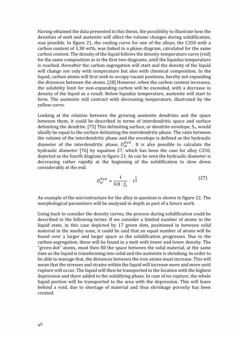
46

Having obtained the data presented in this thesis, the possibility to illustrate how the densities of melt and austenite will affect the volume changes during solidification, was possible. In figure 21, the cooling curve for one of the alloys, the C350 with a carbon content of 3.38 wt%, was linked to a phase diagram, calculated for the same carbon content. The density of the liquid follows the density-temperature curve (red) for the same composition as in the first two diagrams, until the liquidus temperature is reached. Hereafter the carbon segregation will start and the density of the liquid will change not only with temperature but also with chemical composition. In the liquid, carbon atoms will first seek to occupy vacant positions, hereby not expanding the distances between the atoms. [28] However, when the carbon content increases, the solubility limit for non-expanding carbon will be exceeded, with a decrease in density of the liquid as a result. Below liquidus temperature, austenite will start to form. The austenite will contract with decreasing temperature, illustrated by the yellow curve.

Looking at the relation between the growing austenite dendrites and the space between them, it could be described in terms of interdendritic space and surface delimiting the dendrite. [75] This delimiting surface, or dendrite envelope, Sγ, would ideally be equal to the surface delimiting the interdendritic phase. The ratio between the volume of the interdendritic phase and the envelope is defined as the hydraulic diameter of the interdendritic phase, 𝐷𝐷𝐼𝐼𝐼𝐼

𝐻𝐻𝐻𝐻𝐻𝐻 . It is also possible to calculate the hydraulic diameter [76] by equation 27, which has been the case for alloy C350, depicted as the fourth diagram in figure 21. As can be seen the hydraulic diameter is decreasing rather rapidly at the beginning of the solidification to slow down considerably at the end.

𝐷𝐷𝐼𝐼𝐼𝐼𝐻𝐻𝐻𝐻𝐻𝐻 =

10.8 ∙ 𝑓𝑓𝛾𝛾

∙ 𝜕𝜕13 (27)

An example of the microstructure for the alloy in question is shown in figure 22. The morphological parameters will be analysed in depth as part of a future work.

Going back to consider the density curves, the process during solidification could be described in the following terms: If we consider a limited number of atoms in the liquid state, in this case depicted by 17 green dots, positioned in between solid material in the mushy zone, it could be said that an equal number of atoms will be found over a larger and larger space as the solidification progresses. Due to the carbon segregation, these will be found in a melt with lower and lower density. The “green-dot” atoms, must then fill the space between the solid material, at the same time as the liquid is transforming into solid and the austenite is shrinking. In order to be able to manage that, the distances between the iron atoms must increase. This will mean that the stresses and strains within the liquid will increase more and more until rupture will occur. The liquid will then be transported to the location with the highest depression and there added to the solidifying phase. In case of no rupture, the whole liquid portion will be transported to the area with the depression. This will leave behind a void, due to shortage of material and thus shrinkage porosity has been created.


47

Figu

re 2

1. R

elat

ion

betw

een

phas

e di

agra

m, c

oolin

g cu

rve,

den

sity

curv

es a

nd th

e hy

drau

lic d

iam

eter

for a

lloy

C350

.

48

Figure 22. Alloy C350, as cast.


49

CHAPTER 5

CONCLUSIONS

This chapter summarises the work that has been carried out in this thesis and the main conclusions that have been drawn.

Measurement methods and density variation of cast iron in literature

The investigations of the density variations of liquid cast iron are not many in number and the ones found were spread over a long time. Due to the limited number of data, the search had to extended to also include Fe-C alloys, i.e. with little or no silicon. In order to get an overview of available measurement methods, the search had to be widened to include all metals and alloys.

Volume changes and density variations during solidification

Dilatometer measurements could be performed on liquid grey iron, given that the samples were deoxidised with aluminium. It was possible to measure the density variation of the liquid samples in a range from approximately 100 °C above liquidus temperature down to the liquidus temperature.

Two different types of curves could be distinguished (fig.13). The type-I curve, with no clear inflexion point at the presumed liquidus temperature, and the type-II curve with a clear inflexion point at the liquidus temperature. The slopes of these curves could differ markedly.

The slope of the density curves, i.e. the temperature dependence of the density, was calculated in the liquid range and compared to literature values. The slopes were likewise calculated in the austenitic range, however, no literature data could be found to compare with.

Thermal expansion coefficients were measured in both the liquid and the austenitic ranges. It could be established that the thermal expansion coefficients in the austenitic range were approximately twice the value of the ones in the liquid range.

Modelling of density variations and volume change during solidification Using the experimental data, it was possible to build a mathematical model and simulate volume change, with good results. Further development of the model will be the scope of future work. Measurements performed with the sample encased in a container and the temperature measured close to the outer wall of the container will give a value that is either too high or too low compared to the actual temperature of the sample.

50

Compensation must therefore be performed before using the data for further modelling. Compensation should also be made for segregation effects as well as for the presence of a graphite fraction.


51

CHAPTER 6

FUTURE WORK


In this chapter, ideas for future work are presented.

The other varieties of cast iron, i.e. compacted graphite iron and nodular iron, will also undergo the same type of experiments as the lamellar graphite iron in this investigation. This in order to map resemblances and inconsistencies and get a clearer picture of the mechanisms at play in the formation of shrinkage porosity.

From the dilatometer experiments it could be inferred that other properties may play an important part for the outcome of the measurements, it would therefore be a good idea to start to investigate these and to see which impact they have on density. The reasons for the type I and II curves could, for instance, be further looked into. If the shape and the material in the container is the reason or if it has to do with the chemical composition. Additions of deoxidising elements and measurements of the viscosity of liquid cast iron would therefore be examples of areas of interest.

The pressure conditions prevailing during solidification is perhaps hard to measure but is nonetheless very interesting.

Further development of the model and the simulation program lies very close at hand, beginning with establishing a database with temperature dependent values for the density and the specific heat.

Previous researchers [77] have performed element mapping of the areas last to solidify. It would perhaps be a good idea to tailor and cast such compositions and then subject them to testing.


53

REFERENCES

1. Simpson, B.L., History of the Metal Casting Industry. Second ed. ed. 1997, Des Plaines,

Illinois, U.S.A.: American Foundrymen's Society, Inc. 2. Stefanescu, D.M., Computer simulation of shrinkage related defects in metal castings--a review.

International Journal of Cast Metals Research, 2005. 18(3): p. 129-143. 3. Stefanescu, D.M., Principles of the Metallurgy of Cast Iron, in ASM Handbook. 1990 and

2014, ASM International. p. 3-11. 4. Brennert, S., Materiallära. Karlebo. 1993: Liber Utbildning. 5. Minkoff, I. Crystal Growth Theory and Cast Iron Structures. in Physical Metallurgy of Cast

Iron IV. 1989. Tokyo, Japan: Materials Research Society. 6. Vazehrad, S., A Study on Factors Influencing the Microstructure and Shrinkage Porosity

Formation in Compacted Graphite Iron, in Department of Materials Science and Engineering. 2014, Royal Institute of Technology (KTH): Stockholm.

7. Stefanescu, D.M., Science and Engineering of Casting Solidification. Second ed. 2009, New York: Springer.

8. Stefanescu, D.M., et al., The use of combined Liquid Displacement and Cooling Curve Analysis in Understanding the Solidification of Cast Iron. AFS Transactions, 2012(12-045): p. 365-374.

9. Kusakawa, T., S. Kim, and T. Kondo, Volume change of molten spheroidal graphite cast iron. 1972, Report of the Castings Research Laboratory: Waseda University. p. 23-32.

10. Rivera, G., R. Boeri, and J. Sikora, Solidification of gray cast iron. Scripta Materialia, 2004. 50: p. 331-335.

11. Rivera, G.L., R.E. Boeri, and J.A. Sikora. Searching for a Unified Explanation of the Solidification of Cast Irons. in The Eight International Symposium on Science and Processing of Cast Iron. 2006. Beijing, China: Tsinghua University Press.

12. Atkins, P., The laws of thermodynamics. 2010: Oxford University Press. 13. Condensed-Matter Physics. Panel on Condensed-Matter Physics, Physics Survey Committee, Board

on Physics and Astronomy, National Research Council. 1986, National Academy Press: Washington D.C., USA.

14. Schenk, T., et al., Icosahedral Short-Range Order in Deeply Undercooled Metallic Melts. Physical Review Letters, 2002. 89(7): p. 075507-1 - 075507-4.

15. Giancoli, D.C., Physics for Scientists & Engineers. 2008, Upper Saddle River, USA: Pearson Education, Inc./ Prentice Hall.

16. Steinberg, D.J., A Simple Relationship Between the Temperature Dependence of the Density of Liquid Metals and Their Boiling Temperatures. Metallurgical Transactions, 1974. Vol. 5(June): p. 1341-1343.

17. Blumm, J. and J.B. Henderson, Measurement of the volumetric expansion bulk density of metals in the solid and molten regions. High Temperatures--High Pressures (UK), 2000. 32(1): p. 109-113.

18. Jimbo, I. and A.W. Cramb, The Density of Liquid Iron-Carbon Alloys. Metallurgical Transactions B, 1993. 24B: p. 5-10.

19. Brillo, J. and I. Egry, Density of Multicomponent Melts Measured by Electromagnetic Levitation. Japanese Journal of Applied Physics, 2011. 50(11).

20. Mizukami, H., A. Yamanaka, and T. Watanabe, Prediction of density of carbon steels. ISIJ International (Japan), 2002. 42(4): p. 375-384.

54

21. Mills, K.C., Measurement and estimation of physical properties of metals at high temperatures. , in Fundamentals of metallurgy, S. Seetharaman, Editor. 2005, Woodhead Publishing Ltd: Cambridge, England. p. 109-177.

22. Saito, T., Shiraish.Y, and Y. Sakuma, Density measurement of molten metals by levitation technique at temperatures between 1800 degrees C and 2200 degrees C. Transactions of the Iron and Steel Institute of Japan, 1969. 9(2): p. 118-126.

23. Young, H.D. and R.A. Freedman, University Physics. Tenth edition ed. 2000, San Francisco: Addison Wesley Longman.

24. Kirshenbaum, A.D. and J.A. Cahill, The Density of Liquid Iron from the Melting Point to 2500 K. Tranactions of the Metallurgical Society of AIME, 1962. 224(August): p. 816-819.

25. Lucas, L.D., Techniques of Metals Research, in Physiochemical Measurements in Metals Research, R.A. Rapp, Editor. 1970, John Wiley & Sons: New York.

26. Lucas, L.-D., Volume spécifique de métaux et alliages liquides à hautes températures. Première partie. Memoires Scientifiques Rev. Metallurg., 1964. 61(1): p. 1-24.

27. Assael, M.J., et al., Reference Data for the Density and Viscosity of Liquid Aluminum and Liquid Iron. Journal of Physical and Chemical Reference Data, 2006. 35(1): p. 285-300.

28. Olsson, A., The influence of C, Si and Mo on the Density of Liquid Iron. Scandinavian Journal of Metallurgy, 1981. 10: p. 263-271.

29. Langen, M., et al., Measurement of the density and the thermal expansion coefficient of molten silicon using electromagnetic levitation. Journal of Crystal Growth, 1998. 186: p. 550-556.

30. Wille, G., F. Millot, and J.C. Rifflet, Thermophysical Properties of Containerless Liquid Iron up to 2500 K. International Journal of Thermophysics, 2002. 23(5): p. 1197-1206.

31. Gorges, E., et al., Density measurements on levitated liquid metal droplets. International Journal of Thermophysics, 1996. 17(5): p. 1163-1172.

32. Yoo, H., et al., Uncertainty evaluation for density measurements of molten Ni, Zr, Nb and Hf by using a containerless method. Metrologia, 2015. 52(5): p. 677-684.

33. Brillo, J. and I. Egry, Density and excess volume of liquid copper, nickel, iron, and their binary alloys. Zeitschrift Fur Metallkunde, 2004. 95(8): p. 691-697.

34. Smith, P.M., J.W. Elmer, and G.F. Gallegos, Measurement of the density of liquid aluminum alloys by an x-ray attenuation technique. Scripta Materialia, 1999. 40(8): p. 937-941.

35. Mehmood, S., U.E. Klotz, and G. Pottlacher, Thermophysical Properties of Platinum-Copper Alloys. Metallurgical and Materials Transactions, 2012. 43(13): p. 5029-5037.

36. Huepf, T., et al., Thermophysical properties of Ni80Cr20. Thermochimica Acta, 2009. 494(1-2): p. 40-44.

37. Wilthan, B., et al., Thermophysical properties of solid and liquid platinum. Thermochimica Acta, 2004. 415(1–2): p. 47-54.

38. Mohapatra, G., F. Sommer, and E.J. Mittemeijer, The austenite to ferrite transformation of Fe-Ni under the influence of a uniaxially applied tensile stress. Acta Materialia, 2007. 55(13): p. 4359-4368.

39. Yamada, N., R. Abe, and M. Okaji, A calibration method for measuring thermal expansions with a push-rod dilatometer. Measurement Science and Technology (UK), 2001. 12(12): p. 2121-2129.

40. Frankel, J.I., W.D. Porter, and A. Sabau, Analysis of volumetric changes through melting using a dilatometer. Journal of Thermal Analysis and Calorimetry, 2005. 82(1): p. 171-177.

41. Westcot, E.J., C. Binet, and R.M. German, In situ dimensional change, mass loss and mechanisms for solvent debinding of powder injection moulded components. Powder Metallurgy, 2003. 46(1): p. 61-67.


55

42. Kagawa, A., S. Kiguchi, and M. Osada, Volumetric Change in Freezing Cast Irons. Transactions of the Japan Foundrymen's Society, 1995. Vol 18: p. 18-23.

43. Reed, R.C., et al., Determination of reaustenitisation kinetics in a Fe-0.4C steel using dilatometry and neutron diffraction. Materials Science and Engineering A (Switzerland), 1998. 256(1-2): p. 152-165.

44. Sandeep Kumar, T.K., et al., Estimation of Sintering Kinetics of Oxidized Magnetite Pellet Using Optical Dilatometer. Metallurgical and Materials Transactions, 2015. 46(2): p. 635-643.

45. Piasecki, M., et al., Temperature operated infrared nonlinear optical materials based on Tl4HgI 6. Journal of Materials Science. Materials in Electronics, 2013. 24(4): p. 1187-1193.

46. Roach, S.J. and H. Henein, Physical Properties of AZ91D Measured Using the Draining Crucible Method: Effect of SF6. International Journal of Thermophysics, 2012. 33(3): p. 484-494.

47. Roach, S.J. and H. Henein, A new method to dynamically measure the surface tension, viscosity, and density of melts. Metallurgical and Materials Transactions B-Process Metallurgy and Materials Processing Science, 2005. 36(5): p. 667-676.

48. Slack, G.A. and S.F. Bartram, Thermal expansion of some diamondlike crystals. Journal of Applied Physics, 1975. 46(1): p. 89-98.

49. Cottrell, A.H., Theoretical Structural Metallurgy. 1953, London: Edward Arnold & Co. 50. Basic Metallurgy of Cast Iron, in Metals Handbook Desk Edition

J.R. Davis, Editor. 1998, ASM International Handbook Committee. p. 307-309. 51. Goodrich, G.M., Composition of Cast Irons, in ASM Handbook. 2008, ASM

International. p. 785-811. 52. Course on Metallurgy, solidification and modelling of cast iron castings., in Lecture Notes. 2015,

Jönköping University: Jönköping. 53. Elmquist, L., K. Soivio, and A. Diószegi, Cast Iron Solidification Structure and how it is

related to Defect Formation. Materials Science Forum, 2014. 790-791: p. 441-446. 54. Ekbom, L., Grundämnestabell., in MaFyKe. Tabeller och formler N T Te. 1991, Almqvist &

Wiksell: Stockholm. p. 95-97. 55. Ledbetter, H.M. and M.W. Austin, Dilation of an FCC Fe--Cr--Ni Alloy by Interstitial

Carbon and Nitrogen. Mater. Sci. Technol., 1987. 3(2): p. 101-104. 56. Stuart, H. and N. Ridley, Thermal expansion of cementite and other phases. Journal of The

Iron and Steel Institute, 1966. Vol. 204(July): p. 711-717. 57. Chemistry, T.L.B.a.t.R.S.o., A Periodic Table of the Elements. 1987. 58. Silicon (Si), in Encyclopaedia Britannica. Britannica Academic. 20151210, Encyclopædia

Britannica Inc.: http://academic.eb.com/EBchecked/topic/544301/silicon 59. Zulehner, W., B. Neuer, and G. Rau, Silicon, in Ullmann's Encyclopedia of Industrial

Chemistry. 2000, Wiley-VCH Verlag. 60. König, M. and M. Wessén, Influence of alloying elements on microstructure and mechanical

properties of CGI. International Journal of Cast Metals Research, 2010. 23(2): p. 97-110.

61. Chen, Q., E.W. Langer, and P.N. Hansen, Relationship Between Specific Volume, Chemical Composition, and Fraction of Austenite, Graphite and Cementite During Eutectic Reaction of Cast Iron. Scand. J. Metall., 1994. 23(1): p. 3-8.

62. Cockett, G.H. and C.D. Davis, The lattice expansion of Fe-Si alloys and volume change at the A3 point. Journal of the Iron and Steel Institute, 1963. 201(2): p. 110-&.

63. Choe, K.-H., et al., The Effect of Cu on the Microstructure and the Elevated Temperature Properties of Ferritic Heat Resistant Cast Iron. Materials Science Forum, 2010. 654-656: p. 1448-1451.

64. Hummer, R., Relationship between Cooling and Dilatation Curves of Ductile-iron Melts and their Shrinkage Tendency. Cast Metals, 1988. Vol. 1(Number 2).

http://academic.eb.com/EBchecked/topic/544301/silicon

56

65. Ledbetter, H.M. and M.W. Austin, Molybdenum Effect on Volume in Fe--Cr--Ni Alloys. J. Mater. Sci., 1988. 23(9): p. 3120-3124.

66. Hattel, J., Fundamentals of Nummerical Modelling of Casting Processes. 1st ed, ed. J. Hattel. 2005, Kgs. Lyngby, Denmark: Polyteknisk Forlag.

67. Ruhe, A. and G. Söderlind, Numerisk analys., in Nationalencyklopedin. http://www.ne.se/uppslagsverk/encyklopedi/lång/numerisk-analys Acc. 2017-07-31.

68. Lu, X.-G., M. Selleby, and B. Sundman, Theoretical modeling of molar volume and thermal expansion. Acta Materialia, 2005. 53(8): p. 2259-2272.

69. Lucas, L.D., Volume spécifique de métaux et alliages liquides à hautes temperatures. Deuxième partie. Memoires scientifiques rev. metallurg, 1964. 61(2): p. 97-116.

70. Mills, K.C., Recomended Values of Thermophysical Properties for Selected Commercial Alloys. 2002, Cambridge: Woodhead Publishing.

71. Saunders, N., et al., Modelling of the Thermo-Physical and Physical Properties Relevant to Solidification, in Advanced Solidification Processes X, D. Stefanescu, et al., Editors. 2003, TMS.

72. Benedicks, C., N. Ericsson, and G. Ericson, Bestimmung des spezifischen Volumens von Eisen, Nickel und Eisenlegierungen im geschmolzenen Zustand. Archiv für das Eisenhüttenwesen, 1930. 3 Jahrgang(7 (Januar)): p. 473-486.

73. Ash, E.J. and J. Saeger, C.M., Volume changes of cast irons during casting. Bureau of Standards, Journal of Research, 1932. 8(5): p. 601-614.

74. Zhukov, A.A., Thermodynamics of microsegregation and influence of elements on structure of unalloyed and alloyed cast iron. Metal Science 1978. November: p. 521-524.

75. Diószegi, A., V. Fourlakidis, and R. Lora, Austenite dendrite morphology in lamellar graphite iron. International Journal of Cast Metals Research, 2015. 28(5): p. 310-317.

76. Fourlakidis, V., R. Lora, and A. Diószegi, Dynamic coarsening of austenite dendrite in lamellar cast iron part 2 - The influence of carbon composition, in Materials Science Forum. 2014. p. 211-216.

77. Vazehrad, S., J. Elfsberg, and A. Diószegi, Study of microstructure and silicon segregation in cast iron using color etching and electron microprobe analysis. Materials Characterization, 2015. 104: p. 132-138.

http://www.ne.se/uppslagsverk/encyklopedi/l


57

APPENDED PAPERS Supplement I K. Hellström, A. Diószegi and L. Diaconu; A Broad Literature

Review of Density Measurements of Liquid Cast Iron. Published in Metals, 2017, 7(5), 165.

Supplement II K. Hellström, L. Diaconu and A. Diószegi; Density and thermal expansion coefficient of liquid grey cast iron and austenite. Manuscript submitted to Metallurgical and Materials Transactions A.

Supplement III K. Hellström, P. Svidró, L. Diaconu and A. Diószegi; Density variations during solidification of grey cast iron. Presented at the International Symposium on the Science and Processing of Cast Iron (SPCI-XI), 4-7 September 2017 in Jönköping, Sweden

density variations during solidification of lamellar graphite iron1156419/fulltext01.pdf · 2017....

Documents