density-based histogram partitioning and local equalization for...
TRANSCRIPT

Journal of AI and Data Mining
Vol 6, No 1, 2018, 1-12
Density-Based Histogram Partitioning and Local Equalization for
Contrast Enhancement of Images
M. Shakeri, M.-H. Dezfoulian, H. Khotanlou
*
Department of Computer Engineering, Bu-Ali Sina University, Hamedan, Iran.
Receive 10 January 2016; Accepte 08 April 2017
*Corresponding author: [email protected] (H. Khotanlou).
Abstract
Histogram Equalization technique is one of the basic methods available in image contrast enhancement. The
use of this method in the case of images with uniform gray levels (with a narrow histogram) causes the loss
of image details and the natural look of the image. In order to overcome this problem and to have a better
image contrast enhancement, a new two-step method is proposed. In the first step, the image histogram is
partitioned into some sub-histograms according to the mean value and standard deviation, which is
controlled with the PSNR measure. In the second step, each sub-histogram is improved separately and
locally with the traditional histogram equalization. Finally, all sub-histograms are combined to obtain the
enhanced image. The experimental results show that this method would not only keep the visual details of
the histogram but also enhance the image contrast.
Keywords: Contrast Enhancement, Histogram Modification, Image Quality Evaluation, Image Quality
Enhancement.
1. Introduction
Image enhancement methods have been widely
used in many applications of image processing.
Contrast is a main factor in any subjective
evaluation of image quality. Contrast
enhancement is one of the most important areas in
the image processing for human and machine
vision, and many techniques have been proposed
for contrast enhancement and applied to problems
in image processing. This area has great
applications in medical image processing, remote
sensing [1-4], digital photography [5], video
surveillance systems [6], recovery of underwater
visibility [7], and face recognition [8-31].
The histogram modification technique is the most
common method available in image contrast
enhancement, which expands the histogram using
a transfer function [9]. The transfer function can
be used in the global or local mode. In the global
mode, the transfer function is calculated based on
all gray levels in the histogram, while in the local
mode, the transfer function is obtained from a
special interval of histogram [10-13]. Histogram
Equalization is a well-known method in the global
contrast enhancement. Histogram equalization
uses a transfer function based on cumulative
distribution of all intensities in the image.
Histogram equalization is not suitable for keeping
the mean brightness of the image, and causes
intensity saturation problems [14]. In [14], Kim
has proposed a method called BBHE, which is
based upon histogram equalization on each one of
the two sub-histograms that are separated by the
mean value. In the output images of the BBHE
method, the over-enhanced regions can be seen
due to the application of only one separation on
the histogram. In [15], Wang has presented a
method called DSIHE. In this method, in the first
step, the histogram is divided into two equal sub-
histograms based on the middle value of gray
levels. Then the histogram equalization is applied
to each sub-histogram. Since DSIHE divides the
histogram into just two sub-histograms, this
method has the same problem of BBHE. In order
to overcome this problem, Sim presented the
RSIHE method in [16] based on DSIHE. The
RSIHE method, in a recursive operation, divides
the histogram of the image into two equal sub-
histograms. This operation is repeated for r times.

Khotanlou et al. / Journal of AI and Data Mining, Vol 6, No 1, 2018.
2
The histogram is divided into 2r sections, and then
the histogram equalization is applied for each sub-
histogram. A large r is suitable for preserving
mean brightness but there is no special
enhancement. With a small r, this method operates
similar to DSIHE.
In [25], the bi-histogram equalization plateau limit
(BHEPL) has been proposed to control the BBHE
enhancement rate. BBHE applies a higher
stretching process to the contrast of the high-
histogram regions and compresses the contrast of
the low histogram regions, possibly causing
intensity saturation in the low histogram regions.
A clipping process is applied to each sub-
histogram of BBHE to deal with the intensity
saturation problem and to control the
enhancement rate through setting the plateau limit
as the average number of intensity occurrence. If
the bins for any intensity exceed the plateau limit,
they are replaced by the plateau limit level;
otherwise, they remain the same as the original
bins of the input histogram. Finally, HE is
implemented to the clipped sub-histograms.
In [17], Draa has proposed a method based on
finding the best transfer function using the
Artificial Bee Colony (ABC) algorithm with a
fitness function based on entropy and Sobel
operator. In [21], Pourya Hoseini has proposed a
hybrid algorithm including Genetic Algorithm
(GA), Ant Colony Optimisation (ACO), and
Simulated Annealing (SA) metaheuristics for
increasing the contrast of images. Ant colony
optimization is used to generate the transfer
functions, which map the input intensities to the
output one. Simulated annealing, as a local search
method, is utilized to modify the transfer
functions generated by ant colony optimization.
Genetic algorithm has the responsibility of
evolutionary process of ants’ characteristics.
In [18], Khan has proposed a method based on the
local histogram equalization. In this method, the
image histogram is divided into several parts
according to the middle and mean values. The
narrow areas of the histogram are then discovered
and are expanded to a full brightness area, like in
the HE method.
After equalization of every part with the HE
method, the image is normalized in order to
prevent the brightness saturation issues. In [19],
Huang has proposed a method in which, according
to the mean value of image, the histogram is
divided into several parts, and the histogram
equalization is then applied for each part. In this
method, after histogram equalization, the image
details would be lost due to some large divisions
and lots of changes in brightness.
In [24], Huang has proposed a combinatorial
method, which contains the gamma correction and
the traditional histogram equalization. This
method has created a balance between a high level
of visual quality and a low computational cost.
Gu [26] has used saliency preserving to increase
the image contrast without dealing with the
artifact problem. The proposed framework
includes the histogram equalization and its
relevant visual pleasing conducted by the sigmoid
function. Finally, this method exploits a quality
determination measure based upon saliency
preserving to automatically select parameters.
In [27], a method has been proposed to avoid
over-enhancement and noise addition, while
improving the contrast of an image. The method is
a combination of Contrast Limit Adaptive
Histogram Equalization (CLAHE) and Discreet
Wavelet Transform (DWT). High frequencies of
the image and its low counterparts are first
decomposed by DWT. The image frequency
coefficients are equalized by CLAHE, while
leaving image high frequency with no alteration.
Eventually, the reverse DWT is employed to
reconstruct the image. In the last step, a weighted
factor is obtained from the original and the
enhanced image to control the possible over-
enhancement.
Estimating and compressing the illumination
component is a good method to enhance the
degraded images by an uneven light. In [28],
Liang has proposed a novel method to estimate
the illumination by an iterative solution of non-
linear diffusion equation.
In [29], Celik has proposed a new algorithm to
enhance images using special information of
pixels. This algorithm computes the spatial
entropy of pixels by considering the distribution
of spatial locations of gray levels.
In the proposed method, which is based on [19],
the histogram is divided into several optimal parts
according to density, mean, and standard
deviation of image intensities. Then the large
sections are identified and again divided into
several parts. Finally, the enhanced image is
constructed with local histogram equalization. The
results obtained show that this method not only
keeps the pixel mean and features but also
enhances the image contrast.
2. Proposed method
One of the common methods used for enhancing
image contrast is an approach based on histogram
modification. These methods map image pixels
aiming at expanding image histogram using a
transfer function. The transfer function used for

Khotanlou et al. / Journal of AI and Data Mining, Vol 6, No 1, 2018.
3
enhancing image contrast can be in two modes;
global and local. In the global mode, the transfer
function is calculated in proportion to the entire
histogram. In the local mode, this transferring
function is applied for a special interval of
histogram. The proposed method is divided into
two parts.
The first part is histogram division, and the
histogram is divided into parts to calculate the
transfer function locally. The second part is the
local equalization of histogram. One of the
famous methods used for contrast enhancement is
the histogram equalization method. Histogram
equalization produces an image whose density
levels of brightness are uniform, resulting in an
increase in the pixel intervals, which has a
considerable effect on the image quality. In this
part, the actions of histogram equalization in local
mode are discussed.
2.1. Histogram division
In this part, the image histogram is divided
according to diffusion of the existing brightness
levels in the image. If the brightness values for the
image are in the [a,b] interval, H(i), i = a, a + 1, a
+ 2, …, b, indicates the number of image pixels
with an i brightness level. In fact, H is the
histogram function of the image brightness level.
Based on this, the mean and standard deviation of
the image brightness value are calculated using
(1) and (2).
b
i a
b
i a
H i *i
H(i)
(1)
1/2
b2
bi a
i a
1 H(i)(i - )
H(i) -1
(2)
The algorithm of histogram division is:
Algorithm 1: Suppose that the brightness level
value of image is in [0,255].
In the first step, initialize a = 0 and b = 255.
Mean and standard deviation of image are
calculated in [a,b].
Two threshold values to separate and divide the
histogram are calculated by (3) and (4).
1T - (3)
2T - (4)
Now, [a,T1] and [T2,b] are two parts of the
histogram that are stored.
In this step, to divide [T1,T2] into smaller parts,
we replace the pixels values of the image that
were in [a,T1] with mean pixel value of [a,T1].
Also we replace the pixel values of the image in
[T2,b] with the mean pixels value of [T2,b] ((5)
and (6)). 1T
i a
1
i *H(i)
T - a
(5)
2
b
i T
2
i *H(i)
b - T
(6)
Put the “a” value equal to T1 + 1 and “b” equal
to T2 – 1, and repeat the algorithm from step 2.
The stopping criterion of this loop is that the
difference between the image PSNR criteria for
two successive steps would be more than 0.1.
Otherwise, this image can be still divided into
smaller intervals. 0.1 is obtained experimentally.
PSNR is most commonly used to measure the
quality of reconstruction of lossy compression
codecs. Since histogram division is a kind of
compression, and has less complexity, we use the
PSNR measure to compute the similarity of two
images. PSNR is a criterion that shows the ratio
between the peak possible power of signal and the
noise failure power and its effects on displaying
signal. In fact, it calculates the similarity of two
images, and its value is calculated as follows ((7)
and (8)).
10
255PSNR 20 *log
RMSE (7)
M-1 N-12 1/2
xy xy
x 0 y 0
1RMSE ( [I - I ] )
MN
(8)
I and I’ show the mean level of the original and
enhanced image with M*N pixels. RMSE is the
root of mean square error, and is calculated from
the difference between the estimated values by the
model and real observed values. The output of this
step is shown in figure 1. In the i’th step of
applying algorithm 1, where i = 1, 2, …, t, the two
[a(i)
,T1(i)
] and [T2(i)
,b(i)
] intervals are stored in S
matrix. t is a step, in which the difference value of
PSNR between t and t-1 is greater than 0.1, and S
matrix indicates dividing intervals of the
histogram in algorithm 1. Different steps of
algorithm 1 are shown in a diagram in figure 8a.
Figure 4 shows the divided histogram and
obtained intervals with algorithm 1 for figure 9a.
In this figure, t or steps of algorithm would be
equal to 3.
As it can be seen in figure 4, based on density,
mean, and standard deviation, algorithm 1 divides
the histogram into intervals but some of the
selected intervals, which are shown in figure 4
with arrows, have covered a vast scope of the
histogram. This causes an increasing brightness
value change in these intervals in the local

Khotanlou et al. / Journal of AI and Data Mining, Vol 6, No 1, 2018.
4
histogram equalization step, failure to maintain
image mean, and loss of some image features
(Figure 5). As specified in figure 5, in great
intervals (two intervals have been shown), the
brightness changes are too much and the image
details would disappear (shown in the results
section).
1 1
1
2 2
1
1 1 t t
1 2 t t
12 2
1 t t
2 2 1 2
2 t t
t t 1 1 2
1 2
2 2
2
1 1
2
a T
a T
a T T ba T
a T, S= T +1 T -1
T bT b
a T T b
T b
T b
Figure 1. intervals obtained from implementation of
algorithm 1.
In order to overcome this problem, it is necessary
to prevent the creation of great intervals.
Considering a constant value of p as a threshold
value for each pair of consecutive intervals in S
that has a difference greater than p is a solution.
Algorithm1 can again be applied for the original
(input) image. However, the stopping condition,
PSNR criterion, should be greater than 0.1 in the
two consecutive algorithm steps and the
difference between a and b should be greater than
the threshold value for p in each step. Thus:
If the difference between T1(i)
and a(i)
, i =
1,2,…,t, is greater than p, algorithm 1 in step 2
starts with the values a = a(i)
and b = T1(i)
, and
the intervals obtained, like the structure in
figure 1, would be added to the new T set.
Otherwise, [a(i)
, T1(i)
] would be added to the T
set.
The [T1(t)
+1 , T2(t)
-1] interval is added to the T
set.
Accordingly, for the second section of S, if the
difference between b(i)
and T2(i)
, i = 1,2,…,t, is
greater than p, algorithm 1 of step 2 is carried
out with starting values of a = T2(i)
and b = b(i)
,
and the intervals obtained with structures like
that in figure 1 would be added to the T set;
otherwise, [T2(i)
, b(i)
] would be added to the T
set.
After this procedure with p parameter greater than
50, the histogram intervals of figure 9a would be
as in figure 6. As observed, with re-
implementation of algorithm 1, the intervals
greater than 50 in figure 4 are divided into smaller
intervals, based on mean and variance (Figure 6).
This procedure causes the mean brightness pixels
to be more preserved after the histogram local
equalization, which is applied for each interval.
Figure 7 shows that selecting smaller intervals
causes histogram uniformity, and the mean
brightness of pixels is completely preserved
(enhanced image is shown in the results section).
In figure 8b, the diagram of steps of re-division of
histogram by algorithm 1 and the place of
histogram equalization are shown. In order to
determine the optimum value for the PSNR
threshold and “p”, four images were analyzed.
Figure 2 shows the PSNR threshold to number of
sub-histograms ratio. For values greater than 0.1,
the number of sub-histograms does not change too
much.
Figure 2. PSNR threshold to number of sub-histograms
ratio.
Figure 3 shows the “p” value to number of sub-
histograms greater than “p” ratio. For values
bigger than 50, the number of sub-histograms
greater than “p” reaches zero, which makes the
proposed method ineffective.
Figure 3. Value of “p” to number of sub-histogram
greater than “p” ratio.
2.2. Local Equalization of Histogram
Up to this point, image histogram is partitioned
into parts, and the existing intervals are obtained
in set T. We will save the number of produced
intervals via the previous step algorithm, in e
parameter.
The method of histogram local equalization is as
follows:
0
2
4
6
8
10
12
14
16
0.01 0.05 0.1 0.5 1 10 50 100
Nu
mb
er o
f su
b-h
isto
gra
ms
Value of PSNR threshold
Girl Boat Couple Plane
0
1
2
3
4
5
6
7
10 20 30 40 50 60 80 100 120 160
Nu
mb
er o
f su
b-h
isto
gra
ms
gre
ater
th
an p
Value of p
Girl Boat Couple Plane

Khotanlou et al. / Journal of AI and Data Mining, Vol 6, No 1, 2018.
5
First, for each e interval of the histogram, in the
original (input) image, the probability density
function is calculated based on (9).
k i
ii
npdf i
n
(9)
k 1, 2, , e ,
i T k,1 , T k,1 1 , T k,1 2 , , T(k, 2)
i is the brightness level in the k’th interval; the
first index of the T set shows row, and the second
index shows column. ni also shows the number of
i brightness levels in the original image. Also the
cumulative distribution function (CDF) is
calculated for each part of the histogram in the
original image by (10).
i
k k
h T k,1
cdf i pdf h
(10)
k 1, 2, , e ,
i T k,1 , T k,1 1 , T k,1 2 , , T(k, 2)
i is the brightness level in the k’th interval; the
first index of the T set shows row, and the second
index shows column. Using a mapping function,
and applying k’th cdf on the k’th interval of the
original image (sub-image), we will reach the
enhanced image with (11).
k kP i T k,1 T k,2 - T k,1 * cdf (i) (11)
k 1, 2, , e ,
i T k,1 , T k,1 1 , T k,1 2 , , T(k, 2)
Pk(i), in fact, is the histogram value in the k’th
interval of brightness level of i in the
original image.
Figure 4. Histogram divisions and the obtained intervals
by initial implantation of algorithm1.
3. Results
In this part, the proposed methods will be
compared with the other methods. The results of
test with parameter p = 50 were evaluated in two
cases.
3.1. Qualitative evaluation
Different contrast enhancement algorithms are
evaluated for four famous image visually. Figure
9a shows the image that the histogram
equalization algorithm is applied to, where there
are lots of inconsistencies among background,
hair, body, and face in the two original and
enhanced images. Results of the BBHE, DSIHE,
and RSIHE algorithms are shown in figure 9c,
figure 9f, and figure 9b, respectively. These
methods use the local sub-histograms for
decreasing the histogram equalization effect but
many result aspects still exis as a result of
applying the histogram equalization in these
methods. For example, hair and clothes are rather
dark, face is too bright, there are lots of changes in
the pixel brightness values, and therefore, lots of
image details have been lost.
Figure 5. Results of applying local histogram equalization
on initial intervals by algorithm 1 on Figure 9a.
𝑇 =
0 5455 96
97 110111 133134 140𝟏𝟒𝟏 𝟏𝟒𝟓146 149150 168169 183184 194195 236237 241242 255
[𝑇1(𝑡)
+ 1 𝑇2(𝑡)
− 1]
Figure 6. Histogram divisions and intervals obtained on
Figure 9a after re-implantation of algorithm 1 for
intervals larger than p.

Khotanlou et al. / Journal of AI and Data Mining, Vol 6, No 1, 2018.
6
Figure 7. Result of local histogram equalization on
secondary intervals formed by re-implantation of
algorithm 1 on Figure 9a.
In figure 9g, the results of applying algorithm [19]
can be seen where somehow the mean of image
brightness is preserved and great enhancement is
applied. However, due to the long length of some
intervals, some image details have been lost; for
example, hair area is completely dark.
In figure 9i, the result of SDDMHE method is
shown, which is not enhanced enough. In figure
9h, the enhanced image from the proposed
algorithm has been shown. Because of using the
local sub-histograms with optimum intervals, in
addition to enhanced contrast, the mean value of
pixels is preserved, and therefore, none of the
image details have been lost; for example, hair
area seems more natural. Also figure 9d shows the
result of the ABC method that presents the same
enhanced results with the proposed method,
except the bow tie and face area. Also in figures
10 and 11, the proposed ABC and RSIHE
methods; and in figure 12, the proposed method
generate the best output image.
If you choose not to use this document as a
template, prepare your technical work in single-
spaced, double-column format. Set bottom
margins to 25 millimeters (0.98 inch) and top, left
and right margins to about 20 millimeters (0.79
inch). Margin of First page is different from other
pages. For first page set top margin to 30
millimeters (1.18 inch), and bottom, left and right
margins are similar to other pages. Do not violate
margins (i.e., text, tables, figures, and equations
may not extend into the margins). The column
width is 78 millimeters (3.07 inches). The space
between the two columns is 13 millimeters (0.51
inch).
3.2. Quantitative evaluation
In addition to the qualitative evaluation,
measuring the accuracy is one of the requirements
to compare the proposed method and the other
existing methods.
There are five measuring criteria used in this
paper: PSNR, AMBE [20], FSIM [22], KL[30]
distance, and DE [23].
AMBE is the absolute difference between the
mean values of input image X and output image Y
to define the normalized absolute mean brightness
error (12) (AMBE ∈ [0,1]).
1AMBE X,Y
1 MB X - MB Y
(12)
where, MB(X) and MB(Y) are the average values
of X and Y, respectively. In table 1, the AMBE
values for the contrast enhancement methods are
shown on 10 images. The proposed ABC and
SDDMHE methods can completely preserve the
mean values of image pixels because they use the
local histogram equalization with optimum
intervals instead of the global histogram
equalization. Therefore, they can effectively
decrease AMBE. Table 2 shows the PSNR values
obtained by applying a different algorithm on the
previous images. We can see that the PSNR
values obtained by the proposed method have
maximum values. A greater PSNR value indicates
that there is more similarity between the original
and enhanced images. Histogram equalization
refers to processing the input image to utilize the
dynamic range efficiently by mapping an input
into output image such that there is an equal
number of pixels at each grey-level in the output.
Thus it is expected that the equalized output
image has flattened the grey-level distribution.
However, it should be noted that the process
should not change the overall shape of the input
histogram to protect the image content. In order to
quantitatively measure how flattened the output
grey-level distribution is, the Kullback–Leibler
(KL) distance between the distribution of the
processed output image p(yk) and the uniform
distribution q(yk) was used. The KL-distance (13)
is a natural distance function from a “true”
probability distribution, p(yk), to a “target”
probability distribution, q(yk).
kk 2
k k
p(y )KL p,q p(y )log
q(y )
(13)
The lower the value of KL, the better the
histogram equalization is. Table 3 shows that the
proposed method output generates the lowest KL-
distance between other methods.
Another quantitative evaluation is the discrete
entropy (DE). The discrete entropy of the input
image X with K distinct grey-levels is in (14).
K
k k
k 1
DE X - p x log p x
(14)

Khotanlou et al. / Journal of AI and Data Mining, Vol 6, No 1, 2018.
7
where, p(xk) is the probability of pixel intensity
xk, which is estimated from the normalized
histogram. Similarly, the discrete entropy of the
output image Yw with L distinct grey-levels is
defined as (15).
L
w l l
l 1
DE(Y ) - p y log p y
(15)
where, p(yl) is the probability of pixel intensity yl.
A higher value of DE indicates that the image has
richer details. Using the metrics DE(X) and
DE(Yw), the normalized discrete entropy
(DEN(X,Yw) ∈ [0,1]) between the input image X
and the output image Yw is defined as (16).
N w
w
1DE X,Y
log 256 - DE Y1
log 256 - DE X
(16)
where, log(256) is the maximum value of entropy
that can be achieved using the 8-bits data
representation. The higher the value of normalized
discrete entropy, the better the enhancement is in
terms of utilizing the dynamic range and
providing better image details. Table 4 shows the
DE value for different algorithms.
The visual information in an image is often very
redundant, while HVS understands an image
mainly based on its low-level features.
Table 1. Comparing various methods with AMBE.
Test Images HE BBHE DSIHE [21] [19] Proposed RSIHE SDD
MHE ABC
baboon 0.0673 0.0796 0.0652 0.3382 0.0813 0.1816 0.1383 0.4077 0.1296
boat 0.0447 0.3169 0.0213 0.3637 0.0708 0.4878 0.2756 0.1442 0.3584
City 0.0145 0.0503 0.0137 0.0347 0.1267 0.5220 0.1599 0.3816 0.2209
Couple 0.1884 0.1051 0.1092 0.3665 0.2765 0.9831 0.3293 0.6331 0.6260
Girl 0.0565 0.0474 0.0390 0.1007 0.2899 0.6501 0.2898 0.4218 0.3858
Jet 0.0194 0.3142 0.1232 0.0473 0.1490 0.4975 0.1566 0.2983 0.2002
Lenna 0.2249 0.1146 0.3467 0.1416 0.1313 0.9657 0.2057 0.6089 0.4375
Man 0.0252 0.0400 0.0220 0.0445 0.1204 0.2735 0.1325 1.3892 0.9874
Peppers 0.0599 0.1392 0.1615 0.2256 0.1665 0.3582 0.1467 0.4971 0.2245
Plan 0.0205 0.3762 0.1197 0.0315 0.3680 0.4284 0.2349 0.2148 0.1977
Average 0.0721 0.1584 0.1022 0.1694 0.1780 0.5348 0.2069 0.4997 0.3768
Table 2. Comparing various methods with PSNR.
Test Images HE BBHE DSIHE [21] [19] Proposed RSIHE SDD
MHE ABC
baboon 18.23 18.56 13.97 22.20 26.24 30.80 23.64 27.64 18.91
boat 17.97 18.14 13.08 18.56 24.13 32.83 32.82 31.13 18.47
City 11.03 16.38 10.50 15.58 20.64 32.92 22.66 29.85 20.90
Couple 17.22 17.26 14.20 17.69 22.59 30.58 28.10 28.10 17.55
Girl 13.85 14.60 17.77 16.68 20.15 35.16 30.12 30.28 23.96
Jet 12.84 21.91 16.87 18.82 27.32 34.28 26.04 28.43 21.89
Lenna 20.13 20.15 21.95 24.01 28.98 27.33 25.23 31.23 24.63
Man 16.53 19.09 14.38 19.84 23.28 34.03 25.38 28.14 18.03
Peppers 20.35 21.75 21.13 26.85 31.36 26.18 26.21 30.55 21.20
Plan 10.23 14.29 19.02 13.20 18.80 36.09 33.66 31.28 27.90
Average 15.84 18.21 16.29 19.34 24.35 32.02 27.39 29.66 21.34
Table 3. Comparing various methods with KL.
Test Images HE BBHE DSIHE [21] [19] Proposed RSIHE SDD
MHE ABC
baboon 2.0242 1.6299 0.7356 0.7242 0.7142 0.3449 0.7736 0.9156 0.7613
boat 2.0464 2.1224 1.0737 1.0394 0.9349 0.4332 1.004 1.1302 0.5865
City 2.0721 1.7622 1.2515 1.2133 1.1363 0.9895 1.1606 1.4986 0.5757
Couple 2.0408 1.5532 1.0101 0.9909 0.9307 0.5226 0.9379 1.1099 0.7561
Girl 3.1498 3.8185 2.8002 2.5443 2.4394 1.7853 2.5175 2.7288 2.1528
Jet 2.2886 2.0348 1.4453 1.4004 1.4258 0.7586 1.4959 1.7674 4.4943
Lenna 2.0307 1.2927 0.73 0.659 0.6627 0.4748 0.6915 0.8386 0.2135
Man 2.0486 1.065 0.709 0.7335 0.638 0.3984 0.6771 0.6962 0.6952
Peppers 2.0267 0.6835 0.6313 0.6029 0.595 0.6256 0.6197 0.7135 0.4291
Plan 4.2533 4.2304 4.32 4.0942 4.0119 3.0112 4.0353 3.9958 3.0218
Average 2.3981 2.0193 1.4707 1.4002 1.3489 0.9344 1.3913 1.5395 1.3686
In other words, the salient low-level features
convey crucial information for HVS to interpret
the scene. Accordingly, perceptible image
degradations will lead to perceptible changes in
image low-level features, and hence, a good IQA
metric could be devised by comparing the low-
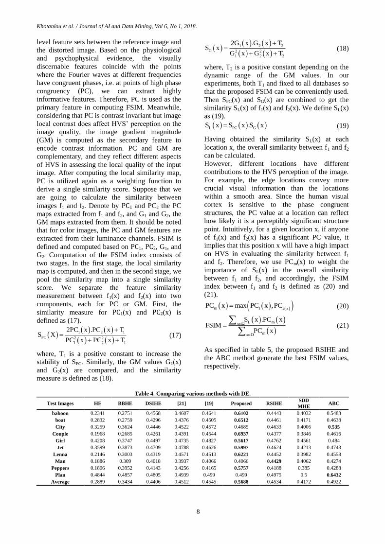
Khotanlou et al. / Journal of AI and Data Mining, Vol 6, No 1, 2018.
8
level feature sets between the reference image and
the distorted image. Based on the physiological
and psychophysical evidence, the visually
discernable features coincide with the points
where the Fourier waves at different frequencies
have congruent phases, i.e. at points of high phase
congruency (PC), we can extract highly
informative features. Therefore, PC is used as the
primary feature in computing FSIM. Meanwhile,
considering that PC is contrast invariant but image
local contrast does affect HVS’ perception on the
image quality, the image gradient magnitude
(GM) is computed as the secondary feature to
encode contrast information. PC and GM are
complementary, and they reflect different aspects
of HVS in assessing the local quality of the input
image. After computing the local similarity map,
PC is utilized again as a weighting function to
derive a single similarity score. Suppose that we
are going to calculate the similarity between
images f1 and f2. Denote by PC1 and PC2 the PC
maps extracted from f1 and f2, and G1 and G2, the
GM maps extracted from them. It should be noted
that for color images, the PC and GM features are
extracted from their luminance channels. FSIM is
defined and computed based on PC1, PC2, G1, and
G2. Computation of the FSIM index consists of
two stages. In the first stage, the local similarity
map is computed, and then in the second stage, we
pool the similarity map into a single similarity
score. We separate the feature similarity
measurement between f1(x) and f2(x) into two
components, each for PC or GM. First, the
similarity measure for PC1(x) and PC2(x) is
defined as (17).
1 2 1
PC 2 2
1 2 1
2PC x .PC x TS X
PC x PC x T
(17)
where, T1 is a positive constant to increase the
stability of SPC. Similarly, the GM values G1(x)
and G2(x) are compared, and the similarity
measure is defined as (18).
1 2 2
G 2 2
1 2 2
2G x .G x TS x
G x G x T
(18)
where, T2 is a positive constant depending on the
dynamic range of the GM values. In our
experiments, both T1 and fixed to all databases so
that the proposed FSIM can be conveniently used.
Then SPC(x) and SG(x) are combined to get the
similarity SL(x) of f1(x) and f2(x). We define SL(x)
as (19).
L PC GS x S x .S x (19)
Having obtained the similarity SL(x) at each
location x, the overall similarity between f1 and f2
can be calculated.
However, different locations have different
contributions to the HVS perception of the image.
For example, the edge locations convey more
crucial visual information than the locations
within a smooth area. Since the human visual
cortex is sensitive to the phase congruent
structures, the PC value at a location can reflect
how likely it is a perceptibly significant structure
point. Intuitively, for a given location x, if anyone
of f1(x) and f2(x) has a significant PC value, it
implies that this position x will have a high impact
on HVS in evaluating the similarity between f1
and f2. Therefore, we use PCm(x) to weight the
importance of SL(x) in the overall similarity
between f1 and f2, and accordingly, the FSIM
index between f1 and f2 is defined as (20) and
(21).
m 1 2 xPC x max PC x ,PC (20)
L mx
mx
S x .PC xFSIM
PC x
(21)
As specified in table 5, the proposed RSIHE and
the ABC method generate the best FSIM values,
respectively.
Table 4. Comparing various methods with DE.
Test Images HE BBHE DSIHE [21] [19] Proposed RSIHE SDD
MHE ABC
baboon 0.2341 0.2751 0.4568 0.4607 0.4641 0.6102 0.4443 0.4032 0.5483
boat 0.2832 0.2759 0.4296 0.4376 0.4505 0.6512 0.4461 0.4171 0.4638
City 0.3259 0.3624 0.4446 0.4522 0.4572 0.4685 0.4633 0.4006 0.535
Couple 0.1968 0.2685 0.4261 0.4391 0.4544 0.6937 0.4377 0.3846 0.4616
Girl 0.4208 0.3747 0.4497 0.4735 0.4827 0.5617 0.4762 0.4561 0.484
Jet 0.3599 0.3873 0.4709 0.4788 0.4626 0.5997 0.4624 0.4213 0.4743
Lenna 0.2146 0.3003 0.4319 0.4571 0.4513 0.6221 0.4452 0.3982 0.4558
Man 0.1886 0.309 0.4018 0.3937 0.4066 0.4066 0.4429 0.4062 0.4274
Peppers 0.1806 0.3952 0.4143 0.4256 0.4165 0.5757 0.4188 0.385 0.4288
Plan 0.4844 0.4857 0.4805 0.4939 0.499 0.499 0.4975 0.5 0.6432
Average 0.2889 0.3434 0.4406 0.4512 0.4545 0.5688 0.4534 0.4172 0.4922

Khotanlou et al. / Journal of AI and Data Mining, Vol 6, No 1, 2018.
9
Table 5. Compare various method with FSIM.
Test Images HE BBHE DSIHE [21] [19] Proposed RSIHE SDD
MHE ABC
baboon 0.8395 0.9365 0.8936 0.9571 0.9449 0.9929 0.9194 0.8947 0.9194
boat 0.6859 0.8236 0.8077 0.9208 0.8889 0.9933 0.9829 0.8728 0.983
City 0.7566 0.8328 0.7893 0.9173 0.8858 0.9863 0.9907 0.8407 0.9382
Couple 0.8938 0.8205 0.8137 0.9044 0.8838 0.9895 0.9577 0.8192 0.9577
Girl 0.5737 0.6302 0.5986 0.7161 0.8377 0.9732 0.962 0.6521 0.9692
Jet 0.8464 0.8744 0.7514 0.9595 0.9196 0.9795 0.9965 0.9185 0.9648
Lenna 0.9112 0.9576 0.9284 0.9729 0.9328 0.99 0.9561 0.9321 0.9561
Man 0.9165 0.9377 0.9486 0.947 0.9521 0.9874 0.9889 0.9366 0.9599
Peppers 0.9476 0.967 0.9479 0.9798 0.9709 0.99 0.9595 0.9454 0.9603
Plan 0.5057 0.6026 0.5681 0.7403 0.9066 0.9708 0.9777 0.6207 0.9773
Average 0.7877 0.8383 0.8047 0.9015 0.9123 0.9853 0.9691 0.8433 0.9586
a b
Input
Image
Acquire and Save
Calculate
Difference of
PSNR
Generate S
and i=1
Acquire and Save
𝑖 = 𝑖 + 1
𝑖 ≤ 𝑒
Implement Local
Histogram Equalization
On Original Image
According To Intervals
In T
Enhance
Output
Image
0.1>
>0.1
Yes
No
Yes
No
𝑎 = 0 , 𝑏 = 255
Calculate
Difference of
PSNR
0.1> >0.1
Yes
No
[𝑎, 𝑇1] , [𝑇2 , 𝑏]
[𝑎, 𝑇1] , [𝑇2 , 𝑏]
𝑎 = 𝑆( 𝑖 , 1 ) , 𝑏 = 𝑆( 𝑖 , 2)
Save
S(i,2) and S(i,1) in T
𝑏 − 𝑎 > 𝑝
𝑏 − 𝑎 > 𝑝
Figure 8. (a) Algorithm 1 steps (b) steps of re-implantation of algorithm 1 for intervals. larger than p.
Figure 9. Girl (a) The original Image, The experimental image under study (b) The enhanced image by Histogram
Equalization (c) The enhanced image by BBHE (d) The enhanced image by ABC (e) the enhanced image by RSIHE (f) The
enhanced image by DSIHE (g) The enhanced image by [19] (h) The enhanced image by the proposed method (i) The
enhanced image by SDDMHE (j) The enhanced image by [21].
4. Conclusion
In this paper, a new method was proposed for
image contrast enhancement without losing image
details. Intensity saturation and over-enhancement
is one of the main issues in the other proposed
contract enhancement methods. In order to
overcome this problem and also to obtain a
desired contrast enhancement, the image
histogram is first divided into some sub-
histograms according to the mean value and
standard deviation. Then every single sub-
histogram is enhanced separately using the
traditional histogram equalization. Finally, these
enhanced sub-histograms are combined to make
the enhanced image. The qualitative and
quantitative results of comparing different
contrast enhancement methods with the proposed
method show that the proposed method not only
keeps the details and image brightness level mean
but also enhances the image contrast effectively,
and leads to an increased image quality. Selecting
the parameters related to the number of sub-
(b) (c) (d) (e)
(f) (g) (h) (i) (j)
(a)

Khotanlou et al. / Journal of AI and Data Mining, Vol 6, No 1, 2018.
10
histograms was one of the problems faced with in
this work. A solution is using a method to obtain
the value of “p” and PSNR threshold according to
the input image.
Figure 10. Boat (a) Original Image (b) Enhanced image by Histogram Equalization (c) Enhanced image by BBHE (d)
Enhanced image by ABC (e) Enhanced image by RSIHE (f) Enhanced image by DSIHE (g) Enhanced image by [19] (h)
Enhanced image by proposed method (i) Enhanced image by SDDMHE (j) Enhanced image by [21].
Figure 11. Couple (a) Original Image (b) Enhanced image by Histogram Equalization (c) Enhanced image by BBHE (d)
Enhanced image by ABC (e) Enhanced image by RSIHE (f) Enhanced image by DSIHE (g) Enhanced image by [19] (h)
Enhanced image by proposed method (i) Enhanced image by SDDMHE (j) Enhanced image by [21].
Figure 12. Plan (a) Original Image (b) Enhanced image by Histogram Equalization (c) Enhanced image by BBHE (d)
Enhanced image by ABC (e) Enhanced image by RSIHE (f) Enhanced image by DSIHE (g) Enhanced image by [19] (h)
Enhanced image by proposed method (i) Enhanced image by SDDMHE (j) Enhanced image by [21].
(a) (b) (c) (d) (e)
(f) (g) (h) (i) (j)
(a) (b) (c) (d) (e)
(f) (g) (h) (i) (j)
(a) (b) (c) (d) (e)
(f) (g) (h) (i) (j)

Khotanlou et al. / Journal of AI and Data Mining, Vol 6, No 1, 2018.
11
References [1] Chen, C. Y., Lin, T. M., & Wolf, W. H. (2008). A
visible/infrared fusion algorithm for distributed smart
cameras. IEEE Journal of Selected Topics in Signal
Processing, vol. 2, no. 4, pp. 514-525.
[2] Lai, C. C., & Tsai, C. C. (2008). Backlight power
reduction and image contrast enhancement using
adaptive dimming for global backlight applications.
IEEE Transactions on Consumer Electronics, vol. 54,
no. 2, pp. 669-674.
[3] Kim, Y. T. (1997). Contrast enhancement using
brightness preserving bi-histogram equalization. IEEE
transactions on Consumer Electronics, vol. 43, no. 1,
pp. 1-8.
[4] Kim, J. Y., Kim, L. S., & Hwang, S. H. (2001). An
advanced contrast enhancement using partially
overlapped sub-block histogram equalization. IEEE
transactions on circuits and systems for video
technology, vol. 11, no. 4, pp. 475-484.
[5] Wang, Y., Chen, Q., & Zhang, B. (1999). Image
enhancement based on equal area dualistic sub-image
histogram equalization method. IEEE Transactions on
Consumer Electronics, vol. 45, no. 1, pp. 68-75.
[6] Sim, K. S., Tso, C. P., & Tan, Y. Y. (2007).
Recursive sub-image histogram equalization applied to
gray scale images. Pattern Recognition Letters, vol. 28,
no. 10, pp. 1209-1221.
[7] Xie, X., & Lam, K. M. (2005). Face recognition
under varying illumination based on a 2D face shape
model. Pattern Recognition, vol. 38, no. 2, pp. 221-
230.
[8] van Bemmel, C. M., Wink, O., Verdonck, B.,
Viergever, M. A., & Niessen, W. J. (2003). Blood pool
contrast-enhanced MRA: improved arterial
visualization in the steady state. IEEE transactions on
medical imaging, vol. 22, no. 5, pp. 645-652.
[9] Arici, T., Dikbas, S., & Altunbasak, Y. (2009). A
histogram modification framework and its application
for image contrast enhancement. IEEE Transactions on
image processing, vol. 18, no. 9, pp. 1921-1935.
[10] Abdullah-Al-Wadud, M., Kabir, M. H., Dewan,
M. A. A., & Chae, O. (2007). A dynamic histogram
equalization for image contrast enhancement. IEEE
Transactions on Consumer Electronics, vol. 53, no. 2,
pp. 593-600.
[11] Lamberti, F., Montrucchio, B., & San, A. (2006).
CMBFHE: A novel contrast enhancement technique
based on cascaded multistep binomial filtering
histogram equalization. IEEE Transactions on
Consumer Electronics, vol. 52, no. 3, pp. 966-974.
[12] Chen, Z., Abidi, B. R., Page, D. L., & Abidi, M.
A. (2006). Gray-level grouping (GLG): an automatic
method for optimized image contrast Enhancement-
part I: the basic method. IEEE transactions on image
processing, vol. 15, no. 8, pp. 2290-2302.
[13] Chen, S. D., & Ramli, A. R. (2003). Contrast
enhancement using recursive mean-separate histogram
equalization for scalable brightness preservation. IEEE
Transactions on Consumer Electronics, vol. 49, no. 4,
pp. 1301-1309.
[14] Kim, Y. T. (1997). Contrast enhancement using
brightness preserving bi-histogram equalization. IEEE
transactions on Consumer Electronics, vol. 43, no. 1,
pp. 1-8.
[15] Wang, Y., Chen, Q., & Zhang, B. (1999). Image
enhancement based on equal area dualistic sub-image
histogram equalization method. IEEE Transactions on
Consumer Electronics, vol. 45, no. 1, pp. 68-75.
[16] Sim, K. S., Tso, C. P., & Tan, Y. Y. (2007).
Recursive sub-image histogram equalization applied to
gray scale images. Pattern Recognition Letters, vol. 28,
no. 10, pp. 1209-1221.
[17] Draa, A., & Bouaziz, A. (2014). An artificial bee
colony algorithm for image contrast enhancement.
Swarm and Evolutionary computation, vol. 16, pp. 69-
84.
[18] Khan, M. F., Khan, E., & Abbasi, Z. A. (2014).
Segment dependent dynamic multi-histogram
equalization for image contrast enhancement. Digital
Signal Processing, vol. 25, pp. 198-223.
[19] Huang, S. C., & Yeh, C. H. (2013). Image contrast
enhancement for preserving mean brightness without
losing image features. Engineering Applications of
Artificial Intelligence, vol. 26, no. 5, pp. 1487-1492.
[20] Kim, M., & Chung, M. G. (2008). Recursively
separated and weighted histogram equalization for
brightness preservation and contrast enhancement.
IEEE Transactions on Consumer Electronics, vol. 54,
no. 3, pp. 1389-1397.
[21] Hoseini, P., & Shayesteh, M. G. (2013). Efficient
contrast enhancement of images using hybrid ant
colony optimisation, genetic algorithm, and simulated
annealing. Digital Signal Processing, vol. 23, no. 3, pp.
879-893.
[22] Zhang, L., Zhang, L., Mou, X., & Zhang, D.
(2011). FSIM: a feature similarity index for image
quality assessment. IEEE transactions on Image
Processing, vol. 20, no. 8, pp. 2378-2386.
[23] Shannon, C. E. (2001). A mathematical theory of
communication. ACM SIGMOBILE Mobile
Computing and Communications Review, vol. 5, no. 1,
pp. 3-55.
[24] Huang, S. C., Cheng, F. C., & Chiu, Y. S. (2013).
Efficient contrast enhancement using adaptive gamma
correction with weighting distribution. Image
Processing, IEEE Transactions on, vol. 22, no. 3, pp.
1032-1041.
[25] Ooi, C. H., Kong, N. S. P., & Ibrahim, H. (2009).
Bi-histogram equalization with a plateau limit for
digital image enhancement. IEEE Transactions on

Khotanlou et al. / Journal of AI and Data Mining, Vol 6, No 1, 2018.
12
Consumer Electronics, vol. 55, no. 4, pp. 2072-2080.
[26] Gu, K., Zhai, G., Yang, X., Zhang, W., & Chen,
C. W. (2015). Automatic contrast enhancement
technology with saliency preservation. IEEE
Transactions on Circuits and Systems for Video
Technology, vol. 25, no. 9, pp. 1480-1494.
[27] Lidong, H., Wei, Z., Jun, W., & Zebin, S. (2015).
Combination of contrast limited adaptive histogram
equalisation and discrete wavelet transform for image
enhancement. IET Image Processing, vol. 9, no. 10, pp.
908-915.
[28] Liang, Z., Liu, W., & Yao, R. (2016). Contrast
Enhancement by Nonlinear Diffusion Filtering. IEEE
Transactions on Image Processing, vol. 25, no. 2, pp.
673-686.
[29] Celik, T. (2014). Spatial entropy-based global and
local image contrast enhancement. IEEE Transactions
on Image Processing, vol. 23, no. 12, pp. 5298-5308.
[30] Kullback, S., & Leibler, R. A. (1951). On
information and sufficiency. The annals of
mathematical statistics, vol. 22, no. 1, pp. 79-86.
[31] Shafeipour Yourdeshahi, S., Seyedarabi, H., &
Aghagolzadeh, A. (2016). Video-based face
recognition in color space by graph-based discriminant
analysis. Journal of AI and Data Mining, vol. 4, no. 2,
pp. 193-201.

نشرهی هوش مصنوعی و داده کاوی
بهبود کنتراست تصویر منظور بههیستوگرام مبتنی بر چگالی و تعدیل محلی بندیتقسیم
*لو دزفولیان و حسن ختن یرحسینم، محسن شاکری
.ایران، همدان، دانشگاه بوعلی سینا، گروه مهندسی کامپیوتر
10/10/6102 ؛ پذیرش01/10/6102 ارسال
چکیده:
موجود برای بهبود کنتراست تصویر است. استفاده از اینن روش در تصناویری کنه دارای سن و هایروش ترینایپایهتکنیک تعدیل هیستوگرام یکی از
پوشن اینن منظوربنه. بنردمیخاکستری یکنواختی هستند )هیستوگرام باریک( باعث از دست رفتن جزئیات تصویر شده و ظاهر طبیعنی ن را از بنین
هناییبخ زیرعیار به در مرحله اول، هیستوگرام تصویر با توجه به مقادیر میانگین و انحراف م ت.در این مقاله ارائه شده اس ایدومرحلهمشکل یک روش
. در نخر نینز شوندمیجداگانه و محلی بهبود داده صورتبه هابخ زیرکنترل خواهد شد. در مرحله دوم، هر یک از PSNR، که با مقدار شودمیتقسیم
ظناهر طبیعنی تصنویر را تنهانهکه این روش دهدمیخواهد نمد. نتایج تجربی نشا دست به شدهدادهبا یکدیگر ترکیب شده و تصویر بهبود هابخ زیر
.بخشدمیجزئیات تصویر را نیز بهبود بلکه کندمیحفظ
.تصویرکیفیت تصویر، بهبود کیفیت تراست، تصحیح هیستوگرام، ارزیابیبهبود کن :کلمات کلیدی