1

DemystifyingManagedFutures

Brian Hurst, Yao Hua Ooi, and Lasse Heje Pedersen

© Forthcoming Journal of Investment Management

Practitioner's Digest We show that the returns of Managed Futures funds and CTAs can be explained by simple trend-following strategies, specifically time series momentum strategies. We discuss the economic intuition behind these strategies, including the potential sources of profit due to initial under-reaction and delayed over-reaction to news. We show empirically that these trend-following strategies explain Managed Futures returns. Indeed, time series momentum strategies produce large correlations and high R-squares with Managed Futures indices and individual manager returns, including the largest and most successful managers. While the largest Managed Futures managers have realized significant alphas to traditional long-only benchmarks, controlling for time series momentum strategies drives their alphas to zero. Finally, we consider a number of implementation issues relevant to time series momentum strategies, including risk management, risk allocation across asset classes and trend horizons, portfolio rebalancing frequency, transaction costs, and fees. Key words Managed futures, time series momentum, trends, commodity trading advisor (CTA), hedge funds, trading strategies

2

DemystifyingManagedFutures

Brian Hurst, Yao Hua Ooi, and Lasse Heje Pedersen*

Abstract

We show that the returns of Managed Futures funds and CTAs can be explained by time series momentum strategies and we discuss the economic intuition behind these strategies. Time series momentum strategies produce large correlations and high R-squares with Managed Futures indices and individual manager returns, including the largest and most successful managers. While the largest Managed Futures managers have realized significant alphas to traditional long-only benchmarks, controlling for time series momentum strategies drives their alphas to zero. We consider a number of implementation issues relevant to time series momentum strategies, including risk management, risk allocation across asset classes and trend horizons, portfolio rebalancing frequency, transaction costs, and fees.

* Brian Hurst and Yao Hua Ooi are at AQR Capital Management, LLC. Lasse Heje Pedersen is at New York University, Copenhagen Business School, AQR Capital Management, CEPR, and NBER, web: http://people.stern.nyu.edu/lpederse/ . We are grateful to Cliff Asness, John Liew and Antti Ilmanen for helpful comments and to Ari Levine and Vineet Patil for excellent research assistance.

3

1. Introduction

Managed Futures hedge funds and commodity trading advisors (CTAs) have existed

at least since Richard Donchian started his fund in 1949 and they have proliferated since

the 1970s when futures exchanges expanded the set of tradable contracts.1 BarclayHedge

estimates that the CTA industry has grown to managing approximately $320B as of the

end of the first quarter of 2012. Though these funds have existed for decades and

attracted large amounts of capital, they have not been well understood, perhaps because

they have been operated by opaque funds that charge high fees. Fung and Hsieh (2001)

find that portfolios of look-back straddles have explanatory power for Managed Futures

returns, but these look-back straddles are not implementable as they use data from future

time periods.

We show that simple implementable trend-following strategies – specifically time

series momentum strategies – can explain the returns of Managed Futures funds. We

provide a detailed analysis of the economics of these strategies and apply them to explain

the properties of Managed Futures funds. Using the returns to time series momentum

strategies, we analyze how Managed Futures funds benefit from trends, how they rely on

different trend horizons and asset classes, and we examine the role of transaction costs

and fees within these strategies.

Time series momentum is a simple trend-following strategy that goes long a market

when it has experienced a positive excess return over a certain look-back horizon, and

goes short otherwise. We consider 1-month, 3-month, and 12-month look-back horizons

(corresponding to short-term, medium-term, and long-term trend strategies), and

implement the strategies for a liquid set of commodity futures, equity futures, currency

forwards and government bond futures.2

Trend-following strategies only produce positive returns if market prices exhibit

trends, but why should price trends exist? We discuss the economics of trends based on

1 Elton, Gruber, and Rentzler (1987). 2 Our methodology follows Moskowitz, Ooi and Pedersen (2012), but to more closely match practices among Managed Futures managers, we focus on weekly rebalanced returns using multiple trend horizons rather than the monthly-rebalanced strategy using only 12-month trends in Moskowitz, Ooi and Pedersen (2012). Section 5 considers the effect of rebalancing frequencies. Baltas and Kosowski (2013) consider the relation to CTA indices and perform an extensive capacity analysis. Time series momentum is related to cross-sectional momentum discovered in individual stocks by Asness (1994) and Jegadeesh, and Titman (1993), and studied for a wide set of asset classes by Asness, Moskowitz, and Pedersen (2009) and references therein.

4

initial under-reaction to news and delayed over-reaction as well as the extensive literature

on behavioral biases, herding, central bank behavior, and capital market frictions. If

prices initially under-react to news, then trends arise as prices slowly move to more fully

reflect changes in fundamental value. These trends have the potential to continue even

further due to a delayed over-reaction from herding investors. Naturally, all trends must

eventually come to an end as deviation from fair value cannot continue indefinitely.

We find strong evidence of trends across different look-back horizons and asset

classes. A time series momentum strategy that is diversified across all assets and trend

horizons realizes a gross Sharpe ratio of 1.8 with little correlation to traditional asset

classes. In fact, the strategy has produced its best performance in extreme up and extreme

down stock markets. One reason for the strong performance in extreme markets is that

most extreme bear or bull markets historically have not happened overnight, but have

occurred over several months or years. Hence, in prolonged bear markets, time series

momentum takes short positions as markets begin to decline and thus profits as markets

continue to fall.

Time series momentum strategies help explain returns to the Managed Futures

universe. Like time series momentum, some Managed Futures funds have realized low

correlation to traditional asset classes, performed best in extreme up and down stocks

markets, and delivered alpha relative to traditional asset classes.

When we regress Managed Futures indices and manager returns on time series

momentum returns, we find large R-squares and very significant loadings on time series

momentum at each trend horizon and in each asset class. In addition to explaining the

time-variation of Managed Futures returns, time series momentum also explains the

average excess return. Indeed, controlling for time series momentum drives the alphas of

most managers and indices below zero. The negative alphas relative to the hypothetical

time series momentum strategies show the importance of fees and transaction costs.

Comparing the relative loadings, we see that most managers focus on medium and

long-term trends, giving less weight to short-term trends, and some managers appear to

focus on fixed-income markets.

The rest of the paper is organized as follows. Section 2 discusses the economics and

literature of trends. Section 3 describes our methodology for constructing time series

momentum strategies and presents the strong performance of these strategies. Section 4

shows that time series momentum strategies help explain the returns of Managed Futures

5

managers and indices. Section 5 discusses implementation issues such as transaction

costs, rebalance frequency, margin requirements, and fees. Section 6 concludes.

2. TheLifecycleofaTrend:EconomicsandLiterature

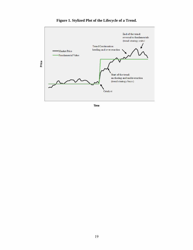
The economic rationale underlying trend-following strategies is illustrated in Figure

1, a stylized “lifecycle” of a trend. An initial under-reaction to a shift in fundamental

value allows a trend-following strategy to invest before new information is fully reflected

in prices. The trend then extends beyond fundamentals due to herding effects, and finally

results in a reversal. We discuss the drivers of each phase of this stylized trend, as well as

the related literature.

Start of the Trend: Under-Reaction to Information.

In the stylized example shown in Figure 1, a catalyst – a positive earnings release, a

supply shock, or a demand shift – causes the value of an equity, commodity, currency, or

bond to change. The change in value is immediate, shown by the solid blue line. While

the market price (shown by the dotted black line) moves up as a result of the catalyst, it

initially under-reacts and therefore continues to go up for a while. A trend-following

strategy buys the asset as a result of the initial upward price move, and therefore

capitalizes on the subsequent price increases. At this point in the lifecycle, trend-

following investors contribute to the speeding-up of the price discovery process.

Research has documented a number of behavioral tendencies and market frictions that

lead to this initial under-reaction:

i. Anchor-and-insufficient-adjustment. Edwards (1968), and Tversky and

Kahneman (1974) find that people anchor their views to historical data and

adjust their views insufficiently to new information. This behavior can cause

prices to under-react to news (Barberis, Shleifer, and Vishny (1998)).

ii. The disposition effect. Shefrin and Statman (1985), and Frazzini (2006)

observe that people tend to sell winners too early and ride losers too long.

They sell winners early because they like to realize their gains. This creates

downward price pressure, which slows the upward price adjustment to new

positive information. On the other hand, people hang on to losers because

6

realizing losses is painful. They try to “make back” what has been lost. Fewer

willing sellers can keep prices from adjusting downward as fast as they

should.

iii. Non-profit-seeking activities. Central banks operate in the currency and

fixed-income markets to reduce exchange-rate and interest-rate volatility,

potentially slowing the price-adjustment to news (Silber (1994)). Also,

investors who mechanically rebalance to strategic asset allocation weights

trade against trends. For example, a 60/40 investor who seeks to own 60%

stocks and 40% bonds will sell stocks (and buy bonds) whenever stocks have

outperformed.

iv. Frictions and slow moving capital. Frictions, delayed response by some

market participants, and slow moving arbitrage capital can also slow price

discovery and lead to a drop and rebound of prices (Mitchell, Pedersen, and

Pulvino (2007), Duffie (2010)).

The combined effect is for the price to move too gradually in response to news,

creating a price drift as the market price slowly incorporates the full effect of the news. A

trend-following strategy will position itself in relation to the initial news, and profit if the

trend continues.

Trend Continuation: Delayed Over-Reaction

Once a trend has started, a number of other phenomena exist which may extend the

trend beyond the fundamental value:

i. Herding and feedback trading. When prices have moved in one direction for

a while, some traders may jump on the bandwagon because of herding

(Bikhchandani et al. (1992)) or feedback trading (De Long et al. (1990), Hong

and Stein (1999)). Herding has been documented among equity analysts in

their recommendations and earnings forecasts (Welch (2000)), in investment

newsletters (Graham (1999)), and in institutional investment decisions.

ii. Confirmation bias and representativeness. Wason (1960) and Tversky and

Kahneman (1974) show that people tend to look for information that confirms

what they already believe, and look at recent price moves as representative of

7

the future. This can lead investors to move capital into investments that have

recently made money, and conversely out of investments that have declined,

both of which cause trends to continue (Barberis, Shleifer, and Vishny (1998),

Daniel, Hirshleifer, Subrahmanyam (1998)).

iii. Fund flows and risk management. Fund flows often chase recent

performance (perhaps because of i. and ii.). As investors pull money from

underperforming managers, these managers respond by reducing their

positions (which have been underperforming), while outperforming managers

receive inflows, adding buying pressure to their outperforming positions.

Further, some risk-management schemes imply selling in down-markets and

buying in up-markets, in line with the trend. Examples of this behavior

include stop-loss orders, portfolio insurance, and corporate hedging activity

(e.g., an airline company that buys oil futures after the oil price has risen to

protect the profit margins from falling too much, or a multinational company

that hedges foreign-exchange exposure after a currency moved against it).

End of the Trend

Obviously, trends cannot go on forever. At some point, prices extend too far beyond

fundamental value and, as people recognize this, prices revert towards the fundamental

value and the trend dies out. As evidence of such over-extended trends, Moskowitz, Ooi,

and Pedersen (2012) find evidence of return reversal after more than a year.3 The return

reversal only reverses part of the initial price trend, suggesting that the price trend was

partly driven by initial under-reaction (since this part of the trend should not reverse) and

partly driven by delayed over-reaction (since this part reverses).

3. TimeSeriesMomentumAcrossTrend‐HorizonsandMarkets

Having discussed why trends might exist, we now demonstrate the performance of a

simple trend-following strategy: time series momentum.

Identifying Trends and Sizing Positions

3 Such long-run reversal is also found in the cross-section of equities (De Bondt and Thaler (1985)) and the cross-section of global asset classes (Asness, Moskowitz, and Pedersen (2012)).

8

We construct time series momentum strategies for 58 highly liquid futures and

currency forwards from January 1985 to June 2012 – specifically 24 commodity futures,

9 equity index futures, 13 bond futures, and 12 currency forwards. To determine the

direction of the trend in each asset, the strategy simply considers whether the asset’s

excess return is positive or negative: A positive past return is considered an “up trend,”

and leads to a long position; a negative return is considered a “down trend,” and leads to

a short position.

We consider 1-month, 3-month, and 12-month time series momentum strategies,

corresponding to short-, medium-, and long-term trend-following strategies. The 1-month

strategy goes long if the preceding 1-month excess return was positive, and short if it was

negative. The 3-month and 12-month strategies are constructed analogously. Hence, each

strategy always holds a long or a short position in each of 58 markets.

The size of each position is chosen to target an annualized volatility of 40% for that

asset, following the methodology of Moskowitz, Ooi, and Pedersen (2012).4 Specifically,

the number of dollars bought/sold of instrument s at time t is 40%/σ so that the time

series momentum (TSMOM) strategy realizes the following return during the next week:

, sign excess return of s over past X months% s

(1)

The ex-ante annualized volatility for each instrument is estimated as an exponentially

weighted average of past squared returns

261∑ 1 s ̅s (2)

where the scalar 261 scales the variance to be annual and ̅s is the exponentially weighted

average return computed similarly. The parameter δ is chosen so that the center of mass

of the weights, given by ∑ 1 , is equal to 60 days.

4 Our position sizes are chosen to target a constant volatility for each instrument, but, more generally, one could consider strategies that vary the size of the position based on the strength of the estimated trend. E.g., for intermediate price moves, one could take a small position or no position and increase the position depending on the magnitude of the price move. However, the goal of our paper is not to determine the optimal trend-following strategy, but to show that even a simple approach performs well and can explain the returns in the CTA industry.

9

This constant-volatility position-sizing methodology of Moskowitz, Ooi, and

Pedersen (2012) is useful for several reasons: First, it enables us to aggregate the

different assets into a diversified portfolio which is not overly dependent on the riskier

assets – this is important given the large dispersion in volatility among the assets we

trade. Second, this methodology keeps the risk of each asset stable over time, so that the

strategy’s performance is not overly dependent on what happens during times of high

risk. Third, the methodology minimizes the risk of data mining given that it does not use

any free parameters or optimization in choosing the position sizes.

The portfolio is rebalanced weekly at the closing price each Friday, based on data

known at the end of each Thursday. We therefore are only using information available at

the time to make the strategies implementable. The strategy returns are gross of

transaction costs, but we note that the instruments we consider are among the most liquid

in the world. Sections 5 considers the effect of different rebalance rules and discusses the

impact of transaction costs. While Moskowitz, Ooi, and Pedersen (2012) focus on

monthly rebalancing, it is interesting to also consider higher rebalancing frequencies

given our focus on explaining the returns of professional money managers who often

trade throughout the day.

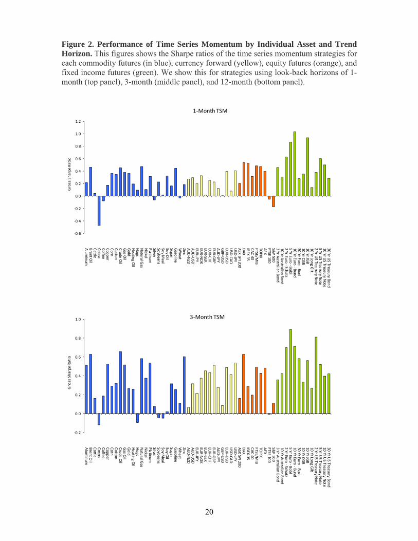
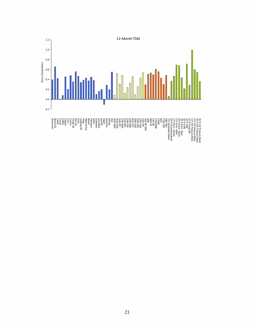
Performance of the TSMOM Strategies by Individual Asset

Figure 2 shows the performance of each time series momentum strategy in each asset.

The strategies deliver positive results in almost every case, a remarkably consistent result.

The average Sharpe Ratio (excess returns divided by realized volatility) across assets is

0.29 for the 1-month strategy, 0.36 for the 3-month strategy, and 0.38 for the 12-month

strategy.

Building Diversified TSMOM Strategies

Next, we construct diversified 1-month, 3-month, and 12-month time series

momentum strategies by averaging returns of all the individual strategies that share the

same look-back horizon (denoted, , and ). We also

construct time series momentum strategies for each of the four asset classes:

commodities, currencies, equities, and fixed income

(denoted, , , , ). E.g., the commodity

10

strategy is the average return of each individual commodity strategy for all 3 trend

horizons. Finally, we construct a strategy that diversifies across all assets and all trend

horizons that we call the diversified time series momentum strategy (denoted simply,

TSMOM). In each case, we scale the positions to target an ex ante volatility of 10% using

an exponentially-weighted variance-covariance matrix estimated analogously to Equation

(2).

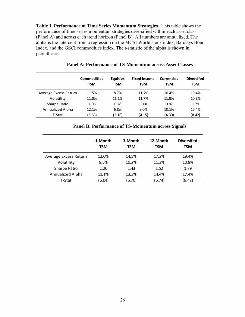
Table 1 shows the performance of these diversified time series momentum strategies.

We see that the strategies’ realized volatilities closely match the 10% ex ante target,

varying from 9.5% to 11.9%. More importantly, all the time series momentum strategies

have impressive Sharpe ratios, reflecting a high average excess return above the risk-free

rate relative to the risk. Comparing the strategies across trend horizons, we see that the

long-term (12-month) strategy has performed the best, the medium-term strategy has

done second best, and the short-term strategy, which has the lowest Sharpe Ratio out of

the 3 strategies, still has a high Sharpe Ratio of 1.3. Comparing asset classes,

commodities, fixed income, and currencies have performed a little better than equities.

In addition to reporting the expected return, volatility, and Sharpe ratio, Table 1 also

shows the alpha from the following regression:

Stocks Bonds Commodities (3)

We regress the TSMOM strategies on the returns of a passive investment in the MSCI

world stock index, the Barclays US Aggregate Government Bond index and the S&P

GSCI commodity index. The alpha measures the excess return, controlling for the risk

premia associated with simply being long these traditional asset classes. The alphas are

almost as large as the excess returns since the TSMOM strategies are long/short and

therefore have small average loadings on these passive factors. Finally, Table 1 reports

the t-statistics of the alphas, which show that the alphas are highly statistically

significant.

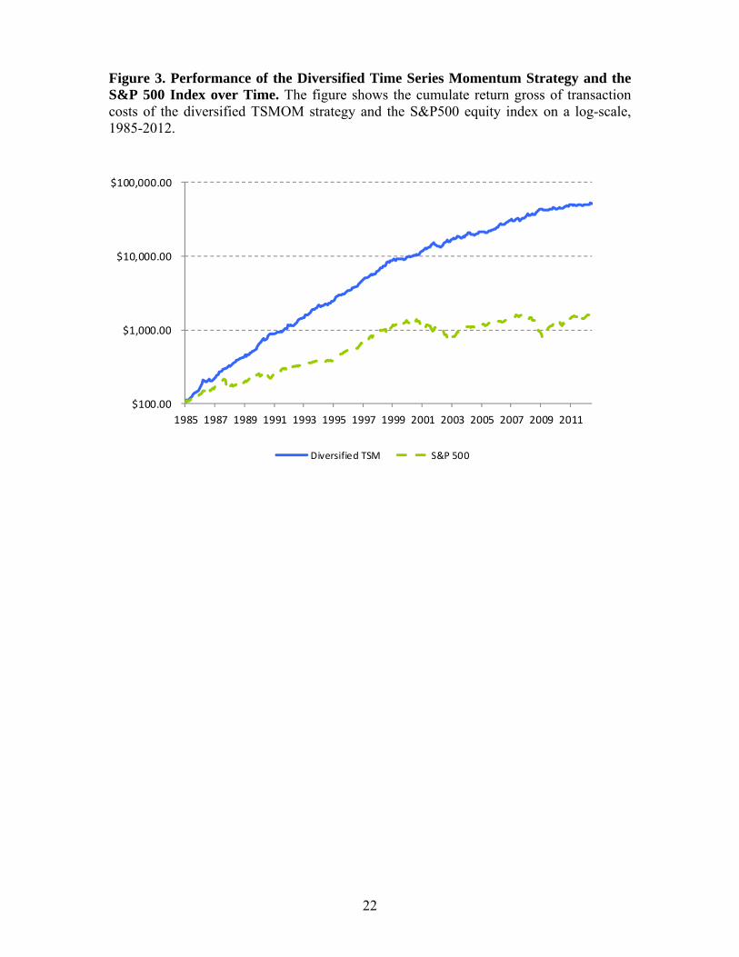
The best performing strategy is the diversified time series momentum strategy with a

Sharpe ratio of 1.8. Its consistent cumulative return is seen in Figure 3 that illustrates the

hypothetical growth of $100 invested in 1985 in the diversified TSMOM strategy and the

S&P500 stock market index, respectively.

11

Diversification: Trends with Benefits

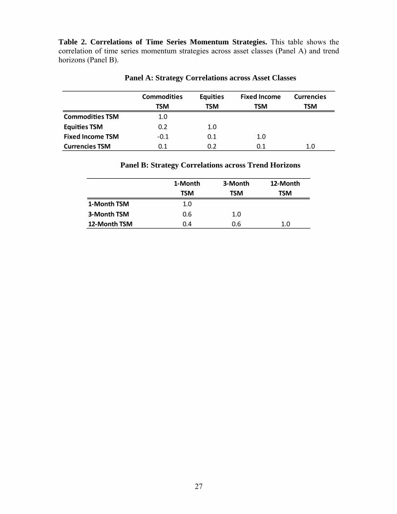
To understand this strong performance of time series momentum, note first that the

average pair-wise correlation of these single-asset strategies is less than 0.1 for each trend

horizon, meaning that the strategies behave rather independently across markets so one

may profit when another loses. Even when the strategies are grouped by asset class or

trend horizon, these relatively diversified strategies also have modest correlations as seen

in Table 2. Another reason for the strong benefits of diversification is our equal-risk

approach. The fact that we scale our positions so that each asset has the same ex ante

volatility at each time means that, the higher the volatility of an asset, the smaller a

position it has in the portfolio, creating a stable and risk-balanced portfolio. This is

important because of the wide range of volatilities exhibited across assets. For example, a

5-year US government bond future typically exhibits a volatility of around 5% a year,

while a natural gas future typically exhibits a volatility of around 50% a year. If a

portfolio holds the same notional exposure to each asset in the portfolio (as some indices

and managers do), the risk and returns of the portfolio will be dominated by the most

volatile assets, significantly reducing the diversification benefits.

The diversified time series momentum strategy has very low correlations to

traditional asset classes. Indeed, the correlation with the S&P500 stock market index is -

0.02, the correlation with the bond market as represented by the Barclays US Aggregate

index is 0.23, and the correlation with the S&P GSCI commodity index is 0.05. Further,

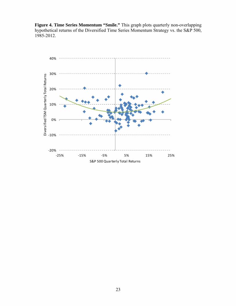
the time series momentum strategy has performed especially well during periods of

prolonged bear markets and in sustained bull markets as seen in Figure 4. Figure 4 plots

the quarterly returns of time series momentum against the quarterly returns of the

S&P500. We estimate a quadratic function to fit the relation between time series

momentum returns and market returns, giving rise to a “smile” curve. The estimated

smile curve means that time series momentum has historically done the best during

significant bear markets or significant bull markets, performing less well in flat markets.

To understand this smile effect, note that most of the worst equity bear markets have

historically happened gradually. The market first goes from “normal” to “bad”, causing a

TSMOM strategy to go short (while incurring a loss or profit depending on what

happened previously). Often, a deep bear market happens when the market goes from

“bad” to “worse”, traders panic and prices collapse. This leads to profits on the short

12

positions, explaining why these strategies tend to be profitable during such extreme

events. Of course, these strategies will not always profit during extreme events. For

instance, the strategy might incur losses if, after a bull market (which would get the

strategy positioned long), the market crashed quickly before the strategy could alter its

positions to benefit from the crash.

4. TimeSeriesMomentumExplainsActualManagedFuturesFundReturns

We collect the returns of two major Managed Futures indices, BTOP 50 and DJCS

Managed Futures Index,5 as well as individual fund returns from the Lipper/Tass

database in the category labeled “Managed Futures.” We highlight the performance of the

5 Managed Futures funds in the Lipper/Tass database that have the largest reported

“Fund Assets” as of 06/2012. While looking at the ex post returns of the largest funds

naturally bias us toward picking funds that did well, it is nevertheless interesting to

compare these most successful funds to time series momentum.

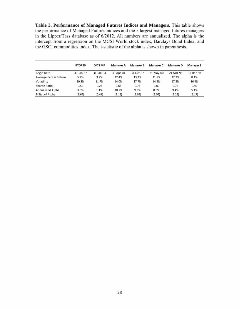
Table 3 reports the performance of the Managed Futures indices. We see that the

index and manager returns have Sharpe ratios between 0.27 and 0.88. All of the alphas

with respect to passive exposures to stocks/bonds/commodities are positive and most of

them are statistically significant. We see that the diversified time series momentum

strategy has a higher Sharpe ratio and alpha than the indices and managers, but we note

that time series momentum index is gross of fees and transaction costs while the

managers and indices are after fees and transaction costs. Further, while the time series

momentum strategy is simple and subject to minimal data-mining, it does benefit from

some hindsight in choosing its 1, 3, and 12-month trend horizons – managers

experiencing losses in real time may have had a more difficult time sticking with these

strategies through tough times than our hypothetical strategy.

Fees make a significant difference given that most CTAs and Managed Futures hedge

funds have historically charged at least 2% management fees and 20% performance fees.

While we cannot know the exact before-fee manager returns, we can simulate the

5 These index returns are available at the following websites: http://www.barclayhedge.com/research/indices/btop/index.html http://www.hedgeindex.com/hedgeindex/secure/en/indexperformance.aspx?cy=USD&indexname=HEDG_MGFUT

13

hypothetical fee for the time series momentum strategy. With a 2-and-20 fee structure,

the average fee is around 6% per year for the diversified TSMOM strategy.6 We calculate

this average fee using a 2-and-20 fee structure, high water marks, quarterly payments of

management fees, and annual payments of performance fees. Further, transaction costs

are on the order of 1-4% per year for a sophisticated manager and possibly much higher

for less sophisticated managers and higher historically.7 Hence, after these estimated fees

and transaction costs, the Sharpe ratio of the diversified time series momentum strategy

would historically have been near 1, still comparing well to the indices and managers, but

we note that historical transaction costs are not known and associated with significant

uncertainty.

Rather than comparing the performance of the time series momentum strategy to

those of the indices and managers, we want to show that time series momentum can

explain the strong performance of Managed Futures managers. To explain Managed

Futures returns, we regress the returns of Managed Futures indices and managers ( MF)

on the returns of 1-month, 3-month, and 12-month time series momentum:

MF (4)

Similarly, we regress the returns of Managed Futures indices and managers on the

returns of TSMOM strategies in commodities ( ), equities ( ), fixed

income ( ), and currencies ( ):

MF

(5)

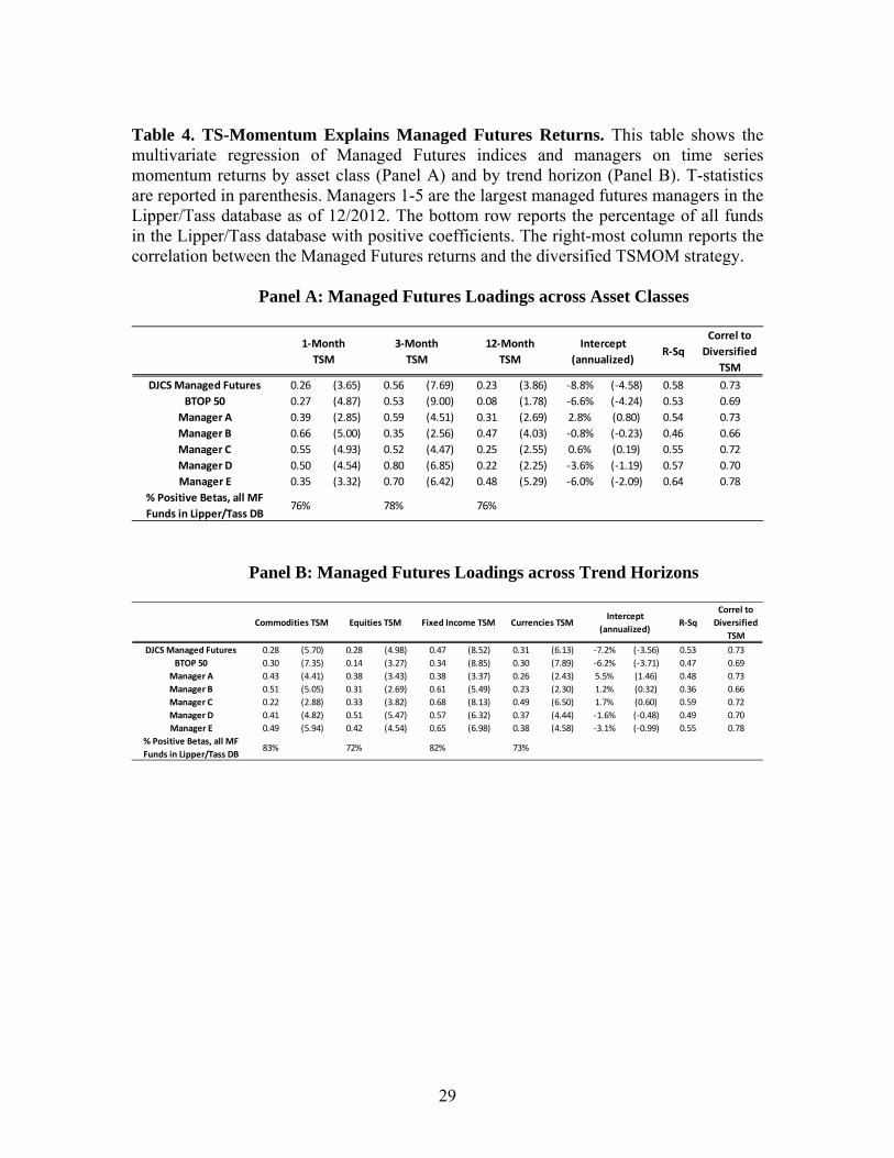
Table 4 reports the results of these regressions. We see the time series momentum

strategies explain the Managed Futures index and manager returns to a large extent in the

sense that the R-squares of these regressions are large, ranging between 0.36 and 0.64.

6 The average fee is high due to the high Sharpe Ratio realized by the simulated TSMOM strategy. In practice, Managed Futures indices have realized lower Sharpe Ratios. 7 This estimate of transaction costs is based on proprietary estimates of current transaction costs in global futures and forward markets combined with the turnover of these strategies for a manager with about USD1 Billion under management. These estimates do not account for the fact that transaction costs were higher in earlier years when markets were less liquid and trading was not conducted via electronic markets.

14

Table 4 also reports the correlation of the Managed Futures indices and managers with

the diversified TSMOM strategy. These correlations are large, ranging from 0.66 to 0.78,

which provides another indication that time series momentum can explain the Managed

Futures universe.

The intercepts reported in Table 4 indicate the excess returns (or alphas) after

controlling for time series momentum. While the alphas relative to the traditional asset

classes in Table 3 were significantly positive, almost all the alphas relative to time series

momentum in Table 4 are negative. Even though the returns of the largest managers are

biased be to be high (due to the ex post selection of the managers), time series

momentum nevertheless drives these alphas to be negative. This is another expression

that time series momentum can explain the Managed Futures space and an illustration of

the importance of fees and transaction costs.

Another interesting finding that arises from Table 4 is the relative importance of

short-, medium-, and long-term trends for Managed Futures funds, as well as the relative

importance of the different asset classes. We see that all the indices and managers have

positive loadings on all the trend horizons and all the asset classes, and almost all the

loadings are statistically significant. Focusing on the DJCS Managed Futures index,

Figure 5 illustrates the relative loadings on the different trend horizons and the different

asset classes. As seen in Table 4 and Figure 5, most managers put most weight on

medium- and long-term trends, with less weight on short-term trends. In terms of asset

classes, most managers put more weight on fixed income, perhaps because of the

liquidity of these markets and the strong performance of fixed income trend following in

the past decades.

In summary, while many Managed Futures funds pursue many other types of

strategies besides time series momentum, such as carry strategies and global macro

strategies, our results show that time series momentum explains the average alpha in the

industry and a significant fraction of the time-variation of returns.

5. Implementation:HowtoManageManagedFutures

We have seen that time series momentum can explain Managed Futures returns. In

fact, this relatively simple strategy has realized a higher Sharpe ratio than most managers,

at least on paper. This suggests that fees and other implementation issues are important

15

for the real-world success of these strategies. Indeed, as mentioned in Section 4, we

estimate that a 2-20 fee structure implies a 6% average annual fee on the diversified time

series momentum strategy run at a 10% annualized volatility. Other important

implementation issues include transaction costs, rebalance methodology, margin

requirements, and risk management.

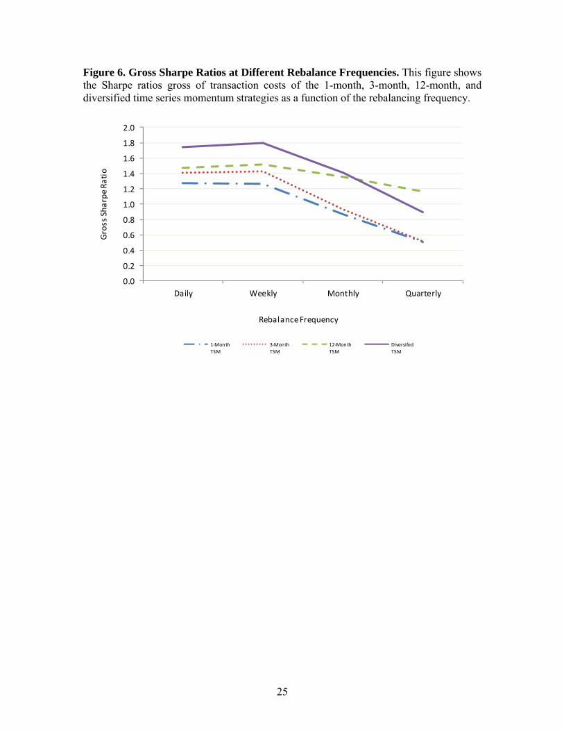
To analyze the effect of how often the portfolio is rebalanced, Figure 6 shows the

gross Sharpe ratio for each trend horizon and the diversified time series momentum

strategy as a function of rebalancing frequency. Daily and weekly rebalancing perform

similarly, while the performance trails off with monthly and quarterly rebalancing

frequencies. Naturally, the performance falls more quickly for the short and medium-term

strategies as these signals change more quickly, leading to a larger alpha decay.

As mentioned, the annual transaction costs of a Managed Futures strategy are

typically about 1-4% for a sophisticated trader, possibly much higher for less

sophisticated traders, and higher historically given higher transactions costs in the past.

Transaction costs depend on a number of things. Transaction costs increase with

rebalance frequency if the portfolio is mechanically rebalanced without transaction-cost

optimization, although more frequent access to the market can also be used to source

more liquidity. Garleanu and Pedersen (2012) derive an optimal portfolio rebalancing

rule for many assets with several returns predictors (such as trend signals) and transaction

costs. They find that transaction cost optimization leads to a larger optimal weight on

signals with slower alpha decay, that is, longer-term trends. Hence, larger managers may

allocate a larger weight to medium- and long-term trend signals and relatively lower

weight to short-term signals, as seen in Figure 5B. Transaction costs rise with the weight

given to more illiquid assets, and rise with the size of the fund for a given trading

infrastructure, although large funds should have the ability to develop better trading

infrastructure and negotiate lower commissions. Transaction costs are lower for managers

who have more direct market access (saving on commissions and indirect broker costs)

with advanced trading algorithms that can partly provide liquidity and have minimal

information leakage.

To implement managed futures strategies, managers must post margin to

counterparties, namely the Futures Commission Merchant and the currency

intermediation agent (or currency prime broker). The time series momentum strategy

would typically have margin requirements of 8-12% for a large institutional investor, and

16

more than double that for a smaller investor. Hence, time series momentum is certainly

implementable from a funding liquidity standpoint as it has a significant amount of free

cash.

Risk management is the final implementation issue that we discuss. Our construction

of trading strategies is systematic and already has built-in risk controls due to our

constant-volatility methodology. This methodology is important for several reasons. First,

it controls the risk of each security by scaling down the position when risk spikes up.

Second, it achieves a risk-balanced diversification across securities at all times. Third,

our systematic implementation means that our strategies are not subject to behavioral

biases. Moreover, our methodology can be overlaid with an additional layer of risk

management and drawdown control and some Managed Futures managers further seek to

identify over-extended trends to limit the losses from sharp trend-reversals, and try to

identify short-term countertrends to improve performance in range-bound markets.

6. Conclusion

We find that 1-month, 3-month, and 12-month time series momentum strategies have

performed well over time and across asset classes. Combining these into a diversified

time series momentum strategy produces a gross Sharpe ratio of 1.8, performing well in

both in extended bear and bull markets. Time series momentum can explain Managed

Futures indices and manager returns, even for the ex-post largest and most successful

funds, demystifying the strategy. Indeed, time series momentum has a high correlation to

Managed Futures returns, large R-squares, and explains the average returns (that is,

leaves only a small unexplained intercept or alpha in a regression). Thus investors can get

exposure to Managed Futures using time series momentum strategies, and should pay

attention to implementation issues such as fees, trading infrastructure and risk

management procedures used by different managers.

17

References

Asness, C. (1994), “Variables that Explain Stock Returns.” Ph.D. Dissertation, University of Chicago. Asness, C., T.J. Moskowitz, and L.H. Pedersen, (2009) “Value and Momentum Everywhere,” National Bureau of Economic Research. Baltas, A.-N. and R. Kosowski (2013), “Momentum Strategies in Futures Markets and Trend-following Funds,” working paper, Imperial College. Barberis, N. A. Shleifer and R. Vishny (1998), “A Model of Investor Sentiment,” Journal of Financial Economics 49, 307-343. Bikhchandani, S., D. Hirshleifer, and I. Welch (1992), “A theory of fads, fashion, custom, and cultural change as informational cascades,” Journal of political Economy, 100, 5, 992-1026. Chabot, B., E. Ghysels, and R. Jagannathan (2009), “Momentum Cycles and Limits to Arbitrage: Evidence from Victorian England and Post-Depression US Stock Markets,” working paper, Yale University. Cutler, D.M., Poterba, J.M., and Summers, L.H. (1991), “Speculative dynamics,” Review of Economic Studies 58, 529–546. Daniel, K., D. Hirshleifer, A. Subrahmanyam (1998), “A theory of overconfidence, self-attribution, and security market under- and over-reactions,” Journal of Finance 53, 1839-1885. De Bondt, W. F. M. and R. Thaler (1985), “Does the Stock Market Overreact?,” The Journal of Finance 40(3), 793-805. De Long, J.B., A. Shleifer, L. H. Summers, and Waldmann, R.J. (1990), “Positive feedback investment strategies and destabilizing rational speculation,” The Journal of Finance, 45, 2, 379-395. Duffie, D. (2010), “Asset Price Dynamics with Slow-Moving Capital,” Journal of Finance 2010, 65, 1238-1268. Edwards, W.,(1968), “Conservatism in human information processing,” In: Kleinmutz, B. (Ed.), Formal Representation of Human Judgment. John Wiley and Sons, New York, pp. 17-52. Elton, E. J. and M. J. Gruber, and J. C. Rentzler (1987), “Professionally Managed, Publicly Traded Commodity Funds,” The Journal of Business, vol. 60, no. 2, 175-199

18

Frazzini, A. (2006), “The Disposition Effect and Underreaction to News.” Journal of Finance, 61. Fung, W., and D. Hsieh (2001), “The risk in hedge fund strategies: theory and evidence from trend followers,” Review of Financial Studies 14, 313–341. Garleanu, N. and L.H. Pedersen (2007), “Liquidity and Risk Management,” The American Economic Review, 97, 193-197. Garleanu, N. and L.H. Pedersen (2012), “Dynamic Trading with Predictable Returns and Transaction Costs,” Journal of Finance, forthcoming. Graham, J.R. (1999), “Herding Among Investment Newsletters: Theory and Evidence,” Journal of Finance 54:1, 237-268. Hong, H. and J. Stein (1999), “A Unified Theory of Underreaction, Momentum Trading and Overreaction in Asset Markets,” Journal of Finance, LIV, no. 6. Jegadeesh, N. and S. Titman (1993), “Returns to buying winners and selling losers: Implications for stock market efficiency,” Journal of Finance 48, 65–91. Mitchell, M., L.H. Pedersen, and T. Pulvino (2007), “Slow Moving Capital,” The American Economic Review, 97, 215-220. Moskowitz, T., Y.H. Ooi, and L.H. Pedersen (2012), “Time series momentum,” Journal of Financial Economics 104(2), 228-250. Shefrin, H., and M. Statman (1985), “The disposition to sell winners too early and ride losers too long: Theory and evidence,” Journal of Finance 40, 777–791. Silber, W.L. (1994), “Technical trading: when it works and when it doesn't,” Journal of Derivatives, vol 1, no. 3, 39-44. Tversky, A. and D. Kahneman (1974), “Judgment under uncertainty: heuristics and biases,” Science 185, 1124-1131. Wason, P.C. (1960), “On the failure to eliminate hypotheses in a conceptual task,” The Quarterly Journal of Experimental Psychology, 12, 129-140. Welch, I. (2000), “Herding among security analysts,” Journal of Financial Economics 58, 69–396.

19

Figure 1. Stylized Plot of the Lifecycle of a Trend.

20

Figure 2. Performance of Time Series Momentum by Individual Asset and Trend Horizon. This figures shows the Sharpe ratios of the time series momentum strategies for each commodity futures (in blue), currency forward (yellow), equity futures (orange), and fixed income futures (green). We show this for strategies using look-back horizons of 1-month (top panel), 3-month (middle panel), and 12-month (bottom panel).

‐0.6

‐0.4

‐0.2

0.0

0.2

0.4

0.6

0.8

1.0

1.2

Aluminum

Brent O

ilCattle

Cocoa

Coffee

Copper

Corn

Cotto

nCrude

 Oil

Gas O

ilGold

Heatin

g Oil

Hogs

Natu

ral Gas

Nickel

Platinu

mSilve

rSoybean

sSoy M

ealSoy O

ilSuga

rGaso

lineWheat

ZincAUD‐NZD

AUD‐USD

EUR‐JP

YEU

R‐NOK

EUR‐SEK

EUR‐CHF

EUR‐GBP

AUD‐JP

YGBP‐U

SDEU

R‐USD

USD

‐CAD

USD

‐JPYASX

 SPI 20

0DAX

IBEX

 35CAC 40

FTSE/MIB

TOPIX

AEX

FTSE 100

S&P 50

03 Yr A

ustralian

 Bond

10 Yr A

ustralian B

ond

2 Yr Euro ‐ Sch

atz5 Yr Eu

ro ‐ B

obl

10 Yr Eu

ro ‐ B

und

30 Yr Eu

ro ‐ B

uxl10

 Yr CGB

10 Yr JG

B10

 Yr Long G

ilt2 Yr U

S Treasury N

ote

5 Yr US Trea

sury N

ote

10 Yr U

S Treasury N

ote30

 Yr US Treasu

ry Bond

Gross Sharpe Ratio 

1‐Month TSM

‐0.2

0.0

0.2

0.4

0.6

0.8

1.0

Aluminum

Brent O

ilCattle

Cocoa

Coffee

Copper

Corn

Cotto

nCrude

 Oil

Gas O

ilGold

Heatin

g Oil

Hogs

Natu

ral Gas

Nickel

Platinu

mSilve

rSoybean

sSoy M

ealSoy O

ilSuga

rGaso

lineWheat

ZincAUD‐NZD

AUD‐USD

EUR‐JP

YEU

R‐NOK

EUR‐SEK

EUR‐CHF

EUR‐GBP

AUD‐JP

YGBP‐U

SDEU

R‐USD

USD

‐CAD

USD

‐JPYASX

 SPI 20

0DAX

IBEX

 35CAC 40

FTSE/MIB

TOPIX

AEX

FTSE 100

S&P 50

03 Yr A

ustralian

 Bond

10 Yr A

ustralian B

ond

2 Yr Euro ‐ Sch

atz5 Yr Eu

ro ‐ B

obl

10 Yr Eu

ro ‐ B

und

30 Yr Eu

ro ‐ B

uxl10

 Yr CGB

10 Yr JG

B10

 Yr Long G

ilt2 Yr U

S Treasury N

ote

5 Yr US Trea

sury N

ote

10 Yr U

S Treasury N

ote30

 Yr US Treasu

ry Bond

Gross Sharpe Ratio 

3‐Month TSM

21

‐0.2

0.0

0.2

0.4

0.6

0.8

1.0

1.2

Aluminum

Brent O

ilCattle

Cocoa

Coffee

Copper

Corn

Cotto

nCrude

 Oil

Gas O

ilGold

Heatin

g Oil

Hogs

Natu

ral Gas

Nickel

Platinu

mSilve

rSoybean

sSoy M

ealSoy O

ilSuga

rGaso

lineWheat

ZincAUD‐NZD

AUD‐USD

EUR‐JP

YEU

R‐NOK

EUR‐SEK

EUR‐CHF

EUR‐GBP

AUD‐JP

YGBP‐U

SDEU

R‐USD

USD

‐CAD

USD

‐JPYASX

 SPI 20

0DAX

IBEX

 35CAC 40

FTSE/MIB

TOPIX

AEX

FTSE 100

S&P 50

03 Yr A

ustralian

 Bond

10 Yr A

ustralian B

ond

2 Yr Euro ‐ Sch

atz5 Yr Eu

ro ‐ B

obl

10 Yr Eu

ro ‐ B

und

30 Yr Eu

ro ‐ B

uxl10

 Yr CGB

10 Yr JG

B10

 Yr Long G

ilt2 Yr U

S Treasury N

ote

5 Yr US Trea

sury N

ote

10 Yr U

S Treasury N

ote30

 Yr US Treasu

ry Bond

Gross Sharpe Ratio 

12‐Month TSM

22

Figure 3. Performance of the Diversified Time Series Momentum Strategy and the S&P 500 Index over Time. The figure shows the cumulate return gross of transaction costs of the diversified TSMOM strategy and the S&P500 equity index on a log-scale, 1985-2012.

$100.00

$1,000.00

$10,000.00

$100,000.00

1985 1987 1989 1991 1993 1995 1997 1999 2001 2003 2005 2007 2009 2011

Diversified TSM S&P 500

23

Figure 4. Time Series Momentum “Smile.” This graph plots quarterly non-overlapping hypothetical returns of the Diversified Time Series Momentum Strategy vs. the S&P 500, 1985-2012.

‐20%

‐10%

0%

10%

20%

30%

40%

‐25% ‐15% ‐5% 5% 15% 25%

Diversified

 TSM

 Quarterly Total Returns

S&P 500 Quarterly Total  Returns

24

Figure 5. Managed Futures Exposures across Asset Classes and Trend Horizons. This figure shows the regression coefficients from a regression of the DJCS Managed Futures Index on the time series momentum strategies by asset class (Panel A) and by trend horizon. The regression coefficients are scaled by their sum to show their relative importance.

Panel A: Exposures across Asset Classes

Panel B: Exposures across Trend Horizons

Commodities TSM,  21%

Equities TSM,  21%

Fixed Income TSM,  35%

Currencies TSM,  23%

1‐Month TSM,  24%

3‐Month TSM,  54%

12‐Month TSM,  22%

25

Figure 6. Gross Sharpe Ratios at Different Rebalance Frequencies. This figure shows the Sharpe ratios gross of transaction costs of the 1-month, 3-month, 12-month, and diversified time series momentum strategies as a function of the rebalancing frequency.

0.0

0.2

0.4

0.6

0.8

1.0

1.2

1.4

1.6

1.8

2.0

Daily Weekly Monthly Quarterly

Gross Sharpe Ratio

Rebalance Frequency

1‐MonthTSM

3‐MonthTSM

12‐MonthTSM

DiversifedTSM

26

Table 1. Performance of Time Series Momentum Strategies. This table shows the performance of time series momentum strategies diversified within each asset class (Panel A) and across each trend horizon (Panel B). All numbers are annualized. The alpha is the intercept from a regression on the MCSI World stock index, Barclays Bond Index, and the GSCI commodities index. The t-statistic of the alpha is shown in parentheses.

Panel A: Performance of TS-Momentum across Asset Classes

Panel B: Performance of TS-Momentum across Signals

Commodities 

TSM

Equities 

TSM

Fixed Income 

TSM

Currencies 

TSM

Diversifed 

TSM

Average Excess Return 11.5% 8.7% 11.7% 10.4% 19.4%

Volatility 11.0% 11.1% 11.7% 11.9% 10.8%

Sharpe Ratio 1.05 0.78 1.00 0.87 1.79

Annualized Alpha 12.1% 6.8% 9.0% 10.1% 17.4%

T‐Stat (5.63) (3.16) (4.15) (4.30) (8.42)

1‐Month 

TSM

3‐Month 

TSM

12‐Month 

TSM

Diversifed 

TSM

Average Excess Return 12.0% 14.5% 17.2% 19.4%

Volatility 9.5% 10.2% 11.3% 10.8%

Sharpe Ratio 1.26 1.43 1.52 1.79

Annualized Alpha 11.1% 13.3% 14.4% 17.4%

T‐Stat (6.04) (6.70) (6.74) (8.42)

27

Table 2. Correlations of Time Series Momentum Strategies. This table shows the correlation of time series momentum strategies across asset classes (Panel A) and trend horizons (Panel B).

Panel A: Strategy Correlations across Asset Classes

Panel B: Strategy Correlations across Trend Horizons

Commodities 

TSM

Equities 

TSM

Fixed Income 

TSM

Currencies 

TSM

Commodi es TSM 1.0

Equi es TSM 0.2 1.0

Fixed Income TSM ‐0.1 0.1 1.0

Currencies TSM 0.1 0.2 0.1 1.0

1‐Month 

TSM

3‐Month 

TSM

12‐Month 

TSM

1‐Month TSM 1.0

3‐Month TSM 0.6 1.0

12‐Month TSM 0.4 0.6 1.0

28

Table 3. Performance of Managed Futures Indices and Managers. This table shows the performance of Managed Futures indices and the 5 largest managed futures managers in the Lipper/Tass database as of 6/2012. All numbers are annualized. The alpha is the intercept from a regression on the MCSI World stock index, Barclays Bond Index, and the GSCI commodities index. The t-statistic of the alpha is shown in parenthesis.

BTOP50 DJCS MF Manager A Manager B Manager C Manager D Manager E

Begin Date 30‐Jan‐87 31‐Jan‐94 30‐Apr‐04 31‐Oct‐97 31‐May‐00 29‐Mar‐96 31‐Dec‐98

Average Excess Return 5.2% 3.2% 12.4% 13.3% 11.8% 12.3% 8.1%

Volatility 10.3% 11.7% 14.0% 17.7% 14.8% 17.2% 16.4%

Sharpe Ratio 0.50 0.27 0.88 0.75 0.80 0.72 0.49

Annualized Alpha 3.5% 1.1% 10.7% 9.3% 8.5% 9.4% 5.1%

T‐Stat of Alpha (1.69) (0.41) (2.15) (2.05) (2.05) (2.22) (1.17)

29

Table 4. TS-Momentum Explains Managed Futures Returns. This table shows the multivariate regression of Managed Futures indices and managers on time series momentum returns by asset class (Panel A) and by trend horizon (Panel B). T-statistics are reported in parenthesis. Managers 1-5 are the largest managed futures managers in the Lipper/Tass database as of 12/2012. The bottom row reports the percentage of all funds in the Lipper/Tass database with positive coefficients. The right-most column reports the correlation between the Managed Futures returns and the diversified TSMOM strategy.

Panel A: Managed Futures Loadings across Asset Classes

Panel B: Managed Futures Loadings across Trend Horizons

R‐Sq

Correl to 

Diversified 

TSM

DJCS Managed Futures 0.26 (3.65) 0.56 (7.69) 0.23 (3.86) ‐8.8% (‐4.58) 0.58 0.73

BTOP 50 0.27 (4.87) 0.53 (9.00) 0.08 (1.78) ‐6.6% (‐4.24) 0.53 0.69

Manager A 0.39 (2.85) 0.59 (4.51) 0.31 (2.69) 2.8% (0.80) 0.54 0.73

Manager B 0.66 (5.00) 0.35 (2.56) 0.47 (4.03) ‐0.8% (‐0.23) 0.46 0.66

Manager C 0.55 (4.93) 0.52 (4.47) 0.25 (2.55) 0.6% (0.19) 0.55 0.72

Manager D 0.50 (4.54) 0.80 (6.85) 0.22 (2.25) ‐3.6% (‐1.19) 0.57 0.70

Manager E 0.35 (3.32) 0.70 (6.42) 0.48 (5.29) ‐6.0% (‐2.09) 0.64 0.78

% Positive Betas, all MF 

Funds in Lipper/Tass DB76% 78% 76%

1‐Month 

TSM

3‐Month 

TSM

12‐Month 

TSM

Intercept 

(annualized)

R‐Sq

Correl to 

Diversified 

TSM

DJCS Managed Futures 0.28 (5.70) 0.28 (4.98) 0.47 (8.52) 0.31 (6.13) ‐7.2% (‐3.56) 0.53 0.73

BTOP 50 0.30 (7.35) 0.14 (3.27) 0.34 (8.85) 0.30 (7.89) ‐6.2% (‐3.71) 0.47 0.69

Manager A 0.43 (4.41) 0.38 (3.43) 0.38 (3.37) 0.26 (2.43) 5.5% (1.46) 0.48 0.73

Manager B 0.51 (5.05) 0.31 (2.69) 0.61 (5.49) 0.23 (2.30) 1.2% (0.32) 0.36 0.66

Manager C 0.22 (2.88) 0.33 (3.82) 0.68 (8.13) 0.49 (6.50) 1.7% (0.60) 0.59 0.72

Manager D 0.41 (4.82) 0.51 (5.47) 0.57 (6.32) 0.37 (4.44) ‐1.6% (‐0.48) 0.49 0.70

Manager E 0.49 (5.94) 0.42 (4.54) 0.65 (6.98) 0.38 (4.58) ‐3.1% (‐0.99) 0.55 0.78

% Positive Betas, all MF 

Funds in Lipper/Tass DB83% 72% 82% 73%

Fixed Income TSM Currencies TSMIntercept 

(annualized)Commodities TSM Equities TSM