Demonstration of a unified and flexible coupling environment for nonlinear fluid-

structure interaction problems

David THOMAS, Marco Lucio CERQUAGLIA, Romain BOMAN, Grigorios DIMITRIADIS, Vincent E. TERRAPON

Collaborative Conference on Physics Series CCPS 2018 – Fluid DynamicsSeptember 11-13, 2018, Barcelona, Spain

Department of Aerospace and Mechanical Engineering, University of Liège, Belgium

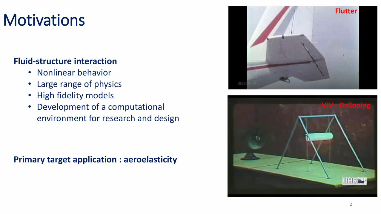
Motivations

2

Flutter

VIV - Galloping

Fluid-structure interaction• Nonlinear behavior• Large range of physics• High fidelity models• Development of a computational

environment for research and design

Primary target application : aeroelasticity

Computational approach

3

Monolithic• One single framework to solve the coupled problem

Partitioned• Coupling of independent codes• Each code is optimized for a particular physics

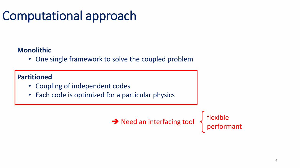
Computational approach

4

Monolithic• One single framework to solve the coupled problem

Partitioned• Coupling of independent codes• Each code is optimized for a particular physics

➔ Need an interfacing toolflexibleperformant

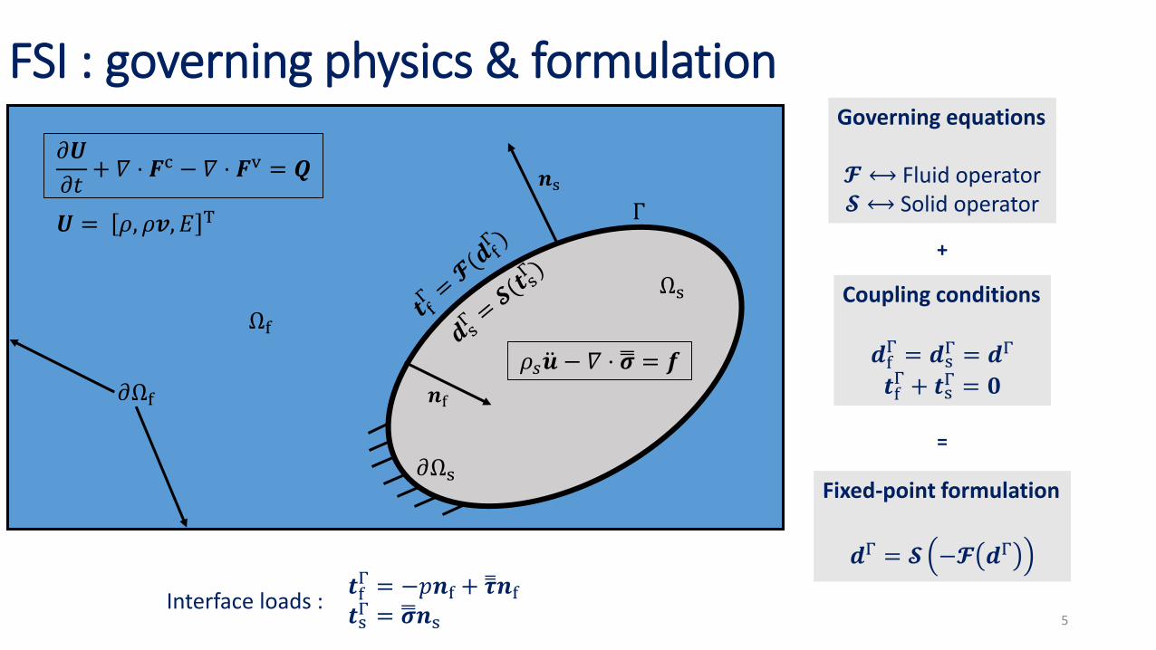
FSI : governing physics & formulation

Ωf

Ωs

Γ

Coupling conditions

𝒅fΓ = 𝒅s

Γ = 𝒅Γ

𝒕fΓ + 𝒕s

Γ = 𝟎

Governing equations

𝓕⟷ Fluid operator𝓢 ⟷ Solid operator

Fixed-point formulation

𝒅Γ = 𝓢 −𝓕 𝒅Γ

𝒏s

𝒏f

+

=

𝜕𝑼

𝜕𝑡+ 𝛻 ⋅ 𝑭c − 𝛻 ⋅ 𝑭v = 𝑸

𝜌𝑠 ሷ𝒖 − 𝛻 ⋅ ന𝝈 = 𝒇

𝒕fΓ = −𝑝𝒏f + ധ𝝉𝒏f𝒕sΓ = ന𝝈𝒏s

𝑼 = 𝜌, 𝜌𝒗, 𝐸 T

Interface loads :

𝜕Ωf

𝜕Ωs

5

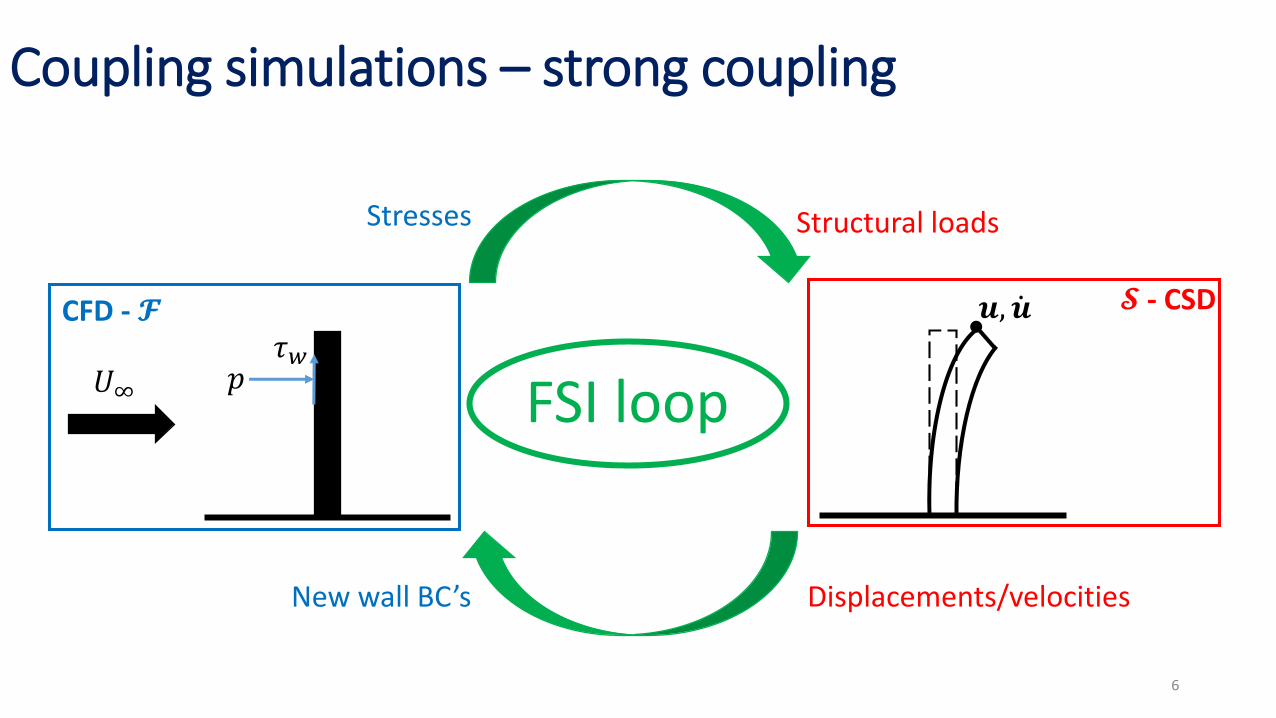
Coupling simulations – strong coupling

𝑈∞ 𝑝𝜏𝑤

𝒖, ሶ𝒖

FSI loop

CFD - 𝓕 𝓢 - CSD

Stresses Structural loads

Displacements/velocitiesNew wall BC’s

6

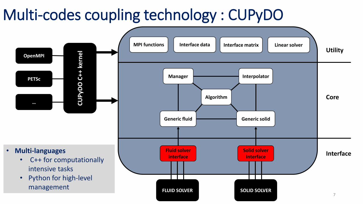
Multi-codes coupling technology : CUPyDO

FLUID SOLVER

Manager Interpolator

Algorithm

Generic fluid Generic solid

MPI functions

CU

PyD

OC

++

kern

el

Interface data Interface matrix Linear solver

Fluid solverinterface

Solid solverinterface

PETSc

OpenMPI

…

Utility

Core

Interface

SOLID SOLVER

• Multi-languages• C++ for computationally

intensive tasks• Python for high-level

management7

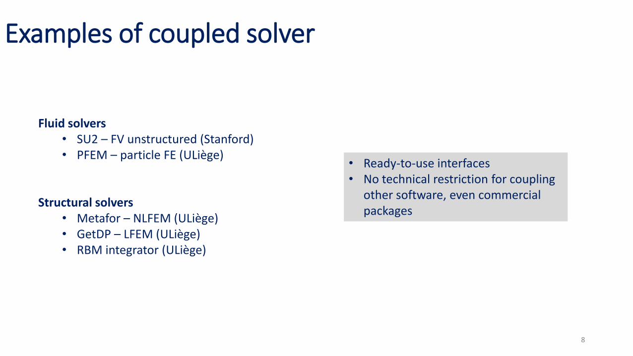
Examples of coupled solver

8

Fluid solvers• SU2 – FV unstructured (Stanford)• PFEM – particle FE (ULiège)

Structural solvers• Metafor – NLFEM (ULiège)• GetDP – LFEM (ULiège)• RBM integrator (ULiège)

• Ready-to-use interfaces• No technical restriction for coupling

other software, even commercial packages

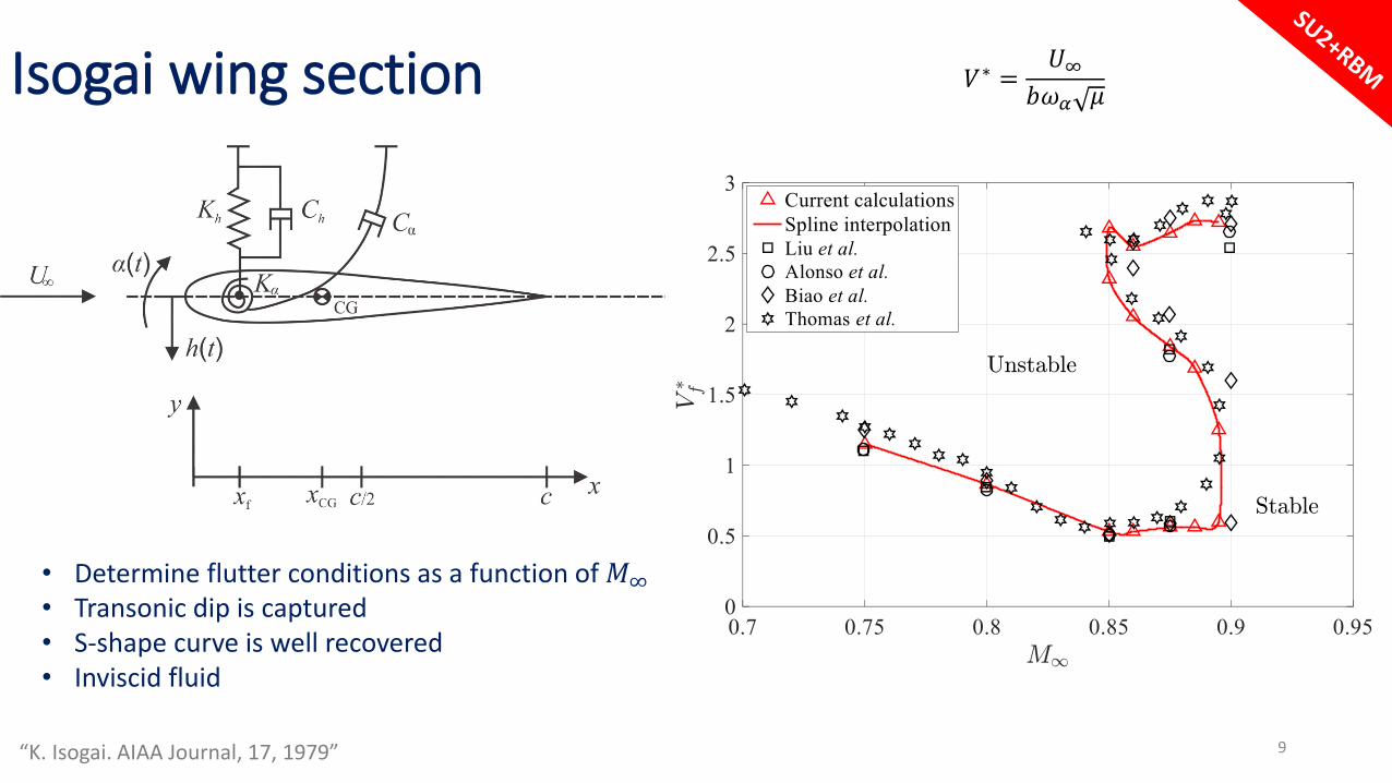
Isogai wing section

“K. Isogai. AIAA Journal, 17, 1979”

• Determine flutter conditions as a function of 𝑀∞

• Transonic dip is captured• S-shape curve is well recovered• Inviscid fluid

9

𝑉∗ =𝑈∞

𝑏𝜔𝛼 𝜇

Isogai wing section

• Moving shock interacting with the motion of the airfoil• Existence of a LCO due to nonlinear aerodynamics

10

Mach [-]: 0 0.2 0.4 0.6 0.8 1 1.2 1.4 1.6

𝑀∞ = 0.875𝑉∗ = 1

Stall flutter of a flat plate

“X. Amandolese et al., Journal of Fluids and Structures, 43, 2013.”

• Airfoil motion rapidly turns into stall flutter

• Induced by dynamic flow separation

• Nonlinearities lead to LCO

11

||U|| [m/s]: 0 2 4 6 8 10 12 14 16 18 20

𝑈∞ = 13 m/s

VIV of a flexible cantilever

“C. Habchi et al. , Computer & Fluids, 71, 2013.”12

• Solid motion is generated by vortex shedding

• Large displacement amplitude (nonlinear)

• Laminar flow at Re = 333

||U|| [m/s]: 0 0.1 0.2 0.3 0.4 0.5 0.6 0.7 0.8

VIV of a flexible cantilever

• From dense to light material• Low mass ratios = numerical coupling instabilities ➔ relaxation needed in coupling• Number of coupling iterations per time step increases

𝜌𝑠𝜌𝑓

≈ 100

13

𝜌𝑠𝜌𝑓

≈ 10𝜌𝑠𝜌𝑓

≈ 1

||U|| [m/s]: 0 0.1 0.2 0.3 0.4 0.5 0.6 0.7 0.8

ഥ𝑁𝐹𝑆𝐼 = 2.7𝑓 = 3.14 Hz

ഥ𝑁𝐹𝑆𝐼 = 6.9𝑓 = 7.26 Hz

ഥ𝑁𝐹𝑆𝐼 = 31.9𝑓 = 6.2 − 9.8 Hz

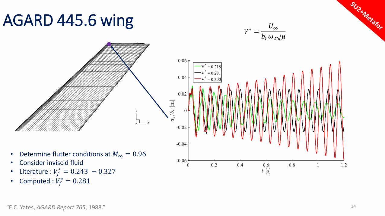
AGARD 445.6 wing

“E.C. Yates, AGARD Report 765, 1988.” 14

• Determine flutter conditions at 𝑀∞ = 0.96• Consider inviscid fluid• Literature : 𝑉𝑓

∗ = 0.243 − 0.327

• Computed : 𝑉𝑓∗ = 0.281

X

Y

Z

𝑉∗ =𝑈∞

𝑏𝑟𝜔2 𝜇

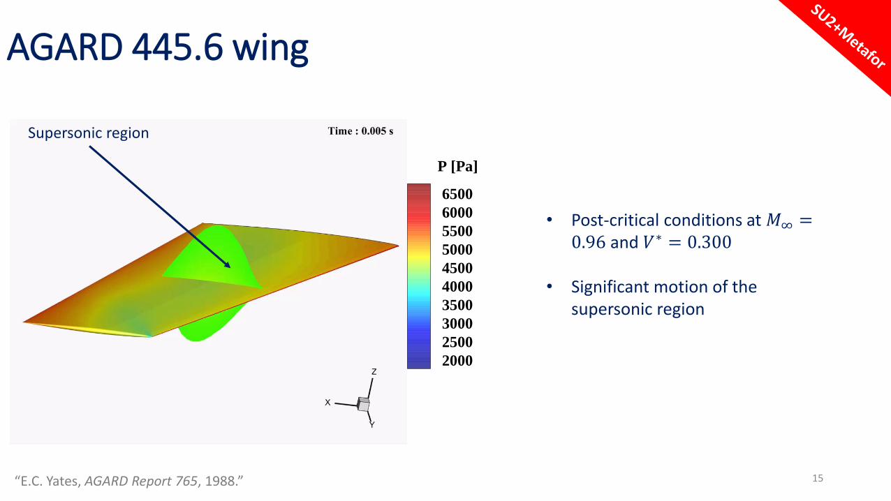
AGARD 445.6 wing

• Post-critical conditions at 𝑀∞ =0.96 and 𝑉∗ = 0.300

• Significant motion of the supersonic region

Supersonic region

15“E.C. Yates, AGARD Report 765, 1988.”

P [Pa]

6500

6000

5500

5000

4500

4000

3500

3000

2500

2000

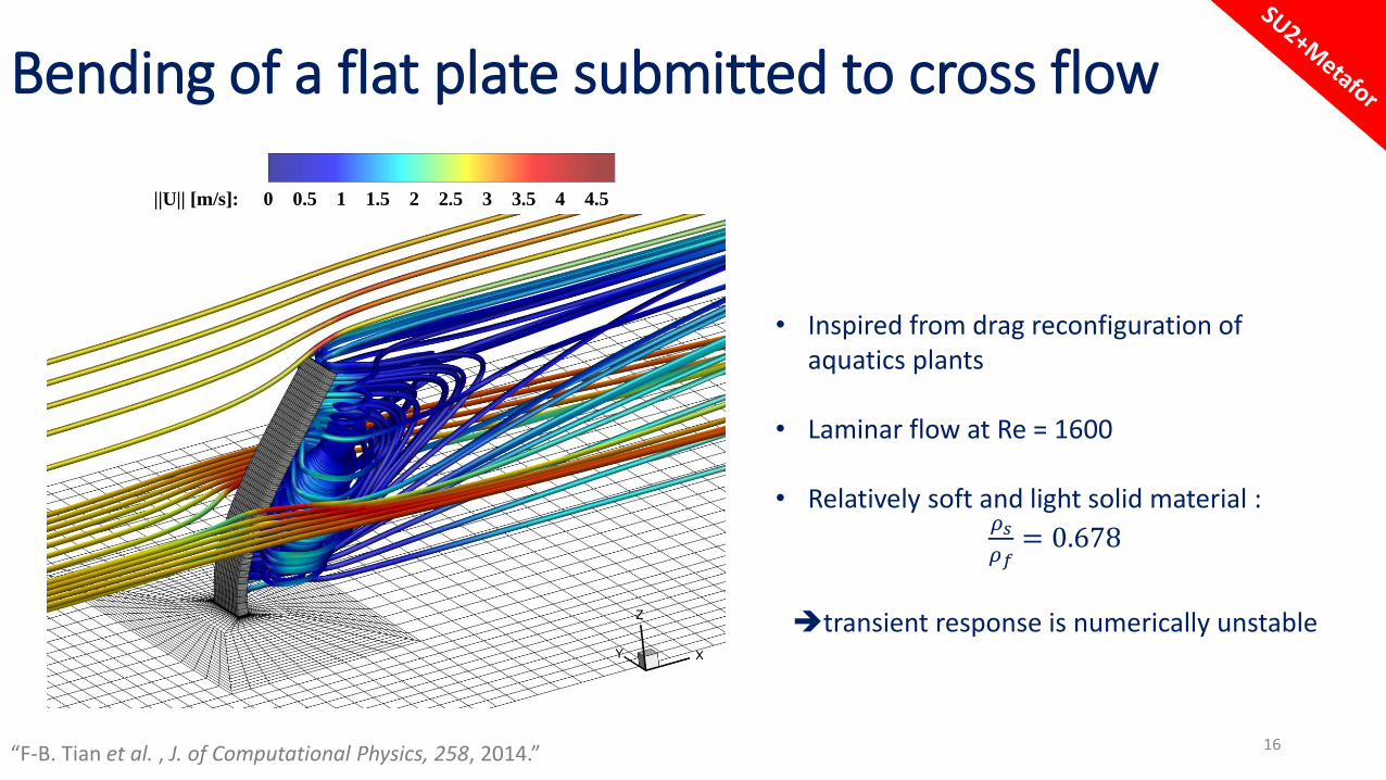
Bending of a flat plate submitted to cross flow

• Inspired from drag reconfiguration of aquatics plants

• Laminar flow at Re = 1600

• Relatively soft and light solid material :𝜌𝑠

𝜌𝑓= 0.678

➔transient response is numerically unstable

16

||U|| [m/s]: 0 0.5 1 1.5 2 2.5 3 3.5 4 4.5

“F-B. Tian et al. , J. of Computational Physics, 258, 2014.”

Cantilever flat wing

17

• Material : aluminium | Fluid : air• High aspect ratio plate with very small thickness• Very flexible structure

||V|| [m/s]: 0 0.05 0.1 0.15 0.2 0.25 0.3 0.35 0.4 0.45 0.5 ||V|| [m/s]: 0 0.1 0.2 0.3 0.4 0.5 0.6 0.7 0.8 0.9 1 1.1 1.2 1.3

𝑈∞ = 17.1 m/s𝑡∗ = 0.01 s𝑓 = 6.2 Hz

𝑈∞ = 17.1 m/s𝑡∗ = 0.1 s𝑓 = 9.8 Hz

• Two perturbation amplitudes• Two distinct limit cycles

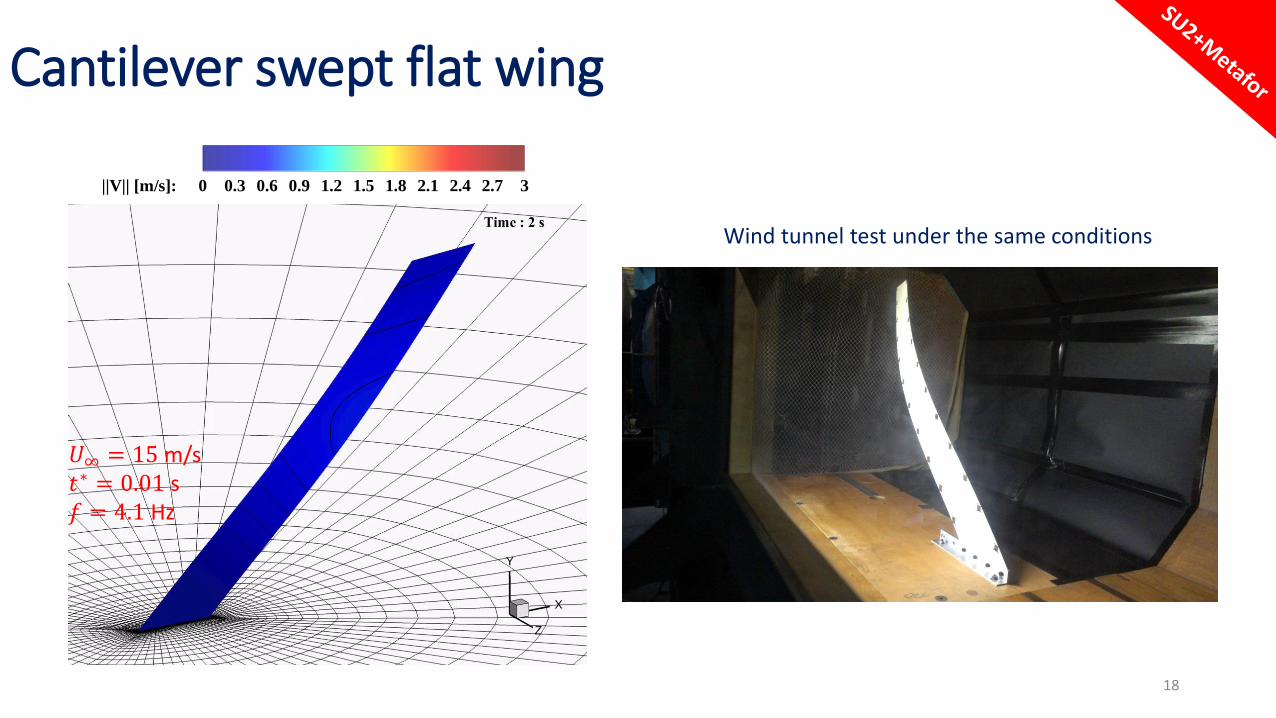
Cantilever swept flat wing

18

||V|| [m/s]: 0 0.3 0.6 0.9 1.2 1.5 1.8 2.1 2.4 2.7 3

Wind tunnel test under the same conditions

𝑈∞ = 15 m/s𝑡∗ = 0.01 s𝑓 = 4.1 Hz

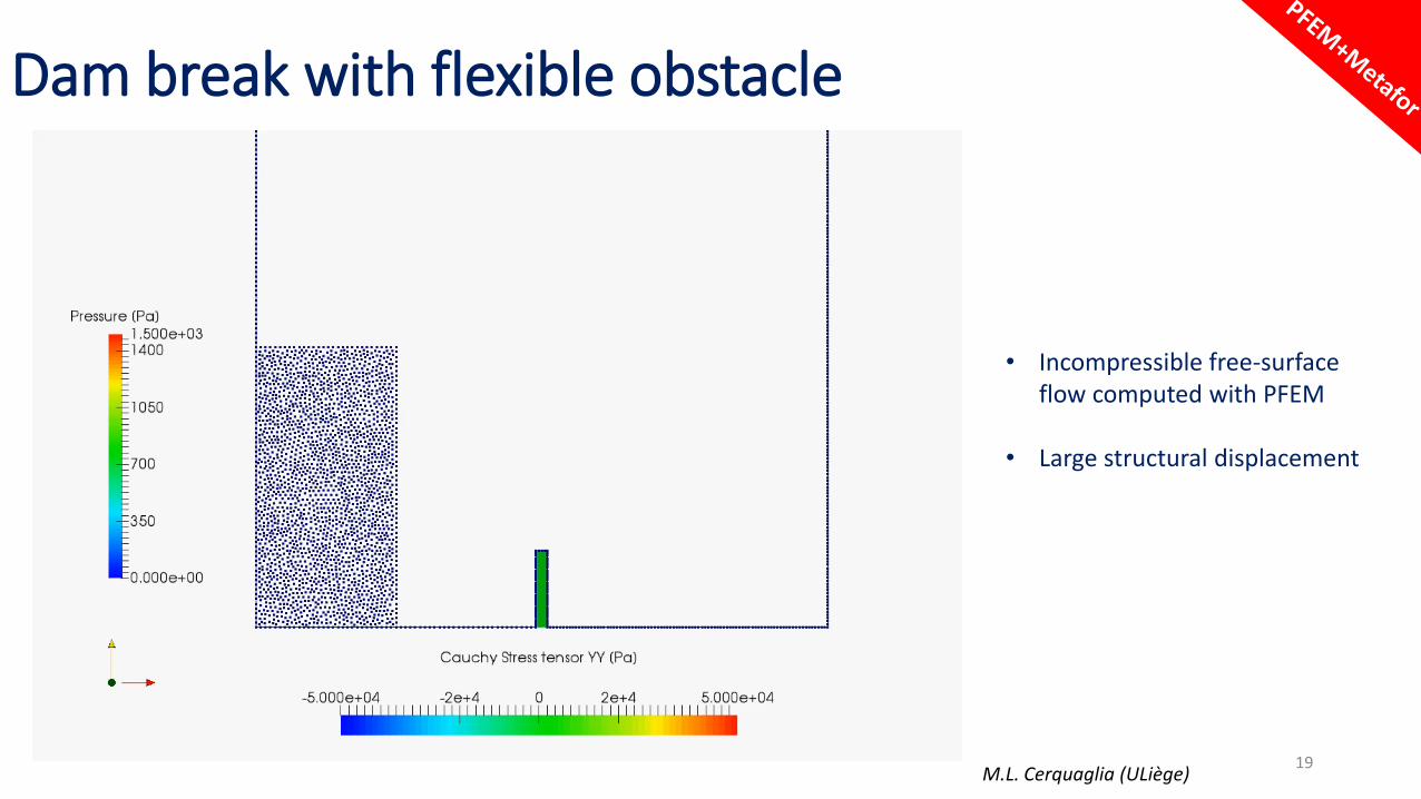
Dam break with flexible obstacle

M.L. Cerquaglia (ULiège)19

• Incompressible free-surface flow computed with PFEM

• Large structural displacement

Conclusions

• Developed for research and design

• Interfacing tool for strong coupling of independent solvers

• High fidedility models for nonlinear FSI

• Flexible partitioned tool for large range of physics

• Validated on typical benchmarks

20

Acknowledgements

21