democratic accountability in open economies
TRANSCRIPT
Democratic Accountability in Open Economies∗
Thomas SattlerSchool of Politics andInternational Relations
University College [email protected]
Patrick T. BrandtSchool of Economic, Political
and Policy SciencesThe University of Texas, Dallas
John R. FreemanDepartment of Political Science
University of [email protected]
March 23, 2010
Abstract
We analyze democratic accountability in open economies based on different hypothesesabout political evaluations and government responsiveness. Specifically, we assess whethercitizens primarily rely on government policies or if they focus on economic outcomes result-ing from these policies to evaluate governments. Our empirical analysis relies on Bayesianstructural vector autoregression models for the British economy, aggregate monthly measuresof public opinion, and economic evaluations from 1984–2006. We find that voters continuouslymonitor and strongly respond contemporaneously to changes in monetary and fiscal policies,but less to changes in macroeconomic outcomes. Voters also respond to policies differentlywhen institutions change. When the Bank of England became politically independent, citizensshifted their attention toward fiscal policy, and the role of monetary policy in their evaluationsdecreased significantly. Finally, politicians respond to voting behavior by adjusting their poli-cies in a sensible way. When vote intentions and approval decrease, the government reacts tothe public by adjusting fiscal policy and, before the Bank of England became independent, alsomonetary policy.
∗Earlier versions of this paper were presented at the Conference on the Political Economy of International Finance(PEIF), Federal Reserve Bank Atlanta, February 9, 2007, and the Seminar of the Center for the Study of DemocraticPolitics, Princeton University, October 25, 2007. Brandt’s and Freeman’s research was sponsored by the NationalScience Foundation under grants numbers SES-0351179, SES-0351205 and SES-0540816. Sattler’s research wassupported by the Swiss National Science Foundation under grant number 101412-101962/1. Harold Clarke kindlyprovided data on subjective personal expectations. We thank William Bernhard, Mark Hallerberg, Jude Hays, TimHellwig, Patrick Kuhn, David Leblang, Angela O’Mahony, Thomas Plumper, Dennis Quinn, Ken Scheve, the anony-mous referees and the editors for comments. The authors are solely responsible for the contents.
1
It is a fundamental idea of modern democratic politics that citizens evaluate their government
and hold it accountable for its performance. Citizens can do this in different ways. In a recent,
major contribution, Duch and Stevenson (2008) applied a competence model to this problem. They
stressed the importance of outcomes, which are realizations of policies subject to random shocks
and thus containing noisy signals about policymakers’ competence. An alternative hypothesis is
that citizens primarily evaluate policies that governments choose to draw conclusions about the
quality of government decisions.
We use an empirical framework that allows us to examine these hypotheses. It is based on a
Bayesian structural vector autoregression model for the British economy, aggregate public opinion,
and economic evaluations. We use this framework to examine the mechanism connecting observ-
able and unobservable government policies, economic performance and citizens’ evaluations of
economic developments. Because its economy is only moderately open to trade and capital flows,
it has a relatively small state, its regulation density is low, and wage bargaining is decentralized,
democratic accountability, based on the competence model(s), ought to exist in Britain (Duch and
Stevenson, 2008).
We find that in Britain, voters respond to policies more than to the outcomes that result from
these policies. Specifically, vote intentions and prime minister approval respond strongly to changes
in monetary and fiscal policies, but considerably less to measures of economic outcomes. Voters
also respond to policies differently when institutions change. When the Bank of England be-
came politically independent, citizens shifted their attention toward fiscal policy, and the role of
monetary policy in evaluations decreased significantly. Politicians respond to voting behavior by
adjusting their policies in a sensible way. When vote intentions and approval decrease, the gov-
ernment reacts to the public by adjusting fiscal policy and, before the Bank of England became
independent, also monetary policy. These results suggest that theoretical models should assign
greater relevance to the role of policies for government evaluations.
2
Theory
Competence model(s) of democratic accountability emphasize macroeconomic outcomes that al-
low citizens to draw conclusions about the quality of decisions made by their representatives
(Persson and Tabellini, 1990; Alesina and Rosenthal, 1995; Duch and Stevenson, 2008) If citi-
zens perceive that economic performance has been good, then they infer that their incumbent is
competent, and are more likely to support that incumbent. The nature of the information that cit-
izens infer from economic performance—especially, the strength of the incumbent’s competency
signal—differs across countries and time, in part, because of the workings of political and eco-
nomic institutions.
In essence, competence model(s) rely on retrospective evaluation of economic outcomes weighted
by a signal extraction about competence within a given institutional setting. Citizens know the nat-
ural rate of growth in an economy and the competency of the incumbent in the past. To a certain
degree, they also have information about the current competence of the incumbent, although not
the complete information that they possess about past competence. This knowledge allows them
to form rational expectations about their expected utility of supporting the incumbent over a chal-
lenger. Specifically, if current, observed economic performance is good relative to the natural rate
of growth and past competence level, and the current competency signal is strong, then citizens
rationally choose to vote for the incumbent; voting for the incumbent is more likely to benefit them
in the future in comparison to the benefit that might accrue from voting for the challenger.1
1Duch and Stevenson (2008) derive the expected utility of voting for an incumbent as opposed for a challenger
whose competence is unknown using
E� α�
l=1
µi|t+1|vi
�− E
� α�
l=1
µk|t+1|vk
�= b
� ασ2µ
ασ2µ + βσ2
ψ
��yit − y −
α�
l=1
µi|t−1
�
where yit is the observed current growth under incumbent i, y is the natural rate of growth and µt−1 is past competence
of the incumbent, all of which are known to the voters. The variables vi and vk are votes for the incumbent or
the challenger, respectively and the parameters α and β capture the number of decisions made by elected and non-
elected decision-makers, respectively. The variances σ2µ and σ2
ψ capture the volatility in the political (competency) and
3
In these models, the larger idea of democratic accountability is embedded in two interconnected
causal links. The first is a citizen-evaluation link that specifies how citizens judge government per-
formance based on observed and unobserved behavior (characteristics) of elected officials. The
second is the competence-outcome link that reflects incumbents’ skills or expertise. The latter is
grounded in a Lucas supply function, a single equation that stipulates that current growth can de-
part from the natural rate when the inflation rate deviates from the expected inflation rate, when
incumbents produce surprise shocks of various (unspecified) kinds, or when an unexpected nonpo-
litical shock is experienced by the economy. Incumbents and challengers know that the inflation
rate negatively enters the voters’ value function, and, regardless of their partisan identity, they gen-
erally choose zero inflation. Because voters anticipate this, inflation does not play a major role
for their vote. The accountability mechanism therefore works through the unexpected shocks that
voters observe.
The shock has two components, a nonpolitical (exogenous) shock that is beyond the control of
public officials and (past and current) competence shocks that can be assigned to incumbents.2 By
producing positive shocks, competent incumbents can increase economic growth above the natural
rate. Voters know only the variance of the shocks that incumbents produce relative to the variance
of nonpolitical shocks. The ratio of the former variance to the sum of the two variances is the
competence signal that they use to weight their retrospective evaluations of the economy. If this
ratio is relatively large and retrospective evaluations are positive (negative), then they hold their
incumbents accountable for past performance, voting to retain (replace) them. If the ratio is small,
i.e., the size of the variance of political shocks is small relative to the size of the variance of the
nonpolitical shocks, then voters do not hold incumbents responsible for past performance; little or
no economic voting is observed in this case.
Duch and Stevenson (2008) show that voters’ abilities to extract competence signals from ob-
nonpolitical shocks that the economy experiences.2In Duch and Stevenson’s (2008) investigation, the economic shock in the Lucas supply function, yit = y + πit −
πeit + ηit, can be divided into two parts, ηit = �it + ξt, where �it is the competency shock and ξt is the nonpolitical
shock, both at time t. Competency depends on policymakers’ past and current competence, �it = µit + µit−1.
4
served economic performance varies across contexts. The more non-elected officials are involved
in economic decision-making, the less elected incumbents are held accountable for economic out-
comes: in terms of the model, the competency signal weight is smaller in this case, hence the
expected value of voting for the incumbent over the challenger is relatively smaller. The relative
importance of elected decision-makers decreases and hence the competency signal is necessar-
ily weaker, the more the domestic economy is integrated into the world economy, the greater the
size of government, the greater the regulatory density of government activity, and (or) the more
wage bargaining is centralized. These factors restrict the ability of elected officials to influence
economic performance and increase the influence of bureaucrats, non-governmental officials or
private economic actors on the economy. Citizens take this into account and assign less weight to
past economic performance in the respective contexts.
An implication of many competence model(s) is that they assign importance to economic out-
comes. The competence of policymakers can be most reliably inferred from past macroeconomic
developments, specifically economic growth. Observable policies, specifically monetary and fiscal
policies, play a negligible role for citizens’ evaluations in these models. Monetary policy decisions
do not bear on competence because incumbents and challengers always choose zero inflation. Fis-
cal policy, the most important policy tool of governments in a country with an independent central
bank, does not appear in these models at all.
Previous research, however, suggests that citizens take into account a broader range of infor-
mation that also includes policy choices when they evaluate governments. Many policies are easily
observable and can be instantaneously evaluated by citizens. For instance, interest rates, a major
component of monetary policy, are constantly reported in the news. Similarly, many, if not most,
fiscal decisions are publicly known because they are debated in parliaments and in the media. Ac-
cordingly, there is evidence that citizens respond to changes in easily observable monetary policy
instruments, such as interest rates, at least in institutional settings where elected policymakers have
control over monetary policy (Sanders, 1991). Publicly known fiscal policy decisions, such as tax
rates, play an important role in citizen evaluations of their governments, especially when elected
5
officials are not in charge of monetary policy (Sanders, 2005). The implication is that evaluations
and hence accountability may depend on both policy choices and macroeconomic outcomes or
even policy alone.
Unlike an evaluation mechanism that focuses on outcomes only, the possibility that citizens
evaluate policies instead of outcomes requires a discussion of the institutional framework within
which economic policy is made. In the past when central banks were not independent, monetary
policy decisions can be attributed to the elected government and thus should matter for evaluations
Bernhard, Broz and Clark (2002). When central banks became independent, we should observe a
shift towards fiscal policy, which then becomes the main policy tool of the elected government. In
this way, institutional change can affect citizens’ evaluations and accountability, but through policy
evaluation and not outcome evaluation.
Empirical Assessment of Democratic Accountability
A General Open Political Economy Framework
To assess how citizens evaluate governments and how government respond to these evaluations,
we construct an empirical model that encompasses the three essential parts of an open political
economy. These three parts include the public, an economy, which is divided into a domestic
and the international economy, and a government. First, the public reflects how citizens continu-
ously assess the economic developments and policies. It is represented by different measures of
public opinion, specifically vote intentions (vt), approval of the chief executive’s work (at), and na-
tional economic and personal financial expectations (net and pet). Second, the economy is divided
into domestic and international sectors to model the economic interdependence of a contemporary
economy, the former represented with d superscripts, the latter, with i superscripts. The domestic
and international economic variables are domestic and international prices and output (pdt , pi
t, ydt
and yit), foreign monetary policy (ri
t), and an exchange rate (et). Third, the government consists of
two distinct actors, a monetary and a fiscal policy authority conducting monetary and fiscal policy
6
(rdt and gt). Depending on central bank independence, the polity and the economy are expected to
receive different weights in the monetary and fiscal reaction functions. We also include an election
counter.
The polity in our framework includes the most important components of existing models of eco-
nomic evaluations of governments and government popularity in general (Erikson, MacKuen and
Stimson, 2002; Clarke et al., 2004; Sanders, 1991, 2005; Duch and Stevenson, 2008). Research on
representation in economic policy that links policy outcomes to public opinion addresses govern-
ment behavior (Stimson, MacKuen and Erikson, 1995; Wlezien, 2004; Soroka and Wlezien, 2005).
We extend this literature by connecting policy, economic outcomes, and government evaluations.
This complete evaluation mechanism has not been explicitly modeled in previous research. This
nexus between policy and outcomes coincides with research from New Open Macroeconomics
that analyzes policy effects and interdependencies in open economies (Obstfeld and Rogoff, 1995;
Cushman and Zha, 1997; Kim, 2001). Our framework thus accounts for international factors that
have been omitted from political models of economic policymaking despite a general consensus
that globalization has important effects on domestic policymaking. In essence, our framework al-
lows us to sort out more completely the linkages between citizens’ evaluations, observed economic
policies and macroeconomic outcomes.
Empirical Approach
Modeling the multiple time series described in the last section requires a system of equations. In
the econometrics and time series literature there are three generally accepted options for analyzing
such a dynamic system: a) simultaneous equation models, b) (vector) error correction models and
c) vector autoregressions. Freeman, Williams and min Lin (1989) and Brandt and Williams (2007)
outline the relative tradeoffs in the selection of these models. A simultaneous equation specifi-
cation requires the analyst to make assumptions about the (weak) exogeneity of the variables in
the model. The theoretical accounts of democratic evalutions outlined earlier do not provide these
kinds of identification restrictions. Further, simultaneous equation models are special cases of un-
7
restricted vector autoregression models (Sims, 1972, 1980). A vector error correction specification
requires that the analyst investigate the error correction relationships among the unit root variables
in the model. This is not the goal of this analysis and is a special case of vector autoregression
models (Brandt and Williams, 2007; Sims, Stock and Watson, 1990). Finally, one could adopt
a reduced form perspective that does not model the relevant contemporaneous relationships. But
this is contrary to the over decade-long literature in applied macro-economics that uses (Bayesian)
structural vector autoregression models to account for these relationships (e.g., Cushman and Zha,
1997; Leeper, Sims and Zha, 1996; Sims and Zha, 1998; Sims, Waggoner and Zha, 2008).3
To assess the causal relationships among the variables in the open political economy frame-
work, we construct a Bayesian, structural vector autoregression (B-SVAR) model (Brandt and
Freeman, 2006, 2009). This model treats the system of variables as fully endogenous. The model
takes the following form:
A0Yt +p�
j=1
AjYt−j = DZt + �t, �t ∼ N(0, I), t = 1, . . . , T. (1)
The A0 is a 12× 12 matrix that defines the contemporaneous relationships among the endogenous
variables and Yt is a 12 × 1 vector of endogenous variables at time t. The vector Yt contains the
polity, policy, and open economy variables discussed previously. The Aj are the 12× 12 matrices
of the structural coefficients for the lagged endogenous variables Yt−j at lag t − j, Zt is a 2 × 1
vector of the electoral counter and a constant, D is a 12× 2 matrix of the structual coefficients for
the exogenous variables, and �t is a 12× 1 vector of normal i.i.d. structural shocks. The details of
the estimation of this model are outlined in the appendix.
To draw inferences about the causal relationships among the endogenous variables in Yt, we3Many specious criticisms of vector autoregression modeling exist in political science. Nevertheless, vector au-
toregression models are workhorses in the empirical macroeconomics, time series analysis, and statistics. The vector
autogression model is not inherently atheoretical: it captures the baseline correlations among the time series in the
model. The interpretation and decomposition of these correlations depends on the theoretical insights brought to the
analysis by the researcher (Williams, 1990; Brandt and Williams, 2007).
8
impose restrictions (a structure) on the contemporaneous relationships among the variables, A0
(Brandt and Freeman, 2009). This structure corresponds to the theoretical and empirical results
about which endogenous variables influence each other within the same time period, and which do
not. We use monthly data to estimate the model, which means that the A0 matrix specifies how
the endogenous variables influence each other within the same month. Imposing restrictions on the
contemporaneous relationships does not exclude the possibility that variables can influence each
other with a lag or delay. We do not impose restrictions on the lagged relationships among the
endogenous variables, which are captured by the matrices Aj , j = 1, . . . , p.
To assess citizens’ evaluation mechanisms, we proceed in two steps. First, we define different
structural specifications for the contemporaneous relationships among public opinion, economic
and policy variables. These structural specifications reflect different hypotheses about public eval-
uations and policy derived from the theoretical discussion and the broader political economy litera-
ture. For instance, the competence models(s) imply that public opinion does not react to changes in
observable economic policy and therefore observable policy does not necessarily respond to public
opinion. We first test this hypothesis against the alternative that citizens closely monitor govern-
ment behavior as represented by observable policy choices. As suggested by Duch and Stevenson
(2008), we also construct different specifications that reflect the idea that the impacts of monetary
and fiscal policies vary with and without central bank independence.
Second, we examine the causal linkages among the variables for the best performing empirical
specification, which allows us to discriminate between the different causal evaluation mechanisms.
If we observe only a weak link between observable economic policy and evaluations, then this
would be evidence in favor of the hypothesis that citizens mostly focus on economic outcomes
instead of policies. If we are able to establish a strong connection between evaluations and observ-
able policy and (or) between these evaluations and specific policy innovations (shocks), then this
would be evidence in favor of the alternative hypothesis.
For the first part of the analysis, we allow for varying contemporaneous relationships across
the polity and the economy, while the contemporaneous relationships within the polity and the
9

economy are fixed. Thus, we focus on the intersections between the polity and the economy and
partition the A0 matrix and Yt vector into four parts. These partitions describe the endogenous
relationships among the economy and polity variables in our model. We do this by partitioning the
A0 matrix and Yt as follows:
A0Yt =
�AE
0 APE0
AEP0 AP
0
� �Y E
t
Y Pt
�=
�AE
0 Y Et + APEY P
t
AEP0 Y E
t + AP Y Pt
�, (2)
where the vectors Y Et and Y P
t are the variables for the economy and polity in Yt,
Y Et =
�et rd
t rit gt pd
t ydt pi
t yit
�� (3)
Y Pt =
�net pet at vt
��. (4)
The matrices AE0 and AP
0 capture the contemporaneous relationships within the economy and the
polity, respectively. The matrix AE0 describes how the economic and economic policy variables
react to each other within the same month. The matrix AP0 indicates how the public opinion vari-
ables respond to each other within the same month. The contemporaneous relationships among the
variables within the polity and the economy are fixed for all models. The matrices AE0 and AP
0 thus
are the same for the different specifications. The justifications for their structures are discussed in
detail in the Appendix.
The matrices APE0 and AEP
0 represent the contemporaneous relationships across the polity and
the economy. The APE0 matrix describes contemporaneously how politics affects the economy,
or how economic and policy variables react to changes in opinion variables. The AEP0 matrix
reflects how the economy contemporaneously affects politics, i.e., how political opinion variables
react to changes in the economy and economic policy. So consider these as the first superscript
contemporaneously causes the second—in a very specific way. These two matrices differ for the
different specifications and we discuss them in detail below.
The first step of the democratic accountability mechanism examines how citizens and hence
public opinion reacts to government policy and the economy. The contemporaneous reactions of
10
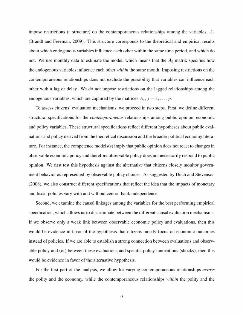
the public opinion equations to economic policy are captured in the AEP0 submatrix of Equation 2.
We specify the relationships in AEP0 as
AEP0 Y E
t =
0 αMEP,1 0 αF
EP,5 0 0 0 00 αM
EP,2 0 αFEP,6 0 0 0 0
0 αMEP,3 0 αF
EP,7 0 0 0 00 αM
EP,4 0 αFEP,8 0 0 0 0
et
rdt
rit
gt
pdt
ydt
pit
yit
=
αMEP,1r
dt + αF
EP,5gt
αMEP,2r
dt + αF
EP,6gt
αMEP,3r
dt + αF
EP,7gt
αMEP,4r
dt + αF
EP,8gt
. (5)
Equation 5 represents the contribution of the two policy variables, interest rates and spending
(rdt and gt), to the equations for the four political variables in Equation 4: national economic
expectations (net), personal financial expectations (pet), chief executive approval (at) and vote
intentions (vt), respectively. None of the coefficients on policy in the public opinion equations
is restricted to be zero. Both policy variables (potentially) contemporaneously affect the public
opinion.
The second and fourth columns of matrix AEP0 that produce Equation 5 determine how the
four opinion variables react to monetary and fiscal policy. The coefficients αMEP,1 through αM
EP,4
reflect how monetary policy changes influence national economic expectations, personal financial
expectations, chief executive approval and vote intentions, respectively. The coefficients αFEP,5
through αFEP,8 show how fiscal policy affects the same public opinion variables. As an example,
αMEP,4 is the contemporaneous coefficient for how domestic monetary policy, rd
t affects the vote
intention function. It tells us how vote intentions change within the same month when domestic
monetary policy changes.
The competence model(s) implies that citizens do not monitor government policy and do not
reward the government with more support if the government adjusts observable policies. If citi-
11
zens nonetheless observe and evaluate policy, then they would mostly care about monetary policy
because inflation negatively enters their value functions. Monetary policy choices that increase
inflationary expectations would lead to lower political support for the government, (but such a be-
havior is not explicitly predicted by the competence model(s)). In our empirical model, this means
that the coefficients in AEP0 should be restricted because the opinion variables should not respond
to policy variables. With respect to monetary policy, this means that the following restrictions
hold:
αMEP,1 = αM
EP,2 = αMEP,3 = αM
EP,4 = 0. (6)
While the implications of competence model(s) for monetary policy are clear, the model is not
explicit about the exact role of observable fiscal policy. Besides monetary policy which determines
inflation, government’s fiscal decisions and their effects are also unobservable. We infer from
this setup that observable fiscal policy choices are not important for accountability and citizens’
evaluations. Public opinion thus should not react to fiscal policy choices. This means that opinion
variables do not respond to the fiscal policy variable, or that in Equation 5,
αFEP,5 = αF
EP,6 = αFEP,7 = αF
EP,8 = 0, (7)
for the opinion variables’ contemporaneous responses to the fiscal variables.
As noted above, the competence model(s) has no reaction functions per se. But much of
the political economy literature suggests that the government infers from public opinion what
citizens expect in terms of economic policy and adjusts policy accordingly. Monetary and fiscal
policy variables thus should respond immediately to changes in national economic and personal
financial expectations, prime ministerial approval and vote intentions. In our model, this policy
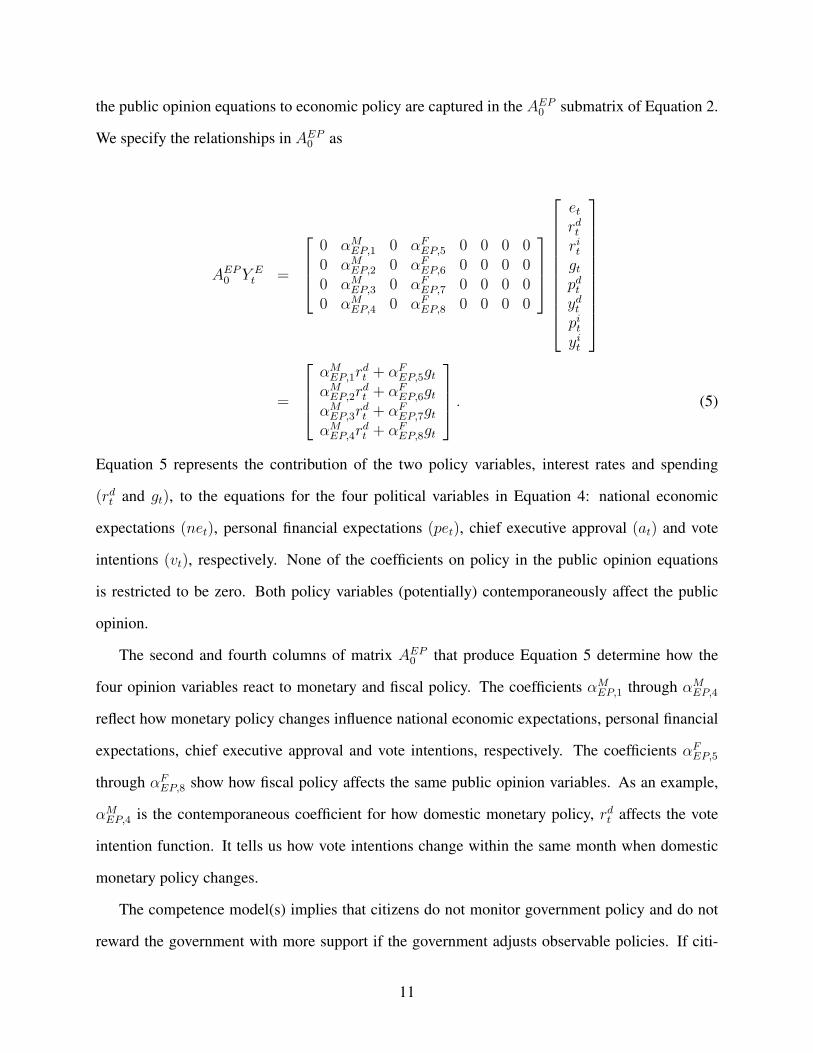
responsiveness is captured in the matrix APE0 . The submatrix for the APE
0 Y Pt relationships for our
model in Equation 2 are given by
12

APE0 Y P
t =
αXPE,1 αX
PE,2 αXPE,3 αX
PE,4
αMPE,5 αM
PE,6 αMPE,7 αM
PE,8
0 0 0 0αF
PE,9 αFPE,10 αF
PE,11 αFPE,12
0 0 0 00 0 0 00 0 0 00 0 0 0
net
pet
at
vt
=
αXPE,1net + αX
PE,2pet + αXPE,3at + αX
PE,4vt
αMPE,5net + αM
PE,6pet + αMPE,7at + αM
PE,8vt
0αF
PE,9net + αFPE,10pet + αF
PE,11at + αFPE,12vt
0000
. (8)
Equation 8 captures the contribution of the four polity variables to the equations eight economic
variables in Equation 3. The first four economic are the exchange rate (et), domestic monetary
policy (rdt ), foreign monetary policy (ri
t) and domestic fiscal policy (gt). Note that none of the
domestic polity variables contemporaneously enter the equations for foreign monetary policy. All
four of the polity variables (potentially) contemporaneously affect the exchange rate, domestic
monetary policy, and fiscal policy equations.4
In the matrix in Equation 8, the second and fourth rows reflect how the public opinion vari-
ables affect monetary and fiscal polices, respectively. The coefficients αMPE,5 through αM
PE,8 are the
coefficients on national economic expectations, personal financial expectations, chief executive ap-
proval and vote intentions, respectively, in the monetary reaction function. The coefficients αFPE,9
through αFPE,12 are the coefficients on the same variables in the fiscal policy reaction function equa-
tion. In other words, the coefficients capture how monetary and fiscal policies contemporaneously
react to public opinion. Finally, the first row of matrix APE0 indicates how the exchange rate re-
sponds to the public opinion variables via the αXPE coefficients. Following Bernhard and Leblang
(2006) who find that political evaluations and exchange rate movements are causally related, we4The economy influences policy through matrix AE
0 which is discussed in the Appendix.
13
leave the parameters in this row unrestricted.
Finally, in the competence model(s), the government’s competence and therefore economic de-
cisions are exogenous. In this setup, we would expect that observable macroeconomic policy does
not respond to changes in public opinion and citizens’ evaluations of government performance.
Moreoever, in institutional settings where the elected government does not control monetary pol-
icy, domestic interest rates should not react to public opinion because the conservative central bank
exclusively focuses on price stability. In our model, this means that the coefficients in Equation 8
are restricted as follows:
αMPE,5 = αM
PE,6 = αMPE,7 = αM
PE,8 = 0. (9)
When the central bank is independent, it is plausible that fiscal responsiveness increases. The
government then resorts to its only remaining economic policy instrument—fiscal policy—to re-
spond to citizens’ evaluations. In other words, the coefficients αFPE,9 through αF
PE,12 are expected
to be non-zero when the bank is independent and zero when it is directly responsible to elected
officials. The larger implications of the model therefore suggest that coefficients on the opinion
variables in the fiscal reaction function in Equation 8 are zero as well, or
αFPE,9 = αF
PE,10 = αFPE,11 = αF
PE,12 = 0. (10)
Estimation and Testing
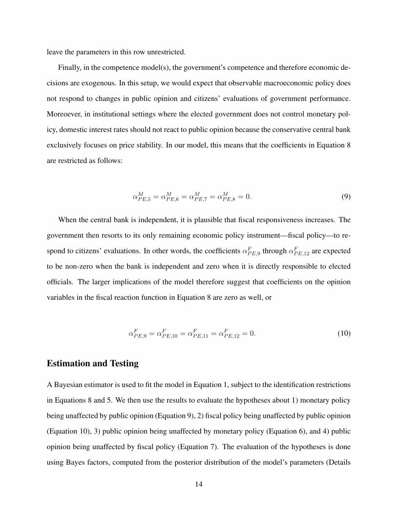
A Bayesian estimator is used to fit the model in Equation 1, subject to the identification restrictions
in Equations 8 and 5. We then use the results to evaluate the hypotheses about 1) monetary policy
being unaffected by public opinion (Equation 9), 2) fiscal policy being unaffected by public opinion
(Equation 10), 3) public opinion being unaffected by monetary policy (Equation 6), and 4) public
opinion being unaffected by fiscal policy (Equation 7). The evaluation of the hypotheses is done
using Bayes factors, computed from the posterior distribution of the model’s parameters (Details
14
are in the Appendix).
We estimated four specifications of the Bayesian structural vector autoregression (B-SVAR)
models. The first of these is the full Policy Linkage specification that allows for contemporaneous
feedback from monetary and fiscal policy to the public opinion measures and vice versa. This
model uses the specification based on Equations 8 and 5. The second, Monetary Linkage specifi-
cation allows only for contemporaneous effects of public opinion in monetary policy, but not fiscal
policy. This imposes the restrictions in Equations 7 and 10. The third, Fiscal Linkage specification
allows only for contemporaneous effects of public opinion in fiscal policy, but not monetary policy.
This imposes the restriction in Equation 6 and 9. Finally, we estimate a specification that allows
for No Linkage by imposing all four sets of restrictions on the A0 matrix. Models emphasizing the
role of outcomes instead of policies are most consistent with the last of these specifications.
The Bayesian estimation methods for B-SVAR model have been well described elsewhere, and
the interested reader should consult Waggoner and Zha (2003a,b) and Brandt and Freeman (2006,
2009). The only issues specific to the implementation of the Bayesian estimation here are 1) the
specification of the prior, and 2) the characterization of the posterior sample. The prior employed
for our models is a Sims-Zha prior for a structural VAR (Sims and Zha, 1998; Brandt and Freeman,
2006, 2009). This prior is centered on a random walk model (though the posterior need not be)
and assumes that higher order lag terms have smaller variances than lower ordered lag terms.5
Our final results are based on a posterior sample drawn via a Gibbs sampling method for B-
SVAR models (Waggoner and Zha, 2003a). The burn-in for the sampler was 10,000 draws, which
were discarded before drawing a final posterior sample of 25,000 draws, which passes standard
convergence diagnostics. All of the results reported below are based on this posterior sample.
Finally, to compare our four models we computed the log marginal data density for each of the
models. This is the log posterior density measure for a specification (Policy Linkage, Monetary5These prior beliefs are specified using a series of seven hyperparameter values. Specifically, we set the hyperpa-
rameter values at λ0 = 0.6, λ1 = 0.1, λ3 = 1, λ4 = 0.1, λ5 = 0.05, µ5 = µ6 = 5. These (and similar) values have
been widely used in the macroeconomics and political economy literature (e.g., Sattler, Freeman and Brandt, 2008;
Sims and Zha, 1998; Cushman and Zha, 1997). The resulting posterior inferences are robust to alternative values.
15
Linkage, etc.) in a given sample period. It is used to assess whether the specification generated
the sample. Log marginal data density values can be compared to generate Bayes factors which
measure the relative evidence or weight that should be given to a model in comparison to another,
exactly like a likelihood ratio statistic in frequentist analyses (Kass and Raftery, 1995).
We use impulse response functions (IRFs) to assess the impact of policy innovations (shocks)
on citizen evaluations and macroeconomic outcomes. The IRFs are an especially useful tool to
assess the predictions of the theoretical models. More detail about the estimation of the Bayesian
structural vector autoregression model is supplied in the Appendix.
Application to a Critical Case: Great Britain
Background
According to theories of macropolitical economy, democratic accountability should be most evi-
dent in countries whose economies are only moderately open to international trade and investment,
whose public sectors are relatively small, whose regulatory density is limited and whose wage bar-
gaining institutions are relatively decentralized (Duch and Stevenson, 2008, Ch. 5 and 7). The UK
is a country that satisfies most of these conditions. Its clarity of responsibility is very high be-
cause the UK is governed by a single-party government that can design economic policy without
interventions by other pivotal actors (Powell and Whitten, 1993). The shift to central bank inde-
pendence in 1997 also allows us to test whether under different institutional settings the changing
role of monetary and fiscal policy in the democratic evaluation mechanism. It is for this reason
that we split the sample and conduct analyses for the periods of Tory and Labour control of the
government. We recognize that this does not allow us to separate out the effects of partisan change
from central bank independence, but it does allow us to evaluate the presence of monetary and
fiscal policy responsiveness.
Importantly, the UK is an example of fiscal delegation (Hallerberg and Von Hagen, 1999, 223).
It has had strong finance ministers who have taken orders from prime ministers. The degree of
16
fiscal transparency is also high.6 British governments therefore should be able to use fiscal policy
to respond quickly to political evaluations and then effectively stimulate the economy. The role
of fiscal policy becomes even more central when we take into account that monetary policy in
liberal market economies, like Britain, may not be fully effective (Iversen, 1998a,b), an aspect that
previous research has neglected (Sattler, Freeman and Brandt, 2008).
We use monthly data from 1984:4 to 2006:9 for our analyses. This time span allows us to
capture the increasing economic openness of the British economy and also to reassess citizens’
evaluations in the run-up to the 1997 British election, an election that figures prominently in the
assessment of the competence model(s) (Duch and Stevenson, 2008, 168ff).7 The four public
opinion indicators for net, pet, at, and vt are the standard measures used in studies on government
popularity.8 As proxies for the international economic variables, we employ time series for the
United States. This choice is motivated by the international dominance of the US economy and
the strong economic ties between the US and the UK during our period of analysis from 1984 to
2006. Economic output, price levels and the exchange rate are measured using Indices of Industrial
Production, Consumer Price Indices and the $/£ exchange rate. Foreign and domestic monetary
policies are represented by U.S. and British short-term interest rates.9
Following a number of political scientists (e.g., Hallerberg and Von Hagen, 1999; Clark and
Hallerberg, 2000; Alt and Lassen, 2006; O’Mahony, 2008), fiscal policy is measured by the level
of public sector debt. This public sector debt index is based on the debt level reported by the6The UK ranks with France near the top of the Open Budget Index for the world’s governments (The Economist,
October 28, 2006: 114; Alt and Lassen (2006)).7The analysis starts when the British economy is relatively open to trade and finance (Duch and Stevenson, 2008,
Figure 7.1 and p. 184). The start date is also constrained by the availability of an appropriate fiscal measure, which
begins in 1984.8The political time series data are from MORI polls, except personal expectations that are from Gallup and YouGov.
The Gallup data for personal expectations are available until October 2003 only. YouGov began collecting this series
in 2002. For information how the Gallup and YouGov series are combined, consult Sanders (2005, 69-70). We thank
Harold Clarke for kindly providing these series.9The economic data are from the IMF’s International Financial Statistics, the U.S. Bureau of Labor Statistics and
the U.K. Office for National Statistics.
17
government at the beginning of the sample period. We construct a monthly indicator of government
debt using data on the public sector net cash requirement. The net cash requirement indicates
the amount that the British government borrows from investors to finance the difference between
public sector expenditures and receipts.10
Discrimination Among Specifications
For a first test of how democratic accountability works, we estimate and compare the four different
structural specifications derived earlier for two different time periods. To account for the changing
role of fiscal and monetary policy under different institutional settings, we split the sample into
a Tory period (1984:4–1997:4) when the Bank of England was directly responsible to elected
officials, and a Labour period (1997:5–2006:9) when the Bank was independent. In terms of Duch
and Stevenson’s (2008) analysis, the number of decisions made by elected officials decline in
Britain after 1997.
Our benchmark is the full Policy Linkage specification in which citizens react contempora-
neously to changes in policy and macroeconomic outcomes, and government reacts contempora-
neously to changes in public opinion. The Monetary and Fiscal Linkage specifications represent
differences in these contemporaneous evaluations and reactions that reflect the change to central
bank independence in 1997. Last, the No Linkage specification holds that there are not such re-
actions contemporaneously by citizens or governments to changes in policies and outcomes. This
No Linkage specification is closest to models emphasizing the role of outcomes instead of policies
for evalutions.
Table 1 shows the log marginal data densities (MDD) for the four specifications in the two
subsamples. Larger values indicate that the specification fit the data better. The difference of10In contrast to our four political series which essentially are real time estimates of public opinion (within the time
frame of the respective survey), macroeconomic time series often are revised several times before final estimates are
established (Garratt and Vahey, 2006). The degree of revision varies among economic series. Some series exhibit
breaks but others, like monetary aggregates, are not substantially revised over time. We return to this problem in the
conclusion.
18
the log MDDs for two specifications is the log Bayes’ factor measuring the posterior odds of
one specification versus another. We estimate the log Bayes’ factor of the benchmark versus an
alternative specification by subtracting the log MDD of the respective alternative specification in
rows two through four of Table 1 from the log MDD of the Policy Linkage specification in the
first row. Positive (negative) values of the Bayes’ factor favor the Policy Linkage specification
(alternative specification).
[Table 1 about here.]
The evidence from the log MDDs favors the Policy Linkage specification. In both periods, this
specification shows considerably higher log MDD values than the No Linkage specification. The
log Bayes’ factors are 72 for the Policy versus the No Linkage specification in the Tory period
and 59 for the same pairing, in the Labour period. The Policy Linkage specification also performs
better than the Monetary and Fiscal Linkage specifications with log Bayes’ factors of 19 and 21 for
the Tory period, and factors of 25 and 23 for the Labour period, all in favor of the Policy Linkage
specification. A log Bayes factor value of absolute value 2 is considered moderate evidence for a
specification (Kass and Raftery, 1995).
The strong differences in log Bayes’ factors for the two partial Linkage specifications across
periods confirms our expectations about the changing role of policy instruments. In the Tory period,
the log Bayes’ factor for the Monetary versus the Fiscal Linkage specification is 2 indicating that
before 1997, monetary policy played a role for the citizen evaluation mechanism in economic
policy. The log Bayes’ factor for the same specification pair shrinks to a value of -2 in the Labour
period. This shows that monetary policy lost its predominant role in an evaluation chain and fiscal
policy became significantly more important after the institutional change in 1997 when monetary
policy was delegated to a more politically insulated Bank of England.
We conclude from this first test that citizen evaluations do depend contemporaneously on ob-
served policies and that there is a government (contemporaneous) reaction function that depends at
least, in part, on public opinion. What this analysis of specification fit does not tell us is the impact
19
of policy innovations or shocks. This also is a key element of many competence models, which
mostly focus on outcomes, but not policies. This is addressed in the next part of our investigation.
The Impact of Policy and Other Types of Shocks
The dynamics of the Policy Linkage specifications for the Tory versus Labour periods can be eval-
uated using impulse response functions (IRFs). IRFs display the responses to a standardized shock
in each variable in each equation over time. These impulse response functions are computed from
the structural VAR for the two Policy Linkage specifications, one each for the Tory and Labour pe-
riods, subject to the initial identification of the contemporaneous effects in A0. The IRFs presented
here are computed from the fitted B-SVAR specifications and summarized with likelihood-based
error bands (Sims and Zha, 1999; Brandt and Freeman, 2006, 2009). The responses are mean
estimates over 12 months with 68 percent likelihood-based posterior confidence intervals.11
The analysis of democratic accountability concerns a subset of the 12 × 12 = 144 impulse
responses for each of the four B-SVAR specificationsh. These subsets are: 1) fiscal and monetary
policy reactions to shocks in citizens’ economic expectations; 2) public responses, specifically vote
intentions and prime minister approval, to monetary and fiscal policy shocks; 3) reactions of the
real economy to fiscal and monetary policy shocks, and 4) reactions of the public to shocks to the
real economy. The first two sets of IRFs show how governments and the public interact directly
with each other in the responsiveness–evaluation mechanism. The last two sets of IRFs analyze
whether evaluating governments based on real economic developments is justified, i.e., whether
government policy innovations affect macroeconomic outcomes as competence model(s) contend.
For each of these four sets of IRFs, the Tory and Labour period responses from the respective
specifications are presented together. The Tory period (1984:4-1997:4) Policy Linkage specifica-11The responses are based on the 25000 draws from the posterior distribution of the model. The likelihood-based
error bands are from the eigendecomposition of each IRF, which accounts for the serial correlation of the responses.
The eigendecomposition’s first component of each IRF shock-response combination is used to compute the width of
the error bands. These first components explain 85–99% of the variation in the responses over 12 months.
20
tion responses are represented with solid lines with 68 percent error bands. The Labour period
(1997:5-2006:9) Policy Linkage specification responses are depicted with dashed lines and 68 per-
cent error bands. We normalize the signs of the shocks to the equations in the IRFs to reflect key
aspects of the debate about the government’s willingness and ability to satisfy public preferences
about economic policy.12 We start our presentation with an analysis how governments react when
citizens suddenly express dissatisfaction, or the effect of negative political shocks to the fiscal and
monetary policy equations (rdt and gt). We then analyze how positive policy shocks affect the re-
sponses in the polity and the economy. The shocks have the same signs across the two sample
periods.
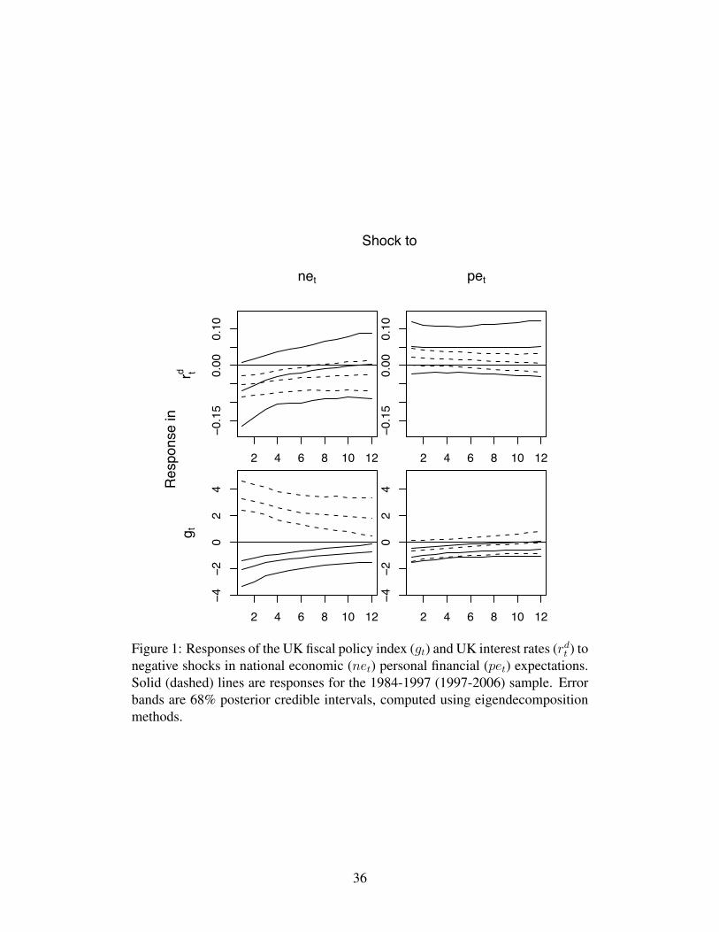
Figure 1 shows the responses of the UK interest rates (rdt ) and UK fiscal policy index (gt)
to negative shocks in economic expectations. These responses are the reactions to sudden one
standard deviation declines in national economic and personal financial expectations. Overall,
fiscal and monetary policies react to surprise changes in national economic expectations more than
to such changes in personal financial expectations in both the 1984-1997 and 1997-2006 periods.
A sudden decline in national economic expectations leads to a decrease in interest rates in both
periods, which means that the central bank attempts to stimulate the economy when economic
prospects for the whole country worsen. The reverse happens for personal expectations shocks,
which lead to higher interest rates in the Tory period, but to no significant interest rate changes in
the Labour period.
[Figure 1 about here.]
The size of the response of the central bank to shocks in economic expectations diminishes
slightly after the Bank of England was granted independence. The reaction of monetary policy to
a surprise decline in national economic expectations largely remains the same in the Tory to the
Labour period. But the response of interest rates to surprise changes in personal expectations in12The full pattern of the signs for the 12 equations of the B-SVAR model is (+ , – , + , –, +, +, +, +, +, +, +, +). The
order of equations is (et, rdt , ri
t, gt, pdt , yd
t , pit, yd
t , net, pet, at, vt). A + (–) means that shocks enter the respective
equation positively (negatively).
21
the Tory period reduces to the negligible amount of less than 0.025 percentage point change in the
Labour period.
The responses of the fiscal policy index to shocks in economic expectations yield similar re-
sults. The impact of a negative standard deviation shock in national economic expectations in the
Tory period is a decrease in government spending by an initial 2 percent decaying over 12 months.
A one standard deviation negative shock in national economic expectations in the Labour period
increases fiscal debt initially by nearly 4 percent, decaying slowly over 12 months. The implication
of this response is that fiscal policy became more responsive to shocks in national expectations after
1997, because the magnitude of the response is larger and decays more slowly in that period. The
negative response of fiscal policy to a negative shock in personal expectations is present in both
periods. The fiscal responses to personal expectations hardly differ in size across the two periods,
but are very small and significantly smaller than the responses to shocks in national expectations.
These results generate three conclusions. First, the government is responsive to sudden changes
in public opinion. Moreover, fiscal and monetary policies primarily react to citizens’ evaluations
of the country’s overall economic welfare and less to opinions about individuals’ personal well-
being. Second, there was a shift in responsiveness from monetary to fiscal policy after the Bank
of England gained independence. This is consistent with the idea that the government had to
rely on fiscal policy rather than monetary policy to satisfy citizens after the Bank of England
became independent. Third, Tory and Labour governments used fiscal policy differently. While
Tory governments decreased debt when citizens became less satisfied with the economy, Labour
governments did the opposite. This confirms the view that different ideas guided the economic
policies of the different governments. In response to sudden expressions of public dissatisfaction
with economic developments Tory governments tried to spur economic growth with orthodox fiscal
policies, while Labour governments used an expansionary fiscal strategy.
Figure 2 shows the responses of the political variables, prime minister approval (at) and vote
intentions (vt) to policy shocks in interest rates (rdt ) and fiscal policy (gt). The policy shocks enter
all equations as positive one standard deviation changes in the two samples. Surprise increases in
22
interest rates lead to no significant response in prime ministerial support in the Tory period and to
higher PM support in the Labour period, although the latter is rather small. Vote intentions respond
in a different fashion: positive shocks in interest rates increase vote intentions for the government
party in the Tory period and have a negligible impact on vote intentions in the Labour period.
Overall, this means that the effect of interest rate innovations on government support is weaker in
the latter period, presumably because citizens know that elected officials enjoy less control over
monetary policy.
[Figure 2 about here.]
The responses of vote intentions and approval to surprise fiscal policy shocks are shown in
the second column of Figure 2. Shocks to these two equations again are fiscal expansions in
both periods. So a surprise expansion in fiscal policy generates a decline in prime ministerial
support in the Tory period because the public expects a more orthodox fiscal policy from the Tory
government in times when the budget deficit is already high and perceived as a problem. In the
Labour period, an unexpected fiscal expansion increases prime ministerial support because citizens
reward fiscal expansions by the Labour government, especially in a period where the deficit is not
a serious problem. This supports the argument that the impacts of fiscal policy are inverted in the
Labour versus Tory periods because surprise contractions (expansions) in fiscal policy generate
different approval responses across the two periods. Overall, we conclude from these findings that
citizens observe policy choices by the government and take them into account when evaluating the
government’s performance. This is consistent with our results of our analysis of our models’ fits.
The response of vote intentions to fiscal shocks is similar in both periods. It declines when
there is a surprise fiscal expansion. This is not consistent with standard expectations for the Labour
period. However, it may be an expectational response. Given the UK history with inflation, citizens
may be skeptical of fiscal stimuli and therefore punish the government at election time. Note,
however that this response is never more than a whole point decline in vote intentions over 12
months.
23
Figure 3 shows the UK real economy (ydt and pd
t ) responses to positive shocks in monetary and
fiscal policy.13 Although we find that policy innovations influence output and prices, these effects
are tiny. A one standard deviation change in the policy variables does not cause a change in price
levels for monetary policy and a change of about 0.08 percent —a maximum—for fiscal policy
over 12 months. Output does not change noticeably in response to monetary policy shocks. The
results suggest that policy was largely ineffective and that the governments’ capacities to shape real
economic outcomes were limited. The magnitudes of the impacts of fiscal and monetary policy
innovations are very small. The governments’ policy innovations have virtually no impact on the
real British economy.14
[Figure 3 about here.]
Figure 4 shows the final part of the causal chain, the impacts of positive shocks to the domestic
real economy (pdt and yd
t ) on the vote intention (vt) and prime ministerial approval (at) equations.
Overall the responses of vt and at to real economic developments are fairly weak. The reaction of
prime ministerial approval to shocks in prices include zero in both periods. The reactions of these
equations to industrial production shocks are very small and do not exceed 0.1 percentage points
in either period. The effect of industrial production shocks on approval has non-zero credible
intervals during the first three to four months. We see similar results for the impact of the real
economy shocks on vote intentions. Price shocks have small effects on vote intentions during both
periods. Domestic output shocks have no sizeable effects in either period.15
13In Figure 3, the error bands cannot be distinguished from the modal impulse response because of the very small
credible region around the response.14Over 92% of the forecast variation in yd
t and pdt is due to their own innovations in both sample periods (results not
reported). Fiscal and monetary policy innovations explain at most 0.5% of the variation in these two variables in the
Tory period and at most 1.6% of the variation in both variables in the Labour period. So there is strong evidence that
the results in Figure 3 are trivial in the UK economy.15In the Tory period, the decompositions of the forecast variance (not reported) show that interest rate and fiscal
shocks generate at most 10% and 67% of the variance in at and 0.2% and 52% of the variance in vt. In the Labour
perod, the decompositions of the forecast error variance show that the interest rate and fiscal shocks generate at most
24
[Figure 4 about here.]
Conclusion
Although the connection between economic evaluations and political support for governments was
established a long time ago, the exact accountability mechanism underlying this relationship is still
unclear. Many competence models stress the importance of economic outcomes for evaluations.
Citizens infer the competence of incumbents from economic developments and rationally choose
one policymaker over another in a democratic election. Alternatively, it is possible that policies
play a more important role than often implied by theoretical models. We evaluate these hypotheses
in a Bayesian multivariate time series analysis of the British political economy since the 1980s.
Our results strongly support the idea that contemporaneous monetary and fiscal policies are
essential parts of the accountability mechanism. In comparison, observable economic outcomes
have a much smaller effect on evaluations of governments. Citizens not only take into account
observable policy adjustments when evaluating government performance, but governments also are
responsive to shifts in political evaluations. Moreover, the institutional setting determines which
information citizens use when evaluating governments. The focus on monetary policy disappears
and fiscal policy becomes primary when the central bank is granted political independence.
Our findings have implications for theoretical models of accountability and government evalu-
ations. Many competence model(s) stress the importance of outcomes for these evaluation mech-
anisms, but ignore or assign little relevance to policies. This is inconsistent with our findings.
One implication is that the role of observable and unobservable policies and their exact impact
on the economy should be specified more clearly. In particular, how incumbents can vary in their
unobservable “decisions” (Duch and Stevenson, 2008) and how these decisions affect economic
performance is unclear. We need a better understanding of what the options of incumbents are,
which of their decisions are observable and which ones are not. The role of fiscal and other poli-
0.2% and 81% of the variance in at and less than 0.1% and 62% of the variance in vt. These results are consistent
with the shift from monetary to fiscal policy tools after 1997.
25
cies should be specified in this context. As it is formulated now, the nature of economic policies
bearing on democratic accountability remains obscure.16
With respect to future empirical research, additional cases should be studied. The first step is to
analyze democratic accountability in countries where there still is some a moderate level of clarity
of responsibility and policy transparency like the U.S. Recent research suggests that, unlike their
British counterparts, a majority of Americans believe in their government’s capability to manage
economic developments (Hellwig, Ringsmuth and Freeman, 2008). Building and analyzing a B-
SVAR model for the American political economy would provide a test of these beliefs. Our time
series model also should be integrated more fully with a political, dynamic stochastic general equi-
librium model of the UK (Houser and Freeman, 2001). This could allow for deeper historical and
policy counterfactual analyses. In this context, it is important that, when (if) they become avail-
able, we analyze real time macroeconomic time series for the U.K. and U.S. We do not include
an analysis of such time series here because it possible that many citizens use some kind of ’bias
adjustment’ in assessing reports of policy choice and policy outcomes (Garratt and Vahey, 2006)
and real time macroeconomic data for several of our key variables are available only in more tem-
porally aggregated (quarterly) form. Also real time data sets do not include all the series we need
to replicate our analysis. For instance, real time British data are not available for fiscal measure
before 1990 (cf. Egginton, Pick and Vahey, 2002). Nonetheless, revision of macroeconomic time
series is an important methodological issue. It should be addressed by political economists in the
future.
16The finding that fiscal policy plays a major role for the evaluation of government competence is consistent with
the early model by Rogoff (1990).
26
Appendix: Estimation Details of the B-SVAR Model
The Bayesian structural vector autoregresison (B-SVAR) models outlined earlier and this appendix
were estimated using the methods discussed in Brandt and Freeman (2006, 2009). The models are
estimated with the following steps:
1. Specify the restrictions in the A0 matrix. These allow us to determine which contemporane-
ous effects enter which equations (see the next section for more details).
2. Specify the hyperparameters for the prior distribution of the models’ parameters. The mean
for the prior distribution of the parameters is centered on a random walk model where the
prior mean for A1 is an identity matrix and the prior mean on the lag coefficients for lags
2 through p are zero. The prior variance of these parameters are based on the values of the
standard deviations discussed in footnote 8. The prior variance for the coefficient for the �th
lag of variable j in equation i is
�λ0λ1
σj�λ3
�2
where λ0 is a discount factor for the sample variance, λ1 is the standard around the first lag
coefficients, �λ3 is a factor that shinks the prior variance for higher order lags toward zero and
σj is the sample standard deviation of variable j. In the analysis presented multiple priors
were analyzed and the main conclusions vary sensibly for larger and smaller prior variances.
3. Use numerical optimization to find the peak of the posterior distribution of the models’ pa-
rameters. Because this is a non-recursive SVAR model, the maximum likelihood or Bayesian
posterior solution cannot be found using the standard equation-by-equation estimator used
for reduced form VARs.
4. Sample from the posterior mode identified in the previous step using the Gibbs sampler
algorithm for B-SVAR models proposed by Waggoner and Zha (2003a). After an appropriate
27
burnin period, a sample of 25000 draws is taken from the posterior distribution of each
model.
5. Compute the marginal data density using the posterior sample. These allow us to construct
the Bayes factors and the elements in Table 1.
6. Based on the posterior sample of coefficients, compute and plot the moving average re-
sponses and their error bands using the methods in Brandt and Freeman (2006). The moving
average responses allow us to track out the impact of standardized shocks to see the dynamic
responses of any equation to a shock to a given variable. These are presented graphically
since they provide concise way of capturing the information in the estimated m equations
with p lags. In total, there are m2p + 2m = 1226 + 24 = 888 regression parameters plus
those estimated in A0.
A significant effort went into the sensitivity analysis of these models. Other values for the prior
hyperparameters were evaluated. The sensitivity analyses also tried different lag length specifica-
tions (6 versus 12 lags), models without the national and personal economic expectations measures,
models without the open economy equations for the US time series, and models with a measure
of UK debt rather than the net cash position variable reported here. The results from these other
specifications are consistent with those reported here.
Appendix: Specification of the SVAR models
Deriving the different, theoretically motivated structural relationships for the endogenous variables
in the polity and the economy in A0, relies on existing research in political science and the new
open macroeconomics. The submatrices of Equation 2 define the political and economic relations
in AP0 and AE
0 .
For the polity we expect that contemporaneous national economic expectations affect personal
economic expectation, but not vice versa. This is because aggregate welfare should affect indi-
28
vidual well-being, but individual financial wealth does not matter for the whole country. The two
economic expectations variables together affect approval to the chief executive and vote intentions
for the government (Sanders, 1991; MacKuen, Erikson and Stimson, 1992; Clarke and Stewart,
1995). We treat executive approval as weakly exogenous to vote intentions. This is consistent
with results from previous research (Clarke and Stewart, 1995; Clarke, Ho and Stewart, 2000);
it is theoretically plausible because citizens are more likely to vote for a government if they are
satisfied with its executive. In contrast, the performance of the chief executive should not depend
contemporaneously on the percentage of citizens who want to vote for the government.
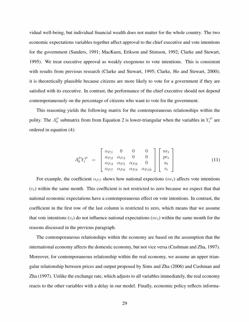
This reasoning yields the following matrix for the contemporaneous relationships within the
polity. The AP0 submatrix from from Equation 2 is lower-triangular when the variables in Y P
t are
ordered in equation (4):
AP0 Y P
t =
αP,1 0 0 0αP,2 αP,3 0 0αP,4 αP,5 αP,6 0αP,7 αP,8 αP,9 αP,10
net
pet
at
vt
(11)
For example, the coefficient αP,7 shows how national expections (net) affects vote intentions
(vt) within the same month. This coefficient is not restricted to zero because we expect that that
national economic expectations have a contemporaneous effect on vote intentions. In contrast, the
coefficient in the first row of the last column is restricted to zero, which means that we assume
that vote intentions (vt) do not influence national expectations (net) within the same month for the
reasons discussed in the previous paragraph.
The contemporaneous relationships within the economy are based on the assumption that the
international economy affects the domestic economy, but not vice versa (Cushman and Zha, 1997).
Moreover, for contemporaneous relationship within the real economy, we assume an upper trian-
gular relationship between prices and output proposed by Sims and Zha (2006) and Cushman and
Zha (1997). Unlike the exchange rate, which adjusts to all variables immediately, the real economy
reacts to the other variables with a delay in our model. Finally, economic policy reflects informa-
29
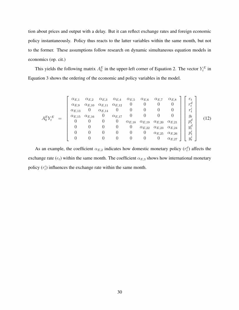
tion about prices and output with a delay. But it can reflect exchange rates and foreign economic
policy instantaneously. Policy thus reacts to the latter variables within the same month, but not
to the former. These assumptions follow research on dynamic simultaneous equation models in
economics (op. cit.)
This yields the following matrix AE0 in the upper-left corner of Equation 2. The vector Y E
t in
Equation 3 shows the ordering of the economic and policy variables in the model.
AE0 Y E
t =
αE,1 αE,2 αE,3 αE,4 αE,5 αE,6 αE,7 αE,8
αE,9 αE,10 αE,11 αE,12 0 0 0 0αE,13 0 αE,14 0 0 0 0 0αE,15 αE,16 0 αE,17 0 0 0 0
0 0 0 0 αE,18 αE,19 αE,20 αE,21
0 0 0 0 0 αE,22 αE,23 αE,24
0 0 0 0 0 0 αE,25 αE,26
0 0 0 0 0 0 0 αE,27
et
rdt
rit
gt
pdt
ydt
pit
yit
(12)
As an example, the coefficient αE,2 indicates how domestic monetary policy (rdt ) affects the
exchange rate (et) within the same month. The coefficient αE,3 shows how international monetary
policy (rit) influences the exchange rate within the same month.
30
References
Alesina, Alberto and Howard Rosenthal. 1995. Partisan Politics, Divided Government, and the
Economy. Cambridge University Press.
Alt, James E. and David Dreyer Lassen. 2006. “Transparency, Political Polarization, and Political
Budget Cycles in OECD Countries.” American Journal of Political Science 50(3):530–550.
Bernhard, William and David Leblang. 2006. “Polls and Pounds: Exchange Rate Volatility and
Domestic Political Competition in Britain.” Quarterly Journal of Political Science 1(1):25–47.
Bernhard, William, Lawrence J. Broz and William R. Clark. 2002. “The Political Economy of
Monetary Institutions.” International Organization 56(4):693–724.
Brandt, Patrick T. and John R. Freeman. 2006. “Advances in Bayesian Time Series Modeling
and the Study of Politics: Theory Testing, Forecasting, and Policy Analysis.” Political Analysis
14(1):1–36.
Brandt, Patrick T. and John R. Freeman. 2009. “Modeling Macro Political Dynamics.” Political
Analysis 17(2):113–142.
Brandt, Patrick T. and John T. Williams. 2007. Multiple Time Series Models. Sage.
Clark, William R. and Mark Hallerberg. 2000. “Mobile Capital, Domestic Institutions, and Elec-
torally Induced Monetary and Fiscal Policy.” American Political Science Review 94(2):323–346.
Clarke, Harold D., David Sanders, Marianne C. Stewart and Paul F. Whiteley. 2004. Political
Choice in Britain. Oxford University Press.
Clarke, Harold, Karl Ho and Marianne C. Stewart. 2000. “Major’s lesser (not Minor) Effects:
Prime Ministerial Approval and Governing Party Support in Britain Since 1979.” Electoral Stud-
ies 19:255–273.
31

Clarke, Harold and Marianne C. Stewart. 1995. “Economic Evaluations, Prime Ministerial Ap-
proval and Governing Party Support: Rival Models Reconsidered.” British Journal of Political
Science 25(2):145–170.
Cushman, David O. and Tao Zha. 1997. “Identifying Monetary Policy in a Small Open Economy
under Flexible Exchange Rates.” Journal of Monetary Economics 39(3):433–448.
Duch, Raymond M. and Randolph T. Stevenson. 2008. The Economic Vote: How Political and
Economic Institutions Condition Election Results. Cambridge University Press.
Egginton, Don M., Andreas Pick and Shaun P. Vahey. 2002. “Keep it Real!: A Real-Time UK
Macro Data Set.” Economics Letters 77:15–20.
Erikson, Robert S., Michael B. MacKuen and James A. Stimson. 2002. The Macro Polity. Cam-
bridge University Press.
Freeman, John R., John T. Williams and Tse min Lin. 1989. “Vector Autoregression and the Study
of Politics.” American Journal of Political Science 33(4):842–877.
Garratt, Anthony and Shaun P. Vahey. 2006. “UK Real-Time Macro Data Characteristics.” The
Economic Journal 116:F119–F135.
Hallerberg, Mark and Jurgen Von Hagen. 1999. Electoral Institutions, Cabinet Negotiations and
Budget Deficits within the European Union. In Fiscal Institutions and Fiscal Performance, ed.
Jurgen Von Hagen. University of Chicago Press pp. 209–232.
Hellwig, Timothy, Eve Ringsmuth and John R. Freeman. 2008. “The American Public and the
Room to Maneuver: Responsibility Attributions and Policy Efficacy in an Era of Globalization.”
International Studies Quarterly 52:855–880.
Houser, Daniel and John R. Freeman. 2001. “Economic Consequences of Political Approval Man-
agement in Comparative Perspective.” Journal of Comparative Economics 29(4):692–721.
32
Iversen, Torben. 1998a. “Wage Bargaining, Central Bank Independence, and the Real Effect of
Money.” International Organization 52(3):469–504.
Iversen, Torben. 1998b. “Wage Bargaining, Hard Money and Economic Performance: Theory and
Evidence for Organized Market Economies.” British Journal of Political Science 28(1):31–61.
Kass, Robert E. and Adrian E. Raftery. 1995. “Bayes Factors.” Journal of the American Statistical
Assocation 90(430):773–795.
Kim, Soyoung. 2001. “International Transmission of U.S. Monetary Policy Shocks: Evidence
from VAR’s.” Journal of Monetary Economics 48(2):339–372.
Leeper, Eric M., Christopher A. Sims and Tao A. Zha. 1996. “What Does Monetary Policy Do?”
Brookings Papers on Economic Activity 1996(2):1–63.
MacKuen, Michael B., Robert S. Erikson and James A. Stimson. 1992. “Peasants or Bankers? The
American Electorate and the US Economy.” American Political Science Review 86(3):597–611.
Obstfeld, Maurice and Kenneth Rogoff. 1995. “Exchange Rate Dynamics Redux.” Journal of
Political Economy 103(3):624–660.
O’Mahony, Angela. 2008. “Engeneering Good Times: Fiscal Manipulation in a Global Economy.”
Manuscript, University of British Columbia.
Persson, Torsten and Guido Tabellini. 1990. Macroeconomic Policy, Credibility, and Politics.
Harwood Academic.
Powell, G. Bingham and Guy D. Whitten. 1993. “A Cross-National Analysis of Economic Voting:
Taking Account of the Political Context.” American Journal of Political Science 37(2):391–414.
Rogoff, Kenneth. 1990. “Equilibrium Political Budget Cycles.” American Economic Review
80(1):21–36.
33
Sanders, David. 1991. “Government Popularity and the Next General Election.” Political Quarterly
62(2):235–261.
Sanders, David. 2005. “The Political Economy of UK Party Support, 1997-2004: Forecasts for the
2005 General Election.” Journal of Elections, Public Opinion, and Parties 15(1):47–71.
Sattler, Thomas, John R. Freeman and Patrick T. Brandt. 2008. “Political Accountability and the
Room to Maneuver: A Search for a Causal Chain.” Comparative Political Studies 41(9):1212–
1238.
Sims, Christopher A. 1972. “Money, Income, and Causality.” American Economic Review
62(4):540–552.
Sims, Christopher A. 1980. “Macroeconomics and Reality.” Econometrica 48(1):1–48.
Sims, Christopher A., Daniel F. Waggoner and Tao A. Zha. 2008. “Methods for Inference in Large
Multiple-Equation Markov-Switching Models.” Journal of Econometrics 146(2):255–274.
Sims, Christopher A., James H. Stock and Mark W. Watson. 1990. “Inference in Linear Time
Series Models with Some Unit Roots.” Econometrica 58(1):113–144.
Sims, Christopher A. and Tao A. Zha. 1998. “Bayesian Methods for Dynamic Multivariate Mod-
els.” International Economic Review 39:949–968.
Sims, Christopher A. and Tao A. Zha. 1999. “Error Bands for Impulse Responses.” Econometrica
67(5):1113–1156.
Sims, Christopher A. and Tao A. Zha. 2006. “Does Monetary Policy Generate Recessions?”
Macroeconomic Dynamics 10(2):231–272.
Soroka, Stuart N. and Christopher Wlezien. 2005. “Opinion-Policy Dynamics: Public Preferences
and Public Expenditures in the United Kingdom.” British Journal of Political Science 35(4):665–
689.
34
Stimson, James A., Michael B. MacKuen and Robert S. Erikson. 1995. “Dynamic Representation.”
American Political Science Review 89(3):543–565.
Waggoner, Daniel F. and Tao A. Zha. 2003a. “A Gibbs Sampler for Structural Vector Autoregres-
sions.” Journal of Dynamics and Control 28(2):349–366.
Waggoner, Daniel F. and Tao A. Zha. 2003b. “Likelihood Preserving Normalization in Multiple
Equation Models.” Journal of Econometrics 114(2):329–347.
Williams, John T. 1990. “The Political Manipulation of Macroeconomic Policy.” American Politi-
cal Science Review 84:757–795.
Wlezien, Christopher. 2004. “Patterns of Representation: Dynamics of Public Preferences and
Policy.” Journal of Politics 66(1):1–24.
35
2 4 6 8 10 12
−0.1
50.
000.
10
r td
net
2 4 6 8 10 12
−4−2
02
4
g t
2 4 6 8 10 12
−0.1
50.
000.
10
pet
2 4 6 8 10 12
−4−2
02
4Res
pons
e in
Shock to
Figure 1: Responses of the UK fiscal policy index (gt) and UK interest rates (rdt ) to
negative shocks in national economic (net) personal financial (pet) expectations.Solid (dashed) lines are responses for the 1984-1997 (1997-2006) sample. Errorbands are 68% posterior credible intervals, computed using eigendecompositionmethods.
36
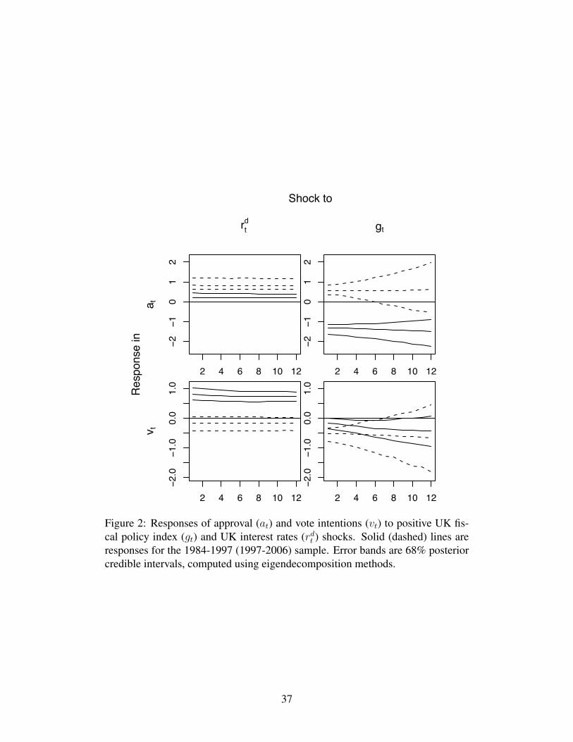
2 4 6 8 10 12
−2−1
01
2
a t
rtd
2 4 6 8 10 12
−2.0
−1.0
0.0
1.0
v t
2 4 6 8 10 12
−2−1
01
2
gt
2 4 6 8 10 12
−2.0
−1.0
0.0
1.0
Res
pons
e in
Shock to
Figure 2: Responses of approval (at) and vote intentions (vt) to positive UK fis-cal policy index (gt) and UK interest rates (rd
t ) shocks. Solid (dashed) lines areresponses for the 1984-1997 (1997-2006) sample. Error bands are 68% posteriorcredible intervals, computed using eigendecomposition methods.
37
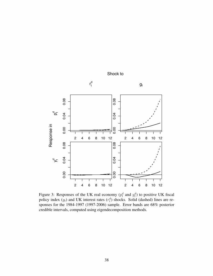
2 4 6 8 10 12
0.00
0.04
0.08
p td
rtd
2 4 6 8 10 12
0.00
0.04
0.08
y td
2 4 6 8 10 12
0.00
0.04
0.08
gt
2 4 6 8 10 12
0.00
0.04
0.08Res
pons
e in
Shock to
Figure 3: Responses of the UK real economy (pdt and yd
t ) to positive UK fiscalpolicy index (gt) and UK interest rates (rd
t ) shocks. Solid (dashed) lines are re-sponses for the 1984-1997 (1997-2006) sample. Error bands are 68% posteriorcredible intervals, computed using eigendecomposition methods.
38
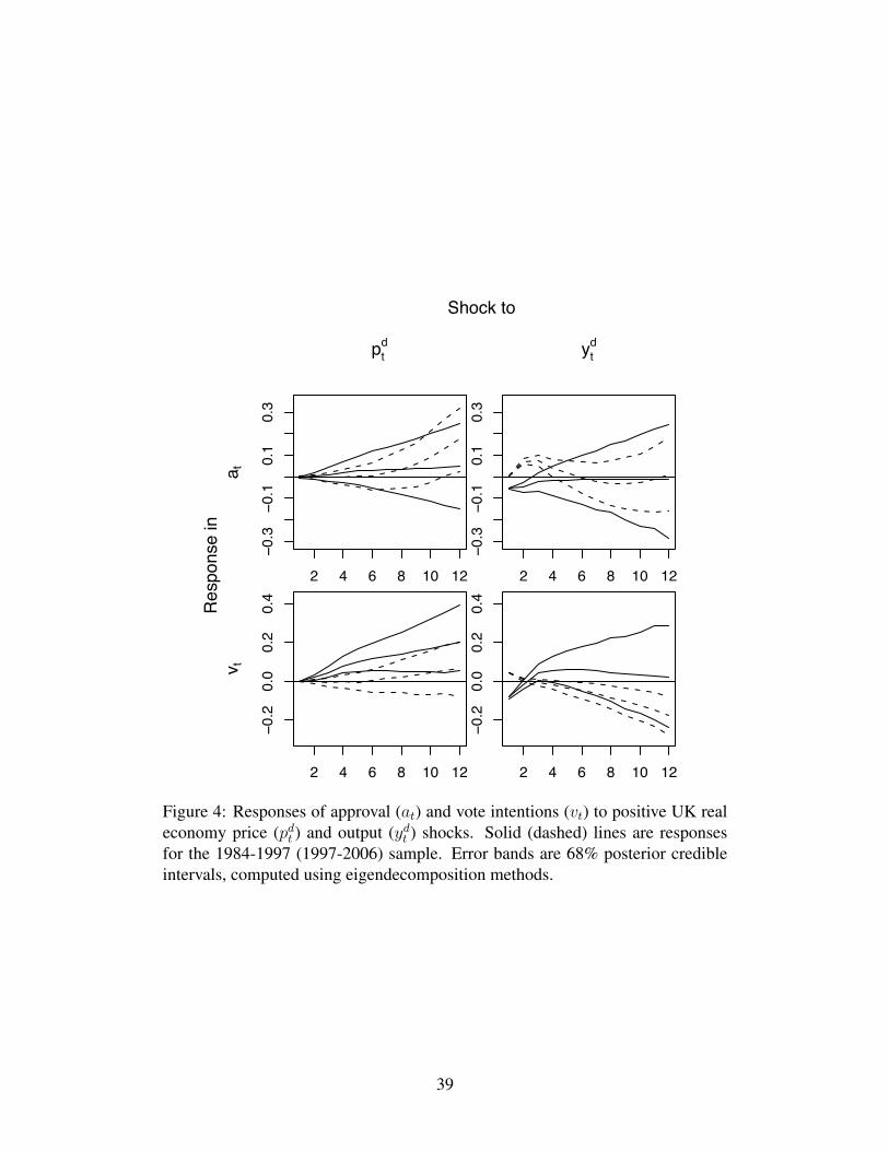
2 4 6 8 10 12
−0.3
−0.1
0.1
0.3
a t
ptd
2 4 6 8 10 12
−0.2
0.0
0.2
0.4
v t
2 4 6 8 10 12
−0.3
−0.1
0.1
0.3
ytd
2 4 6 8 10 12
−0.2
0.0
0.2
0.4Res
pons
e in
Shock to
Figure 4: Responses of approval (at) and vote intentions (vt) to positive UK realeconomy price (pd
t ) and output (ydt ) shocks. Solid (dashed) lines are responses
for the 1984-1997 (1997-2006) sample. Error bands are 68% posterior credibleintervals, computed using eigendecomposition methods.
39
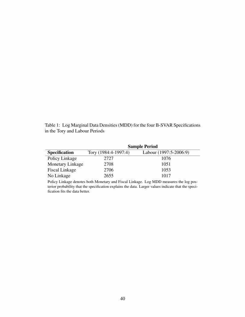
Table 1: Log Marginal Data Densities (MDD) for the four B-SVAR Specificationsin the Tory and Labour Periods
Sample Period
Specification Tory (1984:4-1997:4) Labour (1997:5-2006:9)Policy Linkage 2727 1076Monetary Linkage 2708 1051Fiscal Linkage 2706 1053No Linkage 2655 1017Policy Linkage denotes both Monetary and Fiscal Linkage. Log MDD measures the log pos-terior probability that the specification explains the data. Larger values indicate that the speci-fication fits the data better.
40